A Concise History of World Population

Welcome message from author
This document is posted to help you gain knowledge. Please leave a comment to let me know what you think about it! Share it to your friends and learn new things together.
Transcript

A Concise History of World Population
A Concise History of World Population
Sixth Edition
Massimo Livi‐Bacci
This sixth edition first published 2017© 2017 John Wiley & Sons Ltd
Edition history: 5e: John Wiley & Sons Ltd, 2012; 4e: Blackwell Publishing Ltd, 2007; 3e, 2e, 1e: Blackwell Publishers Ltd, 2001, 1997, 1992
Registered OfficeJohn Wiley & Sons Ltd, The Atrium, Southern Gate, Chichester, West Sussex, PO19 8SQ, UK
Editorial Offices350 Main Street, Malden, MA 02148‐5020, USA9600 Garsington Road, Oxford, OX4 2DQ, UKThe Atrium, Southern Gate, Chichester, West Sussex, PO19 8SQ, UK
For details of our global editorial offices, for customer services, and for information about how to apply for permission to reuse the copyright material in this book please see our website at www.wiley.com/wiley‐blackwell.
The right of Massimo Livi‐Bacci to be identified as the author of this work has been asserted in accordance with the UK Copyright, Designs and Patents Act 1988.
All rights reserved. No part of this publication may be reproduced, stored in a retrieval system, or transmitted, in any form or by any means, electronic, mechanical, photocopying, recording or otherwise, except as permitted by the UK Copyright, Designs and Patents Act 1988, without the prior permission of the publisher.
Wiley also publishes its books in a variety of electronic formats. Some content that appears in print may not be available in electronic books.
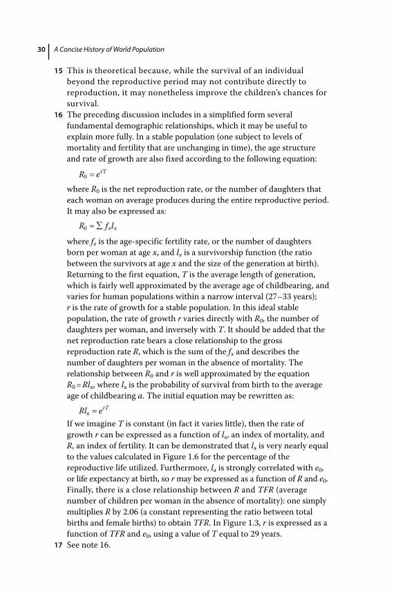
Designations used by companies to distinguish their products are often claimed as trademarks. All brand names and product names used in this book are trade names, service marks, trademarks or registered trademarks of their respective owners. The publisher is not associated with any product or vendor mentioned in this book.
Limit of Liability/Disclaimer of Warranty: While the publisher and author have used their best efforts in preparing this book, they make no representations or warranties with respect to the accuracy or completeness of the contents of this book and specifically disclaim any implied warranties of merchantability or fitness for a particular purpose. It is sold on the understanding that the publisher is not engaged in rendering professional services and neither the publisher nor the author shall be liable for damages arising herefrom. If professional advice or other expert assistance is required, the services of a competent professional should be sought.
Library of Congress Cataloging‐in‐Publication Data
Names: Livi-Bacci, Massimo, author.Title: A concise history of world population / Massimo Livi-Bacci.Other titles: Storia minima della popolazione del mondo. EnglishDescription: Sixth edition. | Hoboken, NJ : John Wiley & Sons, Inc., 2017. |
Includes bibliographical references and index.Identifiers: LCCN 2016034598 (print) | LCCN 2016047998 (ebook) |
ISBN 9781119029274 (pbk.) | ISBN 9781119029298 (pdf) | ISBN 9781119029304 (epub)
Subjects: LCSH: Population–History.Classification: LCC HB871 .L56513 2017 (print) | LCC HB871 (ebook) | DDC 304.6–dc23LC record available at https://lccn.loc.gov/2016034598
A catalogue record for this book is available from the British Library.
Cover image: Rawpixel/gettyimagesCover design by Wiley
Set in size 10/12pt Warnock by SPi Global, Pondicherry, India
10 9 8 7 6 5 4 3 2 1
v
Contents
Preface ixAcknowledgment xi
1 The Space and Strategy of Demographic Growth 11.1 Humans and Animals 11.2 Divide and Multiply 51.3 Jacopo Bichi and Domenica Del Buono, Jean Guyon,
and Mathurine Robin 71.4 Reproduction and Survival 91.5 The Space of Growth 171.6 Environmental Constraints 191.7 A Few Figures 24 Notes 27 Further Reading 32
2 Demographic Growth: Between Choice and Constraint 332.1 Constraint, Choice, Adaptation 332.2 From Hunters to Farmers: The Neolithic Demographic
Transition 352.3 Black Death and Demographic Decline in Europe 422.4 The Tragedy of the American Indios: Old Microbes
and New Populations 472.5 Africa, America, and the Slave Trade 532.6 The French Canadians: A Demographic Success Story 572.7 Ireland and Japan: Two Islands, Two Histories 612.8 On the Threshold of the Contemporary World:
China and Europe 67 Notes 73 Further Reading 84
Contentsvi
3 Land, Labor, and Population 853.1 Diminishing Returns and Demographic Growth 853.2 Historical Confirmations 893.3 Demographic Pressure and Economic Development 943.4 More on Demographic Pressure and Development:
Examples from the Stone Age to the Present Day 983.5 Space, Land, and Development 1013.6 Population Size and Prosperity 1083.7 Increasing or Decreasing Returns? 112 Notes 113 Further Reading 117
4 Toward Order and Efficiency: The Recent Demography of Europe and the Developed World 119
4.1 From Waste to Economy 1194.2 From Disorder to Order: The Lengthening of Life 1244.3 From High to Low Fertility 1314.4 European Emigration: A Unique Phenomenon 1374.5 A Summing Up: The Results of the Transition 1434.6 Theoretical Considerations on the Relationship between
Demographic and Economic Growth 1464.7 More on the Relationship between Demographic
and Economic Growth: Empirical Observations 150 Notes 157 Further Reading 164
5 The Populations of Poor Countries 1675.1 An Extraordinary Phase 1675.2 The Conditions of Survival 1725.3 A Brief Geography of Fertility 1795.4 The Conditions and Prospects for Fertility Decline
and Demographic Policy 1845.5 India and China 1915.6 Fertilia and Sterilia 2015.7 Explaining a Paradox 205 Notes 212 Further Reading 222
6 The Future 2256.1 Population and Self‐Regulation 2256.2 The Numbers of the Future 2276.3 The North–South Divide and International Migration 2336.4 On Sustainability of Extended Survival 2426.5 The Moving Limits 251

Contents vii
6.6 Non‐Renewable Resources and the Parable of Pauperia and Tycoonia 255
6.7 Food for All? 2596.8 Space and Environment in a Smaller Planet 2656.9 Calculations and Values 270 Notes 274
Major Scientific Journals for Further Reading 281Index 283
ix
Preface
Why is the present population of the world 7 billion1 and not several orders of magnitude greater or smaller? For thousands of years prior to the invention of agriculture the human species must have numbered a thousandth of what it does today; and there are those who maintain that our planet, given the available resources, could comfortably accommo-date a population 10 times larger than it does at present. What are the factors that through the ages determined demographic growth? How is the difficult balance with resources and environment maintained? These are fairly old questions, confronted for the first time in a modern form by Malthus, who, not by accident, inspired the work of Darwin.
In the pages of this “concise history” I intend to address these fundamental questions, discussing the underlying suppositions, the proposed solutions, the points already clarified, and those still requiring investigation. The reader will find here a general discussion of demographic development and, I hope, a guide to understanding the mechanisms that, through the ages, have determined population growth, stagnation, or decline.
Since the invention of fire the human species has sought to modify the environment and enrich the resources it provides. In the very long term (millennia), humanity has grown numerically in relative harmony with available resources. Certainly the system of hunting and gathering could not have allowed the survival of many more than several million people, just as the European system of agriculture could only, with great difficulty, have supported more than the 100 million inhabitants who lived on the continent prior to the Industrial Revolution. However, in shorter spans of time (centuries or generations) this equilibrium is not so obvious, for two fundamental reasons. The first is the recurrent action of catastrophic events – epidemics, climatic, or natural disasters – which alter radically one term of the population–resources equation. The second lies in the fact that the demographic mechanisms that determine reproductive intensity, and so demographic growth, change slowly and do not “adapt” easily to rapidly evolving environmental conditions. It is frequently claimed that
Prefacex
the human species is equipped with “self‐regulating” mechanisms that allow for the speedy reestablishment of the balance between numbers and resources. However, this is only partially true, as these mechanisms – when they do work – are imperfect (and of varying efficiency from population to population and from one age to another), so much so that entire popu-lations have disappeared – a clear sign of the failure of all attempts at regulation.
In the following pages I devote a great deal of attention to the function-ing, in various contexts and periods, of the mechanisms that determine the always precarious balance between population and resources. In order to do this I have addressed problems and topics – from biology to economics – rarely touched upon in demographic works, and so have risked losing the depth of this study for the breadth of its extension. A worthwhile risk, given the complexity of population change’s forces.
Note
1 Throughout the text I use US billion to equal 1,000,000,000.

xi
Acknowledgment
This publication was made possible through the cooperation of Biblioteca Italia, a Giovanni Agnelli Foundation program for the diffusion of Italian culture.
1
A Concise History of World Population, Sixth Edition. Massimo Livi-Bacci. © 2017 John Wiley & Sons Ltd. Published 2017 by John Wiley & Sons Ltd.
The Space and Strategy of Demographic Growth
1.1 Humans and Animals
Throughout human history population has been synonymous with prosperity, stability, and security. A valley or plain teeming with houses, farms, and villages has always been a sign of well‐being. Traveling from Verona to Vicenza, Goethe remarked with pleasure: “One sees a continuous range of foothills … dotted with villages, castles and isolated houses … we drove on a wide, straight and well‐kept road through fertile fields … The road is much used and by every sort of person.”1 The effects of a long history of good government were evident, much as in the ordered Sienese fourteenth‐century landscapes of the Lorenzetti brothers. Similarly, Cortés was unable to restrain his enthusiasm when he gazed over the valley of Mexico and saw the lagoons bordered by villages and trafficked by canoes, the great city, and the market (in a square more than double the size of the entire city of Salamanca) that “accommodated every day more than sixty thousand individuals who bought and sold every imaginable sort of merchandise.”2
This should come as no surprise. A densely populated region is implicit proof of a stable social order, of nonprecarious human relations, and of well‐utilized natural resources. Only a large population can mobilize the human resources necessary to build houses, cities, roads, bridges, ports, and canals. If anything, it is abandonment and desertion rather than abundant population that has historically dismayed the traveler.
Population, then, might be seen as a crude index of prosperity. The million inhabitants of the Paleolithic Age, the 10 million of the Neolithic Age, the 100 million of the Bronze Age, the billion of the Industrial Revolution, or the 10 billion that we may attain by mid twenty‐first century certainly represent more than simple demographic growth. Even these few figures tell us that demographic growth has not been uniform over time. Periods of expansion have alternated with others of stagnation
1
A Concise History of World Population 2
and even decline; and the interpretation of these, even for relatively recent historical periods, is not an easy task. We must answer questions that are as straightforward in appearance as they are complex in substance: Why are we 7 billion today and not more or less, say 100 billion or 100 million? Why has demographic growth, from prehistoric times to the present, followed a particular path rather than any of numerous other possibilities? These questions are difficult but worth considering, since the numerical progress of population has been, if not dictated, at least constrained by many forces and obstacles that have determined the general direction of that path. To begin with, we can categorize these forces and obstacles as biological and environmental. The former are linked to the laws of mortality and reproduction that determine the rate of demographic growth; the latter determines the resistance that these laws encounter and further regulates the rate of growth. Moreover, biological and environmental factors affect one another reciprocally and so are not independent of one another.
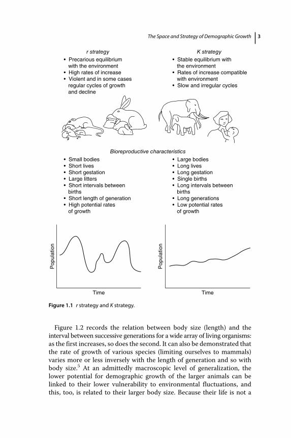
Every living collectivity develops particular strategies of survival and reproduction, which translate into potential and effective growth rates of varying velocity. A brief analysis of these strategies will serve as the best introduction to consideration of the specific case of the human species. Biologists have identified two large categories of vital strategies, called r and K, which actually represent simplifications of a continuum.3 Insects, fish, and some small mammals practice an r‐strategy: these organisms live in generally unstable environments and take advantage of favorable periods (annually or seasonally) to reproduce prolifically, even though the probability of offspring survival is small. It is just because of this environmental instability, however, that they must depend upon large numbers, because “life is a lottery and it makes sense simply to buy many tickets.”4 r‐strategy organisms go through many violent cycles with phases of rapid increase and decrease.
A much different strategy is that practiced by K‐type organisms – mammals, particularly medium and large ones, and some birds – who colonize relatively stable environments, albeit populated with competitors, predators, and parasites. K‐strategy organisms are forced by selective and environmental pressure to compete for survival, which in turn requires considerable investment of time and energy for the raising of offspring. This investment is only possible if the number of offspring is small.
r and K strategies characterize two well‐differentiated groups of organisms (Figure 1.1). The first are suited to small animals having a short life span, minimal intervals between generations, brief gestation periods, short intervals between births, and large litters. K strategies, on the other hand, are associated with larger animals, long life spans, long intervals between generations and between births, and single births.
The Space and Strategy of Demographic Growth 3
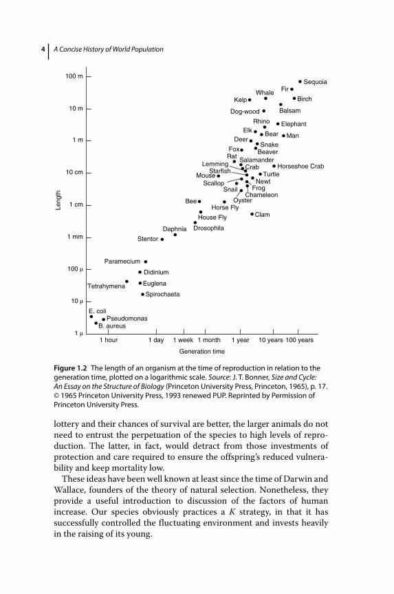
Figure 1.2 records the relation between body size (length) and the interval between successive generations for a wide array of living organisms: as the first increases, so does the second. It can also be demonstrated that the rate of growth of various species (limiting ourselves to mammals) varies more or less inversely with the length of generation and so with body size.5 At an admittedly macroscopic level of generalization, the lower potential for demographic growth of the larger animals can be linked to their lower vulnerability to environmental fluctuations, and this, too, is related to their larger body size. Because their life is not a
r strategy K strategy• Precarious equilibrium with the environment• High rates of increase• Violent and in some cases regular cycles of growth and decline
• Stable equilibrium with the environment• Rates of increase compatible with environment• Slow and irregular cycles
• Small bodies• Short lives• Short gestation• Large litters• Short intervals between births• Short length of generation• High potential rates of growth
• Large bodies• Long lives• Long gestation• Single births• Long intervals between births• Long generations• Low potential rates of growth
TimeTime
Pop
ulat
ion
Pop
ulat
ion
Bioreproductive characteristics
Figure 1.1 r strategy and K strategy.
A Concise History of World Population 4
lottery and their chances of survival are better, the larger animals do not need to entrust the perpetuation of the species to high levels of reproduction. The latter, in fact, would detract from those investments of protection and care required to ensure the offspring’s reduced vulnerability and keep mortality low.
These ideas have been well known at least since the time of Darwin and Wallace, founders of the theory of natural selection. Nonetheless, they provide a useful introduction to discussion of the factors of human increase. Our species obviously practices a K strategy, in that it has successfully controlled the fluctuating environment and invests heavily in the raising of its young.
100 m
10 m
1 m
10 cm
1 cm
1 mm
100 µ
10 µ
1 µ1 hour 1 day 1 week 1 month 1 year 10 years 100 years
Generation time
Leng
th
SequoiaFirWhale
Kelp Birch
BalsamDog-wood
Rhino ElephantElk
DeerBear Man
SnakeFox Beaver
RatLemming
Salamander
StarfishHorseshoe CrabCrab
TurtleScallop Newt
Snail
Mouse
FrogChameleon
OysterBeeHorse Fly
Clam
DrosophilaDaphnia
Stentor
Paramecium
Didinium
Tetrahymena Euglena
Spirochaeta
E. coliPseudomonas
B. aureus
House Fly
Figure 1.2 The length of an organism at the time of reproduction in relation to the generation time, plotted on a logarithmic scale. Source: J. T. Bonner, Size and Cycle: An Essay on the Structure of Biology (Princeton University Press, Princeton, 1965), p. 17. © 1965 Princeton University Press, 1993 renewed PUP. Reprinted by Permission of Princeton University Press.
The Space and Strategy of Demographic Growth 5
Two principles will be particularly helpful for the purpose of confronting the arguments of the following pages. The first concerns the relation between population and environment; this should be understood broadly to include all the factors – physical environment, climate, availability of food, and so on – that determine survival. The second concerns the relation between reproduction and mortality insofar as the latter is a function of parental investment, which in turn relates inversely to reproductive intensity.
1.2 Divide and Multiply
Many animal species are subject to rapid and violent cycles that increase or decrease their numbers by factors of 100, 1,000, 10,000, or even more in a brief period. The 4‐year cycle of the Scandinavian lemming is well known, as are those of the Canadian predators (10 years) and many infesting insects of temperate woods and forests (4–12 years). In Australia, “in certain years the introduced domestic mouse multiplies enormously. The mice swarm in crops and haystacks, and literal bucketfuls can be caught in a single night. Hawks, owls and cats flourish at their expense … but all these enemies have little effect in reducing the numbers. As a rule the plague ends rather suddenly. A few dead mice are found on the ground and the numbers dwindle rapidly to, or below, normal.”6 Other species maintain equilibrium. Gilbert White observed two centuries ago that eight pairs of swallows flew round the belfry of the church in the village of Selborne, just as is the case today.7 There are, then, both populations in rapid growth or decline and populations that are more or less stable.
The human species varies relatively slowly in time. Nonetheless, as we shall see below, long cycles of growth do alternate with others of decline, and the latter have even led to extinction for certain groups. For example, the population of Mesoamerica was reduced to a fraction of its original size during the century that followed the Spanish conquest (initiated at the beginning of the sixteenth century), while that of the conquering Spaniards grew by half. Other populations have disappeared entirely or almost entirely – the population of Santo Domingo after the landing of Columbus, or that of Tasmania following contact with the first explorers and settlers – while at the same time others nearby have continued to increase and prosper. In more recent times, the population of England and Wales multiplied sixfold between 1750 and 1900, while that of France in the same period increased by barely 50 percent. According to probable projections, the population of the Democratic Republic of Congo will multiply 10‐fold between 1950 and 2031, while in the meantime that of Germany will have increased by only 13 percent.
A Concise History of World Population 6
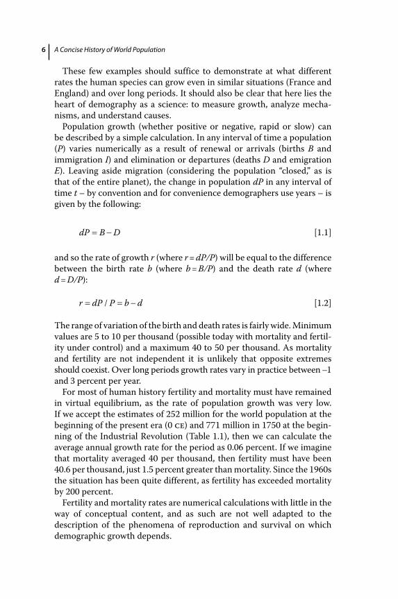
These few examples should suffice to demonstrate at what different rates the human species can grow even in similar situations (France and England) and over long periods. It should also be clear that here lies the heart of demography as a science: to measure growth, analyze mechanisms, and understand causes.
Population growth (whether positive or negative, rapid or slow) can be described by a simple calculation. In any interval of time a population (P) varies numerically as a result of renewal or arrivals (births B and immigration I) and elimination or departures (deaths D and emigration E). Leaving aside migration (considering the population “closed,” as is that of the entire planet), the change in population dP in any interval of time t – by convention and for convenience demographers use years – is given by the following:
dP B D [1.1]
and so the rate of growth r (where r = dP/P) will be equal to the difference between the birth rate b (where b = B/P) and the death rate d (where d = D/P):
r dP P b d/ [1.2]
The range of variation of the birth and death rates is fairly wide. Minimum values are 5 to 10 per thousand (possible today with mortality and fertility under control) and a maximum 40 to 50 per thousand. As mortality and fertility are not independent it is unlikely that opposite extremes should coexist. Over long periods growth rates vary in practice between –1 and 3 percent per year.
For most of human history fertility and mortality must have remained in virtual equilibrium, as the rate of population growth was very low. If we accept the estimates of 252 million for the world population at the beginning of the present era (0 ce) and 771 million in 1750 at the beginning of the Industrial Revolution (Table 1.1), then we can calculate the average annual growth rate for the period as 0.06 percent. If we imagine that mortality averaged 40 per thousand, then fertility must have been 40.6 per thousand, just 1.5 percent greater than mortality. Since the 1960s the situation has been quite different, as fertility has exceeded mortality by 200 percent.
Fertility and mortality rates are numerical calculations with little in the way of conceptual content, and as such are not well adapted to the description of the phenomena of reproduction and survival on which demographic growth depends.
The Space and Strategy of Demographic Growth 7
1.3 Jacopo Bichi and Domenica Del Buono, Jean Guyon, and Mathurine Robin
Jacopo Bichi was a humble sharecropper from Fiesole (near Florence).8 On November 12, 1667 he married Domenica Del Buono. Their marriage, although soon ended by the death of Jacopo, nonetheless produced three children: Andrea, Filippo, and Maria Maddalena. The latter died when only a few months old, but Andrea and Filippo survived and married. In a sense, Jacopo and Domenica paid off their demographic debt: the care received from their parents, and their own resistance and luck, succeeded in bringing them to reproductive age. They in turn bore and raised two children who also arrived at the same stage of maturity (reproductive age and marriage) and who, in a sense, replaced them exactly in the generational chain of life. Continuing the story of this family, Andrea married Caterina Fossi, and together they had four children, two of whom wed. Andrea and Caterina also paid their debt. Such was not the case for Filippo, who married Maddalena Cari. Maddalena died shortly afterward, having borne a daughter who in turn died at a young age. The two surviving sons of Andrea constitute the third generation: Giovan Battista married Caterina Angiola and had six children, all but one of whom died before marrying. Jacopo married Rosa, who bore eight children, four of whom married. Let us stop here and summarize the results of these five weddings (and 10 spouses):
Two couples (Jacopo and Domenica, Andrea and Caterina) paid their debt, each couple bringing two children to matrimony.
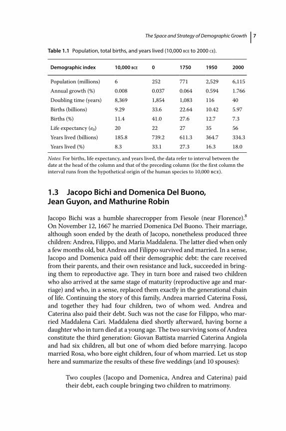
Table 1.1 Population, total births, and years lived (10,000 bce to 2000 ce).
Demographic index 10,000 bce 0 1750 1950 2000
Population (millions) 6 252 771 2,529 6,115Annual growth (%) 0.008 0.037 0.064 0.594 1.766Doubling time (years) 8,369 1,854 1,083 116 40Births (billions) 9.29 33.6 22.64 10.42 5.97Births (%) 11.4 41.0 27.6 12.7 7.3Life expectancy (e0) 20 22 27 35 56Years lived (billions) 185.8 739.2 611.3 364.7 334.3Years lived (%) 8.3 33.1 27.3 16.3 18.0
Notes: For births, life expectancy, and years lived, the data refer to interval between the date at the head of the column and that of the preceding column (for the first column the interval runs from the hypothetical origin of the human species to 10,000 bce).
A Concise History of World Population 8
One couple (Jacopo and Rosa) paid their debt with interest, as the two of them produced four wedded offspring.
One couple (Giovan Battista and Caterina Angiola) finished partially in debt in spite of the fact that they produced six children; only one wed.
One couple (Filippo and Maddalena) was completely insolvent, as no offspring survived to marry.
In three generations, five couples (10 spouses) produced nine wedded children in all. In biological terms, 10 breeders brought nine offspring to the reproductive phase, a 10 percent decline which, if repeated for an extended period, would lead to the family’s extinction.
A population, however, is made up of many families and many histories, each different from the others. In this same period, and applying the same logic, six couples of the Patriarchi family married off 15 children, while five Palagi couples did so with 10. The Patriarchi paid with interest, while the Palagi just fulfilled their obligation. The combination of these individual experiences, whether the balance is positive, negative, or even, determines the growth, decline, or stagnation of a population in the long run.
In 1608 Québec was founded and the French inhabitation of the St Lawrence Valley, virtually abandoned by the Iroquois, began.9 During the following century, approximately 15,000 immigrants arrived in these virgin lands from Normandy, from the area around Paris, and from central western France. Two‐thirds of these returned to France after stays of varying lengths. The current population of over 7 million French Canadians descends, for the most part, from those 5,000 immigrants who remained, as subsequent immigration contributed little to population growth. Thanks to a genealogic‐demographic reconstruction carried out by a group of Canadian scholars, a considerable amount of information relating to demographic events is known about this population. For example, two pioneers, Jean Guyon and Mathurine Robin, had 2,150 descendants by 1730. Naturally, subsequent generations, including wives and husbands from other genealogical lines, contributed to this figure, which in and of itself has little demographic significance. On the other hand, the fate of another pioneer, the famous explorer Samuel de Champlain, was very different, and he left no descendants at all. The extraordinary Canadian material also provides measures of significant demographic interest. For example, the 905 pioneers (men and women) who were born in France, migrated to Canada before 1660, and both married and died in Canada, produced on average 4.2 married offspring per couple (Figure 1.3), a level of fertility that corresponds to a doubling of the original population in a single generation (from two spouses, four married children). The exceptionally high reproductive capacity of the
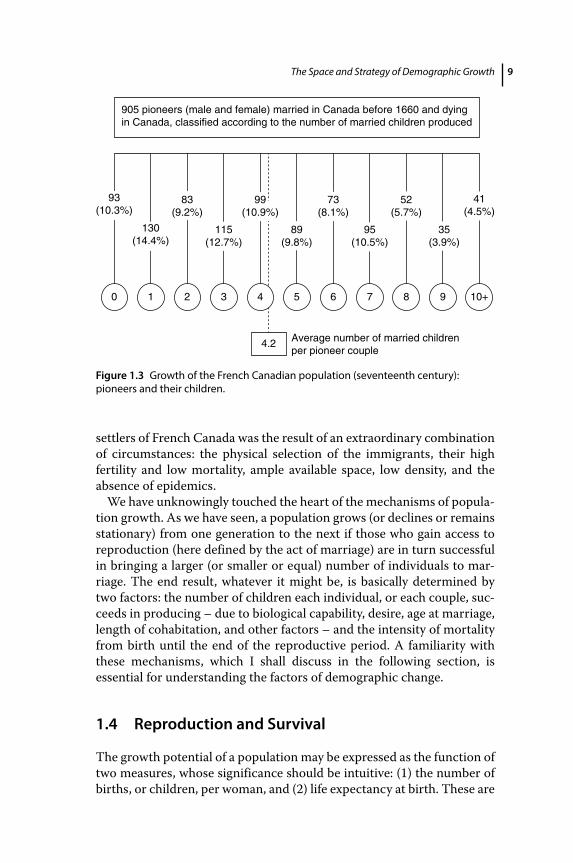
The Space and Strategy of Demographic Growth 9
settlers of French Canada was the result of an extraordinary combination of circumstances: the physical selection of the immigrants, their high fertility and low mortality, ample available space, low density, and the absence of epidemics.
We have unknowingly touched the heart of the mechanisms of population growth. As we have seen, a population grows (or declines or remains stationary) from one generation to the next if those who gain access to reproduction (here defined by the act of marriage) are in turn successful in bringing a larger (or smaller or equal) number of individuals to marriage. The end result, whatever it might be, is basically determined by two factors: the number of children each individual, or each couple, succeeds in producing – due to biological capability, desire, age at marriage, length of cohabitation, and other factors – and the intensity of mortality from birth until the end of the reproductive period. A familiarity with these mechanisms, which I shall discuss in the following section, is essential for understanding the factors of demographic change.
1.4 Reproduction and Survival
The growth potential of a population may be expressed as the function of two measures, whose significance should be intuitive: (1) the number of births, or children, per woman, and (2) life expectancy at birth. These are
905 pioneers (male and female) married in Canada before 1660 and dyingin Canada, classified according to the number of married children produced
Average number of married childrenper pioneer couple
4.2
0 1
130(14.4%)
115(12.7%)
89(9.8%)
95(10.5%)
35(3.9%)
41(4.5%)
52(5.7%)
73(8.1%)
83(9.2%)
93(10.3%)
2 3 4 5 6 7 8 9 10+
99(10.9%)
Figure 1.3 Growth of the French Canadian population (seventeenth century): pioneers and their children.
A Concise History of World Population 10
synthetic measures of, respectively, reproduction and survival. The first describes the average number of children produced by a generation of women during the course of their reproductive lives and in the hypothetical absence of mortality.10 In the following we consider the biological, social, and cultural factors that determine the level of this measure. The second, life expectancy at birth, describes the average duration of life (or average number of years lived) for a generation of newborns and is a function of the force of mortality at the various ages, which in turn is determined by the species’ biological characteristics and relationship with the surrounding environment. In the primarily rural societies of past centuries, which lacked modern birth control and effective medical knowledge, both of these measures might vary considerably. The number of children per woman ranged from less than five to more than eight (though today, in some western societies characterized by high levels of birth control, it has declined below one), and life expectancy at birth ranged from 20 to 40 years (today it has exceeded 80 in some countries).
The number of children per woman depends, as has been said, on biological and social factors that determine: (1) the frequency of births during a woman’s fecund period, and (2) the portion of the fecund period – between puberty and menopause – effectively utilized for reproduction.11
1.4.1 The frequency of births
This is an inverse function of the interval between births. Given the condition of natural fertility – a term used by demographers to describe those premodern societies that did not practice intentional contraception for the purpose of controlling either the number of births or their timing – the interval between births may be divided into four parts:
1) A period of infertility after every birth, as ovulation does not recommence for a couple of months. However, this anovulatory period, during which it is impossible to conceive, increases with the duration of breast‐feeding, which is often continued until the second, and in some cases even third, year of the child’s life. The duration of breast‐feeding, however, varies considerably from one culture to another, so much so that the minimum and maximum limits for the infertility period fall between 3 and 24 months.
2) The waiting time, that is, the average number of months that pass between the resumption of normal ovulation and conception. It is possible that some women, either for accidental or natural reasons, may conceive during the first ovulatory cycle, while others, even given regular sexual relations, may not do so for many cycles. We can take 5 and 10 months as our upper and lower limits.
The Space and Strategy of Demographic Growth 11
3) The average length of pregnancy, which as everyone knows is about 9 months.
4) Fetal mortality. About one out of every five recognized pregnancies does not come to term because of miscarriage. According to the few studies available, this seems to be a frequency that does not vary much from population to population. After a miscarriage, a new conception can take place after the normal waiting period (5 to 10 months). As only one in five conceptions contributes to this component of the birth interval, the average addition is 1–2 months.
Totaling the minimum and maximum values of 1, 2, 3, and 4, we find that the interval between births ranges from 18 to 45 months (or approximately 1.5 to 3.5 years), but, as a combination either of maxima or minima is improbable, this interval usually falls between 2 and 3 years. The above analysis holds true for a population characterized by uncontrolled, natural fertility. Of course, if birth control is introduced the reproductive life span without children may be expanded at will.
1.4.2 The fecund period used for reproduction
The factors that determine the age of access to reproduction, or the establishment of a stable union for the purpose of reproduction (marriage), are primarily cultural, while those that determine the age at which the reproductive period ends are primarily biological.
1) The age at marriage may vary between a minimum close to the age of puberty – let us say 15 years – and a maximum that in many European societies has exceeded 25.
2) The age at the end of the fecund period may be as high as 50, but on average is much lower. We can take as a good indicator the average age of mothers at the birth of the last child in populations that do not practice birth control. This figure is fairly stable and varies between 38 and 41.
We can say, then – again combining minima and maxima and rounding – that the average length of a union for reproductive purposes, barring death or divorce, may vary between 15 and 25 years.
Simplifying still more, we can estimate what the minimum and maximum levels of procreation might be in hypothetical populations not subject to mortality. To obtain the minimum we combine the minimum reproductive period (15 years) with the maximum birth interval (3.5 years).
15
3 54 3year reproductive period
year birth intervalchild
.. rren
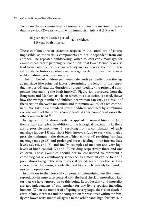
A Concise History of World Population 12
To obtain the maximum level we instead combine the maximum reproductive period (25 years) with the minimum birth interval (1.5 years):
251 5
16 7year reproductive periodyear birth interval
chil.
. ddren
These combinations of extremes (especially the latter) are of course impossible, as the various components are not independent from one another. The repeated childbearing, which follows early marriage, for example, can create pathological conditions that lower fecundity or else lead to an early decline in sexual activity and so increase the birth interval. In stable historical situations, average levels of under five or over eight children per woman are rare.
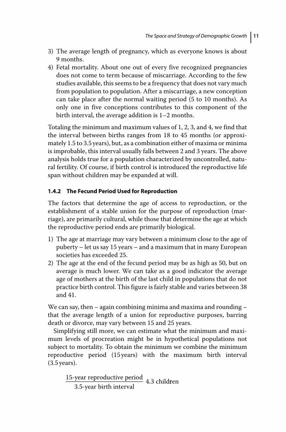
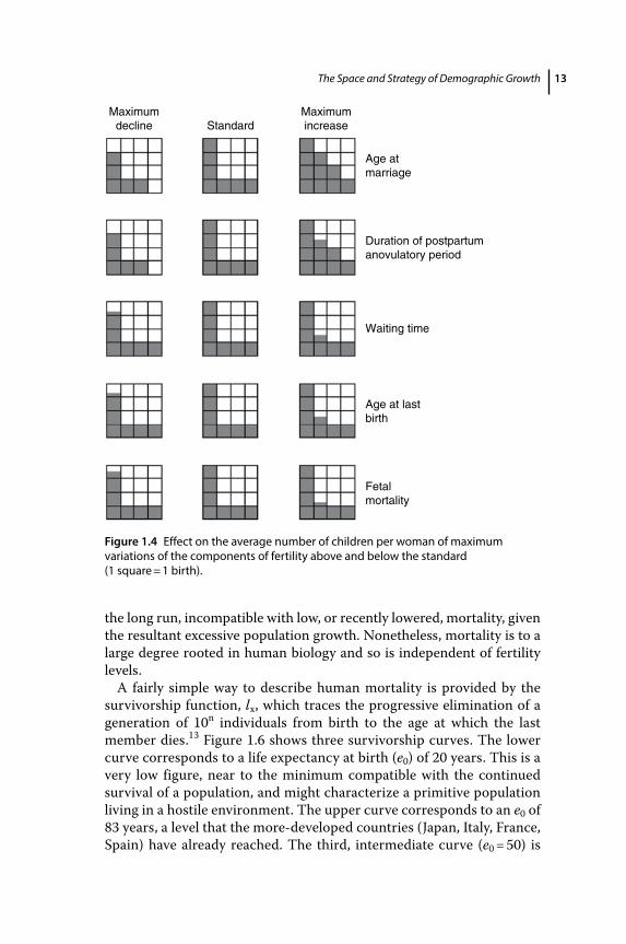
The number of children per woman depends primarily upon the age at marriage (the principal factor determining the length of the reproductive period) and the duration of breast‐feeding (the principal component determining the birth interval). Figure 1.4, borrowed from the Bongaarts and Menken article on which this discussion is based, shows how the average number of children per woman can vary as a result of the variation (between maximum and minimum values) of each component. We take as a standard seven children, obtained by combining average values of the various components. As one component varies the others remain fixed.12
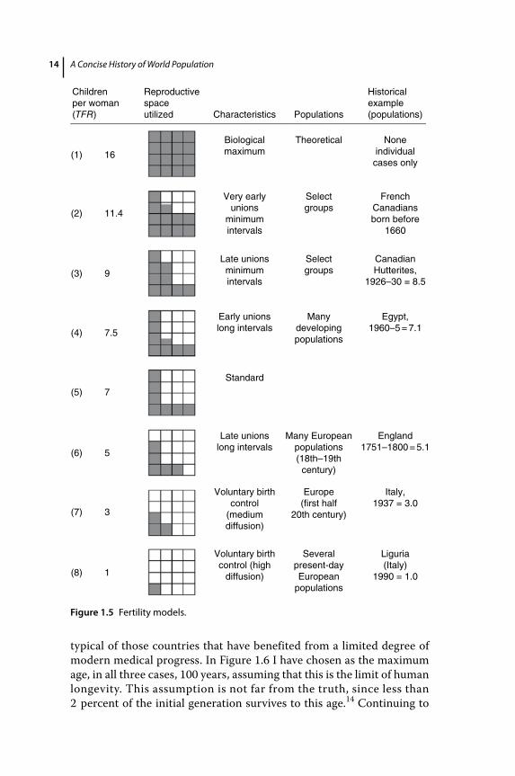
In Figure 1.5 the above model is applied to several historical (and theoretical) examples. In addition to the biological maximum (1), there are: a possible maximum (2) resulting from a combination of early marriage (at age 18) and short birth intervals (due to early weaning); a possible minimum in the absence of birth control (6) resulting from late marriage (at age 25) and prolonged breast‐feeding; three intermediate levels (3), (4), and (5); and finally, examples of medium and very high levels of birth control, (7) and (8), yielding respectively three and one children. These examples should not be considered to represent a chronological or evolutionary sequence, as almost all can be found in populations living in the same historical periods (except for the last two, characterized by strongly controlled fertility, which can only be found in modern populations).
In addition to the biosocial components determining fertility, human reproductivity must also contend with the hard check of mortality, a factor that we have ignored up to this point. Reproductivity and mortality are not independent of one another for any living species, including humans. When the number of offspring is very large, the risk of death in early infancy increases and the competition for resources within the family can lower resistance at all ages. On the other hand, high fertility is, in
The Space and Strategy of Demographic Growth 13
the long run, incompatible with low, or recently lowered, mortality, given the resultant excessive population growth. Nonetheless, mortality is to a large degree rooted in human biology and so is independent of fertility levels.
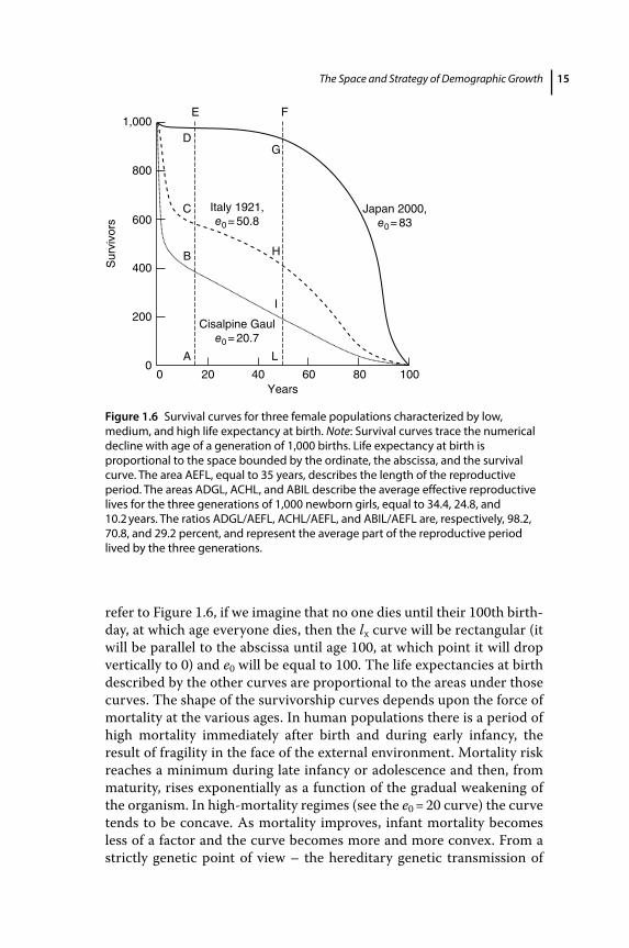
A fairly simple way to describe human mortality is provided by the survivorship function, lx, which traces the progressive elimination of a generation of 10n individuals from birth to the age at which the last member dies.13 Figure 1.6 shows three survivorship curves. The lower curve corresponds to a life expectancy at birth (e0) of 20 years. This is a very low figure, near to the minimum compatible with the continued survival of a population, and might characterize a primitive population living in a hostile environment. The upper curve corresponds to an e0 of 83 years, a level that the more‐developed countries (Japan, Italy, France, Spain) have already reached. The third, intermediate curve (e0 = 50) is
Maximumdecline Standard
Maximumincrease
Age atmarriage
Waiting time
Age at lastbirth
Fetalmortality
Duration of postpartumanovulatory period
Figure 1.4 Effect on the average number of children per woman of maximum variations of the components of fertility above and below the standard (1 square = 1 birth).
A Concise History of World Population 14
typical of those countries that have benefited from a limited degree of modern medical progress. In Figure 1.6 I have chosen as the maximum age, in all three cases, 100 years, assuming that this is the limit of human longevity. This assumption is not far from the truth, since less than 2 percent of the initial generation survives to this age.14 Continuing to
Childrenper woman(TFR)
Reproductivespaceutilized Characteristics Populations
Theoretical Noneindividualcases only
Biologicalmaximum(1) 16
(2) 11.4
(3) 9
(4) 7.5
(5) 7
(6) 5
(7) 3
(8) 1
Very earlyunions
minimumintervals
FrenchCanadiansborn before
1660
Selectgroups
Selectgroups
CanadianHutterites,
1926–30 = 8.5
Early unionslong intervals
Standard
Severalpresent-dayEuropean
populations
Liguria(Italy)
1990 = 1.0
Voluntary birthcontrol (high
diffusion)
Italy,1937 = 3.0
Europe(first half
20th century)
Voluntary birthcontrol
(mediumdiffusion)
England1751–1800 = 5.1
Many Europeanpopulations(18th–19th
century)
Late unionslong intervals
Egypt,1960–5 = 7.1
Manydevelopingpopulations
Late unionsminimumintervals
Historicalexample(populations)
Figure 1.5 Fertility models.
The Space and Strategy of Demographic Growth 15
refer to Figure 1.6, if we imagine that no one dies until their 100th birthday, at which age everyone dies, then the lx curve will be rectangular (it will be parallel to the abscissa until age 100, at which point it will drop vertically to 0) and e0 will be equal to 100. The life expectancies at birth described by the other curves are proportional to the areas under those curves. The shape of the survivorship curves depends upon the force of mortality at the various ages. In human populations there is a period of high mortality immediately after birth and during early infancy, the result of fragility in the face of the external environment. Mortality risk reaches a minimum during late infancy or adolescence and then, from maturity, rises exponentially as a function of the gradual weakening of the organism. In high‐mortality regimes (see the e0 = 20 curve) the curve tends to be concave. As mortality improves, infant mortality becomes less of a factor and the curve becomes more and more convex. From a strictly genetic point of view – the hereditary genetic transmission of
00
200
400
600
Sur
vivo
rs
800
1,000
20 40
Cisalpine Gaule0= 20.7
Italy 1921,e0= 50.8
Japan 2000,e0= 83
A L
GD
E F
C
B H
I
60Years
80 100
Figure 1.6 Survival curves for three female populations characterized by low, medium, and high life expectancy at birth. Note: Survival curves trace the numerical decline with age of a generation of 1,000 births. Life expectancy at birth is proportional to the space bounded by the ordinate, the abscissa, and the survival curve. The area AEFL, equal to 35 years, describes the length of the reproductive period. The areas ADGL, ACHL, and ABIL describe the average effective reproductive lives for the three generations of 1,000 newborn girls, equal to 34.4, 24.8, and 10.2 years. The ratios ADGL/AEFL, ACHL/AEFL, and ABIL/AEFL are, respectively, 98.2, 70.8, and 29.2 percent, and represent the average part of the reproductive period lived by the three generations.
A Concise History of World Population 16
characteristics – survival beyond the reproductive years (for simplicity, say 50 years of age) is of course irrelevant. However high or low it might be, the rate of mortality beyond age 50 will have no effect on the genetic patrimony of a population. Before and during the reproductive years, on the other hand, the higher the level of mortality, the stronger the selective effect, as individuals possessing characteristics unfavorable to survival are eliminated and so do not pass on these characteristics to subsequent generations.
Nonetheless, increased survival beyond the reproductive ages may have indirect biological effects, as older adults contribute to the accumulation, organization, and transmission of knowledge, while also favoring parental investments, and so can contribute to the improved survival of new generations.
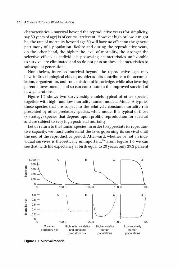
Figure 1.7 shows two survivorship models typical of other species, together with high‐ and low‐mortality human models. Model A typifies those species that are subject to the relatively constant mortality risk presented by other predatory species, while model B is typical of those (r‐strategy) species that depend upon prolific reproduction for survival and are subject to very high postnatal mortality.
Let us return to the human species. In order to appreciate its reproductive capacity, we must understand the laws governing its survival until the end of the reproductive period. Afterward, whether or not an individual survives is theoretically unimportant.15 From Figure 1.6 we can see that, with life expectancy at birth equal to 20 years, only 29.2 percent
0
0.2
0.4
Mor
talit
y ris
kS
urvi
vors
0.6
0.8
1.0
00 100 100 0 100 0 1000
0 100
Constantpredatory risk
High initial mortalityand constantpredatory risk
High-mortalityhuman
populations
Low-mortalityhuman
populations
100 0 100 0 1000
200
400
600
800
1,000 A B C D
A B C D
Figure 1.7 Survival models.
The Space and Strategy of Demographic Growth 17
of the potential fecund life of a generation is actually lived owing to the decimation caused by high mortality. This proportion increases gradually with increasing life expectancy (and the elevation of the lx curve). In the examples given, it is 70.8 percent when e0 equals 50 and 98.2 percent when e0 equals 83.
It should be clear now that the reproductive success of a population – and so its growth – depends upon the number of children born to those women who survive to reproductive age. If we imagine a level of six children per woman in the absence of mortality, then in that case where only 30 percent of the reproductive space is used (e0 = 20) the number of children born per woman is 6 × 0.3 = 1.8. When e0 = 50 and 70 percent of the reproductive space is used, the number of children is 6 × 0.7 = 4.2; and when 99 percent is used (e0 = 83), the total is 6 × 0.99 = 5.94. Since there are two parents for every child, each hypothetical couple pays its demographic debt (and the number of parents and children is about equal) if our calculation above yields a level of two. A number larger than two implies growth. If the number of surviving children is four, then the population will double in the course of a single generation (about 30 years) and the average annual growth rate will be 2.3 percent.16
1.5 The Space of Growth
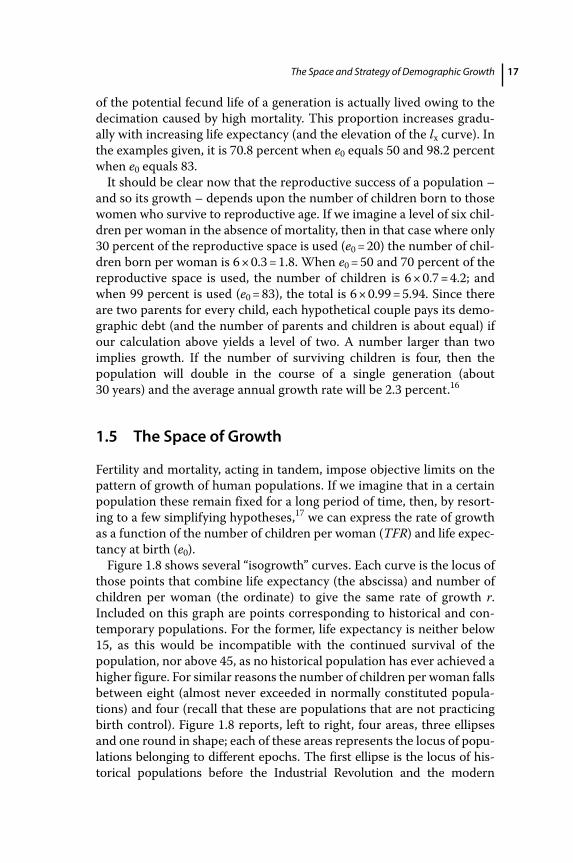
Fertility and mortality, acting in tandem, impose objective limits on the pattern of growth of human populations. If we imagine that in a certain population these remain fixed for a long period of time, then, by resorting to a few simplifying hypotheses,17 we can express the rate of growth as a function of the number of children per woman (TFR) and life expectancy at birth (e0).
Figure 1.8 shows several “isogrowth” curves. Each curve is the locus of those points that combine life expectancy (the abscissa) and number of children per woman (the ordinate) to give the same rate of growth r. Included on this graph are points corresponding to historical and contemporary populations. For the former, life expectancy is neither below 15, as this would be incompatible with the continued survival of the population, nor above 45, as no historical population has ever achieved a higher figure. For similar reasons the number of children per woman falls between eight (almost never exceeded in normally constituted populations) and four (recall that these are populations that are not practicing birth control). Figure 1.8 reports, left to right, four areas, three ellipses and one round in shape; each of these areas represents the locus of populations belonging to different epochs. The first ellipse is the locus of historical populations before the Industrial Revolution and the modern
A Concise History of World Population 18
diffusion of birth control. These populations fall within a band of growth rates that extends from 0 to 1 percent, a space of growth typical of premodern times. Within this narrow band, however, the fertility and mortality combinations vary widely, although constrained by the syndromic poverty of resources and of knowledge. Denmark at the end of the eighteenth century and India a century later, for example, have similar growth rates, but these are achieved at distant points in the strategic space described: the former example combines high life expectancy (about 40 years) and a small number of children (just over four), while in the latter case low life expectancy (about 25 years) is paired with many children (just under seven).
Although their growth rates must have been similar, the points for Paleolithic and Neolithic populations are assumed to have been far apart. According to a well‐accepted opinion (see Chapter 2), the Paleolithic, a hunting and gathering population, was characterized by lower mortality, owing to its low density, a factor that prevented infectious diseases from taking hold and spreading, and moderate fertility, compatible with its nomadic behavior. For the Neolithic, a sedentary and agricultural population, both mortality and fertility were higher as a result of higher density and lower mobility.
The second ellipse contains the populations during the process of demographic transition in the twentieth century. The strategic space utilized, previously restricted to a narrow band, has expanded dramatically. Medical and sanitary progress has shifted the upper limit of life expectancy from the historical level of about 40 years to the present level of
200
1
2
3
4
5
Chi
ldre
n pe
r w
oman
(TE
R)
6
7
8
9
10
30
r = 1%
r = 3%
40 50
Pre modempopulations
Future?
Life expectancy (E0)
60 70 80
Populations in transition beginningXXI century
Populations intransition, XX century
r = 0%
r = –1%
Figure 1.8 Relationship between the average number of children per woman (TFR) and life expectancy (e0) in historical and present‐day populations.
The Space and Strategy of Demographic Growth 19
above 80 years, while the introduction of birth control has reduced the lower limit of fertility to a level of about one child per woman. The third ellipse outlines the situation at the beginning of the twenty‐first century, when countries with very high fertility (many in sub‐Saharan Africa) coexist with other countries (in Europe and Southern and Eastern Asia) with abnormally low fertility, close to one child per woman. It must be remarked that in the much expanded space of the twentieth and twenty‐first centuries there are populations with implicit growth rates of 4 percent, and other populations with negative growth rates of −2 percent. A population with a 4 percent rate of growth doubles in 17–18 years, and one declining at the rate of 2 percent halves in 35 years.18 Two populations of equal size experiencing these different growth rates will find themselves after 35 years (about a generation) in a numerical ratio of 8:1! However, this is the space of populations in transition, unstable, and often with unsustainable paces of growth. The fourth space, circular in shape, is the hypothetical region of the future, after the transition and at the end of a process of convergence, with an expectation of life above 80, fertility between 1 and 3 children per woman, and potential rates of growth between −1 and +1 percent. These populations could alternate phases of growth and decline, possibly not synchronized, with relatively small and diluted changes in time.
1.6 Environmental Constraints
Although the strategic space of growth is large, only a small portion of it can be permanently occupied by a population. Sustained decline is obviously incompatible with the survival of a human group, while sustained growth can in the long run be incompatible with the resources available. The mechanisms of growth, therefore, must continually adjust to environmental conditions (which we might call environmental friction), conditions with which they interact but which also present obstacles to growth, as attested to by the millennia during which the population growth rate has been very low. For the moment I shall limit myself to the macroscopic aspects of these obstacles to demographic growth, saving for later a more detailed discussion of their operation.
In a justly famous essay, Carlo Cipolla wrote: “It is safe to say that until the Industrial Revolution man continued to rely mainly on plants and animals for energy – plants for food and fuel, and animals for food and mechanical energy.”19 It is this subordination to the natural environment and the resources it provides that constituted a check to population increase, a situation particularly evident for a hunting and gathering society. Imagine a population that utilizes a habitat
A Concise History of World Population 20
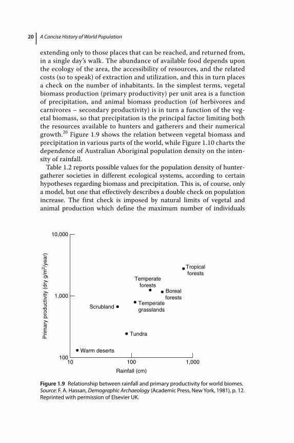
extending only to those places that can be reached, and returned from, in a single day’s walk. The abundance of available food depends upon the ecology of the area, the accessibility of resources, and the related costs (so to speak) of extraction and utilization, and this in turn places a check on the number of inhabitants. In the simplest terms, vegetal biomass production (primary productivity) per unit area is a function of precipitation, and animal biomass production (of herbivores and carnivores – secondary productivity) is in turn a function of the vegetal biomass, so that precipitation is the principal factor limiting both the resources available to hunters and gatherers and their numerical growth.20 Figure 1.9 shows the relation between vegetal biomass and precipitation in various parts of the world, while Figure 1.10 charts the dependence of Australian Aboriginal population density on the intensity of rainfall.
Table 1.2 reports possible values for the population density of hunter‐gatherer societies in different ecological systems, according to certain hypotheses regarding biomass and precipitation. This is, of course, only a model, but one that effectively describes a double check on population increase. The first check is imposed by natural limits of vegetal and animal production which define the maximum number of individuals
10100
1,000
Prim
ary
prod
uctiv
ity (
dry
g/m
2 /ye
ar)
10,000
100
Rainfall (cm)
1,000
Tundra
Warm deserts
Scrubland
Temperateforests
Temperategrasslands
Borealforests
Tropicalforests
Figure 1.9 Relationship between rainfall and primary productivity for world biomes. Source: F. A. Hassan, Demographic Archaeology (Academic Press, New York, 1981), p. 12. Reprinted with permission of Elsevier UK.
The Space and Strategy of Demographic Growth 21
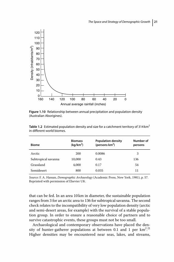
that can be fed. In an area 10 km in diameter, the sustainable population ranges from 3 for an arctic area to 136 for subtropical savanna. The second check relates to the incompatibility of very low population density (arctic and semi‐desert areas, for example) with the survival of a stable population group. In order to ensure a reasonable choice of partners and to survive catastrophic events, these groups must not be too small.
Archaeological and contemporary observations have placed the density of hunter‐gatherer populations at between 0.1 and 1 per km2.21 Higher densities may be encountered near seas, lakes, and streams,
1600
10
20
30
40
50
60
Den
sity
(in
habi
tant
s/m
2 )
70
80
90
100
110
120
140 120 100
Annual average rainfall (inches)
80 60 40 20 0
Figure 1.10 Relationship between annual precipitation and population density (Australian Aborigines).
Table 1.2 Estimated population density and size for a catchment territory of 314 km2 in different world biomes.
BiomeBiomass (kg/km2)
Population density (persons km2)
Number of persons
Arctic 200 0.0086 3Subtropical savanna 10,000 0.43 136Grassland 4,000 0.17 54Semidesert 800 0.035 11
Source: F. A. Hassan, Demographic Archaeology (Academic Press, New York, 1981), p. 57. Reprinted with permission of Elsevier UK.
A Concise History of World Population 22
where fishing can effectively supplement the products of the earth. Clearly the limiting factors at this cultural level are essentially precipitation and the availability and accessibility of land.
The Neolithic transition to stable cultivation of the land and the raising of livestock certainly represented a dramatic expansion of productive capacity. This transition, which many call a “revolution,” developed and spread slowly over millennia in a variety of ways and forms. The progress of cultivation techniques, from slash and burn to triannual rotations (which have coexisted in different cultures up to the present day); the selection of better and better seeds; the domestication of new plants and animals; and the use of animal, air, and water power have all enormously increased the availability of food and energy.22 Population density as a result also grew; that of major European countries (France, Italy, Germany, England, the Low Countries) in the mid‐eighteenth century was about 40–60 persons per km2, 100 times greater than that of the hunters and gatherers. Naturally, productive capacity varied greatly in different epochs as a function of technological and social evolution, a point easily demonstrated by comparing the agriculture of the Po Valley or the Low Countries with the fairly primitive methods used in some parts of the continent. Throughout the globe, innovation has allowed for the notable expansion of productivity per unit of energy invested. It appears, for example, that productivity per hectare tripled in Teotihuacán (Mexico) between the third and second millennia bce due to the introduction of new varieties of corn;23 and in various zones of Europe during the modern era the ratio of agricultural production to seed increased thanks to new grains.24
Nonetheless, success in mastering the environment has always been dependent upon the availability of energy. As Cipolla observed, “the fact that the main sources of energy other than man’s muscular work remained basically plants and animals must have set a limit to the possible expansion of the energy supply in any given agricultural society of the past. The limiting factor in this regard is ultimately the supply of land.”25 In preindustrial Europe, populations seem to have approached with some frequency the limits allowed by the environment and available technology. These limits may be expressed by the per capita availability of energy and, again following Cipolla, must have been below 15,000 calories, or perhaps even 10,000, per day (a level which the richest countries today exceed by a factor of 20 or 30), the majority of which were dedicated to nutrition and heating.26
The environmental limits to demographic expansion were again shattered by the enormous increase in available energy that resulted from the industrial and technological revolution of the second half of the eighteenth century and the invention of efficient machines for the conversion
The Space and Strategy of Demographic Growth 23
of inanimate materials into energy. World production of coal increased 10‐fold between 1820 and 1860 and again between 1860 and 1950. It has been calculated that worldwide primary energy consumption almost tripled between 1800 and 1900, and increased ninefold between 1900 and 2000, and that per capita consumption expanded fourfold during the past two centuries, moving from a state of penury to one of relative abundance.27 The dependency of energy availability on land availability was again (and perhaps definitively) broken and the principal obstacle to the numerical growth of population removed. A synthesis of this complex development has been made by Earl Cook: hunters and gatherers needed some 5,000 calories per capita and per day; agriculturalists probably never exceeded a consumption level of 12,000 calories; and before the Industrial Revolution even the most developed and structured populations’ consumption remained below 26,000 calories. In the initial phase of the Industrial Revolution per capita consumption – derived mostly from fossil fuels – was of the order of 70,000 calories, while it exceeds 200,000 in some contemporary societies.28
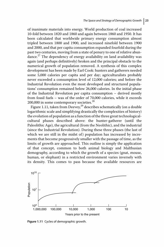
Figure 1.11, taken from Deevey,29 describes schematically (on a double logarithmic scale and simplifying drastically the complexities of history) the evolution of population as a function of the three great technological‐ cultural phases described above: the hunter‐gatherer (until the Paleolithic Age), the agricultural (from the Neolithic), and the industrial (since the Industrial Revolution). During these three phases (the last of which we are still in the midst of ) population has increased by increments that become progressively smaller with the passage of time, as the limits of growth are approached. This outline is simply the application of that concept, common to both animal biology and Malthusian demography, according to which the growth of a species (gnat, mouse, human, or elephant) in a restricted environment varies inversely with its density. This comes to pass because the available resources are
1,000,000
Pop
ulat
ion
104
107
1010
100,000 10,000
Years prior to the present
1,000 100 10
Figure 1.11 Cycles of demographic growth.
A Concise History of World Population 24
considered fixed and so population growth creates its own checks. For the human species, of course, the environment, and so the available resources, has never been fixed but continually expands due to innovation. In the Deevey outline, demographic growth in the first long period of human history, which continued up until 10,000 years ago, was limited by the biomass available for nutrition and heating at a rate of several thousand calories per day per person. In the second phase, from the Neolithic to the Industrial Revolution, limits were imposed by the availability of land and the limited energy provided by plants, animals, water, and wind. In the present phase, the limits to growth are not so well defined, but may be connected to the adverse environmental effects of combined demographic and technological growth and the attendant cultural choices.
1.7 A Few Figures
On November 1, 2010, the People’s Republic of China carried out its sixth census since the revolution and, with the help of 10 million carefully trained census personnel, counted 1.340 billion inhabitants. It was the largest social investigation ever undertaken. Until the middle of the twentieth century there were still quite a few areas of the less‐developed world for which there existed, at best, fragmentary and incomplete demographic estimates. In western countries the modern statistical era began in the nineteenth century, when the practice of taking censuses of the population at regular intervals, begun by some countries in the preceding century, became general. The 10.4 million persons counted in the Kingdom of Spain in the summer of 1787 by order of Charles III’s prime minister, Floridablanca, and the 3.9 million counted in the United States in 1790 as instructed by the first article of the Constitution approved 3 years earlier in Philadelphia, are the first examples of modern censuses in large countries.30 In previous centuries there were, of course, head counts and estimates – often serving fiscal purposes – for limited areas and often of limited coverage. Included among the latter are the family lists from the Han to the Ching dynasties in China (covering a period of almost two millennia ending in the previous century).31 For the evaluation of these the work of the statistician must be complemented by that of the historian, who is able to evaluate, integrate, and interpret the sources. In many parts of the world before this century, in Europe prior to the late Middle Ages or in China before the present era, one can only estimate population size on the basis of qualitative information – the existence or extension of cities, villages, or other settlements, the extension of cultivated land – or on the basis of calculations of the possible
The Space and Strategy of Demographic Growth 25
population density in relation to the ecosystem, the level of technology, or social organization. The contributions of paleontologists, archaeologists, and anthropologists are all needed.
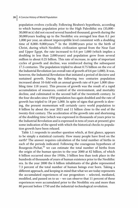
The data on world demographic growth, as in Table 1.1 and Table 1.3, are largely based on conjectures and inferences drawn from nonquantitative information. Table 1.1 presents a synthesis of these trends. The long‐term rates of growth are, of course, an abstraction, as they imply a constant variation of demographic forces in each period, while in reality
Table 1.3 Continental populations (400 bce to 2050 ce, millions).
Year Asia Europe Africa America Oceania World
400 bce 97 30 17 8 1 1530 172 41 26 12 1 252
200 160 55 30 11 1 257600 136 31 24 16 1 208
1000 154 41 39 18 1 2531200 260 64 48 26 2 4001340 240 88 80 32 2 4421400 203 63 68 39 2 3751500 247 82 87 42 3 4611600 341 108 113 13 3 5781700 437 121 107 12 3 6801750 505 141 104 18 3 7711800 638 188 102 24 2 9541850 801 277 102 59 2 1,2411900 92 404 138 165 6 1,6341950 1,403 547 224 332 13 2,52920002050
3,7145,267
726707
8142448
8411217
3157
6,1279,725
% rate of growth0–1750 0.06 0.07 0.08 0.02 0.06 0.061750–1950 0.51 0.68 0.38 1.46 0.73 0.591950–20002000–2050
1.950.70
0.57−0.05
2.582.20
1.860.74
1.741.22
1.770.92
Sources: J. N. Biraben, “Essai sur L’évolution du Nombre des Hommes [Essay on the Evolution of the Population],” Population 34 (1979), p.16. For 1950 and 2000: United Nations, World Population Prospects: The 2015 Revision (New York, 2015).
A Concise History of World Population 26
population evolves cyclically. Following Biraben’s hypothesis, according to which human population prior to the High Paleolithic era (35,000–30,000 bce) did not exceed several hundred thousand, growth during the 30,000 years leading up to the Neolithic era averaged less than 0.1 per 1,000 per year, an almost imperceptible level consistent with a doubling time of 8,000–9,000 years.32 In the 10,000 years prior to the birth of Christ, during which Neolithic civilization spread from the Near East and Upper Egypt, the rate increased to 0.4 per 1,000 (which implies a doubling in less than 2,000 years) and population grew from several million to about 0.25 billion. This rate of increase, in spite of important cycles of growth and decline, was reinforced during the subsequent 17.5 centuries. The population tripled to about 0.75 billion on the eve of the Industrial Revolution (an overall rate of growth of 0.6 per 1,000). It was, however, the Industrial Revolution that initiated a period of decisive and sustained growth. During the following two centuries population increased about 10‐fold with an annual growth rate of 6 per 1,000 (doubling time 118 years). This process of growth was the result of a rapid accumulation of resources, control of the environment, and mortality decline, and culminated in the second half of the twentieth century. In the four decades since 1950 population has again doubled and the rate of growth has tripled to 18 per 1,000. In spite of signs that growth is slowing, the present momentum will certainly carry world population to 8 billion by about the year 2023 and 11 billion close to the end of the twenty‐first century. The acceleration of the growth rate and shortening of the doubling time (which was expressed in thousands of years prior to the Industrial Revolution and is expressed in tens of years at present) give some indication of the speed with which the historical checks to population growth have been relaxed.
Table 1.1 responds to another question which, at first glance, appears to be simply a statistical curiosity. How many people have lived on the earth? The answer requires calculation of the total number of births in each of the periods indicated. Following the courageous hypotheses of Bourgeois‐Pichat,33 we can estimate the total number of births from the origin of the human species to the year 2000 at 82 billion, of which 6 billion occurred since the 1950s, 3 billion less than took place in the hundreds of thousands of years of human existence prior to the Neolithic era. In the year 2000 the 6 billion inhabitants of the globe represented 7.3 percent of the total number of human beings ever born. Taking a different approach, and keeping in mind that what we are today represents the accumulated experiences of our progenitors – selected, mediated, modified, and passed on to us – we can observe that 11 percent of these experiences were accumulated prior to the Neolithic era and more than 80 percent before 1750 and the industrial‐technological revolution.
The Space and Strategy of Demographic Growth 27
If we assign an estimated life expectancy at birth to the individuals in each epoch (these estimates are statistical only for the last period; for the preceding period they are based on fragmentary evidence and before that they are pure conjecture), we can then calculate the total number of years lived by each of these groups. Those born between 1950 and 2000 will have lived (at the end of their lives) about 334 billion years, almost twice the total number of years lived by all those born prior to the Neolithic era. The 420 billion years that will presumably be lived (during their whole lives) by those alive in 2000 represent a little less than one‐fifth of all the years lived since the origin of the human race. Finally, with a rather gross estimate, we may say that humankind’s energy consumption, during the past 13 years or so, has been of the same order of magnitude of the total energy consumption from 0 ce to the onset of the industrial revolution.34 These figures are not presented for their shock value, but to demonstrate the extraordinary expansion of resources available to humanity today as compared to earlier agricultural societies.
Population, of course, did not grow continuously, but experienced cycles of growth and decline, the long‐term aspects of which are summarized in Table 1.3 and Figure 1.11. Limiting ourselves to Europe, the tripling of population between the birth of Christ and the eighteenth century did not occur gradually, but was the result of successive waves of expansion and crisis: crisis during the late Roman Empire and the Justinian era as a result of barbarian invasions and disease; expansion in the twelfth and thirteenth centuries; crisis again as a result of recurring and devastating bouts of the plague beginning in the mid‐fourteenth century; a strong rallying from the mid‐fifteenth century to the end of the sixteenth century; and crisis or stagnation until the beginning of the eighteenth century, when the forces of modern expansion came to the fore. Nor do these cycles run parallel in different areas, so that relative demographic weight changes with time: the European share of world population grew from 17.8 to 24.7 percent between 1500 and 1900, only to decline again to 11.9 percent in the year 2000. The entire American continent contained about 2 percent of the world’s population at the beginning of the seventeenth century, while today the figure is 13.3 percent.
Notes
1 J. W. Goethe, Italian Journey, trans. W. H. Auden and E. Mayer (North Point Press, San Francisco, 1982), p. 46.
2 H. Cortés, Cartas de relación (Editorial Porrúa, Mexico, 1976), p. 62.3 For the discussion that follows I have taken the lead provided by R. M.
May and D. I. Rubinstein in their “Reproductive Strategies,” in C. R. Austin
A Concise History of World Population 28
and R. V. Short, eds., Reproductive Fitness (Cambridge University Press, London, 1984), pp. 1–23. See also R. V. Short, “Species Differences in Reproductive Mechanisms,” in the same volume, pp. 24–61. An essay of broader scope is that of S. C. Stearns, “Life History Tactics: a Review of the Ideas,” Quarterly Review of Biology 51 (1976). The relevance of r and K strategies to demography is supported by A. J. Coale in the first chapter of A. J. Coale and S. Cotts Watkins, eds., The Decline of Fertility in Europe (Princeton University Press, Princeton, NJ, 1986), p. 7.
4 May and Rubinstein, “Reproductive Strategies,” p. 2.5 May and Rubinstein, in “Reproductive Strategies,” note that for
mammals there exists a close relationship between body weight and age of sexual maturity. As we shall see below, the rate of growth of a population can be derived from Lotka’s equation, r = ln R0 / T, where T is the average length of generation and R0 is the average number of daughters a generation of women have during their lifetime (net reproduction rate). It follows that r is reasonably sensitive to changes in T (closely linked to the age of sexual maturity) and less sensitive to changes in R0, as it is directly linked to ln R0. Changes in the value of T, then, from species to species, have a strong influence on the value of r.
6 F. MacFarlane Burnet, Natural History of Infectious Diseases (Cambridge University Press, London, 1962), p. 14.
7 May and Rubinstein, “Reproductive Strategies,” p. 1.8 I am indebted to Carlo Corsini for having supplied me with the following
examples taken from family reconstructions for the diocese of Fiesole.9 The discussion that follows is derived from H. Charbonneau, Réal Bates
and Mario Boleda, Naissance d’une Population. Les Français Établis au Canada au XVII e Siècle [The Birth of a Population: The French Settlement in Canada in the XVIIth Century] (Presses de la Université de Montréal, Montréal, 1987).
10 The average number of children per woman, or total fertility rate (TFR), is the sum of age‐specific fertility rates for women between the minimum and maximum ages of reproduction, fx = Bx/PxBx is the number of births to a woman aged x, and Px is the female population age x.
11 The discussion that follows owes a heavy debt to the work of J. Bongaarts and J. Menken, “The Supply of Children: A Critical Essay,” in R. A. Bulatao and R. B. Lee, eds., Determinants of Fertility in Developing Countries (Academic Press, New York, 1983), vol. 1, pp. 27–60. The evaluation of the components of fertility is based on the assumption that all births are the products of stable unions (marriage), an hypothesis close to reality for many cultures and periods.
12 These various hypotheses fit into the Bongaarts and Menken model. In fact, the number of children (TFR, so ignoring mortality) is obtained by dividing the length of the reproductive period (age at the birth of the last child minus the average age at marriage) by the birth interval. In the
The Space and Strategy of Demographic Growth 29
model the age at marriage is made to vary between 15 and 27.5 years (22.5 in the standard model) and the average age at the birth of the last child varies between 38.5 and 41 (40 in the standard). For calculating the birth interval, the minimum, maximum, and standard values (in years) for the components are the infecund postpartum anovulatory period (0.25, 2.0, 1.0), the waiting period (0.4, 0.85, 0.6), and fetal mortality (0.1, 0.2, 0.15).
13 I shall make frequent reference to the life table, and so it will be useful at this point to briefly illustrate its workings, referring the reader to specialized publications for a more in‐depth treatment. A life table describes the gradual extinction of a generation of newborns (or hypothetical cohort) with the passage of time. This cohort conventionally consists of 10n individuals; let us use 1,000.
The values of lx, where x represents age, describe the number of survivors of the initial 1,000 at each birthday up until the complete extinction of the generation. Another fundamental function of the life table is qx (conventionally expressed per 1,000 or other power of 10), which represents the probability that the survivors at birthday x will die before birthday x + 1. These probabilities can refer to periods longer than a year, and the prefixes 1, 4, and 5 (or other values) indicate the age intervals to which the probability refers. Another frequently used function is life expectancy, or ex (where x again refers to a specific birthday), which indicates on average the number of years of life remaining to those who have survived to age x (lx), given the mortality levels listed in the life table. “Life expectancy at birth” is expressed by e0. Here there is an apparent paradox: in life tables that reflect the high mortality of historical demographic regimes, life expectancy increases for several years after birth (e0 < e1 < … e5, and even beyond). This is owing to the fact that in the first years of life large numbers of babies are eliminated who contribute little to the sum of years left to live for the generation and so lower the average value represented by life expectancy. Once this effect has ceased, after a few years, depending upon mortality levels, life expectancy begins its natural decline with age. Keep in mind, however, that in high‐mortality regimes, e20, for example, can be higher than e0.
14 Since the 1970s, the decline of mortality at very old ages (over 80) in low‐mortality countries has accelerated (1–2 percent per year). If this trend were to continue, the proportion surviving to age 100 could become significant, and the hypothesis of the “rectangularization” of the survival curve would become unlikely, as the entire lx curve would gradually shift to the right. See V. Kannisto, J. Lauritsen, A. R. Thatcher, and J. W. Vaupel, “Reductions in Mortality at Advanced Ages: Several Decades of Evidence from 27 Countries,” Population and Development Review 20:4 (1994). Also J. R. Wilmoth, “The Future of Human Longevity: a Demographer’s Perspective,” Science 280 (1998); J. Vaupel, “Biodemography of Human Ageing,” Nature, vol. 464, March 25, 2010.
A Concise History of World Population 30
15 This is theoretical because, while the survival of an individual beyond the reproductive period may not contribute directly to reproduction, it may nonetheless improve the children’s chances for survival.
16 The preceding discussion includes in a simplified form several fundamental demographic relationships, which it may be useful to explain more fully. In a stable population (one subject to levels of mortality and fertility that are unchanging in time), the age structure and rate of growth are also fixed according to the following equation:
R e0rT
where R0 is the net reproduction rate, or the number of daughters that each woman on average produces during the entire reproductive period. It may also be expressed as:
R f lx x0 where fx is the age‐specific fertility rate, or the number of daughters
born per woman at age x, and lx is a survivorship function (the ratio between the survivors at age x and the size of the generation at birth). Returning to the first equation, T is the average length of generation, which is fairly well approximated by the average age of childbearing, and varies for human populations within a narrow interval (27–33 years); r is the rate of growth for a stable population. In this ideal stable population, the rate of growth r varies directly with R0, the number of daughters per woman, and inversely with T. It should be added that the net reproduction rate bears a close relationship to the gross reproduction rate R, which is the sum of the fx and describes the number of daughters per woman in the absence of mortality. The relationship between R0 and r is well approximated by the equation R0 = Rla, where la is the probability of survival from birth to the average age of childbearing a. The initial equation may be rewritten as:
Rl erTa
If we imagine T is constant (in fact it varies little), then the rate of growth r can be expressed as a function of la, an index of mortality, and R, an index of fertility. It can be demonstrated that la is very nearly equal to the values calculated in Figure 1.6 for the percentage of the reproductive life utilized. Furthermore, la is strongly correlated with e0, or life expectancy at birth, so r may be expressed as a function of R and e0. Finally, there is a close relationship between R and TFR (average number of children per woman in the absence of mortality): one simply multiplies R by 2.06 (a constant representing the ratio between total births and female births) to obtain TFR. In Figure 1.3, r is expressed as a function of TFR and e0, using a value of T equal to 29 years.
17 See note 16.
The Space and Strategy of Demographic Growth 31
18 It may be useful to recall a mnemonic device for the calculation of population‐doubling times. These can be approximated by dividing 70 by the annual growth rate (expressed as a percentage): a growth rate of 1 percent implies a doubling time of 70 years, of 2 percent 35 years, of 3 percent 23 years. Similarly, if the growth rate is negative, the population‐halving time is obtained by the same method: if the population is declining by 1 percent per year, it will halve in 70 years, if by 2 percent in 35, and so on.
19 C. M. Cipolla, The Economic History of World Population (Penguin, Harmondsworth, 1962), pp. 45–6.
20 F. A. Hassan, Demographic Archaeology (Academic Press, New York, 1981), pp. 7–12.
21 Hassan, Demographic Archaeology, p. 7.22 V. G. Childe, Man Makes Himself (Mentor, New York, 1951).23 Hassan, Demographic Archaeology, p. 42.24 B. H. Slicher van Bath, The Agrarian History of Western Europe, a.d.
500–1850 (Edward Arnold, London, 1963), appendix.25 Cipolla, Economic History, p. 46.26 Cipolla, Economic History, p. 47. Food calories, throughout this book,
are more precisely identified as kilocalories; 1 calorie = 4,184 kilojoules.27 W. S. Woytinsky and E. S. Woytinsky, World Population and Production.
Trends and Outlook (Twentieth Century Fund, New York, 1953), pp. 924–30; J. H. Gibbons, P. D. Blair, and H. L. Gwin, “Strategies for Energy Use,” Scientific American (September 1988), p. 86; M. Höök, W. Zittel, J. Schindler, and K. Aleklett, “Global Coal Production Outlooks Based on a Logistic Model,” Fuel 89:11 (November 2010); A. Grubler, “Energy Transitions,” in Encyclopedia of Earth http://www.eoearth.org/article/Energy_transitions [Retrieved March 17, 2011].
28 E. Cook, “Energy Flow in Industrial Societies,” Scientific American 225 (September 1971), p. 135. J. H. Bodley, Anthropology and Contemporary Human Problems (AltaMira Press, Lanham, MD, 2008), pp. 91–2.
29 E. S. Deevey, Jr., “The Human Population,” Scientific American (September 1960), pp. 194–204.
30 M. Livi‐Bacci, “Il Censimento di Floridablanca nel Contesto dei Censimenti Europei,” Genus 43:3/4 (1987).
31 J. Lee, C. Campbell, and Wang Feng, “The Last Emperors: an Introduction to the Demography of the Qing Imperial Lineage,” in R. Schofield and D. Reher, eds., Old and New Methods in Historical Demography (Oxford University Press, Oxford, 1993).
32 The estimates in Tables 1.2 and 1.3 are taken from J. N. Biraben, “Essai sur l’Évolution du Nombre des Hommes [Essay on the Evolution of the Population],” Population 34 (1979), pp. 13–25. See also J. D. Durand, “Historical Estimates of World Population,” Population and Development Review 3 (1977); A. J. Coale, “The History of Human Population,” Scientific American (September 1974), pp. 40–51.
A Concise History of World Population 32
33 J. Bourgeois‐Pichat, “Du XXe au XXIe Siècle: l’Europe et sa Population Après l’An 2000 [The twentieth and twenty‐first centuries. Europe and its population after the year 2000],” Population 43 (1988), pp. 9–42; J. E. Cohen, “Is the Fraction of People Ever Born Who Are Now Alive Rising or Falling?” Demographic Research 30(article 56), 1561–70 (2014).
34 IEA estimates in 9,301 Mtoe (million tons of oil equivalent) the total energy final consumption in 2013, corresponding to a per capita consumption of 1.295 toe. In a preindustrial society, we have assumed (with Cipolla) a per capita daily consumption of 10,000 Kcal, or 0.1895 toe per capita per annum. Today’s world population, therefore, consumes (per capita) 6.8 times the (per capita) consumption of preindustrial populations. In the United States, per capita consumption is about 7 toe per capita, 20 or 30 times higher than in the poorest countries of Sub‐Saharan Africa. In the 611 billion years lived between 0 and 1750 ce (see Table 1.1), total consumption must have been 0.1895 × 611 = 115.8 billion toe. An equal number of toe has been consumed in the 89.4 billion years lived by world population in the 13‐year period 2003–2015.
Further Reading
F. Macfarlane Burnet and D. O. White, Natural History of Infectious Disease (Cambridge University Press, Cambridge, 1972).
C. M. Cipolla, The Economic History of World Population (Penguin, Harmondsworth, 1978).
P. Demeny and G. McNicoll, eds., Encyclopaedia of Population (Macmillan, New York, 2003).
J. D. Durand, “Historical Estimates of World Population,” Population and Development Review 3, 253–96 (1977).
F. A. Hassan, Demographic Archaeology (Academic Press, New York, 1981).M. P. Hassell and R. M. May, eds., Population Regulation and Dynamics
(Royal Society, London, 1990).H. Léridon, Human Fertility: The Basic Components (University of Chicago
Press, Chicago, 1977).A. Maddison, Contours of the World Economy, 1–2030 AD: Essays in
Macro‐Economic History, (Oxford University Press, Oxford, 2007)C. McEvedy and R. Jones, Atlas of World Population History (Penguin,
Harmondsworth, 1985).B. Slicher van Bath, The Agrarian History of Western Europe, a.d. 500–1850
(Edward Arnold, London, 1963).E. A. Wrigley, Population and History (New York, McGraw‐Hill, 1969).
33
A Concise History of World Population, Sixth Edition. Massimo Livi-Bacci. © 2017 John Wiley & Sons Ltd. Published 2017 by John Wiley & Sons Ltd.
Demographic Growth
Between Choice and Constraint
2.1 Constraint, Choice, Adaptation
We have established a few points of reference: demographic growth takes place with varying degrees of intensity and within a fairly large strategic space, large enough so that rates of growth or decline can lead a population to rapid expansion or extinction. The upper limits of this strategic space are defined by reproductive capacity and survival and so by the biological characteristics of the human species. In the long term, demographic growth moves in tandem with the growth of available resources, the latter imposing an impassable limit on the former. These resources, of course, are not static, but expand in response to incessant human activity. New lands are settled and put to use; knowledge increases and new technology is developed. In a later chapter we shall discuss which is the engine and which the caboose between resources and population – that is, whether the development of the first pulls along the second or vice versa; whether the availability of an additional unit of food and energy allows one more individual to survive or, instead, the fact of there being another pair of hands leads to the production of that extra unit; or, finally, whether they do not both function a little as engine and a little as caboose according to the historical situation.
For the moment, we shall turn our attention to another problem mentioned in Chapter 1. We have identified three great population cycles: from the first humans to the beginning of the Neolithic era, from the Neolithic era to the Industrial Revolution, and from the Industrial Revolution to the present day. The transitional phases between these entailed the breakdown of fragile equilibriums between population and resources. However, as we have seen for European populations, demographic growth also proceeded irregularly within these cycles. Periods of growth alternated with times of stagnation and decline. What were the causes?
2
A Concise History of World Population34
In order to provide a theoretical picture, we may conceive demographic growth as taking place within two great systems of forces, those of constraint and those of choice. The forces of constraint include climate, disease, land, energy, food, space, and settlement patterns. These forces have variable degrees of interdependency, but they do share two characteristics: their importance in relation to demographic change and their own slow rates of change. With regard to demographic change, the mechanisms are intuitive and well demonstrated. Human settlement patterns (density and mobility) depend on geographic space, as does the availability of land. Food, raw materials, and energy resources all come from the land and are important determinants of human survival. Climate in turn determines the fertility of the soil, imposes limits on human settlement, and is linked to patterns of disease. Diseases, in turn, linked to nutrition, directly affect reproduction and survival. And space and settlement patterns are linked to population density and the communicability of diseases. These few comments should already make clear the complexity of the relations that link together the great categories of the forces of constraint as they relate to demographic growth.
The second common characteristic of the forces of constraint is their permanence (space and climate) or slow rate of change (land, energy, food, disease, settlement patterns) in relation to the time frame of demographic analysis (a generation or the average length of a human life). These forces are relatively fixed and can be modified by human intervention only slowly. Obviously, food and energy supplies can be increased as a result of new cultivation and new techniques and technology; improved clothing and housing can blunt the effects of climate; and measures to prevent infection and the spread of diseases can limit their impact. However, the cultivation of previously uncultivated land, the development and spread of new technology, the proliferation of better styles of housing, and methods of disease control are not developed from one day to the next, but over long periods of time. In the short and medium term (and often in the long term as well) populations must adapt to and live with the forces of constraint.
The process of adaptation requires a degree of behavioral flexibility in order that population adjusts its size and rate of growth to the forces of constraint described above. These behavioral changes are partially automatic, partially socially determined, and partially the result of explicit choices. For example, confronted with a shortage of food, body growth (height and weight) slows, producing adults with reduced nutritional needs but equal efficiency. This sort of adaptation to available resources is invoked, for example, to explain the small body size of the Indios of the Andes. Naturally, if this shortage becomes a serious lack then mortality increases, the population declines or disappears, and no adaptation is
Demographic Growth 35
possible. Another type of adaptation – almost automatic and in any case independent of human action – is the permanent or semipermanent immunity that develops in those infected by certain pathogens, such as smallpox and measles.
Adaptation, however, operates above all by means of those mechanisms that we discussed at length in Chapter 1. The age of access to reproduction (marriage) and the proportion of individuals who enter into this state have for most of human history been the principal means of controlling growth. Prior to the diffusion in the eighteenth century of what has become the primary instrument of control – the voluntary limitation of births – a number of other components had an influence on the fertility of couples and newborn survival: sexual taboos, duration of breast‐feeding, and the frequency of abortion and infanticide, whether direct or in the subtler forms of exposure and abandonment. Finally, a form of adaptation to environment and resources that has been practiced by populations in every epoch and climate is migration, whether to escape an existing situation or to find a new one.
The environment, then, imposes checks on growth by means of the forces of constraint. These checks can be relaxed by human action in the long run and their effect softened in the medium and short run. The mechanisms for reestablishing equilibrium are in part automatic, but for the most part are the product of choice (nuptiality, fertility, migration). This is not to say, as is often rashly asserted, that populations are provided with providential regulating mechanisms that maintain size and growth within dimensions compatible with available resources. Many populations have disappeared and others have grown to such a degree that equilibrium could not be restored.
2.2 From Hunters to Farmers: The Neolithic Demographic Transition
The tenth millennium bce witnessed the beginning of the Neolithic revolution “that transformed human economy [and] gave man control over his own food supply. Man began to plant, cultivate, and improve by selection edible grasses, roots and trees. And he succeeded in taming and firmly attaching to his person certain species of animal in return for the fodder he was able to offer.”1 In short, hunters and gatherers became farmers and, with time, switched from a nomadic to a sedentary lifestyle. This transition, naturally, developed gradually and irregularly, and isolated groups that survive by hunting and gathering still exist today; it occurred independently at times and in places separated by thousands of years and kilometers, in the Near East, China, and Mesoamerica.2
A Concise History of World Population36
The causes of this transition are complex, and we shall discuss their demographic aspects later. Even given the difficulty of making a quantitative assessment, it is certain that population increased, as revealed by the spread of human population and its increased density.3 Biraben estimates that prior to the introduction of agriculture the human species numbered about 6 million individuals and these became about 250 million by the beginning of the present era.4 The corresponding rate of growth is 0.37 per 1,000, less than 1 percent of the rate attained in recent years by many developing countries but many times greater than that hypothesized between the appearance of the first humans and 10,000 bce.5 One point, however, remains indisputable (though its interpretation is debated): with the spread of agriculture, population increased steadily and by several orders of magnitude and the ceiling imposed by the ecosystem on the hunter‐gatherers was raised dramatically.
In spite of general agreement regarding the quantitative nature of prehistoric population growth, anthropologists and demographers have long debated its causes and mechanisms. One interpretation concentrates more on the way in which the acceleration came about rather than its cause. Clearly there is little sense in talking about a world population or the populations of large geographical areas in the Paleolithic period. We are dealing instead with a collection of small, relatively autonomous, and highly vulnerable groups, each numbering perhaps a few hundred individuals and existing in a precarious balance with the environment. For groups of this sort, a decline in size below a certain level (say, 100–200 members), whatever the cause, compromises the reproductivity and survival of the collectivity. Alternatively, a growth in numbers can lead to splitting and the creation of a new group. The aggregate growth or decline of population, then, is a function of the “birth” and “death” of these elementary nuclei. In a successful period, the balance between births and deaths is positive and the population grows; in an unsuccessful one, the balance is negative and population declines. Figure 2.1a (the x‐axis corresponds to the level of success; the y‐axis to the number of nuclei) includes three possible models: curve A describes a situation in which the successes dominate; C the reverse; and B an equilibrium. The corresponding aggregate growth rates will be positive, negative, and zero. Changes in climate, environment, or disease then will cause the curve to shift either to the left or the right. Figure 2.1b shows what may have happened with the transition from the Paleolithic to the Neolithic Age: greater “stability” of the conditions of survival shifted the curve from left to right and so sped up the rate of growth.6
In addition to this “technical” hypothesis, there are at least two diametrically opposed theories that attempt to explain the causes behind this acceleration of population growth. The “classic” theory claims that
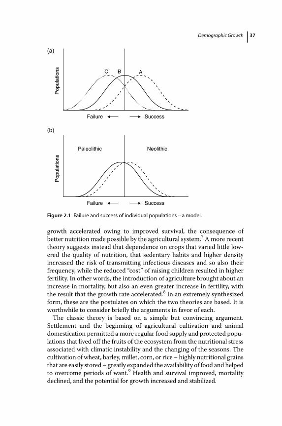
Demographic Growth 37
growth accelerated owing to improved survival, the consequence of better nutrition made possible by the agricultural system.7 A more recent theory suggests instead that dependence on crops that varied little lowered the quality of nutrition, that sedentary habits and higher density increased the risk of transmitting infectious diseases and so also their frequency, while the reduced “cost” of raising children resulted in higher fertility. In other words, the introduction of agriculture brought about an increase in mortality, but also an even greater increase in fertility, with the result that the growth rate accelerated.8 In an extremely synthesized form, these are the postulates on which the two theories are based. It is worthwhile to consider briefly the arguments in favor of each.
The classic theory is based on a simple but convincing argument. Settlement and the beginning of agricultural cultivation and animal domestication permitted a more regular food supply and protected populations that lived off the fruits of the ecosystem from the nutritional stress associated with climatic instability and the changing of the seasons. The cultivation of wheat, barley, millet, corn, or rice – highly nutritional grains that are easily stored – greatly expanded the availability of food and helped to overcome periods of want.9 Health and survival improved, mortality declined, and the potential for growth increased and stabilized.
Failure Success
Failure Success
C
(a)
(b)
B A
NeolithicPaleolithic
Pop
ulat
ions
Pop
ulat
ions
Figure 2.1 Failure and success of individual populations – a model.
A Concise History of World Population38
In recent decades this theory has been questioned and the problem recast in new terms: in sedentary agricultural populations both mortality and fertility increased, but fertility increased more than mortality, and this explains demographic growth.10 Some agree with this hypothesis but believe that the effect on population increase was minimal.11 It is possible, however, that even a slight acceleration of growth made the sedentary groups more stable and less prone to extinction, according to the model shown in Figure 2.1. Yet why should mortality have been higher among farmers than among hunters? Two groups of causes are usually cited in response to this question. The first is based upon the assertion that nutritional levels, from a qualitative (and some claim also quantitative) point of view, worsened with the agricultural transition. The diet of the hunter‐gatherers, which consisted of roots, greens, berries, fruits, and game, was probably more complete than the fare of the sedentary farmers, which, while adequate calorifically, was meager and monotonous because of the heavy dependence upon grains.12 Proof is found in the study of skeletal remains: body size, height, and bone thickness all seem to have declined when hunters settled and became farmers.13 Armelagos and his colleagues come to the conclusion that:
The shift in subsistence pattern had a significant impact on the biological adaptation of prehistoric Nubians. The development of agriculture resulted in a reduction in facial dimensions and concomitant changes in cranial morphology. In addition, the intensification of agriculture led to nutritional deprivation. The pattern of bone growth and development, the occurrence of iron‐deficiency anemia (as evidenced by porotic hyperostosis), microdefects in dentition, and premature osteoporosis in juveniles and young adult females all suggest that later Nubian populations involved in intensive agriculture were experiencing nutritional deficiencies.14
I have cited the preceding passage not because the experience of the Nubians is applicable to all other types of transition (assuming that remains from the various epochs were representative, that there was no immigration, and no errors were made in evaluating the remains), but in order to illustrate the sort of evidence offered in support of the nutritional hypothesis.
The second argument in favor of this theory is of a different and perhaps more convincing nature. The stable settlement of population created the conditions necessary for the onset, spread, and survival of parasites and infectious diseases, which were unknown or rare among mobile and
Demographic Growth 39
low‐density populations.15 Higher demographic concentration acts as a “reservoir” for pathogens, which remain in a latent state awaiting an opportune moment to resurface. The spread of diseases transmitted by physical contact is favored by increased density, and this density in turn increases the contamination of the soil and water, facilitating reinfection. The replacement of the mobile and temporary shelters of nomadic populations with permanent ones encouraged contacts with parasites and other carriers of infectious diseases. In addition, settlement increases the transmissibility of infections brought on by carriers whose life cycle is otherwise interrupted by frequent human movements; this is the case, for example, with fleas, whose larvae grow in nests, beds, or dwellings rather than on the bodies of animals or human beings. With settlement, many animals, domesticated or not, come to occupy a stable place in the human ecological niche, raising the possibility of infection from specifically animal pathogens and increasing the incidence of parasitism. Agricultural technology may also have been responsible for the spread of certain diseases, for example, malaria, which benefited from irrigation and the artificial creation of pools of stagnant water.16 As confirmation of the lower incidence of acute infectious diseases among preagricultural populations, studies of, for example, Australian Aborigines isolated from contact with the white population are cited.17 In general, the small dimensions and mobility of present‐day hunting and gathering groups seem to provide a defense against parasites, just as their relative isolation appears to check the spread of epidemics.18 It should be recalled, however, that many scholars maintain that the biological complexity of the ecosystem (complex in the tropics and simple in desert or arctic areas) is directly related to the variety and incidence of infections affecting populations.19
On the whole, then, a more meager and less varied diet and conditions favorable to infectious diseases would seem to justify the hypothesis of higher mortality among farmers relative to their hunting ancestors.20 But if mortality was higher among farmers, then their more rapid population growth can only have been the result of higher fertility. The latter hypothesis finds support in the social modifications attendant upon the transition from hunting to farming. The high mobility of hunter‐gatherers, continually moving in a vast hunting ground, made the transport of dependent children both burdensome and dangerous for the mother. For this reason, the birth interval must have been fairly long, so that a new birth came only when the previous child was capable of taking care of itself. In a settled society this necessity became less pressing, the “cost” of children in terms of parental investment declined, and their economic contribution in the form of housework, fieldwork, and animal care increased. Paleontological analysis of human skeletons in the necropoleis
A Concise History of World Population40
of Europe, north Africa and north America has revealed systematic changes in the age structure of populations shifting to agriculture that are consistent with an increased fertility.21
The hypothesis that fertility increases with the transition from hunting to agriculture is something more than conjecture. It has, in fact, been confirmed by several studies of present‐day populations. Between 1963 and 1973 a group of scholars led by R. B. Lee studied the !Kung San, a nomadic population that lived by hunting and gathering in northern Botswana (southern Africa) and was at that time beginning a gradual process of settlement.22 Lee’s group observed that about half of the !Kung’s edible vegetables were gathered by the women, who in the course of a year traveled several thousand kilometers. During most of their movements these women carried their children under 4 years of age with them. The age of puberty among the !Kung women was late, between 15 and 17, and a long period of postpuberty sterility followed, so that the first birth came between 18 and 22, followed by birth intervals of 3 to 5 years. These intervals23 are very long for a population not practicing modern birth control and were the result of continuing breast‐feeding until as late as the third or fourth year. Body growth of the babies was slow, a notable adaptive advantage since it allowed their easier transportation during the long daily movements of the mothers. Consequently, the average number of children per woman was fairly low (4.7). Low fertility of this sort, imposed by the habits of hunter‐gatherer populations, is also characteristic of other groups, such as the African Pygmies.24 Still more interesting is the fact that in the process of settlement !Kung San fertility seems to have increased. In fact, the settled women had birth intervals (36 months) significantly shorter than their hunter‐gatherer counterparts (44 months),25 as postulated by the supporters of the theory that fertility increases with the transition from hunting and gathering to farming. The comparison between historical and present‐day populations gives similar results. Two recent studies reveal differences between the total fertility rates (TFR) of hunter‐gatherers (foragers) (5.7 and 5.6) and agriculturalists (6.3 and 6.6).26
The postulates of the two theories are summarized in Figure 2.2. The evidence in their support is for the most part conjectural, and the gathering of data is slow and often contradictory. Both theories assert that the level of nutrition changed, but in opposite ways. Even if it is true that hunter‐gatherers enjoyed a more varied diet (present‐day hunter‐ gatherers seem to be only rarely malnourished), it is hard to imagine that the nutritional level declined with the transition to agriculture. One need only keep in mind the possibility of expanding cultivation, of accumulating reserves, of complementing the products of the earth with those obtained by hunting and fishing, of improving the techniques of food
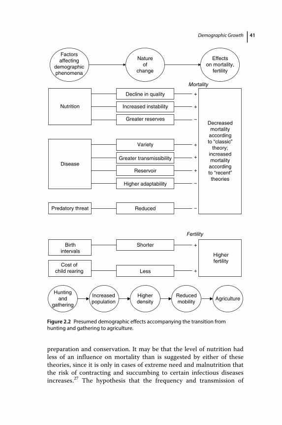
Demographic Growth 41
preparation and conservation. It may be that the level of nutrition had less of an influence on mortality than is suggested by either of these theories, since it is only in cases of extreme need and malnutrition that the risk of contracting and succumbing to certain infectious diseases increases.27 The hypothesis that the frequency and transmission of
Factorsaffecting
demographicphenomena
Natureof
change
+
+
–
+
+
+
+
+
–
–
Increased instability
Greater reservesDecreasedmortalityaccordingto “classic”
theory;increasedmortalityaccordingto “recent”theories
Variety
Greater transmissibility
Reservoir
Higher adaptability
Decline in quality
Nutrition
Disease
Predatory threat Reduced
Birthintervals
Cost ofchild rearing
Shorter
Less
Higherfertility
Huntingand
gathering
Increasedpopulation
Higherdensity
Reducedmobility
Agriculture
Effectson mortality,
fertility
Mortality
Fertility
Figure 2.2 Presumed demographic effects accompanying the transition from hunting and gathering to agriculture.
A Concise History of World Population42
infectious diseases increased in higher‐density and more permanent populations is better founded, though the matter is too complex to allow simplification.28
With regard to fertility, the evidence from present‐day preagricultural groups argues convincingly in favor of the possibility that the transition to settled agriculture entailed increased prolificity. Moreover, Childe, an advocate of the classic theory, noted that in an agricultural society “ children become economically useful; to hunter’s children are liable to be a burden.”29
2.3 Black Death and Demographic Decline in Europe
Around the year 1000 ce the population of Europe began a phase of growth that would last three centuries. The data are scarce and fragmentary, but sufficient to reveal the symptoms of solid demographic growth. Settlements multiplied, new cities were founded, abandoned areas were inhabited, and cultivation expanded to progressively less fertile lands. In the course of these centuries European population increased by a factor of two or three, testimony to a growth potential that frequent crises could not suppress. Toward the end of the thirteenth century and in the first decades of the fourteenth there is clear evidence that this cycle of growth was losing momentum: crises became more frequent, settlements ceased to expand, and here and there population stagnated. This slowdown was the result of complex causes, probably connected to an agricultural economy made less vigorous by the depletion of the best land and a halt in technological progress and subject to more frequent shortages due to unfavorable climatic conditions.30 It might have been a passing phase, a period of adjustment as a population sought a more favorable balance with resources, to be followed by another cycle of growth. Instead, toward the middle of the fourteenth century a devastating and long‐term catastrophe occurred, which caused a population decline, according to the estimates of Table 1.3, by almost a third between 1340 and 1400, only to continue to decline during the first half of the following century before beginning to recover. This recovery would not carry population to its precrisis level until the mid‐sixteenth century.
The catastrophe was the plague; between its first appearance in Sicily, in 1347, and 1352 when it spread through Russia, it traversed the entire continent. Figure 2.3 shows its expansion: by the end of 1348 it had reached Italy, the Iberian Peninsula, part of France, and southern England; by the end of 1349, Norway, the rest of France, the Rhine Valley,
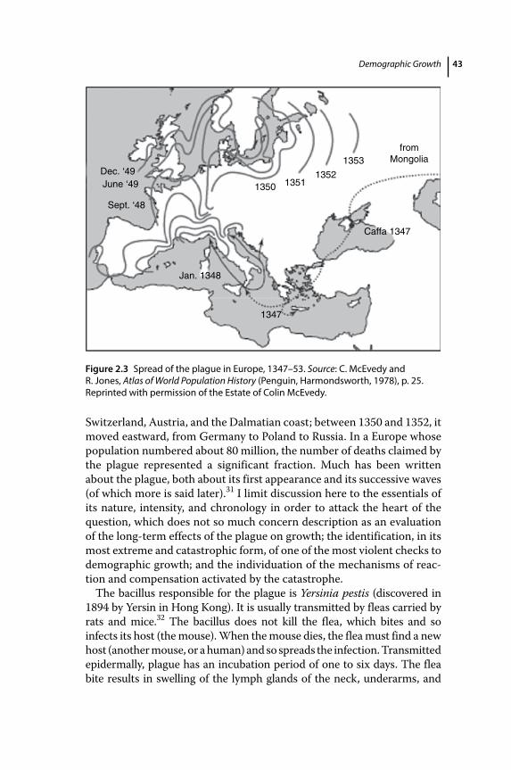
Demographic Growth 43
Switzerland, Austria, and the Dalmatian coast; between 1350 and 1352, it moved eastward, from Germany to Poland to Russia. In a Europe whose population numbered about 80 million, the number of deaths claimed by the plague represented a significant fraction. Much has been written about the plague, both about its first appearance and its successive waves (of which more is said later).31 I limit discussion here to the essentials of its nature, intensity, and chronology in order to attack the heart of the question, which does not so much concern description as an evaluation of the long‐term effects of the plague on growth; the identification, in its most extreme and catastrophic form, of one of the most violent checks to demographic growth; and the individuation of the mechanisms of reaction and compensation activated by the catastrophe.
The bacillus responsible for the plague is Yersinia pestis (discovered in 1894 by Yersin in Hong Kong). It is usually transmitted by fleas carried by rats and mice.32 The bacillus does not kill the flea, which bites and so infects its host (the mouse). When the mouse dies, the flea must find a new host (another mouse, or a human) and so spreads the infection. Transmitted epidermally, plague has an incubation period of one to six days. The flea bite results in swelling of the lymph glands of the neck, underarms, and
1350 13511352
1353from
Mongolia
1347
Jan. 1348
Sept. ‘48
June ‘49Dec. ‘49
Caffa 1347
Figure 2.3 Spread of the plague in Europe, 1347–53. Source: C. McEvedy and R. Jones, Atlas of World Population History (Penguin, Harmondsworth, 1978), p. 25. Reprinted with permission of the Estate of Colin McEvedy.
A Concise History of World Population44
groin (buboes). Symptoms of the disease include high fever, coma, cardiac failure, and inflammation of the internal organs. Normally two‐thirds to four‐fifths of those infected die.33 The plague was easily transmitted, even over long distances, together with goods carrying infected mice or fleas (clothing, personal objects, foodstuffs).
No one is naturally immune to the plague. Those who contract the disease and survive acquire short‐term immunity. Nonetheless, the possibility that successive waves of the plague progressively selected individuals who were for some reason less susceptible to the disease cannot be ruled out, though these processes must evolve over long periods in order to have a perceptible effect.
The plague that appeared in Europe in 1347, while not a new phenomenon, had been absent for six or seven centuries, since the plague of the Justinian period. The latter spread through the eastern Mediterranean in 541–4 and afflicted Italy and Mediterranean Europe in successive waves from 558–61 until 599–600. It remained in the East until the middle of the eighth century, generating successive epidemics, which, though localized, continued to affect Europe.34
In September 1347 the unloading of several Genoese galleys in Messina interrupted long centuries of bacteriological peace. These ships came from ports on the Black Sea where the plague, having arrived from the East, raged. In the space of 4 or 5 years, as mentioned above, the disease traversed the entire continent; and this was only the first of a series of epidemic waves. In Italy (and progress was little different in the rest of Europe) these waves came in 1360–3, 1371–4, 1381–4, 1388–90, and 1398–1400. In the fifteenth century they were still occurring frequently, but with less synchronicity and severity.35 Measurement of the mortality of the various epidemic waves is uncertain due to the lack of precise data. Nonetheless, there were for many areas annual series of deaths from which we can discern the levels of mortality in normal and plague years. In Siena, for example, the plague of 1348 caused 11 times more deaths than normal. In the other five epidemics of that same century the death total increase varied between 5 and 10 times the norm. Imagining that normal mortality was about 35 per 1,000, then an increase of 11‐fold would mean about 420 per 1,000, or the death of more than 4 persons in 10. A 10‐fold increase means, approximately, the elimination of one‐third of the population, an increase of fivefold the elimination of one‐sixth.
For several parts of Tuscany between 1340 and 1400 I have calculated that on average a serious mortality crisis – defined as an increase in deaths at least three times the normal – occurred every 11 years; the average increase in deaths was at least sevenfold. In the period 1400–50 these crises occurred on average every 13 years and deaths increased fivefold. In the following half century (1450–1500) the average frequency
Demographic Growth 45
declined to 37 years and the average increase to fourfold.36 With the passage of time, both the frequency and the intensity of the crises declined, as did the geographic synchronization of their occurrence. Keep in mind that Tuscany is an exceptional case due to the abundance of historical sources to be found there.
The following two centuries were not spared the devastation of the plague, from the cycle of 1522–30 (made worse by the wars that followed the fall of Charles VIII) to that of 1575–77 (especially in the north), 1630–1 (in the center‐north), and 1656–7 (especially in the center‐south).37 Although these bouts of plague were terrible (Cipolla calculates that more than a quarter of the center‐north population struck by the 1630–1 plague was wiped out),38 they were no longer the dominating catastrophes they had been in previous centuries. Other crises (typhus, for example) competed with the plague for the prize. With some variations the Italian experience applies to Europe as a whole. After the epidemic of 1663–70, which hit England (the London plague of 1664 described by Defoe), northern France, the Low Countries, and the Rhine Valley, the plague disappeared from Europe as a general geographic event, except for an appearance in Provence in 1720–2 and in a few other limited areas.39
Returning to our central concern, in the century following the Black Death of 1348 the European population declined both as a result of the first and, from a literary point of view, the most famous plague explosion and also the relentless plague cycles that followed. Only in the sixteenth century would the European population once again attain the numerical level of 1340, while the plague would continue to play a role as a check on population growth until its virtual disappearance in the second half of the seventeenth century. There are no precise data on the scale of the decline between the period before 1348 and the population nadir reached during the first half of the fifteenth century, but a loss of 30 to 40 percent is corroborated by local studies in Piedmont and Tuscany,40 and in France, Spain, England, and Germany. Cities emptied within oversized urban boundaries, abandoned villages, and deserted countryside rendered concrete testimony, while a labor shortage caused salaries to rise and the abundance of available land lowered the price of food.
The plague constitutes a population check largely exogenous, or external, to the sociodemographic system. It acted independently of modes of social organization, levels of development, density of settlement, and so on. The ability of the plague to infect and kill bore no relation to one’s state of health, age, or level of nutrition. It struck urban and rural populations with equal violence and, with the exception of a few isolated areas, density levels presented no obstacle to its spread. The movement of people and goods was sufficient to carry it from one end of the continent
A Concise History of World Population46
to the other. In the long term, of course, societies took measures to defend themselves. The quarantine and isolation of infected or suspect individuals and goods, the shutting up of plague victims’ homes, and a few public health measures may partially explain the disappearance of the plague from the European continent.41 Nonetheless, for over three centuries the plague made itself at home there.
Unlike the victims of many other diseases, the few individuals who contracted the plague and survived did not acquire long‐term immunity. It is not reasonable, then, to attribute the gradual decline of the plague solely to the existence of a larger immunized portion of the population. The process of Durchseuchung, according to which “the accidentally less susceptible survive, and through generations a gradual alteration of the relationship between parasite and host becomes established,”42 may have had some effect; and “had the disease continued, constantly present, and attacking a large portion of the new generations as they appeared, it might gradually have assumed an endemic, sporadic form, with relatively low mortality.”43
A disease of such ferocity could have, after repeated attacks, completely eliminated the populations it infected. This did not happen, and with time the frequency, if not always the intensity, of the crises declined. Neither the specific explanations discussed above (social adjustment, immunity, selection) nor others (either social or ecological transformations) are sufficient to explain this phenomenon. For reasons not entirely clear the plague underwent a process of mutual adaptation between pathogen (Yersinia), carrier (flea), and host‐victim (human).
As occurs for other sorts of mortality crises, there was also a process of sociodemographic adaptation and response to the plague, both in the short and medium to long term. In the short term a sudden and large increase in mortality has a double effect. The spread of the disease lowers the frequency of conceptions, births (for choice, necessity, and psychobiological reasons), and marriages. The decline in births accentuates the negative demographic action of the epidemic. Moreover, high mortality ends marriages and breaks up or destroys family units. At the end of the crisis there is a rebound effect which, while not sufficient to compensate for the lost lives and births, nonetheless attenuates their effect. Marriages that had been postponed during the crisis are celebrated and the marriage rate among the widowed increases. In some cases a fertility increase among couples has even been noted. These several factors combine to produce a temporary increase in overall fertility. Mortality, also, is often below normal after a crisis owing to the reduced representation of infant age groups and the selective effects linked to the epidemic. The balance between births and deaths improves and for a few years some of the previous losses are made up. A new crisis can, of course, soon restart
Demographic Growth 47
the cycle, as in the 100 years after 1348, or it can do so after a longer interval, as in the sixteenth and seventeenth centuries.44
In the long term other factors intervene. Depopulation caused by the plague in Europe created abundant available land and a labor shortage. New family units acquired the resources they needed to establish themselves more easily. The checks to marriage generally relaxed and nuptiality increased, stimulating population growth. One may, for example, explain in this way the low age at marriage in early fifteenth‐century Tuscany.45 Both long‐ and short‐term responses tend to minimize the damage done to society and population by Yersinia, flea, and mouse.
2.4 The Tragedy of the American Indios: Old Microbes and New Populations
“Thrice happy are those, that inhabiting some yet undiscovered island in the midst of the ocean, have never been brought into contaminating contact with the white man.”46 So wrote the young Melville in 1845 on returning from the Marquesas Islands. The tragic effects of contact between white Europeans – whether conquerors, colonists, explorers, or sailors – and the indigenous populations of the New World, the Pacific, and Oceania were evident from the time of the earliest explorations. Historical documentation is abundant, and we have only to choose our examples.
As is well known, Columbus landed in Haiti (christened at the time Hispaniola) in 1492. The number of inhabitants at the time is of course unknown, but it seemed densely populated to the first visitors, “like the countryside of Córdoba.”47 Authors writing a quarter of a century or so later report an original population of 1 million or more, supposedly “counted” by Columbus or his brother Bartolomé in 1495 or 1496 when they tried to impose a gold tribute on the natives. Las Casas – the colonist who became a Dominican friar and staunch defender of the Indios – would eventually increase this number to 3 or 4 million. Modern scholars, since the 1950s, give estimates as widely different as 60,000 and 8 million. Recent estimates, following different strategies (such as the carrying capacity of the island; the production of gold and the possible productivity of native manpower – one‐third of which was sent to the mines; the number of communities and the distribution of villages), seem to point to a contact population of 200,000–300,000 people, subdivided into several hundred communities, each headed by a cacique. In 1514, the Repartimiento – or the allotment of natives to the colonists for personal service, labor in the fields, cattle raising, and gold mining – counted only 26,000 people of both sexes and all ages.48 After the smallpox
A Concise History of World Population48
epidemic of 1518–19 only a few thousand were left and the natives were heading toward extinction. By mid‐century the community had been wiped out; natives still survived as servants of the Spaniards, with a high rate of mixing with the Spaniards themselves, with black slaves carried from Africa, and with other Indios taken from the other islands or the mainland.
What determined the abrupt decline of the Taino population in the three decades following the Conquest and their practical extinction 20 years later? As we shall discuss, one main cause of population decline in the New World was the fact that the native population lacked immunity with respect to many pathologies, unknown in America but common in Eurasia and to which the European settler was well adapted. Diseases relatively harmless in Europe became deadly for the natives: this is called the “virgin soil” effect. The paradigm of a “virgin soil” population and of its vulnerability to new pathologies provides an apparently efficient and convincing answer but, for the Hispaniola case, it has two drawbacks. The first is that there is no historical proof of major epidemics on the island before the smallpox epidemic of 1518–19, when the population was already reduced to 10,000 or less. Contemporary witnesses often made reference to a general situation of very precarious survival, weakness of the population, and continuing high mortality – but not to sweeping and lethal epidemics. The second drawback is that the “virgin soil” paradigm tends to obscure all other factors of population decline, such as the hampering of reproduction owing to deep societal dislocation.
Starting in the second decade of the sixteenth century, when the negative consequences of the decline of the native population for the economy of the island became evident, the debate on the causes of the ongoing demographic catastrophe was rather intense: Las Casas and the Dominicans were active figures in the debate, but so were religious men of other orders; many high administrators and officials; Oviedo, a competent historian who resided in the island. Greed for gold and the encomienda (the practice of allotting the natives to the colonists as indentured labor) are believed to be the principal causes. Greed for gold: too many Indios in the mines and for too long periods (up to 10 months per year); neglect of other productive activities; overwork; lack of food; unsuitable climate and environment in the mines; maltreatment; separation from their families. All these reasons led to high mortality among them and to low fertility of their women. The encomienda system: the Indios were shifted from one part of the island to another; they were frequently moved from one master to another; communal life was disrupted; the encomenderos, fearing the loss of their Indios, exploited and overworked them; concubinage; maltreatment. Under these conditions
Demographic Growth 49
Indios often escaped into the wilderness where, in a hostile environment and away from their normal sources of subsistence, survival was difficult; they committed suicide; they rose in open rebellion; they were victims of violence.
These explanations proposed by competent – although at times biased – eyewitnesses can be summarized as follows: the Spanish conquest caused a deep economic and social dislocation that created the conditions for high mortality and reduced fertility. Economic dislocation was determined by the “procurement,” in favor of the Spanish masters, of native labor subtracted from normal subsistence activities and employed in the production of food, goods, and services for the newcomers and, later, also in the production of gold. Labor employed in the mines had, in its turn, to be supported by native labor working in the fields. This double “attack” on the traditional patterns of production and consumption was deadly for a society based on a subsistence economy and unaccustomed to accumulation. It meant increased work and decreased consumption, and a dramatic worsening of living conditions with an increased vulnerability to scarcity. Although only a few hundred Spaniards were living on the island until the beginning of the sixteenth century, their demands for food, labor, and services were a very heavy burden on the relatively small Taino society.
Social dislocation derived from the encomienda system: Indios were shifted from one place to another and from master to master; their traditional system of life – including communal safety nets – was shattered; some of the women were attracted into the conquerors’ reproductive system (in 1514 there were 83 adult women for every 100 adult men in the native communities); communities, clans, families, couples were divided or separated.
These general causes had a profound impact on the demography of the Taino. Unions were more difficult and precarious; fertility declined. In 1514 children below age 14 made up only 10 percent of the total population, a situation consistent with a rapidly declining population. Living conditions worsened and survival deteriorated, and new diseases (before smallpox), although not responsible for major epidemics, certainly added complexity to the island’s microbial world, increasing current mortality. Together with the economic and social systems, the demographic system of the Taino also collapsed. Cuba, Puerto Rico, Jamaica – less populated than Hispaniola – suffered the same disaster.
Elsewhere on the mainland of America contact with the European intruders had catastrophic consequences, but the natives were not wiped out. Preconquest estimates are based on conjecture and have led experts to suggest widely different population figures, ranging from a minimum of 8 million to a maximum of 113 million for the entire continent; a
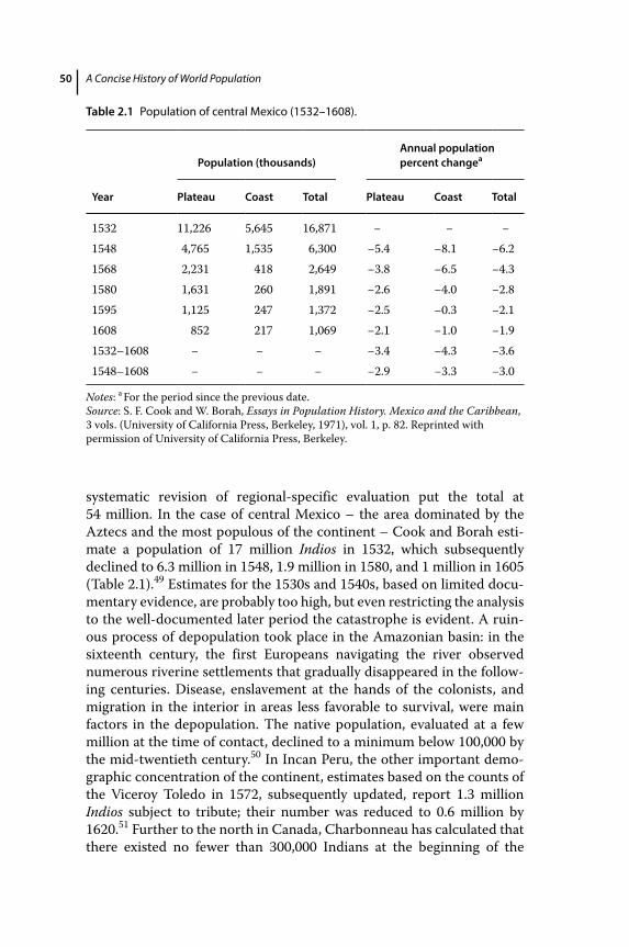
A Concise History of World Population50
systematic revision of regional‐specific evaluation put the total at 54 million. In the case of central Mexico – the area dominated by the Aztecs and the most populous of the continent – Cook and Borah estimate a population of 17 million Indios in 1532, which subsequently declined to 6.3 million in 1548, 1.9 million in 1580, and 1 million in 1605 (Table 2.1).49 Estimates for the 1530s and 1540s, based on limited documentary evidence, are probably too high, but even restricting the analysis to the well‐documented later period the catastrophe is evident. A ruinous process of depopulation took place in the Amazonian basin: in the sixteenth century, the first Europeans navigating the river observed numerous riverine settlements that gradually disappeared in the following centuries. Disease, enslavement at the hands of the colonists, and migration in the interior in areas less favorable to survival, were main factors in the depopulation. The native population, evaluated at a few million at the time of contact, declined to a minimum below 100,000 by the mid‐twentieth century.50 In Incan Peru, the other important demographic concentration of the continent, estimates based on the counts of the Viceroy Toledo in 1572, subsequently updated, report 1.3 million Indios subject to tribute; their number was reduced to 0.6 million by 1620.51 Further to the north in Canada, Charbonneau has calculated that there existed no fewer than 300,000 Indians at the beginning of the
Table 2.1 Population of central Mexico (1532–1608).
Population (thousands)Annual population percent changea
Year Plateau Coast Total Plateau Coast Total
1532 11,226 5,645 16,871 − − −1548 4,765 1,535 6,300 −5.4 −8.1 −6.21568 2,231 418 2,649 −3.8 −6.5 −4.31580 1,631 260 1,891 −2.6 −4.0 −2.81595 1,125 247 1,372 −2.5 −0.3 −2.11608 852 217 1,069 −2.1 −1.0 −1.91532–1608 − − − −3.4 −4.3 −3.61548–1608 − − − −2.9 −3.3 −3.0
Notes: a For the period since the previous date.Source: S. F. Cook and W. Borah, Essays in Population History. Mexico and the Caribbean, 3 vols. (University of California Press, Berkeley, 1971), vol. 1, p. 82. Reprinted with permission of University of California Press, Berkeley.
Demographic Growth 51
seventeenth century; that number was reduced to less than one‐third two centuries later. Thornton claims that in the 300 years after 1500 the Indians of the area that became the United States were reduced from 5 million to 60,000.52 For all of these groups demographic decline from the moment of contact with Europeans seems to have been the rule. There are also more recent examples: Darwin refers to the disappearance of the inhabitants of Tasmania;53 the Maoris experienced rapid demographic decline from the time of the voyages of Captain Cook to the end of the following century;54 and the Australian Aborigines presumably suffered a similar fate. The indigenous population of Tierra del Fuego, 7,000–9,000 in 1871, is now almost extinct.55 In the Amazon basin there are groups which, due to their extreme isolation, have only in the past century come into contact with colonists or explorers and have died off before the eyes of contemporary observers.56
The above examples should suffice. The demographic collapse of indigenous populations as a result of contact with groups of European origin is a widespread and well‐documented phenomenon throughout America and Oceania. The timing, scale, and duration of the decline of course vary according to the historical situation, but one of the basic mechanisms was fairly simple. Indigenous populations were, so to speak, virgin soil for many infectious diseases that they had never before encountered. It would be interesting to study the reverse effect of contact, or the impact of indigenous diseases on European colonists, a subject that has received little attention.57
The initial phase of the Conquest was a deeply brutal affair: people got rich through the mobilization of Indian labor that was employed in the search for gold, the production of subsistence crops, and in personal service of the Spaniards. The reward of the conquistadors was the Repartimento (allotment) of the Indios, which amounted to a forcible confiscation of Indian labor. In Hispaniola, up to one‐third of adult natives were mobilized in the search for gold in the river beds, far from their community of origin (which was often dismembered and assigned to different masters). The same happened in other gold‐yielding areas, in Mesoamerica as in the Andean region. Elsewhere no gold could be found, and the prosperity of the first colonists was based on the abundance of native labor and its mobilization for the construction of urban infrastructure – roads and civil and religious buildings; for the transportation of goods; for the production of food for a growing Spanish population of administrators, clergy, merchants, and craftsmen; for sustaining military expeditions; and for the general functioning of the complex Iberian society that had been transplanted to America. In many areas of the continent Conquest implied war, with its related consequences of destruction, famines, and hunger. For 20 years Peru was devastated by
A Concise History of World Population52
the wars of Conquest and the civil wars among Spanish factions. The armies were small, consisting of a few hundred or, at the most, 1 or 2 thousand soldiers, but supported by native allies several times their number.58 Everywhere, Spanish and Portuguese colonists attracted to their circle native women as concubines or wives that were subtracted from Indian society and from the natives’ reproductive pool. Everywhere, forced migration and social and economic dislocation upset the balance of native society. The European impact went well beyond the transmission of new pathologies that were not the sole factors of population decline. We have seen, earlier in this chapter, that Europe, devastated by half a dozen waves of the deadliest epidemic of all – the plague, much more lethal than the new diseases that struck America – lost perhaps one‐third of its original population, but avoided catastrophe through vigorous recovery after each epidemic episode. However, in native societies, the combination of new diseases and the destructuring of society paralyzed the forces that ensured demographic recovery; reproduction was impaired and the decline in births combined its negative effects with those of high mortality.
Different contexts for the Conquest meant different destinies for native societies. As we observed earlier, the Taino of the Greater Antilles were already on the path to extinction when the first epidemic, smallpox, hit the islands in 1518–19. The brutal impact of the Conquest – together with the uprooting of communities, forced labor, subtraction of native women, and diffused violence – had an impact stronger than that of disease. In the southern hemisphere, in the vast region then called Paraguay – in the basin formed by the Paraná and Uruguay rivers – the Guaraní congregated in the 30 Jesuit Missions underwent a demographic expansion in the seventeenth century and in the first part of the eighteenth century. The fathers protected them against the slave‐seeking expeditions organized by the Brazilians from the São Paulo region, as well as against the exploitation of the Spanish colonists. The fathers encouraged the Guaraní to abandon their seminomadic and promiscuous life, and imposed on them monogamy and marriage at the age of puberty, thus maximizing their fertility. In spite of the recurrent and destructive waves of epidemics (one every 15 years, on average), the Guaraní population recovered after crises and resumed their growth.59 Between these opposite extremes – the Taino and the Guaraní – there was a great variety of situations: in the Andean region of the Inca empire (Ecuador, Peru, Bolivia), the effect of wars and conflicts was prevalent in determining population decline during the first decades after the fall of the Inca empire; in Mexico, on the other hand, where the “pacification” following the Aztecs’ demise was rapid, and the economic and social impact of the Conquest on the natives was not as burdensome as in Peru,
Demographic Growth 53
epidemics had a primary role in determining high mortality. It is possible that the radial conformation of central Mexico, with lines of communication departing from Technochtitlán (later Mexico City) and leading to the four corners of the empire, accelerated the diffusion of the new diseases; on the other hand, the comb‐like configuration of the Inca empire, with its backbone along the Andes and deep valleys running perpendicular to the ocean, had the opposite effect.
Finally, both in Mexico and Peru, the demographic collapse was stronger in the low‐lying coastal areas than in the highlands, owing to both epidemiological and social causes. The impact of new pathologies was accentuated by the hot climate, as happened for malaria in the Gulf of Mexico; conflicts and the concentration of the Spaniards devastated a fragile habitat and determined the expulsion or demise of the native settlers, as happened in Peru. Everywhere, denser and more structured societies had more chances of survival than less complex ones, based on subsistence economies and unable to produce surpluses and invest.60 To sum up, the new microbes explain only part of the catastrophe; other factors must be looked for in the variable process of Conquest and in the social, cultural, and geographical peculiarities of the subjugated native societies.
2.5 Africa, America, and the Slave Trade
Reliable estimates show that between 1500 and 1870 (when the trade was finally abolished) 9.5 million Africans were deported to America as slaves. These were the survivors of a number (a few millions large) of women, men, and children abducted from their villages, many of whom died while being transferred to the coast, or waiting for embarkation on a slave ship, or on board during the long overseas voyage. Of the survivors, about 1.5 million were taken to America before 1700, 5.5 million between 1700 and 1800, and 2.5 million after that date.61 This was a demographic drain that mainly affected West Africa and which combined its effects with those of the slave trade that involved even greater numbers of Africans, northbound and eastbound, along the trading routes of Arab merchants. The consequences of this demographic drain are as yet unstudied, but it is a common opinion that it may have had relevant depressing effects on the population of West Africa. A diverse, almost paradoxical interpretation maintains that this forcible subtraction of conspicuous human resources might have enhanced the living conditions and survival prospects of the populations of origin. However, there is evidence that the populations who paid this enormous contribution to the slave trade were stagnating, if not declining, during
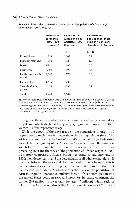
A Concise History of World Population54
the eighteenth century, which was the period when the trade was at its height and which depleted the young age groups – more men than women – of full reproductive age.
While the effects of the slave trade on the populations of origin still require study, much more is known about the demographic regime of the African communities in the New World. We can obtain a synthetic overview of the demography of the African in America through the comparison between the cumulative inflow of slaves in the three centuries preceding 1800 and the stock of the population of African origin in 1800. This stock comprised: Africans brought to America and surviving in 1800; their descendants; and the descendants of all other extinct slaves. If the ratio between the stock and the cumulated inflow is below 1, this is an unequivocal sign that the population is unable to reproduce itself. Let us now consider Table 2.2, which shows the stock of the population of African origin in 1800 and cumulative forced African immigration into the united States between 1500 and 1800: for the entire continent, the former (5.6 million) is lower than the latter (7 million), with a ratio of 0.8:1. In the Caribbean islands the African population was 1.7 million,
Table 2.2 Slaves taken to America (1500–1800) and population of African origin in America (1800) (thousands).
Slaves taken to America (1500–1800)(thousands)
Population of African origin in America, c. 1800(thousands)
Ratio between population of African origin in America and slaves taken to America
(1) (2) (2):(1)United States 348 1,002 2.9Hispanic mainland 750 920 1.2Brazil 2,261 1,988 0.9Caribbean 3,889 1,692 0.4English and Dutch islands
2,060 570 0.3
French islands 1,415 732 0.5Spanish islands (Cuba)
414 390 0.9
Total 7,248 5,602 0.8
Sources: For estimates of the slave trade, Philip Curtin, The Atlantic Slave Trade. A Census (University of Wisconsin Press, Madison), p. 268. For estimates of the population of African origin in 1800, see M. Livi‐Bacci, “500 anos de demografia Brasileira: uma resenha [500 years of Brazilian demographics: a review],” in Revista Brasileira de Estudos de Poblaçaoa 19:1 (2002), pp. 146–7.
Demographic Growth 55
a number less than half the cumulative inflow of 3.9 million slaves (ratio 0.43:1). In Brazil the African population was 2 million, but the total number of slaves received was 2.3 (ratio 0.87:1). The residual 1 million slaves were brought to Hispanic America and to what became the United States, where they found better survival and reproductive conditions.
In Brazil, and even more so in the Caribbean islands, which together absorbed by far the greatest number of slaves, the demographic system of the population of African origin was fueled by the continuous recruitment of slaves, which filled the enormous gaps left by a very high mortality only partially compensated by a weak birth rate. As a consequence the ratio stock/flow was below 1, with a minimum of 0.3 in the English Caribbean. In the United States the ratio was well above 1: reproduction of the slave population was high (TFR of about 8 children per woman) and the mean age at first birth was below 20, the duration of breast‐feeding and birth intervals shorter than in Africa. The slave system did not interfere excessively with marriages and unions, although it posed some de facto obstacles. On the other hand mortality, although higher than among the whites, was much lower than among the slaves in Brazil and in the Caribbean islands. All things considered, the demographic system of the North American population was consistent with a high natural growth.
The causes of the African tragedy in the Caribbean and in Brazil – destinations of six out of seven slave ships – can be found in the living conditions dictated by the loss of freedom, in the way Africans were captured and transported, in the relentless laboring in the sugar plantations, in the adverse conditions under which the adaptation to a new environment, climate, and diets took place. For some Caribbean islands there is firm evidence that fertility was much lower than in the United States, because unions were less frequent, birth intervals longer, the duration of reproductive lifespan lower. There is also evidence of a formidable mortality, particularly high during the period of acclimatization – it was common opinion that between one‐fifth and one‐third of the newly arrived slaves died within 3 years.62 In Brazil it was the common belief at the time that the duration of the active life of a young slave was between 7 and 15 years, and these numbers have acquired the status of incontrovertible truth by force of repetition. The 1872 Census – taken at the end of the slave era, but the data reflect a situation that must have been very similar to that of the past – allows an estimate of life expectancy of slaves of 18 years, against 27 for the entire Brazilian population; these values can be compared with an e0 of 35 for the slave population of the United States at the middle of the nineteenth century.63
If the high mortality of the slave population is out of the question, the debate about its specific determinants is open. There is ample documentation about the heavy labor regime in the sugar plantations
A Concise History of World Population56
(until the end of the eighteenth century this was the main crop) that was under the rigid and merciless control of supervisors. The operations involved required a high input of labor: planting and weeding the fields; cutting, transporting, and crushing the canes; the distillation of molasses; cutting and carrying large quantities of wood for great distances in order to fuel the cauldrons. Operations took place throughout the entire year, and with a production cycle of 9 months that implied the continuous activity of mills and cauldrons, and the work of men and women, from sunrise to sunset and, in the peak periods, through the night.64 Although it was not in the masters’ interests to waste their precious human capital, it has been observed that 2 years of work repaid the capital invested in buying a slave and that in 5 years the initial investment doubled.65 It was inevitable that masters tried to earn the maximum from a minimum of years of the slave’s work. While the diet was adequate, the level of hygiene in the slaves’ compounds (senzala, or large rectangular sleeping quarters where men were separated from women) was appalling, and the care, if not the cure, of the sick and disabled from the part of the masters was certainly poor.
The high mortality rate was not compensated by the low birth rate, depressed by the asymmetrical sex ratio of the slaves taken from Africa (two males for every female). The testimony of the masters, of clergy, of travelers, and of observers is unanimous: they all lament the small number of births. Survival and reproduction were compromised not only by the regime of hard labor – particularly in the sugar plantations in Brazil and the Caribbean – but also by the obstacles to marriages and unions. Giovanni Antonio Andreoni, a Jesuit of Italian origin, renamed “Antonil,” perhaps the most acute and perceptive observer of Brazil in the early‐eighteenth century, wrote that “Many masters are opposed to their slaves’ marriages, and not only they do not object to their illicit unions, but openly consent to them or even start them by saying ‘you, João, in due time will marry Maria’ and from that moment on they let them stay together as if they were husband and wife … others, after that the slaves have married, set them apart in such a way that for long years they remain alone, and this goes against our conscience.”66 The problem was that the masters, although they consented to free unions or even occasional unions, did not encourage (and often discouraged) the marriage of their slaves, jeopardizing the stability and reproduction of the couple, an important factor of the negative balance between births and deaths. In the following century, Saint‐Hilaire observed:
when the campaign in favour of the abolition of the slave trade initiated in Brazil, the Government intimated to the masters of Campos to let their slaves be married; some obeyed the
Demographic Growth 57
intimation, but others answered that there was no point to give a husband to African women that could not raise their children. Soon after giving birth to a child these women were forced to work in the sugar plantations under a scorching sun and when, after being separated from their child for part of the day, they were permitted to be reunited with them, their milk was insufficient: how could the poor creatures survive the cruel miseries of which their masters’ avarice surrounded their cradles?67
Until there was ample supply of slaves on the market, and their price was low, it was more convenient to buy them than sustain the costs of reproduction and child rearing. Other factors came into play, such as the intrusion of the masters in the sexual lives of their women slaves (and the birth of mulattoes who still retained their slave status) and their “subtraction” from the marriage and reproductive pool; or the fact that contacts between slaves of different masters were prohibited or made difficult, thus limiting mating choices. It is thought, also, that the African traditions that were not favorable to monogamy encouraged temporary unions at the expense of the more stable ones.
2.6 The French Canadians: A Demographic Success Story
Having recounted two catastrophic cases of infectious disease‐related mortality – the plague and the virtual extermination of the Indios – let us turn to a demographic success. A few thousand pioneers arrived in the Canadian province of Québec, centered on the St Lawrence basin and five times the size of Italy, in the seventeenth century. Most of the present‐day population of 7.3 million French Canadians (that at the 2011 Census declared French as their mother tongue) trace their ancestry to this original group. Faced with a harsh and inhospitable climate, a few courageous individuals quickly adapted and, thanks to abundant natural resources and available land, rapidly multiplied. In 1776 Adam Smith wrote:
The most decisive mark of the prosperity of any country is the increase of the number of its inhabitants … In the British colonies in North America, it has been found that they double in twenty or five‐and‐twenty years. Nor in the present times is this increase principally owing to the continual importation of new inhabitants, but to the great multiplication of the species. Those who live to old age, it is said, frequently see there from fifty to a hundred, and sometimes many more, descendants from their own body.68
A Concise History of World Population58
Others, from Benjamin Franklin to Thomas Malthus, made similar observations. We shall see that their claims are essentially correct and explain in large part the demographic increase of a few tens of thousands of colonists in North America who, between the eighteenth century and the end of the nineteenth century, became 80 million.
In addition to the vigor of pioneers and colonists, a continual flow of immigration contributed to the demographic success of most of the European populations of North America and Oceania. It has been calculated that in the period 1840 to 1940 a migratory surplus accounted for almost 40 percent of total growth in Argentina, almost 30 percent in the United States, and a little more than 15 percent in Brazil and Canada,69 while in French Canada there was consistently net outmigration.70
The reasons for choosing French Canada as our example are twofold. First, from the eighteenth century onward immigration had little effect on population growth, and second, the Canadian sources are remarkably rich and have been skillfully exploited, allowing analysis of the demographic reasons for the success of the French in America.
Jacques Cartier explored the St Lawrence basin in 1534, and during the following 100 years a French settlement developed there. Québec was founded in 1608; the Company of 100 Associés was formed in 1627 for the purpose of colonization; and in 1663 the royal government took over direction of the colonization process.71 By 1680 the settlement was well established on the banks of the St Lawrence and numbered 10,000 individuals divided among 14 parishes. In the following 100 years the initial nucleus multiplied 11‐fold (from 12,000 in 1684 to 132,000 in 1784, with an average annual growth rate of 2.4 percent), almost entirely owing to natural increase.72
From the foundation of Québec, in 1608, to 1700, total immigration amounted to about 15,000, a tiny fraction of the French population of the day (barely eight emigrants per 1 million inhabitants), while nearby England, with one‐third the population, sent 380,000 emigrants to the New World between 1630 and 1700.73 Careful research has established that barely one‐third of those who immigrated before 1700 (4,997 individuals) successfully established a family in the colony. The others either returned to France, died before marrying, or (in very few cases) remained unmarried. Counting only the true biological “pioneers” who started families before 1680 (a few of these married before immigrating while the majority did so after), we have 3,380 individuals (1,425 women), from whom descend, as already mentioned, the vast majority of French Canadians. Analysis of this group of pioneers and their descendants (see also Chapter 1, Section 1.3) allows examination of the demographic characteristics of the French Canadians and therefore the reasons for their success. These are essentially three: (1) high nuptiality, especially owing to the young age at marriage; (2) high natural fertility; and (3) relatively low mortality.
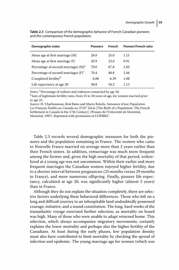
Demographic Growth 59
Table 2.3 records several demographic measures for both the pioneers and the population remaining in France. The women who came to Nouvelle France married on average more than 2 years earlier than their French sisters. In addition, remarriage was much more frequent among the former and, given the high mortality of that period, widowhood at a young age was not uncommon. Within their earlier and more frequent marriages the Canadian women enjoyed higher fertility, due to a shorter interval between pregnancies (25 months versus 29 months in France), and more numerous offspring. Finally, pioneer life expectancy, calculated at age 20, was significantly higher (almost 5 years) than in France.
Although they do not explain the situation completely, there are selective factors underlying these behavioral differences. Those who left on a long and difficult journey to an inhospitable land undoubtedly possessed courage, initiative, and a sound constitution. The long, hard weeks of the transatlantic voyage exercised further selection, as mortality on board was high. Many of those who were unable to adapt returned home. This selection, which always accompanies migratory movements, certainly explains the lower mortality and perhaps also the higher fertility of the Canadians. At least during the early phases, low population density must also have contributed to limit mortality by checking the spread of infection and epidemic. The young marriage age for women (which was
Table 2.3 Comparison of the demographic behavior of French Canadian pioneers and the contemporary French population.
Demographic index Pioneers French Pioneer/French ratio
Mean age at first marriage (M) 28.8 25.0 1.15Mean age at first marriage (F) 20.9 23.0 0.91Percentage of second marriages (M)a 70.0 67.8 1.03Percentage of second marriages (F)a 70.4 48.8 1.44Completed fertilityb 6.88 6.39 1.08Life expectancy at age 20 38.8 34.2 1.13
Notes: a Percentage of widows and widowers remarried by age 50.b Sum of legitimate fertility rates, from 25 to 50 years of age, for women married prior to age 25.Source: H. Charbonneau, Réal Bates and Mario Boleda, Naissance d’une Population. Les Français Établis au Canada au XVII e Siècle [The Birth of a Population: The French Settlement in Canada in the 17th Century]. (Presses de l’Université de Montréal, Montréal, 1987). Reprinted with permission of COPIBEC.
A Concise History of World Population60
initially as low as 15 or 16)74 and the frequency of second marriages owe much to the sexual imbalance created by the greater immigration of males. It was again Adam Smith who observed that:
A young widow with four or five young children, who, among the middling or inferior ranks of people in Europe, would have so little chance for a second husband, is there [in North America] frequently courted as a sort of fortune. The value of children is the greatest of all encouragements to marriage.75
The advantageous conditions in which the pioneers found themselves allowed each couple to have an average of 6.3 children, of whom 4.2 married, with the result that the population doubled in less than 30 years.76 The four‐plus children of the pioneers had in turn 28 children, so that each pioneer had on average 34 offspring between children and grandchildren. About one‐third of the pioneers had more than 50 children and grandchildren, just as Smith wrote in the passage cited earlier.77
Subsequent generations continued to enjoy high levels of reproductivity and rapid growth. While age at marriage for women slowly began to rise as society became more established,78 at the same time the fertility of the daughters of the pioneers, born in Canada and so full participants in the new society, was even higher than that of their mothers (which had in turn been higher than that of the women who remained in France), for example, the average number of offspring for women who married between 15 and 19 years of age in northwest France (the area from which most of the pioneers emigrated) was 9.5; for the pioneers it was 10.1; while for the women born in Canada it was 11.4. For women marrying between 20 and 24, the respective figures were 7.6, 8.1, and 9.5; and for those marrying between 25 and 29 the average numbers of offspring were 5.6, 5.7, and 6.3 respectively.79 The fertility of the Canadians remained high throughout the eighteenth century and is among the highest ever encountered.80 With regard to mortality the situation seems to have been better in the seventeenth than in the eighteenth century, perhaps as a result of increasing density and the declining influence of migrational selection. Nonetheless, Canadian mortality seems to have remained a little better than that of northwest France.81
An initial selection mechanism, social cohesiveness, and favorable environmental factors were the basis of the demographic success of French migration to Canada. A few thousand pioneers at the beginning of the seventeenth century grew in half a century to 50,000,82 initiating the demographic growth shown in Table 2.4. It is interesting to note that while the French Canadian population grew rapidly, that of France (many times larger) grew slowly or stagnated, and the indigenous Indian population, stricken by disease and geographically displaced by colonial
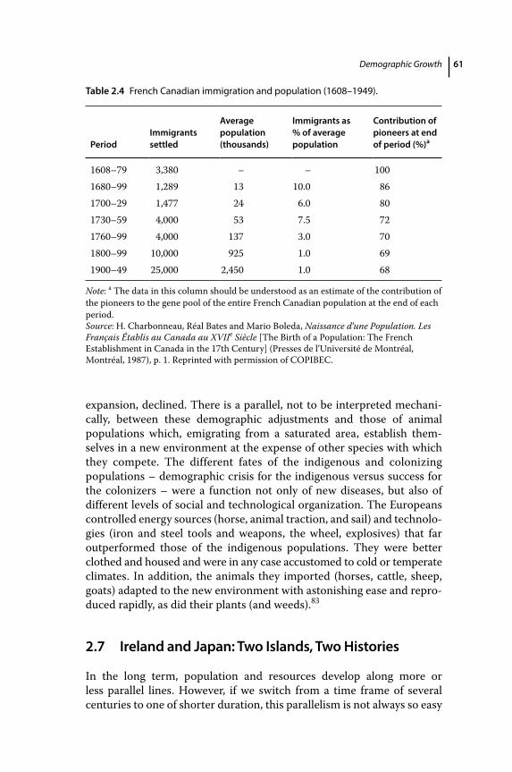
Demographic Growth 61
expansion, declined. There is a parallel, not to be interpreted mechanically, between these demographic adjustments and those of animal populations which, emigrating from a saturated area, establish themselves in a new environment at the expense of other species with which they compete. The different fates of the indigenous and colonizing populations – demographic crisis for the indigenous versus success for the colonizers – were a function not only of new diseases, but also of different levels of social and technological organization. The Europeans controlled energy sources (horse, animal traction, and sail) and technologies (iron and steel tools and weapons, the wheel, explosives) that far outperformed those of the indigenous populations. They were better clothed and housed and were in any case accustomed to cold or temperate climates. In addition, the animals they imported (horses, cattle, sheep, goats) adapted to the new environment with astonishing ease and reproduced rapidly, as did their plants (and weeds).83
2.7 Ireland and Japan: Two Islands, Two Histories
In the long term, population and resources develop along more or less parallel lines. However, if we switch from a time frame of several centuries to one of shorter duration, this parallelism is not always so easy
Table 2.4 French Canadian immigration and population (1608–1949).
PeriodImmigrants settled
Average population (thousands)
Immigrants as % of average population
Contribution of pioneers at end of period (%)a
1608–79 3,380 – – 1001680–99 1,289 13 10.0 861700–29 1,477 24 6.0 801730–59 4,000 53 7.5 721760–99 4,000 137 3.0 701800–99 10,000 925 1.0 691900–49 25,000 2,450 1.0 68
Note: a The data in this column should be understood as an estimate of the contribution of the pioneers to the gene pool of the entire French Canadian population at the end of each period.Source: H. Charbonneau, Réal Bates and Mario Boleda, Naissance d’une Population. Les Français Établis au Canada au XVIIe Siècle [The Birth of a Population: The French Establishment in Canada in the 17th Century] (Presses de l’Université de Montréal, Montréal, 1987), p. 1. Reprinted with permission of COPIBEC.
A Concise History of World Population62
to identify. This situation comes about because the human species is extremely adaptable and able both to withstand periods of want and also to accumulate large quantities of resources. Nor is it the case that demographic variation always reflects, in a period short enough to render causality obvious, the variations in available resources (which we shall consider here, for the sake of convenience, as independent of human intervention). Furthermore, some of the factors influencing demographic change, above all mortality (see Sections 2.3 and 2.4), are independent of resource availability. In some cases, however, the interrelationship between resources and demography is clearly evident. If we accept the authoritative interpretations offered, the examples of Ireland and Japan – two islands distant from one another both in culture and space – between the seventeenth and nineteenth centuries represent this relationship well.
Ireland has always been one of the poorest countries of western Europe. Its population, subjugated by the English, deprived of independence and autonomy, and subject to an agricultural tributary economy dominated by absentee landlords, suffered a backward existence. In spite of poverty it grew rapidly, even more rapidly than nearby England, which was by far the most demographically dynamic of the large countries of Europe. Between the end of the seventeenth century and the census of 1841 – a few years before the Great Famine that would alter Irish demography dramatically – the Irish population grew from just over 2 million to over 8 million (Table 2.5). Japan, although closing itself off to foreign influence, experienced a significant internal revival from the beginning of the Tokugawa era in the early seventeenth century. Population tripled in 120 years and then entered a long period of stagnation until the second third of the nineteenth century. What were the reasons for rapid growth in both cases, and then catastrophe in Ireland and stagnation in Japan?
The case of Ireland was considered by Connell84 over 60 years ago, and his analysis has withstood the scrutiny of subsequent studies reasonably well. Connell’s thesis basically is that a natural tendency of the Irish to marry early was inhibited by the difficulty of obtaining land on which to build a house and start a family. This obstacle was removed in the second half of the eighteenth century by a series of complex factors – among them the great success of the potato – that allowed the extension and breaking up of farmland. As a result nuptiality increased and, together with a high level of natural fertility and a not too high level of mortality, this resulted in a high rate of growth. Finally, this equilibrium became precarious as a result of excessive growth until the Great Famine of 1846–7 permanently upset the previous demographic order.
The data in Table 2.5 show rapid Irish demographic growth: in the century prior to 1845 the population grew at an annual rate of 1.3 percent
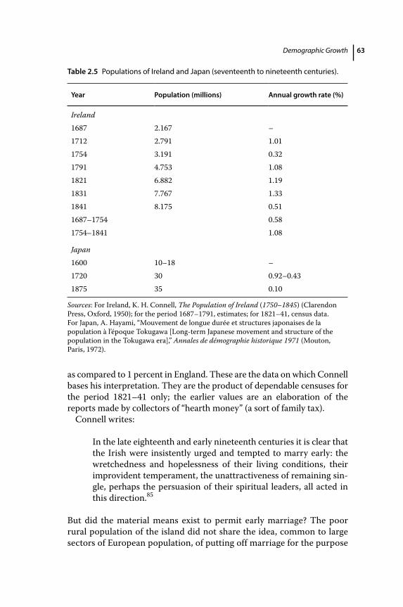
Demographic Growth 63
as compared to 1 percent in England. These are the data on which Connell bases his interpretation. They are the product of dependable censuses for the period 1821–41 only; the earlier values are an elaboration of the reports made by collectors of “hearth money” (a sort of family tax).
Connell writes:
In the late eighteenth and early nineteenth centuries it is clear that the Irish were insistently urged and tempted to marry early: the wretchedness and hopelessness of their living conditions, their improvident temperament, the unattractiveness of remaining single, perhaps the persuasion of their spiritual leaders, all acted in this direction.85
But did the material means exist to permit early marriage? The poor rural population of the island did not share the idea, common to large sectors of European population, of putting off marriage for the purpose
Table 2.5 Populations of Ireland and Japan (seventeenth to nineteenth centuries).
Year Population (millions) Annual growth rate (%)
Ireland1687 2.167 –1712 2.791 1.011754 3.191 0.321791 4.753 1.081821 6.882 1.191831 7.767 1.331841 8.175 0.511687–1754 0.581754–1841 1.08
Japan1600 10–18 –1720 30 0.92–0.431875 35 0.10
Sources: For Ireland, K. H. Connell, The Population of Ireland (1750–1845) (Clarendon Press, Oxford, 1950); for the period 1687–1791, estimates; for 1821–41, census data. For Japan, A. Hayami, “Mouvement de longue durée et structures japonaises de la population à l’époque Tokugawa [Long‐term Japanese movement and structure of the population in the Tokugawa era],” Annales de démographie historique 1971 (Mouton, Paris, 1972).
A Concise History of World Population64
of accumulating capital and attaining a better standard of living.86 The large landowners tended to limit their tenants to a subsistence existence by adjusting rents, and so rendered difficult any improvement in the standard of living. The cost of marriage was small; a new dwelling, usually little more than a shack, could be constructed in a few days with the help of friends and family; and furniture was simple and rudimentary.87 The real problem in a society of tenant farmers was the availability of a plot on which to establish a new household. As long as this was difficult (for example, dependent on the death of the father), nuptiality was checked. However, toward the end of the eighteenth century conditions changed. The conversion of pasture to cultivated plots and the cultivation of new lands (reclaimed swamps and mountains) – promoted by reforms of the Irish Parliament and by the demand in England, which was at war with France, for foodstuffs – removed this check.88 Land subdivision increased still more as a result of the introduction and spread of the potato, which quickly became the primary, and often almost sole, food of the Irish.89 The special role of the potato, perhaps introduced by Sir Walter Raleigh at the end of the sixteenth century and then gradually adopted, was decisive for two reasons. The first was its high productivity. As the population became ever more dependent upon the potato, “land which formerly had been adequate for only one family’s subsistence could be parceled among sons or other subtenants,”90 since “an acre of potatoes sufficed to feed a family of six and the livestock.”91 The second reason was the high nutritional value of the potato, consumed in incredible proportions as part of a diet which also included a considerable amount of milk.92 Arthur Young, traveling in King’s County, observed: “their food is potatoes and milk for ten months and potatoes and salt for the remaining two.”93 A barrel of 280 lbs (127 kg) of potatoes fed a family of five for a week at an average daily consumption of 8 lbs (3.6 kg) per person, including infants and children. Connell estimates daily consumption at 10 lbs between 1780 and the Great Famine, while Salaman suggests 12 lbs per adult at the end of the eighteenth century, “a quantity exceeded in the next century.”94 It should be added that a diet of 4 kg of potatoes and half a liter of milk contains more than sufficient caloric and nutritional value for an adult male.95 So while one may accuse the potato of having impoverished the Irish peasantry, one cannot accuse it of having exposed them to higher mortality. The availability of new land and the fragmentation of existing plots, made more productive due to potato cultivation, enabled the low age at marriage and high nuptiality of the Irish. These factors, combined with high natural fertility96 and moderate mortality, produced a high rate of growth in the period leading up to the Great Famine.97
Demographic Growth 65
Sustained demographic growth (the population doubled between 1781 and 1841) in a rural society for which land, even though made more productive by the introduction of the potato, was the limiting factor of production could not go on indefinitely. Already in the decade before 1841 there is evidence of a gradual rise in the age at marriage and increased emigration. These developments did not, however, avert catastrophe: in 1845 a fungus, Phytophthora infestans, badly damaged the potato harvest; in 1846 it destroyed it entirely.98 The winter of 1846–7 brought famine, poverty, desperate and massive emigration, and epidemics of fevers and typhus. It has been estimated that the Great Famine, together with associated epidemics, caused between 1.1 and 1.5 million more deaths than normal.99 Emigration became an exodus, and 200,000 people per year left Ireland between 1847 and 1854.100
The Great Famine marked the end of a demographic regime. The potato contributed to rapid demographic growth, but also rendered precarious the diet of a population that depended upon it alone for its nutritional needs. During the following decades a new regime of land use and ownership and a new nuptial order (late marriage and high rates of spinsterhood and bachelorhood), supported by the large landowners and the clergy, together with massive emigration resulted in a steady decline in population. The average age at first marriage increased from 23–24 between 1831 and 1841, a level already above that of previous decades, to 27–28 at the end of the century. The proportion of married women of childbearing age declined sharply between 1841 and the end of the century,101 when about one‐fifth of the population aged 50 had never married. The island’s population declined rapidly from 8.2 million in 1841 to 4.5 million in 1901.
According to the interpretation of one of the most authoritative scholars of Japanese demographic and social history,102 the case of Japan resembles that of Ireland in the initial phase, though of course the setting is very different. The Tokugawa regime, which stretched over more than two‐and‐a‐half centuries from 1603 to 1867 and the beginning of Meiji‐era modernization, was characterized by domestic peace, closure to both the outside world and Christian penetration, a revival of Confucianism, and political stability. However, during this long period:
society prepared itself for modernization, … economically motivated behavior gradually modified the lifestyle of the population … Initially production, which served to pay off property taxes and meet individual needs, had poverty as its inevitable accompaniment, … but when the principal end of production became selling, then suffering became the work by means of which one was able to prosper and improve the qualities of one’s life.103
A Concise History of World Population66
The amount of cultivated land doubled and agricultural techniques changed from extensive to intensive. Traditional social structures altered: large family groups, including many relatives and servants who were generally not able to marry, were broken up and many independent families established. In the county of Suwa, for example, average family size declined from 7 in the period 1671–1700 to 4.9 in 1751–1800.104 The servant class of the Genin,105 only a small fraction of which ever married, was transformed into a class of tenant farmers characterized by normal demographic behavior.
The freeing up of economic resources (new lands, new agricultural technology) was accompanied by sustained demographic growth. Hayami estimates a population of no more than 10 million at the beginning of the seventeenth century, which grew rapidly to 30 million by 1720 (the uncertainty of the sources induces him to adopt a safety margin of plus or minus 5 million), maintaining an average annual rate of growth of between 0.8 and 1 percent for over a century.106 In the following century and a half this galloping growth slowed to a trot: in 1870, just after the fall of the Tokugawa regime, the population was about 35 million, having grown since 1720 at the reduced annual rate of 0.2 percent. The causes and mechanisms of this stagnation are the subject of considerable debate. There is definite evidence of intentional control of the “production” of children, not so much by delaying marriage but by the practices of abortion and infanticide, and of a “destructive” role played by the cities with regard to the rural population surplus (Edo, today Tokyo, was the largest city in the world at the beginning of the nineteenth century). Detailed studies of several Tokugawa‐era villages supply ample documentation, as a complement to literary and legal reports, attesting to the widespread practice of abortion and infanticide in all social classes.107 In the village of Yokouchi, for example, women born before 1700 and married at 20 years of age bore on average 5.5 children, while those married at the same age but born between 1750 and 1800 averaged barely 3.2.108 Beyond infanticide and abortion, another interesting explanation for the slow population growth of the late Tokugawa epoch and the Meiji epoch that followed is the well‐documented agricultural transformation that took place and led to an ever greater intensification of farming methods. This transformation improved the general conditions of rural life but also brought with it a notable increase in workloads for men and even more for women. This trend “must have had unfavourable effects on marital fertility, as well as on infant and maternal mortality, and thereby must have counterbalanced some of the favourable demographic effects of long‐term agrarian development.”109 Whatever the explanation of the demographic stagnation, Japanese society gradually discovered mechanisms to limit demographic growth as the expansion of cultivation encountered natural and insuperable limits.
Demographic Growth 67
The Japanese demographic system differed from the Irish in its response to the gradual pressure applied to available resources. In Ireland the system collapsed with the Great Famine and the Great Emigration: this double shock opened the way to changes in the nuptial regime (high ages at marriage and large numbers of unmarried people). In Japan the response was gradual and not the result of traumatic events.
2.8 On the Threshold of the Contemporary World: China and Europe
With the eighteenth century a large part of the world seemed to enter a phase of demographic acceleration. The word “seems” is appropriate because, if we exclude Europe and America, quantitative information is scant almost everywhere; however, if we give credit to the estimates in Table 1.3, the world population increased 40 percent between 1700 and 1800; a similar increase had been achieved in the two centuries leading up to 1700. While in Africa it is believed that the population was stagnating, estimates indicate a doubling of the population in America, and substantive increases in Europe (54 percent) and Asia (46 percent). What determined this acceleration? How, and for what reasons, did the demographic system undergo a change?
I will examine here the parallel cases of Europe and China. There is some agreement in the literature that, during the eighteenth century, there was considerable population growth in China – numbers more than doubled from about 160 million in 1700 to about 330 million in 1800 – but that this dynamism lost some of its momentum in the following century, particularly after 1850. The growth in the eighteenth century is attributed by many to a favorable phase of economic expansion reflected in the increase in land values and of agricultural production and encouraged by a reduction of the fiscal pressure on the population.110
As a consequence there was a general increase in the standard of living that stimulated demographic expansion. Admittedly, a rather generic explanation, that implies that demographic behaviors are solely shaped by material living conditions. A few contemporary authors have underlined the plasticity of the Chinese demographic system’s ability to adapt to external constraints through a variety of mechanisms.111 First, infanticide permitted the regulation, at family level, of the number and gender composition of offspring. In the majority of cases this was infanticide of baby girls; the incidence was high, reaching 10 percent for the children of women belonging to the imperial lineage, but much higher among children of women of inferior rank. In a sample of peasants born between 1774 and 1873 it has been estimated that between one‐fifth and
A Concise History of World Population68
one‐quarter of baby girls fell victim to infanticide.112 The interpretation is that infanticide was a response to the fluctuations in living conditions.
Selective infanticide, and the higher mortality of surviving baby girls owing to child neglect, generated distortions of the marriage market for the scarcity of eligible women; their scarcity was made worse by a common polygyny and by the low frequency of remarriage among young widows. The result was that almost all women married very young, while men married substantially later and a high proportion remained unmarried. The proportion of women between age 15 and age 50 who were married was much higher than in Europe (typically 90 percent against 60 percent or less). This system of almost universal marriage for women was itself articulated in a variety of institutional forms adaptable to different circumstances: beside the largely dominant patrilocal form (the new couple coresided with the husband’s family), there were alternative forms of uxorilocal type, forms of levirate (for the very poor), polygyny (for the wealthy), and adoptions of baby girls who became spouses of a member of the adoptive family.
The high proportion of married women was balanced by the level of fertility within marriage, which was lower than in Europe. The total number of children born to women married at age 20 (and remaining married until age 50) was around 6, against 7.5 or more for European women.113 Birth intervals were longer than for European women and the age at birth of the last child lower. Peripheral to the low marital fertility may have been a philosophical and religious tradition prescribing sexual continence. Finally, adoption was relevant in the Chinese family system and significant proportion of children – up to 10 percent – were raised by an adoptive family. Adoptions were extended to adolescents and even adults:
Thus the Chinese demographic system was characterized by a multiplicity of choices that balanced romance with arranged marriage, marital passion with marital restraint, and parental love with the decision to kill or give away children, and the adoption of other children … Chinese individuals constantly adjusted their demographic behavior according to collective circumstances to maximise collective utility.114
During the first part of the nineteenth century, the Chinese population continued its fast growth (from 330 to 430 million) but at a lower rate, while rebellions and bloody conflicts (the Taiping War between 1851 and 1864 was particularly destructive) and the hardship of famines caused a violent setback in the third quarter of the century and a slow successive recovery. During the nineteenth century, owing to the limitation of land,
Demographic Growth 69
of decreasing returns from agriculture, of lack of innovation and delay in the adoption of the fruits of the technological revolution, the impoverished population adopted preventive and repressive checks to demographic growth.115 For some authors, the plasticity of the Chinese demographic system – based also on the destructive practice of infanticide – played the roles of “accelerator” of growth in the eighteenth century and of “brake” in the nineteenth. This interpretation is not shared by others, for whom the second part of the nineteenth century was dominated by the destructive impact of subsistence crises and ensuing high mortality, and who assign a minor role to the endogenous, self‐ regulatory action of the population. China, at the end of the nineteenth century, appears to be far from modernity, even in its demographic profile.
The demographic acceleration of Europe in the eighteenth century, reinforced in the nineteenth, was caused by factors different from those of contemporary China. In the early phase the forces of constraint were still strong. Birth control was still virtually unknown except in a few isolated cases, like France, and medical and sanitary measures had made little headway against high mortality. Then, between 1750 and 1850, European population growth accelerated. The annual rate of growth, barely 0.15 percent between 1600 and 1750, grew to 0.63 percent between 1750 and 1850 (see Table 1.3). This acceleration involved all the major countries (see Table 2.6), though it was greater in some (for example, England) than in others (France). However, in spite of the disappearance of the plague and the success in combating smallpox (Jenner discovered a vaccine in 1797) the period between the mid‐eighteenth and mid‐nineteenth centuries was not free of trouble. The French Revolution and Napoleonic wars devastated Europe for 20 years; the last great subsistence crisis – the 1816–17 famine accompanied by an outbreak of typhus – hit all of Europe;116 and a previously unknown pestilence, cholera, ravaged the continent. Nonetheless, the population grew vigorously and spilled over, with the beginning of large‐scale transoceanic migration to the Americas.
A debate – which is still open – has developed regarding the causes of demographic acceleration from the mid‐eighteenth century, in part because the demographic mechanisms themselves are not entirely understood. In some cases growth was due to increased fertility resulting from increased nuptiality, while in the majority, mortality decline was the principal factor.
In the case of England, the country that experienced the greatest demographic growth in the period, recent studies117 ascribe the demographic acceleration of the second half of the eighteenth century to fertility increase (aided by nuptiality increase) rather than to mortality decrease. Apparently the Industrial Revolution generated a notable
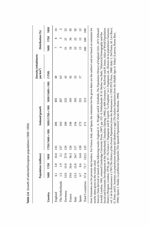
Tabl
e 2.
6 G
row
th o
f sel
ecte
d Eu
rope
an p
opul
atio
ns (1
600–
1850
).
Popu
latio
n (m
illio
ns)
Inde
xed
grow
thD
ensi
ty (i
nhab
itant
s pe
r km
2 )D
istr
ibut
ion
(%)
Coun
try
1600
1750
1850
1750
(160
0 =
100)
1850
(175
0 =
100)
1850
(160
0 =
100)
(175
0)16
0017
5018
50
Engl
and
4.1
5.8
16.6
141
286
405
487
814
The
Net
herla
nds
1.5
1.9
3.1
127
163
207
633
32
Ger
man
y12
.015
.027
.012
518
022
542
2121
22Fr
ance
19.6
24.6
36.3
126
148
185
4534
3430
Italy
13.5
15.8
24.7
117
156
183
5223
2220
Spai
n6.
78.
614
.812
817
222
117
1212
12To
tal 5
cou
ntrie
s57
.471
.712
2.5
125
171
213
100
100
100
Not
e: Es
timat
es a
re fo
r pre
sent
‐day
bor
ders
. For
Fra
nce,
Ital
y, an
d Sp
ain,
the
estim
ates
for t
he g
iven
dat
es a
re th
e au
thor
’s an
d ar
e ba
sed
on e
stim
ates
for
near
by d
ates
giv
en in
the
wor
ks c
ited.
Sour
ces:
Dat
a de
rived
or b
ased
on
the
follo
win
g w
orks
: Eng
land
: E. A
. Wrig
ley
and
R. S
chof
ield
, The
Pop
ulat
ion
Hist
ory
of E
ngla
nd 1
541–
1871
(Edw
ard
Arn
old,
Lon
don,
198
1, re
issu
ed C
ambr
idge
Uni
vers
ity P
ress
, 198
7), p
p. 5
32–4
; Net
herla
nds:
B. H
. Slic
her v
an B
ath,
“His
toric
al D
emog
raph
y an
d th
e So
cial
and
Eco
nom
ic D
evel
opm
ent o
f the
Net
herla
nds,”
Dae
dalu
s (Sp
ring,
196
8), p
. 609
; Ger
man
y: C
. McE
vedy
and
R. J
ones
, Atla
s of W
orld
Pop
ulat
ion
Hist
ory
(Pen
guin
, Lon
don,
197
8), p
p. 6
7–70
; Fra
nce:
J. D
upâq
uier
and
B. L
epet
it, “L
a Pu
epla
de,”
in J.
Dup
âqui
er, e
d., H
istoi
re d
e la
popu
latio
n Fr
ança
ise,
vo
l. 2:
de l
a Re
naiss
ance
à 1
789
[The
His
tory
of t
he F
renc
h Po
pula
tion
from
the R
enai
ssan
ce to
178
9] (P
UF,
Par
is, 1
988)
: Ita
ly: L
. Del
Pan
ta, M
. Liv
i‐Bac
ci,
G. P
into
, and
E. S
onni
no, L
a po
pola
zion
e Ita
liana
dal
Med
ioev
o a
oggi
[The
Ital
ian
Popu
latio
n fr
om th
e Mid
dle A
ges t
o To
day]
(Lat
erza
, Rom
a‐Ba
ri,
1996
); Sp
ain:
J. N
adal
, La
pobl
ació
n Es
paño
la [T
he S
pani
sh P
opul
atio
n] (A
riel,
Barc
elon
a, 1
984)
.
Demographic Growth 71
increase in the demand for labor, which in turn stimulated nuptiality and so fertility (the latter was not yet subject to “control” within marriage). However, mortality also declined, and the combined effect resulted in sustained demographic growth and the tripling of the population in a century. I shall return to England when analyzing the relationship between demographic and economic systems in Chapter 3.
In much of Europe the transition from the eighteenth to the nineteenth century brought with it a decline in mortality. This improvement is evident above all in the lower frequency of mortality crises resulting from epidemic outbreaks and, at times, famine and want. As an example, in a group of 404 English parishes the frequency of months marked by severe mortality was 1.3 percent in the first half of the eighteenth century, 0.9 percent in the second half, and 0.6 in the first quarter of the nineteenth century,118 a sign of the rapid decline of crisis frequency. In France the incidence of severe crises declined dramatically between the first and second halves of the eighteenth century, so much so that one speaks of the end of ancien régime crises, like that, for example, after the harsh winter of 1709, which resulted in a million deaths more than normal or the equally severe crises of 1693–4 and 1739–41.119 In other parts of Europe – Germany, Italy, Spain – the decline occurs later and less suddenly.
The causes for the attenuation of the great mortality crises are at once biological, economic, and social. The biological effect of mutual adaptation between pathogen and host (see Sections 2.3 and 2.4), furthered by increased population density and mobility, cannot be ruled out as a cause for the reduced virulence of certain diseases. Social causes, instead, include the reduced transmissibility of infection as a result of improved private and public hygiene. Finally, economic causes pertain not only to agricultural progress, but also to the improved system of transportation, and so of the distribution of goods, between areas of abundance and areas of want.
The disappearance of crisis years alone, however, does not explain European mortality decline. Life expectancy at birth, for example, increased in England from 33 to 40 years between 1740–9 and 1840–9, in France the same period witnessed an increase from 25 to 40, in Sweden from 37 to 45 (between 1750–9 and 1840–9), and in Denmark from 35 to 44 (between 1780–9 and 1840–9).120 Clearly mortality decline, whether “crisis” or “normal,” was responsible for accelerated demographic growth. One of the theories that has gained favor in recent years is the “ nutritional” theory championed by McKeown,121 according to which eighteenth‐ century demographic acceleration was due to mortality decline; mortality decline, however, cannot be explained by
A Concise History of World Population72
medical advances (ineffective, except for the smallpox vaccine, until the end of the nineteenth century), or by changes in public or private hygiene (which in some cases, for example, the large cities, probably deteriorated), or by other causes. The true cause, according to McKeown, was the improvement of the population’s nutritional level, which increased organic “resistance” to infection. This improvement came about as a result of the progress made in agricultural productivity thanks to the introduction of new, more abundant, crops, from corn to potatoes.
This theory is countered by a number of considerations that make us look to other causes. In the first place, the link between nutrition and resistance to infection holds primarily in cases of severe malnutrition; and while these were frequent during periods of want, in normal years the diet of European populations seems to have been adequate.122 Second, the latter half of the eighteenth century and the first decades of the nineteenth, the period during which this mortality “transition” began, do not appear to have been such a fortunate epoch. It is true that new crops spread. By the second half of the eighteenth century the potato, its diffusion furthered by the severe famine of 1770–2 in the center‐north, had overcome its strongest European doubters and would soon be widespread. A field planted with potatoes could feed twice or thrice the population of a similar field of grain. Versatile buckwheat could be planted late in the season, should the winter crop fail. Corn spread in Spain in the seventeenth century and then passed to southwest France, the Po Valley in northern Italy, and on to the Balkans. As with the potato, its cultivation spread as a result of the subsistence crisis of 1816–17.123 In many cases, however, the introduction of new crops did not improve per capita consumption. Often, as in Ireland with the potato, the new crops served to feed the additional population but led to the abandonment of more esteemed foods, like grains, and so made for a poorer diet. Cobbett’s invective regarding his travels in Ireland is famous in this regard: “It is both my pleasure and my duty to discourage in any way I can the cultivation of this damned root, being convinced that it has done more harm to mankind than the sword and the pestilence united.”124 In England and also in Flanders, there are indications that as potato consumption increased, that of grains declined. In those regions where corn met with greatest success, especially Italy, it became the principal foodstuff and was responsible for the terrible spread of pellagra.125
Other, indirect, considerations also cast doubt on the nutritional hypothesis. For one, real wages in general declined throughout Europe during the eighteenth century and into the first decades of the nineteenth.126 Real‐wage decline is an indication of diminished buying power on the part of salaried workers (and perhaps other groups as well), who in this period spent about four‐fifths of their wages on food. Another
Demographic Growth 73
indication is variation in average height, which seems in this same period to have declined in England, in the Hapsburg Empire, and in Sweden. Height is fairly sensitive to changes in nutritional levels, and its decline or stagnation is certainly not a sign of nutritional improvement.127 Finally, mortality improvement benefited primarily the young (as is always the case when it is due to a decline in infectious disease mortality, a relatively less important cause of death at older ages) and infants. Until weaning, which occurred fairly late, generally between the ages of 1 and 2, babies were fed mother’s milk and so their nutritional level was generally independent of agricultural production and levels of consumption. But infant mortality declined as well, not because of better nutrition, but because of improved child‐rearing methods and better protection from the surrounding environment.
Mortality decline was certainly due to many causes (see Section 4.2) and perhaps none, taken singly, predominated. However, even given a generous reading, the nutritional hypothesis stands up less well to scrutiny than others. It is nonetheless the case that increased agricultural production accompanied European demographic expansion (the population almost doubled in a century), even if nutritional levels did not improve notably. While the possibility of farming new lands – once pasture, swamp, or wild – together with improved technology and the introduction of new crops may not have been responsible for mortality decline, these elements did allow the agricultural population to expand, forming new centers and increasing nuptiality levels. The growth of the industrial sector, urbanization, and a general increase in demand for nonagricultural labor assisted this process and created an outlet for the rural population.
Notes
1 V. G. Childe, Man Makes Himself (Mentor, New York, 1951), p. 51. L. Cavalli Sforza and F. Cavalli Sforza, “Moderni da Centomila Anni,” Il Sole 24 Ore (July 9, 2000).
2 J. R. Harlan, “Agricultural Origins: Centers and Noncenters,” Science 174 (1971).3 An indirect proof of demographic growth contemporary with the
domestication of plants and animals in the Near East, about 8000 bce, is given by the successive waves of migration to the northeast; and these in turn were likely to be the primary cause of the expansion of agricultural technology. “One consequence of the introduction of agriculture, of course, is an increase in the number of people who can live in a given area. Such an increase in population is often accompanied by a wave of expansion: early farming was in itself a shifting type of agriculture that required frequent movement from old fields to new ones.” The average
A Concise History of World Population74
annual amount of expansion was about 1 km. This is the theory developed by Cavalli Sforza and Ammerman, who have identified the beginning of agriculture in the various zones of Europe by carbon‐14 dating the oldest remains of cultivated plants. See L. L. Cavalli Sforza, “The Genetics of Human Population,” Scientific American (September 1974), pp. 80–9, from which the above quotation is taken. See also A. J. Ammerman and L. L. Cavalli Sforza, “A Population Model for the Diffusion of Early Farming in Europe,” in C. Renfrew, ed., The Explanation of Culture Change (Duckworth, London, 1973).
4 J. N. Biraben, “Essai sur l’Évolution du Nombre des Hommes [Essay on the Evolution of the Population],” Population 34 (1979). See also Table 1.1 in this volume.
5 The significance of comparisons between growth rates of this sort, based on uncertain data and referring to long periods and vast areas, is purely abstract. Faster growth might also have been the result of a decrease in the frequency of extinction of population groups breaking off and migrating away from earlier groups, as opposed to an increase in the normal growth rate.
6 For a similar discussion, see A. J. Ammerman, “Late Pleistocene Population Dynamics: An Alternative View,” Human Ecology 3 (1975). See also E. A. Hammel and N. Howell, “Research in Population and Culture: An Evolutionary Framework,” Current Anthropology 28 (1987).
7 Cohen attributes the theory that I have improperly called “classic” to Childe, Man Makes Himself. See M. N. Cohen, “An Introduction to the Symposium,” in G. J. Armelagos and M. N. Cohen, eds., Paleopathology and the Origin of Agriculture (Academic Press, Orlando, FL, 1984).
8 Statements of this new theory may be found in B. Spooner, ed., Population Growth: Anthropological Implications (MIT Press, Cambridge, MA, 1972). See also Cohen, “An Introduction.” For a formulation in demographic terms, see A. J. Coale, “The History of Human Population,” Scientific American (September 1974), pp. 40–51.
9 Childe, Man Makes Himself, p. 66.10 Clearly I am presenting this debate in extremely schematic terms.
Transition to agriculture must have been gradual, and during long periods old and new methods coexisted. Pastoral societies, for example, seem to have been characterized by many elements from both phases.
11 M. N. Cohen, “Introduction: Rethinking the Origins of Agriculture,” Current Anthropology 50 (2009), p. 594.
12 Spooner, Population Growth; see pp. xxiv–xxv of his introduction.13 G. J. Armelagos and M. N. Cohen, “Editors’ Summation,” in
G. J. Armelagos and M. N. Cohen, eds., Paleopathology. The interpretation of osteological finds is, however, the subject of open controversy. See J. W. Wood, G. R. Milner, H. C. Harpending, and K. M. Weiss, “The Osteological Paradox,” Current Anthropology 33 (1992).
Demographic Growth 75
14 G. J. Armelagos, D. P. van Gerven, D. L. Martin, and R. Huss Hushmore, “Effects of Nutritional Change on the Skeletal Biology of Northeast African (Sudanese Nubian) Populations,” in J. D. Clark and S. A. Brandt, eds., From Hunters to Farmers (University of California Press, Berkeley, 1984), p. 146.
15 For a general theory of infectious diseases, see F. Macfarlane Burnet, Natural History of Infectious Disease (Cambridge University Press, London, 1962); T. A. Cockburn, Infectious Diseases: Their Evolution and Eradication (C. G. Thomas, Springfield, IL, 1967). On infectious diseases in the prehistoric period: T. A. Cockburn, “Infectious Diseases in Ancient Populations,” Current Anthropology 12 (1971). For an excellent summary of theories and data, see M. N. Cohen, Health and the Rise of Civilization (Yale University Press, New Haven, CT, and London, 1989).
16 Cockburn, “Infectious Diseases,” p. 49.17 Cockburn, “Infectious Diseases,” p. 50.18 Cohen, Health, p. 104.19 F. L. Dunn, “Epidemiological Factors: Health and Disease in Hunter‐
Gatherers,” in R. B. Lee and I. De Vore, eds., Man the Hunter (Aldine, Chicago, 1968).
20 For a recent reassessment of this theory, see Cohen, Health. Cohen’s prudent synthesis runs as follows: “Most comparisons between hunter‐gatherers and later farmers in the same locale suggest that the farmers usually suffered higher rates of infection and parasitization and poorer nutrition … poor as it is, the data also suggest that hunter gatherers reared a good proportion of their children to adult‐hood – a proportion commonly equal to or greater than that of later prehistoric populations. The data also suggest that average adult ages at death among prehistoric hunter‐gatherers, though low by historic standards, were often higher than those of early farmers” (p. 122). Moreover, we might discern a similar tendency among hunters and gatherers passing from the Paleolithic to the Neolithic periods when the extinction of large prey led to the need for a diet less rich in meat (Cohen, Health, p. 113).
21 R. B. Lee, “Lactation, Ovulation, Infanticide and Women’s Work: A Study of Hunter‐Gatherer Population Regulations,” in M. N. Cohen, R. S. Malpass, and H. G. Klein, eds., Biosocial Mechanisms of Population Regulation (Yale University Press, New Haven, CT, 1980). A very detailed analysis of the !Kung is found in N. Howell, The Demography of the Dobe !Kung (Academic Press, New York, 1979). Coale, “History of Human Population.” J.‐P. Bocquet‐Appel, “Paleopathological Traces of a Neolithic Demographic Transition,” Current Anthropology 43 (2002); J.‐P. Bocquet‐Appel and S. Naji, “Testing the Hypothesis of a Worldwide Neolithic Demographic Transition,” Current Anthropology 47 (2006); M. N. Cohen, “Implications of the Neolithic Demographic Transition for World‐Wide Health and Mortality Pre‐History,” in J.‐P. Bocquet‐Appel and
A Concise History of World Population76
O. Bar‐Yosef, eds., The Neolithic Demographic Transition and its Consequences (Springer, New York, 2008).
22 The following is based on Lee, “Lactation, Ovulation, Infanticide.”23 On birth intervals see Chapter 1, Section 4.24 L. L. Cavalli Sforza, “The Transition to Agriculture and Some of its
Consequences,” in D. J. Ortner, ed., How Humans Adapt (Smithsonian Institution Press, Washington, DC, 1983).
25 Lee, “Lactation, Ovulation, Infanticide.” We should, however, also mention the hypothesis of Rose Frisch, according to which the low fertility of the !Kung women is the result of malnutrition below a critical threshold.
26 See K. L. Campbell and J. W. Wood, “Fertility in Traditional Societies,” in P. Diggory, S. Teper, and M. Potts, eds., Natural Human Fertility: Social and Biological Mechanisms (Macmillan, London, 1988); G. R. Bentley, G. Jasienska, and T. Goldberg, “Is the Fertility of Agriculturalists Higher than That of Nonagriculturalists?,” Current Anthropology 34 (1993).
27 This is a position that I advocate in M. Livi‐Bacci, Population and Nutrition (Cambridge University Press, Cambridge, 1991). It will be dealt with in Chapter 2, Section 7.
28 The arguments in favor of caution are many. The density of most prehistoric agricultural populations was very low and urban agglomerations were rare. If, on the one hand, the spread of pathogens was greater among farmers, there is also a process of mutual adaptation between pathogen and host organism, which renders the danger less. Hans Zinsser, in a classic and unsurpassed work on the history of infectious diseases and epidemics written over 70 years ago, states: “nothing in the world of living things is permanently fixed … on purely biological grounds, therefore, it is entirely logical to suppose that infectious diseases are constantly changing; new ones are in the process of developing and old ones modified or disappearing … It would be surprising therefore if new forms of parasitism – that is, infection – did not constantly arise and if, among forms, the modifications in the mutual adjustments of parasites and hosts had not taken place during the centuries of which we have record.” H. Zinsser, Rats, Lice, and History (Little, Brown, Boston, 1963), pp. 57–9. Finally, we should not forget that the data regarding the pathology of prehistoric populations are few and fragmentary and that many of these hypotheses are entirely conjectural.
29 Childe, Man Makes Himself, pp. 53–4.30 B. H. Slicher van Bath, The Agrarian History of Western Europe, A.D.
500–1850 (Edward Arnold, London, 1963), appendix; E. Sereni, “Agricoltura e Mondo Rurale,” in Storiad’Italia (Einaudi, Turin, 1972), vol. 1.
31 From this vast literature, I shall limit myself to citing J.‐N. Biraben, Les Hommes et la Peste en France et dans les Pays Européens et Mediter
Demographic Growth 77
ranéens [People and the Plague in France, in Europe and in the Mediterranean] (Mouton, Paris, 1974–6), vol. 1: La Peste dans l’Histoire [The Plague in History]; vol. 2: Les Hommes Face à la Peste [Men against the Plague]. See also L. Del Panta, Le Epidemie nella Storia Demografica Italiana (Secoli XIV–XIX) [Epidemics in Italian Demographic History (XIV–XIX Centuries)] (Loescher, Turin, 1980); M. Livi‐Bacci, The Population of Europe: A History (Blackwell, Oxford, 1999), pp. 70–84.
32 Biraben, Les Hommes et la Peste, vol. 1, pp. 7–31; Del Panta, Le Epidemie, pp. 34–40.
33 This description is extremely schematic. In addition to the more common bubonic plague, the so‐called “pneumonic” form should also be mentioned. Transmitted directly from one person to another by coughing or sneezing, it was almost totally lethal.
34 Biraben, Les Hommes et la Peste, vol. 1, pp. 30 ff.35 Del Panta, Le Epidemie, p. 118.36 M. Livi‐Bacci, La Société Italienne Devant les Crises de Mortalité
[Italian Society before Fatal Epidemics] (Dipartimento Statistico, Florence, 1978), p. 41; Del Panta, Le Epidemie, p. 132.
37 Del Panta, Le Epidemie, p. 118.38 C. M. Cipolla, “Il Declino Economico in Italia [The Decline of the Italian
Economy],” in Cipolla, ed., Storia dell’Economia Italiana [Italian Economic History] (Einaudi, Turin, 1959), vol. 1, p. 620.
39 Biraben, Les Hommes et la Peste, vol. 1, pp. 125–6.40 R. Comba, “Vicende Demografiche in Piemonte nell’Ultimo Medioevo
[Demographic Events in later Middle Ages Piedmont],” Bollettino Storico‐Bibliografico Subalpino 75 (1977); E. Fiumi, “Fioritura e Decadenza dell’Economia Fiorentina [The Rise and Fall of the Fiorentina Economy], II: Demografia e Movimento Urbanistico [Demography and Urban Movement],” Archivio Storico Italiano 116: disp. IV (1958). Other works of Fiumi deal with Prato, and the area of Volterra and San Gimignano. See also for Tuscany D. Herlihy and C. Klapisch‐Zuber, Les Toscans et Leurs Familles. Une Étude du Catasto Florentin de 1427 [The Tuscans and their Families. A Study of Catasto Florentin of 1427] (EHESS, Paris, 1978).
41 C. M. Cipolla, Public Health and the Medical Profession (Cambridge University Press, London, 1976); Livi‐Bacci, La Société Italienne, pp. 95–122.
42 Zinsser, Rats, Lice, and History, pp. 66–7.43 Zinsser, Rats, Lice, and History, p. 89.44 Livi‐Bacci, La Société Italienne, pp. 8 ff., 63 ff. discusses various aspects
of the reaction to mortality crises.45 In Florence the age at first marriage for women reached a nadir in the
first half of the fifteenth century, after which it gradually increased: 17.6 in 1427, 19.5 in 1458, 20.8 in 1480. In nearby Prato it was 16.3 in 1372, 17.6 in 1427, and 21.1 in 1470. Rural rates must have followed a similar pattern. See Herlihy and Klapisch‐Zuber, Les Toscans.
A Concise History of World Population78
46 H. Melville, Typee (New American Library, New York, 1964), p. 29.47 According to the report of Columbus’ son, based on his father’s notes.
H. Colón, Historia del Almirante [Almirante History] (Historia 16, Madrid, 1984). For a general analysis and discussion of the case of Hispaniola, summarized in the following pages, see M. Livi‐Bacci, “Return to Hispaniola: Reassessing a Demographic Catastrophe,” Hispanic American Historical Review 83:1 (2003).
48 The Repartimiento of Albuquerque is the first quantitative, census‐like count of an American population. See L. Arranz Márquez, Repartimientos y Encomiendas en la Isla Española [On the Island of Hispaniola] (Fundación Garcia Arevalo, Santo Domingo, 1991). In striking contrast to the disappearance of indigenous and imported slave populations, horses, cattle, swine, and dogs imported from Spain increased dramatically in the wild. Diego Valasquez, the first governor of Cuba, wrote to the king in 1514 that the small number of pigs imported 4 years before had grown to 30,000.
49 It should be mentioned that the debate over the pre‐Columbian population of the continent is far from resolved. Between the lowest estimates of Kroeber and Rosenblat (9 to 13 million) and the highest of Dobyns (90 to 112 million), the latter supported by the research of Cook and Borah, there is a wide range of intermediate figures. For a recent assessment see W. M. Denevan, ed., The Native Population of the Americas in 1492 (University of Wisconsin Press, Madison, 2nd edn, 1992), with its exhaustive bibliography. With regard to the Mesoamerican population, the Cook and Borah estimate of 25.2 million for the period just prior to the Conquest is derived primarily from retrospective extrapolations based on late‐sixteenth‐century trends. See S. F. Cook and W. Borah, Essays in Population History. Mexico and the Caribbean (University of California Press, Berkeley, 1971), vol. 1, ch. 2. However, Cook and Borah’s influential estimates have come under the fire of several critics in recent years: see Denevan, The Native Population, pp. xxi–xxii. Nonetheless, no one questions the demographic decline attested to by data from the late sixteenth century and numerous historical reports. See N. Sánchez Albornoz, La Población de América Latina Desde los Tiempos Precolombinos al Año 2000 [The Population of Latin America from pre‐Columbian Times to 2000] (Alianza, Madrid, 1994), pp. 53–73.
50 M. Livi‐Bacci, “Gli Iberici in Amazzonia. Storie di un Disastro [The Iberians in the Amazon: Stories of a Disaster],”Rivista di Storia Economica XXVII: 1(2011). According to Marta do Amaral Azevedo, in the paper presented at the XVII Conference of ‘ABEP (Associação Brasileira de Estudos Populacionais), 2010, the indigenous population of the whole of Brazil fell below 100,000 in 1957.
Demographic Growth 79
51 Sánchez Albornoz, La Población de América Latina, p. 65.52 H. Charbonneau, “Trois Siècles de Dépopulation Amérindienne [Three
Centuries of Amerindian Depopulation],” in L. Normandeau and V. Piché, eds., Les Populations Amérindiennes et Inuit du Canada. Aperçu Démographique [Amerindian Peoples and the Inuit of Canada. A Demo graphic Overview] (Presses Universitaires de Montréal, Montréal, 1984); R. Thornton, American Indian Holocaust and Survival (University of Oklahoma Press, Norman, 1987), p. 90.
53 C. Darwin, The Descent of Man (Random House, New York, n.d.), pp. 543–4.54 D. I. Pool, The Maori Population of New Zealand, 1769–1971 (Auckland
University Press, Auckland, 1977). Pool estimates that the 100,000–200,000 inhabitants of 1770 were reduced to little more than 40,000 a century later.
55 H. F. Dobyns, “Estimating Aboriginal American Population. An Appraisal of Techniques with a New Hemispheric Estimate,” Current Anthropology 7 (1966), p. 413.
56 Dobyns, “Estimating Aboriginal American Population,” p. 413.57 M. Livi‐Bacci, Conquest. The Destruction of American Indios (Polity
Press, Cambridge UK/Malden MA, 2008).58 C. Sempat Assadourian, Transiciones Hacia el Sistema Colonial Andino
[Colonial Transition to the Andean System] (Colegio de México y Instituto de Estudios Peruanos, Lima, 1994).
59 On the population of the 30 Missions, see M. Livi‐Bacci and E. J. Maeder, “The Missions of Paraguay: The Demography of an Experiment,” Journal of Interdisciplinary History 35:2 (2004).
60 M. Livi‐Bacci, Conquest, Epilogue.61 P. D. Curtin, The Atlantic Slave Trade. A Census (University of
Wisconsin Press, Madison, 1969).62 For the demography of slaves in the United States and the Caribbean,
see L. S. Walsh, “The African American Population of the United States,” in M. H. Haines and R. H. Steckel, eds., A Population History of North America (Cambridge University Press, Cambridge, 2000), pp. 203–4, 206; in the same book, see R. Steckel, “The African American Population of the United States,” pp. 442–3, and S. Engerman, “A Population History of the Caribbean,” p. 509.
63 S. B. Schwartz, “A Populaçao Escravana Bahia,” in I. Nero da Costa, ed., Brasil: História Econômica e Demográfica (IPE/USP, São Paulo, 1986); T. W. Merrick and D. H. Graham, Population and Economic Development in Brazil 1800 to Present (Johns Hopkins University Press, Baltimore, MD, 1979), p. 53.
64 S. B. Schwartz, Sugar Plantations in the Formation of the Brazilian Society. Bahia, 1550–1835 (Cambridge University Press, Cambridge, 1985); K. M. Mattoso de Queirós, To be a Slave in Brazil 1550–1888 (Rutgers University Press, New Brunswick, NJ, 1986).
A Concise History of World Population80
65 S. B. Schwartz, Segredos Internos. Engenhos e Escravos na Sociedade Colonial, 1550–85 (Companhia de Letras, São Paulo, 1988), pp. 41–2.
66 Andrea João Antonil, Cultura e Opulencia do Brasil por sus Drogas e Minas (Companhia Editora Nacional, São Paulo, 1922), pp. 160–1.
67 Cited by J. Gorender, O Escravismo Colonial (Atica, São Paulo, 1978), p. 342.68 A. Smith, The Wealth of Nations (J. M. Dent & Sons, London, 1964), vol. 1,
p. 62.69 J.‐C. Chesnais, La Transition Démographique [The Demographic
Transition] (PUF, Paris, 1986), p. 180.70 H. Charbonneau, “Essai sur l’évolution démographique du Québec de
1534 à 2034 [Essay on the Demographic Devolution in Quebec 1534–2034],” Cahiers Québécois de Démographie 13 (1984), p. 13.
71 See H. Charbonneau, Réal Bates and Mario Boleda, Naissance d’une Population. Les Français Établis au Canada au XVIIe Siècle [The Birth of a Population: The French Establishment in Canada in the 17th Century] (Presses de la Université de Montréal, Montréal, 1987), on which this section is largely based.
72 Charbonneau, “Essai sur l’évolution démographique,” p. 13.73 Charbonneau et al., Naissance d’une Population, p. 21.74 H. Charbonneau, Vie et Mort de nos Ancêtres [Life and Death of Our
Ancestors] (Presses de l’Université de Montréal, Montréal, 1975), p. 166.75 Smith, The Wealth of Nations, p. 63.76 See Chapter 1, Section 3.77 Charbonneau et al., Naissance d’une Population, p. 113.78 Charbonneau, Vie et Mort, p. 165.79 Charbonneau et al., Naissance d’une Population, p. 90.80 H. Charbonneau, “Les Régimes de Fécondité Naturelle en Amérique du
Nord: Bilan et Analyse des Observations [Natural Fertility in North America: Review an Analysis of Observations],” in H. Leridon and J. Menken, eds., Natural Fertility (Ordina, Liège, 1979), p. 450.
81 Charbonneau, Vie et Mort, p. 147.82 Charbonneau et al., Naissance d’une Population, p. 163. In this study the
author has attempted to estimate the contribution of the pioneers to the gene pool of the French Canadian population (pp. 107–25). He calculates that the pre‐1680 pioneers account for 70 percent of the gene pool at the end of the eighteenth century, a proportion little changed up to the present day due to the small amount of immigration after that date.
83 These comments derive from the original work of A. W. Crosby, Ecological Imperialism. The Biological Expansion of Europe (Cambridge University Press, Cambridge, 1986). The success of cattle in the Argentine Pampas was extraordinary: Crosby (p. 178) takes as a reliable estimate that of the eighteenth‐century traveler, Félix de Azara, according to whom there were 48 million head of cattle between the 26th and 41st
Demographic Growth 81
parallels, and these descended from just a few head imported a century before. This figure is comparable to that for the American buffalo of the Great Plains at the time of their greatest expansion.
84 K. H. Connell, The Population of Ireland (1750–1845) (Clarendon Press, Oxford, 1950). See also K. H. Connell, “Land and Population in Ireland,” in D. V. Glass and D. E. C. Eversly, eds., Population in History (Edward Arnold, London, 1965). For a restatement of studies subsequent to Connell, see J. Mokyr and C. Ó Gráda, “New Developments in Irish Population History, 1700–1850,” Economic History Review 27 (2nd ser., 1984).
85 Connell, Population of Ireland, pp. 81–2.86 Connell, Population of Ireland, p. 82; see also R. N. Salaman, The
Influence of the Potato on the Course of Irish History (Browne & Nolan, Dublin, 1933), p. 23.
87 Connell, Population of Ireland, p. 89.88 Connell, Population of Ireland, pp. 90 ff.89 Connell, Population of Ireland, p. 133.90 Connell, Population of Ireland, p. 90.91 Salaman, Influence of the Potato, p. 23. See also, by the same author, The
History and Social Influence of the Potato (Cambridge University Press, London, 1949). Much of Salaman’s analysis coincides with that of Connell. The latter, however, maintains that the potato became the principal food of the Irish in the second half of the eighteenth century, while Salaman believes that its wide diffusion occurred earlier. Both Connell and Salaman assert the dominant role played by the potato in the sociodemographic history of Ireland. A different point of view is that of L. M. Cullen, “Irish History without the Potato,” Past and Present 40 (1968).
92 Connell, Population of Ireland, p. 149.93 Young’s observations are reported in Salaman, Influence of the Potato, p. 19.94 Salaman, Influence of the Potato.95 If we consider a daily consumption of 10 lb of potatoes (3,400 calories)
and a pint of milk (400 calories), we arrive at 3,800 calories, more than the present‐day standard considered adequate for an adult male engaged in intense physical activity. This diet seems also to be adequate for its content of protein, vitamins, and minerals. One might, however, question the advisability of ingesting such an enormous quantity of food.
96 Around 1840 the marital fertility rate was about 370 per 1,000, 20 percent higher than that of England and Wales in 1851 (307 per 1,000). The standardized index of legitimate fertility, Ig, was 0.82 in Ireland and 0.65 in England and Wales. See Mokyr and Ó Gráda, “New Developments,” p. 479.
97 It is estimated that in the 30 years between Napoleon’s defeat at Waterloo and the Great Famine 1.5 million Irish left Ireland for England and North America. See Mokyr and Ó Gráda, “New Developments,” p. 487.
A Concise History of World Population82
98 On the Great Famine see R. D. Edwards and T. D. Williams, eds., The Great Famine (New York University Press, New York, 1957); C. Ó. Gráda, Black ’47 and Beyond: The Great Irish Famine in History, Economy and Memory (Princeton University Press, Princeton, NJ, 1999); J. Mokyr and C. Ó Gráda, “Famine Disease and Famine Mortality: Lessons from the Irish Experience,” University College Dublin Center for Economic Research, Working Paper, no. 12 (1999).
99 J. Mokyr, Why Ireland Starved: A Quantitative and Analytical History of the Irish Economy, 1800–1850 (Allen & Unwin, London, 1983).
100 M. R. Davie, World Immigration (Macmillan, New York, 1936), p. 63.101 The index Im, a weighted average of married women of childbearing
age, declined from 0.45 around 1841 to 0.324 in 1901 (−28 percent). Mokyr and Ó Gráda,” New Developments,” p. 479; M. S. Teitelbaum, The British Fertility Decline: Demographic Transition in the Crucible of the Industrial Revolution (Princeton University Press, Princeton, NJ, 1984), p. 103.
102 A. Hayami, “The Population at the Beginning of the Tokugawa Period. An Introduction to the Historical Demography of Pre‐Industrial Japan,” Keio Economic Studies 4 (1966–7); A. Hayami, “Mouvements de Longue Durée et Structures Japonaises de la Population à l’Époque Tokugawa [Long‐Term Movements and the Japanese Population Structures of the Tokugawa Era],” in Annales de Démographie Historique 1971 (Mouton, Paris, 1972). See also S. B. Hanley and K. Yamamura, eds., Economic and Demographic Change in Preindustrial Japan 1600–1868 (Princeton University Press, Princeton, NJ, 1977); A. Hayami, Population and Family in Early‐Modern Central Japan (International Research Center for Japanese Studies, Kyoto, 2010).
103 Hayami, “Mouvements,” pp. 248–9.104 Hayami, “Mouvements,” p. 254.105 Hayami, “Population of the Tokugawa Period,” p. 16.106 Hayami, “Mouvements,” pp. 249–51.107 T. C. Smith, Nakahara. Family Forming and Population in a Japanese
Village, 1717–1830 (Stanford University Press, Stanford, CA, 1977), p. 11.108 Smith, Nakahara, p. 13; A. Hayami, “Demographic Aspects of a Village
in Tokugawa Japan,” in P. Deprez, ed., Population and Economics (Acts of the fifth section of the Fourth Congress of the International Association of Economic History, University of Manitoba Press, Winnipeg, 1968). On low urban fertility see Y. Sasaki, “Urban Migration and Fertility in Tokugawa Japan: The City of Takayama, 1773–1871,” in S. B. Hanley and A. P. Wolf, eds., Family and Population in East Asian History (Stanford University Press, Stanford, CA, 1985).
109 See O. Saito, “Infanticide, Fertility and Population Stagnation: The State of Tokugawa Historical Demography,” Japan Forum 4 (1992);
Demographic Growth 83
O. Saito, “Gender, Workload and Agricultural Progress: Japan’s Historical Experience in Perspective,” Discussion Paper Series A, no. 268 (Institute of Economic Research, Hitotsubashi University, 1993); O. Saito, “Infant Mortality in Pre‐Transition Japan. Levels and Trends,” in A. Bideau, B. Desjardins, and H. Perez Brignoli, eds., Infant and Child Mortality in the Past (Oxford University Press, Oxford, 1997).
110 Ping‐Ti Ho, La Cina. Lo Sviluppo Demografico [China: Demographic Development] (UTET, Turin, 1972), pp. 373–8. For a modern appraisal of the social and economic situation in Europe and China in the eighteenth and nineteenth centuries, see K. Pomeranz, The Great Divergence: China, Europe and the Making of the Modern World Economy (Princeton University Press, Princeton, NJ, 2000).
111 The thesis of the adaptability of the demographic behavior of the Chinese population has been sustained forcefully by J. Z. Lee and Wang Feng, One Quarter of Humanity (Harvard University Press, Cambridge, 1999). See also J. Z. Lee and C. Campbell, Fate and Fortune in Rural China (Cambridge University Press, Cambridge, 1997).
112 Lee and Wang, One Quarter, pp. 50–1. For an estimate of infanticide in Liaoning, see Lee and Campbell, Fate and Fortune, p. 67.
113 Lee and Wang, One Quarter, p. 86.114 Lee and Wang, One Quarter, p. 9.115 Ping‐Ti Ho, La Cina, pp. 321–36.116 J. Post, The Last Great Subsistence Crisis in the Western World (Johns
Hopkins University Press, Baltimore, MD, 1977).117 E. A. Wrigley and R. S. Schofield, The Population History of England,
1541–1871 (Edward Arnold, London, 1981).118 Wrigley and Schofield, The Population History of England, p. 650.119 Livi‐Bacci, Population and Nutrition, pp. 50–5. C. Ó Gráda, Famine.
A Short History (Princeton University Press, Princeton, NJ, 2009).120 Livi‐Bacci, Population and Nutrition, p. 70.121 T. McKeown, The Modern Rise of Population (Edward Arnold, London, 1976).122 This position finds an authoritative supporter in Braudel; it is one that
I have advocated in Livi‐Bacci, Population and Nutrition; especially Chapter 5. An update of the debate can be found in C. Ó Gráda and T. Dyson, eds., Famine Demography: Perspectives from the Past and Present (Oxford University Press, Oxford, 2001).
123 On the spread of new crops and their effects, see F. Braudel, Civilisation Materielle, Economie et Capitalisme, XV e–XVIII e Siècle [Civilization, Economy and Capitalism, XV–XVIII Centuries] (Colin, Paris, 1979), vol. 1: Les Structures du Quotidien: Le Possible et l’Impossible [Everyday Structures: The Possible and the Impossible] (Colin, Paris, 1979); W. Abel, Congiuntura Agraria e Crisi Agrarie [Conjuncture Agriculture and Agrarian Crisis] (Einaudi, Turin, 1976).
A Concise History of World Population84
124 “Letters of William Cobbett to Charles Marshall,” in G. D. H. Cole and M. Cole, eds., Rural Rides (Peter Davis, London, 1930), vol. 3, p. 900.
125 Livi‐Bacci, Population and Nutrition, pp. 95–9.126 Abel, Congiuntura Agraria.127 Livi‐Bacci, Population and Nutrition, pp. 107–10.
Further Reading
A. J. Ammerman and L. L. Cavalli Sforza, The Neolithic Transition and the Genetics of Population in Europe (Princeton University Press, Princeton, NJ, 1984).
H. Charbonneau, B. Desjardin, A. Guillemette, Y. Landry, J. Légaré, and F. Nault, The First French Canadians. Pioneers in the St. Lawrence Valley (University of Delaware Press and Associated University Presses, Newark, London, and Toronto, 1993).
V. G. Childe, Man Makes Himself (Mentor, New York, 1951).K. H. Connell, The Population of Ireland (1745–1850) (Clarendon Press,
Oxford, 1950).W. Crosby, Ecological Imperialism: The Biological Expansion of Europe,
900–1900 (Cambridge University Press, London, 1986).P. D. Curtin, The Atlantic Slave Trade. A Census (University of Wisconsin
Press, Madison, 1969).A. Hayami, Population, Family and Society in Pre‐Modern Japan
(Global Oriental, Folkestone, Kent, 2009).J. Z. Lee and Wang Feng, One Quarter of Humanity (Harvard University
Press, Cambridge, MA, 1999).M. Livi‐Bacci, Population and Nutrition (Cambridge University Press,
Cambridge, 1991).M. Livi‐Bacci, Conquest. The Destruction of American Indios (Polity,
Cambridge, 2007).T. McKeown, The Modern Rise of Population (Academic Press, London,
1976).W. H. McNeill, Plagues and Peoples (Anchor Press/Doubleday, Garden
City, NY, 1976).N. Sánchez‐Albornoz, The Population of Latin America. A History
(University of California Press, Berkeley, 1974).
85
A Concise History of World Population, Sixth Edition. Massimo Livi-Bacci.© 2017 John Wiley & Sons Ltd. Published 2017 by John Wiley & Sons Ltd.
Land, Labor, and Population
3.1 Diminishing Returns and Demographic Growth
The question of the effect of demographic growth on the economic development of agricultural societies remains open and unresolved. It is a question over which two hardened points of view oppose one another. The first sees demographic growth as an essentially negative force, which strains the relationship between fixed or limited resources (land, minerals) and population, leading in the long run to increased poverty. According to the second, demographic growth instead stimulates human ingenuity so as to cancel and reverse the disadvantages imposed by limited resources. A larger population generates economies of scale and more production and surplus, and these in turn support technical progress.
The first position finds immediate and short‐term empirical verification: increased population density creates competition for the use of fixed resources that must satisfy a larger number of people. Historical observation, however, presents a valid objection to this position, as economic progress is generally accompanied by demographic growth. A large population allows for better organization and specialization of tasks; it can easily find more ways to substitute fixed resources, creating systems that a small or sparse population could not maintain. The reconciliation of short‐ and long‐term observations has not proved to be easy.
The second, opposing, theory has to resolve another and perhaps more serious contradiction. Even if we admit that demographic growth stimulates the human spirit of innovation and inventiveness (what economists call “technical progress”), it is hard to imagine how this spirit can expand those fixed resources (land, space, and other essential natural elements) necessary to human survival and well‐being.
Consider an agricultural population isolated in a deep valley. The difference between births and deaths results in slow growth, so that the
3
A Concise History of World Population86
population doubles every two centuries. Initially the more fertile, easily irrigated, and accessible lands are cultivated – those in the plain along the river. As population grows, and also the need for food, all the best land will be used, until it becomes necessary to cultivate more distant plots on the slopes of the valley, difficult to irrigate and less fertile than the others. Continued growth will require the planting of still less productive lands higher up the sides of the valley and more exposed to erosion. When all the land has been used up, a further increase in production can still be obtained by more intensive cultivation, but these gains too are limited, as the point will eventually be reached when additional inputs of labor will no longer effectively increase production. In this way demographic growth in a fixed environment (and, it must be added, given a fixed level of technology) leads to the cultivation of progressively less fertile lands with ever greater input of labor, while returns per unit of land or labor eventually diminish.
The concept of diminishing returns is fundamental to the thought of both Malthus and Ricardo1 and also can be applied to nonagricultural situations. It is easy to imagine that while the contribution of each additional worker to a fixed stock of capital (the workers operating a single machine) may increase overall production, nonetheless the contribution to that increase made by each additional worker will progressively decline.
The law of diminishing returns, then, would seem to dictate a per capita decline of production, given the combination of population increase and a fixed supply of land or capital. Worker productivity, however, is not constant, and throughout human history innovations and inventions have continuously caused it to increase. In agriculture, metal tools replaced wooden ones, the hoe gave way to the plow, and animal power was added to human power. Analogous progress has characterized the technical innovations of production: crop rotation, the selection of seed strains, and improvements in fertilization. In short, the introduction of a technological innovation, whether it increases production per unit of land or of labor, entails an increase in available resources. The positive effects of this increase, however, may be only temporary, since continued demographic growth will neutralize the gains achieved. It should also be added that no degree of progress can indefinitely increase the productivity of a fixed resource like land.
In 1798, Malthus described the above relationship in the first edition of his famous Essay, asserting the incompatibility of the growth potential of population, “which increases in a geometrical ratio,” and that of the resources necessary for survival, especially food, which “increases only in an arithmetical ratio.” Because laws of nature require that humans have food, “this natural inequality of the two powers of population and of production in the earth and that great law of our nature which must
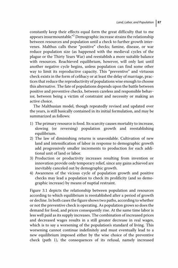
Land, Labor, and Population 87
constantly keep their effects equal form the great difficulty that to me appears insurmountable.”2 Demographic increase strains the relationship between resources and population until a check to further growth intervenes. Malthus calls these “positive” checks; famine, disease, or war reduce population size (as happened with the medieval cycles of the plague or the Thirty Years War) and reestablish a more suitable balance with resources. Reachieved equilibrium, however, will only last until another negative cycle begins, unless population can find some other way to limit its reproductive capacity. This “preventive” and virtuous check exists in the form of celibacy or at least the delay of marriage, practices that reduce the reproductivity of populations wise enough to choose this alternative. The fate of populations depends upon the battle between positive and preventive checks, between careless and responsible behavior, between being a victim of constraint and necessity or making an active choice.
The Malthusian model, though repeatedly revised and updated over the years, is still basically contained in its initial formulation, and may be summarized as follows:
1) The primary resource is food. Its scarcity causes mortality to increase, slowing (or reversing) population growth and reestablishing equilibrium.
2) The law of diminishing returns is unavoidable. Cultivation of new land and intensification of labor in response to demographic growth add progressively smaller increments to production for each additional unit of land or labor.
3) Production or productivity increases resulting from invention or innovation provide only temporary relief, since any gains achieved are inevitably canceled out by demographic growth.
4) Awareness of the vicious cycle of population growth and positive checks may lead a population to check its prolificity (and so demographic increase) by means of nuptial restraint.
Figure 3.1 depicts the relationship between population and resources according to which equilibrium is reestablished after a period of growth or decline. In both cases the figure shows two paths, according to whether or not the preventive check is operating. As population grows so does the demand for food, and prices consequently rise. At the same time labor is less well paid as its supply increases. The combination of increased prices and decreased wages results in a still greater decrease in real wages, which is to say a worsening of the population’s standard of living. This worsening cannot continue indefinitely and must eventually lead to a new equilibrium imposed either by the wise choice of the preventive check (path 1), the consequences of its refusal, namely increased
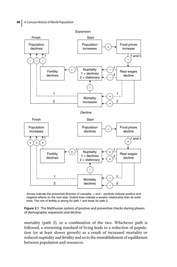
A Concise History of World Population88
mortality (path 2), or a combination of the two. Whichever path is followed, a worsening standard of living leads to a reduction of population (or at least slower growth) as a result of increased mortality or reduced nuptiality and fertility and so to the reestablishment of equilibrium between population and resources.
StartFinish
Expansion
Decline
Populationincreases
Populationincreases
Fertilitydeclines
Fertilitydeclines
Nuptiality1 = declines
2 = stationary
Nuptiality1 = declines
2 = stationary
Populationdeclines
Food pricesincrease
1 and 2
1 and 2
Real wagesdecline
Real wagesdecline
Mortalityincreases
Mortalitydeclines
Arrows indicate the presumed direction of causality, + and – symbols indicate positive andnegative effects on the next step. Dotted lines indicate a weaker relationship than do solidlines. The role of fertility is strong for path 1 and weak for path 2.
Start
Populationdeclines
Food pricesdecline
Finish
1
1
1
– – –
+
+
+
+
+
+
+ + +
+
–
–
–
–
–
–
–
––
2
2
1
2
1
2
1
2
1
1
1
2
1
Figure 3.1 The Malthusian system of positive and preventive checks during phases of demographic expansion and decline.
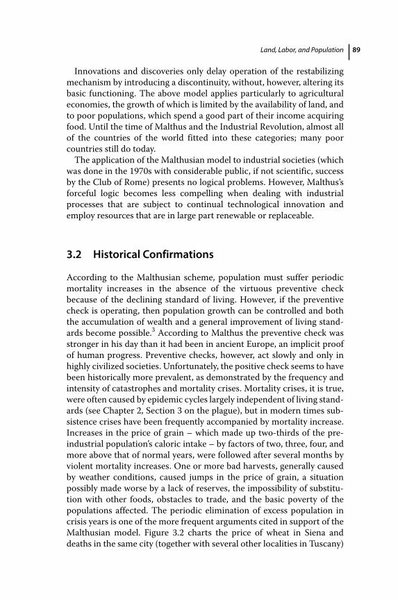
Land, Labor, and Population 89
Innovations and discoveries only delay operation of the restabilizing mechanism by introducing a discontinuity, without, however, altering its basic functioning. The above model applies particularly to agricultural economies, the growth of which is limited by the availability of land, and to poor populations, which spend a good part of their income acquiring food. Until the time of Malthus and the Industrial Revolution, almost all of the countries of the world fitted into these categories; many poor countries still do today.
The application of the Malthusian model to industrial societies (which was done in the 1970s with considerable public, if not scientific, success by the Club of Rome) presents no logical problems. However, Malthus’s forceful logic becomes less compelling when dealing with industrial processes that are subject to continual technological innovation and employ resources that are in large part renewable or replaceable.
3.2 Historical Confirmations
According to the Malthusian scheme, population must suffer periodic mortality increases in the absence of the virtuous preventive check because of the declining standard of living. However, if the preventive check is operating, then population growth can be controlled and both the accumulation of wealth and a general improvement of living standards become possible.3 According to Malthus the preventive check was stronger in his day than it had been in ancient Europe, an implicit proof of human progress. Preventive checks, however, act slowly and only in highly civilized societies. Unfortunately, the positive check seems to have been historically more prevalent, as demonstrated by the frequency and intensity of catastrophes and mortality crises. Mortality crises, it is true, were often caused by epidemic cycles largely independent of living standards (see Chapter 2, Section 3 on the plague), but in modern times subsistence crises have been frequently accompanied by mortality increase. Increases in the price of grain – which made up two‐thirds of the preindustrial population’s caloric intake – by factors of two, three, four, and more above that of normal years, were followed after several months by violent mortality increases. One or more bad harvests, generally caused by weather conditions, caused jumps in the price of grain, a situation possibly made worse by a lack of reserves, the impossibility of substitution with other foods, obstacles to trade, and the basic poverty of the populations affected. The periodic elimination of excess population in crisis years is one of the more frequent arguments cited in support of the Malthusian model. Figure 3.2 charts the price of wheat in Siena and deaths in the same city (together with several other localities in Tuscany)
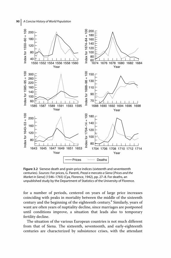
A Concise History of World Population90
for a number of periods, centered on years of large price increases coinciding with peaks in mortality between the middle of the sixteenth century and the beginning of the eighteenth century.4 Similarly, years of want are often years of nuptiality decline, since marriages are postponed until conditions improve, a situation that leads also to temporary fertility decline.
The situation of the various European countries is not much different from that of Siena. The sixteenth, seventeenth, and early‐eighteenth centuries are characterized by subsistence crises, with the attendant
40
60
8080
1704 1706 1708 1710 1712 1714
100
120
140
180
1643 1645 1647 1649 1651 1653
120
160
200
70
90
110
130
150
1585 1587 1589 1591 1593 1595
100140160220260300
601674
1688 1690 1692 1694 1696 1698
1676 1678 1680 1682 16841550 1552 1554 1556Year
Year
Year
Year
Year
Year
1558 1560
80
Inde
x fo
r 15
50–6
0 =
100
Inde
x fo
r 15
85–9
5 =
100
Inde
x fo
r 16
43–5
3 =
100
Inde
x fo
r 17
04–1
4 =
100
Inde
x fo
r 16
88–9
8 =
100
Inde
x fo
r 16
74–8
4 =
100
120
180
200
80
120100
180160140
200
DeathsPrices
Figure 3.2 Sienese death and grain‐price indices (sixteenth and seventeenth centuries). Sources: For prices, G. Parenti, Prezzi e mercato a Siena [Prices and the Market in Siena] (1546–1765) (Cya, Florence, 1942), pp. 27–8. For deaths, an unpublished study by the Department of Statistics of the University of Florence.
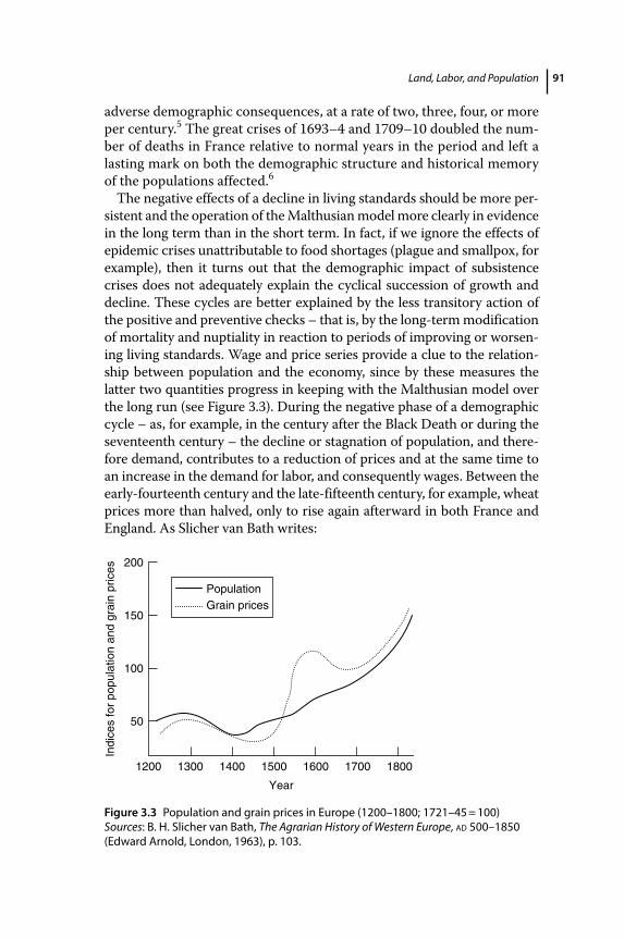
Land, Labor, and Population 91
adverse demographic consequences, at a rate of two, three, four, or more per century.5 The great crises of 1693–4 and 1709–10 doubled the number of deaths in France relative to normal years in the period and left a lasting mark on both the demographic structure and historical memory of the populations affected.6
The negative effects of a decline in living standards should be more persistent and the operation of the Malthusian model more clearly in evidence in the long term than in the short term. In fact, if we ignore the effects of epidemic crises unattributable to food shortages (plague and smallpox, for example), then it turns out that the demographic impact of subsistence crises does not adequately explain the cyclical succession of growth and decline. These cycles are better explained by the less transitory action of the positive and preventive checks – that is, by the long‐term modification of mortality and nuptiality in reaction to periods of improving or worsening living standards. Wage and price series provide a clue to the relationship between population and the economy, since by these measures the latter two quantities progress in keeping with the Malthusian model over the long run (see Figure 3.3). During the negative phase of a demographic cycle – as, for example, in the century after the Black Death or during the seventeenth century – the decline or stagnation of population, and therefore demand, contributes to a reduction of prices and at the same time to an increase in the demand for labor, and consequently wages. Between the early‐fourteenth century and the late‐fifteenth century, for example, wheat prices more than halved, only to rise again afterward in both France and England. As Slicher van Bath writes:
50
1200 1300 1400
PopulationGrain prices
1500
Year
1600 1700 1800
100
Indi
ces
for
popu
latio
n an
d gr
ain
pric
es
150
200
Figure 3.3 Population and grain prices in Europe (1200–1800; 1721–45 = 100) Sources: B. H. Slicher van Bath, The Agrarian History of Western Europe, ad 500–1850 (Edward Arnold, London, 1963), p. 103.
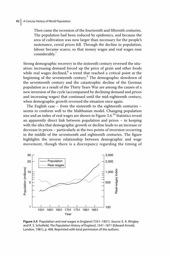
A Concise History of World Population92
Then came the recession of the fourteenth and fifteenth centuries. The population had been reduced by epidemics, and because the area of cultivation was now larger than necessary for the people’s sustenance, cereal prices fell. Through the decline in population, labour became scarce, so that money wages and real wages rose considerably.7
Strong demographic recovery in the sixteenth century reversed the situation: increasing demand forced up the price of grain and other foods while real wages declined,8 a trend that reached a critical point at the beginning of the seventeenth century.9 The demographic slowdown of the seventeenth century and the catastrophic decline of the German population as a result of the Thirty Years War are among the causes of a new inversion of the cycle (accompanied by declining demand and prices and increasing wages) that continued until the mid‐eighteenth century, when demographic growth reversed the situation once again.
The English case – from the sixteenth to the eighteenth centuries – seems to conform well to the Malthusian model. Changing population size and an index of real wages are shown in Figure 3.4.10 Statistics reveal an apparently direct link between population and prices – in keeping with the idea that demographic growth or decline leads to an increase or decrease in prices – particularly at the two points of inversion occurring in the middle of the seventeenth and eighteenth centuries. The figure highlights the inverse relationship between demographic and wage movement, though there is a discrepancy regarding the timing of
5
11551 1601 1651 1701
Year1751 1801 1851
100
500
Rea
l-wag
es in
dex
1,000
2,000
3,000
Population
Pop
ulat
ion
(mill
ions
) Real wages
10
20
30
Figure 3.4 Population and real wages in England (1551–1851). Source: E. A. Wrigley and R. S. Schofield, The Population History of England, 1541–1871 (Edward Arnold, London, 1981), p. 408. Reprinted with kind permission of the authors.
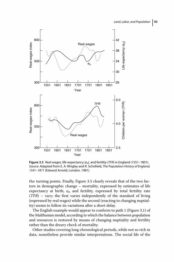
Land, Labor, and Population 93
the turning points. Finally, Figure 3.5 clearly reveals that of the two factors in demographic change – mortality, expressed by estimates of life expectancy at birth, e0, and fertility, expressed by total fertility rate (TFR) – vary; the first varies independently of the standard of living (expressed by real wages) while the second (reacting to changing nuptiality) seems to follow its variations after a short delay.
The English example would appear to conform to path 1 (Figure 3.1) of the Malthusian model, according to which the balance between population and resources is restored by means of changing nuptiality and fertility rather than the dreary check of mortality.
Other studies covering long chronological periods, while not so rich in data, nonetheless provide similar interpretations. The social life of the
1551300
500
Rea
l-wag
es in
dex
Rea
l-wag
es in
dex
800
300
500
800
1601 1651 1701Year
Real wages
1751 1801 1851
1551 1601 1651 1701
e0
Real wages
Year
1751 1801 185126
30
34
Life
exp
ecta
ncy
(e0)
38
42
2.5
4.0C
hild
ren
per
wom
an (
TFR
)6.0TFR
Figure 3.5 Real wages, life expectancy (e0), and fertility (TFR) in England (1551–1801). Source: Adapted from E. A. Wrigley and R. Schofield, The Population History of England, 1541–1871 (Edward Arnold, London, 1981).
A Concise History of World Population94
area of Languedoc in southern France is characterized by marked economic–demographic cycles.11 A first cycle was completed prior to the plague of 1348. As in much of Europe, population expanded and marginal land – rugged and not very productive – was progressively settled. Signs of frequent famine and demographic slowdown are evident at the end of the thirteenth and in the first half of the fourteenth centuries, followed by plague and population decline. This decline had several sociodemographic effects – for example, the recombination of family nuclei into extended families and land redistribution, both suited to an agricultural system suddenly rich in land and poor in labor. The most significant economic effect for our purposes, however, was the reduction of prices and the increase in wages until demographic recovery gained momentum and accelerated in the sixteenth century. Once again land became scarce; new and progressively less productive land was tilled; real wages declined; society became poorer; and, in the period spanning the seventeenth and eighteenth centuries, population declined. Le Roy Ladurie interprets these alternating cycles of growth and decline in Malthusian terms. Population grows more rapidly than resources, and in the long run, in the absence of technological improvements, positive checks intervene. The case of Languedoc differs from that of England in that it follows path 2 of Figure 3.1, according to which mortality is the regulating mechanism.
Similar interpretations exist for other regions of both southern and northern Europe.12 Common to all of these is the observation that demographic growth and the process of diminishing returns lead to a decline in per capita production and so increase poverty and that this spiral, or “trap,” can be avoided or at least attenuated by innovation or by the control of demographic growth.
3.3 Demographic Pressure and Economic Development
The logic of diminishing returns implies a continual contest between the growth of resources and population, unless the latter is controlled by reproductive restraint and so permits the accumulation of wealth and increased well‐being. Demographic growth, in any case, acts as a check to economic development.
The opposing theory to that of Malthus, according to which population increase stimulates development, has an even longer history. Economists of the seventeenth century, and much of the eighteenth century, worried by the negative economic effects associated with the depopulation of a number of countries (especially Spain and Germany)
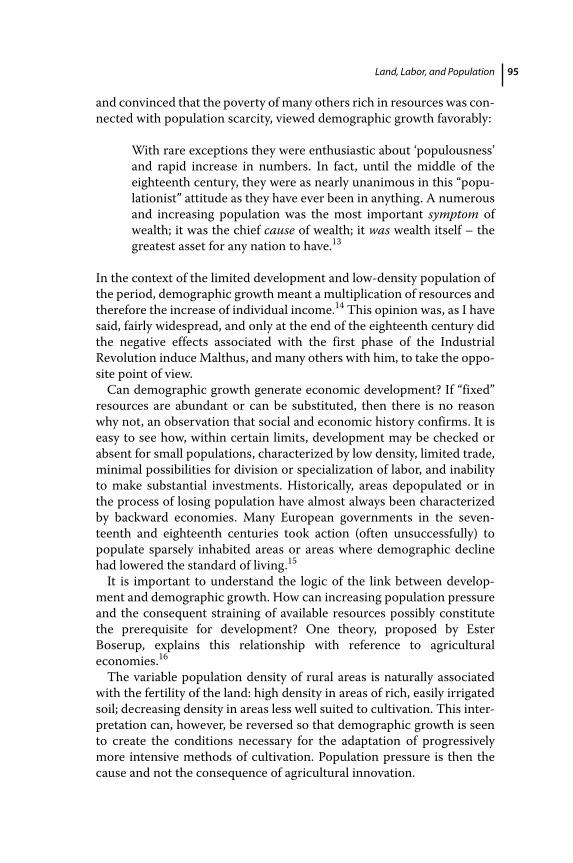
Land, Labor, and Population 95
and convinced that the poverty of many others rich in resources was connected with population scarcity, viewed demographic growth favorably:
With rare exceptions they were enthusiastic about ‘populousness’ and rapid increase in numbers. In fact, until the middle of the eighteenth century, they were as nearly unanimous in this “populationist” attitude as they have ever been in anything. A numerous and increasing population was the most important symptom of wealth; it was the chief cause of wealth; it was wealth itself – the greatest asset for any nation to have.13
In the context of the limited development and low‐density population of the period, demographic growth meant a multiplication of resources and therefore the increase of individual income.14 This opinion was, as I have said, fairly widespread, and only at the end of the eighteenth century did the negative effects associated with the first phase of the Industrial Revolution induce Malthus, and many others with him, to take the opposite point of view.
Can demographic growth generate economic development? If “fixed” resources are abundant or can be substituted, then there is no reason why not, an observation that social and economic history confirms. It is easy to see how, within certain limits, development may be checked or absent for small populations, characterized by low density, limited trade, minimal possibilities for division or specialization of labor, and inability to make substantial investments. Historically, areas depopulated or in the process of losing population have almost always been characterized by backward economies. Many European governments in the seventeenth and eighteenth centuries took action (often unsuccessfully) to populate sparsely inhabited areas or areas where demographic decline had lowered the standard of living.15
It is important to understand the logic of the link between development and demographic growth. How can increasing population pressure and the consequent straining of available resources possibly constitute the prerequisite for development? One theory, proposed by Ester Boserup, explains this relationship with reference to agricultural economies.16
The variable population density of rural areas is naturally associated with the fertility of the land: high density in areas of rich, easily irrigated soil; decreasing density in areas less well suited to cultivation. This interpretation can, however, be reversed so that demographic growth is seen to create the conditions necessary for the adaptation of progressively more intensive methods of cultivation. Population pressure is then the cause and not the consequence of agricultural innovation.
A Concise History of World Population96
The various systems of land cultivation spread across a continuum that stretches from forest‐fallow systems (slash‐and‐burn preparation of the terrain followed by 1 or 2 years of cultivation, and then a long fallow period of 20–25 years during which the forest reestablishes itself and the fertility of the soil is restored) at one end to multiannual cropping on the same piece of land at the other. Between the two extremes brush‐fallow cultivation is identical in method to forest‐fallow, but shorter, as a covering of shrubs reestablishes itself after 6 to 8 years. In a short‐fallow system (1 or 2 years) there is only time for a grassy covering to grow back, while annual cropping allows but a few months for the soil to rest. Demographic growth determines the transition to progressively more intensive and shorter fallow cultivation systems that permit the feeding of a progressively larger population in a fixed area. This intensification process, however, is accompanied by an ever greater labor requirement and often also by declining worker productivity. For example, land preparation and the sowing of seed are extremely rudimentary in a slash‐and‐burn system: hatchet and fire clear the terrain of forest, ash fertilizes the soil, a pointed stick is all that is needed to sow the soft earth, and productivity per hour of work is high. Shorter fallow periods require more laborious soil preparation, and the simple action of fire must be replaced by work with hoe or plow; fertilization, weeding, and irrigation all become necessary. In a forest‐fallow system,
fire does most of the work and there is no need for the removal of roots, which is such a time‐consuming task when land has to be cleared for the preparation of permanent fields. The time used for superficial clearing under the system of forest fallow therefore seems to be only a fraction – perhaps ten or twenty per cent – of the time needed for complete clearing.17
Tools, also, change at the various stages: while a pointed stick suffices for the sowing of seed in a slash‐and burn‐system, a hoe is needed to clear the soil of shrub when fallow is shorter and a plough to eradicate weeds when it is shorter still. When animal power is introduced for plowing, the livestock produce fertilizer, but at the same time must be fed and cared for, tasks requiring additional labor. In order to obtain the same product, each farmer must work longer; in other words, his productivity per hour worked (in the absence of technological innovations) tends to decline. When population becomes too large in relation to available land, farmers are forced to use new techniques which, by virtue of increased inputs of labor, allow for greater production per unit of land. In many cases, so goes the argument, certain populations do not adopt more intensive techniques not because they are unaware of these alternatives but
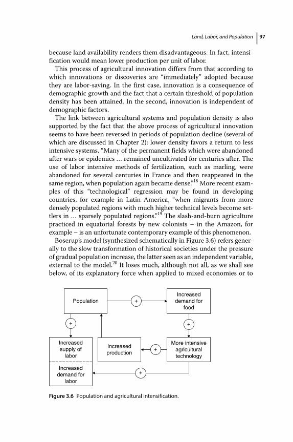
Land, Labor, and Population 97
because land availability renders them disadvantageous. In fact, intensification would mean lower production per unit of labor.
This process of agricultural innovation differs from that according to which innovations or discoveries are “immediately” adopted because they are labor‐saving. In the first case, innovation is a consequence of demographic growth and the fact that a certain threshold of population density has been attained. In the second, innovation is independent of demographic factors.
The link between agricultural systems and population density is also supported by the fact that the above process of agricultural innovation seems to have been reversed in periods of population decline (several of which are discussed in Chapter 2): lower density favors a return to less intensive systems. “Many of the permanent fields which were abandoned after wars or epidemics … remained uncultivated for centuries after. The use of labor intensive methods of fertilization, such as marling, were abandoned for several centuries in France and then reappeared in the same region, when population again became dense.”18 More recent examples of this “technological” regression may be found in developing countries, for example in Latin America, “when migrants from more densely populated regions with much higher technical levels become settlers in … sparsely populated regions.”19 The slash‐and‐burn agriculture practiced in equatorial forests by new colonists – in the Amazon, for example – is an unfortunate contemporary example of this phenomenon.
Boserup’s model (synthesized schematically in Figure 3.6) refers generally to the slow transformation of historical societies under the pressure of gradual population increase, the latter seen as an independent variable, external to the model.20 It loses much, although not all, as we shall see below, of its explanatory force when applied to mixed economies or to
PopulationIncreased
demand forfood
More intensiveagriculturaltechnology
Increasedproduction
+
+
+
+
+
Increasedsupply of
labor
Increaseddemand for
labor
Figure 3.6 Population and agricultural intensification.
A Concise History of World Population98
developing countries experiencing modern demographic acceleration. This model does not rule out the operation of other factors, but posits demographic growth as one of the driving forces of economic transformation. It overturns the Malthusian model as population becomes not a variable dependent upon development but one that itself determines that development.
3.4 More on Demographic Pressure and Development: Examples from the Stone Age to the Present Day
The positive theory of demographic pressure has been applied, with intriguing results, to the “rapid” transition from hunting and gathering to agriculture, which I discussed earlier. This transition allowed the human race – which for hundreds of thousands of years had depended on those animal and vegetable products supplied spontaneously by the ecosystem – to develop, in just a few thousand more, a system for the man‐made production of resources.
According to the traditional theory, this transition is explained by the development and diffusion of innovations and inventions. The invention of new techniques of animal domestication, planting, and harvesting led to increased and more stable production and so provoked demographic acceleration.21 In other words, people modified the environment and so established the conditions for population growth. Mark Cohen, like Boserup, turns the process around.22 When, 11,000 to 12,000 years ago, hunter‐gatherer societies had settled all the land then available, demographic growth forced them to enlarge their range of gathering to include inferior foods that were less nutritional and lacking in flavor. Then, beginning 9,000 years ago, hunter‐gatherers were forced to enlarge still further this range of food, cultivating not tastier foods but those easily reproduced, and so the transition to agriculture began. This argument is based on two primary arguments and a series of corollaries.
According to the first argument, agriculture consists of a series of practices and techniques that were known to hunter‐gatherers but not adopted because they were unnecessary:
Any human group dependent in some degree on plant materials, possessing the rudiments of human intelligence, and having any sort of home‐base camp structure … will be almost bound to observe the basic process by which a seed or shoot becomes a plant … Agriculture is … a combination of behaviors … including such things as the creation of clearings in which certain plants
Land, Labor, and Population 99
thrive; the enrichment of certain soils; the planting of seeds; the irrigation of plants; the removal of competing species; the practice of conservation measures; the transporting of species beyond their original ecological boundaries; or the selection of preferred types. None of these behaviors alone constitutes agriculture; taken together they are agriculture.23
The second argument involves the level of nutrition and the work required to obtain this level with the transition to agriculture. In the first place, this transition entailed a deterioration of both the quality and variety of diet, as the food acquired by fishing, hunting, and gathering is much richer in nutrition and flavor than that of sedentary agriculture, dominated by a monotony of grain. Consequently, this transition would not have been expedient in the absence of the demographic growth that made it necessary. In addition, the work of a sedentary farmer was considerably more onerous than that of a hunter‐gatherer, who often considered the search for food not so much a form of labor as a natural way of life.
This theory is based primarily on observations of groups of hunter‐gatherers that have survived to the present day. The hypothesis regarding the light workload entailed by this survival model is confirmed by the Bushmen of the Kalahari, among whom the adult males devote on average two or three hours a day to obtaining food, by the Arnhem Land Aborigines, who average three to five hours, and by the tribes of Tanzania, at barely two.24 Similar observations were made in the nineteenth century by Grey.25 Comparisons between primitive farmers and their hunter‐gatherer predecessors presumably also confirm the lesser effort exerted by the hunter‐gatherers for acquiring adequate food. In conclusion, “agriculture permits denser food growth supporting denser populations and larger social units, but at the cost of reduced dietary quality, reduced reliability of harvest, and equal or probably greater labor per unit food.”26 Agriculture spreads, then, when demographic growth requires greater production per unit area. Keeping in mind the fact that there existed a rebalancing mechanism (migration), which distributed excess population among areas thereby reducing demographic pressure, one can understand why the transition to agriculture (driven by demographic growth) took place in a relatively short period of time as compared to the duration of human history.
Cohen’s approach has provoked intense debate and many attempts at confirmation. In particular, attention has been focused on the hypothesis that the period leading up to agricultural transition was characterized by a decline in living standards and nutritional levels. Confirmation, however, remains elusive, and both archaeological finds and paleopathological studies are inconclusive on this point.27
A Concise History of World Population100
The theory according to which the first known demographic revolution led to the invention of agriculture shares, with that of Boserup, the belief that population acts as a stimulus to development. Later demographic developments – the period of growth in medieval Europe prior to the plague, for example – also provoked changes in the organization of production in keeping with the above model.
The new system, which spread in the period between the ninth and fourteenth centuries, was a three‐course rotation of all the fields in a village, in which two cereal crops were followed by 1 year of fallow. The stubble and fallow were utilized for supervised grazing by domestic animals belonging to all the villagers. Stubble‐grazing animals fertilized the fields with their droppings, helping to compensate for loss of soil fertility by shorter fallowing, and for loss of natural pastures due to expansion of the cultivated area. Even so, it is possible that crop yields were lower than they had been under the long‐fallow system, and it is likely that there was some shift of diet from animal to vegetable food as population continued to increase. When the Black Death later reduced population densities, an opposite shift to less vegetable food took place, as arable fields, made superfluous by the decline of population, returned to pasture.28
In the Low Countries – the most densely settled area of Europe – the agricultural system was able to avoid the recurrent bouts of famine and starvation typical of other parts of Europe. And it is in the Low Countries, according to Boserup, that major innovations such as short fallows and root crops with high caloric content per unit of land were first introduced.
Evidence from present‐day agricultural societies using traditional techniques also confirms the theory of the propulsive role of demographic growth. For instance, between 1962 and 1992, in the developing countries, a positive association has been found between changes in labor/land ratios (generally increasing) and land productivity, also on the increase. Population pressure on land has increased in most countries, determining a Boserupian response of augmented land yields. An influential study employs a series of cases taken from Latin America, Africa, and Asia in the period 1962–92.29 In these, the level of population pressure has been much greater than in the past owing to higher rates of growth. The cases analyzed illustrate the response of agricultural societies to growth rates of 2–3 percent per year; in almost all cases urban growth has absorbed a fraction of rural demographic excess (or excess rural population), and in some the nonagricultural sector has actually come to dominate.
Land, Labor, and Population 101
Given approximately equal technological levels, the work required for the cultivation of a given crop on a given unit of land increases with increasingly intensive cultivation systems. For example, comparing forest‐fallow cultivation – employing the slash‐and‐burn technique and long fallow periods – to annual cultivation, the yearly total of hours worked per hectare jumps from 770 to 3,300 in Cameroon.30 The increased labor requirement is the result of both the greater amount of work needed for each phase of cultivation (preparation of the soil, weeding, and so forth) and the larger number of phases (irrigation and fertilization, for example). Three operations are sufficient for slash‐and‐burn agriculture: preparation of the soil by burning, which requires 300–400 hours per hectare in Liberia or the Ivory Coast; planting with a stick or hoe in the fire‐softened terrain; and harvesting. Virtually no work is performed in the period between sowing and harvesting, since no fertilization, weeding, or irrigation are required. As cultivation intensifies, the latter operations become indispensable and progressively more laborious. Considering all 52 of the cases studied by Pingali and Binswagen, and calculating indices of cultivation and labor intensity,31 one notes a positive correlation between the two variables: a 10 percent increase in cultivation intensity corresponds on average to a 4.6 percent increase in hours worked per hectare. The same analysis reveals that the 10 percent increase in cultivation intensity corresponds to a 3.9 percent increase in production per hectare. Productivity per hour worked, then, declines slightly, but if we also take into account the work hours not strictly employed in cultivation (such as the raising and care of livestock and the maintenance of irrigation systems and of tools), the decline in productivity per hour worked is greater. This productivity decline (calculated in the absence of innovations) can, of course, be compensated for by sufficient investment and by new technology.
The experience of developing countries confirms many aspects of the theory. Agricultural intensification implies more work per unit of cultivated terrain and, given a constant level of technology, more work per unit of production. This trend has been effectively countered in recent history by technological innovation, but it is conceivable that in earlier epochs, when the pace of such innovation was either slow or static, the adoption of new methods of cultivation came about as a result of necessity and at the price of greater workloads.
3.5 Space, Land, and Development
For much of human history, the well‐being of a population has depended upon the availability of space and land, and on the constraints imposed by their lack or limited supply. The ways in which populations have
A Concise History of World Population102
succeeded in overcoming or sidestepping these constraints by means of innovation and adaptation have been the leading determinants of survival and growth. The models described above, whether Malthusian or Boserupian, depend on space; in the first case primarily as a determining factor of demographic change and in the second as a dimension that responds to and is altered by population growth or decline. In the course of the history of population, these models have alternated, overlapped, and intersected; nor is it easy to make out their separate influences. In order to study long‐term demographic growth, we must take “space” into account and all that it implies, in particular land, the products of the land (food, manufactured goods, energy), and those characteristics that determine settlement patterns. Demography has for too long ignored, or at best paid scant attention to, these themes and so deprived itself of valuable interpretative tools. Indeed the relevance of space for the understanding of demographic trends should be both directly and indirectly evident throughout this book, whether in relation to the Neolithic revolution, the settlement of new territories, or the events in Ireland and Japan.
One major aspect of the interaction between land, space, and development concerns migration. Current narrative has it that our species moved out of Africa to western Asia and Europe, then to eastern Asia and reached, in the final phase of its dispersion, America and Oceania,32 a process of dispersion and settlement through migration into territories either empty or settled by other humans (like Neanderthals in Europe) with less developed abilities. The first Siberian hunters who ventured eastward, during the last glaciation, on the firm land bridge that emerged between Asia and America, more than 20,000 years ago, were the vanguard of a long and slow march moving from Alaska to the Tierra del Fuego. According to some scholars, the occupation of the entire continent, from the extreme north to southernmost part, took place in a relatively short period of time, of the order of a few thousand years.33
More specific considerations can be made with reference to the Neolithic revolution and the rise of agriculture in the near East and Europe. It is a process that initiated 9,000 years ago, originating in the near East, and terminated some 5,000 years ago in the British Isles. Two explicative theories are on the table, but they are not mutually exclusive, because a combination of the two is possible. One theory holds that the rise of agriculture is the consequence of a process of cultural diffusion. Knowledge, techniques, and practices travel through space from one group to another through communication, learning, and adoption. For the other theory, which we can name “demic diffusion,” the agriculturalists travel and migrate pushed by a robust demographic growth and take along their techniques and practices. The combination of demographic
Land, Labor, and Population 103
growth and propensity to migrate is the origin of a “diffusion wave,” slow but continuous.34
This form of slow and gradual migration, this “diffusion wave,” typical of agriculturalists in empty or sparsely populated spaces, had two characteristics. The first relates to the ability of moving and adapting to different environments that are not always more favorable than the ones left behind. The ability to adapt was probably a function of the capital of knowledge and experience, of technical abilities, of ownership of tools: the higher the endowment, the better the ability to exploit the potentialities of the new settled territories. The second characteristic was the possibility, for families and communities settled in front of the wave, to generate a demographic surplus sufficient to fuel further advances. Both migration and adaptation are closely tied to selective processes. There are historical proofs that migrants are not a random sample of the original population but are selected for several characteristics. Age, health, physical strength, endurance, and inclination for new experiences are qualities of which the migrant population and the original settled group have different endowments. All this is largely conjectural for prehistorical populations, less so for the historical ones.
In order to discuss the relationships between space and demography, let us take Europe as an example, a continent – or perhaps more appropriately the western extension of the large Eurasian continent – for which we have access to abundant information. It is a continent marked by at least three fundamental characteristics. The first is its relatively easy access; it is almost entirely surrounded by sea, is penetrated by numerous waterways, and includes important orographic features that regulate but do not prevent communications. The second is its favorable climate, for the most part temperate and supportive of a wide range of crops. The third is the great variability of its environmental conditions that require adaptation on the part of the populations but at the same time favor specialization.
The area of Europe (taken to extend to the Urals, the Caspian Sea, and the Caucasus) measures 9.6 million km2, of which about half belongs to Russia. It would be superficial in this context to examine the complex relations between space and population in such a vast and varied area, though there are many interesting points to be made. According to Cavalli‐Sforza and Ammerman, it was because of the availability of space that agriculturalists progressively migrated northwest from Asia Minor to Europe, bringing new settlement and cultivation techniques and either causing or at least encouraging the Neolithic revolution there. Similarly, the increasing pressure exerted by nomadic peoples against the eastern borders of the Roman Empire must be ascribed to the conquest of space and resources.
A Concise History of World Population104
In order to understand the relationship between space and demographic change better, at least three processes of analysis need to be investigated. The first concerns the occupation of uninhabited or sparsely populated regions within a settled area; the second the transformation of existing space by means of deforestation, land reclamation, and swamp draining; and the third the expansion outside settled areas through emigration and the colonization of new territories. These three processes are intimately linked and can conceptually be put in chronological order (though in fact they can all happen at the same time) according to the growing economic, social, and human costs they require.
3.5.1 The occupation of uninhabited or sparsely populated regions
This sort of expansion accompanied the medieval demographic growth of the eleventh to thirteenth centuries, a period during which European population multiplied by a factor of two or three. According to Grigg, “In ad 900 much of Europe was covered by forest, but the following centuries saw the removal of woodland to allow cultivation. Between ad 1000 and 1300 much of the lowland forest was removed in central and western Europe, and cultivation also extended into mountain areas, notably in the Vosges, Alps and Pyrenees.”35 It was a widespread process as already settled territories were expanded by means of the cultivation of new land, often accompanied by the consolidation of population in towns, castles, and new cities.36 The expansion of cultivated land came about in varied ways, though in the majority of cases it was the individual peasant who plowed open space bordering already cultivated fields or else cleared woodland. In other cases new settlements were organized by landlords.37 This process is a well‐documented one, in Italy, Spain, France, Germany, and elsewhere. Obviously, the increasing demands for resources made by an expanding population were also satisfied to some extent by land reclamation, settlement at higher elevations, and costly land transformations (within the limits of available technology and usually by means of that intensification of agriculture we have already discussed). Still, it is hard to imagine that medieval expansion would have been as dynamic as it was without an abundance of easily acquired land.
3.5.2 Transformation and land reclamation
At considerably higher cost, land reclamation helped to sustain medieval population growth. Dams were built to control stream waters and to protect lowlands from flooding by both rivers and the sea: “Coastal areas saw much reclamation, and embankments were built to protect low‐lying land both from the sea and from estuarine flooding in Lincolnshire and
Land, Labor, and Population 105
Norfolk, on the Elbe, the Loire, the coast of Flanders, and most notably in the Zuiderzee.”38 Similar hydraulic work was carried out in the Po Valley, including projects financed by cities in Lombardy, Emilia, Romagna, and in the Venetian plain.39
Land reclamation took on larger proportions during the demographic recovery that followed the crisis of the fourteenth and fifteenth centuries. In England wet and swampy areas, both internal (in Lancashire and in the Fenlands) and along the coasts of Sussex, Norfolk, and Essex, were drained.40 Similar work was carried out in France, along the northern coast with the help of Dutch workers and also in the south along the malarial and swampy coasts of Provence and Languedoc.41 In Italy reclamation activity took off again as well:
all of the lower Po Valley was affected by the great reclamation movement in the sixteenth century. To the west the first rice paddies were created in the eastern part of Piedmont between Novara and Vercelli, but the greatest activity was in the east; massive and surprising transformations took place on either side of the Po: in the Venetian terra firma, in the Duchies of Parma, Reggio, Mantua, and Ferrara, and in Emilia.42
Yet it was in the Netherlands, in response to population growth and the increase in grain prices between the late‐fifteenth and mid‐seventeenth centuries that the reclamation of land from sea and marsh by means of dikes, canals, and pump‐works took on formidable dimensions. “Between 1540 and 1565, 125,000 hectares of polders were diked; one‐half of this was in Zeeland and North Brabant, one‐third in the Netherlands, the remaining sixth in Friesland and Groningen.”43 There were also reclaimed lands in the interior of the country: “The area brought into cultivation was remarkable: between 1550 and 1650 the population of the Netherlands increased by some 600,000 but the area reclaimed was some 162,000 hectares.”44 If we assume that one hectare can sustain on average two or three people, then the added land would have fed between one‐half and three‐quarters of the added population. In the Netherlands land reclamation followed demographic growth apace. Elsewhere the demographic awakening of the second half of the eighteenth century was accompanied by the revival of reclamation projects as well: in England and Ireland, Poitou and Provence, Schleswig‐Holstein and Prussia, and Catalonia and the Italian Maremma.
3.5.3 External Expansion
The third element in the complex relationship between space and population is the existence of accessible space outside already‐settled areas.
A Concise History of World Population106
Europe has been both a receiver and a supplier of population in this regard. Prior to the Middle Ages, population flowed in from the steppes to the east and the Mediterranean to the south. In the period since the Middle Ages it would be difficult to understand the development of European demography and society without taking into account the availability of inhabitable spaces to the west and east and so the phenomena of emigration and colonization. The accessibility of these spaces and the force of attraction they exert is one of the two major factors behind the great migrations; the other is the existence of forces of expulsion tied to economic difficulties in the sending regions. We shall discuss at greater length later the great nineteenth‐century transoceanic migrations, which took place in a period of rapid economic and industrial change, but, for the moment let us restrict our attention to Europe between the Middle Ages and the Industrial Revolution and focus on three great movements. The first is the German colonization of the territory east of the Elbe River between the eleventh and the fourteenth centuries. The second includes the Iberian migration to Central and South America and the British migration to North America as well as the relatively minor movements of the Dutch and the French to their respective colonies in the period from the sixteenth to the eighteenth centuries; these movements constitute the prelude to the great migrations of the nineteenth century. The third is the expansion of the Russian frontier to the east and to the south.
The drive to the east – Drang nach Osten – was a phenomenon of great proportions as it determined the peopling of large areas east of the Elbe and then successively of Poland, the Sudetenland, and Transylvania. It was a colonization process begun in the twelfth century by Dutch and Flemish pioneers – in part organized, in part spontaneous – who moved into open areas sparsely inhabited by Slavs. It is estimated that this migration involved 200,000 people who, in the course of the twelfth century, occupied the region between the Elbe and the Oder, and that the thirteenth‐century wave that helped populate Silesia and Pomerania was of a similar size. It was a relatively modest migratory flow but one of considerable importance in the long run: at the end of the nineteenth century the Germanic population east of the Elbe‐Saale line was about 30 million.45 In the eighteenth century, by calling on several tens of thousands of German colonists, Catherine the Great of Russia produced a new wave of migration into the valley of the Volga in an attempt to push the border southward. Between 1764 and 1768, 104 colonies were founded on the banks of the Volga for 27,000 immigrants. Other settlements in the Crimea, North Caucasus, Kazakhstan, and Siberia followed.46 From a demographic point of view, the interest of these migrations lies not so much in their size, which was modest in both absolute and relative terms, but in their makeup: the migrants were for the
Land, Labor, and Population 107
most part young workers, many without families; they represented a significant portion of the reproductive‐age population and so an outlet for demographic increase. Their progeny was considerable: as with the French Canadian pioneers (see Chapter 2, Section 5), their reproductivity was high, because of both the selective effects of migration and the abundance of available resources better exploited by large families. A few hundred thousand Germanic colonists, then, became, a few centuries later, tens of millions, and the few tens of thousands who migrated to Russia founded colonies that grew into large settlements by the end of the nineteenth century.
The second great migratory outlet was the American continent and, to a lesser extent, other overseas settlements. At the end of the eighteenth century, as the colonial system was collapsing, the American continent was home to modest but significant European settlements: about 4 million in Latin America and 4.5 in North America.47 These settlements, fed by migrations from Spain and the British Isles and to a lesser degree Portugal, were small in comparison to the physical dimensions of the continent but nonetheless constituted one‐third of its population. As compared to the population of Europe (excluding Russia) they amounted to only about one‐fifteenth.
On the basis of indirect estimates derived from maritime traffic, the Spanish contribution is thought to be 3,000–5,000 emigrants per year for the 150 years ending in the mid‐seventeenth century. They came almost exclusively from Castile and constituted a loss (according to the highest estimate) of 1 per 1,000 per year, a significant figure given their young age structure and the weak demographic growth of the period. After 1630, and in conjunction with the general (including demographic) crisis, emigration declined and reached a minimum between 1700 and 1720.48 The drain on England was greater, amounting to a net figure of 7,000 emigrants a year during the seventeenth century from a population that numbered little more than 4 million at its beginning.49 The emigration from the Netherlands was comparable to that from England; it is estimated that 230,000 net emigrants went to Asian locations between the beginning of the seventeenth century and the end of the eighteenth, to which were added 15,000 to Latin America and the Caribbean and 10,000 to the United States.50 France, the most populous country in Europe (see Chapter 2, Section 5), contributed relatively little to these migrations. Transoceanic migration between the beginning of the sixteenth century and the end of the eighteenth was numerically significant and constituted the demographic and political base for the great migrations of the nineteenth century; it made possible, then, an enormous expansion of European space beyond the Atlantic barrier that had enormous long‐term demographic consequences.
A Concise History of World Population108
The third movement consisted of the shift of the Russian border to the south and east. The peopling of Siberia in the nineteenth century – which takes us beyond the chronological limits here imposed – resembled that of the American continent, though the numbers were smaller. As McNeil writes:
By 1796, therefore, when the Empress Catherine II died, the Russian flood had engulfed the once‐formidable Tartar society … All the vast steppe region north of the Crimea and west of the Don had been occupied by landlords and settlers, and their political and social institutions had been effectively assimilated to those prevailing in the Russian empire as a whole … Yet new towns had arisen (Kherson, 1778; Nikolaev, 1788; Odessa, 1794) and throve as administrative centers and grain ports; and with urban life the manifestations of higher culture – flavored by a distinctly cosmopolitan tincture owing to admixture of Greeks, Bulgars, Poles, Jews, and a few western Europeans – soon appeared.51
These notes on an enormously complex and little‐known story should give some idea of the intimate relation between demographic change and the availability of space, whether internal or external, to the relevant populations. It is an argument with natural ties to the migrations that have traversed the continent in various directions. It helps us, in turn, to understand how in one millennium the availability of new spaces not strictly defined by political boundaries played a great and varied role in shaping demographic change. Space, then, has made possible the expansion of the European economy into a wider world.
3.6 Population Size and Prosperity
In the preceding pages I have discussed several possible dynamic relations between population and economic development. It is also worth taking a moment to consider the effect of the simple “number” of inhabitants on societal well‐being. I have already touched upon this argument in passing; it merits, however, something more than the observation that the level of complexity of social organization is also a function of numerical size. Many scholars have grappled with the question of whether there exists an “optimum” population size,52 but this academic exercise is not particularly helpful for understanding the historical reasons for demographic development. The concept of an optimum population, which may be defined as that theoretical population size at which individual well‐being is maximized (and above or
Land, Labor, and Population 109
below which well‐being declines), is an essentially static concept and applies poorly to dynamic populations.
Population size acts by means of two mechanisms well known to classical economists. The first is linked to the principle of division of labor and so to the more efficient use of individual abilities. The second derives from the observation that the complexity of societal organization is also a function of demographic dimensions, both absolutely and relative to a given unit of territory (density).
The benefits of division of labor were masterfully demonstrated by Adam Smith and before him by William Petty. Referring to the advantages of large cities, Petty wrote: “In the making of a Watch, If one Man shall make the Wheels, another the Spring, another shall Engrave the Dial‐plate, and another shall make the Cases, then the Watch will be better and cheaper, than if the whole Work be put upon any one Man.”53 Smith’s example of the blacksmith making nails and of the advantages to be gained from dividing up the work required for the production of pins is classic:
One man draws out the wire, another straights it, a third cuts it, a fourth points it, a fifth grinds it at the top for receiving the head, to make the head requires two or three distinct operations, to put it on is a peculiar business, to whiten the pins is another; it is even a trade by itself to put them into paper; and the important business of making a pin is, in this manner, divided into about eighteen distinct operations, which in some manufactories, are all performed by distinct hands.54
While a single worker might turn out at most 20 pins a day, a factory employing a team of 10 workers manages to produce 12 lb a day, or 48,000 pins, 4,800 per worker. Division of labor, however, is a function of the size of the market. If the market is small, division is moderate, as are the advantages to be gained. Smith observed that in the Highlands of his native Scotland, where families were widely scattered, each performed the tasks of butcher, baker, and brewer for itself. Smiths, carpenters, and masons were few, and those families 8 or 10 miles from town did much of this work themselves.55
Where it has been impossible to adequately divide labor, this situation has contributed in some measure to the backwardness of scattered groups; to the development difficulties encountered by small, isolated communities, the dimensions of which do not allow specialization; to the failure of colonization undertaken by small nuclei; and to the instability of small island populations even when the environment is favorable. The maximum of inefficiency according to this formula is that population consisting only of Robinson Crusoe.
A Concise History of World Population110
The second advantage to be gained from population size or density is the economy of scale acquired at increasing population levels. Better systems of resource utilization and production are only feasible when population attains a certain density in relation to the territory inhabited. We have already considered an example according to which the processes of agricultural intensification respond to the incitement of demographic growth. In our own time, a country like Canada is considered, by representatives of both the government and the citizenry at large, too “empty” to maintain that development that its extension and natural wealth would seem to ensure. Other classic examples include the development of irrigation systems, the establishment of cities, the improvement of communications, and, in general, those investments in infrastructure that require a critical mass of resources and a critical mass of demand – neither of which are obtainable from small groups and limited markets. These infrastructures can be developed at a lower cost per capita in a larger population.
The development of irrigation systems in Mesopotamia allowed the few hunter‐gatherers living in the Zagros Mountains in 8000 bce to evolve into a large population of plain dwellers in the following millennia.
This dense population used intensive systems of agriculture based upon flow irrigation; multicropping was also introduced. Fields were prepared by plows with moldboards and iron shares, drawn by oxen. The irrigation system used waterwheels for lifting water to fields located above the major river, which provided the water. Thus over a period of some eight thousand years, Mesopotamia became densely populated … Gradually, the population changed from primitive food gatherers to people who applied the most sophisticated systems of food production existing in the ancient world.56
The transformation of the Italian Maremma into swampland that accompanied the medieval population decline was a result of the reverse process that saw the deterioration of water control systems.
Considerations of this sort have also been applied to the development of road networks, which is strongly correlated to population density.57 Clearly the advantage and usefulness of a road is a function of how heavily it is traveled. Once built, it exerts multiple effects on development, speeding up communication, helping trade, and allowing the creation of a larger market. The differences in prices for basic goods in primitive societies are largely explained by difficulties of transportation and uncertain communications.
City growth, also, has obvious links to demography. I take for granted that the creation of cities allows for greater specialization and more
Land, Labor, and Population 111
efficient organization of the economy. While these advantages may well be compromised in the present day by the ever more evident “diseconomies” of scale created in the great urban centers, for the primarily rural economies that we are discussing the situation was altogether different. Clearly the maintenance of an important centralized population, not directly involved in food production, implies the creation of an agricultural surplus by the rural population; and the wealthier the latter, the greater the available resources. The early growth of cities in Mesopotamia, northern India, and China is certainly a function of the large populations allowed by the fertility of the land and agricultural abundance. It is once again Ester Boserup who provides an original explanation for this situation, proposing a causal chain: Demographic growth drives agricultural intensification, but it is not so much the level of per capita production – which increases with increasingly intensive cultivation – as it is increasing population density that allows for the creation of the surplus resources requisite for the birth of cities. More farmers within a given radius from the city imply a larger product and a larger surplus for support of a more numerous urban population.
Even the best technologies available to the ancient world, when used on the best land, did not allow one agricultural family to supply many nonagricultural families … The size of the population available to supply an urban center was far more important than how much food could be delivered or sold per agricultural worker.58
The links between division of labor, economies of scale, and demographic dimensions are easily grasped and demonstrated by numerous historical examples. Less easily demonstrated is another thesis, upheld by a number of scholars, which employs the following logical sequence: When resources are available, development is a function of what Kuznets calls “tested knowledge.”59 Employing a restrictive hypothesis, the “creators” of “new knowledge” (investors, innovators) exist in proportion to population size. The creation of “new knowledge,” however, is probably helped by factors of scale (the existence of schools, universities, and academies that multiply both the efficiency of already acquired knowledge and also the opportunities for the creation of new knowledge) and so enjoys increasing returns as population grows. In this way, all things being equal, population increase leads to increased per capita production.
As Kuznets himself confesses, this is a hazardous argument,60 though he is not its sole advocate. Indeed, it was Petty who remarked: “And it is more likely that one Ingenious Curious Man may rather be found out amongst 4 Millions than 400 Persons.”61
A Concise History of World Population112
3.7 Increasing or Decreasing Returns?
During the past 10,000 years the human race has managed to multiply by a factor of 1,000 and at the same time increase the per capita availability of resources. Those who argue for the inevitability of decreasing returns maintain that this has come about because the limits of fixed resources have never been reached, either because these limits have been repeatedly pushed back as new land is cultivated and sparsely populated continents inhabited or because resources have been used more productively thanks to innovations and discoveries. Nonetheless, for long historical periods the bite of diminishing returns has severely tested the ability of population to react. Moreover, certain resources would seem to be not only limited but nonsubstitutable and so in the long term neither innovation nor invention can avert the onset of diminishing returns and impoverishment.
According to the opposing view, there is no reason to believe that the onset of diminishing returns is inevitable. Kuznets expresses this position well in historical terms, asking:
Why, if it is man who was the architect of economic and social growth in the past and responsible for the vast contributions to knowledge and technological and social power, a larger number of human beings need result in a lower rate of increase in per capita product? More population means more creators and producers, both of goods along established production patterns and of new knowledge and inventions. Why shouldn’t the larger numbers achieve what the smaller numbers accomplished in the modern past – raise total output to provide not only for the current population increase but also for a rapidly rising supply per capita?62
In other words, diminishing returns from fixed resources are more than compensated for by the increasing returns of human ingenuity and by the ever more favorable conditions created by demographic growth.
This dilemma is unresolvable only if we insist on finding hard‐and‐fast rules to explain complex phenomena. Time is a factor of primary importance. The bite of diminishing returns can create insurmountable obstacles in the short and medium run, lasting a few decades or a few generations. The costs generated by these obstacles are not easily evaluated. Nor are they necessarily reflected by mortality fluctuations, as population is characterized by a high level of resistance to hardships and historically the infectious and epidemic disease component has been largely independent of the human condition. They are, however, reflected in a general increase of poverty that in the long term can only be checked or reversed by innovation. The price paid in terms of human
Land, Labor, and Population 113
suffering can be high, though historically one is more impressed by the ability of societies to reverse a negative trend. If we transfer this dilemma to the present day, it takes on dramatic proportions. Rapid demographic growth may in the long run be accompanied by unexpected development, but meanwhile the medium‐term problems are serious. Even innovation has its price. The green revolution in India provides a good case. High‐yielding seeds introduced in the 1960s meant more wheat production, an expensive staple consumed mainly by urban middle classes, while the poor ate rice or bread of inferior quality. The poor would supplement their rice diet with pulses (dhal), rich in proteins. But since wheat was more profitable, the farmers started growing wheat at the expense of pulses. Between 1960 and 1980 the production of cereals increased 72 percent against 57 percent for the total population and a decline of 17 percent in the production of pulses. So the diet of the poor deteriorated. In the long run, however, the green revolution meant more jobs and more income for the poor, offsetting the initial negative effects of a worsening diet.63
So the time scale is important: what is bad for the medium term may be good for the long term, and vice versa. Should we judge historically in terms of generations, centuries, or millennia, or with greater attention to problems foreseeable in our own lifetime?
Notes
1 Malthus introduced the concept of diminishing returns at the beginning of his Essay: “When acre has been added to acre till all the fertile land is occupied, the yearly increase of food must depend upon the melioration of the land already in possession. This is a fund which, from the nature of all soils, instead of increasing, must be gradually diminishing.” T. R. Malthus, Essay on the Principle of Population (Dent, London, 7th edn, 1967), p. 8. Ricardo expressed the concept this way: “Although, then, it is probable that, under the most favorable circumstances, the power of production is still greater than that of population, it will not long continue so; for the land being limited in quantity, and differing in quality, with every increased portion of capital employed on it there will be a decreased rate of production, whilst the power of population continues always the same.” D. Ricardo, The Principles of Political Economy and Taxation (Dent, London, 1964), p. 56.
2 T. R. Malthus, An Essay on the Principle of Population (1798) (Norton, New York, 1976), p. 20.
3 T. R. Malthus, A Summary View of the Principle of Population (1830) (Penguin, Harmondsworth, 1970), pp. 251–2.
A Concise History of World Population114
4 M. Livi‐Bacci, Population and Nutrition. Essay on the Demographic History of Europe (Cambridge University Press, Cambridge, 1991), pp. 51–4. For an assessment of the nature and impact of famines on mortality in the nineteenth and twentieth centuries, see C. Ó Gráda and T. Dyson, eds., Famine Demography: Perspectives from the Past and Present (Oxford University Press, Oxford, 2001).
5 For England, see A. B. Appleby, “Grain Prices and Subsistence Crises in England and France 1590–1740,” Journal of Economic History 39 (1979). For France, see F. Lebrun, “Les crises démographiques en France au XVIIème et XVIIIème siècles,” Annales ESC 35 (1980). For Italy, see L. Del Panta, Le Epidemie nella Storia Demografica Italiana (Secoli XIV–XIX) [Epidemics in Italian Demographic History (14th‐19th century)] (Loescher, Turin, 1980). For Spain, see V. Pérez Moreda, Las Crisis de Mortalidad en la España Interior, Siglos XVI–XIX [The Mortality Crisis in the Spanish Interior, XVI–XIX Centuries] (SigloVeintiuno, Madrid, 1980). For Germany, see W. Abel, Massenarmut und Hungerkrisen in vorindustriellen Europa [Mass Poverty and Hunger Crises in Preindustrial Europe] (Paul Parey, Hamburg, 1974).
6 Livi‐Bacci, Population and Nutrition, p. 55.7 B. H. Slicher van Bath, The Agrarian History of Western Europe, a. d.
500–1850 (Edward Arnold, London, 1963), p. 106.8 Slicher van Bath, The Agrarian History of Western Europe, p. 107.9 Slicher van Bath, The Agrarian History of Western Europe, pp. 108–9.
10 E. A. Wrigley and R. S. Schofield, The Population History of England, 1541–1871 (Edward Arnold, London, 1981), ch. 10.
11 E. Le Roy Ladurie, Les Paysans de Languedoc [The Peasants of Languedoc] (SEVPEN, Paris, 1969).
12 For Catalonia, see J. Nadal, “La població [The Population],” in J. Nadal, I. Farreras, and P. Wolff, eds., História de Catalunya (Oikos‐Tau, Barcelona, 1982); J. Nadal and E. Giralt, La Population Catalane de 1552 à 1717 [The Catalan Population from 1552 to 1717] (SEVPEN, Paris, 1960). For Provence, see R. Baehrel, Une Croissance: La Basse Provence Rurale [A Growth: Lower Rural Provence] (SEVPEN, Paris, 1961). For Italy, see A. Bellettini, “La Popolazione Italiana dall’Inizio dell’Era Volgare ai Nostri Giorni. Valutazioni e Tendenze [The Italian population from the Beginning of the Common Era to the Present Day: Evaluations and Trends],” in Storia d’Italia (Einaudi, Turin, 1973), vol. 5, a multicentury study following the Malthusian model; see also M. A. Romani, Nella Spirale di una Crisi [In a Spiralling Crisis] (Giuffrè, Milan, 1975). For the Low Countries, see B. H. Slicher van Bath, “Historical Demography and the Social and Economic Development of the Netherlands,” Daedalus (Spring 1968). In general: D. Grigg, Population Growth and Agrarian Change: A Historical Perspective (Cambridge University Press, Cambridge, 1980).
Land, Labor, and Population 115
13 J. A. Schumpeter, History of Economic Analysis (Oxford University Press, Oxford, 1954), p. 251.
14 Schumpeter, History of Economic Analysis, pp. 251–2.15 For example, the eighteenth‐century attempt to colonize Andalusia
under Charles III and that in the Italian Maremma during Lorraine rule.16 E. Boserup, The Conditions of Agricultural Growth (Allen & Unwin,
London, 1965).17 Boserup, The Conditions of Agricultural Growth, p. 30.18 Boserup, The Conditions of Agricultural Growth, p. 62.19 Boserup, The Conditions of Agricultural Growth.20 Elements of Boserup’s model are found in a number of modern authors.
See, for example, C. Clark and M. Haswell, The Economics of Subsistence Agriculture (Macmillan, London, 1964), chs. 1 and 2.
21 V. G. Childe, Man Makes Himself (Mentor, New York, 1951).22 M. N. Cohen, The Food Crisis in Prehistory. Overpopulation and the
Origin of Agriculture (Yale University Press, New Haven, CT, 1977).23 Cohen, Food Crisis in Prehistory, pp. 22–3.24 Cohen, Food Crisis in Prehistory, pp. 30–1.25 Cited in M. Sahlins, Stone Age Economics (Aldine, Chicago, 1974).
Moreover, Sahlins provides detailed examples of the limited workload of contemporary hunter‐gatherer populations.
26 Cohen, Food Crisis in Prehistory, p. 39; see also Clark and Haswell, Economics of Subsistence Agriculture, pp. 33, 46.
27 M. N. Cohen and G. J. Armelogos, eds., Paleopathology and the Origins of Agriculture (Academic Press, Orlando, FL, 1984); see the final chapter by the two editors.
28 E. Boserup, Population and Technological Change (University of Chicago Press, Chicago, 1981), pp. 95–6.
29 A general survey of the relations between population growth and agriculture and the data for 1962–92 can be found in N. Cuffaro, “Population Growth and Agriculture in Poor Countries: A Review of Theoretical Issues and Empirical Evidence,” World Development 25:7 (1997). P. L. Pingali and H. R. Binswagen, “Population Density and Agricultural Intensification: A Study of the Evolution of Technologies in Tropical Agriculture,” in D. G. Johnson and R. D. Lee, eds., Population Growth and Economic Development (University of Wisconsin Press, Madison, 1987).
30 Pingali and Binswagen, “Population Density and Agricultural Intensification,” p. 38.
31 The index of cultivation intensity is the number of annual harvests per unit of land (a plot subject to forest‐fallow cultivation with 24 years of fallow and 1 of cultivation represents a minimum index of 0.04; a plot harvested twice a year would have an index of 2). The index of labor intensity represents an estimate of the annual hours of work per unit of land.
A Concise History of World Population116
32 L. L. Cavalli‐Sforza, P. Menozzi, and A. Piazza, Storia e Geografia dei Geni Umani [History and Geography of Human Genes] (Adelphi, Milano, 1997), pp. 124–5.
33 Cavalli‐Sforza, Menozzi, and Piazza, Storia e Geografia, p. 121.34 A. J. Ammerman and L. L. Cavalli‐Sforza, La Transizione Neolitica e la
Genetica di Popolazioni in Europa [The Neolithic Transition and Population Genetics in Europe] (Boringhieri, Torino, 1986), pp. 82–3.
35 D. Grigg, The Transformation of Agriculture in the West (Blackwell, Oxford, 1992), p. 13.
36 H. Dubois, “L’Essor Médiéval [Middle Ages Spur]” in J. Dupâquier, ed., Histoire de la Population Française, vol. 1: Des Origines à la Renaissance (PUF, Paris, 1988).
37 G. Pinto, “Dalla Tarda Antichità alla Metà del XVI Secolo [From Late Antiquity to the Middle of the XVI Century],” in L. Del Panta, M. Livi‐Bacci, G. Pinto, and E. Sonnino, eds., La Popolazione Italiana dal Medioevo a Oggi [The Italian Population from the Middle Ages to Today] (Laterza, Rome and Bari, 1996).
38 D. Grigg, Transformation, p. 13.39 G. Pinto, “Dalla Tarda Antichità.”40 D. Grigg, Population Growth and Agrarian Change: An Historical
Perspective (Cambridge University Press, Cambridge, 1980), pp. 90–1.41 Grigg, Population Growth and Agrarian Change, p. 106.42 M. Aymard, “La Fragilità di un’Economia Avanzata: l’Italia e la Trasformazione
dell’Economia Europea [The Fragility of an Advanced Economy: Italy and the European Economic Transformation],” in Storia dell’Economia Italiana [Italian Economic History], vol. II: L’Età Moderna Verso la Crisi [From the Modern Age to the Crisis] (Einaudi, Turin, 1991), p. 26.
43 Grigg, Population, p. 150.44 Grigg, Population, p. 151.45 C. Higounet, Les Allemands en Europe Centrale et Orientale au Moyen
Age [The Germans in Central and Eastern Europe in the Middle Ages] (Aubier, Paris, 1989).
46 R. Caratini, Dictionnaire des Nationalités et des Minorités en URSS [Dictionary of Nationalities and Minorities in the USSR] (Larousse, Paris, 1990).
47 C. McEvedy and R. Jones, Atlas of World Population History (Penguin, Harmondsworth, 1978), p. 279.
48 J. Nadal, La Población Española (Siglos XVIa XX) [The Spanish Population (XVI–XX centuries)] (Ariel, Barcelona, 1984), pp. 73–6.
49 E. A. Wrigley and R. Schofield, The Population History of England, 1541–1871 (Edward Arnold, London, 1981), p. 219.
50 J. Lucassen, Dutch Migrations, paper presented at the XVII International Congress of Historical Sciences (Madrid, 1990).
51 W. McNeill, Europe’s Steppe Frontier, 1500–1800 (University of Chicago Press, Chicago, 1964), pp. 199–200.
Land, Labor, and Population 117
52 A. Sauvy, Théorie Générale de la Population [General Theory of Population] (PUF, Paris, 1956), vol. 1: Economie et Population [Economy and Population]; P. Guillaumont, “The Optimum Rate of Population Growth,” in A. J. Coale, ed., Economic Factors of Population Growth (John Wiley, New York, 1976).
53 W. Petty, The Economic Writings, ed. C. H. Hull (A. M. Kelley, New York, 1963), p. 473. For the quotation from Petty I am indebted to J. L. Simon, Theory of Population and Economic Growth (Blackwell, London, 1986). Simon is the most explicit supporter of the positive causal link between demographic growth and increasing levels of innovation/invention. The first four chapters of the above work are dedicated to this argument.
54 A. Smith, The Wealth of Nations, (Everyman’s Library Dent, London, 1964), vol. 1, p. 5.
55 Smith, Wealth of Nations, p. 15.56 Boserup, Population and Technological Change, p. 51.57 Clark and Haswell, Economics of Subsistence Agriculture. Chapter 9
studies the role of transportation and communication in primitive economies. J. L. Simon, The Economics of Population Growth (Princeton University Press, Princeton, NJ, 1977). According to Simon there exists a very strong relationship between population density and the density of road networks. This is one of the principal benefits of scale made possible by demographic growth (pp. 262–77).
58 Boserup, Population and Technological Change, p. 65.59 S. Kuznets, “Population Change and Aggregate Output,” in Demographic
and Economic Change in Developed Countries, Report of the NBER (Princeton University Press, Princeton, NJ, 1960), pp. 328–30.
60 Kuznets, “Population Change and Aggregate Output,” p. 329.61 Petty, Economic Writings, p. 474.62 S. Kuznets, Population, Capital and Growth (Norton, New York, 1973),
p. 3.63 N. Cook, Principles of Population and Development, ed. I. Timaeus
(Oxford University Press, Oxford, 1997), pp. 27–9.
Further Reading
E. Boserup, The Conditions of Agricultural Growth (Allen & Unwin, London, 1965).
E. Boserup, Population and Technological Change (University of Chicago Press, Chicago, 1981).
R. Cassen, ed., Population and Development: Old Debates, New Conclusions (Transaction Publishers, Oxford, 1994).
M. N. Cohen, The Food Crisis in Prehistory. Overpopulation and the Origin of Agriculture (Yale University Press, New Haven, CT, 1977).

A Concise History of World Population118
N. Crook, in I. M. Timaeus, ed., Principles of Population and Development (Oxford University Press, Oxford, 1997).
P. Demeny and G. McNicoll, eds., The Reader in Population and Development (St Martin’s Press, New York, 1998).
M. Livi‐Bacci, A Short History of Migration (Polity, Cambridge UK, 2012).T. R. Malthus, An Essay on the Principle of Population (Penguin,
Harmondsworth, 1970).T. R. Malthus, A Summary View of the Principle of Population (Penguin,
Harmondsworth, 1970).J. Simon, The Ultimate Resource 2 (Princeton University Press, Princeton,
NJ, 1996).
119
A Concise History of World Population, Sixth Edition. Massimo Livi-Bacci. © 2017 John Wiley & Sons Ltd. Published 2017 by John Wiley & Sons Ltd.
Toward Order and Efficiency
The Recent Demography of Europe and the Developed World
4.1 From Waste to Economy
In 1769 James Watt built a steam engine with a separate condenser. Compared to the earlier Newcomen engine, which was used to pump water out of mines, Watt’s design increased efficiency enormously: in order to produce the same power, Watt’s engine consumed one‐quarter the fuel of its predecessor, saving the energy wasted to reheat the c ylinder after each piston stroke. This saving was decisive in determining the important role the steam engine would play in all sectors of the economy.1
During the nineteenth and twentieth centuries, western populations underwent a similar process. Previously, slow growth was accompanied by considerable demographic waste. Women had to bear half‐a‐dozen children simply in order to achieve replacement in the following generation. Between one‐third and one‐half of those born perished before reaching reproductive age and procreating. From a demographic point of view, old‐regime societies were inefficient: in order to maintain a low level of growth, a great deal of fuel (births) was needed and a huge amount of energy was wasted (deaths). The old demographic regime was characterized not only by inefficiency but also by disorder. The probability that the natural chronological hierarchy would be inverted – that a child would die before its parent or grandparent – was considerable. High l evels of mortality and frequent catastrophes rendered precarious any long‐term plans based on individual survival.
The modern demographic cycle in the West passed through all phases of its trajectory during the nineteenth and twentieth centuries: European population multiplied fourfold; life expectancy increased from the range of 25–35 to over 80; the average number of children per woman declined from five to less than two; birth and death rates both declined from values generally between 30 and 40 per thousand to about 10.
4
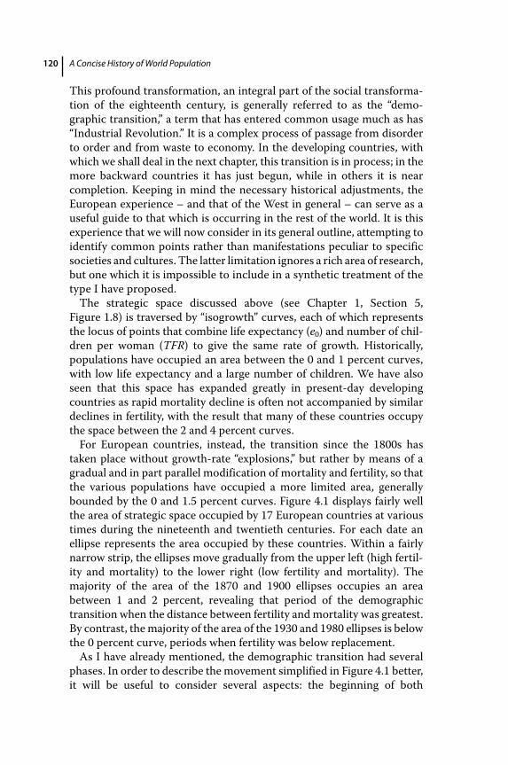
A Concise History of World Population120
This profound transformation, an integral part of the social transformation of the eighteenth century, is generally referred to as the “demographic transition,” a term that has entered common usage much as has “Industrial Revolution.” It is a complex process of passage from disorder to order and from waste to economy. In the developing countries, with which we shall deal in the next chapter, this transition is in process; in the more backward countries it has just begun, while in others it is near c ompletion. Keeping in mind the necessary historical adjustments, the European experience – and that of the West in general – can serve as a useful guide to that which is occurring in the rest of the world. It is this experience that we will now consider in its general outline, attempting to identify common points rather than manifestations peculiar to specific societies and cultures. The latter limitation ignores a rich area of research, but one which it is impossible to include in a synthetic treatment of the type I have proposed.
The strategic space discussed above (see Chapter 1, Section 5, Figure 1.8) is traversed by “isogrowth” curves, each of which represents the locus of points that combine life expectancy (e0) and number of children per woman (TFR) to give the same rate of growth. Historically, populations have occupied an area between the 0 and 1 percent curves, with low life expectancy and a large number of children. We have also seen that this space has expanded greatly in present‐day developing countries as rapid mortality decline is often not accompanied by similar declines in fertility, with the result that many of these countries occupy the space between the 2 and 4 percent curves.
For European countries, instead, the transition since the 1800s has taken place without growth‐rate “explosions,” but rather by means of a gradual and in part parallel modification of mortality and fertility, so that the various populations have occupied a more limited area, generally bounded by the 0 and 1.5 percent curves. Figure 4.1 displays fairly well the area of strategic space occupied by 17 European countries at various times during the nineteenth and twentieth centuries. For each date an ellipse represents the area occupied by these countries. Within a fairly narrow strip, the ellipses move gradually from the upper left (high fertility and mortality) to the lower right (low fertility and mortality). The majority of the area of the 1870 and 1900 ellipses occupies an area between 1 and 2 percent, revealing that period of the demographic t ransition when the distance between fertility and mortality was greatest. By contrast, the majority of the area of the 1930 and 1980 ellipses is below the 0 percent curve, periods when fertility was below replacement.
As I have already mentioned, the demographic transition had several phases. In order to describe the movement simplified in Figure 4.1 better, it will be useful to consider several aspects: the beginning of both
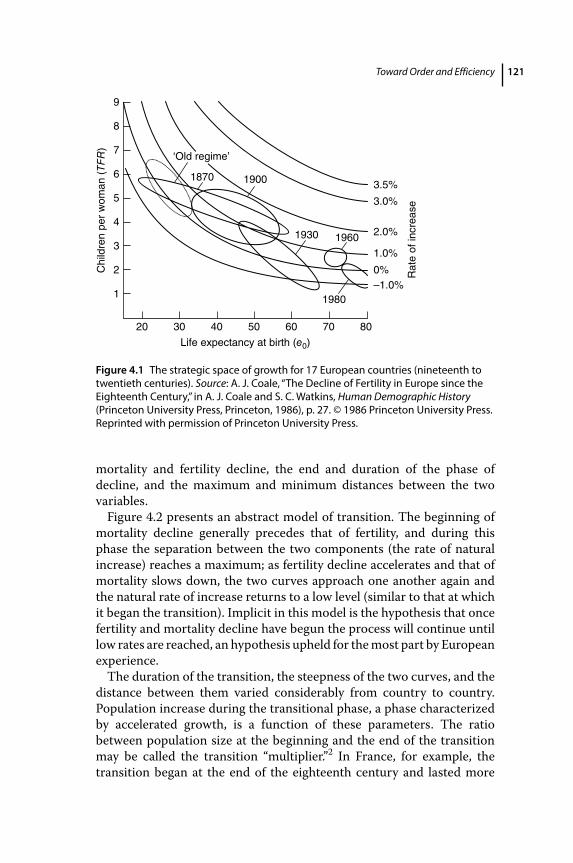
Toward Order and Efficiency 121
mortality and fertility decline, the end and duration of the phase of decline, and the maximum and minimum distances between the two variables.
Figure 4.2 presents an abstract model of transition. The beginning of mortality decline generally precedes that of fertility, and during this phase the separation between the two components (the rate of natural increase) reaches a maximum; as fertility decline accelerates and that of mortality slows down, the two curves approach one another again and the natural rate of increase returns to a low level (similar to that at which it began the transition). Implicit in this model is the hypothesis that once fertility and mortality decline have begun the process will continue until low rates are reached, an hypothesis upheld for the most part by European experience.
The duration of the transition, the steepness of the two curves, and the distance between them varied considerably from country to country. Population increase during the transitional phase, a phase characterized by accelerated growth, is a function of these parameters. The ratio between population size at the beginning and the end of the transition may be called the transition “multiplier.”2 In France, for example, the transition began at the end of the eighteenth century and lasted more
20
1
2
3
4
Chi
ldre
n pe
r w
oman
(TF
R)
5
1870 1900
1930 1960
1980
6
7
8
9
30 40 50
Life expectancy at birth (e0)
60 70 80
–1.0%0%
1.0%
2.0%
3.0%
Rat
e of
incr
ease
3.5%
‘Old regime’
Figure 4.1 The strategic space of growth for 17 European countries (nineteenth to twentieth centuries). Source: A. J. Coale, “The Decline of Fertility in Europe since the Eighteenth Century,” in A. J. Coale and S. C. Watkins, Human Demographic History (Princeton University Press, Princeton, 1986), p. 27. © 1986 Princeton University Press. Reprinted with permission of Princeton University Press.
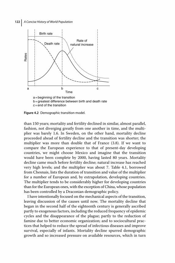
A Concise History of World Population122
than 150 years; mortality and fertility declined in similar, almost parallel, fashion, not diverging greatly from one another in time, and the multiplier was barely 1.6. In Sweden, on the other hand, mortality decline proceeded ahead of fertility decline and the transition was shorter; the multiplier was more than double that of France (3.8). If we want to c ompare the European experience to that of present‐day developing countries, we might choose Mexico and imagine that the transition would have been complete by 2000, having lasted 80 years. Mortality decline came much before fertility decline; natural increase has reached very high levels; and the multiplier was about 7. Table 4.1, borrowed from Chesnais, lists the duration of transition and value of the multiplier for a number of European and, by extrapolation, developing countries. The multiplier tends to be considerably higher for developing countries than for the European ones, with the exception of China, whose population has been controlled by a Draconian demographic policy.
I have intentionally focused on the mechanical aspects of the transition, leaving discussion of the causes until now. The mortality decline that began in the second half of the eighteenth century is generally ascribed partly to exogenous factors, including the reduced frequency of epidemic cycles and the disappearance of the plague; partly to the reduction of famine due to better economic organization; and to sociocultural practices that helped to reduce the spread of infectious diseases and improve survival, especially of infants. Mortality decline spurred demographic growth and so increased pressure on available resources, which in turn
Birth rate
Death rate
Time
a = beginning of the transitionb = greatest difference between birth and death ratec = end of the transition
b ca
Rate ofnatural increase
Rat
es
Figure 4.2 Demographic transition model.
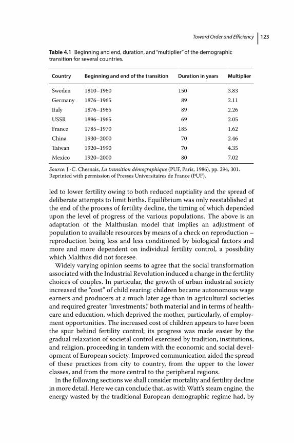
Toward Order and Efficiency 123
led to lower fertility owing to both reduced nuptiality and the spread of deliberate attempts to limit births. Equilibrium was only reestablished at the end of the process of fertility decline, the timing of which depended upon the level of progress of the various populations. The above is an adaptation of the Malthusian model that implies an adjustment of p opulation to available resources by means of a check on reproduction – reproduction being less and less conditioned by biological factors and more and more dependent on individual fertility control, a possibility which Malthus did not foresee.
Widely varying opinion seems to agree that the social transformation associated with the Industrial Revolution induced a change in the fertility choices of couples. In particular, the growth of urban industrial society increased the “cost” of child rearing: children became autonomous wage earners and producers at a much later age than in agricultural societies and required greater “investments,” both material and in terms of healthcare and education, which deprived the mother, particularly, of employment opportunities. The increased cost of children appears to have been the spur behind fertility control; its progress was made easier by the gradual relaxation of societal control exercised by tradition, institutions, and religion, proceeding in tandem with the economic and social development of European society. Improved communication aided the spread of these practices from city to country, from the upper to the lower classes, and from the more central to the peripheral regions.
In the following sections we shall consider mortality and fertility decline in more detail. Here we can conclude that, as with Watt’s steam engine, the energy wasted by the traditional European demographic regime had, by
Table 4.1 Beginning and end, duration, and “multiplier” of the demographic transition for several countries.
Country Beginning and end of the transition Duration in years Multiplier
Sweden 1810–1960 150 3.83Germany 1876–1965 89 2.11Italy 1876–1965 89 2.26USSR 1896–1965 69 2.05France 1785–1970 185 1.62China 1930–2000 70 2.46Taiwan 1920–1990 70 4.35Mexico 1920–2000 80 7.02
Source: J.‐C. Chesnais, La transition démographique (PUF, Paris, 1986), pp. 294, 301. Reprinted with permission of Presses Universitaires de France (PUF).
A Concise History of World Population124
the second half of the twentieth century, been enormously reduced. In the contemporary “economic” regime, a small number of births are sufficient to compensate for a small number of deaths; and yet, at the beginning of the third millennium, these societies seem no longer inclined to produce even those few births that would maintain d emographic equilibrium.
4.2 From Disorder to Order: The Lengthening of Life
In the second half of the eighteenth century mortality began to show signs of decline: life lengthened and the hierarchical sequence of death, dictated by age, became firmly rooted. Out of the disorder of earlier times, owing to random and unpredictable mortality, the processes of life became orderly. Two connected factors essentially explain the earlier capricious nature of death. The first was the frequent and irregular occurrence of mortality crises which, stemming from a variety of causes, slashed away sectors of all ages and classes, seriously upsetting the life of a society. Leaving aside the catastrophes brought about by the plague (the 1630 plague wiped out almost half of the population of Milan; that of 1656 half that of Genoa and Naples3), a doubling of the already high number of annual deaths (a frequent enough occurrence) was a traumatic experience for the social body. The second factor was the risk that the natural age‐linked and chronological succession of death would be overturned. Ignoring infant mortality – so frequent as to be considered almost normal – the probability that young or adolescent children would die before their parents was high. If we take, for example, French mortality in the mid‐eighteenth century (expectation of life at birth was between 25 and 28 years in the period 1740–90), then we can estimate that the probability that a 40‐year‐old mother would outlive her 10‐year‐old son over the course of the following 20 years was one in four. With today’s low mortality, this same probability is almost insignificant.4
If I have emphasized the importance of the introduction of order and regularity – I shall discuss the lengthening of life later – it is because these are essential prerequisites for development: “Perhaps only a society freed from the fear as well as from the material and spiritual consequences of sudden death was able to achieve that high rate of intellectual and technical progress without which population growth could not have been sustained.”5
The decline in the intensity and frequency of mortality crises, of those sudden and short‐term – from a few weeks to a couple of years in the case of a serious epidemic – increases of the normal death rate, constitutes the first aspect of the mortality transition. A wide range of events come under
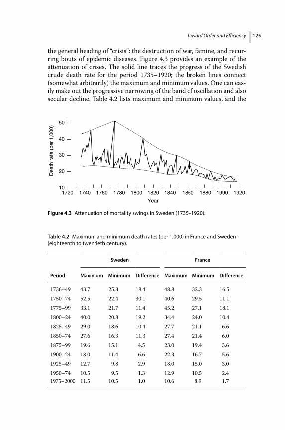
Toward Order and Efficiency 125
the general heading of “crisis”: the destruction of war, famine, and recurring bouts of epidemic diseases. Figure 4.3 provides an example of the attenuation of crises. The solid line traces the progress of the Swedish crude death rate for the period 1735–1920; the broken lines connect (somewhat arbitrarily) the maximum and minimum values. One can easily make out the progressive narrowing of the band of oscillation and also secular decline. Table 4.2 lists maximum and minimum values, and the
101720 1740 1760 1780 1800 1820
Year
1840 1860 1880 1990 1920
20
30
Dea
th r
ate
(per
1,0
00)
40
50
Figure 4.3 Attenuation of mortality swings in Sweden (1735–1920).
Table 4.2 Maximum and minimum death rates (per 1,000) in France and Sweden (eighteenth to twentieth century).
Sweden France
Period Maximum Minimum Difference Maximum Minimum Difference
1736–49 43.7 25.3 18.4 48.8 32.3 16.51750–74 52.5 22.4 30.1 40.6 29.5 11.11775–99 33.1 21.7 11.4 45.2 27.1 18.11800–24 40.0 20.8 19.2 34.4 24.0 10.41825–49 29.0 18.6 10.4 27.7 21.1 6.61850–74 27.6 16.3 11.3 27.4 21.4 6.01875–99 19.6 15.1 4.5 23.0 19.4 3.61900–24 18.0 11.4 6.6 22.3 16.7 5.61925–49 12.7 9.8 2.9 18.0 15.0 3.01950–741975–2000
10.511.5
9.510.5
1.31.0
12.910.6
10.58.9
2.41.7
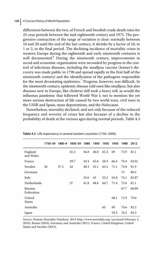
A Concise History of World Population126
differences between the two, of French and Swedish crude death rates for 25‐year periods between the mid‐eighteenth century and 1975. The progressive contraction of the range of variation is clear: normally between 10 and 20 until the end of the last century, it shrinks by a factor of 10, to 1 or 2, in the final period. The declining incidence of mortality crises in western Europe during the eighteenth and early nineteenth centuries is well documented.6 During the nineteenth century, improvements in social and economic organization were seconded by progress in the control of infectious diseases, including the smallpox vaccine (Jenner’s discovery was made public in 1798 and spread rapidly in the first half of the nineteenth century) and the identification of the pathogens responsible for the most devastating epidemics.7 Progress, however, was difficult. In the nineteenth century, epidemic disease (old ones like smallpox, but also diseases new to Europe, like cholera) still took a heavy toll, as would the influenza pandemic that followed World War I; not to mention the yet more serious destruction of life caused by two world wars, civil wars in the USSR and Spain, mass deportations, and the Holocaust.
Nonetheless, mortality declined, and not only because of the reduced frequency and severity of crises but also because of a decline in the probability of death at the various ages during normal periods. Table 4.3
Table 4.3 Life expectancy in several western countries (1750–2009).
1750–59 1800–9 1850–59 1880 1900 1930 1950 1980 2012
England and Wales
41.2 44.8 46.8 61.4 69 73.9 81.1
France 39.7 43.4 45.8 56.9 66.4 74.4 82.01Sweden 36 37.2 42 48.3 52.1 63.2 71.1 75.8 81.9Germany 73 80.5Italy 33.6 43 55.2 65.8 74.1 82.87Netherlands 37 41.8 48.8 64.7 71.4 75.8 81.1Russian Federation
67.7 68.89
United States
68.1 73.9 79.0
Australia 65 69 74.6 82.2Japan 59.3 76.2 83.3
Source: Human Mortality Database, 2012 http://www.mortality.org/ [accessed February 3, 2016]: Russia (2010), Germany and Australia (2011), France, United Kingdom, United States and Sweden (2013).
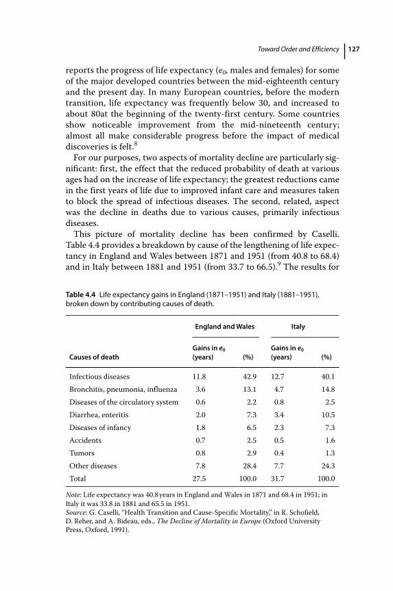
Toward Order and Efficiency 127
reports the progress of life expectancy (e0, males and females) for some of the major developed countries between the mid‐eighteenth century and the present day. In many European countries, before the modern transition, life expectancy was frequently below 30, and increased to about 80at the beginning of the twenty‐first century. Some countries show noticeable improvement from the mid‐nineteenth century; almost all make considerable progress before the impact of medical discoveries is felt.8
For our purposes, two aspects of mortality decline are particularly significant: first, the effect that the reduced probability of death at various ages had on the increase of life expectancy; the greatest reductions came in the first years of life due to improved infant care and measures taken to block the spread of infectious diseases. The second, related, aspect was the decline in deaths due to various causes, primarily infectious diseases.
This picture of mortality decline has been confirmed by Caselli. Table 4.4 provides a breakdown by cause of the lengthening of life expectancy in England and Wales between 1871 and 1951 (from 40.8 to 68.4) and in Italy between 1881 and 1951 (from 33.7 to 66.5).9 The results for
Table 4.4 Life expectancy gains in England (1871–1951) and Italy (1881–1951), broken down by contributing causes of death.
Causes of death
England and Wales Italy
Gains in e0
(years) (%)Gains in e0
(years) (%)
Infectious diseases 11.8 42.9 12.7 40.1Bronchitis, pneumonia, influenza 3.6 13.1 4.7 14.8Diseases of the circulatory system 0.6 2.2 0.8 2.5Diarrhea, enteritis 2.0 7.3 3.4 10.5Diseases of infancy 1.8 6.5 2.3 7.3Accidents 0.7 2.5 0.5 1.6Tumors 0.8 2.9 0.4 1.3Other diseases 7.8 28.4 7.7 24.3Total 27.5 100.0 31.7 100.0
Note: Life expectancy was 40.8 years in England and Wales in 1871 and 68.4 in 1951; in Italy it was 33.8 in 1881 and 65.5 in 1951.Source: G. Caselli, “Health Transition and Cause‐Specific Mortality,” in R. Schofield, D. Reher, and A. Bideau, eds., The Decline of Mortality in Europe (Oxford University Press, Oxford, 1991).
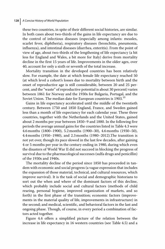
A Concise History of World Population128
these two countries, in spite of their different social histories, are similar. In both cases about two‐thirds of the gains in life expectancy are due to the control of infectious diseases (especially among infants: measles, scarlet fever, diphtheria), respiratory diseases (bronchitis, pneumonia, influenza), and intestinal diseases (diarrhea, enteritis). From the point of view of age, about two‐thirds of the lengthening of life expectancy (a bit less for England and Wales, a bit more for Italy) derive from mortality decline in the first 15 years of life. Improvements in the older ages, over 40, account for only a sixth or seventh of the total increase.
Mortality transition in the developed countries has been relatively slow. For example, the date at which female life expectancy reached 50 (at which level a cohort’s losses due to mortality between birth and the onset of reproductive age is still considerable, between 20 and 25 percent, and the “waste” of reproductive potential is about 30 percent) varies between 1861 for Norway and the 1930s for Bulgaria, Portugal, and the Soviet Union. The median date for European countries is 1903.10
Gains in life expectancy accelerated until the middle of the twentieth century. Between 1750 and 1850 England, France, and Sweden gained less than a month of life expectancy for each calendar year. These three countries, together with the Netherlands and the United States, gained about 2 months per year between 1850–9 and 1880. In the following five periods the average annual gains for the countries listed in Table 4.3 were 4.6 months (1800–1900), 5.2 months (1900–30), 4.6 months (1930–50), 4.4 months (1950–1980), and 2.3 months (1980–2012).The transition is not yet over, though its pace slowed in the last few decades, after gaining 4 or 5 months per year in the century ending in 1980, during which even the disasters of World War II did not succeed in blocking the progress of survival due to the pharmacological successes (sulfa drugs and penicillin) of the 1930s and 1940s.
The mortality decline of the period since 1850 has proceeded in tandem with economic and social progress (a vague expression that includes the expansion of those material, technical, and cultural resources, which improve survival). It is the task of social and demographic historians to sort out the when and where of the dominant factors of this decline, which probably include social and cultural factors (methods of child rearing, personal hygiene, improved organization of markets, and so forth) in the first phase of the transition; economic factors (improvements in the material quality of life, improvements in infrastructure) in the second; and medical, scientific, and behavioral factors in the last and ongoing phase. Though, of course, in every period a combination of factors acted together.
Figure 4.4 offers a simplified picture of the relation between the increase in life expectancy in 16 western countries (see Table 4.5) and a
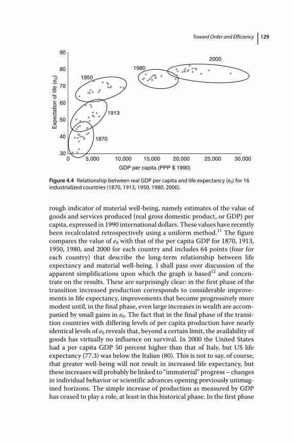
Toward Order and Efficiency 129
rough indicator of material well‐being, namely estimates of the value of goods and services produced (real gross domestic product, or GDP) per capita, expressed in 1990 international dollars. These values have recently been recalculated retrospectively using a uniform method.11 The figure compares the value of e0 with that of the per capita GDP for 1870, 1913, 1950, 1980, and 2000 for each country and includes 64 points (four for each country) that describe the long‐term relationship between life expectancy and material well‐being. I shall pass over discussion of the apparent simplifications upon which the graph is based12 and concentrate on the results. These are surprisingly clear: in the first phase of the transition increased production corresponds to considerable improvements in life expectancy, improvements that become progressively more modest until, in the final phase, even large increases in wealth are accompanied by small gains in e0. The fact that in the final phase of the transition countries with differing levels of per capita production have nearly identical levels of e0 reveals that, beyond a certain limit, the availability of goods has virtually no influence on survival. In 2000 the United States had a per capita GDP 50 percent higher than that of Italy, but US life expectancy (77.3) was below the Italian (80). This is not to say, of course, that greater well‐being will not result in increased life expectancy, but these increases will probably be linked to “immaterial” progress – changes in individual behavior or scientific advances opening previously unimagined horizons. The simple increase of production as measured by GDP has ceased to play a role, at least in this historical phase. In the first phase
300 5,000 10,000
1870
1913
1950
1980
2000
15,000
GDP per capita (PPP $ 1990)
20,000 25,000 30,000
40
50
60
70
Exp
ecta
tion
of li
fe (
e 0)
80
90
Figure 4.4 Relationship between real GDP per capita and life expectancy (e0) for 16 industrialized countries (1870, 1913, 1950, 1980, 2000).
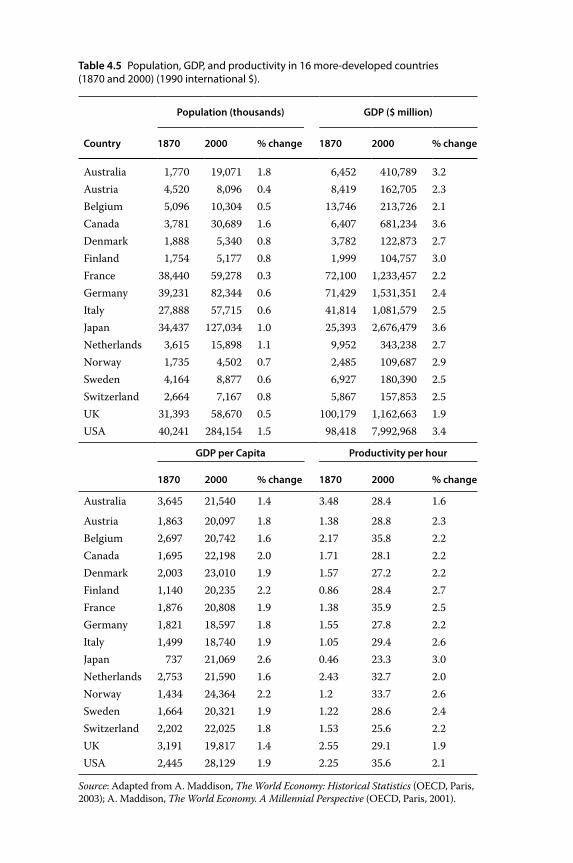
Table 4.5 Population, GDP, and productivity in 16 more‐developed countries (1870 and 2000) (1990 international $).
Population (thousands) GDP ($ million)
Country 1870 2000 % change 1870 2000 % change
Australia 1,770 19,071 1.8 6,452 410,789 3.2Austria 4,520 8,096 0.4 8,419 162,705 2.3Belgium 5,096 10,304 0.5 13,746 213,726 2.1Canada 3,781 30,689 1.6 6,407 681,234 3.6Denmark 1,888 5,340 0.8 3,782 122,873 2.7Finland 1,754 5,177 0.8 1,999 104,757 3.0France 38,440 59,278 0.3 72,100 1,233,457 2.2Germany 39,231 82,344 0.6 71,429 1,531,351 2.4Italy 27,888 57,715 0.6 41,814 1,081,579 2.5Japan 34,437 127,034 1.0 25,393 2,676,479 3.6Netherlands 3,615 15,898 1.1 9,952 343,238 2.7Norway 1,735 4,502 0.7 2,485 109,687 2.9Sweden 4,164 8,877 0.6 6,927 180,390 2.5Switzerland 2,664 7,167 0.8 5,867 157,853 2.5UK 31,393 58,670 0.5 100,179 1,162,663 1.9USA 40,241 284,154 1.5 98,418 7,992,968 3.4
GDP per Capita Productivity per hour
1870 2000 % change 1870 2000 % change
Australia 3,645 21,540 1.4 3.48 28.4 1.6
Austria 1,863 20,097 1.8 1.38 28.8 2.3Belgium 2,697 20,742 1.6 2.17 35.8 2.2Canada 1,695 22,198 2.0 1.71 28.1 2.2Denmark 2,003 23,010 1.9 1.57 27.2 2.2Finland 1,140 20,235 2.2 0.86 28.4 2.7France 1,876 20,808 1.9 1.38 35.9 2.5Germany 1,821 18,597 1.8 1.55 27.8 2.2Italy 1,499 18,740 1.9 1.05 29.4 2.6Japan 737 21,069 2.6 0.46 23.3 3.0Netherlands 2,753 21,590 1.6 2.43 32.7 2.0Norway 1,434 24,364 2.2 1.2 33.7 2.6Sweden 1,664 20,321 1.9 1.22 28.6 2.4Switzerland 2,202 22,025 1.8 1.53 25.6 2.2UK 3,191 19,817 1.4 2.55 29.1 1.9USA 2,445 28,129 1.9 2.25 35.6 2.1
Source: Adapted from A. Maddison, The World Economy: Historical Statistics (OECD, Paris, 2003); A. Maddison, The World Economy. A Millennial Perspective (OECD, Paris, 2001).
Toward Order and Efficiency 131
of the transition increased production translated into greatly improved survival, for obvious reasons: more food, better clothing, better houses, and more medical care have a notable effect on those who are malnourished, badly clothed, poorly housed, and forced to trust fate in case of sickness. On the other hand, when increased production benefits already prosperous populations the effects are minimal or nonexistent, if not negative, as may be the case with overeating and environmental deterioration.
4.3 From High to Low Fertility
Fertility decline, like that of mortality, was a gradual and geographically varied process. I have already discussed the combination of factors, both biological (which determine birth intervals) and social (which determine the portion of the reproductive period devoted to childbearing: age at marriage, proportion marrying), which regulate the “production” of c hildren (see Chapter 1, Section 4).13 As we have seen, these factors were able to significantly influence fertility, so that prior to the transition European levels ranged from a low of about 30 per 1,000 to a high of above 45. Nonetheless, voluntary fertility control14 was the decisive f actor in fertility decline – certainly a more efficient method than extended breast‐feeding, late marriage, or remaining single.
Figure 4.5 records the effectiveness of the marital check in Europe during the period leading up to the fertility decline. Low‐nuptiality female populations occupy the upper left portion of the graph: they are characterized by a high age at first marriage (over 27 in Switzerland, Belgium, Sweden, and Norway) and a low proportion of women who have married before the end of the reproductive period (a little over 80 percent). In the lower right of the graph are high‐nuptiality populations (Romania, Bulgaria), with low age at first marriage (around 20) and a high percentage married (over 95 percent). In the premodern age there existed a fairly strong (and inverse) relationship between the two components of nuptiality, as revealed by the graph.
Figure 4.5 gives an idea of the variability of pretransition nuptiality and, indirectly, the degree to which it controlled the production of births. And while the level of control was considerable, it was not sufficient to regulate fertility during the rapid social transformation of the previous century; more efficient control was provided by voluntary fertility limitation. Birth control, for a time virtually unknown except to select groups (nobility, the urban bourgeoisie),15 appeared in France and a few restricted areas toward the end of the eighteenth century16 and spread rapidly throughout Europe during the second half of the nineteenth – though
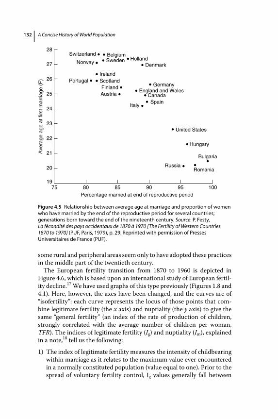
A Concise History of World Population132
some rural and peripheral areas seem only to have adopted these p ractices in the middle part of the twentieth century.
The European fertility transition from 1870 to 1960 is depicted in Figure 4.6, which is based upon an international study of European fertility decline.17 We have used graphs of this type previously (Figures 1.8 and 4.1). Here, however, the axes have been changed, and the curves are of “isofertility”: each curve represents the locus of those points that combine legitimate fertility (the x axis) and nuptiality (the y axis) to give the same “general fertility” (an index of the rate of production of children, strongly correlated with the average number of children per woman, TFR). The indices of legitimate fertility (Ig) and nuptiality (Im), explained in a note,18 tell us the following:
1) The index of legitimate fertility measures the intensity of childbearing within marriage as it relates to the maximum value ever encountered in a normally constituted population (value equal to one). Prior to the spread of voluntary fertility control, Ig values generally fall between
Switzerland BelgiumSweden Holland
Denmark
GermanyEngland and Wales
CanadaSpain
Italy
IrelandScotlandFinlandAustria
Portugal
Norway
United States
Hungary
Bulgaria
Russia
7519
20
21
22
23
24
25
Ave
rage
age
at f
irst m
arria
ge (
F) 26
27
28
80 85 90 95 100
Romania
Percentage married at end of reproductive period
Figure 4.5 Relationship between average age at marriage and proportion of women who have married by the end of the reproductive period for several countries; generations born toward the end of the nineteenth century. Source: P. Festy, La fécondité des pays occidentaux de 1870 à 1970 [The Fertility of Western Countries 1870 to 1970] (PUF, Paris, 1979), p. 29. Reprinted with permission of Presses Universitaires de France (PUF).
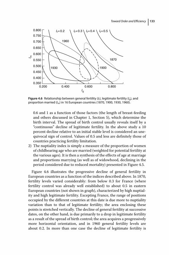
Toward Order and Efficiency 133
0.6 and 1 as a function of those factors (the length of breast‐feeding and others discussed in Chapter 1, Section 5), which determine the birth interval. The spread of birth control usually reveals itself by a “continuous” decline of legitimate fertility. In the above study a 10 percent decline relative to an initial stable level is considered an unequivocal sign of control. Values of 0.5 and less are definitely those of countries practicing fertility limitation.
2) The nuptiality index is simply a measure of the proportion of women of childbearing age who are married (weighted for potential fertility at the various ages). It is then a synthesis of the effects of age at marriage and proportions marrying (as well as of widowhood, declining in the period considered due to reduced mortality) presented in Figure 4.5.
Figure 4.6 illustrates the progressive decline of general fertility in European countries as a function of the indices described above. In 1870, fertility levels varied considerably: from below 0.3 for France (where f ertility control was already well established) to about 0.5 in eastern European countries (not shown in graph), characterized by high nuptiality and high legitimate fertility. Excepting France, the range of positions occupied by the different countries at this date is due more to nuptiality variation than to that of legitimate fertility; the area enclosing these points is stretched vertically. The decline of general fertility at successive dates, on the other hand, is due primarily to a drop in legitimate fertility as a result of the spread of birth control; the area acquires a progressively more horizontal orientation, and in 1960 general fertility levels are about 0.2. In more than one case the decline of legitimate fertility is
0.2000.350
0.400
0.450
0.500
0.550
0.600
0.650
0.700
0.750
0.800
0.400
1930
1960
1870
If= 0.2 If= 0.3
Ig
I mIf= 0.4 If= 0.5
1900
0.600 0.800
Figure 4.6 Relationship between general fertility (If), legitimate fertility (Ig), and proportion married (Im) in 16 European countries (1870, 1900, 1930, 1960).
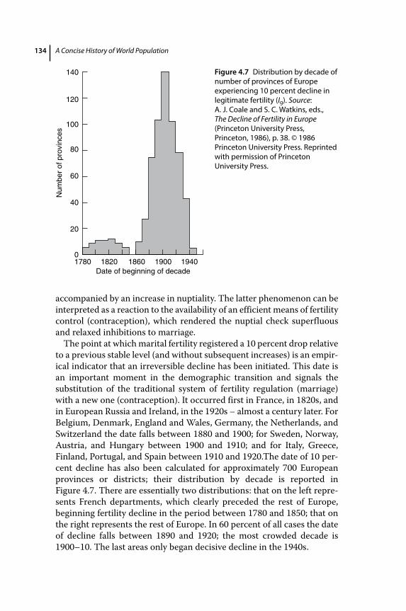
A Concise History of World Population134
accompanied by an increase in nuptiality. The latter phenomenon can be interpreted as a reaction to the availability of an efficient means of fertility control (contraception), which rendered the nuptial check superfluous and relaxed inhibitions to marriage.
The point at which marital fertility registered a 10 percent drop relative to a previous stable level (and without subsequent increases) is an empirical indicator that an irreversible decline has been initiated. This date is an important moment in the demographic transition and signals the substitution of the traditional system of fertility regulation (marriage) with a new one (contraception). It occurred first in France, in 1820s, and in European Russia and Ireland, in the 1920s – almost a century later. For Belgium, Denmark, England and Wales, Germany, the Netherlands, and Switzerland the date falls between 1880 and 1900; for Sweden, Norway, Austria, and Hungary between 1900 and 1910; and for Italy, Greece, Finland, Portugal, and Spain between 1910 and 1920.The date of 10 percent decline has also been calculated for approximately 700 European provinces or districts; their distribution by decade is reported in Figure 4.7. There are essentially two distributions: that on the left represents French departments, which clearly preceded the rest of Europe, beginning fertility decline in the period between 1780 and 1850; that on the right represents the rest of Europe. In 60 percent of all cases the date of decline falls between 1890 and 1920; the most crowded decade is 1900–10. The last areas only began decisive decline in the 1940s.
20
01780 1820 1860
Date of beginning of decade1900 1940
40
60
Num
ber
of p
rovi
nces
80
100
120
140 Figure 4.7 Distribution by decade of number of provinces of Europe experiencing 10 percent decline in legitimate fertility (Ig). Source: A. J. Coale and S. C. Watkins, eds., The Decline of Fertility in Europe (Princeton University Press, Princeton, 1986), p. 38. © 1986 Princeton University Press. Reprinted with permission of Princeton University Press.
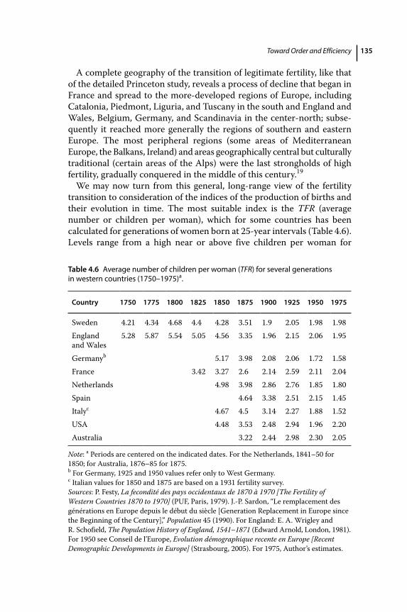
Toward Order and Efficiency 135
A complete geography of the transition of legitimate fertility, like that of the detailed Princeton study, reveals a process of decline that began in France and spread to the more‐developed regions of Europe, including Catalonia, Piedmont, Liguria, and Tuscany in the south and England and Wales, Belgium, Germany, and Scandinavia in the center‐north; subsequently it reached more generally the regions of southern and eastern Europe. The most peripheral regions (some areas of Mediterranean Europe, the Balkans, Ireland) and areas geographically central but culturally traditional (certain areas of the Alps) were the last strongholds of high fertility, gradually conquered in the middle of this century.19
We may now turn from this general, long‐range view of the fertility transition to consideration of the indices of the production of births and their evolution in time. The most suitable index is the TFR (average n umber or children per woman), which for some countries has been c alculated for generations of women born at 25‐year intervals (Table 4.6). Levels range from a high near or above five children per woman for
Table 4.6 Average number of children per woman (TFR) for several generations in western countries (1750–1975)a.
Country 1750 1775 1800 1825 1850 1875 1900 1925 1950 1975
Sweden 4.21 4.34 4.68 4.4 4.28 3.51 1.9 2.05 1.98 1.98England and Wales
5.28 5.87 5.54 5.05 4.56 3.35 1.96 2.15 2.06 1.95
Germanyb 5.17 3.98 2.08 2.06 1.72 1.58France 3.42 3.27 2.6 2.14 2.59 2.11 2.04Netherlands 4.98 3.98 2.86 2.76 1.85 1.80Spain 4.64 3.38 2.51 2.15 1.45Italyc 4.67 4.5 3.14 2.27 1.88 1.52USA 4.48 3.53 2.48 2.94 1.96 2.20Australia 3.22 2.44 2.98 2.30 2.05
Note: a Periods are centered on the indicated dates. For the Netherlands, 1841–50 for 1850; for Australia, 1876–85 for 1875.b For Germany, 1925 and 1950 values refer only to West Germany.c Italian values for 1850 and 1875 are based on a 1931 fertility survey.Sources: P. Festy, La fecondité des pays occidentaux de 1870 à 1970 [The Fertility of Western Countries 1870 to 1970] (PUF, Paris, 1979). J.‐P. Sardon, “Le remplacement des générations en Europe depuis le début du siècle [Generation Replacement in Europe since the Beginning of the Century],” Population 45 (1990). For England: E. A. Wrigley and R. Schofield, The Population History of England, 1541–1871 (Edward Arnold, London, 1981). For 1950 see Conseil de l’Europe, Evolution démographique recente en Europe [Recent Demographic Developments in Europe] (Strasbourg, 2005). For 1975, Author’s estimates.
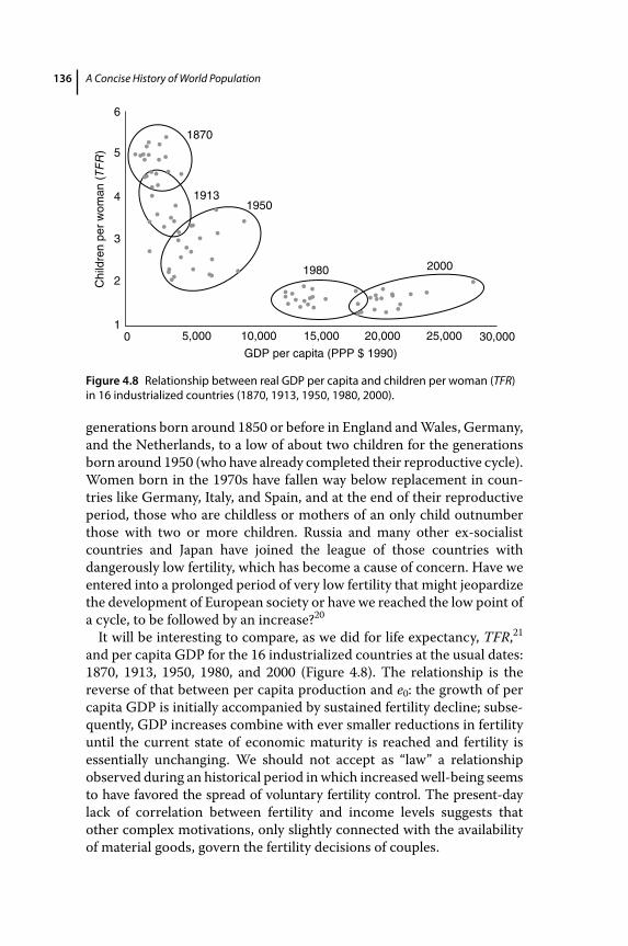
A Concise History of World Population136
g enerations born around 1850 or before in England and Wales, Germany, and the Netherlands, to a low of about two children for the generations born around 1950 (who have already completed their reproductive cycle).Women born in the 1970s have fallen way below replacement in countries like Germany, Italy, and Spain, and at the end of their reproductive period, those who are childless or mothers of an only child outnumber those with two or more children. Russia and many other ex‐socialist countries and Japan have joined the league of those countries with d angerously low fertility, which has become a cause of concern. Have we entered into a prolonged period of very low fertility that might jeopardize the development of European society or have we reached the low point of a cycle, to be followed by an increase?20
It will be interesting to compare, as we did for life expectancy, TFR,21 and per capita GDP for the 16 industrialized countries at the usual dates: 1870, 1913, 1950, 1980, and 2000 (Figure 4.8). The relationship is the reverse of that between per capita production and e0: the growth of per capita GDP is initially accompanied by sustained fertility decline; subsequently, GDP increases combine with ever smaller reductions in fertility until the current state of economic maturity is reached and fertility is essentially unchanging. We should not accept as “law” a relationship observed during an historical period in which increased well‐being seems to have favored the spread of voluntary fertility control. The present‐day lack of correlation between fertility and income levels suggests that other complex motivations, only slightly connected with the availability of material goods, govern the fertility decisions of couples.
1913
Chi
ldre
n pe
r w
oman
(TF
R)
1950
1980 2000
01
2
3
4
5
6
5,000 10,000 15,000
GDP per capita (PPP $ 1990)
20,000 25,000 30,000
1870
Figure 4.8 Relationship between real GDP per capita and children per woman (TFR) in 16 industrialized countries (1870, 1913, 1950, 1980, 2000).
Toward Order and Efficiency 137
During the nineteenth and twentieth centuries social and economic transformation was an important factor in fertility decline, confirmed by its generally slower progress in peripheral and backward areas. There have, of course, been important exceptions which, as often happens in the social sciences, have frustrated those scholars looking for simple solutions to complex problems. The following are a few examples from the many which the literature offers: (1) In rural France, fertility decline began earlier than in England, a richer and more advanced country in the midst of the Industrial Revolution. (2) In many countries the rate of fertility decline is only minimally explained by social and economic indices, such as levels of education, rurality, industrialization, or urbanization. (3) It is often the case that cultural factors – membership of a linguistic or ethnic group, religious or political affiliation – seem to be more s ignificant to fertility decline than economic factors.
But if we look at the entire process, we see that no population has maintained high levels of fertility for long in the face of increasing well‐being and declining mortality. The demographic transition has clearly been an integral part of the transformation of European society.
4.4 European Emigration: A Unique Phenomenon
The synthesis of the transition I am presenting here would not be complete without reference to the great currents of migration that populated two continents while at the same time lowering European demographic pressure. I have already discussed the importance of the availability of space (and also of land) in shaping European demographic growth prior to the Industrial Revolution. At the end of the eighteenth century, more than 8 million people of European extraction, about equally divided, inhabited the two halves of the American continent. Over three centuries Europe had by means of Iberian and British imperialism established the political, economic, and demographic foundations for the coming mass migration. The causes of that migration were both economic and demographic: economic because the Industrial Revolution and technological progress increased productivity and so rendered masses of workers superfluous, especially in rural areas; and demographic because the transition entailed a large demographic “multiplier,” which is to say it sped up population growth, and so worsened the problems created by economic changes. The availability of land and space in North and South America and to a lesser degree in Oceania, combined with the demand for labor in these new societies, created the conditions for massive migration.
A Concise History of World Population138
During the latter part of the nineteenth century and the first decades of the twentieth century, the process of economic integration between countries accelerated and extended its geographic reach. This process of globalization was due to the increased mobility of the production factors – capital, labor, and goods – and exports grew faster than production. According to Maddison, more than half the savings of Great Britain flowed abroad; other major countries, like France and Germany, also expanded their investments abroad. A great proportion of foreign investment went into the expansion of the railway networks, whose length increased fivefold in North America between 1870 and 1913 (from 90,000 to 450,000 kilometers), attracting legions of migrant workers. In Latin America, the few thousand kilometers of railways of 1870 grew to 100,000 in 1913.22 The growing economic integration is well measured by the increased ratio between the value of manufactured exports and GDP: this ratio increased from 3 percent in 1820 to 12 percent in 1870 and 18 percent in 1913 in the United Kingdom; and, between the same dates, from 1 percent to 5 percent and 8 percent in France; in Germany, from 9 percent in 1870 to 16 percent in 1913. According to O’ Rourke and Williamson, the mass migration from Europe to America that accompanied this process of globalization determined, in the countries of origin, an increase of real wages, an improved standard of living, and a reduction of poverty. However, mass migration had a relevant impact on the American labor market, where wages were moderated, and, because of the competition of the new arrivals, the standard of living of previous immigrants and of native workers declined and new poverties emerged. Mass migration, therefore, determined an economic convergence between countries, and between the standard of living of the poor countries of origin and of the wealthier countries of destination.23 Perhaps this conclusion can be reformulated by saying that, because of mass migration, the growing divergence between the standard of living of Europe and America – as measured by the income per capita (see Table 4.5) – was slowed and compressed. The following are estimates for European transoceanic migration between 1846 and 1932 from the major countries of departure: 18 million from Great Britain and Ireland, 11.1 million from Italy, 6.5 million from Spain and Portugal, 5.2 million from Austria‐Hungary, 4.9 million from Germany, 2.9 million from Poland and Russia, and 2.1 million from Sweden and Norway. This flood of emigration, which was of course b alanced to some degree by a countercurrent of return migration, went primarily to the United States (34.2 million), Argentina and Uruguay (7.1 million),Canada (5.2 million), Brazil (4.4 million), Australia and New Zealand (3.5 million), and Cuba (0.9 million). In the first 15 years of the twentieth century the annual rate of European emigration exceeded 3 per 1,000, equal to about one‐third of natural increase.24
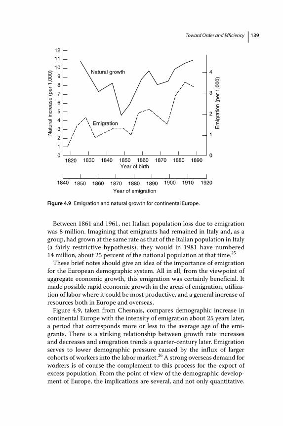
Toward Order and Efficiency 139
Between 1861 and 1961, net Italian population loss due to emigration was 8 million. Imagining that emigrants had remained in Italy and, as a group, had grown at the same rate as that of the Italian population in Italy (a fairly restrictive hypothesis), they would in 1981 have numbered 14 million, about 25 percent of the national population at that time.25
These brief notes should give an idea of the importance of emigration for the European demographic system. All in all, from the viewpoint of aggregate economic growth, this emigration was certainly beneficial. It made possible rapid economic growth in the areas of emigration, utilization of labor where it could be most productive, and a general increase of resources both in Europe and overseas.
Figure 4.9, taken from Chesnais, compares demographic increase in continental Europe with the intensity of emigration about 25 years later, a period that corresponds more or less to the average age of the emigrants. There is a striking relationship between growth rate increases and decreases and emigration trends a quarter‐century later. Emigration serves to lower demographic pressure caused by the influx of larger cohorts of workers into the labor market.26 A strong overseas demand for workers is of course the complement to this process for the export of excess population. From the point of view of the demographic development of Europe, the implications are several, and not only quantitative.
18200
1
2
3
4
0
1
2
3
4
5
6
7
8
9
10
11
12
1830 1840
1840
1850
1850
1860 1870 1880 1890
1860 1870 1880 1890
Natural growth
Emigration
Year of birth
Year of emigration
1900 1910 1920
Nat
ural
incr
ease
(pe
r 1,
000)
Em
igra
tion
(per
1,0
00)
Figure 4.9 Emigration and natural growth for continental Europe.
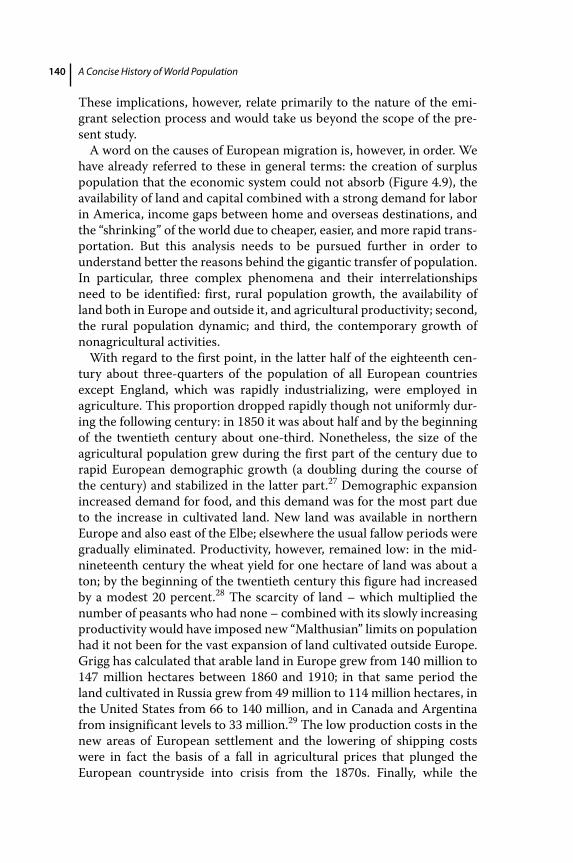
A Concise History of World Population140
These implications, however, relate primarily to the nature of the emigrant selection process and would take us beyond the scope of the present study.
A word on the causes of European migration is, however, in order. We have already referred to these in general terms: the creation of surplus population that the economic system could not absorb (Figure 4.9), the availability of land and capital combined with a strong demand for labor in America, income gaps between home and overseas destinations, and the “shrinking” of the world due to cheaper, easier, and more rapid transportation. But this analysis needs to be pursued further in order to understand better the reasons behind the gigantic transfer of population. In particular, three complex phenomena and their interrelationships need to be identified: first, rural population growth, the availability of land both in Europe and outside it, and agricultural productivity; second, the rural population dynamic; and third, the contemporary growth of nonagricultural activities.
With regard to the first point, in the latter half of the eighteenth century about three‐quarters of the population of all European countries except England, which was rapidly industrializing, were employed in agriculture. This proportion dropped rapidly though not uniformly during the following century: in 1850 it was about half and by the beginning of the twentieth century about one‐third. Nonetheless, the size of the agricultural population grew during the first part of the century due to rapid European demographic growth (a doubling during the course of the century) and stabilized in the latter part.27 Demographic expansion increased demand for food, and this demand was for the most part due to the increase in cultivated land. New land was available in northern Europe and also east of the Elbe; elsewhere the usual fallow periods were gradually eliminated. Productivity, however, remained low: in the mid‐nineteenth century the wheat yield for one hectare of land was about a ton; by the beginning of the twentieth century this figure had increased by a modest 20 percent.28 The scarcity of land – which multiplied the number of peasants who had none – combined with its slowly increasing productivity would have imposed new “Malthusian” limits on population had it not been for the vast expansion of land cultivated outside Europe. Grigg has calculated that arable land in Europe grew from 140 million to 147 million hectares between 1860 and 1910; in that same period the land cultivated in Russia grew from 49 million to 114 million hectares, in the United States from 66 to 140 million, and in Canada and Argentina from insignificant levels to 33 million.29 The low production costs in the new areas of European settlement and the lowering of shipping costs were in fact the basis of a fall in agricultural prices that plunged the European countryside into crisis from the 1870s. Finally, while the
Toward Order and Efficiency 141
productivity of land grew sluggishly, the injection of capital into the countryside and mechanization combined to increase the productivity of labor. Masses of peasants characterized by limited proprietorship and increased productivity of labor translated into a rapid increase in surplus labor, so workers frequently found themselves torn away from traditional activities and lifestyles and facing crisis situations. As a result, the pool of potential emigrants grew.30
The second point refers to the population dynamic of rural areas where birth control spread with a notable lag as compared to the cities, fostering higher rates of natural population increase during the period of the transition. In some cases – analogous to the situation in many developing countries – the first phases of the transition and the attendant improvements in sanitary conditions led to an increase rather than a decrease in fertility.31
The third point refers to the rapidity with which new nonagricultural activities sprang into existence in Europe and so provided an alternative outlet for rural population excess. This phenomenon is not of course independent of the stage of evolution of agriculture; indeed the two are intimately connected: tools, machines, and fertilizers that had previously been produced by agricultural concerns came gradually to be more efficiently created by the industrial system. But it was the growth of this latter system and of predominantly urban service activities that created new opportunities for surplus rural labor. In those areas where this process occurred relatively early, emigration was low or in any case short‐lived; by contrast, in those areas where it took place relatively late, emigration tended to be massive. The ratio between those employed in manufacturing industries and those employed in agriculture serves as an index of the changing situation (Figure 4.10). When this ratio is greater than one (that is, when those employed in manufacturing exceed those in agriculture), then the pressure to emigrate becomes weaker and eventually disappears as the modern sector of the economy – which initially consisted of the manufacturing industries but then grew to include transportation, services, building, and so on – becomes sufficiently important to absorb the remaining agricultural surplus population. The United Kingdom, from which mass emigration had long ceased, well exceeded a 1:1 ratio during the late‐nineteenth century. Prior to World War I, this ratio was surpassed by those countries undergoing a rapid process of industrialization: Belgium, where mass emigration had never taken hold, and Germany and Switzerland, where it had ceased. Mediterranean countries like Italy and Spain, where industrialization came late, only exceeded this ratio in the 1960s and 1970s, at which time large‐scale emigration came to an end. In other countries where manufacturing industries came to dominate the national economy in the period between the
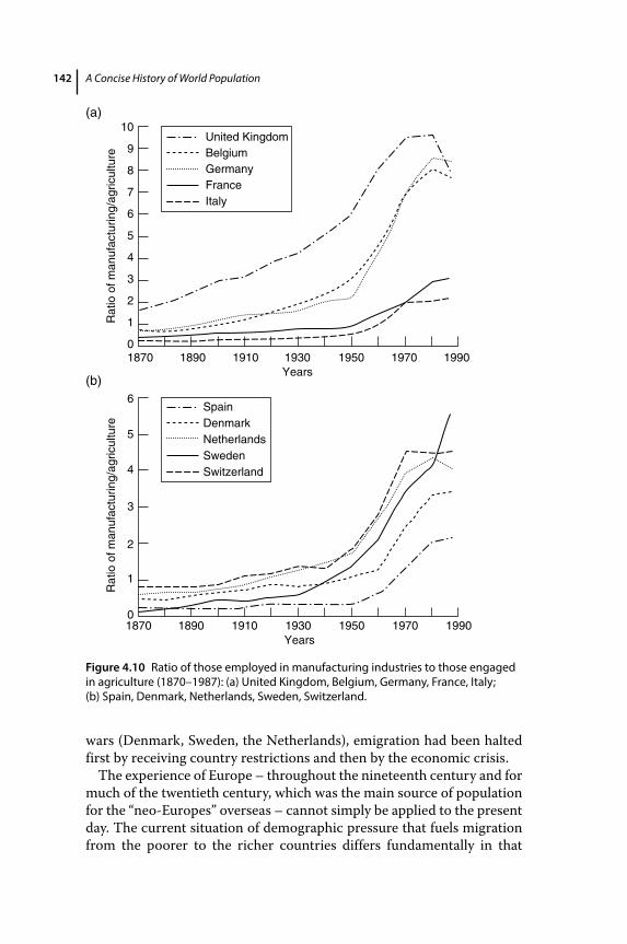
A Concise History of World Population142
wars (Denmark, Sweden, the Netherlands), emigration had been halted first by receiving country restrictions and then by the economic crisis.
The experience of Europe – throughout the nineteenth century and for much of the twentieth century, which was the main source of population for the “neo‐Europes” overseas – cannot simply be applied to the present day. The current situation of demographic pressure that fuels migration from the poorer to the richer countries differs fundamentally in that
1870 1890
United Kingdom
(a)
(b)
BelgiumGermanyFranceItaly
1910 1930Years
SpainDenmarkNetherlandsSwedenSwitzerland
1950 1970 1990
18700
1
2
3
4
5
6
0
1
2
3
4
5
Rat
io o
f man
ufac
turin
g/ag
ricul
ture
Rat
io o
f man
ufac
turin
g/ag
ricul
ture
6
7
8
10
9
1890 1910 1930Years
1950 1970 1990
Figure 4.10 Ratio of those employed in manufacturing industries to those engaged in agriculture (1870–1987): (a) United Kingdom, Belgium, Germany, France, Italy; (b) Spain, Denmark, Netherlands, Sweden, Switzerland.
Toward Order and Efficiency 143
“empty” areas open to immigration no longer exist and national policies severely limit the possibilities for human movement. On the other hand, economic globalization tends to increase inequalities between countries, creating widening income gaps between rich and poor areas and thus increasing incentives to migrate. However, globalization may also foster growth, pushing an increasing portion of developing countries’ populations to modest levels of well‐being. When these are reached, the cost of emigration – particularly its social and cultural components – tends to increase more rapidly, thus reducing the propensity to leave one’s country.
4.5 A Summing Up: The Results of the Transition
The demographic transition and associated migration left the European population profoundly changed, both dynamically and structurally. The changes associated with the achievement of a high level of demographic efficiency can be expressed by several indices. Table 4.7 lists these for Italy in 1881 and 1981, approximately the beginning and ending dates for the demographic transition in that country. With certain adaptations the Italian case is typical of Europe as a whole. The “position” of Italy in the context of the demographic transition of the 15 western countries plus Japan (see the list in Table 4.5) can be appreciated in Figure 4.11. In 1870 and in 1913 Italy is clearly a “laggard,” with higher mortality and fertility than the other countries; in 2000, on the other hand, it is in the vanguard, with lower than average fertility and higher than average expectation of life.
But let us return to Table 4.7, which requires a brief commentary. The birth and death rates repeat what we have already discussed in the previous pages, namely the reduced intensity, by about two‐thirds, of both phenomena; at the same time, life expectancy more than doubled as survivorship increased immensely. In 1981, 98 percent of each generation arrived at reproductive age (15 years) and 42 percent achieved the respectable age of 80. At 1881 these figures were 58 and 6 percent. Clearly these dramatic improvements make important changes to a society.32
The measures of nuptiality and family structure provide a less clear picture, revealing both stability and change at the same time. Age at m arriage and the proportion of women remaining single at the end of the reproductive period were stable, confirmation that in the West the n uptial check played a minimal role in the dramatic changes that took place. While fertility declined, utilization of the reproductive space decreased considerably, as revealed by the decrease in average ages at
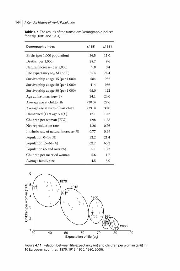
A Concise History of World Population144
Table 4.7 The results of the transition: Demographic indices for Italy (1881 and 1981).
Demographic index c.1881 c.1981
Births (per 1,000 population) 36.5 11.0Deaths (per 1,000) 28.7 9.6Natural increase (per 1,000) 7.8 0.4Life expectancy (e0, M and F) 35.4 74.4Survivorship at age 15 (per 1,000) 584 982Survivorship at age 50 (per 1,000) 414 936Survivorship at age 80 (per 1,000) 65.0 422Age at first marriage (F) 24.1 24.0Average age at childbirth (30.0) 27.6Average age at birth of last child (39.0) 30.0Unmarried (F) at age 50 (%) 12.1 10.2Children per woman (TFR) 4.98 1.58Net reproduction rate 1.26 0.76Intrinsic rate of natural increase (%) 0.77 0.99Population 0–14 (%) 32.2 21.4Population 15–64 (%) 62.7 65.3Population 65 and over (%) 5.1 13.3Children per married woman 5.6 1.7Average family size 4.5 3.0
301
2
3
4
Chi
ldre
n pe
r w
oman
(TF
R)
5
6
40 50 60Expectation of life (e0)
70 80 90
2000
1980
1950
1913
1870
IT
IT
IT
IT
IT
Figure 4.11 Relation between life expectancy (e0) and children per woman (TFR) in 16 European countries (1870, 1913, 1950, 1980, 2000).
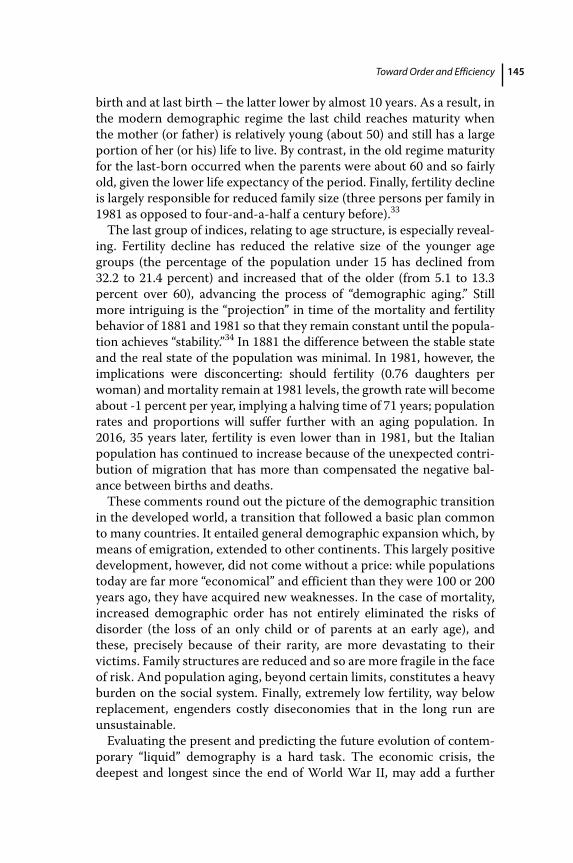
Toward Order and Efficiency 145
birth and at last birth – the latter lower by almost 10 years. As a result, in the modern demographic regime the last child reaches maturity when the mother (or father) is relatively young (about 50) and still has a large portion of her (or his) life to live. By contrast, in the old regime maturity for the last‐born occurred when the parents were about 60 and so fairly old, given the lower life expectancy of the period. Finally, fertility decline is largely responsible for reduced family size (three persons per family in 1981 as opposed to four‐and‐a‐half a century before).33
The last group of indices, relating to age structure, is especially revealing. Fertility decline has reduced the relative size of the younger age groups (the percentage of the population under 15 has declined from 32.2 to 21.4 percent) and increased that of the older (from 5.1 to 13.3 percent over 60), advancing the process of “demographic aging.” Still more intriguing is the “projection” in time of the mortality and fertility behavior of 1881 and 1981 so that they remain constant until the population achieves “stability.”34 In 1881 the difference between the stable state and the real state of the population was minimal. In 1981, however, the implications were disconcerting: should fertility (0.76 daughters per woman) and mortality remain at 1981 levels, the growth rate will become about ‐1 percent per year, implying a halving time of 71 years; population rates and proportions will suffer further with an aging population. In 2016, 35 years later, fertility is even lower than in 1981, but the Italian population has continued to increase because of the unexpected contribution of migration that has more than compensated the negative balance between births and deaths.
These comments round out the picture of the demographic transition in the developed world, a transition that followed a basic plan common to many countries. It entailed general demographic expansion which, by means of emigration, extended to other continents. This largely positive development, however, did not come without a price: while populations today are far more “economical” and efficient than they were 100 or 200 years ago, they have acquired new weaknesses. In the case of mortality, increased demographic order has not entirely eliminated the risks of disorder (the loss of an only child or of parents at an early age), and these, precisely because of their rarity, are more devastating to their v ictims. Family structures are reduced and so are more fragile in the face of risk. And population aging, beyond certain limits, constitutes a heavy burden on the social system. Finally, extremely low fertility, way below replacement, engenders costly diseconomies that in the long run are unsustainable.
Evaluating the present and predicting the future evolution of contemporary “liquid” demography is a hard task. The economic crisis, the deepest and longest since the end of World War II, may add a further
A Concise History of World Population146
discontinuity from the past. In 2016, most European countries approach an expectation of life of 85 years; fertility, with minor fluctuations, hovers around 1.6 children per woman; the population in adult and active ages is shrinking; women reaching their 70th birthday are as numerous as girls reaching puberty; the inflow of refugees has dwarfed the traditional forms of migration.
4.6 Theoretical Considerations on the Relationship between Demographic and Economic Growth
The advent of the Industrial Revolution, the introduction of machinery, the exploitation of new sources of energy, and increased trade all combined to rapidly alter the terms of the population/land/labor equation. Population growth no longer led, by means of increased demand, to a rise in prices and a decline in wages. Beginning in the nineteenth century, European population, in spite of considerable growing pains, nonetheless grew in a climate of declining prices and increasing wages. The difficult balance between population and land was broken as economic and demographic growth became not competing but complementary forces. This, however, is only a general picture; clearly the attempt to describe more specifically the nature of the relationship between population and economy is a difficult undertaking. One is inclined to adopt Schumpeter’s point of view, according to which population plays a secondary or background role in economic development: “The fundamental impulse that sets and keeps the capitalist engine in motion comes from the new c onsumers’ goods, the new methods of production or transportation, the new markets, the new forms of industrial organization that capitalist enterprise creates.”35 My task, however, will not be to discuss whether or not demographic variation determines economic development, but rather to consider how and to what degree the one conditions the other.
Once again we may consider the problem in terms of the returns from the factors of production, labor included, and whether these tend to increase or decrease. It is certainly the case that dependence on the availability of land decreases as an economy expands beyond agriculture, but the dependence on other resources, like coal, iron, or other minerals derived from the earth, increases. Due to market integration, the opening of new continents, the substitution of raw materials, and unceasing human innovation and technological progress, the limits of these resources have not yet been reached. The secular decline of the relative prices of raw materials, food, and industrial products attests to this fact.36
Toward Order and Efficiency 147
Land scarcity and diminishing returns have not been avoided simply because of the opening of the North American continent to European agriculture, but above all because of the dramatic increase in agricultural productivity, especially since the mid‐1950s, during which the cultivation of new lands has ceased.37 A century‐and‐a‐half ago, the economist Jevons feared that coal supplies would be used up,38 and in the 1970s the Club of Rome made similar predictions regarding other raw materials,39 while the specter of declining petroleum reserves haunted the 1970s. None of these fears has been realized, though it is reasonable to believe that resource scarcity might in the future present an obstacle to development (see also Chapter 6, Section 6). Those resources used to produce energy (petroleum, coal, wood) clearly have become neither rarer nor more costly, as demonstrated by their reduced incidence over time in relation to a constant product. In the United States, the energy required in 1850 to produce $1,000 of goods or services (GDP, expressed in constant prices) amounted to 4.6 tonnes of petroleum equivalent; by 1900 this figure had dropped to 2.4, by 1950 to 1.8, and by 1978, at the peak of the oil crisis, to 1.5. In other words, a unit of energy (whatever source used) in 1978 produced triple the value (in constant prices) that it did in 1850. In the past 30 years, the energy content of every unit of production has been further reduced by half.40
In 1910, Alfred Marshall wrote:
There have been stages in social history in which the special f eatures of the income yielded by the ownership of land have dominated human relations … But in the present age, the opening out of new countries, aided by low transport charges on land and sea, has almost suspended the tendency to diminishing return, in that sense in which the term was used by Malthus and Ricardo, when the English laborer’s weekly wages were often less than the price of half a bushel of good wheat.41
Returning to consideration of the long‐term relationship between demographic growth and economic development, between 1820 and 2000 the population of the four leading western nations (Great Britain, France, Germany, and the United States) grew by a factor of 5.6 while their c ombined GDP (in constant prices) multiplied by about 107. Per capita production, then, increased 19‐fold (107/5.6 = 19.1). Given that per capita production (a rough indicator of individual well‐being) has doubled every four decades or so during the past two centuries, it would appear that demographic growth, by whatever means it may have acted, was at best a modest check to economic development; in fact, at first glance it might seem more reasonable to adopt the opposite opinion, namely that population increase reinforced economic growth.
A Concise History of World Population148
Abandoning any attempt to determine a causal relationship between population and economy, we may nonetheless discuss several factors linked to demographic growth that may have sped up, rather than slowed down, development or, in other words, brought increasing returns for each additional individual. These factors may be grouped into three c ategories: (1) purely demographic factors; (2) factors of scale and dimensional factors in general; and (3) the stock of knowledge and technological progress.
4.6.1 Purely demographic factors
Purely demographic factors are changes associated with the demographic transition discussed earlier in this chapter. Their influence is considered positive for a number of reasons. First, mortality decline and the reduced frequency of disease increased not only longevity but also the efficiency of the population. Second, the fact that mortality began to follow a more hierarchical and chronological order largely eliminated the risk of premature death and allowed for longer‐term planning – certainly an aid to development. Third, the decline of fertility – previously accompanied by high infant mortality – reduced the amount of energy and resources devoted to the raising of children and so allowed these resources (p articularly in the form of female employment) to be devoted to more directly productive activities. And finally, up until at least the middle of the twentieth century, age structure was shifting to favor the more productive ages, improving the ratio between the productive and dependent sectors of the population.42
These factors probably acted to increase the average efficiency of the population over the time period considered. As we shall see below, however, it will not be possible to repeat this sort of progress in the future. From the point of view of purely demographic variables, the low fertility of the past decades, the aging of the population, and the fact that the beneficial aspects of mortality gain have mostly been realized lead to the conclusion that a turning point has been reached and western populations are entering a phase of decreasing efficiency.
4.6.2 factors of Scale and dimensional factors in General
We have already discussed factors of scale and dimensional factors in general at some length (Chapter 3, Section 5). It is likely that economies of scale were realized in the West during the past two centuries as a result of the fivefold demographic increase, which greatly expanded markets. Many studies have confirmed the existence of net gains in efficiency and productivity for individual industrial sectors as a result of market expansion.43 More generally, Denison has estimated that factors of scale contributed
Toward Order and Efficiency 149
about 10 percent to the post‐World War II growth of Europe and the United States.44 Clearly, economies of scale do not derive merely from demographic growth, but also from the expansion of the economy and market integration. However, even given these limitations, the demographic component of economies of scale must be considerable.
The example of the manufacturing industries can probably be extended to other sectors of the economy, but not all – perhaps to service i ndustries, much less to public administration. While economies of scale derived from demographic expansion are fairly evident for small populations, they are less so for large ones. Moreover, the elimination of international barriers to trade and the increasing integration of economies (globalization) can be a strong substitute for demographic growth with regard to market expansion. We may, in this regard, cite the opinion of E. A. G. Robinson: “There are no penalties for being bigger than the minimum size … there are no possibilities of diseconomies of scale arising from the excessive size of the market.”45
Finally, demographic growth appears to have a positive effect not only by virtue of the economies of scale it makes possible but also because of the possibility of market expansion. When population grows entrepreneurs are encouraged to embark upon new undertakings and strengthen those already begun, a process that generates investment and growth. The opposite, of course, occurs in periods of demographic decline or stagnation. Keynes used an argument of this sort to explain the economic stagnation of Europe in the period between the two world wars.46
4.6.3 The Stock of Knowledge and Technological Progress
The stock of knowledge and technological progress are factors that we have also considered above (Chapter 3, Section 5). Gains in “tested knowledge” rely on the existence of ingenious individuals who “invent” new knowledge. The number of these inventors may be proportionate to population size. In any case, the invention of new knowledge is favored by economies of scale (for example, the number of research or scientific institutes, the frequency of contacts between scholars) and so, all things being equal, should enjoy increasing returns as a population grows. As Kuznets, a convinced proponent of this theory, admits,47 this point of view suggests that we cannot fully compensate for potentially smaller numbers of inventors or institutions by greater investment in education and research: a large community will always have an advantage relative to a small one. It is certainly the case that technical progress – the true motor of development – must be ascribed to new “knowledge,” applied with sufficient capital. If, then, the production of knowledge is favored by economies of scale resulting from demographic growth, we can conclude
A Concise History of World Population150
that the latter contributes to economic growth. While this position is theoretically plausible, it is more difficult to establish historically, e specially when we consider the technical progress of demographically small countries like England or the Netherlands, which for long periods significantly exceeded that of much more populous nations.
It is possible, then, that during the past two centuries demographic growth acted more as an incentive than a check to economic development (though more for the reasons given above in discussing purely demographic factors than those of scale and dimensional factors in general, and even less for those pertaining to the stock of knowledge and technological progress). For the opposite reasons we can expect that in the coming decades demographic decline and aging may have the reverse effect. However, the measure of past positive effects and future negative ones is a difficult quantity to assess.
4.7 More on the Relationship between Demographic and Economic Growth: Empirical Observations
Uncertainty about the nature and causal direction of the relationship between economy and population does not prevent us from observing the progress of these forces during the past two centuries, centuries c haracterized by vigorous expansion of both total and per capita production. Total production, as expressed by GDP (gross domestic product), measures the value of all goods and services produced, excluding foreign trade, and is expressed in constant prices. The series used here, constructed according to a standardized method, are taken from a comparative study of 16 developed countries over several centuries.48 The accuracy of this reconstruction can only partially compensate for the problems of inadequate statistics (especially for the period prior to World War I) and of conversion to constant prices and a single currency. Consequently, the results should be considered with caution.
The case of the United Kingdom is the most well known. Table 4.8 c overs a time span of just over two centuries, and from it we can derive the principal aggregate characteristics of modern demo‐economic e volution: an increase in population and employment by a factor of five; a halving during the last century of the average number of hours worked per worker; a 13‐fold increase in per capita production and still greater leap (22 times) in productivity per hour worked. Demographic evolution has fueled population and employment increase; social evolution has freed up a large chunk of what was once work time; and economic evolution has multiplied the returns from labor.
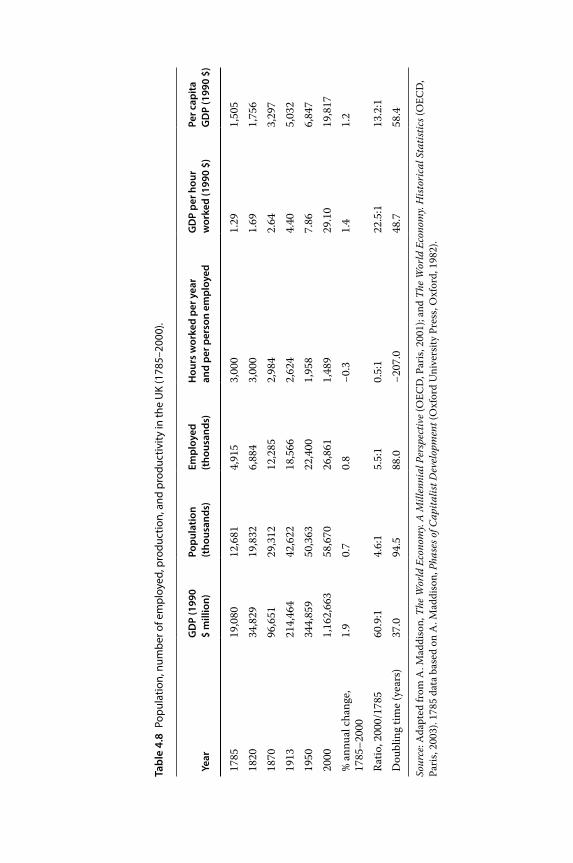
Tabl
e 4.
8 Po
pula
tion,
num
ber o
f em
ploy
ed, p
rodu
ctio
n, a
nd p
rodu
ctiv
ity in
the
UK
(178
5–20
00).
Year
GD
P (1
990
$ m
illio
n)Po
pula
tion
(tho
usan
ds)
Empl
oyed
(t
hous
ands
)H
ours
wor
ked
per y
ear
and
per p
erso
n em
ploy
edG
DP
per h
our
wor
ked
(199
0 $)
Per c
apita
G
DP
(199
0 $)
1785
19,0
8012
,681
4,91
53,
000
1.29
1,50
518
2034
,829
19,8
326,
884
3,00
01.
691,
756
1870
96,6
5129
,312
12,2
852,
984
2.64
3,29
719
1321
4,46
442
,622
18,5
662,
624
4.40
5,03
219
5034
4,85
950
,363
22,4
001,
958
7.86
6,84
720
001,
162,
663
58,6
7026
,861
1,48
929
.10
19,8
17%
ann
ual c
hang
e,
1785
–200
01.
90.
70.
8−0
.31.
41.
2
Ratio
, 200
0/17
8560
.9:1
4.6:
15.
5:1
0.5:
122
.5:1
13.2
:1D
oubl
ing
time
(yea
rs)
37.0
94.5
88.0
−207
.048
.758
.4
Sour
ce: A
dapt
ed fr
om A
. Mad
diso
n, T
he W
orld
Eco
nom
y. A
Mill
enni
al P
ersp
ectiv
e (O
ECD
, Par
is, 2
001)
; and
The
Wor
ld E
cono
my.
Hist
oric
al S
tatis
tics (
OEC
D,
Pari
s, 20
03).
1785
dat
a ba
sed
on A
. Mad
diso
n, P
hase
s of C
apita
list D
evel
opm
ent (
Oxf
ord
Uni
vers
ity P
ress
, Oxf
ord,
198
2).
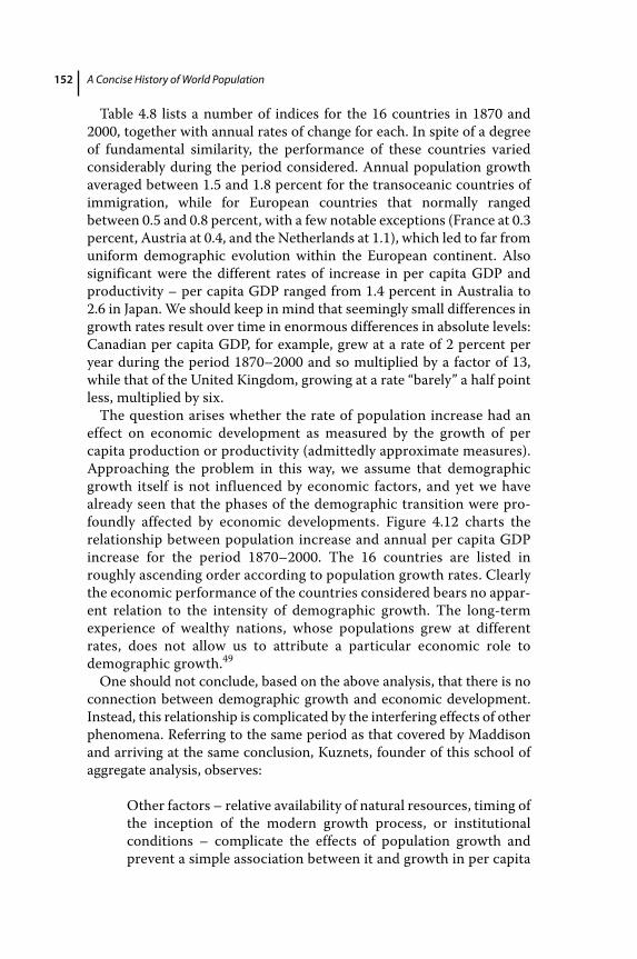
A Concise History of World Population152
Table 4.8 lists a number of indices for the 16 countries in 1870 and 2000, together with annual rates of change for each. In spite of a degree of fundamental similarity, the performance of these countries varied considerably during the period considered. Annual population growth averaged between 1.5 and 1.8 percent for the transoceanic countries of immigration, while for European countries that normally ranged between 0.5 and 0.8 percent, with a few notable exceptions (France at 0.3 percent, Austria at 0.4, and the Netherlands at 1.1), which led to far from uniform demographic evolution within the European continent. Also significant were the different rates of increase in per capita GDP and productivity – per capita GDP ranged from 1.4 percent in Australia to 2.6 in Japan. We should keep in mind that seemingly small differences in growth rates result over time in enormous differences in absolute levels: Canadian per capita GDP, for example, grew at a rate of 2 percent per year during the period 1870–2000 and so multiplied by a factor of 13, while that of the United Kingdom, growing at a rate “barely” a half point less, multiplied by six.
The question arises whether the rate of population increase had an effect on economic development as measured by the growth of per capita production or productivity (admittedly approximate measures). Approaching the problem in this way, we assume that demographic growth itself is not influenced by economic factors, and yet we have already seen that the phases of the demographic transition were profoundly affected by economic developments. Figure 4.12 charts the relationship between population increase and annual per capita GDP increase for the period 1870–2000. The 16 countries are listed in roughly ascending order according to population growth rates. Clearly the economic performance of the countries considered bears no apparent relation to the intensity of demographic growth. The long‐term experience of wealthy nations, whose populations grew at different rates, does not allow us to attribute a particular economic role to demographic growth.49
One should not conclude, based on the above analysis, that there is no connection between demographic growth and economic development. Instead, this relationship is complicated by the interfering effects of other phenomena. Referring to the same period as that covered by Maddison and arriving at the same conclusion, Kuznets, founder of this school of aggregate analysis, observes:
Other factors – relative availability of natural resources, timing of the inception of the modern growth process, or institutional c onditions – complicate the effects of population growth and prevent a simple association between it and growth in per capita
Toward Order and Efficiency 153
product: and population growth itself may have both expansive and depressive effects on the increase in per capita product that differ in their weight in conjunction with other factors.50
Beyond these considerations there is a more general one that can only further complicate the relationship: population and economy are at the same time dependent and independent variables. Economic development, as we have seen, exercised a strong influence on the progress of mortality and fertility during the demographic transition, but, as described in the previous section, the reverse is also true. In an open and integrated system, characterized by significant currents of migration (which served as an important force for maintaining equilibrium in much of the period considered), the long‐term effects of economic and demographic stimuli tend to mitigate and compensate for one another.
Remaining on an aggregate level, the large economic cycles of the modern era can provide us with a few more insights into the population–economy relationship. Keynes, for example, discussing the rate of capital formation in Great Britain between 1860 and 1913, stated: “Thus the increased demand for capital was primarily attributable to the increasing population and to the rising standard of life and only in a minor degree to technical changes of a kind which called for an increasing capitalization
Population
0.0
Aus
tria
Fra
nce
Uni
ted
Kin
gdom
Bel
gium Ita
ly
Sw
eden
Sw
itzer
land
Ger
man
y
Nor
way
Den
mar
k
Fin
land
Japa
n
Net
herla
nds
Uni
ted
Sta
tes
Can
ada
Aus
tral
ia
0.5
1.0
1.5
Per
cent
age
annu
al in
crea
se
2.0
2.5
3.0
GDP per capita
Figure 4.12 Annual rate of increase in population and per capita GDP for 16 industrialized countries (1870–2000).
A Concise History of World Population154
per unit of consumption”; the demographic deceleration of the interwar period presumably influenced the level of demand, creating overproduction and unemployment.51 Hansen was of a similar opinion and attributed 40 percent of capital formation in western Europe and 60 percent in the United States during the second half of the nineteenth century to demographic growth; conversely, he traced the economic crisis of the 1930s to the demographic deceleration of the early part of the century and the consequent slowing of investment.52 It was again Kuznets who attempted to detect a link between demographic and economic cycles in the United States. An increasing standard of living attracted immigration and encouraged nuptiality, accelerating demographic increase. Demographic increase in turn stimulated those investments particularly sensitive to population growth (housing, railroads), but at the expense of other investments in capital goods (machinery and industrial structures). The latter situation negatively affected production and consumption, and so demographic growth, and led to the beginning of another cycle.53
Figure 4.13 records changes (in relation to the previous decade) in population increase (in millions), in GDP increase (in billions of dollars), and in per capita income (in dollars) in the United States for each decade from 1875 to 1955. The trends of these three variables are surprisingly similar.
Returning to Europe, it is difficult to explain the phases of economic growth – expansion preceding World War I, stagnation between the wars, and strong recovery since the 1960s (notably interrupted by the oil crisis of the 1970s) – in terms of demographic factors, which tend to act slowly. Nonetheless, this analysis would be incomplete if it did not take into account several significant demographic factors:
1) The first factor is the geodemographic structure of the European continent (excluding the USSR) and its consequences for spatial politico‐economic organization, indirectly connected with advantages or disadvantages of scale. Prior to World War I, five large nations (Great Britain, France, Germany, Austria‐Hungary, and Italy) dominated the European scene and contained more than three‐quarters of the total European population. The rest of the population was s cattered among a dozen small countries each one with a population of only a few million, plus Spain. After World War I and the Versailles Treaty, Europe was divided into 22 nations, and the large states, with the dismemberment of Austria‐Hungary, were reduced from five to four. The level of continental fragmentation increased, a situation that aggravated the effects of political barriers to the mobility of population and goods.54 After World War II and the “separation” of eastern Europe, compartmentalization (which declined within
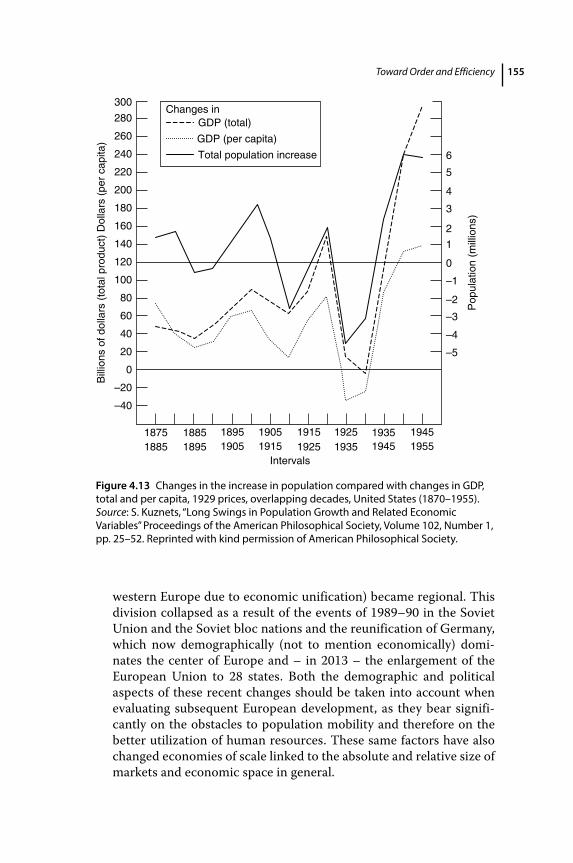
Toward Order and Efficiency 155
western Europe due to economic unification) became regional. This division collapsed as a result of the events of 1989–90 in the Soviet Union and the Soviet bloc nations and the reunification of Germany, which now demographically (not to mention economically) dominates the center of Europe and – in 2013 – the enlargement of the European Union to 28 states. Both the demographic and political aspects of these recent changes should be taken into account when evaluating subsequent European development, as they bear significantly on the obstacles to population mobility and therefore on the better utilization of human resources. These same factors have also changed economies of scale linked to the absolute and relative size of markets and economic space in general.
1875
–40
–20
–5
–4
–3
–2
Pop
ulat
ion
(mill
ions
)
–1
0
1
2
3
4
5
6
0
20
40
60
80
100
120
Bill
ions
of d
olla
rs (
tota
l pro
duct
) D
olla
rs (
per
capi
ta)
140
160
180
200
220
240
260
280
300
1885 189518951905
19051915
19151925
Intervals
1925
Changes inGDP (total)
Total population increase
GDP (per capita)
193519351945
19451955
1885
Figure 4.13 Changes in the increase in population compared with changes in GDP, total and per capita, 1929 prices, overlapping decades, United States (1870–1955). Source: S. Kuznets, “Long Swings in Population Growth and Related Economic Variables” Proceedings of the American Philosophical Society, Volume 102, Number 1, pp. 25–52. Reprinted with kind permission of American Philosophical Society.
A Concise History of World Population156
2) Another important aspect in determining the role of demographic growth in the expansion of demand is the growth of urban areas and above all of large cities, so often the catalysts of development. Urban growth requires large investment in construction and also frequently in high‐tech infrastructure. The 25 European cities that had populations above 500,000 in 1910 had grown in the period 1870–1910 at an annual rate of 1.9 percent; between 1910 and 1940 growth slowed to 0.9 percent and then to 0.3 percent between 1940 and 1970.55 One could make similar observations regarding the non‐European developed countries: while strong in the pre‐World War I period, the driving role of urban growth rapidly declined afterward.
3) Mobility and migration measure the ability of a demo‐economic system to efficiently distribute human resources. From this point of view, recent European history can be divided into three periods. The first ended with the imposition of immigration restrictions by overseas receiving countries in the early 1920s. It was characterized by strong redistribution processes that sent masses of primarily rural population to overseas destinations. At the same time migration between and within European states was also intense. Legislative barriers to migration were few, and the international labor market was relatively fluid and flexible, despite the difficulty and high cost of transportation. The second period, that between the two world wars, was characterized by the closure of extra‐European outlets and the progressive internal compartmentalization of the continent.56 The labor market shrank and became fragmented. The third, post‐World War II phase has been characterized by the “natural” end of emigration outside Europe, by considerable population redistribution within western Europe (sharply divided from the nonmarket‐economy Europe), and by the increasing availability of non‐European labor. Intra‐European migration closes progressively in the 1970s and 1980s as the population reservoir of Mediterranean Europe gradually dries up. But immigration from extra‐European countries becomes a dominant factor, notwithstanding the restrictive policies of most countries. The importance of a mobile and plentiful labor force was underlined by economists like Kindleberger, who attributed to it the rapid economic recovery of western Europe in the immediate postwar period.57
The conclusions to be drawn from this analysis, kept intentionally g eneral, are fairly weak. If nothing else, we can assert that during the nineteenth and twentieth centuries demographic growth did not hinder economic development. In fact, there are indications that the reverse was true. And while maintaining a position of neutrality on the question of the relationship between economic and demographic growth, it is
Toward Order and Efficiency 157
nonetheless the case that those nations that experienced the greatest demographic growth are those that have assumed a leading economic role. A final example may help to clarify this relationship. Between 1870 and 2000 the annual growth rate of per capita GDP in the United States and France was identical (1.9 percent), while the population growth rates were very different (1.5 percent in the United States, 0.3 percent in France). As a result, comparison of the economic dimensions of the two countries, as measured by GDP, has changed from a 1.4:1 ratio (in favor of the United States) in 1870 to 5:1 today. Many will hold that per capita income is what matters and that, under this profile, France has done as well as the United States. But under the geopolitical profile, it is the size of the economy that matters the most. With an economy five times larger, and with the same fraction of GDP, the United States can now send to the poor countries five times more aid than France, in the form of credit, food, medicines, tools, or computers. Or can have five times the number of planes, missiles, and ships to wage a war. One cannot but ask the entirely rhetorical question: Would the United States be the leader of the western world if it had experienced more modest demographic growth?
Notes
1 D. S. Landes, “Technological Change and Development in Western Europe 1750–1914,” in H. J. Habakkuk and M. Postan, eds., Cambridge Economic History (Cambridge University Press, Cambridge, 2nd edn 1965), vol. 6, pt. 1, pp. 274–661.
2 The data in Table 4.1, the concept of multiplier, and the above description of the transition model are Taken from J.‐C. Chesnais, La Transition Démographique [The Demographic Transition] (PUF, Paris, 1986), p. 33; J.‐C. Chesnais, “Demographic Transition Patterns and Their Impact on Age Structure,” Population and Development Review 16:2 (1990).
3 L. Del Panta, Le Epidemie nella Storia Demografica Italiana (Secoli XIV–XIX) [Epidemics in Demographic History (XIV–XIX centuries)] (Loescher, Turin, 1980), pp. 160, 168. C. Ó Gráda, Famine. A Short History (Princeton University Press, Princeton, NJ, 2009).
4 According to the model life tables of Coale and Demeny (A. J. Coale and P. Demeny, Regional Model Life Tables and Stable Populations, Princeton University Press, Princeton, NJ, 1966), for example, taking life expectancies of 27.5 years for women and 25.3 for men (model West), we obtain the following results. The probability that a 40‐year‐old woman lives to 60 is 0.536 and the probability that a 10‐year‐old boy lives to 30 is 0.764. During a 20‐year period, a mother and son aged 40 and 10 present four possibilities: (1) that both survive, the probability for which is
A Concise History of World Population158
0.536 × 0.764 = 0.410; (2) that the mother outlives the son, with a probability of 0.536 × (1 − 0.764) = 0.126; (3) that the son outlives the mother, with a probability of 0.764 × (1 − 0.536) = 0.354; (4) that both die, with a probability of (1 − 0.536) × (1 − 0.764) = 0.110. The sum of the four probabilities of course equals 1. Should the mother survive (probability 0.536), she outlives her son in one case out of four (0.126: 0.536 = 0.235). Given present‐day m ortality, the probability of this happening is about 1 in 60.
5 K. F. Helleiner, “The Population of Europe from the Black Death to the Eve of the Vital Revolution,” in The Cambridge Economic History of Europe (Cambridge University Press, Cambridge, 1967), vol. 4: The Economy of Expanding Europe in the Sixteenth and Seventeenth Centuries, ed. E. E. Rich and C. Wilson.
6 The literature on this subject is vast. I shall limit myself to the following citations: for Italy, Del Panta, Le Epidemie; for England, E. A. Wrigley and R. S. Schofield, The Population History of England, 1541–1871 (Edward Arnold, London, 1981); for Spain, V. Pérez Moreda, Las Crisis de Mortalidad en la España Interior, Siglos XVI–XIX [The Mortality Crisis in the Spanish Interior, XV–XIX Centuries] (Siglo Veintiuno, Madrid, 1980); for France, G. Cabourdin, J.‐N. Biraben, and A. Blum, “Les Crises Démographiques, [Demographic Crises]” in J. Dupâquier, ed., Histoire de la Population Française [History of the French Population] (PUF, Paris, 1988), vol. 2: De la Renaissance à 1789 [From the Renaissance to 1789].
7 On the great microbiological discoveries of the nineteenth century, see G. Penso, La Conquista del Mondo Invisibile (Feltrinelli, Milan, 1973).
8 T. McKeown, The Modern Rise of Population (Edward Arnold, London, 1976).
9 G. Caselli, “Health Transition and Cause‐Specific Mortality,” in R. Schofield, D. Reher, and A. Bideau, eds., The Decline of Mortality in Europe (Oxford University Press, Oxford, 1991).
10 Values of e0 equal to 50 are obtained by linear interpolation (and in some cases extrapolation) of series for the various countries found in L. I. Dublin, A. J. Lotka, and M. Spiegelman, Length of Life (Ronald Press, New York, 1949). For Sweden, Denmark, Belgium, the Netherlands, Switzerland, Australia, and the United States the date at which female life expectancy reached 50 falls between 1880 and 1900; for England, France, and Germany it is between 1900 and 1910; for Finland, Austria, and Italy between 1910 and 1920; for Greece, Hungary, and the USSR after 1920.
11 A. Maddison, Monitoring the World Economy 1820–1992 (OECD, Paris, 1995). GDP (Gross Domestic Product) and GDP per capita used in this and in the next chapter are in “1990 international dollars” (or 1990
Toward Order and Efficiency 159
Geary–Khamis dollars, from the names of the scholars who developed the methodology). These are known also as PPP (Purchasing Power Parity) dollars. A PPP dollar is an abstract measure that, taking into consideration the fact that prices change across time and space, “buys” the same fraction of well‐being and therefore is historically and geographically comparable. In practice, the “international dollar” has many limitations either intrinsic to the quantitative material available (quite scarce and often unreliable, particularly for remote times) or because the range of goods and services produced and available for consumption is in continuous change. See pp. 162–9 of Maddison’s book. For the list of the 16 countries, see Table 4.5.
12 The most significant of these is that the two variables are not independent from one another: while it is true that mortality depends in part on well‐being, it is also the case that there would not have been material progress without mortality decline.
13 There exists, of course, fertility outside of marriage, generally (and improperly) called illegitimate. Historically, levels of illegitimate fertility in the West have been insignificant as (at least until the last few decades) the vast majority of reproduction has taken place within the context of marriage.
14 It is a conceptually subtle distinction that separates voluntary from nonvoluntary fertility control. Demographers call fertility that is not voluntarily controlled “natural fertility.” Its level can vary considerably as a function of the behavior of couples or mothers (sexual taboos, frequency of intercourse, length of breast‐feeding, and so on – see Chapter 1, Section 4). Nonetheless, these types of behavior are presumably “structural” and do not reflect the desire of couples to achieve a particular family size; procreational behavior does not vary as a function of the number of children already born. Voluntary fertility control by means of contraception or coitus interruptus, on the other hand, has as its aim the production of a certain number of children. Control is practiced above all by couples who have reached the desired number, so that reproductive behavior tends to change as a function of children born. A decline in the average age of the mother at last birth or in fertility at the youngest ages is a sign of fertility control in a population; both situations lead to a change in the “shape” of the fertility curve by age.
15 M. Livi‐Bacci, “Social‐Group Forerunners of Fertility Control in Europe,” in A. J. Coale and S. C. Watkins, eds., The Decline of Fertility in Europe (Princeton University Press, Princeton, NJ, 1986).
16 Urban fertility was generally lower than rural, though this was due in part to the particular makeup of the urban population and its high mobility. However, contrary to the model of slower rural decline, fertility began to drop in some areas of Hungary from the late‐eighteenth century. See R. Andorka,
A Concise History of World Population160
“La prévention des Naissances en Hongrie dans la Région Ormansag Depuis la Fin du XVIIIe Siècle [Birth Control in Hungary in the Ormansag Region since the End of the Eighteenth Century],” Population 26 (1971).
17 The general aims, characteristics, and results of this study, directed by Ansley Coale and coordinated by the Office of Population Research at Princeton, are summarized in Coale and Watkins, Decline of Fertility. The graphs in Figure 4.6 (a–e) include points for the following countries: Belgium, Denmark, England and Wales, Finland, France, Germany, Hungary, Ireland, Italy, the Netherlands, Norway, Portugal, Scotland, Spain, Sweden, and Switzerland.
18 The indices Im, If, Ig (indices of the proportion of women of childbearing age who are married, general fertility, and legitimate fertility), and Ih (a similar index of illegitimate fertility not discussed here) are calculated in the following manner; fi, gi, and hi represent, respectively, total births, legitimate births, and illegitimate births per woman of age interval i. Similarly, wi, mi, and ui represent total women, married women, and unmarried women in the same age interval. Fi is the fertility coefficient for the model population, namely Hutterite women married in the period 1921–30, a group notable for having the highest fertility ever recorded in a regularly constituted population. Given the above information, the f ollowing indices can be calculated:
General fertility I f w F wi i i if / [1]
Legitimate fertility I g m F mi i i ig / [2]
Illegitimate fertility I h u F ui i i ih / [3]
Proportion of women married I F m F wi i i im / [4]
The numerators of equations 1, 2, and 3 are, respectively, the total births, legitimate births, and illegitimate births of the population studied. The values of Fi are: ages 15–19 = 0.300, 20–24 = 0.550, 25–29 = 0.502, 30–34 = 0.447, 35–39 = 0.406, 40–44 = 0.222, 45–49 = 0.061. The four indices are related by the following equation: If = Ig × Im + Ih × (1 − Im). When Ih is very low, say below 0.05 (or 5 percent), as has traditionally been the case for all western populations, then the index of general fertility closely approximates Ig × Im. All the indices have values below 1. In the case of Ig the value of the index represents the ratio between the legitimate fertility of the population studied and the theoretical maximum of the Hutterites. Values below 0.6 generally indicate a degree of voluntary fertility control.
19 Among the results of the Princeton study are maps of fertility and nuptiality trends from the second half of the nineteenth century to 1960. See Coale and Watkins, Decline of Fertility. For more detailed
Toward Order and Efficiency 161
“geography,” see the national monographs, all published by the Princeton University Press, for the following countries: France (E. van de Walle), Great Britain (M. Teitelbaum), Germany (M. Knodel), the former USSR (B. Anderson, A. J. Coale, and E. Harm), Italy (M. Livi‐Bacci), Belgium (R. Lesthaeghe), and Portugal (M. Livi‐Bacci).
20 Several authors believe that in the long term that fertility will hover around two, in keeping with the mean number of children that women and couples declare to want, or expect to have or consider as ideal – as shown repeatedly by surveys. Substantial deviations from this pattern would be mainly the consequence of changes in the “tempo” of fertility, due to transitory factors. On this position is J. Bongaarts, “Fertility and Reproductive Preferences in Post‐Transitional Societies,” Population and Development Review 27:Suppl. (2001). Others – among them this author – are of a different opinion and argue that societies may adjust, for long periods, to patterns of fertility that are structurally very low, as the cases of Germany and Italy demonstrate. Some more has to be said about the concept of “replacement fertility.” Fertility is at “replacement level” when each generation of women exactly replaces the previous one, implying that a newborn girl gives birth to one daughter on average during her lifetime. Replacement fertility exceeds two because more boys are born than girls (the sex ratio at birth is 1.05/1.06 boys:1 girl) and also because children who die before reaching reproductive age must be replaced with additional births. The higher mortality, the higher replacement fertility. This now is fractionally lower than 2.1 in developed countries and stands at 2.4 in developing ones. See also note 16, Chapter 1. For the view that the era of very low fertility is at the end and that a turning point is in the making, see J. R. Goldstein, T. Sobotka, and A. Jasilioniene, “The end of ‘lowest‐low’ fertility,” Population and Development Review 35:4 (December 2009).
21 The values of TFR used here are “period” rates as opposed to the “cohort” rates used in Table 4.7. Period rates are calculated by combining fertility levels for women of different ages at the same date (and so born on d ifferent dates and having different fertility histories) and so emphasize the temporary influence of economic factors.
22 A. Maddison, Monitoring the World Economy, 1820–1922 (OECD, Paris, 1995), pp. 61–4.
23 K. O’Rourke and J. G. Williamson, Globalization and History, the Evolution of a Nineteenth Century Atlantic Economy (MIT Press, Cambridge, MA., 1999).
24 Chesnais, La Transition Démographique, p. 164.25 By combining US immigration statistics with census results (which
asked for the nationality of those surveyed), I have been able to calculate that between 1880 and 1950, 50.2 percent of Italian immigrants returned to Italy after stays of varying lengths. M. Livi‐Bacci,
A Concise History of World Population162
L’Immigrazione e l’assimilazione degli Italiani negli Stati Uniti [Immigration and Assimilation of Italians in the United States] (Giuffrè, Milan, 1961), pp. 34 – 5. In order to calculate the present‐day population descended from net Italian migration in the period 1861–1961, I applied the Italian growth rate for each decade to the net migration for the same period, assuming that it was maintained (by both the first migrants and their descendants) up until 1981.
26 Chesnais, La Transition Démographique, pp. 169–72.27 P. Bairoch, International Historical Statistics, vol. 1: The Working
Population and its Structure (New York, 1969).28 D. Grigg, The Transformation of Agriculture in the West (Blackwell,
Oxford, 1992), Table 4.2, p. 35.29 Grigg, Transformation of Agriculture in the West, Table 2.2, p. 19.30 See D. S. Massey, J. Arango, G. Hugo, A. Kouaouci, A. Pellegrino, and
J. E. Taylor, Worlds in Motion: Understanding International Migration at the End of the Millennium (Oxford University Press, Oxford, 1998). D. J. Hatton and J. G. Williamson, The Age of Mass Migration: Causes and Economic Impact (Oxford University Press, Oxford, 1998).
31 A typical case is that of Venetia, which, in the 1920s, was the last region of north‐central Italy to initiate fertility control. Legitimate fertility (Ig) increased considerably in the period just prior to the onset of decline (almost 20 percent between 1881 and 1911). Factors influencing the increase included improved living conditions and the elimination of p ellagra, a vitamin‐deficiency‐related disease resulting from excessive dependence on corn (maize). See M. Livi‐Bacci, “Fertility, Nutrition and Pellagra: Italy during the Vital Revolution,” Journal of Interdisciplinary History 16 (Winter, 1986).
32 It is, however, generally considered obvious that the increased survivorship of the twentieth century is responsible for the demographic aging of the population – that is, the increased proportion of old people. This aging has, in fact, been due exclusively to the progressive decline of fertility as a result of which the younger levels of the age structure have not been sufficiently replenished. Moreover, one can show that improved survivorship was proportionately more significant for younger age groups than for older and so created a greater increase, all things being equal, among the young than the old; the age structure actually became younger. The situation today and in the near future, however, is different. Improvements in survivorship will almost exclusively benefit the old (there being virtually no room left for improvement at the younger ages). As a result further mortality decline will contribute to population aging. Historically, however, this has not been the case.
33 Obviously fertility alone does not determine the change in family size. Survivorship, age at which the children leave home, widowhood and
Toward Order and Efficiency 163
second marriages, the frequency of extended families (composed of more than one biological nucleus), and cohabitation of nonrelated persons are also factors determining family size.
34 A population with fixed fertility and mortality behavior ultimately achieves a fixed‐age structure (determined by this behavior) as well as fixed crude birth, death, and growth rates. A theoretical population of this sort is called a “stable” population. In Table 4.6, the parameters reported refer to the stable populations, which would be produced by Italian mortality and fertility behavior in 1881 and 1981.
35 J. A. Schumpeter, Capitalism, Socialism, and Democracy (Harper & Brothers, New York, 2nd edn 1947), p. 83.
36 J. Simon, The Economics of Population Growth (Princeton University Press, Princeton, NJ, 1976); J. Simon, Theory of Population Economics (Blackwell, Oxford, 1986).
37 Y. Hayami and V. W. Ruttan, Population Growth and Agricultural Productivity (Johns Hopkins University Press, Baltimore, MD, 1985).
38 W. S. Jevons, The Coal Question (Macmillan, London, 1865).39 Club of Rome, The Limits to Growth (Universe Books, New York, 1972).40 Maddison, Phases, p. 48. A similar trend has taken place in Great
Britain, where the ratio declines from 2.55 TPE per $1,000 of production in 1855 to 0.99 in 1979. For recent trends in the United States and in other major countries, see http://data. worldbank.org/indicator/EG.GDP. PUSE.KO.PP.KD/countries?page = 5 [accessed July 21, 2016].
41 A. Marshall, Principles of Economics (Macmillan, London, 1920), pp. xv–xvi. A bushel is equivalent to 35.2 liters.
42 These arguments are developed in S. Kuznets, Modern Economic Growth (Yale University Press, New Haven, CT, 1966), p. 57.
43 J. J. Spengler, Facing Zero Population Growth (Duke University Press, Durham, NC, 1978), pp. 136–9.
44 E. F. Denison, Accounting for the United States’ Economic Growth (Brookings Institution, Washington, DC, 1974), pp. 71–5; and by the same author: Why Growth Rates Differ (Brookings Institution, Washington, DC, 1967), pp. 232–3.
45 E. A. G. Robinson, ed., Economic Consequences of the Size of Nations (Macmillan, London, 1960), p. xxii of Robinson’s Introduction. A. Alesina and A. Spolaore, The Size of Nations (MIT Press, Cambridge, MA, 2003).
46 J. M. Keynes, “Some Economic Consequences of a Declining Population,” Eugenics Review 4:3 (April 1937). These same ideas were stated much more explicitly in J. R. Hicks’s review of Keynes, “Mr. Keynes’ Theory of Employment,” cited in Spengler, Facing Zero Population Growth, p. 62: “Expectation of a continually expanding market, made possible by increasing population, is a fine thing for keeping up the spirit of entrepreneurs. With increasing population
A Concise History of World Population164
investment can go roaring ahead, even if invention is rather stupid; increasing population is therefore actually favorable to employment.”
47 S. Kuznets, “Population Change and Aggregate Output” (NBER report), in Demographic and Economic Change in Developed Countries (Princeton University Press, Princeton, NJ, 1960), pp. 329–30.
48 These series, in 1990 international dollars, are found in Maddison, Monitoring the World Economy. See also note 11 of this chapter.
49 The lack of a clear relationship is evident even when examining s eparately the three subperiods. The correlation coefficients between the rates of variation for population and GDP are: 1870–1913, + 0.003; 1913–50, +0.180; 1950–87, −0.220; 1970–87, −0.119.
50 Kuznets, Modern Economic Growth, p. 68.51 Keynes, “Some Economic Consequences,” p. 15.52 Cited in Spengler, Facing Zero Population Growth, p. 64.53 S. Kuznets, Economic Growth and Structure (Norton, New York, 1965),
pp. 345–9. For refinement and discussion of the Kuznets model see R. A. Easterlin, “Economic– Demographic Interactions and Long Swings in Economic Growth,” American Economic Review 56 (1966).
54 I. Svennilson, Growth and Stagnation in the European Economy (United Nations Economic Commission for Europe, Geneva, 1954), pp. 67–8.
55 The population of these 25 cities was 13.1 million in 1870, 28.4 million in 1910, 37.7 million in 1940, and 41.4 million in 1970. Data taken from B. R. Mitchell, European Historical Statistics (Macmillan, London, 1980).
56 D. Kirk, Europe’s Population in the Interwar Years (League of Nations, Princeton University Press, Princeton, NJ, 1946), pp. 97–125.
57 C. P. Kindleberger, Europe’s Postwar Growth (Harvard University Press, Cambridge, MA, 1967). See also M. Livi‐Bacci and G. Tapinos, “Economie et Population,” in J.‐P. Bardet and J. Dupâquier, eds., Histoire de la Population de l’Europe [The History of the Population of Europe], vol. 3: Les Temps Incertains, 1914–98 [Uncertain Times: 1904–98] (Fayard, Paris, 1998).
Further Reading
J. P. Bardet and J. Dupâquier, eds., Histoire des Populations de l’Europe [The History of European Populations], 3 vols. (Fayard, Paris, 1997–9).
A. J. Coale and S. C. Watkins, The Decline of Fertility in Europe (Princeton University Press, Princeton, NJ, 1986).
I. Ferenczi and W. F. Wilcox, International Migration, 2 vols. (NBER, New York, 1929–31).
M. W. Flinn, The European Demographic System 1500–1820 (Johns Hopkins University Press, Baltimore, MD, 1981).

Toward Order and Efficiency 165
M. Haines and R. H. Steckel, A Population History of North America (Cambridge University Press, Cambridge and New York, 2000).
T. J. Hatton and J. G. Williamson, The Age of Mass Migration: Causes and Economic Impact (Oxford University Press, Oxford, 1998).
M. Livi‐Bacci, The Population of Europe: A History (Blackwell, Oxford, 1999).
C. Ó Gráda, Famine. A Short History (Princeton University Press, Princeton, NJ, 2009).
R. Schofield, D. Reher, and A. Bideau, eds., The Decline of Mortality in Europe (Clarendon Press, Oxford, 1991).
E. A. Wrigley and R. S. Schofield, The Population History of England 1541–1871: A Reconstruction (Edward Arnold, London, 1981).
167
A Concise History of World Population, Sixth Edition. Massimo Livi-Bacci. © 2017 John Wiley & Sons Ltd. Published 2017 by John Wiley & Sons Ltd.
The Populations of Poor Countries
5.1 An Extraordinary Phase
As the rich countries of the world complete a phase of population expan-sion, the poor countries have embarked upon an extraordinary and n onrepeatable one of their own. The characteristics of this growth cycle are well described by the dry figures charting recent demographic growth in the so‐called less‐developed countries – namely those countries whose populations live, by western standards, in poverty.1 The 1900 population of the poor countries, about 1 billion, had multiplied sixfold by the year 2015; during the twentieth century these countries matched the expan-sion of the rich countries in the two centuries following the Industrial Revolution. That speed of growth is extraordinary. Between 1900 and 1920, we estimate the growth rate of the poor countries was about 0.6 percent per year; this rate doubled for the period 1920–50 (about 1.2 percent) and once again in the 1960s when the maximum rate of 2.4 percent was reached, followed by gradual decline in the five decades from 1970 (Table 5.1). By contrast, the western countries (Europe and its overseas projections) only rarely exceeded a rate of 1 percent during their two centuries of expansion. Since the 1950s the poorer part of the world has grown at twice that rate.
The reasons for this difference are, on the surface, rather simple, though the underlying reality is complex. In the rich world the demo-graphic transition came about slowly as a result of a gradual decline in mortality, accompanied by a similar decline in fertility. Slow mortality decline, as described in the previous chapter, was the result of an accu-mulation of knowledge, especially medical knowledge, which helped to bring infectious diseases under control – beginning at the end of the nineteenth century and continuing up to the present day. In the poor world mortality levels remained high until recently. In 1950, for e xample, average life expectancy in poor countries was still around 40.
5

A Concise History of World Population168
However, from the mid‐twentieth century onward, that knowledge slowly accumulated by the rich countries was rapidly transferred to the poor ones and mortality dropped dramatically. Fertility, largely dependent upon slowly changing cultural factors, either did not follow the trend in mortality or else did so slowly, and the two indices assumed widely divergent levels.
As mentioned above, the apparent simplicity of this process is mislead-ing. The poor world is divided into societies characterized by vastly dif-ferent environmental, cultural, and political settings, and these differences are reflected in the demographic behavior of individual populations. Nor has the poor world been isolated from the rich, so that a degree of knowledge and technology transfer took place before the 1950s. However, taking these factors into account, the fact remains that demographic change in the poor world in recent decades has on average proceeded rap-idly when compared to the path previously followed by the rich (Figure 5.1).
Table 5.2 describes global demographic diversity as measured by a num-ber of now‐familiar indices (for 1950–5 and 2010–15 for poor and rich, for large continental areas, and for India and China – these last two coun-tries contain half of the total population of the poor world). These data permit us to make three general observations regarding the distinctive characteristics of rich and poor countries, the changing demography of the poor countries during recent decades, and interregional differences.
Table 5.1 World population, rich and poor countries (1900–2020).
Population (millions) Annual rate of growth (%) % share
Year Rich Poor World Rich Poor World Rich Poor World
1900 563 1071 1634 – – – 34.5 65.5 1001920 654 1203 1857 0.75 0.58 0.64 35.2 64.8 1001930 727 1309 2036 1.06 0.84 0.92 35.7 64.3 1001940 794 1473 2267 0.9 1.2 1.1 35.0 65.0 1001950 813 1712 2525 0.2 1.5 1.1 32.2 67.8 1001960 915 2103 3018 1.2 2.1 1.8 30.3 69.7 1001970 1008 2675 3682 1.0 2.4 2.0 27.4 72.6 1001980 1082 3358 4440 0.7 2.3 1.9 24.4 75.6 1001990 1144 4165 5310 0.6 2.2 1.8 21.5 78.5 1002000 1189 4938 6127 0.4 1.7 1.4 19.4 80.6 1002010 1233 5696 6930 0.4 1.4 1.2 17.8 82.2 1002020 1266 6492 7758 0.3 1.3 1.1 16.3 83.7 100
Source: UN estimates; for 1900 author’s estimate.
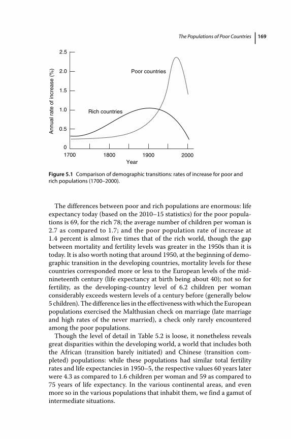
The Populations of Poor Countries 169
The differences between poor and rich populations are enormous: life expectancy today (based on the 2010–15 statistics) for the poor popula-tions is 69, for the rich 78; the average number of children per woman is 2.7 as compared to 1.7; and the poor population rate of increase at 1.4 percent is almost five times that of the rich world, though the gap between mortality and fertility levels was greater in the 1950s than it is today. It is also worth noting that around 1950, at the beginning of demo-graphic transition in the developing countries, mortality levels for these c ountries corresponded more or less to the European levels of the mid‐nineteenth century (life expectancy at birth being about 40); not so for fertility, as the developing‐country level of 6.2 children per woman considerably exceeds western levels of a century before (generally below 5 children). The difference lies in the effectiveness with which the European populations exercised the Malthusian check on marriage (late marriage and high rates of the never married), a check only rarely encountered among the poor populations.
Though the level of detail in Table 5.2 is loose, it nonetheless reveals great disparities within the developing world, a world that includes both the African (transition barely initiated) and Chinese (transition com-pleted) populations: while these populations had similar total fertility rates and life expectancies in 1950–5, the respective values 60 years later were 4.3 as compared to 1.6 children per woman and 59 as compared to 75 years of life expectancy. In the various continental areas, and even more so in the various populations that inhabit them, we find a gamut of intermediate situations.
1700 1800
Rich countries
Poor countries
Ann
ual r
ate
of in
crea
se (
%)
2.5
2.0
1.5
1.0
0.5
0
1900Year
2000
Figure 5.1 Comparison of demographic transitions: rates of increase for poor and rich populations (1700–2000).
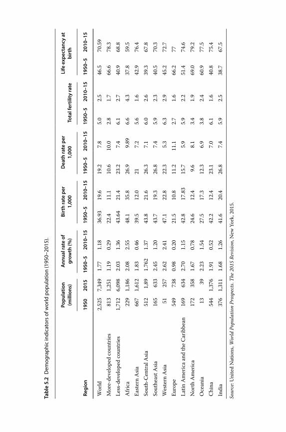
Tabl
e 5.
2 D
emog
raph
ic in
dica
tors
of w
orld
pop
ulat
ion
(195
0–20
15).
Regi
on
Popu
latio
n (m
illio
ns)
Ann
ual r
ate
of
grow
th (%
)Bi
rth
rate
per
1,
000
Dea
th ra
te p
er
1,00
0To
tal f
ertil
ity
rate
Life
exp
ecta
ncy
at
birt
h
1950
2015
1950
–520
10–1
519
50–5
2010
–15
1950
–520
10–1
519
50–5
2010
–15
1950
–520
10–1
5
Wor
ld2,
525
7,34
91.
771.
1836
.93
19.6
19.2
7.8
5.0
2.5
46.5
70.5
9M
ore‐
deve
lope
d co
untr
ies
813
1,25
11.
190.
2922
.411
.110
.610
.02.
81.
766
.678
.3Le
ss‐d
evel
oped
cou
ntrie
s1,
712
6,09
82.
031.
3643
.64
21.4
23.2
7.4
6.1
2.7
40.9
68.8
Afr
ica
229
1,18
62.
082.
5548
.135
.826
.99.
896.
64.
337
.859
.5Ea
ster
n A
sia
667
1,61
21.
830.
4639
.512
.021
7.2
5.6
1.6
42.9
76.4
Sout
h‐C
entr
al A
sia
512
1,89
1.76
21.
3743
.821
.626
.37.
16.
02.
639
.367
.8So
uthe
ast A
sia
165
633
2.45
1.20
43.7
19.3
26.8
7.4
5.9
2.3
40.5
70.3
Wes
tern
Asi
a51
257
2.62
2.41
47.1
22.8
22.3
5.3
6.3
2.9
45.2
72.7
Euro
pe54
973
80.
980.
2021
.510
.811
.211
.12.
71.
666
.277
Latin
Am
eric
a an
d th
e C
arib
bean
169
634
2.70
1.15
42.8
17.8
315
.75.
95.
92.
251
.474
.6N
orth
Am
eric
a17
235
81.
670.
7824
.612
.49.
68.
13.
41.
969
.079
.2O
cean
ia13
392.
231.
5427
.517
.312
.36.
93.
82.
460
.977
.5C
hina
544
1,37
61.
910.
5242
.212
.423
.17.
06.
11.
640
.875
.4In
dia
376
1,31
11.
681.
2641
.620
.426
.87.
45.
92.
538
.767
.5
Sour
ce: U
nite
d N
atio
ns, W
orld
Pop
ulat
ion
Pros
pect
s. Th
e 201
5 Re
visio
n, N
ew Y
ork,
201
5.
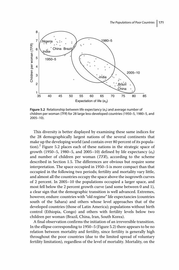
The Populations of Poor Countries 171
This diversity is better displayed by examining these same indices for the 28 demographically largest nations of the several continents that make up the developing world (and contain over 80 percent of its popula-tion).2 Figure 5.2 places each of these nations in the strategic space of growth (1950–5, 1980–5, and 2005–10) defined by life expectancy (e0) and number of children per woman (TFR), according to the scheme described in Section 1.5. The differences are obvious but require some interpretation. The space occupied in 1950–5 is more compact than that occupied in the following two periods; fertility and mortality vary little, and almost all the countries occupy the space above the isogrowth curves of 2 percent. In 2005–10 the populations occupied a larger space, and most fell below the 2 percent growth curve (and some between 0 and 1), a clear sign that the demographic transition is well advanced. Extremes, however, endure: countries with “old regime” life expectancies (countries south of the Sahara) and others whose level approaches that of the d eveloped countries (those of Latin America); populations without birth control (Ethiopia, Congo) and others with fertility levels below two c hildren per woman (Brazil, China, Iran, South Korea).
A final observation confirms the initiation of an irreversible transition. In the ellipse corresponding to 1950–5 (Figure 5.2) there appears to be no relation between mortality and fertility, since fertility is generally high throughout the poor countries (due to the limited spread of voluntary fertility limitation), regardless of the level of mortality. Mortality, on the
351
2
3
4
5
6
7
8
40 45 50 55 60
India
Brazil
2005–10
1980–5Nigeria
China BrazilIndia
1950–5
Chi
ldre
n pe
r w
oman
(TF
R)
China
Expectation of life (e0)
65 70 75 80 85
Figure 5.2 Relationship between life expectancy (e0) and average number of children per woman (TFR) for 28 large less‐developed countries (1950–5, 1980–5, and 2005–10).
A Concise History of World Population172
other hand, had dropped in many countries as a result of the massive infusion of knowledge and technology from the 1940s onward. At the later date (2005–10) there is a clear and negative correlation between e0 and TFR, as the high‐life‐expectancy countries are also those with reduced fertility. This came about in part because increased material well‐being influences life expectancy and fertility in opposite directions, but also because improved survival has begun to have a direct influence on fertility, making high levels of the latter unnecessary and more expen-sive. In general, once this process has begun, it tends to perpetuate itself until mortality has completed its decline.
5.2 The Conditions of Survival
Reduced mortality and establishment of the chronological age‐linked succession of death are prerequisites to development. Moreover, a reduc-tion in infant and child mortality is one of the necessary conditions for fertility decline and the shift from a regime of demographic “waste” to one of demographic “economy.” Beyond these fairly simple observations, we need to expand somewhat the general discussion of poor‐world mor-tality decline.3 First, we should consider the reasons behind the different rates of survivorship improvement for the various poor populations, which as a whole increased life expectancy during the half‐century between the early 1950s and the beginning of the new millennium at a rate of 5 months per calendar year; regional rates ranged from less than 3 months per year in Africa to 7 months in China, and the differences are greater still if we consider smaller areas.
Survivorship improvement is achieved, first of all, by means of the reduction of infant and child mortality. The United Nations4 estimates that the probability of a newborn dying before his or her fifth birthday was 56 per 1,000 in 2010–5 for the less‐developed countries as a whole, but variation among regions was great: 99 per 1,000 in sub‐Saharan Africa, 55 in southern central Asia, 13 in eastern Asia, 26 in Latin America. By comparison, this level in the rich countries is barely 60 per 1,000. If the other countries of the poor world were to reduce their infant and child mortality to the level of eastern Asia (41 per 1,000), life expec-tancy would increase by 5 years in Africa and two in southern Asia.5 In other words, elimination of infant mortality differences would eliminate much of the disparity in life expectancy and so is a primary objective in the quest for improved survivorship: its reduction not only represents a considerable decline in general mortality, but also favors the moderniza-tion of reproductive behavior and improves the level of health at an age crucial to the development and subsequent efficiency of the survivors.
The Populations of Poor Countries 173
The causes of high infant mortality are many and complex: from infectious diseases typical of infancy (measles, diphtheria, whooping cough, polio, tetanus); to a high incidence of diarrhea and gastroenteritis resulting from poor sanitation; to the combined action of malnutrition, poverty, and infection; to the existence of vast malarial areas. With reference to children below 5 years of age living in Sub‐Saharan Africa (2013), 3 percent of deaths are from HIV/AIDS, 15 percent from diarrhea, and 15 percent from malaria. There are solutions to all of these problems: the diseases typical of infancy can be combated with programs of vaccina-tion and immunization; diarrhea and gastroenteritis with improved environmental conditions and hygiene; malaria with disinfestation; and malnutrition with programs of diet supplementation and, in many areas, by discouraging early weaning. When illnesses do occur, medical inter-vention can often prevent their lethality; in many instances diarrhea, which kills by repeatedly attacking and dehydrating the infant, can be cured by simple rehydration methods administered by family members.6 There are solutions, but only providing that the material resources, t echnical knowledge, and collective and individual awareness necessary to implement them – that is to say, education and development – exist.
A clear, if summarized, picture of the conditions accompanying infant mortality is provided by Table 5.3, which records several health indices for selected countries. High infant and child mortality go hand in hand with lack of professional assistance at delivery, low immunization, and a high incidence of stunted growth. Figure 5.3 shows the relationship, for 53 poor countries, between mortality at ages 0–4 and the percentage of the population served by adequate sanitation systems (sewage etc.); the inverse correlation is quite evident.
The complexity of the causes of high infant mortality makes interven-tion difficult when attempting to pass from a “medium” level (the result of initial progress) to a low one like that of the developed countries. I shall return to this question after having discussed the general mortality situation for the various populations, which is most concisely expressed by life expectancy (e0). In Figure 5.4, life expectancy is compared with the classic index of well‐being – per capita GDP (in international dol-lars) – for 28 poor countries.7 As can be seen from the figure, this rela-tionship is similar to that for the western countries (see Chapter 4, Figure 4.4): there is a big increase in life expectancy as per capita GDP increases from very low levels, but a gradual attenuation of survivorship improvement with subsequent increases in production. In other words, the growth of material well‐being is progressively less effective at increas-ing life expectancy. This relationship is in keeping with an initial phase of considerable mortality reduction linked to the introduction of relatively inexpensive and large‐scale technology: antibiotics, DDT disinfestation,
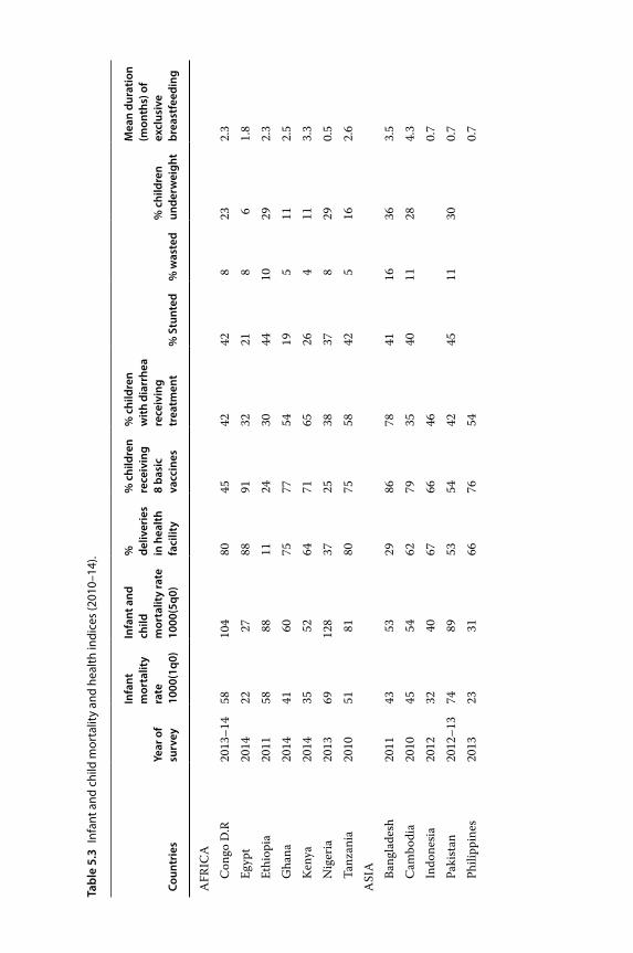
Tabl
e 5.
3 In
fant
and
chi
ld m
orta
lity
and
heal
th in
dice
s (2
010–
14).
Coun
trie
sYe
ar o
f su
rvey
Infa
nt
mor
talit
y ra
te
1000
(1q0
)
Infa
nt a
nd
child
m
orta
lity
rate
10
00(5
q0)
%
deliv
erie
s in
hea
lth
faci
lity
% c
hild
ren
rece
ivin
g 8
basi
c va
ccin
es
% c
hild
ren
with
dia
rrhe
a re
ceiv
ing
trea
tmen
t%
Stu
nted
% w
aste
d%
chi
ldre
n un
derw
eigh
t
Mea
n du
ratio
n (m
onth
s) o
f ex
clus
ive
brea
stfe
edin
g
AFR
ICA
Con
go D
.R20
13–1
458
104
8045
4242
823
2.3
Egyp
t20
1422
2788
9132
218
61.
8Et
hiop
ia20
1158
8811
2430
4410
292.
3G
hana
2014
4160
7577
5419
511
2.5
Ken
ya20
1435
5264
7165
264
113.
3N
iger
ia20
1369
128
3725
3837
829
0.5
Tanz
ania
2010
5181
8075
5842
516
2.6
ASI
A Bang
lade
sh20
1143
5329
8678
4116
363.
5C
ambo
dia
2010
4554
6279
3540
1128
4.3
Indo
nesi
a20
1232
4067
6646
0.7
Paki
stan
2012
–13
7489
5354
4245
1130
0.7
Phili
ppin
es20
1323
3166
7654
0.7
LAT
IN A
MER
ICA
Col
ombi
a20
1016
1995
6861
131
31.
8H
aiti
2012
5888
3845
5722
511
1.7
Peru
2012
1721
8673
3718
13
4.2
Dom
inic
an R
epub
lic20
1327
3199
5252
72
40.
4H
ondu
ras
2011
–12
2429
8585
6022
17
0.7
Sour
ce: T
he D
HS
Prog
ram
, http
://w
ww.
dhsp
rogr
am.c
om/ [
extr
acte
d Fe
brua
ry 7
, 201
6].
Not
es: I
ndic
ator
s ref
er to
the
the
3 ye
ars p
rece
ding
the
surv
ey; i
nfan
t mor
talit
y re
fers
to th
e 5
year
s pre
cedi
ng th
e su
rvey
; the
ant
hrop
omet
ric in
dica
tors
refe
r to
the
perc
ent
of c
hild
ren
2 st
anda
rd d
evia
tions
bel
ow th
e m
ean.
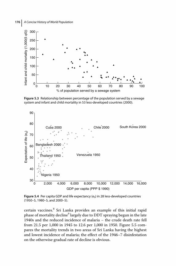
A Concise History of World Population176
certain vaccines.8 Sri Lanka provides an example of this initial rapid phase of mortality decline9 largely due to DDT spraying begun in the late 1940s and the reduced incidence of malaria – the crude death rate fell from 21.5 per 1,000 in 1945 to 12.6 per 1,000 in 1950. Figure 5.5 com-pares the mortality trends in two areas of Sri Lanka having the highest and lowest incidence of malaria; the effect of the 1946–7 disinfestation on the otherwise gradual rate of decline is obvious.
00
50
100
150
200
Infa
nt a
nd c
hild
mor
talit
y (1
,000
(5 q
0))
250
300
10 20 30 40 50% of population served by a sewage system
60 70 80 90 100
Figure 5.3 Relationship between percentage of the population served by a sewage system and infant and child mortality in 53 less‐developed countries (2000).
Chile 2000
Venezuela 1950
300 2,000 4,000 6,000 8,000
GDP per capita (PPP $ 1990)
10,000 12,000 14,000 16,000
40
50
60
Exp
ecta
tion
of li
fe (
e 0)
70
80
90
Thailand 1950
Bangladesh 2000
Nigeria 1950
Cuba 2000 South Korea 2000
Figure 5.4 Per capita GDP and life expectancy (e0) in 28 less‐developed countries (1950–5, 1980–5, and 2000–5).
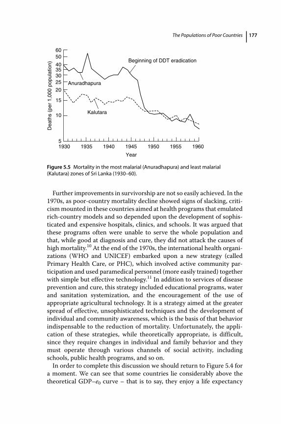
The Populations of Poor Countries 177
Further improvements in survivorship are not so easily achieved. In the 1970s, as poor‐country mortality decline showed signs of slacking, criti-cism mounted in these countries aimed at health programs that emulated rich‐country models and so depended upon the development of sophis-ticated and expensive hospitals, clinics, and schools. It was argued that these programs often were unable to serve the whole population and that, while good at diagnosis and cure, they did not attack the causes of high mortality.10 At the end of the 1970s, the international health organi-zations (WHO and UNICEF) embarked upon a new strategy (called Primary Health Care, or PHC), which involved active community par-ticipation and used paramedical personnel (more easily trained) together with simple but effective technology.11 In addition to services of disease prevention and cure, this strategy included educational programs, water and sanitation systemization, and the encouragement of the use of a ppropriate agricultural technology. It is a strategy aimed at the greater spread of effective, unsophisticated techniques and the development of individual and community awareness, which is the basis of that behavior indispensable to the reduction of mortality. Unfortunately, the appli-cation of these strategies, while theoretically appropriate, is difficult, since they require changes in individual and family behavior and they must operate through various channels of social activity, including schools, public health programs, and so on.
In order to complete this discussion we should return to Figure 5.4 for a moment. We can see that some countries lie considerably above the theoretical GDP–e0 curve – that is to say, they enjoy a life expectancy
Beginning of DDT eradication
Kalutara
Anuradhapura
Year
19305
10
15
20
Dea
ths
(per
1,0
00 p
opul
atio
n)
25303540
5060
1935 1940 1945 1950 1955 1960
Figure 5.5 Mortality in the most malarial (Anuradhapura) and least malarial (Kalutara) zones of Sri Lanka (1930–60).
A Concise History of World Population178
considerably longer than we would expect given their level of well‐being – while others lie below it and therefore have a lower‐than‐expected life expectancy. At the beginning of the 1950s, Nigeria, with the same GDP per capita as Thailand, had life expectancy 16 years lower, while better‐off Indonesia had an e0 5 years lower than poorer China. Amartya Sen has pointed out that the survival prospects of African Americans are much worse than those of the Indians of Kerala or of the Chinese, even though the former are many times richer, even counting for differences in the cost of living.12 At the turn of the new millennium, Cuba, Chile, and South Korea had the same high life expectancy (78–79 years), but highly diverging per capita income of, respectively, $2,500, $10,000, and $15,000.
These huge disparities (which manifest themselves if we use other development indices as well) are proof of the fact that the accumulation of material wealth does not by itself guarantee improved health condi-tions, and not only because of its unequal distribution among the popu-lation. Often the problem lies with the levels of individual, family, and community awareness, which do not necessarily increase with economic development. They are instead the product of deep‐rooted cultural inheritance or of deliberate social and political action. Improved educa-tion, especially of women (because of their decisive role in child rearing, domestic hygiene, and food preparation), appears to be a necessary pre-requisite to improved sanitary conditions. The fact that certain Islamic countries still have high levels of mortality in spite of considerable e conomic development has been explained by the subordinate status of women and the limited instruction they receive.13
Moreover, those countries that have had particular success in combat-ing death are those in which government policy has allocated sufficient human and economic resources to the health sector. The examples of China, Sri Lanka, Cuba, and Costa Rica – politically diverse countries that have made considerable efforts in this area – show that low mortality is within reach of even the poorest populations.14 The World Health Organization (WHO) estimates that 90 percent of deaths from infectious diseases are caused by pneumonia, diarrhea, tuberculosis, malaria, m easles, and AIDS/HIV. For some of these diseases low‐cost health interventions are now available (like oral rehydration therapy for diarrhea, already mentioned) that could easily prevent a large number of deaths. The incidence of malaria, for instance, could be drastically reduced by the use of bednets dipped in insecticide; inexpensive drugs are available for tuberculosis.
High mortality and high incidence of disease cost years of life and, for those who live with poor health, years of healthy life. Healthy survival is a prerequisite for many, indeed most, of the ingredients of
The Populations of Poor Countries 179
development: the acquisition of physical efficiency, the achievement of intellectual a bility and skills, and the extension of individual time hori-zons to allow planning for the future. It is also a prerequisite for chang-ing the demand for children and, therefore, for fertility control. In order to assess improvements and make comparisons in this regard, it is important to combine survival measures and measures of incidence of disease. Survival indicators alone may reveal only part of the picture: reliance on medicine may prolong a life made miserable by inadequate nutrition and the absence of elementary hygiene. An important improve-ment over survival measures, for the purpose of our argument, is the calculation, for a given population, of the years of healthy life lost owing to premature death or because of disabilities produced by disease and accident. In practice two quantities are calculated: (1) the number of years of life lost: obtained for each death as the difference between the age at death and the expectation of life at the same age in a low‐mortality population; (2) the number of years of healthy life lost owing to disease or accident: estimated as the difference between the inception of the condition and its remission (or death). These years are not counted in full (as they are in the case of death), but each condition or disease is assigned a certain weight (between 0 and 1) according to the severity of the disability.
The combination of the future years lost in full owing to premature death and of the future years lost partially owing to disability gives the total number of lost years (the World Bank has labeled these DALYs, or disability‐adjusted life years). Deaths, diseases, and accidents in 2000 have deprived the 6.1 billion inhabitants of the world of 2.87 billion DALYs, which amounts to 469 lost years per 1,000 population; in 2012, with a population almost 1 billion larger, lost DALYs have been 2.74 bil-lion or 388 per 1,000 persons (Table 5.4). The maximum incidence is in sub‐Saharan Africa (738 DALYs per 1,000 population); the minimum incidence in East Asia and Pacific (269 DALYs per 1,000). The inequalities between regions (a factor of three) are large and mask still larger inequalities between individual countries, social groups, and so forth.
5.3 A Brief Geography of Fertility
During the past few decades the fertility of the poor world has been changing, and signs of the spread of voluntary control are ever more fre-quent. Areas that still conform to traditional procreational patterns now exist side by side with others that resemble instead the more‐developed world. In order to obtain an initial impression of the changes that have taken place in the poor countries as a whole over the past 50 years,
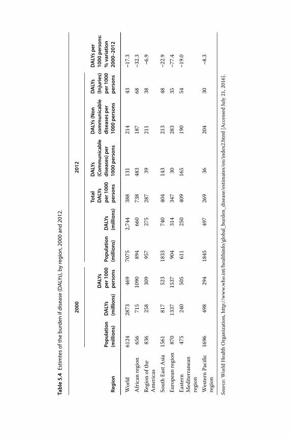
Tabl
e 5.
4 Es
timte
s of
the
burd
en if
dis
ease
(DA
LYs)
, by
regi
on, 2
000
and
2012
.
2000
2012
DA
LYs
per
1000
per
sons
: %
var
iatio
n 20
00–2
012
Regi
onPo
pula
tion
(mill
ions
)D
ALY
s (m
illio
ns)
DA
LYs
per 1
000
pers
ons
Popu
latio
n (m
illio
ns)
DA
LYs
(mill
ions
)
Tota
l D
ALY
s pe
r 100
0 pe
rson
s
DA
LYs
(Com
mun
icab
le
dise
ases
) per
10
00 p
erso
ns
DA
LYs
(Non
co
mm
unic
able
di
seas
es p
er
1000
per
sons
DA
LYs
(Inju
ries
) pe
r 100
0 pe
rson
s
Wor
ld61
2428
7346
970
752,
744
388
131
214
43−1
7.3
Afr
ican
regi
on65
671
510
9089
466
073
848
318
768
−32.
3Re
gion
of t
he
Am
eric
as83
625
830
995
727
528
739
211
38−6
.9
Sout
h Ea
st A
sia
1561
817
523
1833
740
404
143
213
48−2
2.9
Euro
pean
regi
on87
013
3715
3790
431
434
730
283
35−7
7.4
East
ern
Med
iterr
anea
n re
gion
475
240
505
611
250
409
165
190
54−1
9.0
Wes
tern
Pac
ific
regi
on16
9649
829
418
4549
726
936
204
30−8
.3
Sour
ce: W
orld
Hea
lth O
rgan
izat
ion,
http
://w
ww.
who
.int/
heal
thin
fo/g
loba
l_bu
rden
_dis
ease
/est
imat
es/e
n/in
dex2
.htm
l [A
cces
sed
July
21,
201
6].
The Populations of Poor Countries 181
we should return for a moment to Table 5.2. The average number of chil-dren per woman has declined by more than three, from 6.1 to 2.7, though China, which has reduced fertility to below‐replacement levels (from 6.1 to 1.6), is responsible for almost half of this decline. Fertility in the other large areas of the poor world differs widely: African fertility has under-gone a moderate decline from 6.6 to 4.3 children per woman, and birth control, south of the Sahara, is still rare;15 the change in southern central Asia has been larger still, with a reduction from 6.0 to 2.6, and this decline is due primarily to lower Indian fertility; southeastern Asia and Latin America (5.9 to 2.3) have registered larger declines. Taking into account the different scale of the demography of the poor world today, the c urrent situation resembles that of the western world at the beginning of the twentieth century when areas where fertility control was widely prac-ticed (like France) coexisted with others where “natural” fertility still prevailed (like certain areas of Mediterranean Europe or the northern and eastern peripheries of the continent).16
Fertility decline seems to have accelerated in recent years, an observa-tion supported by a comparison of the results of Demographic and Health Surveys (DHS) taken from the late 1980s to the present.17 Even in sub‐Saharan Africa fertility control seems to take hold although one would hope for a faster decline, given the very high rate of population growth. In some countries (Ghana, Kenya, Nigeria, Tanzania) the decline has stalled, raising worries as to future trends.18 Elsewhere, large c ountries such as Brazil, Iran, and Vietnam (beside China and South Korea that have fertility level below the lowest fertility of large European countries such as Russia, Germany, Italy, or Spain) are now well below the replacement level.
Explanation of these trends requires analysis of the principal compo-nents of human fertility, discussed in Chapter 1, Section 4. Recall that the average number of children per woman (TFR) is determined by a combi-nation of factors, predominantly biological, which determine natural fertility (birth intervals linked to the duration of breast‐feeding, waiting time linked primarily to the frequency of sexual relations, fetal mortal-ity); by marital patterns (age at marriage and percentage unmarried); and by the level of birth control.
I have already made reference to the fact that the “initial” fertility level of the poor countries – over six children per woman – was considerably higher than that of the West prior to the demographic transition (less than five). This is due primarily to higher levels of nuptiality: poor‐ country age at marriage (or the age at which a stable reproductive union is established) has traditionally been low, with almost no one remaining unmarried, unlike the situation in the West. The World Fertility Survey (WFS)19 revealed, for the late 1970s, an average age at first marriage of
A Concise History of World Population182
19.8 years in 12 African countries (from a minimum of 17.5 in Cameroon to a maximum of 23.9 in Tunisia); of 21 in 13 Asian and Pacific countries (from 16.3 in Bangladesh to 24.5 in the Philippines); and of 21.5 in 13 Latin American and Caribbean countries (from 19.2 in Jamaica to 23.2 in Peru). (These levels, considerably below the western average of about 24, are already 1 to 1.5 years above the levels of 15 years earlier.)20 In these same countries, and again according to the WFS, the percentage of unmarried women at the end of the reproductive period was barely 1 percent in Africa and Asia and 4 percent in Latin America (as com-pared to levels often over 10 percent in the West).21 The situation is in rapid motion, although with unequal speed, and the age of women at first union is increasing rapidly whenever women’s prerogatives are rein-forced in terms of education, wages and income, less discrimination, and less inequality within and outside the family.22
However, although the Malthusian check does reduce fertility, its effec-tiveness is limited. For example, in the absence of voluntary fertility con-trol, an increase in age at marriage from 18 to 23 (a radical change in nuptial behavior) will result in a reduction of the number of children per woman of 1.5–2. Clearly this reduction is too small to bring fertility down to levels compatible with moderate rates of population growth. Moreover, delayed marriage must translate into an effective delaying of women’s entry into motherhood and implies that reproduction be confined to within marriage. While this is true in Asia, where nonmarital fertility is practically negligible, it is not for Africa, Latin America, and the Caribbean, where reproduction outside marriage is common.
The decisive check to fertility, however, is its voluntary control. A simple measure of its “prevalence” is the percentage of women of reproductive age who, in a given period, use some methods of birth control. This p ercentage in turn can be broken down according to the method used (“traditional” and less‐efficient methods, like coitus interruptus or peri-odic abstinence – rhythm – or “modern,” more‐efficient methods, like the pill, IUDs, and sterilization). Contraceptive prevalence of about 70 percent and above indicates low levels of fertility like those found in the rich countries.23 The WFS (for 38 developing countries in the late 1970s) found levels of contraceptive prevalence of only 10 percent in Africa, 23 percent in Asia, and 40 percent in Latin America and the Caribbean. About three out of four of the women practicing some form of birth control used the so‐called “modern” methods.24 The countries investigated by the DHS between 2011 and 2014 show that contraceptive prevalence is still very low in Africa, remaining below 30 percent in countries like Nigeria, the Democratic Republic of Congo and Ethiopia, Africa’s giants. There is still a lot of ground to be covered, if we think that even in the poorest countries, like Cambodia (56 percent) and Bangladesh
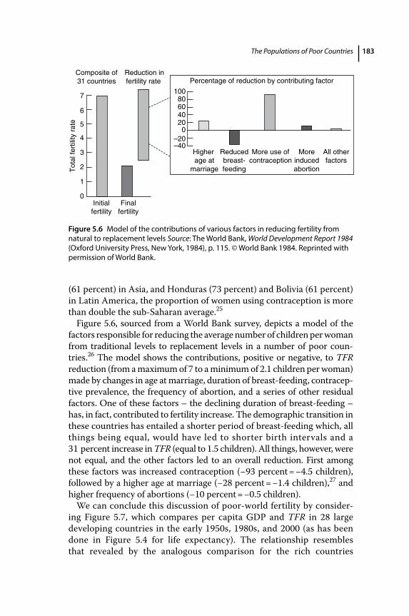
The Populations of Poor Countries 183
(61 percent) in Asia, and Honduras (73 percent) and Bolivia (61 percent) in Latin America, the proportion of women using contraception is more than double the sub‐Saharan average.25
Figure 5.6, sourced from a World Bank survey, depicts a model of the factors responsible for reducing the average number of children per woman from traditional levels to replacement levels in a number of poor coun-tries.26 The model shows the contributions, positive or negative, to TFR reduction (from a maximum of 7 to a minimum of 2.1 children per woman) made by changes in age at marriage, duration of breast‐feeding, contracep-tive prevalence, the frequency of abortion, and a series of other residual factors. One of these factors – the declining duration of breast‐feeding – has, in fact, contributed to fertility increase. The demographic transition in these countries has entailed a shorter period of breast‐feeding which, all things being equal, would have led to shorter birth intervals and a 31 percent increase in TFR (equal to 1.5 children). All things, however, were not equal, and the other factors led to an overall reduction. First among these factors was increased contraception (−93 percent = −4.5 children), followed by a higher age at marriage (−28 percent = −1.4 children),27 and higher frequency of abortions (−10 percent = −0.5 children).
We can conclude this discussion of poor‐world fertility by consider-ing Figure 5.7, which compares per capita GDP and TFR in 28 large developing countries in the early 1950s, 1980s, and 2000 (as has been done in Figure 5.4 for life expectancy). The relationship resembles that revealed by the analogous comparison for the rich countries
Initialfertility
0
1
2
3
4
Tot
al fe
rtili
ty r
ate 5
6
7
Finalfertility
Higher age at
marriage
–40–20
020406080
100
Composite of31 countries Percentage of reduction by contributing factor
Reducedbreast-feeding
More use ofcontraception
Moreinducedabortion
All otherfactors
Reduction infertility rate
Figure 5.6 Model of the contributions of various factors in reducing fertility from natural to replacement levels Source: The World Bank, World Development Report 1984 (Oxford University Press, New York, 1984), p. 115. © World Bank 1984. Reprinted with permission of World Bank.
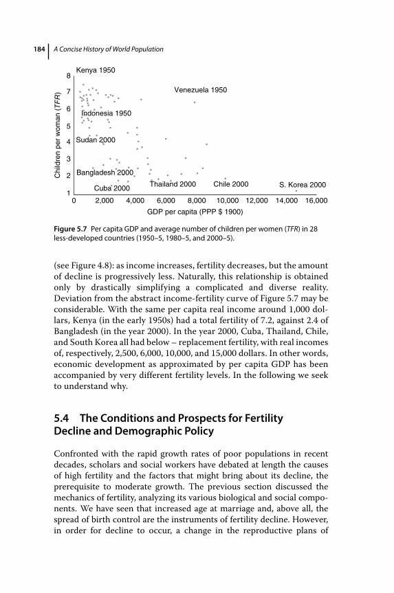
A Concise History of World Population184
(see Figure 4.8): as income increases, fertility decreases, but the amount of decline is progressively less. Naturally, this relationship is obtained only by drastically simplifying a complicated and diverse reality. Deviation from the abstract income‐fertility curve of Figure 5.7 may be considerable. With the same per capita real income around 1,000 dol-lars, Kenya (in the early 1950s) had a total fertility of 7.2, against 2.4 of Bangladesh (in the year 2000). In the year 2000, Cuba, Thailand, Chile, and South Korea all had below – replacement fertility, with real incomes of, respectively, 2,500, 6,000, 10,000, and 15,000 dollars. In other words, economic development as approximated by per capita GDP has been accompanied by very different fertility levels. In the following we seek to understand why.
5.4 The Conditions and Prospects for Fertility Decline and Demographic Policy
Confronted with the rapid growth rates of poor populations in recent decades, scholars and social workers have debated at length the causes of high fertility and the factors that might bring about its decline, the prerequisite to moderate growth. The previous section discussed the mechanics of fertility, analyzing its various biological and social compo-nents. We have seen that increased age at marriage and, above all, the spread of birth control are the instruments of fertility decline. However, in order for decline to occur, a change in the reproductive plans of
Venezuela 1950
Kenya 1950
Indonesia 1950
Sudan 2000
Bangladesh 2000
Cuba 20001
2
3
4
5
Chi
ldre
n pe
r w
oman
(TF
R)
6
7
8
0 2,000 4,000 6,000 8,000
GDP per capita (PPP $ 1900)
10,000 12,000 14,000 16,000
Thailand 2000 Chile 2000 S. Korea 2000
Figure 5.7 Per capita GDP and average number of children per women (TFR) in 28 less‐developed countries (1950–5, 1980–5, and 2000–5).
The Populations of Poor Countries 185
c ouples is necessary. We must therefore understand what determines these plans and what can be done to change them. To borrow the econo-mist’s terminology we must understand what determines the “demand” for children on the part of parents – still high in the poor countries – and what the factors are that might change it.28
In the first place, we may take for granted that preservation and sur-vival (of the individual, the family group, or the collectivity to which they belong) are innate values of the human species, just as they are for other animal species. Fertility therefore must compensate for mortality; when the latter is high, the former must be so as well. From this point of view, five or six children per woman are compatible with normal pretransition mortality levels. Often the risk of having no surviving heir induces c ouples to have many children as a sort of insurance, with the result that aggregate fertility is higher than general mortality. As stated above, mortality decline is a necessary prerequisite to fertility decline.
In many poor countries mortality, but not fertility, has declined consid-erably. Why does fertility remain high? Why has the “demand” for c hildren by parents not slackened? First, the cost of raising children remains low. In rural areas and under certain conditions, children may constitute a net gain for their parents. The work performed by children and adolescents may offset the costs sustained by the family, which in any case are low in a poor economy.29 Second, in many social contexts p arents consider children a guarantee of economic and material assistance, not to mention affection, in old age. Studies in Indonesia, Korea, Thailand, Turkey, and the Philippines reveal that 80 to 90 percent of parents inter-viewed count on receiving economic assistance from their children in old age.30 And in any case, it is natural to depend upon help from one’s c hildren in the event of great misfortune.31 Third, cultural context often demands a large number of children: as an affirmation of the family, as a guarantee of generational continuation, or as the expression of deep‐rooted religious principles. Finally, ignorance of birth control methods, unavailability of contraceptives, and inadequate medical and health s ervices contribute to inadequate fertility control or increased recourse to abortion. Legislation controlling the spread of contraceptives can r einforce these barriers to fertility decline.
If these are the causes of high fertility, then it is necessarily by means of their modification that the birth rate might decline. Above all, mortality must decline. Figure 5.2 (in which fertility and mortality are compared) indicates that almost all countries with a life expectancy over 65 have a relatively low TFR, the result of a certain degree of fertility control inde-pendent of socioeconomic conditions.
The increasing “relative cost” of child rearing also appears to be a fac-tor in fertility decline. This increase may, for example, come about as the
A Concise History of World Population186
result of expanded female education, so that women are less willing to give up the possibility of wage‐earning employment in favor of house-work and raising children. Other factors might include compulsory childhood schooling, which delays the beginning of a child’s work life, or a general increase in well‐being and the attendant requirements for greater investments in children. The creation of institutional mechanisms of social protection reduces the need of aging parents for support from their children, and so another incentive to high fertility is undermined. Other elements that tend to hasten fertility decline include the elimina-tion of legislative obstacles to birth control, a policy actively supporting family planning, the spread of contraceptive knowledge and techniques, and the fact they are affordable and psychologically acceptable.
None of the above factors can, on its own, bring about the transition from high to low fertility levels, and the proper combination of factors is difficult to determine, since it depends upon many characteristics of the society in question. The elements discussed entail improvements in medical and health services, economic development, and social change (changes in values, empowerment for women, secularization of behavior) – essentially all the aspects of societal development. No one aspect will effect change, and each country will have to find the appropriate mix.
Nonetheless, certain forms of intervention are simpler or more con-tained than others and so are more probable instruments of policy. Since the 1950s, for example, family planning has been a preferred approach and, generally speaking, it is unlikely that fertility decline will occur without an adequate network of these services.32 Today, the political acceptability of this sort of intervention is taken for granted, but this was not always the case. In the 1950s and 1960s, family‐planning programs – often naively and even clumsily introduced – were opposed in much of the poor world. In those countries embracing a socialist political system or ideology, for example, it was claimed that economic development would spontaneously regulate fertility. In others, ruling nationalists viewed birth control policies as an attack on the numerical strengthening of the nation, while these poli-cies were opposed on moral grounds in countries where religious funda-mentalism played an important role. The support given by rich countries – especially the United States – to these programs, often with dubious motivation, was considered a subtle form of capitalist imperial-ism. However, in 1974, at the United Nations World Population Conference in Bucharest33 (a conference restricted to official national delegations), China, Algeria, Brazil, and Argentina headed a large group of nations opposed to policies aimed at lowering population growth rates. On the other hand, many Asian countries, especially those of the Indian subconti-nent, were in favor of such policies. A memorable slogan from that confer-ence claimed that “development is the best contraceptive.” In Mexico City
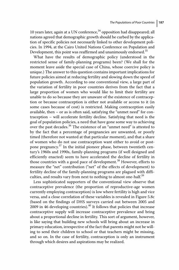
The Populations of Poor Countries 187
10 years later, again at a UN conference,34 opposition had disappeared; all nations agreed that demographic growth should be curbed by the applica-tion of specific policies not necessarily linked to other development poli-cies. In 1994, at the Cairo United Nations Conference on Population and Development, this point was reaffirmed and unanimously endorsed.35
What have the results of demographic policy (understood in the restricted sense of family‐planning programs) been? (We shall for the moment leave aside the special case of China, whose coercive policy is unique.) The answer to this question contains important implications for future policies aimed at reducing fertility and slowing down the speed of population growth. According to one conventional view, a large part of the variation of fertility in poor countries derives from the fact that a large proportion of women who would like to limit their fertility are unable to do so because they are unaware of the existence of contracep-tion or because contraception is either not available or access to it (in some cases because of cost) is restricted. Making contraception easily available, then – or as is often said, satisfying the “unmet need” for con-traception – will accelerate fertility decline. Satisfying that need is the goal of population policies, a need that have gone some way to achieving over the past decades.36 The existence of an “unmet need” is attested to by the fact that a percentage of pregnancies are unwanted, or poorly timed (therefore not wanted at that particular moment), and that a share of women who do not use contraception want either to avoid or post-pone pregnancy.37 In the initial pioneer phase, between twentieth cen-tury’s 1960s and 1990s, family‐planning programs (if well designed and efficiently enacted) seem to have accelerated the decline of fertility in those countries with a good pace of development.38 However, efforts to measure the “net” contribution (“net” of the effects of development) to fertility decline of the family‐planning programs are plagued with diffi-culties, and results vary from next to nothing to almost one‐half.39
Less sophisticated supporters of the conventional view observe that contraceptive prevalence (the proportion of reproductive‐age women currently employing contraception) is low where fertility is high and vice versa, and a close correlation of these variables is revealed in Figure 5.8c (based on the findings of DHS surveys carried out between 2005 and 2009 in 46 developing countries).40 It follows that policies that increase contraceptive supply will increase contraceptive prevalence and bring about a proportional decline in fertility. This sort of argument, however, is like saying that building new schools will bring about an increase in primary education, irrespective of the fact that parents might not be will-ing to send their children to school or that teachers might be missing, and so on. In the case of fertility, contraception is only an instrument through which desires and aspirations may be realized.
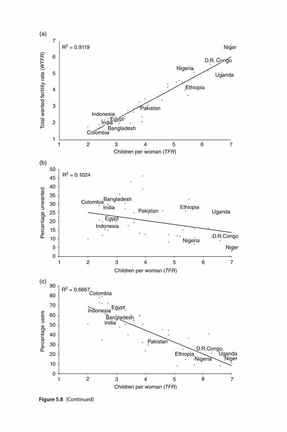
11
2
2Children per woman (TFR)
Children per woman (TFR)
Children per woman (TFR)
3
3
4
4
5
5
6
R2 = 0.9119
R2 = 0.1024
R2 = 0.6667
Tota
l wan
ted
fert
ility
rat
e (W
TFR
)P
erce
ntag
e un
wan
ted
Per
cent
age
user
s
6
Niger
Niger
Niger
Uganda
Uganda
Uganda
D.R.Congo
D.R.Congo
Nigeria
Nigeria
Nigeria
Ethiopia
Ethiopia
Ethiopia
Pakistan
Pakistan
Pakistan
Indonesia
IndonesiaEgypt
Bangladesh
Bangladesh
IndiaColombia
Colombia
7
7
10
5
10
15
20
25
30
35
40
45
50(b)
(c)
(a)
2 3 4 5 6 7
10
10
20
30
40
50
60
70
80
90
2 3 4 5 6 7
EgyptIndia
IndonesiaEgypt
BangladeshIndia
Colombia
D.R. Congo
Figure 5.8 (Continued)
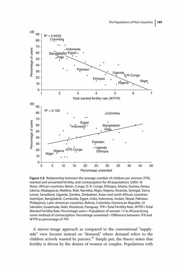
The Populations of Poor Countries 189
A mirror‐image approach as compared to the conventional “supply‐side” view focuses instead on “demand,” where demand refers to the c hildren actively wanted by parents.41 Simply put, the theory states that fertility is driven by the desires of women or couples. Populations with
Figure 5.8 Relationship between the average number of children per woman (TFR), wanted and unwanted fertility, and contraception for 40 populations (2005–9) Notes: African countries: Benin, Congo, D. R. Congo, Ethiopia, Ghana, Guinea, Kenya, Liberia, Madagascar, Maldive, Mali, Namibia, Niger, Nigeria, Rwanda, Senegal, Sierra Leone, Swaziland, Uganda, Zambia, Zimbabwe. Asian and north‐African countries: Azerbijan, Bangladesh, Cambodia, Egypt, India, Indonesia, Jordan, Nepal, Pakistan, Philippines. Latin American countries: Bolivia, Colombia, Dominican Republic, El Salvador, Guatemala, Haiti, Honduras, Paraguay. TFR = Total Fertility Rate. WTFR = Total Wanted Fertility Rate. Percentage users = Population of women 15 to 49 practicing some method of contraception. Percentage unwanted = Difference between TFR and WTFR as percentage of TFR.
10
10
20
30
40
50
60
70
80
90(d)
(e)
2 3 4 5 6 7
Total wanted fertility rate (WTFR)
R2 = 0.6532
R2 = 0.129
Per
cent
age
of u
sers
00
10
20
30
40
50
60
70
80
90
5 10 252015 3530 4540 50Percentage unwanted
Per
cent
age
of u
sers
Niger
UgandaD.R.Congo
NigeriaEthiopia
Pakistan
IndonesiaEgypt
India
Niger
UgandaD.R.CongoNigeria Ethiopia
Pakistan
IndonesiaEgypt
BangladeshIndia
Colombia
Colombia
Bangladesh
A Concise History of World Population190
high fertility, then, also have a high demand for children. Even if the supply of family‐planning services is high and they are efficiently run, they will be little used and fertility will remain high. This situation is particularly fre-quent in sub‐Saharan countries and among many Islamic populations. Conversely, low demand for children coincides with low fertility even in the absence of family‐planning programs. Indeed, in western countries fertility declined in the first two‐thirds of the twentieth century in spite of legislation hostile to family planning and a limited supply of contracep-tives (advertising contraceptives was illegal in many countries until the 1950s and 1960s). The level of fertility, then, is dictated by motivations, expectations, and desires. If these change, so will fertility. Figure 5.8 lends some support to this view. Indeed Figure 5.8c – as we have seen – shows the close inverse relation between fertility and contraceptive prevalence, but the same association can also be seen between wanted fertility and contraceptive prevalence (Figure 5.8d).42 The close similarity of the two figures implies a very close association between actual and wanted fertil-ity, as is indeed shown by Figure 5.8a. In other words, variation in actual fertility is almost completely explained by variation in wanted fertility. When fertility is high, wanted fertility is also high. Figures 5.8b and 5.8e are even more interesting. In Figure 5.8b, actual fertility is compared to the proportion of fertility that is unwanted.43 As we can see, there is no correlation between the two variables: indeed, with the decline of fertility toward small family norms there is no attendant decline of unwanted f ertility. On the contrary, unwanted fertility seems to increase in the inter-mediate stages of the fertility transition. A similar observation can be made regarding Figure 5.8e, where the proportion of unwanted fertility is compared to the prevalence of contraception. One would think that increased prevalence of contraception should reduce unwanted fertility, but such is not the case. A study suggests instead that the variation of fertility across countries (holding desires constant) is explained only in minimal part (1 or 2 percent) by variation in contraceptive prevalence.44
To sum up: (1) fertility is driven by motivations and desires; (2) contra-ception is a necessary technical instrument for controlling fertility, but its availability – other factors being equal – has little impact on fertility and does not reduce unwanted fertility; (3) policies directed to lower fertility must be “demand‐oriented,” trying to influence the factors that determine the propensities, desires, and motivations of couples.
This debate has been useful in providing better guidelines for policies. It is clear that small family norms, well‐rooted in society, cannot be brought about by family‐planning programs alone, no matter how well conceived and aggressive they might be. Paul Demeny has identified four factors as particularly important in determining the fertility transition: (1) the direct cost parents must incur in raising and educating their
The Populations of Poor Countries 191
children; (2) the opportunity costs of children to parents (or the earnings that a couple – in general the woman – forgoes because of children); (3) the contribution that children’s labor makes to the income of the fam-ily; (4) the contribution of children to parents’ economic security in old age relative to other forms of security.45 Therefore, those policies that tend to favor the responsibility of parents in raising children, including bearing part of the cost of education and health; that encourage women to enter the labor force; that enforce compulsory education of children; that make child labor illegal; and that develop old‐age private or public insurance schemes are conducive to fertility decline. The combination of these policies with well‐balanced programs for family planning and reproductive health – which increase access to contraception, reduce its cost, and compress recourse to abortion – may accelerate a smooth transi-tion to low fertility.
5.5 India and China
By the mid‐1980s almost all the governments of the world officially sup-ported family planning to some degree; the United Nations announced that this was the case for 127 countries comprising 94 percent of the world’s population.46 However, behind these encouraging figures are both successes and failures, as well as combinations of the two. The cases of India and China are representative and merit attention if only by virtue of the demographic dimensions of both countries: together they account for about half the total population of developing countries.
Demographic data for the two countries are listed in Table 5.5 and require little commentary. Between the early 1950s and 2010–15 Chinese fertility was reduced by three‐quarters, while that of India has declined by 60 percent; Chinese life expectancy at birth, at the same level as India’s in the 1960s, is now 8 years longer. Today, Chinese fertility is below replacement level, and if it remains there the population will eventually decline (and according to the latest United Nations projections, this could take place in the late 2020s). By contrast, Indian fertility – 1 child per woman more than China – ensures continued rapid population growth.
In order to understand these great differences we must consider the demographic policies adopted by these two countries and their results. The Indian government has pursued slower demographic growth since 1952. The first two 5‐year plans (1951–6 and 1956–61) called for the creation of family planning centers; the fifth plan (1971–6) called for a crude birth rate of 25 per 1,000 by 1984 (clearly a goal that was not met, as the 1980–5 birth rate was 10 points higher).47 Accomplishments have
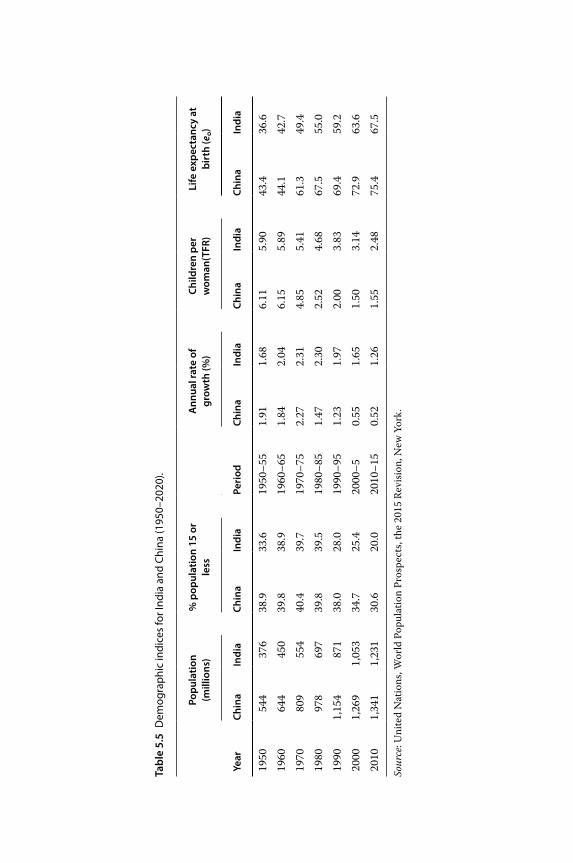
Tabl
e 5.
5 D
emog
raph
ic in
dice
s fo
r Ind
ia a
nd C
hina
(195
0–20
20).
Popu
latio
n (m
illio
ns)
% p
opul
atio
n 15
or
less
Ann
ual r
ate
of
grow
th (%
)Ch
ildre
n pe
r w
oman
(TFR
)Li
fe e
xpec
tanc
y at
bi
rth
(eo)
Year
Chin
aIn
dia
Chin
aIn
dia
Peri
odCh
ina
Indi
aCh
ina
Indi
aCh
ina
Indi
a
1950
544
376
38.9
33.6
1950
–55
1.91
1.68
6.11
5.90
43.4
36.6
1960
644
450
39.8
38.9
1960
–65
1.84
2.04
6.15
5.89
44.1
42.7
1970
809
554
40.4
39.7
1970
–75
2.27
2.31
4.85
5.41
61.3
49.4
1980
978
697
39.8
39.5
1980
–85
1.47
2.30
2.52
4.68
67.5
55.0
1990
1,15
487
138
.028
.019
90–9
51.
231.
972.
003.
8369
.459
.220
001,
269
1,05
334
.725
.420
00–5
0.55
1.65
1.50
3.14
72.9
63.6
2010
1,34
11,
231
30.6
20.0
2010
–15
0.52
1.26
1.55
2.48
75.4
67.5
Sour
ce: U
nite
d N
atio
ns, W
orld
Pop
ulat
ion
Pros
pect
s, th
e 20
15 R
evis
ion,
New
Yor
k.
The Populations of Poor Countries 193
been few and fertility decline minimal: in 1970 the percentage of couples (woman of reproductive age) using birth control was very low (14 percent). For both males and females the most frequent method was sterilization.48 Success has been limited to a few states, the upper classes, and the urban population. Confronted with these poor results – caused by insufficient investment but also discontinuities in, and the difficulty of, administer-ing the program in a country characterized by a variety of languages, religions, and customs – Indira Gandhi’s government decided in 1976 to speed up the program. With the declaration of April 16, 1976, the g overnment implemented a series of measures (including strengthening of the existing program and increased financial incentives for the partici-pants) and encouraged the state legislatures to pass laws making sterili-zation obligatory after the birth of the third child (only the state of Maharastra passed such a law, and it was not enforced).49 This coercive line inspired violent protests that were among the causes of the defeat of Gandhi’s Congress Party in the March, 1977 elections.50 As a result, the Indian program suffered a notable setback. Indira Gandhi’s return to power in 1980 and the unexpected results of the 1981 census (which revealed a population considerably larger than expected) led to renewal of the demographic policy. The seventh 5‐year plan of 1986–90 called for the achievement of replacement fertility by the year 2000. This was an unrealistic goal because it would have required a fertility decline similar to that experienced in China during the 1970s under exceptional and perhaps nonrepeatable conditions; indeed, by 2000, fertility was still 50 percent above replacement. The Indian plan called for greater invest-ment in the family‐planning program; increased financial incentives for its participants; a big increase in sterilization and more widespread use of the IUD, as well as other forms of birth control; and combining family planning services with maternal and infant services.51
Despite official support (for 30 years) of family planning, the gov-ernment of India has not been able to organize a birth control program that regularly provides adequately staffed services to most of the population. At different times the responsible central agency … has promoted different methods of contraception and tried different organizational approaches. At first, when modern contraceptives were not widely used anywhere in the world, there was a hope, soon disappointed, that periodic continence (the rhythm method) would reduce the birth rate in India, where it seemed to conform so well with Gandhian principles. Later there was primary reliance on the intrauterine device, but the health and family planning network never developed the capacity for skillful insertion, proper monitoring, and adequate counseling to counter
A Concise History of World Population194
exaggerated reports about the dangers of the device, to reassure patients about the side effects, or overall to obtain sustained high rates of insertion and retention. For various reasons, oral c ontraceptives have never been authorized for use in India.52
This was the harsh judgment of Ansley Coale, an expert on the Indian demographic situation. The only aspect of the program that enjoyed a degree of success was sterilization, the frequency of which increased d ramatically in 1976–7 (8 million sterilizations in 2 years as compared to an average of 2 million per year in the preceding decade). After Gandhi’s defeat, however, the sterilization program came to a sudden halt and has only shown signs of recovery in recent years.
The 1980s should have signaled a new strategy, concentrating not only on family planning but also on those aspects of social and economic development that favor fertility decline: increasing age at marriage, r aising the status of women, improving female literacy, enhancing child survival, alleviating poverty, and providing security for old age.53 These good intentions, however, have had little effect. In spite of increased resources, the 1980s witnessed “a steep decline in the quality of family planning and public health practice” due to the increasing role played by bureaucrats as opposed to specialists.54 At the end of his term as prime minister, Rajiv Gandhi issued sharp criticism of population policy failure in India, citing excessive bureaucratic centralization of the program, which allows little flexibility in a country characterized by vastly differing needs.55 In recent years, the government seems to have adopted a more diversified approach: couples are provided with information on a broad range of family planning methods, and the family planning targets set in various districts have been eliminated in order to dispel fears of coercion. A survey of 2005–6 (National Family Health Survey) estimated a total fertility rate of 2.7 (against 2.9 of the preceding survey of 1998–9 and 3.4 of the one carried out in 1992–3); 56 percent of women used contracep-tion, mainly sterilization; about four‐fifths of all contraceptives were obtained from public sources. New steps, then, have been made in spite of the uncertain role of government actions. In the urban population fertility is now at replacement level, while the populations of the south of the country are below replacement. But in the populous states of Uttar Pradesh, Madhya Pradesh, Bihar, and Rajasthan, with a total of 450 mil-lion inhabitants, total fertility is still above three and the diffusion of control is slow. With a population that at the 2011 Census amounted to 1.210 billion, with a 1.6 percent growth rate that will result in India being the most populous country of the world in 2022, the Indian government is wary of the nation’s demographic future. A National Population Policy was launched in 2000 with the objective of stabilizing the population by
The Populations of Poor Countries 195
2045 (but for the latest United Nations projections this will happen in 2068, with a population of 1.754 billion). The government, aware of the fierce popular opposition to coercive policies, affirms that the new popu-lation policy will refuse coercion and force and will be based on “informed consent and democratic principles.”56 The policy seeks a closer involve-ment of local authorities; participation of men in family planning p rograms; incentives in order to raise the age at marriage; incentives to couples having no more than two children. More precisely, these are aimed at couples living in poverty who postpone marriage after the legal age of 21 and have no more than two children, or spouses who undergo sterilization after the birth of the second child. There is, however, consid-erable criticism concerning some aspects of the policy, particularly for the government‐sponsored family planning camps where women can undergo sterilization for monetary gain. Convincing poorly educated women in remote communities to use contraceptives is more expensive than the mass‐sterilization campaigns and incentives are often seen as forms of indirect coercion. Finally, there is a very worrying aspect of the recent demographic development of the country. The male to female ratio among the newborn is rapidly increasing in many states, and p articularly in those with higher standards of living, such as Haryana, Punjab, and Gujarat. This is a widespread phenomenon in China and Southeast Asia, due to selective abortion induced by couples’ preferences for male children. In many regions of the country, the worsening of this dramatic distortion generates a growing imbalance in the gender compo-sition of the population. This will translate into the exclusion from m arriage of a considerable proportion of men, particularly among the poorest strata of society, with complex negative consequences. Various measures are being tried, in India and elsewhere, in order to counter this dangerous trend.
The history of government family‐planning programs in China differs considerably from that of India.57 In 1949 Mao declared: “China’s vast population should be viewed as a positive asset. Even if it should multiply many times, it will be fully able to resolve the problems created by this growth. The solution lies in production … Revolution and production can resolve the problem of feeding the population.”58 However, as the revolution was consolidated and the results of the 1953 census became known, concern over the population problem began to emerge. At the Eighth Party Congress in 1956 Zhou En‐lai’s speech included these remarks: “We all agree on the desirability of adopting measures favoring birth control, both for the protection of women and children and to ensure that the younger generations are brought up and educated in such a way as to guarantee national health and prosperity.”59 This first birth control program required the creation of an assistance network, the
A Concise History of World Population196
production of contraceptives, and a plan to encourage the population to use these birth control services and devices. However, demographic pru-dence was not in keeping with the ambitious socioeconomic program of 1958/9 – the Great Leap Forward – and the attendant blind faith in gigantic productivity goals. As a result the program came to a sudden halt but, after the failure of the Great Leap Forward, poor harvests, fam-ine, and the high mortality of 1959–61, a second campaign was launched with the creation of a Department of Family Planning. This second cam-paign that, among other things, introduced the IUD and advocated later marriage, was essentially suspended during the Cultural Revolution. It was only with the return to normality in 1971 that the third campaign began. This was based on three principles: later marriage, longer birth intervals, and fewer children. Later marriage meant, for women, 23 years of age in rural areas and 25 years of age in the city; longer intervals meant 4 years between the first and second child; and fewer children meant no more than two children in the city or three in the country. In 1977 the latter limit was lowered to two for both city and country. The unquestioned success of this program in the 1970s was due to a system of birth quotas:
According to this system, the Chinese government began to estab-lish annual numerical objectives for the natural rate of population increase in each province … Provincial authorities and prefects, in turn, translated their assigned rate into a birth quota, distributing this quota among the prefectures and counties under their juris-diction. This process continued on down until it reached the work team or its urban equivalent.60
Within these groups, couples planning to have children met with group leaders to determine which were entitled to have a child the following year. About half of the couples practicing birth control used an IUD, about one‐third used sterilization, and the remainder chose a variety of other methods, including a considerable proportion using steroids.61 Abortion also became widespread and easily obtainable, free of charge, and did not require the husband’s consent.
After Mao’s death and the defeat of the Gang of Four, demographic objectives became both more explicit and more ambitious. During the second session of the Fifth National People’s Assembly in 1979, Hua Guofeng affirmed that a large reduction in demographic growth was one of the essential conditions for the success of the “four modernizations” (of agriculture, defense, industry, and science and technology). Initially, the aim was to reduce the rate of natural increase to 0.5 percent in 1985 and zero in the year 2000. In September, 1980, Hua updated these objec-tives, the new goal being to not exceed 1.2 billion in 2000. In order to
The Populations of Poor Countries 197
accomplish this goal a birth limit of one child per couple was established in 1979, with exceptions for ethnic minorities, border areas, and couples in special situations. A series of incentives and disincentives has been introduced in order to meet this difficult goal. The primary tool has been the one‐child certificate, issued by local authorities, which guarantees a series of benefits for couples and their children in exchange for the com-mitment not to have more than one child. The benefits include wage and pension increases, larger dwellings, free medical care, and priority for the child in school. Couples who refuse to cooperate and give birth to a s econd, or worse a third, child are penalized in the form of wage cuts, revocation of privileges, and other disincentives.62
The Chinese one‐child policy has been pursued with varying intensity. Until 1983, pressure increased as coercive, even brutal, methods were implemented on a vast scale. The resulting protests and discontent, how-ever, led to a period of uncertainty. On the one hand, recognition of the growing number of women of reproductive age born during the period of fertility increase that followed the catastrophic Great Leap Forward (between 1983 and 1993 the number of women aged 21 to 30 increased from 80 to 125 million) argues for maintaining the policy;63 on the other hand, the protest and resistance of a population denied one of the most basic of human rights urges its relaxation. The 1990 census counted 1.134 billion Chinese and revealed that the official goals could not be easily realized. Until 1985, government policy continued to target a population not over 1.2 billion by the year 2000, but this formula had later been made more elastic, calling for “about 1.2 billion,” which in practice meant that the ceiling had been lifted to 1.25 billion. This limit was also officially revised to 1.3 billion, above the 1.265 counted by the Census in the same year.64 The discontent of the population, denied one fundamental human right, was an argument for relaxing the coercive policy. The 1980s were indeed characterized by several examples of the relaxation of the policy: the progressive extension of the right of rural couples to have a second child when the firstborn is a girl, or permission granted on special, probably discretionary, grounds, or because the f amily lived in a remote area or had special characteristics.65 Fertility decline stopped in the first part of the 1980s and fertility even increased between 1985 and 1987 (TFR grew from 2.3 to 2.5). The dismantling of the socialist collectives, which were an essential tool of family planning policies, “led to an erosion of cadre power and a breakdown of the system of economic incentives and disincentives on which policy enforcement had been largely based.”66 Moreover, the process of economic liberali-zation and the general attenuation of public control over individual behavior increased the obstacles to full implementation of the policy. Nonetheless, at the beginning of the 1990s the Chinese leadership
A Concise History of World Population198
renewed its commitment to the one‐child policy, leaving the regulations intact and strengthening their implementation: a nationwide fertility sur-vey put total fertility at 1.9 for 1992, well below the average level of the 1980s. Apparently this new party‐led drive enjoyed success, reinforcing commitment to family planning at all levels and responsibility systems, strengthening economic incentives and penalties, introducing old‐age insurance schemes, and so on.67 Continuing rapid economic growth and associated social change have also influenced reproductive norms and values, thus facilitating the task of policymakers. Many provinces now offer exemptions to the one‐child commitment to young people who have no siblings. When two of these young people marry, they will be allowed to have two children. According to the current legislation, the one‐child policy is strictly enforced among couples holding an on‐agricultural household registration status nationwide plus all couples in two large provinces (Sichuan and Jiangsu), representing 35 percent of the total population. The policy allowing couples whose first child is a girl to have a second child applies to 54 percent of the population. The residual 11 percent is made up of peripheral populations composed of ethnic minorities that are allowed to have two and even three children. If these rules were severely enforced, the TFR of the Chinese population would be 1.5. That the current policy should be abandoned or phased out has been a widespread opinion for years, and for three major considerations. The first was that low‐fertility preferences had become well rooted in the couples’ behaviors and that, at the same time, coercive policies were at risk of being on a collision course with the aspirations and the modes of life of the young generations. It had been observed that a high proportion of couples living in rural areas and who were allowed to have a second child renounced this possibility. Various studies demonstrated that aban-doning the one‐child policy would have had a small effect on the aggre-gate fertility of the country. The second consideration was that the combination of the one‐child policy and of the deeply rooted aspiration to have a male heir had strongly altered the sex ratio at birth, that had increased to 120 (against a natural level of 105–6; it was 108 in 1982). This was, and is still today, the consequence of sex‐selective abortion and of the higher infant and child mortality of baby girls in comparison with the boys of the same age, because of various forms of child neglect and discrimination. It is true that a similar distortion is typical of other coun-tries of Southeast Asia (and of India) that do not have a one‐child policy; nevertheless, in China, the distortion has reached record levels. The third element was that very low fertility alters the age structure, acceler-ates the aging process, and weakens the support system of the older population. There will be an acceleration of the aging process in the sec-ond and third decades of the twenty‐first century when the numerous
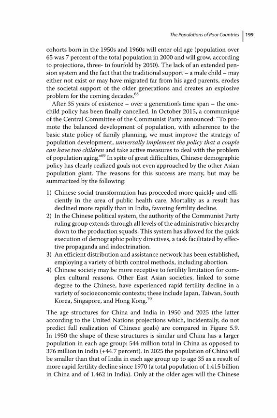
The Populations of Poor Countries 199
cohorts born in the 1950s and 1960s will enter old age (population over 65 was 7 percent of the total population in 2000 and will grow, according to projections, three‐ to fourfold by 2050). The lack of an extended pen-sion system and the fact that the traditional support – a male child – may either not exist or may have migrated far from his aged parents, erodes the societal support of the older generations and creates an explosive problem for the coming decades.68
After 35 years of existence – over a generation’s time span – the one‐child policy has been finally cancelled. In October 2015, a communiqué of the Central Committee of the Communist Party announced: “To pro-mote the balanced development of population, with adherence to the basic state policy of family planning, we must improve the strategy of population development, universally implement the policy that a couple can have two children and take active measures to deal with the problem of population aging.”69 In spite of great difficulties, Chinese demographic policy has clearly realized goals not even approached by the other Asian population giant. The reasons for this success are many, but may be s ummarized by the following:
1) Chinese social transformation has proceeded more quickly and effi-ciently in the area of public health care. Mortality as a result has declined more rapidly than in India, favoring fertility decline.
2) In the Chinese political system, the authority of the Communist Party ruling group extends through all levels of the administrative hierarchy down to the production squads. This system has allowed for the quick execution of demographic policy directives, a task facilitated by effec-tive propaganda and indoctrination.
3) An efficient distribution and assistance network has been established, employing a variety of birth control methods, including abortion.
4) Chinese society may be more receptive to fertility limitation for com-plex cultural reasons. Other East Asian societies, linked to some degree to the Chinese, have experienced rapid fertility decline in a variety of socioeconomic contexts; these include Japan, Taiwan, South Korea, Singapore, and Hong Kong.70
The age structures for China and India in 1950 and 2025 (the latter according to the United Nations projections which, incidentally, do not predict full realization of Chinese goals) are compared in Figure 5.9. In 1950 the shape of these structures is similar and China has a larger population in each age group: 544 million total in China as opposed to 376 million in India (+44.7 percent). In 2025 the population of China will be smaller than that of India in each age group up to age 35 as a result of more rapid fertility decline since 1970 (a total population of 1.415 billion in China and of 1.462 in India). Only at the older ages will the Chinese
A Concise History of World Population200
0
0–45–9
10–1415–1920–2425–2930–3435–3940–4445–4950–5455–5960–6465–6970–74
80+(a)
China 1950India 195075–79
10 20 30Population (millions)
40 50 60 70 80
0
0–45–9
10–1415–1920–2425–2930–3435–3940–4445–4950–5455–5960–6465–6970–74
80+(b)
China 2025India 202575–79
20Population (millions)
40 60 120100 14080
Figure 5.9 Age structure in: (a) China and India (1950); (b) China and India (extrapolated for 2025).
The Populations of Poor Countries 201
population be much greater than that of India. Between 1950 and 2025 the population of India will almost quadruple, while that of China will increase by a factor of 2.6, and in 2022 India will have surpassed China in demographic dimensions.
It is too soon to make an historical evaluation of the demographic paths undertaken by the two Asian giants. The rapid deceleration of demographic growth in China has probably made a relevant contribution to the spectacular economic development since the 1970s, but the coun-try will have to be ready to absorb the shock of rapid aging in the coming decades as well as the political heritage of a coercive regime. On the other hand, India’s sustained population growth has probably been an obstacle to the modernization of the country and worsened many social problems, although it has not impeded the acceleration of economic growth and may spare the country the shock of violent changes in the age structure. Which of the two countries has followed a better course is a matter of debate, but this must also include – beside the demographic factor –complex ethical, political, and economic considerations.
5.6 Fertilia and Sterilia
In the tropical region of a large continent lie the two bordering lands of Fertilia and Sterilia, which have in common a primarily agricultural economy situated in the more temperate highlands. Sterilia has an outlet on the sea where its principal city is found. It has for centuries been a center of maritime commerce and trades with countries near and far, including a former colonial power. Sterilia’s population is, espe-cially in the coastal region, ethnically mixed as a result of the several currents of immigration that have peopled its shores. Fertilia, on the other hand, landlocked and extending to the interior of the continent, is characterized by ethnic homogeneity and a traditional culture. Politically it is dominated by an upper class of large landowners, and contact with the outside world is minimal. At the time of decoloniza-tion, which occurred contemporaneously in the two countries, the two populations were about the same size and had similar demographic characteristics: fertility was high and uncontrolled and mortality, though high by western standards, had nonetheless declined consid-erably thanks to the introduction of penicillin and the elimination of malaria by DDT spraying in the colonial era. As a result, both countries had high rates of growth, between 2 and 3 percent. Independence brought a coalition backed by the large landowners to power in Fertilia, while the merchant class gained hegemony in Sterilia. In addition to
A Concise History of World Population202
trade liberalization, one of the first political acts in Sterilia was the initiation of a vigorous family planning program, spread throughout the country by a system of internal communications and supported by foreign investment. A trained corps of personnel and a mobile network of consultants were quickly established. Other measures included liberalized abortion and sterilization, subsidies for contraceptives, and incentives for participation in the program. We shall probably never be able to determine whether this program was actually the cause of the profound changes in reproductive behavior that followed or else simply accelerated a transition already on the verge of initiation. In either case, fertility declined quickly, soon reaching replacement levels. By comparison, the more traditional government of Fertilia, influenced by fundamentalist religious groups and ruling a population little exposed to foreign contact and trade, only formally recognized the UN directive to respect the right of every couple to decide how many children it wanted. In spite of pressure from the ex‐colonial power, which provided considerable economic aid, no active family planning policy was initiated and, if anything, the government blocked similar programs advanced by private concerns. Birth control spread slowly and, 30 years after independence, the women of Fertilia bore on average two children more than those of Sterilia.
These two policies have affected the demographic growth and economic development of these countries very differently. The demographic consequences include divergent rates of growth and age structures. Equally populous at the time of independence (which, how-ever, was referred to as the Revolution in Sterilia), the ratio was 1.4:1 after 30 years (in favor of Fertilia naturally) and 2:1 after 60. In Sterilia, the population under the age of 15 accounted for 42 percent of the total at the time of the Revolution; after 30 years this figure had dropped to 27 and after 60 to 21 (at which time the growth rate was about zero). In Fertilia, on the other hand, the under‐15 proportion, equal to that of Sterilia at the time of independence (42 percent), declined more slowly, representing 38 p ercent of the total after 30 years and 30 percent after 60. At the latter date population growth was still running about 1.5 percent per year. By contrast, 60 years after the Revolution the pro-portion of the population over 65 in Sterilia (12 percent) was double that in Fertilia.
Differences in economic development have been equally significant. The high rate of growth in Fertilia has led to the quadrupling of the working‐age population with an attendant high level of agricultural underemployment. Strong currents of migration flow primarily toward the capital city, which has become a sprawling megalopolis crowded
The Populations of Poor Countries 203
with impoverished masses. Given the still large average family size, the average Fertilian’s small income goes almost entirely to obtaining the necessities of survival, leaving little for savings; this is to the detriment of investments, which only barely keep pace with population growth. The meager financial resources commanded by the government have been insufficient to expand infrastructure and services. In particular, the spread of education has been slow: in spite of the (slow) fertility decline, the school‐age population, between the ages of 5 and 15, has tripled in the 60 years considered. The combination of a slow rate of agricultural development and a high rate of urbanization has transformed the coun-try from an exporter of tropical products to a net importer of foodstuffs. Lack of investment has inhibited the development of its fragile manufac-turing industry, and the country has accumulated an enormous foreign debt. The growth of per capita income has been small, and the absolute n umber (if not the percentage) of the marginally poor and illiterate has increased dramatically.
Sterilia’s recent history differs substantially from that of Fertilia. Fertility limitation has ensured that, during the 60 years since the Revolution, the size of Sterilia’s school‐aged population has remained constant (as opposed to its tripling in Fertilia), which has enabled public monies to be used for considerable expansion and improvement of the education system. As a result, succeeding generations entering the labor market have been both smaller in number and better trained than in Fertilia. Labor force efficiency has increased rapidly, fueling development in both the traditional and modern sectors of the economy. Birth control has also meant smaller families and so more rapid emancipation of women and the possibility for personal savings of those resources no longer completely absorbed by basic needs. Greater savings have allowed investments to outpace demographic growth, making infrastructure modernization, greater agricultural production, and economic diversifi-cation possible. Moreover, changes in age structure have notably reduced the dependency ratio (the number of nonproductive members of s ociety – the old and the very young – per 100 productive members), and this too has favored economic development. This same process has p roceeded much more slowly in Fertilia. Lower levels of population increase and urbanization and above all improved agricultural produc-tivity have ensured that Sterilia remains a net exporter of foodstuffs, which has helped to finance the purchase of machinery for the develop-ment of the manufacturing industries. Per capita income has grown r apidly and, 60 years after the Revolution, Sterilia has half the population of Fertilia, a larger gross national product, and a standard of living envied by its neighbor.
A Concise History of World Population204
The preceding passage is an invention on the part of the author, but might be taken from the work of an historian attempting to describe and interpret the recent past of these two countries, also purely imaginary.71 Analyses of this sort have been frequent over the decades since World War II, during which the population growth rate of the developing coun-tries has risen dramatically, making demographic increase a major con-temporary concern. The contrast between Fertilia and Sterilia serves to illustrate the paths that the poorer nations have followed in recent dec-ades or might follow in the near future. However, the above analysis, while fairly convincing in its general line of reasoning, is less so for the basic assumptions it makes.
The first of these assumptions is that a rapidly growing population inevitably leads to diminishing returns from labor and other factors of production and so to that capital dilution which, all things being equal, increases poverty; according to this formula, the slower population growth of Sterilia is clearly an advantage. The second assumption is that smaller families lead to the creation of savings and so greater invest-ments, another point in Sterilia’s favor. The third is that slower popula-tion growth means greater workforce efficiency and therefore greater productivity. And according to the fourth, factors of scale related to demographic size are of little relevance and so do not benefit the more rapidly growing population. Similarly, population increase is assumed to have no positive effect on technological progress. In short, success at limiting demographic growth must be a determining factor of economic development. It should follow, then, that demographic growth and e conomic d evelopment since the 1960s or 1970s relate inversely to one another.
This final point, which sums up the previous ones, can be put to a first‐order test. It is a fairly crude test, analogous to that made in Chapter 4, Section 7 for the western countries, comparing population growth rates and per capita income in 28 poor countries.72 I need not repeat here the cautions I have already expressed at some length regard-ing this exercise.
Figure 5.10 plots the population growth rate against the per capita GDP growth rate for the period 1950–2000: there is a relatively close inverse association between the two variables. The connection between population growth and development is probably blurred by a series of factors that tend to cancel one another out. One is led to think that demographic growth has probably not been an insurmountable obstacle to increasing well‐being and that, for diverse and complicated reasons, those factors that seemed so clearly at work in Fertilia and Sterilia have in fact operated much less clearly in recent decades.73 I shall turn to this problem.
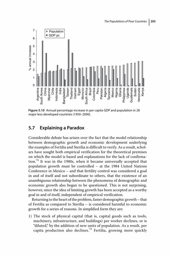
The Populations of Poor Countries 205
5.7 Explaining a Paradox
Considerable debate has arisen over the fact that the model relationship between demographic growth and economic development underlying the examples of Fertilia and Sterilia is difficult to verify. As a result, schol-ars have sought both empirical verification for the theoretical premises on which the model is based and explanations for the lack of confirma-tion.74 It was in the 1980s, when it became universally accepted that population growth must be controlled – at the 1984 United Nations Conference in Mexico – and that fertility control was considered a goal in and of itself and not subordinate to others, that the existence of an unambiguous relationship between the phenomena of demographic and economic growth also began to be questioned. This is not surprising, however, since the idea of limiting growth has been accepted as a worthy goal in and of itself, independent of empirical verification.
Returning to the heart of the problem, faster demographic growth – that of Fertilia as compared to Sterilia – is considered harmful to economic growth for a series of reasons. In simplified form they are:
1) The stock of physical capital (that is, capital goods such as tools, machinery, infrastructure, and buildings) per worker declines, or is “diluted,” by the addition of new units of population. As a result, per capita production also declines.75 Fertilia, growing more quickly
0
1
% a
nnua
l inc
reas
e
Arg
entin
a
Chi
naM
yanm
arC
hile
Indo
nesi
aIn
dia
Ban
glad
esh
Taiw
anT
haila
ndV
ietn
amE
gypt
Mor
occo
Sou
th A
fric
aB
razi
lC
olom
bia
Per
uP
akis
tan
Alg
eria
Tanz
ania
Mex
ico
Nig
eria
Gha
naP
hilip
pine
sU
gand
aG
uate
mal
aS
udan
Ven
ezue
laK
enya
Sou
th K
orea
2
3
4
5
6
7 PopulationGDP pc
Figure 5.10 Annual percentage increase in per capita GDP and population in 28 major less‐developed countries (1950–2000).
A Concise History of World Population206
than Sterilia, suffers from this handicap, which could be overcome if its rate of investment (the proportion of GDP dedicated to invest-ment) were to increase. This increase, however, can only come about if a smaller proportion of income is devoted to consumption, which in turn is linked to the standard of living. Table 5.6 reports absolute values of gross investment per person of working‐age, as well as the expected variation of the working‐age population between 2015 and 2025. The investment (“endowment”) per person is only a few hun-dred dollars for African countries, Bangladesh, and Bolivia, coun-tries that will experience a rapid increase – between 20 and 40 percent – of the population aged 20–65. Thailand and China have much higher per capita endowment, and a decline of the active population. Mexico and Brazil are in an intermediate situation, with moderate endowment and a moderate expected growth of the labor force. The United States and South Korea have very high endow-ment and a practically stagnant active population. The problem for the poor countries (especially those with high rates of natural increase) is made worse by the fact that in the future their work forces will expand at rates far above those of the rich countries and so, in order to reduce the gap between them, they must not only match but exceed the rich country rate of investment increase. However, as far as variation of the labor force is c oncerned, pros-pects in less‐developed countries vary considerably. Figure 5.11 compares the annual rate of increase of the labor force in Asia and sub‐Saharan Africa in 1980–2010 with the same rate estimated for 2010–40. For the majority of Asian countries (Figure 5.11a) future rates are well below past rates, while in almost half of the sub‐Saharan countries future rates will be higher than past rates. Moreover, the average rate of increase of the labor force in Africa is much higher than in Asia. These differentials will no doubt have a considerable impact on future economic development.76
2) When natural resources – especially land and the water necessary to make it productive – are scarce or expensive, they too are affected by excessive population growth, suffering the progressively diminishing returns that have already been discussed at length (see Chapter 3, Section 1). The agricultural population of working age continues to increase rapidly in many Asian countries already characterized by very high densities of agricultural population, a high level of landless-ness, and small average holdings among the landed. As rural popula-tion increases, “the implications will be grim. Arable land per farmer will decline even further, lowering labor productivity and income, increasing the incidence of rural poverty and exacerbating inequality.”77
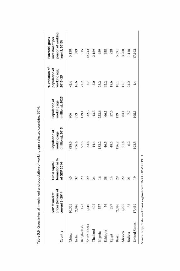
Tabl
e 5.
6 G
ross
inte
rnal
inve
stm
ent a
nd p
opul
atio
n of
wor
king
age
, sel
ecte
d co
untr
ies,
2014
.
Coun
try
GD
P at
mar
ket
pric
es (b
illio
ns o
f cu
rren
t $) 2
014
Gro
ss c
apita
l fo
rmat
ion
as %
of
GD
P 20
14
Popu
latio
n of
w
orki
ng a
ge
(mill
ions
), 20
15
Popu
latio
n of
w
orki
ng a
ge
(mill
ions
), 20
25
% v
aria
tion
of
popu
latio
n of
w
orki
ng a
ge,
2015
–25
Pote
ntia
l gro
ss
inve
stm
ent p
er
pers
on o
f wor
king
ag
e ($
, 201
5)
Chi
na10
,355
4692
8.6
906
−2.4
5,13
0In
dia
2,04
632
736.
685
916
.688
9Ba
ngla
desh
173
2997
.511
9.1
22.2
515
Sout
h K
orea
1,41
029
33.4
32.5
−2.7
12,2
43Th
aila
nd40
524
44.4
43.5
−2.0
2,18
9N
iger
ia55
716
182.
223
3.6
28.2
489
Ethi
opia
5638
46.5
66.1
42.2
458
Egyp
t28
714
48.5
57.5
18.6
828
Braz
il2,
346
2912
6.2
139
10.1
5,39
1M
exic
o1,
295
2271
.884
.117
.13,
968
Boliv
ia33
216.
27.
724
.21,
118
Uni
ted
Stat
es17
,419
1919
2.5
195.
11.
417
,193
Sour
ce: h
ttp://
data
.wor
ldba
nk.o
rg/in
dica
tor/
NY.
GD
P.M
KT
P.C
D
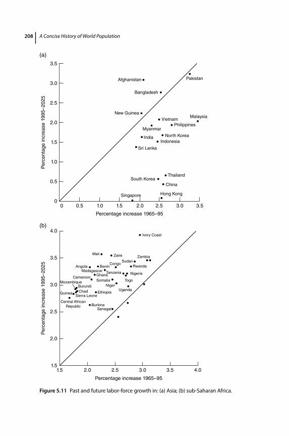
A Concise History of World Population208
00
0.5
0.5
1.0
1.0
Afghanistan Pakistan
Bangladesh
New GuineaVietnam
Malaysia
PhilippinesMyanmar
North KoreaIndonesia
India
Sri Lanka
ThailandSouth Korea
China
Hong KongSingapore
Percentage increase 1965–95
Percentage increase 1965–95
Per
cent
age
incr
ease
199
5–20
25P
erce
ntag
e in
crea
se 1
995–
2025
Ivory Coast
Mali Zaire ZambiaSudan
Rwanda
Togo
Nigeria
Uganda
CongoBenin
TanzaniaGhana
AngolaMadagascar
CameroonSomalia
Niger
Ethiopia
BurkinaSenegal
1.51.5
2.5
2.5
3.0
3.0
3.5
3.5
4.0
4.0
2.0
2.0
Sierra LeoneChadBurundi
Mozambique
Guinea
Central AfricanRepublic
1.5
1.5
2.0
2.0
2.5
2.5
3.0
3.0 3.5
3.5
(a)
(b)
Figure 5.11 Past and future labor‐force growth in: (a) Asia; (b) sub‐Saharan Africa.
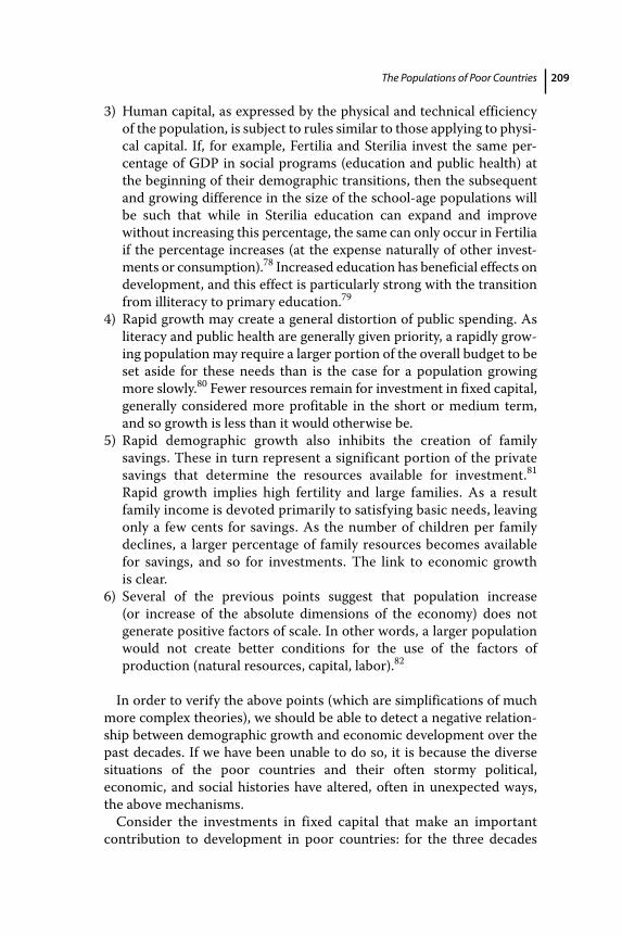
The Populations of Poor Countries 209
3) Human capital, as expressed by the physical and technical efficiency of the population, is subject to rules similar to those applying to physi-cal capital. If, for example, Fertilia and Sterilia invest the same per-centage of GDP in social programs (education and public health) at the beginning of their demographic transitions, then the subsequent and growing difference in the size of the school‐age populations will be such that while in Sterilia education can expand and improve w ithout increasing this percentage, the same can only occur in Fertilia if the percentage increases (at the expense naturally of other invest-ments or consumption).78 Increased education has beneficial effects on development, and this effect is particularly strong with the transition from illiteracy to primary education.79
4) Rapid growth may create a general distortion of public spending. As literacy and public health are generally given priority, a rapidly grow-ing population may require a larger portion of the overall budget to be set aside for these needs than is the case for a population growing more slowly.80 Fewer resources remain for investment in fixed capital, generally considered more profitable in the short or medium term, and so growth is less than it would otherwise be.
5) Rapid demographic growth also inhibits the creation of family s avings. These in turn represent a significant portion of the private savings that determine the resources available for investment.81 Rapid growth implies high fertility and large families. As a result family income is devoted primarily to satisfying basic needs, leaving only a few cents for savings. As the number of children per family declines, a larger percentage of family resources becomes available for savings, and so for investments. The link to economic growth is clear.
6) Several of the previous points suggest that population increase (or increase of the absolute dimensions of the economy) does not g enerate positive factors of scale. In other words, a larger population would not create better conditions for the use of the factors of p roduction (natural resources, capital, labor).82
In order to verify the above points (which are simplifications of much more complex theories), we should be able to detect a negative relation-ship between demographic growth and economic development over the past decades. If we have been unable to do so, it is because the diverse situations of the poor countries and their often stormy political, e conomic, and social histories have altered, often in unexpected ways, the above mechanisms.
Consider the investments in fixed capital that make an important contribution to development in poor countries: for the three decades
A Concise History of World Population210
following 1960 it has been estimated that about two‐thirds of output growth was the result of increased input of capital as compared to one‐quarter due to labor and one‐seventh to total factor productivity or tech-nical progress. In industrial countries, the contribution of fixed capital in the same period was much lower and estimated at between one‐quarter and one‐third of total growth.83 All things being equal, there should, in principle, exist a thinning effect on capital per worker in more rapidly growing populations.84 Many countries, particularly the poorest ones, have managed just the same to increase the percentage of their GDP devoted to investment: according to the World Bank, low‐income econo-mies increased this share from 20 to 30 percent between 1970 and 1993. In India and South Africa, between 1990 and 2009, the investment/GDP ratio has increased by 8–9 percentage points.85 In this way the “thinning effect” on capital exerted by rapid population growth has been at least partially neutralized.
With regard to fixed natural resources, especially land, the agricultural expansion that has enabled the developing countries as a whole to increase agricultural production at a greater rate than population is p rimarily due to increasing yields (the “green revolution”), rather than the cultivation of new lands.86 In fact, the introduction of green‐revolution technology in many areas has been aided by high population density, which favors infrastructure development and technology transfer.87 In other areas, however, the scarcity of land and its high cost have created serious obstacles.88
Recent studies have also cast doubt on the theory that rapid demo-graphic growth alters the proportions of public spending, favoring “social investments,” especially education, at the expense of investments in fixed capital. According to some, poor country rates of demographic growth have not affected the progress of literacy and education, nor have they distorted public spending to the detriment of investments in fixed capi-tal. More economical use of available resources (for example, limiting teachers’ salaries) has allowed for the realization of goals in spite of high demographic pressure.89 In the period since 1980, an increased propor-tion of resources in many countries has been c hanneled to education.90
With regard to the creation of savings, both theoretical and empiri-cal considerations challenge the assumption that rapidly growing population necessarily implies a lower rate of saving due to larger family size. Several possible mechanisms seem to neutralize this effect. The first is that adult labor intensity within the family does not remain fixed, but changes in response to changes in family size. A larger number of dependent c hildren leads to intensification of p roductive activity (particularly in rural areas), an increase in resources, and so perhaps also of savings.91 In his classic study of
The Populations of Poor Countries 211
peasant economies, Chayanov noted a clear r elationship between the number of dependants per worker and labor intensity in peasant fami-lies of Tsarist Russia. Intensity increased as families grew and declined as they shrank.92 In the second place, there is a higher ratio of young workers (who save) to old or retired workers (who have negative sav-ings) in a rapidly growing population, and this effect tends to balance out the negative impact on savings of a large number of dependent children.93 Finally, family savings in poor countries come primarily from a few very rich families and so are little influenced by family size. As things stand, the numerous tests of the relationship between demographic growth (not to mention age structure, dependency ratio, and so forth) and the rate of savings have not yielded significant results. Opposing forces seem to neutralize one another, and it may also be the case that insufficient data play an important role in the inconclusiveness of results.94
The final point concerns possible economies of scale, which I have already discussed (see Chapter 3, Section 5). Those who support the hypothesis of a negative correlation between demographic growth and economic development believe these to be nonexistent or at least i rrelevant. Others, however, hold that population growth and increasing density have fueled the development of infrastructure (especially com-munications and transportation) necessary for economic development.95 As mentioned above, in many countries agricultural development and the green revolution seem to be helped rather than hindered by higher demographic density, and so factors of scale, in a broad sense, seem to exercise a significant positive influence. One should also add the fact that the geographic situation of a country, its climatic and biopathological environment, its accessibility and natural conformation, and its endow-ment of primary resources, closely interact with the demographic and economic characteristics.96
The problems raised by consideration of the relationship between population and economy are intricate and involve variables whose inter-action and causal relationship with other factors are neither stable nor well understood. The above discussion may help to explain why the e volution of the relationship between population and economy in recent decades escapes simple theoretical schemes. The extreme adaptability of human behavior, both demographic and economic, in the face of external limitations confounds the simplifications of those who would like to translate this behavior into simple formulas for the sake of easy analysis. In addition, the helter‐skelter progress of technology blunts, expands, and distorts relationships often taken for granted.
Nonetheless, the fact that a clear and direct relationship between demographic growth and economic development is not readily discerned
A Concise History of World Population212
does not mean that it does not exist or that it is ultimately unmeasurable. The conclusions reached by A. C. Kelley in his in‐depth study of this problem are still relevant today:
Economic growth (as measured by per capita output) in many developing countries would have been more rapid in an environ-ment of slower population growth, although in a number of coun-tries the impact of population was probably negligible, and in some it may have been positive. Population’s adverse impact has most likely occurred where arable land and water are particularly scarce or costly to acquire, where property rights to land and n atural resources are poorly defined and where government policies are biased against the most abundant factor of production – labor. Population’s positive impact most likely occurred where natural resources are abundant, where the possibilities for scale economies are substantial, and where markets and other institutions (especially government) allocate resources in a reasonably efficient way over time and space.97
Therefore, between the demographic paths taken by Fertilia and Sterilia, the choice will generally be for that of Sterilia, though we should keep in mind that this choice may not always be a successful one.
Notes
1 In this chapter I shall use the term “poor countries” for those countries frequently described as “less‐developed” or “developing,” and “rich countries” for those usually called “developed” or “more‐developed.” Rich and poor countries are of course abstract categories and serve primarily as a scheme of definition. The rich countries include the countries of Europe and North America, Australia, New Zealand, and Japan; by a considerable stretch of imagination, the countries of eastern Europe are also included. Occasionally I shall use the term “western countries” to refer to the c ountries of western Europe and their projections in North America and Oceania, excluding Japan, which has a distinct demographic history. Among the “poor” or developing countries the reader will find countries, such as South Korea, with current high standards of living, but that have emerged from poverty only in the past two or three decades. For a comparative analysis of the demographic transition in the poor and rich c ountries, see D. S. Reher, “The Demographic Transition Revisited as a Global Process,” Population, Space and Place 10 (2004). A good synthesis can be found in World Bank Group, Global Monitoring Report
The Populations of Poor Countries 213
2015/16: Development Goals in an Era of Demographic Change (Washington, DC, World Bank 2016).
2 The 28 countries considered are not in absolute terms the 25 most populous countries of the poor world, but rather the most populous from each continent: nine in Africa (Democratic Republic of the Congo, Egypt, Ethiopia, Kenya, Morocco, Nigeria, South Africa, Sudan, and Tanzania), 11 in Asia (Bangladesh, China, India, Indonesia, Iran, Pakistan, the Philippines, South Korea, Thailand, Turkey, and Vietnam), and 8 in America (Argentina, Brazil, Chile, Colombia, Cuba, Mexico, Peru, and Venezuela). The combined population of these countries represents well over four‐fifths of the total population of the poor countries. From the point of view of their history and demographic growth, Argentina and Chile have more in common with the European countries (of which they are “projections”) than with other Latin American countries. The exclusion of small countries – such as Hong Kong, Singapore, Mauritius, Costa Rica, and Taiwan – eliminates interesting cases of precocious transition, processes which, however, are in part favored by their small dimensions or insularity.
3 On the phases of the mortality transition in the various continents, see J. C. Riley, “The Timing and Pace of Health Transition Around the World,” Population and Development Review 31:4 (2005).
4 United Nations, World Population Prospects. The 2015 Revision (New York, 2015). M. Mahy, Childhood Mortality in the Developing World: A Review of Evidence from the Demographic and Health Surveys, DHS Comparative Reports, no. 4 (ORC Macro, Calverton, MD, 2003).
5 These figures are calculated assuming that mortality beyond age 5 for these “new survivors” is that of the respective areas.
6 ORT, or oral rehydration therapy. These are simple packets, the contents of which are soluble in water and contain the essential salts lost by the infant suffering attacks of diarrhea; the afflicted baby, by drinking this solution, is able to make up for these losses. It is a therapy easily administered by the child’s mother or another family member. When this is too expensive, a simple sugar–salt–water solution can provide enough of the fluids, calories, and salt an infant needs to recover from diarrhea. On childhood pathologies and their care, see R. Y. Stallings, Child Morbidity and Treatment Patterns, DHS Comparative Reports, no. 8 (ORC Macro, Calverton, MD, 2004).
7 The countries represented in Figures 5.4 and 5.7 are listed in note 2.8 These include not only the smallpox vaccine – smallpox virtually
disappeared at the end of the 1970s – but also vaccines against measles, whooping cough, neonatal tetanus contracted at birth as a result of umbilical cord infection, polio, tuberculosis, and diphtheria, which claim millions of victims. See “Immunizing the World’s Children,” Population Reports, series L (Mar.–Apr. 1986).
A Concise History of World Population214
9 S. A. Meegama, “The Mortality Transition in Sri Lanka,” in Determinants of Mortality Change and Differentials in Developing Countries (United Nations, New York, 1986).
10 W. H. Mosley, “Will Primary Health Care Reduce Infant and Child Mortality? A Critique of Some Current Strategies with Special Reference to Africa and Asia,” in J. Vallin and A. D. Lopez, eds., Health Policy, Social Policy and Mortality Prospects (INED/IUSSP, Ordina, Liège, 1985).
11 WHO–UNICEF, Alma Ata 1978: Primary Health Care (WHO, Geneva, 1978); WHO, World Health Report 2003: Shaping the Future (WHO, Geneva, 2003, Chapter 7).
12 A. Sen, “Health in Development,” Bulletin of the World Health Organization 77 (1999), p. 8; A. Sen, “The Economics of Life and Death,” Scientific American (May 1993), pp. 18–25.
13 This is the point of view expressed in J. C. Caldwell, “Routes to Low Mortality in Poor Countries,” Population and Development Review 12:4 (1986).
14 Caldwell, “Routes to Low Mortality in Poor Countries,” pp. 209–11. On mortality trends in developing countries, see also R. R. Soares, “On the Determinants of Mortality Reductions in the Developing World,” Population and Development Review 33:2 (2007); R. Kuhn, “Routes to Low Mortality in Poor Countries Revisited,” Population and Development Review 36:4 (2010).
15 In fact, in some countries of sub‐Saharan Africa there has been clear evidence of an increase in fertility – an increase explained by shorter breast‐feeding, and so reduced birth intervals (see later in this section), and by improved sanitary conditions, which have reduced the incidence of certain infectious diseases causing sterility or reduced fecundity. The UN, for example, estimates that the TFR for western Africa increased from 6.7 to 6.9 between 1950–5 and 1975–80 and that of eastern Africa from 6.7 to 7. M. Garenne, Fertility Changes in Sub‐Saharan Africa, DHS Comparative Reports no. 18 (ORC Macro, Calverton, MD, 2008). For a general appraisal of fertility trends, see United Nations, World Fertility Report 2013. Fertility at the Extremes (UN, New York, 2014).
16 Naturally, this analogy is only applicable in a general sense, and the attendant circumstances were very different. Mortality decline in Europe came about more gradually and so allowed a gradual adjustment of fertility. Moreover, even in high‐fertility areas birth control was practiced by a significant sector of society, such as the urban classes and the well‐educated. On the other hand, current developments in many less‐developed countries show that fertility may fall below replacement replicating the recent history of the rich countries. See D. S. Reher, “Long‐Term Population Decline, Past and Future,” XXV International Population Conference, Tours, 2005. According to the UN evaluations, the number of low fertility countries (TFR of 2 or less) has increased from 51 in 1994 to 70 in 2014. See: United Nations, World Fertility Report 2013.
The Populations of Poor Countries 215
17 DHS surveys have been taken since 1986 in a large number of countries of the developing world on samples of women of reproductive age ranging in size from 2,000 to 30,000 persons. The survey questionnaire includes questions on demographic characteristics, fertility history, contraceptive use, and health of women and children, as well as many socioeconomic variables. Several countries have had more than one survey, and in many cases samples of men and husbands have also been included. See DHS + Dimension, Newsletter 3:1 (2001), 3:7 (2005).
18 G. Mboup and T. Saha, “Fertility Levels, Trends and Differentials,” Comparative Studies 28 (Macro International, Calverton, MD, 1999). On the slow fertility transition in Africa south of the Sahara, see A. Romaniuk, “Persistence of High Fertility in Tropical Africa,” Population and Development Review 7:1 (2011).
19 On the general characteristics and principal results of the World Fertility Survey, see WFS, Major Findings and Implications (London, 1984). The surveys, normally carried out on groups of 3,000–10,000 women of reproductive age, comprised 41 developing countries and 21 developed countries; most were conducted in the second half of the 1970s.
20 United Nations, Fertility Behavior in the Context of Development. Evidence from the World Fertility Survey (UN, New York, 1987), pp. 78, 82; United Nations, First Marriage: Patterns and Determinants (UN, New York, 1988).
21 The World Bank, World Development Report 1984 (Oxford University Press, New York, 1984), pp. 115–16. United Nations, Fertility Behavior, p. 78. See also P. Xenos and S. A. Gultiano, Trends in Female and Male Marriage and Celibacy in Asia, in “Papers of the Program in Population,” no. 120 (East–West Center, Honolulu, 1992); C. Westoff, A. K. Blanc, and L. Nyblade, Marriage and Entry into Parenthood, DHS Comparative Studies no. 10 (1994).
22 Mboup and Saha, Fertility Levels; J. Bongaarts, “The Fertility Impact of Changes in the Timing of Childbearing in the Developing World,” Working Paper, no. 120 (Population Council, New York, 1999); “World Marriage Patterns 2000,” Population Newsletter (December, 1999); United Nations, World Population Monitoring. Reproductive Rights and Reproductive Health (UN, New York, 2003), pp. 133–5. United Nations, World Fertility Report 2013, pp. 37–41
23 W. P. Mauldin and S. J. Segal, “Prevalence of Contraceptive Use: Trends and Issues,” Studies in Family Planning 19 (1988), p. 340. Of course these measures only give a very general picture, as the effectiveness of the various contraceptive methods depends in part on the method itself (the pill and IUD are highly effective while coitus interruptus and rhythm are not) and in part on the motivation and assiduousness of the couple. M. Garenne, “Trends in marriage and contraception in sub‐Saharan Africa: A longitudinal perspective on factors of fertility
A Concise History of World Population216
decline,” (DHS Analytical Studies No. 42. ICF International Rockville, Maryland, 2014).
24 United Nations, Fertility Behavior, p. 133.25 Data are available online, http://www.dhsprogram.com/26 The World Bank, World Development Report 1984 (New York, Oxford
University Press, 1984), pp. 115–16.27 The fertility‐reducing impact of the increase of age at marriage is relatively
modest and gradual, as is shown by the experience since the 1940s.28 R. D. Lee and R. A. Bulatao, “The Demand for Children: A Critical
Essay,” in R. D. Lee and R. A. Bulatao, eds., Determinants of Fertility in Developing Countries, vol. 1 (Academic Press, New York, 1983).
29 For differing interpretations regarding the cost of children, see J. C. Caldwell, “Direct Economic Costs and Benefits of Children” and P. H. Lindert, “The Changing Economic Costs and Benefits of Having Children,” both in Lee and Bulatao, Determinants of Fertility.
30 The World Bank, World Development Report 1984, p. 52.31 M. Cain, “Risk and Insurance: Perspectives on Fertility and Agrarian
Change in India and Bangladesh,” Population and Development Review 7:3 (1981). As to parents’ expectations concerning their own children’s support in old age: A. I. Hermalin and Li‐Shou Yang, “Levels of Support from Children in Taiwan: Expectations Versus Reality,” Population and Development Review 30:3 (2004).
32 This really only applies to developing countries. In the West almost the entire fertility transition took place by means of traditional methods like coitus interruptus. In fact, in most of the West the distribution and advertisement of birth‐control methods was illegal until after World War II.
33 United Nations, Report of the United Nations World Population Conference (UN, New York, 1975).
34 United Nations, Report of the International Conference on Population, 1984 (UN, New York, 1984).
35 United Nations, International Conference on Population and Development, Programme of Action, Cairo, 1994. On the international action after 1994: United Nations, Review and Appraisal of the Progress Made in Achieving the Goals and Objectives of the Programme of Action on the International Conference on Population and Development (UN, New York, 2004); UNFPA, ICPD at 15 – Report. Looking Back, Moving Forward (UN, New York, 2011).
36 J. Bongaarts, The Role of Family Planning Programs in Contemporary Fertility Transition, Working Paper, no. 71 (Population Council, New York, 1995).
37 On unmet need, see J. Bongaarts and J. Bruce, The Causes of Unmet Need for Contraception and the Social Content of Services, Working
The Populations of Poor Countries 217
Paper, no. 69 (Population Council, New York, 1994); C. F. Westoff and A. Bankole, Unmet Need: 1990–94, DHS Comparative Studies no. 16 (Macro International, Calverton, MD, 1995). United Nations, World Fertility Report 2013, pp. 42–43.
38 P. W. Mauldin and J. A. Ross, “Family Planning Programs: Efforts and Results,” Studies in Family Planning 22:6 (1991).
39 J. Bongaarts, The Fertility Impact of Family Planning Programs (Population Council, New York, 1993), p. 4.
40 Of the 46 countries, 22 are from sub‐Saharan Africa, 10 from Asia and North Africa, 10 from Latin America, four from Europe.
41 For an effective criticism of the conventional view and a demand‐ oriented approach, see L. H. Pritchett, “Desired Fertility and the Impact of Population Policies,” Population and Development Review 20:1 (1994).
42 Prevalence of contraception is defined as the percentage of currently married women, age 15–49, currently using any method. Wanted fertility (WTFR) is close, but not identical, to the concept of “desired fertility.” This can be assessed on the basis of answers to the DHS survey question: “If you could go back to the time you did not have any children and could choose exactly the number of children to have in your whole life, how many would that be?” Subtracting from the number of actual births those births in excess of each woman’s desires, a desired total fertility rate (DTFR) is computed. Answers to the question on desired fertility are obviously influenced by the mothers’ rationalization of past behavior. Alternatively, wanted fertility can be estimated indirectly using answers to the question about desires for future births. This answer refers to the future and not to the past, and is not biased by ex‐post rationalization. Past births to women who want another child are classified as wanted and, with other adjustments, a measure of total wanted fertility is e stimated (WTFR). For desired fertility, see C. Westoff, “Reproductive Preferences: A Comparative View,” Demographic and Health Surveys, Comparative Studies, no. 3 (IRD/Macro Systems, Columbia, MD, 1991). For the concept of wanted fertility, see J. Bongaarts, “The Measurement of Wanted Fertility,” Population and Development Review 16:3 (1990). For a discussion of the various measures, see Pritchett, “Desired Fertility.”
43 Defined as (TFR − WTFR)/TFR × 100.44 Pritchett, “Desired Fertility,” p. 15. For a contrary view, see B. Feyisetan
and J. B. Casterline, Fertility Preferences and Contraceptive Change in Developing Countries, Working Paper, no. 130 (Population Council, New York, 1999).
45 P. Demeny, “Policies Seeking a Reduction of High Fertility,” in United Nations, Population Policies and Programmes (UN, New York, 1993).
46 “Law and Policy Affecting Fertility: A Decade of Change,” Population Reports, series E (Nov. 1984), p. E–117.
A Concise History of World Population218
47 A. Mitra, “National Population Policy in Relation to National Planning in India,” Population and Development Review 3:3 (1977); A. J. Coale, “Population Trends in India and China,” Proceedings of the National Academy of Sciences 80 (1983), p. 1,759.
48 Mauldin and Segal, “Prevalence of Contraceptive Use,” Table A.3.49 K. Singh, “National Population Policy: A Statement of the Government
of India,” Population and Development Review 2:2 (1976).50 Mitra, “National Population Policy in India,” p. 207.51 United Nations, Population Policy Briefs: The Current Situation in
Developing Countries, 1985 (New York, 1986).52 Coale, “Population Trends,” p. 1,760.53 United Nations, Review of Recent Demographic Target‐Setting (New
York, 1989), pp. 96–108.54 D. Banrji, “Population Policies and Programmes in India during the Last Ten
Years,” in S. N. Singh, M. K. Premi, P. S. Bhatia, and A. Bose, eds., Population Transition in India, vol. 1 (B. R. Publishing, New Delhi, 1989), p. 49.
55 Speech of Rajiv Gandhi inaugurating the 21st General Conference of the International Union for the Scientific Study of Population (IUSSP), New Delhi, September 20, 1989: “Yet, to a large extent, our family planning programs are more or less uniform throughout the country. Virtually the same package is delivered to the high population growth areas as to the low population growth areas … each couple’s perception, especially the woman’s perception, of the desired family size … is most influenced by the desires and ethos of the local community or neighborhood. How could this be determined monolithically by a central agency?”
56 Populi 22:4 (1995) p. 2; East–West Center, “New Survey Finds Fertility Decline in India,” Asian Pacific Population Policy 32 (Jan.–Feb. 1995); International Institute for Population Studies and ORC Macro, National Family Health Survey (NFHS‐2), India, 1998–99 (IIPS, Mumbai, 2000), National Family Health Survey (NFHS‐2), India, 2005–06; “India Considers Adopting Family Planning Incentives,” Popline 22 (Mar.–Apr. 2000). Ministry of Health and Family Welfare, National Health Policy 2015, New Delhi, 2014, http://www.mohfw.nic.in/WriteReadData/l892s/35367973441419937754.pdf, accessed July 22, 2016.
57 On Chinese population policy until the 1980s, M. Aglietti, La politica di pianificazione familiar in Cina dalla Fondazione della Repubblica a oggi [The Family Planning Policy in China from the Founding of the Republic to the Present Day], degree thesis in Demography, Political Science Faculty, University of Florence, 1987. See also T. Scharping, Birth Control in China, 1949–2000 (RoutledgeCurzon, London and New York, 2003); “Population and Birth Planning in the People’s Republic of China,” Population Reports, series J (January–February 1982); J. Banister, China’s Changing Population (Stanford University Press, Stanford, CA, 1987).
58 Aglietti, La politica, p. 20.

The Populations of Poor Countries 219
59 Aglietti, La politica, p. 28.60 Aglietti, La politica, pp. 152–3.61 “Population and Birth Planning in China,” p. 590.62 Aglietti, La politica, p. 217.63 K. Hardee‐Cleaveland and J. Banister, “Fertility Policy and
Implementation in China,” Population and Development Review 14:2 (1988), p. 247.
64 “China’s Experience in Population Matters: An Official Statement,” Population and Development Review 20:2 (1994); text read before the 27th Session of the United Nations Population Commission on March 28, 1994, by Peng Yu, China’s representative to the Commission. The text also refers to the official population policy guidelines.
65 Jiali Li, Population Council Working Paper no. 65 (1994). Out of a sample of permissions granted to rural couples for second or higher‐order births in the province of Hebei in 1983–8, 33 percent were granted because the first child had died or was disabled; 7 percent owing to remarriage; 25 percent because the couple lived in a remote area or had special characteristics (belonged to a minority or one member worked as a miner, was disabled, etc.); 14 percent because a “special permit” was granted; 21 percent because of the desire to have a male child who could carry on the family line.
66 S. Greenhalgh, C. Zhu, and N. Li, “Restraining Population Growth in Three Chinese Villages,” Population and Development Review 20:2 (1994).
67 Greenhalgh et al., “Restraining Population Growth,” pp. 382–9.68 For a survey of recent demographic and policy trends in China, see
Wang Feng, “Can China Afford to Continue Its One‐Child Policy?,” Asia Pacific Issues 77 (March, 2005); T. Scharping, Birth Control in China; Zeng Yi, “Options for Fertility Policy Transition in China,” Population and Development Review 33:2 (2007); Gu Baochang, Wang Feng, Guo Zhizang, and Zhang Erli, “China’s Local and National Fertility Policies at the End of the Twentieth Century,” Population and Development Review 33:1 (2007); S. P. Morgan, Z. Guo, and S. R. Hayford, “China’s Below Replacement Fertility: Recent Trends and Future Prospects,” Population and Development Review 25:3 (2009);Y. Cai, “China’s Below Replacement Fertility: Government Policy or Socio‐Economic Development?,” Population and Development Review 36:3 (2010); Y. Cai, F. Wang, Z. Zheng, and B. Gu, “Fertility Intention and Fertility Behavior: Why Stop at One?,” paper presented at the Population Association of America meeting, Dallas, TX, April 15–17, 2010; Z. Zhao, “Closing a Sociodemographic Chapter of Chinese History,” Population and Development Review, 41:5 (2015).
69 Communiqué of the Fifth Plenary Session of the Eighteenth Central Committee of the Communist Party of China, Xinhua News Agency, Beijing, October 29, 2015. Zhao, “Closing a Sociodemographic Chapter.”
A Concise History of World Population220
70 Coale, “Population Trends,” p. 1,761.71 I am indebted to a well‐known scholar both for the idea and the names
of Fertilia and Sterilia. See J. E. Meade, “Population Explosion, the Standard of Living and Social Conflict,” Economic Journal 77 (1967). The example of the two islands of Fertilia and Sterilia is found on pp. 239–42, together with many incisive observations about the relationship between demographic growth and economic development. My attempt to find alternative names to Fertilia and Sterilia and so avoid the above plagiarism met with no success.
72 For the list of countries see note 2.73 In an overview of the relationship between population and develop-
ment, Robert Cassen writes: “Altogether simple economics seems to suggest that countries with faster population growth will in the long run end up with lower per capita income … But neither theory nor econo-metrics has so far been able to demonstrate this relationship beyond doubt.” See R. Cassen, “Overview,” in R. Cassen, ed., Population and Development: Old Debates, New Conclusions (Transaction Publishers, New Brunswick, NJ, 1994), pp. 10–11. For Ansley Coale, the lack of association between population and economic growth is due to the banal fact that population growth is (migration aside) the difference between birth and death rates, and both of these have strong inverse relations with the gradient of development. As a consequence, the same rate of population growth can occur at different levels of development, blurring any visible relation with the speed of economic growth. See A. Coale, “Population Trends and Economic Development,” in J. Menken, ed., World Population and the U.S. Policy: The Choices Ahead (W. W. Norton, New York, 1986).
74 There is considerable literature on this topic. I shall cite several works that seem to me fundamental both for their broad scope and systematic approach: The World Bank, World Development Report 1984, esp. chapters 5 and 6; G. McNicoll, “Consequences of Rapid Population Growth: An Overview and Assessment,” Population and Development Review 10:2 (1984); E. Hammel et al., Population Growth and Economic Development: Policy Questions (National Academy Press, Washington, DC, 1986); A. C. Kelley, “Economic Consequences of Population Change in the Third World,” Journal of Economic Literature 26, 1,685–728 (1988); Cassen, Population and Development. A. C. Kelley and R. M. Schmidt, “Economic and Demographic Change: A Synthesis of Models, Findings and Perspectives,” in N. Birdsall, A. C. Kelley, and S. W. Sinding, eds., Population Matters (Oxford University Press, New York, 2001); D. D. Headey and A. Hodge, “The Effect of Population Growth on Economic Growth,” Population and Development Review 35:2 (2009). According to the review of the literature made by these
The Populations of Poor Countries 221
latter authors, the negative relation between population growth and economic development is more evident after 1980.
75 On this and the following points, see the classic work of A. J. Coale and E. M. Hoover, Population Growth and Economic Development in Low‐Income Countries (Princeton University Press, Princeton, NJ, 1958), pp. 19–20.
76 R. Eastwood and M. Lipton, “Demographic Transition in Sub‐Saharan Africa: How Big Will the Demographic Dividend Be?” Population Studies 65:1 (2011).
77 J. Bauer, “Demographic Change and Asian Labor Markets in the 1990s,” Population and Development Review 16:4 (1990) p. 631.
78 Coale and Hoover, Population Growth, p. 25.79 A study of a group of developing countries has shown that increasing the
average amount of education of the labor force by 1 year raises GDP by 9 percent; this rate of improvement, however, only holds for the first 3 years of education, after which the return for an additional year of education diminishes to about 4 percent. See The World Bank, World Development Report 1991 (Oxford University Press, New York, 1991), p. 43.
80 Coale and Hoover, Population Growth, p. 285.81 Coale and Hoover, Population Growth, p. 25.82 With regard to the minimal relevance of factors of scale in the manufactur-
ing industries, see National Research Council, Population Growth, p. 52.83 The World Bank, World Development Report 1991 (Oxford University
Press, New York, 1991), p. 45. See also E. F. Denison, Trends in American Economic Growth (Brookings Institution, Washington, DC, 1985), who estimates that the contribution of capital accumulation to US GDP growth between 1929 and 1982 was less than one‐fifth. See also A. Maddison, Phases of Capitalism Development (Oxford University Press, Oxford, 1982), pp. 23–4; Kelley, “Economic Consequences of Population Change,” pp. 1,704–5.
84 National Research Council, Population Growth, pp. 40–6.85 The World Bank, World Development Report 1995 (Oxford University
Press, New York, 1995), Table 9. For India, South Africa, and other countries see http://data.un.org/Explorer.aspx
86 Y. Hayami and V. W. Ruttan, “The Green Revolution: Inducement and Distribution,” Pakistan Development Review 23, 38–63 (1984); see also The World Bank, World Development Report 1993, p. 135 for regional estimates of the contribution of variation of areas and yields to cereal production.
87 P. L. Pingali and H. R. Binswangen, “Population Density and Agriculture Intensification: A Study of the Evolution of Technologies in Tropical Agriculture,” in D. G. Johnson and R. D. Lee, eds., Population Growth and Economic Development (University of Wisconsin Press, Madison, 1987).
88 Kelley, “Economic Consequences of Population Change,” pp. 1,712–15.
A Concise History of World Population222
89 T. P. Schultz, “School Expenditures and Enrollments, 1960–1980: The Effects of Income, Prices and Population Growth,” in Johnson and Lee, Population Growth; see also J. G. Williamson, “Human Capital Deepening, Inequality and Demographic Events along the Asia‐Pacific Rim,” in N. Ogawa, G.W. Jones, and J. G. Williamson, eds., Human Resources in Development along the Asia‐Pacific Rim (Oxford University Press, Singapore, 1993); Crook, Principles of Population, pp. 203–5.
90 A. Cammelli, “La Qualità del Capitale Umano [The Quality of Human Captial],” in M. Livi‐Bacci and F. Veronesi Martuzzi, eds., Le Risorse Umane del Mediterraneo [Mediterraneon Human Resources] (Il Mulino, Bologna, 1990).
91 For a review of the relationship between demographic growth and savings, see A. Mason, “Saving, Economic Growth, and Demographic Change,” Population and Development Review 14:1 (1988); Kelley, “Economic Consequences of Population Change,” pp. 1,706–8; The World Bank, World Development, pp. 82–4.
92 A. V. Chayanov, The Theory of Peasant Economy (Irwin, Homewood, IL, 1966). For a more systematic and up‐to‐date treatment see J. Simon, The Economics of Population Growth (Princeton University Press, Princeton, NJ, 1977), pp. 185–95.
93 National Research Council, Population Growth, p. 43.94 National Research Council, Population Growth, pp. 43–5; Kelley,
“Economic Consequences of Population Change,” pp. 1,706–7.95 Simon, Economics of Population Growth, pp. 262–77.96 These are considerations that are as obvious as they are frequently
forgotten. See J. Sachs, Tropical Underdevelopment, NBER, Working Paper, no. 8119 (Cambridge, MA, 2001); J. Sachs, The End of Poverty: How We Can Make it Happen in Our Lifetime (Penguin, London, 2005).
97 Kelley, “Economic Consequences of Population Change,” p. 1,715. See also A. C. Kelley and W. P. McGreevey, “Population and Development in Historical Perspective,” in Cassen, Population and Development. For a view of the demographic goals to be achieved in order to sustain development, see United Nations, Population Challenges and Development Goals (UN, New York, 2005).
Further Reading
J. Banister, China’s Changing Population (Stanford University Press, Stanford, CA, 1987).
R. A. Bulatao and R. D. Lee, eds., Determinants of Fertility in Developing Countries, 2 vols. (Academic Press, New York, 1983).
The Populations of Poor Countries 223
J. Casterline, “The Onset and Pace of Fertility Transition: National Patterns in the Second Half of the Twentieth Century,” Population and Development Review (supplement to vol. 27, 2001).
A. J. Coale and E. M. Hoover, Population Growth and Economic Development in Low‐Income Countries (Princeton University Press, Princeton, NJ, 1958).
K. Davis, The Population of India and Pakistan (Russell & Russell, New York, 1968 [1951]).
A. Deaton, The Great Escape: Health, Wealth and the Origins of Inequality (Princeton University Press, Princeton, 2013).
R. D. Lee and D. S. Reher, eds., “Demographic Transition and Its Consequences,” Population and Development Review (supplement to vol. 37, 2011).
M. R. Montgomery and B. Cohen, eds., From Death to Birth: Mortality Decline and Reproductive Change (National Academy Press, Washington, DC, 1998).
A. Sen, Poverty and Famines (Clarendon Press, Oxford, 1981).Xizhe Peng, ed., The Changing Population of China (Blackwell, Oxford, 2000).WHO, World Health Report 2010 (Geneva, 2011).
225
A Concise History of World Population, Sixth Edition. Massimo Livi-Bacci. © 2017 John Wiley & Sons Ltd. Published 2017 by John Wiley & Sons Ltd.
The Future
6.1 Population and Self‐Regulation
Two centuries ago, in the process of achieving greater demographic order and efficiency, the human population embarked upon an unprecedented cycle of growth; while this cycle has come to an end in the rich countries, it is still in full swing in the poor ones. World population hit the 1 billion mark as steam engines began to revolutionize transportation; the second billion was reached after World War I, as airplanes became an ever more common means of transportation; the third billion was achieved at the beginning of the aerospace era. The fourth and fifth billion marks did not wait for similar revolutionary epochs and were reached in 1974 and 1987; the sixth was achieved in 1998, the seventh in 2012. Many demographers, sure of winning, would be willing to bet that the eighth billion will come in 2023. The combination of current young age structures and high f ertility ensures that this level will be easily reached within this time frame. Longer‐term prediction rapidly loses certainty, becoming eventually a purely mathematical exercise. This uncertainty, however, will not deter us from considering potential population growth well into the twenty‐first century.
Many view this growth process like a spring that is ever more tightly compressed, ready at the first jolt to unload an accumulation of devastating force. From an economic point of view diminishing returns must sooner or later lower living standards, since land, water, air, and minerals are all fixed and limited resources, allowing only partial substitution and therefore bound to place a limit on growth. The link between d emographic growth and environmental deterioration also seems clear, judging from the pollution caused by industrial expansion and the general ecological degradation associated with the increase of agricultural, industrial, r esidential, and other human activity. And demographic growth is also a threat to health and social order, given the impossibility of indefinitely
6
A Concise History of World Population226
expanding food production and the inevitability of competition and c onflict between individuals, groups, and peoples in search of a higher standard of living.
Another camp, instead, has complete faith in the ability of populations to adjust to larger numbers. Technological progress, they point out, allows for the substitution of primary resources and leads to increasing agricultural production. In addition, the relative prices of energy, p rimary resources, and food are at historically low levels and, in any case, the market would react to scarcity by increasing prices and so stimulating technological progress, guaranteeing increased productivity and the p ossibility of resource substitution. With regard to the costs of unregulated production, currently paid for by humanity at large in the form of environmental deterioration, population optimists maintain that these costs can be “internalized” – that is, paid for by those responsible. Their final argument is that the physical and economic well‐being of world population is constantly improving as a result of scientific and economic progress, and there is no reason to fear that this situation might change.
It is difficult, if not impossible, to choose between these two modes of foreseeing the future. Once again we return to the Malthusian model and, with regard to the more radical versions of the above arguments, what seems to be a revival of the catastrophist versus optimist debate. However, perhaps the debate itself misses the point and the problem can be better understood by employing an alternative approach, referred to in earlier chapters. I have presented the history of population as a c ontinual compromise between the forces of constraint and the forces of choice. Constraints have been imposed by a hostile environment, by d isease, by the limitations of available food and energy, and now by an environment in danger. Choices have included flexible strategies of m arriage and reproduction, of mobility, migration, and settlement, and of defense from disease. This interaction between the forces of constraint and choice has continually altered the point of population equilibrium and generated long cycles of growth as well as phases of stagnation and regression. The continuous dynamic search for equilibrium should not be seen as the product of spontaneous self‐regulating mechanisms that minimize suffering and loss, but rather as a difficult process of adaptation that rewards more flexible populations while penalizing those more fragile and rigid ones. Many populations have succeeded at self‐regulation, while others either have not or have done so too late, paying a heavy price in the form of increased mortality, demographic regression, or in some cases, extinction. In the case of yet other populations, mistaken decisions have impaired defensive ability in the face of catastrophe, increasing demographic vulnerability.1
The Future 227
Looking to the future, we should reflect not only on the certain numerical growth of the coming decades (and the conjectural growth of the longer run), but also on the mechanisms of “choice” available to humanity and whether or not they are adequate in the face of external constraints and more or less efficient than in the past.
6.2 The Numbers of the Future
I have already mentioned that present‐day populations are characterized by considerable momentum and so demographic projections for the next couple of decades are fairly plausible. For example, in 2035 the population aged over 20 will come from generations born before 2015, which is to say from generations already born and counted; one need only subtract mortality, which is fairly stable over time. On the other hand, the size of the population aged under 20, which will be born between 2015 and 2035, is an unknown and depends upon two variables. The first of these variables, the size of the population of reproductive age, is not a mystery, as again, almost all of those who will enter their fecund period in the next 20 years have already been born. The second, unknown, variable is the propensity of this population to bear children, and on this point we can at best make a good guess. In the longer term, projections become increasingly uncertain, even when they are based on sophisticated esthetically appealing methodologies, and assume the role of illustrative “scenarios” rather than that of realistic probes into the future. Undeterred by these considerations I will illustrate the results of projections until the end of the century, that is, three generations into the future: these projections are based on hypotheses concerning the reproductive behavior of women (and men) who are not yet born, as well as of their children and of the children of their children … who will make their own decisions in the societal contexts of 30, 60, or 90 years into the future.
Within shorter horizons – a few decades from now – population p rojections are made easier by the considerable force of inertia of demographic change. Population inertia (or momentum) can be measured in several ways.2 One of these consists of imagining that populations, say from today, adopt (and do not subsequently abandon) replacement fertility – which, as we know, will eventually lead to a stationary population (zero growth) – while mortality remains fixed and net migration equals zero. Nonetheless, if the population in question has had, until recently, a high level of fertility and therefore possesses a young age structure (as in many developing countries) it will continue to grow for a certain period of time. In the following decades the many recently born children will
A Concise History of World Population228
enter reproductive age and, even if each of them bears few children, being numerous they will nonetheless produce a large total number of births. These births in turn will far outnumber deaths, as the latter will come primarily from the elderly, who belong to the smaller generations born many decades ago when population was far less than today. As those born under the new fertility regime begin to reach reproductive age, the number of births will gradually decline until it is approximately equal to the number of deaths. For instance, according to United Nations projections (medium variant, 2015 revision), the population of the poor countries is expected to grow from 6.1 to 8.4 billion between 2015 and 2050; however, even with replacement fertility, from 2015 onward, this population would still grow to 7.9 billion in 2050. This growth of 1.8 b illion – instead of the expected 2.3 – is the consequence of current young age structure, or of the present inertia, or momentum.
The United Nations has for some time made accurate projections, periodically revised, of the evolution of world population.3 Table 6.1 includes some of the principal results of retrospective estimates and so‐called medium variant projections through 2050. The latter are based on the fertility and mortality evolution considered most plausible, namely that the fertility of the less‐developed countries will continue to decline, from 2.65 children per woman in 2010–15 to 2.15 in 2045–50, and life expectancy at birth will increase in the same period from 69 to 75 years; for the developed countries it is predicted that there will be a mild f ertility recovery (from 1.7 to 1.9) and a further increase in life expectancy (from 78 to 83).
The most interesting results of this projection are the following:
1) World population will reach 8 billion in 2023 and 9 billion in 2037.42) The world rate of population increase, equal to 1.1 percent in 2010–15,
will gradually decline to 0.4 percent in 2045–50.3) However, as this decreasing rate of increase nonetheless applies to an
ever‐larger population, absolute annual increase of 84 million in 2010–15 will gradually decline to 54 million in 2045–50.
4) The target population of 9.7 billion for the year 2050 depends on the projected decline of fertility, which – for the world as a whole – should drop from an estimated TFR of 2.51 in 2010–15 to a projected 2.25 in 2045–50. Any decimal fraction of TFR above or below the 2.25 target at the end of the period will imply roughly 220 million inhabitants more, or less, in 2050.
5) The developing countries will account for almost all of the world population increase in the period 2010–50.
6) Geodemographic changes will be considerable: between 2015 and 2050 the developed country share of world population will decline
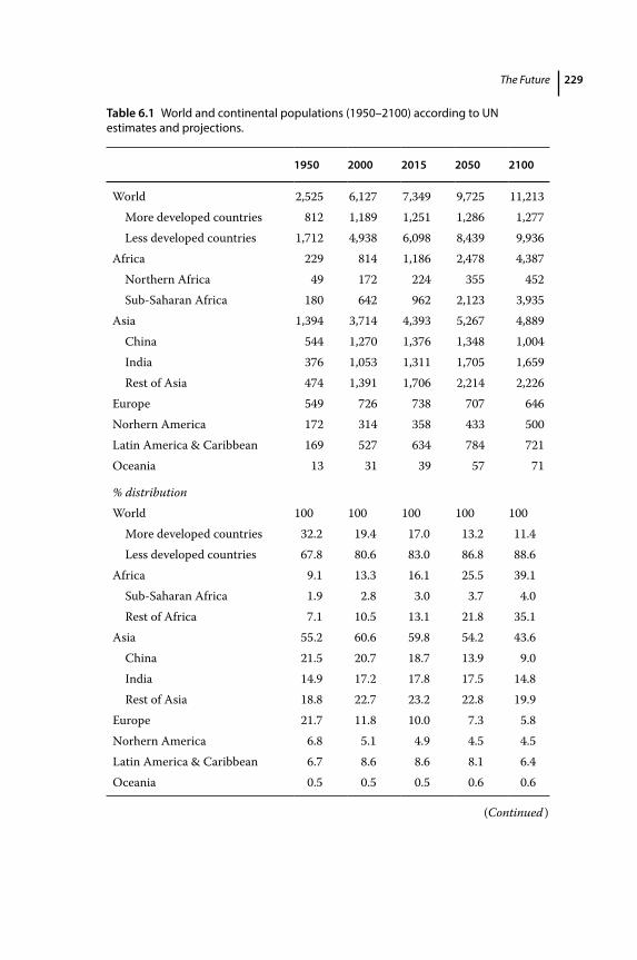
The Future 229
Table 6.1 World and continental populations (1950–2100) according to UN estimates and projections.
1950 2000 2015 2050 2100
World 2,525 6,127 7,349 9,725 11,213More developed countries 812 1,189 1,251 1,286 1,277Less developed countries 1,712 4,938 6,098 8,439 9,936
Africa 229 814 1,186 2,478 4,387Northern Africa 49 172 224 355 452Sub‐Saharan Africa 180 642 962 2,123 3,935
Asia 1,394 3,714 4,393 5,267 4,889China 544 1,270 1,376 1,348 1,004India 376 1,053 1,311 1,705 1,659Rest of Asia 474 1,391 1,706 2,214 2,226
Europe 549 726 738 707 646Norhern America 172 314 358 433 500Latin America & Caribbean 169 527 634 784 721Oceania 13 31 39 57 71
% distributionWorld 100 100 100 100 100
More developed countries 32.2 19.4 17.0 13.2 11.4Less developed countries 67.8 80.6 83.0 86.8 88.6
Africa 9.1 13.3 16.1 25.5 39.1Sub‐Saharan Africa 1.9 2.8 3.0 3.7 4.0Rest of Africa 7.1 10.5 13.1 21.8 35.1
Asia 55.2 60.6 59.8 54.2 43.6China 21.5 20.7 18.7 13.9 9.0India 14.9 17.2 17.8 17.5 14.8Rest of Asia 18.8 22.7 23.2 22.8 19.9
Europe 21.7 11.8 10.0 7.3 5.8Norhern America 6.8 5.1 4.9 4.5 4.5Latin America & Caribbean 6.7 8.6 8.6 8.1 6.4Oceania 0.5 0.5 0.5 0.6 0.6
(Continued )
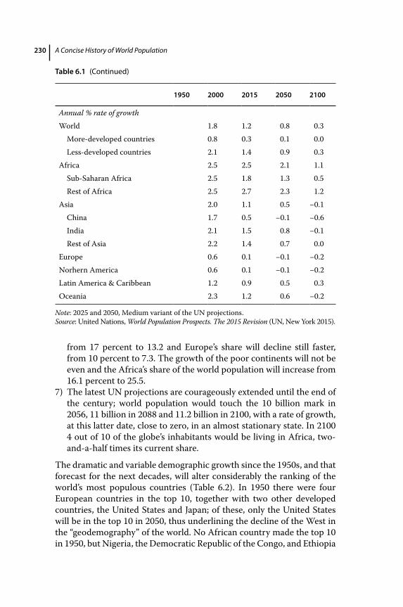
A Concise History of World Population230
from 17 percent to 13.2 and Europe’s share will decline still faster, from 10 percent to 7.3. The growth of the poor continents will not be even and the Africa’s share of the world population will increase from 16.1 percent to 25.5.
7) The latest UN projections are courageously extended until the end of the century; world population would touch the 10 billion mark in 2056, 11 billion in 2088 and 11.2 billion in 2100, with a rate of growth, at this latter date, close to zero, in an almost stationary state. In 2100 4 out of 10 of the globe’s inhabitants would be living in Africa, two‐and‐a‐half times its current share.
The dramatic and variable demographic growth since the 1950s, and that forecast for the next decades, will alter considerably the ranking of the world’s most populous countries (Table 6.2). In 1950 there were four European countries in the top 10, together with two other developed countries, the United States and Japan; of these, only the United States will be in the top 10 in 2050, thus underlining the decline of the West in the “geodemography” of the world. No African country made the top 10 in 1950, but Nigeria, the Democratic Republic of the Congo, and Ethiopia
1950 2000 2015 2050 2100
Annual % rate of growthWorld 1.8 1.2 0.8 0.3
More‐developed countries 0.8 0.3 0.1 0.0Less‐developed countries 2.1 1.4 0.9 0.3
Africa 2.5 2.5 2.1 1.1Sub‐Saharan Africa 2.5 1.8 1.3 0.5Rest of Africa 2.5 2.7 2.3 1.2
Asia 2.0 1.1 0.5 −0.1China 1.7 0.5 −0.1 −0.6India 2.1 1.5 0.8 −0.1Rest of Asia 2.2 1.4 0.7 0.0
Europe 0.6 0.1 −0.1 −0.2Norhern America 0.6 0.1 −0.1 −0.2Latin America & Caribbean 1.2 0.9 0.5 0.3Oceania 2.3 1.2 0.6 −0.2
Note: 2025 and 2050, Medium variant of the UN projections.Source: United Nations, World Population Prospects. The 2015 Revision (UN, New York 2015).
Table 6.1 (Continued)
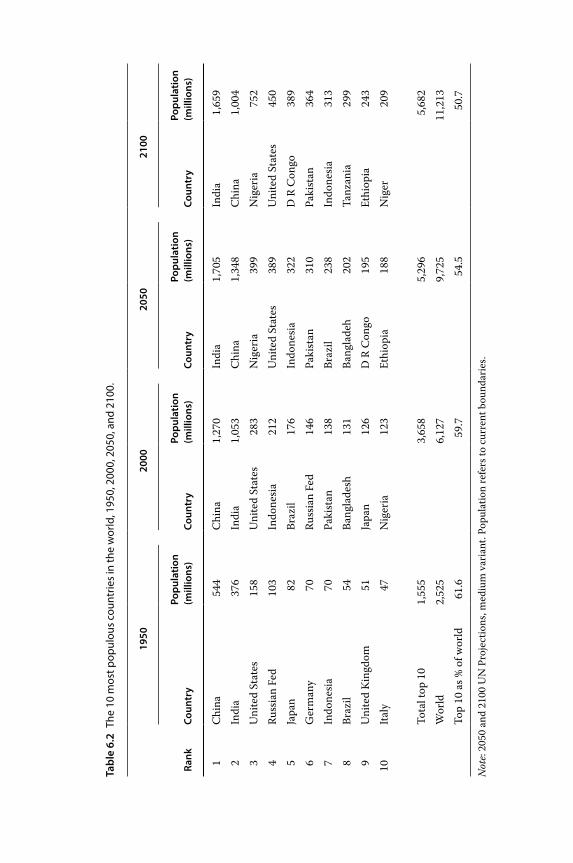
Tabl
e 6.
2 Th
e 10
mos
t pop
ulou
s co
untr
ies
in th
e w
orld
, 195
0, 2
000,
205
0, a
nd 2
100.
1950
2000
2050
2100
Rank
Coun
try
Popu
latio
n(m
illio
ns)
Coun
try
Popu
latio
n(m
illio
ns)
Coun
try
Popu
latio
n(m
illio
ns)
Coun
try
Popu
latio
n(m
illio
ns)
1C
hina
544
Chi
na1,
270
Indi
a1,
705
Indi
a1,
659
2In
dia
376
Indi
a1,
053
Chi
na1,
348
Chi
na1,
004
3U
nite
d St
ates
158
Uni
ted
Stat
es28
3N
iger
ia39
9N
iger
ia75
2 4
Russ
ian
Fed
103
Indo
nesi
a21
2U
nite
d St
ates
389
Uni
ted
Stat
es45
0 5
Japa
n82
Braz
il17
6In
done
sia
322
D R
Con
go38
9 6
Ger
man
y70
Russ
ian
Fed
146
Paki
stan
310
Paki
stan
364
7In
done
sia
70Pa
kist
an13
8Br
azil
238
Indo
nesi
a31
3 8
Braz
il54
Bang
lade
sh13
1Ba
ngla
deh
202
Tanz
ania
299
9U
nite
d K
ingd
om51
Japa
n12
6D
R C
ongo
195
Ethi
opia
243
10Ita
ly47
Nig
eria
123
Ethi
opia
188
Nig
er20
9
Tota
l top
10
1,55
53,
658
5,29
65,
682
Wor
ld2,
525
6,12
79,
725
11,2
13To
p 10
as %
of w
orld
61.6
59.7
54.5
50.7
Not
e: 20
50 a
nd 2
100
UN
Pro
ject
ions
, med
ium
var
iant
. Pop
ulat
ion
refe
rs to
cur
rent
bou
ndar
ies.
A Concise History of World Population232
will join the league of the most populous nations in 2050. Pakistan, ranking only thirteenth in 1950, will be in fifth place in 2050 while, in that year, India will have displaced China as the largest country of the world.
As a result of the variable dynamic of world nations, quantitative ratios between populations traditionally in conflict, or simply in contact, will change. And though relations between countries are conditioned primarily by political, cultural, and economic factors, major changes in their relative population sizes are bound to have an effect.5 For example, the Rio Grande separates the rich world of North America from the poor world of Mexico and Central America. The population ratio between these two areas was 4.6:1 in 1950; in 2050 it will be 2.1:1. It is hard to imagine that nothing will change as a result of this fact alone. The rich countries on the northern shore of the Mediterranean numbered 2.1 times the population of the poor countries on the southern and eastern shores in 1950; by 2050 this ratio will be 0.4:1. Surely it would not be surprising if this reversal carried some consequences with it? Indeed, the ongoing unrest is also a consequence of the demographic transformation. And what of the changing numerical relationships between countries traditionally in competition or in conflict and growing at d ifferent rates: Turkey and Greece, Brazil and Argentina, Israel and the nearby Arab countries (or the Arab population within its borders), not to mention China and India?
Projecting population into the future implies the adoption of a set of hypotheses concerning fertility, survival, and migration for the coming decades. The main assumption guiding the UN projections is one of “convergence” of behaviors among the different countries: fertility will fall where it is too high and rise where it is too low; survival will improve everywhere, but with a slower pace where life expectancy is high and a faster pace where it is low; migration rates will gradually fall both in sending and receiving countries. It is possible, with an appropriate technique, to “decompose” population change between 2010 and 2050 into four components: fertility, mortality, migration, and the initial age structure (or momentum). The contribution of fertility is obtained calculating what the population would be in the year 2050 if mortality remained fixed at the 2010 levels and net migration equaled zero. The contribution of mortality (fertility remains fixed at the 2010 level, and migration equal to zero) is calculated in a similar way. Finally, the contribution of the initial (2010) age structure (called also “inertia” or “momentum” of the population), is calculated setting the fertility level from 2010 to 2050 at replacement level and assuming that mortality remains fixed throughout the period at the 2010 level, and net migration equals zero. “Quantifying the roles of the demographic drivers of future population trends is important for developing policies and programmes aimed at balancing
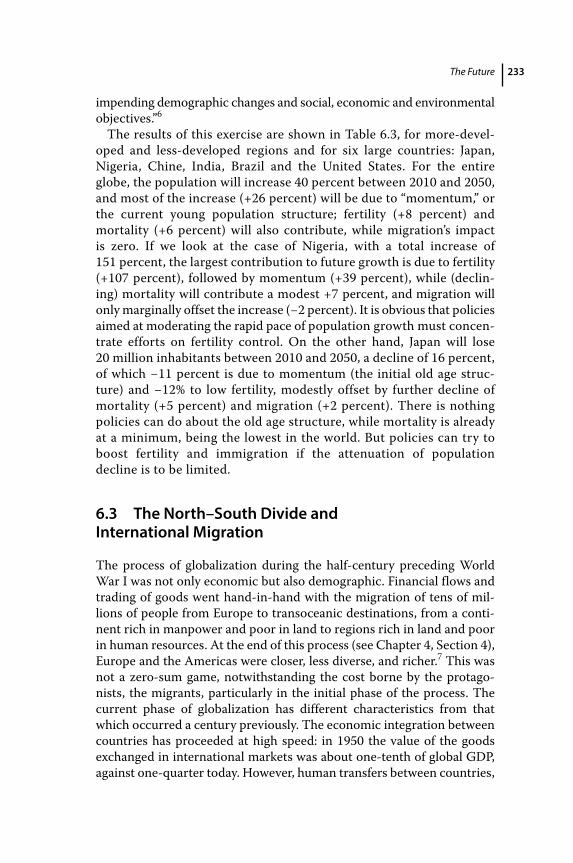
The Future 233
impending demographic changes and social, economic and environmental objectives.”6
The results of this exercise are shown in Table 6.3, for more‐developed and less‐developed regions and for six large countries: Japan, Nigeria, Chine, India, Brazil and the United States. For the entire globe, the population will increase 40 percent between 2010 and 2050, and most of the increase (+26 percent) will be due to “momentum,” or the current young population structure; fertility (+8 percent) and mortality (+6 percent) will also contribute, while migration’s impact is zero. If we look at the case of Nigeria, with a total increase of 151 percent, the largest contribution to future growth is due to fertility (+107 percent), followed by momentum (+39 percent), while (declining) mortality will contribute a modest +7 percent, and migration will only marginally offset the increase (−2 percent). It is obvious that policies aimed at moderating the rapid pace of population growth must concentrate efforts on fertility control. On the other hand, Japan will lose 20 million inhabitants between 2010 and 2050, a decline of 16 percent, of which −11 percent is due to momentum (the initial old age structure) and −12% to low fertility, modestly offset by further decline of mortality (+5 percent) and migration (+2 percent). There is nothing policies can do about the old age structure, while mortality is already at a minimum, being the lowest in the world. But policies can try to boost fertility and immigration if the attenuation of population decline is to be limited.
6.3 The North–South Divide and International Migration
The process of globalization during the half‐century preceding World War I was not only economic but also demographic. Financial flows and trading of goods went hand‐in‐hand with the migration of tens of millions of people from Europe to transoceanic destinations, from a continent rich in manpower and poor in land to regions rich in land and poor in human resources. At the end of this process (see Chapter 4, Section 4), Europe and the Americas were closer, less diverse, and richer.7 This was not a zero‐sum game, notwithstanding the cost borne by the protagonists, the migrants, particularly in the initial phase of the process. The current phase of globalization has different characteristics from that which occurred a century previously. The economic integration between countries has proceeded at high speed: in 1950 the value of the goods exchanged in international markets was about one‐tenth of global GDP, against one‐quarter today. However, human transfers between countries,
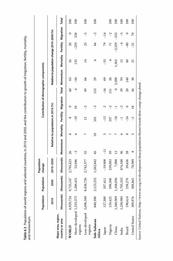
Tabl
e 6.
3 Po
pula
tion
of w
orld
regi
ons
and
sele
cted
cou
ntrie
s, in
201
0 an
d 20
50, a
nd th
e co
ntrii
butio
n to
gro
wth
of m
igra
tion,
fert
ility
, mor
talit
y,
and
mom
entu
m.
Maj
or a
rea,
regi
on,
coun
try
or a
rea
Popu
latio
nPo
pula
tion
Popu
latio
n ch
ange
Cont
ribu
tion
of d
emog
raph
ic c
ompo
nent
s
2010
2050
2010
–205
0Re
lativ
e to
pop
ulat
ion
in 2
010
(%)
Rela
tive
to p
opul
atio
n ch
ange
201
0–20
50 (%
)
(tho
usan
ds)
(tho
usan
ds)
(tho
usan
ds)
Mom
entu
mM
orta
lity
Fert
ility
Mig
ratio
nTo
tal
Mom
entu
mM
orta
lity
Fert
ility
Mig
ratio
nTo
tal
WO
RLD
6,92
9,72
49,
725,
147
2,79
5,42
326
68
040
6316
200
100
Mor
e‐de
velo
ped
regi
ons
1,23
3,37
51,
286,
421
53,0
46−2
6−1
010
4−4
413
5−2
2923
810
0
Less
‐dev
elop
ed
regi
ons
5,69
6,34
98,
438,
726
2,74
2,37
732
712
−249
6614
25−5
100
Sub‐
Saha
ran
Afr
ica
840,
390
2,12
3,23
21,
282,
842
4510
101
−315
329
666
−210
0
Japa
n12
7,30
010
7,41
1−1
9,90
8−1
15
−12
2−1
669
−33
79−1
4N
iger
ia15
9,42
539
8,50
823
9,08
339
710
7−2
151
264
71−2
100
Chi
na1,
340,
969
1,34
8,05
67,
088
127
−18
−10
2,30
01,
362
−3,3
29−2
3310
0In
dia
1,23
0,98
51,
705,
333
474,
348
366
−1−2
3993
15−4
−510
0Br
azil
198,
614
238,
270
39,6
5628
8−1
60
2014
040
−80
010
0U
nite
d St
ates
309,
876
388,
865
78,9
898
5−5
1826
3021
−21
7010
0
Sour
ce: U
nite
d N
atio
ns, h
ttp://
ww
w.un
.org
/en/
deve
lopm
ent/
desa
/pop
ulat
ion/
them
e/tr
ends
/dem
‐com
p‐ch
ange
.shtm
l.
The Future 235
regions, and continents are – in relative numbers – lower than they were in the previous phase of globalization. This may sound surprising in the face of the palpable migratory pressures that are developing in the poor world, of the growing absolute numbers of migrants, and of the many efforts that the rich world is making to contain the migratory pressures. The net migratory balance between the rich and the poor world was 0.6 million per year during the 1960s; it approximately doubled to 1.3 million per year in the 1970s and 1980s, grew to 2.5 million in the 1990s, and to 3.2 million in the first decade of the twenty‐first century (Table 6.4).8 This is indeed rapid growth: but also the world population has doubled during the same period. The United States, which at the beginning of the century had less than 100 million inhabitants, received in the 5 years preceding World War I a net immigration in excess of 1 million per year. There is another consideration to be made, concerning the fact that the population “transfer” from the poor to the rich countries has become a structural feature. Any population owes its renewal to the stream of n ewborn (biological renewal) and to the inflow of immigrants (social renewal). During the first decade of the twenty‐first century, in the rich countries, births have numbered 136 million and immigrants (net of repatriations) 32 million, for a total of 170 million “new” persons who constitute the positive component of societal renewal. In other words, migration has given a substantive contribution (one‐fifth in the last decade) to the rich countries’ renewal. Table 6.5 gives the estimates of the migratory stock in the various continents from 1960 to 2015. The stock of migrants in a given country is defined as the number of persons living in the country but born elsewhere or having foreign citizenship (one of the two criteria is used); the sum across countries gives the total world stock. This is only an approximation of the stock, since the definition of immigrant varies from country to country, and censuses, at the basis of these estimates, are a weak tool when used for counting migrants. World migratory stock has more than tripled between 1960 and 2015 (from 75.5 to 244 million), but owing to the rapid increase of the world population in the same period, the increase of the number of migrants per 100 inhabitants has been modest (2.5 percent in 1960 and 3.3 percent in 2015). The decline in migration in the developing world (from 2.1 p ercent to 1.7 percent) partially compensates for its tripling in the rich countries (from 3.4 to 11.4 percent). There are 32 migrants per 100 inhabitants in Saudi Arabia, 21 Oceania, 15 in North America, 10 in Europe, and only a fraction of 1 in China and India.
So complex is the migratory phenomenon that models and paradigms capture only part of its mechanisms; as a consequence predictions are extremely difficult to make. Flows and stocks are determined by the interaction of factors such as the differential growth of populations,
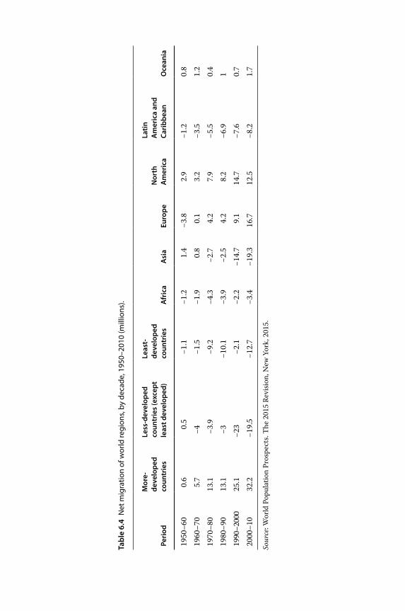
Tabl
e 6.
4 N
et m
igra
tion
of w
orld
regi
ons,
by d
ecad
e, 1
950–
2010
(mill
ions
).
Peri
od
Mor
e‐de
velo
ped
coun
trie
s
Less
‐dev
elop
ed
coun
trie
s (e
xcep
t le
ast d
evel
oped
)
Leas
t‐de
velo
ped
coun
trie
sA
fric
aA
sia
Euro
peN
orth
A
mer
ica
Latin
A
mer
ica
and
Cari
bbea
nO
cean
ia
1950
–60
0.6
0.5
−1.1
−1.2
1.4
−3.8
2.9
−1.2
0.8
1960
–70
5.7
−4−1
.5−1
.90.
80.
13.
2−3
.51.
219
70–8
013
.1−3
.9−9
.2−4
.3−2
.74.
27.
9−5
.50.
419
80–9
013
.1−3
−10.
1−3
.9−2
.54.
28.
2−6
.91
1990
–200
025
.1−2
3−2
.1−2
.2−1
4.7
9.1
14.7
−7.6
0.7
2000
–10
32.2
−19.
5−1
2.7
−3.4
−19.
316
.712
.5−8
.21.
7
Sour
ce: W
orld
Pop
ulat
ion
Pros
pect
s. Th
e 20
15 R
evis
ion,
New
Yor
k, 2
015.
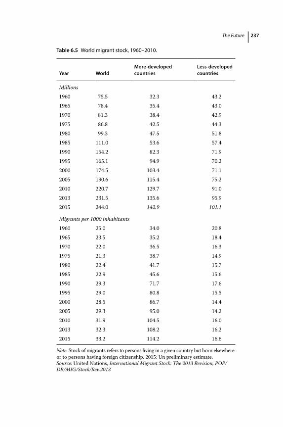
The Future 237
Table 6.5 World migrant stock, 1960–2010.
Year WorldMore‐developed countries
Less‐developed countries
Millions1960 75.5 32.3 43.21965 78.4 35.4 43.01970 81.3 38.4 42.91975 86.8 42.5 44.31980 99.3 47.5 51.81985 111.0 53.6 57.41990 154.2 82.3 71.91995 165.1 94.9 70.22000 174.5 103.4 71.12005 190.6 115.4 75.22010 220.7 129.7 91.02013 231.5 135.6 95.92015 244.0 142.9 101.1
Migrants per 1000 inhabitants1960 25.0 34.0 20.81965 23.5 35.2 18.41970 22.0 36.5 16.31975 21.3 38.7 14.91980 22.4 41.7 15.71985 22.9 45.6 15.61990 29.3 71.7 17.61995 29.0 80.8 15.52000 28.5 86.7 14.42005 29.3 95.0 14.22010 31.9 104.5 16.02013 32.3 108.2 16.22015 33.2 114.2 16.6
Note: Stock of migrants refers to persons living in a given country but born elsewhere or to persons having foreign citizenship. 2015: Un preliminary estimate.Source: United Nations, International Migrant Stock: The 2013 Revision, POP/DB/MIG/Stock/Rev.2013
A Concise History of World Population238
divergences in the standard of living, regulations and laws that influence migratory flows and their composition, proximity, and distance – in other words, demographic, economic, political, and geographic factors, not to speak of exceptional natural or political events. As far as the coming decades are concerned, some forces now in action will continue to d etermine future migratory flows with a strength that can be partially foreseen. We will discuss them in combination.
6.3.1 Demographic Inequalities
This subject has already been addressed: let us recall that the rate of increase of the population of active age will continue to diverge considerably in the rich and in the poor countries. In the rich countries, the very low birth rate of the past three or four decades has compressed growth, and ushered in a decline in the young age groups, even a sharp one in some countries. In the poor countries, on the other hand, the decline of the birth rate is a recent affair, and large numbers of young people will continue to enter the labor market for a long time. Between 2015 and 2050, the population aged 20 to 45 – an age group from which originates the great majority of migrants – will increase 22 percent in the poor countries, and decline 11 percent in the rich ones; the increase will be extraordinary in the sub‐Saharan region and the decline will be very p ronounced (between one‐fifth and one‐third) in large countries such as Japan, Russia, Germany, Italy, and Spain.
6.3.2 Economic Inequalities
If the trends of the past decades are a guide for the future, the gulf between the developing and the developed world is bound to widen. Between 1950 and 2000, the difference of GNI per capita (expressed in 1990 international dollars Geary‐Khamis) between the western economies (Europe and North America) on the one hand, and Asia, Africa, and Latin America on the other, has increased. In 1950, per capita income in Europe and North America was $4,000–$6,000 above the per capita income of each of the three continents; in the year 2010 the gap had widened to $16,000–$22,000. Even more surprising is the fact that during the period considered here not only have the absolute, but also the relative, differences increased: the ratio between GDP per capita in western economies and GNI per capita in Africa increased from 7:1 in 1950 to 12:1 in 2010, and in Latin America the same ratio increased from three to four; only in Asia has the relative gap narrowed, mainly owing to China’s and Japan’s performance.9
If these are the trends, are these gaps destined to increase in the future? Current growth is sustained by technological innovation, and there is an
The Future 239
enormous imbalance between the northern and southern hemispheres as far as production and possession of technology are concerned. The countries that are advanced in terms of scientific knowledge and technology innovation are also best placed to produce further innovation and know‐how, with a typical chain reaction, while the other areas stay behind. Only when the process of accumulation of scientific and technological innovation starts to abate – as happened in the first part of the twentieth century – will a process of diffusion accelerate and convergence take place. But this will take time; meanwhile it is likely that i nequalities between countries will continue to increase, as has happened in the past few decades.
6.3.3 Migration Policies
Migration policies are in continuous evolution, although some changes in direction can be seen. The first is the trend toward severe restrictions on the movement of refugees, which has reached the record number of 15 million in 2015. Asylum rights have been restricted in all countries, even those that have very liberal traditions, and the inflow of over a million refugees in Europe in 2015 has reinforced the trend. A second development consists of policies that tend to put in place more efficient barriers against illegal immigrants, making the borders less permeable, or tightening controls on illegal immigrants. Moreover, family reunification is made more difficult and more and more immigrant workers are selected on the basis of professional skills or other characteristics determined by the countries of immigration. If one had to venture a prophecy, policies seem oriented to more control, restriction, and selection.10
Notwithstanding the increasing stock of migrants, the integration among economies has proceeded much more rapidly than the interchange of peoples. The fact is that economic globalization has been sustained by a cultural and political action in favor of free trade and lower tariffs, and the setting up of a powerful regulating institution like the World Trade Organization (WTO). But barriers to migration, in the meantime, have been raised, and the action of global forces checked, for a time. No shared vision of common good has emerged and calls for international cooperation – not to say governance – have been feeble. It is a telling fact that few states have ratified the two ILO conventions (49 states for no. 97 of 1949 and only 23 for No. 143 of 1975) dealing explicitly with migrant workers, and that the United Nations Convention on the Rights of Migrant Workers and their Families needed 13 years to enter into force, and this – as of 2015 – has been ratified by only 48 states (only one in Europe). Too strong are the
A Concise History of World Population240
conflicting interests, too feeble the voice of migrants, too weak the p erception of common, long‐term interests.
The Global Commission on Migration and Development, created by the UN Secretary General, Kofi Annan, in 2003, after 2 years of consultation and debates, came up in 2005 with a rather timid proposal: the creation of an Inter‐Agency Global Migration Facility (IGMF) with the objective of facilitating a “coordinating and integrating policy planning in areas that cross the mandates of several institutions, for example human trafficking, the migration–asylum nexus and the developmental implications of international migration, including remittances.”11 In other words, the IGMF should coordinate functions that are carried out by various agencies (which would continue to carry out those functions), both belonging to the United Nations family – such as UNCHR or ILO – and outside the UN, like IOM, WTO. Areas of IGMF competence should include capacity building, policy planning and analysis, development, data collection, promoting consultation with regional bodies, NGOs, for example. But even this modest proposal for coordination of dispersed capacities and functions has remained unheeded. As for bringing together the “disparate migration‐related functions of existing UN and other agencies within a single organization,” this was left, in the Report, for a “long term approach,” meaning, by this, deferral to a far‐away n ebulous future.
If even minimalist proposals have been set aside, what about the idea of gradually building up a supranational institution – of the nature of the WTO – to which governments might cede parts (even minimal at the beginning) of their sovereignty in migration‐related issues? Proposals of this nature do not seem to be popular in the international debate and are left to the initiative of isolated voices.
The world badly needs enlightened immigration policies and best practices to be spread and codified. A World Migration Organization would begin to do that by juxtaposing each nation’s entry, exit and residence policies toward migrants, whether legal or illegal, economic or political, skilled or unskilled. Such a p roject is well worth putting at the center of policymakers’ concerns.12
Few voices have joined the debate. It is distressing to see that any reference to the governance of international migration is absent from the 17 Sustainable Development Goals and from the 169 related Targets s olemnly approved by the General Assembly of the United Nations in September 2015. The lack of even an embryo of international governance threatens the sustainability of development in the coming decades.
The Future 241
6.3.4 Geography and Migratory Systems
Notwithstanding the rapid process of globalization and the growth in numbers of migrants, migratory “systems” have remained unchanged over the second part of the twentieth century. By “system” we mean an area of attraction of centripetal migration flows originating from given geographical areas. Of these systems, we can identify three, or perhaps four, major ones: the system centered on North America and attracting people mainly from Latin America; the European system with a strong attraction for the countries of the south and west rims of the Mediterranean; a third system formed by the oil‐producing countries of the Persian Gulf attracting people from the Middle East. A fourth system has developed more recently, having at its center the fast‐growing economies of Southeast Asia. But vast regions of Africa, Asia, and Latin America have remained, for complex reasons, extraneous to migration processes. The break‐down of the Soviet Union and of its political and economic system did not bring about the east–west migration of millions of people, as had been prophesied after 1992. The fact that migratory systems had not extended significantly their areas of influence was also the consequence of the viscous inertia that ties the countries of origin and destination because of the numerous political, economic, and social connections that are being formed and strengthened over time, reinforced by the formation of large ethnic communities in the destination countries. New entries in the “system” were therefore more difficult. Concentration of the systems had also increased: in 1960 the migratory stock of the United States and Europe represented 39 percent of world stock; in 2000 its share had increased to 53 percent. In the first part of the current century, however, migration systems seem to enlarge their reach, and start including regions once outside their perimeter, as it is shown by the increasing presence in Europe of migrants coming from the sub‐Saharan region. Mobility is less costly, relations with the countries of origin need not to be severed, information circulates instantly; moreover, the deep demographic differentials and growing economic inequalities determine migratory tensions and pressures that the increasingly rigid migratory policies try to control and restrain. The result of these forces on the volumes of international migration is uncertain, even if the deep demographic deficit of a large part of the rich world implies a growing demand for immigration. The recent crisis has certainly checked the south–north migration push, but historical forces will resume once the economy goes back to normal.
6.3.5 Climate Change and Environment
One popular topic concerns the influence of climate change (See Chapter 6, Section 8) on migration, and the possible rise of waves of “environmental migrants” pushed out of drought‐hit regions or
A Concise History of World Population242
risk‐prone areas (low‐laying coastal zones) as a consequence of global warming. This question has been carefully examined by the International Panel on Climate Change (IPCC). Extreme weather episodes are expected to increase in frequency and intensity as a consequence of global warming and may become additional factors of migration. But “the evidence on displacement as a result of weather‐related events suggests that most displaced people attempt to return to their original residence and rebuild as soon as practical” as happened after the extensive Pakistan flood in 2010. History shows also that those pushed out by areas hit by long lasting droughts tend to return to their place of origin when the drought is over. In many cases of climate stressed situations, migration appears to be an adaptation of last resort.13 Given the uncertain course and intensity of global warming and the complexity of the factors that determine migration flows, it is impossible to make predictions on possible future flow of “environmental migrants.” On the other hand, humankind – as often argued in this book – is resilient and adaptable and it looks unlikely that climate change might become a major driver of dislocation and migration.
6.4 On Sustainability of Extended Survival
The results of the projections we have presented rely on assumptions shared by most experts in the field. Even prudent and realistic observers believe that a further increase in life expectancy is in store for the next generation or two, driven by the continuing decline of mortality at old ages; that major reversals are not plausible; that those levels of extended survival with improved health achieved at the beginning of the new century are not in danger; and that the gap between rich and poor populations will rapidly narrow.14 According to United Nations projections (medium variant), for instance, life expectancy (men and women) in developed countries has been calculated to increase further from about 78 years in 2010–15 to 83 in 2045–50, while the less‐developed countries would progress from 69 to 76. Large populations like Japan, France, Italy, and Spain are expected to be close to a life expectancy of 90 by the mid‐twenty‐first century. Indeed, during the twentieth century survival was extended almost continuously in the West and the same happened in the poor countries after World War II. Scientific knowledge has increased tremendously and so have the technical means of controlling disease. Basic living conditions have improved almost everywhere. Optimism appears justified when considering the future, and questions about the sustainability of current trends are seldom asked. Many believe that baby girls born at the beginning of this century will easily survive into the next,
The Future 243
with a life expectancy of 100 years. However, when dealing with the future one has to be aware that plausible forecasts have a degree of uncertainty and that the sustainability of current trends is threatened by a plurality of factors that may be labeled as biological, political, or economic. A discussion of these factors is important if we are to approach the future with a critical eye.15
6.4.1 Biological Sustainability
Nothing is fixed in the world of biology, since there is continuous interaction and mutual adaptation between the major players: humans (the object of our analysis), pathogenic microbes (bacteria, viruses, protozoa, spirochetes, rickettsia, etc.), or animals (reservoir or vectors of microbes). The historian has many proofs of the changing interactions between humans and pathogens, of the appearance of new diseases, the transformation of some, the disappearance of others. Plague, typhus, smallpox, syphilis, tuberculosis, malaria – all major scourges of the past – have come and gone, disappearing in one region and reemerging in another, with varying incidence and lethality.
Because of the relatively small amount of DNA or RNA, or both, that they carry, their rapid growth rate, and large populations, microbial pathogens can evolve and adapt very quickly. These evolutionary mechanisms allow them to adapt to new host cells or host species, produce “new” toxins, bypass or suppress inflammatory or immune responses, and develop resistance to drugs and antibodies. The ability to adapt is required for the successful competition and evolutionary survival of any microbial form, but it is particularly crucial for pathogens, which must cope with host defenses as well as microbial competition.16
Mutual interactions as well as behavioral and environmental modifications change the general picture continuously. In the 1950s and 1960s – in the wake of the success of antibiotics and other drugs – there were many hopes that infectious diseases could be eradicated for good. The insurgence, disappearance, and reemergence of many other diseases are either the consequence of the biological evolution of viruses and microbes, or of the interaction between the animal and the human world, or of the intrusion in isolated environments, or of the action – or neglect – of society. Influenza, yellow fever, encephalitis, AIDS, dengue, tularemia, Lyme disease, Lassa fever, Ebola, SARS, bird flu – all of these fall into one of the above‐cited categories. Other diseases that we believed vanquished in the 1950s and 1960s – like tuberculosis, malaria, or cholera – reemerge
A Concise History of World Population244
whenever environmental conditions deteriorate, and this may happen in urban slums as well as in impoverished rural areas.17
6.4.2 The AIDS Epidemic: Sustainable for the Rich, Unsustainable for the Poor
The HIV/AIDS infection was identified in 1981 and defined and named in 1982, but was already in the epidemic stage in central Africa in the 1970s, and there are proven traces of its appearance in the Congo as early as 1959. How the infection has developed among humans has yet to be proved beyond any possible doubt, but simian origin appears to be a plausible hypothesis. An infected person can transmit the virus to a healthy one through sexual contact or via blood (transfusions, needle sharing); pregnant women can infect their fetus and nursing mothers their babies. Once the infection is acquired it takes up to 10 years before a person develops AIDS, and once AIDS has developed (it is believed that all people infected will eventually progress to AIDS) death will follow, in most cases within 4 years from the manifestation of the first symptoms.18 This in the absence of the new antiretroviral drugs that have been developed recently.
The HIV/AIDS epidemic is a new disease and has spread all over the world, targeting the young and sexually active. Its dark image recalls the scourges of the past: deadly, like the plague; transmitted through sexual contact, like syphilis; affecting children and young adults, like smallpox; with a long incubation, like tuberculosis. While vaccines have not yet been developed, new expensive antiretroviral drugs (ART) lower infection of positive individuals and postpone the appearance of AIDS, thus extending their lives.
In Figure 6.1 the epidemic diffusion of HIV/AIDS is mapped; its epicenter is in equatorial central Africa (Rwanda, Uganda, Zambia, Congo) and the infection reaches Belgium and France through migratory contact with their former colonies. A stream of professional Haitians immigrated into Zaire after decolonization in the 1960s; among those who returned to Haiti, or migrated to the United States, were infected people who carried the disease to North America. From North America, Haiti, and the West Indies, the disease traveled to Central America and Brazil and spread to the rest of Latin America. Diffusion from central Africa to the south of the continent was fueled by wars and international trading and trucking routes and, in the case of South Africa, by the army returning from the war in Angola. International migration and international travel in a tight‐knit web of worldwide contacts has spread the disease all over the world.19
The epidemiology of HIV/AIDS in a given population depends on a series of factors, among which are the patterns of sexual behavior,
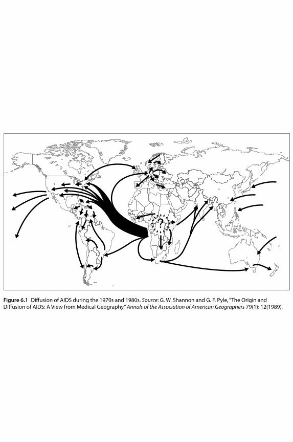
Figure 6.1 Diffusion of AIDS during the 1970s and 1980s. Source: G. W. Shannon and G. F. Pyle, “The Origin and Diffusion of AIDS: A View from Medical Geography,” Annals of the Association of American Geographers 79(1): 12(1989).
A Concise History of World Population246
the promiscuity and number of partners of infected females or males, and the state of health of the population at risk (particularly the frequency of venereal diseases and the presence of genital skin lesions). Infection among “sex workers” – males or females – is a powerful vehicle of diffusion. Patterns of male emigration out of rural villages into urban areas, multiple contacts with infected prostitutes, and periodic visits to the village of origin are conducive – as has happened in Africa – to a high rate of diffusion.20 When sexual transmission is largely among homosexuals, there is a high man‐to‐woman ratio among the infected; when transmission is mainly heterosexual the ratio – as in Africa – the ratio is close to one. Also, a high proportion of infected females means a high proportion of infected children.21
Table 6.6 portrays some features of the HIV/AIDS epidemic in 2014 according to official estimates. About 37 million people are believed to be infected worldwide, two‐thirds are in sub‐Saharan Africa. Prevalence rates in the adult population are generally a fraction of 1 percent, but they are over 1 percent in the Caribbean, and 5 percent in sub‐Saharan Africa. In this latter region, at the beginning of the millennium, prevalence exceeded 20 percent in South Africa and 30 percent in Zimbabwe and Botswana. In 1999, the results of a study that predicted that by 2003, in South Africa, AIDS‐related deaths would have exceeded deaths from all other causes combined, hit the headlines. The same study predicted that by 2009 life expectancy at birth – which had reached 61 in the early 1990s – would fall to 40.22 Ongoing developments are a little less tragic than those predicted as a consequence of the introduction of the new, efficient drugs, whose cost has decreased, but life expectancy still fell to 52 in 2005–10 (recovering to 58 in 2010–15). An extreme case is that of Botswana, where it is estimated that about one‐third of the adult population is infected with HIV, and where life expectancy declined from 63 in 1985–90 to 49 in 2000–5, a decline of 1 year for every calendar year. Predictions for the entire sub‐Saharan continent are currently less grim than they were a decade ago, thanks to the new therapies, to an increased awareness of the mechanisms underlying the transmission of the infection, to gradually changing lifestyles, and to the more active leadership of governments who, in the past, have been too slow to admit the tragic impact of the pandemic. The effects of this disaster go beyond demography: they affect culture, society, and the economy. Think of the rising proportion of orphans, left to the care of relatives or abandoned to their own devices; of the burden of a sick person, unable to work, on the family; of the burden of disease on society in terms of lost production and additional health costs. Only a few years ago, the current cost of life‐extending drugs for the total infected population would have exceeded the entire regional GDP.23 While waiting for efficient vaccines to be
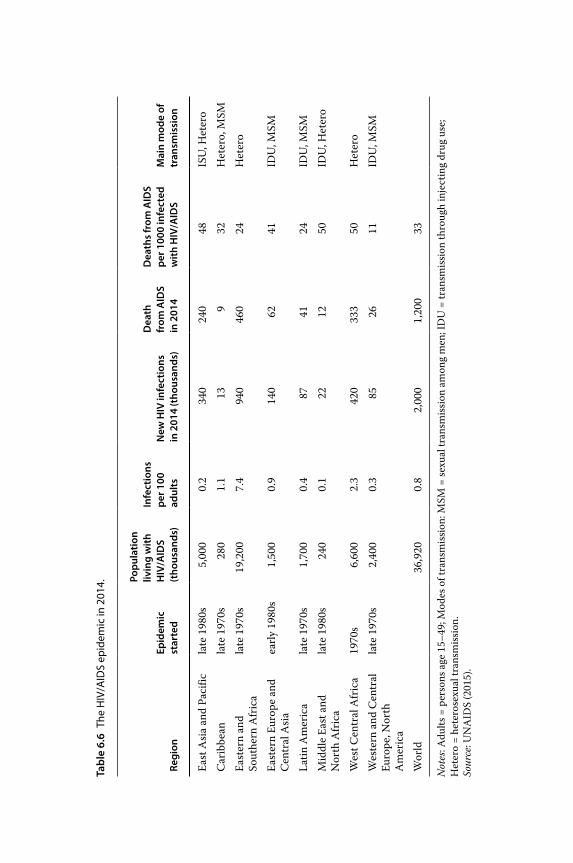
Tabl
e 6.
6 Th
e H
IV/A
IDS
epid
emic
in 2
014.
Regi
onEp
idem
ic
star
ted
Popu
latio
n liv
ing
with
H
IV/A
IDS
(tho
usan
ds)
Infe
ctio
ns
per 1
00
adul
tsN
ew H
IV in
fect
ions
in
201
4 (t
hous
ands
)
Dea
th
from
AID
S in
201
4
Dea
ths
from
AID
S pe
r 100
0 in
fect
ed
with
HIV
/AID
SM
ain
mod
e of
tr
ansm
issi
on
East
Asi
a an
d Pa
cific
late
198
0s5,
000
0.2
340
240
48IS
U, H
eter
oC
arib
bean
late
197
0s28
01.
113
932
Het
ero,
MSM
East
ern
and
Sout
hern
Afr
ica
late
197
0s19
,200
7.4
940
460
24H
eter
o
East
ern
Euro
pe a
nd
Cen
tral
Asi
aea
rly 1
980s
1,50
00.
914
062
41ID
U, M
SM
Latin
Am
eric
ala
te 1
970s
1,70
00.
487
4124
IDU
, MSM
Mid
dle
East
and
N
orth
Afr
ica
late
198
0s24
00.
122
1250
IDU
, Het
ero
Wes
t Cen
tral
Afr
ica
1970
s6,
600
2.3
420
333
50H
eter
oW
este
rn a
nd C
entr
al
Euro
pe, N
orth
A
mer
ica
late
197
0s2,
400
0.3
8526
11ID
U, M
SM
Wor
ld36
,920
0.8
2,00
01,
200
33
Not
es: A
dults
= p
erso
ns a
ge 1
5–49
; Mod
es o
f tra
nsm
issio
n: M
SM =
sexu
al tr
ansm
issio
n am
ong
men
; ID
U =
tran
smis
sion
thro
ugh
inje
ctin
g dr
ug u
se;
Het
ero
= he
tero
sexu
al tr
ansm
issio
n.So
urce
: UN
AID
S (2
015)
.
A Concise History of World Population248
developed, it is crucial that the international community develops the means and the ways to further lower the cost of the new therapies.
6.4.3 Political Sustainability
The second problem to be considered concerns the “political” sustainability of extended survival; the term political defines the broad institutional setting of society. Extended survival is not a simple achievement because it is the fruit of continuous incremental accumulation of scientific knowledge, of technological devices, of correct behaviors, of environmental safety, of material resources, and of efficient social action. This slow process is at the basis of progress as we knew it during the twentieth century. One must not forget that even at the end of the nineteenth century, in many European populations, and at the mid‐twentieth century in most developing societies, survival was no better than 1,000 years before. In the rich populations extension of survival was c ontinuous during the twentieth century, with only temporary and exceptional setbacks during the worst years of the two world wars.
Maintaining this pace of unrelenting progress during the next generation or two implies no major failure in the pillars that have sustained the progress achieved in the twentieth century. Yet history shows that this is not impossible: the case of the former Soviet Union is indeed macroscopic. What is now Russia had reached a life expectancy (both sexes combined) of 69 in the early 1960s, quite close to that of the western populations; then stagnation and a major setback followed and by the mid‐1990s life expectancy had fallen to 65, a decline of 4 years against an advance of about 7 years in western countries.24 The decline has been greater for the male population, whose life expectancy fell to 59 in 2000–5, returning to the levels of half a century before. The malfunction and then collapse of a political system is the general cause of the crisis of survival; levels of nutrition have declined; alcohol consumption has increased while product quality has deteriorated; public spending on health has fallen in real terms owing also to the increasing prices of drugs and high‐tech care; extreme poverty has skyrocketed, affecting almost one‐quarter of all households; a syndrome of social stress has developed and alcoholism, violence, and suicide have rapidly increased.25 Political collapse has produced an increase in mortality rates from cardiovascular and respiratory complaints, alcohol‐related diseases, violence, and so forth, particularly among adults. In a milder form, similar developments have taken place in other former socialist countries of central and eastern Europe.26 There are similar examples in developing countries: after the oil boom of the 1960s and early 1970s Nigeria suffered a period of political instability and impoverishment, with a deterioration of the health system.
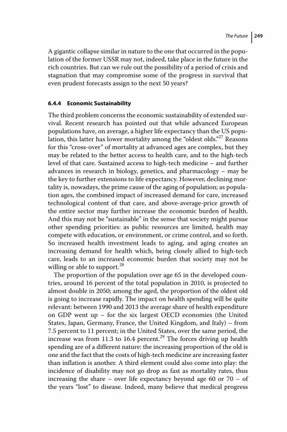
The Future 249
A gigantic collapse similar in nature to the one that occurred in the population of the former USSR may not, indeed, take place in the future in the rich countries. But can we rule out the possibility of a period of crisis and stagnation that may compromise some of the progress in survival that even prudent forecasts assign to the next 50 years?
6.4.4 Economic Sustainability
The third problem concerns the economic sustainability of extended survival. Recent research has pointed out that while advanced European populations have, on average, a higher life expectancy than the US population, this latter has lower mortality among the “oldest olds.”27 Reasons for this “cross‐over” of mortality at advanced ages are complex, but they may be related to the better access to health care, and to the high‐tech level of that care. Sustained access to high‐tech medicine – and further advances in research in biology, genetics, and pharmacology – may be the key to further extensions to life expectancy. However, declining mortality is, nowadays, the prime cause of the aging of population; as population ages, the combined impact of increased demand for care, increased technological content of that care, and above‐average‐price growth of the entire sector may further increase the economic burden of health. And this may not be “sustainable” in the sense that society might pursue other spending priorities: as public resources are limited, health may compete with education, or environment, or crime control, and so forth. So increased health investment leads to aging, and aging creates an increasing demand for health which, being closely allied to high‐tech care, leads to an increased economic burden that society may not be w illing or able to support.28
The proportion of the population over age 65 in the developed countries, around 16 percent of the total population in 2010, is projected to almost double in 2050; among the aged, the proportion of the oldest old is going to increase rapidly. The impact on health spending will be quite relevant: between 1990 and 2013 the average share of health expenditure on GDP went up – for the six largest OECD economies (the United States, Japan, Germany, France, the United Kingdom, and Italy) – from 7.5 percent to 11 percent; in the United States, over the same period, the increase was from 11.3 to 16.4 percent.29 The forces driving up health spending are of a different nature: the increasing proportion of the old is one and the fact that the costs of high‐tech medicine are increasing faster than inflation is another. A third element could also come into play: the incidence of disability may not go drop as fast as mortality rates, thus increasing the share – over life expectancy beyond age 60 or 70 – of the years “lost” to disease. Indeed, many believe that medical progress
A Concise History of World Population250
improves the survival of the frail who, however, are the victims of disabling conditions, thus raising the general incidence of old‐age disability. This area of study is quite new: comparisons across countries and over time are quite difficult, and trends are uncertain. The proportion of years lost to disease (or lived in poor health) seems to decrease in some countries and stagnate or even decrease in others, but the trends in disability will be important in determining the trends in health spending.30 Some interesting considerations can be gained from Figure 6.2, where health expenditure per capita is plotted against life expectancy in both rich and poor countries. Beyond certain levels of expenditure, life expectancy remains more or less the same, and this confirms what we stated earlier: immaterial factors that cannot be converted into monetary terms (knowledge, organization, best practices, behaviors) are relevant factors of human survival. What if health spending continues to go up? What will happen if health systems start cutting back on high‐tech treatment? Will low survival in old age continue to improve?
We were not created to be eternal, but if a miraculous drug of perennial life was discovered, and we wished to maintain the world population at the current level between 7 and 8 billion – which many view as already a too‐high and dense population – then no further births could be allowed on the planet. Extended survival must be compatible with our demographic and social systems; must be sustained by continuous control and surveillance of the biological world; guaranteed by political regimes that are reasonably stable and whose necessary changes do not entail the traumatic consequences that many societies endured in the twentieth century; and be based on a continuous stream of available resources for
0 1,000
Per capita expenditure on health (international $)
2,000 3,000 4,000 5,000 6,00030
40
50
60
Life
exp
ecta
ncy
at b
irth
(e0)
70
80
90
Figure 6.2 Per capita expenditure on health (international $) and life expectancy at birth (2002).
The Future 251
research, prevention, and cure. If the world population could extend its life expectancy during the twentieth century at the rate of 4 months per year, this heroic enterprise will not be possible in the twenty‐first century, whose more prosaic mission will be to maintain the gains achieved, extend them throughout the poor world, prevent reversals, and improve the quality of life.31
6.5 The Moving Limits
The latter part of the twenty‐first century will likely witness a population 50 percent larger than its present size. It is difficult, however, to say whether growth of this sort will jeopardize economic and social progress since, as repeatedly noted, population is not an “independent variable” but reacts and adapts to the possibilities for expansion that it encounters. In past centuries, many scholars have held firmly to the idea that there is a global “carrying capacity,” or in any case a maximum sustainable size, given the limits of space and technology and the need to maintain quality of life and avoid environmental decay. 32 One can of course debate at length the question of quality of life for, like Giammaria Ortes, we do not want to see humanity “grow not only beyond the number of persons that could breathe on the earth, but to such a number as could not be contained on all its surface, from lowest valley to highest mountain, crowded and crammed together like dried dead herrings in their barrel,”33 a condition that a certain type of technological progress might even make possible.
The identification of a “carrying capacity” presents so many conceptual difficulties as to be virtually useless for practical purposes. It is an idea derived from biology and animal ecology designed to measure the c apacity of a certain environment to sustain animal life. With the human species, however, we also need to take into account the development of technology, the elasticity of the concept of quality of life, and the ability to adapt and interact in a complex and not easily modeled dynamic s ystem. Nonetheless, we do live in a finite world, and the question of where we place the boundary beyond which numbers and resources enter into conflict is important. Figure 6.3, taken from Limits to Growth,34 describes four possible modes of interaction between population and “carrying capacity.” The first two modes (Figure 6.3a and Figure 6.3b) represent an optimistic view in which the two forces do not come into conflict. In the first case, as population grows so does carrying capacity (CP), thanks to technological progress, and the two curves do not intersect; in the second, CP is constant but population growth slows as it approaches the limit imposed by the finite environment. The other two
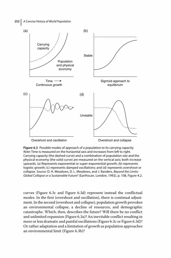
A Concise History of World Population252
curves (Figure 6.3c and Figure 6.3d) represent instead the conflictual modes. In the first (overshoot and oscillation), there is continual adjustment. In the second (overshoot and collapse), population growth provokes an environmental collapse, a decline of resources, and demographic catastrophe. Which, then, describes the future? Will there be no conflict and unlimited expansion (Figure 6.3a)? An inevitable conflict resulting in more or less dramatic and painful oscillations (Figure 6.3c or Figure 6.3d)? Or rather adaptation and a limitation of growth as population approaches an environmental limit (Figure 6.3b)?
Unstable
Overshoot and oscillation Overshoot and collapse
Sigmoid approach toequilibrium
TimeContinuous growth
Populationand physical
economy
Carryingcapacity
Stable
(b)(a)
(c) (d)
Figure 6.3 Possible modes of approach of a population to its carrying capacity. Note: Time is measured on the horizontal axis and increases from left to right. Carrying capacity (the dashed curve) and a combination of population size and the physical economy (the solid curve) are measured on the vertical axis; both increase upwards. (a) Represents exponential or super‐exponential growth; (b) represents logistic growth; (c) represents damped oscillations; and (d) represents overshoot or collapse. Source: D. H. Meadows, D. L. Meadows, and J. Randers, Beyond the Limits: Global Collapse or a Sustainable Future? (Earthscan, London, 1992), p. 108, Figure 4.2.
The Future 253
The attempt to estimate the earth’s carrying capacity is more than three centuries old. These estimates are based on a variety of criteria: from categorical and absolute pronouncements, to the adaptation and extrapolation of mathematical curves, to the extension of observed population densities to the entire terrestrial surface. Other methods rely on the availability of a limited resource, usually food, to calculate a maximum possible population; and yet others combine several limited resources, for example, food and water. The most complex efforts seek to simulate the interaction between various factors, their substitutability, and the adaptation of lifestyles. In 1995, Joel Cohen critically reviewed all the well‐known attempts to estimate carrying capacity,35 from the earliest estimates of the Dutchman Leeuwenhoek (1679), the Englishman Gregory King (1695), and the German Peter Sussmilch (1741 and 1765) – all within a relatively narrow range of between 4 and 13.9 b illion – to the most recent. Of the 93 estimates reviewed by Cohen, 17 give a carrying capacity below 5 billion; 28 between 5 and 10 billion; 16 between 10 and 15 billion; 8 between 15 and 25 billion; 13 between 25 and 50 billion; and 11 over 50 billion.36 The median is around 10 billion, a level that should be reached in 2056 according to the projections used in this book. The differences depend on both the methods and the hypotheses used. Surprisingly, however, the “ceiling” does not increase as one moves from older to more recent estimates; instead it is the variability of the estimates that increases. But these figures are little more than statistics of statistics, good for satisfying one’s curiosity but not much of a guide to the real carrying capacity of the earth.
Looking ahead to the future from our own vantage point of the present day, more recent estimates that take into account technological change and lifestyles and which are informed by contemporary and less hypothetical situations are of greater interest. A few merit our immediate consideration. One of the highest carrying capacities was calculated by De Wit (1967) on the supposition that the process of photosynthesis would be the limiting factor and that neither water nor mineral resources would impose limits.37 He divides an estimate of the productive potential of carbohydrates per hectare of cultivable land available in the various climatic regions of the world by per capita caloric consumption to come up with an estimated carrying capacity per hectare, and so a maximum population, should all possible land be devoted to cultivation (first s ubtracting, for each individual, a certain area for home, work, transportation, recreation, and so on). In this way, he comes up with a maximum figure of 146 billion, allowing 750 m2 of nonproductive land per person, or else 73 billion, allowing a double quota of 1,500 m2. Colin Clark (1967 and 1977) obtained similar results by different means: estimating the surface area needed per person to feed and supply basic needs, he has come up with a maximum figure of
A Concise History of World Population254
157 billion assuming Japanese levels of consumption (at the time), and a minimum of 47 billion assuming North American levels.38 Roger Revelle instead has derived a lower estimate by multiplying available cultivable area (not including wet tropical areas and land needed for nonfood production) by the productivity achievable with irrigation and present‐day advanced technology to arrive at a carrying capacity of 40 billion.39
These estimates are all on the high end of the scale and rely on some difficult assumptions (for example, that all available land be cultivated with advanced techniques). By introducing more realistic hypotheses, the estimates rapidly decrease. Gilland (1983), for example, has employed a method similar to Revelle’s but using less optimistic estimates with regard to cultivable area and productivity, and derives a much lower estimate of 7.5 billion at comfortable levels of consumption.40 A joint FAO–IIASA (1983) study takes a different approach. Based on a map of soil types prepared by the FAO (and including all the developing world except China), various climatic regions were studied in relation to 15 basic crops and estimates of productive potential were arrived at according to three different hypotheses.41 The low hypothesis envisions unchanging cultivation and traditional methods employed without fertilizer, pesticides, or mechanization, while the high one foresees employment of the gamut of green‐revolution technology including full mechanization and use of pesticides and fertilizers. The middle hypothesis makes more realistic assumptions. The carrying capacity of this area, which had a population of about 2 billion in 1975, was put at 4 billion (level reached in 2010) according to the low hypothesis, 13.7 according to the intermediate, and 32.8 according to the high. A balanced study by Smil (1994) concluded that a realistic reduction in the inefficiencies, irrationality, and waste in the production, distribution, and consumption system could make possible the survival of another 2.5–3 billion people at current levels of consumption, and that additional productive inputs – leaving aside the possibility of revolutionary developments in bioengineering – could feed another 2–2.5 billion.42 From another perspective, sociobiologist Edward O. Wilson wrote: “If everyone agreed to become vegetarian, leaving little or nothing for livestock, the present 1.4 billion hectares of arable land (3.5 billion acres) would support about 10 billion people.”43 It seems, then, realistic to think that the earth will be able to sustain 10 or 11 billion people during the twenty‐first century. There are of course more restrictive hypotheses that incorporate higher levels of consumption and strict measures of conservation and environmental management and which estimate carrying capacities below the present‐day population. The fact, however, that those limits have been exceeded in the context of declining real prices, as we will see later on, increasing average levels of health, life expectancy, and well‐being casts them in some doubt.
The Future 255
The question of the limits to growth and of a fixed population level compatible with the carrying capacity of the planet is an elusive one. Human behavior interacts in a dynamic and often unpredictable way with the external constraints. Limits may move forward, but also backward. Moreover, if we take into consideration a larger context that includes not only the availability of a certain quantity of goods per person but also lifestyles, quality of the environment, availability of space, and all those things that are valued in a particular historical and cultural period, then the problem becomes much more complicated. In fact it becomes insoluble, for there is a legitimate and ultimately unbridgeable philosophical gap between those who believe in the need for the greatest p ossible availability of open space and of silence and those instead who favor lifestyles closely linked to large and dense populations.
Let us now go back to the fact that several billion people – about four if we accept the reasonable UN projections – will accrue to today’s world population before the end of this century. In the next three sections we will explore how this growth will impact on the major constraints that humankind will have to face in the coming decades. Three domains will be considered and discussed. The first is the inevitable growth of the consumption of nonrenewable resources over the coming decades and, therefore, the nonsustainability of development for a more or less long period. The second is the impact of population growth on the demand for food; the third concerns the changing allocation of space, with particular emphasis on fragile environments and the contribution of population growth to atmospheric pollution and so to global warming. More population – and with it a greater degree of affluence – will imply more consumption, an intensification of human activity, an accrued impact on the environment. Women and men will have to respond with the qualities with which they have been endowed since time immemorial: adaptability, flexible behavior, ingenuity, innovation.
6.6 Non‐Renewable Resources and the Parable of Pauperia and Tycoonia
Let us examine the first point. It is well known that the per capita levels of consumption of commodities and energy for the rich economies are several times those for the poor ones. According to estimates of the 1990s, the ratio was 20 times higher for aluminum consumption, 17 times higher for copper, 10 times higher for iron ore, nine times higher for fossil fuel, and three times higher for roundwood, just to give a few examples.44 Estimates of the extraction (metric tons per capita per year) of material resources such as ores and industrial minerals, fuel and energy carriers,
A Concise History of World Population256
construction minerals, and biomasses provide a synthetic measure. In developed countries the total extraction, in the year 2000, was 20 tons per capita, more than triple the extraction in developing countries.45 Rich countries, then, contribute disproportionately to the depletion of resource reserves. However, the future outlook for the rich countries is less bleak than the present situation because substitution, recycling, and changes in consumption patterns may determine a decline in the energy and commodity content of each additional dollar’s worth of production.46 Moreover, the rich populations will grow slowly or not at all in future decades. Therefore, prospects for the stabilization or even decline over the long run of the consumption of basic resources in the rich countries have some foundation. Prospects for the poor countries are different. According to World Bank estimates for 201447 the per capita GNI of the poor economies (defined as “low” or “middle” income and representing 85 percent of the world population) was $4.238 as compared to $38,274 for the rich economies (“high” income). Growth over the next decades of the poor economies will have to exceed that of the rich ones if the ratio (if not the absolute gap) between the affluence of the two worlds is to be reduced. Over the next generation the per capita GNI of these economies will have to be multiplied by a factor of two, three, or more, which will imply more iron and minerals for tools, more fiber for clothing, more wood for building, more food for nutrition, more space for living, and more energy for all these activities. Since the standard of living of the poor populations is very low, this additional stream of goods per person will have to be obtained with high inputs of energy, commodities, and space for each dollar’s worth of production. And these populations are of course asking for more food, tools, clothing, houses, and fuel. Considering that over the next two generations many of the poorest countries will double or triple in size and that the stream of per capita goods will have to be multiplied several times, it is easy to understand that this indispensable growth will hardly be sustainable for a very long time.48 This is the logic of the so‐called “environmental Kuznets curve” (based on the intuition of the economist Simon Kuznets in the 1950s), according to which, as income increases, the energy and material content of each production unit also increases but at declining rates, until a turning point is reached, after which the same rate becomes negative and the material content of additional production units declines. The curve is, therefore, bell shaped. In the long run, today’s poor countries could follow the same bell‐shaped curve and reduce the material content of each unit of production and consumption, as is now happening (at least for some manufactured goods) in high‐income countries.49 However, this will be a gradual and slow process and several generations will pass before this process – in conjunction with a stationary world population – leads to the arrest of
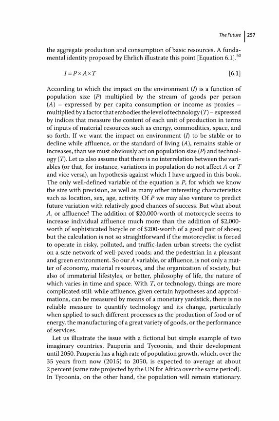
The Future 257
the aggregate production and consumption of basic resources. A fundamental identity proposed by Ehrlich illustrate this point [Equation 6.1].50
I P A T [6.1]
According to which the impact on the environment (I) is a function of population size (P) multiplied by the stream of goods per person (A) – expressed by per capita consumption or income as proxies – multiplied by a factor that embodies the level of technology (T) – expressed by indices that measure the content of each unit of production in terms of inputs of material resources such as energy, commodities, space, and so forth. If we want the impact on environment (I) to be stable or to decline while affluence, or the standard of living (A), remains stable or increases, than we must obviously act on population size (P) and technology (T). Let us also assume that there is no interrelation between the variables (or that, for instance, variations in population do not affect A or T and vice versa), an hypothesis against which I have argued in this book. The only well‐defined variable of the equation is P, for which we know the size with precision, as well as many other interesting characteristics such as location, sex, age, activity. Of P we may also venture to predict future variation with relatively good chances of success. But what about A, or affluence? The addition of $20,000‐worth of motorcycle seems to increase individual affluence much more than the addition of $2,000‐worth of sophisticated bicycle or of $200‐worth of a good pair of shoes; but the calculation is not so straightforward if the motorcyclist is forced to operate in risky, polluted, and traffic‐laden urban streets; the cyclist on a safe network of well‐paved roads; and the pedestrian in a pleasant and green environment. So our A variable, or affluence, is not only a matter of economy, material resources, and the organization of society, but also of immaterial lifestyles, or better, philosophy of life, the nature of which varies in time and space. With T, or technology, things are more complicated still: while affluence, given certain hypotheses and approximations, can be measured by means of a monetary yardstick, there is no reliable measure to quantify technology and its change, particularly when applied to such different processes as the production of food or of energy, the manufacturing of a great variety of goods, or the performance of services.
Let us illustrate the issue with a fictional but simple example of two imaginary countries, Pauperia and Tycoonia, and their development until 2050. Pauperia has a high rate of population growth, which, over the 35 years from now (2015) to 2050, is expected to average at about 2 p ercent (same rate projected by the UN for Africa over the same period). In Tycoonia, on the other hand, the population will remain stationary.
A Concise History of World Population258
Pauperia, enjoys a relatively high rate of growth of 5 percent of its per‐capita income and experts affirm that this rate is economically sustainable throughout the period under consideration. Tycoonia, however, will enjoy a much lower rate, estimated at 2 percent. Since the physical impact of mankind on Earth is a function of the combination of population and economic affluence (or income or product), P × A of Ehrlich’s equation [6.1], a simple multiplicative algorithm tells us that, over the next 35 years, such impact (assuming business as usual) would double in Tycoonia, but would increase more than 12‐fold in Pauperia. We all know that more technology may “decouple” economic growth from unsustainable patterns of production and consumption. In other words, with more technology it is possible to lower the content of energy and nonrenewable materials of every additional unit produced or consumed. This may easily happen in Tycoonia, where the dematerialization of c onsumption is possible (an additional dollar may be spent on buying an ebook, enjoying a concert, purchasing a haircut), but much less so in Pauperia, where an additional dollar is spent on buying gasoil for heating, cooking, and transportation; metal tools for work; food for nutrition; shoes for walking; and other basic commodities for which dematerialization is impossible or minimal. This example shows how, in poor societies, the impact of population and economic growth on the environment is going to be very heavy, unsustainable one would be tempted to say, in the coming decades. Hence we can identify two general priorities: the first is an acceleration of technological innovation (transferred from the rich countries or, better, produced locally) in the poor world and the second consists of reducing the speed of population growth. If fertility remained unchanged (at the current TFR level of 5.1) over the next 35 years, the population of Sub‐Saharan Africa would triple between 2015 and 2050 (from 0.96 to 2.75 billion). If TFR declined to 2.7 by 2050 (as assumed by the medium variant of the UN projections) population would “only” double (from 0.96 to 1.92 billion). It is a brutal calculation, but a one point difference of TFR in 2050 corresponds to approximately 350 million fewer people at that date. Fertility decline must remain a priority central to the sustainable development discourse. On the other hand, improving the human capital of the population (including the enhancement of its demographic component) will set the ground for responding to the second priority, the acceleration of technological transfers.
A final question needs some clarification. Given the expected population growth before the end of the century, are we going to run into a growing scarcity of nonrenewable resources that will slow or reverse development and affect the standard of living? Will the scarcity of nonrenewable resources act as a Malthusian check, as the Club of Rome
The Future 259
movement predicted in the 1970s? In a similar vein the economist Jevons, at the end of the nineteenth century, feared that a scarcity of coal would compromise industrial production. There are indications that we may not run up against these limits any time soon, and for three closely linked reasons. The first is that the ratio between reserves (not potential reserves but those that can be profitably extracted at current prices) and production (the reserve‐to‐production ratio, or reserve‐life index) does not show an increasing trend for the major minerals.51 Secondly, as can be seen in Figure 6.4, the real prices of primary resources have declined over the past 100 years, in spite of the growth of population and production. And thirdly, technological innovation determines a high level of substitution for nonrenewable resources. As one or another mineral becomes scarce, prices increase and so encourage the development of new technology to allow for this sort of substitution. These general considerations are valid only at the macro and planetary levels. Differences in development, natural resources, political institutions, and natural or human‐made disasters do not allow us to extend the same sort of discussion to local or regional levels.
6.7 Food for All?
Population growth impacts agriculture and the demand for food, and so also land use and other natural resources. This is the second of the three critical aspects of the population‐environment link. Over the next 35 years (2015–50), world population will increase by one‐third; this growth will imply at least a proportional increase in the production of food – but much more if the general standard of living has to be raised, food security increased, and the number of the undernourished, estimated in 2015 at
801910 1920 1930 1940 1950 1960 1970 1980 2000 2010
Index 2000 = 100
100
120
140
160
180
200
Figure 6.4 Composite resources price index at constant prices, 1900–2000. Source: UNEP, Decoupling Natural Resource Use and Environmental Impact from Economic Growth (UNEP, 2011), Figure 2.4, p. 13.
A Concise History of World Population260
800 million, reduced.52 According to FAO estimates it looks likely that the increased demand in the coming decades will be satisfied.53 About four‐fifths of total consumption consists of grains, so that the increased demand for grains (together with demand for other foods, fibers, and fuel).
will add enormously to pressure on natural resources – not only on agricultural land but also on stocks of water, fish, and timber. Natural resources will have to be managed with great care. They will need protection from the inadequate stewardship that is the consequence of poverty, population pressure, ignorance, and corruption. Natural forests, wetlands, coastal areas, and grasslands – all of high ecological value – will have to be protected from overuse and degradation.54
This assessment of the World Bank, a quarter of a century ago, is still valid today. Past trends suggest the options for the future: Figure 6.5 shows the trend over the past 50 years of the production of cereals (more than tripled), of the inputs of fertilizers (increased ninefold), and of the surface of cultivated land (unchanged). Of course, the same options are open for the future: grain production may be obtained either by adding new land to cultivation or through an intensification of already cultivated areas. Both options have different potential impacts on the environment; citing the World Bank:
If more food can be grown on the same land, that will ease pressure to cultivate new land and will permit the preservation of intact natural areas … But intensification can also produce problems. Raising yields by increasing the use of chemicals, diverting more water for irrigation, and changing land use can create problems elsewhere. Runoff of fertilizer and animal wastes can cause algal blooms and the eutrophication of lakes, coastal estuaries, and enclosed seas. Although these externalities are more common in Western Europe and North America, pollution from agricultural sources is becoming significant in Eastern Europe and other parts of the developing world as well; in the Punjab in India and Pakistan and in Java, Indonesia, the use of chemical inputs is almost as great as in industrial areas.55
The alternative to intensification is bringing new areas under cultivation (extensification), but one does not need to quote Malthus to conclude that this process cannot go on forever; indeed in some countries – Bangladesh, for instance – the limits have already been reached. In the past two decades or so biotechnology has emerged as another way to
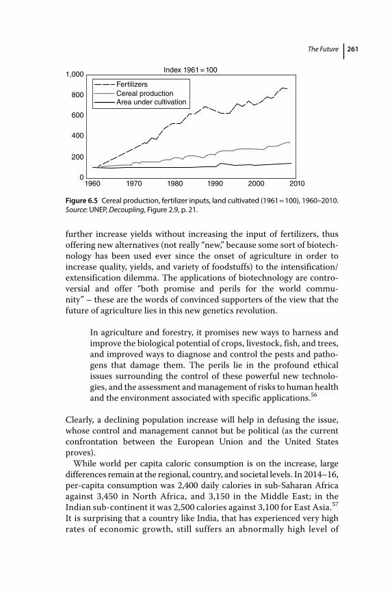
The Future 261
further increase yields without increasing the input of fertilizers, thus offering new alternatives (not really “new,” because some sort of biotechnology has been used ever since the onset of agriculture in order to increase quality, yields, and variety of foodstuffs) to the intensification/extensification dilemma. The applications of biotechnology are controversial and offer “both promise and perils for the world community” – these are the words of convinced supporters of the view that the future of agriculture lies in this new genetics revolution.
In agriculture and forestry, it promises new ways to harness and improve the biological potential of crops, livestock, fish, and trees, and improved ways to diagnose and control the pests and pathogens that damage them. The perils lie in the profound ethical issues surrounding the control of these powerful new technologies, and the assessment and management of risks to human health and the environment associated with specific applications.56
Clearly, a declining population increase will help in defusing the issue, whose control and management cannot but be political (as the current confrontation between the European Union and the United States proves).
While world per capita caloric consumption is on the increase, large differences remain at the regional, country, and societal levels. In 2014–16, per‐capita consumption was 2,400 daily calories in sub‐Saharan Africa against 3,450 in North Africa, and 3,150 in the Middle East; in the Indian sub‐continent it was 2,500 calories against 3,100 for East Asia.57 It is surprising that a country like India, that has experienced very high rates of economic growth, still suffers an abnormally high level of
FertilizersCereal production
1,000
0
200
400
600
800
1960 1970 1980 1990 2000 2010
Index 1961 = 100
Area under cultivation
Figure 6.5 Cereal production, fertilizer inputs, land cultivated (1961 = 100), 1960–2010. Source: UNEP, Decoupling, Figure 2.9, p. 21.
A Concise History of World Population262
malnutrition and undernutrition. In India, the incidence of children underweight is 48 percent, while 43 percent are stunted (Table 5.3) – the same level as Ethiopia – and this in a country with an advanced nuclear i ndustry and on the vanguard in the information technology sector. Malnutrition is associated with an increasing vulnerability to many pathologies, a diminished physical efficiency, and retarded learning. There are also many countries that have adequate caloric consumption, but where many sectors of the population suffer a lack of essential micronutrients (iron, zinc, sodium, vitamins). In conclusion, development often takes place without significant improvements of the nutritional level of the population.
It is risky to project past trends into the future, as one might be tempted to do when looking at the food‐population question. In 1990, about 1 billion people were estimated to be hungry; a quarter of a century later, with 2 billion people added to the world population, the number of hungry people has declined to 800 million (11 percent of the population against 19 percent in 1990–92).58 At the global level, the “Millennium Development Goal” number 1 “Halve, between 1990 and 2015, the proportion of people who suffer from hunger” has (almost) been met. The progress is confirmed also by a more sophisticated measure, or the “average dietary energy supply adequacy” (ADESA), or the ratio of the energy supplied by the current diet as compared to the dietary requirement for a given population. A ratio of 100 implies a sufficient supply only in the case of perfect equality among people: however, given the skewed nature of the individual distribution of dietary resources in a population, a relatively high proportion of the population would remain hungry at the 100 level.59 Globally, the ratio increased from 113 in 1990–92 to 123 in 2014–16, signaling considerable progress. But global data may mislead our judgement: Table 6.7 gives the estimates of the number of hungry people and of the dietary adequacy for the continents, and for sub‐Saharan Africa and Southern Asia (that together account for about two‐thirds of the world’s undernourished people). In the sub‐Saharan region the incidence of hunger has declined over the period (from 33 percent to 23 percent), but the absolute number of hungry people has meanwhile increased by one‐quarter, given the rapid growth of the population that has almost doubled in size. In Southern Asia (the Indian sub‐continent), the incidence of hunger has declined from 24 percent to 16 percent, but the total number of hungry people has remained almost unchanged. In these regions, therefore, hunger is far from being eradicated. Similarly, the adequacy indicator remains very low (110–111), with very modest progress.60
Another worrying aspect of the poor countries’ food situation is the increasing frequency of “nutritional emergencies” caused by natural
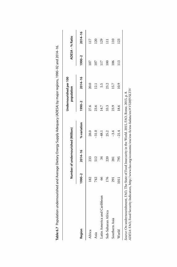
Tabl
e 6.
7 Po
pula
tion
unde
rnou
rishe
d an
d Av
erag
e D
ieta
ry E
nerg
y Su
pply
Ade
quac
y (A
DES
A) b
y m
ajor
regi
ons,
1990
–92
and
2014
–16.
Num
ber o
f und
erno
uris
hed
(Mill
ion)
Und
erno
uris
hed
per 1
00
popu
latio
nA
DES
A –
% R
atio
Regi
on19
90–2
2014
–16
% v
aria
tion
1990
–220
14–1
619
90–2
2014
–16
Afr
ica
182
233
28.0
27.6
20.0
107
117
Asi
a74
251
2−3
1.0
23.6
12.1
107
120
Latin
Am
eric
a an
d C
arib
bean
6634
−48.
114
.75.
511
712
9Su
b‐Sa
hara
n A
fric
a17
622
025
.233
.323
.210
011
1So
uthe
rn A
sia
291
281
−3.4
23.9
15.7
106
110
Wor
ld10
1179
5−2
1.4
18.6
10.9
113
123
Sour
ce: O
n un
dern
ouri
shm
ent,
FAO
, The
Sta
te o
f Foo
d In
secu
rity
in th
e W
orld
. 201
5, F
AO
, Rom
e, 2
015,
p. 8
.A
DES
A: F
AO
, Foo
d Se
curit
y In
dica
tors
, http
://w
ww.
fao.
org/
econ
omic
/ess
/ess
‐fs/
ess‐
fada
ta/e
n/#.
V52
0JV
SLT
IV
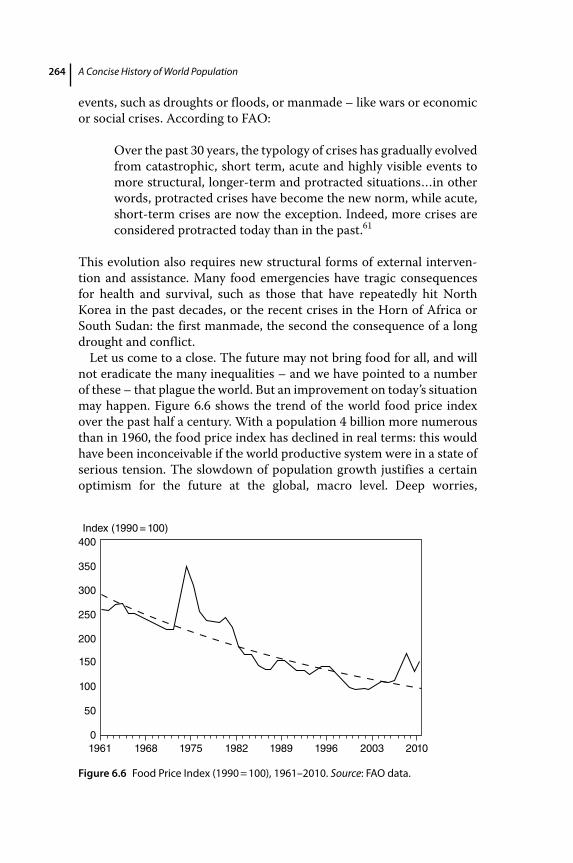
A Concise History of World Population264
events, such as droughts or floods, or manmade – like wars or economic or social crises. According to FAO:
Over the past 30 years, the typology of crises has gradually evolved from catastrophic, short term, acute and highly visible events to more structural, longer‐term and protracted situations…in other words, protracted crises have become the new norm, while acute, short‐term crises are now the exception. Indeed, more crises are considered protracted today than in the past.61
This evolution also requires new structural forms of external intervention and assistance. Many food emergencies have tragic consequences for health and survival, such as those that have repeatedly hit North Korea in the past decades, or the recent crises in the Horn of Africa or South Sudan: the first manmade, the second the consequence of a long drought and conflict.
Let us come to a close. The future may not bring food for all, and will not eradicate the many inequalities – and we have pointed to a number of these – that plague the world. But an improvement on today’s situation may happen. Figure 6.6 shows the trend of the world food price index over the past half a century. With a population 4 billion more numerous than in 1960, the food price index has declined in real terms: this would have been inconceivable if the world productive system were in a state of serious tension. The slowdown of population growth justifies a certain optimism for the future at the global, macro level. Deep worries,
19610
50
100
150
200
250
300
350
400Index (1990 = 100)
1968 1975 1982 1989 1996 2003 2010
Figure 6.6 Food Price Index (1990 = 100), 1961–2010. Source: FAO data.
The Future 265
however, come from the volatility of prices, the climate imponderable vagaries, the increasing number of protracted crises, the political c onflicts, the persistent deep geographic and social inequalities.
6.8 Space and Environment in a Smaller Planet
Let us come to the third question concerning the relation between population, space, and environment. Some aspects of this relation have already been touched upon in the preceding two sections: intensified human activity impacts nonrenewable resources and the demand for food, and therefore on land use and the environment. Increased demand for food, fibers, wood, and other natural resources leads to an extensification of agriculture and other human activities, generates land‐use modifications, intrudes on pristine areas, and exerts pressure on fragile environments. At the present time, population is 1,000 times or so more numerous than at the time of the invention of agriculture, 10,000 years ago, and devours an ever increasing amount of energy and natural resources. Ten thousand years ago, each human being had at his exclusive disposition a space endowment the dimensions of the Brazilian island of Fernando de Noronha, or of Robinson Crusoe’s island; today that exclusive space has been reduced to the dimensions of a football field. The face of Europe since the Middle Ages has changed profoundly as forest has receded in favor of cropland; a similar profound change has taken place in the Maghreb and in many areas of the Middle East. In the United States, the pristine woodland that covered much of the country east of the Mississippi, and from Canada to the Gulf of Mexico, had disappeared by the 1920s, swept away by population growth and industrialization. The mata atlantica (atlantic forest) covering the coastal region of Brazil had almost disappeared at the beginning of the nineteenth century, devoured by the extraction of valuable timber for the European market, demand for wood by the mining industry, and demand for fuel from the sugar cane plantations. In the Indian sub‐continent much of the forest cover was sacrificed to the demand for wood for shipbuilding, construction of the extensive railway system, and as fuel for running that system. At the global level, it has been estimated that between 1700 and 1990, over the total earth’s surface of 134.1 million km2, cropland has increased more than fivefold (from 2.7 to 14.7 percent) and pasture sixfold (from 5.2 to 31.0 percent), while the land covered by forest and woodland has receded from 54.4 to 41.5 percent; and grassland, steppe and tundra have declined from 32.1 to 17.5 percent.62 A more recent assessment (2007), based on high resolution satellite surveys, has determined that 54 percent of the entire surface of the earth is subject to a
A Concise History of World Population266
direct or indirect process of anthropization: this process includes cropland, pasture, managed forests, built‐up areas, urbanized areas, and land occupied by infrastructures for transportation, commercial and industrial activities.63 Less than half of the earth surface is, therefore, in a pristine (or semi‐pristine) state, much of it consisting of uninhabitable desert, arctic, or mountainous lands.
Anthropization and human intrusion in fragile environments are of foremost importance for the bionatural equilibrium of the world. The deforestation of the Amazon basin is, perhaps, the most worrying process, raising an intense debate. Estimates put the loss of forestland at between 15 and 20 percent, a phenomenon initiated in the 1940s for multiple factors: clearing land for crops and cattle under the pressure of the demand for food from a growing population; prospecting for oil and minerals and their exploitation; building infrastructures; settlement of immigrants. Other major pluvial forests – in the Congo basin, in Indonesia, in Papua New Guinea – are endangered by the pressure of human activity. Deforestation takes place in many other parts of the world and brings about profound modifications of the earth’s surface. According to FAO’s estimates,64 recent trends yield mixed results: at the global level the rate of deforestation has declined from 0.2 percent per year in 1990–2000 to 0.1 percent in 2000–10; however, deforestation goes on at high rates in Africa, Latin America, and the Caribbean, while forested land has increased in Europe and East Asia. At the aggregate country level, there is some evidence of a positive relationship between the rate of population growth and the rate of deforestation,65 but this relationship is relatively weak as there are other intermediate factors at work: opportunities for intensification, population density, and government regulations and institutions. Individual country studies, however, have clearly described situations in which deforestation has taken place under demographic pressure in contexts as different as the Philippines – where migration from the densely settled lowlands to the mountainous interior has led to rapid deforestation – Guatemala, Sudan, and Thailand.66 In general, there is a self‐reinforcing link between high population growth, poverty, and land degradation. Poverty is associated with high fertility since children – in the absence of health and pension systems – are an insurance against destitution. Scarcity of capital and basic resources – like water and fuelwood – sustains fertility, since c hildren provide needed labor and income. And high fertility determines high rates of population growth, which may further damage environmental resources, particularly when these are common property.67
The growth of built‐up areas for housing; for industrial, commercial, and recreational use; for communications; and for other purposes is another aspect of the transformation of land use that cannot go on
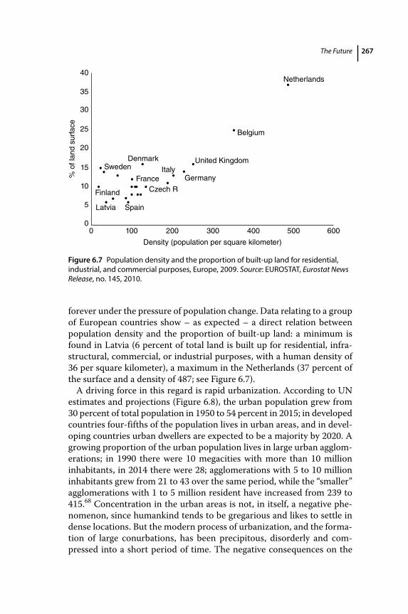
The Future 267
forever under the pressure of population change. Data relating to a group of European countries show – as expected – a direct relation between population density and the proportion of built‐up land: a minimum is found in Latvia (6 percent of total land is built up for residential, infrastructural, commercial, or industrial purposes, with a human density of 36 per square kilometer), a maximum in the Netherlands (37 percent of the surface and a density of 487; see Figure 6.7).
A driving force in this regard is rapid urbanization. According to UN estimates and projections (Figure 6.8), the urban population grew from 30 percent of total population in 1950 to 54 percent in 2015; in developed countries four‐fifths of the population lives in urban areas, and in developing countries urban dwellers are expected to be a majority by 2020. A growing proportion of the urban population lives in large urban agglomerations; in 1990 there were 10 megacities with more than 10 million inhabitants, in 2014 there were 28; agglomerations with 5 to 10 million inhabitants grew from 21 to 43 over the same period, while the “smaller” agglomerations with 1 to 5 million resident have increased from 239 to 415.68 Concentration in the urban areas is not, in itself, a negative phenomenon, since humankind tends to be gregarious and likes to settle in dense locations. But the modern process of urbanization, and the formation of large conurbations, has been precipitous, disorderly and compressed into a short period of time. The negative consequences on the
Netherlands
Belgium
United Kingdom
Germany
Denmark
ItalySweden
France
00 100 200 300 400 500 600
Density (population per square kilometer)
5
10
15
20
40
25
% o
f lan
d su
rfac
e
30
35
Czech R
SpainLatvia
Finland
Figure 6.7 Population density and the proportion of built‐up land for residential, industrial, and commercial purposes, Europe, 2009. Source: EUROSTAT, Eurostat News Release, no. 145, 2010.
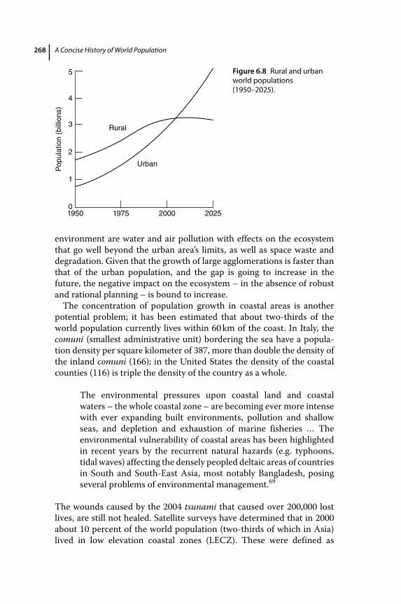
A Concise History of World Population268
environment are water and air pollution with effects on the ecosystem that go well beyond the urban area’s limits, as well as space waste and degradation. Given that the growth of large agglomerations is faster than that of the urban population, and the gap is going to increase in the future, the negative impact on the ecosystem – in the absence of robust and rational planning – is bound to increase.
The concentration of population growth in coastal areas is another potential problem; it has been estimated that about two‐thirds of the world population currently lives within 60 km of the coast. In Italy, the comuni (smallest administrative unit) bordering the sea have a population density per square kilometer of 387, more than double the density of the inland comuni (166); in the United States the density of the coastal counties (116) is triple the density of the country as a whole.
The environmental pressures upon coastal land and coastal waters – the whole coastal zone – are becoming ever more intense with ever expanding built environments, pollution and shallow seas, and depletion and exhaustion of marine fisheries … The environmental vulnerability of coastal areas has been highlighted in recent years by the recurrent natural hazards (e.g. typhoons, tidal waves) affecting the densely peopled deltaic areas of c ountries in South and South‐East Asia, most notably Bangladesh, posing several problems of environmental management.69
The wounds caused by the 2004 tsunami that caused over 200,000 lost lives, are still not healed. Satellite surveys have determined that in 2000 about 10 percent of the world population (two‐thirds of which in Asia) lived in low elevation coastal zones (LECZ). These were defined as
1950 1975 2000 2025
Urban
Rural
0
1
2
3
4
5
Pop
ulat
ion
(bill
ions
)
Figure 6.8 Rural and urban world populations (1950–2025).
The Future 269
contiguous areas along the coast less than 10 meters above sea level. These low‐lying areas are extremely fragile and also because of rising sea‐levels and their heavy urbanization. A more detailed analysis of China and Bangladesh – where one‐third of the world population of the LECZ lives – shows that the populations of these areas have grown between 1990 and 2000 at a rate double that of the rest of the respective country’s populations.70
Finally, a brief discussion of the interaction between population, atmospheric pollution, and climate change is in order, even if we cannot enter into complex technical details. A growing volume of human activity, and especially increased burning of fossil fuels, results in an increased concentration of “greenhouse gases” in the atmosphere; by blocking infrared radiation emitted from the earth’s surface, these gases may cause global warming with a variety of impacts on the environment and human activities. The emissions of greenhouse gases (three‐quarters carbon dioxide) between 1951 and 2010 have increased by an estimated 80 percent for the joint contribution of all human activities (production of energy, transportation, industrial, agricultural, commercial, and residential activities). The simulations conducted by the IPCC (Intergovernmental Panel on Climate Change), based on assumptions concerning population and economic growth and emission trends, confirm that global warming will continue throughout the century, and that in the period 2081 to 2100 the mean temperature of the planet will be higher (according to the various combinations of assumptions) by 1° to 4 °C than in the period 1986 to 2005.71 Adapting Ehrlich’s identity, we can say that the environmental impact of greenhouse gases is the result of the joint action of population, income, and technology changes. Bongaarts predicted, 20 years ago, that about half of the increase of greenhouse gases between 1985 and 2025 was the consequence of population growth.72
If population growth influences global warming, how, in return, will global warming affect demographic phenomena? A first consideration to be made is that, since the Paleolithic era, the human species has shown a remarkable adaptability to climate, settling at all latitudes and in the most extreme environments, unshielded by technology or by the experience accumulated over the millennia. Today, the population of about 1 million of the Siberian city of Irkutsk lives with an average yearly temperature of −1 °C (and the average temperature in January is −20 °C). The population of Muscat, capital of Oman, the same size as Irkutsk’s, at a latitude 29 degrees south of the Siberian city, lives with an average yearly temperature close to 30 °C. It is proposed that an increase of 2° or 3 °C over a century may not have relevant consequences, but this conclusion would be an oversimplification hiding several negative aspects of global warming. First, climate change would affect the different regions of the world
A Concise History of World Population270
in different ways, with more impact on marginal and fragile areas. More specifically, coastal areas would be much more vulnerable to flooding, with negative consequences for the population, particularly where densely settled. Second, large regions at low latitudes would become arid, with a loss of productivity for cereal and other crops. Third, there would be a geographic redistribution of pathogenic agents and, in the areas more affected by warming, an increasing incidence of infectious p athogens and of malnutrition, and finally, accrued risks for health and survival because of an increased frequency of heat waves, floods, and droughts.
The discussion in this and in the preceding sections reveals the complexity of the relationship between population growth and the environment. This relationship is affected in multiple ways by the number of inhabitants and by the volume and nature of human activities. The inevitable population growth of the first half of this century, together with an increasing degree of affluence, will determine an increased demand for commodities, food, and space; it will deplete some fixed resources and put increasing pressure on renewable ones. Technology may offset many undesirable effects, increasing substitution or abating pollution; and institutions may do the same, regulating land use, access to resources, and so on; while cultural changes may contribute through modified consumption patterns and changes in behavior. In the end, the negative effects of population growth – at least for the next century – may be neutralized and the limits to growth pushed forward. But three points have to be recognized: the first is that population growth is not neutral; the second is that a slowdown of growth will ease the solution of many problems; and the third is that never before have the human forces that threaten the living system of the planet been so strong. It is prudent to lessen the risks, and restraint of population growth will contribute to this end.73
6.9 Calculations and Values
Our discussion does not conclude on the side of either the optimists or the catastrophists. We can, however, attempt to understand whether the mechanisms of “choice” available to population, which allow for the regulation of growth as a function of perceived constraints, are weaker or stronger than they were in the past. Our closing reflections consider this question with regard to the perception of constraint and the functioning of mechanisms of choice and regulation.
Perception of the elements of constraint raises complex problems. Given the strength of population momentum, modifications of trends – for
The Future 271
example, a change in the supply of births – are only felt after a considerable delay. Moreover, certain “danger” signs are only slowly recognized: environmental deterioration, for example, is only fully p erceived after the damage has been done. The slow deforestation of a valley will lead to disastrous overflowing of the valley’s river, but only long after the process has begun. The “greenhouse effect,” created by the accumulation of carbon dioxide and other gases in the atmosphere, may only be felt after decades, and an initial warming phase may even be e rroneously interpreted as a positive development.
In traditional rural societies, awareness of the problems created by demographic growth was probably more immediate than it is in modern society. The inhabitants of a village, valley, or region experienced directly the negative effects of new settlement in an area already demographically saturated, and, while less efficient than those of the present day, regulating mechanisms of population change could gradually bring about the necessary adjustments. The expansion and integration of markets and the development of trade have contributed to masking, from individual perception, the link between natural resources (land, for example) and consumer goods. Hong Kong can grow beyond all measure, importing agricultural products from the United States or Argentina, without any awareness of the connection between the grain or beef consumed and the rural environment that produces them. China raises millions of pigs that are fed with soy imported from Brazil the growing of which impacts the Brazilian environment. Indonesia’s pluvial forests are cut down to make room for palm trees yielding oil whose demand is rapidly growing in other countries. This sort of detachment is a necessary consequence of economic development, but it should be pointed out that as a result the direct link between the protagonist of demographic choice (the individual) and the producer of the forces of constraint (the environment) has been broken. This link may be slowly reestablished if the individuals, institutions, and governments that now recognize the global nature and interconnectedness of environmental phenomena increase in number and prestige.
On a more immediate, economic level, price fluctuations should provide “danger” signs, announcing the imminent shortage of fundamental goods and therefore the need to correct the situation by lowering demand (which may in the long run have demographic implications) when it is no longer feasible to increase supply. The price system, however, does not always send out the right signals and a policy of subsidies may distort this process. Often cited are the adverse (demographic) effects, in poor countries, of those policies that keep basic food prices artificially low, compromising agricultural profits and further speeding migration to the already swollen cities. More generally, the noninclusion in prices of the
A Concise History of World Population272
negative externalities – such as the deterioration of the environment – determined by the economic activity constitutes a serious distortion of the “signal” that prices should be sending.
I have already discussed at length the mechanisms of choice and growth regulation (see Chapters 4 and 5), and clearly these have been enormously strengthened as a result of voluntary fertility control. Fertility regulation is spreading rapidly, although irregularly, making society more flexible in the face of the constraints it must face. While modern society may be better equipped with regard to the regulation of mortality and fertility than societies of the past, the same cannot be said with regard to another mechanism of choice, namely migration. The peopling of the world has been accomplished by means of migration and settlement that has distributed population according to existing or potential resources. Emigration has also always been the principal route of escape from poverty and destitution.74 This “freedom” of settlement, which in modern times has led to the Europeanization of temperate America and Australia, is today much impaired. In response to primarily political considerations, nations generally regard immigration as a marginal fact, acceptable only within a fairly rigid framework and in small numbers. Given the enormous national differences in income and assets and the relative ease of mobility, perhaps it could not have been otherwise. Nonetheless, it is also the case that there exists no open and available territory to act as an outlet for demographic excess and to colonize with human population, plants, and animals.75 In addition, greater economic integration is accompanied by greater separation of peoples and ethnic groups; the creation of new national states, often bounded by unnatural borders, has led to the redistribution of ethnic groups, previously mixed, within well‐defined political units; and a tendency toward segregation between groups is also frequent within national borders. So the effectiveness of an important tool of “choice,” migration, has declined as compared to the past.
Our balance sheet, then, has both credit and debit entries, and it is not easy to calculate the bottom line, though the ability to control fertility, when it becomes universal, will constitute the decisive factor for c ontrolling growth.
More and more one hears that the control of population growth has been accepted as a positive value and so does not require demonstration or confirmation. All things considered, this is a fortunate development for demographers, who will no longer be obliged to demonstrate the advantages of this or that trend. Our environment is certainly finite, even if its limits can be repeatedly expanded, and unlimited growth cannot continue without increasing risks. This observation should be sufficient to support the conviction that the human race must prepare itself for a long phase of demographic moderation, and in some cases reversal.
The Future 273
Another factor should be kept in mind: beyond certain limits, demographic growth creates diseconomies of scale, reversing a trend that seems to have dominated much of human history. Consider the unrestrained growth of urban agglomerations in poor countries (see Section 8, this chapter): social, sanitary, and environmental problems associated with this growth will involve management difficulties that increase at a greater rate than the aggregate they concern. Other diseconomies of scale will be encountered in the areas of poverty, malnutrition, and illiteracy: even in the context of general economic progress, rapid demographic growth brings with it – in spite of a decrease in the overall frequency of these social blights (expressed as a percentage of total population) – an increase in the absolute numbers of the poor, malnourished, and illiterate. Programs designed to address the problems of a smaller population may well run into greater than proportional problems. The situation for malnutrition and education is analogous, given a large increase in the number of the hungry and the illiterate. Or, again, natural catastrophes like floods and droughts, or the tsunami that devastated the Indonesian, Indian, and Thai coasts at the end of 2004 and Japan in 2011 – or human‐made ones, striking more densely populated areas or regions, demand relief programs that, forced to cope with large populations, are hard to manage and organize. In many cases the elimination of a problem becomes proportionately more difficult as its dimensions grow; this is a diseconomy of scale.
It is therefore likely that we are entering an historical phase – of indeterminate length – during which population growth will cease to produce economies of scale and may well start producing overwhelming diseconomies. So justifications for the control of population growth do exist; and as that control is becoming an accepted element in the strategy of global survival it tends to be less and less a matter of calculations and more and more one of values.
It is a common perception that current population growth is like a vehicle speeding along a dangerous road. The road represents resources that are believed to be limited (they are, but they are also very elastic). At the end of the road there is a ravine. Our vehicle covers the road at a fantastic speed, approaching the ravine and disaster. There are two teams working on the problem. One tries to improve the road, either bypassing the ravine or building a bridge over it – that is human ingenuity trying to economize needed resources, substitute one with another, or invent new ones. The other team works on the vehicle, but there are disagreements. Some want to reduce power and speed so that more time will elapse before the ravine is approached. Others want to improve the steering, brakes, and suspension, so that the driver is able to drive safely, adjusting to the characteristics of the road, accelerating, slowing down, or coming
A Concise History of World Population274
to a stop if needed. This is the best vehicle, able to maneuver and to choose the safer course, with a responsible driver able to see the signs of danger.
Notes
1 Examples can be found even in the twentieth century. Consider the disastrous effects of forced collectivization during the Chinese Great Leap Forward of 1958–62 (30 million more deaths than normal in 4 years) or the similar effects of the 1932–3 crisis in the Soviet Union, certainly worsened by collectivization carried out in the countryside. See B. Ashton, K. Hill, A. Piazza, and R. Zeitz, “Famine in China 1956–81,” Population and Development Review 10 (1984); A. Blum, “Redécouverte de l’Histoire de l’URSS (1930–1945) [Rediscovering the History of the USSR (1930–1945)],” Population et Société 253 (January 1991); A. Graziosi, ed., Lettere da Kharkov [Letters from Kharkov] (Einaudi, Turin, 1991); M. Livi‐Bacci, “On the Human Costs of Collectivization in the USSR,” Population and Development Review 19:4 (1993); S. Adamets, “Famine in 19th and 20th Century Russia: Mortality by Cause, Age and Gender,” in C. Ó Gráda and T. Dyson, eds., Famine Demography Perspectives from Past and Present (Oxford University Press, Oxford, 2002); F. Dikötter, Mao’s Great Famine: The History of China’s Most Devastating Catastrophe, 1958–62 (Walker, New York, 2010).
2 National Research Council, Beyond Six Billion: Forecasting the World Population (National Academy Press, Washington, DC, 2000).
3 United Nations, World Population Prospects. The 2015 Revision (New York, 2015).
4 A set of probabilistic projections to 2100 have been made by W. Lutz, W. C. Sanderson, and S. Scherbov, eds., The End of World Population Growth in the 21st Century: New Challenges for Human Capital Formation and Sustainable Development (Earthscan, London and Sterling, VA, 2004). The authors have calculated a series of 2,000 projections for 13 world areas based on a set of possible combinations of fertility and survival functions. As far as the world population is concerned, in 60 percent of the cases it will remain below 10 billion in 2100; in 86 percent of the cases, it will reach a maximum before 2100. Less interesting is the attempt to explore the p ossible future course of the world population up to the year 2300, given the unpredictability of the long‐term trends of fertility and mortality. See United Nations, World Population in 2300 (New York, 2003).
5 G. McNicoll, “Population Weights in the International Order,” Working Paper, no. 120 (Population Council, New York, 1999); J. Goldstone, “The New Population Bomb,” Foreign Affairs 89:1 (2010). P. Demeny,
The Future 275
“Geopolitical Aspects of Population in the Twenty‐First Century,” Population and Development Review, 3:4 (2012).
6 J. Bongaarts and R. Bulatao, “Completing the Demographic Transition,” Working Paper, no. 125 (Population Council, New York, 1999).
7 D. J. Hatton and J. G. Williamson, The Age of Mass Migration: Causes and Economic Impact (Oxford University Press, Oxford, 1998).
8 United Nations, World Population Prospects. The 2010 Revision. For an extended survey of international migration, United Nations, World Economic and Social Survey 2004. International Migration (New York, 2004).
9 M. Livi‐Bacci, “Riflessioni su Integrazione, Disuguaglianze e Migrazioni Internazionali [Reflections on Integration, Inequality and International Migration],” in A. Quadrio Curzio, ed., La Globalizzazione e i Rapporti Nord–Est–Sud [Globalization and North–East–South Relations] (Il Mulino, Bologna, 2004); M. Livi‐Bacci, A Short History of Migration (Polity, Cambridge, 2012).
10 Livi‐Bacci, A Short History, OECD, International Migration Outlook, SOPEMI 2010 (Paris, 2010).
11 Global Commission on International Migration, Migration in an Interconnected World: New Directions for Action – Report of the Global Commission on International Migration (Geneva, 2005), p. 77.
12 J. Bhagwati, “Borders Beyond Control,” Foreign Affairs 82:1 (2003).13 G. Tapinos and G. Delaunay, “Can One Really Talk of Globalization of
Migration Flows?,” in OECD, Globalization, Migration and Development (Paris, 2000). 13th International Panel on Climate Change (IPCC), Climate Change 2014. Impact, Adaptation and Vulnerability, p. 767 (www.IPCC‐wg2.gov/AR5/), accessed March 1, 2016. For a rather pessimistic view on the subject, see the report of the US National Intelligence Council and the excerpts selected in “Effects of Future Climate Change on Cross‐Border Migration in North Africa and India,” Population and Development Review, 36:2 (2010).
14 National Research Council, Beyond Six Billion.15 On the complex topic of human longevity: K. W. Wachter and
C. E. Finch, eds., Between Zeus and the Salmon. The Biodemography of Human Longevity (National Academy Press, Washington, DC, 1997); B. Carnes and S. J. Olshansky, “A Realistic View of Aging, Mortality and Future Longevity,” Population and Development Review 33:2 (2007).
16 J. Lederberg, R. E. Shope, and S. C. Oaks, eds., Emerging Infections (National Academy Press, Washington, DC, 1992), p. 84.
17 Lederberg et al., Emerging Infections; WHO, World Health Report 1998. Life in the 21st Century (Geneva, 1999); G. Rezza, Epidemie. Origini ed Evoluzione [Epidemics: Origins and Evolutions] (Carocci, Rome, 2010), pp. 61–82. In 2014–15, the Ebola epidemic in West Africa caused 11,301
A Concise History of World Population276
deaths out of 28,603 cases, http://apps.who.int/ebola/sites/default/files/atoms/files//who_ebola_situation_report_03‐02‐2016.pdf, accessed February 15, 2016.
18 UNAIDS, Trends in HIV Incidence and Prevalence (Geneva, 1999); Rezza, Epidemie, pp. 83–90.
19 R. C. H. Shell, “Halfway to the Holocaust: The Rapidity of the HIV/AIDS Pandemic in South Africa and its Social, Economic and Demographic Consequences,” Proceedings of the Third African Population Conference, vol. 1 (Durban, 1999).
20 T. Dyson, “HIV/AIDS and Urbanization,” Population and Development Review 29:3 (2003).
21 UNAIDS, Aids Epidemic Update. December 1999 (Geneva, 1999); UNAIDS, Report on the Global HIV/AIDS Epidemic (Geneva, 1998).
22 Shell, Halfway to the Holocaust, pp. 164–5.23 Shell, Halfway to the Holocaust, p. 151.24 United Nations, World Population Prospects. The 2015 Revision
(New York, 2015).25 M. V. Shkolnikov and G. A. Cornia, “Population Crisis and Rising Mortality
in Transitional Russia,” in G. A. Cornia and R. Paniccià, eds., The Mortality Crises in Transitional Economies (Oxford University Press, Oxford, 2000); G. A. Cornia and R. Paniccià, “The Transition’s Population Crisis: Nuptiality, Fertility, and Mortality Changes in Severely Distressed Economies,” in M. Livi‐Bacci and G. De Santis, eds., Population and Poverty in Developing Countries (Oxford University Press, Oxford, 2000); A. Andreev, “Réaction d’une Population Hétérogène à une Perturbation. Un Modèle d’Interprétation des Evolutions de Mortalité en Russie [Reaction of a Heterogeneous Population to Shocks. A Paradigm for the Interpretation of Mortality Change in Russia],” Population 1 (January–February 1997).
26 Cornia and Paniccià, Mortality Crises; United Nations, World Population Monitoring 1998. Health and Mortality. Selected Aspects (UN, New York, 2000), pp. 16–17.
27 N. G. Bennett and S. J. Olshansky, “Forecasting US Age Structure and the Future of Social Security,” Population and Development Review 22:4 (1996), p. 708. J. Bongaarts, “Trends in Causes of Death in Low‐mortality Countries: Implications for Mortality Projections,” Population and Development Review, 40:2 (2014).
28 An increase of health expenditure (in percent of GDP) may determine a shift of the expenditure from the public to the private sector, increasing inequality in the access to health facilities and care. This may have a n egative consequence on survival.
29 OECD, Health at a Glance 2015, Paris, 2015, p. 216.30 J. Dupâquier, ed., L’Espérance de Vie sans Incapacité [Life Expectancy
without Disability] (PUF, Paris, 1997); V. Egidi, “Health Status of Older People,” Genus 59:1 (2003).
The Future 277
31 Many authors believe that life expectancy will continue to increase in the future, reaching 100 years towards the end of this century: an optimism that this author does not share.
32 An exhaustive review of the definitions and concepts implicit in the expression “carrying capacity” can be found in J. E. Cohen, How Many People Can the Earth Support? (Norton, New York, 1995), pp. 419–25. Indeed the whole book is dedicated to an analysis and dissection of this concept.
33 G. Ortes, “Riflessioni sulla Popolazione delle Nazioni per Rapporto all’Economia Nazionale [Reflections on the Population of Nations in Relation to the National Economy]” (1790), in Scrittori Classici Italiani di Economia Politica [Classic Writings of Italian Political Economists] (G. G. Destefanis, Milan, 1804), vol. 24, p. 28.
34 D. H. Meadows, D. L. Meadows, and J. Randers, Beyond the Limits: Global Collapse or a Sustainable Future? (Earthscan, London, 1992). For a survey of the debate, V. Smil, “Limits to Growth Revisited: A Review Essay,” Population and Development Review 31:1 (2005).
35 Cohen, How Many People, pp. 216–21.36 Cohen, How Many People, pp. 402–25.37 C. T. De Wit, “Photosynthesis: Its Relation to Overpopulation,” in A. San
Pietro, F. A. Greer, and T. J. Army, eds., Harvesting the Sun: Photosynthesis in Plant Life (Academic Press, New York, 1967), pp. 315–20.
38 C. Clark, Population Growth and Land Use (Macmillan, London, 1977).39 R. Revelle, “The Resources Available for Agriculture,” Scientific
American (September 1976), pp. 164–79.40 B. Gilland, “Considerations on World Population and Food Supply,”
Population and Development Review 9:2 (1983). A more recent view by the same author is “World Population and Food Supply. Can Food Production Keep Pace with Population Growth in the Next Half Century?” Food Policy 27 (2002), pp. 47–63. B. Gilland, Population and Overpopulation (Copenhagen, 2011).
41 FAO = Food and Agricultural Organization (of the UN); IIASA = International Institute for Applied Systems Analysis. Cohen, How Many People, pp. 196–209.
42 V. Smil, “How Many People can the Earth Feed?” Population and Development Review 20:2 (1994); FAO, World Agriculture Towards 2015–2030 (Rome, 2002).
43 Edward O. Wilson, The Future of Life (New York, Knopf, 2002).44 World Resources Institute, World Resources, pp. 8–11.45 UNEP, Decoupling Natural Resources and Environmental Impacts from
Economic Growth (UNEP, 2011). Table 2.146 World Resources Institute, World Resources, p. 6.47 World Bank, http://databank.worldbank.org/data/download/GNIPC.
pdf, accessed February 17, 2016.
A Concise History of World Population278
48 P. Demeny, “Population and Development,” in IUSSP, Distinguished Lecture Series on Population and Development, International Conference on Population and Development, Cairo, 1994.
49 I. Stern, “The Environmental Kuznets Curve,” International Encyclopaedia of Ecological Economics (June 2003). This curve models the emission p attern, which is a function of material inputs.
50 P. R. Ehrlich and J. P. Holdren, “Impact of Population Growth,” Science 171 (1971), pp. 1,212–17.
51 The (proved) reserve to production ratio, or reserve‐life index, is an extremely raw indicator. For copper, it has oscillated around 40 years, from 1950 to the present (http://copperalliance.org/wordpress/wp‐content/ uploads/2013/06/ica‐long‐term‐availability‐1303‐A4‐lr.pdf). For oil and for gas it has increased, between 1980 and 2012, from 28 to 47, and from 49 to 59 years, respectively (https://books.google.it/books?id=LekD AAAAQBAJ&pg=PA102&dq=iron+ore+reserve+to+production+ratio& hl=it&sa=X&ved=_wQ6AEIPTAD#v=onepage&q=iron%20ore%20 reserve%20to%20production%20ratio&f=false. According to the World Bank, between 2001 and 2010–11, out of nine minerals considered, the ratio has increased for nickel, copper, and silver; has remained approximately stable for gold, lead, and zinc, has declined for tin, iron ore, and bauxite (aluminum). See World Bank, Global Economic Prospects, vol. 7, June 2013, p. 102. A very interesting recounting of the debate between environmentalists and their critics, can be found in P. Sabin, The Bet: Paul Ehrlich, Julian Simon, and our Gamble over the Earth’s Future, (New Haven, Yale University Press, 2013).
52 FAO, The State of Food Insecurity in the World. 2015, FAO, Rome, 2015, p. 8. N. Alexandratos, “Governments, Markets, and the Ending of Hunger: A Review Essay,” Population and Development Review, 41: 4 (2015).
53 Piero Conforti, ed., Looking Ahead in World and Food and Agriculture. Perspectives to 2050, Rome, FAO, 2015; B. Gardner, Global Food Futures: Feeding the World in 2050 (London, Bloomsbury, 2013).
54 The World Bank, World Development Report 1992: Population and Environment (Oxford University Press, Oxford, 1992), p. 134.
55 World Bank, World Development Report 1992.56 I. Serageldin and G. J. Persley, Promethean Science: Agricultural Biotechnology,
the Environment and the Poor (CGIAR, Washington, DC, 2000).57 FAO, Food Security Indicators, http://www.fao.org/economic/ess/ess‐fs/
ess‐fadata/en/#.V520JVSLTIV58 Hunger, currently used, is a rather vague concept, and is often substituted
by the term “undernourished.” “The measure for hunger compiled by FAO, defined as undernourishment, refers to the proportion of the population whose dietary energy consumption is less than a pre‐determined threshold. This threshold is country specific and is measured
The Future 279
in terms of the number of kilocalories required to conduct sedentary or light a ctivities. The undernourished are also referred to as suffering from food deprivation.” (http://www.fao.org/docrep/013/al936e/al936e00.pdf)
59 The indicator expresses the Dietary Energy Supply (DES, National average energy supply, expressed in calories per capita per day) as a percentage of the Average Dietary Energy Requirement (ADER, which expresses the adequate nutrition in the population). Each country’s or region’s average supply of calories for food consumption is normalized by the average dietary energy requirement estimated for its population to provide an index of adequacy of the food supply in terms of calories.
60 Given the unequal distribution of food in a population, an ADESA index below 115–120 signals the existence of serious hunger‐related problems.
61 FAO, The State of Food Insecurity, cit., p. 38.62 Klein Goldenwijk and Navin Ramankutty, “Land use Changes during the
Past 300 years,” in Encyclopedia of Life Support Systems (EOLSS), vol. 1(UNESCO, Paris, 2005).
63 Roger Leb Hooke, José F. Martín‐Duque, Javier Pedraza, “Land Transformation by Humans: A Review,” GSA Today, December 2012.
64 FAO, State of the World’s Forests (FAO, Rome, 2011).65 S. H. Preston, “Population and Environment from Rio to Cairo,” in
IUSSP, Distinguished Lecture Series on Population and Development (International Conference on Population and Development, Cairo, 1994), p. 8; R. E. Bilsborrow, “Population, Development and Deforestation: Some Recent Evidence,” in Population, Environment and Development (UN, New York, 1994).
66 Bilsborrow, Population, Development and Deforestation, pp. 129–31.67 N. Cuffaro, “Population Growth and Agriculture in Poor Countries: A
Review of Theoretical Issues and Empirical Evidence,” World Development 25:7 (1997), p. 1,158; P. Dasgupta, An Inquiry into Well‐Being and Destitution (Clarendon Press, Oxford, 1993).
68 United Nations, World Urbanization Prospects. The 2014 Revision (UN, New York, 2014).
69 B. Zaba and J. I. Clarke, “Introduction: Current Directions in Population–Environment Research,” in B. Zaba and J. I. Clarke, eds., Environment and Population Change (Ordina, Liège, n.d. [1994]), p. 24.
70 Gordon McGranahan, Deborah Balk, and Bridget Anderson, “The rising tide: assessing the risks of climate change and human settlements in low elevation coastal zones,” Environment & Urbanization, 19:1 (2007); World Bank, Climate Risks and Adaptation in Asian Coastal Megacities, Washington, 2010.
71 International Panel on Climate Change, IPCC, Climate Change 2014, Synthesis Report. Summary for Policymakers, https://www.ipcc.ch/pdf/assessment‐report/ar5/syr/AR5_SYR_FINAL_SPM.pdf accessed February 24, 2016.

A Concise History of World Population280
72 J. Bongaarts, “Population Growth and Global Warming,” Working Paper, no. 37 (Population Council, New York, 1992).
73 See the relatively optimistic view of National Research Council, Our Common Journey: A Transition towards Sustainability (National Academy Press, Washington, DC, 1999), p. 160; “A successful transition towards sustainability is possible over the next two generations. This transition could be achieved without miraculous technologies or drastic transformations of human societies.”
74 J. K. Galbraith, The Nature of Mass Poverty (Penguin, Harmondsworth, 1980).
75 A. W. Crosby, Ecological Imperialism. The Biological Expansion of Europe, 900–1900 (Cambridge University Press, London, 1986).
281
A Concise History of World Population, Sixth Edition. Massimo Livi-Bacci. © 2017 John Wiley & Sons Ltd. Published 2017 by John Wiley & Sons Ltd.
Major Scientific Journals for Further Reading
Ageing & Society
Demographic Research
Demography
European Journal of Population
Genus
International Migration
International Migration Review
Journal of Population Economics
Journal of Population Research
N-IUSSP – IUSSP’s Online News Magazine
Population
Population and Development Review
Population studies
283
A Concise History of World Population, Sixth Edition. Massimo Livi-Bacci. © 2017 John Wiley & Sons Ltd. Published 2017 by John Wiley & Sons Ltd.
Index
Page references to Figures or Tables will be in italics, followed by the letters ‘f ’ or ‘t ’ as appropriate, while references to Notes will be followed by the letter ‘n’ and Note number.
Aboriginal populations, 20, 21f, 39, 51, 99
abortion, 183, 185, 191, 196, 199, 202and infanticide, 35, 66selective, 195, 198
abscissa, 17adaptation process, 34–35, 62, 76n28adoption, 68Africa
birth control, 182birth intervals, 55Central Africa, 244Eastern Africa, 214n15#fertility, 181migration, 102, 246North Africa, 40, 217n40, 261political sustainability, 248populations, 67, 213n2and slave trade, 48, 53–57South Africa, 40, 210, 221n85, 244sub‐Saharan Africa, 19, 32n34, 173,
179, 181, 206, 208f, 214n15, 217n40, 246, 258, 262
survival conditions, 172age, maternal, 11, 12agricultural transition, 35
and nutrition, 37, 38, 40, 75n20, 99presumed demographic effects,
40, 41f
see also agriculture; demographic transition; Neolithic Age
agriculture, ix, 42and demand for food, 259and demographic growth, 115n29effect of demographic growth on
economic development of agricultural societies, 85
employment in, 140forest‐fallow cultivation, 96, 101and hunter‐gatherers, 98–99indices of cultivation and labor
intensity, 101, 115n31innovations, 95, 96, 97, 100intensification process, 96, 97f, 101invention of shares, 100land cultivation systems, 96slash‐and‐burn systems, 96, 97, 101tools, 86, 96, 101see also agricultural transition;
farming/farmers; hunter‐gatherer populations
AIDS epidemic see HIV/AIDsAmerica
Africa and slave trade, 53–57external expansion, 107Indios, American, 47–53see also United States
Ammerman, A. J., 74n3, 74n6, 103
Index284
Andreoni, Giovanni Antonio, 56Angiola, Caterina (later Battista), 7, 8animals
domestication, 37, 39, 73n3and humans, 1–5lower vulnerability of larger animals,
3–4pathogens affecting, 39r and K vital strategies, 1, 3f, 16, 28n3rapid growth and decline, 5
Annan, Kofi, 240anovulatory period, 10antiretroviral drugs (ART), 244Armelagos, G. J., 38Arnhem Land Aborigines, 99Asia, 182, 183, 268
Eastern Asia, 19, 102, 172, 179, 266, 268
economic inequalities, 238labor force, 206, 208fpopulation doubling, 67South East Asia, 181, 195, 198, 241Southern Central Asia, 172, 181, 262
asylum rights, 239Australia
Aboriginal population, 20, 21f, 39, 51, 99
mouse, 5Average Dietary Energy Supply Adequacy
(ADESA), 262, 263tAzara, Félix de, 80–81n83Aztec Empire, Spanish conquest, 48, 49,
51, 52
Bates, Réal, 28n9Battista, Giovan, 7, 8Bichi, Andrea (laster Fossi), 7Bichi, Filippo, 7Bichi, Jacopo, 7–8Bichi, Maria Maddalena, 7Binswagen, H. R., 101biological sustainability, 243–244biomass production, 20biotechnology applications, 261Biraben, J. N., 26, 36, 74n4, 76n31birth control, 69, 141, 159n14
demographic growth, 11, 17–18, 19
fertility levels, 131–132, 133in poor countries, 181, 182, 184, 185,
186, 193, 195–196, 199, 202, 203, 214n16, 216n32
traditional and modern methods, 182, 216n32
“unmet need” for, 187, 216n37see also family planning
birth intervals, 12, 40, 55, 68, 131, 181longer, 196shorter, 183, 214n15
birthsassumptions relating to, 28n11frequency of, 10–11infertility period following, 10life expectancy at birth, 9, 13, 15, 27,
71, 191Black Death (1348), 45, 91
see also plaguebody, physical characteristics
body length and interval between successive generations, 3, 4f
body weight and age of sexual maturity, 28n5
Boleda, Mario, 28n9Bongaarts, J., 12, 28n11, 28n12,
161n20, 269Borah, W., 50, 76n49Boserup, E., 97–98, 100, 102Bourgeois‐Pichat, J., 26Brazil, 78n50, 181, 206, 244, 265, 271
slave trade, 55, 56, 58breast‐feeding, duration, 10, 12, 133Bronze Age, 1brush‐fallow cultivation, 96buckwheat, 72built‐up areas, growth of, 266–267Bushmen of Kalahari, 99
Cairo United Nations Conference on Population and Development (1994), 187
Canadafertility rates, 59–60French migration to, 60, 61tland cultivation, 140population size and prosperity, 110
Index 285
St Lawrence basin/valley, 8, 57, 58see also French Canadians; North
America; QuébecCaribbean islands, slave trade, 54–55, 56carrying capacity (CP), 251, 253, 277n32Cartier, Jacques, 58Caselli, G., 127–128Catherine the Great, 106Cavalli Sforza, L. L., 74n3, 103censuses, population, 24, 55, 57, 62, 194central Mexico, 50, 53Champlain, Samuel de, 8Charbonneau, H., 28n9, 50–51, 80n82Chayanov, V., 211child rearing costs, 185–186Chile, 178, 184, 213n2China
age structures, 199, 200fcity growth, 111Community Party, Central
Committee, 199Cultural Revolution, 196demographic diversity, 168demographic growth, 68demographic indices, 192tdynasties, 24Eighth Party Congress (1956), 195and Europe, 67–68family planning programs, 195family system, 68Fifth National People’s Assembly
(1979), 196future projections, 269Great Leap Forward, 196, 197and India, 191, 192t, 193–199,
200f, 201infanticide of baby girls, 67–68, 69one‐child policy, 197, 198pre‐1980s population policy, 218n57sixth census of PRC, 24survival conditions, 172Taiping War (1851–1864), 68and TFR, 197, 198
choice, 34, 270Cipolla, Carlo, 19, 22, 45city growth, 110–111Clark, Colin, 115n20, 117n57, 253
climate change, 34, 241–242Club of Rome, 89, 147, 258–259Coale, Ansley, 160n17, 194, 220n73Cobbett, William, 72Cohen, Joel, 253Cohen, Mark N., 74n7, 75n20, 98, 99colonists, 58, 97
and demographic decline of indigenous populations, 47, 48, 50, 51, 52
German, 106, 107Columbus, Bartolomé, 48Columbus, Christopher, 47Connell, K. H., 62, 63, 64, 81n91conquistadors, 51constraint, forces of, 19–24, 34, 35,
226, 270contraception see birth controlCook, F., 50, 76n49Corsini, Carlo, 28n8Cortés, H., 1Costa Rica, 178Crosby, A. W., 80n83Cuba, 49, 78n48, 178cycles of growth and decline, 2, 9, 19, 27,
33, 42Malthusian model, 91
Darwin, Charles, 4, 51DDT spraying, 176, 201De Wit, T., 253death see mortalityDeevey, E. S., 23, 24deforestation, 266Del Buono, Domenica, 7–8Democratic Republic of Congo
(DRC), projected increase in population, 5
demographic aging, 145, 162n32demographic and economic growth
relationshipagricultural societies, 85empirical observations, 150, 151t,
152–157Fertilia and Sterilia, 202opposing views, 85in poor countries, 211–212
Index286
technical progress, 85theoretical considerations, 146–150
purely demographic factors, 148scale and dimensional factors,
148–149stock of knowledge and
technological progress, 149–150see also demographic pressure, and
economic development; diminishing returns
demographic change, 34, 62, 104in poor countries, 168see also demographic decline;
demographic growthdemographic decline
aggregate, 36alternating with growth cycles, 2, 9,
19, 27, 33, 91disappearance of populations, 5, 34,
35, 51lack of immunity in native
populations, 48in New World, 48periodic elimination of excess
population in crisis years, 89plague in Europe, 42–47and standard of living, 95see also demographic growth
demographic growth, 33–84adaptation process, 34–35Africa, America and slave trade,
53–57aggregate, 36and agriculture, 115n29alternating with stagnation, 1–2, 9, 33,
42, 91China, 68choice, 34constraint, forces of, 19–24, 34,
35, 226current growth, 273–274cycles of growth and decline, 2, 9, 19,
27, 33, 42, 91data, 25–26
and diminishing returns, 85–89and domestication of plants and
animals, 73n3economies of scale resulting from,
149–150energy, 22, 23, 32n34equilibrium, maintaining, 5, 87families see familiesfast, as harmful to economic growth,
209–210French Canadians, 57–61growth potential of a population
incompatible with resources necessary for survival (Malthus), 86–87
measures, 9–10humans and animals, 1–5Indios, American, 47–53Ireland, 62–63, 67Japan, 65–67limits of, 23–24and migration, 102–103, 234tand mortality decline, 122–123Neolithic demographic transition,
35–42obstacles to, 19r and K vital strategies, 2, 3f, 16, 28n3rapid, 5–6, 7t, 113, 258reasons for following particular
path, 2relationship with economic growth
see demographic and economic growth relationship
space of growth, 17–19, 33statistics, 24–27as threat to health and social order,
225–226variations in rates, 6and wealth, 95see also demographic decline
demographic order, 62, 145, 225demographic pressure, 137
and economic development, 94–101examples from Stone Age to
present day, 98–101and migration, 142–143
demographic and economic growth relationship (cont’d)
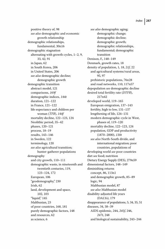
Index 287
positive theory of, 98see also demographic and economic
growth relationshipdemographic relationships,
fundamental, 30n16demographic stagnation
alternating with growth cycles, 1–2, 9, 33, 42, 91
in Japan, 62in South Korea, 206in United States, 206see also demographic decline;
demographic growthdemographic transition
abstract model, 121comparisons, 169fdemographic indices, 144tduration, 121–122in France, 121–122life expectancy and children per
woman (TFR), 144fmortality decline, 122–123, 124Neolithic period, 35–42phases, 120–121process, 18–19results, 143–146in Sweden, 122terminology, 120see also agricultural transition;
hunter‐gatherer populationsdemography
and city growth, 110–111demographic waste, in nineteenth and
twentieth centuries, 119, 123–124, 172
European, 106“geodemography,” 230Irish, 62land, development and space,
102, 103“liquid,” 145Malthusian, 23of poor countries, 168, 181purely demographic factors, 148and resources, 62as science, 6
see also demographic aging; demographic change; demographic decline; demographic growth; demographic relationships, fundamental; demographic transition
Denison, F., 148–149Denmark, growth rates, 18density of population, 1, 18, 21f, 22
and agricultural systems/rural areas, 95, 97
prehistoric populations, 76n28and road networks, 110, 117n57
depopulation see demographic declinedesired total fertility rate (DTFR),
217n42developed world, 119–165
European emigration, 137–143fertility, high to low, 131–137lengthening of life, 124–131modern demographic cycle in West,
phases of, 119–120mortality decline, 122–123, 124population, GDP and productivity
(1870–2000), 130tsee also North‐South divide, and
international migration; poor countries, populations of
developing world see poor countriesdiet see food; nutritionDietary Energy Supply (DES), 279n59dimensional factors, 148–149diminishing returns
concept, 86, 113n1and demographic growth, 85–89logic, 94Malthusian model, 87see also Malthusian model
disability‐adjusted life years (DALYs), 179
disappearance of populations, 5, 34, 35, 51diseases, 34, 38–39
AIDS epidemic, 244, 245f, 246, 247t, 248
and biological sustainability, 243–244
Index288
burden of disease, estimates, 179, 180tcholera, 69, 126, 244diseases of white European colonists,
native populations succumbing to, 48–49, 51, 52
frequency and transmission of infectious diseases, 41–42
malaria, 39, 53, 173, 176, 178, 201, 243plague, and demographic decline in
Europe, 42–47smallpox, 47–48, 52syphilis, 243, 244tuberculosis, 178, 243, 244see also epidemics; infections;
mortalitydivide and multiply strategy, 5–6, 7tdivision of labor, 109Drang nach Osten (drive to the east), 106
ecological niches, 39economic development, and
demographic pressure see demographic pressure, and economic development
economic inequalities, 238–239economic sustainability, 249–251economies of scale, 109, 110, 211
and demographic growth, 149–150diseconomies of scale, 273
ecosystem, 98, 268complexity, 39demographic growth, 25, 36, 37, 39
Ehrlich, P. R., 257, 258encomienda system (allotment of natives
to colonists as indentured labor), 48, 49
energyAverage Dietary Energy Requirement
(ADER), 279n59Average Dietary Energy Supply
Adequacy (ADESA), 262, 263tdemographic growth, 22, 23, 32n34Dietary Energy Supply (DES), 279n59requirements in United States, 147
Englandaverage height of citizens, 73
British imperialism, 137demographic growth, 5, 6, 69–70
and economic growth, 150as demographically small country, 150emigration from, 58, 107France compared, 69, 94, 137industrialization, 140investment abroad, 138Ireland compared, 62–63life expectancy, 71, 127, 128and Malthusian model, 92–93plague in, 42, 45potato consumption, 72war with France, 64see also Great Britain; Industrial
Revolutionenvironment
and climate change, 34, 241–242constraint, forces of, 19–24, 34, 35,
226, 270and space, in smaller planet, 265–270
environmental friction, 19epidemics, 39, 44, 49, 53, 65, 76n28, 92,
97, 126AIDS, 244, 245f, 246, 247t, 248smallpox (1518–1519), 47–48, 52see also diseases; infections
equilibriumbionatural, 266demographic/population, 124, 226maintaining, 5, 124, 153new, 87precarious, 62re‐establishing, 35, 87, 88, 123sigmoid approach to, 252fvirtual, 6
Europe, 67, 69, 71–73agricultural system, ixcontinent, extension of, 103demographic acceleration in
eighteenth century, 69and developed world see developed
worldemigration, European, 137–143growth of selected populations
(1600–1850), 70tmortality decline in, 71–72, 214n16
diseases (cont’d)
Index 289
plague and demographic decline, 42–47, 52
expansion, external, 105–108American continent, 107Drang nach Osten (drive to the east),
106–107Middle Ages, 106Russian border, shift of, 108
fallow cultivation systems, 96families, 7–8, 12, 28n8, 46, 47, 48, 58, 64,
66, 103, 107, 109, 182, 185, 209adoption, 68agricultural, 111Chinese system, 68extended, 94, 163n33family size, 144t, 145, 159n14,
162n133, 163n33, 203, 210, 211large families, 209small families, 190, 203, 204
family structure, 143, 145lists, 24see also marriage
family planning, 190, 191, 194, 197, 198, 199
programs, 186, 187, 193, 195, 202, 218n55
see also birth controlfarming/farmers, 35, 39, 96, 111, 113
primitive farmers, 99tenant farmers, 64, 66see also agricultural transition;
agricultureFertilia and Sterilia see poor countriesfertility
actual, 190agricultural transition, 42biosocial components determining, 12conditions and prospects for decline
of and demographic policy, 188–189t, 189–191
control of see birth controldecline, 133–134, 137, 143, 145, 148,
190, 193conditions and prospects for, and
demographic policy, 184–187drivers of, 189–190
and family size, 162n33fecund period used for reproduction,
11–17fixed, 163n34French Canadians, 59–60general, 132, 133geographical factors, 179, 181–184high, 12–13
high to low (fertility transition), 131–137
illegitimate, 159n13, 160n18, 182increasing with transition from
hunting to agriculture, 40infertility period following birth, 10legitimate, 59t, 68, 133, 134f, 135,
160n18, 162n31index of, 81n96, 132
levels of, 13, 133, 161n21, 181populations of poor countries, 169,
171, 181, 184, 186models, 12, 14fand mortality, 6, 13, 17, 38, 49,
120, 121natural, 159n14uncontrolled, 11urban, 159n16very low, 19, 40, 48, 56, 76n25, 136,
145, 148, 161n20, 186, 190, 191, 198, 214n16, 233
voluntary fertility control see birth control
wanted (WTFR), 217n42World Fertility Survey (WFS),
181–182, 215n19see also births; pregnancy;
reproduction; total fertility rate (TFR)
fetal mortality, 11fixed capital investments, 209–210food, 259–262, 263t, 264–265
growth potential of a population, incompatible with resources necessary for survival (Malthus), 86–87
see also hunger; nutritionFood and Agriculture Organization
(FAO), 254, 260, 264, 278n58
Index290
food price index, 264forest‐fallow cultivation, 96, 101Fossi, Caterina (later Bichi), 7France, 91, 97, 128, 133, 134, 137, 138,
157, 181, 244birth control in, 131death rates, 124, 125t, 126demographic growth, 5, 6, 13, 22, 42,
45, 58, 59, 60, 64, 69, 71, 72demographic transition, 121–122fertility decline, 135and French Canadians see French
Canadiansland, development and space, 104,
105, 107Languedoc, marked economic–
demographic cycles of, 94subsistence crises, 91
Franklin, Benjamin, 58French Canadians, 8–9, 57–61
compared to French population, 60fertility, 59–60pioneers, 57, 58, 59t, 60, 61t,
80n82, 107population growth, 60and St Lawrence basin, 8, 57, 58young marriage age for women,
59–60see also Québec
French Revolution, 69future projections, 225–280
calculations and values, 270–274climate change and environment,
241–242demographic inequalities, 238economic inequalities, 238–239food, 259–262, 263t, 264–265geography and migratory systems, 241globalization, 233, 235, 239, 241migration policies, 239–240non‐renewable resources, 255–259North‐South divide, and international
migration, 233, 235, 236t, 237t, 238–242
population and self‐regulation, 225–227
statistics, 227–233, 229–231t, 234tsustainability of extended survival,
242–251
Gandhi, Indira, 193Gandhi, Rajiv, 194, 218n55General Assembly of the United Nations
(UNGA), 240“geodemography,” 230Germany
decline of population following Thirty Years War, 92
fertility levels, 161n20projected increase in population, 5reunification, 155
Gilland, B., 254Global Commission on Migration and
Development, 240globalization, 138, 143, 149
future projections, 233, 235, 239, 241Goethe, J.W., 1gold mining, 47, 48, 51Great Britain, 138, 141, 163n40
demographic and economic growth relationship, 150, 152, 153
total fertility rate (TFR), 163n40see also England
Great Famine (1846–1847), Ireland, 62, 64, 65, 67
Grigg, D., 104, 140gross domestic product (GDP), 129,
130t, 136, 147demographic and economic growth
relationship, 150, 152, 157, 158n11
poor countries, 183, 184and TFR, 183–184
gross national income (GNI), 238, 256Guaraní population, demographic
expansion, 52Guyon, Jean, 8
Haswell, M., 115n20, 117n57Hayami, A., 66Hicks, J. R., 163n46Hispaniola, 47, 48, 49, 51
Index 291
historical developmentconfirmations, population growth and
decline, 89–94demographic waste, in nineteenth and
twentieth centuries, 119, 123–124, 172
examples from Stone Age to present day, 98–101
modern demographic cycle in West, phases of, 119–120
prior to Industrial Revolution, 17, 19, 26
HIV/AIDsin 2014, 246, 247tdeaths from, 173, 178diffusion of AIDS during 1970s and
1980s, 245fepidemic, 244–248epidemiology, 244, 246features of AIDS epidemic (2014), 246identification of infection, 244
Hong Kong, 271Hua Guofeng, 196–197human capital, 56, 209, 258humans and animals, 1–5Hungary, 159n16hunger, 51, 262, 278n58, 279n60hunter‐gatherer populations, ix, 18, 19,
21, 23, 75n20, 110and agriculture, 98–99contemporary, limited workload,
115n25first Siberian hunters, 102mobility of, 35, 39and primitive farmers, 99total fertility rate (TFR), 40see also agricultural transition;
Paleolithic Age; Stone Agehydraulic work, land reclamation,
104–105
immunity to diseaseas adaptation, 35plague, in Europe, 44
Indiaage structures, 199, 200f
and China, 191, 192t, 193–199, 200f, 201
demographic diversity, 168demographic indices, 192tgrowth, 18, 111, 191male to female ratio, 195maternal and infant services,
combining with family planning, 193–194
National Population Policy (2000), 194–195
sub‐continent, 265indigenous populations, demographic
declineAboriginal population, 51diseases of white European colonists,
succumbing to, 47–48, 51, 52forced migration and social/economic
dislocation, 52Indios, American, 47–51, 57New Zealand, 51Repartimiento (allotment of Indios
natives to colonists), 47, 51smallpox epidemic (1518–1519),
47–48, 52Taino population, Greater Antilles,
48, 49, 52Tasmania, 51“virgin soil” effect, 48, 51see also Aboriginal population
Indios, American see indigenous populations, demographic decline
Indonesia, 185Industrial Revolution, 6, 23, 33,
137, 146first phase, 95historical development prior to, 17,
19, 26, 137increase in demand for labor, 69, 71social transformation associated with,
123terminology, 120see also England
industrialization, 137, 141, 265see also urbanization
Index292
inequalities, demographic and economic, 238–239
inertia of the population, 232infant care, improved, 127infant mortality
causes, 173early infancy, 12, 15health indices (2010–2014), 174–175tpoor countries, survival conditions,
172, 173infanticide, 35, 67–68, 69infections, 38–39
decline of infectious diseases, 127, 128, 167
plague, and demographic decline in Europe, 42–47
resistance to, 72sterility, causing, 214n15see also diseases; epidemics; HIV/
AIDs; smallpox epidemic (1518–1519)
innovations, 22, 24, 69, 94, 102, 112absence of, 101agricultural, 95, 97, 100development and diffusion of, 98diminishing returns and demographic
growth, 85, 87, 89price of, 113technological, 86, 89, 96, 101, 146,
238, 239, 258, 259intensification process, agriculture, 96,
97f, 101Inter‐Agency Global Migration Facility
(IGMF), 240Intergovernmental Panel on
Climate Change (IPCC), 242, 269
International Union for the Scientific Study of Population (IUSSP), 21st General Conference (1989), 218n55
Ireland, 62–65, 67demographic decline, 65demographic growth, 62–63, 67early marriage, 62, 63–64Great Famine (1846–1847), 62, 64,
65, 67
potato crop, 62, 64, 65, 81n91rural population, 63–64
irrigation systems, 110isogrowth curves, 17, 18f, 120Italy, 57, 72, 141, 154
demographic transition, 143, 144tfertility, 161n20, 162n31land reclamation, 105mortality decline, 127, 128plague in, 42, 44population density, 268United States compared, 129, 268
Japan, 62, 65–67Jenner, Edward, 126
see also smallpox vaccineJustinian period, plague of, 44
K strategy, 2, 3f, 4, 28n3Kelley, A. C., 212Keynes, John Maynard, 149, 153, 163n46King, Gregory, 253knowledge
medical, 18–19, 167new, 111scientific, 242stock of, and technological progress,
149–150tested, 111, 149
!Kung San (nomadic population), 40Kuznets, Simon, 111, 112, 152, 256
land, development and space, 101–108demic diffusion, 102diffusion wave, 103external expansion, 105–108migration, 102occupation of uninhabited or sparsely
populated regions, 104transformation and land reclamation,
104–105land reclamation, and transformation,
104–105land scarcity, 140, 147, 210Las Casas, 47, 48Latin America, 97, 100, 107, 138, 238,
241, 244, 266
Index 293
and populations of poor countries, 171, 172, 178, 181, 182, 183, 189f, 213n2, 217n40
see also specific countries such as Brazil
Le Roy Ladurie, E., 94Lee, R. B., 40lengthening of life, 124–131
see also life expectancy; mortality decline
life expectancyat birth, 9, 13, 15, 16, 27, 71, 191cross‐country comparison, 126tdemographic transition, 144ffuture projections, 277n31gains in, 119, 127t, 128–129high‐life‐expectancy countries, 172life table, 29n13, 157n4medical and sanitary progress, effects
on, 18–19“old regime,” 171political sustainability, 248poor countries, 167–168, 173,
177–178and TFR, 120, 144f, 171fsee also lengthening of life; mortality
declinelife table, 29n13, 157n4living standards, decline in see standard
of living, declining (in Malthusian model)
Lotka’s equation, 28n5Low Countries, 100low elevation coastal zones (LECZ),
268–269
Maddison, A., 130t, 138, 152malaria, 39, 53, 173, 176, 178, 201, 243malnutrition, 40, 41, 72, 76n25, 173, 262,
270, 273Malthus, Thomas Robert, 58, 89, 94, 260
Essay on the Principle of Population, 86, 113n1
Malthusian model, 23, 226adaptation of, 123application to industrial societies, 89England, illustration of, 92–93
growth potential of a population, incompatible with resources necessary for survival, 86–87
land, development and space, 102overturning of by Boserup’s model, 98positive checks concept, 87, 88f,
89, 91preventive checks concept, 87, 88f,
89, 91standard of living, declining, 87, 88,
89, 91summary, 87see also Malthus, Thomas Robert
manufacturing industries, 141, 142f, 149, 203
Mao Tse Tung, 195, 196Maoris, demographic decline, 51marriage, 7, 9, 11, 28n11, 35, 47, 55, 57,
68, 134age at, 11, 12, 28n12, 29n12, 47, 52,
58, 59–60, 59t, 64, 65, 67, 131, 133, 143, 181, 182, 183, 184, 194, 195
arranged, 68delaying/postponing, 46, 63–64, 66,
87, 90, 105, 182, 195early, 12, 59–60, 62, 63–64fertility outside of, 159n13, 182fertility within, 68, 81n96, 132–133first marriages, 59t, 65, 77n45, 131,
132t, 181–182late, 65, 131, 169, 196nuptiality index, 133obstacles to, 46, 56rates of, 46remarriage, 59, 68second marriages, 59t, 60, 163n33universal, 68see also families
Marshall, Alfred, 147May, R. M., 28n5McKeown, T., 71McNeil, W., 108Meade, J. E., 220n71Meiji epoch, Japan, 66Melville, H., 47Menken, J., 12, 28n11, 28n12
Index294
Mesoamerica, 35, 51population of, 5, 76n49, 78n49
Mesopotamia, 111Mexico, 1, 52, 122, 206, 232
Central Mexico, 50, 50nt, 53Gulf of Mexico, 265Mexico City, 53, 186–187Teotihuacán, productivity per
hectare, 22UN Conference (1984), 205
migrationcomplexity of, 235, 238and demographic growth, 102–103,
234tdemographic and economic growth
relationship, 153, 154demographic pressure, 142–143diffusion wave, 103European emigration, 137–143external expansion, 106–107forced migration and social/economic
dislocation, 52French migration to Canada, 60, 61tgeography and migratory systems, 241illegal immigrants, 239land, development and space, 102mass migration, 138and mobility, 156net migration of world regions
(1950–2010), 236tand North‐South divide, 233, 235,
236t, 237t, 238–242policies, 239–240transoceanic, 107, 233world migrant stock, 237tsee also French Canadians
Millennium Development Goal, 262miscarriage, 11momentum of the population, 232mortality
biological factors, 13decline see mortality declineand famine, 114n4farmers, 39and fertility, 6, 13, 17, 38, 49, 120, 121fetal, 11
fluctuations, 112in infancy, 12, 15, 172
health indices (2010–2014), 174–175t
levels of, 29, 167, 169, 171, 178, 185plague, in Europe, 44slave trade, 55see also demographic decline
mortality crises, 44–47, 71decline in, 124, 126Malthusian model, 89in Tuscany, 44–45see also mortality; mortality decline
mortality decline, 124, 127–128causes, 73, 127and demographic growth, 122–123in Europe, 71–72, 214n16and fertility decline, 122at old ages, 29n14poor countries, 167–168slow, 128, 167see also mortality; mortality crises
“multiplier,” 121, 122, 137, 157n2Muscat, Oman, 269
Napoleonic Wars, 69native populations, demographic decline
see indigenous populations, demographic decline
natural resources, 206, 209, 210, 259, 260, 265, 271
abundant, 57, 212availability of, 152fixed, 210scarcity of, 206well‐utilized, 1
natural selection theory, 4nature, laws of, 86–87Neolithic Age
classic theory, population growth, 36–37, 74n7
demographic growth, 1, 18, 23, 24, 33
demographic transition, 22, 35–42, 75n20
revolution, 102, 103
Index 295
statistics, 26see also agricultural transition
Netherlands, the, 128, 142, 167demographic and economic growth
relationship, 150, 152as demographically small country, 150fertility patterns, 134, 136land, development and space, 105, 107
new knowledge, 111New World
African communities in, 54emigrants to, 58population decline in, 47, 48
Nigeria, 248nomadic populations, replacement with
sedentary, 35, 39non‐renewable resources, 255–259
Pauperia and Tycoonia (imaginary countries) example, 257–258
see also natural resources; resourcesNorth Africa, 40, 217n40, 261North America, 40, 138
and French Canadians, 57, 58, 60future projections, 232, 238, 241,
244, 260land, development and space, 106, 107see also Canada; French Canadians;
United StatesNorth Korea, 264North‐South divide, and international
migration, 233, 235, 236t, 237t, 238–242
Nubians, prehistoric, 38number of children per woman see total
fertility rate (TFR)nuptiality see marriagenutrition
and agricultural transition, 37, 38, 40, 75n20, 99
Average Dietary Energy Requirement (ADER), 279n59
Average Dietary Energy Supply Adequacy (ADESA), 262, 263t
and disease, 34, 72and heating, 22, 24
and height, 73hunter‐gatherer populations, 98malnutrition, 40, 41, 72, 76n25, 173,
262, 270, 273and mortality decline, 71–72nutritional emergencies, 262, 264“nutritional hypothesis,” 71–72, 73and political sustainability, 248in poor countries, 179potato crop, 62, 64, 65, 72, 81n91
one‐child policy, China, 197, 198oral rehydration therapy (ORT), 178,
213n6order, 120, 124
demographic, 62, 145, 225health and social, 225
O’Rourke, K., 138Ortes, Giammaria, 251Oviedo, 49
Paleolithic Age, 1, 18, 23, 36, 75n20, 269High Paleolithic era (35,000–30,000
bce), 26see also hunter‐gatherer populations
paleontological analysis, 39–40, 99Paraguay, demographic expansion of the
Guaraní, 52parasitism, 39, 76n28pastoral societies, 74n10pathogens, 39, 76n28People’s Republic of China (PRC)
sixth census of, 24see also China
Perudemographic collapse, 53Indio population in, 50wars in, 51–52
petroleum reserves, declining, 147Petty, William, 109, 111Philippines, 185Phytophthora infestans, 65Pingali, L., 101pioneers, 8, 9, 106
French Canadian, 57, 58, 59t, 60, 61t, 80n82, 107
Index296
plague, 124Black Death (1348), 45, 91and demographic decline in Europe,
42–47, 52gradual decline/disappearance of,
46, 69immunity to, 44and Malthusian model, 89as population check, 45–46symptoms, 44
political sustainability, 248–249poor countries, 167–223
adverse demographic effects, 271birth control in, 181, 182, 184, 185,
186, 193, 195–196, 199, 202, 203, 214n16, 216n32
burden of disease, estimates, 179, 180t
definitions, 212n1demographic indicators of world
population (1950–2015), 170tdifferences between poor and rich
populations, 169extraordinary phase, 167–172family savings, 211Fertilia and Sterilia, 201–204, 205f,
212, 220n71explaining a paradox, 205–206
fertility considerations, 179, 181–184fertility decline and demographic
policy, conditions and prospects for, 191, 192t, 193–199, 200f, 201
fertility levels, 169, 171, 181, 184, 186
gross internal investment and population, 207f
India and China, 191, 192t, 193–199, 200f, 201
infant mortality, 172, 173health indices (2010–2014),
174–175tand Ireland, 62life expectancy, 167–168, 173,
177–178nutrition, 179
paradox, explaining, 205–206, 207t, 208f, 209–212
past and future labor‐force growth in Asia and sub‐Saharan Africa, 208f
versus rich countries, 212n1survival conditions, 172–173,
176–179“technological” regression, 97see also developed world; North‐
South divide, and international migration; poverty
population cycles see cycles of growth and decline; technological‐cultural phases, evolution of population
population decline see demographic decline
population density see density of population
population growth see demographic growth
population sizedivision of labor, 109economy of scale, 109, 110whether “optimum,” 108and prosperity, 108–111see also density of population
population stagnation see demographic stagnation
population‐doubling times, 31n18positive checks concept (Malthus), 87,
88f, 89, 91potato crop, 62, 64, 65, 72, 81n91poverty, 62, 65, 95, 112, 167, 173, 212n1,
260, 266, 272basic, 89extreme, 248fertility decline and demographic
policy, conditions and prospects for, 194, 195
increased, 85, 94, 112, 204reduction of, 138rural, 206syndromic, 18see also poor countries
precipitation, and biomass, 20
Index 297
predators, Canadian, 5pregnancy, 11, 187
see also births; fertility; reppreventive checks concept (Malthus),
87, 88f, 89, 91Primary Health Care (PHC), 177prosperity
population perceived as crude index of, 1–2
and population size, 108–111puberty, age of, 40Purchasing Power Parity (PPP), 159n11
quality of life concept, 251Québec
founding of (1608), 8, 58pioneers in, 57see also French Canada/French
Canadians
Raleigh, Sir Walter, 64Repartimiento (allotment of natives to
colonists), 47, 51reproduction
fecund period used for, 11–17frequency of births, 10–11length of reproductive period, 12strategies of, 2and survival, 12–17total fertility rate (TFR), 9, 10
reserve‐to‐production ratio/reserve‐life index, 259, 278n51
resourcesadaptation to available resources,
34–35demographic growth moving in
tandem with growth of, 33food, 259–262, 263t, 264–265natural see natural resourcesnecessary for survival, incompatible
with growth potential of population (Malthus), 86–87
non‐renewable see non‐renewable resources
scarcity of, 147, 206, 258, 259, 266
see also energy; foodreturns, increasing or decreasing,
112–113Revelle, Roger, 254Ricardo, David, 86Rio Grande, 232road networks, and population density,
110, 117n57Robin, Mathurine, 8r‐strategy, 2, 3f, 16, 28n3Rubinstein, D. I., 28n5Russia, 103, 106
emigration to and from, 107, 138flood in, 108land cultivation, 140life expectancy, 248plague in, 42, 43Soviet Union, former, 248, 249
collapse of, 241Tsarist, 211
Sahlins, M., 115n25Saint‐Hilaire, 56–57Salaman, N., 64, 81n91sanitation, 18–19, 177scale, factors of, 148–149Scandinavian lemming, four‐year
cycle, 5scarcity, 49, 226
of capital, 266of eligible women, 68of food, 87of land, 140, 147, 210of population, 95of resources, 147, 206, 258, 259, 266
Schumpeter, Joseph, 146sedentary lifestyle, 35, 38self‐regulation, and population,
225–227settlement patterns, 34, 37, 38, 39sexual maturity, age of, 28n5Siberia, 102, 106, 108, 269Siena, price of wheat and deaths in,
89–90Simon, J. L., 117n57skeletal remains, study of, 38, 39–40
Index298
slash‐and‐burn systems, agriculture, 96, 97, 101
slave trade, America, 53–57labor regime, 55–56low birth rate, 56mortality rate, 55, 56
Slicher van Bath, B. H., 91–92smallpox epidemic (1518–1519),
47–48, 52smallpox vaccine, 69, 72, 126, 213n8Smil, V., 254Smith, Adam, 57, 60, 109South Africa, 40, 210, 221n85, 244South Korea, 178, 185, 212n1Soviet Union, former (USSR),
248, 249collapse of, 241see also Russia
spaceand environment, in smaller planet,
265–270of growth, 17–19and strategy, 1–32, 120, 121fsee also land, development and
spaceSpain, population censuses, 24Spanish Conquest, Aztec Empire, 48, 49,
51, 52sparsely populated regions, occupation
of, 104Sri Lanka, 176St Lawrence basin/valley, Canada, 8,
57, 58stable populations, 163n34standard of living, declining
and demographic decline, 95in Malthusian model, 87, 88, 89, 91see also demographic and economic
growth relationship; demographic pressure, and economic development; Malthusian model
statisticsdemographic growth, 24–27future projections, 227–233,
229–231t, 234t
population of world regions and selected countries, 234t
top ten most populated countries in world, 231t
world and continental population, 229–230t
steam engine, invention by Watts (1769), 119, 123
Stone Age, examples from, 98–101see also hunter‐gatherer populations;
Paleolithic Agestrategy and space, 1–32, 120, 121fsub‐Saharan Africa, 19, 32n34, 173, 179,
181, 217n40Fertilia and Sterilia, 206, 208ffertility increase, 214n15future projections, 246, 258, 262labor force, 206, 208f
subsistence crises, 89, 90–91survival
burden of disease, estimates, 179, 180t
conditions, 172–173, 176–179extended, sustainability of, 242–251increased survivorship of twentieth
century, 162n32indicators of, 179infant and child mortality and health
indices (2010–2014), 174–175tand reproduction, 12–17, 30n15strategies of, 2survivorship models, 16see also sustainability
survivorship curves, 13–14, 15fSussmilch, Peter, 253sustainability
biological, 243–244carrying capacity, 251economic, 249–251of extended survival, 242–251political, 248–249
Sustainable Development Goals, 240Sweden, 71, 73, 131, 138
death rates, 125t, 126life expectancy gains, 128mortality decline, 122
Index 299
Tanzania, tribes of, 99Tasmania, disappearance of inhabitants,
51technological progress, 42, 137, 146,
148, 204, 226, 251and stock of knowledge, 149–150
technological‐cultural phases, evolution of population, 23–24, 33
Teotihuacán (Mexico), productivity per hectare, 22
tested knowledge, 111, 149TFR see total fertility rate (TFR)Thailand, 185Thirty Years War, 92Thornton, R., 51Tierra del Fuego, demographic
decline, 51Tokugawa regime, Japan, 65, 66tools, agricultural, 86, 96, 101total fertility rate (TFR)
in China, 197, 198defined, 28n10desired total fertility rate (DTFR),
217n42determining, 28n12fecund period, reproduction, 12, 13ffertility transition, 135and GDP, 183–184geography of fertility, 181hunter‐gatherer populations, 40life expectancy and children per
woman, 120, 144f, 171fmechanisms of population growth, 9period rates versus cohort rates,
161n21rate of growth, 17reproduction, 9, 10, 12slave trade, 55space of demographic growth, 19see also fertility; reproduction
transition, demographic see demographic transition
transoceanic migration, 107, 233tsunami (2004), 273Turkey, 185
Tuscany, mortality crises, 44–45typhus, 69
uninhabited regions, occupation of, 104
United Kingdom see Great Britain
United Nations Convention on the Rights of Migrant Workers and their Families, 239
United Nations World Population Conference, Bucharest (1974), 186
United Statesenergy requirements, 147immigration statistics, 161n25, 235Italy compared, 129, 268land cultivation, 140population censuses, 24population density, 268stagnant population, 206see also America; Latin America;
North Americaurbanization, 73, 137, 203, 267, 269
see also industrialization
Valasquez, Diego, 78n48vegetal biomass production, 20“virgin soil” effect, 48, 51vital strategies (r and K), 2, 3f,
16, 28n3voluntary fertility control see birth
control
wage movement, and population, 92–93
waiting‐time, following birth, 10Wallace, Alfred Russel, 4wanted fertility (WTFR), 217n42Watkins, C., 160n17Watt, James, 119, 123wealth, and demographic growth, 95White, Gilbert, 5Williamson, J. G., 138Wilson, Edward O., 254World Bank, 179, 183, 210, 256, 260

Index300
World Fertility Survey (WFS), 181–182, 215n19
World Health Organization (WHO), 177, 178
world populationand continental population, 229–230tdemographic indicators, 170trich and poor countries, 167, 168tten most populous countries in world,
231t, 232
UN projections, 228World Trade Organization (WTO), 239
Yersinia pestis, 43, 46Young, Arthur, 64
Zagros Mountains, hunter‐gatherers in, 110
Zhou En‐lai, 195Zinsser, Hans, 76n28
Related Documents