A Guide to FRONTIER Version 4.1: A Computer Program for Stochastic Frontier Production and Cost Function Estimation. by Tim Coelli Centre for Efficiency and Productivity Analysis University of New England Armidale, NSW, 2351 Australia. Email: [email protected] Web: http://www.une.edu.au/econometrics/cepa.htm CEPA Working Paper 96/07 ABSTRACT This paper describes a computer program which has been written to provide maximum likelihood estimates of the parameters of a number of stochastic production and cost functions. The stochastic frontier models considered can accomodate (unbalanced) panel data and assume firm effects that are distributed as truncated normal random variables. The two primary model specifications considered in the program are an error components specification with time-varying efficiencies permitted (Battese and Coelli, 1992), which was estimated by FRONTIER Version 2.0, and a model specification in which the firm effects are directly influenced by a number of variables (Battese and Coelli, 1995). The computer program also permits the estimation of many other models which have appeared in the literature through the imposition of simple restrictions Asymptotic estimates of standard errors are calculated along with individual and mean efficiency estimates.

Welcome message from author
This document is posted to help you gain knowledge. Please leave a comment to let me know what you think about it! Share it to your friends and learn new things together.
Transcript
A Guide to FRONTIER Version 4.1: A Computer Program for Stochastic
Frontier Production and Cost Function Estimation.
by
Tim Coelli
Centre for Efficiency and Productivity Analysis
University of New England
Armidale, NSW, 2351
Australia.
Email: [email protected]
Web: http://www.une.edu.au/econometrics/cepa.htm
CEPA Working Paper 96/07
ABSTRACT
This paper describes a computer program which has been written to provide maximum
likelihood estimates of the parameters of a number of stochastic production and cost functions.
The stochastic frontier models considered can accomodate (unbalanced) panel data and assume
firm effects that are distributed as truncated normal random variables. The two primary model
specifications considered in the program are an error components specification with time-varying
efficiencies permitted (Battese and Coelli, 1992), which was estimated by FRONTIER Version
2.0, and a model specification in which the firm effects are directly influenced by a number of
variables (Battese and Coelli, 1995). The computer program also permits the estimation of many
other models which have appeared in the literature through the imposition of simple restrictions
Asymptotic estimates of standard errors are calculated along with individual and mean efficiency
estimates.
1. INTRODUCTION
This paper describes the computer program, FRONTIER Version 4.1, which has been
written to provide maximum likelihood estimates of a wide variety of stochastic frontier
production and cost functions. The paper is divided into sections. Section 2 describes the
stochastic frontier production functions of Battese and Coelli (1992, 1995) and notes the many
special cases of these formulations which can be estimated (and tested for) using the program.
Section 3 describes the program and Section 4 provides some illustrations of how to use the
program. Some final points are made in Section 5. An appendix is added which summarises
important aspects of program use and also provides a brief explanation of the purposes of each
subroutine and function in the Fortran77 code.
2. MODEL SPECIFICATIONS
The stochastic frontier production function was independently proposed by Aigner,
Lovell and Schmidt (1977) and Meeusen and van den Broeck (1977). The original specification
involved a production function specified for cross-sectional data which had an an error term
which had two components, one to account for random effects and another to account for
technical inefficiency. This model can be expressed in the following form:
(1) Yi = xi + (Vi - Ui) ,i=1,...,N,
where Yi is the production (or the logarithm of the production) of the i-th firm;
xi is a k1 vector of (transformations of the) input quantities of the i-th firm;1
is an vector of unknown parameters;
the Vi are random variables which are assumed to be iid. N(0,V2), and
independent of the
Ui which are non-negative random variables which are assumed to account for
technical inefficiency in production and are often assumed to be iid.
|N(0,U2)|.
This original specification has been used in a vast number of empirical applications over the past
two decades. The specification has also been altered and extended in a number of ways. These
extensions include the specification of more general distributional assumptions for the Ui, such
1For example, if Yi is the log of output and xi contains the logs of the input quantities, then the Cobb-Douglas
production function is obtained.
as the truncated normal or two-parameter gamma distributions; the consideration of panel data
and time-varying technical efficiencies; the extention of the methodology to cost functions and
also to the estimation of systems of equations; and so on. A number of comprehensive reviews
of this literature are available, such as Forsund, Lovell and Schmidt (1980), Schmidt (1986),
Bauer (1990) and Greene (1993).
The computer program, FRONTIER Version 4.1, can be used to obtain maximum
likelihood estimates of a subset of the stochastic frontier production and cost functions which
have been proposed in the literature. The program can accomodate panel data; time-varying and
invariant efficiencies; cost and production functions; half-normal and truncated normal
distributions; and functional forms which have a dependent variable in logged or original units.
The program cannot accomodate exponential or gamma distributions, nor can it estimate systems
of equations. These lists of what the program can and cannot do are not exhaustive, but do
provide an indication of the program’s capabilities.
FRONTIER Version 4.1 was written to estimate the model specifications detailed in
Battese and Coelli (1988, 1992 and 1995) and Battese, Coelli and Colby (1989). Since the
specifications in Battese and Coelli (1988) and Battese, Coelli and Colby (1989) are special
cases of the Battese and Coelli (1992) specification, we shall discuss the model specifications in
the two most recent papers in detail, and then note the way in which these models ecompass
many other specifications that have appeared in the literature.
2.1 Model 1: The Battese and Coelli (1992) Specification
Battese and Coelli (1992) propose a stochastic frontier production function for
(unbalanced) panel data which has firm effects which are assumed to be distributed as truncated
normal random variables, which are also permitted to vary systematically with time. The model
may be expressed as:
(2) Yit = xit + (Vit - Uit) ,i=1,...,N, t=1,...,T,
where Yit is (the logarithm of) the production of the i-th firm in the t-th time period;
xit is a k1 vector of (transformations of the) input quantities of the i-th firm in
the t-th time period;
is as defined earlier;
the Vit are random variables which are assumed to be iid N(0,V2), and
independent of the
Uit = (Uiexp(-(t-T))), where
the Ui are non-negative random variables which are assumed to account for
technical inefficiency in production and are assumed to be iid as
truncations at zero of the N(,U2) distribution;
is a parameter to be estimated;
and the panel of data need not be complete (i.e. unbalanced panel data).
We utilise the parameterization of Battese and Corra (1977) who replace V2 and U
2
with 2=V2+U
2 and =U2/(V
2+U2). This is done with the calculation of the maximum
likelihood estimates in mind. The parameter, , must lie between 0 and 1 and thus this range can
be searched to provide a good starting value for use in an iterative maximization process such as
the Davidon-Fletcher-Powell (DFP) algorithm. The log-likelihood function of this model is
presented in the appendix in Battese and Coelli (1992).
The imposition of one or more restrictions upon this model formulation can provide a
number of the special cases of this particular model which have appeared in the literature.
Setting to be zero provides the time-invariant model set out in Battese, Coelli and Colby
(1989). Furthermore, restricting the formulation to a full (balanced) panel of data gives the
production function assumed in Battese and Coelli (1988). The additional restriction of equal
to zero reduces the model to model One in Pitt and Lee (1981). One may add a fourth restriction
of T=1 to return to the original cross-sectional, half-normal formulation of Aigner, Lovell and
Schmidt (1977). Obviously a large number of permutations exist. For example, if all these
restrictions excepting =0 are imposed, the model suggested by Stevenson (1980) results.
Furthermore, if the cost function option is selected, we can estimate the model specification in
Hughes (1988) and the Schmidt and Lovell (1979) specification, which assumed allocative
efficiency. These latter two specifications are the cost function analogues of the production
functions in Battese and Coelli (1988) and Aigner, Lovell and Schmidt (1977), respectively.
There are obviously a large number of model choices that could be considered for any
particular application. For example, does one assume a half-normal distribution for the
inefficiency effects or the more general truncated normal distribution? If panel data is available,
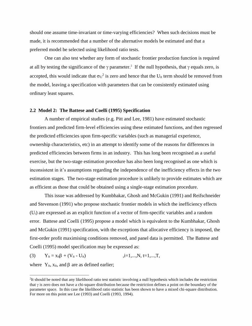
should one assume time-invariant or time-varying efficiencies? When such decisions must be
made, it is recommended that a number of the alternative models be estimated and that a
preferred model be selected using likelihood ratio tests.
One can also test whether any form of stochastic frontier production function is required
at all by testing the significance of the parameter.2 If the null hypothesis, that equals zero, is
accepted, this would indicate that U2 is zero and hence that the Uit term should be removed from
the model, leaving a specification with parameters that can be consistently estimated using
ordinary least squares.
2.2 Model 2: The Battese and Coelli (1995) Specification
A number of empirical studies (e.g. Pitt and Lee, 1981) have estimated stochastic
frontiers and predicted firm-level efficiencies using these estimated functions, and then regressed
the predicted efficiencies upon firm-specific variables (such as managerial experience,
ownership characteristics, etc) in an attempt to identify some of the reasons for differences in
predicted efficiencies between firms in an industry. This has long been recognised as a useful
exercise, but the two-stage estimation procedure has also been long recognised as one which is
inconsistent in it’s assumptions regarding the independence of the inefficiency effects in the two
estimation stages. The two-stage estimation procedure is unlikely to provide estimates which are
as efficient as those that could be obtained using a single-stage estimation procedure.
This issue was addressed by Kumbhakar, Ghosh and McGukin (1991) and Reifschneider
and Stevenson (1991) who propose stochastic frontier models in which the inefficiency effects
(Ui) are expressed as an explicit function of a vector of firm-specific variables and a random
error. Battese and Coelli (1995) propose a model which is equivalent to the Kumbhakar, Ghosh
and McGukin (1991) specification, with the exceptions that allocative efficiency is imposed, the
first-order profit maximising conditions removed, and panel data is permitted. The Battese and
Coelli (1995) model specification may be expressed as:
(3) Yit = xit + (Vit - Uit) ,i=1,...,N, t=1,...,T,
where Yit, xit, and are as defined earlier;
2It should be noted that any likelihood ratio test statistic involving a null hypothesis which includes the restriction
that is zero does not have a chi-square distribution because the restriction defines a point on the boundary of the
parameter space. In this case the likelihood ratio statistic has been shown to have a mixed chi-square distribution.
For more on this point see Lee (1993) and Coelli (1993, 1994).
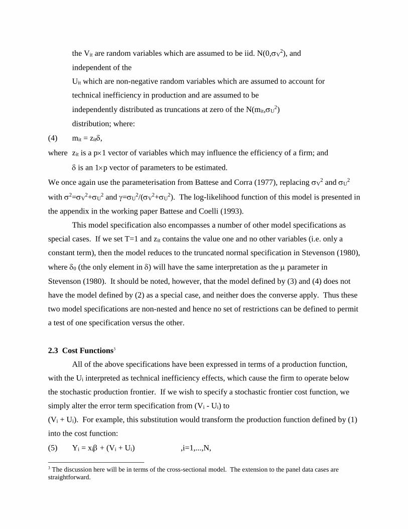
the Vit are random variables which are assumed to be iid. N(0,V2), and
independent of the
Uit which are non-negative random variables which are assumed to account for
technical inefficiency in production and are assumed to be
independently distributed as truncations at zero of the N(mit,U2)
distribution; where:
(4) mit = zit,
where zit is a p1 vector of variables which may influence the efficiency of a firm; and
is an 1p vector of parameters to be estimated.
We once again use the parameterisation from Battese and Corra (1977), replacing V2 and U
2
with 2=V2+U
2 and =U2/(V
2+U2). The log-likelihood function of this model is presented in
the appendix in the working paper Battese and Coelli (1993).
This model specification also encompasses a number of other model specifications as
special cases. If we set T=1 and zit contains the value one and no other variables (i.e. only a
constant term), then the model reduces to the truncated normal specification in Stevenson (1980),
where 0 (the only element in ) will have the same interpretation as the parameter in
Stevenson (1980). It should be noted, however, that the model defined by (3) and (4) does not
have the model defined by (2) as a special case, and neither does the converse apply. Thus these
two model specifications are non-nested and hence no set of restrictions can be defined to permit
a test of one specification versus the other.
2.3 Cost Functions3
All of the above specifications have been expressed in terms of a production function,
with the Ui interpreted as technical inefficiency effects, which cause the firm to operate below
the stochastic production frontier. If we wish to specify a stochastic frontier cost function, we
simply alter the error term specification from (Vi - Ui) to
(Vi + Ui). For example, this substitution would transform the production function defined by (1)
into the cost function:
(5) Yi = xi + (Vi + Ui) ,i=1,...,N,
3 The discussion here will be in terms of the cross-sectional model. The extension to the panel data cases are
straightforward.
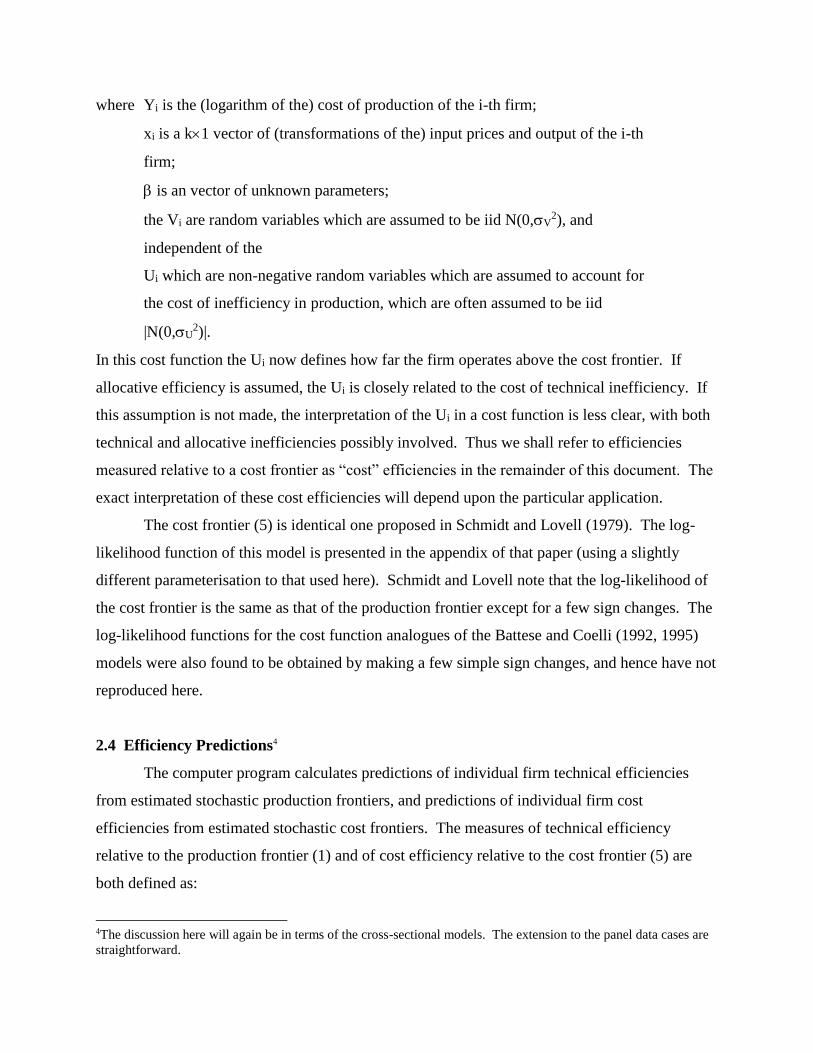
where Yi is the (logarithm of the) cost of production of the i-th firm;
xi is a k1 vector of (transformations of the) input prices and output of the i-th
firm;
is an vector of unknown parameters;
the Vi are random variables which are assumed to be iid N(0,V2), and
independent of the
Ui which are non-negative random variables which are assumed to account for
the cost of inefficiency in production, which are often assumed to be iid
|N(0,U2)|.
In this cost function the Ui now defines how far the firm operates above the cost frontier. If
allocative efficiency is assumed, the Ui is closely related to the cost of technical inefficiency. If
this assumption is not made, the interpretation of the Ui in a cost function is less clear, with both
technical and allocative inefficiencies possibly involved. Thus we shall refer to efficiencies
measured relative to a cost frontier as “cost” efficiencies in the remainder of this document. The
exact interpretation of these cost efficiencies will depend upon the particular application.
The cost frontier (5) is identical one proposed in Schmidt and Lovell (1979). The log-
likelihood function of this model is presented in the appendix of that paper (using a slightly
different parameterisation to that used here). Schmidt and Lovell note that the log-likelihood of
the cost frontier is the same as that of the production frontier except for a few sign changes. The
log-likelihood functions for the cost function analogues of the Battese and Coelli (1992, 1995)
models were also found to be obtained by making a few simple sign changes, and hence have not
reproduced here.
2.4 Efficiency Predictions4
The computer program calculates predictions of individual firm technical efficiencies
from estimated stochastic production frontiers, and predictions of individual firm cost
efficiencies from estimated stochastic cost frontiers. The measures of technical efficiency
relative to the production frontier (1) and of cost efficiency relative to the cost frontier (5) are
both defined as:
4The discussion here will again be in terms of the cross-sectional models. The extension to the panel data cases are
straightforward.
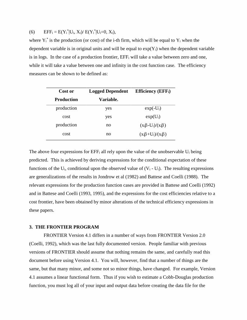
(6) EFFi = E(Yi*|Ui, Xi)/ E(Yi
*|Ui=0, Xi),
where Yi* is the production (or cost) of the i-th firm, which will be equal to Yi when the
dependent variable is in original units and will be equal to exp(Yi) when the dependent variable
is in logs. In the case of a production frontier, EFFi will take a value between zero and one,
while it will take a value between one and infinity in the cost function case. The efficiency
measures can be shown to be defined as:
Cost or
Production
Logged Dependent
Variable.
Efficiency (EFFi)
production yes exp(-Ui)
cost yes exp(Ui)
production no (xi-Ui)/(xi)
cost no (xi+Ui)/(xi)
The above four expressions for EFFi all rely upon the value of the unobservable Ui being
predicted. This is achieved by deriving expressions for the conditional expectation of these
functions of the Ui, conditional upon the observed value of (Vi - Ui). The resulting expressions
are generalizations of the results in Jondrow et al (1982) and Battese and Coelli (1988). The
relevant expressions for the production function cases are provided in Battese and Coelli (1992)
and in Battese and Coelli (1993, 1995), and the expressions for the cost efficiencies relative to a
cost frontier, have been obtained by minor alterations of the technical efficiency expressions in
these papers.
3. THE FRONTIER PROGRAM
FRONTIER Version 4.1 differs in a number of ways from FRONTIER Version 2.0
(Coelli, 1992), which was the last fully documented version. People familiar with previous
versions of FRONTIER should assume that nothing remains the same, and carefully read this
document before using Version 4.1. You will, however, find that a number of things are the
same, but that many minor, and some not so minor things, have changed. For example, Version
4.1 assumes a linear functional form. Thus if you wish to estimate a Cobb-Douglas production
function, you must log all of your input and output data before creating the data file for the
program to use. Version 2.0 users will recall that the Cobb-Douglas was assumed in that
version, and that data had to be supplied in original units, since the program obtained the logs of
the data supplied to it. A listing of the major differences between Versions 2.0 and 4.1 is
provided at the end of this section.
3.1 Files Needed
The execution of FRONTIER Version 4.1 on an IBM PC generally involves five files:
1) The executable file FRONT41.EXE
2) The start-up file FRONT41.000
3) A data file (for example, called TEST.DTA)
4) An instruction file (for example, called TEST.INS)
5) An output file (for example, called TEST.OUT).
The start-up file, FRONT41.000, contains values for a number of key variables such as the
convergence criterion, printing flags and so on. This text file may be edited if the user wishes to
alter any values. This file is discussed further in Appendix A. The data and instruction files
must be created by the user prior to execution. The output file is created by FRONTIER during
execution.5 Examples of a data, instruction and output files are listed in Section 4.
The program requires that the data be listed in an text file and is quite particular about the
format. The data must be listed by observation. There must be 3+k[+p] columns presented in
the following order:
1) Firm number (an integer in the range 1 to N)
2) Period number (an integer in the range 1 to T)
3) Yit
4) x1it
:
3+k) xkit
[3+k+1) z1it
:
3+k+p) zpit].
5Note that a model can be estimated without an instruction file if the program is used interactively.

The z entries are listed in square brackets to indicate that they are not always needed. They are
only used when Model 2 is being estimated. The observations can be listed in any order but the
columns must be in the stated order. There must be at least one observation on each of the N
firms and there must be at least one observation in time period 1 and in time period T. If you are
using a single cross-section of data, then column 2 (the time period column) should contain the
value “1” throughout. Note that the data must be suitably transformed if a functional form other
than a linear function is required. The Cobb-Douglas and Translog functional forms are the most
often used functional forms in stochastic frontier analyses. Examples involving these two forms
will be provided in Section 4.
The program can receive instructions either from a file or from a terminal. After typing
“FRONT41” to begin execution, the user is asked whether instructions will come from a file or
the terminal. The structure of the instruction file is listed in the next section. If the interactive
(terminal) option is selected, questions will be asked in the same order as they appear in the
instruction file.

3.2 The Three-Step Estimation Method
The program will follow a three-step procedure in estimating the maximum likelihood
estimates of the parameters of a stochastic frontier production function.6 The three steps are:
1) Ordinary Least Squares (OLS) estimates of the function are obtained. All
estimators with the exception of the intercept will be unbiased.
2) A two-phase grid search of is conducted, with the parameters (excepting
0) set to the OLS values and the 0 and 2 parameters adjusted
according to the corrected ordinary least squares formula presented in Coelli
(1995). Any other parameters (, or ‘s) are set to zero in this grid search.
3) The values selected in the grid search are used as starting values in an
iterative procedure (using the Davidon-Fletcher-Powell Quasi-Newton
method) to obtain the final maximum likelihood estimates.
3.2.1 Grid Search
As mentioned earlier, a grid search is conducted across the parameter space of . Values
of are considered from 0.1 to 0.9 in increments of size 0.1. The size of this increment can be
altered by changing the value of the GRIDNO variable which is set to the value of 0.1 in the
start-up file FRONT41.000.
Furthermore, if the variable, IGRID2, in FRONT41.000, is set to 1 (instead of 0) then a
second phase grid search will be conducted around the values obtained in the first phase. The
width of this grid search is GRIDNO/2 either side of the phase one estimates in steps of
GRIDNO/10. Thus a starting value for will be obtained to an accuracy of two decimal places
instead of the one decimal place obtained in the single phase grid search (when a value of
GRIDNO=0.1 is assumed).
3.2.2 Iterative Maximization Procedure
The first-order partial derivatives of the log-likelihood functions of Models 1 and 2 are
lengthy expressions. These are derived in appendices in Battese and Coelli (1992) and Battese
and Coelli (1993), respectively. Many of the gradient methods used to obtain maximum
6If starting values are specified in the instruction file, the program will skip the first two steps of the procedure.
likelihood estimates, such as the Newton-Raphson method, require the matrix of second partial
derivatives to be calculated. It was decided that this task was probably best avoided, hence we
turned our attention to Quasi-Newton methods which only require the vector of first partial
derivatives be derived. The Davidon-Fletcher-Powell Quasi-Newton method was selected as it
appears to have been used successfully in a wide range of econometric applications and was also
recommended by Pitt and Lee (1981) for stochastic frontier production function estimation. For
a general discussion of the relative merits of a number of Newton and Quasi-Newton methods
see Himmelblau (1972), which also provides a description of the mechanics (along with Fortran
code) of a number of the more popular methods. The general structure of the subroutines, MINI,
SEARCH, ETA and CONVRG, used in FRONTIER are taken from the appendix in Himmelblau
(1972).
The iterative procedure takes the parameter values supplied by the grid search as starting
values (unless starting values are supplied by the user). The program then updates the vector of
parameter estimates by the Davidon-Fletcher-Powell method until either of the following occurs:
a) The convergence criterion is satisfied. The convergence criterion is set in the start-
up file FRONT41.000 by the parameter TOL. Presently it is set such that, if the proportional
change in the likelihood function and each of the parameters is less than 0.00001, then the
iterative procedure terminates.
b) The maximum number of iterations permitted is completed. This is presently set in
FRONT41.000 to 100.
Both of these parameters may be altered by the user.
3.3 Program Output
The ordinary least-squares estimates, the estimates after the grid search and the final
maximum likelihood estimates are all presented in the output file. Approximate standard errors
are taken from the direction matrix used in the final iteration of the Davidon-Fletcher-Powell
procedure. This estimate of the covariance matrix is also listed in the output.
Estimates of individual technical or cost efficiencies are calculated using the expressions
presented in Battese and Coelli (1991, 1995). When any estimates of mean efficiencies are
reported, these are simply the arithmetic averages of the individual efficiencies. The ITE
variable in FRONT41.000 can be used to suppress the listing of individual efficiencies in the
output file, by changing it’s value from 1 to 0.
3.4 Differences Between Versions 2.0 and 4.1
The main differences are as follows:
1) The Battese and Coelli (1995) model (Model 2) can now be estimated.
2) The old size limits on N, T and K have been removed. The size limits of 100, 20 and 20,
respectively, were found by many users to be too restrictive. The removal of the size limits have
been achieved by compiling the program using a Lahey F77L-EM/32 compiler with a DOS
extender. The size of model that can now be estimated by the program is only limited by the
amount of the available RAM available on your PC. This action does come at some cost though,
since the program had to be re-written using dynamically allocatable arrays, which are not
standard Fortran constructs. Thus the code cannot now be transferred to another computing
platform (such as a mainframe computer) without substantial modification.
3) Cost functions can now be estimated.
4) Efficiency estimates can now be calculated when the dependent variable is expresses in
original units. The previous version of the program assumed the dependent variable was in logs,
and calculated efficiencies accordingly. The user can now indicate whether the dependent
variable is logged or not, and the program will then calculate the appropriate efficiency
estimates.
5) Version 2.0 was written to estimate a Cobb-Douglas function. Data was supplied in original
units and the program calculated the logs before estimation. Version 4.1 assumes that all
necessary transformations have already been done to the data before it receives it. The program
estimates a linear function using the data supplied to it. Examples of how to estimate Cobb-
Douglas and Translog functional forms are provided in Section 4.
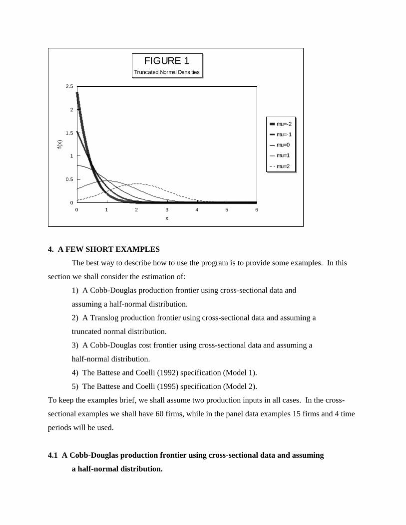
6) Bounds have now been placed upon the range of values that can take in Model 1. It is now
restricted to the range between 2U. This has been done because a number of users (including
the author) found that in some applications a large (insignificant) negative value of was
obtained. This value was large in the sense that it was many standard deviations from zero (e.g.
four or more). The numerical accuracy of calculations of areas in the tail of the standard normal
distribution which are this far from zero must be questioned.7 It was thus decided that the above
bounds be imposed. This was not viewed as being too restrictive, given the range of truncated
normal distribution shapes which are still permitted. This is evident in Figure 1 which plots
truncated normal density functions for values of of -2, -1, 0, 1 and 2
7) Information from each iteration is now sent to the output file (instead of to the screen). The
user can also now specify how often (if at all) this information is reported, using the IPRINT
variable in FRONT41.000.
8) The grid search has now been reduced to only consider and now uses the corrected ordinary
least squares expressions derived in Coelli (1995) to adjust 2 and 0 during this process.
9) A small error was detected in the first partial derivative with respect to in Version 2.0 of the
program. This error would have only affected results when was assumed to be non-zero. The
error has been corrected in Version 4.1, and the change does not appear to have a large influence
upon estimates.
10) As a result of the use of the new compiler (detailed under point 2), the following minimum
machine configuration is needed: an IBM compatible 386 (or higher) PC with a math co-
processor. The program will run when there is only 4 mb RAM but in some cases will require 8
mb RAM.
11) There have also been a large number of small alterations made to the program, many of
which were suggested by users of Version 2.0. For example, the names of the data and
instruction files are now listed in the output file.
7A monte carlo experiment was conducted in which was set to zero when generating samples, but was unrestricted
in estimation. Large negative (insignificant) values of were obtained in roughly 10% of samples. A 3D plot of the
log-likelihood function in one of these samples indicated a long flat ridge in the log-likelihood when plotted against
and 2. This phenomenon is being further investigated at present.
0 1 2 3 4 5 6
0
0.5
1
1.5
2
2.5
x
f(x)
mu=-2
mu=-1
mu=0
mu=1
mu=2
FIGURE 1Truncated Normal Densities
4. A FEW SHORT EXAMPLES
The best way to describe how to use the program is to provide some examples. In this
section we shall consider the estimation of:
1) A Cobb-Douglas production frontier using cross-sectional data and
assuming a half-normal distribution.
2) A Translog production frontier using cross-sectional data and assuming a
truncated normal distribution.
3) A Cobb-Douglas cost frontier using cross-sectional data and assuming a
half-normal distribution.
4) The Battese and Coelli (1992) specification (Model 1).
5) The Battese and Coelli (1995) specification (Model 2).
To keep the examples brief, we shall assume two production inputs in all cases. In the cross-
sectional examples we shall have 60 firms, while in the panel data examples 15 firms and 4 time
periods will be used.
4.1 A Cobb-Douglas production frontier using cross-sectional data and assuming
a half-normal distribution.
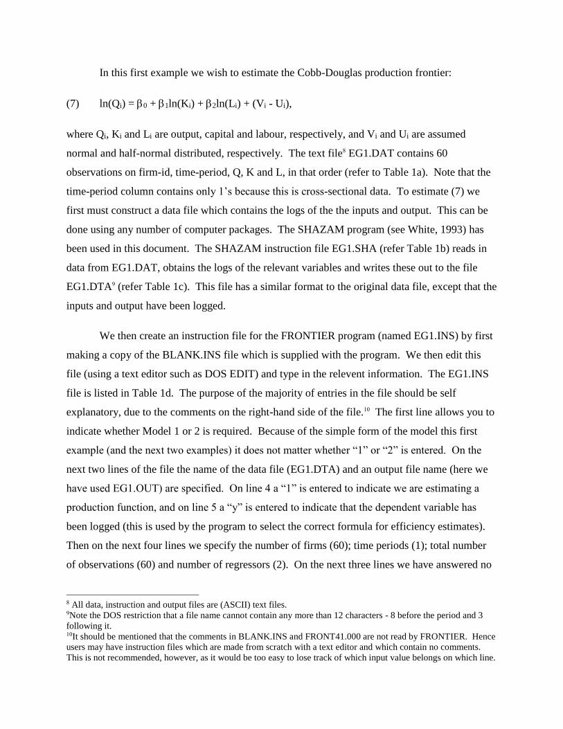
In this first example we wish to estimate the Cobb-Douglas production frontier:
(7) ln(Qi) = 0 + 1ln(Ki) + 2ln(Li) + (Vi - Ui),
where Qi, Ki and Li are output, capital and labour, respectively, and Vi and Ui are assumed
normal and half-normal distributed, respectively. The text file8 EG1.DAT contains 60
observations on firm-id, time-period, Q, K and L, in that order (refer to Table 1a). Note that the
time-period column contains only 1’s because this is cross-sectional data. To estimate (7) we
first must construct a data file which contains the logs of the the inputs and output. This can be
done using any number of computer packages. The SHAZAM program (see White, 1993) has
been used in this document. The SHAZAM instruction file EG1.SHA (refer Table 1b) reads in
data from EG1.DAT, obtains the logs of the relevant variables and writes these out to the file
EG1.DTA9 (refer Table 1c). This file has a similar format to the original data file, except that the
inputs and output have been logged.
We then create an instruction file for the FRONTIER program (named EG1.INS) by first
making a copy of the BLANK.INS file which is supplied with the program. We then edit this
file (using a text editor such as DOS EDIT) and type in the relevent information. The EG1.INS
file is listed in Table 1d. The purpose of the majority of entries in the file should be self
explanatory, due to the comments on the right-hand side of the file.10 The first line allows you to
indicate whether Model 1 or 2 is required. Because of the simple form of the model this first
example (and the next two examples) it does not matter whether “1” or “2” is entered. On the
next two lines of the file the name of the data file (EG1.DTA) and an output file name (here we
have used EG1.OUT) are specified. On line 4 a “1” is entered to indicate we are estimating a
production function, and on line 5 a “y” is entered to indicate that the dependent variable has
been logged (this is used by the program to select the correct formula for efficiency estimates).
Then on the next four lines we specify the number of firms (60); time periods (1); total number
of observations (60) and number of regressors (2). On the next three lines we have answered no
8 All data, instruction and output files are (ASCII) text files. 9Note the DOS restriction that a file name cannot contain any more than 12 characters - 8 before the period and 3
following it. 10It should be mentioned that the comments in BLANK.INS and FRONT41.000 are not read by FRONTIER. Hence
users may have instruction files which are made from scratch with a text editor and which contain no comments.
This is not recommended, however, as it would be too easy to lose track of which input value belongs on which line.
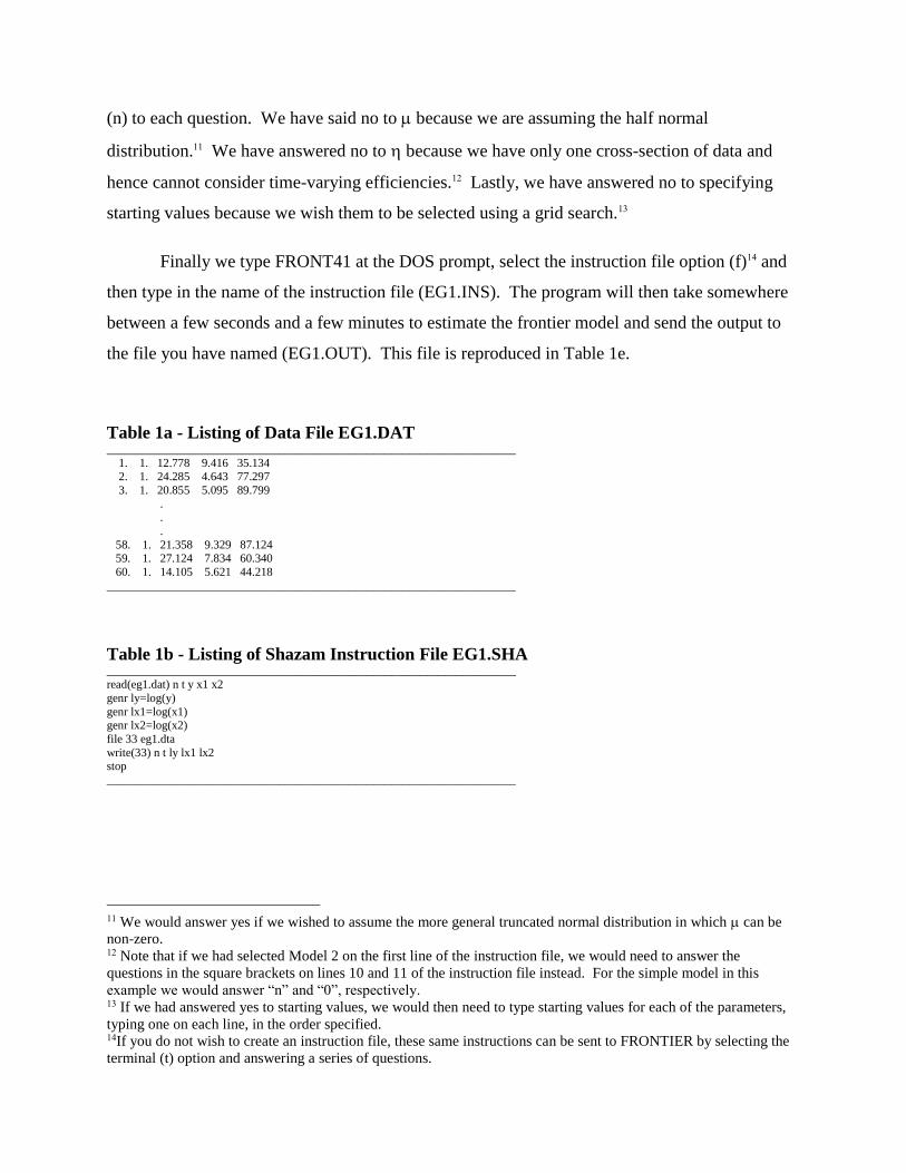
(n) to each question. We have said no to because we are assuming the half normal
distribution.11 We have answered no to because we have only one cross-section of data and
hence cannot consider time-varying efficiencies.12 Lastly, we have answered no to specifying
starting values because we wish them to be selected using a grid search.13
Finally we type FRONT41 at the DOS prompt, select the instruction file option (f)14 and
then type in the name of the instruction file (EG1.INS). The program will then take somewhere
between a few seconds and a few minutes to estimate the frontier model and send the output to
the file you have named (EG1.OUT). This file is reproduced in Table 1e.
Table 1a - Listing of Data File EG1.DAT _____________________________________________________________________
1. 1. 12.778 9.416 35.134 2. 1. 24.285 4.643 77.297
3. 1. 20.855 5.095 89.799
. .
.
58. 1. 21.358 9.329 87.124 59. 1. 27.124 7.834 60.340
60. 1. 14.105 5.621 44.218
_____________________________________________________________________
Table 1b - Listing of Shazam Instruction File EG1.SHA _____________________________________________________________________ read(eg1.dat) n t y x1 x2
genr ly=log(y)
genr lx1=log(x1) genr lx2=log(x2)
file 33 eg1.dta
write(33) n t ly lx1 lx2 stop
_____________________________________________________________________
11 We would answer yes if we wished to assume the more general truncated normal distribution in which can be
non-zero. 12 Note that if we had selected Model 2 on the first line of the instruction file, we would need to answer the
questions in the square brackets on lines 10 and 11 of the instruction file instead. For the simple model in this
example we would answer “n” and “0”, respectively. 13 If we had answered yes to starting values, we would then need to type starting values for each of the parameters,
typing one on each line, in the order specified. 14If you do not wish to create an instruction file, these same instructions can be sent to FRONTIER by selecting the
terminal (t) option and answering a series of questions.
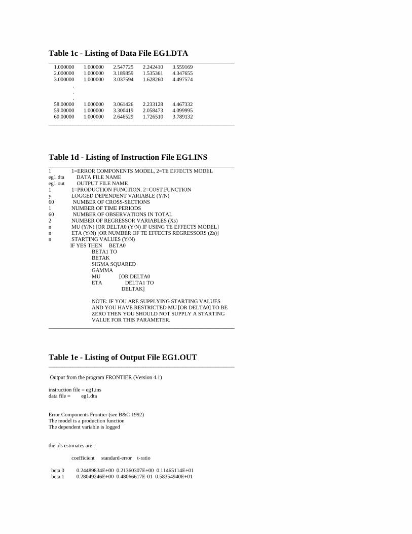
Table 1c - Listing of Data File EG1.DTA _____________________________________________________________________
1.000000 1.000000 2.547725 2.242410 3.559169 2.000000 1.000000 3.189859 1.535361 4.347655
3.000000 1.000000 3.037594 1.628260 4.497574
. .
.
58.00000 1.000000 3.061426 2.233128 4.467332 59.00000 1.000000 3.300419 2.058473 4.099995
60.00000 1.000000 2.646529 1.726510 3.789132
_____________________________________________________________________
Table 1d - Listing of Instruction File EG1.INS _____________________________________________________________________
1 1=ERROR COMPONENTS MODEL, 2=TE EFFECTS MODEL eg1.dta DATA FILE NAME
eg1.out OUTPUT FILE NAME
1 1=PRODUCTION FUNCTION, 2=COST FUNCTION y LOGGED DEPENDENT VARIABLE (Y/N)
60 NUMBER OF CROSS-SECTIONS
1 NUMBER OF TIME PERIODS 60 NUMBER OF OBSERVATIONS IN TOTAL
2 NUMBER OF REGRESSOR VARIABLES (Xs)
n MU (Y/N) [OR DELTA0 (Y/N) IF USING TE EFFECTS MODEL] n ETA (Y/N) [OR NUMBER OF TE EFFECTS REGRESSORS (Zs)]
n STARTING VALUES (Y/N)
IF YES THEN BETA0 BETA1 TO
BETAK
SIGMA SQUARED GAMMA
MU [OR DELTA0
ETA DELTA1 TO DELTAK]
NOTE: IF YOU ARE SUPPLYING STARTING VALUES AND YOU HAVE RESTRICTED MU [OR DELTA0] TO BE
ZERO THEN YOU SHOULD NOT SUPPLY A STARTING
VALUE FOR THIS PARAMETER. _____________________________________________________________________
Table 1e - Listing of Output File EG1.OUT _____________________________________________________________________
Output from the program FRONTIER (Version 4.1)
instruction file = eg1.ins
data file = eg1.dta
Error Components Frontier (see B&C 1992) The model is a production function
The dependent variable is logged
the ols estimates are :
coefficient standard-error t-ratio
beta 0 0.24489834E+00 0.21360307E+00 0.11465114E+01 beta 1 0.28049246E+00 0.48066617E-01 0.58354940E+01
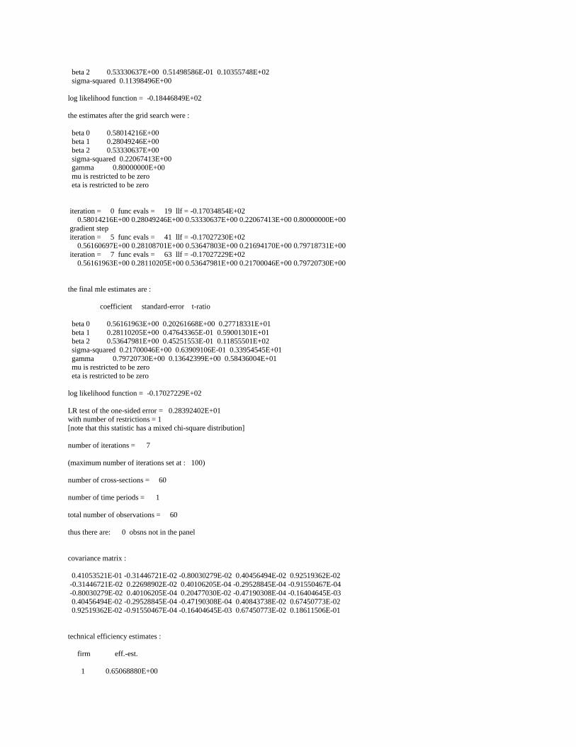
beta 2 0.53330637E+00 0.51498586E-01 0.10355748E+02
sigma-squared 0.11398496E+00
log likelihood function = -0.18446849E+02
the estimates after the grid search were :
beta 0 0.58014216E+00 beta 1 0.28049246E+00
beta 2 0.53330637E+00
sigma-squared 0.22067413E+00 gamma 0.80000000E+00
mu is restricted to be zero
eta is restricted to be zero
iteration = 0 func evals = 19 llf = -0.17034854E+02 0.58014216E+00 0.28049246E+00 0.53330637E+00 0.22067413E+00 0.80000000E+00
gradient step
iteration = 5 func evals = 41 llf = -0.17027230E+02 0.56160697E+00 0.28108701E+00 0.53647803E+00 0.21694170E+00 0.79718731E+00
iteration = 7 func evals = 63 llf = -0.17027229E+02
0.56161963E+00 0.28110205E+00 0.53647981E+00 0.21700046E+00 0.79720730E+00
the final mle estimates are :
coefficient standard-error t-ratio
beta 0 0.56161963E+00 0.20261668E+00 0.27718331E+01
beta 1 0.28110205E+00 0.47643365E-01 0.59001301E+01 beta 2 0.53647981E+00 0.45251553E-01 0.11855501E+02
sigma-squared 0.21700046E+00 0.63909106E-01 0.33954545E+01
gamma 0.79720730E+00 0.13642399E+00 0.58436004E+01 mu is restricted to be zero
eta is restricted to be zero
log likelihood function = -0.17027229E+02
LR test of the one-sided error = 0.28392402E+01 with number of restrictions = 1
[note that this statistic has a mixed chi-square distribution]
number of iterations = 7
(maximum number of iterations set at : 100)
number of cross-sections = 60
number of time periods = 1
total number of observations = 60
thus there are: 0 obsns not in the panel
covariance matrix :
0.41053521E-01 -0.31446721E-02 -0.80030279E-02 0.40456494E-02 0.92519362E-02
-0.31446721E-02 0.22698902E-02 0.40106205E-04 -0.29528845E-04 -0.91550467E-04
-0.80030279E-02 0.40106205E-04 0.20477030E-02 -0.47190308E-04 -0.16404645E-03 0.40456494E-02 -0.29528845E-04 -0.47190308E-04 0.40843738E-02 0.67450773E-02
0.92519362E-02 -0.91550467E-04 -0.16404645E-03 0.67450773E-02 0.18611506E-01
technical efficiency estimates :
firm eff.-est.
1 0.65068880E+00
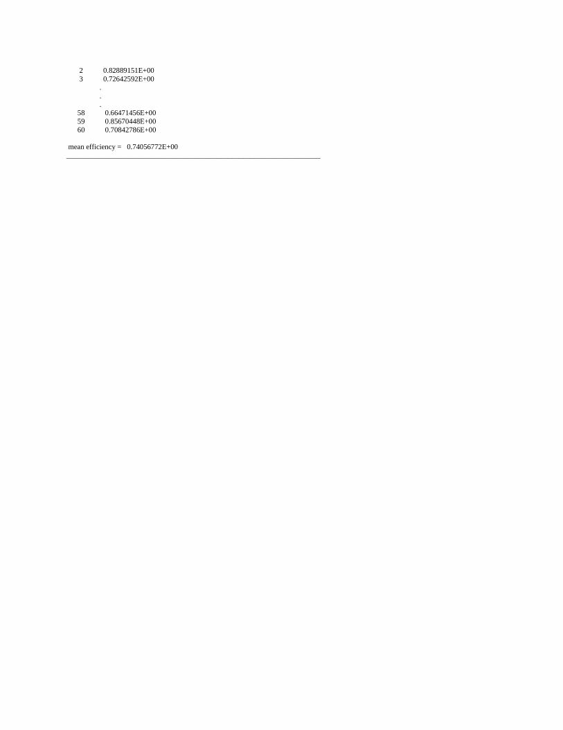
2 0.82889151E+00
3 0.72642592E+00 .
.
. 58 0.66471456E+00
59 0.85670448E+00
60 0.70842786E+00
mean efficiency = 0.74056772E+00
_____________________________________________________________________
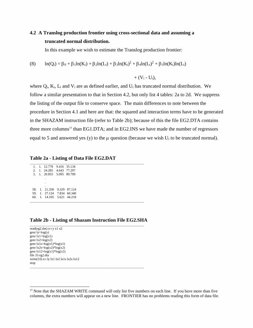
4.2 A Translog production frontier using cross-sectional data and assuming a
truncated normal distribution.
In this example we wish to estimate the Translog production frontier:
(8) ln(Qi) = 0 + 1ln(Ki) + 2ln(Li) + 3ln(Ki)2 + 4ln(Li)
2 + 5ln(Ki)ln(Li)
+ (Vi - Ui),
where Qi, Ki, Li and Vi are as defined earlier, and Ui has truncated normal distribution. We
follow a similar presentation to that in Section 4.2, but only list 4 tables: 2a to 2d. We suppress
the listing of the output file to conserve space. The main differences to note between the
procedure in Section 4.1 and here are that: the squared and interaction terms have to be generated
in the SHAZAM instruction file (refer to Table 2b); because of this the file EG2.DTA contains
three more columns15 than EG1.DTA; and in EG2.INS we have made the number of regressors
equal to 5 and answered yes (y) to the question (because we wish Ui to be truncated normal).
Table 2a - Listing of Data File EG2.DAT _____________________________________________________________________
1. 1. 12.778 9.416 35.134
2. 1. 24.285 4.643 77.297
3. 1. 20.855 5.095 89.799
.
. .
58. 1. 21.358 9.329 87.124
59. 1. 27.124 7.834 60.340 60. 1. 14.105 5.621 44.218
_____________________________________________________________________
Table 2b - Listing of Shazam Instruction File EG2.SHA _____________________________________________________________________
read(eg2.dat) n t y x1 x2 genr ly=log(y)
genr lx1=log(x1)
genr lx2=log(x2)
genr lx1s=log(x1)*log(x1)
genr lx2s=log(x2)*log(x2)
genr lx12=log(x1)*log(x2) file 33 eg2.dta
write(33) n t ly lx1 lx2 lx1s lx2s lx12
stop _____________________________________________________________________
15 Note that the SHAZAM WRITE command will only list five numbers on each line. If you have more than five
columns, the extra numbers will appear on a new line. FRONTIER has no problems reading this form of data file.
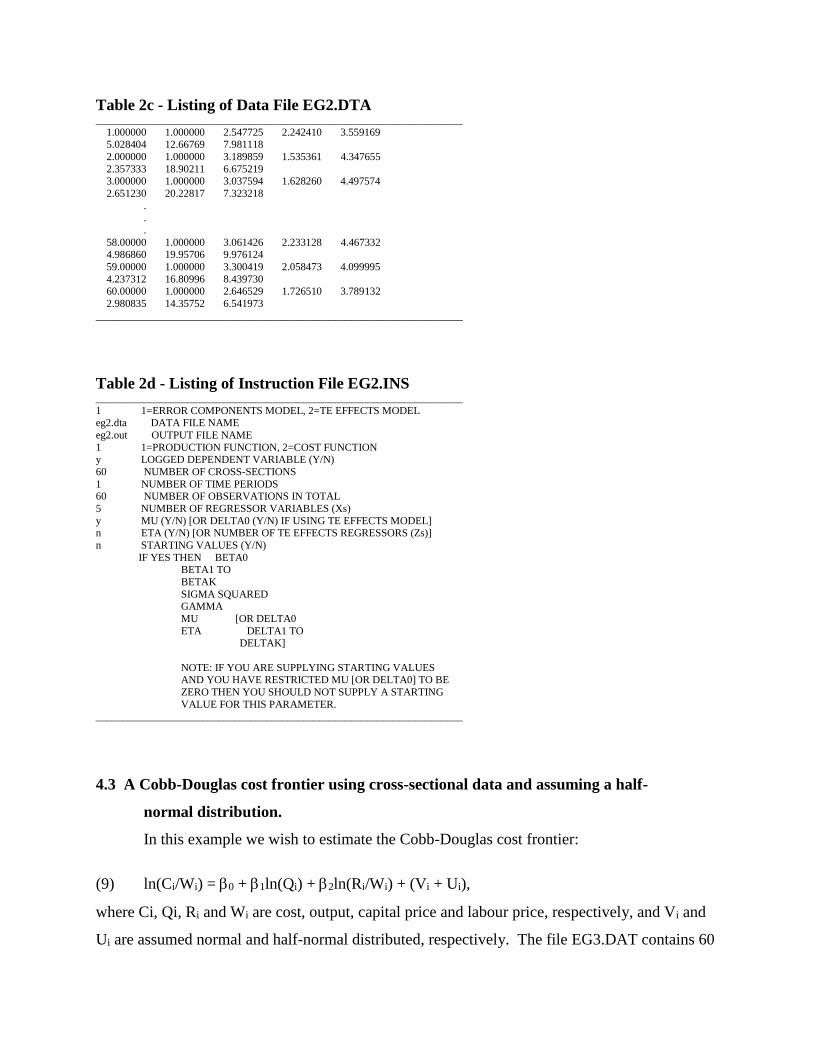
Table 2c - Listing of Data File EG2.DTA _____________________________________________________________________
1.000000 1.000000 2.547725 2.242410 3.559169 5.028404 12.66769 7.981118
2.000000 1.000000 3.189859 1.535361 4.347655
2.357333 18.90211 6.675219 3.000000 1.000000 3.037594 1.628260 4.497574
2.651230 20.22817 7.323218
. .
.
58.00000 1.000000 3.061426 2.233128 4.467332 4.986860 19.95706 9.976124
59.00000 1.000000 3.300419 2.058473 4.099995
4.237312 16.80996 8.439730 60.00000 1.000000 2.646529 1.726510 3.789132
2.980835 14.35752 6.541973
_____________________________________________________________________
Table 2d - Listing of Instruction File EG2.INS _____________________________________________________________________
1 1=ERROR COMPONENTS MODEL, 2=TE EFFECTS MODEL eg2.dta DATA FILE NAME
eg2.out OUTPUT FILE NAME
1 1=PRODUCTION FUNCTION, 2=COST FUNCTION y LOGGED DEPENDENT VARIABLE (Y/N)
60 NUMBER OF CROSS-SECTIONS
1 NUMBER OF TIME PERIODS 60 NUMBER OF OBSERVATIONS IN TOTAL
5 NUMBER OF REGRESSOR VARIABLES (Xs)
y MU (Y/N) [OR DELTA0 (Y/N) IF USING TE EFFECTS MODEL] n ETA (Y/N) [OR NUMBER OF TE EFFECTS REGRESSORS (Zs)]
n STARTING VALUES (Y/N)
IF YES THEN BETA0 BETA1 TO
BETAK
SIGMA SQUARED GAMMA
MU [OR DELTA0
ETA DELTA1 TO DELTAK]
NOTE: IF YOU ARE SUPPLYING STARTING VALUES AND YOU HAVE RESTRICTED MU [OR DELTA0] TO BE
ZERO THEN YOU SHOULD NOT SUPPLY A STARTING
VALUE FOR THIS PARAMETER. _____________________________________________________________________
4.3 A Cobb-Douglas cost frontier using cross-sectional data and assuming a half-
normal distribution.
In this example we wish to estimate the Cobb-Douglas cost frontier:
(9) ln(Ci/Wi) = 0 + 1ln(Qi) + 2ln(Ri/Wi) + (Vi + Ui),
where Ci, Qi, Ri and Wi are cost, output, capital price and labour price, respectively, and Vi and
Ui are assumed normal and half-normal distributed, respectively. The file EG3.DAT contains 60
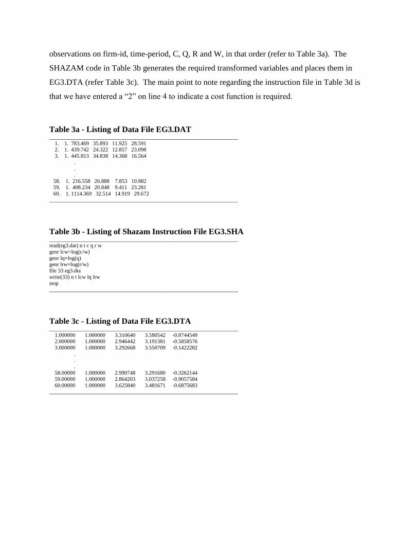
observations on firm-id, time-period, C, Q, R and W, in that order (refer to Table 3a). The
SHAZAM code in Table 3b generates the required transformed variables and places them in
EG3.DTA (refer Table 3c). The main point to note regarding the instruction file in Table 3d is
that we have entered a “2” on line 4 to indicate a cost function is required.
Table 3a - Listing of Data File EG3.DAT _____________________________________________________________________
1. 1. 783.469 35.893 11.925 28.591 2. 1. 439.742 24.322 12.857 23.098
3. 1. 445.813 34.838 14.368 16.564
. .
.
58. 1. 216.558 26.888 7.853 10.882 59. 1. 408.234 20.848 9.411 23.281
60. 1. 1114.369 32.514 14.919 29.672
_____________________________________________________________________
Table 3b - Listing of Shazam Instruction File EG3.SHA _____________________________________________________________________ read(eg3.dat) n t c q r w
genr lcw=log(c/w)
genr lq=log(q) genr lrw=log(r/w)
file 33 eg3.dta
write(33) n t lcw lq lrw stop
_____________________________________________________________________
Table 3c - Listing of Data File EG3.DTA _____________________________________________________________________
1.000000 1.000000 3.310640 3.580542 -0.8744549 2.000000 1.000000 2.946442 3.191381 -0.5858576
3.000000 1.000000 3.292668 3.550709 -0.1422282
. .
.
58.00000 1.000000 2.990748 3.291680 -0.3262144 59.00000 1.000000 2.864203 3.037258 -0.9057584
60.00000 1.000000 3.625840 3.481671 -0.6875683
_____________________________________________________________________
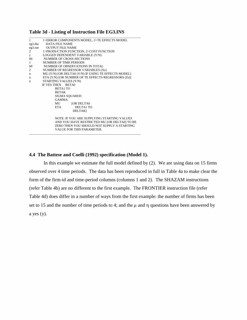
Table 3d - Listing of Instruction File EG3.INS _____________________________________________________________________
1 1=ERROR COMPONENTS MODEL, 2=TE EFFECTS MODEL eg3.dta DATA FILE NAME
eg3.out OUTPUT FILE NAME
2 1=PRODUCTION FUNCTION, 2=COST FUNCTION y LOGGED DEPENDENT VARIABLE (Y/N)
60 NUMBER OF CROSS-SECTIONS
1 NUMBER OF TIME PERIODS 60 NUMBER OF OBSERVATIONS IN TOTAL
2 NUMBER OF REGRESSOR VARIABLES (Xs)
n MU (Y/N) [OR DELTA0 (Y/N) IF USING TE EFFECTS MODEL] n ETA (Y/N) [OR NUMBER OF TE EFFECTS REGRESSORS (Zs)]
n STARTING VALUES (Y/N)
IF YES THEN BETA0 BETA1 TO
BETAK
SIGMA SQUARED GAMMA
MU [OR DELTA0
ETA DELTA1 TO DELTAK]
NOTE: IF YOU ARE SUPPLYING STARTING VALUES AND YOU HAVE RESTRICTED MU [OR DELTA0] TO BE
ZERO THEN YOU SHOULD NOT SUPPLY A STARTING VALUE FOR THIS PARAMETER.
_____________________________________________________________________
4.4 The Battese and Coelli (1992) specification (Model 1).
In this example we estimate the full model defined by (2). We are using data on 15 firms
observed over 4 time periods. The data has been reproduced in full in Table 4a to make clear the
form of the firm-id and time-period columns (columns 1 and 2). The SHAZAM instructions
(refer Table 4b) are no different to the first example. The FRONTIER instruction file (refer
Table 4d) does differ in a number of ways from the first example: the number of firms has been
set to 15 and the number of time periods to 4; and the and questions have been answered by
a yes (y).
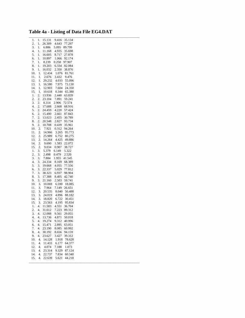
Table 4a - Listing of Data File EG4.DAT _____________________________________________________________________
1. 1. 15.131 9.416 35.134 2. 1. 26.309 4.643 77.297
3. 1. 6.886 5.095 89.799
4. 1. 11.168 4.935 35.698 5. 1. 16.605 8.717 27.878
6. 1. 10.897 1.066 92.174
7. 1. 8.239 0.258 97.907 8. 1. 19.203 6.334 82.084
9. 1. 16.032 2.350 38.876
10. 1. 12.434 1.076 81.761 11. 1. 2.676 3.432 9.476
12. 1. 29.232 4.033 55.096
13. 1. 16.580 7.975 73.130 14. 1. 12.903 7.604 24.350
15. 1. 10.618 0.344 65.380
1. 2. 13.936 2.440 63.839 2. 2. 23.104 7.891 59.241
3. 2. 8.314 2.906 72.574
4. 2. 17.688 2.668 68.916 5. 2. 24.459 4.220 57.424
6. 2. 15.490 2.661 87.843
7. 2. 13.023 2.455 30.789 8. 2. 20.548 2.827 93.734
9. 2. 10.708 0.439 35.961 10. 2. 7.921 0.312 94.264
11. 2. 14.966 3.265 95.773
12. 2. 25.989 6.752 80.275 13. 2. 14.264 4.425 49.886
14. 2. 9.690 1.583 22.072
15. 2. 9.034 0.907 38.727 1. 3. 5.379 6.149 5.322
2. 3. 2.498 0.479 2.520
3. 3. 7.884 1.955 41.545 4. 3. 24.334 8.169 68.389
5. 3. 19.668 4.055 77.556
6. 3. 22.337 5.029 77.812 7. 3. 38.323 6.937 98.904
8. 3. 17.388 8.405 42.740
9. 3. 21.160 2.503 59.741 10. 3. 10.069 6.590 18.085
11. 3. 7.964 7.149 26.651
12. 3. 20.535 8.040 50.488 13. 3. 24.019 4.896 88.182
14. 3. 18.820 6.722 30.451
15. 3. 23.563 4.195 95.834 1. 4. 11.583 4.551 36.704
2. 4. 31.612 7.223 89.312
3. 4. 12.088 9.561 29.055 4. 4. 13.736 4.871 50.018
5. 4. 19.274 9.312 40.996
6. 4. 15.471 2.895 63.051 7. 4. 23.190 8.085 60.992
8. 4. 30.192 8.656 94.159
9. 4. 23.627 3.427 39.312 10. 4. 14.128 1.918 78.628
11. 4. 11.433 6.177 64.377
12. 4. 4.074 7.188 1.073 13. 4. 23.314 9.329 87.124
14. 4. 22.737 7.834 60.340
15. 4. 22.639 5.621 44.218 _____________________________________________________________________
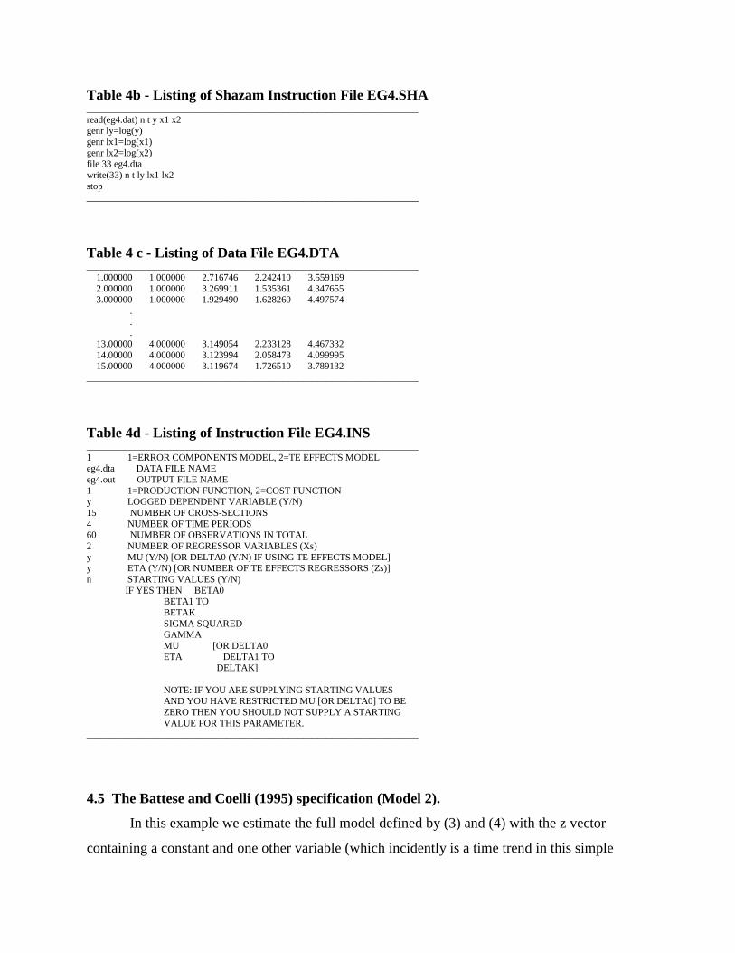
Table 4b - Listing of Shazam Instruction File EG4.SHA _____________________________________________________________________
read(eg4.dat) n t y x1 x2 genr ly=log(y)
genr lx1=log(x1)
genr lx2=log(x2) file 33 eg4.dta
write(33) n t ly lx1 lx2
stop _____________________________________________________________________
Table 4 c - Listing of Data File EG4.DTA _____________________________________________________________________
1.000000 1.000000 2.716746 2.242410 3.559169
2.000000 1.000000 3.269911 1.535361 4.347655 3.000000 1.000000 1.929490 1.628260 4.497574
.
. .
13.00000 4.000000 3.149054 2.233128 4.467332
14.00000 4.000000 3.123994 2.058473 4.099995 15.00000 4.000000 3.119674 1.726510 3.789132
_____________________________________________________________________
Table 4d - Listing of Instruction File EG4.INS _____________________________________________________________________
1 1=ERROR COMPONENTS MODEL, 2=TE EFFECTS MODEL eg4.dta DATA FILE NAME
eg4.out OUTPUT FILE NAME
1 1=PRODUCTION FUNCTION, 2=COST FUNCTION y LOGGED DEPENDENT VARIABLE (Y/N)
15 NUMBER OF CROSS-SECTIONS
4 NUMBER OF TIME PERIODS 60 NUMBER OF OBSERVATIONS IN TOTAL
2 NUMBER OF REGRESSOR VARIABLES (Xs)
y MU (Y/N) [OR DELTA0 (Y/N) IF USING TE EFFECTS MODEL] y ETA (Y/N) [OR NUMBER OF TE EFFECTS REGRESSORS (Zs)]
n STARTING VALUES (Y/N)
IF YES THEN BETA0 BETA1 TO
BETAK
SIGMA SQUARED GAMMA
MU [OR DELTA0
ETA DELTA1 TO DELTAK]
NOTE: IF YOU ARE SUPPLYING STARTING VALUES AND YOU HAVE RESTRICTED MU [OR DELTA0] TO BE
ZERO THEN YOU SHOULD NOT SUPPLY A STARTING
VALUE FOR THIS PARAMETER. _____________________________________________________________________
4.5 The Battese and Coelli (1995) specification (Model 2).
In this example we estimate the full model defined by (3) and (4) with the z vector
containing a constant and one other variable (which incidently is a time trend in this simple
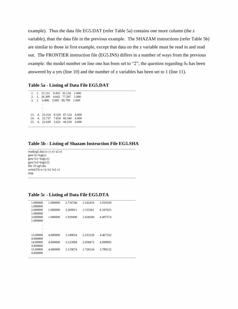
example). Thus the data file EG5.DAT (refer Table 5a) contains one more column (the z
variable), than the data file in the previous example. The SHAZAM instructions (refer Table 5b)
are similar to those in first example, except that data on the z variable must be read in and read
out. The FRONTIER instruction file (EG5.INS) differs in a number of ways from the previous
example: the model number on line one has been set to “2”; the question regarding 0 has been
answered by a yes (line 10) and the number of z variables has been set to 1 (line 11).
Table 5a - Listing of Data File EG5.DAT _____________________________________________________________________
1. 1. 15.131 9.416 35.134 1.000 2. 1. 26.309 4.643 77.297 1.000
3. 1. 6.886 5.095 89.799 1.000
. .
.
13. 4. 23.314 9.329 87.124 4.000 14. 4. 22.737 7.834 60.340 4.000
15. 4. 22.639 5.621 44.218 4.000
_____________________________________________________________________
Table 5b - Listing of Shazam Instruction File EG5.SHA _____________________________________________________________________
read(eg5.dat) n t y x1 x2 z1 genr ly=log(y)
genr lx1=log(x1)
genr lx2=log(x2)
file 33 eg5.dta
write(33) n t ly lx1 lx2 z1
stop _____________________________________________________________________
Table 5c - Listing of Data File EG5.DTA _____________________________________________________________________
1.000000 1.000000 2.716746 2.242410 3.559169
1.000000 2.000000 1.000000 3.269911 1.535361 4.347655
1.000000
3.000000 1.000000 1.929490 1.628260 4.497574 1.000000
.
.
.
13.00000 4.000000 3.149054 2.233128 4.467332
4.000000 14.00000 4.000000 3.123994 2.058473 4.099995
4.000000
15.00000 4.000000 3.119674 1.726510 3.789132 4.000000
_____________________________________________________________________
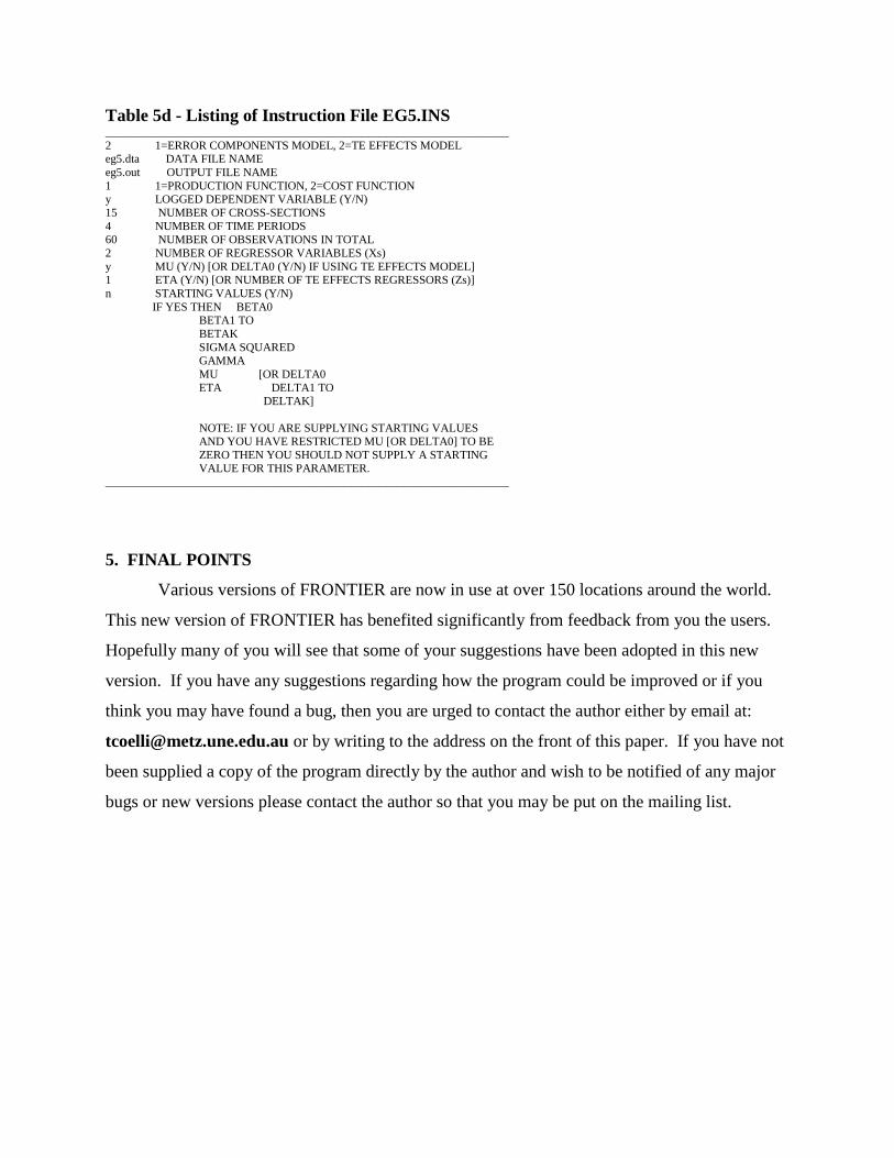
Table 5d - Listing of Instruction File EG5.INS _____________________________________________________________________
2 1=ERROR COMPONENTS MODEL, 2=TE EFFECTS MODEL eg5.dta DATA FILE NAME
eg5.out OUTPUT FILE NAME
1 1=PRODUCTION FUNCTION, 2=COST FUNCTION y LOGGED DEPENDENT VARIABLE (Y/N)
15 NUMBER OF CROSS-SECTIONS
4 NUMBER OF TIME PERIODS 60 NUMBER OF OBSERVATIONS IN TOTAL
2 NUMBER OF REGRESSOR VARIABLES (Xs)
y MU (Y/N) [OR DELTA0 (Y/N) IF USING TE EFFECTS MODEL] 1 ETA (Y/N) [OR NUMBER OF TE EFFECTS REGRESSORS (Zs)]
n STARTING VALUES (Y/N)
IF YES THEN BETA0 BETA1 TO
BETAK
SIGMA SQUARED GAMMA
MU [OR DELTA0
ETA DELTA1 TO DELTAK]
NOTE: IF YOU ARE SUPPLYING STARTING VALUES AND YOU HAVE RESTRICTED MU [OR DELTA0] TO BE
ZERO THEN YOU SHOULD NOT SUPPLY A STARTING VALUE FOR THIS PARAMETER.
_____________________________________________________________________
5. FINAL POINTS
Various versions of FRONTIER are now in use at over 150 locations around the world.
This new version of FRONTIER has benefited significantly from feedback from you the users.
Hopefully many of you will see that some of your suggestions have been adopted in this new
version. If you have any suggestions regarding how the program could be improved or if you
think you may have found a bug, then you are urged to contact the author either by email at:
[email protected] or by writing to the address on the front of this paper. If you have not
been supplied a copy of the program directly by the author and wish to be notified of any major
bugs or new versions please contact the author so that you may be put on the mailing list.
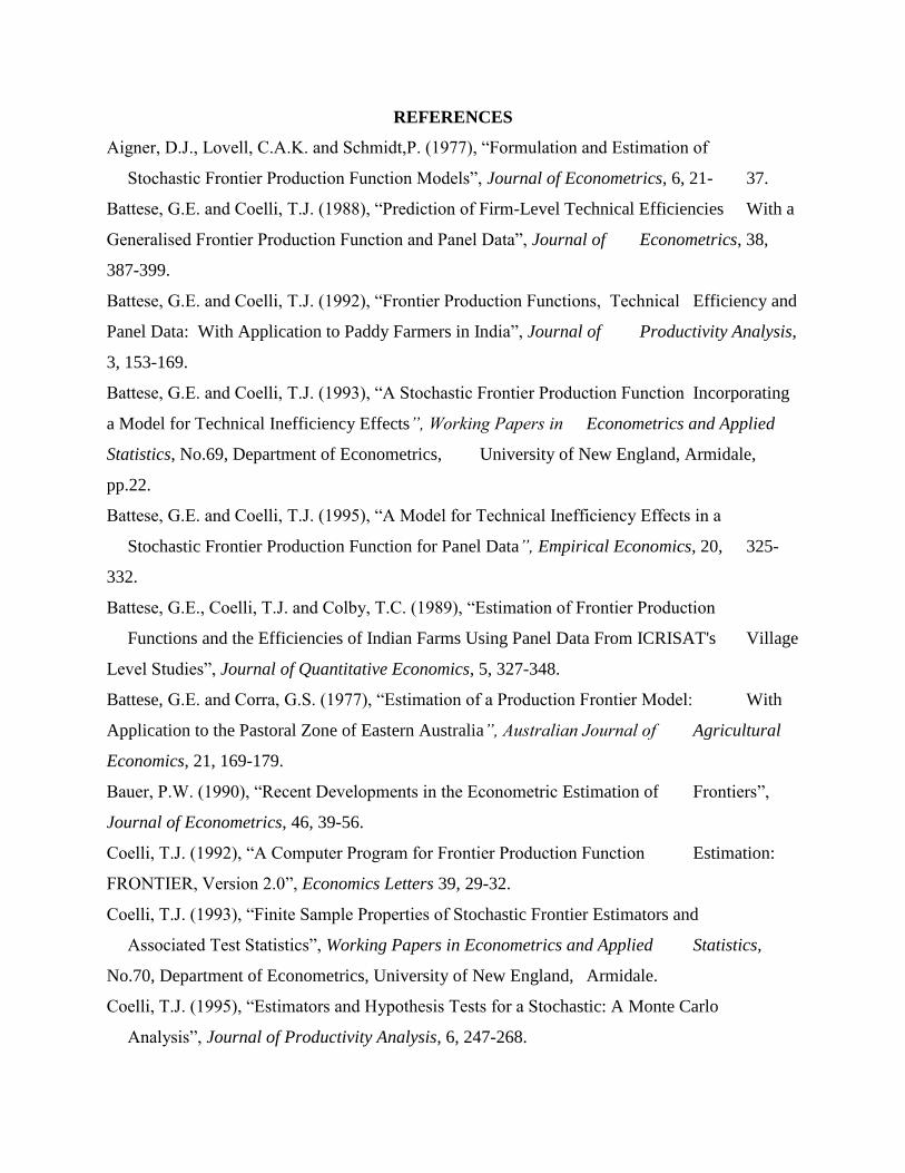
REFERENCES
Aigner, D.J., Lovell, C.A.K. and Schmidt,P. (1977), “Formulation and Estimation of
Stochastic Frontier Production Function Models”, Journal of Econometrics, 6, 21- 37.
Battese, G.E. and Coelli, T.J. (1988), “Prediction of Firm-Level Technical Efficiencies With a
Generalised Frontier Production Function and Panel Data”, Journal of Econometrics, 38,
387-399.
Battese, G.E. and Coelli, T.J. (1992), “Frontier Production Functions, Technical Efficiency and
Panel Data: With Application to Paddy Farmers in India”, Journal of Productivity Analysis,
3, 153-169.
Battese, G.E. and Coelli, T.J. (1993), “A Stochastic Frontier Production Function Incorporating
a Model for Technical Inefficiency Effects”, Working Papers in Econometrics and Applied
Statistics, No.69, Department of Econometrics, University of New England, Armidale,
pp.22.
Battese, G.E. and Coelli, T.J. (1995), “A Model for Technical Inefficiency Effects in a
Stochastic Frontier Production Function for Panel Data”, Empirical Economics, 20, 325-
332.
Battese, G.E., Coelli, T.J. and Colby, T.C. (1989), “Estimation of Frontier Production
Functions and the Efficiencies of Indian Farms Using Panel Data From ICRISAT's Village
Level Studies”, Journal of Quantitative Economics, 5, 327-348.
Battese, G.E. and Corra, G.S. (1977), “Estimation of a Production Frontier Model: With
Application to the Pastoral Zone of Eastern Australia”, Australian Journal of Agricultural
Economics, 21, 169-179.
Bauer, P.W. (1990), “Recent Developments in the Econometric Estimation of Frontiers”,
Journal of Econometrics, 46, 39-56.
Coelli, T.J. (1992), “A Computer Program for Frontier Production Function Estimation:
FRONTIER, Version 2.0”, Economics Letters 39, 29-32.
Coelli, T.J. (1993), “Finite Sample Properties of Stochastic Frontier Estimators and
Associated Test Statistics”, Working Papers in Econometrics and Applied Statistics,
No.70, Department of Econometrics, University of New England, Armidale.
Coelli, T.J. (1995), “Estimators and Hypothesis Tests for a Stochastic: A Monte Carlo
Analysis”, Journal of Productivity Analysis, 6, 247-268.
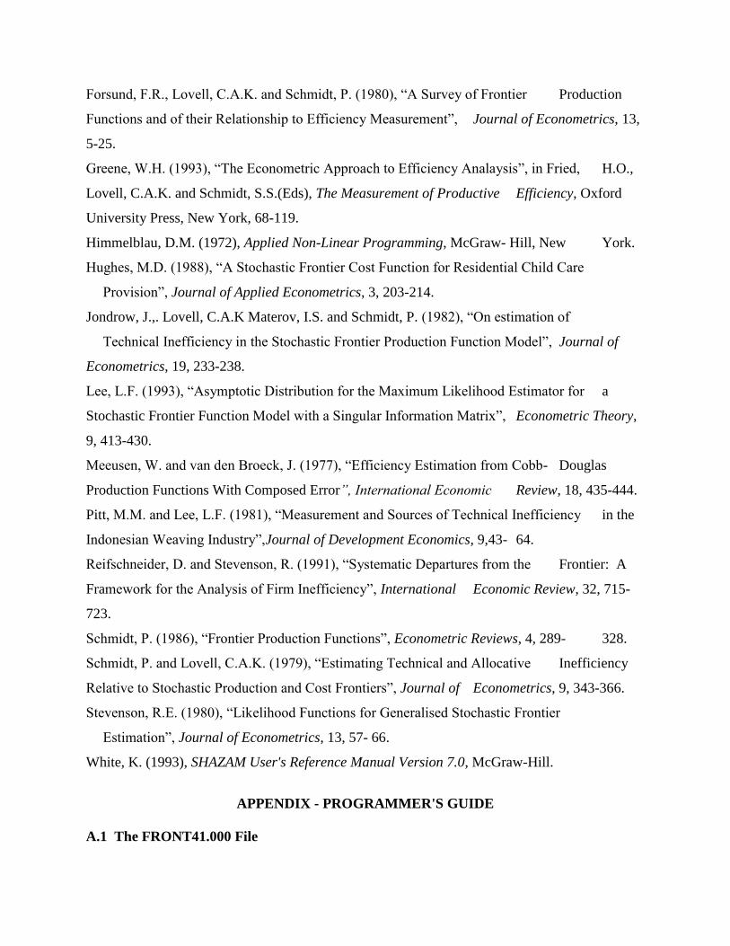
Forsund, F.R., Lovell, C.A.K. and Schmidt, P. (1980), “A Survey of Frontier Production
Functions and of their Relationship to Efficiency Measurement”, Journal of Econometrics, 13,
5-25.
Greene, W.H. (1993), “The Econometric Approach to Efficiency Analaysis”, in Fried, H.O.,
Lovell, C.A.K. and Schmidt, S.S.(Eds), The Measurement of Productive Efficiency, Oxford
University Press, New York, 68-119.
Himmelblau, D.M. (1972), Applied Non-Linear Programming, McGraw- Hill, New York.
Hughes, M.D. (1988), “A Stochastic Frontier Cost Function for Residential Child Care
Provision”, Journal of Applied Econometrics, 3, 203-214.
Jondrow, J.,. Lovell, C.A.K Materov, I.S. and Schmidt, P. (1982), “On estimation of
Technical Inefficiency in the Stochastic Frontier Production Function Model”, Journal of
Econometrics, 19, 233-238.
Lee, L.F. (1993), “Asymptotic Distribution for the Maximum Likelihood Estimator for a
Stochastic Frontier Function Model with a Singular Information Matrix”, Econometric Theory,
9, 413-430.
Meeusen, W. and van den Broeck, J. (1977), “Efficiency Estimation from Cobb- Douglas
Production Functions With Composed Error”, International Economic Review, 18, 435-444.
Pitt, M.M. and Lee, L.F. (1981), “Measurement and Sources of Technical Inefficiency in the
Indonesian Weaving Industry”,Journal of Development Economics, 9,43- 64.
Reifschneider, D. and Stevenson, R. (1991), “Systematic Departures from the Frontier: A
Framework for the Analysis of Firm Inefficiency”, International Economic Review, 32, 715-
723.
Schmidt, P. (1986), “Frontier Production Functions”, Econometric Reviews, 4, 289- 328.
Schmidt, P. and Lovell, C.A.K. (1979), “Estimating Technical and Allocative Inefficiency
Relative to Stochastic Production and Cost Frontiers”, Journal of Econometrics, 9, 343-366.
Stevenson, R.E. (1980), “Likelihood Functions for Generalised Stochastic Frontier
Estimation”, Journal of Econometrics, 13, 57- 66.
White, K. (1993), SHAZAM User's Reference Manual Version 7.0, McGraw-Hill.
APPENDIX - PROGRAMMER'S GUIDE
A.1 The FRONT41.000 File
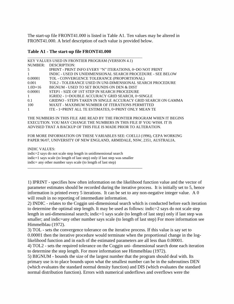
The start-up file FRONT41.000 is listed in Table A1. Ten values may be altered in
FRONT41.000. A brief description of each value is provided below.
Table A1 - The start-up file FRONT41.000 ____________________________________________________________
KEY VALUES USED IN FRONTIER PROGRAM (VERSION 4.1)
NUMBER: DESCRIPTION:
5 IPRINT - PRINT INFO EVERY “N” ITERATIONS, 0=DO NOT PRINT
1 INDIC - USED IN UNIDIMENSIONAL SEARCH PROCEDURE - SEE BELOW
0.00001 TOL - CONVERGENCE TOLERANCE (PROPORTIONAL)
0.001 TOL2 - TOLERANCE USED IN UNI-DIMENSIONAL SEARCH PROCEDURE
1.0D+16 BIGNUM - USED TO SET BOUNDS ON DEN & DIST
0.00001 STEP1 - SIZE OF 1ST STEP IN SEARCH PROCEDURE
1 IGRID2 - 1=DOUBLE ACCURACY GRID SEARCH, 0=SINGLE
0.1 GRIDNO - STEPS TAKEN IN SINGLE ACCURACY GRID SEARCH ON GAMMA
100 MAXIT - MAXIMUM NUMBER OF ITERATIONS PERMITTED
1 ITE - 1=PRINT ALL TE ESTIMATES, 0=PRINT ONLY MEAN TE
THE NUMBERS IN THIS FILE ARE READ BY THE FRONTIER PROGRAM WHEN IT BEGINS
EXECUTION. YOU MAY CHANGE THE NUMBERS IN THIS FILE IF YOU WISH. IT IS
ADVISED THAT A BACKUP OF THIS FILE IS MADE PRIOR TO ALTERATION.
FOR MORE INFORMATION ON THESE VARIABLES SEE: COELLI (1996), CEPA WORKING
PAPER 96/07, UNIVERSITY OF NEW ENGLAND, ARMIDALE, NSW, 2351, AUSTRALIA.
INDIC VALUES:
indic=2 says do not scale step length in unidimensional search
indic=1 says scale (to length of last step) only if last step was smaller
indic= any other number says scale (to length of last step)
____________________________________________________________
1) IPRINT - specifies how often information on the likelihood function value and the vector of
parameter estimates should be recorded during the iterative process. It is initially set to 5, hence
information is printed every 5 iterations. It can be set to any non-negative integer value. A 0
will result in no reporting of intermediate information.
2) INDIC - relates to the Coggin uni-dimensional search which is conducted before each iteration
to determine the optimal step length. It may be used as follows: indic=2 says do not scale step
length in uni-dimensional search; indic=1 says scale (to length of last step) only if last step was
smaller; and indic=any other number says scale (to length of last step) For more information see
Himmelblau (1972).
3) TOL - sets the convergence tolerance on the iterative process. If this value is say set to
0.00001 then the iterative procedure would terminate when the proportional change in the log-
likelihood function and in each of the estimated parameters are all less than 0.00001.
4) TOL2 - sets the required tolerance on the Coggin uni- dimensional search done each iteration
to determine the step length. For more information see Himmelblau (1972).
5) BIGNUM - bounds the size of the largest number that the program should deal with. Its
primary use is to place bounds upon what the smallest number can be in the subroutines DEN
(which evaluates the standard normal density function) and DIS (which evaluates the standard
normal distribution function). Errors with numerical underflows and overflows were the
problems most frequently encountered by people attempting to install earlier versions of this
program on various mainframe computers. This number has been set to 1.0e+16 for the IBM PC.
If you plan to mount this program on a mainframe computer it is advised that you consult
computer support staff on the correct setting of this number. It generally would be safe to leave it
as it is, however, greater precision may be gained if larger numbers are permitted.
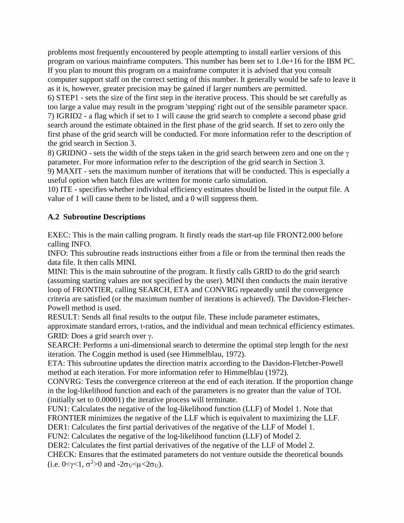
6) STEP1 - sets the size of the first step in the iterative process. This should be set carefully as
too large a value may result in the program 'stepping' right out of the sensible parameter space.
7) IGRID2 - a flag which if set to 1 will cause the grid search to complete a second phase grid
search around the estimate obtained in the first phase of the grid search. If set to zero only the
first phase of the grid search will be conducted. For more information refer to the description of
the grid search in Section 3.
8) GRIDNO - sets the width of the steps taken in the grid search between zero and one on the
parameter. For more information refer to the description of the grid search in Section 3.
9) MAXIT - sets the maximum number of iterations that will be conducted. This is especially a
useful option when batch files are written for monte carlo simulation.
10) ITE - specifies whether individual efficiency estimates should be listed in the output file. A
value of 1 will cause them to be listed, and a 0 will suppress them.
A.2 Subroutine Descriptions
EXEC: This is the main calling program. It firstly reads the start-up file FRONT2.000 before
calling INFO.
INFO: This subroutine reads instructions either from a file or from the terminal then reads the
data file. It then calls MINI.
MINI: This is the main subroutine of the program. It firstly calls GRID to do the grid search
(assuming starting values are not specified by the user). MINI then conducts the main iterative
loop of FRONTIER, calling SEARCH, ETA and CONVRG repeatedly until the convergence
criteria are satisfied (or the maximum number of iterations is achieved). The Davidon-Fletcher-
Powell method is used.
RESULT: Sends all final results to the output file. These include parameter estimates,
approximate standard errors, t-ratios, and the individual and mean technical efficiency estimates.
GRID: Does a grid search over .
SEARCH: Performs a uni-dimensional search to determine the optimal step length for the next
iteration. The Coggin method is used (see Himmelblau, 1972).
ETA: This subroutine updates the direction matrix according to the Davidon-Fletcher-Powell
method at each iteration. For more information refer to Himmelblau (1972).
CONVRG: Tests the convergence critereon at the end of each iteration. If the proportion change
in the log-likelihood function and each of the parameters is no greater than the value of TOL
(initially set to 0.00001) the iterative process will terminate.
FUN1: Calculates the negative of the log-likelihood function (LLF) of Model 1. Note that
FRONTIER minimizes the negative of the LLF which is equivalent to maximizing the LLF.
DER1: Calculates the first partial derivatives of the negative of the LLF of Model 1.
FUN2: Calculates the negative of the log-likelihood function (LLF) of Model 2.
DER2: Calculates the first partial derivatives of the negative of the LLF of Model 2.
CHECK: Ensures that the estimated parameters do not venture outside the theoretical bounds
(i.e. 0<<1, 2>0 and -2U<<2U).
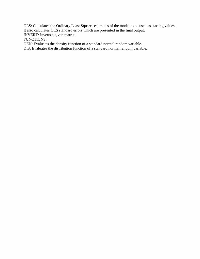
OLS: Calculates the Ordinary Least Squares estimates of the model to be used as starting values.
It also calculates OLS standard errors which are presented in the final output.
INVERT: Inverts a given matrix.
FUNCTIONS:
DEN: Evaluates the density function of a standard normal random variable.
DIS: Evaluates the distribution function of a standard normal random variable.
Related Documents