Noname manuscript No. (will be inserted by the editor) A computational comparison between Isogeometric Analysis and Spectral Element Methods: accuracy and spectral properties Paola Gervasio · Luca Ded` e · Ondine Chanon · Alfio Quarteroni the date of receipt and acceptance should be inserted later Abstract In this paper, we carry out a systematic comparison between the theo- retical properties of Spectral Element Methods (SEM) and NURBS–based Isoge- ometric Analysis (IGA) in its basic form, that is in the framework of the Galerkin method, for the approximation of the Poisson problem, which we select as a bench- mark Partial Differential Equation. Our focus is on their convergence properties, the algebraic structure and the spectral properties of the corresponding discrete arrays (mass and stiffness matrices). We review the available theoretical results for these methods and verify them numerically by performing an error analysis on the solution of the Poisson problem. Where theory is lacking, we use numerical inves- tigation of the results to draw conjectures on the behaviour of the corresponding theoretical laws in terms of the design parameters, such as the (mesh) element size, the local polynomial degree, the smoothness of the NURBS basis functions, the space dimension, and the total number of degrees of freedom involved in the computations. Keywords isogeometric analysis, spectral element methods, rate of convergence, condition number, computational comparison P. Gervasio DICATAM, Universit`a degli Studi di Brescia, via Branze 38, I-25123 Brescia, Italy L. Ded` e MOX, Department of Mathematics, Politecnico di Milano, Piazza Leonardo da Vinci 32, 20133 Milano, Italy O. Chanon MNS, Institute of Mathematics, ´ Ecole Polytechnique F´ ed´ erale de Lausanne, Station 8, CH- 1015 Lausanne, Switzerland A. Quarteroni MOX, Department of Mathematics, Politecnico di Milano, Piazza Leonardo da Vinci 32, 20133 Milano, Italy, and Institute of Mathematics, ´ Ecole Polytechnique F´ ed´ erale de Lausanne (EPFL), Station 8, CH-1015 Lausanne, Switzerland (honorary professor)

Welcome message from author
This document is posted to help you gain knowledge. Please leave a comment to let me know what you think about it! Share it to your friends and learn new things together.
Transcript
Noname manuscript No.(will be inserted by the editor)
A computational comparison between IsogeometricAnalysis and Spectral Element Methods: accuracy andspectral properties
Paola Gervasio · Luca Dede · Ondine
Chanon · Alfio Quarteroni
the date of receipt and acceptance should be inserted later
Abstract In this paper, we carry out a systematic comparison between the theo-retical properties of Spectral Element Methods (SEM) and NURBS–based Isoge-ometric Analysis (IGA) in its basic form, that is in the framework of the Galerkinmethod, for the approximation of the Poisson problem, which we select as a bench-mark Partial Differential Equation. Our focus is on their convergence properties,the algebraic structure and the spectral properties of the corresponding discretearrays (mass and stiffness matrices). We review the available theoretical results forthese methods and verify them numerically by performing an error analysis on thesolution of the Poisson problem. Where theory is lacking, we use numerical inves-tigation of the results to draw conjectures on the behaviour of the correspondingtheoretical laws in terms of the design parameters, such as the (mesh) elementsize, the local polynomial degree, the smoothness of the NURBS basis functions,the space dimension, and the total number of degrees of freedom involved in thecomputations.
Keywords isogeometric analysis, spectral element methods, rate of convergence,condition number, computational comparison
P. GervasioDICATAM, Universita degli Studi di Brescia, via Branze 38, I-25123 Brescia, Italy
L. DedeMOX, Department of Mathematics, Politecnico di Milano, Piazza Leonardo da Vinci 32, 20133Milano, Italy
O. ChanonMNS, Institute of Mathematics, Ecole Polytechnique Federale de Lausanne, Station 8, CH-1015 Lausanne, Switzerland
A. QuarteroniMOX, Department of Mathematics, Politecnico di Milano, Piazza Leonardo da Vinci 32,20133 Milano, Italy, and Institute of Mathematics, Ecole Polytechnique Federale de Lausanne(EPFL), Station 8, CH-1015 Lausanne, Switzerland (honorary professor)
2 Paola Gervasio et al.
1 Introduction
Spectral element methods (SEM) (see, e.g., [14]) and Isogeometric Analysis (IGA)(see, e.g., [15]) can be seen as two different paradigms for high order approximationof partial differential equations (PDEs); as a matter of fact, albeit IGA was notoriginally introduced with this aim, employing specific basis functions may leadto interpret it as an high order method. Apart from their different use of basisfunctions, piecewise polynomials for SEM, B–spline or NURBS for IGA (withvariable degree of continuity across element boundaries), the two approaches sharemany similarities. The perhaps more remarkable are reported below:
1 – they can be both recast in the framework of the Galerkin method: SEMis however most often used with inexact calculation of integrals using the so-called Gauss-Legendre-Lobatto numerical integration. This results into the so-called SEM-NI method (NI standing for numerical integration), which is the onewe address in this paper. On the other side, for IGA, we consider the so calledNURBS-based IGA in the framework of the Galerkin method. While we are wellaware that several efforts have been recently successfully made to improve theefficiency of IGA – especially for the reduction of assembly costs through thedevelopment of quadrature formulas tailored for NURBS [11,2,33,6,7,45], as wellas of partial tensor decompositions [43,36,46,1,6], and above all by means of IGAcollocation methods [24,39,3,29,40,44,4,42,19,22] – we decided here to stick tothe basic version of the method, which is still the most widespread one;
2 – the induced approximation error decays more than algebraically fast withrespect to the local polynomial degree.
On the other hand, the two methods differ in what concerns the algebraicstructures of the corresponding arrays (say, the mass and the stiffness matrices),the spectral properties of the latter (the behaviour of their extreme eigenvalues,and the corresponding condition number), and the actual decay rate of the ap-proximation error with respect to the discretization parameters: the element-sizeh, and the local polynomial degree p.
Our aim in this note is to report the most relevant theoretical results addressingthe aforementioned issues. Most of the results on the rate of convergence of theapproximation error are taken from the existing literature (see, e.g. [9,10,13,14,8,17,18]) and reorganise some of them for a better exploitation in our comparison.However, few of them are new. When the theory is missing we investigate theseproperties numerically and we propose the law of behaviour in terms of h, p, thespatial dimension d, and the total number of degrees of freedom (dof).
Our analysis is concerned with the approximation of the mass matrix and thestiffness matrix for the Poisson boundary value problem in a cubic domain. Wesystematically compare SEM-NI with two realisations of IGA: IGA-C0 (only thecontinuity across interelement boundaries is imposed on the problem solution, i.e.the NURBS basis functions are only globally C0-continuous in the computationaldomain) and IGA-Cp−1 (the continuity holds for the solution as well as for allits derivatives of order up to p − 1, i.e. the NURBS basis functions are globallyCp−1-continuous in the computational domain).
In general terms we can conclude that, errorwise, IGA-C0 and SEM-NI behaveessentially in the same way. For instance, their rate of convergence with respect toh scales (optimally) as p in the H1−norm, and (p+1) in the L2− norm. IGA-Cp−1
exhibits the same type of convergence, even if the errors it produces are larger than
Comparing IGA and SEM: accuracy and spectral properties 3
those provided by IGA-C0 and SEM-NI with the same values of h and p, basicallydue to the (much) lower number of dofs involved in the discretization for the samevalue of h. When h is kept fixed and p is increased, IGA-C0 and SEM-NI convergewith a rate that is only dictated by the Sobolev regularity of the solution (henceexponentially fast in case the latter is analytical). The same is true for IGA-Cp−1,although with a slower rate of decay. IGA-Cp−1 provides however the lowest errorwhen the three methods are run with the same number of degrees of freedom.
On a different side, SEM-NI arrays are in general less dense and better condi-tioned than those of IGA-Cp−1. In particular, SEM-NI minimises the error withrespect to the number of non-zero entries of the stiffness matrix (those that under-mine the computational cost of the stiffness matrix assembling and of the matrix-vector products for residual evaluations in iterative methods).
In the second part of the paper, the spectral analysis concerning the behaviourof the extreme eigenvalues (and associated condition number) of IGA arrays (massand stiffness matrices) complements the rather scarce literature available on thesubject. More precisely starting from the numerical computation of the extremeeigenvalues for any spatial dimension d = 1, 2, 3, we mimic (with analytic laws)the real behaviour of the spectral condition number of the IGA matrices againstthe local polynomial degree p and the element-size h.
While it is well known (see, e.g., [9,38,13,14]) that the condition number ofthe SEM-NI stiffness matrix grows algebraically as h−2p3 for all h and p, theanalysis of the present paper highlights that the spectral condition number of theIGA-C0 stiffness matrix grows algebraically like h−2p2 when h is sufficiently smallw.r.t. p and exponentially like p−d/24dp otherwise; moreover, the spectral conditionnumber of the IGA-Cp−1 stiffness matrix grows algebraically like h−2p when h issufficiently small w.r.t. p and exponentially, at least like pedp, otherwise.
The condition number of the SEM-NI mass matrix grows algebraically like pd,while we find that the condition numbers of the IGA mass matrices (either IGA-C0
and IGA-Cp−1) grow exponentially with p.The moduli of the extreme eigenvalues are examined also for the 1D advection-
diffusion operator for different values of the Peclet number in either elliptic oradvective regimes.
A specific outline of the paper is as follows.In Section 2 we present the Poisson problem, its discretization by SEM-NI (in
particular we describe how to deal with curved boundaries in the SEM contextfor d = 2 and d = 3 by exploiting transfinite mappings) and by IGA methods,then we resume the theoretical convergence estimates for both the approaches. InSection 3 we compare the numerical convergence rates of the methods when theyare applied to solve the Poisson problem with given solution. In the first test casewe solve the differential problem on the cube domain with either SEM-NI, IGA-C0 and IGA-Cp−1. In the second one we consider a more general domain withcurved boundary and compare the convergence curves of SEM-NI and IGA-Cp−1
approximations, as well as the CPUtimes needed to assemble the stiffness matrices.Section 4 is devoted to the spectral analysis of both the mass matrix and thestiffness matrix for the Poisson problem. After reviewing theoretical results knownin literature, we present our conjectures (based on the numerical computations ofextreme eigenvalues) about the behaviour of the spectral condition number of IGAmatrices versus both p and h. Finally, Section 5 deals with the spectral analysisof the 1D advection-diffusion stiffness matrices.
4 Paola Gervasio et al.
This review addresses for the first time a systematic comparison of the the-oretical properties of two classes of methods that are very popular and highlyappreciated in the community of numerical analysts and computational scientists.We are confident that this analysis will be useful for a comparative assessment ofthe two approaches and a better awareness of their strengths and limitations.
2 Problem setting
Let Ω ⊂ Rd, with d = 1, 2, 3, be a bounded domain (when d ≥ 2 we require thatthe boundary ∂Ω is Lipschitz continuous), and let f ∈ L2(Ω) be a given function.Our reference Poisson problem, which we use through most of the paper as abenchmark problem, reads
−∆u = f in Ω
u = 0 on ∂Ω.(1)
The weak form of problem (1) reads: find u ∈ V = H10 (Ω) such that
a(u, v) = F(v) ∀v ∈ V, (2)
where a(u, v) =
∫Ω
∇u · ∇v dΩ and F(v) =
∫Ω
fv dΩ. Problem (2) admits a
unique solution (see, e.g., [41]) that is stable w.r.t. the datum f . The case ofnon-homogeneous Dirichlet data leads back to the homogeneous case by standardarguments.
2.1 Discretization by the Spectral Element Method (SEM)
Given h > 0, let Th be a family of partitions of the computational domain Ω ⊂ Rdin neh quads (intervals when d = 1, quadrilaterals when d = 2, and hexahedra whend = 3). Following standard assumptions we require Th to be conformal, regular,and quasi-uniform (see [41, Ch. 3]). We denote by T the reference element, i.e.the d−dimensional cube (−1, 1)d and let each element T` ∈ Th be the image of thereference element T through a sufficiently smooth one-to-one map F` : T → T`with a sufficiently smooth inverse F−1
` : T` → T . If F` is affine, then the elementT` is a parallelogram (when d = 2) or a parallelepipedon (when d = 3).
To deal with more general domains, also in the case of curved boundaries, weconsider transfinite mappings introduced in [30–32].
So far, each element can be viewed as the image of a transfinite map Fk; inorder to guarantee the conformity of the mesh, if Tk and Tm share a common edgeor a face, say Γkm, then Fk and Fm must agree there, i.e. Fk|Γkm ≡ Fm|Γkm .
Formulation. Given an integer p ≥ 1, let us denote by Qp the space of polynomialsof degree less than or equal to p with respect to each direction in Ω ⊂ Rd. Weintroduce the following finite dimensional spaces in Ω: Xδ = v ∈ C0(Ω) : v|Tk ∈Qp F−1
k , ∀Tk ∈ Th, Vδ = V ∩ Xδ = v ∈ Xδ : v|∂Ω = 0. The index δ is anabridged notation undermining the mesh size h and the local polynomial degree p.
Comparing IGA and SEM: accuracy and spectral properties 5
The Galerkin approximation of (2) reads: find uδ ∈ Vδ such that
a(uδ, vδ) = F(vδ), ∀vδ ∈ Vδ.
Typically, when using SEM, the exact integrals appearing in a and F arereplaced by the composite Legendre–Gauss–Lobatto (LGL) quadrature formulas(see [13]) with the aim of reducing the computational effort. This is exactly theapproach that we consider in this paper, i.e the so called SEM with NumericalIntegration (SEM-NI) at the LGL nodes [14].
For any integer p ≥ 1, the (p+ 1) LGL nodes and weights are first defined onthe reference interval [−1, 1] (see [13, formula (2.3.12)]) and then tensorized andmapped into the generic quad T` ∈ Th by applying the transfinite map F`. Letx`,q and w`,q, with q = 1, . . . , (p + 1)d, denote the quadrature nodes and weightson T` for any T` ∈ Th and let neh be the number of elements in Th. For anyu, v ∈ L2(Ω) such that u, v ∈ C0(T`) for any T` ∈ Th, we define the compositeLegendre–Gauss–Lobatto-Legendre quadrature formula
(u, v)δ =
neh∑`=1
(p+1)d∑q=1
u(x`,q) · v(x`,q)w`,q. (3)
Then, for any uδ, vδ ∈ Xδ and f ∈ L2(Ω) such that f|T` ∈ C0(T`), we setaδ(uδ, vδ) = (∇uδ,∇vδ)δ and Fδ(vδ) = (f, vδ)δ.
The discrete Galerkin formulation of (2) with Numerical Integration (SEM-NI)reads: find uδ ∈ Vδ such that
aδ(uδ, vδ) = Fδ(vδ) ∀vδ ∈ Vδ. (4)
Algebraic form. Le us denote by N = N(h, p) the total number of (non-repeated)LGL quadrature nodes xi of Th. In order to represent the discrete solution uδ,the nodal Lagrange basis functions ϕi(x) (for i = 1, . . . , N) defined over the set of
LGL quadrature nodes xi are used, thus we have uδ(x) =∑Ni=1 uiϕi(x), where
ui = uδ(xi).The SEM-NI stiffness and mass matrices are defined by
(KSEM )ij = aδ(ϕj , ϕi), (MSEM )ij = (ϕj , ϕi)δ, i, j = 1, . . . , N0. (5)
Both KSEM and MSEM are symmetric positive definite (s.p.d.) matrices. Thanksto the fact that the interpolation nodes coincide with the quadrature nodes, andnoticing that the Lagrange basis functions are orthogonal with respect to thediscrete inner product (·, ·)δ, the SEM-NI mass matrix MSEM is diagonal.
Let N0 denote the number of degrees of freedom internal to Ω (we reorder allthe mesh nodes so that the first N0 are the internal ones), then we set uSEM =
[ui]N0
i=1 and fSEM = [f(xi)]N0
i=1. The algebraic form of (4) reads:
KSEMuSEM = MSEM fSEM , (6)
where we understand that both KSEM and MSEM are restricted to the rowsi = 1, . . . , N0 and the columns j = 1, . . . , N0.
6 Paola Gervasio et al.
Error estimates. If u ∈ Hs(Ω) is the solution of (2) with f ∈ Hq(Ω) (q ≥ 0) anduδ is the solution of the SEM-NI problem (4) then for any 0 ≤ r ≤ 1, and s > d/2(see [9,13,14]) it holds
‖u− uδ‖Hr(Ω) ≤ c(hmin(s,p+1)−r pr−s ‖u‖Hs(Ω) + hmin(q,p+1) p−q ‖f‖Hq(Ω)
)(7)
where c = c(s, q,Ω) is independent of both h and p.
2.2 Discretization by Isogeometric Analysis (IGA)
B-splines. Let Z = 0 = ζ0, ζ1, . . . , ζn−1, ζn = 1 be the set of (n+ 1) distinct knotvalues in the one-dimensional patch [0, 1] and, given two positive integers p and k
with 0 ≤ k ≤ p− 1, let
Ξ(k) = ξ1, ξ2, . . . , ξq = ζ0, . . . , ζ0︸ ︷︷ ︸p+1
, ζ1, . . . , ζ1︸ ︷︷ ︸p−k
, . . . , ζn−1, . . . , ζn−1︸ ︷︷ ︸p−k
, ζn, . . . , ζn︸ ︷︷ ︸p+1
(8)
be the (ordered) p−open knot vector with a fixed number of repetitions. Notice thatin this paper we specifically assume that all the internal knot values ζ1, . . . , ζn−1
are repeated p−k times. This implies that the cardinality of Ξ(k) is q = (p−k)(n−1)+2p+2. In an open knot-vector Ξ(k), as that under consideration in this paper,the two extreme knots (values) are repeated exactly p+1 times. We denote by Bi,pthe ith univariate B-splines basis functions of local degree p ≥ 1 and regularity Ck
in [0,1] by means of the Cox-de Boor recursion formula ([15]).The basis functions Bi,p intrinsically depend on (and inherit all their properties
from) the knots ξi. The number of linearly independent B-splines Bi,p is nb =(n− 1)(p− k) + (p+ 1). A most prominent property of B-splines is the regularity.For that, we assume in this paper that all the basis functions are globally Ck-continuous in the patch (for a suitable k, with 0 ≤ k ≤ p − 1, that stands for theglobal order of regularity), and in particular at all the internal knot values in Z. Inorder to comply with the existing literature, we also understand the dependenceof the basis functions on k.
We will consider the two extreme values for k. When k = 0, the B-splines areonly globally C0 and we use the notation IGA-C0 to identify this case. Whenk = p− 1, the B-splines are globally Cp−1 and we write IGA-Cp−1 to identify thiscase.
The d-times tensor product of the set Z induces a Cartesian grid in the para-metric domain Ω = (0, 1)d. If we assume for the sake of simplicity that the knotsζi are equally spaced along all the parametric directions, then the mesh size ish = 1/n. When the geometric dimension d of the computational domain is largerthan 1, we exploit the tensor product rule for the set Ξ(k) and the B-splines func-tions. Then, for any ξ = (ξ1, . . . , ξd) ∈ Ω, let ψi,p(ξ) = Bi1,p(ξ
1) · · ·Bid,p(ξd) be the
generic multivariate B-spline basis function, with ik = 1, . . . , nb for any k = 1, . . . , dand with i = 1, . . . , Nb = ndb , with lexicographic ordering. Notice that ξ1 = ξ whend = 1.
NURBS. NURBS basis functions are built starting from B-splines by associatinga set of weights w1, w2, . . . , wNb with each of them; we assume in this paper that
Comparing IGA and SEM: accuracy and spectral properties 7
wi ∈ R and wi > 0 for all i = 1, . . . , Nb. The ith multivariate NURBS basis functionreads:
Ni,p(ξ) =wi ψi,p(ξ)∑Nbj=1 wj ψj,p(ξ)
. (9)
NURBS inherit properties from their B-splines counterpart, specifically the regu-larity property as the global Ck-continuity in the patch; we notice however thatNURBS are not piecewise polynomials, but p stands for the polynomial degreeof the B-splines from which these are built. Notice that B-splines are particularinstances of NURBS when the weights are all equal to 1.
Geometric mapping. B-splines and NURBS are used to build computational do-mains Ω in the physical space Rd. In this paper, we specifically consider the casein which the parameter and physical spaces have the same dimension (i.e. thesebeing Rd); we refer instead the interested reader to e.g. [5,20,21,34,35,37] forNURBS mappings into lower-dimensional manifolds as curves and surfaces andtheir application in the IGA context. The geometric mapping is obtained by asso-ciating with each basis function ψi,p a control point Pi ∈ Rd for all i = 1, . . . , Nb,such that every point x of the physical domain Ω is obtained as
x(ξ) =
Nb∑i=1
PiNi,p(ξ). (10)
We assume that the previous mapping is invertible a.e. in Ω; for this reason,given a generic function v(ξ) defined in Ω, we will indifferently write it in thephysical domain Ω with the same notation v(x). We finally remark that the map-ping (10) determines the mesh Th in the physical domain Ω from the correspondingone in the parameter domain Ω.
Formulation. We consider now the Isogeometric approximation of problem (2) ac-cording to the isogeometric concept for which the basis functions used to build thecomputational domain Ω are then used also to build the trial function space for theapproximate solution. Let us set Skδ = spanψi,p, i = 1, . . . , Nb and V kδ = V ∩ Skδ .
As for SEM, δ is an abridged notation now accounting for the mesh size (relatedto the number of distinct knots along each parametric direction) and the localpolynomial degree p. We indicate with IGA-Ck the isogeometric approximationwith globally Ck-continuous basis functions in the computational domain. If, inparticular, the partition Th induced by the knot vector Zd is the same for bothSEM and IGA, the finite dimensional space S0
δ of IGA-C0 coincides with the finitedimensional space Xδ of SEM and then V 0
δ = Vδ.
The IGA-Ck approximation of (2) reads: find uk,δ ∈ V kδ such that
a(uk,δ, vδ) = F(vδ) ∀vδ ∈ V kδ . (11)
The subscript k (as, e.g., in uk,δ) indicates that the IGA-Ck case is considered.
Algebraic form. The discrete solution uk,δ is expanded with respect to the B-spline
basis functions, i.e. uk,δ(x) =∑Nbi=1 uk,iψi,p(x).
8 Paola Gervasio et al.
The IGA-Ck stiffness and mass matrices are defined by
(Kk)ij = a(ψj,p, ψi,p), (Mk)ij = (ψj,p, ψi,p)L2(Ω), i, j = 1, . . . , Nb. (12)
Both Kk and Mk are symmetric positive definite (s.p.d.) matrices.Then we reorder the basis functions ψi,p so that the first N0 are those associated
with the internal degrees of freedom and we set uk = [uk,i]N0
i=1, fk = [fk,i]N0
i=1 with
fk,i = (f, ψi,p)L2(Ω). The algebraic form of (11) reads: look for the solution uk of
Kkuk = fk, (13)
where we understand that Kk is restricted to the rows i = 1, . . . , N0 and thecolumns j = 1, . . . , N0.
Error estimates. Under the assumption that the partition defined by the knot vectorZ is locally quasi uniform, that is, there exists a constant θ ≥ 1 such that the meshsizes hi = ζi+1 − ζi satisfy the relation θ−1 ≤ hi/hi+1 ≤ θ for i = 0, . . . , n − 1, in[18, Thm. 3.4 and Cor. 4.16] it is proved that there exists a positive constantc = c(s, p, θ) independent of h = maxi hi such that, for any 0 ≤ r ≤ s ≤ p+ 1,
‖u− uk,δ‖Hr(Ω) ≤ chmin(s,p+1)−r‖u‖Hs(Ω) ∀u ∈ Hs(Ω). (14)
This is an optimal convergence estimate for IGA with respect to h (h-refinement)for all values of k = 0, . . . , p− 1; see also [47].
The convergence rate of IGA with respect to both p and k was studied in [17]when p ≥ 2k + 1. We warn the reader that in our paper the parameter k is usedto identify the Ck regularity of the B-spline basis functions (and then of the IGAsolution), whereas in [17] it denotes the Sobolev regularity of the IGA solution.In order to avoid misunderstandings, we denote by kb the index k used in [17],whence kb = k + 1. If the partition induced by the knot vector Z is uniform withsize h, by exploiting the estimate (37) of [17] and the Cea’s Lemma, it holds
‖u− ukb,δ‖L2(0,1) ≤ C(N − kb)−σ|u|Hσ(0,1) ∀u ∈ Hσ(0, 1), (15)
for any kb ≤ σ ≤ p+1 and p ≥ 2kb−1, where N = kb+ p−kb+1h is the total number
of degrees of freedom while C > 0 is independent of σ, h, p and kb.The analysis in the case d = 1 and p ≤ 2kb + 1 still remains open [18, Remark
4.18].The analysis for the case d = 2 is addressed in [10, Sect. 7] and in [17]. In
particular, referring to [17], if Q = Λ2 = (−1, 1)2, if the partition induced by theknot vector Z ×Z is uniform, and if the same values of p and k are used along thetwo directions, then ([17, Cor. 8])
‖u− ukb,δ‖H`(Q) ≤ chσ−`(p− kb)−(σ−`)‖u‖Hσ(Q) ∀u ∈ Hσ(Q), (16)
for any 0 ≤ ` ≤ kb, provided that 2kb ≤ σ ≤ p+ 1. Moreover, the positive constantc is independent of σ, `, h, p and kb.
When d = 3, by assuming again that p and kb are the same along all directions,the more restrictive condition 3kb ≤ σ ≤ p + 1 should be assumed to prove ananalogous estimate (see [17, Remark 1, pag. 300] and [10, Remark 7.1]).
Comparing IGA and SEM: accuracy and spectral properties 9
0 2 4 6 8
p
10 -11
10 -8
10 -5
10 -2
10 1
H1-n
orm
h=0.5
h=0.25
h=0.125
h=0.0625
0 2 4 6 8
p
10 -13
10 -10
10 -7
10 -4
10 -1
L2
-no
rm
h=0.5
h=0.25
h=0.125
h=0.0625
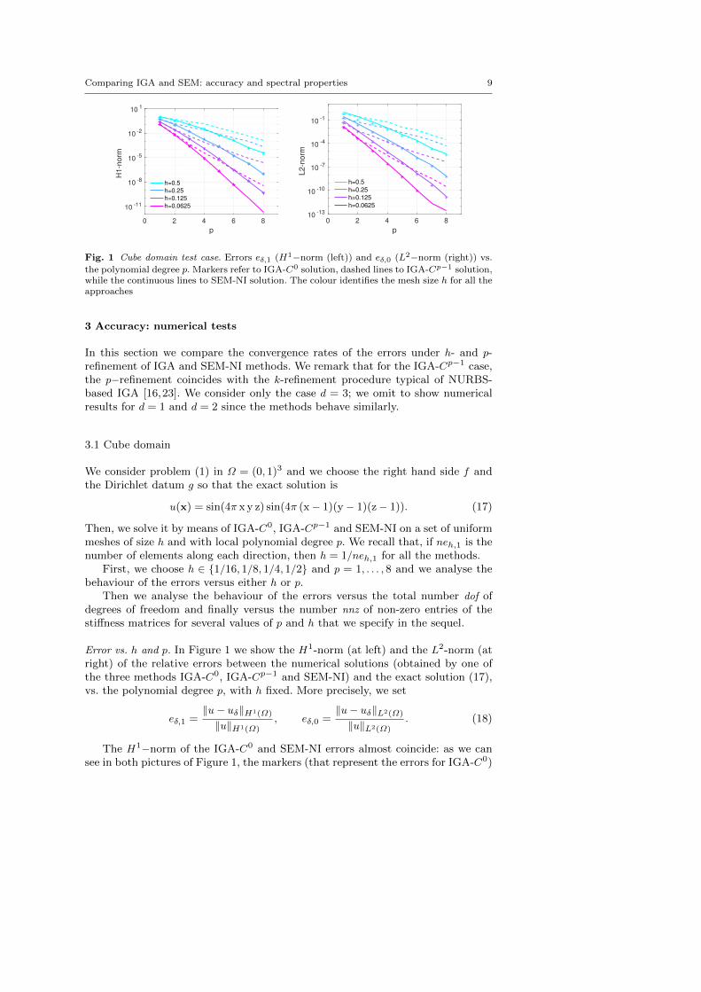
Fig. 1 Cube domain test case. Errors eδ,1 (H1−norm (left)) and eδ,0 (L2−norm (right)) vs.
the polynomial degree p. Markers refer to IGA-C0 solution, dashed lines to IGA-Cp−1 solution,while the continuous lines to SEM-NI solution. The colour identifies the mesh size h for all theapproaches
3 Accuracy: numerical tests
In this section we compare the convergence rates of the errors under h- and p-refinement of IGA and SEM-NI methods. We remark that for the IGA-Cp−1 case,the p−refinement coincides with the k-refinement procedure typical of NURBS-based IGA [16,23]. We consider only the case d = 3; we omit to show numericalresults for d = 1 and d = 2 since the methods behave similarly.
3.1 Cube domain
We consider problem (1) in Ω = (0, 1)3 and we choose the right hand side f andthe Dirichlet datum g so that the exact solution is
u(x) = sin(4π x y z) sin(4π (x− 1)(y − 1)(z− 1)). (17)
Then, we solve it by means of IGA-C0, IGA-Cp−1 and SEM-NI on a set of uniformmeshes of size h and with local polynomial degree p. We recall that, if neh,1 is thenumber of elements along each direction, then h = 1/neh,1 for all the methods.
First, we choose h ∈ 1/16, 1/8, 1/4, 1/2 and p = 1, . . . , 8 and we analyse thebehaviour of the errors versus either h or p.
Then we analyse the behaviour of the errors versus the total number dof ofdegrees of freedom and finally versus the number nnz of non-zero entries of thestiffness matrices for several values of p and h that we specify in the sequel.
Error vs. h and p. In Figure 1 we show the H1-norm (at left) and the L2-norm (atright) of the relative errors between the numerical solutions (obtained by one ofthe three methods IGA-C0, IGA-Cp−1 and SEM-NI) and the exact solution (17),vs. the polynomial degree p, with h fixed. More precisely, we set
eδ,1 =‖u− uδ‖H1(Ω)
‖u‖H1(Ω), eδ,0 =
‖u− uδ‖L2(Ω)
‖u‖L2(Ω). (18)
The H1−norm of the IGA-C0 and SEM-NI errors almost coincide: as we cansee in both pictures of Figure 1, the markers (that represent the errors for IGA-C0)
10 Paola Gervasio et al.
0.06 0.1 0.2 0.3 0.5
h
10 -11
10 -8
10 -5
10 -2
10 1
H1-n
orm
1
2
3
4
p=1
p=2
p=3
p=4
0.06 0.1 0.2 0.3 0.5
h
10 -11
10 -8
10 -5
10 -2
10 1
H1-n
orm 5
6
7
8
p=5
p=6
p=7
p=8
0.06 0.1 0.2 0.3 0.5
h
10 -13
10 -10
10 -7
10 -4
10 -1
L2
-no
rm
2
3
4
5
p=1
p=2
p=3
p=4
0.06 0.1 0.2 0.3 0.5
h
10 -13
10 -10
10 -7
10 -4
10 -1
L2
-no
rm 6
7
8 9
p=5
p=6
p=7
p=8
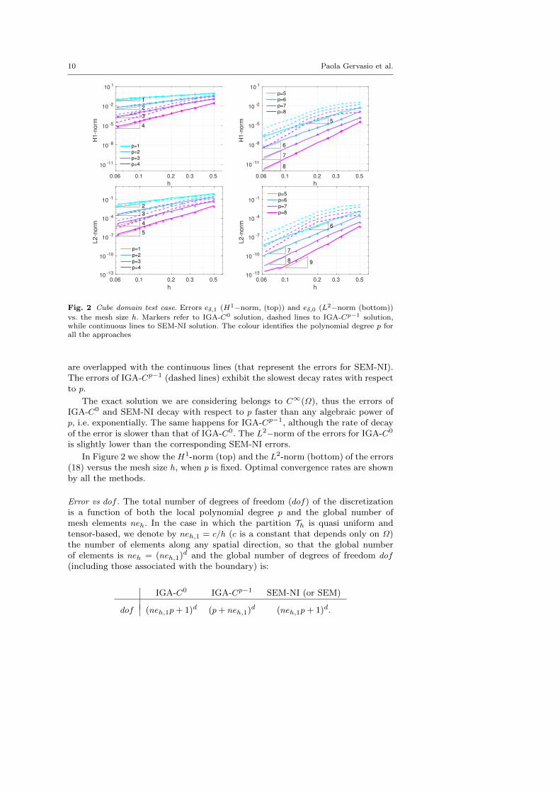
Fig. 2 Cube domain test case. Errors eδ,1 (H1−norm, (top)) and eδ,0 (L2−norm (bottom))
vs. the mesh size h. Markers refer to IGA-C0 solution, dashed lines to IGA-Cp−1 solution,while continuous lines to SEM-NI solution. The colour identifies the polynomial degree p forall the approaches
are overlapped with the continuous lines (that represent the errors for SEM-NI).The errors of IGA-Cp−1 (dashed lines) exhibit the slowest decay rates with respectto p.
The exact solution we are considering belongs to C∞(Ω), thus the errors ofIGA-C0 and SEM-NI decay with respect to p faster than any algebraic power ofp, i.e. exponentially. The same happens for IGA-Cp−1, although the rate of decayof the error is slower than that of IGA-C0. The L2−norm of the errors for IGA-C0
is slightly lower than the corresponding SEM-NI errors.
In Figure 2 we show the H1-norm (top) and the L2-norm (bottom) of the errors(18) versus the mesh size h, when p is fixed. Optimal convergence rates are shownby all the methods.
Error vs dof . The total number of degrees of freedom (dof) of the discretizationis a function of both the local polynomial degree p and the global number ofmesh elements neh. In the case in which the partition Th is quasi uniform andtensor-based, we denote by neh,1 = c/h (c is a constant that depends only on Ω)the number of elements along any spatial direction, so that the global numberof elements is neh = (neh,1)d and the global number of degrees of freedom dof
(including those associated with the boundary) is:
IGA-C0 IGA-Cp−1 SEM-NI (or SEM)
dof (neh,1p+ 1)d (p+ neh,1)d (neh,1p+ 1)d.
Comparing IGA and SEM: accuracy and spectral properties 11
101
102
103
104
105
106
dof
10-14
10-10
10-6
10-2
101
H1-n
orm
IGA-C0
IGA, 1 element
IGA-C(p-1)
SEM-NI
SEM-NI, 1 element
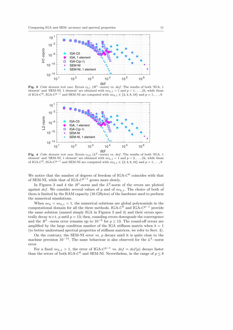
Fig. 3 Cube domain test case. Errors eδ,1 (H1−norm) vs. dof . The results of both ‘IGA, 1element’ and ‘SEM-NI, 1 element’ are obtained with neh,1 = 1 and p = 1, . . . , 24, while those
of IGA-C0, IGA-Cp−1 and SEM-NI are computed with neh,1 ∈ 2, 4, 8, 16 and p = 1, . . . , 8
101
102
103
104
105
106
dof
10-14
10-10
10-6
10-2
101
L2
-no
rm
IGA-C0
IGA, 1 element
IGA-C(p-1)
SEM-NI
SEM-NI, 1 element
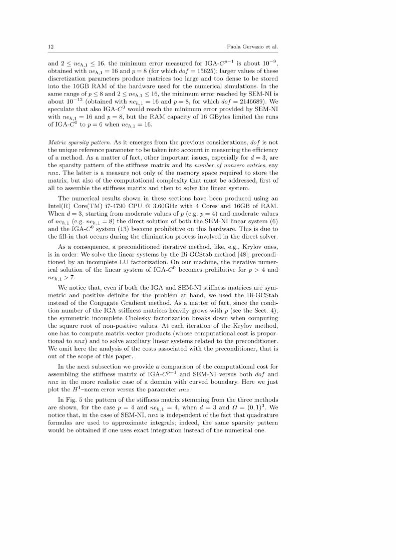
Fig. 4 Cube domain test case. Errors eδ,0 (L2−norm) vs. dof . The results of both ‘IGA, 1element’ and ‘SEM-NI, 1 element’ are obtained with neh,1 = 1 and p = 2, . . . , 24, while those
of IGA-C0, IGA-Cp−1 and SEM-NI are computed with neh,1 ∈ 2, 4, 8, 16 and p = 1, . . . , 8
We notice that the number of degrees of freedom of IGA-C0 coincides with thatof SEM-NI, while that of IGA-Cp−1 grows more slowly.
In Figures 3 and 4 the H1-norm and the L2-norm of the errors are plottedagainst dof . We consider several values of p and of neh,1. The choice of both ofthem is limited by the RAM capacity (16 GBytes) of the hardware used to performthe numerical simulations.
When neh = neh,1 = 1, the numerical solutions are global polynomials in thecomputational domain for all the three methods. IGA-C0 and IGA-Cp−1 providethe same solution (named simply IGA in Figures 3 and 4) and their errors spec-trally decay w.r.t. p until p = 13; then, rounding errors downgrade the convergenceand the H1−norm error remains up to 10−6 for p ≥ 13. The round-off errors areamplified by the large condition number of the IGA stiffness matrix when h = 1(to better understand spectral properties of stiffness matrices, we refer to Sect. 4).
On the contrary, the SEM-NI error vs. p decays until it is quite close to themachine precision 10−14. The same behaviour is also observed for the L2−normerror.
For a fixed neh,1 > 1, the error of IGA-Cp−1 vs. dof = dof(p) decays fasterthan the errors of both IGA-C0 and SEM-NI. Nevertheless, in the range of p ≤ 8
12 Paola Gervasio et al.
and 2 ≤ neh,1 ≤ 16, the minimum error measured for IGA-Cp−1 is about 10−9,obtained with neh,1 = 16 and p = 8 (for which dof = 15625); larger values of thesediscretization parameters produce matrices too large and too dense to be storedinto the 16GB RAM of the hardware used for the numerical simulations. In thesame range of p ≤ 8 and 2 ≤ neh,1 ≤ 16, the minimum error reached by SEM-NI isabout 10−12 (obtained with neh,1 = 16 and p = 8, for which dof = 2146689). Wespeculate that also IGA-C0 would reach the minimum error provided by SEM-NIwith neh,1 = 16 and p = 8, but the RAM capacity of 16 GBytes limited the runsof IGA-C0 to p = 6 when neh,1 = 16.
Matrix sparsity pattern. As it emerges from the previous considerations, dof is notthe unique reference parameter to be taken into account in measuring the efficiencyof a method. As a matter of fact, other important issues, especially for d = 3, arethe sparsity pattern of the stiffness matrix and its number of nonzero entries, saynnz. The latter is a measure not only of the memory space required to store thematrix, but also of the computational complexity that must be addressed, first ofall to assemble the stiffness matrix and then to solve the linear system.
The numerical results shown in these sections have been produced using anIntel(R) Core(TM) i7-4790 CPU @ 3.60GHz with 4 Cores and 16GB of RAM.When d = 3, starting from moderate values of p (e.g. p = 4) and moderate valuesof neh,1 (e.g. neh,1 = 8) the direct solution of both the SEM-NI linear system (6)and the IGA-C0 system (13) become prohibitive on this hardware. This is due tothe fill-in that occurs during the elimination process involved in the direct solver.
As a consequence, a preconditioned iterative method, like, e.g., Krylov ones,is in order. We solve the linear systems by the Bi-GCStab method [48], precondi-tioned by an incomplete LU factorization. On our machine, the iterative numer-ical solution of the linear system of IGA-C0 becomes prohibitive for p > 4 andneh,1 > 7.
We notice that, even if both the IGA and SEM-NI stiffness matrices are sym-metric and positive definite for the problem at hand, we used the Bi-GCStabinstead of the Conjugate Gradient method. As a matter of fact, since the condi-tion number of the IGA stiffness matrices heavily grows with p (see the Sect. 4),the symmetric incomplete Cholesky factorization breaks down when computingthe square root of non-positive values. At each iteration of the Krylov method,one has to compute matrix-vector products (whose computational cost is propor-tional to nnz) and to solve auxiliary linear systems related to the preconditioner.We omit here the analysis of the costs associated with the preconditioner, that isout of the scope of this paper.
In the next subsection we provide a comparison of the computational cost forassembling the stiffness matrix of IGA-Cp−1 and SEM-NI versus both dof andnnz in the more realistic case of a domain with curved boundary. Here we justplot the H1–norm error versus the parameter nnz.
In Fig. 5 the pattern of the stiffness matrix stemming from the three methodsare shown, for the case p = 4 and neh,1 = 4, when d = 3 and Ω = (0, 1)3. Wenotice that, in the case of SEM-NI, nnz is independent of the fact that quadratureformulas are used to approximate integrals; indeed, the same sparsity patternwould be obtained if one uses exact integration instead of the numerical one.
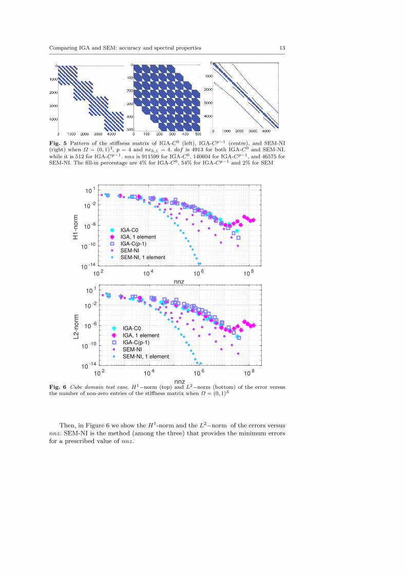
Comparing IGA and SEM: accuracy and spectral properties 13
Fig. 5 Pattern of the stiffness matrix of IGA-C0 (left), IGA-Cp−1 (centre), and SEM-NI(right) when Ω = (0, 1)3, p = 4 and neh,1 = 4. dof is 4913 for both IGA-C0 and SEM-NI,
while it is 512 for IGA-Cp−1. nnz is 911599 for IGA-C0, 140604 for IGA-Cp−1, and 46575 forSEM-NI. The fill-in percentage are 4% for IGA-C0, 54% for IGA-Cp−1 and 2% for SEM
102
104
106
108
nnz
10-14
10-10
10-6
10-2
101
H1
-no
rm
IGA-C0
IGA, 1 element
IGA-C(p-1)
SEM-NI
SEM-NI, 1 element
102
104
106
108
nnz
10-14
10-10
10-6
10-2
101
L2-n
orm
IGA-C0
IGA, 1 element
IGA-C(p-1)
SEM-NI
SEM-NI, 1 element
Fig. 6 Cube domain test case. H1−norm (top) and L2−norm (bottom) of the error versusthe number of non-zero entries of the stiffness matrix when Ω = (0, 1)3
Then, in Figure 6 we show the H1-norm and the L2−norm of the errors versusnnz. SEM-NI is the method (among the three) that provides the minimum errorsfor a prescribed value of nnz.
14 Paola Gervasio et al.
00.5x110.8
y0.60.40.20
0.9
0.8
0.7
0.6
0.5
0.4
0.3
0.2
0.1
0
1
z
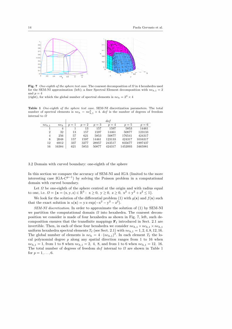
Fig. 7 One-eighth of the sphere test case. The coarsest decomposition ofΩ in 4 hexahedra usedfor the SEM-NI approximation (left); a finer Spectral Element decomposition with neh,1 = 2and p = 4(right), for which the global number of spectral elements is neh = 23 × 4
Table 1 One-eighth of the sphere test case. SEM-NI discretization parameters. The totalnumber of spectral elements is neh = ne3h,1 × 4. dof is the number of degrees of freedom
internal to Ω
dofneh,1 neh p = 1 p = 2 p = 3 p = 4 p = 5 p = 6
1 4 1 13 157 1597 5853 144612 32 13 157 1597 14461 50877 1231334 256 57 621 5853 50877 176541 4243178 2048 157 1597 14461 123133 424317 1016317
12 6912 337 3277 28957 243517 835677 199743716 16384 621 5853 50877 424317 1452093 3465981
3.2 Domain with curved boundary: one-eighth of the sphere
In this section we compare the accuracy of SEM-NI and IGA (limited to the moreinteresting case IGA-Cp−1) by solving the Poisson problem in a computationaldomain with curved boundary.
Let Ω be one-eighth of the sphere centred at the origin and with radius equalto one, i.e. Ω = x = (x,y, z) ∈ R3 : x ≥ 0, y ≥ 0, z ≥ 0, x2 + y2 + z2 ≤ 1.
We look for the solution of the differential problem (1) with g(x) and f(x) suchthat the exact solution is u(x) = y z exp(−x2 − y2 − z2).
SEM-NI discretization. In order to approximate the solution of (1) by SEM-NIwe partition the computational domain Ω into hexahedra. The coarsest decom-position we consider is made of four hexahedra as shown in Fig. 7, left, such de-composition ensures that the transfinite mappings F` introduced in Sect. 2.1 areinvertible. Then, in each of these four hexahedra we consider neh,1 × neh,1 × neh,1uniform hexahedra spectral elements T` (see Sect. 2.1) with neh,1 = 1, 2, 4, 8, 12, 16.The global number of elements is neh = 4 · (neh,1)3. In each element T` the lo-cal polynomial degree p along any spatial direction ranges from 1 to 16 whenneh,1 = 1, from 1 to 8 when neh,1 = 2, 4, 8, and from 1 to 6 when neh,1 = 12, 16.The total number of degrees of freedom dof internal to Ω are shown in Table 1for p = 1, . . . , 6.
Comparing IGA and SEM: accuracy and spectral properties 15
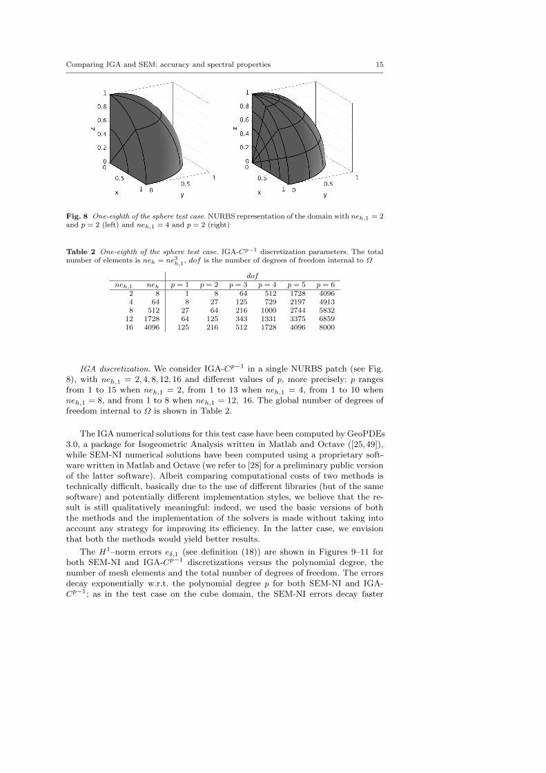
Fig. 8 One-eighth of the sphere test case. NURBS representation of the domain with neh,1 = 2and p = 2 (left) and neh,1 = 4 and p = 2 (right)
Table 2 One-eighth of the sphere test case. IGA-Cp−1 discretization parameters. The totalnumber of elements is neh = ne3h,1, dof is the number of degrees of freedom internal to Ω
dofneh,1 neh p = 1 p = 2 p = 3 p = 4 p = 5 p = 6
2 8 1 8 64 512 1728 40964 64 8 27 125 729 2197 49138 512 27 64 216 1000 2744 5832
12 1728 64 125 343 1331 3375 685916 4096 125 216 512 1728 4096 8000
IGA discretization. We consider IGA-Cp−1 in a single NURBS patch (see Fig.8), with neh,1 = 2, 4, 8, 12, 16 and different values of p, more precisely: p rangesfrom 1 to 15 when neh,1 = 2, from 1 to 13 when neh,1 = 4, from 1 to 10 whenneh,1 = 8, and from 1 to 8 when neh,1 = 12, 16. The global number of degrees offreedom internal to Ω is shown in Table 2.
The IGA numerical solutions for this test case have been computed by GeoPDEs3.0, a package for Isogeometric Analysis written in Matlab and Octave ([25,49]),while SEM-NI numerical solutions have been computed using a proprietary soft-ware written in Matlab and Octave (we refer to [28] for a preliminary public versionof the latter software). Albeit comparing computational costs of two methods istechnically difficult, basically due to the use of different libraries (but of the samesoftware) and potentially different implementation styles, we believe that the re-sult is still qualitatively meaningful: indeed, we used the basic versions of boththe methods and the implementation of the solvers is made without taking intoaccount any strategy for improving its efficiency. In the latter case, we envisionthat both the methods would yield better results.
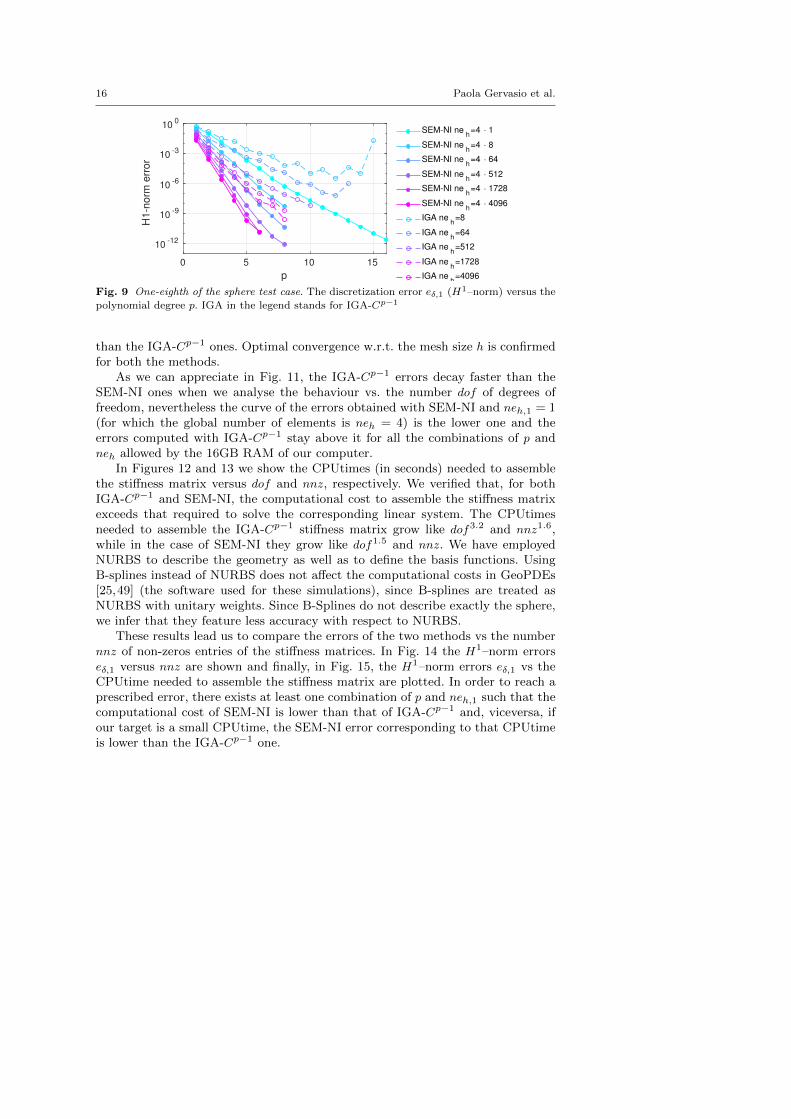
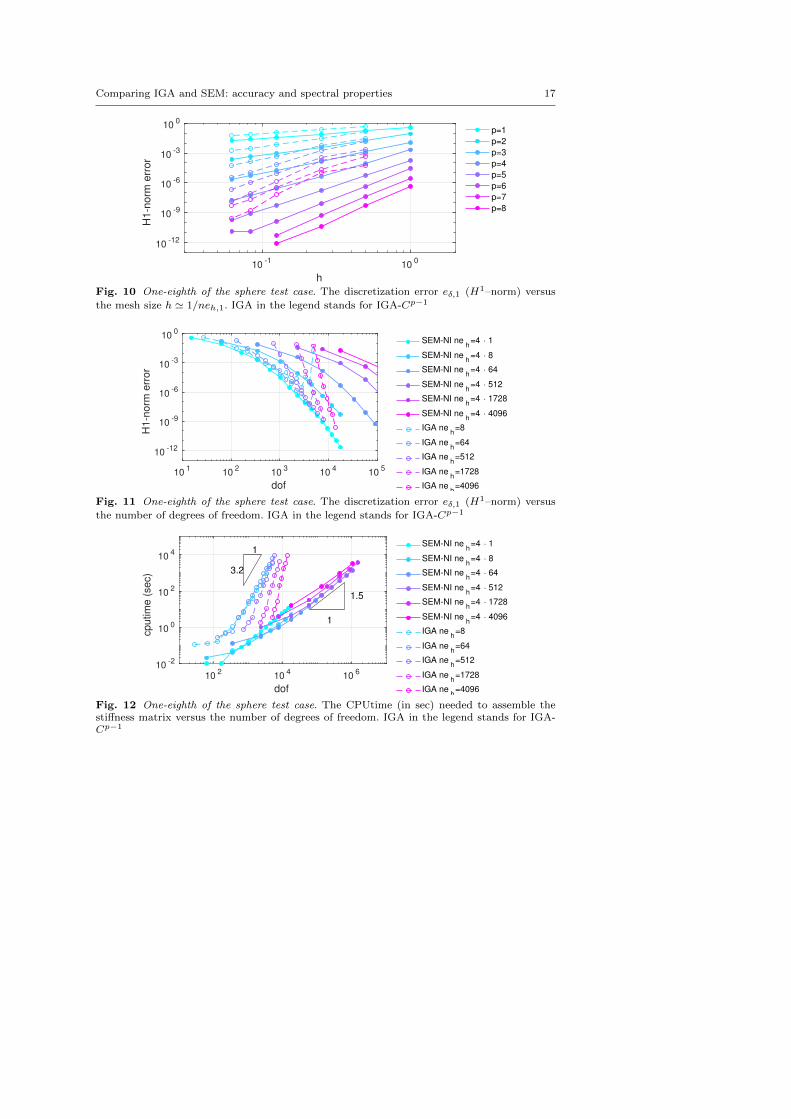
The H1–norm errors eδ,1 (see definition (18)) are shown in Figures 9–11 forboth SEM-NI and IGA-Cp−1 discretizations versus the polynomial degree, thenumber of mesh elements and the total number of degrees of freedom. The errorsdecay exponentially w.r.t. the polynomial degree p for both SEM-NI and IGA-Cp−1; as in the test case on the cube domain, the SEM-NI errors decay faster
16 Paola Gervasio et al.
0 5 10 15
p
10-12
10-9
10-6
10-3
100
H1
-no
rm e
rro
r
SEM-NI neh=4 1
SEM-NI neh=4 8
SEM-NI neh=4 64
SEM-NI neh=4 512
SEM-NI neh=4 1728
SEM-NI neh=4 4096
IGA neh=8
IGA neh=64
IGA neh=512
IGA neh=1728
IGA neh=4096
Fig. 9 One-eighth of the sphere test case. The discretization error eδ,1 (H1–norm) versus the
polynomial degree p. IGA in the legend stands for IGA-Cp−1
than the IGA-Cp−1 ones. Optimal convergence w.r.t. the mesh size h is confirmedfor both the methods.
As we can appreciate in Fig. 11, the IGA-Cp−1 errors decay faster than theSEM-NI ones when we analyse the behaviour vs. the number dof of degrees offreedom, nevertheless the curve of the errors obtained with SEM-NI and neh,1 = 1(for which the global number of elements is neh = 4) is the lower one and theerrors computed with IGA-Cp−1 stay above it for all the combinations of p andneh allowed by the 16GB RAM of our computer.
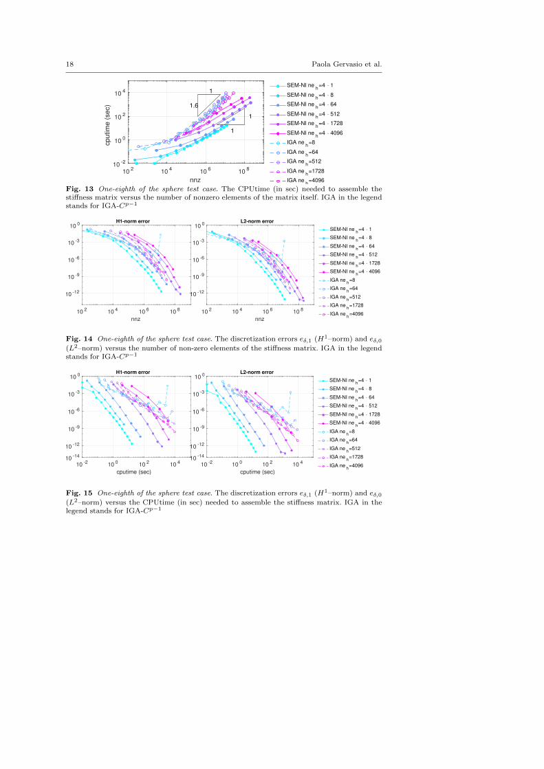
In Figures 12 and 13 we show the CPUtimes (in seconds) needed to assemblethe stiffness matrix versus dof and nnz, respectively. We verified that, for bothIGA-Cp−1 and SEM-NI, the computational cost to assemble the stiffness matrixexceeds that required to solve the corresponding linear system. The CPUtimesneeded to assemble the IGA-Cp−1 stiffness matrix grow like dof3.2 and nnz1.6,while in the case of SEM-NI they grow like dof1.5 and nnz. We have employedNURBS to describe the geometry as well as to define the basis functions. UsingB-splines instead of NURBS does not affect the computational costs in GeoPDEs[25,49] (the software used for these simulations), since B-splines are treated asNURBS with unitary weights. Since B-Splines do not describe exactly the sphere,we infer that they feature less accuracy with respect to NURBS.
These results lead us to compare the errors of the two methods vs the numbernnz of non-zeros entries of the stiffness matrices. In Fig. 14 the H1–norm errorseδ,1 versus nnz are shown and finally, in Fig. 15, the H1–norm errors eδ,1 vs theCPUtime needed to assemble the stiffness matrix are plotted. In order to reach aprescribed error, there exists at least one combination of p and neh,1 such that thecomputational cost of SEM-NI is lower than that of IGA-Cp−1 and, viceversa, ifour target is a small CPUtime, the SEM-NI error corresponding to that CPUtimeis lower than the IGA-Cp−1 one.
Comparing IGA and SEM: accuracy and spectral properties 17
10-1
100
h
10-12
10-9
10-6
10-3
100
H1
-no
rm e
rro
r
p=1
p=2
p=3
p=4
p=5
p=6
p=7
p=8
Fig. 10 One-eighth of the sphere test case. The discretization error eδ,1 (H1–norm) versus
the mesh size h ' 1/neh,1. IGA in the legend stands for IGA-Cp−1
101
102
103
104
105
dof
10-12
10-9
10-6
10-3
100
H1
-no
rm e
rro
r
SEM-NI neh=4 1
SEM-NI neh=4 8
SEM-NI neh=4 64
SEM-NI neh=4 512
SEM-NI neh=4 1728
SEM-NI neh=4 4096
IGA neh=8
IGA neh=64
IGA neh=512
IGA neh=1728
IGA neh=4096
Fig. 11 One-eighth of the sphere test case. The discretization error eδ,1 (H1–norm) versus
the number of degrees of freedom. IGA in the legend stands for IGA-Cp−1
102
104
106
dof
10-2
100
102
104
cputim
e (
sec)
1.5
1
3.2
1SEM-NI ne
h=4 1
SEM-NI neh=4 8
SEM-NI neh=4 64
SEM-NI neh=4 512
SEM-NI neh=4 1728
SEM-NI neh=4 4096
IGA neh=8
IGA neh=64
IGA neh=512
IGA neh=1728
IGA neh=4096
Fig. 12 One-eighth of the sphere test case. The CPUtime (in sec) needed to assemble thestiffness matrix versus the number of degrees of freedom. IGA in the legend stands for IGA-Cp−1
18 Paola Gervasio et al.
102
104
106
108
nnz
10-2
100
102
104
cputim
e (
sec)
1
1
1.6
1SEM-NI ne
h=4 1
SEM-NI neh=4 8
SEM-NI neh=4 64
SEM-NI neh=4 512
SEM-NI neh=4 1728
SEM-NI neh=4 4096
IGA neh=8
IGA neh=64
IGA neh=512
IGA neh=1728
IGA neh=4096
Fig. 13 One-eighth of the sphere test case. The CPUtime (in sec) needed to assemble thestiffness matrix versus the number of nonzero elements of the matrix itself. IGA in the legendstands for IGA-Cp−1
102
104
106
108
nnz
10-12
10-9
10-6
10-3
100
H1-norm error
102
104
106
108
nnz
10-12
10-9
10-6
10-3
100
L2-norm error
SEM-NI neh=4 1
SEM-NI neh=4 8
SEM-NI neh=4 64
SEM-NI neh=4 512
SEM-NI neh=4 1728
SEM-NI neh=4 4096
IGA neh=8
IGA neh=64
IGA neh=512
IGA neh=1728
IGA neh=4096
Fig. 14 One-eighth of the sphere test case. The discretization errors eδ,1 (H1–norm) and eδ,0(L2–norm) versus the number of non-zero elements of the stiffness matrix. IGA in the legendstands for IGA-Cp−1
10 -2 10 0 10 2 10 4
cputime (sec)
10 -14
10 -12
10 -9
10 -6
10 -3
10 0H1-norm error
10 -2 10 0 10 2 10 4
cputime (sec)
10 -14
10 -12
10 -9
10 -6
10 -3
10 0L2-norm error
SEM-NI neh=4 1
SEM-NI neh=4 8
SEM-NI neh=4 64
SEM-NI neh=4 512
SEM-NI neh=4 1728
SEM-NI neh=4 4096
IGA neh=8
IGA neh=64
IGA neh=512
IGA neh=1728
IGA neh=4096
Fig. 15 One-eighth of the sphere test case. The discretization errors eδ,1 (H1–norm) and eδ,0(L2–norm) versus the CPUtime (in sec) needed to assemble the stiffness matrix. IGA in thelegend stands for IGA-Cp−1
Comparing IGA and SEM: accuracy and spectral properties 19
4 Spectral properties: eigenvalues and condition number
In this section we summarise the main results concerning the spectral propertiesof SEM-NI and IGA arrays. Because of their importance for the convergence rateof iterative methods for the solution of the linear system, as well as for the prop-agation of rounding errors in solving the linear system itself (see, e.g., Figs. 3, 6,and 9), we specifically highlight the behaviour of the extreme eigenvalues (and thecorresponding spectral condition number) of mass matrices and stiffness matrices.
For any matrix A which is symmetric positive definite (or similar to a sym-metric positive definite matrix), let λmin(A) and λmax(A) denote its minimumand maximum (real) eigenvalues, respectively. The spectral condition number of Ais defined as
K(A) =λmax(A)
λmin(A). (19)
The extreme eigenvalues of the SEM-NI mass and stiffness matrices (5) (thelatter reduced to the rows and columns associated with the nodes internal toΩ = (0, 1)d) behave as follows ([9,38,13,14,12]):
λmin(MSEM ) ∼ hdp−2d (20)
λmax(MSEM ) ∼ hdp−d (21)
λmin(KSEM ) ∼ hdp−d (22)
λmax(KSEM ) ∼ hd−2p3−d (23)
λmin((MSEM )−1KSEM ) ∼ c (24)
λmin((MSEM )−1KSEM ) ∼ h−2p4. (25)
The corresponding spectral condition numbers for d = 1, 2, 3 are:
K(MSEM ) ∼ pd (26)
K(KSEM ) ∼ p3h−2 (27)
K((MSEM )−1KSEM ) ∼ p4h−2; (28)
these are reported in Table 3. In the whole section the symbol ∼ means “up to a
constant independent of both p and h”.The eigenvalues and the condition number of IGA matrices have been studied
in [26,27]. In [26] it is proved for d = 2 that, independently of the k-regularity ofthe B-spline basis functions, it holds:
λmin(Mk) ∼ c(p)h2, λmin(Mk) ≥ c(h)p−416−p
λmax(Mk) ∼ c(p)h2, λmax(Mk) ∼ c(h)p−2,
K(Mk) ≤ cp216p, with c independent of h and p,
λmin(Kk) ∼ c(p)h2,λmax(Kk) ∼ c, with c independent of h and p,
K(Kk) ≤ c(h)p816p,
(29)
where Mk and Kk are the mass matrix and the stiffness matrix of IGA approxi-mation for a generic k = 0, . . . , p− 1. In [27] it is proved for d = 1, p ≥ 1 and n ≥ 2(where n is the number of elements, so that h ∼ 1/n) that
λmin(Mp−1) ≥ c(p)h, λmin(Kp−1) ≥ π2c(p)h. (30)
20 Paola Gervasio et al.
Other estimates about the clustering of the eigenvalues of the matrix correspondingto the IGA approximation of the advection-diffusion-reaction operator for d = 1are proved in [27].
We have numerically computed the extreme eigenvalues of the mass and stiff-ness matrices for both IGA-C0 and IGA-Cp−1 using the function eigs of Matlabfor different values of h and p. Starting from these values we have estimated theanalytic behaviour of the extreme eigenvalues (and then the spectral conditionnumber) of the IGA matrices w.r.t. both h and p.
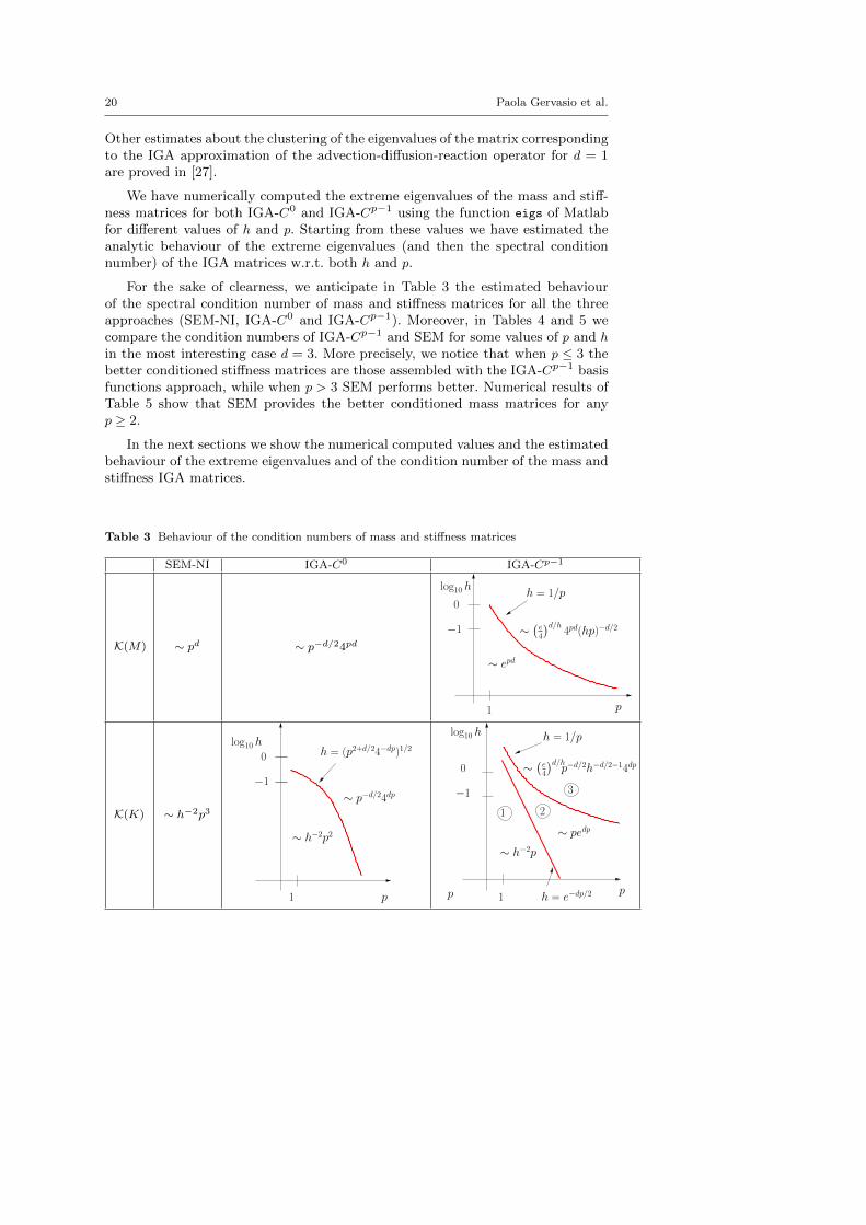
For the sake of clearness, we anticipate in Table 3 the estimated behaviourof the spectral condition number of mass and stiffness matrices for all the threeapproaches (SEM-NI, IGA-C0 and IGA-Cp−1). Moreover, in Tables 4 and 5 wecompare the condition numbers of IGA-Cp−1 and SEM for some values of p and h
in the most interesting case d = 3. More precisely, we notice that when p ≤ 3 thebetter conditioned stiffness matrices are those assembled with the IGA-Cp−1 basisfunctions approach, while when p > 3 SEM performs better. Numerical results ofTable 5 show that SEM provides the better conditioned mass matrices for anyp ≥ 2.
In the next sections we show the numerical computed values and the estimatedbehaviour of the extreme eigenvalues and of the condition number of the mass andstiffness IGA matrices.
Table 3 Behaviour of the condition numbers of mass and stiffness matrices
SEM-NI IGA-C0 IGA-Cp−1
K(M) ∼ pd ∼ p−d/24pd
0
−1
log10 h h = 1/p
∼(e4
)d/h4pd(hp)−d/2
∼ epd
1 p
K(K) ∼ h−2p3
1 p
∼ h−2p2
0
−1
log10 h
p
h = (p2+d/24−dp)1/2
∼ p−d/24dp
∼ h−2p
log10 h
h = e−dp/2
∼ pedp
p1
−1
0 ∼(e4
)d/hp−d/2h−d/2−14dp
h = 1/p
1 2
3
Comparing IGA and SEM: accuracy and spectral properties 21
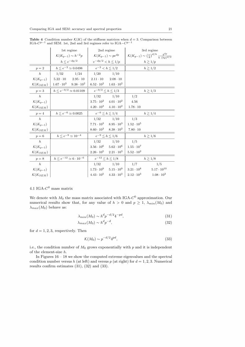
Table 4 Condition number K(K) of the stiffness matrices when d = 3. Comparison betweenIGA-Cp−1 and SEM. 1st, 2nd and 3rd regimes refer to IGA−Cp−1
1st regime 2nd regime 3rd regime
K(Kp−1) ∼ h−2p K(Kp−1) ∼ pedp K(Kp−1) ∼(e4
)d/h 4dp
h (hp)d/2
h . e−dp/2 e−dp/2 < h . 1/p h & 1/p
p = 2 h . e−3 ' 0.0498 e−3 < h . 1/2 h & 1/2
h 1/32 1/24 1/20 1/10
K(Kp−1) 5.22 · 10 2.95 · 10 2.11 · 10 2.08 · 10
K(KSEM ) 1.67 · 103 9.38 · 102 6.52 · 102 1.63 · 102
p = 3 h . e−9/2 ' 0.01109 e−9/2 . h . 1/3 h & 1/3
h 1/32 1/10 1/2
K(Kp−1) 3.75 · 102 4.01 · 102 4.56
K(KSEM ) 4.20 · 103 4.10 · 102 1.78 · 10
p = 4 h . e−6 ' 0.0025 e−6 . h . 1/4 h & 1/4
h 1/32 1/10 1/3
K(Kp−1) 7.71 · 103 8.95 · 103 1.52 · 105
K(KSEM ) 8.60 · 103 8.38 · 102 7.80 · 10
p = 6 h . e−9 ' 10−4 e−9 . h . 1/6 h & 1/6
h 1/32 1/10 1/5
K(Kp−1) 3.56 · 106 5.62 · 106 1.55 · 107
K(KSEM ) 2.26 · 105 2.21 · 103 5.52 · 102
p = 8 h . e−12 ' 6 · 10−6 e−12 . h . 1/8 h & 1/8
h 1/32 1/10 1/7 1/5
K(Kp−1) 1.73 · 109 5.15 · 109 3.21 · 108 5.17 · 1010
K(KSEM ) 4.43 · 105 4.33 · 103 2.12 · 103 1.08 · 103
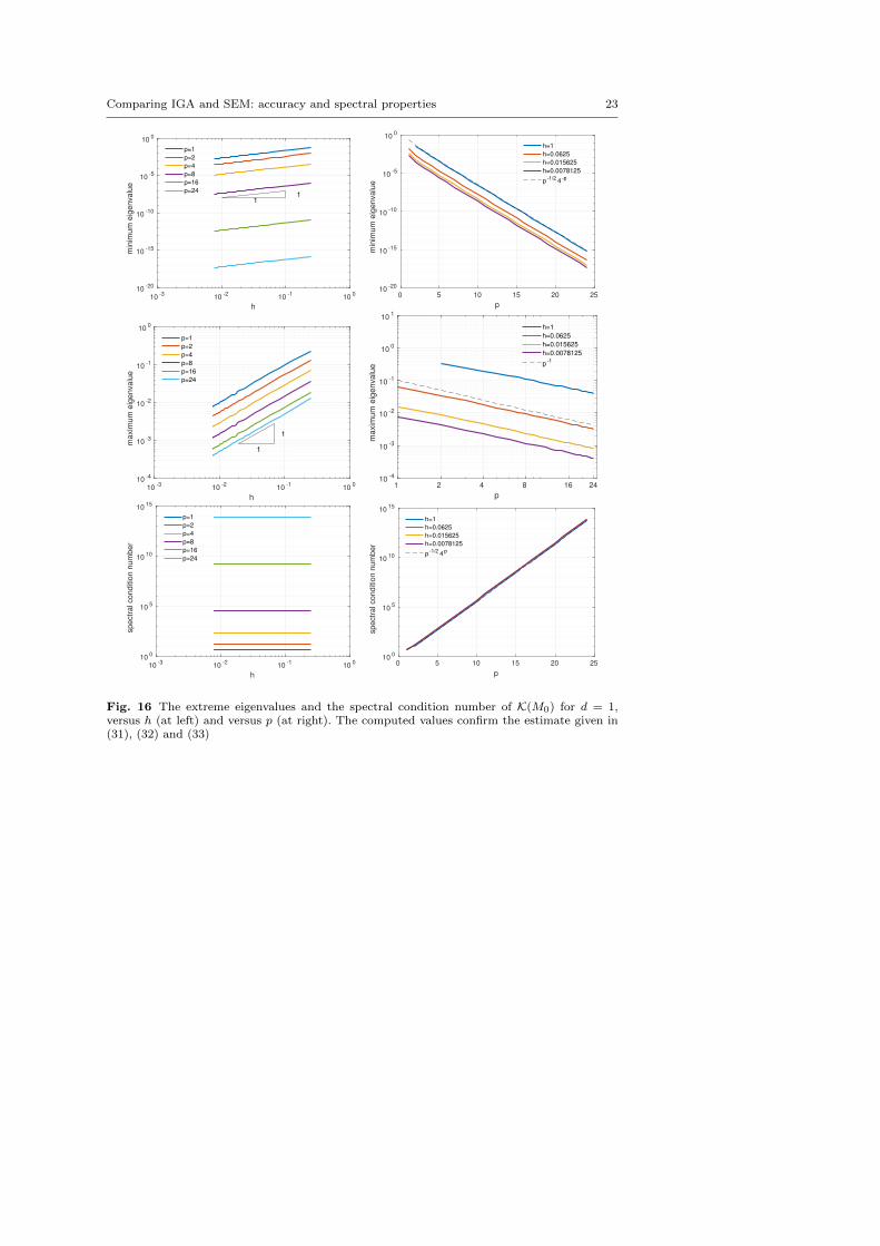
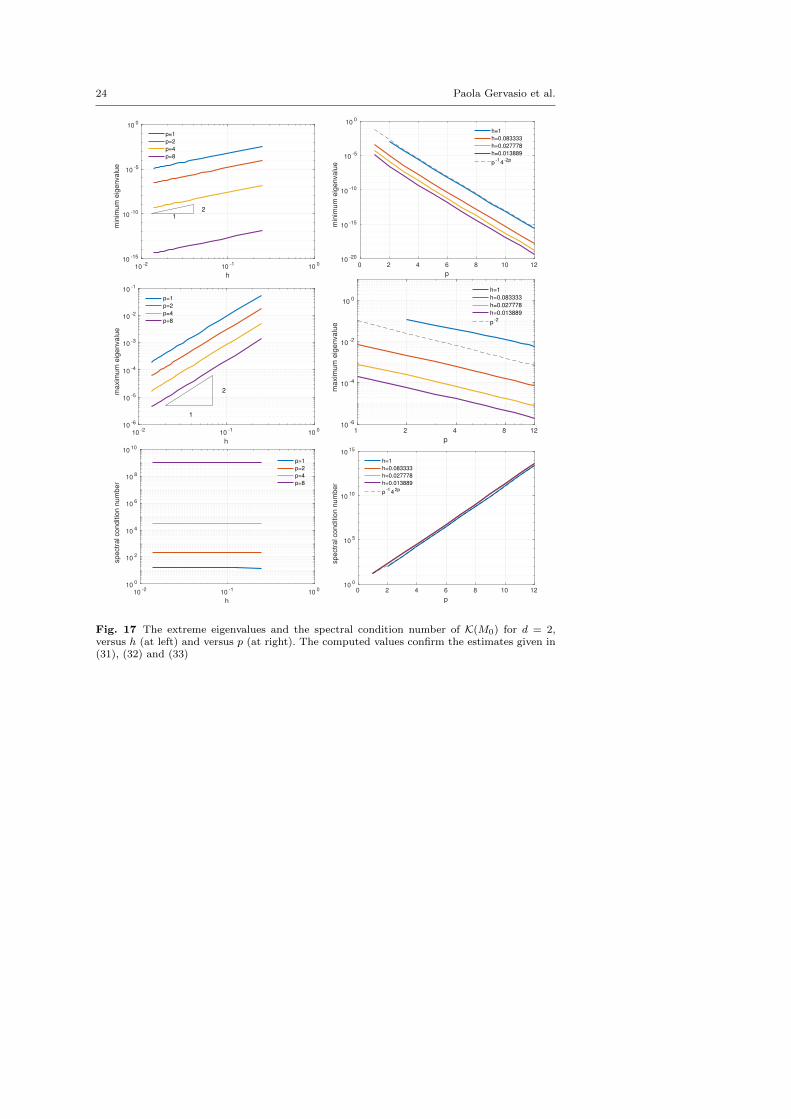
4.1 IGA-C0 mass matrix
We denote with M0 the mass matrix associated with IGA-C0 approximation. Ournumerical results show that, for any value of h > 0 and p ≥ 1, λmin(M0) andλmax(M0) behave as:
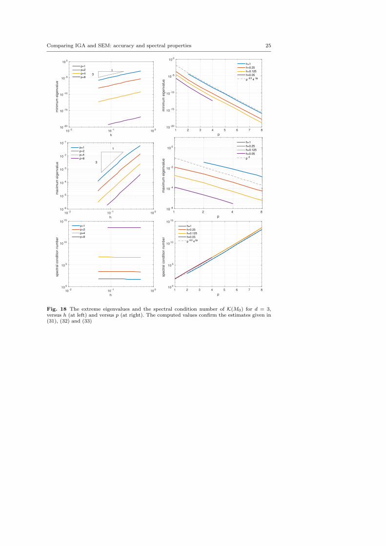
λmin(M0) ∼ hdp−d/24−pd, (31)
λmax(M0) ∼ hdp−d, (32)
for d = 1, 2, 3, respectively. Then
K(M0) ∼ p−d/24pd, (33)
i.e., the condition number of M0 grows exponentially with p and it is independentof the element-size h.
In Figures 16 – 18 we show the computed extreme eigenvalues and the spectralcondition number versus h (at left) and versus p (at right) for d = 1, 2, 3. Numericalresults confirm estimates (31), (32) and (33).
22 Paola Gervasio et al.
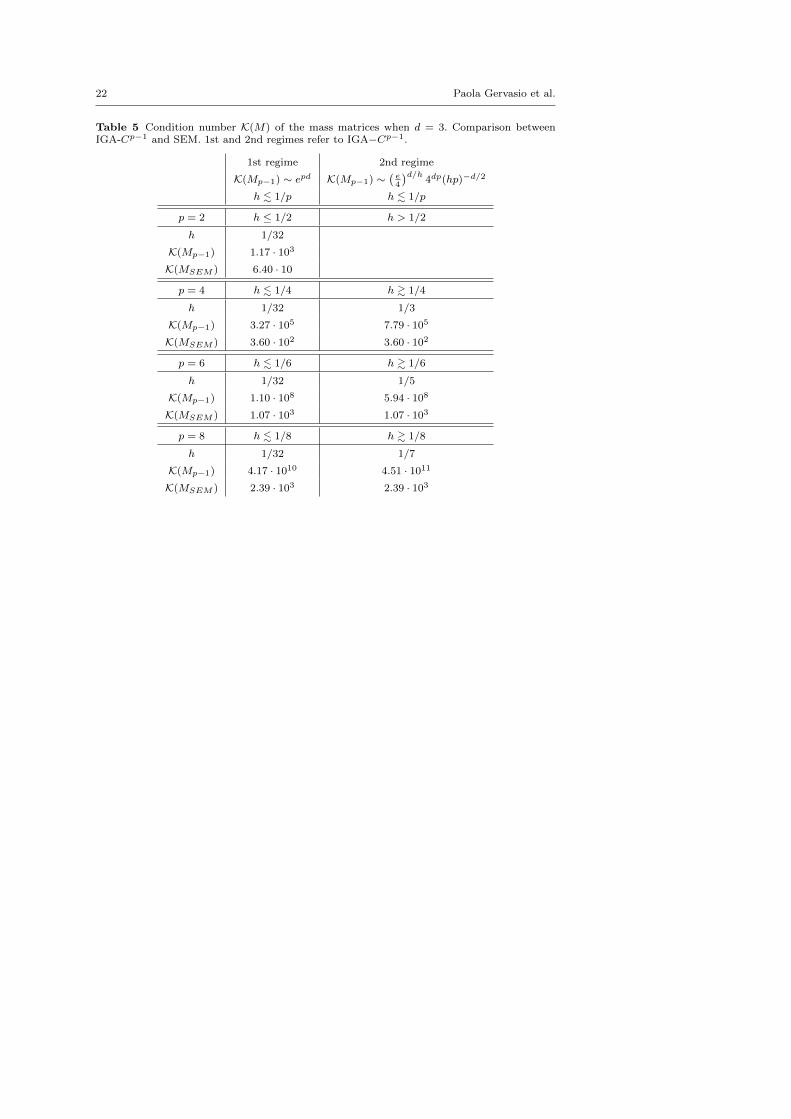
Table 5 Condition number K(M) of the mass matrices when d = 3. Comparison betweenIGA-Cp−1 and SEM. 1st and 2nd regimes refer to IGA−Cp−1.
1st regime 2nd regime
K(Mp−1) ∼ epd K(Mp−1) ∼(e4
)d/h4dp(hp)−d/2
h . 1/p h . 1/p
p = 2 h ≤ 1/2 h > 1/2
h 1/32
K(Mp−1) 1.17 · 103
K(MSEM ) 6.40 · 10
p = 4 h . 1/4 h & 1/4
h 1/32 1/3
K(Mp−1) 3.27 · 105 7.79 · 105
K(MSEM ) 3.60 · 102 3.60 · 102
p = 6 h . 1/6 h & 1/6
h 1/32 1/5
K(Mp−1) 1.10 · 108 5.94 · 108
K(MSEM ) 1.07 · 103 1.07 · 103
p = 8 h . 1/8 h & 1/8
h 1/32 1/7
K(Mp−1) 4.17 · 1010 4.51 · 1011
K(MSEM ) 2.39 · 103 2.39 · 103
Comparing IGA and SEM: accuracy and spectral properties 23
10-3
10-2
10-1
100
h
10-20
10-15
10-10
10-5
100
min
imum
eig
envalu
e
11
p=1
p=2
p=4
p=8
p=16
p=24
0 5 10 15 20 25
p
10-20
10-15
10-10
10-5
100
min
imum
eig
envalu
e
h=1
h=0.0625
h=0.015625
h=0.0078125
p-1/2
4-p
10-3
10-2
10-1
100
h
10-4
10-3
10-2
10-1
100
ma
xim
um
eig
en
va
lue
1
1
p=1
p=2
p=4
p=8
p=16
p=24
1 2 4 8 16 24
p
10-4
10-3
10-2
10-1
100
101
maxim
um
eig
envalu
e
h=1
h=0.0625
h=0.015625
h=0.0078125
p-1
10-3
10-2
10-1
100
h
100
105
1010
1015
sp
ectr
al co
nd
itio
n n
um
be
r
p=1
p=2
p=4
p=8
p=16
p=24
0 5 10 15 20 25
p
100
105
1010
1015
spectr
al conditio
n n
um
ber
h=1
h=0.0625
h=0.015625
h=0.0078125
p-1/2
4p
Fig. 16 The extreme eigenvalues and the spectral condition number of K(M0) for d = 1,versus h (at left) and versus p (at right). The computed values confirm the estimate given in(31), (32) and (33)
24 Paola Gervasio et al.
10-2
10-1
100
h
10-15
10-10
10-5
100
min
imum
eig
envalu
e
21
p=1
p=2
p=4
p=8
0 2 4 6 8 10 12
p
10-20
10-15
10-10
10-5
100
min
imum
eig
envalu
e
h=1
h=0.083333
h=0.027778
h=0.013889
p-1
4-2p
10-2
10-1
100
h
10-6
10-5
10-4
10-3
10-2
10-1
ma
xim
um
eig
en
va
lue
2
1
p=1
p=2
p=4
p=8
1 2 4 8 12
p
10-6
10-4
10-2
100
maxim
um
eig
envalu
e
h=1
h=0.083333
h=0.027778
h=0.013889
p-2
10-2
10-1
100
h
100
102
104
106
108
1010
sp
ectr
al co
nd
itio
n n
um
be
r
p=1
p=2
p=4
p=8
0 2 4 6 8 10 12
p
100
105
1010
1015
spectr
al conditio
n n
um
ber
h=1
h=0.083333
h=0.027778
h=0.013889
p-1
42p
Fig. 17 The extreme eigenvalues and the spectral condition number of K(M0) for d = 2,versus h (at left) and versus p (at right). The computed values confirm the estimates given in(31), (32) and (33)
Comparing IGA and SEM: accuracy and spectral properties 25
10-2
10-1
100
h
10-20
10-15
10-10
10-5
100
min
imum
eig
envalu
e
3
1
p=1
p=2
p=4
p=8
1 2 3 4 5 6 7 8
p
10-20
10-15
10-10
10-5
100
min
imum
eig
envalu
e
h=1
h=0.25
h=0.125
h=0.05
p-3/2
4-3p
10-2
10-1
100
h
10-6
10-5
10-4
10-3
10-2
10-1
ma
xim
um
eig
en
va
lue 3
1p=1
p=2
p=4
p=8
1 2 4 8
p
10-6
10-4
10-2
100
maxim
um
eig
envalu
e
h=1
h=0.25
h=0.125
h=0.05
p-3
10-2
10-1
100
h
100
105
1010
1015
sp
ectr
al co
nd
itio
n n
um
be
r
p=1
p=2
p=4
p=8
1 2 3 4 5 6 7 8
p
100
105
1010
1015
spectr
al conditio
n n
um
ber
h=1
h=0.25
h=0.125
h=0.05
p-3/2
43p
Fig. 18 The extreme eigenvalues and the spectral condition number of K(M0) for d = 3,versus h (at left) and versus p (at right). The computed values confirm the estimates given in(31), (32) and (33)
26 Paola Gervasio et al.
4.2 IGA-C0 stiffness matrix
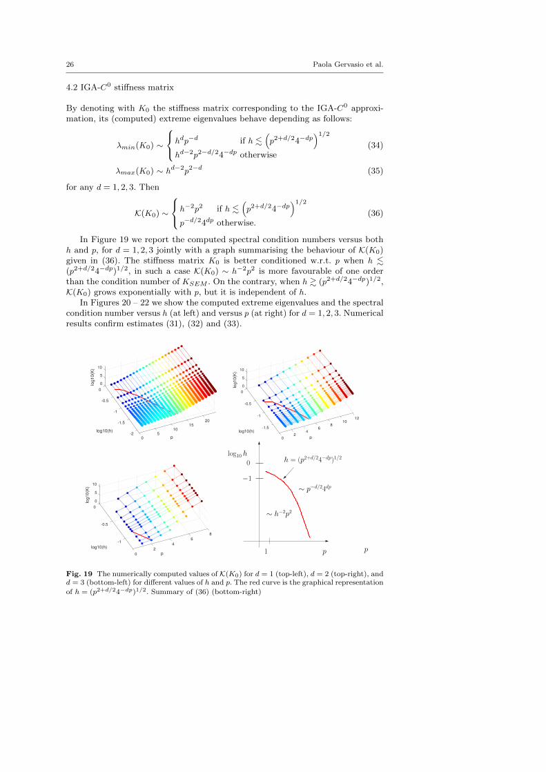
By denoting with K0 the stiffness matrix corresponding to the IGA-C0 approxi-mation, its (computed) extreme eigenvalues behave depending as follows:
λmin(K0) ∼
hdp−d if h .(p2+d/24−dp
)1/2hd−2p2−d/24−dp otherwise
(34)
λmax(K0) ∼ hd−2p2−d (35)
for any d = 1, 2, 3. Then
K(K0) ∼
h−2p2 if h .(p2+d/24−dp
)1/2p−d/24dp otherwise.
(36)
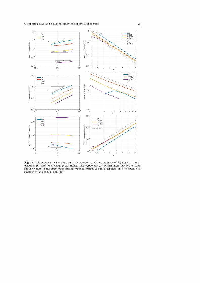
In Figure 19 we report the computed spectral condition numbers versus bothh and p, for d = 1, 2, 3 jointly with a graph summarising the behaviour of K(K0)given in (36). The stiffness matrix K0 is better conditioned w.r.t. p when h .(p2+d/24−dp)1/2, in such a case K(K0) ∼ h−2p2 is more favourable of one orderthan the condition number of KSEM . On the contrary, when h & (p2+d/24−dp)1/2,K(K0) grows exponentially with p, but it is independent of h.
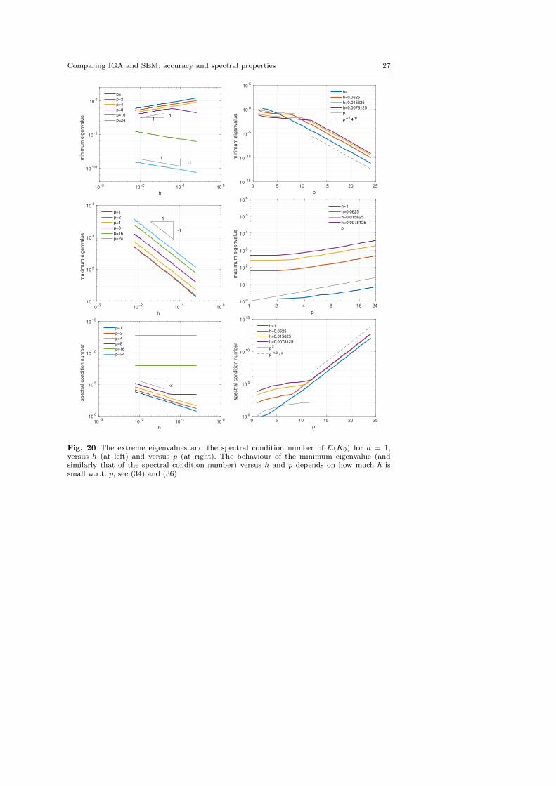
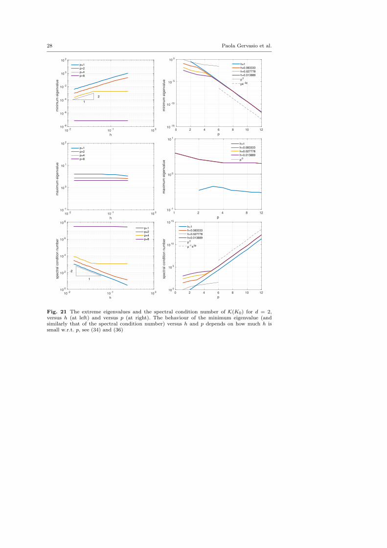
In Figures 20 – 22 we show the computed extreme eigenvalues and the spectralcondition number versus h (at left) and versus p (at right) for d = 1, 2, 3. Numericalresults confirm estimates (31), (32) and (33).
0
0
-0.5
-1
log10(h)
20-1.5
p
1510
5-2
5
0
log10(K
) 10
0
0
-0.5
log10(h)
-112
108
p
-1.5 64
2
5
0
log
10
(K)
10
0
0
-0.5
log10(h)
8
6
p
-14
2
0
5
log10(K
)
10
1 p
∼ h−2p2
0
−1
log10 h
p
h = (p2+d/24−dp)1/2
∼ p−d/24dp
Fig. 19 The numerically computed values of K(K0) for d = 1 (top-left), d = 2 (top-right), andd = 3 (bottom-left) for different values of h and p. The red curve is the graphical representation
of h = (p2+d/24−dp)1/2. Summary of (36) (bottom-right)
Comparing IGA and SEM: accuracy and spectral properties 27
10-3
10-2
10-1
100
h
10-10
10-5
100
min
imum
eig
envalu
e 11
-11
p=1
p=2
p=4
p=8
p=16
p=24
0 5 10 15 20 25
p
10-15
10-10
10-5
100
105
min
imum
eig
envalu
e
h=1
h=0.0625
h=0.015625
h=0.0078125
p
p3/2
4-p
10-3
10-2
10-1
100
h
101
102
103
104
maxim
um
eig
envalu
e
-1
1
p=1
p=2
p=4
p=8
p=16
p=24
1 2 4 8 16 24
p
100
101
102
103
104
105
106
maxim
um
eig
envalu
e
h=1
h=0.0625
h=0.015625
h=0.0078125
p
10-3
10-2
10-1
100
h
100
105
1010
1015
sp
ectr
al co
nd
itio
n n
um
be
r
-21
p=1
p=2
p=4
p=8
p=16
p=24
0 5 10 15 20 25
p
100
105
1010
1015
sp
ectr
al co
nd
itio
n n
um
be
r
h=1
h=0.0625
h=0.015625
h=0.0078125
p2
p-1/2
4p
Fig. 20 The extreme eigenvalues and the spectral condition number of K(K0) for d = 1,versus h (at left) and versus p (at right). The behaviour of the minimum eigenvalue (andsimilarly that of the spectral condition number) versus h and p depends on how much h issmall w.r.t. p, see (34) and (36)
28 Paola Gervasio et al.
10-2
10-1
100
h
10-8
10-6
10-4
10-2
100
102
min
imu
m e
ige
nva
lue
2
1
p=1
p=2
p=4
p=8
0 2 4 6 8 10 12
p
10-15
10-10
10-5
100
min
imum
eig
envalu
e
h=1
h=0.083333
h=0.027778
h=0.013889
p0
p4-2p
10-2
10-1
100
h
10-1
100
101
102
ma
xim
um
eig
en
va
lue
p=1
p=2
p=4
p=8
1 2 4 8 12
p
10-1
100
101
maxim
um
eig
envalu
e
h=1
h=0.083333
h=0.027778
h=0.013889
p0
10-2
10-1
100
h
100
102
104
106
108
spectr
al conditio
n n
um
ber
-2
1
p=1
p=2
p=4
p=8
0 2 4 6 8 10 12
p
100
105
1010
1015
sp
ectr
al co
nd
itio
n n
um
be
r
h=1
h=0.083333
h=0.027778
h=0.013889
p2
p-1
42p
Fig. 21 The extreme eigenvalues and the spectral condition number of K(K0) for d = 2,versus h (at left) and versus p (at right). The behaviour of the minimum eigenvalue (andsimilarly that of the spectral condition number) versus h and p depends on how much h issmall w.r.t. p, see (34) and (36)
Comparing IGA and SEM: accuracy and spectral properties 29
10-2
10-1
100
h
10-15
10-10
10-5
100
105
min
imum
eig
envalu
e 3
1
11
11
p=1
p=2
p=4
p=8
1 2 3 4 5 6 7 8
p
10-15
10-10
10-5
100
min
imum
eig
envalu
e
h=1
h=0.25
h=0.125
h=0.05
p-1
p1/2
4-3p
10-2
10-1
100
h
10-2
10-1
100
101
ma
xim
um
eig
en
va
lue
1
1
p=1
p=2
p=4
p=8
1 2 3 4 5 6 7 8
p
10 -2
10 -1
10 0
ma
xim
um
eig
en
va
lue
h=1
h=0.25
h=0.125
h=0.05
p-1
10-2
10-1
100
h
100
105
1010
sp
ectr
al co
nd
itio
n n
um
be
r
-2
1
p=1
p=2
p=4
p=8
1 2 3 4 5 6 7 8
p
100
105
1010
1015
spectr
al conditio
n n
um
ber
h=1
h=0.25
h=0.125
h=0.05
p2
p-3/2
43p
Fig. 22 The extreme eigenvalues and the spectral condition number of K(K0) for d = 3,versus h (at left) and versus p (at right). The behaviour of the minimum eigenvalue (andsimilarly that of the spectral condition number) versus h and p depends on how much h issmall w.r.t. p, see (34) and (36)
30 Paola Gervasio et al.
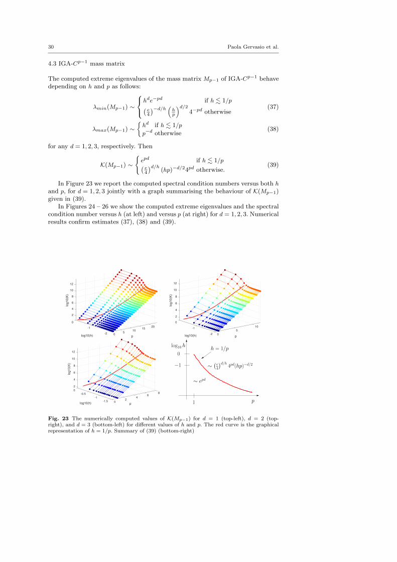
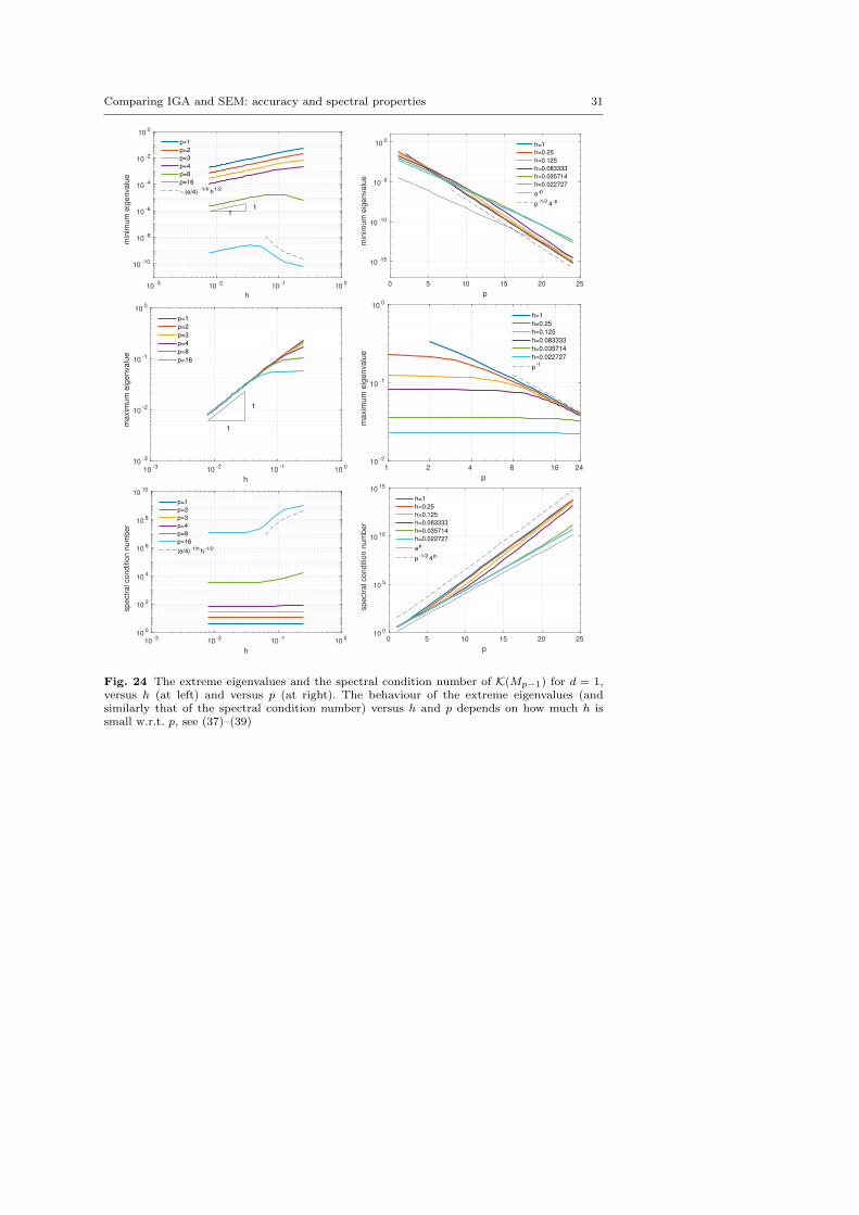
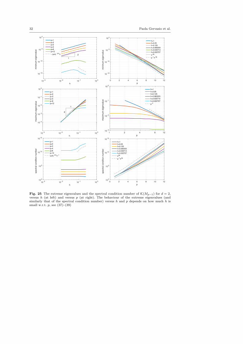
4.3 IGA-Cp−1 mass matrix
The computed extreme eigenvalues of the mass matrix Mp−1 of IGA-Cp−1 behavedepending on h and p as follows:
λmin(Mp−1) ∼
hde−pd if h . 1/p(e4
)−d/h (hp
)d/24−pd otherwise
(37)
λmax(Mp−1) ∼hd if h . 1/p
p−d otherwise(38)
for any d = 1, 2, 3, respectively. Then
K(Mp−1) ∼
epd if h . 1/p(e4
)d/h(hp)−d/24pd otherwise.
(39)
In Figure 23 we report the computed spectral condition numbers versus both hand p, for d = 1, 2, 3 jointly with a graph summarising the behaviour of K(Mp−1)given in (39).
In Figures 24 – 26 we show the computed extreme eigenvalues and the spectralcondition number versus h (at left) and versus p (at right) for d = 1, 2, 3. Numericalresults confirm estimates (37), (38) and (39).
2
0
4
6
8
log10(K
)
10
12
20
log10(h)
-1 15
p
105-2 0
2
0
4
6
8
log10(K
)
10
12
10
log10(h)
-1
p
5
-2 0
2
4
0
6
8
log
10
(K)
10
8
12
-0.5 6
log10(h) p
4-12
-1.5 0
0
−1
log10 h h = 1/p
∼(e4
)d/h4pd(hp)−d/2
∼ epd
1 p
Fig. 23 The numerically computed values of K(Mp−1) for d = 1 (top-left), d = 2 (top-right), and d = 3 (bottom-left) for different values of h and p. The red curve is the graphicalrepresentation of h = 1/p. Summary of (39) (bottom-right)
Comparing IGA and SEM: accuracy and spectral properties 31
10-3
10-2
10-1
100
h
10-10
10-8
10-6
10-4
10-2
100
min
imum
eig
envalu
e
11
p=1
p=2
p=3
p=4
p=8
p=16
(e/4)-1/h
h1/2
0 5 10 15 20 25
p
10-15
10-10
10-5
100
min
imum
eig
envalu
e
h=1
h=0.25
h=0.125
h=0.083333
h=0.035714
h=0.022727
e-p
p-1/2
4-p
10-3
10-2
10-1
100
h
10-3
10-2
10-1
100
ma
xim
um
eig
en
va
lue
1
1
p=1
p=2
p=3
p=4
p=8
p=16
1 2 4 8 16 24
p
10-2
10-1
100
maxim
um
eig
envalu
e
h=1
h=0.25
h=0.125
h=0.083333
h=0.035714
h=0.022727
p-1
10-3
10-2
10-1
100
h
100
102
104
106
108
1010
sp
ectr
al co
nd
itio
n n
um
be
r
p=1
p=2
p=3
p=4
p=8
p=16
(e/4)1/h
h-1/2
0 5 10 15 20 25
p
100
105
1010
1015
spectr
al conditio
n n
um
ber
h=1
h=0.25
h=0.125
h=0.083333
h=0.035714
h=0.022727
ep
p-1/2
4p
Fig. 24 The extreme eigenvalues and the spectral condition number of K(Mp−1) for d = 1,versus h (at left) and versus p (at right). The behaviour of the extreme eigenvalues (andsimilarly that of the spectral condition number) versus h and p depends on how much h issmall w.r.t. p, see (37)–(39)
32 Paola Gervasio et al.
10-3
10-2
10-1
100
h
10-15
10-10
10-5
100
min
imum
eig
envalu
e
2
1
p=1
p=2
p=3
p=4
p=8
p=12
(e/4)-2/h
h
0 2 4 6 8 10 12
p
10-15
10-10
10-5
100
min
imum
eig
envalu
e
h=1
h=0.25
h=0.125
h=0.083333
h=0.035714
h=0.022727
e-2p
p-1
4-2p
10-3
10-2
10-1
100
h
10-4
10-3
10-2
10-1
100
ma
xim
um
eig
en
va
lue
2
1
p=1
p=2
p=3
p=4
p=8
p=12
1 2 4 8 12
p
10-3
10-2
10-1
100
maxim
um
eig
envalu
e
h=1
h=0.25
h=0.125
h=0.083333
h=0.035714
h=0.022727
p-2
10-3
10-2
10-1
100
h
100
105
1010
1015
sp
ectr
al co
nd
itio
n n
um
be
r
p=1
p=2
p=3
p=4
p=8
p=12
(e/4)2/h
h-1
0 2 4 6 8 10 12
p
100
105
1010
1015
spectr
al conditio
n n
um
ber
h=1
h=0.25
h=0.125
h=0.083333
h=0.035714
h=0.022727
e2p
p-1
42p
Fig. 25 The extreme eigenvalues and the spectral condition number of K(Mp−1) for d = 2,versus h (at left) and versus p (at right). The behaviour of the extreme eigenvalues (andsimilarly that of the spectral condition number) versus h and p depends on how much h issmall w.r.t. p, see (37)–(39)
Comparing IGA and SEM: accuracy and spectral properties 33
10-2
10-1
100
h
10-15
10-10
10-5
100
min
imum
eig
envalu
e
3
1
p=1
p=2
p=3
p=4
p=8
(e/4)-3/h
h3/2
0 2 4 6 8
p
10-15
10-10
10-5
100
min
imum
eig
envalu
e
h=1
h=0.5
h=0.33333
h=0.25
h=0.125
h=0.083333
e-3p
p-3/2
4-3p
10-2
10-1
100
h
10-5
10-4
10-3
10-2
10-1
ma
xim
um
eig
en
va
lue
3
1
p=1
p=2
p=3
p=4
p=8
1 2 4 8
p
10-4
10-3
10-2
10-1
100
maxim
um
eig
envalu
e
h=1
h=0.5
h=0.33333
h=0.25
h=0.125
h=0.083333
p-3
10-2
10-1
100
h
100
105
1010
1015
sp
ectr
al co
nd
itio
n n
um
be
r
p=1
p=2
p=3
p=4
p=8
(e/4)3/h
h-3/2
1 2 3 4 5 6 7 8
p
100
105
1010
1015
spectr
al conditio
n n
um
ber
h=1
h=0.5
h=0.33333
h=0.25
h=0.125
h=0.083333
e3p
p-3/2
43p
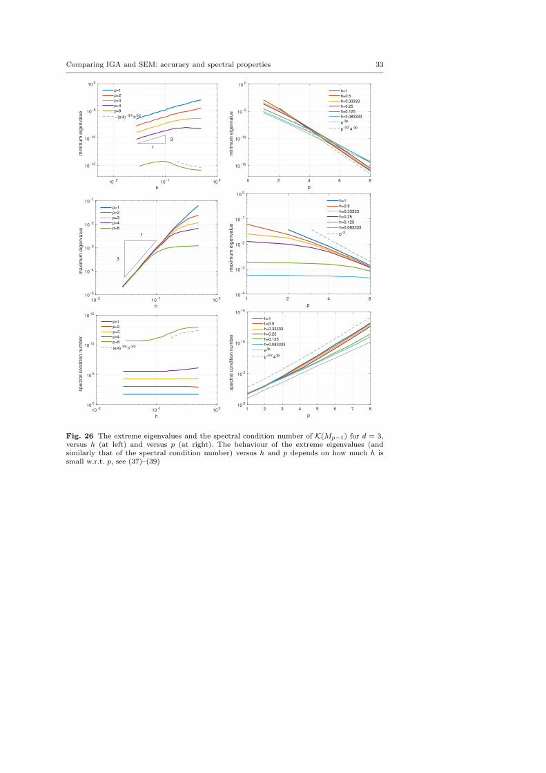
Fig. 26 The extreme eigenvalues and the spectral condition number of K(Mp−1) for d = 3,versus h (at left) and versus p (at right). The behaviour of the extreme eigenvalues (andsimilarly that of the spectral condition number) versus h and p depends on how much h issmall w.r.t. p, see (37)–(39)
34 Paola Gervasio et al.
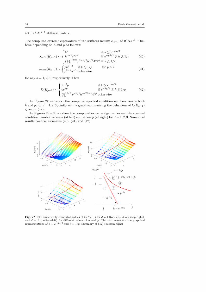
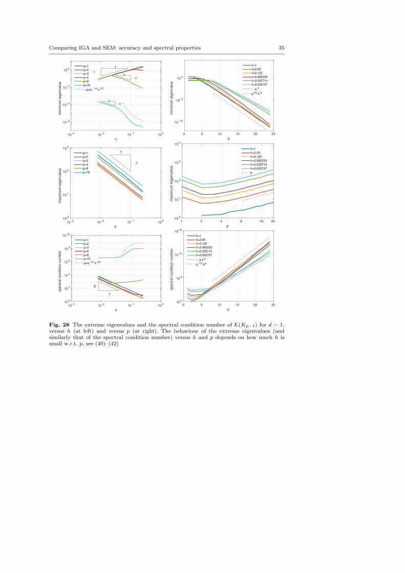
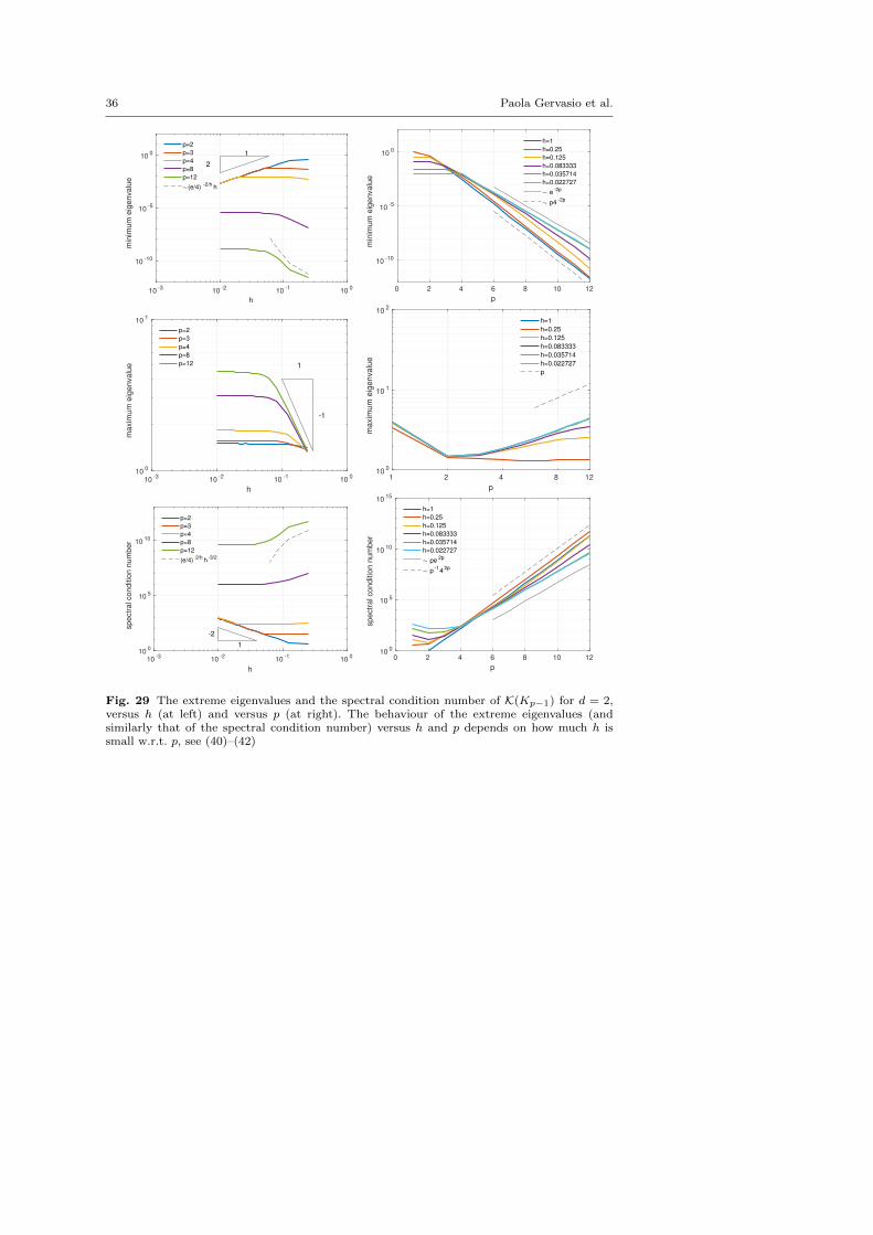
4.4 IGA-Cp−1 stiffness matrix
The computed extreme eigenvalues of the stiffness matrix Kp−1 of IGA-Cp−1 be-have depending on h and p as follows:
λmin(Kp−1) ∼
hd if h . e−pd/2
hd−2e−pd if e−pd/2 . h . 1/p(e4
)−d/hp2−d/2hd/24−pd if h & 1/p
(40)
λmax(Kp−1) ∼phd−2 if h . 1/p for p > 2
p2−dh−1 otherwise.(41)
for any d = 1, 2, 3, respectively. Then
K(Kp−1) ∼
h−2p if h . e−dp/2
pedp if e−dp/2 . h . 1/p(e4
)d/hp−d/2h−d/2−14dp otherwise
(42)
In Figure 27 we report the computed spectral condition numbers versus bothh and p, for d = 1, 2, 3 jointly with a graph summarising the behaviour of K(Kp−1)given in (42).
In Figures 28 – 30 we show the computed extreme eigenvalues and the spectralcondition number versus h (at left) and versus p (at right) for d = 1, 2, 3. Numericalresults confirm estimates (40), (41) and (42).
0
0
20-0.5
5
15
log10(h)
-1
p
log10(K
)
10-1.5
5
10
-2 0
0
0
10-0.5
5
log10(h) p
-1
log10(K
)
5-1.5
10
-2 0
0
0 8
6-0.5
log10(h)
5
p
4
log
10
(K)
-12
-1.5 0
10
∼ h−2p
log10 h
h = e−dp/2
∼ pedp
p1
−1
0 ∼(e4
)d/hp−d/2h−d/2−14dp
h = 1/p
1 2
3
Fig. 27 The numerically computed values of K(Kp−1) for d = 1 (top-left), d = 2 (top-right),and d = 3 (bottom-left) for different values of h and p. The red curves are the graphical
representations of h = e−dp/2 and h = 1/p. Summary of (42) (bottom-right)
Comparing IGA and SEM: accuracy and spectral properties 35
10-3
10-2
10-1
100
h
10-6
10-4
10-2
100
min
imu
m e
ige
nva
lue
1
1
-11
-11
p=1
p=2
p=3
p=4
p=8
p=16
(e/4)-1/h
h1/2
0 5 10 15 20 25
p
10-10
10-5
100
min
imum
eig
envalu
e
h=1
h=0.25
h=0.125
h=0.083333
h=0.035714
h=0.022727
e-p
p3/2
4-p
10-3
10-2
10-1
100
h
100
101
102
103
maxim
um
eig
envalu
e
-1
1p=1
p=2
p=3
p=4
p=8
p=16
1 2 4 8 16 24
p
100
101
102
103
104
maxim
um
eig
envalu
e
h=1
h=0.25
h=0.125
h=0.083333
h=0.035714
h=0.022727
p
10-3
10-2
10-1
100
h
100
102
104
106
108
1010
sp
ectr
al co
nd
itio
n n
um
be
r
-2
1
p=1
p=2
p=3
p=4
p=8
p=16
(e/4)1/h
h-3/2
0 5 10 15 20 25
p
100
105
1010
1015
sp
ectr
al co
nd
itio
n n
um
be
r
h=1
h=0.25
h=0.125
h=0.083333
h=0.035714
h=0.022727
p ep
p-1/2
4p
Fig. 28 The extreme eigenvalues and the spectral condition number of K(Kp−1) for d = 1,versus h (at left) and versus p (at right). The behaviour of the extreme eigenvalues (andsimilarly that of the spectral condition number) versus h and p depends on how much h issmall w.r.t. p, see (40)–(42)
36 Paola Gervasio et al.
10-3
10-2
10-1
100
h
10-10
10-5
100
min
imum
eig
envalu
e
2
1
p=2
p=3
p=4
p=8
p=12
(e/4)-2/h
h
0 2 4 6 8 10 12
p
10-10
10-5
100
min
imum
eig
envalu
e
h=1
h=0.25
h=0.125
h=0.083333
h=0.035714
h=0.022727
e-2p
p4-2p
10-3
10-2
10-1
100
h
100
101
maxim
um
eig
envalu
e
-1
1
p=2
p=3
p=4
p=8
p=12
1 2 4 8 12
p
100
101
102
maxim
um
eig
envalu
e
h=1
h=0.25
h=0.125
h=0.083333
h=0.035714
h=0.022727
p
10-3
10-2
10-1
100
h
100
105
1010
sp
ectr
al co
nd
itio
n n
um
be
r
-2
1
p=2
p=3
p=4
p=8
p=12
(e/4)2/h
h-3/2
0 2 4 6 8 10 12
p
100
105
1010
1015
sp
ectr
al co
nd
itio
n n
um
be
r
h=1
h=0.25
h=0.125
h=0.083333
h=0.035714
h=0.022727
pe2p
p-1
42p
Fig. 29 The extreme eigenvalues and the spectral condition number of K(Kp−1) for d = 2,versus h (at left) and versus p (at right). The behaviour of the extreme eigenvalues (andsimilarly that of the spectral condition number) versus h and p depends on how much h issmall w.r.t. p, see (40)–(42)
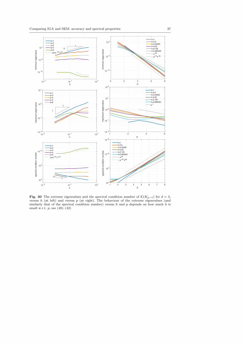
Comparing IGA and SEM: accuracy and spectral properties 37
10-2
10-1
100
h
10-10
10-5
100
min
imum
eig
envalu
e
3
1
p=1
p=2
p=3
p=4
p=8
(e/4)-3/h
h3/2
0 2 4 6 8
p
10-10
10-5
100
min
imum
eig
envalu
e
h=1
h=0.5
h=0.33333
h=0.25
h=0.125
h=0.083333
e-3p
p1/2
4-3p
10-2
10-1
100
h
10-2
10-1
100
101
ma
xim
um
eig
en
va
lue
1
1
p=1
p=2
p=3
p=4
p=8
1 2 4 8
p
10-2
10-1
100
101
102
maxim
um
eig
envalu
e
h=1
h=0.5
h=0.33333
h=0.25
h=0.125
h=0.083333
p-1
10-2
10-1
100
h
100
105
1010
sp
ectr
al co
nd
itio
n n
um
be
r
-21
p=1
p=2
p=3
p=4
p=8
(e/4)3/h
h-5/2
1 2 3 4 5 6 7 8
p
100
105
1010
1015
spectr
al conditio
n n
um
ber
h=1
h=0.5
h=0.33333
h=0.25
h=0.125
h=0.083333
e3p
p-3/2
43p
Fig. 30 The extreme eigenvalues and the spectral condition number of K(Kp−1) for d = 3,versus h (at left) and versus p (at right). The behaviour of the extreme eigenvalues (andsimilarly that of the spectral condition number) versus h and p depends on how much h issmall w.r.t. p, see (40)–(42)
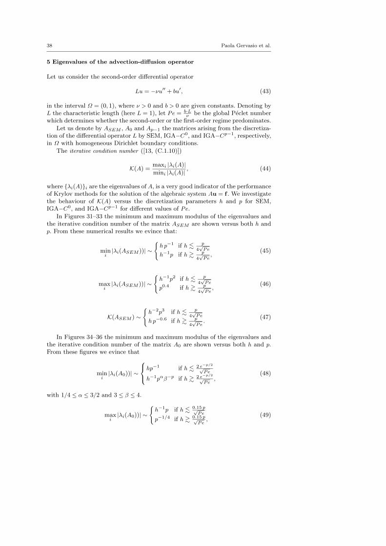
38 Paola Gervasio et al.
5 Eigenvalues of the advection-diffusion operator
Let us consider the second-order differential operator
Lu = −νu′′ + bu′, (43)
in the interval Ω = (0, 1), where ν > 0 and b > 0 are given constants. Denoting byL the characteristic length (here L = 1), let Pe = b·L
ν be the global Peclet numberwhich determines whether the second-order or the first-order regime predominates.
Let us denote by ASEM , A0 and Ap−1 the matrices arising from the discretiza-tion of the differential operator L by SEM, IGA−C0, and IGA−Cp−1, respectively,in Ω with homogeneous Dirichlet boundary conditions.
The iterative condition number ([13, (C.1.10)])
K(A) =maxi |λi(A)|mini |λi(A)|
, (44)
where λi(A)i are the eigenvalues of A, is a very good indicator of the performanceof Krylov methods for the solution of the algebraic system Au = f . We investigatethe behaviour of K(A) versus the discretization parameters h and p for SEM,IGA−C0, and IGA−Cp−1 for different values of Pe.
In Figures 31–33 the minimum and maximum modulus of the eigenvalues andthe iterative condition number of the matrix ASEM are shown versus both h andp. From these numerical results we evince that:
mini|λi(ASEM ))| ∼
h p−1 if h . p
4√Pe
h−1p if h & p
4√Pe,
(45)
maxi|λi(ASEM ))| ∼
h−1p2 if h . p
4√Pe
p0.4 if h & p
4√Pe,
(46)
K(ASEM ) ∼
h−2p3 if h . p
4√Pe
h p−0.6 if h & p
4√Pe.
(47)
In Figures 34–36 the minimum and maximum modulus of the eigenvalues andthe iterative condition number of the matrix A0 are shown versus both h and p.From these figures we evince that
mini|λi(A0))| ∼
hp−1 if h . 2 e−p/2√Pe
h−1pαβ−p if h & 2 e−p/2√Pe
,(48)
with 1/4 ≤ α ≤ 3/2 and 3 ≤ β ≤ 4.
maxi|λi(A0))| ∼
h−1p if h . 0.15 p√
Pe
p−1/4 if h & 0.15 p√Pe
,(49)
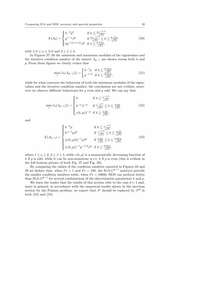
Comparing IGA and SEM: accuracy and spectral properties 39
K(A0) ∼
h−2p2 if h . 2 e−p/2√
Pe
p1−αβp if 2 e−p/2√Pe
. h . 0.15 p√Pe
hp−(α+1/4)βp if h & 0.15 p√Pe
,
(50)
with 1/4 ≤ α ≤ 3/2 and 3 ≤ β ≤ 4.In Figures 37–39 the minimum and maximum modulus of the eigenvalues and
the iterative condition number of the matrix Ap−1 are shown versus both h andp. From these figures we clearly evince that
maxi|λi(Ap−1))| ∼
h−1p if h . 0.05 p√
Pe
p−1/2 if h & 0.05 p√Pe
,(51)
while for what concerns the behaviour of both the minimum modulus of the eigen-values and the iterative condition number, the conclusions are not evident, more-over we observe different behaviours for p even and p odd. We can say that
mini|λi(Ap−1))| ∼
h if h . e−p/2√
Pe
h−αβ−p if e−p/2√Pe
. h . 0.05√Pe
c(h, p)β−p if h & 0.05√Pe,
(52)
and
K(Ap−1) ∼
h−2p if h . e−p/2√Pe
hα−1pβp if e−p/2√Pe
. h . 0.05√Pe
(c(h, p)h)−1pβp if 0.05√Pe
. h . 0.05 p√Pe
(c(h, p))−1p−1/2βp if h & 0.05 p√Pe
,
(53)
where 1 ≤ α ≤ 2, 2 ≤ β ≤ 4, while c(h, p) is a monotonically decreasing function ofh if p is odd, while it can be non-monotone w.r.t. h if p is even (this is evident inthe left-bottom picture of both Fig. 37 and Fig. 39).
By comparing the values of the condition numbers reported in Figures 33 and39 we deduce that, when Pe = 1 and Pe = 100, the IGA-Cp−1 matrices providethe smaller condition numbers while, when Pe = 10000, SEM can perform betterthan IGA-Cp−1 for several combinations of the discretization parameters h and p.
We warn the reader that the results of this section refer to the case d = 1 and,more in general, in accordance with the numerical results shown in the previoussection for the Poisson problem, we expect that βp should be replaced by βpd inboth (52) and (53).
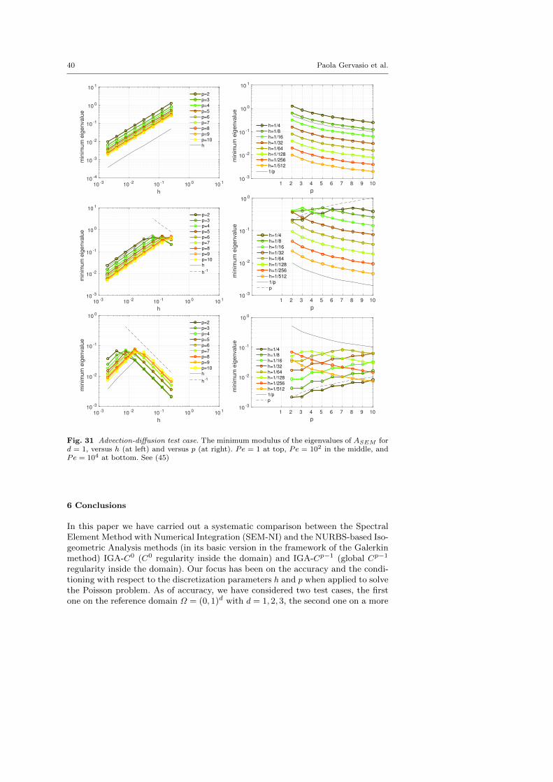
40 Paola Gervasio et al.
10-3
10-2
10-1
100
101
h
10-4
10-3
10-2
10-1
100
101
min
imu
m e
ige
nva
lue
p=2
p=3
p=4
p=5
p=6
p=7
p=8
p=9
p=10
h
1 2 3 4 5 6 7 8 9 10
p
10-3
10-2
10-1
100
101
min
imum
eig
envalu
e
h=1/4
h=1/8
h=1/16
h=1/32
h=1/64
h=1/128
h=1/256
h=1/512
1/p
10-3
10-2
10-1
100
101
h
10-3
10-2
10-1
100
101
min
imu
m e
ige
nva
lue
p=2
p=3
p=4
p=5
p=6
p=7
p=8
p=9
p=10
h
h-1
1 2 3 4 5 6 7 8 9 10
p
10-3
10-2
10-1
100
min
imu
m e
ige
nva
lue
h=1/4
h=1/8
h=1/16
h=1/32
h=1/64
h=1/128
h=1/256
h=1/512
1/p
p
10-3
10-2
10-1
100
101
h
10-3
10-2
10-1
100
min
imu
m e
ige
nva
lue
p=2
p=3
p=4
p=5
p=6
p=7
p=8
p=9
p=10
h
h-1
1 2 3 4 5 6 7 8 9 10
p
10-3
10-2
10-1
100
min
imum
eig
envalu
e
h=1/4
h=1/8
h=1/16
h=1/32
h=1/64
h=1/128
h=1/256
h=1/512
1/p
p
Fig. 31 Advection-diffusion test case. The minimum modulus of the eigenvalues of ASEM ford = 1, versus h (at left) and versus p (at right). Pe = 1 at top, Pe = 102 in the middle, andPe = 104 at bottom. See (45)
6 Conclusions
In this paper we have carried out a systematic comparison between the SpectralElement Method with Numerical Integration (SEM-NI) and the NURBS-based Iso-geometric Analysis methods (in its basic version in the framework of the Galerkinmethod) IGA-C0 (C0 regularity inside the domain) and IGA-Cp−1 (global Cp−1
regularity inside the domain). Our focus has been on the accuracy and the condi-tioning with respect to the discretization parameters h and p when applied to solvethe Poisson problem. As of accuracy, we have considered two test cases, the firstone on the reference domain Ω = (0, 1)d with d = 1, 2, 3, the second one on a more
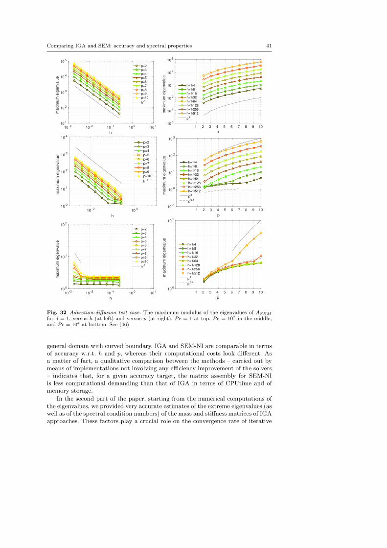
Comparing IGA and SEM: accuracy and spectral properties 41
10-3
10-2
10-1
100
101
h
101
102
103
104
105
ma
xim
um
eig
en
va
lue
p=2
p=3
p=4
p=5
p=6
p=7
p=8
p=9
p=10
h-1
1 2 3 4 5 6 7 8 9 10
p
100
101
102
103
104
105
ma
xim
um
eig
en
va
lue
h=1/4
h=1/8
h=1/16
h=1/32
h=1/64
h=1/128
h=1/256
h=1/512
p2
10-2
100
h
100
101
102
103
104
ma
xim
um
eig
en
va
lue
p=2
p=3
p=4
p=5
p=6
p=7
p=8
p=9
p=10
h-1
1 2 3 4 5 6 7 8 9 10
p
10-1
100
101
102
103
ma
xim
um
eig
en
va
lue
h=1/4
h=1/8
h=1/16
h=1/32
h=1/64
h=1/128
h=1/256
h=1/512
p2
p0.4
10-3
10-2
10-1
100
101
h
100
101
102
maxim
um
eig
envalu
e
p=2
p=3
p=4
p=5
p=6
p=7
p=8
p=9
p=10
h-1
1 2 3 4 5 6 7 8 9 10
p
100
101
maxim
um
eig
envalu
e
h=1/4
h=1/8
h=1/16
h=1/32
h=1/64
h=1/128
h=1/256
h=1/512
p2
p0.4
Fig. 32 Advection-diffusion test case. The maximum modulus of the eigenvalues of ASEMfor d = 1, versus h (at left) and versus p (at right). Pe = 1 at top, Pe = 102 in the middle,and Pe = 104 at bottom. See (46)
general domain with curved boundary. IGA and SEM-NI are comparable in termsof accuracy w.r.t. h and p, whereas their computational costs look different. Asa matter of fact, a qualitative comparison between the methods – carried out bymeans of implementations not involving any efficiency improvement of the solvers– indicates that, for a given accuracy target, the matrix assembly for SEM-NIis less computational demanding than that of IGA in terms of CPUtime and ofmemory storage.
In the second part of the paper, starting from the numerical computations ofthe eigenvalues, we provided very accurate estimates of the extreme eigenvalues (aswell as of the spectral condition numbers) of the mass and stiffness matrices of IGAapproaches. These factors play a crucial role on the convergence rate of iterative
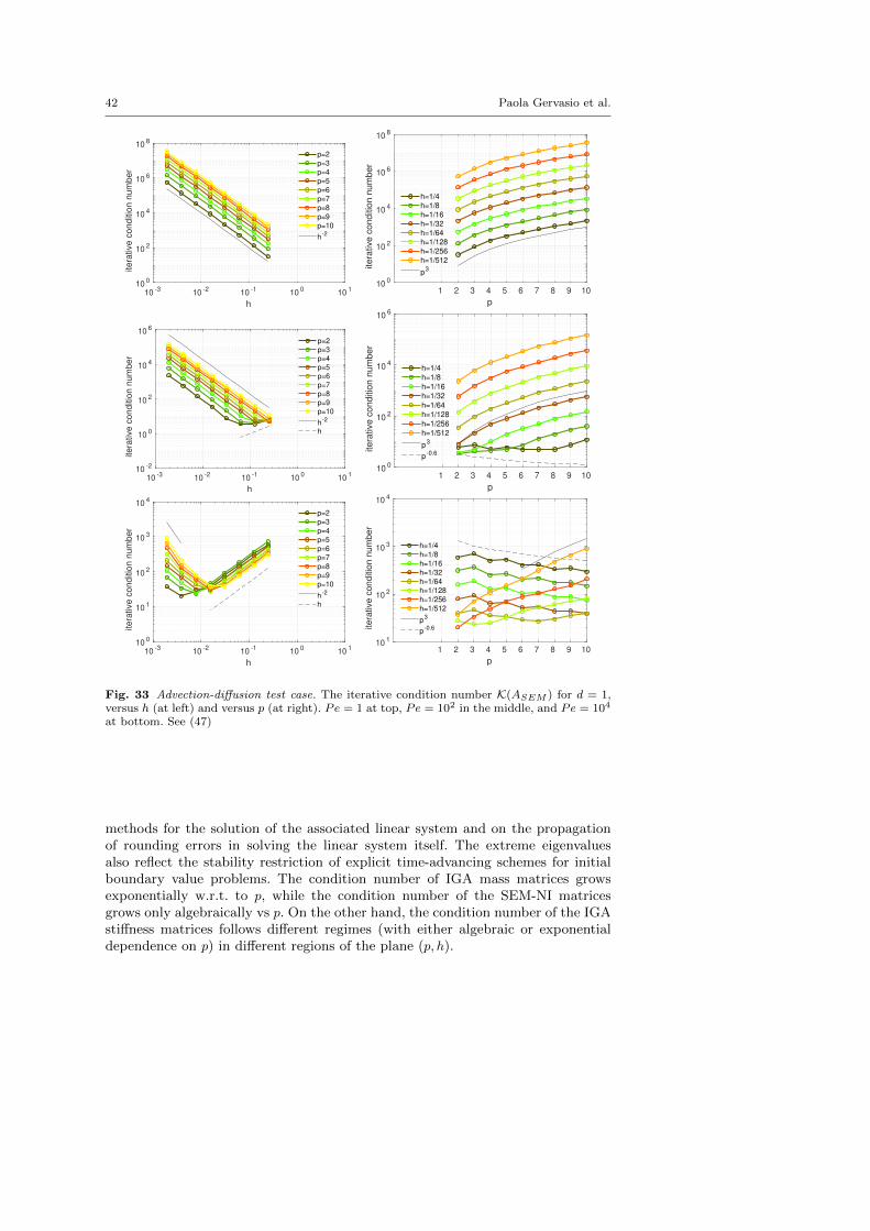
42 Paola Gervasio et al.
10-3
10-2
10-1
100
101
h
100
102
104
106
108
ite
rative
co
nd
itio
n n
um
be
r
p=2
p=3
p=4
p=5
p=6
p=7
p=8
p=9
p=10
h-2
1 2 3 4 5 6 7 8 9 10
p
100
102
104
106
108
itera
tive c
onditio
n n
um
ber
h=1/4
h=1/8
h=1/16
h=1/32
h=1/64
h=1/128
h=1/256
h=1/512
p3
10-3
10-2
10-1
100
101
h
10-2
100
102
104
106
ite
rative
co
nd
itio
n n
um
be
r
p=2
p=3
p=4
p=5
p=6
p=7
p=8
p=9
p=10
h-2
h
1 2 3 4 5 6 7 8 9 10
p
100
102
104
106
itera
tive c
onditio
n n
um
ber
h=1/4
h=1/8
h=1/16
h=1/32
h=1/64
h=1/128
h=1/256
h=1/512
p3
p-0.6
10-3
10-2
10-1
100
101
h
100
101
102
103
104
ite
rative
co
nd
itio
n n
um
be
r
p=2
p=3
p=4
p=5
p=6
p=7
p=8
p=9
p=10
h-2
h
1 2 3 4 5 6 7 8 9 10
p
101
102
103
104
ite
rative
co
nd
itio
n n
um
be
r
h=1/4
h=1/8
h=1/16
h=1/32
h=1/64
h=1/128
h=1/256
h=1/512
p3
p-0.6
Fig. 33 Advection-diffusion test case. The iterative condition number K(ASEM ) for d = 1,versus h (at left) and versus p (at right). Pe = 1 at top, Pe = 102 in the middle, and Pe = 104
at bottom. See (47)
methods for the solution of the associated linear system and on the propagationof rounding errors in solving the linear system itself. The extreme eigenvaluesalso reflect the stability restriction of explicit time-advancing schemes for initialboundary value problems. The condition number of IGA mass matrices growsexponentially w.r.t. to p, while the condition number of the SEM-NI matricesgrows only algebraically vs p. On the other hand, the condition number of the IGAstiffness matrices follows different regimes (with either algebraic or exponentialdependence on p) in different regions of the plane (p, h).
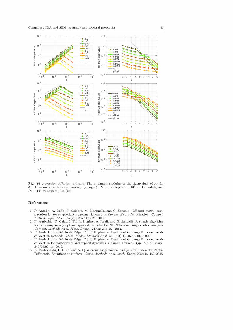
Comparing IGA and SEM: accuracy and spectral properties 43
10-3
10-2
10-1
100
101
h
10-3
10-2
10-1
100
101
min
imu
m e
ige
nva
lue
p=2
p=3
p=4
p=5
p=6
p=7
p=8
p=9
p=10
h
h-1
2 3 4 5 6 7 8 9 10
p
10-3
10-2
10-1
100
101
min
imum
eig
envalu
e
h=1/4
h=1/8
h=1/16
h=1/32
h=1/64
h=1/128
h=1/256
h=1/512
1/p
p3/2
4-p
10-3
10-2
10-1
100
101
h
10-5
10-4
10-3
10-2
10-1
100
min
imu
m e
ige
nva
lue
p=2
p=3
p=4
p=5
p=6
p=7
p=8
p=9
p=10
h
h-1
2 3 4 5 6 7 8 9 10
p
10-5
10-4
10-3
10-2
10-1
100
min
imum
eig
envalu
e h=1/4
h=1/8
h=1/16
h=1/32
h=1/64
h=1/128
h=1/256
h=1/512
1/p
p3/2
4-p
p1/4
3-p
10-3
10-2
10-1
100
101
h
10-8
10-6
10-4
10-2
100
min
imu
m e
ige
nva
lue
p=2
p=3
p=4
p=5
p=6
p=7
p=8
p=9
p=10
h-1
2 3 4 5 6 7 8 9 10
p
10-8
10-6
10-4
10-2
100
min
imum
eig
envalu
e
h=1/4
h=1/8
h=1/16
h=1/32
h=1/64
h=1/128
h=1/256
h=1/512
p1/4
3-p
Fig. 34 Advection-diffusion test case. The minimum modulus of the eigenvalues of A0 ford = 1, versus h (at left) and versus p (at right). Pe = 1 at top, Pe = 102 in the middle, andPe = 104 at bottom. See (48)
References
1. P. Antolin, A. Buffa, F. Calabro, M. Martinelli, and G. Sangalli. Efficient matrix com-putation for tensor-product isogeometric analysis: the use of sum factorization. Comput.Methods Appl. Mech. Engrg., 285:817–828, 2015.
2. F. Auricchio, F. Calabro, T.J.R. Hughes, A. Reali, and G. Sangalli. A simple algorithmfor obtaining nearly optimal quadrature rules for NURBS-based isogeometric analysis.Comput. Methods Appl. Mech. Engrg., 249/252:15–27, 2012.
3. F. Auricchio, L. Beirao da Veiga, T.J.R. Hughes, A. Reali, and G. Sangalli. Isogeometriccollocation methods. Math. Models Methods Appl. Sci., 20(11):2075–2107, 2010.
4. F. Auricchio, L. Beirao da Veiga, T.J.R. Hughes, A. Reali, and G. Sangalli. Isogeometriccollocation for elastostatics and explicit dynamics. Comput. Methods Appl. Mech. Engrg.,249/252:2–14, 2012.
5. A. Bartezzaghi, L. Dede, and A. Quarteroni. Isogeometric Analysis for high order PartialDifferential Equations on surfaces. Comp. Methods Appl. Mech. Engrg, 295:446–469, 2015.
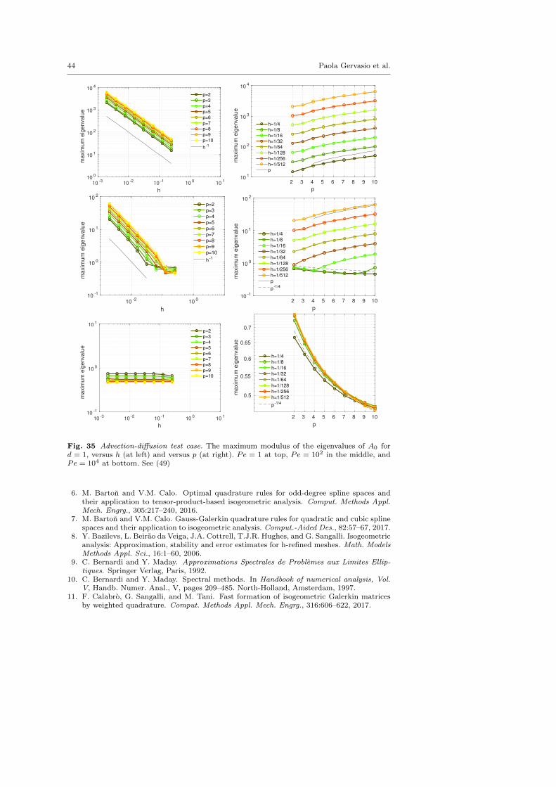
44 Paola Gervasio et al.
10-3
10-2
10-1
100
101
h
100
101
102
103
104
ma
xim
um
eig
en
va
lue
p=2
p=3
p=4
p=5
p=6
p=7
p=8
p=9
p=10
h-1
2 3 4 5 6 7 8 9 10
p
101
102
103
104
ma
xim
um
eig
en
va
lue
h=1/4
h=1/8
h=1/16
h=1/32
h=1/64
h=1/128
h=1/256
h=1/512
p
10-2
100
h
10-1
100
101
102
maxim
um
eig
envalu
e
p=2
p=3
p=4
p=5
p=6
p=7
p=8
p=9
p=10
h-1
2 3 4 5 6 7 8 9 10
p
10-1
100
101
102
ma
xim
um
eig
en
va
lue
h=1/4
h=1/8
h=1/16
h=1/32
h=1/64
h=1/128
h=1/256
h=1/512
p
p-1/4
10-3
10-2
10-1
100
101
h
10-1
100
101
ma
xim
um
eig
en
va
lue
p=2
p=3
p=4
p=5
p=6
p=7
p=8
p=9
p=10
2 3 4 5 6 7 8 9 10
p
0.5
0.55
0.6
0.65
0.7
ma
xim
um
eig
en
va
lue
h=1/4
h=1/8
h=1/16
h=1/32
h=1/64
h=1/128
h=1/256
h=1/512
p-1/4
Fig. 35 Advection-diffusion test case. The maximum modulus of the eigenvalues of A0 ford = 1, versus h (at left) and versus p (at right). Pe = 1 at top, Pe = 102 in the middle, andPe = 104 at bottom. See (49)
6. M. Barton and V.M. Calo. Optimal quadrature rules for odd-degree spline spaces andtheir application to tensor-product-based isogeometric analysis. Comput. Methods Appl.Mech. Engrg., 305:217–240, 2016.
7. M. Barton and V.M. Calo. Gauss-Galerkin quadrature rules for quadratic and cubic splinespaces and their application to isogeometric analysis. Comput.-Aided Des., 82:57–67, 2017.
8. Y. Bazilevs, L. Beirao da Veiga, J.A. Cottrell, T.J.R. Hughes, and G. Sangalli. Isogeometricanalysis: Approximation, stability and error estimates for h-refined meshes. Math. ModelsMethods Appl. Sci., 16:1–60, 2006.
9. C. Bernardi and Y. Maday. Approximations Spectrales de Problemes aux Limites Ellip-tiques. Springer Verlag, Paris, 1992.
10. C. Bernardi and Y. Maday. Spectral methods. In Handbook of numerical analysis, Vol.V, Handb. Numer. Anal., V, pages 209–485. North-Holland, Amsterdam, 1997.
11. F. Calabro, G. Sangalli, and M. Tani. Fast formation of isogeometric Galerkin matricesby weighted quadrature. Comput. Methods Appl. Mech. Engrg., 316:606–622, 2017.
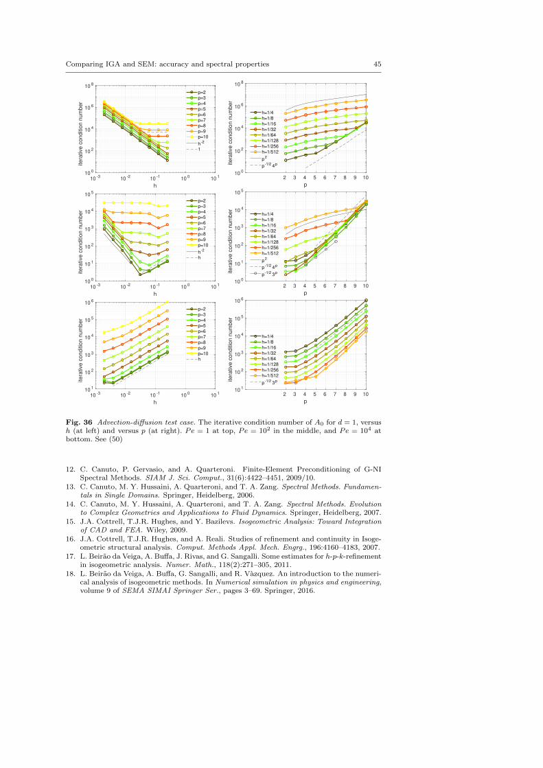
Comparing IGA and SEM: accuracy and spectral properties 45
10-3
10-2
10-1
100
101
h
100
102
104
106
108
ite
rative
co
nd
itio
n n
um
be
r
p=2
p=3
p=4
p=5
p=6
p=7
p=8
p=9
p=10
h-2
1
2 3 4 5 6 7 8 9 10
p
100
102
104
106
108
ite
rative
co
nd
itio
n n
um
be
r
h=1/4
h=1/8
h=1/16
h=1/32
h=1/64
h=1/128
h=1/256
h=1/512
p2
p-1/2
4p
10-3
10-2
10-1
100
101
h
100
101
102
103
104
105
ite
rative
co
nd
itio
n n
um
be
r
p=2
p=3
p=4
p=5
p=6
p=7
p=8
p=9
p=10
h-2
h
2 3 4 5 6 7 8 9 10
p
100
101
102
103
104
105
ite
rative
co
nd
itio
n n
um
be
r
h=1/4
h=1/8
h=1/16
h=1/32
h=1/64
h=1/128
h=1/256
h=1/512
p2
p-1/2
4p
p-1/2
3p
10-3
10-2
10-1
100
101
h
101
102
103
104
105
106
ite
rative
co
nd
itio
n n
um
be
r
p=2
p=3
p=4
p=5
p=6
p=7
p=8
p=9
p=10
h
2 3 4 5 6 7 8 9 10
p
101
102
103
104
105
106
ite
rative
co
nd
itio
n n
um
be
r
h=1/4
h=1/8
h=1/16
h=1/32
h=1/64
h=1/128
h=1/256
h=1/512
p-1/2
3p
Fig. 36 Advection-diffusion test case. The iterative condition number of A0 for d = 1, versush (at left) and versus p (at right). Pe = 1 at top, Pe = 102 in the middle, and Pe = 104 atbottom. See (50)
12. C. Canuto, P. Gervasio, and A. Quarteroni. Finite-Element Preconditioning of G-NISpectral Methods. SIAM J. Sci. Comput., 31(6):4422–4451, 2009/10.
13. C. Canuto, M. Y. Hussaini, A. Quarteroni, and T. A. Zang. Spectral Methods. Fundamen-tals in Single Domains. Springer, Heidelberg, 2006.
14. C. Canuto, M. Y. Hussaini, A. Quarteroni, and T. A. Zang. Spectral Methods. Evolutionto Complex Geometries and Applications to Fluid Dynamics. Springer, Heidelberg, 2007.
15. J.A. Cottrell, T.J.R. Hughes, and Y. Bazilevs. Isogeometric Analysis: Toward Integrationof CAD and FEA. Wiley, 2009.
16. J.A. Cottrell, T.J.R. Hughes, and A. Reali. Studies of refinement and continuity in Isoge-ometric structural analysis. Comput. Methods Appl. Mech. Engrg., 196:4160–4183, 2007.
17. L. Beirao da Veiga, A. Buffa, J. Rivas, and G. Sangalli. Some estimates for h-p-k-refinementin isogeometric analysis. Numer. Math., 118(2):271–305, 2011.
18. L. Beirao da Veiga, A. Buffa, G. Sangalli, and R. Vazquez. An introduction to the numeri-cal analysis of isogeometric methods. In Numerical simulation in physics and engineering,volume 9 of SEMA SIMAI Springer Ser., pages 3–69. Springer, 2016.
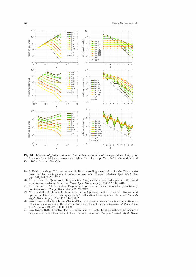
46 Paola Gervasio et al.
10-3
10-2
10-1
100
101
h
10-4
10-3
10-2
10-1
100
101
min
imu
m e
ige
nva
lue
p=2
p=3
p=4
p=5
p=6
p=7
p=8
p=9
p=10
h
h-1
h-2
2 3 4 5 6 7 8 9 10
p
10-4
10-3
10-2
10-1
100
101
min
imum
eig
envalu
e
h=1/4
h=1/8
h=1/16
h=1/32
h=1/64
h=1/128
h=1/256
h=1/512
e-p
3.3-p
10-3
10-2
10-1
100
101
h
10-5
10-4
10-3
10-2
10-1
100
min
imu
m e
ige
nva
lue
p=2
p=3
p=4
p=5
p=6
p=7
p=8
p=9
p=10
h
h-1
2 3 4 5 6 7 8 9 10
p
10-5
10-4
10-3
10-2
10-1
100
min
imum
eig
envalu
eh=1/4
h=1/8
h=1/16
h=1/32
h=1/64
h=1/128
h=1/256
h=1/512
e-p
3-p
10-3
10-2
10-1
100
101
h
10-8
10-6
10-4
10-2
100
min
imu
m e
ige
nva
lue
p=2
p=3
p=4
p=5
p=6
p=7
p=8
p=9
p=10
h
h-1
2 3 4 5 6 7 8 9 10
p
10-8
10-6
10-4
10-2
100
min
imu
m e
ige
nva
lue
h=1/4
h=1/8
h=1/16
h=1/32
h=1/64
h=1/128
h=1/256
h=1/512
e-p
2.3-p
Fig. 37 Advection-diffusion test case. The minimum modulus of the eigenvalues of Ap−1 ford = 1, versus h (at left) and versus p (at right). Pe = 1 at top, Pe = 102 in the middle, andPe = 104 at bottom. See (52)
19. L. Beirao da Veiga, C. Lovadina, and A. Reali. Avoiding shear locking for the Timoshenkobeam problem via isogeometric collocation methods. Comput. Methods Appl. Mech. En-grg., 241/244:38–51, 2012.
20. L. Dede and A. Quarteroni. Isogeometric Analysis for second order partial differentialequations on surfaces. Comp. Methods Appl. Mech. Engrg., 284:807–834, 2015.
21. L. Dede and H.A.F.A. Santos. B-spline goal–oriented error estimators for geometricallynonlinear rods. Comp. Mech., 49(1):35–52, 2012.
22. M. Donatelli, C. Garoni, C. Manni, S. Serra-Capizzano, and H. Speleers. Robust andoptimal multi-iterative techniques for IgA collocation linear systems. Comput. MethodsAppl. Mech. Engrg., 284:1120–1146, 2015.
23. J.A. Evans, Y. Bazilevs, I. Babuska, and T.J.R. Hughes. n–widths, sup–infs, and optimalityratios for the k–version of the Isogeometric finite element method. Comput. Methods Appl.Mech. Engrg., 198:1726–1741, 2009.
24. J.A. Evans, R.R. Hiemstra, T.J.R. Hughes, and A. Reali. Explicit higher-order accurateisogeometric collocation methods for structural dynamics. Comput. Methods Appl. Mech.
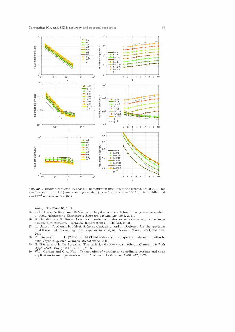
Comparing IGA and SEM: accuracy and spectral properties 47
10-3
10-2
10-1
100
101
h
100
101
102
103
104
ma
xim
um
eig
en
va
lue
p=2
p=3
p=4
p=5
p=6
p=7
p=8
p=9
p=10
h-1
2 3 4 5 6 7 8 9 10
p
100
101
102
103
104
ma
xim
um
eig
en
va
lue
h=1/4
h=1/8
h=1/16
h=1/32
h=1/64
h=1/128
h=1/256
h=1/512
p
10-2
100
h
10-1
100
101
102
maxim
um
eig
envalu
e
p=2
p=3
p=4
p=5
p=6
p=7
p=8
p=9
p=10
h-1
2 3 4 5 6 7 8 9 10
p
10-1
100
101
102
maxim
um
eig
envalu
eh=1/4
h=1/8
h=1/16
h=1/32
h=1/64
h=1/128
h=1/256
h=1/512
p
p-1/2
10-3
10-2
10-1
100
101
h
10-1
100
101
ma
xim
um
eig
en
va
lue
p=2
p=3
p=4
p=5
p=6
p=7
p=8
p=9
p=10
2 3 4 5 6 7 8 9 10
p
0.4
0.5
0.6
0.7
0.8
ma
xim
um
eig
en
va
lue
h=1/4
h=1/8
h=1/16
h=1/32
h=1/64
h=1/128
h=1/256
h=1/512
p-1/2
Fig. 38 Advection-diffusion test case. The maximum modulus of the eigenvalues of Ap−1 ford = 1, versus h (at left) and versus p (at right). ν = 1 at top, ν = 10−2 in the middle, andν = 10−4 at bottom. See (51)
Engrg., 338:208–240, 2018.25. C. De Falco, A. Reali, and R. Vazquez. Geopdes: A research tool for isogeometric analysis
of pdes. Advances in Engineering Software, 42(12):1020–1034, 2011.26. K. Gahalaut and S. Tomar. Condition number estimates for matrices arising in the isoge-
ometric discretizations. Technical Report 2012-23, RICAM, 2012.27. C. Garoni, C. Manni, F. Pelosi, S. Serra Capizzano, and H. Speleers. On the spectrum
of stiffness matrices arising from isogeometric analysis. Numer. Math., 127(4):751–799,2014.
28. P. Gervasio. CHQZ lib: a MATLAB c©library for spectral element methods.http://paola-gervasio.unibs.it/software, 2007.
29. H. Gomez and L. De Lorenzis. The variational collocation method. Comput. MethodsAppl. Mech. Engrg., 309:152–181, 2016.
30. W.J. Gordon and C.A. Hall. Construction of curvilinear co-ordinate systems and theirapplication to mesh generation. Int. J. Numer. Meth. Eng., 7:461–477, 1973.
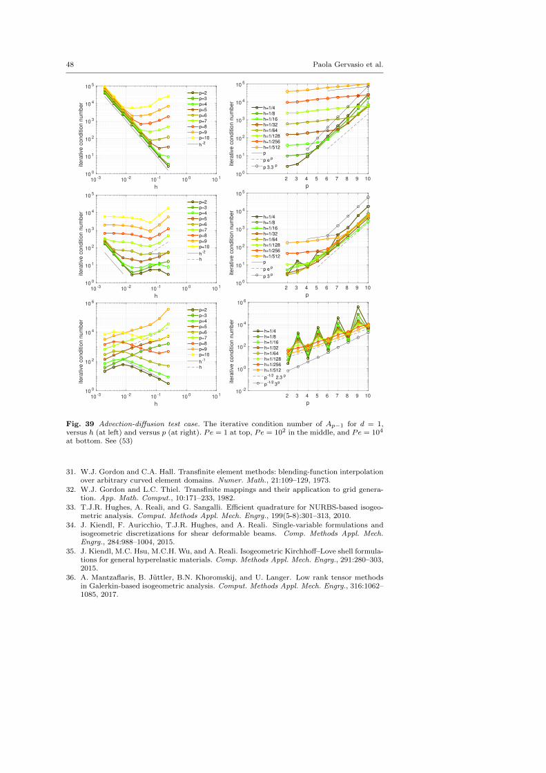
48 Paola Gervasio et al.
10-3
10-2
10-1
100
101
h
100
101
102
103
104
105
ite
rative
co
nd
itio
n n
um
be
r
p=2
p=3
p=4
p=5
p=6
p=7
p=8
p=9
p=10
h-2
2 3 4 5 6 7 8 9 10
p
100
101
102
103
104
105
ite
rative
co
nd
itio
n n
um
be
r
h=1/4
h=1/8
h=1/16
h=1/32
h=1/64
h=1/128
h=1/256
h=1/512
p
p ep
p 3.3p
10-3
10-2
10-1
100
101
h
100
101
102
103
104
105
ite
rative
co
nd
itio
n n
um
be
r
p=2
p=3
p=4
p=5
p=6
p=7
p=8
p=9
p=10
h-2
h
2 3 4 5 6 7 8 9 10
p
100
101
102
103
104
105
ite
rative
co
nd
itio
n n
um
be
r
h=1/4
h=1/8
h=1/16
h=1/32
h=1/64
h=1/128
h=1/256
h=1/512
p
p ep
p 3p
10-3
10-2
10-1
100
101
h
100
102
104
106
ite
rative
co
nd
itio
n n
um
be
r
p=2
p=3
p=4
p=5
p=6
p=7
p=8
p=9
p=10
h-1
h
2 3 4 5 6 7 8 9 10
p
10-2
100
102
104
106
itera
tive c
onditio
n n
um
ber
h=1/4
h=1/8
h=1/16
h=1/32
h=1/64
h=1/128
h=1/256
h=1/512
p-1/2
2.3p
p-1/2
3p
Fig. 39 Advection-diffusion test case. The iterative condition number of Ap−1 for d = 1,versus h (at left) and versus p (at right). Pe = 1 at top, Pe = 102 in the middle, and Pe = 104
at bottom. See (53)
31. W.J. Gordon and C.A. Hall. Transfinite element methods: blending-function interpolationover arbitrary curved element domains. Numer. Math., 21:109–129, 1973.
32. W.J. Gordon and L.C. Thiel. Transfinite mappings and their application to grid genera-tion. App. Math. Comput., 10:171–233, 1982.
33. T.J.R. Hughes, A. Reali, and G. Sangalli. Efficient quadrature for NURBS-based isogeo-metric analysis. Comput. Methods Appl. Mech. Engrg., 199(5-8):301–313, 2010.
34. J. Kiendl, F. Auricchio, T.J.R. Hughes, and A. Reali. Single-variable formulations andisogeometric discretizations for shear deformable beams. Comp. Methods Appl. Mech.Engrg., 284:988–1004, 2015.
35. J. Kiendl, M.C. Hsu, M.C.H. Wu, and A. Reali. Isogeometric Kirchhoff–Love shell formula-tions for general hyperelastic materials. Comp. Methods Appl. Mech. Engrg., 291:280–303,2015.
36. A. Mantzaflaris, B. Juttler, B.N. Khoromskij, and U. Langer. Low rank tensor methodsin Galerkin-based isogeometric analysis. Comput. Methods Appl. Mech. Engrg., 316:1062–1085, 2017.
Comparing IGA and SEM: accuracy and spectral properties 49
37. F. Maurin, L. Dede, and A. Spadoni. Isogeometric rotation–free analysis of planarextensible–elastica for static and dynamic applications. Nonlinear Dyn., 81(1–2):77–96,2015.
38. J.M. Melenk. On condition numbers in hp-FEM with Gauss-Lobatto-based shape func-tions. J. Comput. Appl. Math., 139(1):21–48, 2002.
39. M. Montardini, G. Sangalli, and L. Tamellini. Optimal-order isogeometric collocation atGalerkin superconvergent points. Comput. Methods Appl. Mech. Engrg., 316:741–757,2017.
40. L.H. Nguyen and D. Schillinger. A collocated isogeometric finite element method basedon Gauss-Lobatto Lagrange extraction of splines. Comput. Methods Appl. Mech. Engrg.,316:720–740, 2017.
41. A. Quarteroni and A. Valli. Numerical Approximation of Partial Differential Equations.Springer Verlag, Heidelberg, 1994.
42. A. Reali and T.J.R. Hughes. An Introduction to Isogeometric Collocation Methods, vol-ume 561 of CISM International Centre for Mechanical Sciences, Courses and Lectures.Springer, Vienna, 2015.
43. G. Sangalli and M. Tani. Matrix-free weighted quadrature for a computationally efficientisogeometric k-method. Comput. Methods Appl. Mech. Engrg., 338:117–133, 2018.
44. D. Schillinger, J.A. Evans, A. Reali, M.A. Scott, and T.J.R. Hughes. Isogeometric col-location: cost comparison with Galerkin methods and extension to adaptive hierarchicalNURBS discretizations. Comput. Methods Appl. Mech. Engrg., 267:170–232, 2013.
45. D. Schillinger, S.J. Hossain, and T.J.R. Hughes. Reduced Bezier element quadrature rulesfor quadratic and cubic splines in isogeometric analysis. Comput. Methods Appl. Mech.Engrg., 277:1–45, 2014.
46. F. Scholz, A. Mantzaflaris, and B. Juttler. Partial tensor decomposition for decouplingisogeometric Galerkin discretizations. Comput. Methods Appl. Mech. Engrg., 336:485–506,2018.
47. A. Tagliabue, L. Dede, and A. Quarteroni. Isogeometric analysis and error estimates forhigh order partial differential equations in fluid dynamics. Comput. Fluids, 102:277–303,2014.
48. H.A. van der Vorst. Iterative Krylov methods for large linear systems. Cambridge Uni-versity Press, Cambridge, 2003.
49. R. Vazquez. A new design for the implementation of isogeometric analysis in octave andmatlab: Geopdes 3.0. Comput. Math. Appl., 72(3):523–554, 2016.
Related Documents


