A Comprehensive Review of Swarm Optimization Algorithms

RESEARCH ARTICLE

A Comprehensive Review of SwarmOptimization AlgorithmsMohd Nadhir AbWahab1☯*, Samia Nefti-Meziani1☯, AdhamAtyabi1,2☯

1 Autonomous System and Advanced Robotics Lab, School of Computing, Science and Engineering,University of Salford, Salford, United Kingdom, 2 School of Computer Science, Engineering andMathematics, Flinders University of South Australia, Adelaide, Australia

☯ These authors contributed equally to this work.* [email protected]

AbstractMany swarm optimization algorithms have been introduced since the early 60’s, Evolution-

ary Programming to the most recent, Grey Wolf Optimization. All of these algorithms have

demonstrated their potential to solve many optimization problems. This paper provides an

in-depth survey of well-known optimization algorithms. Selected algorithms are briefly ex-

plained and compared with each other comprehensively through experiments conducted

using thirty well-known benchmark functions. Their advantages and disadvantages are also

discussed. A number of statistical tests are then carried out to determine the significant per-

formances. The results indicate the overall advantage of Differential Evolution (DE) and is

closely followed by Particle Swarm Optimization (PSO), compared with other considered

approaches.

IntroductionSwarm Intelligence (SI) has attracted interest from many researchers in various fields. Bona-beau defined SI as “The emergent collective intelligence of groups of simple agents” [1]. SI is thecollective intelligence behaviour of self-organized and decentralized systems, e.g., artificialgroups of simple agents. Examples of SI include the group foraging of social insects, coopera-tive transportation, nest-building of social insects, and collective sorting and clustering. Twofundamental concepts that are considered as necessary properties of SI are self-organizationand division of labour. Self-organization is defined as the capability of a system to evolve itsagents or components in to a suitable form without any external help. Bonabeau et al. [1] alsostated that self-organization relies on four fundamental properties of positive feedback, nega-tive feedback, fluctuations and multiple interactions. Positive and negative feedbacks are usefulfor amplification and stabilization respectively. Fluctuations meanwhile are useful for random-ness. Multiple interactions occur when the swarms share information among themselves with-in their searching area. The second property of SI is division of labour which is defined as thesimultaneous execution of various simple and feasible tasks by individuals. This division allowsthe swarm to tackle complex problems that require individuals to work together [1].

PLOSONE | DOI:10.1371/journal.pone.0122827 May 18, 2015 1 / 36

OPEN ACCESS

Citation: Ab Wahab MN, Nefti-Meziani S, Atyabi A(2015) A Comprehensive Review of SwarmOptimization Algorithms. PLoS ONE 10(5):e0122827. doi:10.1371/journal.pone.0122827

Academic Editor: Catalin Buiu, PolitehnicaUniversity of Bucharest, ROMANIA

Received: September 9, 2014

Accepted: February 15, 2015

Published: May 18, 2015

Copyright: © 2015 Ab Wahab et al. This is an openaccess article distributed under the terms of theCreative Commons Attribution License, which permitsunrestricted use, distribution, and reproduction in anymedium, provided the original author and source arecredited.

Data Availability Statement: All relevant data arewithin the paper and its Supporting Information files.

Funding: This research paper was supported by theGAMMA Programme which is funded through theRegional Growth Fund. The Regional Growth Fund(RGF) is a $3.2 billion fund supporting projects andprogrammes which are using private sectorinvestment to generate economic growth as well ascreating sustainable jobs between now and the mid-2020s. For more information, please go to www.bis.gov.uk/rgf. The funders had no role in study design,data collection and analysis, decision to publish, orpreparation of the manuscript.

http://crossmark.crossref.org/dialog/?doi=10.1371/journal.pone.0122827&domain=pdf

http://creativecommons.org/licenses/by/4.0/

http://www.bis.gov.uk/rgf

http://www.bis.gov.uk/rgf

This paper outline starts with brief discussion on seven SI-based algorithms and is followedby general discussion on others available algorithms. After that, an experiment is conducted tomeasure the performance of the considered algorithms on thirty benchmark functions. The re-sults are discussed comprehensively after that with statistical analysis in the following section.From there, the two best performing algorithms are selected to investigate their variants perfor-mance against the best performing algorithm in five benchmark functions. The conclusion sec-tion is presented at the end of this paper.

Swarm Intelligence AlgorithmsThis section introduces several SI-based algorithms, highlighting their notable variants, theirmerits and demerits, and their applications. These algorithms include Genetic Algorithms(GA), Ant Colony Optimization (ACO), Particle Swarm Optimization (PSO), Differential Evo-lution (DE), Artificial Bee Colony (ABC), Glowworm Swarm Optimization (GSO), and Cuck-oo Search Algorithm (CSA).

Genetic AlgorithmThe Genetic Algorithm (GA) introduced by John Holland in 1975 [2, 3], is a search optimiza-tion algorithm based on the mechanics of the natural selection process. The basic concept ofthis algorithm is to mimic the concept of the ‘survival of the fittest’; it simulates the processesobserved in a natural system where the strong tends to adapt and survive while the weak tendsto perish. GA is a population based approach in which members of the population are rankedbased on their solutions’ fitness. In GA, a new population is formed using specific genetic oper-ators such as crossover, reproduction, and mutation [4–7]. Population can be represented in aset of strings (referred to as chromosomes). In each generation, a new chromosome (a memberof the population) is created using information originated from the fittest chromosomes of theprevious population [4–6]. GA generates an initial population of feasible solutions and recom-bines them in a way to guide their search toward more promising areas of the search space.Each of these feasible solutions is encoded as a chromosome, also referred to as genotype, andeach of these chromosomes will get a measure of fitness through a fitness function (evaluationor objective function). The value of fitness function of a chromosome determines its capabilityto endure and produce offspring. The high fitness value indicates the better solution for maxi-mization and the low fitness value shows the better solution for minimization problems. Abasic GA has five main components: a random number generator, a fitness evaluation unit, areproduction process, a crossover process, and a mutation operation. Reproduction selects thefittest candidates of the population, while crossover is the procedure of combining the fittestchromosomes and passing superior genes to the next generation, and mutation alters some ofthe genes in a chromosome [4–7].

Fig 1 shows the general flow chart of GA and the main components that contribute to theoverall algorithm. The operation of the GA starts with determining an initial populationwhether randomly or by the use of some heuristics. The fitness function is used to evaluate themembers of the population and then they are ranked based on the performances. Once all themembers of the population have been evaluated, the lower rank chromosomes are omitted andthe remaining populations are used for reproduction. This is one of the most common ap-proaches used for GA. Another possible selection scheme is to use pseudo-random selection,allowing lower rank chromosomes to have a chance to be selected for reproduction. The cross-over step randomly selects two members of the remaining population (the fittest chromo-somes) and exchanges and mates them. The final step of GA is mutation. In this step, themutation operator randomly mutates on a gene of a chromosome. Mutation is a crucial step in

Swarm Optimization Algorithms: A Survey

PLOS ONE | DOI:10.1371/journal.pone.0122827 May 18, 2015 2 / 36

Competing Interests: The authors have declaredthat no competing interests exist.

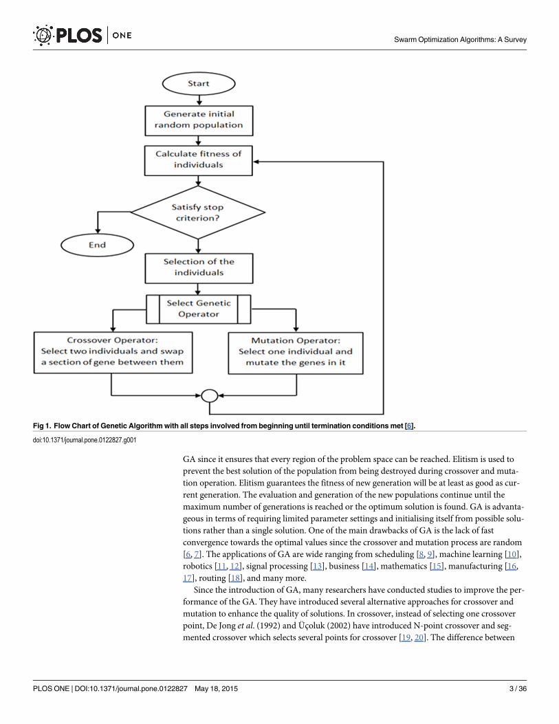
GA since it ensures that every region of the problem space can be reached. Elitism is used toprevent the best solution of the population from being destroyed during crossover and muta-tion operation. Elitism guarantees the fitness of new generation will be at least as good as cur-rent generation. The evaluation and generation of the new populations continue until themaximum number of generations is reached or the optimum solution is found. GA is advanta-geous in terms of requiring limited parameter settings and initialising itself from possible solu-tions rather than a single solution. One of the main drawbacks of GA is the lack of fastconvergence towards the optimal values since the crossover and mutation process are random[6, 7]. The applications of GA are wide ranging from scheduling [8, 9], machine learning [10],robotics [11, 12], signal processing [13], business [14], mathematics [15], manufacturing [16,17], routing [18], and many more.

Since the introduction of GA, many researchers have conducted studies to improve the per-formance of the GA. They have introduced several alternative approaches for crossover andmutation to enhance the quality of solutions. In crossover, instead of selecting one crossoverpoint, De Jong et al. (1992) and Üçoluk (2002) have introduced N-point crossover and seg-mented crossover which selects several points for crossover [19, 20]. The difference between

Fig 1. Flow Chart of Genetic Algorithmwith all steps involved from beginning until termination conditions met [6].

doi:10.1371/journal.pone.0122827.g001



them is N-point crossover is choosing several breaking points randomly, while in segmentedcrossover, only two breaking points are utilized. Mutation is one of the most important opera-tors in GA in order to direct the chromosomes towards the better solution. Therefore, severalstudies have given different methods for mutation. By default, each gene in a chromosome isassigned with probability, pm, and mutated depending on that probability. This mutation isknown as uniform mutation. The other approaches for mutation are bitwise inversion wherethe whole gene in a chromosome is mutated using a random mutation [19]. Adaptive geneticalgorithms have been introduced in order to allow the use of precise parameters in setting thepopulation size, the crossing over probability, and the mutation probability. All of these param-eters are dynamic and changing over the iterations. For instance, if the population is not im-proving, the mutation rate is increasing and whenever the population is improving, themutation rate starts decreasing [21]. Raja and Bhaskaran [22] have suggested a new approachof GA initialization that improve the overall performance of GA. In this approach, they utilizedinitialization twice where the first initialization is uses to identify the promising area. After thefirst initialization, all chromosome are ranked and the best chromosomes are selected. Afterthat, GA is initialize again within the area where the best chromosomes have been identified.

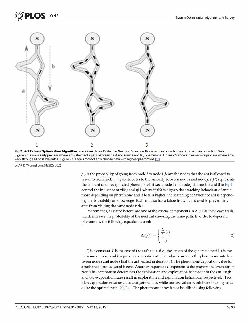
Ant Colony OptimizationAnt Colony Optimization (ACO) is a metaheuristic approach inspired by the Ant System (AS)proposed by Marco Dorigo in 1992 in his PhD thesis [23–25]. It is inspired by the foraging be-haviour of real ants. This algorithm consists of four main components (ant, pheromone, dae-mon action, and decentralized control) that contribute to the overall system. Ants areimaginary agents that are used in order to mimic the exploration and exploitation of the searchspace. In real life pheromone is a chemical material spread by ants over the path they traveland its intensity changes over time due to evaporation. In ACO the ants drop pheromoneswhen traveling in the search space and the quantities of these pheromones indicate the intensi-ty of the trail. The ants choose the direction based on path marked by the high intensity of thetrail. The intensity of the trail can be considered as a global memory of the system. Daemon ac-tions is used to gather global information which cannot be done by a single ant and uses the in-formation to determine whether it is necessary to add extra pheromone in order to help theconvergence. The decentralized control is used in order to make the algorithm robust and flexi-ble within a dynamic environment. The importance of having a decentralized system in ACOis due to resulting flexibility in the face of ant lost or ant failure offered by such a system. Thesebasic components contribute to a cooperative interaction that leads to the emergence of short-est paths [23, 24]. Fig 2.1, 2.2, and 2.3 depict the initial phase, mid-range status of any system,and the final outcomes of the ACO algorithm respectively. The left figure illustrates the initialenvironment when the algorithm starts, where an agent (ant) starts moving randomly from thenest towards the source and returns back. The middle figure illustrates several iterations of exe-cution when ants discover multiple possible paths between nest and source. The shortest pathis chosen, and ants use this path frequently which contributes to high intensity of pheromonetrail as shown in the sub-figure 3 in Fig 2. N, S, a, and b represent nest, food source, on-goingpath, and returning path respectively. The steps involved to find the best solution starts withchoosing the next node (from the current position in the search space) using following equa-tion:

pkði;jÞðtÞ ¼ð½tijðtÞ�a � ½Zij�bÞ

ðXk2Jk

½tijðtÞ�a � ½Zij�bÞð1Þ



pi,j is the probability of going from node i to node j. Jk are the nodes that the ant is allowed totravel to from node i. ηi j contributes to the visibility between node i and node j. τij(t) representsthe amount of un-evaporated pheromone between node i and node j at time t. α and β in Eq 1control the influence of τij(t) and ηi j, where if alfa is higher, the searching behaviour of ant ismore depending on pheromone and if beta is higher, the searching behaviour of ant is depend-ing on its visibility or knowledge. Each ant also has a taboo list which is used to prevent anyants from visiting the same node twice.

Pheromones, as stated before, are one of the crucial components in ACO as they leave trailswhich increase the probability of the next ant choosing the same path. In order to deposit apheromone, the following equation is used:

DtkijðtÞ ¼QLk

ðtÞ

0

ð2Þ8<:

Q is a constant, L is the cost of the ant's tour, (i.e., the length of the generated path), t is theiteration number and k represents a specific ant. The value represents the pheromone rate be-tween node i and node j that the ant visited in iteration t. The pheromone deposition value fora path that is not selected is zero. Another important component is the pheromone evaporationrate. This component determines the exploration and exploitation behaviour of the ant. Highand low evaporation rates result in exploration and exploitation behaviours respectively. Toohigh exploration rates result in ants getting lost, while too low values result in an inability to ac-quire the optimal path [23, 24]. The pheromone decay factor is utilized using following

Fig 2. Ant Colony Optimization Algorithm processes. N and S denote Nest and Source with a is ongoing direction and b is returning direction. SubFigure 2.1 shows early process where ants start find a path between nest and source and lay pheromone. Figure 2.2 shows intermediate process where antswent through all possible paths. Figure 2.3 shows most of ants choose path with highest pheromone [18].




equation:

tði;jÞðt þ 1Þ ¼ ð1� pÞ � tði;jÞðtÞ þXm

ðk¼1Þ½Dtkði;jÞðtÞ� ð3Þ

m is the number of ants in the system and p is the pheromone evaporation rate or decay factor.ACO has several advantages over other evolutionary approaches including offering positivefeedback resulting in rapid solution finding, and having distributed computation which avoidspremature convergence. These are in addition to taking advantage of the existing collective in-teraction of a population of agents [26, 27]. However, ACO has drawbacks such as slower con-vergence compared with other heuristic-based methods and lack a centralized processor toguide it towards good solutions. Although the convergence is guaranteed, the time for conver-gence is uncertain. Another important demerit of ACO is its poor performance within prob-lems with large search spaces [26, 27]. ACO has been applied in various optimization problemssuch as traveling salesman problem (TSP) [28], quadratic assignment problem [29], vehiclerouting [30], network model problem [31, 32], image processing [33], path planning for mobilerobot [34], path optimization for UAV System [35], project management [36] and so on.

A number of ACO variants have been created with the aim to improve overall performance.Two years after the introduction of ACO, Dorigo and Gambardella made modifications by im-proving three major aspects (pheromone, state transition rule and local search procedures)which produce the variant of ACO called Ant Colony System (ACS) [37]. GA is initialize again

ACS uses centralise (global) update approach for pheromone update and only concentratethe search within a neighbourhood of the best solution found so far in order to increase effi-ciency for convergence time. The state transition rule is different from ACO where ACS has astated probability (q0) to decide which behaviour is used by the ant. q0 is usually set to 0.9 andcompare to a value of q (which 0� q� 1). If the value of q is less than that, then exploitationbehaviour is used and vice versa. For local search procedures, a local optimization heuristicbased on an edge exchange strategy such as 2-opt, 3-opt or Lin-Kernighan is applied to each so-lution generated by an ant to get its local minima. This combination of new pheromone man-agement, new state transition, and local search procedures has produced a variant of ACO forTSP problems [37]. Max-Min Ant System (MMAS) is considered as another notable variant ofACO. The approach was introduced by Stutzle and Hoos in 2000 and it limits the pheromonetrail values within the interval of [τmin, τmax] [38]. MMAS also modified three aspects of ACO.First, at the beginning, the pheromone trails are set to the maximum value which escalate theexploration behaviour of the ants. Second, the authors introduce an interval of [τmin, τmax]which limits the pheromone trails in order to avoid stagnation. Third, only one ant is allowedto add pheromone which help exploiting the best solutions found during the execution of thealgorithm. The pheromone may be added by using either an iteration-best approach or a glob-al-best approach. In the iteration-best approach, only the ant with best solution adds the phero-mone for each iteration while in the global-best approach, the ant with the best solution canadd the pheromone without considering other ants in the same iteration [38].

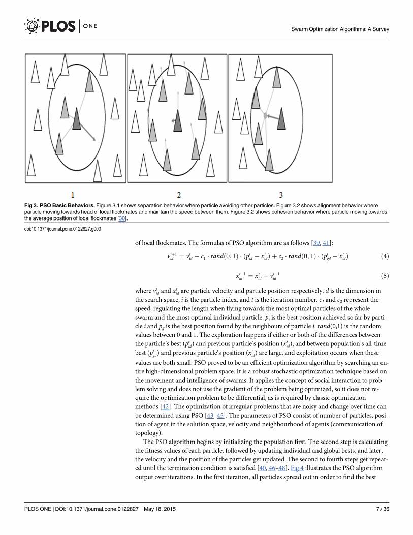
Particle Swarm OptimizationParticle Swarm Optimization (PSO) is an optimization technique introduced by Kennedy andEberhart in 1995 [39]. It uses a simple mechanism that mimics swarm behaviour in birds flock-ing and fish schooling to guide the particles to search for global optimal solutions. Del Valleand his co-authors [40] described PSO with three simple behaviours of separation, alignment,and cohesion as shown in Fig 3 respectively. Separation is the behaviour of avoiding thecrowded local flockmates while alignment is the behaviour of moving towards the average di-rection of local flockmates. Cohesion is the behaviour of moving towards the average position



of local flockmates. The formulas of PSO algorithm are as follows [39, 41]:

vtþ1id ¼ vtid þ c1 � randð0; 1Þ � ðptid � xtidÞ þ c2 � randð0; 1Þ � ðptgd � xtidÞ ð4Þ

xtþ1id ¼ xtid þ vtþ1

id ð5Þ

where vtid and xtid are particle velocity and particle position respectively. d is the dimension in

the search space, i is the particle index, and t is the iteration number. c1 and c2 represent thespeed, regulating the length when flying towards the most optimal particles of the wholeswarm and the most optimal individual particle. pi is the best position achieved so far by parti-cle i and pg is the best position found by the neighbours of particle i. rand(0,1) is the randomvalues between 0 and 1. The exploration happens if either or both of the differences betweenthe particle’s best (ptid) and previous particle’s position (xtid), and between population’s all-timebest (ptgd) and previous particle’s position (xtid) are large, and exploitation occurs when these

values are both small. PSO proved to be an efficient optimization algorithm by searching an en-tire high-dimensional problem space. It is a robust stochastic optimization technique based onthe movement and intelligence of swarms. It applies the concept of social interaction to prob-lem solving and does not use the gradient of the problem being optimized, so it does not re-quire the optimization problem to be differential, as is required by classic optimizationmethods [42]. The optimization of irregular problems that are noisy and change over time canbe determined using PSO [43–45]. The parameters of PSO consist of number of particles, posi-tion of agent in the solution space, velocity and neighbourhood of agents (communication oftopology).

The PSO algorithm begins by initializing the population first. The second step is calculatingthe fitness values of each particle, followed by updating individual and global bests, and later,the velocity and the position of the particles get updated. The second to fourth steps get repeat-ed until the termination condition is satisfied [40, 46–48]. Fig 4 illustrates the PSO algorithmoutput over iterations. In the first iteration, all particles spread out in order to find the best

Fig 3. PSO Basic Behaviors. Figure 3.1 shows separation behavior where particle avoiding other particles. Figure 3.2 shows alignment behavior whereparticle moving towards head of local flockmates and maintain the speed between them. Figure 3.2 shows cohesion behavior where particle moving towardsthe average position of local flockmates [30].




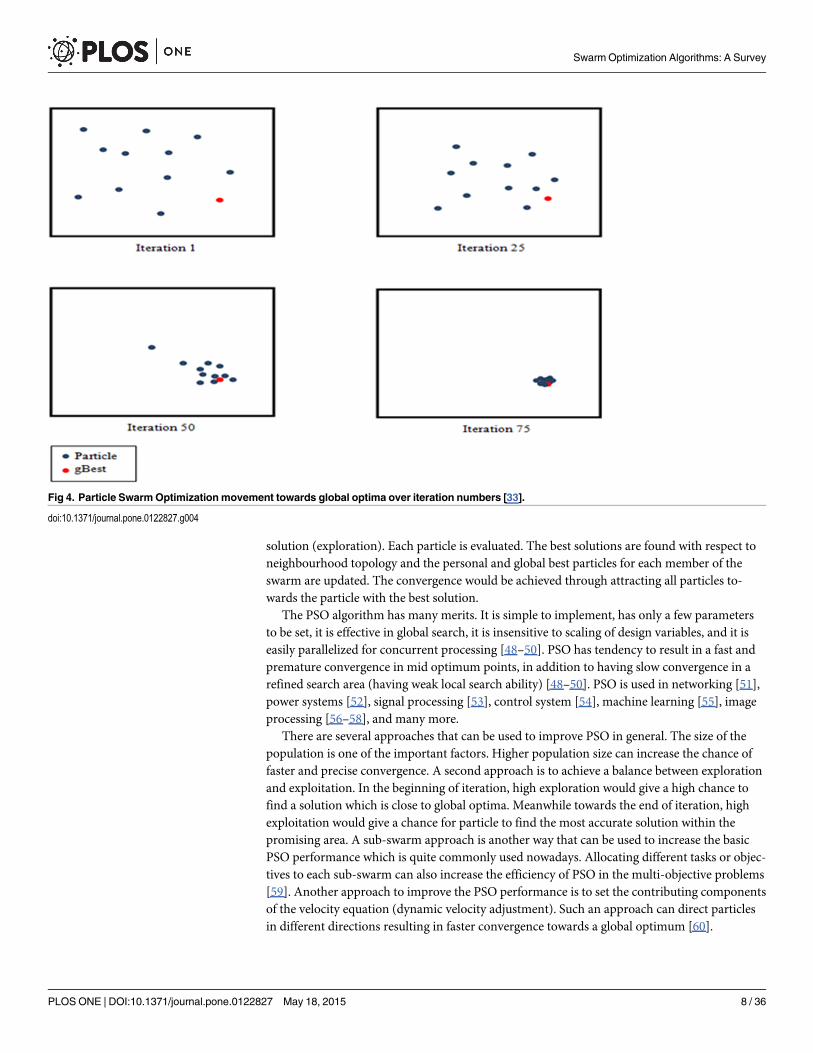
solution (exploration). Each particle is evaluated. The best solutions are found with respect toneighbourhood topology and the personal and global best particles for each member of theswarm are updated. The convergence would be achieved through attracting all particles to-wards the particle with the best solution.

The PSO algorithm has many merits. It is simple to implement, has only a few parametersto be set, it is effective in global search, it is insensitive to scaling of design variables, and it iseasily parallelized for concurrent processing [48–50]. PSO has tendency to result in a fast andpremature convergence in mid optimum points, in addition to having slow convergence in arefined search area (having weak local search ability) [48–50]. PSO is used in networking [51],power systems [52], signal processing [53], control system [54], machine learning [55], imageprocessing [56–58], and many more.

There are several approaches that can be used to improve PSO in general. The size of thepopulation is one of the important factors. Higher population size can increase the chance offaster and precise convergence. A second approach is to achieve a balance between explorationand exploitation. In the beginning of iteration, high exploration would give a high chance tofind a solution which is close to global optima. Meanwhile towards the end of iteration, highexploitation would give a chance for particle to find the most accurate solution within thepromising area. A sub-swarm approach is another way that can be used to increase the basicPSO performance which is quite commonly used nowadays. Allocating different tasks or objec-tives to each sub-swarm can also increase the efficiency of PSO in the multi-objective problems[59]. Another approach to improve the PSO performance is to set the contributing componentsof the velocity equation (dynamic velocity adjustment). Such an approach can direct particlesin different directions resulting in faster convergence towards a global optimum [60].

Fig 4. Particle SwarmOptimization movement towards global optima over iteration numbers [33].




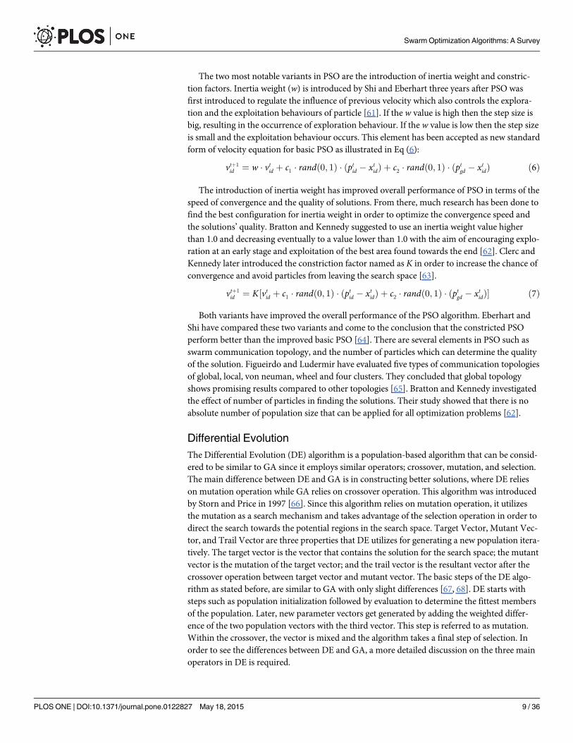
The two most notable variants in PSO are the introduction of inertia weight and constric-tion factors. Inertia weight (w) is introduced by Shi and Eberhart three years after PSO wasfirst introduced to regulate the influence of previous velocity which also controls the explora-tion and the exploitation behaviours of particle [61]. If the w value is high then the step size isbig, resulting in the occurrence of exploration behaviour. If the w value is low then the step sizeis small and the exploitation behaviour occurs. This element has been accepted as new standardform of velocity equation for basic PSO as illustrated in Eq (6):

vtþ1id ¼ w � vtid þ c1 � randð0; 1Þ � ðptid � xtidÞ þ c2 � randð0; 1Þ � ðptgd � xtidÞ ð6Þ

The introduction of inertia weight has improved overall performance of PSO in terms of thespeed of convergence and the quality of solutions. From there, much research has been done tofind the best configuration for inertia weight in order to optimize the convergence speed andthe solutions’ quality. Bratton and Kennedy suggested to use an inertia weight value higherthan 1.0 and decreasing eventually to a value lower than 1.0 with the aim of encouraging explo-ration at an early stage and exploitation of the best area found towards the end [62]. Clerc andKennedy later introduced the constriction factor named as K in order to increase the chance ofconvergence and avoid particles from leaving the search space [63].

vtþ1id ¼ K½vtid þ c1 � randð0; 1Þ � ðptid � xtidÞ þ c2 � randð0; 1Þ � ðptgd � xtidÞ� ð7Þ

Both variants have improved the overall performance of the PSO algorithm. Eberhart andShi have compared these two variants and come to the conclusion that the constricted PSOperform better than the improved basic PSO [64]. There are several elements in PSO such asswarm communication topology, and the number of particles which can determine the qualityof the solution. Figueirdo and Ludermir have evaluated five types of communication topologiesof global, local, von neuman, wheel and four clusters. They concluded that global topologyshows promising results compared to other topologies [65]. Bratton and Kennedy investigatedthe effect of number of particles in finding the solutions. Their study showed that there is noabsolute number of population size that can be applied for all optimization problems [62].

Differential EvolutionThe Differential Evolution (DE) algorithm is a population-based algorithm that can be consid-ered to be similar to GA since it employs similar operators; crossover, mutation, and selection.The main difference between DE and GA is in constructing better solutions, where DE relieson mutation operation while GA relies on crossover operation. This algorithm was introducedby Storn and Price in 1997 [66]. Since this algorithm relies on mutation operation, it utilizesthe mutation as a search mechanism and takes advantage of the selection operation in order todirect the search towards the potential regions in the search space. Target Vector, Mutant Vec-tor, and Trail Vector are three properties that DE utilizes for generating a new population itera-tively. The target vector is the vector that contains the solution for the search space; the mutantvector is the mutation of the target vector; and the trail vector is the resultant vector after thecrossover operation between target vector and mutant vector. The basic steps of the DE algo-rithm as stated before, are similar to GA with only slight differences [67, 68]. DE starts withsteps such as population initialization followed by evaluation to determine the fittest membersof the population. Later, new parameter vectors get generated by adding the weighted differ-ence of the two population vectors with the third vector. This step is referred to as mutation.Within the crossover, the vector is mixed and the algorithm takes a final step of selection. Inorder to see the differences between DE and GA, a more detailed discussion on the three mainoperators in DE is required.



In the mutation step each of N parameter vectors goes through mutation. Mutation is theoperation of expanding the search space and a mutant vector is generated by:

vi;Gþ1 ¼ xr1;G þ Fðxr2;G � xr3;GÞ ð8Þ

where F is the scaling factor with a value in the range of [0,1] with solution vectors xr1, xr2, andxr3 being chosen randomly and satisfying following criteria:

xr1; xr2; xr3jr1 6¼ r2 6¼ r3 6¼ i ð9Þ

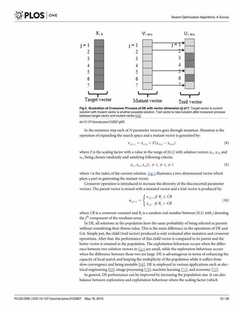
where i is the index of the current solution. Fig 5 illustrates a two-dimensional vector whichplays a part in generating the mutant vector.

Crossover operation is introduced to increase the diversity of the disconcerted parametervectors. The parent vector is mixed with a mutated vector and a trial vector is produced by:

ui;Gþ1 ¼vi;Gþ1 if Rj � CR

xi;G if Rj > CRð10Þ

(

where CR is a crossover constant and Rj is a random real number between [0,1] with j denotingthe jth component of the resultant array.

In DE, all solutions in the population have the same probability of being selected as parentswithout considering their fitness value. This is the main difference in the operations of DE andGA. Simply put, the child (trail vector) produced is only evaluated after mutation and crossoveroperations. After that, the performance of this child vector is compared to its parent and thebetter vector is retained in the population. The exploitation behaviour occurs when the differ-ence between two solution vectors in Eq 6 are small, while the exploration behaviour occurswhen the difference between those two are large. DE is advantageous in terms of enhancing thecapacity of local search and keeping the multiplicity of the population while it suffers fromslow convergence and being unstable [68]. DE is employed in various applications such as elec-trical engineering [69], image processing [70], machine learning [71], and economy [72].

In general, DE performance can be improved by increasing the population size. It can alsobalance between exploration and exploitation behaviour where the scaling factor (which

Fig 5. Illustration of Crossover Process of DE with vector dimension (j) of 7. Target vector is currentsolution with mutant vector is another possible solution. Trail vector is new solution after crossover processbetween target vector and mutant vector [43].




determines the step size) is high at the beginning and decreases towards the end of an iteration.Another step that can be used is the introduction of elitism which can avoid the best solutionfrom being destroyed when the next generation is created. There are many variants of DE avail-able since its introduction by Storn and Price. Mezura-Montes et al. have discussed several var-iants of DE and done a comparative study between them [73]. The variants discussed are DE/rand/1/bin, DE/rand/1/exp, DE/best/1/bin, DE/best/1/exp, DE/current-to-best/1, DE/current-to-rand/1, DE/current-to-rand/1/bin, and DE/rand/2/dir. The differences between them are interms of individuals selected for mutation, the numbers of pairs of solutions selected and thetype of recombination [74]. In the study the variants of DE are described in DE/x/y/z formwhere x represents a string denoting the base vector to be perturbed; for example randmeansthat vectors selected randomly to produce the mutation values and bestmeans that the bestvectors among population is selected to produce the mutation values. y is the number of vectorsconsidered to generate a new vector and is represented in an integer form which indicate thenumber of pairs of solutions used to produce a new solution. z represents the type of crossover,for instance bin and exp (binmeaning binomial and expmeaning exponential). Meanwhile,current-to-best and current-to-rand are arithmetic recombination proposed by Price [75] toeliminate the binomial and exponential crossover operator with the rotation invariant.

Artificial Bee ColonyArtificial Bee Colony (ABC) is one of the most recent swarm intelligence algorithms. It wasproposed by Dervis Karaboga in 2005 [76]; in 2007, the performance of ABC was analysed [77]and it was concluded that ABC performs quite well compared with several other approaches.This algorithm is inspired by the intelligent behaviour of real honey bees in finding foodsources, known as nectar, and the sharing of information about that food source among otherbees in the nest. This algorithm is claimed to be as simple and easy to implement as PSO andDE [78]. In this approach, the artificial agents are defined and categorized into three types, theemployed bee, the onlooker bee, and the scout bee. Each of these bees has different tasks as-signed to them in order to complete the algorithm’s process. The employed bees focus on afood source and retain the locality of that food source in their memories. The number of em-ployed bees is equal to the number of food sources since each employed bee is associated withone and only one food source. The onlooker bee receives the information of the food sourcefrom the employed bee in the hive. After that, one of the food sources is selected to gather thenectar. The scout bee is in charge of finding new food sources and the new nectar. The generalprocess of ABC method and the details of each step are as follows [76–78]:

Step 1. Initialization Phase: All the vectors of the population of food source, xl!, are initial-

ized (i = 1. . .SN, where SN is population size) by scout bees and control parameters being set.

Each xl! vector holds n variables, which is optimized, to minimize the objective function. The

following equation is used for initialization phase:

xi ¼ li þ randð0; 1Þ � ðui � liÞ ð11Þwhere li and ui respectively are the lower and upper bound parameters of xi.

Step 2.Employed Bees Phase: In this phase, the search for a new food source, vl!, increases in

order to have more nectar around the neighbourhood of the food source, xl!. Once a neigh-

bouring food source is found, its profitability or fitness is evaluated. The new neighbouringfood source is defined by using following formula:

vi ¼ xi þO=iðxi � xjÞ ð12Þ

where xj is a random selected food source and Øi is a random number of [-a, a]. Once the new



food source, vi, is produced its profitability is measured and a greedy selection is applied be-

tween xl! and vl

!. The exploration happens if the difference between xi − xj is large and the ex-

ploitation behaviour is when the difference is small. The fitness value of the solution, fiti(xl!), is

determined using following equation:

fitið xi!Þ ¼1

1þ fið xi!Þ if fiðxi!Þ � 0

1þ absðfiðxi!ÞÞ if fið xi!Þ < 0

ð13Þ

8><>:

where fi ð xl!Þ is the objective function value of solution (xi!).

Step 3. Onlooker Bees Phase: Onlooker bees that are waiting in the hive choose their foodsources depending on probability values measured using the fitness value and the informationshared by employed bees. The probability value, pi, is measured using the following equation:

pi ¼fitið xi!ÞXSN

i¼1fitið xi!Þ

ð14Þ

Step 4. Scout Bees Phase: The scout bees are those unemployed bees that choose their foodsources randomly. Employed bees whose fitness values cannot be improved through predeter-mined number of iterations, called as limit or abandonment criteria, become the scout bees andall their food sources get abandoned.

Step 5. The best fitness value and the position associated to that value are memorized.Step 6. Termination Checking Phase: If the termination condition is met, the programme

terminates, otherwise the programme returns to Step 2 and repeats until the termination con-dition is met.

Advantages of ABC include being easy to implement, robust, and highly flexible. It is con-sidered as highly flexible since only requires two control parameters of maximum cycle numberand colony size. Therefore, adding and removing bee can be done without need to reinitializethe algorithm. It can be used in many optimization problems without any modification, and itrequires fewer control parameters compared with other search techniques [77–80]. The disad-vantages of ABC include the requirement of new fitness tests for the new parameters to im-prove performance, being quite slow when used in serial processing, and the need for a highamount of objective function evaluations [81]. ABC has been implemented in various fields in-cluding engineering design problems [82, 83], networking [84], business [85], electronics [86],scheduling [86] and image processing [86].

Although ABC algorithm was only been introduced less than ten years ago there are alreadyquite number of variants of ABC available. One of the important ABC variant is InteractiveABC (IABC) designed to solve numerical optimization problems [87]. Bao and Zeng have in-troduced three selection strategies of food source by onlooker bees for ABC which form threevariants called Rank Selection Strategies ABC (RABC), Tournament Selection ABC (TABC)and Disruptive Selection ABC (DABC) [88]. The main aim for all these variants is to upsurgethe population diversity and avoid premature convergence. Bao and Zeng have tested thesemodified ABCs with the standard ABC and the results showed that these three selection strate-gies perform better search compared with the standard ABC [88].

Glowworm Swarm OptimizationGlow worm Swarm Optimization (GSO) is a new SI-based technique aimed to optimize multi-modal functions, proposed by Krishnanad and Ghose in 2005 [89, 90]. GSO employs physicalentities (agents) called glowworms. A condition of glowwormm, at time t has three main



parameters of a position in the search space (xm(t)), a luciferin level (lm(t)) and a neighbour-hood range (rm(t)). These three parameters change over time [89–91]. Initially the glowwormsare distributed randomly in the workspace, instead of finite regions being randomly placed inthe search area as demonstrated in ACO. Later, other parameters are initialized using prede-fined constants. Yet, similar to other methods, three phases are repeated until the terminationcondition is satisfied. These phases are luciferin level update, glowworm movement, and neigh-bourhood range update [89]. In order to update the luciferin level, the fitness of current posi-tion of a glowwormm is determined using following equation:

lmðtÞ ¼ ð1� pÞ � lmðt � 1Þ þ gJðxmðtÞÞ ð15Þ

where p is the luciferin evaporation factor, γ is the luciferin constant and J is an objective func-tion. The position in the search space is updated using following equation:

xmðtÞ ¼ xmðt � 1Þ þ sxnðt � 1Þ � xmðt � 1Þ

k xnðt � 1Þ � xmðt � 1Þ k� �

ð16Þ

where s is the step size, and ||.|| is Euclidean norm operator. If the difference between xn and xmis large then exploration behaviour takes place and if this difference is small then exploitationbehaviour occurs. Later, each glowworm tries to find its neighbours. In GSO, a glowwormm isthe neighbour of glowworm n only if the distance between them is shorter than the neighbour-hood range rm(t), and on condition where glowworm n is brighter than glowwormm. Howev-er, if a glowworm has multiple choices of neighbours, one neighbour is selected using thefollowing probability equation.

pmðtÞ ¼lmðtÞ�lnðtÞXk2NiðtÞlkðtÞ�lnðtÞ

ð17Þ

where the probability of glowworm atmmoving towards glowworm at n is the difference of lu-ciferin level between them over difference of luciferin level between all glowworms within therange of glowwormm. The solution with the highest probability is selected and then the glow-worm moves one step closer in direction of the chosen neighbour with a constant step size s. Inthe final phase, the neighbourhood range (rm(t)) is updated to limit the range of communica-tion in a group of glowworms. The neighbourhood range is calculated using following equa-tion:

rmðt þ 1Þ ¼ min rs;max 0; rmðtÞ þ b nd � jnmðtÞjð Þ½ �f g ð18Þ

where rs is a sensor range (a constant that limits the size of the neighbourhood range), nd is thedesired number of neighbours, |nm(t)| is a number of neighbours of the glowwormm at time tand β is a model constant. Fig 6 illustrates two possible circumstances in GSO’s agents’ evolvingprocedures in which with respect to agents’ positions in the search space and the availableneighbouring agents different behaviours occurs. In (a), i, j and k represent the agents of glow-

worm. rjs denotes the sensor range of agent j and rjd denotes the local-decision range for agent j.

The same applies with i and k where sensor range and local-decision range are represented byris and r

id and r

ks and r

kd respectively. It is applied in the circumstances where agent i is in the sen-

sor range of agent j and k. Since the agents have different local-decision domains only agent juses the information from agent i. In (b), a, b, c, d, e, and f are glowworm agents. 1, 2, 3, 4, 5,and 6 represent the ranking of the glowworm agents based on their luciferin values. Agents areranked based on their luciferin values resulting in agent a being ranked 1 since it has the highestluciferin value. GSO is effective within applications with limited sensor range and is capable ofdetecting multiple sources and is applicable to numerical optimization tasks [89–91]. However,



it also has low accuracy and slow convergence rate [92, 93]. GSO has been applied to routing[94], swarm robotics [95], image processing [96], and localization [97, 98] problems.

GSO can be improved in general by considering the following modifications. 1) Expandingthe neighbourhood range to include all agents. Once the best solution has been determined, allagents can move towards the agent with the best solution. This step can increase the efficiencyin exploitation, since higher number of agents to be within the best solution range. 2) In orderto increase GSO’s convergence rate, the number of neighbours considered within the neigh-bourhood range need to be as small as possible. This step might reduce the time taken for GSOsince less calculation required to determine the probability and direction of its movement.

GSO has several variants that improve the overall performance of GSO. For example, Heet al. [99] introduced Improved GSO (IGSO) to take advantage of integrating chaos behaviourin order to avoid local optima and increasing the speed and accuracy of convergence. He et al.have tested their algorithm on six benchmark functions and the results showed IGSO outper-form GSO [99]. Zhang et al. [100] have proposed two ideas to improve the performance ofGSO. First, they proposed several approaches to alter the step-size of the glowworm such asfixed step, dynamic linear decreasing, and dynamic non-linear decreasing [100]. They havecompared the variance of step-size approaches and the results showed that both dynamic linearand the non-linear decreasing approaches perform better than the fixed step method. Secondly,they proposed self-exploration behaviour for GSO. In this variant, they suggested that eachglowworm is assigned with a threshold and the fitness value should be greater than this valuefor a glowworm and also its neighbours. If not, the glowworm needs to choose randomly be-tween random spiral search and random Z-shaped search in order to find better fitness value.If the fitness value is greater than the threshold then the basic GSO algorithm is used [100].

Fig 6. Glowworm Search Optimization (GSO) in two possible conditions. a, b, c, d, e, f, i, j, and k are the glowworm agents. In Figure 6.1, figureillustrates three glowworm agents with different sensor range and local-decision range. It shows if agent within local-decision of other agent, the agent withlower luciferin values move towards agent with higher luciferin values. In Figure 6.2, glowworm agents are ranked based on their luciferin values with lowernumber represent higher luciferin values and higher number represent lower luciferin values [58].




Zhao et al. [101] introduced a local search operator to GSO with an aim to increase conver-gence accuracy and efficiency [101].

Cuckoo Search AlgorithmThe Cuckoo Search Algorithm (CSA) is one of the latest metaheuristic approaches introducedby Yang and Deb in 2009 [102]. This algorithm is inspired by the behaviour of cuckoo species,such as brood parasites, and the characteristics of Lévy flights, such as some birds and fruitflies. CSA employs three basic rules or operations in its implementation. First, each cuckoo isonly allowed to lay one egg in each iteration, and the nest is chosen randomly by the cuckoo tolay its egg in. Second, the eggs and nests with high quality are carried forward to the next gener-ation. Third, the number of available host nests is fixed and the egg laid by a cuckoo is discov-ered by a host bird using probability pa� [0, 1]. In other words, the host can choose whether tothrow the egg away or abandon the nest and build a new nest completely. The last assumptioncan be approximated as a fraction, pa of the total n nests that are replaced by new nests with anew random solution. The algorithm also can be extended to more complicated point whereeach nest contains multiple eggs [102, 103]. Based on these three main rules the details of stepstaken in CSA are discussed. To generate a new solution, x (t+1), for cuckoo indexedm, the fol-lowing Levy flight equation is performed [102–104]:

xmðt þ 1Þ ¼ xmðtÞ þ @ � LevyðbÞ ð19Þwhere @ is the step size. In most cases, @ = 1 is used [102]. The product� is an indication ofmatrix form multiplication and using entry-wise approach. Levy flights provide a random walkand the random steps are drawn from a Levy Distribution equation for large steps as follows:

Levy u ¼ t�1�bð0 < b < 2Þ ð20Þ

The equation has infinite variance with an infinite mean. The following steps of a cuckoofrom a random walk process are required to fulfil step-length distribution with a heavy tail. Afraction, pa, of the worst nest is discarded therefore the new nests can be built at new locations.The mixing of the solutions is performed by random permutation depending on similarity ordifference to the host eggs. The step size, @, initializes with a large value and iteratively de-creases towards the final generation allowing the population to be converged towards a solu-tion in the final generation. In principles this is similar to the steps taken in linear decreasingPSO. The additional component is introduced to Eq (19) and form Eq (21) by Yang [104]:

xmðt þ 1Þ ¼ xmðtÞ þ @ � LevyðbÞ 0:01u

jvj1=b ðxnðtÞ � xmðtÞÞ ð21Þ

where u and v are drawn from normal distribution which is

u Nð0; s2uÞ; v Nð0; s2

uÞ ð22Þ

where

su ¼ðgð1þ bÞsin pb

2

� �Þðg½1þ bÞ=2�b2b�1

2

( )1=b

; sv ¼ 1 ð23Þ

γ is the standard gamma function [104]. The exploration occurs if there is a large differencevalue between xn and xm in Eq 21 and a small difference results in an exploitation.

CSA is advantageous with multimodal objective functions and it requires fewer numbers ofparameters to be fine-tuned compared to other approaches. It also has an insensitive



convergence rate to the parameter pa where on some occasions fine tuning the parameters isnot necessary [102–104]. CSA is applied to various areas including neural network [105], em-bedded systems [106], electromagnetics [107], economics [108], business [109], and TSP prob-lem [110].

In 2011, Walton et al. have introduced a variant for CSA called Modified Cuckoo Search(MCS) where their main objective is to increase the convergence speed [111]. This enhance-ment involves an additional step in which the top eggs do some information sharing. Theyhave applied MCS on several benchmark functions and the results show that MCS has outper-formed the standard CSA. The other popular variant for CSA is Quantum Inspired CuckooSearch Algorithm (QICSA) proposed by Layeb in 2011 [112]. The author integrated elementsfrom quantum computing principles like qubit representation, measure operation, and quan-tum mutation. The main objectives are to enhance the diversity and the performance of stan-dard CSA. The results showed that there are still some shortcomings in QICSA and the authorsuggested to integrate a local search and parallel machines in order to improve the efficiencyand increase the convergence speed [112].

Other Evolutionary AlgorithmsThere are so many other evolutionary algorithms available but not discussed in the previoussections because the purpose of the previous section were to only introduce and discuss thewell-known and commonly used SI-based approaches. Therefore, this section is dedicated todiscuss in general the other interesting evolutionary algorithms such as Genetic Programming(GP), Evolution Strategy (ES), Evolutionary Programming (EP), Firefly Algorithm (FA), BatAlgorithm (BA) and Grey Wolf Optimizer (GWO).

GP is another evolutionary algorithm which involves similar procedures taken in GA. GPuses the term program while GA uses the term chromosome to represent the solution. The pro-cedures for GP start with creating an initial population randomly. Later, three steps are repeat-ed until the stopping criteria is met. These steps are fitness evaluation, selection andreproduction. The only difference between GP and GA is in selection procedure. GA selectspredefined percentages of the fittest population for reproduction while in GP, each program se-lects one program or a few programs (according to the objective) from the population depend-ing on the probability assigned to each program (based on their fitness) [113].

The ES algorithm is another type of optimization approach that uses the same methodologyas GA and DE but it utilizes self-adaptive mutation rates. It has three types of procedureswhich are (1+1)-ES, (1+λ)-ES and (μ/ρ +, λ)-ES. (1+1)-ES operates where each parent pro-duces just one mutation (child) who competes with that parent. The mutant will become theparent on the next generation only if it performs as well as the original parent. If not, then themutant is omitted. In (1+λ)-ES, λmutants are generated and the best mutant is selected as thenew parent in the next generation while the current parent is omitted without considering itsfitness. (μ/ρ +, λ)-ES is quite contemporary and often used as standard ES. μ represents numberof individuals contained in the parent population and ρ it the decided numbers of parent indi-viduals used for recombination. Hence, ρ should be equal or less than μ. λ represents the num-ber of child produced in each generation. Note that all of these parameters are positiveintegers. +, is the operator to decide which strategy applies whether ‘plus’ or ‘comma’ strategy.‘Plus’ strategy neglects the age of individuals, meaning that parents are competing with theirchildren to survive and be bought to next generation. ‘Comma’ strategy is where the parentsare always omitted and new parents are chosen from the fittest child for new generation [114].

EP shares the same similarities with the steps taken in GA which involves initialization, mu-tation and evaluation operations. However, the main difference between EP and GA is where



EP does not use any crossover operation to generate child or offspring. EP and ES share a lot ofsimilarities between them. However, they have two main differences which are in selection andrecombination. EP usually uses stochastic selection and ES uses deterministic selection. Sto-chastic selection means that each solution competes against a predetermined number of othersolutions and the least-fit solutions are eliminated. Deterministic selection means it eliminatethe worst solutions directly after their evaluation [115, 116]. FA was inspired by the behaviourof fireflies which attract each other using flashing light. FA is quite similar to GSO algorithm interms of inspiration. The fitness of the fireflies will determine their flashing brightness. Thisbrightness also decreases over distance. The less bright firefly will move towards a firefly whichis brighter, and if there is no brighter firefly, the particular firefly will move randomly [117].

The Bat algorithm is another recent introduced optimization technique. It is introduced byYang and Gandomi in 2012 and it is inspired form bats behaviour in foraging for food. This al-gorithm is quite similar to PSO and it is consist of velocity and position equations [118, 119].Since this algorithm is inspired by bats, it considers the echolocation capability that bats haveand also take advantage of a frequency equation. This frequency equation has direct influenceon the velocity equation which determines the direction in search space [118–120].

Mirjalili et al. introduced GWO which inspired by the predator grey wolf [121]. The algo-rithm divides the agents (grey wolves) into several categories of hierarchy named alpha, beta,delta and omega from top to bottom respectively. Each hierarchy has different roles in order tofind the solutions, which in this case are preys [121]. Note that there are many more evolution-ary algorithms that are not discuss in this paper. Mirjalili et al. listed some existing optimiza-tion algorithms that have not been discussed in this paper [121].

Benchmark Functions ExperimentThere are many optimization techniques claiming superiority over other approaches. Hence, todetermine the most reliable algorithms, benchmark functions can be used as indicator to provetheir effectiveness. Several benchmark functions with different properties have been used toevaluate the feasibility of the discussed optimization algorithms; their achieved performancesare presented in this section. There are four experiments which have been done. The first ex-periment is the comparison between seven algorithms discussed with more rigorous conditionsin order to determine the best basic evolutionary algorithm. The second and third experimentsare the variants of the two best evolutionary algorithms based on the performance from thefirst experiment. The fourth experiment is available in supplement section where the compari-son between seven algorithms discussed on twenty benchmark functions with all results beingcollected from literature [140–157]. The fifth experiment which is also available in the S1 Filediscusses the behaviour of all these algorithm when an offset is added into the function.

Experimental SettingsIn evolutionary methods, experimental settings are very important and can influence the out-come of the experiments. If the settings are not optimal then the outputs are not optimal either.In order to have a fair assessment between all algorithms, it is important to set the value ofeach algorithm to its optimal value. Optimal setting means that the best setting is used in orderto obtain the best possible result. For example in the PSO algorithm, linear decreasing inertiaweight should be used instead of random inertia weight to balance the exploration and exploi-tation behaviour of the particles which increase the chance of obtaining the global optima.There are several studies discussed about the optimal value. They have run a number of experi-ments to obtain the optimal setting value in order to get the best possible outcome from the op-timization problems. For example, Fernando et. al [122] investigated parameter setting in



genetic algorithm. Parapar, Vidal and Santos [123] discussed how to find the best parametersetting for PSO and Zhang, Yu and Hu [124] have suggested the optimal choice of fix inertiaweight value for PSO. Josef [125] and Zhang et. al [126] have recommended the best parametersetting for DE and GSO respectively. For ABC, Akay and Karaboga [127] have suggested totune the parameter for the best optimal result. Gaertner and Clrk [128] and Stutzle et. al [129]investigated ways to set the parameters for ACO. Various types of benchmark functions andsettings are used for the evaluation. First, the settings of each comparison are discussed andlater, the benchmark functions selected are presented.

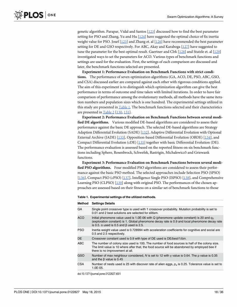
Experiment 1: Performance Evaluation on Benchmark Functions with strict condi-tions. The performance of seven optimization algorithms (GA, ACO, DE, PSO, ABC, GSO,and CSA) discussed earlier are compared against each other with rigorous conditions applied.The aim of this experiment is to distinguish which optimization algorithm can give the bestperformance in terms of outcome and time taken with limited iterations. In order to have faircomparison of performance among the evolutionary methods, all methods have the same itera-tion numbers and population sizes which is one hundred. The experimental settings utilized inthis study are presented in Table 1. The benchmark functions selected and their characteristicsare presented in Table 2 [130, 131].

Experiment 2: Performance Evaluation on Benchmark Functions between several modi-fied DE algorithms. Various modified DE-based algorithms are considered to assess theirperformance against the basic DE approach. The selected DE-based algorithms are StrategyAdaption Differential Evolution (SADE) [132], Adaptive Differential Evolution with OptionalExternal Archive (JADE) [133], Opposition-based Differential Evolution (OBDE) [134], andCompact Differential Evolution (cDE) [135] together with basic Differential Evolution (DE).The performance evaluation is assessed based on the reported fitness on six benchmark func-tions including Sphere, Rosenbrock, Schwefek, Rastrigin, Michalewicz5 and Griewankfunctions.

Experiment 3: Performance Evaluation on Benchmark Functions between several modi-fied PSO algorithms. Four modified PSO algorithms are considered to assess their perfor-mance against the basic PSO method. The selected approaches include Selection PSO (SPSO)[136], Compact PSO (cPSO) [137], Intelligence Single PSO (ISPSO) [138], and ComprehensiveLearning PSO (CLPSO) [139] along with original PSO. The performances of the chosen ap-proaches are assessed based on their fitness on a similar set of benchmark functions to those

Table 1. Experimental settings of the utilized methods.

Method Settings Details

GA Single point crossover type is used with 1 crossover probability. Mutation probability is set to0.01 and 2 best solutions are selected for elitism.

ACO Initial pheromone value used is 1.0E-06 with Q (pheromone update constant) is 20 and q0(exploration constant) is 1. Global pheromone decay rate is 0.9 and local pheromone decay rateis 0.5. α used is 0.5 and β used is 2.5.

PSO Inertia weight value used is 0.728994 with acceleration coefficients for cognitive and social are0.5 and 2.5 respectively.

DE Crossover constant used is 0.9 with type of DE used is DE/best/1/bin.

ABC The number of colony size used is 100. The number of food sources is half of the colony size.The limit value is 10 where after that, the food source will be abandoned by employed bee ifthere is no improvement at all.

GSO Number of max neighbour considered, N is set to 12 with γ value is 0.64. The ρ value is 0.35and the β value is 0.45

CSA Number of nests used is 25 with discover rate of alien eggs, pa is 0.25. Tolerance value is set to1.0E-05.

doi:10.1371/journal.pone.0122827.t001



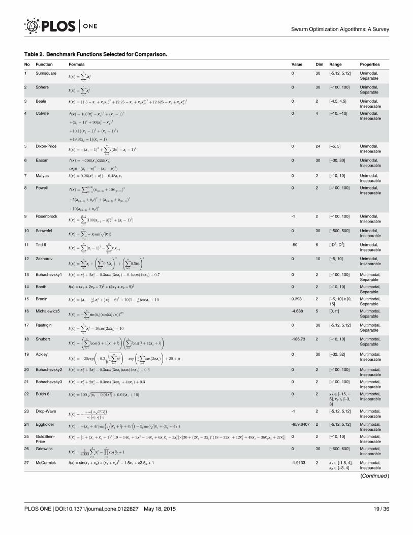
Table 2. Benchmark Functions Selected for Comparison.

No Function Formula Value Dim Range Properties

1 SumsquarefðxÞ ¼

Xni¼1

ix2i

0 30 [-5.12, 5.12] Unimodal,Separable

2 SpherefðxÞ ¼

Xni¼1

x2i

0 30 [–100, 100] Unimodal,Separable

3 Beale fðxÞ ¼ ð1:5� x1 þ x1x2Þ2 þ ð2:25� x1 þ x1x22Þ2 þ ð2:625� x1 þ x1x

32Þ2 0 2 [-4.5, 4.5] Unimodal,

Inseparable

4 Colville fðxÞ ¼ 100ðx21 � x2Þ2 þ ðx1 � 1Þ2

þðx3 � 1Þ2 þ 90ðx23 � x4Þ2

þ10:1ððx2 � 1Þ2 þ ðx4 � 1Þ2Þþ19:8ðx2 � 1Þðx4 � 1Þ

0 4 [–10, –10] Unimodal,Inseparable

5 Dixon-PricefðxÞ ¼ �ðx1 � 1Þ2 þ

Xni¼0

ið2x2i � xi � 1Þ2 0 24 [–5, 5] Unimodal,

Inseparable

6 Easom fðxÞ ¼ �cosðx1Þcosðx2Þexpð�ðx1 � pÞ2 � ðx2 � pÞ2Þ

0 30 [–30, 30] Unimodal,Inseparable

7 Matyas fðxÞ ¼ 0:26ðx21 þ x2

2Þ � 0:48x1x2 0 2 [–10, 10] Unimodal,Inseparable

8 Powell fðxÞ ¼Xðn=kÞ

ði¼1Þ ðxð4i�3Þ þ 10xð4i�2ÞÞ2

þ5ðxð4i�1Þ þ x4 iÞ2 þ ðxð4i�2Þ þ xð4i�1ÞÞ4

þ10ðxð4i�3Þ þ x4 iÞ4

0 2 [–100, 100] Unimodal,Inseparable

9 RosenbrockfðxÞ ¼

Xn�1

i¼1

½100ðxiþ1 � x2i Þ2 þ ðxi � 1Þ2 �

-1 2 [–100, 100] Unimodal,Inseparable

10 SchwefelfðxÞ ¼

Xni¼1

� xisinðffiffiffiffiffiffijxi j

p Þ 0 30 [–500, 500] Unimodal,Inseparable

11 Trid 6fðxÞ ¼

Xni¼1

ðxi � 1Þ2 �Xni¼1

xixi�1

-50 6 [-D2, D2] Unimodal,Inseparable

12 ZakharovfðxÞ ¼

Xni¼1

xi þ Xn

i¼1

0:5ixi

!2

þ Xn

i¼1

0:5ixi

!4 0 10 [–5, 10] Unimodal,Inseparable

13 Bohachevsky1 fðxÞ ¼ x21 þ 2x2

2 � 0:3cosð3px1Þ � 0:4cosð4px2Þ þ 0:7 0 2 [–100, 100] Multimodal,Separable

14 Booth f(x) = (x1 + 2x2 − 7)2 + (2x1 + x2 − 5)2 0 2 [–10, 10] Multimodal,Separable

15 Branin fðxÞ ¼ ðx2 � 5:14p2 x

21 þ 5

p x21 � 6Þ2 þ 10ð1� 1

8pÞcosx1 þ 10 0.398 2 [–5, 10] x [0,15]

Multimodal,Separable

16 Michalewicz5fðxÞ ¼ �

Xni¼1

sinðxiÞðsinðix2i =pÞÞ2m

-4.688 5 [0, π] Multimodal,Separable

17 RastriginfðxÞ ¼

Xni¼1

x2i � 10cosð2pxiÞ þ 10

0 30 [-5.12, 5.12] Multimodal,Separable

18 ShubertfðxÞ ¼

X5i¼1

icosðði þ 1Þx1 þ iÞ! X5

i¼1

icosðði þ 1Þx2 þ iÞ!

-186.73 2 [–10, 10] Multimodal,Separable

19 AckleyfðxÞ ¼ �20exp �0:2

ffiffiffiffiffiffiffiffiffiffiffiffiffiffi1n

Xni¼1

x2i

s !� exp 1

n

Xni¼1

cosð2pxiÞ !

þ 20þ e0 30 [–32, 32] Multimodal,

Inseparable


2 � 0:3cosð3px1Þcosð4px2Þ þ 0:3 0 2 [–100, 100] Multimodal,Inseparable


2 � 0:3cosð3px1 þ 4px2Þ þ 0:3 0 2 [–100, 100] Multimodal,Inseparable

22 Bukin 6 fðxÞ ¼ 100ffiffiffiffiffiffiffiffiffiffiffiffiffiffiffiffiffiffiffiffiffiffiffiffiffiffijx2 � 0:01x2

1 jp þ 0:01jx1 þ 10j 0 2 x1 2 [–15, –

5], x2 2 [–3,3]

Multimodal,Inseparable

23 Drop-WavefðxÞ ¼ � 1þcos

�12ffiffiffiffiffiffiffiffiffix21þx2

2

p �0:5

�x21þx2

2

�þ2

-1 2 [-5.12, 5.12] Multimodal,Inseparable

24 Eggholder fðxÞ ¼ �ðx2 þ 47Þsinffiffiffiffiffiffiffiffiffiffiffiffiffiffiffiffiffiffiffiffiffiffiffiffiffiffiffijx2 þ x1

2þ 47j

q� �� x1sinð

ffiffiffiffiffiffiffiffiffiffiffiffiffiffiffiffiffiffiffiffiffiffiffiffiffiffiffiffiffiffijx1 þ ðx2 þ 47jp Þ -959.6407 2 [-5.12, 5.12] Multimodal,Inseparable

25 GoldStein-Price

fðxÞ ¼ ½1þ ðx1 þ x2 þ 1Þ2ð19� 14x1 þ 3x21 � 14x2 þ 6x1x2 þ 3x2

2 �½30þ ð2x1 � 3x2Þ2ð18� 32x1 þ 12x21 þ 48x2 � 36x1x2 þ 27x22 � 0 2 [–10, 10] Multimodal,

Inseparable

26 GriewankfðxÞ ¼ 1

4000

Xni¼1

x2i �

Yni¼1

cos xiffii

p þ 10 30 [–600, 600] Multimodal,

Inseparable

27 McCormick f(x) = sin(x1 + x2) + (x1 + x2)2− 1.5x1 + x2.52 + 1 -1.9133 2 x1 2 [-1.5, 4],

x2 2 [–3, 4]Multimodal,Inseparable

(Continued)



that have been used in experiment 2 (Sphere, Rosenbrock, Schwefek, Rastrigin, Michalewicz5and Griewank functions).

Benchmark FunctionsEvery benchmark function has its own properties whether it is unimodal, multimodal, separa-ble or non-separable. It is noteworthy that the combination of these properties determines thecomplexity of the functions. A function is considered multimodal if it has two or more local op-tima and it is considered separable if it can be rewritten as a sum of function just from one vari-able. The concept of epistasis or interrelation between variables of the function is related toseparable properties. The concept of epistasis is a concept of genetics where the outcome of onegenetic factor can be governed by the existence of one or more modified genetic factor. Theproblem becomes more complicated if the function is multimodal as well. The global optimumis the value that needs to be estimated during the search process, therefore, the regions aroundlocal minima must be avoided as far as possible. If the local optima are distributed randomly inthe search area, it is considered as the most difficult problem. The aim of optimization processis to obtain the global optima, therefore the regions around local optima should be avoided be-cause the swarm might get stuck in local optima and consider that local optima as the globaloptima. Another important property that determines the difficulty of the problem is the di-mension of the search area. Table 2 presents the list of benchmark functions utilized to assessthe performance of the considered evolutionary methods. The table consists of the name of thebenchmark function, the range, the dimension, the characteristic of the function and its formu-la. The characteristic of the function determines the complexity of the function.

Comparisons and DiscussionThe reported results in this section do not necessarily reflect the performance of the utilizedmethods under all circumstances. The overall performance of such methods can be influencedby the utilized parameterizations and other experimental conditions. However, benchmarkfunctions can be the indicators of how well the optimization algorithms perform under severaldegrees of complexities. In this section, the results of all selected algorithms tested on thirtybenchmark functions are presented and discussed.

Performance Evaluation on Benchmark FunctionsIn this experiment, the performance of optimization techniques selected are assessed on a vari-ety of benchmark functions using MATLAB2011 on a CORE i5 CPU with 2GB RAM and havebeen run thirty times. The average result of the runs (Mean), standard deviation (SD) and timetaken (in seconds) to complete each run are reported in Tables 3, 4 and 5. If the mean value isless than 1.000E-10, then the result is reported as 0.000E+00. In this experiment, only basic ver-sions of SI techniques are considered and no modifications are applied. Algorithm codes are

Table 2. (Continued)

No Function Formula Value Dim Range Properties

28 PermfðxÞ ¼

Xnk¼1

Xni¼1

ðik þ bÞðxi=iÞk � 1Þ2 0 4 [-D, D] Multimodal,Inseparable

29 Schaffer 2 fðxÞ ¼ 0:5þ sin2 ðffiffiffiffiffiffiffiffiffix21þx2

2

pÞ�0:5�

1þ0:0001

� ffiffiffiffiffiffiffiffiffix21þx2

2

p ��2 0 2 [–100, 100] Multimodal,Inseparable

30 Schaffer 4 fðxÞ ¼ 0:5þ cosðsinðjx21þx2

2ÞÞ�0:5

ð1þ0:0001ðx21þx2

2ÞÞ2

0 2 [–100, 100] Multimodal,Inseparable




adapted from several sources and are modified to be compatible with our experimental setup[158–161].

Tables 3 and 4. The first two benchmark functions in Table 3 and Table 4 (e.g., Sphereand Sumsquare) are unimodal and separable with a theoretical minimization value of zero. InSphere, the result which is closest to the theoretical optimal value is acquired by DE with5.5942E+03 and GA becomes the second best with 6.4415E+03. In the Sumsquare function,none of the algorithms achieved the best minimization performance but PSO has become thebest algorithm with 3.7357E+00 and ACO has become the second best with 5.6363E+00. Thethird best is DE where it managed to achieve 7.7637E+00. The next ten functions in these tables

Table 3. Benchmark Functions Comparison of mean error (Mean ± SD) and time (Seconds) on Several Optimization Techniques.

Function GA ACO PSO DE

Sphere (Separable) 6.4415E+03 1.7596E+04 1.0454E+05 5.5942E+03

±1.6876E+03 ±1.8603E+03 ±7.1998E+04 ±1.5091E+03

(4.3531s) (7.3219s) (2.8906s) (10.9984s)

Sumsquare (Separable) 1.7376E+01 5.6363E+00 3.7357E+00 7.7637E+00

±3.7449E-15 ±4.0719E-01 ±1.8203E-01 ±1.4868E+00

(3.8938s) (6.9031s) (3.1422s) (11.4047s)

Beale (Inseparable) 7.0313E-01 7.0313E-01 0.0000E+00 0.0000E+00

±0.0000E+00 ±0.0000E+00 ±0.0000E+00 ±0.0000E+00

(3.1078s) (2.8938s) (1.9094s) (4.9531s)

Colville (Inseparable) 0.0000E+00 6.6160E+01 0.0000E+00 1.4017E+00

±0.0000E+00 ±3.7940E+01 ±0.0000E+00 ±2.1101E+00

(2.6875s) (2.2703s) (1.8922s) (4.7859s)

Dixon-Price (Inseparable) 1.1029E+05 1.8708E+06 4.9633E+06 1.3145E+04

±3.4184E+04 ±4.3444E+05 ±3.4317E+06 ±6.3822E+03

(4.1063s) (6.7469s) (3.1000s) (11.3109s)

Easom (Inseparable) -1.0000E+00 -1.0000E+00 -1.0000E+00 -1.0000E+00

±0.0000E+00 ±0.0000E+00 ±0.0000E+00 ±0.0000E+00

(6.0281s) (2.0016s) (1.8875s) (4.8734s)

Matyas (Inseparable) 0.0000E+00 0.0000E+00 0.0000E+00 0.0000E+00

±0.0000E+00 ±0.0000E+00 ±0.0000E+00 ±0.0000E+00

(2.7453s) (2.0500s) (2.0250s) (5.0875s)

Powell (Inseparable) 4.2230E+02 9.4665E+03 1.0689E+04 3.1662E+02

±1.2382E+02 ±1.4600E+03 ±3.7167E+03 ±1.3003E+02

(3.9266s) (5.5594s) (2.6859s) (9.4516s)

Rosenbrock (Inseparable) 1.2493E+07 1.1051E+08 7.0289E+08 3.8901E+06

±8.6725E+06 ±2.1694E+07 ±4.8937E+08 ±2.2417E+06

(4.0797s) (6.9359s) (2.9797s) (11.0344s)

Schwefel (Inseparable) 5.2808E+03 3.2250E+03 7.0202E+03 5.6371E+03

±6.2830E+02 ±4.5211E+02 ±1.2171E+02 ±5.9306E+02

(4.4391s) (9.9703s) (2.8094s) (12.5828s)

Trid6 (Inseparable) -2.5000E+01 -2.4300E+01 -5.0000E+01 -4.7697E+01

±1.2293E+01 ±9.3339E+00 ±0.0000E+00 ±5.0327E+00

(3.1516s) (2.7422s) (2.0859s) (5.8891s)

Zakharov (Inseparable) 2.9550E+01 7.1088E+01 0.0000E+00 0.0000E+00

±2.0370E+01 ±1.4866E+01 ±0.0000E+00 ±0.0000E+00

(3.8078s) (3.4719s) (2.3953s) (6.8844s)




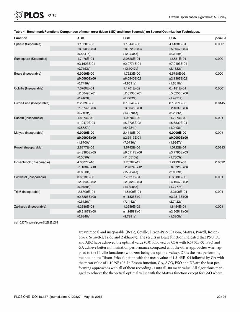
are unimodal and inseparable (Beale, Coville, Dixon-Price, Easom, Matyas, Powell, Rosen-brock, Schwefel, Trid6 and Zakharov). The results in Beale function indicated that PSO, DEand ABC have achieved the optimal value (0.0) followed by CSA with 6.5750E-02. PSO andGA achieve better minimization performance compared with the other approaches when ap-plied to the Coville functions (with zero being the optimal value). DE is the best performingmethod on the Dixon-Price function with the mean value of 1.3145E+04 followed by GA withthe mean value of 1.1029E+05. In Easom function, GA, ACO, PSO and DE are the best per-forming approaches with all of them recording -1.0000E+00 mean value. All algorithms man-aged to achieve the theoretical optimal value with the Matyas function except for GSO where


Function ABC GSO CSA p-value

Sphere (Separable) 1.1820E+05 1.1844E+06 4.4138E+04 0.0001

±8.3508E+03 ±8.0723E+04 ±5.5047E+04

(0.5641s) (12.3234s) (2.0959s)

Sumsquare (Separable) 1.7476E+01 2.0526E+01 1.6531E+01 0.0001

±3.1623E-01 ±2.9771E-01 ±7.9493E-01

(0.7153s) (12.1047s) (2.1822s)

Beale (Inseparable) 0.0000E+00 1.7223E+00 6.5750E-02 0.0001

±0.0000E+00 ±6.0540E-02 ±2.1365E-02

(0.7496s) (4.9531s) (1.5618s)

Colville (Inseparable) 7.3760E+01 1.1701E+02 6.4181E+01 0.0001

±2.8049E+01 ±2.6130E+01 ±5.5250E+00

(0.4483s) (6.7732s) (1.4921s)

Dixon-Price (Inseparable) 2.2939E+06 3.1354E+08 8.1887E+05 0.0145

±1.5742E+06 ±3.6645E+08 ±2.4639E+06

(6.7469s) (14.2784s) (2.2086s)

Easom (Inseparable) 1.8974E-03 1.0670E+00 -1.7374E-03 0.001

±1.2470E-04 ±5.3736E-02 ±5.6839E-04

(0.5687s) (6.4734s) (1.2498s)

Matyas (Inseparable) 0.0000E+00 2.4540E+00 0.0000E+00 0.001

±0.0000E+00 ±2.6413E-01 ±0.0000E+00

(1.8700s) (7.0736s) (1.9967s)

Powell (Inseparable) 2.6977E+05 3.6742E+06 1.0722E+04 0.0913

±4.3360E+05 ±6.5117E+06 ±3.7790E+03

(0.5690s) (11.5516s) (1.7003s)

Rosenbrock (Inseparable) 4.8807E+10 1.7626E+12 1.2493E+07 0.0592

±1.1684E+10 ±2.7674E+12 ±8.6725E+06

(0.6313s) (15.2344s) (2.0009s)

Schwefel (Inseparable) 3.6619E+03 7.7821E+04 6.6619E+03 0.001

±2.3244E+02 ±2.0826E+03 ±4.1047E+02

(0.9188s) (14.6285s) (1.7777s)

Trid6 (Inseparable) -2.6800E+01 -1.5100E+01 -3.3100E+01 0.001

±2.8206E+00 ±1.1836E+01 ±3.2813E+00

(0.5126s) (7.1442s) (2.7422s)

Zakharov (Inseparable) 9.2688E+01 1.3259E+02 1.8454E+01 0.001

±5.5187E+00 ±1.1658E+01 ±2.9051E+00

(0.6348s) (8.7891s) (1.3908s)




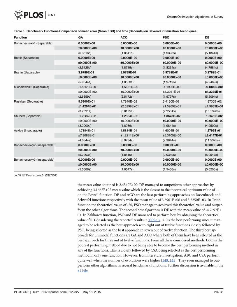
the mean value obtained is 2.4540E+00. DE managed to outperform other approaches byachieving 3.1662E+02 mean value which is the closest to the theoretical optimum value of -1on the Powell function. DE and ACO are the best performing approaches on Rosenbrock andSchwefel functions respectively with the mean value of 3.8901E+06 and 3.2250E+03. In Trid6function the theoretical value of -50, PSO manage to achieved this theoretical value and outper-form the other algorithms. The second best algorithm is DE with the mean value of -4.7697E+01. In Zakharov function, PSO and DE managed to perform best by obtaining the theoreticalvalue of 0. Considering the reported results in Table 3, DE is the best performing since it man-aged to be selected as the best approach with eight out of twelve functions closely followed byPSO, being selected as the best approach in seven out of twelve function. The third best ap-proach for unimodal functions are GA and ACO where both of them have been selected as thebest approach for three out of twelve functions. From all these considered methods, GSO is thepoorest performing method due to not being able to become the best performing method inany of the functions. This is closely followed by CSA being selected as the best performingmethod in only one function. However, from literature investigation, ABC and CSA performquite well when the number of evolutions were higher [140, 141]. They even managed to out-perform other algorithms in several benchmark functions. Further discussion is available in theS1 File.



Bohachecvsky1 (Separable) 0.0000E+00 0.0000E+00 0.0000E+00 0.0000E+00

±0.0000E+00 ±0.0000E+00 ±0.0000E+00 ±0.0000E+00

(6.3516s) (1.8641s) (1.9328s) (5.1844s)

Booth (Separable) 0.0000E+00 0.0000E+00 0.0000E+00 0.0000E+00

±0.0000E+00 ±0.0000E+00 ±0.0000E+00 ±0.0000E+00

(2.5125s) (1.8719s) (1.8234s) (4.7984s)

Branin (Separable) 3.9789E-01 3.9789E-01 3.9789E-01 3.9789E-01

±0.0000E+00 ±0.0000E+00 ±0.0000E+00 ±0.0000E+00

(5.9844s) (1.8563s) (1.9719s) (4.9469s)

Michalewciz5 (Separable) -1.5651E+00 -1.5651E+00 -1.1906E+00 -4.1803E+00

±0.0000E+00 ±0.0000E+00 ±3.3261E-01 ±4.2335E-01

(2.6859s) (2.5172s) (1.9797s) (5.3094s)

Rastrigin (Separable) 5.5900E+01 1.7840E+02 5.4130E+02 1.8730E+02

±1.4294E+01 ±2.5299E+01 ±1.5969E+01 ±1.9989E+01

(3.7891s) (6.8125s) (2.9531s) (10.1328s)

Shubert (Separable) -1.2884E+02 -1.2884E+02 -1.8673E+02 -1.8673E+02

±0.0000E+00 ±0.0000E+00 ±0.0000E+00 ±0.0000E+00

(3.2000s) (1.8266s) (1.9844s) (4.9500s)

Ackley (Inseparable) 1.7194E+01 1.5884E+01 1.6004E+01 1.2795E+01

±7.9083E-01 ±1.2211E+00 ±5.3105E+00 ±8.4147E-01

(4.0344s) (8.9734s) (2.9844s) (11.5375s)

Bohachecvsky2 (Inseparable) 0.0000E+00 0.0000E+00 0.0000E+00 0.0000E+00

±0.0000E+00 ±0.0000E+00 ±0.0000E+00 ±0.0000E+00

(5.7203s) (1.8516s) (2.0359s) (5.0547s)

Bohachecvsky3 (Inseparable) 0.0000E+00 0.0000E+00 0.0000E+00 0.0000E+00

±0.0000E+00 ±0.0000E+00 ±0.0000E+00 ±0.0000E+00

(5.5688s) (1.8547s) (1.9438s) (5.0203s)




Tables 5, 6, 7 and 8. Tables 5 to 8 are focusing on multimodal functions with the first sixfunctions (Bohachecvsky1, Booth, Branin, Michalewicz5, Rastrigin and Shubert) being separa-ble. The best performance for Bohachecvsky1 is shared between five algorithms of GA, ACO,PSO, DE and ABC where they managed to find the theoretical value of 0. The second and thirdfunctions utilized are Booth and Branin functions where in these functions the best perfor-mance is shared between six algorithms (GA, ACO, PSO, DE, ABC and CSA). The forth func-tion is Michalewicz5 with theoretical value of -4.687658. DE achieved the closest average pervalue to the theoretical value with -4.1803. In Rastrigin with 0 theoretical value, GA managedto outperform other algorithms with the mean value of 5.5900E+01. In Shuber function, PSOand DE managed to acquire the theoretical value of -186.7309.

The rest of the functions considered in these tables are multimodal and inseparable. Thefunctions that are this type of characteristic are Ackley, Bohachecvsky2, Bohachecvsky3,Bukin6, Drop-Wave, Egg Holder, Goldstein-Price, Griewank, McCormick, Perm, Schaffer2and Schaffer4. Considering these functions, DE, became the best performing approach achiev-ing the best performance in 11 out of 12 functions. DE has performed best in all functions ex-cept Egg-Holder where GA is the best performing approaches. In Egg-Holder, GA managed torecord a mean value of -9.1540E+02 which is the closest to the optimal value of -959.6407. PSOand GA shared the second best performing approaches where they become the best algorithm



Bohachecvsky1 (Separable) 0.0000E+00 1.7640E+00 8.2066E-03 0.001

±0.0000E+00 ±8.0414E-02 ±8.0204E-03

(0.5953s) (6.9719s) (1.0634s)

Booth (Separable) 0.0000E+00 4.6000E+00 0.0000E+00 0.001

±0.0000E+00 ±2.3002E-01 ±0.0000E+00

(0.5858s) (4.7984s) (1.0859s)

Branin (Separable) 3.9789E-01 3.7481E+01 3.9789E-01 0.001

±0.0000E+00 ±8.6588E-01 ±0.0000E+00

(0.4856s) (6.4852s) (1.0778s)

Michalewciz5 (Separable) -3.5684E+00 -9.9061E-01 -1.5436E+00 0.001

±3.2433E-02 ±2.5724E-01 ±6.7793E-02

(0.5264s) (6.1347s) (1.9797s)

Rastrigin (Separable) 1.2382E+05 1.2679E+08 1.3202E+05 0.001

±1.1630E+04 ±1.3932E+07 ±1.6245E+04

(0.6391s) (12.3106s) (2.0863s)

Shubert (Separable) -1.2942E+01 -8.8424E+00 -2.7642E+01 0.001

±3.1623E-01 ±0.0000E+00 ±2.1499E+00

(0.4758s) (6.5500s) (1.0811s)

Ackley (Inseparable) 2.0681E+01 1.9896E+01 1.2795E+01 0.001

±3.8721E-02 ±5.3227E-01 ±8.4147E-01

(0.9875s) (12.1059s) (0.9875s)

Bohachecvsky2 (Inseparable) 4.7124E-01 3.0422E+01 5.4223E+00 0.001

±2.8573E-01 ±6.9014E+00 ±2.6812E+00

(0.4566s) (6.7005s) (1.1120s)

Bohachecvsky3 (Inseparable) 5.2233E-01 1.2818E+01 2.8223E+00 0.001

±3.3498E-01 ±4.6593E-01 ± 4.6749E-01

(0.4595s) (6.1463s) (1.0485s)




in eight out of twelve function. It is noticeable that GA, ACO, PSO and DE share the best per-forming approaches in Bohachecvsky2, Bohachecvsky3, Bukin6, Drop-Wave, Goldstein-Price,McCormick and Schaffer functions where all of them managed to find the theoretical optimalvalue of zero. Within the Griewank and Perm functions, DE has become the best performingapproach with a mean value of 1.1282E+00 and 0 respectively. PSO and DE once again havebecome the best methods when applied to Schaffer2 function where they managed to obtain anoptimal value of 0.

Overall performance. The results presented in Tables 3 to 8 can also be investigated basedon the characteristics of the fitness functions utilized in the study. Considering categories of i)Unimodal and Separable (US), ii) Unimodal and Inseparable (UI), iii) Multimodal and Separa-ble (MS), iv) Multimodal and Inseparable (MI), v) Multimodal (M), vi) Unimodal (U), vii) Sep-arable (S), and viii) Inseparable (I), Table 9 is formed. Considering the results presented inTable 9, DE seems to be the best overall performing approach, outperforming other methodsin 24 out of 30 functions followed by PSO with the best performance in 19 out of 30. The thirdbest is GA with 14 out 30 best performance and closely followed by ACO with 13 out of 30 bestperformance. ABC, and CSA reached the best performance in 6 and 3 out of 30 functions re-spectively. Focusing on the breakdown results it is noticeable that DE has been the best per-forming method in all categories. However, in terms of time consumed to complete the



Bukin 6 (Inseparable) 0.0000E+00 0.0000E+00 0.0000E+00 0.0000E+00

±0.0000E+00 ±0.0000E+00 ±0.0000E+00 ±0.0000E+00

(2.4766s) (1.8250s) (1.9625s) (4.9813s)

Drop-Wave (Inseparable) -1.0000E+00 -1.0000E+00 -1.0000E+00 -1.0000E+00

±0.0000E+00 ±0.0000E+00 ±0.0000E+00 ±0.0000E+00

(2.7391s) (2.3813s) (1.9641s) (5.3031s)

Egg Holder (Insepearable) -9.1540E+02 -8.4202E+02 -8.9632E+02 -9.0219E+02

±3.0628E+01 ±5.5959E+01 ±5.7481E+01 ±6.0614E+01

(2.8531s) (2.6031s) (1.9313s) (5.2063s)

Goldstein-Price (Inseparable) 3.0000E+00 3.0000E+00 3.0000E+00 3.0000E+00

±0.0000E+00 ±0.0000E+00 ±0.0000E+00 ±0.0000E+00

(2.4531s) (2.6172s) (1.8375s) (5.0313s)

Griewank (Inseparable) 1.2194E+00 1.1711E+00 3.2000E+00 1.1282E+00

±8.9937E-02 ±2.9271E-02 ±1.5451E+00 ±4.0468E-02

(4.0516s) (10.9766s) (3.0766s) (11.8531s)

McCormick (Inseparable) -1.9134E+00 -1.9134E+00 -1.9133E+00 -1.9132E+00

±0.0000E+00 ±0.0000E+00 ±0.0000E+00 ±0.0000E+00

(2.7969s) (2.3266s) (1.8844s) (5.0672s)

Perm (Inseparable) 7.2815E+02 7.2815E+02 2.9684E+04 0.0000E+00

±0.0000E+00 ±0.0000E+00 ±1.8921E+04 ±0.0000E+00

(3.0047s) (2.5734s) (2.1234s) (5.2578s)

Schaffer 2 (Inseparable) 3.9880E-04 1.4299E-02 0.0000E+00 0.0000E+00

±8.4075E-04 ±1.9474E-02 ±0.0000E+00 ±0.0000E+00

(2.4000s) (2.2672s) (2.0328s) (5.3063s)

Schaffer 4 (Inseparable) 0.0000E+00 0.0000E+00 0.0000E+00 0.0000E+00

±0.0000E+00 ±0.0000E+00 ±0.0000E+00 ±0.0000E+00

(2.7844s) (2.4375s) (1.9438s) (5.3531s)




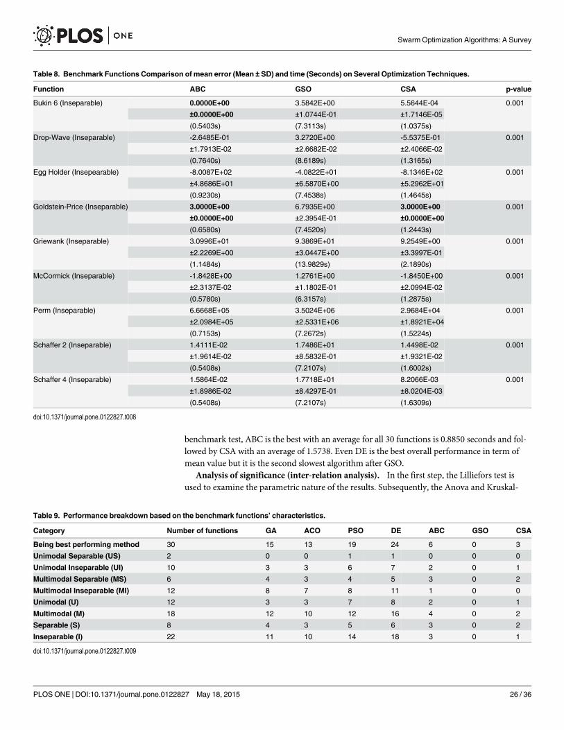
benchmark test, ABC is the best with an average for all 30 functions is 0.8850 seconds and fol-lowed by CSA with an average of 1.5738. Even DE is the best overall performance in term ofmean value but it is the second slowest algorithm after GSO.

Analysis of significance (inter-relation analysis). In the first step, the Lilliefors test isused to examine the parametric nature of the results. Subsequently, the Anova and Kruskal-



Bukin 6 (Inseparable) 0.0000E+00 3.5842E+00 5.5644E-04 0.001

±0.0000E+00 ±1.0744E-01 ±1.7146E-05

(0.5403s) (7.3113s) (1.0375s)

Drop-Wave (Inseparable) -2.6485E-01 3.2720E+00 -5.5375E-01 0.001

±1.7913E-02 ±2.6682E-02 ±2.4066E-02

(0.7640s) (8.6189s) (1.3165s)

Egg Holder (Insepearable) -8.0087E+02 -4.0822E+01 -8.1346E+02 0.001

±4.8686E+01 ±6.5870E+00 ±5.2962E+01

(0.9230s) (7.4538s) (1.4645s)

Goldstein-Price (Inseparable) 3.0000E+00 6.7935E+00 3.0000E+00 0.001

±0.0000E+00 ±2.3954E-01 ±0.0000E+00

(0.6580s) (7.4520s) (1.2443s)

Griewank (Inseparable) 3.0996E+01 9.3869E+01 9.2549E+00 0.001

±2.2269E+00 ±3.0447E+00 ±3.3997E-01

(1.1484s) (13.9829s) (2.1890s)

McCormick (Inseparable) -1.8428E+00 1.2761E+00 -1.8450E+00 0.001

±2.3137E-02 ±1.1802E-01 ±2.0994E-02

(0.5780s) (6.3157s) (1.2875s)

Perm (Inseparable) 6.6668E+05 3.5024E+06 2.9684E+04 0.001

±2.0984E+05 ±2.5331E+06 ±1.8921E+04

(0.7153s) (7.2672s) (1.5224s)

Schaffer 2 (Inseparable) 1.4111E-02 1.7486E+01 1.4498E-02 0.001

±1.9614E-02 ±8.5832E-01 ±1.9321E-02

(0.5408s) (7.2107s) (1.6002s)

Schaffer 4 (Inseparable) 1.5864E-02 1.7718E+01 8.2066E-03 0.001

±1.8986E-02 ±8.4297E-01 ±8.0204E-03

(0.5408s) (7.2107s) (1.6309s)


Table 9. Performance breakdown based on the benchmark functions’ characteristics.

Category Number of functions GA ACO PSO DE ABC GSO CSA

Being best performing method 30 15 13 19 24 6 0 3

Unimodal Separable (US) 2 0 0 1 1 0 0 0

Unimodal Inseparable (UI) 10 3 3 6 7 2 0 1

Multimodal Separable (MS) 6 4 3 4 5 3 0 2

Multimodal Inseparable (MI) 12 8 7 8 11 1 0 0

Unimodal (U) 12 3 3 7 8 2 0 1

Multimodal (M) 18 12 10 12 16 4 0 2

Separable (S) 8 4 3 5 6 3 0 2

Inseparable (I) 22 11 10 14 18 3 0 1




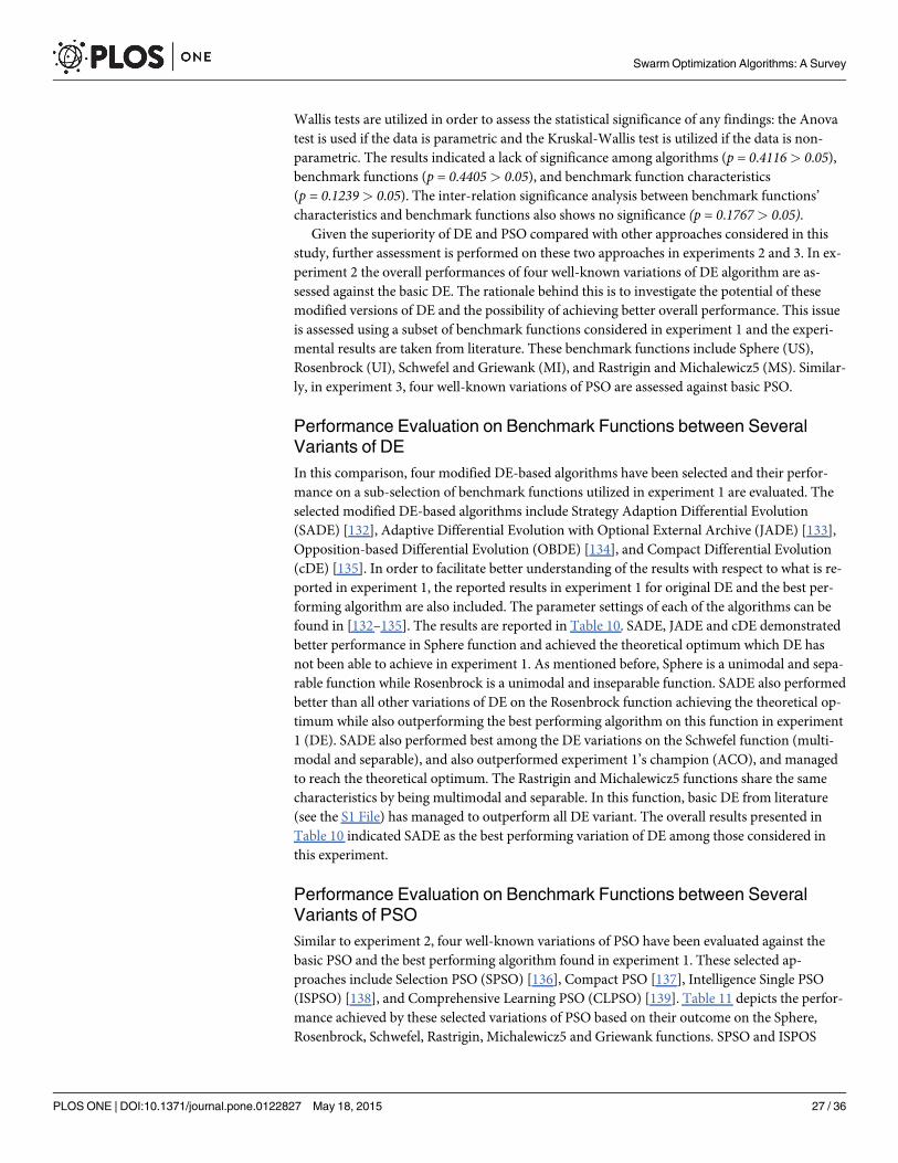
Wallis tests are utilized in order to assess the statistical significance of any findings: the Anovatest is used if the data is parametric and the Kruskal-Wallis test is utilized if the data is non-parametric. The results indicated a lack of significance among algorithms (p = 0.4116> 0.05),benchmark functions (p = 0.4405> 0.05), and benchmark function characteristics(p = 0.1239> 0.05). The inter-relation significance analysis between benchmark functions’characteristics and benchmark functions also shows no significance (p = 0.1767> 0.05).

Given the superiority of DE and PSO compared with other approaches considered in thisstudy, further assessment is performed on these two approaches in experiments 2 and 3. In ex-periment 2 the overall performances of four well-known variations of DE algorithm are as-sessed against the basic DE. The rationale behind this is to investigate the potential of thesemodified versions of DE and the possibility of achieving better overall performance. This issueis assessed using a subset of benchmark functions considered in experiment 1 and the experi-mental results are taken from literature. These benchmark functions include Sphere (US),Rosenbrock (UI), Schwefel and Griewank (MI), and Rastrigin and Michalewicz5 (MS). Similar-ly, in experiment 3, four well-known variations of PSO are assessed against basic PSO.

Performance Evaluation on Benchmark Functions between SeveralVariants of DEIn this comparison, four modified DE-based algorithms have been selected and their perfor-mance on a sub-selection of benchmark functions utilized in experiment 1 are evaluated. Theselected modified DE-based algorithms include Strategy Adaption Differential Evolution(SADE) [132], Adaptive Differential Evolution with Optional External Archive (JADE) [133],Opposition-based Differential Evolution (OBDE) [134], and Compact Differential Evolution(cDE) [135]. In order to facilitate better understanding of the results with respect to what is re-ported in experiment 1, the reported results in experiment 1 for original DE and the best per-forming algorithm are also included. The parameter settings of each of the algorithms can befound in [132–135]. The results are reported in Table 10. SADE, JADE and cDE demonstratedbetter performance in Sphere function and achieved the theoretical optimum which DE hasnot been able to achieve in experiment 1. As mentioned before, Sphere is a unimodal and sepa-rable function while Rosenbrock is a unimodal and inseparable function. SADE also performedbetter than all other variations of DE on the Rosenbrock function achieving the theoretical op-timum while also outperforming the best performing algorithm on this function in experiment1 (DE). SADE also performed best among the DE variations on the Schwefel function (multi-modal and separable), and also outperformed experiment 1’s champion (ACO), and managedto reach the theoretical optimum. The Rastrigin and Michalewicz5 functions share the samecharacteristics by being multimodal and separable. In this function, basic DE from literature(see the S1 File) has managed to outperform all DE variant. The overall results presented inTable 10 indicated SADE as the best performing variation of DE among those considered inthis experiment.

Performance Evaluation on Benchmark Functions between SeveralVariants of PSOSimilar to experiment 2, four well-known variations of PSO have been evaluated against thebasic PSO and the best performing algorithm found in experiment 1. These selected ap-proaches include Selection PSO (SPSO) [136], Compact PSO [137], Intelligence Single PSO(ISPSO) [138], and Comprehensive Learning PSO (CLPSO) [139]. Table 11 depicts the perfor-mance achieved by these selected variations of PSO based on their outcome on the Sphere,Rosenbrock, Schwefel, Rastrigin, Michalewicz5 and Griewank functions. SPSO and ISPOS



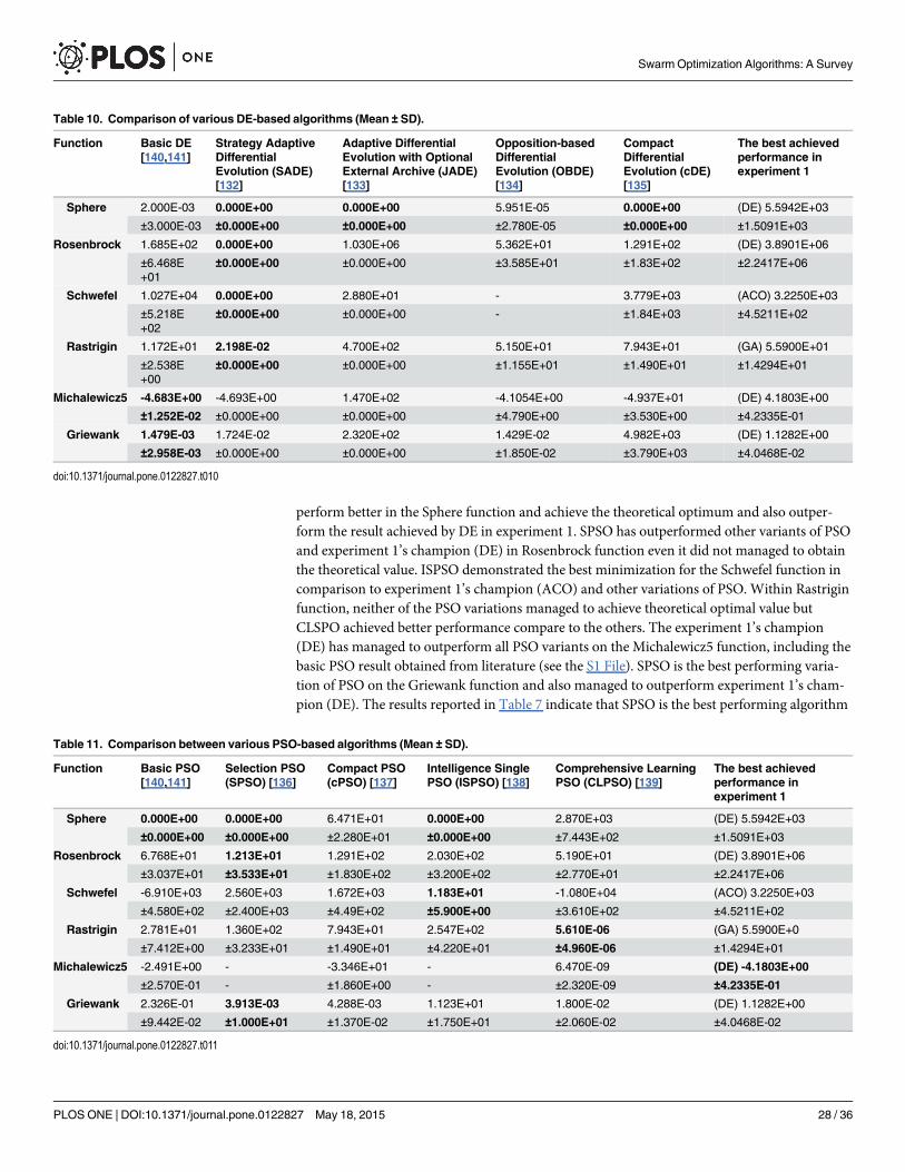
perform better in the Sphere function and achieve the theoretical optimum and also outper-form the result achieved by DE in experiment 1. SPSO has outperformed other variants of PSOand experiment 1’s champion (DE) in Rosenbrock function even it did not managed to obtainthe theoretical value. ISPSO demonstrated the best minimization for the Schwefel function incomparison to experiment 1’s champion (ACO) and other variations of PSO. Within Rastriginfunction, neither of the PSO variations managed to achieve theoretical optimal value butCLSPO achieved better performance compare to the others. The experiment 1’s champion(DE) has managed to outperform all PSO variants on the Michalewicz5 function, including thebasic PSO result obtained from literature (see the S1 File). SPSO is the best performing varia-tion of PSO on the Griewank function and also managed to outperform experiment 1’s cham-pion (DE). The results reported in Table 7 indicate that SPSO is the best performing algorithm

Table 10. Comparison of various DE-based algorithms (Mean ± SD).

Function Basic DE[140,141]

Strategy AdaptiveDifferentialEvolution (SADE)[132]

Adaptive DifferentialEvolution with OptionalExternal Archive (JADE)[133]

Opposition-basedDifferentialEvolution (OBDE)[134]

CompactDifferentialEvolution (cDE)[135]

The best achievedperformance inexperiment 1

Sphere 2.000E-03 0.000E+00 0.000E+00 5.951E-05 0.000E+00 (DE) 5.5942E+03

±3.000E-03 ±0.000E+00 ±0.000E+00 ±2.780E-05 ±0.000E+00 ±1.5091E+03

Rosenbrock 1.685E+02 0.000E+00 1.030E+06 5.362E+01 1.291E+02 (DE) 3.8901E+06

±6.468E+01

±0.000E+00 ±0.000E+00 ±3.585E+01 ±1.83E+02 ±2.2417E+06

Schwefel 1.027E+04 0.000E+00 2.880E+01 - 3.779E+03 (ACO) 3.2250E+03

±5.218E+02

±0.000E+00 ±0.000E+00 - ±1.84E+03 ±4.5211E+02

Rastrigin 1.172E+01 2.198E-02 4.700E+02 5.150E+01 7.943E+01 (GA) 5.5900E+01

±2.538E+00

±0.000E+00 ±0.000E+00 ±1.155E+01 ±1.490E+01 ±1.4294E+01

Michalewicz5 -4.683E+00 -4.693E+00 1.470E+02 -4.1054E+00 -4.937E+01 (DE) 4.1803E+00

±1.252E-02 ±0.000E+00 ±0.000E+00 ±4.790E+00 ±3.530E+00 ±4.2335E-01

Griewank 1.479E-03 1.724E-02 2.320E+02 1.429E-02 4.982E+03 (DE) 1.1282E+00

±2.958E-03 ±0.000E+00 ±0.000E+00 ±1.850E-02 ±3.790E+03 ±4.0468E-02


Table 11. Comparison between various PSO-based algorithms (Mean ± SD).

Function Basic PSO[140,141]

Selection PSO(SPSO) [136]

Compact PSO(cPSO) [137]

Intelligence SinglePSO (ISPSO) [138]

Comprehensive LearningPSO (CLPSO) [139]

The best achievedperformance inexperiment 1

Sphere 0.000E+00 0.000E+00 6.471E+01 0.000E+00 2.870E+03 (DE) 5.5942E+03

±0.000E+00 ±0.000E+00 ±2.280E+01 ±0.000E+00 ±7.443E+02 ±1.5091E+03

Rosenbrock 6.768E+01 1.213E+01 1.291E+02 2.030E+02 5.190E+01 (DE) 3.8901E+06

±3.037E+01 ±3.533E+01 ±1.830E+02 ±3.200E+02 ±2.770E+01 ±2.2417E+06

Schwefel -6.910E+03 2.560E+03 1.672E+03 1.183E+01 -1.080E+04 (ACO) 3.2250E+03

±4.580E+02 ±2.400E+03 ±4.49E+02 ±5.900E+00 ±3.610E+02 ±4.5211E+02

Rastrigin 2.781E+01 1.360E+02 7.943E+01 2.547E+02 5.610E-06 (GA) 5.5900E+0

±7.412E+00 ±3.233E+01 ±1.490E+01 ±4.220E+01 ±4.960E-06 ±1.4294E+01

Michalewicz5 -2.491E+00 - -3.346E+01 - 6.470E-09 (DE) -4.1803E+00

±2.570E-01 - ±1.860E+00 - ±2.320E-09 ±4.2335E-01

Griewank 2.326E-01 3.913E-03 4.288E-03 1.123E+01 1.800E-02 (DE) 1.1282E+00

±9.442E-02 ±1.000E+01 ±1.370E-02 ±1.750E+01 ±2.060E-02 ±4.0468E-02




among the considered variations of PSO since it is selected as the best PSO variation in 3 out of6 benchmark functions in addition to being able to outperform the best performing approachin experiment 1 in 3 of the benchmark functions (Sphere, Rosenbrock and Griewank). ISPSOis the second best performing variation of PSO by outperforming other variations in 2 bench-mark functions and also outperformed experiment 1’s champion (Sphere and Schwefel).CLPSO is the third best performance where it managed to outperform other competitors inRastrigin function. cPSO is the least favourable variation among the selected methods becauseof incompetency to outperform others in any function listed.

ConclusionsThis study was concerned with overall performance of various Swarm Intelligence (SI) basedapproaches and aimed to provide a comparison among the well-known SI-based approaches.A set of methods including Genetic algorithm (GA), Ant Colony Optimization (ACO), ParticleSwarm Optimization (PSO), Differential Evolution (DE), Artificial Bee Colony (ABC), Glow-worm Swarm Optimization (GSO), and Cuckoo Search Algorithm (CSA) are considered and aselection of thirty benchmark functions that have been utilized in MATLAB to measure theperformance of these approaches. These benchmark functions cover a range of characteristicsincluding unimodal, multimodal, separable, and inseparable. The results indicated the superi-ority of DE with the ability to outperform or perform equally to the best algorithm in 24 out of30 functions. DE performed very well on multimodal functions, being selected as the best per-forming approach in 11 out of 12 such functions. This performance repeater in unimodal andinseparable functions in which DE outperformed others in 8 out of 12 and 18 out of 22 func-tions respectively. PSO is the second best approach that outperformed or performed equally tothe best algorithm in 18 out of 30 functions and follows by GA with 14 out of 30. Two extra ex-periments are offered to capture the performance of four well-known modified versions ofPSO and DE on a sub set of 6 benchmark functions. These variations included Strategy Adap-tion Differential Evolution (SADE) [132], Adaptive Differential Evolution with Optional Exter-nal Archive (133) [134], Opposition-based Differential Evolution (OBDE) [88], CompactDifferential Evolution (cDE) [135], Selection PSO (SPSO) [136], Compact PSO [137], Intelli-gence Single PSO (ISPSO) [138], and Comprehensive Learning PSO (CLPSO) [139]. The re-sults identified SADE and SPSO as the best performing approaches.

Supporting InformationS1 PRISMA Checklist.(DOCX)

S1 File. Supporting text and tables. Table A. Parameter setting utilized by literature studiesfor each algorithm. Table B. Benchmark Functions Selected for Comparison. Table C. Bench-mark Functions Comparison between Several Optimization Techniques (Mean ± SD).Table D. Continued Benchmark Functions Comparison between Several Optimization Tech-niques (Mean ± SD). Table E. Continued Benchmark Functions Comparison between SeveralOptimization Techniques (Mean ± SD). Table F. Continued Benchmark Functions Compari-son between Several Optimization Techniques (Mean ± SD). Table G. Performance breakdownbased on the benchmark functions’ characteristics. Table H. Benchmark Functions Compari-son with an offset of mean error (Mean ± SD) and time (Seconds) on several OptimizationTechniques. Table I. Benchmark Functions Comparison with an offset of mean error(Mean ± SD) and time (Seconds) on several Optimization Techniques. Table J. BenchmarkFunctions Comparison with an offset of mean error (Mean ± SD) and time (Seconds) on



http://www.plosone.org/article/fetchSingleRepresentation.action?uri=info:doi/10.1371/journal.pone.0122827.s001

http://www.plosone.org/article/fetchSingleRepresentation.action?uri=info:doi/10.1371/journal.pone.0122827.s002

several Optimization Techniques. Table K. Benchmark Functions Comparison with an offsetof mean error (Mean ± SD) and time (Seconds) on several Optimization Techniques. Table L.Benchmark Functions Comparison with an offset of mean error (Mean ± SD) and time (Sec-onds) on several Optimization Techniques. Table M. Benchmark Functions Comparison withan offset of mean error (Mean ± SD) and time (Seconds) on several Optimization Techniques.Table N. Comparison of various DE-based algorithms (Mean ± SD).(DOCX)

Author ContributionsConceived and designed the experiments: MNAWAA. Performed the experiments: MNAWAA. Analyzed the data: AA. Contributed reagents/materials/analysis tools: MNAW.Wrote thepaper: MNAW SNM AA.

References1. Bonabeau E, Dorigo M, Theraulaz G. Swarm Intelligence: From Natural to Artificial Systems. Journal

of Artificial Societies and Social Simulation. 1999; 4: 320.

2. Goldberg D. Genetic Algorithms in Optimization, Search and Machine Learning. AddisonWesley.1987: 432.

3. Holland J, Genetic Algorithms. Scientific American Journal. 1992: 66–72.

4. Grefenstette JJ. GENESIS. Navy Center for Applied Research in Artificial Intelligence, Navy researchLab. 1990:.

5. Bhattacharjya RK. Introduction to Genetic Algorithms. IIT Guwahati. 2012, Available: http://www.iitg.ernet.in/rkbc/CE602/CE602/Genetic%20Algorithms.pdf. Accessed 14 November 2013.

6. Devooght R. Multi-objective genetic algorithm. 2010: 1–39. Available: epb-physique.ulb.ac.be/IMG/pdf/devooght_2011.pdf. Accessed 01 January 2014.

7. Uzel O, Koc E. Basic of Genetic Programming. Graduation Project I. 2012: 1–25. Available: http://mcs.cankaya.edu.tr/proje/2012/guz/omer_erdem/Rapor.pdf. Accessed 03 January 2014.

8. Filho MG, Barco CF, Neto RFT. Using Genetic Algorithms to solve scheduling problems on flexiblemanufacturing systems (FMS): a literature survey, classification and analysis. Flexible Services andManufacturing Journal. 2014; 26(3): 408–431.

9. Cheng C, Yang Z, Xing L, Tan Y. An improved genetic algorithm with local search for order accep-tance and scheduling problems. IEEEWorkshop on Computational Intelligence in Production and Lo-gistics Systems (CIPLS). 2013: 115–122.

10. Sachdeva J, Kumar V, Gupta I, Khandelwal N, Ahuja CK. Multiclass Brain Tumor Classification UsingGA-SVM. Developments in E-systems Engineering (DeSE). 2011: 182–187.

11. Khuntia AK, Choudhury BB, Biswal BB, Dash KK. A heuristics based multi-robot task allocation. Re-cent Advances in Intelligent Computational Systems (RAICS). 2011: 407–410.

12. Yang Q, YuM, Liu S, Chai Z. Path planning of robotic fish based on genetic algorithm and modified dy-namic programming. International Conference on Advanced Mechatronic Systems. 2011: 419–424.

13. Kang CC, Chuang YJ, Tung KC, Tang CY, Peng SC, Wong DS. A genetic algorithm-based Booleandelay model of intracellular signal transduction in inflammation. BMC Bioinformatics. 2011: 1–8.

14. Foschini L, Tortonesi M. Adaptive and business-driven service placement in federated Cloud comput-ing environments. International Symposium on Integrated Network Management. 2013: 1245–1251.

15. Fu H, Li Z, Li G, Jin X, Zhu P. Modelling and controlling of engineering ship based on genetic algo-rithm. International Conference on Modelling, Identification & Control (ICMIC). 2012: 394–398.

16. MahmudyWF, Marian RM, Luong LHS. Optimization of part type selection and loading problem withalternative production plans in flexible manufacturing system using hybrid genetic algorithms—part 1:Modelling and representation. International Conference on Knowledge and Smart Technology (KST).2013: 75–80.

17. MahmudyWF, Marian RM, Luong LHS. Optimization of part type selection and loading problem withalternative production plans in flexible manufacturing system using hybrid genetic algorithms—part 2:Genetic operators and results. International Conference on Knowledge and Smart Technology (KST).2013: 81–85.



http://www.iitg.ernet.in/rkbc/CE602/CE602/Genetic%20Algorithms.pdf

http://www.iitg.ernet.in/rkbc/CE602/CE602/Genetic%20Algorithms.pdf

http://mcs.cankaya.edu.tr/proje/2012/guz/omer_erdem/Rapor.pdf

http://mcs.cankaya.edu.tr/proje/2012/guz/omer_erdem/Rapor.pdf

18. Jing X, Liu Y, CaoW. A Hybrid Genetic Algorithm for Route Optimization in Multimodal Transport.Fifth International Symposium on Computational Intelligence and Design (ISCID). 2012: 261–264.

19. Üçoluk G. Genetic algorithm solution of the TSP avoiding special crossover and mutation. IntelligentAutomation & Soft Computing. 8. 2002: 265–272.

20. De Jong KA, Spears WM. A formal analysis of the role of multi-point crossover in genetic algorithms.Annals of Mathematics and Artificial Intelligence. 5. 1992: 1–26.

21. Chiao Mei FC, Phon-Amnuaisuk S, Alias MY, Leong PW. Adaptive GA: An essential ingredient inhigh-level synthesis. IEEE Congress on Evolutionary Computation. 2008: 3837–3844.

22. Raja PV, Bhaskaran VM. Improving the Performance of Genetic Algorithm by reducing the populationsize. International Journal of Emerging Technology and Advanced Engineering. 2013: 86–91.

23. Dorigo M. Optimization, learning and natural algorithms. Ph.D. Thesis, Politecnico di Milano, Milan.1992. Available: http://ci.nii.ac.jp/naid/10016599043/

24. Dorigo M, Birattari M, Stutzle T. Ant Colony Optimization. Computational Intelligence Magazine,IEEE. 2006: 28–39.

25. Pei Y, WangW, Zhang S. Basic Ant Colony Optimization. International Conference on Computer Sci-ence and Electronics Engineering. 2012: 665–667.

26. Abreu N, Ajmal M, Kokkinogenis Z, Bozorg B. Ant Colony Optimization. 2011: 1–26. Available: http://paginas.fe.up.pt/~mac/ensino/docs/DS20102011/Presentations/PopulationalMetaheuristics/ACO_Nuno_Muhammad_Zafeiris_Behdad.pdf. Accessed 28 December 2013.

27. Selvi V, Umarani R. Comparative Analysis of Ant Colony and Particle SwarmOptimization Tech-niques. International Journal of Computer Applications. 2010: 1–6.

28. Valdez F, Chaparro I. Ant Colony Optimization for solving the TSP symmetric with parallel processing.Joint IFSAWorld Congress and NAFIPS Annual Meeting. 2013: 1192–1196.

29. Tosuna U, Dokeroglua T, Cosara A. A robust Island Parallel Genetic Algorithm for the Quadratic As-signment Problem. International Journal of Production Research. 2013; 51(14): 4117–4133.

30. Yagmahan B, Yenisey MM. A multi-objective ant colony system algorithm for flow shop schedulingproblem. Expert Systems with Applications. 2010: 1361–1368.

31. Abdelaziz AY, Almoataz Y, Elkhodary SM, Osama RA. Distribution Networks Reconfiguration forLoss Reduction Using the Hyper Cube Ant Colony Optimization. International Conference on Comput-er Engineering & Systems. 2011: 79–84.

32. Kumar SB, Myilsamy G. Multi-target tracking in mobility sensor networks using Ant Colony Optimiza-tion. International Conference on Emerging Trends in Computing, Communication and Nanotechnolo-gy. 2013: 350–354.

33. Agrawal P, Kaur S, Kaur H, Dhiman A. Analysis and Synthesis of an Ant Colony Optimization Tech-nique for Image Edge Detection. International Conference on Computing Sciences. 2012: 127–131.

34. Zhao J, Xian-Wen G, Liu J, Fu X. Improved ant colony optimization algorithm and its application forpath planning of mobile robot in 3-D space. International Conference on Advanced Computer Control.2010: 194–198.

35. Yufeng H, Qinghua Z, Jianye L, Guili X, Xiaoyi D. Path planning for indoor UAV based on Ant ColonyOptimization. 25th Chinese Control and Decision Conference. 2013: 2919–2923.

36. Abdallah H, Emara HM, Dorrach HT, Bahgat A. Using Ant Colony Optimization Algorithm for SolvingProject Management Problems. Expert Systems with Application. 2009: 10004–10015.

37. Dorigo M, Gambardella LM. Ant colony system: a cooperative learning approach to the travelingsalesman problem. IEEE Transaction on Evolutionary Computation. 1. 1997: 53–66.

38. Stützle T, Hoos HH. MAX-MIN Ant System. Future Generation Computer System. 2000; 16: 889–914.

39. Kennedy J, Eberhart R. Particle swarm optimization. IEEE International Conference on Neural Net-works. 1995:1942–1948.

40. Del Valle Y, Venayagamoorthy GK, Mohagheghi S, Hernandez JC, Harley RG. Particle Swarm Opti-mization: Basic Concepts, Variants and Applications in Power System. IEEE Trans Evolutionary Com-puter. 2008: 171–195.

41. Shi Y, Eberhart R. A modified particle swarm optimizer. IEEEWorld Congress on Computational Intel-ligence. 1998: 69–73.

42. Yan X, Wu Q, Liu H, HuangW. An Improved Particle Swarm Optimization Algorithm and Its Applica-tion. International Journal of Computer Science. 2013: 316–324.

43. ArumugamMS, Rao MVC, Tan AWC. A novel and effective particle swarm optimization like algorithmwith extrapolation technique. Applied Soft Computing. 2009: 308–320.



http://ci.nii.ac.jp/naid/10016599043/

http://paginas.fe.up.pt/~mac/ensino/docs/DS20102011/Presentations/PopulationalMetaheuristics/ACO_Nuno_Muhammad_Zafeiris_Behdad.pdf



44. Kiranyaz S, Ince T, Yildirim A, Gabbouj M. Fractional particle swarm optimization in multidimensionalsearch space. IEEE Transactions on Systems, Man, and Cybernatics, Part B: Cybernatics. 2010:298–319.

45. Gao H, Kwong S, Yang J, Cao J. Particle swarm optimization based on intermediate disturbance strat-egy algorithm and its application in multi-threshold image segmentation. Information Science. 2013:1–31.

46. Banks A, Vincent J, Anyakoha C. A Review of Particle Swarm Optimization. Part I: Background andDevelopment. Springer Science. 2007: 467–484.

47. Banks A, Vincent J, Anyakoha C. A Review of Particle Swarm Optimization. Part II: Hybridisation,Combinatorial, Multicriteria and Constrained Optimization, and Indicative Applications. Springer Sci-ence. 2007: 109–124.

48. Poli R, Kennedy J, Blackwell T. Particle Swarm Optimization an Overview. Swarm Intell. 2007: 1–25.

49. Gong D, Lu L, Li M. Robot Path Planning In Uncertain Environments Based On Particle SwarmOpti-mization. IEEE Congress on Evolutionary Computation. 2009: 2127–2134.

50. Bai Q. Analysis of Particle Swarm Optimization Algorithm. Computer and Information Science. 2010:180–184.

51. Gong M, Cai Q, Chen X, Ma L. Complex Network Clustering by Multi-objective Discrete ParticleSwarm Optimization Based on Decomposition. IEEE Transaction on Evolutionary Computation.2014; 18(1): 82–97.

52. Sivakumar P, Grace SS, Azeezur RA. Investigations on the impacts of uncertain wind power disper-sion on power system stability and enhancement through PSO technique. International Conferenceon Energy Efficient Technologies for Sustainability. 2013: 1370–1375.

53. Li F, Li D, Wang C, Wang Z. Network signal processing and intrusion detection by a hybrid model ofLSSVM and PSO. IEEE International Conference on Communication Technology. 2013: 11–14.

54. Jun Z, Kanyu Z. A Particle Swarm Optimization Approach for Optimal Design of PID Controller forTemperature Control in HVAC. International Conference on Measuring Technology and MechatronicsAutomation. 2011: 230–233.

55. Atyabi A, Luerssen M, Fitzgibbon SP. Powers DMW, PSO-Based Dimension Reduction of EEG Re-cordings: Implications for Subject Transfer in BCI. Neurocomputing. Elsevier. 2013: 319–331.

56. Mohan S, Mahesh TR. Particle Swarm Optimization based Contrast Limited enhancement for mam-mogram images. International Conference on Intelligent Systems and Control. 2013: 384–388.

57. Gorai A, Ghosh A. Hue-preserving colour image enhancement using particle swarm optimization. Re-cent Advances in Intelligent Computational Systems. 2011: 563–568.

58. Na L, Yuanxiang L. Image Restoration Using Improved Particle Swarm Optimization. InternationalConference on Network Computing and Information Security. 2011: 394–397.

59. Chang Y, Yu G. Multi-Sub-Swarm PSO Classifier Design and Rule Extraction. Int. Work. Cloud Com-puting Information Security. 2013: 104–107.

60. Atyabi A, Powers DMW. Cooperative area extension of PSO: Transfer learning vs. uncertainty in asimulated swarm robotics. Proceedings of the 10th International Conference on Informatics in Control,Automation and Robotics. 2013: 177–184.

61. Shi YH, Eberhart RC. A modified particle swarm optimizer. Proceedings of the IEEE InternationalConference on Evolutionary Computation. 1998: 69–73.

62. Bratton D, Kennedy J. Defining a Standard for Particle Swarm Optimization. Proceedings of the IEEESwarm Intelligence Symposium. 2007: 120–127.

63. Clerc M, Kennedy J. The Particle Swarm-Explosion, Stability, and Convergence in a MultidimensionalComplex Space. IEEE Transactions on Evolutionary Computation 2002; 6(1): 58–73.

64. Eberhart RC, Shi Y. Comparing inertia weights and constriction factors in particle swarm optimization.Proceedings of the Congress on Evolutionary Computation. 2000: 84–88.

65. Figueiredo EMN, Ludermir TB. Effect of the PSO Topologies on the Performance of the PSO-ELM.Brazilian Symposium on Neural Networks. 2012: 178–183.

66. Storn R, Price K. Differential Evolution—A Simple and Efficient Heuristic for Global Optimization overContinuous Spaces. Journal of Global Optimization. 1997: 341–359.

67. Price K, Storn R, Lampinen J. Differential Evolution: A Practical Approach to Global Optimization.Springer. 2005; 104: 542.

68. Wu Y, LeeW, Chien C. Modified the Performance of Differential Evolution Algorithm with Dual Evolu-tion Strategy. International Conference on Machine Learning and Computing. 2011: 57–63.



69. Dragoi E, Curteanu S, Vlad D. Differential evolution applications in electromagnetics. InternationalConference and Exposition on Electrical and Power Engineering. 2012: 636–640.

70. Myeong-Chun L, Sung-Bae C. Interactive differential evolution for image enhancement application insmart phone. IEEE Congress on Evolutionary Computation. 2012: 1–6.

71. Yilmaz AR, Yavuz O, Erkmen B. Training multilayer perceptron using differential evolution algorithmfor signature recognition application. Signal Processing and Communications Applications Confer-ence. 2013: 1–4.

72. Chiou J, Chang C, Wang C. Hybrid Differential Evolution for Static Economic Dispatch. InternationalSymposium on Computer, Consumer and Control. 2014: 950–953.

73. Mezura-Montes E, Velazquez-Reyes J, Coello Coello CA. A Comparative Study of Differential Evolu-tion Variants for Global Optimization. Proceedings of Genetic Evolutions Computation Conference.2006: 332–339.

74. Das S, Suganthan PN. Differential evolution: A survey of the state-of-the-art. IEEE Transaction Evolu-tionary Computation 2011; 15: 4–31.

75. Price KV. An Introduction to Differential Evolution. New Ideas in Optimization. Corne D, Dorigo M,Glover V, McGraw-Hill, UK. 1999: 79–108.

76. Karaboga D. An idea based on honeybee swarm for numerica optimization. Technical Report TR06.Erciyes University. 2005.

77. Karaboga D, Basturk B. A Powerful and Efficient Algorithm for Numeric Function Optimization: Artifi-cial Bee Colony (ABC) Algorithm. Journal of Global Optimization. 2007: 459–471.

78. Karaboga D. Artificial bee colony algorithm. Scholarpedia. 2010: 6915.

79. Rao RS, Narasimham SVL, Ramalingaraju M. Optimization of distribution network configuration forloss reduction using artificial bee colony algorithm. International Journal of Electrical Power and Ener-gy Systems Engineering. 2008: 116–122.

80. Singh A. An artificial bee colony algorithm for the leaf-constrained minimum spanning tree problem.Applied Soft Computing. 2009: 625–631.

81. Abu-Mouti FS, El-Hawary ME. Overview of Artificial Bee Colony (ABC) algorithm and its applications.International Systems Conference (SysCon). 2012: 1–6.

82. Gerhardt E, Gomes HM. Artificial Bee Colony (ABC) Algorithm for Engineering Optimization Prob-lems. International Conference on Engineering Optimization. 2012: 1–11.

83. Sharma TK, Pant M. Golden Search Based Artificial Bee Colony Algorithm and Its Application toSolve Engineering Design Problems. International Conference on Advanced Computing & Communi-cation Technologies. 2012: 156–160.

84. Chae-Ho L, Ji-Yong P, Jae-Yong P, Seog-Young H. Application of artificial bee colony algorithm forstructural topology optimization. International Conference on Natural Computation. 2012: 1023–1025.

85. Ting-En L, Jao-Hong C, Lai-Lin J. A New Artificial Bee Colony Based Clustering Method and Its Appli-cation to the Business Failure Prediction. International Symposium on Computer, Consumer and Con-trol. 2012: 72–75.

86. Karaboga D, Gorkemli B, Ozturk C, Karaboga N. A comprehensive survey: artificial bee colony (ABC)algorithm and applications. Artificial Intelligence Review. 2014; 42(1): 21–57.

87. Bolaji AL, Khader AT, Al-Betar MA, Awadallah MA. Artificial bee colony algorithm, its variants and ap-plications: A survey. Journal of Theoretical Applied Information Technology. 2013; 47: 434–459.

88. Bao LBL, Zeng JZJ. Comparison and Analysis of the Selection Mechanism in the Artificial Bee ColonyAlgorithm. International Conference on Hybrid Intelligent System. 2009: 411–416.

89. Krihnanand KN, Ghose D. Glowworm Swarm Optimization for Simultaneous Capture of Multiple LocalOptima of Multimodal Functions. Journal of Swarm Intelligence. 2009: 87–124.

90. Krihnanand KN, Ghose D. Glowworm Swarm Optimization: A new method for optimizing multi-modalfunction. Journal of Computational Intelligence Studies. 2009: 93–119.

91. Krihnanand KN, Amruth P, Guruprasad MH. Glowworm-inspired Robot Swarm for SimultaneousTaxis towards Multiple Radiation Sources. International Conference on Robotics and Automation.2006: 958–963.

92. Zainal N, Zain AM, Radzi NHM, Udin A. Glowworm SwarmOptimization (GSO) Algorithm for Optimi-zation Problems: A State-of-the-Art Review. Applied Mechanics and Materials. 2013; 421: 507–511.

93. Yuli Z, Xiaoping MA, Yanzi MIAO. Localization of Multiple Odor Source Using Modified GlowwormSwarm Optimization with Collective Robots. Proceeedings of the 30th Chinese Control Conference.2011: 1899–1904.



94. Deng-Xu H, Hua-Zheng Z, Gui-Qing L. Glowworm swarm optimization algorithm for solving multi-con-strained QoSmulticast routing problem. International Conference on Computational Intelligence andSecurity. 2011: 66–70.

95. Krishnanand KN, Ghose D. Detection of multiple source locations using a glowwormmetaphor withapplications to collective robotics. Proceedings Swarm Intelligence Symposium. 2005: 84–91.

96. Senthilnath J, Omkar SN, Mani V, Tejovanth N, Diwakar PG, Archana BS. Multi-spectral satelliteimage classification using Glowworm Swarm Optimization. International Geoscience and RemoteSensing Symposium. 2011: 47–50.

97. McGill K, Taylor S. Comparing swarm algorithms for large scale multi-source localization. Internation-al Conference on Technologies for Practical Robot Applications. 2009: 48–54.

98. Menon PP, Ghose D. Simultaneous source localization and boundary mapping for contaminants.American Control Conference. 2012: 4174–4179.

99. He L, Tong X, Huang S. A Glowworm Swarm Optimization Algorithm with Improved Movement Rule.Fifth International Conference on Intelligent Networks and Intelligent Systems. 2012: 109–112.

100. Zhang YL, Ma XP, Gu Y, Miao YZ. A modified glowworm swarm optimization for multimodal functions.Chinese Control and Decision Conference (CCDC). 2011: 2070–2075.

101. Zhao G, Zhou Y, Wang Y. The Glowworm Swarm Optimization Algorithm with Local Search Operator.Journal of Information & Computational Science. 2012: 1299–1308.

102. Yang XS, Deb S. Cuckoo Search via Levy Flights. World Congress on nature and biologically inspiredcomputing (NaBIC). 2009: 210–214.

103. Yang XS, Deb S. Engineering optimization by cuckoo search. Int. J. Mathematical Modelling and Nu-merical Optimization. 2009: 330–343.

104. Yang XS, Deb S. Multi-objective cuckoo search for design optimization. Computer Operations Re-search. 2013: 1616–1624.

105. Chaowanawatee K, Heednacram A. Implementation of Cuckoo Search in RBF Neural Network forFlood Forecasting. International Conference on Computational Intelligence, Communication Systemsand Networks. 2012: 22–26.

106. Kumar A, Chakarverty S. Design optimization for reliable embedded system using Cuckoo Search. In-ternational Conference on Electronics Computer Technology. 2011: 264–268.

107. Khodier M. Optimisation of antenna arrays using the cuckoo search algorithm. Microwaves, Antennas& Propagation. 2013: 458–464.

108. Vo DN, Schegner P, Ongsakul W. Cuckoo search algorithm for non-convex economic dispatch. Gen-eration, Transmission & Distribution. 2013: 645–654.

109. Yang XS, Deb S, Karamanoglu M, Xingshi N. Cuckoo search for business optimization applications.National Conference on Computing and Communication Systems. 2012: 1–5.

110. Jati GK, Manurung HM, Suyanto S. Discrete cuckoo search for traveling salesman problem. Interna-tional Conference on Computing and Convergence Technology. 2012: 993–997.

111. Walton S, Hassan O, Morgan K, Brown MR. Modified cuckoo search: A new gradient free optimisationalgorithm. Chaos, Solitons and Fractals. 2011; 44: 710–718.

112. Layeb A, Boussalia SR. A Novel Quantum Inspired Cuckoo Search Algorithm for Bin Packing Prob-lem. International Journal of Information Technology and Computer Science. 2012; 4: 58–67.

113. Poli R, LangdonW, McPhee N, Koza J. A Field Guide to Genetic Programming. 2008. Available:http://dces.essex.ac.uk/staff/rpoli/gp-field-guide/A_Field_Guide_to_Genetic_Programming.pdf on 1November 2014.

114. Hansen N, Arnold DV, Auger A. Evolution Strategies. 2013: 1–35. Retrieved from https://www.lri.fr/~hansen/es-overview-2014.pdf. Accessed 1 November 2014.

115. Fogel GB, Fogel D, Fogel L. Evolutionary Programming. Scholarpedia. 2011; 6(4): 1818.

116. Bäck T, Rudolph G, Schwefel HP. Evolutionary Programming and Evolution Strategies: Similaritiesand Differences. In Proceedings of the Second Annual Conference on Evolutionary Programming.1993: 11–22.

117. Yang XS. Firefly algorithms for multimodal optimization. Lecture Notes in Computer Science (includ-ing subseries Lecture Notes in Artificial Intelligence and Lecture Notes in Bioinformatics). 2009; 5792:169–178.

118. Yang XS, Gandomi AH. Bat Algorithm: A Novel Approach for Global Engineering Optimization. Engi-neering Computations. 2012; 29(5): 464–483. doi: 10.1007/s12325-012-0022-z PMID: 22622488

119. Yang XS. Bat Algorithm for Multiobjective Optimization. International Journal on Bio-Inspired Compu-tation. 2011; 3: 267–274.



http://dces.essex.ac.uk/staff/rpoli/gp-field-guide/A_Field_Guide_to_Genetic_Programming.pdf

https://www.lri.fr/~hansen/es-overview-2014.pdf

https://www.lri.fr/~hansen/es-overview-2014.pdf

http://dx.doi.org/10.1007/s12325-012-0022-z

http://www.ncbi.nlm.nih.gov/pubmed/22622488

120. Yang XS. Bat Algorithm: Literature Review and Applications. Int. J. Bio-Inspired Computation. 2013;5: 10.

121. Marjalili S, Mirjalili SM, Lewis A. GreyWolf Optimizer. Advances in Engineering Software. 2014: 46–61.

122. Fernando GL, Lima CF, Michalewicz Z. Parameter Setting in Evolutionary Algorithms. Studies inComputitional Intelligence. Springer. 2007

123. Parapar J, Vidal MM, Santos J. Finding the Best Parameter Setting: Particle Swarm Optimisation. 2ndSpanish Conference on Information Retrieval. 2012: 49–60.

124. Zhang L, Yu H, Hu S. Optimal choice of parameters for particle swarm optimization. Journal of Zhe-jiang University Science, 2005: 528–534.

125. Josef T. Differential Evolution: Competitive Setting of Control Parameters. Proceedings of the Interna-tional Multiconference on Computer Science and Information Technology. 2006: 207–213.

126. Zhang H, Fu P, Liu Y. Parameter Setting Analysis for Glowworm SwarmOptimization Algorithm. Jour-nal of Information & Computational Science. 2012: 3231–3240.

127. Akay B, Karaboga D. Parameter Tuning for the Artificial Bee Colony Algorithm. Computational Collec-tive Intelligence. Semantic Web, Social Networks and Multiagent Systems Lecture Notes in ComputerScience. 2009: 608–619.

128. Gaertner D, Clark K. On Optimal Parameters for Ant Colony Optimization Algorithms. Proceedings ofthe International Conference on Artificial Intelligence. 2005: 85–89.

129. Stützle T, López-Ibáñez M, Pellegrini P, Maur M, de Oca MM, Birattari M, et al. Parameter Adaptationin Ant Colony Optimization. Autonomous Search. 2012: 191–215.

130. Jamil M, Yang XS. A literature survey of benchmark functions for global optimization problems. Int.Journal of Mathematical Modelling and Numerical Optimisation. 2013;4(2): 150–194.

131. Dieterich JM, Hartke B. Empirical review of standard benchmark functions using evolutionary globaloptimization. 2012. Avaialble: http://arxiv.org/pdf/1207.4318.pdf. Accessed 15 October 2014.

132. Qin AK, Huang VL, Suganthan PN. Differential evolution algorithm with strategy adaptation for globalnumerical optimization. IEEE Transactions on Evolutionary Computation. 2009: 398–417.

133. Zhang J, Sanderson AC. JADE: Adaptive differential evolution with optional external archive. IEEETransactions on Evolutionary Computation. 2009: 945–958.

134. Rahnamayan S, Tizhoosh H, Salama M. Opposition-based differential evolution. IEEE Transaction onevolutionary computation. 2008: 64–79.

135. Mininno E, Neri F, Cupertino F, Naso D. Compact Differential Evolution. IEEE Transactions on Evolu-tionary Computation. 2011: 32–54.

136. Angelinne P. Using Selection to Improve Particle SwarmOptimization. IEEE International Conferenceon Evolutionary Computation. 1998: 84–90.

137. Neri F, Mininno E, Iacca G. Compact Particle Swarm Optimization. Information Science. 2013: 96–121.

138. Zhou J, Ji Z, Shen L. Simplified intelligence single particle optimization based neural network for digitrecognition. Proceedings of the Chinese Conference on Pattern Recognition. 2008: 1–5.

139. Liang JJ, Qin AK, Suganthan PN, Baskar S. Comprehensive learning particle swarm optimization forglobal optimization of multimodal functions. IEEE Transaction on Evolutionary Computational. 2006:281–295.

140. Karaboga D, Akay B. A comparative study of Artificial Bee Colony algorithm. Applied Mathematicsand Computation. 2009: 108–132.

141. Civicioglu P, Besdok E. A conceptual comparison of cuckoo-search, particle swarm optimization, dif-ferential evolution and artificial bee colony algorithm. Artificial Intelligence Review, Springer. 2013:315–346.

142. Zhao G, Zhou Y, Wang Y. The Glowworm Swarm Optimization Algorithm with Local Search Operator.Journal of Information & Computational Science. 2012: 1299–1308.

143. Wang X, Gao XZ, Ovaska SJ. A Hybrid Optimization Algorithm Based on Ant Colony and ImmunePrinciples. International Journal of Computer Science & Application. 2007: 30–44.

144. Venkata R, Patel V. An improved teaching-learning-based optimization algorithm for solving uncon-strained optimization problems. Transactions D: Computer Science & Engineering and Electrical En-gineering. 2013: 710–720.

145. Goudos SK, Baltzis KB, Antoniadis K, Zaharis ZD, Hilas CS. A Comparative Study of Common andSelf-Adaptive Differential Evolution Strategies on Numerical Benchmark Problems. Procedia Comput-er Science. 2011: 83–88.



http://arxiv.org/pdf/1207.4318.pdf

146. Ghosh S, Das S, Kundu D, Suresh K, Abraham A. Inter-particle communication and search dynamicsof lbest partice swarm optimizers: an analysis. Information Science. 2012: 156–168.

147. Niwa J. Glowworm optimization. International Conference on Swarm and Evolutionary Computation.Springer-Verlag. 2012: 310–316.

148. Xu G. An adaptive parameter tuning of particle swarm optimization algorithm. Applied Mathematicsand Computation. 2013: 4560–4569.

149. Iranpour B, Meybodi M. An Improved Fuzzy Based Glowworm Algorithm. International Journal of En-gineering and Technology. 2012: 900–905.

150. Liao T, Molina D, Stutzle T, Oca MAM, Dorigo M. An ACO algorithm benchmarked on the BBOBnoiseless function testbed. International Conference on Genetic and Evolutionary Computation Con-ference Companion. 2012: 159–166.

151. Liao T, Oca MAM, Aydin D, Stutzle T, Dorigo M. An Incremental Ant Colony Algorithm with LocalSearch for Continuous Optimization. Genetic and Evolutionary Computation Conference. 2011: 125–132.

152. Socha K, Dorigo M. Ant colony optimization for continuous domains. European Journal of OperationalResearch. 2008: 1155–1173.

153. Maniezzo V, Gambardella LM, Luigi F. Ant Colony Optimization. 2001: 1–21. Available: http://www.cs.unibo.it/bison/publications/ACO.pdf. Accessed 02 December 2013.

154. Wu B, Qian C, Ni W, Fan S. The improvement of glowworm swarm optimization for continuous optimi-zation problems. Expert Systems with Applications. 2012: 6335–6342.

155. Hansen N, Kern S. Evaluating the CMA Evolution Strategy on Multimodal Test Functions. ParallelProblem Solving from Nature—PPSN VIII. 2004; 3242: 282–291.

156. Ma T, Yan Q, XuanW,Wang B. A Comparative Study of Quantum Evolutionary Algorithm and ParticleSwarm Optimization for Numerical Optimization Problems. International Journal of Digital ContentTechnology and its Applications. 2011; 5(7): 182–190.

157. Devi S, Jadhav DG, Pattnaik SS. PSO Based Memetic Algorithm for Unimodal and Multimodal Func-tion Optimization. SEMCCO, Part 1. 2011: 127–134.

158. Simon D. Evolutionary Optimization Algorithms: Biologically-Inspired and Population-Based Ap-proaches to Computer Intelligence. 2013. Available: http://academic.csuohio.edu/simond/EvolutionaryOptimization/. Accessed 05 December 2014.

159. Mirjalili S. Biogeography-Based Optimizer (BBO) for training Multi-Layer Perceptron (MLP). 09 March2014. Available: http://uk.mathworks.com/matlabcentral/fileexchange/45804-biogeography-based-optimizer—bbo—for-training-multi-layer-perceptron—mlp-/content/BBO-MLP/Monte.m. Accessed 05December 2014.

160. Yang XS. Cuckoo Search (CS) Algorithm. 22 December 2010 Available: http://uk.mathworks.com/matlabcentral/fileexchange/29809-cuckoo-search—cs—algorithm. Accessed 05 December 2014.

161. Karaboga D, Akay B. Artificial Bee Colony (ABC), Harmony Search and Bees Algorithms on Numeri-cal Optimization. 14 December 2009. Available: http://mf.erciyes.edu.tr/abc/software.htm. Accessed05 December 2014.



http://www.cs.unibo.it/bison/publications/ACO.pdf

http://www.cs.unibo.it/bison/publications/ACO.pdf

http://academic.csuohio.edu/simond/EvolutionaryOptimization/

http://academic.csuohio.edu/simond/EvolutionaryOptimization/

http://uk.mathworks.com/matlabcentral/fileexchange/45804-biogeography-based-optimizer—bbo—for-training-multi-layer-perceptron—mlp-/content/BBO-MLP/Monte.m

http://uk.mathworks.com/matlabcentral/fileexchange/45804-biogeography-based-optimizer—bbo—for-training-multi-layer-perceptron—mlp-/content/BBO-MLP/Monte.m

http://uk.mathworks.com/matlabcentral/fileexchange/29809-cuckoo-search—cs—algorithm

http://uk.mathworks.com/matlabcentral/fileexchange/29809-cuckoo-search—cs—algorithm

http://mf.erciyes.edu.tr/abc/software.htm

A Comprehensive Review of Swarm Optimization Algorithms

Documents