A comprehensive numerical algorithm for solving service points location problems

Applied Mathematics and Computation 176 (2006) 44–57

www.elsevier.com/locate/amc

A comprehensive numerical algorithm for solvingservice points location problems

A.A. Tharwat *, M. Saleh

Department of Decision Support, Faculty of Computers and Information, Cairo University, 5 Ahmed-Zwail Street,

Orman—Giza, P.C. 12613, Egypt

Abstract

This article introduces a numerical algorithm to solve the generalized max-separable optimization problemMinF(f1, f2, . . . , fn) under the set of constraints rij(xj) 6 0, where the function F is non-decreasing and continuous in eachof its components, and the functions rij(xj) are continuous for each index. This work is motivated from the class of emer-gency service location problems, which were studied by various authors e.g. [R.A. Cuninghame-Green, The absolute centreof a graph, Disc. Appl. Math. 7 (1984) 275–283; Z. Drezener, On rectangular p-center problem, Naval Research Logisitics34 (1987) 229–234], is considered. The general version of the considered problem is NP-hard [Z. Drezener, On rectangularp-center problem, Naval Research Logisitics 34 (1987) 229–234; M. Gavalec, O. Hudec, A polynomial algorithm for a bal-anced location on a graph optimization 35 (1995) 367–372.]. Finally a numerical example is given to illustrate the intro-duced algorithm.� 2006 Elsevier Inc. All rights reserved.

Keywords: Max-separable functions; Service location problems; Numerical methods

1. Introduction

Max-separable optimization problems are invented by Zimmerman from more than 20 years ago, based onthe ideas of [1]. Many applications are studied based on the Max-separable problems which are characterizedby the following set of constraints: Max(Min rij(xj)) 6 bi.

This kind of problems is very difficult to deal with in the classical area of optimization. Authors e.g.[2,3,6,8–11] did a lot of work on these types of problems. This paper extends the work of [10], by introducinga numerical algorithm [7] to solve a special version of the emergency point location problem.

0096-3003/$ - see front matter � 2006 Elsevier Inc. All rights reserved.

doi:10.1016/j.amc.2005.09.087

* Corresponding author.E-mail addresses: [email protected] (A.A. Tharwat), [email protected] (M. Saleh).

mailto:[email protected]

mailto:[email protected]

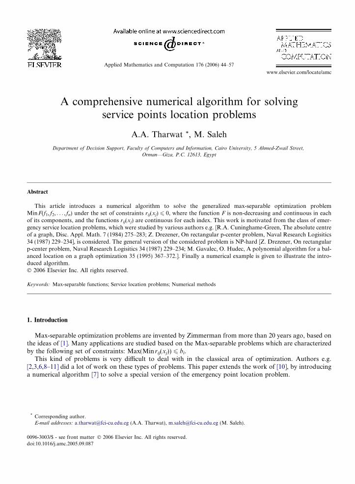
Fig. 1. Emergency points location problem.

A.A. Tharwat, M. Saleh / Applied Mathematics and Computation 176 (2006) 44–57 45

2. Problem description

Consider the following general n-center emergency points location problem, portrayed in Fig. 1. Supposethat there are m fixed points (customers) Y1,Y2, . . . ,Ym. These points have to be served from n emergencyservice centers S1,S2, . . . ,Sn. Each service center Sj has to be placed on a segment AjBj; where Aj and Bj aregiven points and the distances jAjBjj, jYiAjj, jYiBjj are known for all i 2 L = {1,2, . . . ,m} and for allj 2 N = {l, 2, . . . ,n}.

Assume that, if Yi is served by the point Sj with jAjSjj = xj, then the sever must pay the following cost

function:

rijðxjÞ ¼ minðaij þ gijðxjÞ; bij þ gijðdj � xjÞÞ;

where gij is a continuous function for all i and j, and aij, bij and dj are all constant costs assigned to the sidesYiAi, YjBj, AjBj, respectively for all i and j.

The cost ri(x1, . . . ,xn) which must be paid if Yi, i 2 L, is to be served by one of the points Sj, j 2 N, will beexpressed as follows:

riðx1; . . . xnÞ ¼ maxj2N

rijðxjÞ:

This is a ‘‘pessimistic’’ estimation of the cost.This paper suggests a method for solving an alternative location problem.

Min F ðf1ðx1Þ; . . . ; fnðxnÞÞs:t: MðaÞ; ð1Þ

where F(f1(x1), . . . , fn(xn)) is continuous and non-decreasing in each of its components, and fj’s are given con-tinuous unimodal functions, j 2 N; and

MðaÞ ¼ fx ¼ ðx1; . . . ; xnÞj max16i6m

riðxÞ 6 a 0 6 xj 6 dj; j ¼ 1; . . . ; ng: ð2Þ

In other words, F(f1(x1), . . . , fn(xn)) should be minimized over the set of such locations that are ‘‘good enough’’with respect to the chosen performance criteria ri(x) 6 a.

For example, it is needed to find such location x� ¼ ðx�1; . . . ; x�nÞ that the points S�j with j AjS�j j¼ x�j are

located as close as possible (e.g. in the Euclidian distance) to some given recommended points (pre-specifiedby the decision-maker) bSj 2 AjBj with j AjSj j¼ x̂j and at the same time ri(x*) 6 a (a is given parameter) fori = 1, . . . ,m. So the needed location x* can be found as the optimal solution of the following problem:

Min z ¼ kx� x̂k2 ¼Xn

j¼1

ðxj � x̂jÞ2 ð3Þ

s:t: x 2 MðaÞ:

46 A.A. Tharwat, M. Saleh / Applied Mathematics and Computation 176 (2006) 44–57

In the following sections, a procedure to solve a more generalized form of the optimization problem (3) will beintroduced.

3. Problem formulation

Consider the following optimization problem:

Min F ðf1ðx1Þ; . . . ; fnðxnÞÞ

s:t: maxi6j6n

rijðxjÞ 6 bi; i ¼ 1; . . . ;m

hj 6 xj 6 H j; j ¼ 1; . . . ; n; ð4Þ

where F(t1, . . . , tn) is a continuous and non-decreasing function, rij : R ! R are continuous functions, and bi,hj, Hj are given numbers, fj : R ! R are continuous unimodal functions.

Now, it is clear that problem (3) is a special case from (4); in other words, put F ðt1; . . . ; tnÞ ¼Pn

j�1tj,fjðxjÞ ¼ ðxj � x̂jÞ2, and hj = 0, Hj = dj for all i, j.

Regarding the set of inequalities in problem (4), it is known that

max16j6n

rijðxjÞ 6 bi () max16j6n

rijðxjÞ � bi 6 0:

And the functions rij(xj) � bi are continuous from the continuity of the functions rij(xj). So without loss of gen-erality, it is possible to focus on the following type of inequality rij(xj) 6 0.

4. Set of feasible solutions

Let us denote the feasible solutions of (4) by the set M, then x = (x1, . . . ,Xn) 2M implies that rij(xj) 6 0 forall i, j.

So that M ¼Qn

j¼1Mj ¼ M1 � � � � �Mn where

Mj ¼ fxj : rijðxjÞ 6 0 for all i ¼ 1; . . . ;m and xj 2 ½hj;Hj� for all j ¼ 1; . . . ; ng:

Therefore to investigate the structure of Mj under the assumptions of the functions rij(xj) for all I = 1, . . . ,m

and j = 1, . . . ,n, let us define the following sets:

V ij ¼ fxj : xj 2 ½hj;Hj� and rijðxjÞ 6 0g:

Then it is obvious that Mj ¼Tm

i¼1V ij for all j = 1, . . . ,n.Hence, some properties of the sets of Vij should investigated to clarify the structure of the feasible set M.Define the following two extreme values for each function rij(xj):

qðiÞj ¼ max rijðxjÞ : xj 2 ½hj;H j�;dðiÞj ¼ min rijðxjÞ : xj 2 ½hj;H j�:

And it is obviously remarked that there are many numerical procedures for determining the roots of each ofthe functions rij(xj) say ½xi1

j ; . . . ; xikj �.

Recalling the definition of Vij we can deduce that [8]:

1. Vij = / if dðiÞj > 0.2. Vij = [hj,Hj] if qðiÞj 6 0.

3. V ij ¼Sk

l¼1½xi1j ; x

ilþ1j �; hj 6 X il

j 6 Hj for all l = 1,2, . . . ,k.

Recalling the above information the following lemma could be proved.

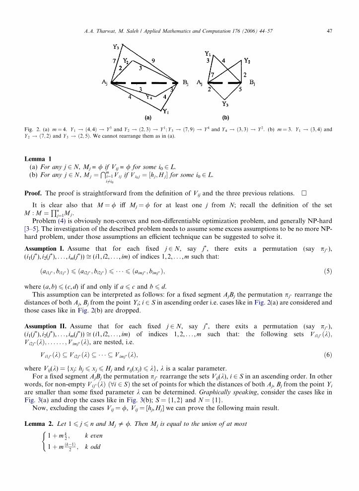
Fig. 2. (a) m = 4. Y 1 ! ð4; 4Þ ! Y 3 and Y 2 ! ð2; 3Þ ! Y 1; Y 3 ! ð7; 9Þ ! Y 4 and Y 4 ! ð3; 3Þ ! Y 2. (b) m = 3. Y 1 ! ð3; 4Þ andY 2 ! ð7; 2Þ and Y 3 ! ð2; 5Þ. We cannot rearrange them as in (a).


Lemma 1

(a) For any j 2 N, Mj = / if Vij = / for some i0 2 L.

(b) For any j 2 N , Mj ¼Tm

i¼1i6¼i0

V ij if V i0j ¼ ½hj;H j� for some i0 2 L.

Proof. The proof is straightforward from the definition of Vij and the three previous relations. h

It is clear also that M = / iff Mj = / for at least one j from N; recall the definition of the setM : M ¼

Qnj¼1Mj.

Problem (4) is obviously non-convex and non-differentiable optimization problem, and generally NP-hard[3–5]. The investigation of the described problem needs to assume some excess assumptions to be no more NP-hard problem, under those assumptions an efficient technique can be suggested to solve it.

Assumption I. Assume that for each fixed j 2 N, say j*, there exits a permutation (say pj�),(i1(j*), i2(j*), . . . , im(j*)) ffi (i1, i2, . . . , im) of indices 1,2, . . . ,m such that:

ðai1j� ; bi1j� Þ 6 ðai2j� ; bi2j� Þ 6 � � � 6 ðaimj� ; bimj� Þ; ð5Þ

where (a,b) 6 (c,d) if and only if a 6 c and b 6 d.This assumption can be interpreted as follows: for a fixed segment AjBj the permutation pj� rearrange the

distances of both Aj, Bj from the point Yi; i 2 S in ascending order i.e. cases like in Fig. 2(a) are considered andthose cases like in Fig. 2(b) are dropped.

Assumption II. Assume that for each fixed j 2 N, say j*, there exits a permutation (say pj�),(i1(j*), i2(j*), . . . , im(j*)) ffi (i1, i2, . . . , im) of indices 1,2, . . . ,m such that: the following sets V i1j� ðkÞ;V i2j� ðkÞ; . . . . . . ; V imj� ðkÞ, are nested, i.e.

V i1j� ðkÞ � V i2j� ðkÞ � � � � � V imj� ðkÞ; ð6Þ

where Vij(k) = {xj: hj 6 xj 6 Hj and rij(xj) 6 k}, k is a scalar parameter.For a fixed segment AjBj the permutation pj� rearrange the sets Vij(k), i 2 S in an ascending order. In other

words, for non-empty V ij� ðkÞ ð8i 2 SÞ the set of points for which the distances of both Aj, Bj from the point Yi

are smaller than some fixed parameter k can be determined. Graphically speaking, consider the cases like inFig. 3(a) and drop the cases like in Fig. 3(b); S = {1,2} and N = {1}.

Now, excluding the cases Vij = /, Vij = [hj,Hj] we can prove the following main result.

Lemma 2. Let 1 6 j 6 n and Mj 5 /. Then Mj is equal to the union of at most

1þ m k2; k even

1þ m ðk�1Þ2; k odd

(

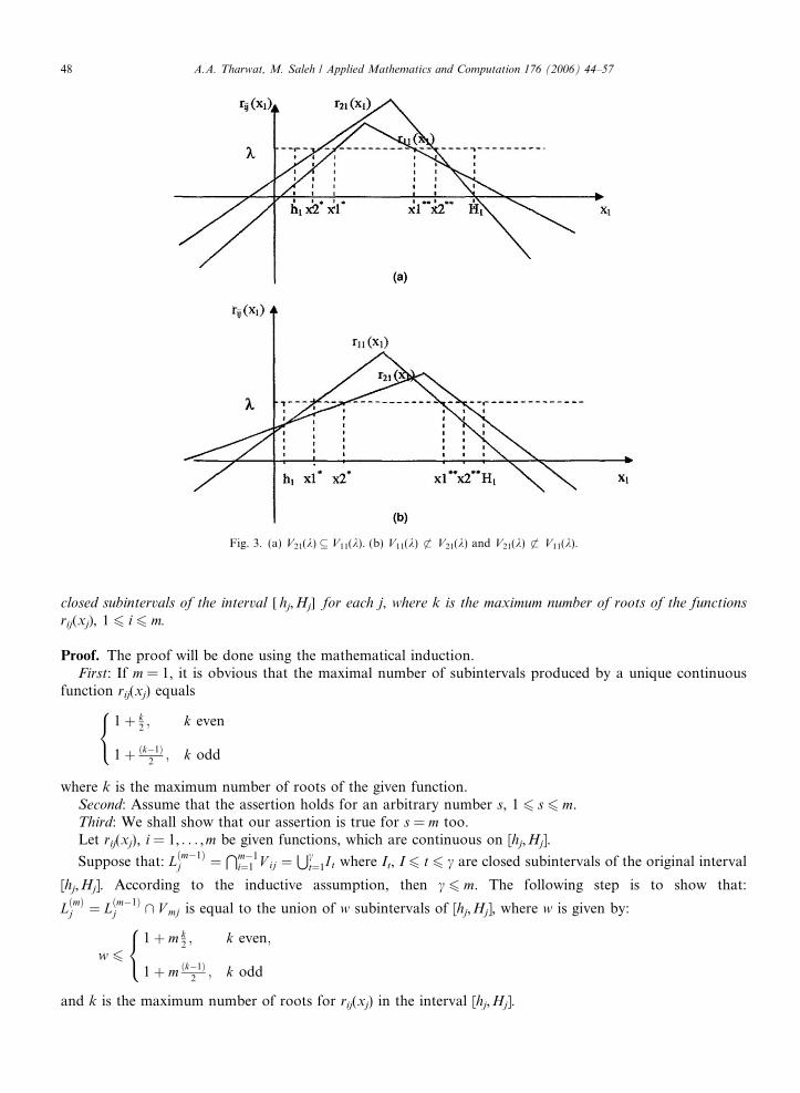
Fig. 3. (a) V21(k) � V11(k). (b) V11(k) 6 V21(k) and V21(k) 6 V11(k).


closed subintervals of the interval [hj,Hj] for each j, where k is the maximum number of roots of the functions

rij(xj), 1 6 i 6 m.

Proof. The proof will be done using the mathematical induction.First: If m = 1, it is obvious that the maximal number of subintervals produced by a unique continuous

function rij(xj) equals

1þ k2; k even

1þ ðk�1Þ2; k odd

8<:
where k is the maximum number of roots of the given function.
Second: Assume that the assertion holds for an arbitrary number s, 1 6 s 6 m.Third: We shall show that our assertion is true for s = m too.Let rij(xj), i = 1, . . . ,m be given functions, which are continuous on [hj,Hj].

Suppose that: Lðm�1Þj ¼

Tm�1i¼1 V ij ¼

Sct¼1I t where It, I 6 t 6 c are closed subintervals of the original interval

[hj,Hj]. According to the inductive assumption, then c 6 m. The following step is to show that:

LðmÞj ¼ Lðm�1Þj \ V mj is equal to the union of w subintervals of [hj,Hj], where w is given by:

w 61þ m k

2; k even;

1þ m ðk�1Þ2; k odd

8<:
and k is the maximum number of roots for rij(xj) in the interval [hj,Hj].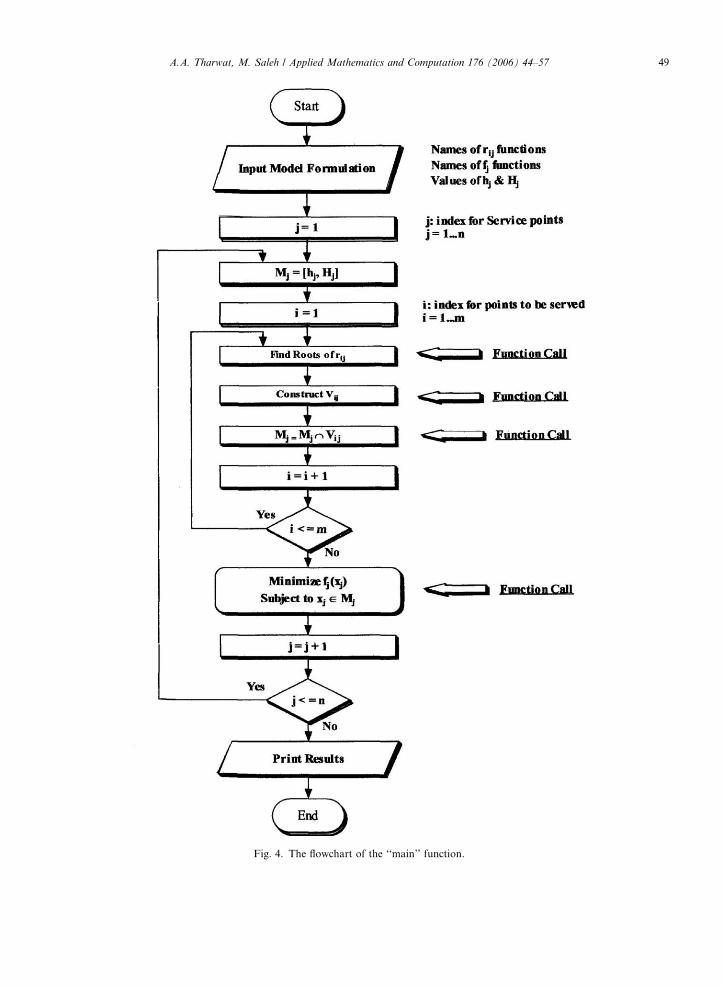

Fig. 4. The flowchart of the ‘‘main’’ function.


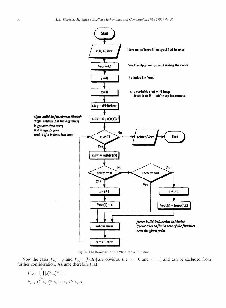
Fig. 5. The flowchart of the ‘‘find roots’’ function.


Now the cases Vmj = / and Vmj = [hj,Hj] are obvious, (i.e. w = 0 and w = c) and can be excluded fromfurther consideration. Assume therefore that:

V mj ¼[k‘¼1

xm‘j ; x

m‘þ1j

� �;

hj 6 xm16 xm2

6 � � � 6 xmk6 Hj:
j j j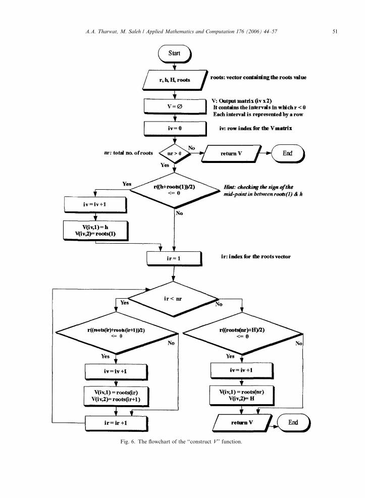

Fig. 6. The flowchart of the ‘‘construct V’’ function.


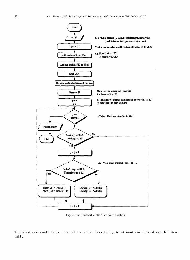
Fig. 7. The flowchart of the ‘‘intersect’’ function.


The worst case could happen that all the above roots belong to at most one interval say the inter-val It0.

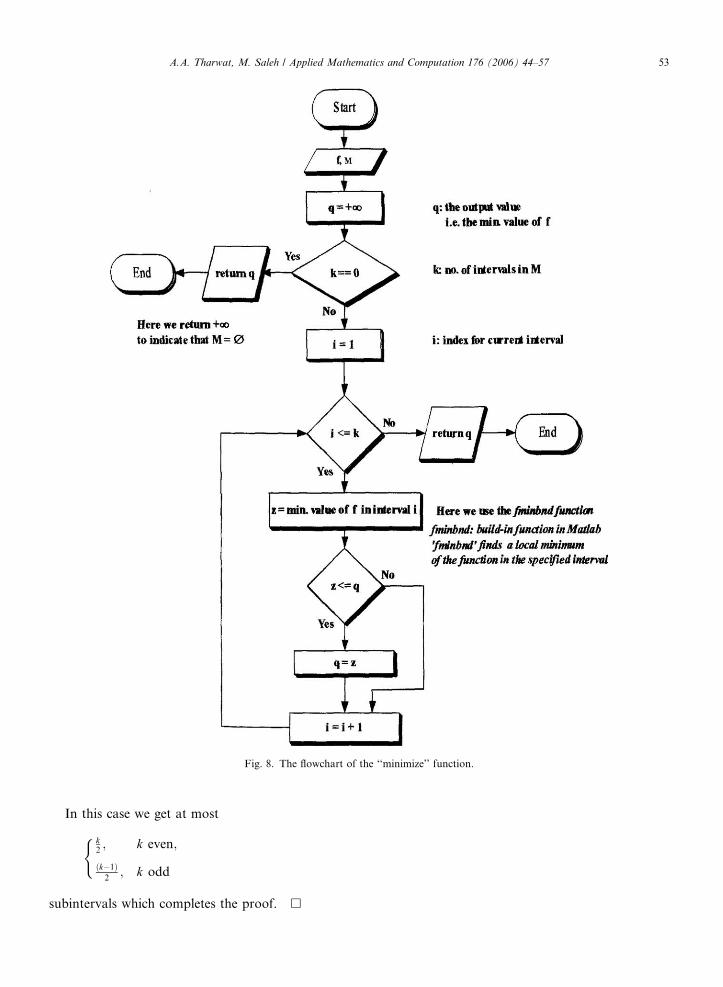
Fig. 8. The flowchart of the ‘‘minimize’’ function.


In this case we get at most

k2; k even;

ðk�1Þ2; k odd

(

subintervals which completes the proof. h


In the following we shall introduce the numerical algorithm to solve problem (4) taking into considerationthe two Assumptions I and II and the result of Lemma 2.

5. Algorithm

Fig. 4 outlines the main algorithm introduced in this paper (which was implemented in using Matlab soft-ware). Basically the algorithm consists of a double loops structure. The outer-loop scans all the given servicepoints (j = 1, . . . ,n); while in the inner-loop all the points to be served (customers) are scanned (i = 1, . . . ,m).

Before entering the inner-loop Mj is set to [hj,Hj].The inner-loop carries out the following steps:

1. Find the roots of rij.2. Construct the associated Vij intervals based on the roots of rij.3. Update Mj by intersecting it with the newly identified Vij.

Below, we will briefly explain each step in the inner loop.First, the idea of the ‘‘find roots’’ function—as illustrated in Fig. 5 (flowchart of the function)—is to scan all

the interval [h,H] by incrementally moving (with a very small step specified by the user) from h to H. If a smallincremental step changed the sign of the function r, then a root must exist in this small region. Here, the build-in Matlab ‘sign’ function is used to indicate the sign of a given input real number. Moreover, the build-in Mat-lab ‘fzero’ function is used to identify a root of an input function near a pre-specified input point, ‘fzero’ relieson the presence of an interval where the function values of the interval endpoints differ in sign, then searchesthat interval for a zero.

Second, the idea of the ‘‘construct V’’ function—as illustrated in Fig. 6 (flowchart of the function)—is tofind the various intervals, where r is less than zero. At the beginning, mid point between h and first root of r ischecked; if the value of r at this point is less than zero, then [h, first root of r] 2 V. Similarly, the mid pointsbetween each two successive roots are checked. And at the end, the mid point between the last root of r and H

is checked.Third, the idea of the ‘‘intersect’’ function—as illustrated in Fig. 7 (flowchart of the function)—is to find the

various intervals, which belong to both Mj and Vij. Initially, all the end points (nodes) of all intervals of Mj

and Vij are stored in a single vector. Then this vector is sorted, and the redundant points are removed (if theyexist). Then for each node, in this vector, the following procedure is carried: First, check that the node belongsto both Mj and Vij. If this is true, then further check that the value of this node + eps. (very small no. around2e�16) belongs to both Mj and Vij. If this true, then the interval, which starts from this node, and ends at thenext successive node, must belong to both Mj and Vij, otherwise only this node belongs to both Mj and Vij.

After completing the inner-loop, the final correct Mj is obtained. Consequently, the next step, in the outer-loop is to find the minimum fj, s.t. xj 2Mj. This step is illustrated in Fig. 8 (flowchart of the minimize func-tion). The idea of this step is to find the local minimum in each interval of Mj, using the built-in Matlab func-tion ‘fminbnd’ (which finds a local minimum of the input function in a specified continuous input interval).Then the smallest local minimum is selected as the point which minimizes fj, s.t. xj 2Mj. Finally, after theouter-loop finishes, the results of the algorithm are exported to an excel file.

6. Numerical example

Assume that there are three customers Y1, Y2 and Y3 (j = 1,2,3), and those customers have to be servedfrom two emergency service centers S1 and S2 (i = 1,2). Now the question is: where we should locate each ser-vice center Sj on the corresponding segment AjBj, that to minimize the total service cost.

Given that the decision-maker has recommend the position (6, 6) for the two service centers, in other wordsthe two components of the objective function (to be minimized) are the following continuous and unimodalfunctions:

f ðx1Þ ¼ ðx1 � 6Þ2 and f ðx2Þ ¼ ðx2 � 6Þ2:


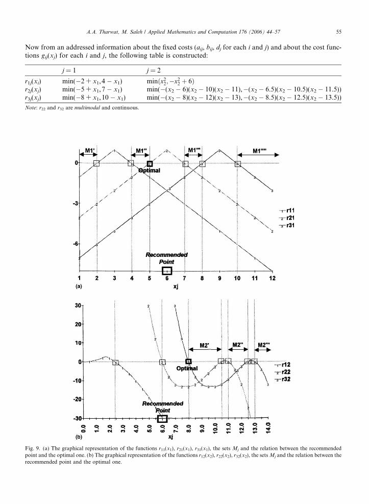
Now from an addressed information about the fixed costs (aij, bij, dj for each i and j) and about the cost func-tions gij(xj) for each i and j, the following table is constructed:

Fig. 9. (a) Thepoint and the oprecommended p

j = 1

graphical representation of the functimal one. (b) The graphical represenoint and the optimal one.

j = 2

r1j(xi)
min(�2 + x1,4 � x1) minðx22;�x2
2 þ 6Þ
r2j(xj) min(�5 + x1,7 � x1) min(�(x2 � 6)(x2 � 10)(x2 � 11),�(x2 � 6.5)(x2 � 10.5)(x2 � 11.5)) r3j(xj) min(�8 + x1,10 � x1) min(�(x2 � 8)(x2 � 12)(x2 � 13),�(x2 � 8.5)(x2 � 12.5)(x2 � 13.5))
Note: r22 and r32 are multimodal and continuous.

tions r11(x1), r21(x1), r31(x1), the sets Mj and the relation between the recommendedtation of the functions r12(x2), r22(x2), r32(x2), the sets Mj and the relation between the


Assuming that the recommended intervals for the decision variables x1 and x2 are given by the inequalities1 6 x1 6 12 and 0 6 x2 6 14, hence the intersection of the functions rij(xj) i = 1 . . . , 3, j = 1,2 can be identified,as illustrated in Fig. 9(a) and (b).

Solution

The results of the numerical algorithm are as follows:

First: Roots of rij

j = 1
j = 2
r1j(xj)
[2, 4] [0,2.45] r2j(xj) [5, 7] [6,10.5, 11] r3j(xj) [8, 10] [8,12.5, 13]
Second: Vij

j = 1
j = 2
V1j
[1,2] [ [4, 12] [0,0] [ [2.45,14] V2j [1,5] [ [7, 12] [6,10.5] [ [11, 14] V3j [1,8] [ [10, 12] [8,12.5] [ [13, 14]
Third: Mj

M1 ¼ ½1; 2� [ ½4; 5� [ ½7; 8� [ ½10; 12�;

M2 ¼ ½8; 10:5� [ ½11; 12:5� [ ½13; 14�:

Fourth: The optimal solution: x* = (5,8), i.e. the suggested location for the two service center is (5, 8).Fifth: The minimum value of the objective function F(x) is equal to

f1ðx�1Þ þ f2ðx�2Þ ¼ 1þ 4 ¼ 5:

7. Conclusions

In this article a modified problem from the class of emergency service location problems, which were stud-ied in [5] is considered. Motivated by the fact that in many real life situations the formulated problem isaccompanied with multimodal cost functions; hence an extended algorithm is introduced (in spirit of [10])to deal with such special version of the location problem.

In this version of the algorithm there is only one solution could be identified, even if there are several opti-mal alternative solutions. However, in future research, the algorithm can be modified to identify all the multi-ple optimal solutions. Also as an extension of this work, weights can be considered to differentiate between themain two paths from the service point to the customers.

References

[1] R.A. Cuninghame-Green, Mini–Max Algebra, Lecture Notes in Economics and Mathematical Systems, Springer Verlag, 1979.[2] R.A. Cuninghame-Green, The absolute centre of a graph, Disc. Appl. Math. 7 (1984) 275–283.[3] Z. Drezener, On rectangular p-center problem, Naval Res. Logist. 34 (1987) 229–234.[4] O. Hudec, An alternative p-centre problem, in: Proceedings of ‘‘Optimization’’ Conference, Eisenach, 1989.[5] O. Hudec, K. Zimmermann, Biobjective centre-balance graph location model, Optimization 45 (1999) 107–115.[6] A. Tharwat, K. Zimmermann, Optimal choice of parameters in a machine time scheduling problems, in: Proceedings of

‘‘Mathematical Methods in Economics ad Industry’’ Conference, Liberec, Czech Republic, 1968, pp. 107–112.


[7] W. Press, B. Flannery, S. Teukolsky, W. Vetterling, Numerical Recipes in C: The Art of Scientific Computing, second ed., CambridgeUniversity Press, 1992.

[8] A. Tharwat, A generalized algorithm to solve emergency service location-problem, in: Proceedings of ‘‘Mathematical Methods inEconomics’’ International Conference, Prague, Czech Republic, 2000.

[9] A. Tharwat, K. Zimmermann, A difference scalarization technique to solve bi-criteria location problem, in: Proceedings of the FirstInternational Conference on Informatics ad Systems, Faculty of Computer ad Information, Cairo University, 2002.

[10] K. Zimmermann, Max-Separable optimization problems with uni-modal functions, Eknomicko-matematicky obzor 27 (2) (1991)159–169.

[11] K. Zimmermann, A parametric approach to solving one location problem with additional constraints, in: Proceedings ‘‘ParametricOptimization and Related Topics III’’, Approximation and Optimization, Verlag Peter Lang, 1993, pp. 557–568.

A comprehensive numerical algorithm for solving service points location problems

Documents