Master Thesis Software Engineering Thesis no: MSE-2011-66 September 2011 o A Comprehensive Evaluation of Conversion Approaches for Different Function Points Javad Mohammadian Amiri Venkata Vinod Kumar Padmanabhuni School of Computing Blekinge Institute of Technology SE-371 79 Karlskrona Sweden

Welcome message from author
This document is posted to help you gain knowledge. Please leave a comment to let me know what you think about it! Share it to your friends and learn new things together.
Transcript
Master Thesis
Software Engineering
Thesis no: MSE-2011-66
September 2011 o
School of Computing
Blekinge Institute of Technology
SE-371 79 Karlskrona
Sweden
A Comprehensive Evaluation of
Conversion Approaches for Different
Function Points
Javad Mohammadian Amiri
Venkata Vinod Kumar Padmanabhuni
School of Computing
Blekinge Institute of Technology
SE-371 79 Karlskrona
Sweden

This thesis is submitted to the School of Computing at Blekinge Institute of Technology in
partial fulfillment of the requirements for the degree of Master of Science in Software
Engineering. The thesis is equivalent to 20 weeks of full time studies.
Contact Information:
Author(s):
Javad Mohammadian Amiri
E-mail:[email protected]
Venkata Vinod Kumar Padmanabhuni
E-mail:[email protected]
University advisor(s): Dr. CigdemGencel
School of Computing, BTH
School of Computing
Blekinge Institute of Technology
SE-371 79 Karlskrona
Sweden
Internet : www.bth.se/com Phone : +46 455 38 50 00
Fax : +46 455 38 50 57
ii
ABSTRACT
Context: Software cost and effort estimation are important activities for planning and estimation of
software projects. One major player for cost and effort estimation is functional size of software which
can be measured in variety of methods. Having several methods for measuring one entity, converting
outputs of these methods becomes important.
Objectives: In this study we investigate different techniques that have been proposed for conversion
between different Functional Size Measurement (FSM) techniques. We addressed conceptual
similarities and differences between methods, empirical approaches proposed for conversion,
evaluation of the proposed approaches and improvement opportunities that are available for current
approaches. Finally, we proposed a new conversion model based on accumulated data.
Methods: We conducted a systematic literature review for investigating the similarities and
differences between FSM methods and proposed approaches for conversion. We also identified some
improvement opportunities for the current conversion approaches. Sources for articles were IEEE
Xplore, Engineering Village, Science Direct, ISI, and Scopus. We also performed snowball sampling
to decrease chance of missing any relevant papers. We also evaluated the existing models for
conversion after merging the data from publicly available datasets. By bringing suggestions for
improvement, we developed a new model and then validated it.
Results: Conceptual similarities and differences between methods are presented along with all
methods and models that exist for conversion between different FSM methods. We also came with
three major contributions for existing empirical methods; for one existing method (piecewise linear
regression) we used a systematic and rigorous way of finding discontinuity point. We also evaluated
several existing models to test their reliability based on a merged dataset, and finally we accumulated
all data from literature in order to find the nature of relation between IFPUG and COSMIC using
LOESS regression technique.
Conclusions: We concluded that many concepts used by different FSM methods are common which
enable conversion. In addition statistical results show that the proposed approach to enhance
piecewise linear regression model slightly increases model’s test results. Even this small improvement
can affect projects’ cost largely. Results of evaluation of models show that it is not possible to say
which method can predict unseen data better than others and it depends on the concerns of practitioner
that which model should be used. And finally accumulated data confirms that empirical relation
between IFPUG and COSMIC is not linear and can be presented by two separate lines better than
other models. Also we noted that unlike COSMIC manual’s claim that discontinuity point should be
around 200 FP, in merged dataset discontinuity point is around 300 to 400. Finally we proposed a new
conversion approach using systematic approach and piecewise linear regression. By testing on new
data, this model shows improvement in MMRE and Pred(25).
Keywords: Functional Size Measurement (FSM),
Conversion, Systematic Literature Review, Regression
Analysis

iii
ACKNOWLEDGMENT
First and foremost I want to thank Allah almighty for giving strengths and power to me
to finish this thesis. May he make us and all humanity happy by returning, his long-
awaited representative on the earth, his Excellency Mahdi -peace be upon him- for
bringing justice and peace to the world of wrongdoing, injustice and oppression.
Next I express my gratitude to my family i.e. father, mother and wife. I thank my
parents for their sincere and constant support during all stages of my life. I thank my
wife for being patient and supporting during all this thesis work. I never forget their
encouragement and support during all days of my life.
Also I should thank my thesis partner Vinod for his always smiling face and helping
hand. Without his patience many problems couldn‘t be solved easily.
Last but not least I thank Dr. Cigdem Gencel for her useful and helpful guidance
during all stages of our work.
- Javad
Firstly it's an honor to thank our supervisor Dr. Cigdem Gencel for her supervision,
advice and guidance from start of this thesis. She supported us in developing
understanding of the subject and providing us feedback with great patience. We also
thank to the BTH library members for their support during string formulation and
database search.
I would like to thank my thesis partner Javad Amiri for his dedication, help and effort
he has put in this thesis along with me, without him this thesis would be impossible. It
was a pleasure to work with him as it has been an inspiring, often exciting, sometimes
challenging, but always interesting experience.
I owe my deepest gratitude to my family members for their encouragement in pursuing
my master‘s degree despite all obstacles encountered on the way. I would also like to
thank them for the financial support that they have so readily provided.
I thank my home university Andhra University, India for providing me an opportunity
in doing this Double Diploma Program with BTH, Sweden. Finally I would like to
thank all my friends and seniors for their support and encouragement during my stay in
Sweden.
- Vinod Kumar
iv
LIST OF TABLES Table 1. FSM methods, their ISO certification number and their unit of measure ......... 9 Table 2. Complexity matrix of EI, EO and EQ [14] ......................................................... 15 Table 3. Complexity matrix of ILF and EIF [14] ............................................................. 15 Table 4. Keywords for Research question 1 ..................................................................... 24 Table 5. Keywords for Research question 2 ..................................................................... 25 Table 6. Databases used in the SLR .................................................................................. 25 Table 7. Quality Assessment Checklist.............................................................................. 26 Table 8. Data Extraction Form .......................................................................................... 27 Table 9. Search Strings for systematic review .................................................................. 28 Table 10. List of articles selected for RQ1 ........................................................................ 29 Table 11. List of articles selected for RQ2 ........................................................................ 29 Table 12. Search result for RQ1 and RQ2 ........................................................................ 31 Table 13. Calculated Kappa coefficient for each database .............................................. 32 Table 14. Articles selected from databases and snowball sampling ................................ 32 Table 15. List of articles included for primary study ....................................................... 33 Table 16. Results of Quality Assessment Criteria ............................................................ 35 Table 17. Mapping of studies quality groups .................................................................... 35 Table 18. Articles, methods discussed in each and type of relation that they discuss .... 37 Table 19. Quick summary of articles regarding conceptual similarities and differences
...................................................................................................................................... 41 Table 20. Common concepts between different FSM methods ....................................... 42 Table 21. Comparison of constituent parts of IFPUG, Mark II and COSMIC FSM
methods (originally appeared in [17]) ....................................................................... 44 Table 22. Conversion formulas between BFCs of IFPUG and COSMIC FFP ............... 48 Table 23. Linear models for FPA-TX and COSMIC FFP ............................................... 49 Table 24. Linear Regression formulas of COSMIC and IFPUG or NESMA functional
sizes .............................................................................................................................. 51 Table 25. Relationship between IFPUG and COSMIC using OLS, LMS regressions... 52 Table 26. Precision of OLS and LMS regression on respective datasets ........................ 52 Table 27. Piecewise Linear Conversion without removing outliers for IFPUG and
COSMIC ...................................................................................................................... 54 Table 28. piecewise regression models with removing outliers for IFPUG and COSMIC
conversions .................................................................................................................. 55 Table 29. Correlation between FP and CFP BFC’s ......................................................... 56 Table 30. Relationship between IFPUG and COSMIC using log-log transformation ... 57 Table 31. Comparison of Systematic Approach (SA) and Lavazza and Morasca’s
(L&M) work for finding discontinuity point in a dataset ........................................ 66 Table 32. Codes for Datasets .............................................................................................. 70 Table 33. Codes for Authors .............................................................................................. 70 Table 34. Codes for methods .............................................................................................. 70 Table 35. Statistical Analysis Results of Sogeti data set 2006 .......................................... 71 Table 36. Statistical Analysis Results of Rabobank dataset ............................................ 73 Table 37. Statistical Analysis Results of Desharnais 2006 Dataset .................................. 75 Table 38. Statistical Analysis Results of Cuadrado-Gallaego et al. 2007 dataset ........... 77 Table 39. Statistical Analysis Results of warehouse portfolio dataset ............................ 79 Table 40. Statistical Analysis Results of Desharnais 2005 dataset .................................. 80 Table 41. Statistical Analysis Results of jjcg06 dataset .................................................... 81 Table 42. Statistical Analysis Results of jjcg07 dataset .................................................... 83 Table 43. Statistical Analysis Results of jjcg0607 dataset ................................................ 85
Table-A 1. Search strategy for RQ1 ................................................................................ 102 Table-A 2. Search strategy for RQ2 ................................................................................ 105
v
Table-B 1. Mark II FP data ............................................................................................. 107 Table-B 2. FP Albrecht Data ........................................................................................... 108 Table-B 3. FSM Measures of warehouse management portfolio .................................. 109 Table-B 4. Rabobank Sizing Results ............................................................................... 109 Table-B 5. Desharnais 2005 dataset................................................................................. 109 Table-B 6. Desharnais 2006 dataset................................................................................. 110 Table-B 7. Projects Measurement Results ...................................................................... 110 Table-B 8. Military Inventory Management project measures ..................................... 111 Table-B 9. Sogeti dataset .................................................................................................. 112 Table-B 10. jjcg06 Dataset ............................................................................................... 113 Table-B 11. jjcg07 Dataset ............................................................................................... 113 Table-B 12. Simple Locator dataset ................................................................................ 114 Table-B 13. PCGeek dataset ............................................................................................ 114 Table-B 14. Avionics Management system dataset ........................................................ 114 Table-B 15. Merged Dataset ............................................................................................ 115 Table-B 16. Conversion model datasets .......................................................................... 116
Table-C 1. Formulas derived from applying systematic piecewise approach .............. 117 Table-C 2. Formulas with applying log-log transformation on datasets ...................... 118
vi
LIST OF FIGURES Figure 1. Evolution of FSM methods based on the time (Figure from Cuadrado-Gallego
et al. [8]) ....................................................................................................................... 10 Figure 2. IFPUG FPA measurement process .................................................................... 14 Figure 3. Application user view in IFPUG FPA (originally from Galorath and Evans
[27]) .............................................................................................................................. 16 Figure 4. Application view in COSMIC measurement process ....................................... 17 Figure 5. Research methodology used to answer RQs. .................................................... 20 Figure 6. The process of selecting papers for SLR ........................................................... 30 Figure 7. The process of snowball sampling ..................................................................... 33 Figure 8. Distribution of articles based on source type .................................................... 36 Figure 9. Distribution of articles based on identified categories ..................................... 37 Figure 10. Number of papers in each category according to year of publication .......... 38 Figure 11. Number of data points per data set ................................................................. 39 Figure 12. Abstract view of measurement steps in all FSM methods ............................. 40 Figure 13. categorization of conversion between COSMIC and IFPUG (or NESMA) .. 47 Figure 14. Categorization of conversion between IFPUG and Mk II ............................. 58 Figure 15. Scatter plot of Rabobank dataset with an OLS regression line ..................... 62 Figure 16. Scatterplot of Rabobank dataset with two linear lines; less than 200 FP (Blue
line) and bigger than 200 FP (Red line) ..................................................................... 62 Figure 17. Scatterplot of Rabobank dataset with LMS regression line .......................... 63 Figure 18. Scatterplot of Rabobank dataset with regression equation after log-log
transformation ............................................................................................................ 63 Figure 19. Flow chart for Systematic Approach............................................................... 65 Figure 20. Scatterplot of Rabobank dataset with LOESS line ........................................ 67 Figure 21. Preparing Test Dataset points for Cuadrado 2007 models ............................ 68 Figure 22. Boxplots for ‘e’ estimates of Sogeti dataset 2006 ............................................ 72 Figure 23. Boxplots for ‘z’ estimates of Sogeti dataset 2006 ............................................ 73 Figure 24. Boxplots for ‘e’ estimates of Rabobank dataset ............................................. 74 Figure 25. Boxplots for ‘z’ estimates of Rabobank dataset ............................................. 75 Figure 26. Boxplots for ‘e’ estimates of Desharnais 2006 Dataset ................................... 76 Figure 27. Boxplots for ‘z’ estimates of Desharnais 2006 Dataset ................................... 77 Figure 28. Boxplots for ‘e’ estimates of Cuadrado-Gallaego et al. 2007 dataset ............ 78 Figure 29. Boxplots for ‘z’ estimates of Cuadrado-Gallaego et al. 2007 dataset ............ 78 Figure 30. Boxplots for ‘e’ estimates of warehouse portfolio dataset ............................. 79 Figure 31. Boxplots for ‘z’ estimates of warehouse portfolio dataset ............................. 80 Figure 32. Boxplots for ‘e’ estimates of Desharnais 2005 dataset ................................... 81 Figure 33. Boxplots for ‘z’ estimates of Desharnais 2005 dataset ................................... 81 Figure 34. Boxplots for ‘e’ estimates of jjcg06 dataset ..................................................... 82 Figure 35. Boxplots for ‘z’ estimates of jjcg06 dataset ..................................................... 83 Figure 36. Boxplots for ‘e’ estimates of jjcg07 dataset ..................................................... 84 Figure 37. Boxplots for ‘z’ estimates of jjcg07 dataset ..................................................... 84 Figure 38. Boxplots for ‘e’ estimates of jjcg0607 dataset ................................................. 86 Figure 39. Boxplots for ‘z’ estimates of jjcg0607 dataset ................................................. 86 Figure 40. Merged dataset with a smoothing line using LOESS ..................................... 87 Figure 41. Pictorial representation of how the model was built ...................................... 89
vii
CONTENTS ABSTRACT ..................................................................................................................................... II
ACKNOWLEDGMENT ............................................................................................................... III
LIST OF TABLES .......................................................................................................................... IV
LIST OF FIGURES ........................................................................................................................ VI
CONTENTS .................................................................................................................................. VII
1 INTRODUCTION .................................................................................................................... 9
1.1 PURPOSE STATEMENT ....................................................................................................... 11 1.2 AIMS AND OBJECTIVES ..................................................................................................... 11 1.3 RESEARCH QUESTIONS ..................................................................................................... 11 1.4 THESIS OUTLINE ............................................................................................................... 11
2 BACKGROUND .................................................................................................................... 13
2.1 ISO 14143 STANDARD ON FSM ........................................................................................ 13 2.2 IFPUG FPA ..................................................................................................................... 14 2.3 COSMIC ......................................................................................................................... 16 2.4 MARK II FPA ................................................................................................................... 17
3 RESEARCH METHODOLOGY .......................................................................................... 19
3.1 SYSTEMATIC LITERATURE REVIEW ................................................................................... 19 3.1.1 Snowball Sampling ..................................................................................................... 21
3.2 DATA ANALYSIS/SYNTHESIS ............................................................................................ 21 3.2.1 Narrative Analysis ...................................................................................................... 21 3.2.2 Comparative Analysis ................................................................................................. 21 3.2.3 Statistical Analysis ...................................................................................................... 21 3.2.4 Alternative Methods .................................................................................................... 21
4 SYSTEMATIC LITERATURE REVIEW ............................................................................ 23
4.1 PLANNING ........................................................................................................................ 23 4.1.1 The Need for a Systematic Review .............................................................................. 23 4.1.2 Specifying Research Questions ................................................................................... 23 4.1.3 Defining Keywords ..................................................................................................... 23 4.1.4 Search for Studies ....................................................................................................... 25 4.1.5 Study Selection Criteria .............................................................................................. 26 4.1.6 Study Selection Procedure .......................................................................................... 26 4.1.7 Study Quality Assessment ........................................................................................... 26 4.1.8 Data Extraction .......................................................................................................... 27 4.1.9 Data Analysis and Synthesis ....................................................................................... 28 4.1.10 Pilot Study .............................................................................................................. 28
4.2 CONDUCTING THE REVIEW ............................................................................................... 28 4.2.1 Identification of Research .......................................................................................... 28 4.2.2 Articles Selection Criteria ........................................................................................... 28 4.2.3 Calculation of Kappa Coefficient ............................................................................... 31 4.2.4 Snowball Sampling ..................................................................................................... 32 4.2.5 Selected Articles for Study .......................................................................................... 32 4.2.6 Study Quality Assessment ........................................................................................... 35
4.3 REPORTING THE REVIEW RESULTS .................................................................................... 36 4.3.1 General Information on Articles................................................................................. 36 4.3.2 Data Extraction Results .............................................................................................. 37
4.4 DATA ANALYSIS & RESULTS ............................................................................................ 39 4.4.1 Conceptual Similarities and Differences .................................................................... 39
4.4.1.1 Collected Data on Similarities and Differences ...................................................................... 41 4.4.1.2 Similarity and Difference in Basic Definitions ....................................................................... 42 4.4.1.3 Similarity and Difference in Constituent Parts........................................................................ 42 4.4.1.4 Discussion on Similarities and Differences ............................................................................. 42

viii
4.4.1.5 Sources of differences between methods................................................................................. 45 4.4.2 Conversion Approaches of FSM methods................................................................... 46
4.4.2.1 Conversion between COSMIC and IFPUG (or NESMA) ...................................................... 47 A. Theoretical models ...................................................................................................................... 47 B. Statistically-driven models ......................................................................................................... 49
4.4.2.2 Conversion between IFPUG and Mk II ................................................................................... 57 A. Theoretical models ........................................................................................................................... 57
5 RELIABILITY OF CONVERSION APPROACHES .......................................................... 60
5.1 REGRESSION TECHNIQUES ALREADY USED IN CONVERSION .............................................. 60 5.1.1 Linear Regression ....................................................................................................... 60 5.1.2 Piecewise Linear Regression ...................................................................................... 60 5.1.3 Robust Regression Models .......................................................................................... 61 5.1.4 Non-linear Models ...................................................................................................... 61
5.2 AN IMPROVEMENT SUGGESTION FOR SYSTEMATICALLY HANDLING DISCONTINUITY POINT
IN COSMIC-IFPUG RELATIONSHIP .............................................................................................. 64 5.2.1 Piecewise OLS with Log-log Transformation ............................................................. 66 5.2.2 Nearest Neighborhood Linear Regression (AKA LOESS or LOWESS) ..................... 66
5.3 MERGING PUBLICLY AVAILABLE DATASETS FOR EVALUATION ......................................... 66 5.4 EVALUATION OF CONVERSION APPROACHES..................................................................... 68
5.4.1 Criteria for Evaluation ............................................................................................... 68 5.4.2 Evaluation Results ...................................................................................................... 69
5.4.2.1 Van Heeringen 2007 (Sogeti dataset 2006) ............................................................................. 71 5.4.2.2 Vogelezang & Lesterhuis 2003 (Rabobank) ........................................................................... 73 5.4.2.3 Desharnais et al. 2006 (Desharnais 2006 dataset) ................................................................... 75 5.4.2.4 Cuadrado-Gallaego et al. 2007 ................................................................................................ 77 5.4.2.5 Fetcke 1999 (warehouse portfolio) .......................................................................................... 79 5.4.2.6 Abran et al. 2005 (Desharnais 2005 dataset) ........................................................................... 80 5.4.2.7 Cuadrado-Gallaego et al. 2008 (jjcg06) .................................................................................. 81 5.4.2.8 Cuadrado-Gallaego et al. 2008 (jjcg07) .................................................................................. 83 5.4.2.9 Cuadrado-Gallaego et al. 2010 (jjcg0607) .............................................................................. 85
6 A NEW CONVERSION MODEL ......................................................................................... 87
6.1 RELATION BETWEEN IFPUG AND COSMIC BY APPLYING LOESS .................................... 87 6.2 APPROACH FOR BUILDING NEW MODEL............................................................................ 88
7 DISCUSSION ......................................................................................................................... 90
7.1 IMPROVEMENT SUGGESTION FOR HANDLING DISCONTINUITY POINT SYSTEMATICALLY .... 90 7.2 EVALUATION OF DATASETS .............................................................................................. 90 7.3 STUDY OF MERGED DATASET AND A NEW CONVERSION MODEL ...................................... 91
8 VALIDITY THREATS .......................................................................................................... 92
8.1 INTERNAL VALIDITY ........................................................................................................ 92 8.2 CONSTRUCT VALIDITY ..................................................................................................... 92 8.3 CONCLUSION VALIDITY .................................................................................................... 93 8.4 EXTERNAL VALIDITY ....................................................................................................... 93
9 CONCLUSION AND FUTURE WORK ............................................................................... 94
9.1 CONCLUSION .................................................................................................................... 94 9.2 FUTURE WORK ................................................................................................................. 95
REFERENCES ............................................................................................................................... 96
APPENDIX A ............................................................................................................................... 102
APPENDIX B ................................................................................................................................ 107
APPENDIX C ............................................................................................................................... 117
GLOSSARY .................................................................................................................................. 122

9
1 INTRODUCTION Measurement plays an important role in managing and conducting software projects. During different phases
of software development project, different measures come into play. Especially in the early phases of a
project life cycle, concerns regarding reliable software effort and cost estimation and project planning arise
[1]. Effort estimation may influence schedule, cost, scope and quality [2].
In order to make reliable estimates several methods are proposed such as parametric models, expert based
techniques, learning oriented techniques, dynamics based models, regression based models, and composite-
bayesian technique for integrating expertise and regression based models [3]. Many effort estimating models
and tools, such as COCOMO II [4] use functional size of the product as their major input [5].
Functional Size Measurement (FSM) methods measure software size based on the amount of functionality to
be delivered to the user regardless of implementation details [1]. Measuring software based on the functional
size started by Albrecht [6] in IBM and later that method was polished by Albrecht and Gaffney [7]. At a first
glance the method had several benefits. It was a way to measure size of the software quite early in the project
i.e. when only software requirements specification is available. Another aspect was that all measurements are
from end user‘s point of view which allows non-technical stakeholders gain some knowledge and information
about size of project [8]. In 1984 International Function Point User Group (IFPUG) promoted the Albrecht‘s
Function Point by setting standards and documenting the method under the name of IFPUG. Since then
IFPUG is publishing Counting Practice Manuals for the IFPUG Function Point Analysis (FPA) method [9].
Several other methods for measuring the functional size of software have been developed. MARK II FPA
[10], Netherlands Software Metrics Association (NESMA) [11], Finnish Software Metrics Association
(FiSMA) [12], and Common Software Metrics International Consortium (COSMIC) [13] are well-known
methods that all are accepted by ISO as FSM standard [8]. ISO certification number and the unit of measure
for each method are presented in Table 1. It is worth mentioning that in this table unit of measure is taken
from each method‘s manual, but for NESMA and FiSMA it is taken from work of Cuadrado-Gallego et al.
[8].
Table 1. FSM methods, their ISO certification number and their unit of measure
FSM method ISO Certification Unit of Measure
IFPUG v.4.1 ISO/IEC 20926:2003 [14] IFPUG FP
Mk II v.1.3.1 ISO/IEC 20968:2002 [10] Mark II FP
NESMA v.2.1 ISO/IEC 24570:2005 [11] NFP[8]
FiSMA v.1.1 ISO/IEC 29881:2008 [12] FFP[8]
COSMIC v.2.2 ISO/IEC 19761:2003 [13] Cfsu1
Each of these methods aimed to address a particular issue and difficulty in the original IFPUG FPA method.
MARK II [10] aimed improving the assessment of internal complexities of data handling [8] and the way the
functional size is measured [15]. NESMA [11] published its measurement method which is quite similar to
IFPUG with emphasize on measuring enhancement projects [8]. FiSMA [12] was one of the recently accepted
FSM methods that was introduced by FiSMA. FiSMA was emerged from Experience 2.02 FPA method. It‘s
based on similar concepts of IFPUG with some differences in dealing with Base Functional Components. All
these methods were called first generation methods [16].
1 From COSMIC v 3.0 measurement unit changed from Cfsu to CFP
2 http://www.fisma.fi/wp-content/uploads/2008/07/fisma_fsmm_11_for_web.pdf
10
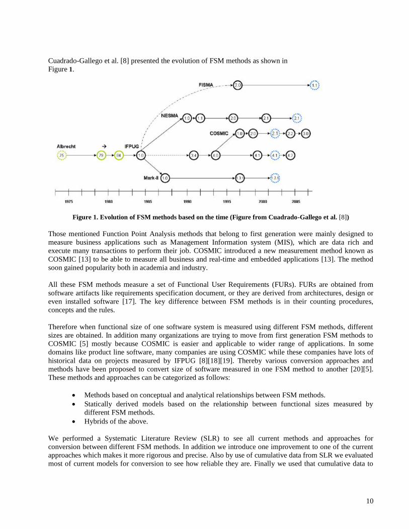
Cuadrado-Gallego et al. [8] presented the evolution of FSM methods as shown in
Figure 1.
Figure 1. Evolution of FSM methods based on the time (Figure from Cuadrado-Gallego et al. [8])
Those mentioned Function Point Analysis methods that belong to first generation were mainly designed to
measure business applications such as Management Information system (MIS), which are data rich and
execute many transactions to perform their job. COSMIC introduced a new measurement method known as
COSMIC [13] to be able to measure all business and real-time and embedded applications [13]. The method
soon gained popularity both in academia and industry.
All these FSM methods measure a set of Functional User Requirements (FURs). FURs are obtained from
software artifacts like requirements specification document, or they are derived from architectures, design or
even installed software [17]. The key difference between FSM methods is in their counting procedures,
concepts and the rules.
Therefore when functional size of one software system is measured using different FSM methods, different
sizes are obtained. In addition many organizations are trying to move from first generation FSM methods to
COSMIC [5] mostly because COSMIC is easier and applicable to wider range of applications. In some
domains like product line software, many companies are using COSMIC while these companies have lots of
historical data on projects measured by IFPUG [8][18][19]. Thereby various conversion approaches and
methods have been proposed to convert size of software measured in one FSM method to another [20][5].
These methods and approaches can be categorized as follows:
Methods based on conceptual and analytical relationships between FSM methods.
Statically derived models based on the relationship between functional sizes measured by
different FSM methods.
Hybrids of the above.
We performed a Systematic Literature Review (SLR) to see all current methods and approaches for
conversion between different FSM methods. In addition we introduce one improvement to one of the current
approaches which makes it more rigorous and precise. Also by use of cumulative data from SLR we evaluated
most of current models for conversion to see how reliable they are. Finally we used that cumulative data to
11
build a new model with more data points. This latter confirms finding of literature, but interestingly in another
way.
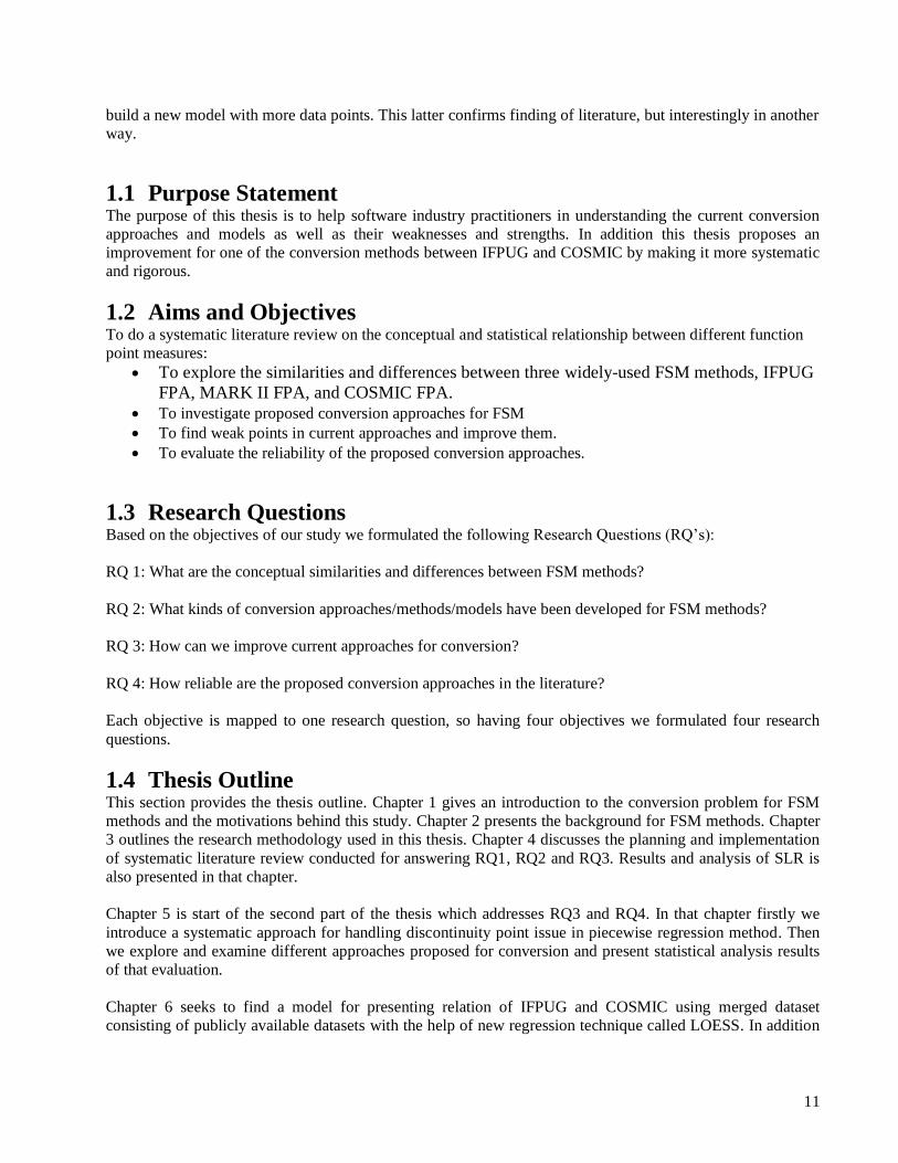
1.1 Purpose Statement The purpose of this thesis is to help software industry practitioners in understanding the current conversion
approaches and models as well as their weaknesses and strengths. In addition this thesis proposes an
improvement for one of the conversion methods between IFPUG and COSMIC by making it more systematic
and rigorous.
1.2 Aims and Objectives To do a systematic literature review on the conceptual and statistical relationship between different function
point measures:
To explore the similarities and differences between three widely-used FSM methods, IFPUG
FPA, MARK II FPA, and COSMIC FPA.
To investigate proposed conversion approaches for FSM
To find weak points in current approaches and improve them.
To evaluate the reliability of the proposed conversion approaches.
1.3 Research Questions Based on the objectives of our study we formulated the following Research Questions (RQ‘s):
RQ 1: What are the conceptual similarities and differences between FSM methods?
RQ 2: What kinds of conversion approaches/methods/models have been developed for FSM methods?
RQ 3: How can we improve current approaches for conversion?
RQ 4: How reliable are the proposed conversion approaches in the literature?
Each objective is mapped to one research question, so having four objectives we formulated four research
questions.
1.4 Thesis Outline This section provides the thesis outline. Chapter 1 gives an introduction to the conversion problem for FSM
methods and the motivations behind this study. Chapter 2 presents the background for FSM methods. Chapter
3 outlines the research methodology used in this thesis. Chapter 4 discusses the planning and implementation
of systematic literature review conducted for answering RQ1, RQ2 and RQ3. Results and analysis of SLR is
also presented in that chapter.
Chapter 5 is start of the second part of the thesis which addresses RQ3 and RQ4. In that chapter firstly we
introduce a systematic approach for handling discontinuity point issue in piecewise regression method. Then
we explore and examine different approaches proposed for conversion and present statistical analysis results
of that evaluation.
Chapter 6 seeks to find a model for presenting relation of IFPUG and COSMIC using merged dataset
consisting of publicly available datasets with the help of new regression technique called LOESS. In addition

12
we propose a new model derived from 134 data points. In making that model we used our systematic
approach.
Chapter 7 discusses major findings in answering research questions of our study. The threats to validity
during our study are presented in chapter 8. Finally chapter 9 ends up with conclusion of our study and
provides clues for the future work.
13
2 BACKGROUND In the following sections we discuss three widely-used Functional Size Measurement (FSM) methods; i.e.,
IFPUG FPA, COSMIC and Mark II FPA. It should be noted that for the sake of brevity, here we covered an
abstract view of each process without going into details. For more information readers can look at each
method‘s manual. Definition of terms used in whole thesis and in describing each method can be found in the
Glossary section at the end of this thesis.
2.1 ISO 14143 Standard on FSM International Standard Organization (ISO) and International Electrotechnical Commission (IEC) form the
specialized system for worldwide standardization. In 1994 ISO assembled working bodies for establishing
international standard for functional size measurement. They produced ISO/IEC 14143 series
[21][22][23][24][25][26] with a set of standards and technical documents of functional size measurement
methods. The six parts of ISO/IEC 14143 series are:
Part 1: ISO/IEC 14143-1 published in 1998, is about Definition of concepts; its scope is ―to define the
fundamental concepts of Functional Size Measurement (FSM) and describe the general principles for
applying an FSM method‖ [1].
Part 2: ISO/IEC 14143-2 published in 2002 deals with Conformity evaluation of software size measurement
methods to ISO; its aim is ―to establish a frame work and describes the process for the conformity evaluation
of a candidate FSM method against the provisions of ISO/IEC 14143-1:1998. It also provided guidelines for
determining the competence of conformity evaluation teams and a checklist to assist the conformity
evaluation of standard FSM method‖ [22].
Part 3: ISO/IEC 14143-3:2003 is about the Verification of functional size measurement methods; the scope of
this part is “to establish a framework for verifying the statements of an FSM method and/or for conducting
the tests requested by the verification sponsor” [23].
Part 4: ISO/IEC 14143-4:2002 defines a Reference model; its scope is ―to be used in verifying a FSM method‖
[24].
Part 5: ISO/IEC 14143-5:2004 is about Determination of functional domains for use with functional size
measurement; the scope of this part is “to describe the characteristics of functional domains and procedures
by which characteristics of Functional User Requirements (FUR) can be used to determine functional
domains” [25].
Part 6: ISO/IEC 14143-6:2005 is a Guide for use of ISO/IEC 14143 series and related International
Standards; ―it provides a summary of FSM related standards and relationships between them‖ [26]
The definitions of some major fundamental concepts of FSM method are given below:
Functional User Requirement (FUR):“A subset of user requirements, the FUR represents the user
practices and procedures that the software must perform to fulfill the users‟ needs. They exclude
quality requirements and any technical requirements” [21].
Base Functional Component (BFC):“Elementary unit of FUR defined by and used by a functional size measurement method for measurement purposes” [21].
14
Base Functional Component Type (BFC Types):“Defined Category of BFCs. A BFC is classified
as one and only one BFC type” [21].
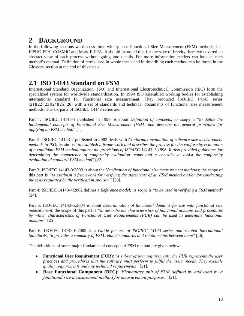
2.2 IFPUG FPA Albrecht‘s IFPUG FPA (ISO/IEC 20926:2003) was designed to measure business information systems [14]
[6]. The measurement procedure of IFPUG FPA is shown in Figure 2.
Figure 2. IFPUG FPA measurement process
An elementary process is, ―the smallest unit of activity that is meaningful to the user(s)‖ [14]. IFPUG FPA
Base Functional Component Types are:
1. Transactional Functions (TF): The three types of TF are:
1.1. External Input (EI): An EI is “an elementary process that processes data or control
information that comes from outside the application‟s boundary” [14].
1.2. External Output (EO): An EO is “an elementary process that sends data or control
information outside the application‟s boundary. The processing logic contains at least one
mathematical formula or calculation or creates derived data” [14].
1.3. External Inquiry (EQ): An EQ is “an elementary process that sends data or control
information outside the application boundary. The processing logic contains no mathematical
formula or calculation and creates no derived data” [14].
2. Data Functions: The two types of DF are:
1. Identify Elementary Processes from Functional User
Requirements
2. Identify Base Functional Components and their types
3. Rate the complexity of each BFC type
4. Assign function points to each BFC type according to the
complexity ratio
5. Calculate the function size by summing the FPs assigned
to each distinct BFC type
15
2.1. Internal Logical File (ILF): An ILF is “a user identifiable group of logically related data or
control information maintained within the boundary of application. The primary intent of ILF
is to hold data maintained through one or more elementary processes of the application
being counted” [14].
2.2. External Interface File (EIF): An EIF is “a user identifiable group of logically related data
or control information referenced by the application but maintained within the boundary of
another application. The primary intent of EIF is to hold data referenced through one or
more elementary processes within the boundary of the application counted” [14].
After identifying BFC types the complexities are rated. The process of assigning these complexities is as
follows:
Rate the Transaction Function: For the identified EI, EO and EQ one of low/average/high
complexity rating is assigned by counting number of Data Element Types (DETs) and File Types
Referenced (FTRs). These DETs and FTRs are counted according to the counting procedures for EI,
EO and EQ stated in IFPUG manual [14]. Complexity matrix of TFs is shown in Table 2.
Rate the Data Function: For the ILF and EIF one of low/average/high complexity rating is assigned
by counting number of Data Element Types (DETs) and Record Element Types (RETs). These are
also counted according to the counting procedures stated in IFPUG manual [14]. Complexity matrix
of TFs is shown in Table 3.
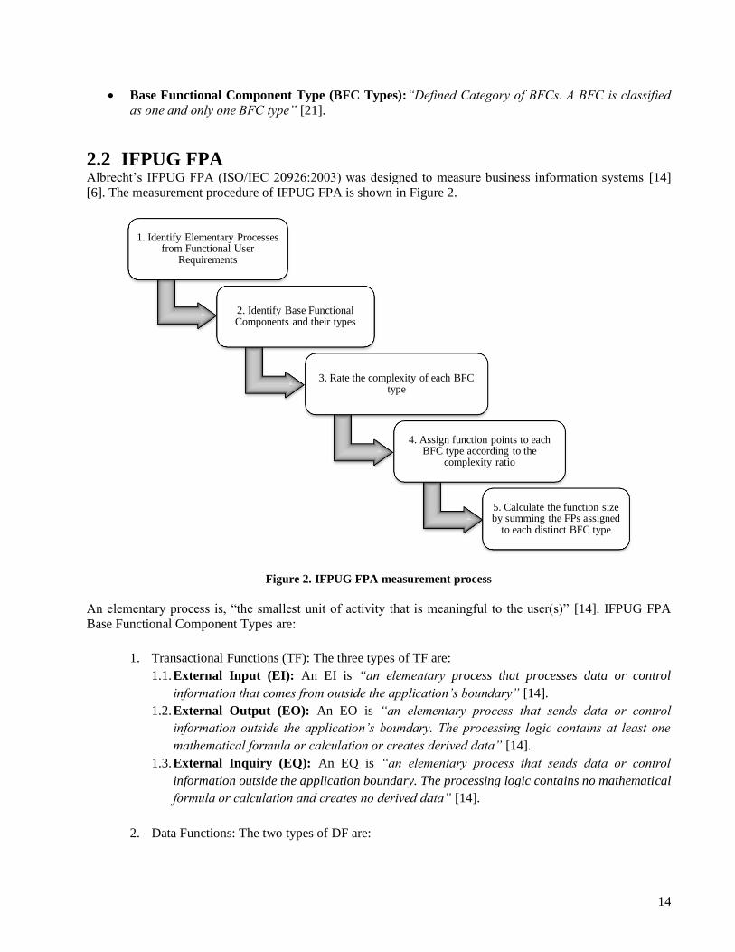
Table 2. Complexity matrix of EI, EO and EQ [14]
External Input 1 to 4 DET 5 to 15 DET 16 or more DET
0 to 1 FTR Low Low Average
2 FTRs Low Average High
3 or more FTRs Average High High
External
Output
&
External
Inquiries
1 to 5 DET 6 to 19 DET 20 or more DET
0 to 1 FTR Low Low Average
2 to 3 FTRs Low Average High
4 or more FTRs Average High High
Table 3. Complexity matrix of ILF and EIF [14]
Internal Logical
File & External
1 to 19 DET 20 to 50 DET 51 or more DET
1 RET Low Low Average

16
Interface File 2 to 5 RET Low Average High
6 or more RET Average High High
The IFPUG application user view is shown in Figure 3 (adopted from Galorath and Evans [27]):
Figure 3. Application user view in IFPUG FPA (originally from Galorath and Evans [27])
There is a table in manual that determines contribution of each BFC type according to its rated complexity
value (low/average/high). By summing all these numbers we obtain functional size of software system which
is called Unadjusted Function Point.
2.3 COSMIC COSMIC (ISO/IEC 19761:2003) [28] was developed to measure the functional size of business application
software, real time software and hybrid of these [29][30]. COSMIC measurement takes place in two phases:
COSMIC Mapping phase: Functional processes are identified from FURs of software artifact. A
functional process is “an elementary component of a set of Functional User Requirements comprising
a unique, cohesive and independently executable set of data movements” [13]. For each functional
process the data groups and respective data attributes are identified.
COSMIC Measurement phase: In this phase the data movements associated with each functional
process are identified and measurement function is applied. This step is repeated for all functional
process and finally aggregates the results with output of functional size in COSMIC CFP.
Prior to identifying of functional processes the following steps has to be done:
1. Identifying functional user: Functional user for business application may be humans and other peer
applications with which the application interfaces. Functional user for real time application may be
engineered hardware devices or other interfacing peer software.
2. Boundary: Functional users interact with the software being measured and the boundary lies
between the functional user and software.
Functional process is triggered by a data movement from the functional user and is complete when it has
executed all that has to be done in response to triggering event [28]. COSMIC manual provides certain rules
in identifying these functional processes. COSMIC measurement method is based on identifying and counting
data movements for each functional process which moves data group of an object of interest. A group of data
attributes forms a data group which are unique and distinguishable related to one object of interest in software
17
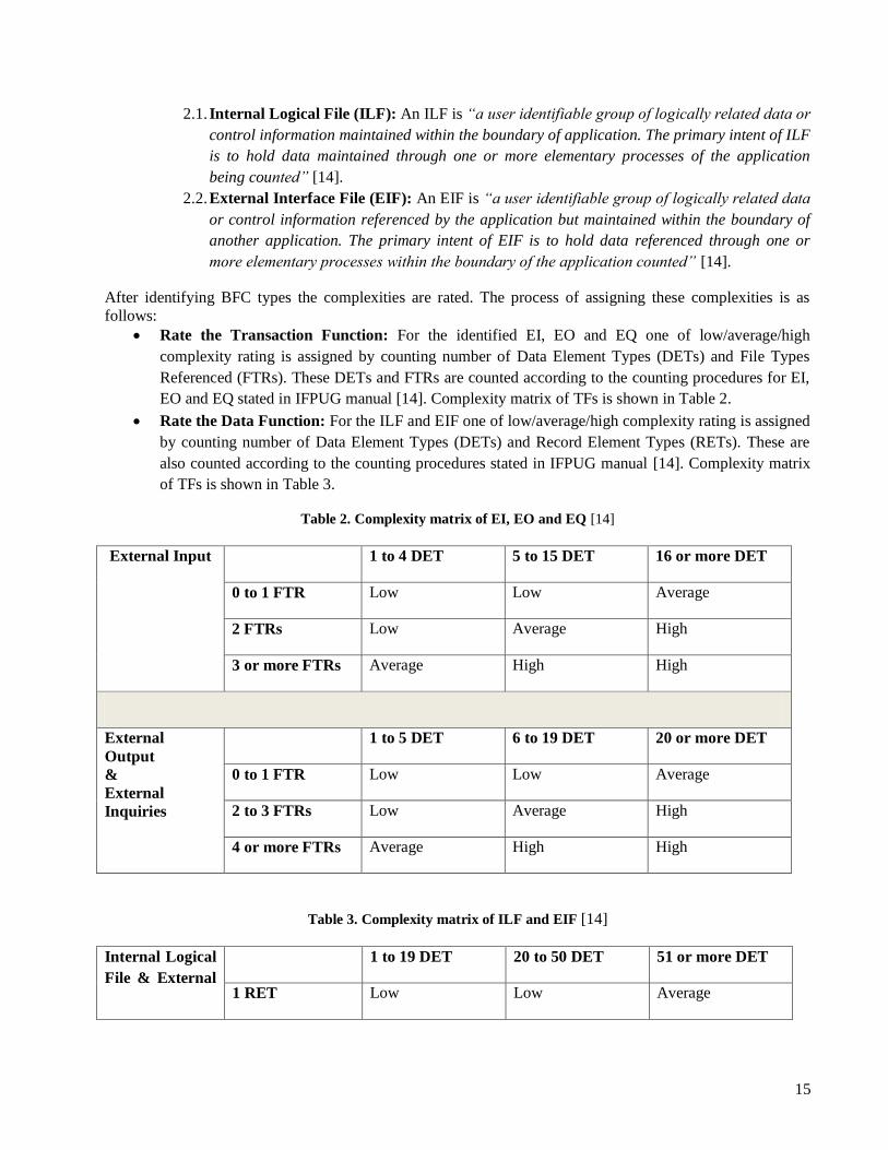
FURs. Figure 4 shows application view in COSMIC measurement process. The Data movements which move
data group are of four types:
i. Entry (E): ―A data movement that moves a data group from a functional user across the
boundary into the functional process where it is required‖ [13].
ii. Exit (X): ―A data movement that moves a data group from a functional process across the
boundary to the functional user that requires it” [13].
iii. Read (R): “A data movement that moves a data group from persistent storage within reach of the
functional process which requires it” [13].
iv. Write (W): “A data movement that moves a data group lying inside a functional process to
persistent storage”[13].
Figure 4. Application view in COSMIC measurement process
The size of software in COSMIC CFP is calculated as:
SizeCFP(functional processi) = ∑ (Entriesi) + ∑ (Exitsi) +∑ (Readsi) + ∑ (Writesi)
2.4 Mark II FPA Mark II (Mk II) FPA [31] was developed to measure business information systems. Mk II (ISO/IEC
20968:2002) [10] measures functional size independent of technology or methods used to develop or
implement software. It measures functional size of any software application that is described in terms of
logical transactions each comprising an input, process and an output component. Mk II method assists in
measuring process efficiency and managing costs for application software development, change or
maintenance activities [10]. The measurement process of Mk II FPA is as follows:
1. Identify Logical transactions (LT) from FURs where LT is “a smallest complete unit of information
processing that is meaningful to the end user in the business” [10]. 2. Identify and categorize Data Entity Types (DET).
3. For each LT:

18
3.1. Count number of input data element types (Ni) “which is proportional to number of uniquely
processed DETs composing the input side of transaction”[10]. 3.2. Data element types referenced (Ne) “which is proportional to number of uniquely processed
DETs or entities referenced during the course of logical transaction”[10]. 3.3. Number of output data element types (No) “which is proportional to number of uniquely
processed DETs composing the output side of transaction” [10].
4. Function Point Index (FPI) for application is:
FPI = Wi* ∑ i + We * ∑ e + Wo* ∑ o
Where Wi is weight per input data element type = 0.58
We is weight per data element type reference = 1.66
W0 is weight per output data element type = 0.26
19
3 RESEARCH METHODOLOGY Research is defined as ―Original investigation undertaken in order to gain knowledge and understanding‖
[32]. According to Brendtsson et al. [33] there are two types of research methods qualitative and quantitative.
In order to answer our research questions for this thesis, we designed our research methodology as described
in following paragraphs:
In order to answer RQ1 (What are the conceptual similarities and differences between FSM methods?) and
RQ2 (What kinds of conversion approaches/methods/models have been developed for FSM methods?) we
performed a Systematic Literature Review (SLR) followed by narrative and comparative analysis. Systematic
review provides us an opportunity of investigating primary studies on conversion methods and approaches as
well as similarities and differences between FSM methods. The results of SLR are summarized with help of
narrative analysis. Furthermore based on common grounds of concepts and by means of Comparative
Analysis, IFPUG, COSMIC and Mark II are compared.
To answer RQ3 (How can we improve current approaches for conversion?) we made analysis on the data
collected from SLR. Indeed answering RQ1 and RQ2 can provide us enough information to answer RQ3 as
well. Then we provided a suggestion for improving one of the conversion methods through a more systematic
and rigorous approach.
Finally to answer RQ4 (How reliable are the proposed conversion approaches in the literature?) we will use a
set of well-known and popular statistics to measure accuracy and predictive power of approach. In this part
we only deal with those models that are built using empirical data and are statistically-based conversion
formulas. Figure 5 shows a view of the research methodologies used to answer different questions.
3.1 Systematic Literature Review The main rationale for performing a systematic literature review is that in each research there is a need for
reviewing previous works in order to intensify the current knowledge and lay the foundations for new work to
stand on. But most of research kickoff with traditional literature review which is of little scientific value due
to non-rigorous and unfair approach [34]. According to Kitchenham [34] Systematic Literature Review (SLR)
is defined as ―A means of identifying, evaluating and interpreting all available research relevant to a
particular research question or topic area or phenomena of interest‖. SLR is also referred as systematic
reviews. Systematic reviews are a form of secondary studies which include individual studies called primary
studies [34]. Systematic reviews are undertaken for summarizing the existing evidences, identifying the gaps
in current research and providing a framework or background for new research activities [34].
Followings are the main features that distinguish systematic literature reviews:
Being started by a defined review protocol addressing specific research questions,
Defined search strategy in order to identify the relevant literature,
Explicit quality criteria for assessing quality of studies.
Being well documented such that the process can be repeated by other readers.
The SLR processes adopted by authors in this thesis are Kitchenham‘s ―Guidelines for performing systematic
literature review‖ [34] and Paula Mian et al.‘s ―A Systematic review process for software engineering‖ [35].
Due to lack of a detailed structure for review protocols suggested by Kitchenham we used protocols by Paula
Mian et al. for design of review protocols in our thesis. Because Mian et al.‘s guideline provides detailed
template for selection of keywords and question formulation while there are not much detail for these in
Kitchenhamn‘s guideline. So for the main SLR we used Kitchenhamn‘s guideline while just in review

20
protocols we used Mian et al.‘s guidelines. In addition we (authors of this thesis) used snowball sampling
[36][37] to avoid missing important studies not found during study selection of literature review.
Systematic review is conducted mainly in three phases [38]:
1. Planning the review: Need for SLR is identified and review protocol is developed.
2. Conducting the review: Selection of primary studies, quality assessment, data extraction and data
synthesis are done in this phase.
3. Reporting the review: SLR results are reported and the process is documented.
Systematic Literature ReviewSnowball Sampling
RQ1 RQ2 RQ3
Kitchenham Guidelines
Data Analysis and Synthesis
Narrative Analysis
Comparative Analysis
Statistical Analysis
Answer of RQ1
Answer of RQ2
Answer to RQ4
Answer of RQ3
Mian et al.’sGuidelines
Figure 5. Research methodology used to answer RQs.

21
3.1.1 Snowball Sampling Snowball sampling in social science is defined as ―a non-probabilistic form of sampling in which persons
initially chosen for the sample are used as informants to locate other persons having necessary
characteristics making them eligible for sample‖ [39]. In our thesis we used snowball sampling to explore
references of found literature. Among those references we want to see if any new article exists that our search
strings was unable to find. This was done to decrease any chance of missing related important works.
3.2 Data Analysis/Synthesis Data Analysis/synthesis is used for analyzing and evaluating the primary studies by selecting appropriate
methods for integrating [40] or providing new interpretative explanations from the studies [41]. For this SLR
we used the following techniques:
3.2.1 Narrative Analysis Narrative analysis can be used in both reviews of qualitative and quantitative research [42]. In the context of
systematic reviews narrative analysis is the most commonly used method for data analysis. According to
Rodgers et al. ―Narrative analysis is a defining characteristic of which is the adoption of narrative (as
opposed to statistical) summary of the findings of studies to the process of synthesis. This may occur
alongside or instead of statistical meta-analysis and does not exclude other numerical analyses‖ [43]. In
addition to describing our findings, it typically involves selection, chronicling and ordering of findings from
literature [44]. The results help us to perform interpretation on the higher levels of abstraction. According to
UK ERSC research methods programme, findings of narrative summary help us to identify the future work
needed in that area [45]. During this analysis phase, the results were tabulated and classified.
3.2.2 Comparative Analysis Comparative Analysis is used to contrast two things for identifying similarities and differences between the
entities [46]. The commonalities and diversities can be analyzed by constructing Boolean truth table [44]. For
an entity some portion of data or statement are identified and compared with remaining entities. To perform a
comparative analysis we can use different approaches like lens approach, frame of reference etc. [46]. We
used frame of reference which uses some umbrella concepts to make comparison between different entities. It
is suggested that the frame of reference be chosen from a source rather than being constructed by the authors
[46]. We used common concepts of FSM methods already mentioned in literature and manuals as frame of
reference and we put our discussion based on them.
3.2.3 Statistical Analysis Statistical analysis helps us to draw more reliable conclusions [47]. In our thesis for RQ4 for evaluation of
current approaches the results were analyzed statistically which are discussed in Analysis section. For
statistical analysis we used R [48] with its GUIs i.e. Red-R [49], and JGR [50]. Along them we used Deducer
[51] and Mintab [52] as additional statistical packages for analyzing the results.
3.2.4 Alternative Methods Possible alternatives of systematic literature review are traditional literature review, systematic mappings and
tertiary reviews. As we mentioned before traditional reviews lack the needed rigor, so systematic literature
reviews are preferred. Systematic mappings usually address broader areas compared to systematic literature
review [34]. In addition, analysis part of systematic mappings is less focused on the details of the topic [34].
So, again doing a systematic literature review preferred for addressing details of each study. Tertiary studies
come into play when you have different systematic literature reviews on the topic. In our case we couldn‘t
find any systematic literature review on this topic and our SLR is the first one.
In analysis part among the toolset of different qualitative and quantitative methods we used a handful of tools.
One of the other possible methods that we didn‘t use is Grounded Theory [53] [54]. Since grounded theory

22
has preconditions that didn‘t comply for our situation, we preferred to ignore that in our study. One major
condition in Grounded Theory is that you shouldn‘t have any pre-conceived ideas regarding data in your mind
[55]. We had done an exploratory study and we were familiar with categorization of different approaches for
conversion by studying articles and COSMIC manual [56]. So we felt that this judgment may influence our
categorization unconsciously.
Another popular option is meta-analysis [57] that is widely used in different disciplines. The focus of meta-
analysis is ―the impact of variable X on variable Y‖ [57]. That means researcher should review all the literature
he found to find evidences that how an independent variable affects outcome i.e. dependent variable. Since
our aim was not to study effect of any particular variable we were not able to employ meta-analysis on our
analysis and synthesis part. Our goal was to extract similarities and differences that exist among different
FSM methods regardless of how a special variable can cause those similarities and differences.
One another approach that can be used in our study is Thematic analysis [44]. Thematic analysis overlaps
with other methods like Narrative analysis and Content analysis [44]. Thematic analysis is more restrictive for
us compared to Narrative analysis since Thematic analysis tries to find recurring themes in the data [44]. This
latter property of Thematic analysis can be achieved by Narrative analysis as well. The difference is that
Narrative analysis is more flexible with not focusing just on finding special recurring theme in the data.
23
4 SYSTEMATIC LITERATURE REVIEW The literature review is done thoroughly to provide a result with high scientific value [38]. We have done an
exploratory literature review in the first phase of the research i.e. writing proposal. From the results of that
study we understood that all literature focus on conversion between IFPUG, COSMIC, and Mark II. In
addition the focus is mainly in conversion from IFPUG to COSMIC since most organizations try to shift from
first generation to second generation of FSM methods. Also there are some articles that discuss NESMA
method but this discussions are not more than just a few sentences. On the other hand FiSMA is not
mentioned in any article discussing conversion of FSM methods. Due to this fact for performing SLR we
didn‘t take into account FiSMA FSM. Based on well-known approaches for performing systematic literature
review in software engineering [38], we divided the review into distinct steps: specifying research questions,
developing and validating review protocol, searching relevant studies, assessing quality, and finally data
analysis and synthesis. The review process phases are illustrated as follows:
4.1 Planning
4.1.1 The Need for a Systematic Review Prior to conducting systematic review we searched IEEE, Inspec/Compendex, ISI, Scopus, and Science Direct
databases in order to identify whether any systematic review regarding Functional Size Measurement
Analysis exists or not. The string used for this search is:
({Function Point Analysis} OR FPA OR {functional size measurement} OR FSM OR {Function Point}) AND
({systematic review} OR {research review} OR {systematic literature review})
There were no results for this search. Hence we identified that there is a need to perform a systematic review.
4.1.2 Specifying Research Questions
We formulated four research questions that we think can address our concerns. First and second questions are
answered by SLR. In addition as mentioned before we use results of RQ1 and RQ2 to answer our third
research question. We perform SLR based on following two questions:
RQ1: what are the conceptual similarities and differences between FSM methods?
RQ2: what kind of conversion approaches/methods/models have been developed for FSM methods?
4.1.3 Defining Keywords We have used a modified version of the approach by Mian et al [35] for defining the details of each research
question. The results are as follows:
RQ1: SR protocol template: what are the conceptual similarities and differences between FSM methods?
Question Formulation:
1.1. Question focus: study of conceptual relations and differences between different function point
measures.
1.2. Question Quality and Amplitude:
-Problem: Type of conceptual similarities and differences between different FSM methods.
-Question: What are the conceptual similarities and differences between FSM methods?
24
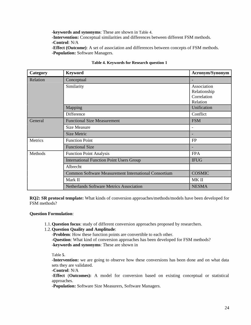
-keywords and synonyms: These are shown in Table 4.
-Intervention: Conceptual similarities and differences between different FSM methods.
-Control: N/A
-Effect (Outcome): A set of association and differences between concepts of FSM methods.
-Population: Software Managers.
Table 4. Keywords for Research question 1
Category Keyword Acronym/Synonym
Relation Conceptual -
Similarity Association
Relationship
Correlation
Relation
Mapping Unification
Difference Conflict
General Functional Size Measurement FSM
Size Measure -
Size Metric -
Metrics Function Point FP
Functional Size -
Methods Function Point Analysis FPA
International Function Point Users Group IFUG
Albrecht
Common Software Measurement International Consortium COSMIC
Mark II MK II
Netherlands Software Metrics Association NESMA
RQ2: SR protocol template: What kinds of conversion approaches/methods/models have been developed for
FSM methods?
Question Formulation:
1.1. Question focus: study of different conversion approaches proposed by researchers.
1.2. Question Quality and Amplitude:
-Problem: How these function points are convertible to each other.
-Question: What kind of conversion approaches has been developed for FSM methods?
-keywords and synonyms: These are shown in
Table 5. -Intervention: we are going to observe how these conversions has been done and on what data
sets they are validated.
-Control: N/A
-Effect (Outcomes): A model for conversion based on existing conceptual or statistical
approaches.
-Population: Software Size Measurers, Software Managers.
25
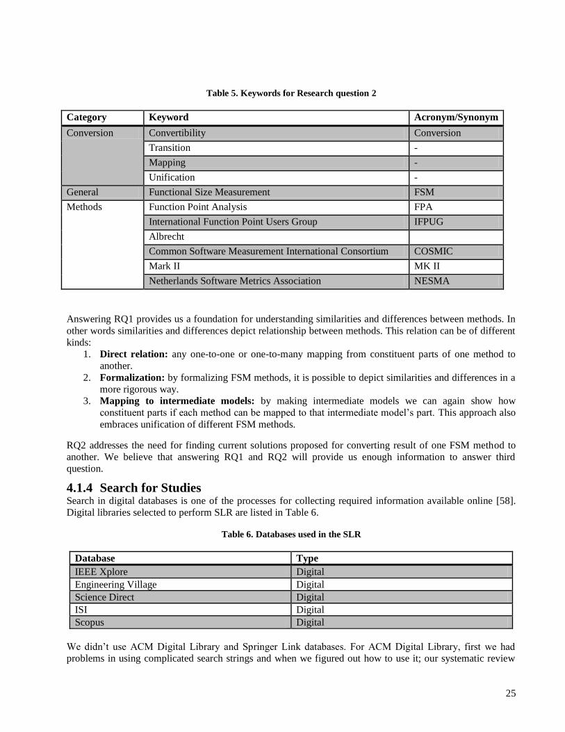
Table 5. Keywords for Research question 2
Category Keyword Acronym/Synonym
Conversion Convertibility Conversion
Transition -
Mapping -
Unification -
General Functional Size Measurement FSM
Methods Function Point Analysis FPA
International Function Point Users Group IFPUG
Albrecht
Common Software Measurement International Consortium COSMIC
Mark II MK II
Netherlands Software Metrics Association NESMA
Answering RQ1 provides us a foundation for understanding similarities and differences between methods. In
other words similarities and differences depict relationship between methods. This relation can be of different
kinds:
1. Direct relation: any one-to-one or one-to-many mapping from constituent parts of one method to
another.
2. Formalization: by formalizing FSM methods, it is possible to depict similarities and differences in a
more rigorous way.
3. Mapping to intermediate models: by making intermediate models we can again show how
constituent parts if each method can be mapped to that intermediate model‘s part. This approach also
embraces unification of different FSM methods.
RQ2 addresses the need for finding current solutions proposed for converting result of one FSM method to
another. We believe that answering RQ1 and RQ2 will provide us enough information to answer third
question.
4.1.4 Search for Studies Search in digital databases is one of the processes for collecting required information available online [58].
Digital libraries selected to perform SLR are listed in Table 6.
Table 6. Databases used in the SLR
Database Type
IEEE Xplore Digital
Engineering Village Digital
Science Direct Digital
ISI Digital
Scopus Digital
We didn‘t use ACM Digital Library and Springer Link databases. For ACM Digital Library, first we had
problems in using complicated search strings and when we figured out how to use it; our systematic review

26
was nearly done. For not using Springer Link the reason was inability of this database to handle complex
search strings.
4.1.5 Study Selection Criteria Selection criteria are different based on each research question. For the first question we have:
-Exclusion criteria:
Studies not related to software engineering
Studies not related to function points
Studies which are not peer reviewed
Studies in languages other than English
-Inclusion criteria:
Studies covering similarities and differences between at least two of mentioned FSM methods
Studies that try to formalize one or more techniques which this formalization can help to understand
conceptual association between techniques
Studies that try to map techniques to an intermediate model e.g. UML or try to come with a unified
model consisting of common features of methods
Second question has the same rules for excluding articles as the first question, but here inclusion criterion is
as follows:
Studies discussing function point conversion between IFPUG, NESMA, COSMIC and Mk II.
4.1.6 Study Selection Procedure This phase is done by both authors (two persons) separately and to see degree of agreement between the two.
Kappa coefficient [59] is applied which we will cover in upcoming sections. Databases were explored and
primary studies were selected based on inclusion/exclusion criteria.
4.1.7 Study Quality Assessment Selected primary studies were assessed against quality assessment checklist with a simple scale with values of
‗Yes‘ or ‗No‘ [60]. We prepared quality assessment checklist based on guidelines from [38] as shown in
Table 7. If a study fulfills assessment criteria then it is filled with value ‗Yes‘ else with ‗No‘.
Table 7. Quality Assessment Checklist
No. Quality Assessment Criteria Yes/No
1 Are the aims clearly stated?
2 Are the data collection methods adequately described?
3 Are the research methods used clearly described?
4 Are the validity threats (limitations, constraints etc.) discussed?
5 Are the citations properly referred?
Based on results of simple scale values associated with assessment of study, studies are grouped under three
categories of high quality, average quality and low quality. If a particular study has quality assessment with 4
or more ‗yes‘ then it is considered as study with high quality. A study which satisfies criteria of having three
‗yes‘, is grouped under average quality and studies with 2 or less ‗yes‘ are grouped into low quality.
27
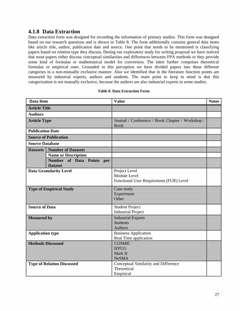
4.1.8 Data Extraction Data extraction form was designed for recording the information of primary studies. This form was designed
based on our research questions and is shown in Table 8. The form additionally contains general data items
like article title, author, publication date and source. One point that needs to be mentioned is classifying
papers based on relation type they discuss. During our exploratory study for writing proposal we have noticed
that most papers either discuss conceptual similarities and differences between FPA methods or they provide
some kind of formulas or mathematical model for conversion. The latter further comprises theoretical
formulas or empirical ones. Grounded in this perception we have divided papers into these different
categories in a non-mutually exclusive manner. Also we identified that in the literature function points are
measured by industrial experts, authors and students. The main point to keep in mind is that this
categorization is not mutually exclusive, because the authors are also industrial experts in some studies.
Table 8. Data Extraction Form
Data Item Value Notes
Article Title
Authors
Article Type Journal / Conference / Book Chapter / Workshop /
Book
Publication Date
Source of Publication
Source Database
Datasets Number of Datasets
Name or Description
Number of Data Points per
Dataset
Data Granularity Level Project Level
Module Level
Functional User Requirement (FUR) Level
Type of Empirical Study Case study
Experiment
Other
Source of Data Student Project
Industrial Project
Measured by Industrial Experts
Students
Authors
Application type Business Application
Real Time application
Methods Discussed COSMIC
IFPUG
Mark II
NeSMA
Type of Relation Discussed Conceptual Similarity and Difference
Theoretical
Empirical

28
4.1.9 Data Analysis and Synthesis Data synthesis is used to summarize the collected data, by combining small different pieces into a single unit
by using qualitative or quantitative synthesis [38]. For the findings of our systematic review we used narrative
analysis [43] to list similarities and differences between the methods. We also categorized and tabulated the
results of conversion models.
4.1.10 Pilot Study Pilot study is necessary for a good research strategy and is used to identify the deficiencies of the research
design procedure. In systematic review a pilot study aims to assure a mutual agreement on review process
between the two authors before conducting the review [38]. Primarily three papers were taken and authors
read them individually and completed data extraction form. Then they discussed differences in their findings
by comparing the forms. After that authors updated the forms based on their findings during pilot study.
4.2 Conducting the Review
4.2.1 Identification of Research The primary studies are identified in SLR by forming a search strategy related to the research questions [38].
In this search strategy strings are formulated based on trial search on combination of keywords and
synonyms. In our thesis, as discussed in review protocol in Section 4.1.3 search stings were formulated for
research questions RQ1 and RQ2 by combining keywords listed in Table 4 and
Table 5 respectively. Our supervisor validated search strings during formulation and after finalizing them. The
search strings are listed in Table 9.
Table 9. Search Strings for systematic review
RQ1 (( Conceptual OR Similarity OR Association OR Relation OR Relationship OR Correlation OR
Mapping OR Unification OR Difference OR Conflict ) AND ( ("Functional Size Measurement" OR
FSM) OR "Size Measure" OR "Size Metric" ) OR (( "Function Point" OR FP ) OR "Functional Size"
) OR ( ("Function Point Analysis" OR FPA) OR ("International Function Point Users Group" OR
IFPUG) OR Albrecht OR ( "Common Software Measurement International Consortium" OR
COSMIC ) OR ( "Mark II" OR "MK II") OR ("Netherlands Software Metrics Association" OR
NESMA)))
RQ2 ("International Function point Users Group" OR IFPUG OR "Function Point Analysis" OR FPA OR
Albrecht OR "functional size measurement" OR FSM OR "common software measurement
International consortium" OR COSMIC OR "Netherlands software metrics association" OR NESMA
OR "Mark II" OR Mk II) AND (conver* OR transition OR mapping OR unification)
4.2.2 Articles Selection Criteria To select most relevant articles, we followed a procedure which is shown in Figure 6. After obtaining initial
list of papers from databases we applied database specific refinement on that list. By database specific
refinement we mean refinement by the subject or classification codes that vary between different databases.
For instance, IEEE Xplore has the facility to limit the searches to Computing subject while Engineering
Village provides exclusion and inclusion of articles based on classification codes. The next step was to
observe articles‘ title to determine if they are relevant or not. For the first question each article discussing
relationship between different FSM methods was chosen as a candidate article. For second question applying
inclusion criteria only makes selection possible for articles that discuss conversion. If any doubt exist that an
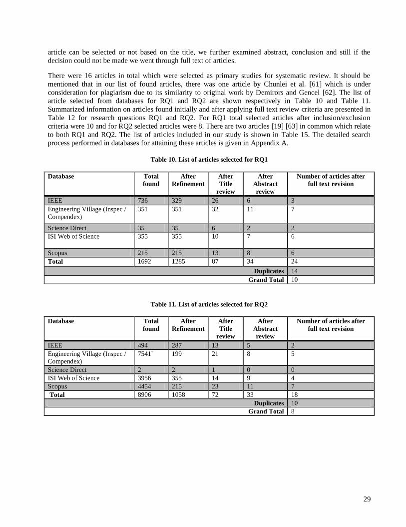
29
article can be selected or not based on the title, we further examined abstract, conclusion and still if the
decision could not be made we went through full text of articles.
There were 16 articles in total which were selected as primary studies for systematic review. It should be
mentioned that in our list of found articles, there was one article by Chunlei et al. [61] which is under
consideration for plagiarism due to its similarity to original work by Demirors and Gencel [62]. The list of
article selected from databases for RQ1 and RQ2 are shown respectively in Table 10 and Table 11.
Summarized information on articles found initially and after applying full text review criteria are presented in
Table 12 for research questions RQ1 and RQ2. For RQ1 total selected articles after inclusion/exclusion
criteria were 10 and for RQ2 selected articles were 8. There are two articles [19] [63] in common which relate
to both RQ1 and RQ2. The list of articles included in our study is shown in Table 15. The detailed search
process performed in databases for attaining these articles is given in Appendix A.
Table 10. List of articles selected for RQ1
Database Total
found
After
Refinement
After
Title
review
After
Abstract
review
Number of articles after
full text revision
IEEE 736 329 26 6 3
Engineering Village (Inspec /
Compendex)
351 351 32 11 7
Science Direct 35 35 6 2 2
ISI Web of Science 355 355 10 7 6
Scopus 215 215 13 8 6
Total 1692 1285 87 34 24
Duplicates 14
Grand Total 10
Table 11. List of articles selected for RQ2
Database Total
found
After
Refinement
After
Title
review
After
Abstract
review
Number of articles after
full text revision
IEEE 494 287 13 5 2
Engineering Village (Inspec /
Compendex)
7541` 199 21 8 5
Science Direct 2 2 1 0 0
ISI Web of Science 3956 355 14 9 4
Scopus 4454 215 23 11 7
Total 8906 1058 72 33 18
Duplicates 10
Grand Total 8
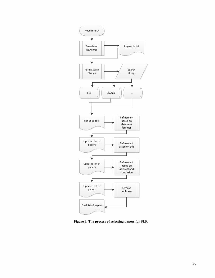
30
Need for SLR
Search for keywords
Keywords list
Form Search Strings
Search Strings
IEEE Scopus ...
List of papersRefinement
based on databasefacilities
Updated list of papers
Refinement based on title
Updated list of papers
Refinement based on
abstract and conclusion
Updated list of papers
Remove duplicates
Final list of papers
Figure 6. The process of selecting papers for SLR
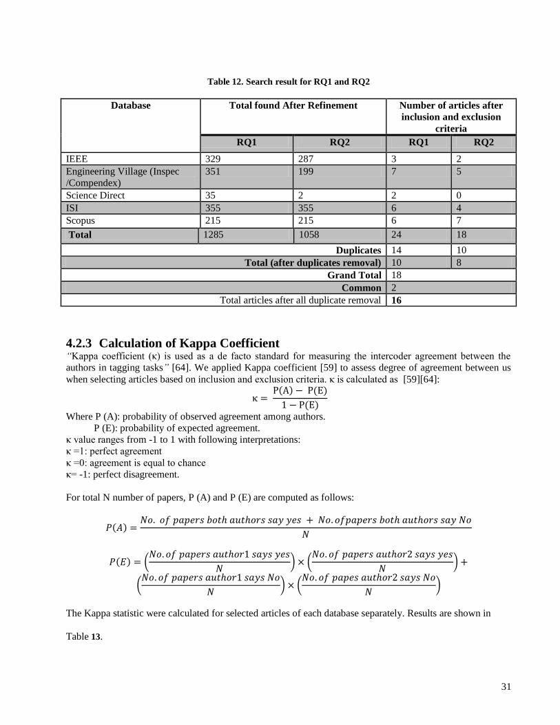
31
Table 12. Search result for RQ1 and RQ2
Database Total found After Refinement
Number of articles after
inclusion and exclusion
criteria
RQ1 RQ2 RQ1 RQ2
IEEE 329 287 3 2
Engineering Village (Inspec
/Compendex)
351 199 7 5
Science Direct 35 2 2 0
ISI 355 355 6 4
Scopus 215 215 6 7
Total 1285 1058 24 18
Duplicates 14 10
Total (after duplicates removal) 10 8
Grand Total 18
Common 2
Total articles after all duplicate removal 16
4.2.3 Calculation of Kappa Coefficient “Kappa coefficient (κ) is used as a de facto standard for measuring the intercoder agreement between the
authors in tagging tasks” [64]. We applied Kappa coefficient [59] to assess degree of agreement between us
when selecting articles based on inclusion and exclusion criteria. κ is calculated as [59][64]:
( ) ( )
( )
Where P (A): probability of observed agreement among authors.
P (E): probability of expected agreement.
κ value ranges from -1 to 1 with following interpretations:
κ =1: perfect agreement
κ =0: agreement is equal to chance
κ= -1: perfect disagreement.
For total N number of papers, P (A) and P (E) are computed as follows:
( )
( ) (
) (
)
(
) (
)
The Kappa statistic were calculated for selected articles of each database separately. Results are shown in
Table 13.

32
Table 13. Calculated Kappa coefficient for each database
Database Name Calculated Kappa Value
IEEE 0.67
Engineering Village 0.95
Science Direct 1
ISI 0.89
Scopus 0.82
Average 0.86
The kappa value of IEEE database is low due to the disagreement between the authors in including three
studies [65][66][67]. These articles were irrelevant to the study according to perspective of one author and
after a clear discussion and reviewing the full text these are excluded. There were also some disagreements in
inclusion of papers [19], [63] in results of RQ1 or RQ2. Since there were some common aspects which
mentioned papers discuss both conceptual similarities and differences and also theoretical formula, we
decided to include these studies in both questions‘ result.
4.2.4 Snowball Sampling Snowball sampling is an iterative study of articles selecting from references of one article. We used snowball
sampling in our thesis for building a good scope and in order to prevent missing other studies related to our
topic. First, references of 16 articles from our primary study were explored and we identified 10 new articles.
In Second step these 10 newly found articles‘ references were explored and no more studies related to our
topic were identified. The selection of studies using snowball sampling is based on defined
inclusion/exclusion criteria as in Section 4.1.5. The process of snowball sampling performed for set of articles
is shown in Figure 7. In that figure, ‗IS‘ stands for Initial Set of articles that we had, and ‗FS‘ stands for Final
Set of articles that we have after snowball sampling. Four articles [68] [18] [16] [20] were retrieved from
―Google Scholar‖, other four [69] [70] [71] [15] from authors‘ website and two articles [62] [72] are provided
by our supervisor Dr. Cigdem Gencel. We also searched previously mentioned digital databases for titles of
our snowball sampling papers and there were no search result. This search made us sure that there is no
problem in our selection of keywords for string formulation. Since missed articles by our search strings were
not available in databases.
4.2.5 Selected Articles for Study Total number of identified primary studies for conducting our systematic review was 26 articles (16 from
database search + 10 snowball sampling) as shown in Table 14. The final list of articles included in our study
from both database search and snowball sampling is shown in Table 15.
Table 14. Articles selected from databases and snowball sampling
Search Articles References
Database 16 [31][73][1][74][75][19][76][77][63][17][5][78][79][8][80][81]
Snowball sampling 10 [69][70][71][68][18][16][20][72][1][62]
Total 26
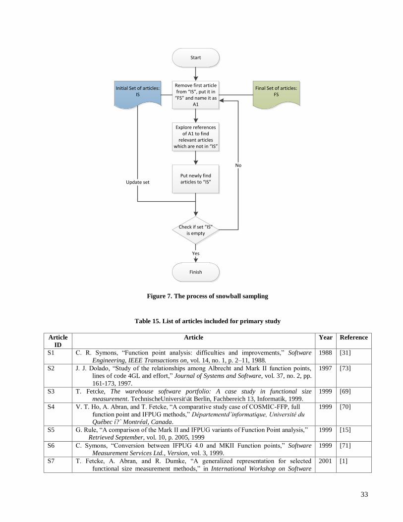
33
Start
Initial Set of articles: IS
Explore references of A1 to find
relevant articles which are not in “IS”
Put newly find articles to “IS”
Check if set “IS” is empty
Remove first article from “IS”, put it in
“FS” and name it as A1
Update set
No
Finish
Yes
Final Set of articles: FS
Figure 7. The process of snowball sampling
Table 15. List of articles included for primary study
Article
ID
Article Year Reference
S1 C. R. Symons, ―Function point analysis: difficulties and improvements,‖ Software
Engineering, IEEE Transactions on, vol. 14, no. 1, p. 2–11, 1988.
1988 [31]
S2 J. J. Dolado, ―Study of the relationships among Albrecht and Mark II function points,
lines of code 4GL and effort,‖ Journal of Systems and Software, vol. 37, no. 2, pp.
161-173, 1997.
1997 [73]
S3 T. Fetcke, The warehouse software portfolio: A case study in functional size
measurement. TechnischeUniversit\ät Berlin, Fachbereich 13, Informatik, 1999.
1999 [69]
S4 V. T. Ho, A. Abran, and T. Fetcke, ―A comparative study case of COSMIC-FFP, full
function point and IFPUG methods,‖ Départementd‟informatique, Université du
Québec í?` Montréal, Canada.
1999 [70]
S5 G. Rule, ―A comparison of the Mark II and IFPUG variants of Function Point analysis,‖
Retrieved September, vol. 10, p. 2005, 1999
1999 [15]
S6 C. Symons, ―Conversion between IFPUG 4.0 and MKII Function points,‖ Software
Measurement Services Ltd., Version, vol. 3, 1999.
1999 [71]
S7 T. Fetcke, A. Abran, and R. Dumke, ―A generalized representation for selected
functional size measurement methods,‖ in International Workshop on Software
2001 [1]
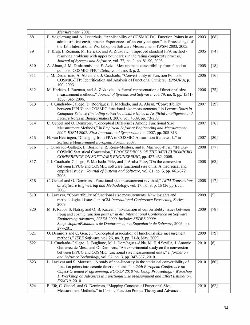
34
Measurement, 2001.
S8 F. Vogelezang and A. Lesterhuis, ―Applicability of COSMIC Full Function Points in an
administrative environment: Experiences of an early adopter,‖ in Proceedings of
the 13th International Workshop on Software Measurement–IWSM 2003, 2003.
2003 [68]
S9 T. Kralj, I. Rozman, M. Hericko, and A. Zivkovic, ―Improved standard FPA method -
resolving problems with upper boundaries in the rating complexity process,‖
Journal of Systems and Software, vol. 77, no. 2, pp. 81-90, 2005.
2005 [74]
S10 A. Abran, J. M. Desharnais, and F. Aziz, ―Measurement convertibility-from function
points to COSMIC-FFP,‖ Delta, vol. 4, no. 3, p. 2.
2005 [18]
S11 J. M. Desharnais, A. Abran, and J. Cuadrado, ―Convertibility of Function Points to
COSMIC-FFP: Identification and Analysis of Functional Outliers,‖ ENSUR A, p.
190, 2006.
2006 [16]
S12 M. Hericko, I. Rozman, and A. Zivkovic, ―A formal representation of functional size
measurement methods,‖ Journal of Systems and Software, vol. 79, no. 9, pp. 1341-
1358, Sep. 2006.
2006 [75]
S13 J. J. Cuadrado-Gallego, D. Rodríguez, F. Machado, and A. Abran, ―Convertibility
between IFPUG and COSMIC functional size measurements,‖ in Lecture Notes in
Computer Science (including subseries Lecture Notes in Artificial Intelligence and
Lecture Notes in Bioinformatics), 2007, vol. 4589, pp. 73-283.
2007 [19]
S14 C. Gencel and O. Demirors, ―Conceptual Differences Among Functional Size
Measurement Methods,‖ in Empirical Software Engineering and Measurement,
2007. ESEM 2007. First International Symposium on, 2007, pp. 305-313.
2007 [76]
S15 H. van Heeringen, ―Changing from FPA to COSMIC-A transition framework,‖ in
Software Measurement European Forum, 2007.
2007 [20]
S16 J. Cuadrado-Gallego, L. Buglione, R. Rejas-Muslera, and F. Machado-Piriz, ―IFPUG-
COSMIC Statistical Conversion,‖ PROCEEDINGS OF THE 34TH EUROMICRO
CONFERENCE ON SOFTWARE ENGINEERING, pp. 427-432, 2008.
2008 [77]
S17 J. J. Cuadrado-Gallego, F. Machado-Piriz, and J. Aroba-Paez, ―On the conversion
between IFPUG and COSMIC software functional size units: A theoretical and
empirical study,‖ Journal of Systems and Software, vol. 81, no. 5, pp. 661-672,
2008.
2008 [63]
S18 C. Gencel and O. Demirors, ―Functional size measurement revisited,‖ ACM Transactions
on Software Engineering and Methodology, vol. 17, no. 3, p. 15 (36 pp.), Jun.
2008.
2008 [17]
S19 L. Lavazza, ―Convertibility of functional size measurements: New insights and
methodological issues,‖ in ACM International Conference Proceeding Series,
2009.
2009 [5]
S20 M. F. Rabbi, S. Natraj, and O. B. Kazeem, ―Evaluation of convertibility issues between
ifpug and cosmic function points,‖ in 4th International Conference on Software
Engineering Advances, ICSEA 2009, Includes SEDES 2009:
SimposioparaEstudantes de DoutoramentoemEngenharia de Software, 2009, pp.
277-281.
2009 [78]
S21 O. Demirors and C. Gencel, ―Conceptual association of functional size measurement
methods,‖ IEEE Software, vol. 26, no. 3, pp. 71-8, May. 2009.
2009 [79]
S22 J. J. Cuadrado-Gallego, L. Buglione, M. J. Domínguez-Alda, M. F. d Sevilla, J. Antonio
Gutierrez de Mesa, and O. Demirors, ―An experimental study on the conversion
between IFPUG and COSMIC functional size measurement units,‖ Information
and Software Technology, vol. 52, no. 3, pp. 347-357, 2010.
2010 [8]
S23 L. Lavazza and S. Morasca, ―A study of non-linearity in the statistical convertibility of
function points into cosmic function points,‖ in 24th European Conference on
Object-Oriented Programming, ECOOP 2010 Workshop Proceedings - Workshop
1: Workshop on Advances in Functional Size Measurement and Effort Estimation,
FSM‟10, 2010.
2010 [80]
S24 P. Efe, C. Gencel, and O. Demirors, ―Mapping Concepts of Functional Size
Measurement Methods,‖ in Cosmic Function Points: Theory and Advanced
2010 [62]
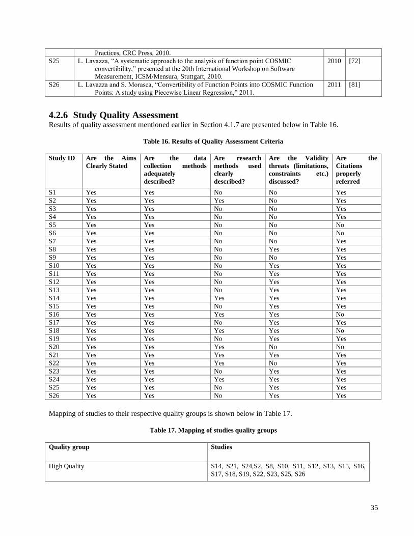
35
Practices, CRC Press, 2010.
S25 L. Lavazza, ―A systematic approach to the analysis of function point COSMIC
convertibility,‖ presented at the 20th International Workshop on Software
Measurement, ICSM/Mensura, Stuttgart, 2010.
2010 [72]
S26 L. Lavazza and S. Morasca, ―Convertibility of Function Points into COSMIC Function
Points: A study using Piecewise Linear Regression,‖ 2011.
2011 [81]
4.2.6 Study Quality Assessment Results of quality assessment mentioned earlier in Section 4.1.7 are presented below in Table 16.
Table 16. Results of Quality Assessment Criteria
Study ID Are the Aims
Clearly Stated
Are the data
collection methods
adequately
described?
Are research
methods used
clearly
described?
Are the Validity
threats (limitations,
constraints etc.)
discussed?
Are the
Citations
properly
referred
S1 Yes Yes No No Yes
S2 Yes Yes Yes No Yes
S3 Yes Yes No No Yes
S4 Yes Yes No No Yes
S5 Yes Yes No No No
S6 Yes Yes No No No
S7 Yes Yes No No Yes
S8 Yes Yes No Yes Yes
S9 Yes Yes No No Yes
S10 Yes Yes No Yes Yes
S11 Yes Yes No Yes Yes
S12 Yes Yes No Yes Yes
S13 Yes Yes No Yes Yes
S14 Yes Yes Yes Yes Yes
S15 Yes Yes No Yes Yes
S16 Yes Yes Yes Yes No
S17 Yes Yes No Yes Yes
S18 Yes Yes Yes Yes No
S19 Yes Yes No Yes Yes
S20 Yes Yes Yes No No
S21 Yes Yes Yes Yes Yes
S22 Yes Yes Yes No Yes
S23 Yes Yes No Yes Yes
S24 Yes Yes Yes Yes Yes
S25 Yes Yes No Yes Yes
S26 Yes Yes No Yes Yes
Mapping of studies to their respective quality groups is shown below in Table 17.
Table 17. Mapping of studies quality groups
Quality group Studies
High Quality S14, S21, S24,S2, S8, S10, S11, S12, S13, S15, S16,
S17, S18, S19, S22, S23, S25, S26
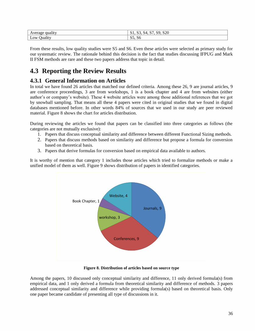
36
Average quality S1, S3, S4, S7, S9, S20
Low Quality S5, S6
From these results, low quality studies were S5 and S6. Even these articles were selected as primary study for
our systematic review. The rationale behind this decision is the fact that studies discussing IFPUG and Mark
II FSM methods are rare and these two papers address that topic in detail.
4.3 Reporting the Review Results
4.3.1 General Information on Articles In total we have found 26 articles that matched our defined criteria. Among these 26, 9 are journal articles, 9
are conference proceedings, 3 are from workshops, 1 is a book chapter and 4 are from websites (either
author‘s or company‘s website). These 4 website articles were among those additional references that we got
by snowball sampling. That means all these 4 papers were cited in original studies that we found in digital
databases mentioned before. In other words 84% of sources that we used in our study are peer reviewed
material. Figure 8 shows the chart for articles distribution.
During reviewing the articles we found that papers can be classified into three categories as follows (the
categories are not mutually exclusive):
1. Papers that discuss conceptual similarity and difference between different Functional Sizing methods.
2. Papers that discuss methods based on similarity and difference but propose a formula for conversion
based on theoretical basis. 3. Papers that derive formulas for conversion based on empirical data available to authors.
It is worthy of mention that category 1 includes those articles which tried to formalize methods or make a
unified model of them as well. Figure 9 shows distribution of papers in identified categories.
Figure 8. Distribution of articles based on source type
Among the papers, 10 discussed only conceptual similarity and difference, 11 only derived formula(s) from
empirical data, and 1 only derived a formula from theoretical similarity and difference of methods. 3 papers
addressed conceptual similarity and difference while providing formula(s) based on theoretical basis. Only
one paper became candidate of presenting all type of discussions in it.
Journals, 9
Conferences, 9
workshop, 3
Book Chapter, 1
Website, 4

37
Figure 9. Distribution of articles based on identified categories
4.3.2 Data Extraction Results Next results are FPA methods covered in the article and type of relation that is discussed. Table 18 depicts
these results.
Table 18. Articles, methods discussed in each and type of relation that they discuss
Article Methods
Discussed
Type of
Relation
Note
IFP
UG
Mark
II
NeS
MA
CO
SM
IC
Con
ceptu
al
Em
pirica
l
Th
eoretica
l
Symons [31]
Dolado [73] No formula is proposed, only the correlation
Fetcke [69]
Ho et al [70]
Rule [15]
Symons [71]
Fetcke et al [1]
Vogelezang&Lesterhuis[68] NeSMA to COSMIC and IFPUG to COSMIC
Kralj et al [74]
Abran & Desharnais [18]
Desharnais et al [16]
Hericko et al [75]
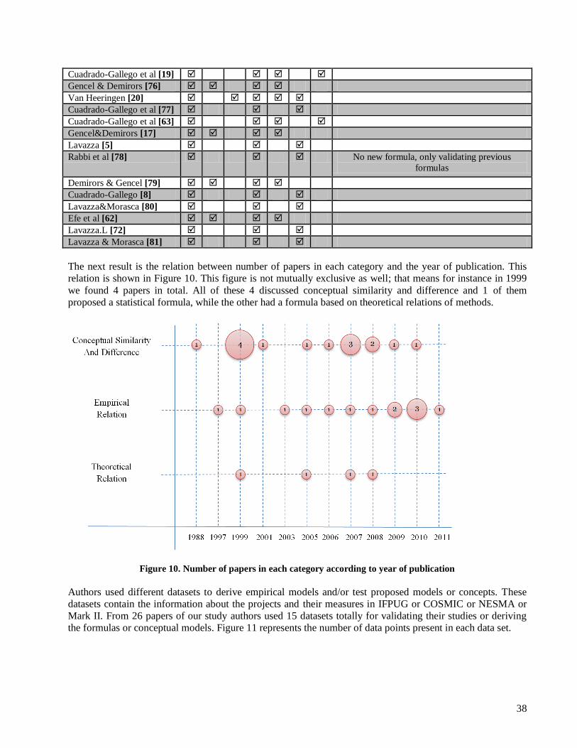
38
Cuadrado-Gallego et al [19]
Gencel & Demirors [76]
Van Heeringen [20]
Cuadrado-Gallego et al [77]
Cuadrado-Gallego et al [63]
Gencel&Demirors [17]
Lavazza [5]
Rabbi et al [78] No new formula, only validating previous
formulas
Demirors & Gencel [79]
Cuadrado-Gallego [8]
Lavazza&Morasca [80]
Efe et al [62]
Lavazza.L [72]
Lavazza & Morasca [81]
The next result is the relation between number of papers in each category and the year of publication. This
relation is shown in Figure 10. This figure is not mutually exclusive as well; that means for instance in 1999
we found 4 papers in total. All of these 4 discussed conceptual similarity and difference and 1 of them
proposed a statistical formula, while the other had a formula based on theoretical relations of methods.
Figure 10. Number of papers in each category according to year of publication
Authors used different datasets to derive empirical models and/or test proposed models or concepts. These
datasets contain the information about the projects and their measures in IFPUG or COSMIC or NESMA or
Mark II. From 26 papers of our study authors used 15 datasets totally for validating their studies or deriving
the formulas or conceptual models. Figure 11 represents the number of data points present in each data set.

39
Figure 11. Number of data points per data set
Among these 15 datasets mostly the data points contain industrial project data. Only two datasets i.e.
Cuadrdo-Gallego et al. 2007 and Dolado 1997 contain 30 and 24 academic projects respectively. Two
datasets, Cuadrado-Gallaego et al. 2008 (jjcg06) and Cuadrado-Gallaego et al. 2008 (jjcg07) contain real
world application, but measured by students under the guidance of junior researchers. Cuadrado-Gallaego et
al. 2010 (jjcg0607) is a combined dataset of Cuadrado-Gallaego et al. 2008 (jjcg06) and Cuadrado-Gallaego
et al. 2008 (jjcg07). The details of all these datasets are given in Appendix B.
4.4 Data Analysis & Results
4.4.1 Conceptual Similarities and Differences In this section we present results of systematic review. We divided this section into several subsections. Each
subsection seeks a goal that is related to other sections as well. First we provide a summary of all articles that
were found related to conceptual similarities and differences and how they contribute to the knowledge.
In the next section (Basis for Discussion) we presented those frames of references that we used for
comparison between different methods. Indeed this frame of reference is an abstract view of all FSM
methods. Right after that section we go to see what are similarities and differences in general. Next step is to
explore similarities and differences in basic definitions in each FSM method. FSM methods define some
common and some unique concepts which we explore in that part. Next we try to seek similarity and
difference in constituent parts which are building blocks of each method. We continue by presenting a
discussion on previously mentioned similarities and differences. In the final step we discuss roots and sources
of difference between FSM methods. Throughout this section we used the words ―similarity‖ and ―common‖
interchangeably.
First we try to define a frame of reference for laying the ground for fundamental concepts, and then we
discuss the similarities and differences that we found in the literature. In this study the focus is on IFPUG,
Mark II and COSMIC FSM methods.
24
30
5
39
11
6
14
3
1
26
21
14
35
1
1
2
Dolado 1997 (Academic projects)
Fetcke 1999 (warehouse portfolio)
Symons 1999 (Tony Hassan of KPMG Management…
Vogelezang & Lesterhuis al 2003 (Rabobank)
Abran et al 2005 (Desharnais 2005 dataset)
Desharnais et al 2006 (Desharnais 2006 Dataset)
Cuadrado-Gallaego et al 2007
Gencel & Demirors al 2007 (Military Inventory management)
Van Heeringen 2007 (Sogeti data set 2006)
Cuadrado-Gallaego et al 2008 (jjcg06)
Cuadrado-Gallaego et al 2008 (jjcg07)
Cuadrado-Gallaego et al 2010 (jjcg0607)
Rabbi et al 2009 (simple locator)
Rabbi et al 2009 (PCGeek)
Gencel & Demirors 2009 (Avionics management system)
Number of data points per dataset
Academic Projects Industry Projects
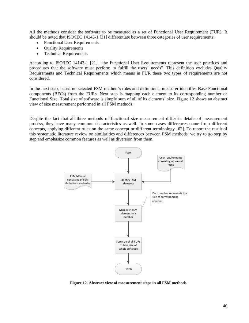
40
All the methods consider the software to be measured as a set of Functional User Requirement (FUR). It
should be noted that ISO/IEC 14143-1 [21] differentiate between three categories of user requirements:
Functional User Requirements
Quality Requirements
Technical Requirements
According to ISO/IEC 14143-1 [21], ―the Functional User Requirements represent the user practices and
procedures that the software must perform to fulfill the users‘ needs‖. This definition excludes Quality
Requirements and Technical Requirements which means in FUR these two types of requirements are not
considered.
In the next step, based on selected FSM method‘s rules and definitions, measurer identifies Base Functional
components (BFCs) from the FURs. Next step is mapping each element to its corresponding number or
Functional Size. Total size of software is simply sum of all of its elements‘ size. Figure 12 shows an abstract
view of size measurement performed in all FSM methods.
Despite the fact that all three methods of functional size measurement differ in details of measurement
process, they have many common characteristics as well. In some cases differences come from different
concepts, applying different rules on the same concept or different terminology [62]. To report the result of
this systematic literature review on similarities and differences between FSM methods, we try to go step by
step and emphasize common features as well as diversion from them.
Start
Identify FSM elements
User requirements consisting of several
FURs
FSM Manual consisting of FSM
definitions and rules
Map each FSM element to a
number
Sum size of all FURs to take size of
whole software
Finish
Each number represents the size of corresponding
element
Figure 12. Abstract view of measurement steps in all FSM methods
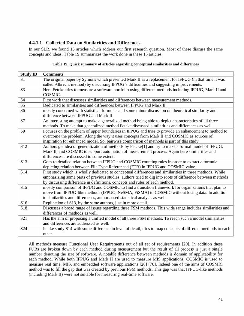
41
4.4.1.1 Collected Data on Similarities and Differences
In our SLR, we found 15 articles which address our first research question. Most of these discuss the same
concepts and ideas. Table 19 summarizes the work done in these 15 articles.
Table 19. Quick summary of articles regarding conceptual similarities and differences
Study ID Comments
S1 The original paper by Symons which presented Mark II as a replacement for IFPUG (in that time it was
called Albrecht method) by discussing IFPUG‘s difficulties and suggesting improvements.
S3 Here Fetcke tries to measure a software portfolio using different methods including IFPUG, Mark II and
COSMIC.
S4 First work that discusses similarities and differences between measurement methods.
S5 Dedicated to similarities and differences between IFPUG and Mark II.
S6 mostly concerned with statistical formulas and some minor discussion on theoretical similarity and
difference between IFPUG and Mark II
S7 An interesting attempt to make a generalized method being able to depict characteristics of all three
methods. To make that generalized method Fetcke discussed similarities and differences as well.
S9 Focuses on the problem of upper boundaries in IFPUG and tries to provide an enhancement to method to
overcome the problem. Along the way it uses concepts from Mark II and COSMIC as sources of
inspiration for enhanced model. So, pairwise comparison of methods is part of this study.
S12 Authors get idea of generalization of methods by Fetcke[1] and try to make a formal model of IFPUG,
Mark II, and COSMIC to support automation of measurement process. Again here similarities and
differences are discussed to some extent.
S13 Goes to detailed relation between IFPUG and COSMIC counting rules in order to extract a formula
depicting relation between File Type Referenced (FTR) in IFPUG and COSMIC value.
S14 First study which is wholly dedicated to conceptual differences and similarities in three methods. While
emphasizing some parts of previous studies, authors tried to dig into roots of difference between methods
by discussing difference in definitions, concepts and rules of each method.
S15 mostly comparison of IFPUG and COSMIC to find a transition framework for organizations that plan to
move from IFPUG-like methods (IFPUG, NeSMA, FiSMA) to COSMIC without losing data. In addition
to similarities and differences, authors used statistical analysis as well.
S16 Replication of S13, by the same authors, just in more detail.
S18 Discusses a broad range of issues regarding three FSM methods. This wide range includes similarities and
differences of methods as well.
S21 Has the aim of proposing a unified model of all three FSM methods. To reach such a model similarities
and differences are addressed as well.
S24 Is like study S14 with some difference in level of detail, tries to map concepts of different methods to each
other.
All methods measure Functional User Requirements out of all set of requirements [20]. In addition these
FURs are broken down by each method during measurement but the result of all process is just a single
number denoting the size of software. A notable difference between methods is domain of applicability for
each method. While both IFPUG and Mark II are used to measure MIS applications, COSMIC is used to
measure real time, MIS, and embedded software applications [28] [70]. Indeed one of the aims of COSMIC
method was to fill the gap that was created by previous FSM methods. This gap was that IFPUG-like methods
(including Mark II) were not suitable for measuring real-time software.
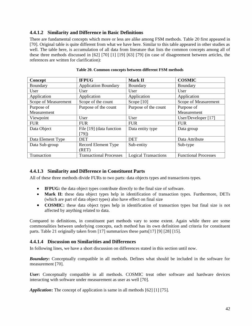
42
4.4.1.2 Similarity and Difference in Basic Definitions
There are fundamental concepts which more or less are alike among FSM methods. Table 20 first appeared in
[70]. Original table is quite different from what we have here. Similar to this table appeared in other studies as
well. The table here, is accumulation of all data from literature that lists the common concepts among all of
these three methods discussed in [62] [70] [1] [19] [63] [79] (in case of disagreement between articles, the
references are written for clarification):
Table 20. Common concepts between different FSM methods
Concept IFPUG Mark II COSMIC
Boundary Application Boundary Boundary Boundary
User User User User
Application Application Application Application
Scope of Measurement Scope of the count Scope [10] Scope of Measurement
Purpose of
Measurement
Purpose of the count Purpose of the count Purpose of
Measurement
Viewpoint User User User/Developer [17]
FUR FUR FUR FUR
Data Object File [19] (data function
[79])
Data entity type Data group
Data Element Type DET DET Data Attribute
Data Sub-group Record Element Type
(RET)
Sub-entity Sub-type
Transaction Transactional Processes Logical Transactions Functional Processes
4.4.1.3 Similarity and Difference in Constituent Parts
All of these three methods divide FURs to two parts: data objects types and transactions types.
IFPUG: the data object types contribute directly to the final size of software.
Mark II: these data object types help in identification of transaction types. Furthermore, DETs
(which are part of data object types) also have effect on final size
COSMIC: these data object types help in identification of transaction types but final size is not
affected by anything related to data.
Compared to definitions, in constituent part methods vary to some extent. Again while there are some
commonalities between underlying concepts, each method has its own definition and criteria for constituent
parts. Table 21 originally taken from [17] summarizes these parts[17] [9] [28] [15].
4.4.1.4 Discussion on Similarities and Differences
In following lines, we have a short discussion on differences stated in this section until now.
Boundary: Conceptually compatible in all methods. Defines what should be included in the software for
measurement [70].
User: Conceptually compatible in all methods. COSMIC treat other software and hardware devices
interacting with software under measurement as user as well [70].
Application: The concept of application is same in all methods [62] [1] [75].
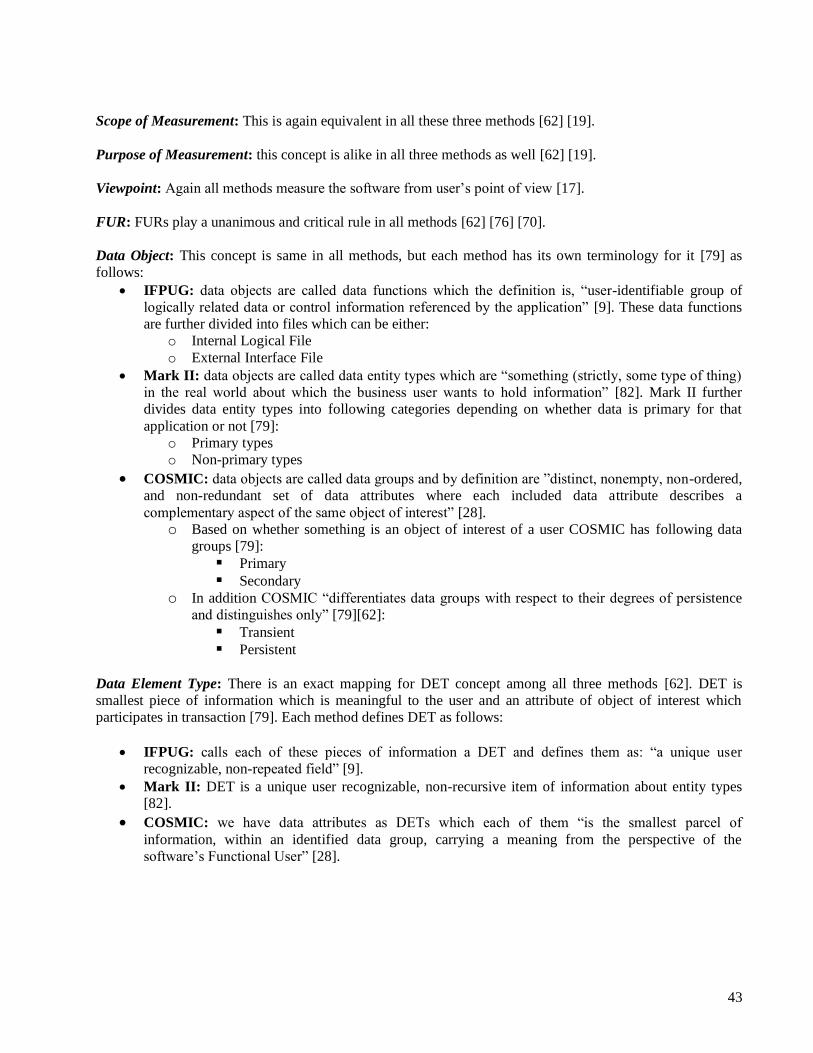
43
Scope of Measurement: This is again equivalent in all these three methods [62] [19].
Purpose of Measurement: this concept is alike in all three methods as well [62] [19].
Viewpoint: Again all methods measure the software from user‘s point of view [17].
FUR: FURs play a unanimous and critical rule in all methods [62] [76] [70].
Data Object: This concept is same in all methods, but each method has its own terminology for it [79] as
follows:
IFPUG: data objects are called data functions which the definition is, ―user-identifiable group of
logically related data or control information referenced by the application‖ [9]. These data functions
are further divided into files which can be either:
o Internal Logical File
o External Interface File
Mark II: data objects are called data entity types which are ―something (strictly, some type of thing)
in the real world about which the business user wants to hold information‖ [82]. Mark II further
divides data entity types into following categories depending on whether data is primary for that
application or not [79]:
o Primary types
o Non-primary types
COSMIC: data objects are called data groups and by definition are ‖distinct, nonempty, non-ordered,
and non-redundant set of data attributes where each included data attribute describes a
complementary aspect of the same object of interest‖ [28]. o Based on whether something is an object of interest of a user COSMIC has following data
groups [79]: Primary Secondary
o In addition COSMIC ―differentiates data groups with respect to their degrees of persistence
and distinguishes only‖ [79][62]: Transient Persistent
Data Element Type: There is an exact mapping for DET concept among all three methods [62]. DET is
smallest piece of information which is meaningful to the user and an attribute of object of interest which
participates in transaction [79]. Each method defines DET as follows:
IFPUG: calls each of these pieces of information a DET and defines them as: ―a unique user
recognizable, non-repeated field‖ [9].
Mark II: DET is a unique user recognizable, non-recursive item of information about entity types
[82].
COSMIC: we have data attributes as DETs which each of them ―is the smallest parcel of
information, within an identified data group, carrying a meaning from the perspective of the
software‘s Functional User‖ [28].

44
Table 21. Comparison of constituent parts of IFPUG, Mark II and COSMIC FSM methods (originally appeared in [17])
FSM
Method
BFC BFC Types BFC Constituent Parts BFC Attributes Counted Complexity
Weight
Contribution
to Size
IFPUG Elementary
Process
Transactional
Functions
EI Input/Output Message: cross
the boundary; input message to
persistent storage
DETs and File Type
Referenced (FTRs)
Small 3
Medium 4
Large 6
EO Input/Output Message: cross
the boundary; Output Message
from persistent storage with
derived data
DETs and FTRs Small 4
Medium 5
Large 7
EQ Input/Output Message: cross
the boundary; Output Message
from persistent storage with no
derived data
DETs and FTRs Small 3
Medium 4
Large 6
Data
Functions
ILF Persistent data group
maintained by the application
DETs and Record
Element Types (RETs)
Small 7
Medium 10
Large 15
EIF Persistent data group
maintained by another
application
DETs and RETs Small 5
Medium 7
Large 10
Mark II Logical
Transaction
Logical Transactions Input Message: must cross the
boundary, incoming
Data Element Types
(DETs)
- 0.58
Output Message: must cross
the boundary, outgoing
DETs - 0.26
Processing part: must be
wholly retained within the
boundary
References to the
Retained data expressed
logically as Entity Types
in third normal form
- 1.66
COSMIC Data
Movement
Type within a
Functional
Process
Entry Input Message: cross the
boundary, incoming
Entries - 1
Exit Output Message: cross the
boundary, outgoing
Exits - 1
Read Output Message: from
persistent storage, within the
boundary
Reads - 1
Write Input Message: to persistent
Storage, within the boundary
Writes - 1
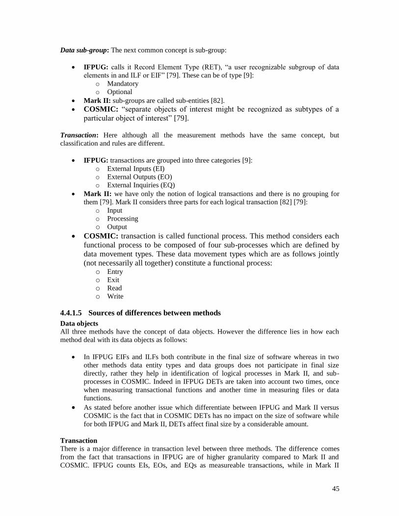
45
Data sub-group: The next common concept is sub-group:
IFPUG: calls it Record Element Type (RET), ―a user recognizable subgroup of data
elements in and ILF or EIF‖ [79]. These can be of type [9]:
o Mandatory
o Optional
Mark II: sub-groups are called sub-entities [82].
COSMIC: ―separate objects of interest might be recognized as subtypes of a
particular object of interest‖ [79].
Transaction: Here although all the measurement methods have the same concept, but
classification and rules are different.
IFPUG: transactions are grouped into three categories [9]:
o External Inputs (EI)
o External Outputs (EO)
o External Inquiries (EQ)
Mark II: we have only the notion of logical transactions and there is no grouping for
them [79]. Mark II considers three parts for each logical transaction [82] [79]:
o Input
o Processing
o Output
COSMIC: transaction is called functional process. This method considers each
functional process to be composed of four sub-processes which are defined by
data movement types. These data movement types which are as follows jointly
(not necessarily all together) constitute a functional process: o Entry o Exit o Read o Write
4.4.1.5 Sources of differences between methods
Data objects
All three methods have the concept of data objects. However the difference lies in how each
method deal with its data objects as follows:
In IFPUG EIFs and ILFs both contribute in the final size of software whereas in two
other methods data entity types and data groups does not participate in final size
directly, rather they help in identification of logical processes in Mark II, and sub-
processes in COSMIC. Indeed in IFPUG DETs are taken into account two times, once
when measuring transactional functions and another time in measuring files or data
functions.
As stated before another issue which differentiate between IFPUG and Mark II versus
COSMIC is the fact that in COSMIC DETs has no impact on the size of software while
for both IFPUG and Mark II, DETs affect final size by a considerable amount.
Transaction
There is a major difference in transaction level between three methods. The difference comes
from the fact that transactions in IFPUG are of higher granularity compared to Mark II and
COSMIC. IFPUG counts EIs, EOs, and EQs as measureable transactions, while in Mark II
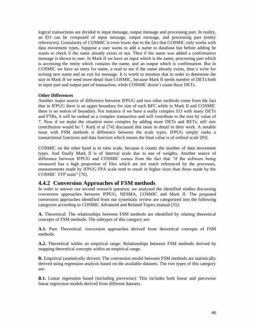
46
logical transactions are divided to input message, output message and processing part. In reality,
an EO can be composed of input message, output message, and processing part (entity
references). Granularity of COSMIC is even lower due to the fact that COSMIC only works with
data movement types. Suppose a user wants to add a name to database but before adding he
wants to check if the name already exists or not. Then if the name was added a confirmation
message is shown to user. In Mark II we have an input which is the name, processing part which
is accessing the entity which contains the name, and an output which is confirmation. But in
COSMIC we have an entry for name, a read to see if the name already exists, then a write for
writing new name and an exit for message. It is worth to mention that in order to determine the
size in Mark II we need more detail than COSMIC, because Mark II needs number of DETs both
in input part and output part of transaction, while COSMIC doesn‘t count these DETs.
Other Differences
Another major source of difference between IFPUG and two other methods come from the fact
that in IFPUG there is an upper boundary for size of each BFC while in Mark II and COSMIC
there is no notion of boundary. For instance if we have a really complex EO with many DETs
and FTRs, it will be ranked as a complex transaction and will contribute to the size by value of
7. Now if we make the situation more complex by adding more DETs and RETs, still size
contribution would be 7. Karlj et al [74] discussed this issue in detail in their work. A notable
issue with FSM methods is difference between the scale types. IFPUG simply ranks a
transactional functions and data function which means the final value is of ordinal scale [83].
COSMIC on the other hand is in ratio scale, because it counts the number of data movement
types. And finally Mark II is of Interval scale due to use of weights. Another source of
difference between IFPUG and COSMIC comes from the fact that ―if the software being
measured has a high proportion of files which are not much referenced by the processes,
measurements made by IFPUG FPA scale tend to result in higher sizes than those made by the
COSMIC FFP scale‖ [76].
4.4.2 Conversion Approaches of FSM methods In order to answer our second research question, we analyzed the identified studies discussing
conversion approaches between IFPUG, NESMA, COSMIC and Mark II. The proposed
conversion approaches identified from our systematic review are categorized into the following
categories according to COSMIC Advanced and Related Topics manual [55]:
A. Theoretical: The relationships between FSM methods are identified by relating theoretical
concepts of FSM methods. The subtypes of this category are:
A.1. Pure Theoretical: conversion approaches derived from theoretical concepts of FSM
methods.
A.2. Theoretical within an empirical range: Relationships between FSM methods derived by
mapping theoretical concepts within an empirical range.
B. Empirical (statistically driven): The conversion model between FSM methods are statistically
derived using regression analysis based on the available datasets. The two types of this category
are:
B.1. Linear regression based (including piecewise): This includes both linear and piecewise
linear regression models derived from different datasets.
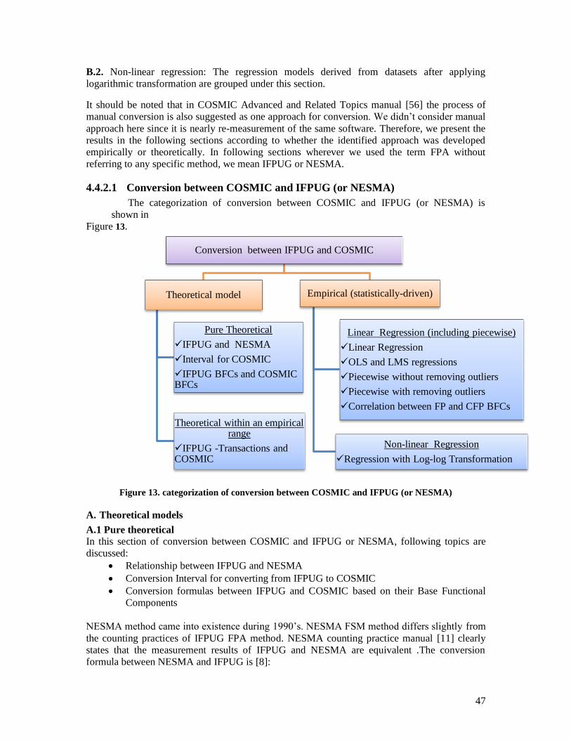
47
B.2. Non-linear regression: The regression models derived from datasets after applying
logarithmic transformation are grouped under this section.
It should be noted that in COSMIC Advanced and Related Topics manual [56] the process of
manual conversion is also suggested as one approach for conversion. We didn‘t consider manual
approach here since it is nearly re-measurement of the same software. Therefore, we present the
results in the following sections according to whether the identified approach was developed
empirically or theoretically. In following sections wherever we used the term FPA without
referring to any specific method, we mean IFPUG or NESMA.
4.4.2.1 Conversion between COSMIC and IFPUG (or NESMA)
The categorization of conversion between COSMIC and IFPUG (or NESMA) is
shown in
Figure 13.
Figure 13. categorization of conversion between COSMIC and IFPUG (or NESMA)
A. Theoretical models
A.1 Pure theoretical
In this section of conversion between COSMIC and IFPUG or NESMA, following topics are
discussed:
Relationship between IFPUG and NESMA
Conversion Interval for converting from IFPUG to COSMIC
Conversion formulas between IFPUG and COSMIC based on their Base Functional
Components
NESMA method came into existence during 1990‘s. NESMA FSM method differs slightly from
the counting practices of IFPUG FPA method. NESMA counting practice manual [11] clearly
states that the measurement results of IFPUG and NESMA are equivalent .The conversion
formula between NESMA and IFPUG is [8]:
Conversion between IFPUG and COSMIC
Theoretical model
Pure Theoretical
IFPUG and NESMA
Interval for COSMIC
IFPUG BFCs and COSMIC BFCs
Theoretical within an empirical range
IFPUG -Transactions and COSMIC
Empirical (statistically-driven)
Linear Regression (including piecewise)
Linear Regression
OLS and LMS regressions
Piecewise without removing outliers
Piecewise with removing outliers
Correlation between FP and CFP BFCs
Non-linear Regression
Regression with Log-log Transformation
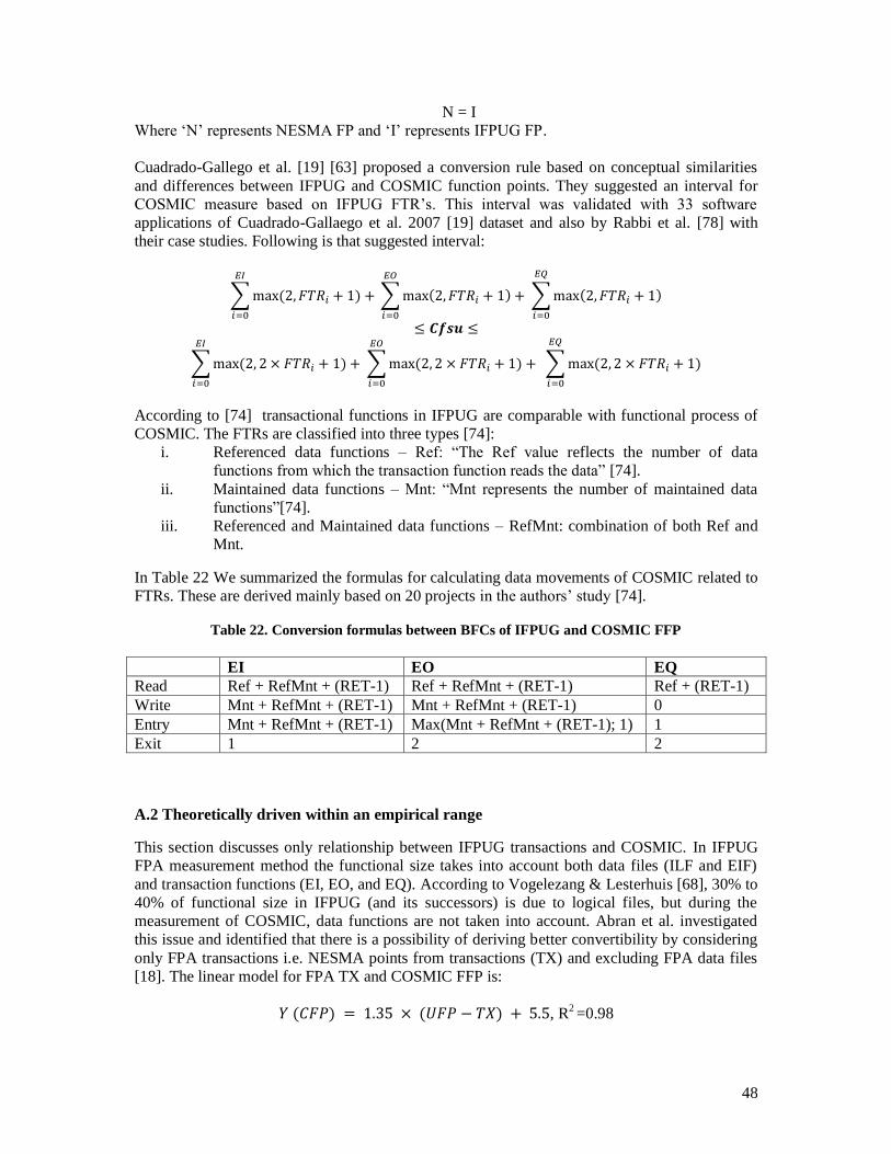
48
N = I
Where ‗N‘ represents NESMA FP and ‗I‘ represents IFPUG FP.
Cuadrado-Gallego et al. [19] [63] proposed a conversion rule based on conceptual similarities
and differences between IFPUG and COSMIC function points. They suggested an interval for
COSMIC measure based on IFPUG FTR‘s. This interval was validated with 33 software
applications of Cuadrado-Gallaego et al. 2007 [19] dataset and also by Rabbi et al. [78] with
their case studies. Following is that suggested interval:
∑ ( )
∑ ( ) ∑ ( )
∑ ( ) ∑ ( ) ∑ ( )
According to [74] transactional functions in IFPUG are comparable with functional process of
COSMIC. The FTRs are classified into three types [74]:
i. Referenced data functions – Ref: ―The Ref value reflects the number of data
functions from which the transaction function reads the data‖ [74].
ii. Maintained data functions – Mnt: ―Mnt represents the number of maintained data
functions‖[74].
iii. Referenced and Maintained data functions – RefMnt: combination of both Ref and
Mnt.
In Table 22 We summarized the formulas for calculating data movements of COSMIC related to
FTRs. These are derived mainly based on 20 projects in the authors‘ study [74].
Table 22. Conversion formulas between BFCs of IFPUG and COSMIC FFP
EI EO EQ
Read Ref + RefMnt + (RET-1) Ref + RefMnt + (RET-1) Ref + (RET-1)
Write Mnt + RefMnt + (RET-1) Mnt + RefMnt + (RET-1) 0
Entry Mnt + RefMnt + (RET-1) Max(Mnt + RefMnt + (RET-1); 1) 1
Exit 1 2 2
A.2 Theoretically driven within an empirical range
This section discusses only relationship between IFPUG transactions and COSMIC. In IFPUG
FPA measurement method the functional size takes into account both data files (ILF and EIF)
and transaction functions (EI, EO, and EQ). According to Vogelezang & Lesterhuis [68], 30% to
40% of functional size in IFPUG (and its successors) is due to logical files, but during the
measurement of COSMIC, data functions are not taken into account. Abran et al. investigated
this issue and identified that there is a possibility of deriving better convertibility by considering
only FPA transactions i.e. NESMA points from transactions (TX) and excluding FPA data files
[18]. The linear model for FPA TX and COSMIC FFP is:
( ) ( ) , R2 =0.98

49
R2 shows goodness of fit and the closer its value to 1 the better the model fits its data (more
detail on this comes in next section (section B.1 Linear Regression). There is a little
improvement in value of R2
(0.98) of FPA-TX and COSMIC compared to the result of R2
(0.91)
of FPA and COSMIC. The convertibility results for converging to absolute COSMIC size also
are improved [18].
Desharnais et al. [16] also presented a conversion model based on FPA transaction sizes and
COSMIC.
( ) ( ) , R2 = 0.98
Here also R2
value is better than the value derived based on FPA size 0.93 [16]. Other
improvements observed are [16]:
9 projects out of 14 have very small relative difference (difference between actual and
estimated) i.e. less than 5%
4 projects have a relative difference between 10% and 15%
1 project has relative difference of 35%.
Table 23 summarizes the results of linear models obtained based on FPA-TX and COSMIC.
Table 23. Linear models for FPA-TX and COSMIC FFP
Authors Dataset Conversion Formula R2
Abran et al. [18] Abran et al. 2005
(Desharnais 2005
dataset) [18]
( ) ( )
0.98
Desharnais et al.[16] Desharnais et al. 2006
(Desharnais 2006
Dataset) [16]
( ) ( )
0.98
B. Statistically-driven models
B.1 Linear Regression (incl. piecewise)
In this section following models for conversion between IFPUG and COSMIC are discussed:
Linear regression
OLS and LMS regressions
Piecewise linear without removing outliers
Piecewise linear with removing outliers
Correlation between FP and CFP BFCs
The relevant studies published about the conversion of functional size measurements shows that
there is a high correlation between IFPUG measurement and COSMIC functional size
measurement since both of these FSM methods quantify the same attribute of project i.e.
functional size. Many researchers used linear regression to establish a formula for conversion
between IFPUG and COSMIC. The resulting linear equations are in the form of:
Where C is the dependent variable i.e. COSMIC CFP, I is independent variable i.e. IFPUG FP, a
and b are parameters of straight line i.e. intercept and slope respectively. In all formulas based
on linear regression we have a statistic called coefficient of determination denoted by R2. ―It can
vary between 0 and 1 and measures the fit of regression equation‖ [84].

50
In following works, authors proposed relation between IFPUG and COSMIC and linear
regression is used to identify it. Datasets used by the authors for their studies are given in
Appendix B.
Vogelezang & Lesterhuis [68] published their first study on conversion formula based on
Rabobank dataset (see Appendix B, Vogelezang & Lesterhuis 2003 (Rabobank) dataset) with 11
projects given in NESMA 2.0 and COSMIC 2.2. Derived formula and associated R2
value are as
follow:
( ) ( ), R2 = 0.99
Vogelezang & Lesterhuis [68] also tried to establish relation between same measures based on
Fetcke‘s case study on warehouse portfolio [69] with five applications (see Appendix B, Fetcke
1999 (warehouse portfolio)) measured in IFPUG 4.1 and COSMIC 2.0. The conversion formula
and its R2 are:
( ) ( ), R2 = 0.99
Abran et al. [18] derived linear regression model based on dataset from a government
organization (see Appendix B, Abran et al. 2005 (Desharnais 2005 dataset)) which includes the
results measured in IFPUG 4.1 and COSMIC-FP 2.2. The formula and corresponding R2 are as
follow:
( ) ( ) , R2 = 0.91
Desharnais et al. 2006 [16] used another set of 14 MIS projects (see Appendix B, Desharnais et
al. 2006 (Desharnais 2006 Dataset)) which were measured in IFPUG 4.1 and COSMIC-FFP 2.2
for establishing a relationship between the measures. Characteristics of this model are as follow:
( ) ( ) , R2 = 0.93
The conversion models reported in mentioned studies show that there is a strong correlation
between functional size measured in COSMIC and IFPUG or NESMA [20]. In 2006 Sogeti
sized 26 business application projects (see in AppendixB, Van Heeringen 2007 (Sogeti dataset
2006)) of banking, insurance, government organizations with detailed measurements of FPA and
COSMIC. The conversion formula calculated based on this dataset from Van Heeringen [20] is:
( ) ( ) , R2 = 0.97
Cuadrado-Gallego et al. [77] derived a mathematical function based on two datasets jjcg06 (see
AppendixB, Cuadrado-Gallaego et al. 2008 (jjcg06) dataset) and jjcg07 (see AppendixB,
Cuadrado-Gallaego et al. 2008 (jjcg07) dataset). These datasets were collected by considering
both cost and quality issues. The projects in these datasets were real software applications and
were measured by students who received training in both IFPUG and COSMIC measurement
processes. The measurement process is done under the external supervision of measurement
experts and authors of paper [77]. Characteristics are as follow:
, R2 = 0.7 for jjcg06 dataset
, R2 = 0.86 for jjcg07 dataset
Cuadrado-Gallego et al. in another work [8] conducted an experimental study on dataset
jjcg0607 which is the combination of two datasets jjcg06 and jjcg07. The linear equation is:

51
, R2 = 0.9
Table 24 summarizes all proposed linear regression formulas derived from functional size
measures of COSMIC and IFPUG or NESMA along with their associated R2 value.
Table 24. Linear Regression formulas of COSMIC and IFPUG or NESMA functional sizes
Author(s) Dataset Conversion Formula R2
Vogelezange&Lesterhuis[68]
Fetcke 1999 (warehouse
portfolio) [69] ( )
( ) 0.99
Vogelezang&Lesterhuis
2003 (Rabobank) [68] ( )
( ) 0.99
Abran et al. [18] Abran et al. 2005
(Desharnais 2005
dataset) [18]
( ) ( )
0.91
Desharnais et al. [16] Desharnais et al. 2006
(Desharnais 2006
Dataset) [16]
( ) ( )
0.93
Van Heeringen [20] Van Heeringen 2007
(Sogeti dataset 2006)
[20]
( ) ( )
0.97
Cuadrado-Gallego et al. [77] Cuadrado-Gallaego et
al. 2008 (jjcg06) [77] 0.7
Cuadrado-Gallaego et
al. 2008 (jjcg07) [77] 0.86
Cuadrado-Gallego et al. [8] Cuadrado-Gallaego et
al. 2010 (jjcg0607) [77] 0.9
Lavazza in his study [72] applied spearman‘s test to see if any correlation exists between FP and
CFP and he used three types of regression analysis to make models for conversion. All the
previous studies mentioned derived conversion formula based on Ordinary Least Squares (OLS)
regression and no discussion of statistical validity was provided in them. Lavazza used
regression on log-log transformed dataset discussed by Kitchenham & Mendes [85] and Least
Median Square (LMS) regression. LMS is a kind of robust regression techniques suggested by
Morasca [86] and Rousseeuw and Leory [87] which are not sensitive to outliers.
In this study Lavazza analyzed four datasets i.e. Van Heeringen 2007 (Sogeti dataset 2006) [20],
Cuadrado-Gallaego et al. 2007 [19], Desharnais et al. 2006 (Desharnais 2006 Dataset) [16] and
Vogelezang & Lesterhuis 2003 (Rabobank) [68] using OLS linear regression, log-log regression
and LMS regression. The empirical relations of OLS and LMS are shown in Table 25.
Lavazza used Shapiro-Wilk W test [88] to see if data are normal in each dataset or not, but data
like other data in software engineering are not normal in most cases. The data points having
Cook‘s distance [89] greater than 4/n were identified as outliers and were eliminated. In order to
evaluate the best fit regression model for the datasets, precision values of statistical parameters
like Mean Magnitude Relative Error (MMRE), Pred(25), minimum error (min), maximum error
(max) and Mean error were calculated [90] [91], results are tabulated in Table 26. Since the
conversion relation of log-log regression is not linear the results of this regression were tabulated
in next section.
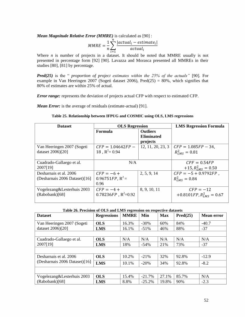
52
Mean Magnitude Relative Error (MMRE) is calculated as [90] :
∑
Where n is number of projects in a dataset. It should be noted that MMRE usually is not
presented in percentage form [92] [90]. Lavazza and Morasca presented all MMREs in their
studies [80], [81] by percentage.
Pred(25) is the ― proportion of project estimates within the 25% of the actuals” [90]. For
example in Van Heeringen 2007 (Sogeti dataset 2006), Pred(25) = 80%, which signifies that
80% of estimates are within 25% of actual.
Error range: represents the deviation of projects actual CFP with respect to estimated CFP.
Mean Error: is the average of residuals (estimate-actual) [91].
Table 25. Relationship between IFPUG and COSMIC using OLS, LMS regressions
Dataset OLS Regression LMS Regression Formula
Formula Outliers
Eliminated
projects
Van Heeringen 2007 (Sogeti
dataset 2006)[20] , R
2= 0.94
12, 11, 20, 23, 3 ,
Cuadrado-Gallaego et al.
2007[19]
N/A
Desharnais et al. 2006
(Desharnais 2006 Dataset)[16] , R
2 =
0.96
2, 5, 9, 14 ,
Vogelezang&Lesterhuis 2003
(Rabobank)[68] , R
2=0.92
8, 9, 10, 11
Table 26. Precision of OLS and LMS regression on respective datasets
Dataset Regressions MMRE Min Max Pred(25) Mean error
Van Heeringen 2007 (Sogeti
dataset 2006)[20] OLS 16.3% -30% 60% 84% -40.7
LMS 16.1% -51% 46% 88% -37
Cuadrado-Gallaego et al.
2007[19] OLS N/A N/A N/A N/A N/A
LMS 18% -54% 21% 73% -37
Desharnais et al. 2006
(Desharnais 2006 Dataset)[16] OLS 10.2% -21% 32% 92.8% -12.9
LMS 10.1% -20% 34% 92.8% -8.2
Vogelezang&Lesterhuis 2003
(Rabobank)[68] OLS 15.4% -21.7% 27.1% 85.7% N/A
LMS 8.8% -25.2% 19.8% 90% -2.3

53
Previous studies evaluated a conversion function between the two FP and COSMIC measures.
But it has been suggested that relationship might not be linear, since CFP increases more
proportionally than FP [81] and line‘s slope is increased for bigger projects [80]. In COSMIC
Advanced and Related Topics manual [56] it is stated that “summarizing the observations from
statistically-based size conversion studies, the true „average relationship‟ between IFPUG and
COSMIC scales should be a curve that starts „flatter‟ (i.e. IFPUG size is greater than COSMIC
size) but about 200 FP shows COSMIC sizes on average rising faster than IFPUG sizes”.
Before going into details of the approaches we should draw reader‘s attention to an important
point. This is true that setting a break point in the data set and deriving two separate formulas,
one for small projects and the other for big projects make the model non-linear. But it should be
noted that in regression analysis context these models are not called non-linear [93]. Lavazza
and Morasca used this term in their study [80] and named these models non-linear while in their
later study [81] they fixed this issue by using the correct term i.e. piecewise linear regression.
Here we use the name piecewise linear instead of name non-linear as other literature on
regression analysis. A piecewise linear regression curve is defined as ―a series of interconnected
segments‖ [81].
For the findings of the primary studies‘ results on piecewise regression, we presented formulas
as piecewise with and without removing outliers.
First Abran et al. [18] in their study identified that constant in first equation mentioned for
Vogelezang & Lesterhuis 2003 (Rabobank) [68] i.e. the intercept 87 is relatively high which
might be due to counting of logical files (ILF and EIF) in IFPUG which are not taken into count
during COSMIC measurement. They (Abran et al.) also stated that this formula is largely
affected by two big projects in dataset. This makes the formula inaccurate for small projects with
less than 200 NESMA points. So they split the datasets into two parts, one for projects less than
200 NESMA points (<=200) and other for larger projects (>200). The models obtained for these
two datasets are as follow:
( ) ( ) , R2 = 0.85 (NESMA <= 200)
( ) ( ) , R2 = 0.99 (NESMA > 200)
According to the COSMIC manual [56] for Van Heeringen 2007 dataset (Sogeti dataset 2006)
[20] following relations can be obtained:
( ) R2 = 0.45 (NESMA FP < 200 and 5 data points)
( ) ,R2 = 0.96 (NESMA FP < 200 and 21 data points)
Lavazza & Morasca [80] conducted their study in analyzing four datasets and compared the
results of linear models obtained by eliminating outliers and piecewise models obtained by
setting the discontinuity point. The results were compared in order to evaluate which is the best
representation of correlation between FP and CFP. There is no statistically significant evidence
to say that a dataset can be presented better by using piecewise regression. Both linear and
piecewise linear models have to be applied for the given datasets and see which can best present
relation between FP and CFP [80]. The results of this study [80] are shown in Table 27.

54
Table 27. Piecewise Linear Conversion without removing outliers for IFPUG and COSMIC
Dataset Authors Piecewise linear
formula
R2
Precision fitting Comments
MMRE Pred(25) Error
Range
Mean
Error
Vogelezang &
Lesterhuis 2003
(Rabobank)
[68]
Abran et
al. [18]
FP<=200,
( ) ( )
0.85 N/A N/A
FP>200, ( )
( ) –
0.99
Van Heeringen
2007 (Sogeti
dataset 2006)
[20]
Lavazza
[72] FP<=200, ( ) (5 data points)
0.45 N/A N/A
FP>200, ( ) ,
(21 data points)
0.96
Lavazza
[80] FP<=587, (16
data points)
0.95 15.5%
80%
N/A N/A Linear and piecewise
models are equivalent.
But piecewise linear
model is preferred as it
has more correct shape
compared to linear
model [80].
FP>586, (5
data points)
0.91
Cuadrado-
Gallaego et al.
2007 [19]
Lavazza
[80]
FP<250, (7
data points)
0.94 15.8% 75% -29%
..
46.5%
-5.5
CFP
Piecewise linear is the
only valid significant
model [80]
FP 250, (25
data points)
0.67
Desharnais et
al. 2006
(Desharnais
2006
Dataset)[16]
Lavazza
[80] FP<318, (7
data points)
0.96 N/A N/A N/A N/A Linear model is
applicable for this
dataset [80]
FP 318;
(7 data points)
0.92
Vogelezang &
Lesterhuis 2003
(Rabobank)
[68]
Lavazza
[80] FP<230, (6
data points)
0.94 26% 90% -20%
..
171%
16
CFP
Piecewise linear model
appears correct but is
worse than linear
model [80]. FP (4
data points)
0.95

55
Lavazza & Morasca [81] used piecewise linear models for the datasets which divides them into
two segments and a junction point is introduced. These models were derived by removing
outliers. In Table 28 we summarized the results of piecewise linear models [81].
Table 28. piecewise regression models with removing outliers for IFPUG and COSMIC conversions
Dataset
Piecewise Linear Regression Precision fitting
Conversion formula R2 Data points
& p value
MMRE Pred(25) Error
range
Mean
error
Cuadrado-
Gallaego et al.
2007 [19]
0.9342 10 data points,
2 outliers, p
value< 10-4
16.3% 71% -33 %
to
42%
-12
CFP
0.5429 24 data points
( 4 outliers) p
value=0.0001
4
Van
Heeringen
2007 (Sogeti
dataset 2006)
[20]
0.912 18 data points
(2 outliers), p
value< 10-4
16% 81% -30%
to
62%
-7
CFP
0.8965 8 data points
(3 outliers), p
value=0.0042
Desharnais et
al. 2006
(Desharnais
2006 Dataset)
[16]
0.9631 7 data points
(no outliers), p
value< 10-4
NA NA NA NA
0.8451 8 data points (
2 outliers)
p value=
0.0034
Luigi Lavazza in his study [5] explored quantitative relations between FPA BFC types and
COSMIC functional processes. He analyzed 25 projects of Van Heeringen 2007 (Sogeti dataset
2006) dataset and investigated the dependencies of FP and CFP from Base Function
Components perspective. Among 26 projects, project 17 is excluded since the data given in table
EI=EO=EQ=0 and ILF=3, EIF=2. This data was not reliable according to FPA rules. In addition
with Sogeti dataset Lavazza also derived a relation on Cuadrado-Gallaego et al. 2007 [19]
dataset. Table 29 summarizes the different correlations between FPA and COSMIC of Van
Heeringen 2007 (Sogeti dataset 2006) and only one correlation on Cuadrado-Gallaego et al.
2007 dataset.
Two statistics i.e. Average Absolute Error (AAE) and Estimation Error are used to test goodness
fit of the derived linear model. Average Absolute Error is calculated as follows:
∑ | | )
Where Y is predicted value and is absolute value and n represents number of projects in a
dataset.
Estimation error is calculated for each data point as:

56
Estimation Error =
In Table 29, in third column i.e. Estimation error, number of projects in dataset with estimation
error > 20% are represented.
Table 29. Correlation between FP and CFP BFC’s
Correlation
between
Formula R2
Average
Absolute
Error
(AAE)
Estimation
error
20% for
Project 19
Excluded
(Y/N)
1. CFP and FP 0.97 13.7% 6 projects
(one fourth)
Y
2.CFP and FP
BFC – 0.96 17.1% one third
projects
Y
0.94 17.5% 9 projects Y
0.98 15.5% 7 projects out
of 25
N
3.FP with non-
weighted FP
BFC
0.99 7.1% 3 projects N
(Cuadrado-
Gallaego et al. 2007 [19])
N/A N/A N/A N/A
4.FP and TF 0.96 11.7% 5 projects Y
5. FP with
elementary non
weighted FP
BFC
0.99 6.5% Only two cases N/A
6.COSMIC
functional
processes and
FP TF
0.97 14.2% 6 projects N
7.CFP and
COSMIC
functional
processes
0.96 18.6% 10 projects N/A
8. FP and
COSMIC
functional
processes
0.89 12.5% 5 projects Y
In most cases project 19 was excluded as it was small project with only 61 FP, which is half the
size of the second smallest project (129 FP). Inclusion of this project results in large variation
with respect to the derived linear model.
B.2 Non-Linear Regression based
This section discusses regression models derived from transformed datasets by log-log method.
Lavazza in his study [72] applied logarithmic transformations for four datasets and predicted the
power of them with help of some methods as shown in Table 30. Dataset of Cuadrado-Gallaego
et al. 2007[19] contains information on IFPUG and COSMIC measures but authors that provided
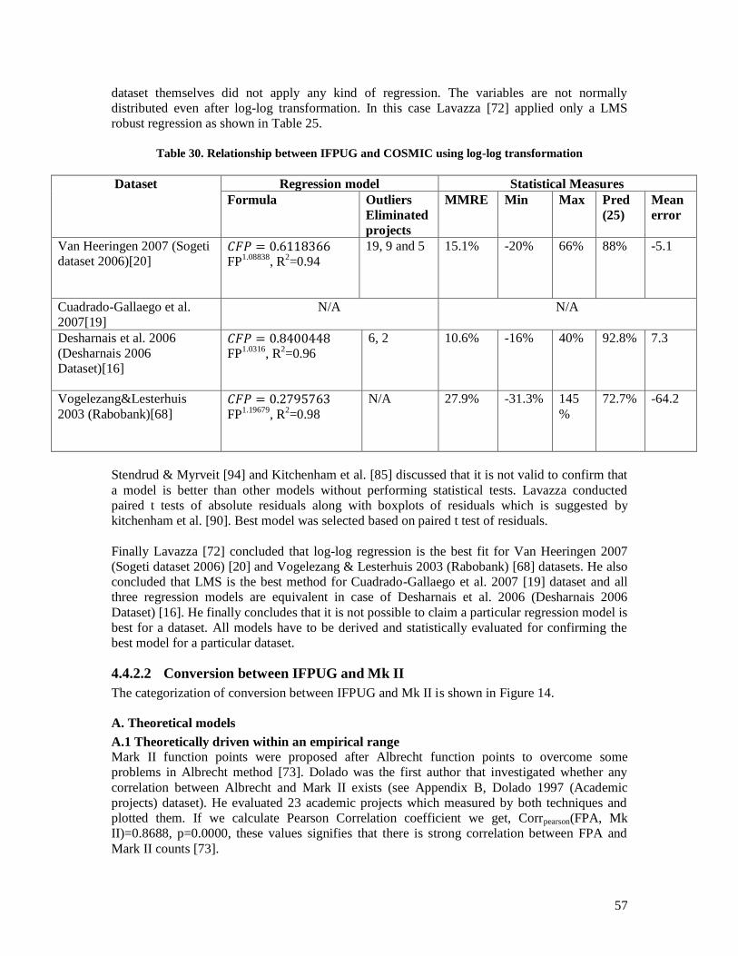
57
dataset themselves did not apply any kind of regression. The variables are not normally
distributed even after log-log transformation. In this case Lavazza [72] applied only a LMS
robust regression as shown in Table 25.
Table 30. Relationship between IFPUG and COSMIC using log-log transformation
Dataset Regression model Statistical Measures
Formula Outliers
Eliminated
projects
MMRE Min Max Pred
(25)
Mean
error
Van Heeringen 2007 (Sogeti
dataset 2006)[20] FP
1.08838, R
2=0.94
19, 9 and 5 15.1% -20% 66% 88% -5.1
Cuadrado-Gallaego et al.
2007[19]
N/A N/A
Desharnais et al. 2006
(Desharnais 2006
Dataset)[16]
FP
1.0316, R
2=0.96
6, 2 10.6% -16% 40% 92.8% 7.3
Vogelezang&Lesterhuis
2003 (Rabobank)[68]
FP1.19679
, R2=0.98
N/A 27.9% -31.3% 145
%
72.7% -64.2
Stendrud & Myrveit [94] and Kitchenham et al. [85] discussed that it is not valid to confirm that
a model is better than other models without performing statistical tests. Lavazza conducted
paired t tests of absolute residuals along with boxplots of residuals which is suggested by
kitchenham et al. [90]. Best model was selected based on paired t test of residuals.
Finally Lavazza [72] concluded that log-log regression is the best fit for Van Heeringen 2007
(Sogeti dataset 2006) [20] and Vogelezang & Lesterhuis 2003 (Rabobank) [68] datasets. He also
concluded that LMS is the best method for Cuadrado-Gallaego et al. 2007 [19] dataset and all
three regression models are equivalent in case of Desharnais et al. 2006 (Desharnais 2006
Dataset) [16]. He finally concludes that it is not possible to claim a particular regression model is
best for a dataset. All models have to be derived and statistically evaluated for confirming the
best model for a particular dataset.
4.4.2.2 Conversion between IFPUG and Mk II
The categorization of conversion between IFPUG and Mk II is shown in Figure 14.
A. Theoretical models
A.1 Theoretically driven within an empirical range
Mark II function points were proposed after Albrecht function points to overcome some
problems in Albrecht method [73]. Dolado was the first author that investigated whether any
correlation between Albrecht and Mark II exists (see Appendix B, Dolado 1997 (Academic
projects) dataset). He evaluated 23 academic projects which measured by both techniques and
plotted them. If we calculate Pearson Correlation coefficient we get, Corrpearson(FPA, Mk
II)=0.8688, p=0.0000, these values signifies that there is strong correlation between FPA and
Mark II counts [73].
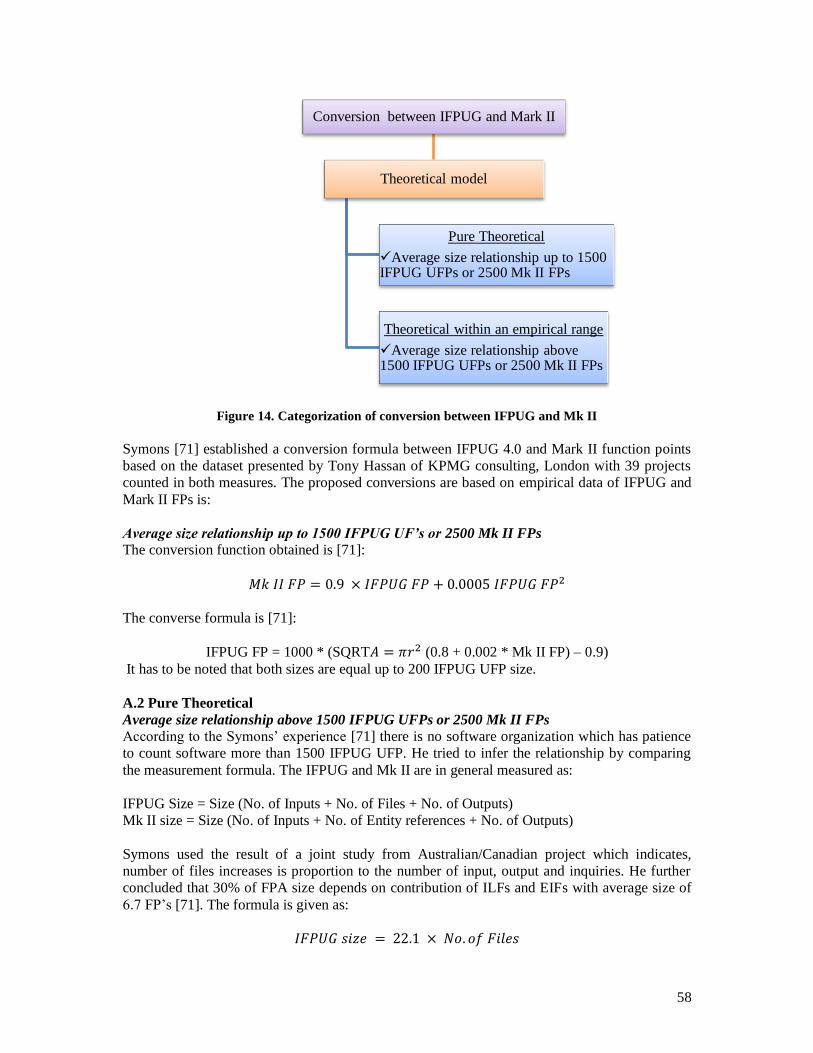
58
Figure 14. Categorization of conversion between IFPUG and Mk II
Symons [71] established a conversion formula between IFPUG 4.0 and Mark II function points
based on the dataset presented by Tony Hassan of KPMG consulting, London with 39 projects
counted in both measures. The proposed conversions are based on empirical data of IFPUG and
Mark II FPs is:
Average size relationship up to 1500 IFPUG UF’s or 2500 Mk II FPs
The conversion function obtained is [71]:
The converse formula is [71]:
IFPUG FP = 1000 * (SQRT (0.8 + 0.002 * Mk II FP) – 0.9)
It has to be noted that both sizes are equal up to 200 IFPUG UFP size.
A.2 Pure Theoretical
Average size relationship above 1500 IFPUG UFPs or 2500 Mk II FPs
According to the Symons‘ experience [71] there is no software organization which has patience
to count software more than 1500 IFPUG UFP. He tried to infer the relationship by comparing
the measurement formula. The IFPUG and Mk II are in general measured as:
IFPUG Size = Size (No. of Inputs + No. of Files + No. of Outputs)
Mk II size = Size (No. of Inputs + No. of Entity references + No. of Outputs)
Symons used the result of a joint study from Australian/Canadian project which indicates,
number of files increases is proportion to the number of input, output and inquiries. He further
concluded that 30% of FPA size depends on contribution of ILFs and EIFs with average size of
6.7 FP‘s [71]. The formula is given as:
Conversion between IFPUG and Mark II
Theoretical model
Pure Theoretical
Average size relationship up to 1500 IFPUG UFPs or 2500 Mk II FPs
Theoretical within an empirical range
Average size relationship above 1500 IFPUG UFPs or 2500 Mk II FPs
59
Similarly for Mk II, the entity references contribute 46.75% of total Mark II FP size with an
average of 1.66 FPs.
Finally the ratio of sizes for two large systems is [71]:
T.Kralj et al. [74] established relation between base elements of IFPUG FPA and Mk II as
follows:
No. of DETs (IFPUG FPA) = [input data + output data] (Mk II FPA)
No. of FTRs (IFPUG FPA) = No. of referenced entities (Mk II FPA)
60
5 RELIABILITY OF CONVERSION APPROACHES From here the focus of our study in the scope of this thesis is on the conversion between two
widely used FSM methods; IFPUG and COSMIC.
We can divide proposed regression models into three categories: Linear models, piecewise linear
models, and non-linear models. Some of these equations are derived from distinct datasets and
some are derived from previous datasets by removing outliers or removing unreliable data.
Outliers are those data having Cook‘s Distance [89] bigger than 4/n where n is total number of
data points. In addition data points with standardized residual [93] bigger than 2 or less than -2,
are considered as outliers as well. Unreliable data are those data that authors had doubt regarding
their correctness. Doubts can be about reliability of measure or correctness of measured value
etc. All of the equations and the associated dataset(s) were discussed in previous section.
Before going into detail of each method and finding their weak points and evaluating their
reliability we think it is necessary to give to the reader a summary of regression techniques.
After this summary we improve one of the techniques (piecewise linear regression) by making it
systematic and rigorous. Indeed this improvement helps to handle problem of finding
discontinuity point for that regression technique. We used Rabobank dataset (see Appendix B) as
a sample for describing each approach.
5.1 Regression Techniques Already Used in Conversion
5.1.1 Linear Regression To establish a relation between a response variable and several predictors one way is to use
regression analysis to build a regression model [95]. In our case i.e. convertibility of IFPUG to
COSMIC, literature takes COSMIC as response variable and IFPUG is the only predictor.
Resulting equation is in the following form:
CFP = A × FP + B
A is called slope and B is intercept. One important characteristic of regression models is R2
value (Pronounced R Squared). R2 is called coefficient of determination and shows the goodness
of fit or how well regression model fits the data that were used to build it [84]. Value of R2 is
ranged from 0 to 1. The closer value to 1 the better the fitness to data. As an example, Figure 15
shows scatter plot for Rabobank dataset. Regression line has the following formula:
CFP = 1.201 × FP – 86.815
R2 value is 0.9856
This R2 value shows a good fitness over the data. This approach to perform linear regression is
called OLS (Ordinary Least Squares). That means an equation is derived by ―minimizing equally
weighted sum of squares of residuals‖ [93].
5.1.2 Piecewise Linear Regression There are cases that not all data points follow a single linear model and the model can be
presented better by dividing the predictor variable‘s range into pieces. In the context of
convertibility between IFPUG and COSMIC Abran [18] in study of Rabobank dataset suggested
that it is better to make a linear model for projects having less than 200 FP and another linear
model for project with FP value greater than 200 FP.

61
For less than 200 FP equation is:
CFP = 0.75 × FP – 2.6
R2 is 0.85 for the first part.
For projects with FP bigger than 200, formula is:
CFP = 1.2 × FP - 108
R2 for second part is 0.99.
Figure 16 shows piecewise linear regression on the Rabobank dataset.
5.1.3 Robust Regression Models One drawback in using OLS regression method is its sensitivity to outliers [86]. Although it is
possible to remove outliers to make dataset more homogenous, not always this approach pays
off. This is because sometimes outliers are natural in a dataset and their presence is not due to
measurement mistakes. To overcome this issue other approaches like LMS (Least Median of
Squares) are proposed [86] and used [72] in building models. Figure 17shows Rabobank dataset
with LMS regression line. Formula for this model is:
CFP = 0.8121 × FP – 12
Here R2 is 0.67.
5.1.4 Non-linear Models In the context of convertibility between IFPUG and COSMIC, Lavazza [72] applied log-log
transformation on different datasets. Log-log transformation transforms data points in a dataset
to their corresponding logarithm value to make data more linear. After this an OLS regression is
performed on transformed model and the resulting formula is converted to non-linear form to be
applicable for original data. Figure 18 depicts Rabobank dataset with a non-linear line derived
from log-log transformed dataset. Here the formula is as:
CFP = 0.2795 × FP 1.19679
R2 value for this model is 0.98.

62
Figure 15. Scatter plot of Rabobank dataset with an OLS regression line
Figure 16. Scatterplot of Rabobank dataset with two linear lines; less than 200 FP (Blue line) and
bigger than 200 FP (Red line)

63
Figure 17. Scatterplot of Rabobank dataset with LMS regression line
Figure 18. Scatterplot of Rabobank dataset with regression equation after log-log transformation
64
5.2 An Improvement Suggestion for Systematically Handling
Discontinuity Point in COSMIC-IFPUG Relationship Abran et al. [18] in their study of Function Points to COSMIC suggested that if we split
Rabobank dataset into two parts i.e. less than 200 FP and greater than 200 FP, conversion
formula will work better. They didn‘t provide any clue that how they derived this 200 FP.
COSMIC took the idea of Abran et al. and in COSMIC Manual [28], this is also stated that it is
better to divide each dataset into small and large projects. Discontinuity point in COSMIC
manual is also 200 based on Abran et al. [18].
After them Lavazza and Morasca also studied piecewise liner regression in their two studies
[80], [81]. Title of first study [80] is quite misleading. Paper is titled ―A Study of Non-linearity
in the Statistical Convertibility of Function Points into COSMIC Function Points‖, while the
only studied topic is piecewise linear regression, the word ―Non-linearity‖ brings other meanings
into the mind. In this study also there is no systematic approach for finding break point to divide
dataset into to partitions. The latter [81], has corrected the problem in the title but again there is
no systematic approach for finding discontinuity point. It is mentioned in the paper that authors
used a systematic way to form two separate models and calculate model characteristics like R2
value but there is no notion of approach for finding discontinuity point. Also the sentence ―it is
quite improbable that our choice leads to missing any particularly interesting junction point‖
mean there is a chance (even very small) that we miss some interesting points. Our results (as
stated in Table 31) based on systematic approach also show that they really missed interesting
points.
To improve these approaches and to make a systematic and repeatable algorithm for finding best
discontinuity point we developed an a procedure and implemented it in a Java program (source
code available upon request) to find best discontinuity point with 100% confidence that we don‘t
lose any point and the point found by program is always the best possible choice. The procedure
is as follows:
1. Sort the dataset in ascending order based on FP.
2. Start by setting a minimum size for each sub dataset, for instance at least each part
should have 5 points in it.
3. Take the first five point of dataset as first part and rest of data points as second part of
model.
4. Remove outliers based on Cook‘s distance [93] and standardized residual for both first
and second part. Data points with Cook‘s distance larger than 4 / n which n is total
number of data in each part will be removed. Data points with absolute value of
standardized residual larger than or equal to 2 will be also removed.
5. After removing outliers, if size of either of models reach below minimum size we throw
away discontinuity point and go to Step 8.
6. Make OLS model for both parts.
7. Calculate R2, MMRE and Pred(25) based on the formula derived from model and store
them.
8. Remove the first data point in second part and add it to first part to come with two new
first part and second part.
9. If size of second part is below the minimum size stop the procedure and go to Step 11.
10. Go to Step 4.
11. Among saved list of R2, MMRE and Pred(25) we can find the best combination i.e.
tradeoff between minimum MMRE and Maximum Pred(25).
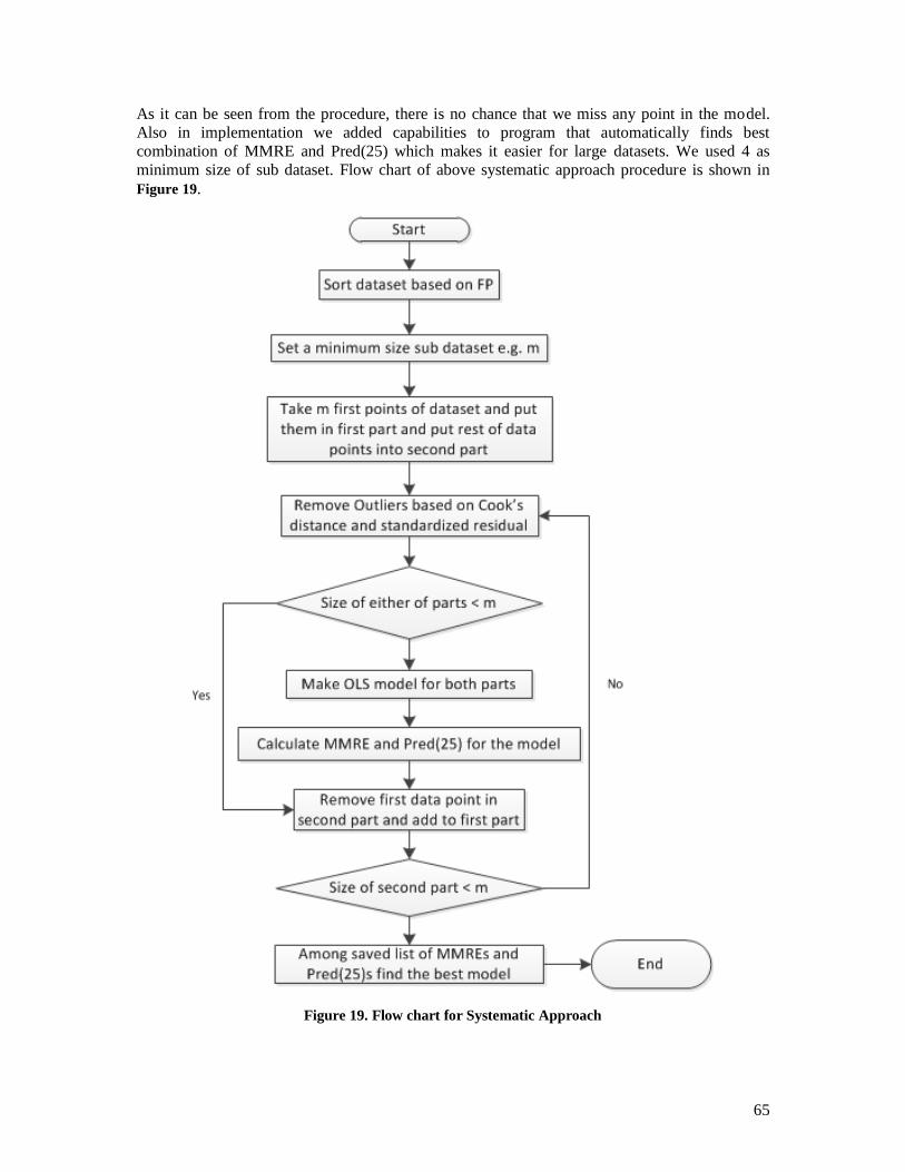
65
As it can be seen from the procedure, there is no chance that we miss any point in the model.
Also in implementation we added capabilities to program that automatically finds best
combination of MMRE and Pred(25) which makes it easier for large datasets. We used 4 as
minimum size of sub dataset. Flow chart of above systematic approach procedure is shown in
Figure 19.
Figure 19. Flow chart for Systematic Approach
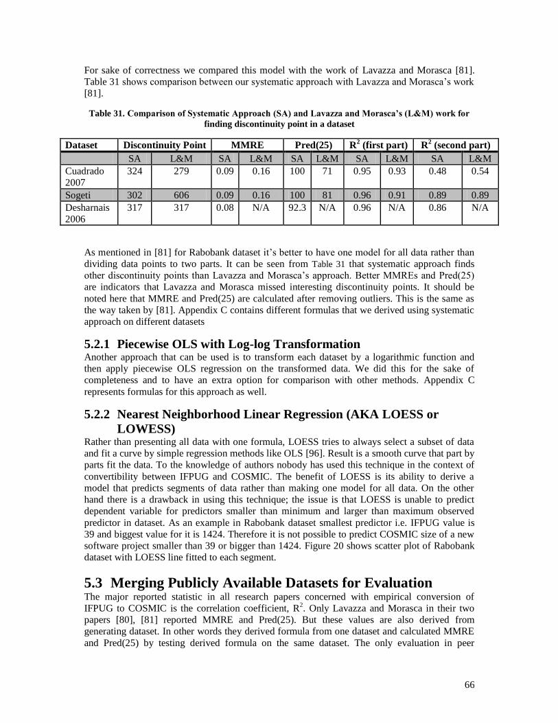
66
For sake of correctness we compared this model with the work of Lavazza and Morasca [81].
Table 31 shows comparison between our systematic approach with Lavazza and Morasca‘s work
[81].
Table 31. Comparison of Systematic Approach (SA) and Lavazza and Morasca’s (L&M) work for
finding discontinuity point in a dataset
Dataset Discontinuity Point MMRE Pred(25) R2 (first part) R
2 (second part)
SA L&M SA L&M SA L&M SA L&M SA L&M
Cuadrado
2007
324 279 0.09 0.16 100 71 0.95 0.93 0.48 0.54
Sogeti 302 606 0.09 0.16 100 81 0.96 0.91 0.89 0.89
Desharnais
2006
317 317 0.08 N/A 92.3 N/A 0.96 N/A 0.86 N/A
As mentioned in [81] for Rabobank dataset it‘s better to have one model for all data rather than
dividing data points to two parts. It can be seen from Table 31 that systematic approach finds
other discontinuity points than Lavazza and Morasca‘s approach. Better MMREs and Pred(25)
are indicators that Lavazza and Morasca missed interesting discontinuity points. It should be
noted here that MMRE and Pred(25) are calculated after removing outliers. This is the same as
the way taken by [81]. Appendix C contains different formulas that we derived using systematic
approach on different datasets
5.2.1 Piecewise OLS with Log-log Transformation Another approach that can be used is to transform each dataset by a logarithmic function and
then apply piecewise OLS regression on the transformed data. We did this for the sake of
completeness and to have an extra option for comparison with other methods. Appendix C
represents formulas for this approach as well.
5.2.2 Nearest Neighborhood Linear Regression (AKA LOESS or
LOWESS) Rather than presenting all data with one formula, LOESS tries to always select a subset of data
and fit a curve by simple regression methods like OLS [96]. Result is a smooth curve that part by
parts fit the data. To the knowledge of authors nobody has used this technique in the context of
convertibility between IFPUG and COSMIC. The benefit of LOESS is its ability to derive a
model that predicts segments of data rather than making one model for all data. On the other
hand there is a drawback in using this technique; the issue is that LOESS is unable to predict
dependent variable for predictors smaller than minimum and larger than maximum observed
predictor in dataset. As an example in Rabobank dataset smallest predictor i.e. IFPUG value is
39 and biggest value for it is 1424. Therefore it is not possible to predict COSMIC size of a new
software project smaller than 39 or bigger than 1424. Figure 20 shows scatter plot of Rabobank
dataset with LOESS line fitted to each segment.
5.3 Merging Publicly Available Datasets for Evaluation The major reported statistic in all research papers concerned with empirical conversion of
IFPUG to COSMIC is the correlation coefficient, R2. Only Lavazza and Morasca in their two
papers [80], [81] reported MMRE and Pred(25). But these values are also derived from
generating dataset. In other words they derived formula from one dataset and calculated MMRE
and Pred(25) by testing derived formula on the same dataset. The only evaluation in peer
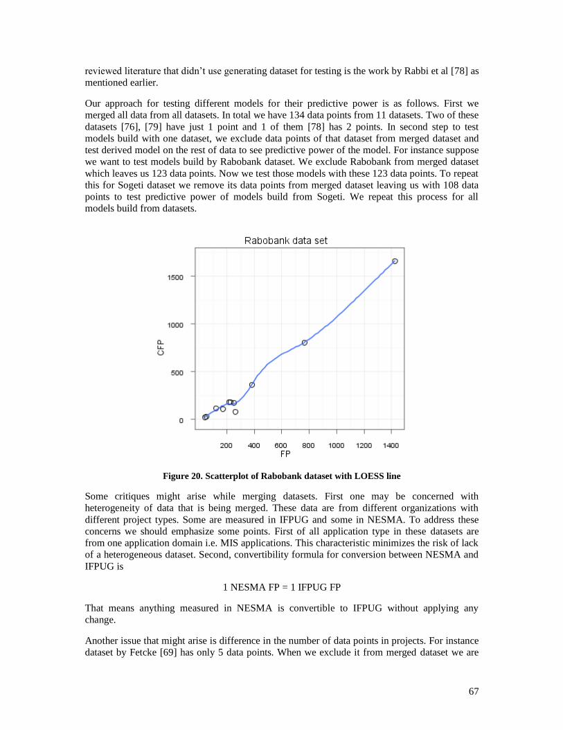
67
reviewed literature that didn‘t use generating dataset for testing is the work by Rabbi et al [78] as
mentioned earlier.
Our approach for testing different models for their predictive power is as follows. First we
merged all data from all datasets. In total we have 134 data points from 11 datasets. Two of these
datasets [76], [79] have just 1 point and 1 of them [78] has 2 points. In second step to test
models build with one dataset, we exclude data points of that dataset from merged dataset and
test derived model on the rest of data to see predictive power of the model. For instance suppose
we want to test models build by Rabobank dataset. We exclude Rabobank from merged dataset
which leaves us 123 data points. Now we test those models with these 123 data points. To repeat
this for Sogeti dataset we remove its data points from merged dataset leaving us with 108 data
points to test predictive power of models build from Sogeti. We repeat this process for all
models build from datasets.
Figure 20. Scatterplot of Rabobank dataset with LOESS line
Some critiques might arise while merging datasets. First one may be concerned with
heterogeneity of data that is being merged. These data are from different organizations with
different project types. Some are measured in IFPUG and some in NESMA. To address these
concerns we should emphasize some points. First of all application type in these datasets are
from one application domain i.e. MIS applications. This characteristic minimizes the risk of lack
of a heterogeneous dataset. Second, convertibility formula for conversion between NESMA and
IFPUG is
1 NESMA FP = 1 IFPUG FP
That means anything measured in NESMA is convertible to IFPUG without applying any
change.
Another issue that might arise is difference in the number of data points in projects. For instance
dataset by Fetcke [69] has only 5 data points. When we exclude it from merged dataset we are
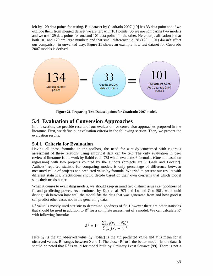
68
left by 129 data points for testing. But dataset by Cuadrado 2007 [19] has 33 data point and if we
exclude them from merged dataset we are left with 101 points. So we are comparing two models
and we use 129 data points for one and 101 data points for the other. Here our justification is that
both 101 and 129 are large numbers and that small difference i.e. 28 (129 – 101) doesn‘t affect
our comparison in unwanted way. Figure 21 shows an example how test dataset for Cuadrado
2007 models is derived.
Figure 21. Preparing Test Dataset points for Cuadrado 2007 models
5.4 Evaluation of Conversion Approaches In this section, we provide results of our evaluation for conversion approaches proposed in the
literature. First, we define our evaluation criteria in the following section. Then, we present the
evaluation results.
5.4.1 Criteria for Evaluation Having all these formulas in the toolbox, the need for a study concerned with rigorous
assessment of these relations using empirical data can be felt. The only evaluation in peer
reviewed literature is the work by Rabbi et al [78] which evaluates 6 formulas (One not based on
regression) with two projects counted by the authors (projects are PCGeek and Locator).
Authors‘ reported statistic for comparing models is only percentage of difference between
measured value of projects and predicted value by formula. We tried to present our results with
different statistics. Practitioners should decide based on their own concerns that which model
suits their needs better.
When it comes to evaluating models, we should keep in mind two distinct issues i.e. goodness of
fit and predicting power. As mentioned by Kok et al [97] and Lo and Gao [98], we should
distinguish between how well the model fits the data that was generated from and how good it
can predict other cases not in the generating data.
R2 value is mostly used statistic to determine goodness of fit. However there are other statistics
that should be used in addition to R2 for a complete assessment of a model. We can calculate R
2
with following formula:
∑ ( )
∑ ( )
Here is the kth observed value, (x-hat) is the kth predicted value and is mean for n
observed values. R2 ranges between 0 and 1. The closer R2 to 1 the better model fits the data. It
should be noted that R2 is valid for model built by Ordinary Least Squares [99]. There is not a

69
certain point for decision to say if for a model R2 is greater than that number then that model is
good, unless it is bad. It is suggested that if R2 is bigger than 0.5 the model has good power in
explaining its data [81].
MMRE (Mean Magnitude of Relative Error) and Pred(m) (count of the number of predictions
within m% of actuals) are two widely used statistics to measure accuracy of prediction models in
software engineering [91]. According to Conte et al [100] in the absence of any generally
accepted standard MMRE and Pred(25) seem most suitable statistics as prediction quality
indicators. MMRE is calculated based on following formula:
∑
There are other statistics as well that each play specific role in assessment of different models.
To evaluate models we used a combination of different statistics suggested by literature
[101][91][98]. One of those statistics suggested by Kitchenham [91] is variable z defined as:
We can compare boxplots of z variable for all models to see which model yields a better result.
Better models result in boxplots of z with shorter box length, less outliers and median line close
to 1. Use of boxplot cannot say anything about statistically significance of model, in this case it
is strongly recommended that we use a statistical test like paired t test suggested by Kitchenham
et al [91]. However since in our case our distribution of z is not normal, we should use non-
parametric methods like Mann-Whitney test [102] to compare medians for different models. In
practice Mann-Whitney test didn‘t find any significant difference between most of methods, so
we didn‘t report those results here.
Another straightforward and useful statistic that we use is e or error defined by:
Again we can compare boxplot of e for different models to see which works better in terms of
shorter length of boxplots and closer medians to 0.
As final note it should be noted that MMRE and Pred(n) are indicators of skewness and kurtosis
of relative error random variable respectively [91], [99].
5.4.2 Evaluation Results From here for the sake of brevity we use a code for each method and author. Tables describing
dataset code, author code, and method code are Table 32, Table 33 and Table 34 respectively.
Formula ID is coded as XXYYZ. XX represents dataset code, YY author(s) code and finally Z
method number. Since models in the literature are derived from single datasets we evaluated
models proposed for each dataset along with our own methods applied on the same dataset.
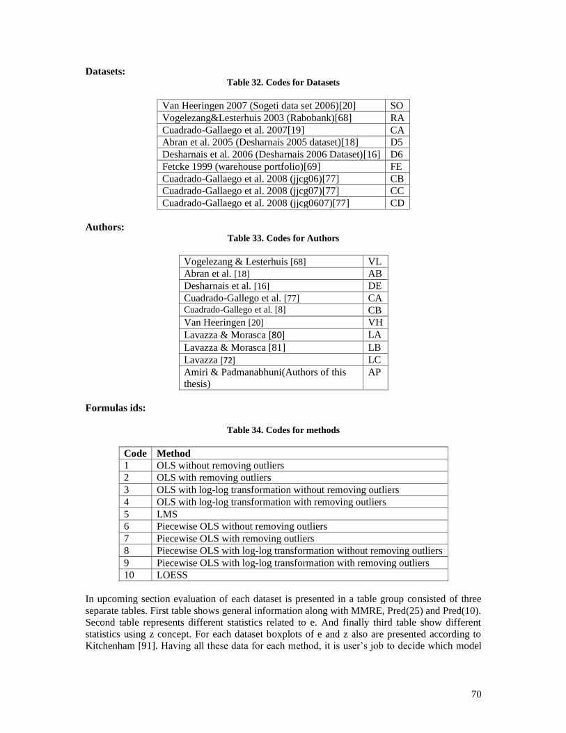
70
Datasets: Table 32. Codes for Datasets
Van Heeringen 2007 (Sogeti data set 2006)[20] SO
Vogelezang&Lesterhuis 2003 (Rabobank)[68] RA
Cuadrado-Gallaego et al. 2007[19] CA
Abran et al. 2005 (Desharnais 2005 dataset)[18] D5
Desharnais et al. 2006 (Desharnais 2006 Dataset)[16] D6
Fetcke 1999 (warehouse portfolio)[69] FE
Cuadrado-Gallaego et al. 2008 (jjcg06)[77] CB
Cuadrado-Gallaego et al. 2008 (jjcg07)[77] CC
Cuadrado-Gallaego et al. 2008 (jjcg0607)[77] CD
Authors: Table 33. Codes for Authors
Vogelezang & Lesterhuis [68] VL
Abran et al. [18] AB
Desharnais et al. [16] DE
Cuadrado-Gallego et al. [77] CA Cuadrado-Gallego et al. [8] CB
Van Heeringen [20] VH
Lavazza & Morasca [80] LA
Lavazza & Morasca [81] LB
Lavazza [72] LC
Amiri & Padmanabhuni(Authors of this
thesis)
AP
Formulas ids:
Table 34. Codes for methods
Code Method
1 OLS without removing outliers
2 OLS with removing outliers
3 OLS with log-log transformation without removing outliers
4 OLS with log-log transformation with removing outliers
5 LMS
6 Piecewise OLS without removing outliers
7 Piecewise OLS with removing outliers
8 Piecewise OLS with log-log transformation without removing outliers
9 Piecewise OLS with log-log transformation with removing outliers
10 LOESS
In upcoming section evaluation of each dataset is presented in a table group consisted of three
separate tables. First table shows general information along with MMRE, Pred(25) and Pred(10).
Second table represents different statistics related to e. And finally third table show different
statistics using z concept. For each dataset boxplots of e and z also are presented according to
Kitchenham [91]. Having all these data for each method, it is user‘s job to decide which model
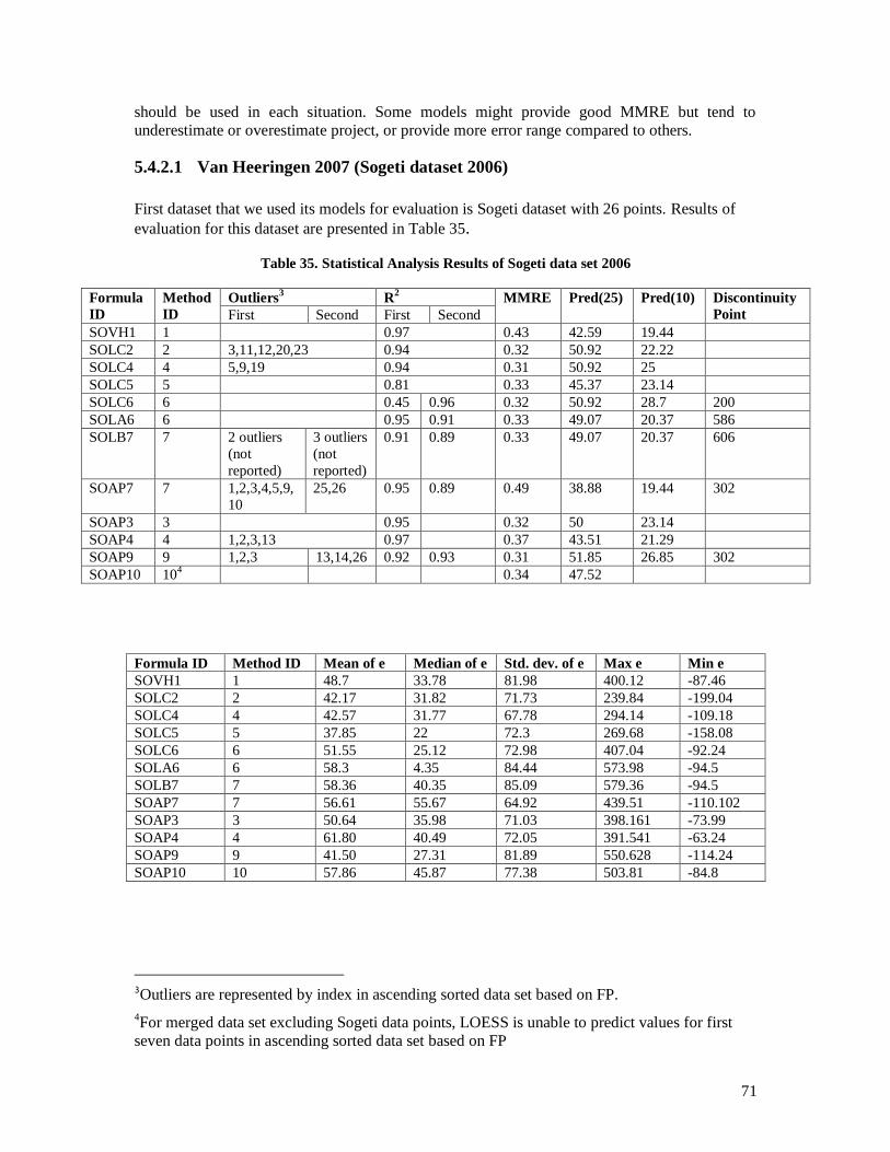
71
should be used in each situation. Some models might provide good MMRE but tend to
underestimate or overestimate project, or provide more error range compared to others.
5.4.2.1 Van Heeringen 2007 (Sogeti dataset 2006)
First dataset that we used its models for evaluation is Sogeti dataset with 26 points. Results of
evaluation for this dataset are presented in Table 35.
Table 35. Statistical Analysis Results of Sogeti data set 2006
Formula
ID
Method
ID
Outliers3 R
2 MMRE Pred(25) Pred(10) Discontinuity
Point First Second First Second
SOVH1 1 0.97 0.43 42.59 19.44
SOLC2 2 3,11,12,20,23 0.94 0.32 50.92 22.22
SOLC4 4 5,9,19 0.94 0.31 50.92 25
SOLC5 5 0.81 0.33 45.37 23.14
SOLC6 6 0.45 0.96 0.32 50.92 28.7 200
SOLA6 6 0.95 0.91 0.33 49.07 20.37 586
SOLB7 7 2 outliers
(not
reported)
3 outliers
(not
reported)
0.91 0.89 0.33 49.07 20.37 606
SOAP7 7 1,2,3,4,5,9,
10
25,26 0.95 0.89 0.49 38.88 19.44 302
SOAP3 3 0.95 0.32 50 23.14
SOAP4 4 1,2,3,13 0.97 0.37 43.51 21.29
SOAP9 9 1,2,3 13,14,26 0.92 0.93 0.31 51.85 26.85 302
SOAP10 104 0.34 47.52
Formula ID Method ID Mean of e Median of e Std. dev. of e Max e Min e
SOVH1 1 48.7 33.78 81.98 400.12 -87.46
SOLC2 2 42.17 31.82 71.73 239.84 -199.04
SOLC4 4 42.57 31.77 67.78 294.14 -109.18
SOLC5 5 37.85 22 72.3 269.68 -158.08
SOLC6 6 51.55 25.12 72.98 407.04 -92.24
SOLA6 6 58.3 4.35 84.44 573.98 -94.5
SOLB7 7 58.36 40.35 85.09 579.36 -94.5
SOAP7 7 56.61 55.67 64.92 439.51 -110.102
SOAP3 3 50.64 35.98 71.03 398.161 -73.99
SOAP4 4 61.80 40.49 72.05 391.541 -63.24
SOAP9 9 41.50 27.31 81.89 550.628 -114.24
SOAP10 10 57.86 45.87 77.38 503.81 -84.8
3Outliers are represented by index in ascending sorted data set based on FP.
4For merged data set excluding Sogeti data points, LOESS is unable to predict values for first
seven data points in ascending sorted data set based on FP
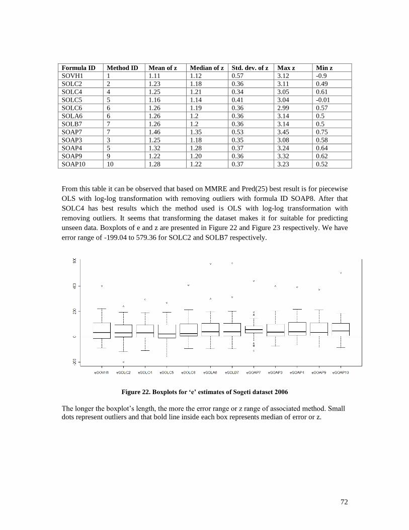
72
Formula ID Method ID Mean of z Median of z Std. dev. of z Max z Min z
SOVH1 1 1.11 1.12 0.57 3.12 -0.9
SOLC2 2 1.23 1.18 0.36 3.11 0.49
SOLC4 4 1.25 1.21 0.34 3.05 0.61
SOLC5 5 1.16 1.14 0.41 3.04 -0.01
SOLC6 6 1.26 1.19 0.36 2.99 0.57
SOLA6 6 1.26 1.2 0.36 3.14 0.5
SOLB7 7 1.26 1.2 0.36 3.14 0.5
SOAP7 7 1.46 1.35 0.53 3.45 0.75
SOAP3 3 1.25 1.18 0.35 3.08 0.58
SOAP4 5 1.32 1.28 0.37 3.24 0.64
SOAP9 9 1.22 1.20 0.36 3.32 0.62
SOAP10 10 1.28 1.22 0.37 3.23 0.52
From this table it can be observed that based on MMRE and Pred(25) best result is for piecewise
OLS with log-log transformation with removing outliers with formula ID SOAP8. After that
SOLC4 has best results which the method used is OLS with log-log transformation with
removing outliers. It seems that transforming the dataset makes it for suitable for predicting
unseen data. Boxplots of e and z are presented in Figure 22 and Figure 23 respectively. We have
error range of -199.04 to 579.36 for SOLC2 and SOLB7 respectively.
Figure 22. Boxplots for ‘e’ estimates of Sogeti dataset 2006
The longer the boxplot‘s length, the more the error range or z range of associated method. Small
dots represent outliers and that bold line inside each box represents median of error or z.
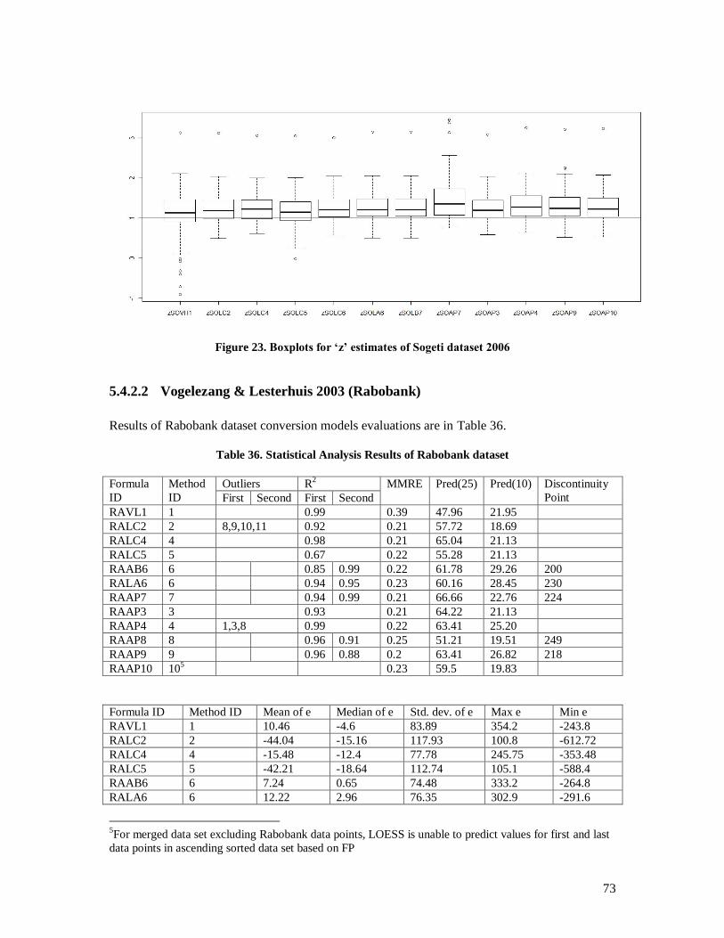
73
Figure 23. Boxplots for ‘z’ estimates of Sogeti dataset 2006
5.4.2.2 Vogelezang & Lesterhuis 2003 (Rabobank)
Results of Rabobank dataset conversion models evaluations are in Table 36.
Table 36. Statistical Analysis Results of Rabobank dataset
Formula
ID
Method
ID
Outliers R2 MMRE Pred(25) Pred(10) Discontinuity
Point First Second First Second
RAVL1 1 0.99 0.39 47.96 21.95
RALC2 2 8,9,10,11 0.92 0.21 57.72 18.69
RALC4 4 0.98 0.21 65.04 21.13
RALC5 5 0.67 0.22 55.28 21.13
RAAB6 6 0.85 0.99 0.22 61.78 29.26 200
RALA6 6 0.94 0.95 0.23 60.16 28.45 230
RAAP7 7 0.94 0.99 0.21 66.66 22.76 224
RAAP3 3 0.93 0.21 64.22 21.13
RAAP4 4 1,3,8 0.99 0.22 63.41 25.20
RAAP8 8 0.96 0.91 0.25 51.21 19.51 249
RAAP9 9 0.96 0.88 0.2 63.41 26.82 218
RAAP10 105 0.23 59.5 19.83
Formula ID Method ID Mean of e Median of e Std. dev. of e Max e Min e
RAVL1 1 10.46 -4.6 83.89 354.2 -243.8
RALC2 2 -44.04 -15.16 117.93 100.8 -612.72
RALC4 4 -15.48 -12.4 77.78 245.75 -353.48
RALC5 5 -42.21 -18.64 112.74 105.1 -588.4
RAAB6 6 7.24 0.65 74.48 333.2 -264.8
RALA6 6 12.22 2.96 76.35 302.9 -291.6
5For merged data set excluding Rabobank data points, LOESS is unable to predict values for first and last
data points in ascending sorted data set based on FP
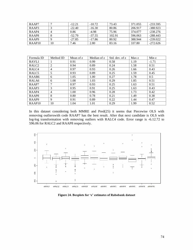
74
RAAP7 7 -12.21 -10.72 73.43 371.055 -233.595
RAAP3 3 -22.40 -16.30 80.86 206.917 -388.923
RAAP4 4 0.86 -4.98 75.96 374.077 -238.276
RAAP8 8 -52.79 -37.55 102.91 596.063 -288.443
RAAP9 9 -27.85 -17.86 80.92 388.944 -239.022
RAAP10 10 7.46 2.80 83.16 337.80 -272.626
Formula ID Method ID Mean of z Median of z Std. dev. of z Max z Min z
RAVL1 1 0.91 0.99 0.58 1.19 -1.71
RALC2 2 0.94 0.89 0.24 1.58 0.51
RALC4 4 0.97 0.93 0.26 1.66 0.43
RALC5 5 0.93 0.89 0.25 1.59 0.45
RAAB6 6 1.05 1.00 0.27 1.78 0.5
RALA6 6 1.08 1.03 0.29 1.85 0.51
RAAP7 7 0.97 0.93 0.25 1.63 0.51
RAAP3 3 0.95 0.91 0.25 1.63 0.43
RAAP4 4 1.00 0.96 0.28 1.73 0.42
RAAP8 8 0.80 0.78 0.21 1.49 0.38
RAAP9 9 0.91 0.89 0.22 1.44 0.47
RAAP10 10 1.04 1.01 0.29 1.99 0.52
In this dataset considering both MMRE and Pred(25) it seems that Piecewise OLS with
removing outlierswith code RAAP7 has the best result. After that next candidate is OLS with
log-log transformation with removing outliers with RALC4 code. Error range is -6.12.72 to
596.06 for RALC2 and RAAP8 respectively.
Figure 24. Boxplots for ‘e’ estimates of Rabobank dataset
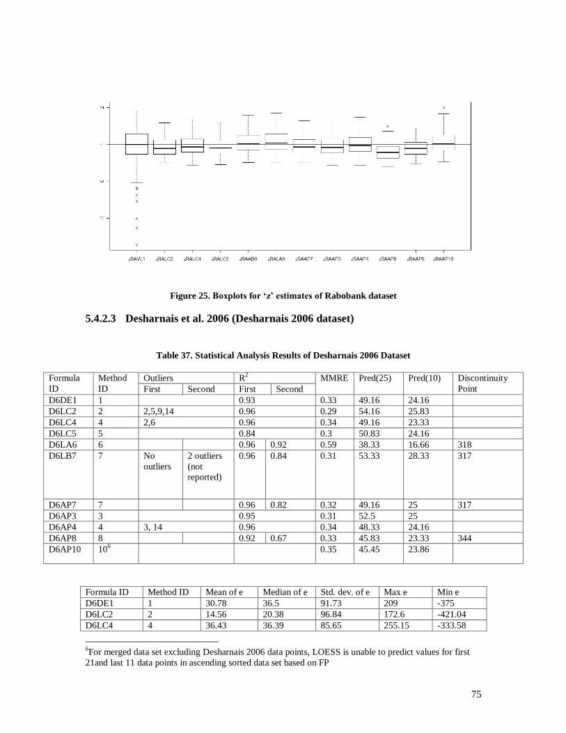
75
Figure 25. Boxplots for ‘z’ estimates of Rabobank dataset
5.4.2.3 Desharnais et al. 2006 (Desharnais 2006 dataset)
Table 37. Statistical Analysis Results of Desharnais 2006 Dataset
Formula
ID
Method
ID
Outliers R2 MMRE Pred(25) Pred(10) Discontinuity
Point First Second First Second
D6DE1 1 0.93 0.33 49.16 24.16
D6LC2 2 2,5,9,14 0.96 0.29 54.16 25.83
D6LC4 4 2,6 0.96 0.34 49.16 23.33
D6LC5 5 0.84 0.3 50.83 24.16
D6LA6 6 0.96 0.92 0.59 38.33 16.66 318
D6LB7 7 No
outliers
2 outliers
(not
reported)
0.96 0.84 0.31 53.33 28.33 317
D6AP7 7 0.96 0.82 0.32 49.16 25 317
D6AP3 3 0.95 0.31 52.5 25
D6AP4 4 3, 14 0.96 0.34 48.33 24.16
D6AP8 8 0.92 0.67 0.33 45.83 23.33 344
D6AP10 106 0.35 45.45 23.86
Formula ID Method ID Mean of e Median of e Std. dev. of e Max e Min e
D6DE1 1 30.78 36.5 91.73 209 -375
D6LC2 2 14.56 20.38 96.84 172.6 -421.04
D6LC4 4 36.43 36.39 85.65 255.15 -333.58
6For merged data set excluding Desharnais 2006 data points, LOESS is unable to predict values for first
21and last 11 data points in ascending sorted data set based on FP
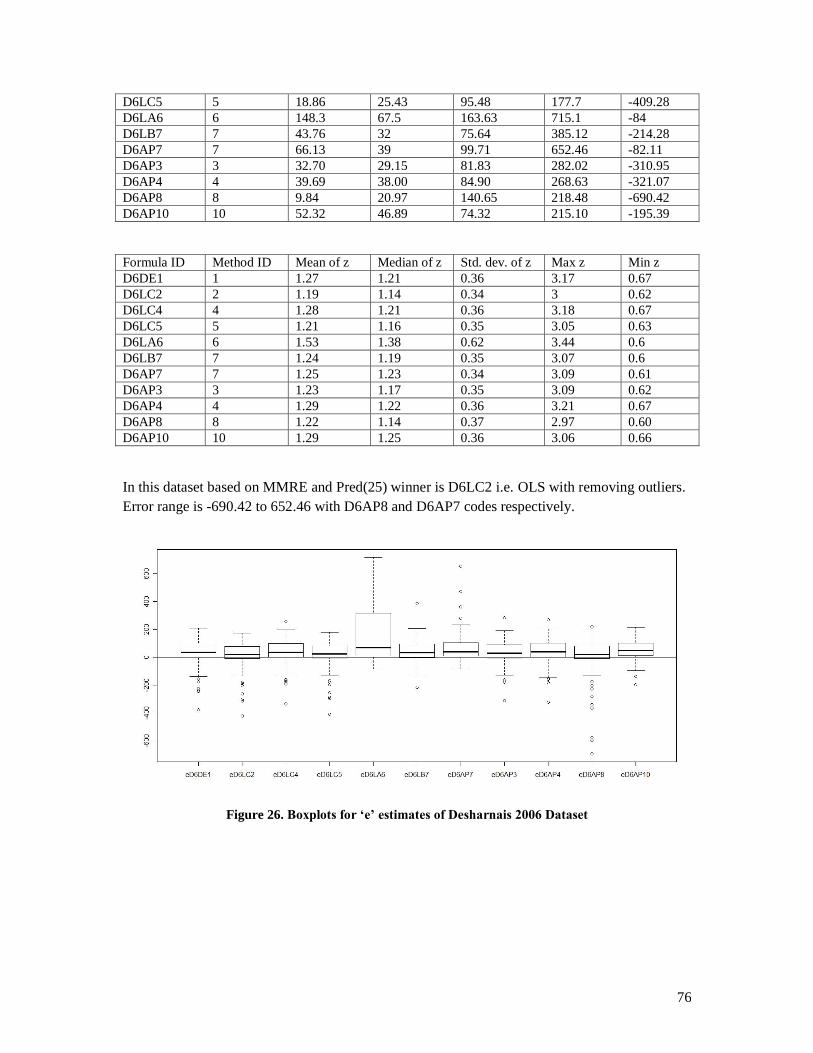
76
D6LC5 5 18.86 25.43 95.48 177.7 -409.28
D6LA6 6 148.3 67.5 163.63 715.1 -84
D6LB7 7 43.76 32 75.64 385.12 -214.28
D6AP7 7 66.13 39 99.71 652.46 -82.11
D6AP3 3 32.70 29.15 81.83 282.02 -310.95
D6AP4 4 39.69 38.00 84.90 268.63 -321.07
D6AP8 8 9.84 20.97 140.65 218.48 -690.42
D6AP10 10 52.32 46.89 74.32 215.10 -195.39
Formula ID Method ID Mean of z Median of z Std. dev. of z Max z Min z
D6DE1 1 1.27 1.21 0.36 3.17 0.67
D6LC2 2 1.19 1.14 0.34 3 0.62
D6LC4 4 1.28 1.21 0.36 3.18 0.67
D6LC5 5 1.21 1.16 0.35 3.05 0.63
D6LA6 6 1.53 1.38 0.62 3.44 0.6
D6LB7 7 1.24 1.19 0.35 3.07 0.6
D6AP7 7 1.25 1.23 0.34 3.09 0.61
D6AP3 3 1.23 1.17 0.35 3.09 0.62
D6AP4 4 1.29 1.22 0.36 3.21 0.67
D6AP8 8 1.22 1.14 0.37 2.97 0.60
D6AP10 10 1.29 1.25 0.36 3.06 0.66
In this dataset based on MMRE and Pred(25) winner is D6LC2 i.e. OLS with removing outliers.
Error range is -690.42 to 652.46 with D6AP8 and D6AP7 codes respectively.
Figure 26. Boxplots for ‘e’ estimates of Desharnais 2006 Dataset
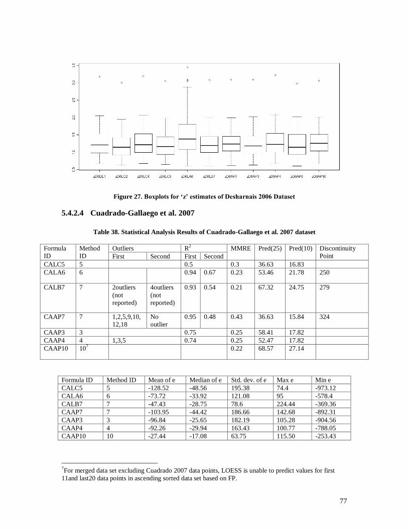
77
Figure 27. Boxplots for ‘z’ estimates of Desharnais 2006 Dataset
5.4.2.4 Cuadrado-Gallaego et al. 2007
Table 38. Statistical Analysis Results of Cuadrado-Gallaego et al. 2007 dataset
Formula
ID
Method
ID
Outliers R2 MMRE Pred(25) Pred(10) Discontinuity
Point First Second First Second
CALC5 5 0.5 0.3 36.63 16.83
CALA6 6 0.94 0.67 0.23 53.46 21.78 250
CALB7 7 2outliers
(not
reported)
4outliers
(not
reported)
0.93 0.54 0.21 67.32 24.75 279
CAAP7 7 1,2,5,9,10,
12,18
No
outlier
0.95 0.48 0.43 36.63 15.84 324
CAAP3 3 0.75 0.25 58.41 17.82
CAAP4 4 1,3,5 0.74 0.25 52.47 17.82
CAAP10 107 0.22 68.57 27.14
Formula ID Method ID Mean of e Median of e Std. dev. of e Max e Min e
CALC5 5 -128.52 -48.56 195.38 74.4 -973.12
CALA6 6 -73.72 -33.92 121.08 95 -578.4
CALB7 7 -47.43 -28.75 78.6 224.44 -369.36
CAAP7 7 -103.95 -44.42 186.66 142.68 -892.31
CAAP3 3 -96.84 -25.65 182.19 105.28 -904.56
CAAP4 4 -92.26 -29.94 163.43 100.77 -788.05
CAAP10 10 -27.44 -17.08 63.75 115.50 -253.43
7For merged data set excluding Cuadrado 2007 data points, LOESS is unable to predict values for first
11and last20 data points in ascending sorted data set based on FP.

78
Formula ID Method ID Mean of z Median of z Std. dev. of z Max z Min z
CALC5 5 0.76 0.69 0.26 1.91 0.41
CALA6 6 0.84 0.78 0.23 2.17 0.45
CALB7 7 0.9 0.83 0.25 1.97 0.48
CAAP7 7 0.68 0.71 0.53 2.76 -1.25
CAAP3 3 0.88 0.81 0.29 2.29 0.45
CAAP4 4 0.85 0.79 0.26 2.24 0.49
CAAP10 10 0.95 0.90 0.29 2.42 0.50
Here winner is CALB7 according to MMRE and Pred(25). Error range is -973.12 to 224.44 for
CALC5 and CALB77 respectively. It is interesting to note that models built with this dataset
tend to underestimate projects rather than overestimating.
Figure 28. Boxplots for ‘e’ estimates of Cuadrado-Gallaego et al. 2007 dataset
Figure 29. Boxplots for ‘z’ estimates of Cuadrado-Gallaego et al. 2007 dataset

79
5.4.2.5 Fetcke 1999 (warehouse portfolio)
Table 39. Statistical Analysis Results of warehouse portfolio dataset
Formula
ID
Method
ID
Outliers R2 MMRE Pred(25) Pred(10) Discontinuity
Point First Second First Second
FEVL1 1 0.99 0.39 44.18 20.93
FEAP3 3 0.98 0.52 29.45 11.62
FEAP4 4 0.98 0.52 29.45 11.62
Formula ID Method ID Mean of e Median of e Std. dev. of e Max e Min e
FEVL1 1 59.63 52.5 81.9 320.4 -270.6
FEAP3 3 117.65 97.48 103.4 661.48 -39.69
FEAP4 4 117.65 97.48 103.4 661.48 -39.69
Formula ID Method ID Mean of z Median of z Std. dev. of z Max z Min z
FEVL1 1 1.36 1.27 0.38 3.45 0.72
FEAP3 3 1.5 1.42 0.41 3.79 0.73
FEAP4 4 1.5 1.42 0.41 3.79 0.73
For this dataset winner is FEVL1 since we don‘t have much data to build different models. Error
range is -270.6 to 661.48 for FEVL1 and FEAP3 respectively. It is interesting to note that
FEAP3 and FEAP4 yield similar results because there is no outlier in dataset. In this dataset it is
not possible to build any piecewise model due to small number of data points i.e. 5 points.
Figure 30. Boxplots for ‘e’ estimates of warehouse portfolio dataset
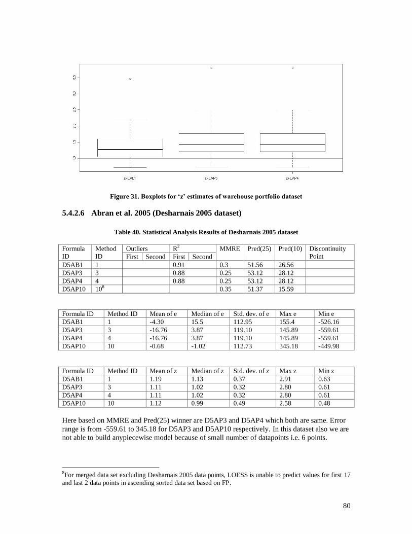
80
Figure 31. Boxplots for ‘z’ estimates of warehouse portfolio dataset
5.4.2.6 Abran et al. 2005 (Desharnais 2005 dataset)
Table 40. Statistical Analysis Results of Desharnais 2005 dataset
Formula
ID
Method
ID
Outliers R2 MMRE Pred(25) Pred(10) Discontinuity
Point First Second First Second
D5AB1 1 0.91 0.3 51.56 26.56
D5AP3 3 0.88 0.25 53.12 28.12
D5AP4 4 0.88 0.25 53.12 28.12
D5AP10 108 0.35 51.37 15.59
Formula ID Method ID Mean of e Median of e Std. dev. of e Max e Min e
D5AB1 1 -4.30 15.5 112.95 155.4 -526.16
D5AP3 3 -16.76 3.87 119.10 145.89 -559.61
D5AP4 4 -16.76 3.87 119.10 145.89 -559.61
D5AP10 10 -0.68 -1.02 112.73 345.18 -449.98
Formula ID Method ID Mean of z Median of z Std. dev. of z Max z Min z
D5AB1 1 1.19 1.13 0.37 2.91 0.63
D5AP3 3 1.11 1.02 0.32 2.80 0.61
D5AP4 4 1.11 1.02 0.32 2.80 0.61
D5AP10 10 1.12 0.99 0.49 2.58 0.48
Here based on MMRE and Pred(25) winner are D5AP3 and D5AP4 which both are same. Error
range is from -559.61 to 345.18 for D5AP3 and D5AP10 respectively. In this dataset also we are
not able to build anypiecewise model because of small number of datapoints i.e. 6 points.
8For merged data set excluding Desharnais 2005 data points, LOESS is unable to predict values for first 17
and last 2 data points in ascending sorted data set based on FP.

81
Figure 32. Boxplots for ‘e’ estimates of Desharnais 2005 dataset
Figure 33. Boxplots for ‘z’ estimates of Desharnais 2005 dataset
5.4.2.7 Cuadrado-Gallaego et al. 2008 (jjcg06)
Table 41. Statistical Analysis Results of jjcg06 dataset
Formula
ID
Method
ID
Outliers R2 MMRE Pred(25) Pred(10) Discontinuity
Point First Second First Second
CBCA1 1 0.7 0.33 40.17 14.52
CBAP3 3 0.81 0.25 50.42 17.09
CBAP4 4 0.81 0.25 50.42 17.09
CBAP6 6 0.66 0.81 0.32 41.02 18.80 346
CBAP10 109 0.33 36.11 11.11
9For merged data set excluding JJCG06 data points, LOESS is unable to predict values for first 19 and last
22 data points in ascending sorted data set based on FP.
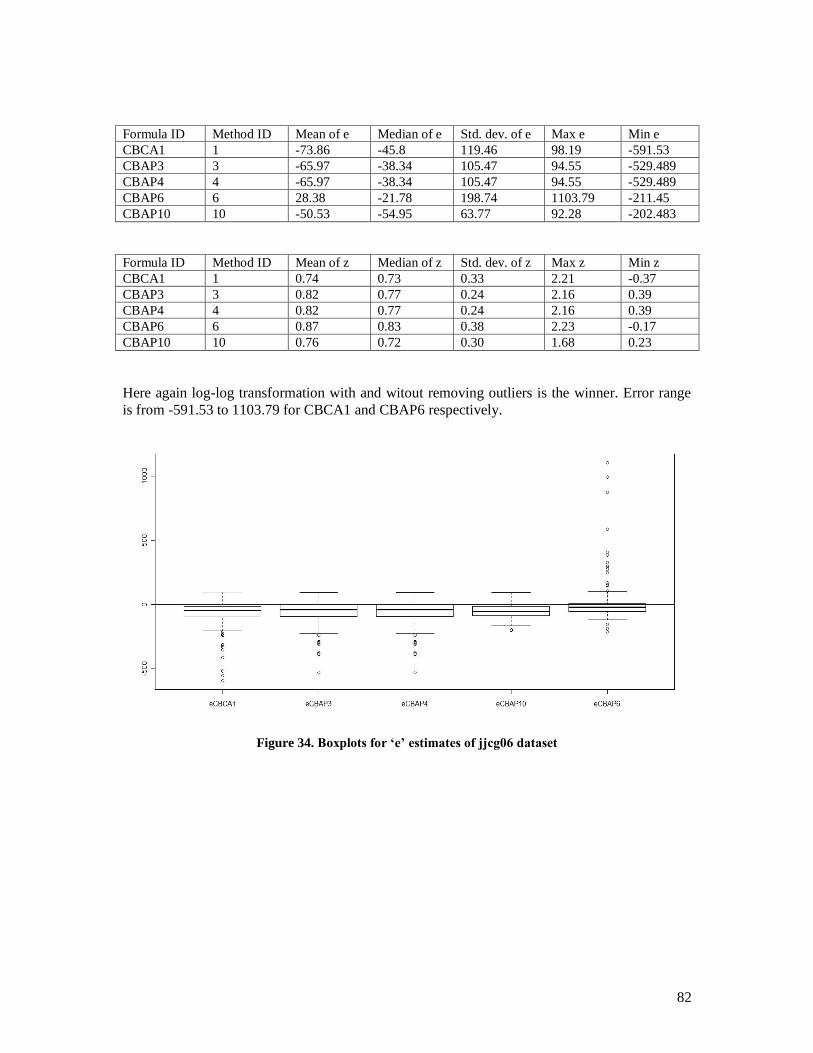
82
Formula ID Method ID Mean of e Median of e Std. dev. of e Max e Min e
CBCA1 1 -73.86 -45.8 119.46 98.19 -591.53
CBAP3 3 -65.97 -38.34 105.47 94.55 -529.489
CBAP4 4 -65.97 -38.34 105.47 94.55 -529.489
CBAP6 6 28.38 -21.78 198.74 1103.79 -211.45
CBAP10 10 -50.53 -54.95 63.77 92.28 -202.483
Formula ID Method ID Mean of z Median of z Std. dev. of z Max z Min z
CBCA1 1 0.74 0.73 0.33 2.21 -0.37
CBAP3 3 0.82 0.77 0.24 2.16 0.39
CBAP4 4 0.82 0.77 0.24 2.16 0.39
CBAP6 6 0.87 0.83 0.38 2.23 -0.17
CBAP10 10 0.76 0.72 0.30 1.68 0.23
Here again log-log transformation with and witout removing outliers is the winner. Error range
is from -591.53 to 1103.79 for CBCA1 and CBAP6 respectively.
Figure 34. Boxplots for ‘e’ estimates of jjcg06 dataset
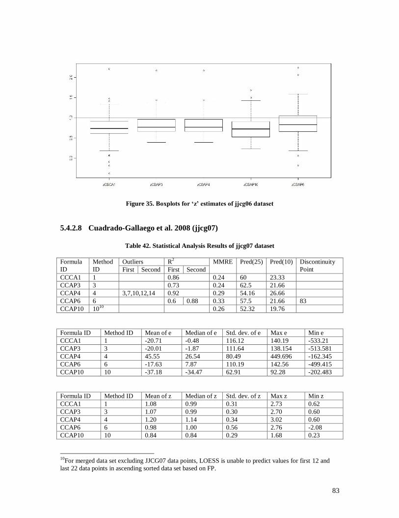
83
Figure 35. Boxplots for ‘z’ estimates of jjcg06 dataset
5.4.2.8 Cuadrado-Gallaego et al. 2008 (jjcg07)
Table 42. Statistical Analysis Results of jjcg07 dataset
Formula
ID
Method
ID
Outliers R2 MMRE Pred(25) Pred(10) Discontinuity
Point First Second First Second
CCCA1 1 0.86 0.24 60 23.33
CCAP3 3 0.73 0.24 62.5 21.66
CCAP4 4 3,7,10,12,14 0.92 0.29 54.16 26.66
CCAP6 6 0.6 0.88 0.33 57.5 21.66 83
CCAP10 1010
0.26 52.32 19.76
Formula ID Method ID Mean of e Median of e Std. dev. of e Max e Min e
CCCA1 1 -20.71 -0.48 116.12 140.19 -533.21
CCAP3 3 -20.01 -1.87 111.64 138.154 -513.581
CCAP4 4 45.55 26.54 80.49 449.696 -162.345
CCAP6 6 -17.63 7.87 110.19 142.56 -499.415
CCAP10 10 -37.18 -34.47 62.91 92.28 -202.483
Formula ID Method ID Mean of z Median of z Std. dev. of z Max z Min z
CCCA1 1 1.08 0.99 0.31 2.73 0.62
CCAP3 3 1.07 0.99 0.30 2.70 0.60
CCAP4 4 1.20 1.14 0.34 3.02 0.60
CCAP6 6 0.98 1.00 0.56 2.76 -2.08
CCAP10 10 0.84 0.84 0.29 1.68 0.23
10
For merged data set excluding JJCG07 data points, LOESS is unable to predict values for first 12 and
last 22 data points in ascending sorted data set based on FP.
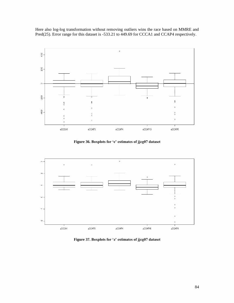
84
Here also log-log transformation without removing outliers wins the race based on MMRE and
Pred(25). Error range for this dataset is -533.21 to 449.69 for CCCA1 and CCAP4 respectively.
Figure 36. Boxplots for ‘e’ estimates of jjcg07 dataset
Figure 37. Boxplots for ‘z’ estimates of jjcg07 dataset
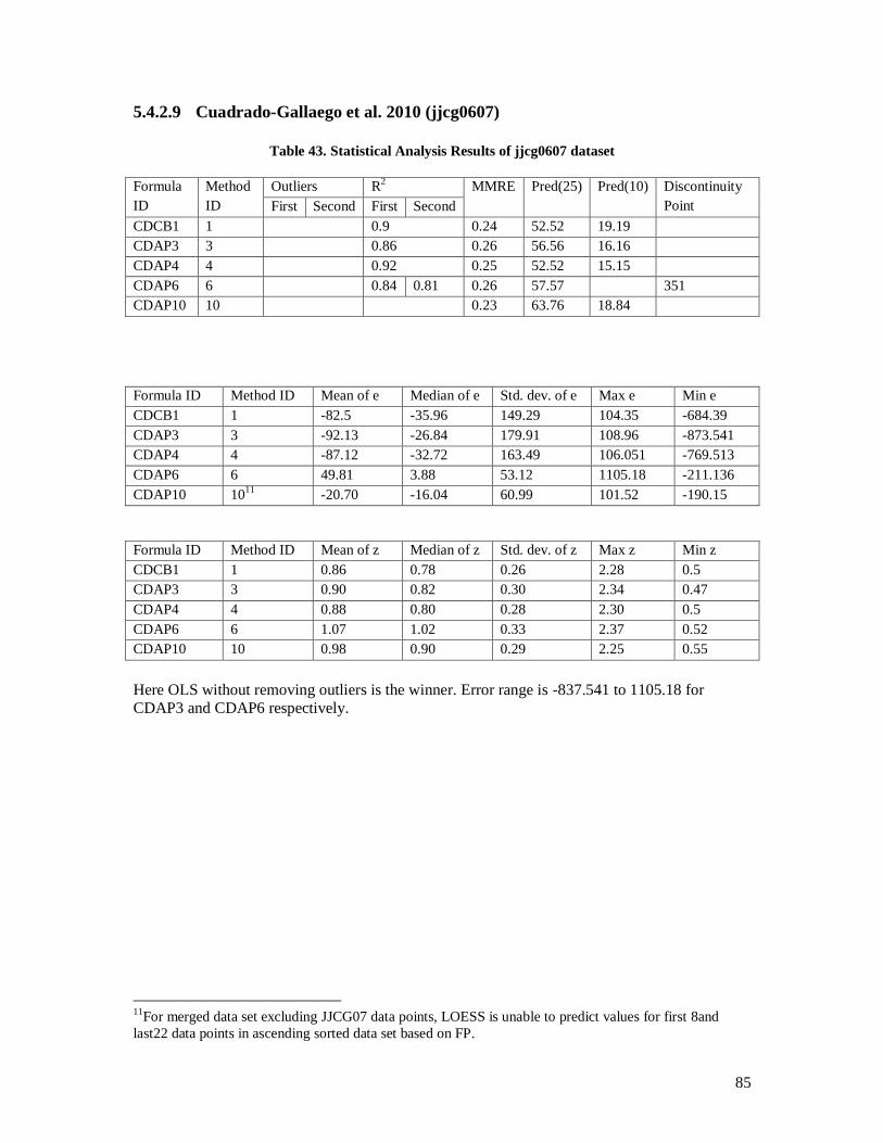
85
5.4.2.9 Cuadrado-Gallaego et al. 2010 (jjcg0607)
Table 43. Statistical Analysis Results of jjcg0607 dataset
Formula
ID
Method
ID
Outliers R2 MMRE Pred(25) Pred(10) Discontinuity
Point First Second First Second
CDCB1 1 0.9 0.24 52.52 19.19
CDAP3 3 0.86 0.26 56.56 16.16
CDAP4 4 0.92 0.25 52.52 15.15
CDAP6 6 0.84 0.81 0.26 57.57 351
CDAP10 10 0.23 63.76 18.84
Formula ID Method ID Mean of e Median of e Std. dev. of e Max e Min e
CDCB1 1 -82.5 -35.96 149.29 104.35 -684.39
CDAP3 3 -92.13 -26.84 179.91 108.96 -873.541
CDAP4 4 -87.12 -32.72 163.49 106.051 -769.513
CDAP6 6 49.81 3.88 53.12 1105.18 -211.136
CDAP10 1011
-20.70 -16.04 60.99 101.52 -190.15
Formula ID Method ID Mean of z Median of z Std. dev. of z Max z Min z
CDCB1 1 0.86 0.78 0.26 2.28 0.5
CDAP3 3 0.90 0.82 0.30 2.34 0.47
CDAP4 4 0.88 0.80 0.28 2.30 0.5
CDAP6 6 1.07 1.02 0.33 2.37 0.52
CDAP10 10 0.98 0.90 0.29 2.25 0.55
Here OLS without removing outliers is the winner. Error range is -837.541 to 1105.18 for
CDAP3 and CDAP6 respectively.
11
For merged data set excluding JJCG07 data points, LOESS is unable to predict values for first 8and
last22 data points in ascending sorted data set based on FP.

86
Figure 38. Boxplots for ‘e’ estimates of jjcg0607 dataset
Figure 39. Boxplots for ‘z’ estimates of jjcg0607 dataset

87
6 A NEW CONVERSION MODEL We developed a new conversion model based on the findings of the SLR. First, we merged all
data from the publicly available datasets and obtained a merged dataset comprising 134 data
points. We used the merged dataset to derive our new conversion model. This merged dataset
can be found in Appendix B, Table-B 15 of this document.
6.1 Relation between IFPUG and COSMIC by Applying
LOESS Before going to make new model first we want to see how FP and CFP behave in different sizes
using merged dataset. We drew scatterplot of merged dataset with a smoothing line generated by
applying LOESS. Figure 40 is the scatter plot of merged dataset.
Figure 40. Merged dataset with a smoothing line using LOESS
By looking at the smoothing line an interesting result can be drawn. The figure shows that data
points follow a piecewise linear regression and the discontinuity point is somewhere between
300 and 400. This finding is in accordance with the systematic approach of finding discontinuity
point. It should be noted that here unlike other authors we didn‘t force data to follow a special
model. For instance we didn‘t plan to model data with linear regression or piecewise linear

88
regression or any other model. Instead of that we applied LOESS regression which doesn‘t force
modeling data to a special model but tries to mimic the real trend between data.
6.2 Approach for Building New Model In order to achieve a new model for conversion between IFPUG and COSMIC we used merged
dataset along with Systematic Approach. We split merged dataset into three parts. Two parts
contain 45 points and one consisted of 44 points. We used one of the 45 points for making the
model, 44 points for optimizing the model and the remaining 45 points for testing model‘s
predictive power. The dataset points for making model, optimizing model and testing model are
shown in Appendix B Table-B 16. By optimizing model we mean finding discontinuity point by
use of MMRE and Pred(25) calculated on part B rather than part A itself. The detailed process of
making model is as follows:
1. Split merged dataset randomly into three parts with 45, 44, and 45 points. Let‘s name
these parts A (model building data), B (training data), and C (test data) respectively.
2. We use part A for making the piecewise model, i.e. we make the first possible model
using 45 points.
3. In this step rather than calculating MMRE and Pred(25) on the same data, we calculate
MMRE and Pred(25) using 44 points i.e. part B and we call these data training data.
4. We make the next model using the part A and again we calculate MMRE and Pred(25)
on part B.
5. We continue mentioned process until all piecewise models using part A are built.
6. We choose the best model based on minimum MMRE and maximum Pred(25).
7. Finally we test our found model using data in part C.
The way we built our model is shown in Figure 41.
The new formula is:
CFP = FP * 0.73 + 3.66 (FP <= 386), R2 = 0.92
CFP = FP * 1.31 - 204.56 (FP > 386), R2 = 0.97
Characteristics for this model by testing on test dataset are: MMRE = 0.19 and pred(25) =
64.44%. This model shows a slight improvement in MMRE compared to models that we have
evaluated. Again there is no statistically significant difference can be found.

89
Figure 41. Pictorial representation of how the model was built
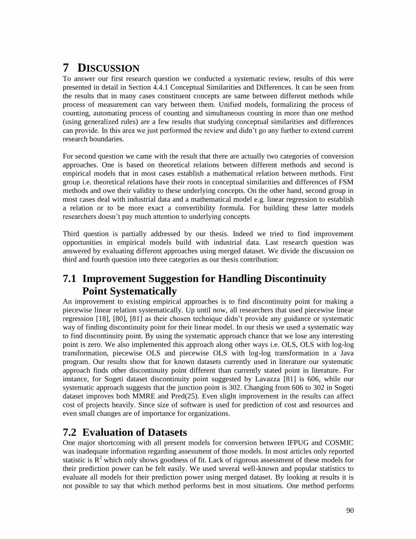
90
7 DISCUSSION To answer our first research question we conducted a systematic review, results of this were
presented in detail in Section 4.4.1 Conceptual Similarities and Differences. It can be seen from
the results that in many cases constituent concepts are same between different methods while
process of measurement can vary between them. Unified models, formalizing the process of
counting, automating process of counting and simultaneous counting in more than one method
(using generalized rules) are a few results that studying conceptual similarities and differences
can provide. In this area we just performed the review and didn‘t go any further to extend current
research boundaries.
For second question we came with the result that there are actually two categories of conversion
approaches. One is based on theoretical relations between different methods and second is
empirical models that in most cases establish a mathematical relation between methods. First
group i.e. theoretical relations have their roots in conceptual similarities and differences of FSM
methods and owe their validity to these underlying concepts. On the other hand, second group in
most cases deal with industrial data and a mathematical model e.g. linear regression to establish
a relation or to be more exact a convertibility formula. For building these latter models
researchers doesn‘t pay much attention to underlying concepts.
Third question is partially addressed by our thesis. Indeed we tried to find improvement
opportunities in empirical models build with industrial data. Last research question was
answered by evaluating different approaches using merged dataset. We divide the discussion on
third and fourth question into three categories as our thesis contribution:
7.1 Improvement Suggestion for Handling Discontinuity
Point Systematically An improvement to existing empirical approaches is to find discontinuity point for making a
piecewise linear relation systematically. Up until now, all researchers that used piecewise linear
regression [18], [80], [81] as their chosen technique didn‘t provide any guidance or systematic
way of finding discontinuity point for their linear model. In our thesis we used a systematic way
to find discontinuity point. By using the systematic approach chance that we lose any interesting
point is zero. We also implemented this approach along other ways i.e. OLS, OLS with log-log
transformation, piecewise OLS and piecewise OLS with log-log transformation in a Java
program. Our results show that for known datasets currently used in literature our systematic
approach finds other discontinuity point different than currently stated point in literature. For
instance, for Sogeti dataset discontinuity point suggested by Lavazza [81] is 606, while our
systematic approach suggests that the junction point is 302. Changing from 606 to 302 in Sogeti
dataset improves both MMRE and Pred(25). Even slight improvement in the results can affect
cost of projects heavily. Since size of software is used for prediction of cost and resources and
even small changes are of importance for organizations.
7.2 Evaluation of Datasets One major shortcoming with all present models for conversion between IFPUG and COSMIC
was inadequate information regarding assessment of those models. In most articles only reported
statistic is R2 which only shows goodness of fit. Lack of rigorous assessment of these models for
their prediction power can be felt easily. We used several well-known and popular statistics to
evaluate all models for their prediction power using merged dataset. By looking at results it is
not possible to say that which method performs best in most situations. One method performs
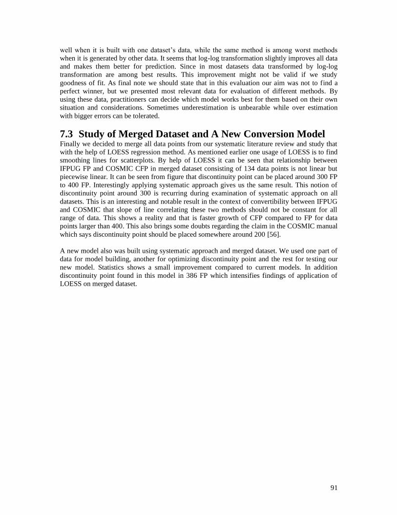
91
well when it is built with one dataset‘s data, while the same method is among worst methods
when it is generated by other data. It seems that log-log transformation slightly improves all data
and makes them better for prediction. Since in most datasets data transformed by log-log
transformation are among best results. This improvement might not be valid if we study
goodness of fit. As final note we should state that in this evaluation our aim was not to find a
perfect winner, but we presented most relevant data for evaluation of different methods. By
using these data, practitioners can decide which model works best for them based on their own
situation and considerations. Sometimes underestimation is unbearable while over estimation
with bigger errors can be tolerated.
7.3 Study of Merged Dataset and A New Conversion Model Finally we decided to merge all data points from our systematic literature review and study that
with the help of LOESS regression method. As mentioned earlier one usage of LOESS is to find
smoothing lines for scatterplots. By help of LOESS it can be seen that relationship between
IFPUG FP and COSMIC CFP in merged dataset consisting of 134 data points is not linear but
piecewise linear. It can be seen from figure that discontinuity point can be placed around 300 FP
to 400 FP. Interestingly applying systematic approach gives us the same result. This notion of
discontinuity point around 300 is recurring during examination of systematic approach on all
datasets. This is an interesting and notable result in the context of convertibility between IFPUG
and COSMIC that slope of line correlating these two methods should not be constant for all
range of data. This shows a reality and that is faster growth of CFP compared to FP for data
points larger than 400. This also brings some doubts regarding the claim in the COSMIC manual
which says discontinuity point should be placed somewhere around 200 [56].
A new model also was built using systematic approach and merged dataset. We used one part of
data for model building, another for optimizing discontinuity point and the rest for testing our
new model. Statistics shows a small improvement compared to current models. In addition
discontinuity point found in this model in 386 FP which intensifies findings of application of
LOESS on merged dataset.
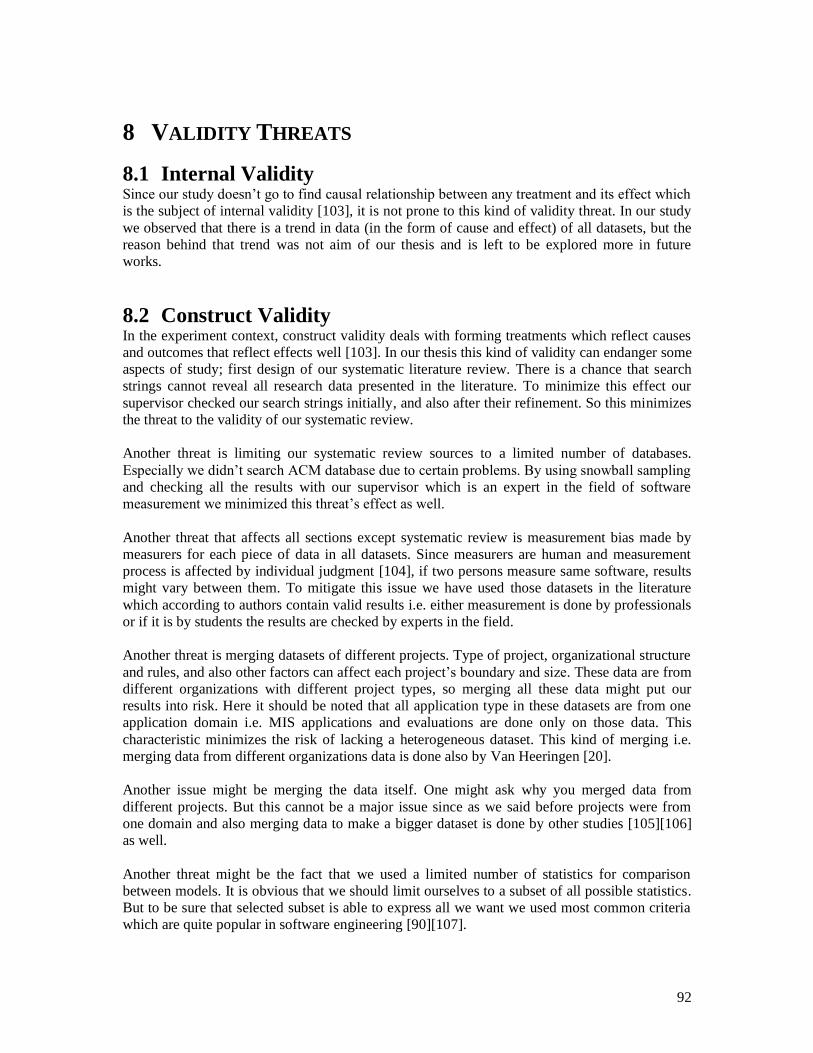
92
8 VALIDITY THREATS
8.1 Internal Validity Since our study doesn‘t go to find causal relationship between any treatment and its effect which
is the subject of internal validity [103], it is not prone to this kind of validity threat. In our study
we observed that there is a trend in data (in the form of cause and effect) of all datasets, but the
reason behind that trend was not aim of our thesis and is left to be explored more in future
works.
8.2 Construct Validity In the experiment context, construct validity deals with forming treatments which reflect causes
and outcomes that reflect effects well [103]. In our thesis this kind of validity can endanger some
aspects of study; first design of our systematic literature review. There is a chance that search
strings cannot reveal all research data presented in the literature. To minimize this effect our
supervisor checked our search strings initially, and also after their refinement. So this minimizes
the threat to the validity of our systematic review.
Another threat is limiting our systematic review sources to a limited number of databases.
Especially we didn‘t search ACM database due to certain problems. By using snowball sampling
and checking all the results with our supervisor which is an expert in the field of software
measurement we minimized this threat‘s effect as well.
Another threat that affects all sections except systematic review is measurement bias made by
measurers for each piece of data in all datasets. Since measurers are human and measurement
process is affected by individual judgment [104], if two persons measure same software, results
might vary between them. To mitigate this issue we have used those datasets in the literature
which according to authors contain valid results i.e. either measurement is done by professionals
or if it is by students the results are checked by experts in the field.
Another threat is merging datasets of different projects. Type of project, organizational structure
and rules, and also other factors can affect each project‘s boundary and size. These data are from
different organizations with different project types, so merging all these data might put our
results into risk. Here it should be noted that all application type in these datasets are from one
application domain i.e. MIS applications and evaluations are done only on those data. This
characteristic minimizes the risk of lacking a heterogeneous dataset. This kind of merging i.e.
merging data from different organizations data is done also by Van Heeringen [20].
Another issue might be merging the data itself. One might ask why you merged data from
different projects. But this cannot be a major issue since as we said before projects were from
one domain and also merging data to make a bigger dataset is done by other studies [105][106]
as well.
Another threat might be the fact that we used a limited number of statistics for comparison
between models. It is obvious that we should limit ourselves to a subset of all possible statistics.
But to be sure that selected subset is able to express all we want we used most common criteria
which are quite popular in software engineering [90][107].
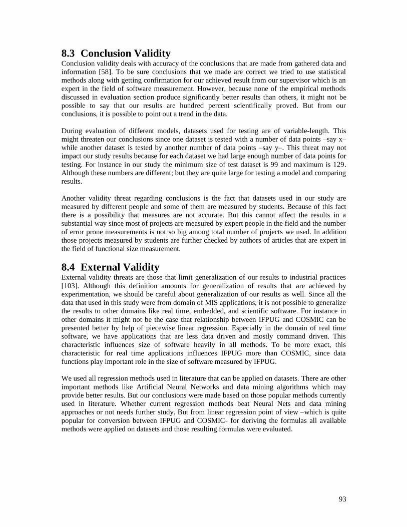
93
8.3 Conclusion Validity Conclusion validity deals with accuracy of the conclusions that are made from gathered data and
information [58]. To be sure conclusions that we made are correct we tried to use statistical
methods along with getting confirmation for our achieved result from our supervisor which is an
expert in the field of software measurement. However, because none of the empirical methods
discussed in evaluation section produce significantly better results than others, it might not be
possible to say that our results are hundred percent scientifically proved. But from our
conclusions, it is possible to point out a trend in the data.
During evaluation of different models, datasets used for testing are of variable-length. This
might threaten our conclusions since one dataset is tested with a number of data points –say x–
while another dataset is tested by another number of data points –say y–. This threat may not
impact our study results because for each dataset we had large enough number of data points for
testing. For instance in our study the minimum size of test dataset is 99 and maximum is 129.
Although these numbers are different; but they are quite large for testing a model and comparing
results.
Another validity threat regarding conclusions is the fact that datasets used in our study are
measured by different people and some of them are measured by students. Because of this fact
there is a possibility that measures are not accurate. But this cannot affect the results in a
substantial way since most of projects are measured by expert people in the field and the number
of error prone measurements is not so big among total number of projects we used. In addition
those projects measured by students are further checked by authors of articles that are expert in
the field of functional size measurement.
8.4 External Validity External validity threats are those that limit generalization of our results to industrial practices
[103]. Although this definition amounts for generalization of results that are achieved by
experimentation, we should be careful about generalization of our results as well. Since all the
data that used in this study were from domain of MIS applications, it is not possible to generalize
the results to other domains like real time, embedded, and scientific software. For instance in
other domains it might not be the case that relationship between IFPUG and COSMIC can be
presented better by help of piecewise linear regression. Especially in the domain of real time
software, we have applications that are less data driven and mostly command driven. This
characteristic influences size of software heavily in all methods. To be more exact, this
characteristic for real time applications influences IFPUG more than COSMIC, since data
functions play important role in the size of software measured by IFPUG.
We used all regression methods used in literature that can be applied on datasets. There are other
important methods like Artificial Neural Networks and data mining algorithms which may
provide better results. But our conclusions were made based on those popular methods currently
used in literature. Whether current regression methods beat Neural Nets and data mining
approaches or not needs further study. But from linear regression point of view –which is quite
popular for conversion between IFPUG and COSMIC- for deriving the formulas all available
methods were applied on datasets and those resulting formulas were evaluated.
94
9 CONCLUSION AND FUTURE WORK
9.1 Conclusion During this thesis, we tried to address issue of conversion between different FSM methods. Four
Research questions were designed and have been answered. In following section we try to
summarize answer to each research question which shows summary of all work done in the
thesis.
In answering RQ1 we concluded that there are common concepts between FSM methods. These
concepts can be used to make conversion easier. Also knowing differences helps us to convert
result of a method to another more easily. This similarities and differences can be used to
propose solutions like Unified model [61], and also helps to make the manual conversion
process [56] easier. We covered this question fully in the results of our systematic review.
To address RQ2 we saw that there are different types of conversion approaches in literature for
FSM methods. Some are based on conceptual similarities and differences between various FSM
methods. Unified model [61] and a formula for conversion from Cuadrado-Gallego [63] are of
this type. Mostly conversion approaches are based on empirical data which lead to statistically-
based formulas. These are also as results of our systematic review in chapter 4.
Answering RQ3 led us to some improvement opportunities. One major improvement
opportunity that was identified in this thesis is to systematically find discontinuity point in
piecewise linear regression. That approach can help practitioners to make better models of their
data. Systematic approach is a general algorithm that selects best model using criteria defined by
the user for assessing model. So, Along with systematic approach practitioners need to decide
how to assess suitability of models. During our thesis we used MMRE and Pred(25) as two well-
known criteria for choosing best models.
Another point that can help for empirical conversion is the fact that relationship between IFPUG
and COSMIC can be presented better if we divide our dataset into two groups, one group for
small applications and another for big applications. This is result of studying merged dataset
with LOESS as a way of applying local regression. It should be noted that applying locally
weighted regressions like LOESS for finding a visual trend is superior to non-locally weighted
regression techniques since we didn‘t force data into a presumed model like piecewise or linear
regression or log-log transformation. To the best of our knowledge no study in the field of
conversion between has used LOESS before. Also no study before this thesis used this amount
of data points in a dataset to find any relationship between COSMIC and IFPUG.
After knowing that nature of relation between IFPUG and COSMIC is piecewise linear, problem
of selecting a point as discontinuity point arises. Different authors in different studies used
various points as discontinuity point. Discontinuity point according to COSMIC manual [28]
was 200. That means projects below 200 should be considered as small and over 200 as large.
Our experience with merged dataset as well as result from study of each dataset shows that
discontinuity point should be somewhere around 300 to 400. This fact might reveal effect of
underlying rules such as boundaries that exist for IFPUG while there is no corresponding
concept in COSMIC. This can be more explored as future work.

95
There are other opportunities in the context of empirical model building like using different
unused model e.g. Artificial Neural Networks and Support Vector Regressions to make more
reliable models for prediction. But these are left as future work.
Finally to answer RQ4, we studied empirical approaches proposed for conversion between
IFPUG and COSMIC and evaluated those based on a merged dataset. That merged dataset is
composed of different publicly available datasets. We evaluated all approaches for their
reliability in prediction of new data. Current articles that address empirical conversion just report
goodness of fit for their approaches. In our study we tested different approaches with unseen and
new data to assess prediction power of the models rather than merely assessing fitness to their
generating data. Our results show that it is not possible to say that one method is significantly
better to predict new data compared to others. We presented statistical results of evaluation
which allows practitioners choose best model based on their own concerns. Some models tend to
overestimate while some others come with under-estimation. This was discussed in chapter 7 of
this work in detail.
9.2 Future Work There are some niches in conversion of FSM methods which can be explored and solution can be
provided. In terms of empirical relation between IFPUG and COSMIC, other models like
Artificial Neural Networks and Support Vector Regressions can be used to make more reliable
models for prediction. Artificial Neural Networks have good reputation in software cost
estimation industry but nobody has used them as a replacement for regression in finding relation
between FSM methods.
Another work that is needed to be done and is directly related to the results of this thesis is
exploring why there is a shift in slope in regression models that represent relation between
IFPUG and COSMIC. As mentioned earlier this slope shift happens somewhere between 300 to
400 FP. Underlying rules and concepts that cause this to happen can be explored which in turn
helps researcher and practitioners make more accurate models considering existence of these
facts.
The next opportunity is to evaluate and test different conceptual models proposed in literature
with new data. Unfortunately mostly researchers provide models but like empirical models they
lack a reliable assessment which leaves practitioners unguided when choosing the appropriate
model.
Another work is to extend implemented application with adding new datasets and building that
application available on the web. Different features like adding new dataset and prediction using
new methods can be added to the application. Using this application many practitioners may add
their own data for making application‘s produced models more reliable.
Finally the new model derived in this thesis needs to be tested with new data. There should be
new projects measured both in COSMIC and IFPUG to test the model found here for its
prediction power and to see how it will behave in that situation.

96
REFERENCES
[1] T. Fetcke, ―A generalized representation for selected Functional size measurement
methods,‖ IN 11TH INTERNATIONAL WORKSHOP ON SOFTWARE MEASUREMENT,
2001.
[2] P. Mohagheghi, B. Anda, and R. Conradi, ―Effort estimation of use cases for incremental
large-scale software development,‖ 2005, pp. 303-311.
[3] B. Boehm, C. Abts, and S. Chulani, ―Software development cost estimation approaches—
A survey,‖ Annals of Software Engineering, vol. 10, no. 1, pp. 177-205, 2000.
[4] B. W. Boehm, R. Madachy, and B. Steece, Software Cost Estimation with Cocomo II.
Prentice Hall PTR Upper Saddle River, NJ, USA, 2000.
[5] L. Lavazza, ―Convertibility of functional size measurements: New insights and
methodological issues,‖ in ACM International Conference Proceeding Series, 2009.
[6] A. J. Albrecht, ―Measuring application development productivity,‖ 1979, vol. 83, p. 92.
[7] A. J. Albrecht and J. E. Gaffney, ―Software Function, Source Lines of Code, and
Development Effort Prediction: A Software Science Validation,‖ Software Engineering,
IEEE Transactions on, vol. 9, no. 6, pp. 639-648, 1983.
[8] J. J. Cuadrado-Gallego, L. Buglione, M. J. Domínguez-Alda, M. F. d. Sevilla, J. Antonio
Gutierrez de Mesa, and O. Demirors, ―An experimental study on the conversion between
IFPUG and COSMIC functional size measurement units,‖ Information and Software
Technology, vol. 52, no. 3, pp. 347-357, 2010.
[9] ―Function Point CPM, Release 4.2.1, Int‘l Function Point Users Group, 2005;
www.ifpug.org.‖
[10] ―ISO/IEC 20968:2002 Software Engineering - MkII Function Point Analysis - Counting
Practices Manual, International Organization for Standardization, ISO,Geneve, 2002.‖
[11] ―ISO/IEC 24570: 2005, Software engineering -- NESMA functional size measurement
method version 2.1 -- Definitions and counting guidelines for the application of Function
Points Analysis, International Organiseation for Standardization -- ISO, Geneva, 2005.‖
[12] ISO/IEC 29881:2008, Software Engineering, FiSMA Functional SizeMeasurement
Method, Version 1.1. International Organization for Standardization, 2008.
[13] ISO/IEC 19761:2003, Software Engineering COSMIC, Software Engineering
COSMIC-Functional Size Measurement Method, International Organization for
Standardization, ISO, Genève, 2003. .
[14] ―ISO/IEC 20926:2003, Software Engineering IFPUG 4.1 Unadjusted FunctionalSize
Measurement Method. Counting Practices Manual, InternationalOrganization for
Standardization, ISO, Genève, 2003.‖ .
[15] G. Rule, ―A comparison of the Mark II and IFPUG variants of Function Point analysis.‖
1999, Available at: http://www.measuresw.com/library/Papers/Rule/MK2IFPUG.html.
[16] J. M. Desharnais, A. Abran, and J. Cuadrado, ―Convertibility of Function Points to
COSMIC-FFP: Identification and Analysis of Functional Outliers,‖ ENSUR A, p. 190,
2006.
[17] C. Gencel and O. Demirors, ―Functional size measurement revisited,‖ ACM Transactions
on Software Engineering and Methodology, vol. 17, no. 3, p. 15 (36 pp.), Jun. 2008.
[18] A. Abran, J. M. Desharnais, and F. Aziz, ―Measurement convertibility-from function
points to COSMIC-FFP,‖ in International Workshop on Software Measurement, 2005.
[19] J. J. Cuadrado-Gallego, D. Rodríguez, F. Machado, and A. Abran, ―Convertibility
between IFPUG and COSMIC functional size measurements,‖ in Lecture Notes in
97
Computer Science (including subseries Lecture Notes in Artificial Intelligence and Lecture
Notes in Bioinformatics), 2007, vol. 4589, pp. 273-283.
[20] H. van Heeringen, ―Changing from FPA to COSMIC-A transition framework,‖ in
Software Measurement European Forum, 2007.
[21] ―ISO/IEC 141431: Information Technology—Software Measurement—Functional Size
Measurement, Part 1: Definition of Concepts, Int‘l Org. for Standardization/ Int‘l
Electrotechnical Commission, 1998.‖
[22] I. ISO, ISO/IEC 14143-2–Information Technology–Software Measurement–Functional
Size Measurement–Part 2: Conformity Evaluation of Software Size Measurement Methods
to ISO. IEC, 2002.
[23] ―ISO ISO/IEC 14143 -3: 2003, Software Engineering- Functional Size Measurement-
Part 3: Verification of Functional Size Measurement Methods, Internat ional Organization
for Standardization - ISO, Geneva, 2003.‖ .
[24] ―ISO/IEC TR 14143-4: Information Technology -- Software Measurement -- Functional
Size Measurement - Part 4: Reference Model, 2002.‖ .
[25] ―ISO/IEC TR 14143-5: Information Technology -- Software Measurement -- Functional
Size Measurement -- Part 5: Determination of Functional Domains for Use with Functional
Size Measurement, 2004.‖ .
[26] ―ISO/IEC FCD 14143-6: Guide for the Use of ISO/IEC 14143 and related International
Standards, 2005.‖ .
[27] D. D. Galorath and M. W. Evans, Software sizing, estimation, and risk management: when
performance is measured performance improves. CRC Press, 2006.
[28] ―The Common Software Measurement Int‘l Consortium FFP, version 3.0, Measurement
Manual, Common Software Measurement Int‘l Consortium, 2007; www.cosmicon.com.‖
[29] S. Oligny, A. Abran, and D. St-Pierre, ―Improving Software Functional Size
Measurement,‖ UQAM Software Engineering Management Research Laboratory, 1999.
[30] A. Abran, ―FFP reléase 2.0: An implementation of COSMIC functional size measurement
concepts,‖ in FESMA, vol. 99, pp. 4–7.
[31] C. R. Symons, ―Function point analysis: difficulties and improvements,‖ Software
Engineering, IEEE Transactions on, vol. 14, no. 1, pp. 2-11, 1988.
[32] C. W. Dawson, Projects on computing and information systems: a student‟s guide.
Pearson Education, 2005.
[33] M. Berndtsson, J. Hansson, B. Olsson, and B. Lundell, Planning and implementing your
final year project--with success!: a guide for students in computer science and information
systems. Springer, 2002.
[34] B. Kitchenham and S. Charters, ―Guidelines for performing systematic literature reviews
in software engineering,‖ Engineering, vol. 2, no. EBSE 2007-001, 2007.
[35] P. Mian, T. Conte, A. Natali, J. Biolchini, and G. Travassos, ―A systematic review process
to software engineering,‖ in Proceedings of the 2nd Experimental Software Engineering
Latin American Workshop (ESELAW‟05), Brazil, 2005.
[36] J. Penrod, D. B. Preston, R. E. Cain, and M. T. Starks, ―A discussion of chain referral as a
method of sampling hard-to-reach populations,‖ Journal of Transcultural Nursing, vol. 14,
no. 2, p. 100, 2003.
[37] J. Faugier and M. Sargeant, ―Sampling hard to reach populations,‖ Journal of Advanced
Nursing, vol. 26, no. 4, pp. 790–797, 1997.
[38] B. Kitchenham and S. Charters, ―Guidelines for performing systematic literature reviews
in software engineering,‖ Engineering, vol. 2, no. EBSE 2007-001, 2007.
[39] K. D. Bailey, Methods of social research. Free Pr, 1994.
[40] H. M. Cooper, L. V. Hedges, and J. C. Valentine, The handbook of research synthesis and
meta-analysis. Russell Sage Foundation, 2009.
98
[41] G. W. Noblit and R. D. Hare, Meta-ethnography: synthesizing qualitative studies. SAGE,
1988.
[42] D. S. Cruzes and T. Dybå, ―Research synthesis in software engineering: A tertiary study,‖
Information and Software Technology, vol. 53, no. 5, pp. 440-455, May 2011.
[43] M. Rodgers et al., ―Testing methodological guidance on the conduct of narrative synthesis
in systematic reviews,‖ Evaluation, vol. 15, no. 1, p. 49, 2009.
[44] M. Dixon-Woods, S. Agarwal, D. Jones, B. Young, and A. Sutton, ―Synthesising
qualitative and quantitative evidence: a review of possible methods,‖ Journal of health
services research & policy, vol. 10, no. 1, p. 45, 2005.
[45] ―Economic & Social Research Council Research MethodsProgramme.
http://www.ccsr.ac.uk/methods/ [accessed 5June 2003].‖ .
[46] K. Walk, ―How to write a comparative Analysis,‖ Writing Center at Harvard University.
Available from http://www. fas. harvard. edu/~ wricntr/documents/CompAnalysis. html.
Internet. Accessed, vol. 5, 2006.
[47] I. Myrtveit and E. Stensrud, ―A controlled experiment to assess the benefits of estimating
with analogy and regression models,‖ IEEE Transactions on Software Engineering, vol.
25, no. 4, pp. 510-525, Aug. 1999.
[48] R Development Core Team, R: A Language and Environment for Statistical Computing.
Vienna, Austria: R Foundation for Statistical Computing.
[49] ―Red-R.‖ [Online]. Available: http://www.red-r.org/.
[50] JGR, http://www.rforge.net/JGR/index.html. .
[51] Deducer, www.deducer.org/manual.html. .
[52] ―Minitab.‖ [Online]. Available: http://www.minitab.com/en-US/default.aspx.
[53] C. Goulding, Grounded theory: a practical guide for management, business and market
researchers. SAGE, 2002.
[54] R. Hoda, J. Noble, and S. Marshall, ―Using grounded theory to study the human aspects of
software engineering,‖ in Human Aspects of Software Engineering on - HAoSE ‟10, Reno,
Nevada, 2010, p. 1.
[55] B. G. Glaser, A. L. Strauss, and E. Strutzel, ―The discovery of grounded theory; strategies
for qualitative research,‖ Nursing Research, vol. 17, no. 4, p. 364, 1968.
[56] ―The COSMIC Functional Size Measurement Method Version 3.0, Advanced and Related
Topics, Common Software Measurement Int‘l Consortium, 2007.‖ .
[57] J. Miller, ―Applying meta-analytical procedures to software engineering experiments,‖
Journal of Systems and Software, vol. 54, no. 1, pp. 29-39, 2000.
[58] J. W. Creswell, Research design: Qualitative, quantitative, and mixed methods
approaches. Sage Publications, Inc, 2009.
[59] J. L. Fleiss, ―Measuring nominal scale agreement among many raters.,‖ Psychological
Bulletin, vol. 76, no. 5, p. 378, 1971.
[60] T. Dyba, T. Dingsoyr, and G. K. Hanssen, ―Applying systematic reviews to diverse study
types: an experience report,‖ in Empirical Software Engineering and Measurement, 2007.
ESEM 2007. First International Symposium on, 2007, pp. 225–234.
[61] C. Ji, S. Yan, X. Ma, and G. Song, ―Unified model of functional size measurement,‖ in
2010 International Conference on E-Product E-Service and E-Entertainment, ICEEE2010,
2010.
[62] P. Efe, C. Gencel, and O. Demirors, ―Mapping Concepts of Functional Size Measurement
Methods,‖ in Cosmic Function Points: Theory and Advanced Practices, CRC Press, 2010.
[63] J. J. Cuadrado-Gallego, F. Machado-Piriz, and J. Aroba-Paez, ―On the conversion between
IFPUG and COSMIC software functional size units: A theoretical and empirical study,‖
Journal of Systems and Software, vol. 81, no. 5, pp. 661-672, 2008.
[64] B. Di Eugenio and M. Glass, ―The kappa statistic: a second look,‖ Computational
Linguistics, vol. 30, pp. 95–101, Mar. 2004.

99
[65] G. Cantone, D. Pace, and G. Calavaro, ―Applying function point to unified modeling
language: conversion model and pilot study,‖ in Software Metrics, 2004. Proceedings. 10th
International Symposium on, 2004, pp. 280-291.
[66] C. J. Lokan, ―An empirical study of the correlations between function point elements
[software metrics],‖ in Software Metrics Symposium, 1999. Proceedings. Sixth
International, 1999, pp. 200-206.
[67] S. Abrahao and E. Insfran, ―A Metamodeling Approach to Estimate Software Size from
Requirements Specifications,‖ in Software Engineering and Advanced Applications, 2008.
SEAA ‟08. 34th Euromicro Conference, 2008, pp. 465-475.
[68] F. Vogelezang and A. Lesterhuis, ―Applicability of COSMIC Full Function Points in an
administrative environment: Experiences of an early adopter,‖ in Proceedings of the 13th
International Workshop on Software Measurement–IWSM 2003, 2003.
[69] T. Fetcke, The warehouse software portfolio: A case study in functional size measurement.
Technische Universit\ät Berlin, Fachbereich 13, Informatik, 1999, Available at:
http://www.fetcke.de/papers/Fetcke1999b.pdf.
[70] V. T. Ho, A. Abran, and T. Fetcke, ―A comparative study case of COSMIC-FFP, full
function point and IFPUG methods,‖ Département d‟informatique, Université du Québec
í?` Montréal, Canada, 1999, Available at:
http://www.gelog.etsmtl.ca/publications/pdf/599.pdf.
[71] C. Symons, ―Conversion between IFPUG 4.0 and MKII Function points,‖ Software
Measurement Services Ltd., Version, vol. 3, 1999.
[72] L. Lavazza, ―A systematic approach to the analysis of function point COSMIC
convertibility,‖ presented at the 20th International Workshop on Software Measurement,
ICSM/Mensura, Stuttgart, 2010.
[73] J. J. Dolado, ―A Study of the relationships among Albrecht and Mark II function points,
lines of code 4GL and effort,‖ Journal of Systems and Software, vol. 37, no. 2, pp. 161-
173, 1997.
[74] T. Kralj, I. Rozman, M. Hericko, and A. Zivkovic, ―Improved standard FPA method -
resolving problems with upper boundaries in the rating complexity process,‖ Journal of
Systems and Software, vol. 77, no. 2, pp. 81-90, 2005.
[75] M. Hericko, I. Rozman, and A. Zivkovic, ―A formal representation of functional size
measurement methods,‖ JOURNAL OF SYSTEMS AND SOFTWARE, vol. 79, no. 9, pp.
1341-1358, Sep. 2006.
[76] C. Gencel and O. Demirors, ―Conceptual Differences Among Functional Size
Measurement Methods,‖ in Empirical Software Engineering and Measurement, 2007.
ESEM 2007. First International Symposium on, 2007, pp. 305-313.
[77] J. Cuadrado-Gallego, L. Buglione, R. Rejas-Muslera, and F. Machado-Piriz, ―IFPUG-
COSMIC Statistical Conversion,‖ PROCEEDINGS OF THE 34TH EUROMICRO
CONFERENCE ON SOFTWARE ENGINEERING, pp. 427-432, 2008.
[78] M. F. Rabbi, S. Natraj, and O. B. Kazeem, ―Evaluation of convertibility issues between
ifpug and cosmic function points,‖ in 4th International Conference on Software
Engineering Advances, ICSEA 2009, Includes SEDES 2009: Simposio para Estudantes de
Doutoramento em Engenharia de Software, 2009, pp. 277-281.
[79] O. Demirors and C. Gencel, ―Conceptual association of functional size measurement
methods,‖ IEEE Software, vol. 26, no. 3, pp. 71-8, May 2009.
[80] L. Lavazza and S. Morasca, ―A study of non-linearity in the statistical convertibility of
function points into cosmic function points,‖ in 24th European Conference on Object-
Oriented Programming, ECOOP 2010 Workshop Proceedings - Workshop 1: Workshop on
Advances in Functional Size Measurement and Effort Estimation, FSM‟10, 2010.
[81] L. Lavazza and S. Morasca, ―Convertibility of Function Points into COSMIC Function
Points: A study using Piecewise Linear Regression,‖ 2011.

100
[82] ―MkII Function Point Analysis Counting Practices Manual v. 1.3.1, Software Metrics
Assoc., 1998; www.uksma.co.uk.‖
[83] A. Abran and P. N. Robillard, ―Function points: a study of their measurement processes
and scale transformations,‖ Journal of Systems and Software, vol. 25, no. 2, pp. 171-184,
1994.
[84] K. Maxwell, Applied statistics for software managers. Prentice Hall PTR, 2002.
[85] B. Kitchenham and E. Mendes, ―Why comparative effort prediction studies may be
invalid,‖ in Proceedings of the 5th International Conference on Predictor Models in
Software Engineering, 2009, p. 4.
[86] S. Morasca, ―Building statistically significant robust regression models in empirical
software engineering,‖ in Proceedings of the 5th International Conference on Predictor
Models in Software Engineering, 2009, p. 19.
[87] P. J. Rousseeuw, A. M. Leroy, and J. Wiley, Robust regression and outlier detection, vol.
3. Wiley Online Library, 1987.
[88] S. S. Shapiro and M. B. Wilk, ―An analysis of variance test for normality (complete
samples),‖ Biometrika, vol. 52, no. 3/4, pp. 591–611, 1965.
[89] R. D. Cook and S. Weisberg, Residuals and influence in regression. Chapman & Hall
New York, 1992.
[90] B. Kitchenham, S. Lawrence Pfleeger, B. McColl, and S. Eagan, ―An empirical study of
maintenance and development estimation accuracy,‖ Journal of systems and software, vol.
64, no. 1, pp. 57–77, 2002.
[91] B. A. Kitchenham, L. M. Pickard, S. G. MacDonell, and M. J. Shepperd, ―What accuracy
statistics really measure [software estimation],‖ in Software, IEE Proceedings-, 2001, vol.
148, pp. 81–85.
[92] T. Foss, E. Stensrud, B. Kitchenham, and I. Myrtveit, ―A simulation study of the model
evaluation criterion MMRE,‖ IEEE Transactions on Software Engineering, pp. 985-995,
2003.
[93] S. Chatterjee and A. S. Hadi, Regression analysis by example. John Wiley and Sons, 2006.
[94] E. Stensrud and I. Myrtveit, ―Human performance estimating with analogy and regression
models: an empirical validation,‖ in Software Metrics Symposium, 1998. Metrics 1998.
Proceedings. Fifth International, 1998, pp. 205–213.
[95] S. Weisberg, Applied linear regression. John Wiley and Sons, 2005.
[96] L. Q. Leal, R. A. . Fagundes, R. M. C. . de Souza, H. P. Moura, and C. M. . Gusmao,
―Nearest-neighborhood linear regression in an application with software effort estimation,‖
in Systems, Man and Cybernetics, 2009. SMC 2009. IEEE International Conference on,
pp. 5030-5034.
[97] P. Kok, B. A. Kitchenham, and J. Kirakowski, ―The MERMAID approach to software
cost estimation,‖ in Esprit Technical Week, 1990.
[98] B. Lo and X. Gao, ―Assessing software cost estimation models: criteria for accuracy,
consistency and regression,‖ Australasian Journal of Information Systems, vol. 5, no. 1,
2007.
[99] B. A. Kitchenham, S. G. MacDonell, L. M. Pickard, and M. J. Shepperd, Assessing
prediction systems. Citeseer, 1999.
[100] S. D. Conte, H. E. Dunsmore, and Y. E. Shen, Software engineering metrics and models.
1986.
[101] R. T. Hughes, A. Cunliffe, and F. Young-Martos, ―Evaluating software development
effort model-building techniques for application in a real-time telecommunications
environment,‖ in Software, IEE Proceedings-, 1998, vol. 145, pp. 29-33.
[102] N. J. Salkind, Encyclopedia of measurement and statistics, 3 vols. SAGE Publications,
Inc, 2007.
101
[103] C. Wohlin, Experimentation in software engineering: an introduction, vol. 6. Springer
Netherlands, 2000.
[104] J. J. Cuadrado-Gallego, L. Buglione, M. F. de Sevilla, P. Rodríguez-Soria, and M. J.
Dominguez, ―Horizontal dispersion of software functional size with IFPUG and COSMIC
units,‖ Advances in Engineering Software, vol. 41, no. 2, pp. 262-269, 2010.
[105] A. Wood, ―Predicting software reliability,‖ Computer, vol. 29, no. 11, pp. 69-77, Nov.
1996.
[106] T. Manoli, N. Gretz, H.-J. Gröne, M. Kenzelmann, R. Eils, and B. Brors, ―Group testing
for pathway analysis improves comparability of different microarray datasets,‖
Bioinformatics, vol. 22, no. 20, pp. 2500 -2506, Oct. 2006.
[107] B. A. Kitchenham, E. Mendes, and G. H. Travassos, ―Cross versus Within-Company Cost
Estimation Studies: A Systematic Review,‖ IEEE Transactions on Software Engineering,
vol. 33, no. 5, pp. 316-329, May 2007.
[108] ―IFPUG: Ifpug: Case study 1 release 3.0. Technical report, International FunctionPoint
Users Group (2005).‖ .
[109] ―IBM: Course registration system. Technical report, IBM Rational (2004).‖ .
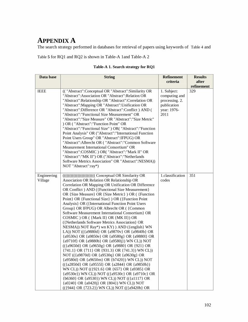
102
APPENDIX A The search strategy performed in databases for retrieval of papers using keywords of Table 4 and
Table 5 for RQ1 and RQ2 is shown in Table-A 1and Table-A 2
Table-A 1. Search strategy for RQ1
Data base String Refinement
criteria
Results
after
refinement
IEEE (( "Abstract":Conceptual OR "Abstract":Similarity OR
"Abstract":Association OR "Abstract":Relation OR
"Abstract":Relationship OR "Abstract":Correlation OR
"Abstract":Mapping OR "Abstract":Unification OR
"Abstract":Difference OR "Abstract":Conflict ) AND (
"Abstract":"Functional Size Measurement" OR
"Abstract":"Size Measure" OR "Abstract":"Size Metric"
) OR ( "Abstract":"Function Point" OR
"Abstract":"Functional Size" ) OR( "Abstract":"Function
Point Analysis" OR ("Abstract":"International Function
Point Users Group" OR "Abstract":IFPUG) OR
"Abstract":Albrecht OR ( "Abstract":"Common Software
Measurement International Consortium" OR
"Abstract":COSMIC ) OR( "Abstract":"Mark II" OR
"Abstract":"MK II") OR ("Abstract":"Netherlands
Software Metrics Association" OR "Abstract":NESMA))
NOT "Abstract":ray*)
1. Subject:
computing and
processing. 2.
publication
year: 1976-
2011
329
Engineering
Village
(((((((((((((((((((((((( Conceptual OR Similarity OR
Association OR Relation OR Relationship OR
Correlation OR Mapping OR Unification OR Difference
OR Conflict ) AND ({Functional Size Measurement}
OR {Size Measure} OR {Size Metric} ) OR ( {Function
Point} OR {Functional Size} ) OR ({Function Point
Analysis} OR ({International Function Point Users
Group} OR IFPUG) OR Albrecht OR ( {Common
Software Measurement International Consortium} OR
COSMIC ) OR ( {Mark II} OR {MK II}) OR
({Netherlands Software Metrics Association} OR
NESMA)) NOT Ray*) wn KY) ) AND ({english} WN
LA)) NOT (({a9880d} OR {a9870v} OR {a9840b} OR
{a9530s} OR {a9850e} OR {a9580g} OR {a9880l} OR
{a9710f} OR {a9880b} OR {a9580j}) WN CL)) NOT
(({a9650d} OR {a9650g} OR {a9880} OR {921} OR
{741.1} OR {711} OR {931.3} OR {741.3}) WN CL))
NOT (({a9870d} OR {a9530q} OR {a9630g} OR
{a9580d} OR {a9650m} OR {b7420}) WN CL)) NOT
(({a2850d} OR {a9555l} OR {a2844} OR {a9850h})
WN CL)) NOT (({921.6} OR {657} OR {a9385} OR
{a9530e}) WN CL)) NOT (({a9530c} OR {a9710c} OR
{b6360} OR {a9530}) WN CL)) NOT (({a1117} OR
{a0240} OR {a0420j} OR {804}) WN CL)) NOT
(({944} OR {723.2}) WN CL)) NOT (({a9420b} OR
1.classification
codes
351
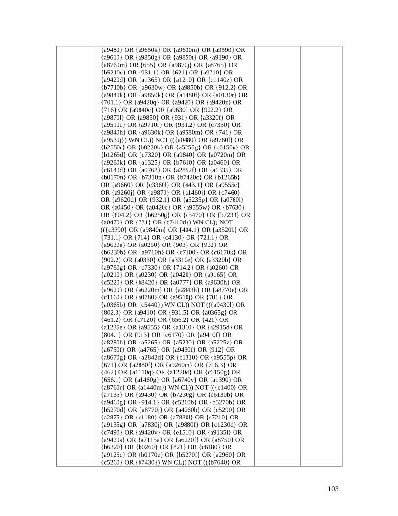
103
{a9480} OR {a9650k} OR {a9630m} OR {a9590} OR
{a9610} OR {a9850g} OR {a9850t} OR {a9190} OR
{a8760m} OR {655} OR {a9870j} OR {a8765} OR
{b5210c} OR {931.1} OR {621} OR {a9710} OR
{a9420d} OR {a1365} OR {a1210} OR {c1140z} OR
{b7710b} OR {a9630w} OR {a9850b} OR {912.2} OR
{a9840k} OR {a9850k} OR {a1480f} OR {a0130r} OR
{701.1} OR {a9420q} OR {a9420} OR {a9420z} OR
{716} OR {a9840c} OR {a9630} OR {922.2} OR
{a9870l} OR {a9850} OR {931} OR {a3320f} OR
{a9510c} OR {a9710r} OR {931.2} OR {c7350} OR
{a9840h} OR {a9630k} OR {a9580m} OR {741} OR
{a9530j}) WN CL)) NOT (({a0480} OR {a9760l} OR
{b2550r} OR {b8220b} OR {a5255g} OR {c6150n} OR
{b1265d} OR {c7320} OR {a9840} OR {a0720m} OR
{a9260k} OR {a1325} OR {b7610} OR {a0460} OR
{c6140d} OR {a0762} OR {a2852f} OR {a1335} OR
{b0170n} OR {b7310n} OR {b7420c} OR {b1265b}
OR {a9660} OR {c3360l} OR {443.1} OR {a9555c}
OR {a9260j} OR {a9870} OR {a1460j} OR {c7460}
OR {a9620d} OR {932.1} OR {a5235p} OR {a0760l}
OR {a0450} OR {a0420c} OR {a9555w} OR {b7630}
OR {804.2} OR {b6250g} OR {c5470} OR {b7230} OR
{a0470} OR {731} OR {c7410d}) WN CL)) NOT
(({c3390} OR {a9840m} OR {404.1} OR {a3520b} OR
{731.1} OR {714} OR {c4130} OR {721.1} OR
{a9630e} OR {a0250} OR {903} OR {932} OR
{b6230b} OR {a9710h} OR {c7100} OR {c6170k} OR
{902.2} OR {a0330} OR {a3310e} OR {a3320b} OR
{a9760g} OR {c7330} OR {714.2} OR {a0260} OR
{a0210} OR {a0230} OR {a0420} OR {a9165} OR
{c5220} OR {b8420} OR {a0777} OR {a9630h} OR
{a9620} OR {a6220m} OR {a2843h} OR {a8770e} OR
{c1160} OR {a0780} OR {a9510j} OR {701} OR
{a0365b} OR {c5440}) WN CL)) NOT (({a9430l} OR
{802.3} OR {a9410} OR {931.5} OR {a0365g} OR
{461.2} OR {c7120} OR {656.2} OR {421} OR
{a1235e} OR {a9555} OR {a1310} OR {a2915d} OR
{804.1} OR {913} OR {c6170} OR {a9410f} OR
{a8280h} OR {a5265} OR {a5230} OR {a5225z} OR
{a6750f} OR {a4765} OR {a9430f} OR {912} OR
{a8670g} OR {a2842d} OR {c1310} OR {a9555p} OR
{671} OR {a2880f} OR {a9260m} OR {716.3} OR
{462} OR {a1110q} OR {a1220d} OR {c6150g} OR
{656.1} OR {a1460g} OR {a6740v} OR {a1390} OR
{a8760r} OR {a1440m}) WN CL)) NOT (({e1400} OR
{a7135} OR {a9430} OR {b7230g} OR {c6130b} OR
{a9460g} OR {914.1} OR {c5260b} OR {b5270b} OR
{b5270d} OR {a8770j} OR {a4260b} OR {c5290} OR
{a2875} OR {c1180} OR {a7830l} OR {c7210} OR
{a9135g} OR {a7830j} OR {a9880f} OR {c1230d} OR
{c7490} OR {a9420v} OR {e1510} OR {a9135l} OR
{a9420s} OR {a7115a} OR {a6220f} OR {a8750} OR
{b6320} OR {b0260} OR {821} OR {c6180} OR
{a9125c} OR {b0170e} OR {b5270f} OR {a2960} OR
{c5260} OR {b7430}) WN CL)) NOT (({b7640} OR
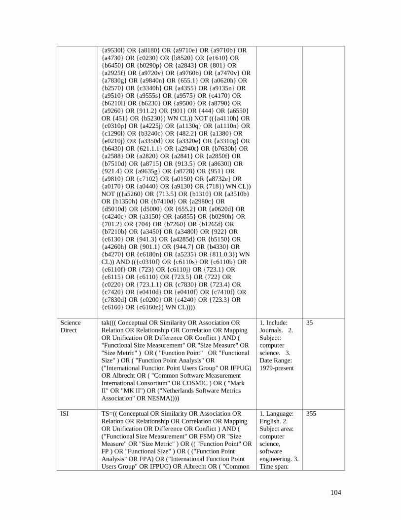
104
{a9530l} OR {a8180} OR {a9710e} OR {a9710b} OR
{a4730} OR {c0230} OR {b8520} OR {e1610} OR
{b6450} OR {b0290p} OR {a2843} OR {801} OR
{a2925f} OR {a9720v} OR {a9760b} OR {a7470v} OR
{a7830g} OR {a9840n} OR {655.1} OR {a0620h} OR
{b2570} OR {c3340h} OR {a4355} OR {a9135n} OR
{a9510} OR {a9555s} OR {a9575} OR {c4170} OR
{b6210l} OR {b6230} OR {a9500} OR {a8790} OR
{a9260} OR {911.2} OR {901} OR {444} OR {a6550}
OR {451} OR {b5230}) WN CL)) NOT (({a4110h} OR
{c0310p} OR {a4225j} OR {a1130q} OR {a1110n} OR
{c1290l} OR {b3240c} OR {482.2} OR {a1380} OR
{e0210j} OR {a3350d} OR {a3320e} OR {a3310g} OR
{b6430} OR {621.1.1} OR {a2940t} OR {b7630b} OR
{a2588} OR {a2820} OR {a2841} OR {a2850f} OR
{b7510d} OR {a8715} OR {913.5} OR {a8630l} OR
{921.4} OR {a9635g} OR {a8728} OR {951} OR
{a9810} OR {c7102} OR {a0150} OR {a8732e} OR
{a0170} OR {a0440} OR {a9130} OR {718}) WN CL))
NOT (({a5260} OR {713.5} OR {b1310} OR {a3510b}
OR {b1350h} OR {b7410d} OR {a2980c} OR
{d5010d} OR {d5000} OR {655.2} OR {a0620d} OR
{c4240c} OR {a3150} OR {a6855} OR {b0290h} OR
{701.2} OR {704} OR {b7260} OR {b1265f} OR
{b7210b} OR {a3450} OR {a3480l} OR {922} OR
{c6130} OR {941.3} OR {a4285d} OR {b5150} OR
{a4260h} OR {901.1} OR {944.7} OR {b4330} OR
{b4270} OR {c6180n} OR {a5235} OR {811.0.3}) WN
CL)) AND (({c0310f} OR {c6110s} OR {c6110b} OR
{c6110f} OR {723} OR {c6110j} OR {723.1} OR
{c6115} OR {c6110} OR {723.5} OR {722} OR
{c0220} OR {723.1.1} OR {c7830} OR {723.4} OR
{c7420} OR {e0410d} OR {e0410f} OR {c7410f} OR
{c7830d} OR {c0200} OR {c4240} OR {723.3} OR
{c6160} OR {c6160z}) WN CL))))
Science
Direct
tak((( Conceptual OR Similarity OR Association OR
Relation OR Relationship OR Correlation OR Mapping
OR Unification OR Difference OR Conflict ) AND (
"Functional Size Measurement" OR "Size Measure" OR
"Size Metric" ) OR ( "Function Point" OR "Functional
Size" ) OR ( "Function Point Analysis" OR
("International Function Point Users Group" OR IFPUG)
OR Albrecht OR ( "Common Software Measurement
International Consortium" OR COSMIC ) OR ( "Mark
II" OR "MK II") OR ("Netherlands Software Metrics
Association" OR NESMA))))
1. Include:
Journals. 2.
Subject:
computer
science. 3.
Date Range:
1979-present
35
ISI TS=(( Conceptual OR Similarity OR Association OR
Relation OR Relationship OR Correlation OR Mapping
OR Unification OR Difference OR Conflict ) AND (
("Functional Size Measurement" OR FSM) OR "Size
Measure" OR "Size Metric" ) OR (( "Function Point" OR
FP ) OR "Functional Size" ) OR ( ("Function Point
Analysis" OR FPA) OR ("International Function Point
Users Group" OR IFPUG) OR Albrecht OR ( "Common
1. Language:
English. 2.
Subject area:
computer
science,
software
engineering. 3.
Time span:
355
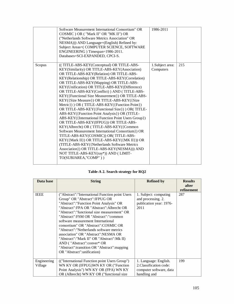
105
Software Measurement International Consortium" OR
COSMIC ) OR ( "Mark II" OR "MK II") OR
("Netherlands Software Metrics Association" OR
NESMA))) AND Language=(English) Refined by:
Subject Areas=( COMPUTER SCIENCE, SOFTWARE
ENGINEERING ) Timespan=1986-2011.
Databases=SCI-EXPANDED, CPCI-S.
1986-2011
Scopus (( TITLE-ABS-KEY(Conceptual) OR TITLE-ABS-
KEY(Similarity) OR TITLE-ABS-KEY(Association)
OR TITLE-ABS-KEY(Relation) OR TITLE-ABS-
KEY(Relationship) OR TITLE-ABS-KEY(Correlation)
OR TITLE-ABS-KEY(Mapping) OR TITLE-ABS-
KEY(Unification) OR TITLE-ABS-KEY(Difference)
OR TITLE-ABS-KEY(Conflict) ) AND ( TITLE-ABS-
KEY({Functional Size Measurement}) OR TITLE-ABS-
KEY({Size Measure}) OR TITLE-ABS-KEY({Size
Metric}) ) OR ( TITLE-ABS-KEY({Function Point})
OR TITLE-ABS-KEY({Functional Size}) ) OR( TITLE-
ABS-KEY({Function Point Analysis}) OR (TITLE-
ABS-KEY({International Function Point Users Group})
OR TITLE-ABS-KEY(IFPUG)) OR TITLE-ABS-
KEY(Albrecht) OR ( TITLE-ABS-KEY({Common
Software Measurement International Consortium}) OR
TITLE-ABS-KEY(COSMIC)) OR( TITLE-ABS-
KEY({Mark II}) OR TITLE-ABS-KEY({MK II})) OR
(TITLE-ABS-KEY({Netherlands Software Metrics
Association}) OR TITLE-ABS-KEY(NESMA))) AND
NOT TITLE-ABS-KEY(ray*)) AND ( LIMIT-
TO(SUBJAREA,"COMP" ) )
1.Subject area:
Computers
215
Table-A 2. Search strategy for RQ2
Data base String Refined by Results
after
refinement
IEEE ("Abstract":"International Function point Users
Group" OR "Abstract":IFPUG OR
"Abstract":"Function Point Analysis" OR
"Abstract":FPA OR "Abstract":Albrecht OR
"Abstract":"functional size measurement" OR
"Abstract":FSM OR "Abstract":"common
software measurement International
consortium" OR "Abstract":COSMIC OR
"Abstract":"Netherlands software metrics
association" OR "Abstract":NESMA OR
"Abstract":"Mark II" OR "Abstract":Mk II)
AND ( "Abstract":conver* OR
"Abstract":transition OR "Abstract":mapping
OR "Abstract":unification)
1. Subject: computing
and processing. 2.
publication year: 1976-
2011
287
Engineering
Village
(("International Function point Users Group")
WN KY OR (IFPUG)WN KY OR ("Function
Point Analysis") WN KY OR (FPA) WN KY
OR (Albrecht) WN KY OR ("functional size
1. Language: English.
2.Classification code:
computer software, data
handling and
199
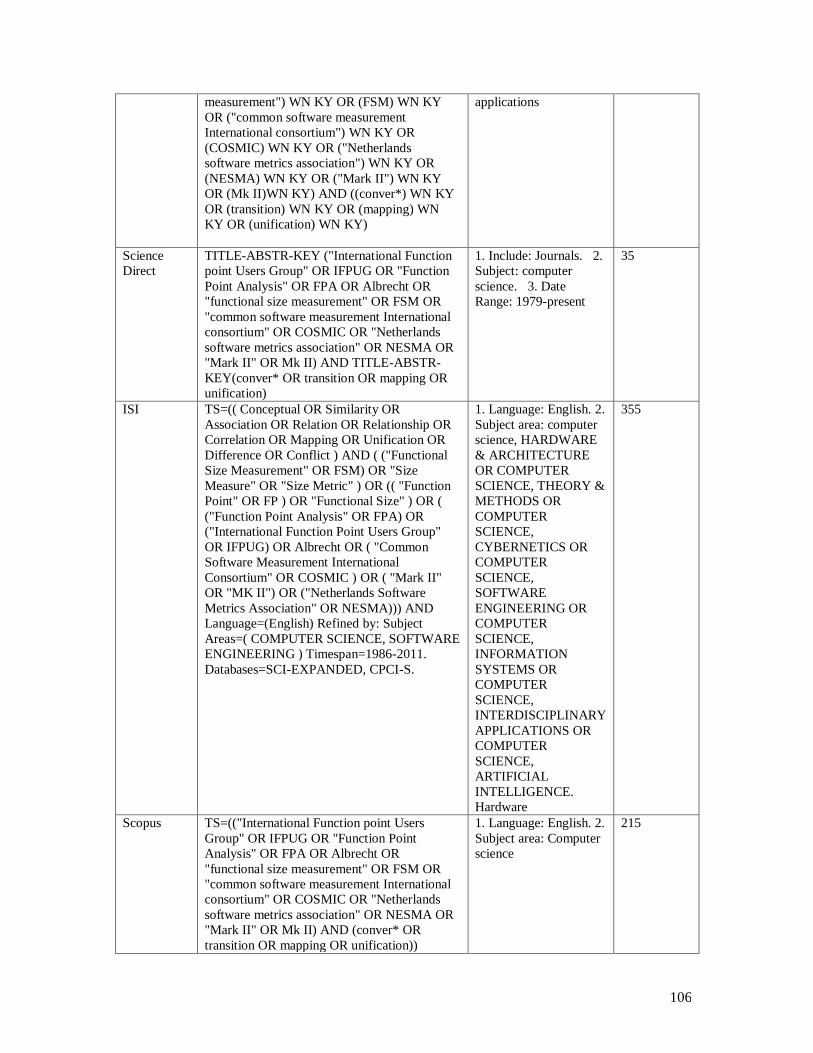
106
measurement") WN KY OR (FSM) WN KY
OR ("common software measurement
International consortium") WN KY OR
(COSMIC) WN KY OR ("Netherlands
software metrics association") WN KY OR
(NESMA) WN KY OR ("Mark II") WN KY
OR (Mk II)WN KY) AND ((conver*) WN KY
OR (transition) WN KY OR (mapping) WN
KY OR (unification) WN KY)
applications
Science
Direct
TITLE-ABSTR-KEY ("International Function
point Users Group" OR IFPUG OR "Function
Point Analysis" OR FPA OR Albrecht OR
"functional size measurement" OR FSM OR
"common software measurement International
consortium" OR COSMIC OR "Netherlands
software metrics association" OR NESMA OR
"Mark II" OR Mk II) AND TITLE-ABSTR-
KEY(conver* OR transition OR mapping OR
unification)
1. Include: Journals. 2.
Subject: computer
science. 3. Date
Range: 1979-present
35
ISI TS=(( Conceptual OR Similarity OR
Association OR Relation OR Relationship OR
Correlation OR Mapping OR Unification OR
Difference OR Conflict ) AND ( ("Functional
Size Measurement" OR FSM) OR "Size
Measure" OR "Size Metric" ) OR (( "Function
Point" OR FP ) OR "Functional Size" ) OR (
("Function Point Analysis" OR FPA) OR
("International Function Point Users Group"
OR IFPUG) OR Albrecht OR ( "Common
Software Measurement International
Consortium" OR COSMIC ) OR ( "Mark II"
OR "MK II") OR ("Netherlands Software
Metrics Association" OR NESMA))) AND
Language=(English) Refined by: Subject
Areas=( COMPUTER SCIENCE, SOFTWARE
ENGINEERING ) Timespan=1986-2011.
Databases=SCI-EXPANDED, CPCI-S.
1. Language: English. 2.
Subject area: computer
science, HARDWARE
& ARCHITECTURE
OR COMPUTER
SCIENCE, THEORY &
METHODS OR
COMPUTER
SCIENCE,
CYBERNETICS OR
COMPUTER
SCIENCE,
SOFTWARE
ENGINEERING OR
COMPUTER
SCIENCE,
INFORMATION
SYSTEMS OR
COMPUTER
SCIENCE,
INTERDISCIPLINARY
APPLICATIONS OR
COMPUTER
SCIENCE,
ARTIFICIAL
INTELLIGENCE.
Hardware
355
Scopus TS=(("International Function point Users
Group" OR IFPUG OR "Function Point
Analysis" OR FPA OR Albrecht OR
"functional size measurement" OR FSM OR
"common software measurement International
consortium" OR COSMIC OR "Netherlands
software metrics association" OR NESMA OR
"Mark II" OR Mk II) AND (conver* OR
transition OR mapping OR unification))
1. Language: English. 2.
Subject area: Computer
science
215

107
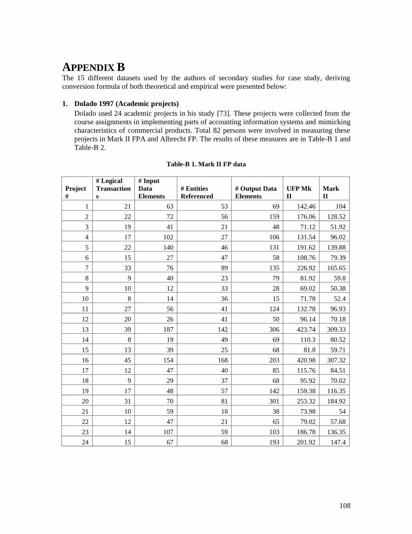
108
APPENDIX B The 15 different datasets used by the authors of secondary studies for case study, deriving
conversion formula of both theoretical and empirical were presented below:
1. Dolado 1997 (Academic projects)
Dolado used 24 academic projects in his study [73]. These projects were collected from the
course assignments in implementing parts of accounting information systems and mimicking
characteristics of commercial products. Total 82 persons were involved in measuring these
projects in Mark II FPA and Albrecht FP. The results of these measures are in Table-B 1 and
Table-B 2.
Table-B 1. Mark II FP data
Project
#
# Logical
Transaction
s
# Input
Data
Elements
# Entities
Referenced
# Output Data
Elements
UFP Mk
II
Mark
II
1 21 63 53 69 142.46 104
2 22 72 56 159 176.06 128.52
3 19 41 21 48 71.12 51.92
4 17 102 27 106 131.54 96.02
5 22 140 46 131 191.62 139.88
6 15 27 47 58 108.76 79.39
7 33 76 89 135 226.92 165.65
8 9 40 23 79 81.92 59.8
9 10 12 33 28 69.02 50.38
10 8 14 36 15 71.78 52.4
11 27 56 41 124 132.78 96.93
12 20 26 41 50 96.14 70.18
13 39 187 142 306 423.74 309.33
14 8 19 49 69 110.3 80.52
15 13 39 25 68 81.8 59.71
16 45 154 168 203 420.98 307.32
17 12 47 40 85 115.76 84.51
18 9 29 37 68 95.92 70.02
19 17 48 57 142 159.38 116.35
20 31 70 81 301 253.32 184.92
21 10 59 18 38 73.98 54
22 12 47 21 65 79.02 57.68
23 14 107 59 103 186.78 136.35
24 15 67 68 193 201.92 147.4
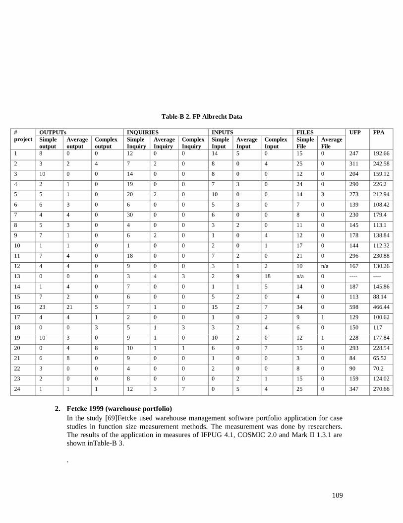
109
Table-B 2. FP Albrecht Data
#
project
OUTPUTs INQUIRIES INPUTS FILES UFP FPA
Simple
output
Average
output
Complex
output
Simple
Inquiry
Average
Inquiry
Complex
Inquiry
Simple
Input
Average
Input
Complex
Input
Simple
File
Average
File
1 8 0 0 12 0 0 14 5 0 15 0 247 192.66
2 3 2 4 7 2 0 8 0 4 25 0 311 242.58
3 10 0 0 14 0 0 8 0 0 12 0 204 159.12
4 2 1 0 19 0 0 7 3 0 24 0 290 226.2
5 5 1 0 20 2 0 10 0 0 14 3 273 212.94
6 6 3 0 6 0 0 5 3 0 7 0 139 108.42
7 4 4 0 30 0 0 6 0 0 8 0 230 179.4
8 5 3 0 4 0 0 3 2 0 11 0 145 113.1
9 7 1 0 6 2 0 1 0 4 12 0 178 138.84
10 1 1 0 1 0 0 2 0 1 17 0 144 112.32
11 7 4 0 18 0 0 7 2 0 21 0 296 230.88
12 4 4 0 9 0 0 3 1 2 10 n/a 167 130.26
13 0 0 0 3 4 3 2 9 18 n/a 0 ---- ----
14 1 4 0 7 0 0 1 1 5 14 0 187 145.86
15 7 2 0 6 0 0 5 2 0 4 0 113 88.14
16 23 21 5 7 1 0 15 2 7 34 0 598 466.44
17 4 4 1 2 0 0 1 0 2 9 1 129 100.62
18 0 0 3 5 1 3 3 2 4 6 0 150 117
19 10 3 0 9 1 0 10 2 0 12 1 228 177.84
20 0 4 8 10 1 1 6 0 7 15 0 293 228.54
21 6 8 0 9 0 0 1 0 0 3 0 84 65.52
22 3 0 0 4 0 0 2 0 0 8 0 90 70.2
23 2 0 0 8 0 0 0 2 1 15 0 159 124.02
24 1 1 1 12 3 7 0 5 4 25 0 347 270.66
2. Fetcke 1999 (warehouse portfolio)
In the study [69]Fetcke used warehouse management software portfolio application for case
studies in function size measurement methods. The measurement was done by researchers.
The results of the application in measures of IFPUG 4.1, COSMIC 2.0 and Mark II 1.3.1 are
shown inTable-B 3.
.

110
Table-B 3. FSM Measures of warehouse management portfolio
Application IFPUG 4.1 COSMIC 2.0 Mark II 1.3.1
Warehouse Portfolio (W) 77 81 72.96
Manufacturers Warehouse (M) 40 38 32.4
Customer Management Application (C) 49 51 46.72
Customer Business Application (LC) 56 52 48.96
Storage Management Application (LS) 31 29 29 24
3. Symons 1999 (Tony Hassan of KPMG Management consulting, London)
Symons [71] used 39 projects in his study for deriving the relation between IFPUG and
Mark II. But dataset details were not available.
4. Vogelezang&Lesterhuis 2003 (Rabobank)
Rabobank is one of the largest banks in Netherlands. Vogelezang & Lesterhuis[68] used
sizing results of Rabobank measures in COSMIC 2.2 and NESMA 2.0 as shown in Table-B
4for deriving possible correlation between them. The measures of NESMA are done by
industry experts and COSMIC is by researchers.
Table-B 4. Rabobank Sizing Results
# Project COSMIC 2.2 NESMA 2.0
1 23 39
2 29 52
3 81 260
4 109 170
5 115 120
6 173 249
7 181 218
8 182 224
9 368 380
10 810 766
11 1662 1424
5. Abran et al 2005 (Desharnais 2005 dataset)
In 2005, Desharnais[18] used dataset from government organization in deriving the relation
between FPA and COSMIC measures. The measures in Table-B 5are measured by researchers
using the documentation of projects. Table-B 5. Desharnais 2005 dataset
Software FPA 4.1 COSMIC 2.2
1 103 75
2 362 209
3 124 170
4 263 203

111
5 1146 934
6 570 675
6. Desharnais et al 2006 (Desharnais 2006 Dataset)
14 MIS projects from single organization were measured by Desharnais in 2006 [16]. The
measurement was done by researchers and detailed results of projects at functional type level
in measures of FPA 4.1 and COSMIC FFP 2.2 are shown inTable-B 6.
Table-B 6. Desharnais 2006 dataset
ID FPA FP 4.1 COSMIC FFP 2.2
Input Output Inquiries ILF & EIF Total FP Entry Exit Read Write Total Cfsu
1 31 145 95 112 383 63 155 120 26 364
2 986 162 168 217 647 96 233 91 45 565
3 104 127 71 98 400 59 125 146 68 398
4 64 55 25 61 205 39 66 55 28 188
5 94 135 66 77 372 52 158 173 65 448
6 22 29 22 53 126 20 37 24 7 88
7 24 21 10 56 111 11 41 47 16 115
8 94 51 72 70 287 45 103 104 46 298
9 202 54 148 96 500 78 110 198 193 579
10 83 128 28 105 344 54 114 92 31 291
11 55 88 69 105 317 49 119 98 28 294
12 103 49 57 49 258 50 86 78 38 252
13 42 35 10 26 113 19 23 39 33 114
14 157 115 70 105 447 67 149 167 84 467
7. Cuadrado-Gallaego et al 2007
Cuadrado-Gallego in 2007 [19]proposed a conversion rule for COSMIC and this was
validated by conducting a case study with 33 projects. Among these 33 projects three are
industrial projects they are: case study documented by IFPUG[108], case study by IBM
rational example RUP[109] and another is the application measured by Fetcke case study
[69]. The remaining 30 are final student projects attending software engineering course at
University of Alcala, Madrid, Spain. The measures in Table-B 7are obtained by three junior
and one senior researcher.
Table-B 7. Projects Measurement Results
Proj ID IFPUG ILF +EIF EI+EO+EQ FTR COSMIC
1 95 5 16 27 68
2 126 10 14 37 80
3 78 3 16 27 72
4 329 25 44 71 177
5 340 14 72 108 195
6 324 6 82 87 267
7 177 9 33 33 108
8 381 12 65 163 278
9 360 12 62 139 210
10 286 14 46 58 191
11 462 14 65 169 286
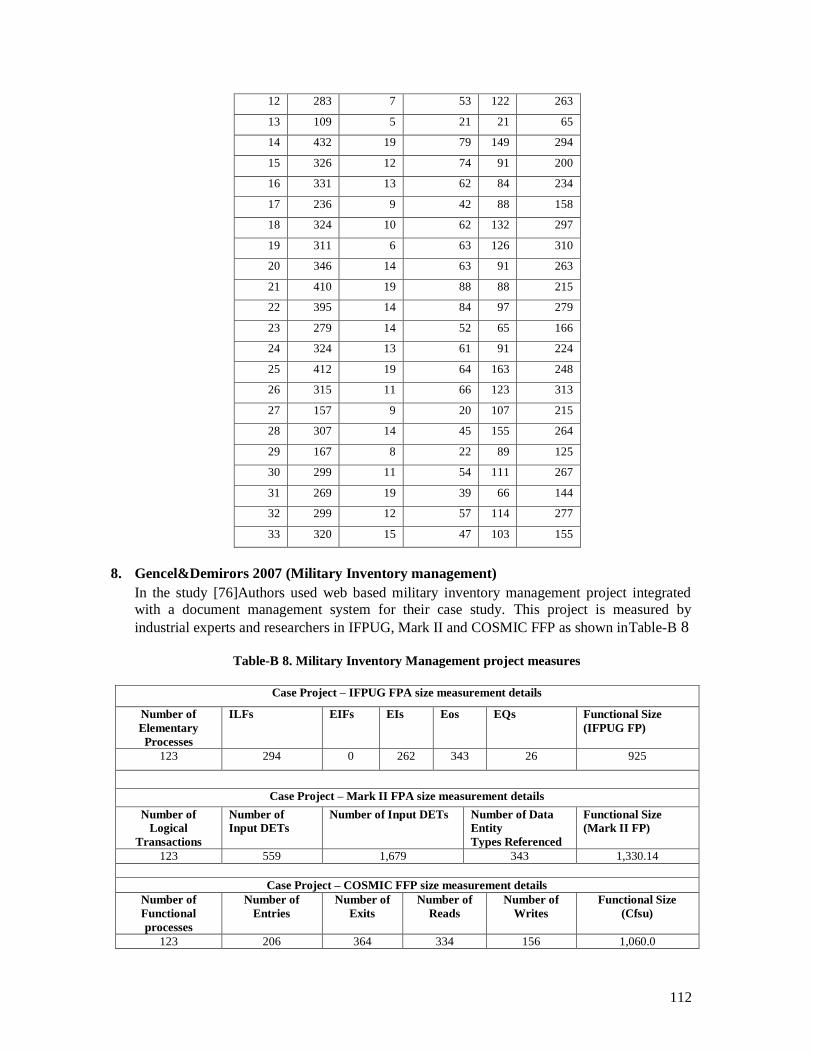
112
12 283 7 53 122 263
13 109 5 21 21 65
14 432 19 79 149 294
15 326 12 74 91 200
16 331 13 62 84 234
17 236 9 42 88 158
18 324 10 62 132 297
19 311 6 63 126 310
20 346 14 63 91 263
21 410 19 88 88 215
22 395 14 84 97 279
23 279 14 52 65 166
24 324 13 61 91 224
25 412 19 64 163 248
26 315 11 66 123 313
27 157 9 20 107 215
28 307 14 45 155 264
29 167 8 22 89 125
30 299 11 54 111 267
31 269 19 39 66 144
32 299 12 57 114 277
33 320 15 47 103 155
8. Gencel&Demirors 2007 (Military Inventory management)
In the study [76]Authors used web based military inventory management project integrated
with a document management system for their case study. This project is measured by
industrial experts and researchers in IFPUG, Mark II and COSMIC FFP as shown inTable-B 8
Table-B 8. Military Inventory Management project measures
Case Project – IFPUG FPA size measurement details
Number of
Elementary
Processes
ILFs EIFs EIs Eos EQs Functional Size
(IFPUG FP)
123 294 0 262 343 26 925
Case Project – Mark II FPA size measurement details
Number of
Logical
Transactions
Number of
Input DETs
Number of Input DETs Number of Data
Entity
Types Referenced
Functional Size
(Mark II FP)
123 559 1,679 343 1,330.14
Case Project – COSMIC FFP size measurement details
Number of
Functional
processes
Number of
Entries
Number of
Exits
Number of
Reads
Number of
Writes
Functional Size
(Cfsu)
123 206 364 334 156 1,060.0
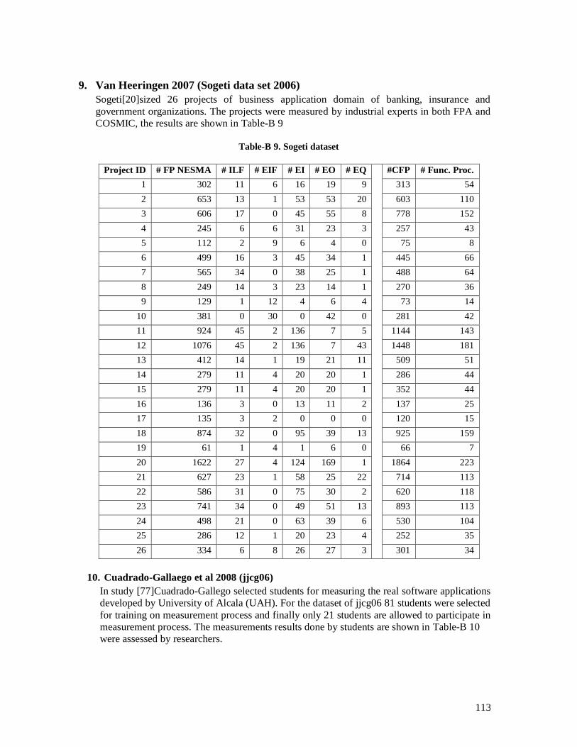
113
9. Van Heeringen 2007 (Sogeti data set 2006)
Sogeti[20]sized 26 projects of business application domain of banking, insurance and
government organizations. The projects were measured by industrial experts in both FPA and
COSMIC, the results are shown in Table-B 9
Table-B 9. Sogeti dataset
Project ID # FP NESMA # ILF # EIF # EI # EO # EQ #CFP # Func. Proc.
1 302 11 6 16 19 9 313 54
2 653 13 1 53 53 20 603 110
3 606 17 0 45 55 8 778 152
4 245 6 6 31 23 3 257 43
5 112 2 9 6 4 0 75 8
6 499 16 3 45 34 1 445 66
7 565 34 0 38 25 1 488 64
8 249 14 3 23 14 1 270 36
9 129 1 12 4 6 4 73 14
10 381 0 30 0 42 0 281 42
11 924 45 2 136 7 5 1144 143
12 1076 45 2 136 7 43 1448 181
13 412 14 1 19 21 11 509 51
14 279 11 4 20 20 1 286 44
15 279 11 4 20 20 1 352 44
16 136 3 0 13 11 2 137 25
17 135 3 2 0 0 0 120 15
18 874 32 0 95 39 13 925 159
19 61 1 4 1 6 0 66 7
20 1622 27 4 124 169 1 1864 223
21 627 23 1 58 25 22 714 113
22 586 31 0 75 30 2 620 118
23 741 34 0 49 51 13 893 113
24 498 21 0 63 39 6 530 104
25 286 12 1 20 23 4 252 35
26 334 6 8 26 27 3 301 34
10. Cuadrado-Gallaego et al 2008 (jjcg06)
In study [77]Cuadrado-Gallego selected students for measuring the real software applications
developed by University of Alcala (UAH). For the dataset of jjcg06 81 students were selected
for training on measurement process and finally only 21 students are allowed to participate in
measurement process. The measurements results done by students are shown in Table-B 10
were assessed by researchers.

114
Table-B 10. jjcg06 Dataset
ID ILF EI EO EQ TI E X W R TC
1 101 141 54 44 340 74 67 45 48 234
2 92 162 66 66 386 49 112 36 72 269
3 98 164 55 43 360 62 86 38 24 210
4 49 72 82 84 284 21 105 16 86 228
5 35 54 20 0 109 21 23 15 6 65
6 131 189 64 54 438 97 79 123 97 396
7 82 114 64 51 311 39 95 38 28 200
8 93 110 58 52 313 75 71 33 55 234
9 63 78 92 42 275 51 60 25 22 158
10 70 111 72 65 318 68 68 23 110 269
11 96 159 91 0 346 73 83 50 43 249
12 98 202 56 39 395 84 70 98 55 307
13 103 96 68 15 282 72 61 41 39 213
14 92 118 81 33 324 70 65 27 62 224
15 123 169 49 27 368 114 70 35 29 248
16 63 25 69 140 397 22 62 110 42 236
17 101 110 90 6 307 43 42 42 137 264
18 84 128 29 64 305 47 61 40 26 174
19 77 86 45 97 305 37 57 33 68 195
20 77 101 82 39 299 72 93 20 82 267
21 133 59 37 41 270 29 29 21 65 144
11. Cuadrado-Gallaego et al 2008 (jjcg07)
This dataset was also from the study. For this dataset measurement process 77 students were
selected for training and only 14 students were selected for measurement process. The
measurement results shown in Table-B 11were reviewed by researchers.
Table-B 11. jjcg07 Dataset
ID ILF EI EO EQ TI E X W R TC
1 103 141 48 59 351 75 58 66 102 301
2 21 24 12 9 66 11 13 8 14 46
3 42 29 23 0 94 20 26 10 11 67
4 42 32 20 12 106 16 38 8 11 54
5 49 48 23 21 134 25 14 13 29 81
6 47 27 48 11 133 41 30 34 6 111
7 28 67 28 18 137 33 33 18 33 117
8 34 12 4 21 71 2 25 1 24 52
9 28 39 8 6 81 32 41 12 30 115
10 42 64 4 44 154 32 55 15 23 125

115
11 42 54 18 12 126 38 23 19 34 114
12 49 42 36 12 139 56 60 16 36 168
13 35 36 12 0 83 20 25 17 12 74
14 42 29 23 0 94 21 24 14 33 92
12. Cuadrado-Gallaego et al 2010 (jjcg0607)
It is the combined data set of jjcg06 and jjcg07 with 35 Projects (21+14) used in study [8].
13. Rabbi et al 2009 (simple locator)
This is a Case study used in[78].This project is measured by researchers and measurement
results are shown inTable-B 12.
Table-B 12. Simple Locator dataset
IFPUG FP COSMIC FFP
46 25
14. Rabbi et al 2009 (PCGEEK)
Case study used in[78] is a company process description project. This project is measured by
researchers. Table-B 13shows the results.
Table-B 13. PCGeek dataset
IFPUG FP COSMIC FFP
154 97
15. Gencel & Demirors 2009 (Avionics management system)
This dataset is used as second case study in [79] by authors. The two sub projects involved
are small to medium commercial aircraft on flight display system. These sub projects are
measured by researchers. Table-B 14 shows the measures of Avionics management system.
Table-B 14. Avionics Management system dataset
Case Project – IFPUG FPA size measurement details
Number of
Elementary
Processes
Number
of
Internal
Logical
Files
(ILFs)
Number
of
External
Interface
Files EIFs
Number
of
External
Inputs
Number
of
External
Outputs
Number
of
External
Inquiries
Functional
Size
(IFPUG
FP)
Project 2a NA NA NA NA NA NA NA
Project 2b 172 38 21 123 14 35 1091.0
Case Project – Mark II FPA size measurement details
Number of
Logical
Transactions
Number
of Input
Data
Element
Types
(DETs)
Number of Input Data
Element Types (DETs
)
Number of Data
Entity
Types Referenced
Functional
Size (Mark
II FP)
Project 2a 33 112 160 198 435.24
Project 2b 172 225 569 633 1329.22

116
Case Project – Mark II FPA size measurement details
Number of
Functional processes
Number
of
Entries
Number of
Exits
Number of
Reads
Number
of Writes
Functional
Size (Cfsu)
Project 2a 33 49 32 198 0 279.0
Project 2b 172 225 258 566 172 1221.0
16. Merged Dataset
Table-B 15 shows merged dataset sorted based on IFPUG FP along their corresponding original
dataset. Table-B 15. Merged Dataset
FP CFP Dataset FP CFP Dataset FP CFP Dataset FP CFP Dataset 31 29 Fetcke 137 117 Cuadrado jj07 305 174 Cuadrado jj06 386 269 Cuadrado jj06
39 23 Rabbobank 139 168 Cuadrado jj07 305 195 Cuadrado jj06 395 307 Cuadrado jj06
40 38 Fetcke 154 125 Cuadrado jj07 307 264 Cuadrado jj06 395 279 Cuadrado 2007
46 25 Rabbi 154 97 Rabbi 307 264 Cuadrado 2007 397 236 Cuadrado jj06
49 51 Fetcke 157 215 Cuadrado 2007 311 200 Cuadrado jj06 400 398 Desharnais 2006
52 29 Rabbobank 167 125 Cuadrado 2007 311 310 Cuadrado 2007 410 215 Cuadrado 2007
56 52 Fetcke 170 109 Rabbobank 313 234 Cuadrado jj06 412 509 Sogeti
61 66 Sogeti 177 108 Cuadrado 2007 315 313 Cuadrado 2007 412 248 Cuadrado 2007
66 46 Cuadrado jj07 205 188 Desharnais 2006 317 294 Desharnais 2006 432 294 Cuadrado 2007
71 52 Cuadrado jj07 218 181 Rabbobank 318 269 Cuadrado jj06 438 396 Cuadrado jj06
77 81 Fetcke 224 182 Rabbobank 320 155 Cuadrado 2007 447 467 Desharnais 2006
78 72 Cuadrado 2007 236 158 Cuadrado 2007 324 224 Cuadrado jj06 462 286 Cuadrado 2007
81 115 Cuadrado jj07 245 257 Sogeti 324 267 Cuadrado 2007 498 530 Sogeti
83 74 Cuadrado jj07 249 270 Sogeti 324 297 Cuadrado 2007 499 445 Sogeti
94 67 Cuadrado jj07 249 173 Rabbobank 324 224 Cuadrado 2007 500 579 Desharnais 2006
94 92 Cuadrado jj07 258 252 Desharnais 2006 326 200 Cuadrado 2007 565 488 Sogeti
95 68 Cuadrado 2007 260 81 Rabbobank 329 177 Cuadrado 2007 570 675 Desharnais 2005
103 75 Desharnais 2005 263 203 Desharnais 2005 331 234 Cuadrado 2007 586 620 Sogeti
106 54 Cuadrado jj07 269 144 Cuadrado 2007 334 301 Sogeti 606 778 Sogeti
109 65 Cuadrado jj06 270 144 Cuadrado jj06 340 234 Cuadrado jj06 627 714 Sogeti
109 65 Cuadrado 2007 275 158 Cuadrado jj06 340 195 Cuadrado 2007 647 565 Desharnais 2006
111 115 Desharnais 2006 279 286 Sogeti 344 291 Desharnais 2006 653 603 Sogeti
112 75 Sogeti 279 352 Sogeti 346 249 Cuadrado jj06 741 893 Sogeti
113 114 Desharnais 2006 279 166 Cuadrado 2007 346 263 Cuadrado 2007 766 810 Rabbobank
120 115 Rabbobank 282 213 Cuadrado jj06 351 301 Cuadrado jj07 874 925 Sogeti
124 170 Desharnais 2005 283 263 Cuadrado 2007 360 210 Cuadrado jj06 924 1144 Sogeti
126 88 Desharnais 2006 284 228 Cuadrado jj06 360 210 Cuadrado 2007 925 1060 Gencel 2007
126 114 Cuadrado jj07 286 252 Sogeti 362 209 Desharnais 2005 1076 1448 Sogeti
126 80 Cuadrado 2007 286 191 Cuadrado 2007 368 248 Cuadrado jj06 1091 1221 Demirors 2009
129 73 Sogeti 287 298 Desharnais 2006 372 448 Desharnais 2006 1146 934 Desharnais 2005
133 111 Cuadrado jj07 299 267 Cuadrado jj06 380 368 Rabbobank 1424 1662 Rabbobank
134 81 Cuadrado jj07 299 267 Cuadrado 2007 381 281 Sogeti 1622 1864 Sogeti
135 120 Sogeti 299 277 Cuadrado 2007 381 278 Cuadrado 2007 136 137 Sogeti 302 313 Sogeti 383 364 Desharnais 2006
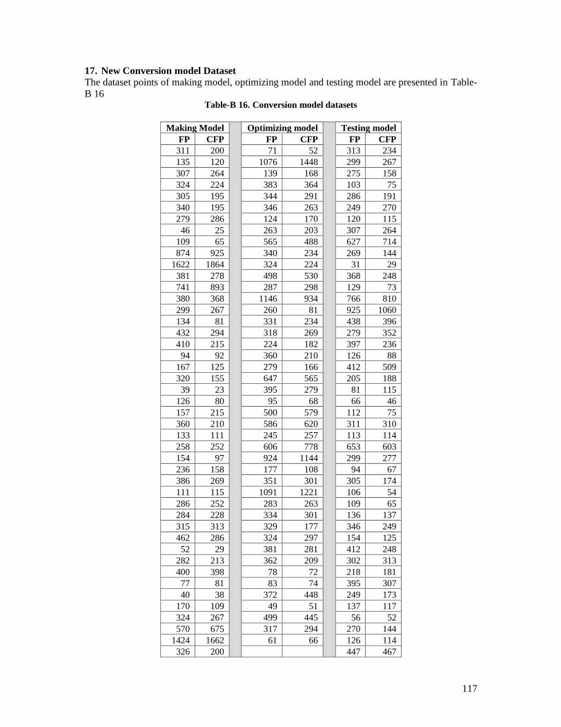
117
17. New Conversion model Dataset
The dataset points of making model, optimizing model and testing model are presented in Table-
B 16 Table-B 16. Conversion model datasets
Making Model
Optimizing model
Testing model
FP CFP FP CFP FP CFP
311 200 71 52 313 234
135 120 1076 1448 299 267
307 264 139 168 275 158
324 224 383 364 103 75
305 195 344 291 286 191
340 195 346 263 249 270
279 286 124 170 120 115
46 25 263 203 307 264
109 65 565 488 627 714
874 925 340 234 269 144
1622 1864 324 224 31 29
381 278 498 530 368 248
741 893 287 298 129 73
380 368 1146 934 766 810
299 267 260 81 925 1060
134 81 331 234 438 396
432 294 318 269 279 352
410 215 224 182 397 236
94 92 360 210 126 88
167 125 279 166 412 509
320 155 647 565 205 188
39 23 395 279 81 115
126 80 95 68 66 46
157 215 500 579 112 75
360 210 586 620 311 310
133 111 245 257 113 114
258 252 606 778 653 603
154 97 924 1144 299 277
236 158 177 108 94 67
386 269 351 301 305 174
111 115 1091 1221 106 54
286 252 283 263 109 65
284 228 334 301 136 137
315 313 329 177 346 249
462 286 324 297 154 125
52 29 381 281 412 248
282 213 362 209 302 313
400 398 78 72 218 181
77 81 83 74 395 307
40 38 372 448 249 173
170 109 49 51 137 117
324 267 499 445 56 52
570 675 317 294 270 144
1424 1662 61 66 126 114
326 200 447 467
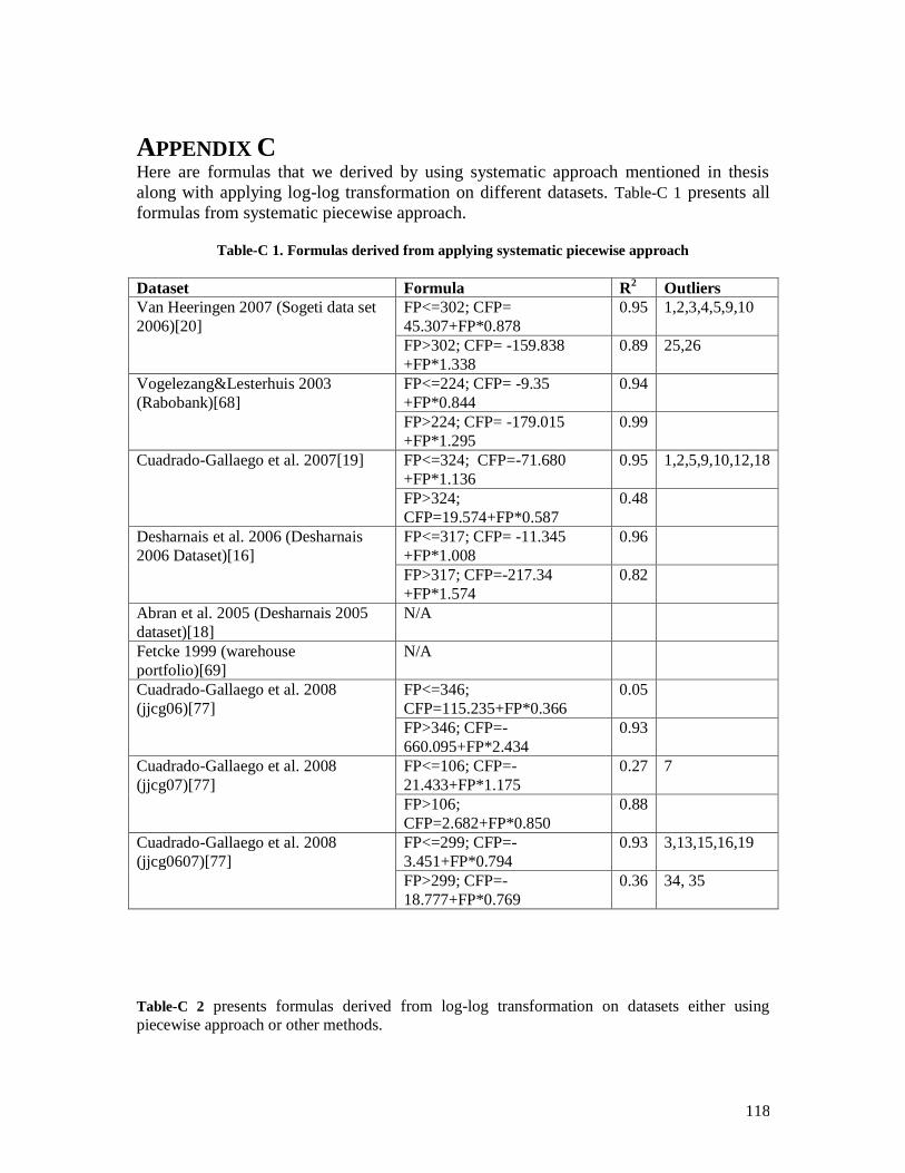
118
APPENDIX C Here are formulas that we derived by using systematic approach mentioned in thesis
along with applying log-log transformation on different datasets. Table-C 1 presents all
formulas from systematic piecewise approach.
Table-C 1. Formulas derived from applying systematic piecewise approach
Dataset Formula R2
Outliers
Van Heeringen 2007 (Sogeti data set
2006)[20]
FP<=302; CFP=
45.307+FP*0.878
0.95 1,2,3,4,5,9,10
FP>302; CFP= -159.838
+FP*1.338
0.89 25,26
Vogelezang&Lesterhuis 2003
(Rabobank)[68]
FP<=224; CFP= -9.35
+FP*0.844
0.94
FP>224; CFP= -179.015
+FP*1.295
0.99
Cuadrado-Gallaego et al. 2007[19] FP<=324; CFP=-71.680
+FP*1.136
0.95 1,2,5,9,10,12,18
FP>324;
CFP=19.574+FP*0.587
0.48
Desharnais et al. 2006 (Desharnais
2006 Dataset)[16]
FP<=317; CFP= -11.345
+FP*1.008
0.96
FP>317; CFP=-217.34
+FP*1.574
0.82
Abran et al. 2005 (Desharnais 2005
dataset)[18]
N/A
Fetcke 1999 (warehouse
portfolio)[69]
N/A
Cuadrado-Gallaego et al. 2008
(jjcg06)[77]
FP<=346;
CFP=115.235+FP*0.366
0.05
FP>346; CFP=-
660.095+FP*2.434
0.93
Cuadrado-Gallaego et al. 2008
(jjcg07)[77]
FP<=106; CFP=-
21.433+FP*1.175
0.27 7
FP>106;
CFP=2.682+FP*0.850
0.88
Cuadrado-Gallaego et al. 2008
(jjcg0607)[77]
FP<=299; CFP=-
3.451+FP*0.794
0.93 3,13,15,16,19
FP>299; CFP=-
18.777+FP*0.769
0.36 34, 35
Table-C 2 presents formulas derived from log-log transformation on datasets either using
piecewise approach or other methods.
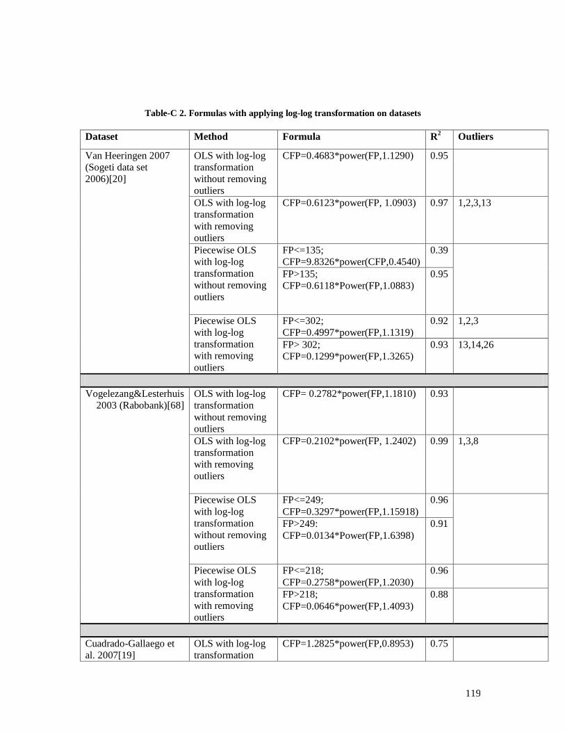
119
Table-C 2. Formulas with applying log-log transformation on datasets
Dataset Method Formula R2
Outliers
Van Heeringen 2007
(Sogeti data set
2006)[20]
OLS with log-log
transformation
without removing
outliers
CFP=0.4683*power(FP,1.1290) 0.95
OLS with log-log
transformation
with removing
outliers
CFP=0.6123*power(FP, 1.0903) 0.97 1,2,3,13
Piecewise OLS
with log-log
transformation
without removing
outliers
FP<=135;
CFP=9.8326*power(CFP,0.4540)
0.39
FP>135;
CFP=0.6118*Power(FP,1.0883)
0.95
Piecewise OLS
with log-log
transformation
with removing
outliers
FP<=302;
CFP=0.4997*power(FP,1.1319)
0.92 1,2,3
FP> 302;
CFP=0.1299*power(FP,1.3265)
0.93 13,14,26
Vogelezang&Lesterhuis
2003 (Rabobank)[68]
OLS with log-log
transformation
without removing
outliers
CFP= 0.2782*power(FP,1.1810) 0.93
OLS with log-log
transformation
with removing
outliers
CFP=0.2102*power(FP, 1.2402) 0.99 1,3,8
Piecewise OLS
with log-log
transformation
without removing
outliers
FP<=249;
CFP=0.3297*power(FP,1.15918)
0.96
FP>249:
CFP=0.0134*Power(FP,1.6398)
0.91
Piecewise OLS
with log-log
transformation
with removing
outliers
FP<=218;
CFP=0.2758*power(FP,1.2030)
0.96
FP>218;
CFP=0.0646*power(FP,1.4093)
0.88
Cuadrado-Gallaego et
al. 2007[19]
OLS with log-log
transformation
CFP=1.2825*power(FP,0.8953) 0.75
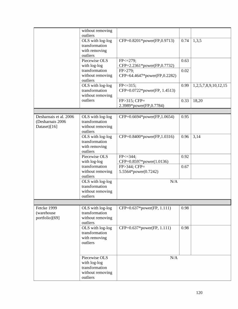
120
without removing
outliers
OLS with log-log
transformation
with removing
outliers
CFP=0.8201*power(FP,0.9713) 0.74 1,3,5
Piecewise OLS
with log-log
transformation
without removing
outliers
FP<=279;
CFP=2.2361*power(FP,0.7732)
0.63
FP>279;
CFP=64.4647*power(FP,0.2282)
0.02
OLS with log-log
transformation
without removing
outliers
FP<=315;
CFP=0.0722*power(FP, 1.4513)
0.99 1,2,5,7,8,9,10,12,15
FP>315; CFP=
2.3989*power(FP,0.7784)
0.33 18,20
Desharnais et al. 2006
(Desharnais 2006
Dataset)[16]
OLS with log-log
transformation
without removing
outliers
CFP=0.6694*power(FP,1.0654) 0.95
OLS with log-log
transformation
with removing
outliers
CFP=0.8400*power(FP,1.0316) 0.96 3,14
Piecewise OLS
with log-log
transformation
without removing
outliers
FP<=344;
CFP=0.8597*power(1.0136)
0.92
FP>344; CFP=
5.5564*power(0.7242)
0.67
OLS with log-log
transformation
without removing
outliers
N/A
Fetcke 1999
(warehouse
portfolio)[69]
OLS with log-log
transformation
without removing
outliers
CFP=0.637*power(FP, 1.111) 0.98
OLS with log-log
transformation
with removing
outliers
CFP=0.637*power(FP, 1.111) 0.98
Piecewise OLS
with log-log
transformation
without removing
outliers
N/A
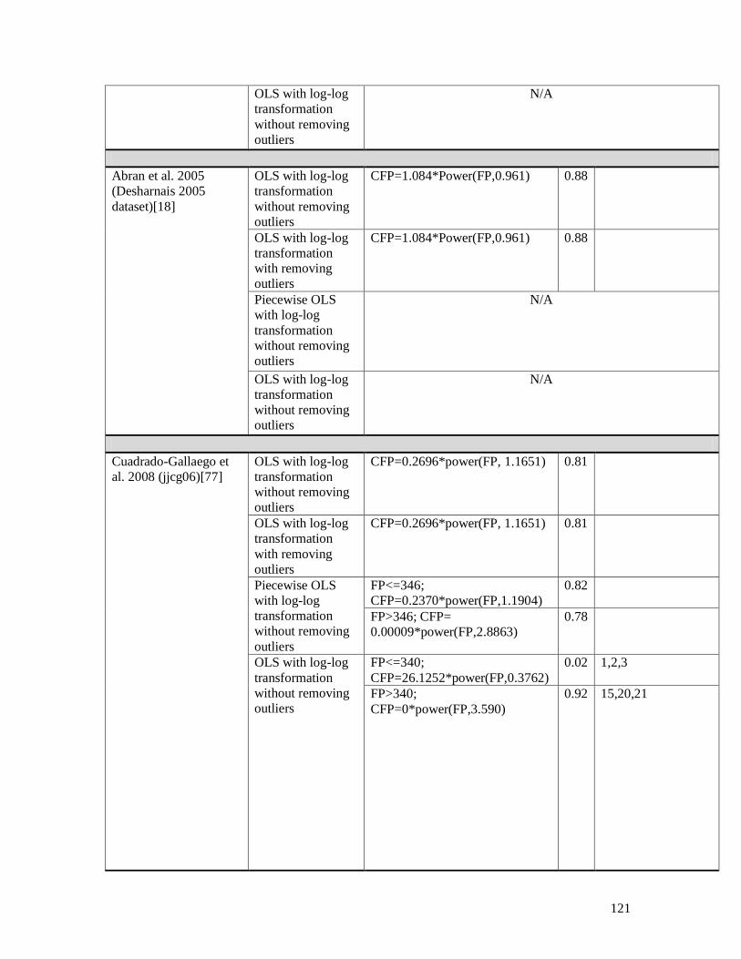
121
OLS with log-log
transformation
without removing
outliers
N/A
Abran et al. 2005
(Desharnais 2005
dataset)[18]
OLS with log-log
transformation
without removing
outliers
CFP=1.084*Power(FP,0.961) 0.88
OLS with log-log
transformation
with removing
outliers
CFP=1.084*Power(FP,0.961) 0.88
Piecewise OLS
with log-log
transformation
without removing
outliers
N/A
OLS with log-log
transformation
without removing
outliers
N/A
Cuadrado-Gallaego et
al. 2008 (jjcg06)[77]
OLS with log-log
transformation
without removing
outliers
CFP=0.2696*power(FP, 1.1651) 0.81
OLS with log-log
transformation
with removing
outliers
CFP=0.2696*power(FP, 1.1651) 0.81
Piecewise OLS
with log-log
transformation
without removing
outliers
FP<=346;
CFP=0.2370*power(FP,1.1904)
0.82
FP>346; CFP=
0.00009*power(FP,2.8863)
0.78
OLS with log-log
transformation
without removing
outliers
FP<=340;
CFP=26.1252*power(FP,0.3762)
0.02 1,2,3
FP>340;
CFP=0*power(FP,3.590)
0.92 15,20,21
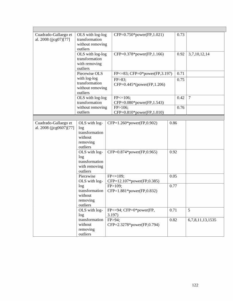
122
Cuadrado-Gallaego et
al. 2008 (jjcg0607)[77]
OLS with log-
log
transformation
without
removing
outliers
CFP=1.260*power(FP,0.902) 0.86
OLS with log-
log
transformation
with removing
outliers
CFP=0.874*power(FP,0.965) 0.92
Piecewise
OLS with log-
log
transformation
without
removing
outliers
FP<=109;
CFP=12.107*power(FP,0.385)
0.05
FP>109;
CFP=1.881*power(FP,0.832)
0.77
OLS with log-
log
transformation
without
removing
outliers
FP<=94; CFP=0*power(FP,
3.197)
0.71 5
FP>94;
CFP=2.3278*power(FP,0.794)
0.82 6,7,8,11,13,1535
Cuadrado-Gallaego et
al. 2008 (jjcg07)[77]
OLS with log-log
transformation
without removing
outliers
CFP=0.750*power(FP,1.021) 0.73
OLS with log-log
transformation
with removing
outliers
CFP=0.378*power(FP,1.166) 0.92 3,7,10,12,14
Piecewise OLS
with log-log
transformation
without removing
outliers
FP<=83; CFP=0*power(FP,3.197) 0.71
FP>83;
CFP=0.445*(power(FP,1.206)
0.75
OLS with log-log
transformation
without removing
outliers
FP<=106;
CFP=0.080*power(FP,1.543)
0.42 7
FP>106;
CFP=0.810*power(FP,1.010)
0.76
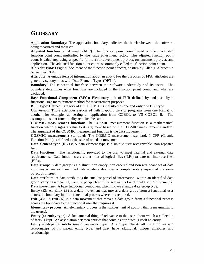
123
GLOSSARY
Application Boundary: The application boundary indicates the border between the software
being measured and the user.
Adjusted function point count (AFP): The function point count based on the unadjusted
function point count multiplied by the value adjustment factor. The adjusted function point
count is calculated using a specific formula for development project, enhancement project, and
application. The adjusted function point count is commonly called the function point count.
Albrecht 1984: Original document of the function point concept, written by Allan J. Albrecht in
November 1984.
Attribute: A unique item of information about an entity. For the purposes of FPA, attributes are
generally synonymous with Data Element Types (DET‘s).
Boundary: The conceptual interface between the software understudy and its users. The
boundary determines what functions are included in the function point count, and what are
excluded.
Base Functional Component (BFC): Elementary unit of FUR defined by and used by a
functional size measurement method for measurement purposes.
BFC Type: Defined Category of BFCs. A BFC is classified as one and only one BFC type.
Conversion: Those activities associated with mapping data or programs from one format to
another, for example, converting an application from COBOL to VS COBOL II. The
assumption is that functionality remains the same.
COSMIC measurement function: The COSMIC measurement function is a mathematical
function which assigns a value to its argument based on the COSMIC measurement standard.
The argument of the COSMIC measurement function is the data movement.
COSMIC measurement standard: The COSMIC measurement standard, 1 CFP (Cosmic
Function Point) is defined as the size of one data movement.
Data element type (DET): A data element type is a unique user recognizable, non-repeated
field.
Data functions: The functionality provided to the user to meet internal and external data
requirements. Data functions are either internal logical files (ILFs) or external interface files
(EIFs).
Data group: A data group is a distinct, non empty, non ordered and non redundant set of data
attributes where each included data attribute describes a complementary aspect of the same
object of interest.
Data attribute: A data attribute is the smallest parcel of information, within an identified data
group, carrying a meaning from the perspective of the software‘s Functional User Requirements.
Data movement: A base functional component which moves a single data group type.
Entry (E): An Entry (E) is a data movement that moves a data group from a functional user
across the boundary into the functional process where it is required.
Exit (X): An Exit (X) is a data movement that moves a data group from a functional process
across the boundary to the functional user that requires it.
Elementary process: An elementary process is the smallest unit of activity that is meaningful to
the user(s).
Entity (or entity type): A fundamental thing of relevance to the user, about which a collection
of facts is kept. An association between entities that contains attributes is itself an entity.
Entity subtype: A subdivision of an entity type. A subtype inherits all the attributes and
relationships of its parent entity type, and may have additional, unique attributes and
relationships.

124
External input (EI): An external input (EI) is an elementary process that processes data or
control information that comes from outside the application‘s boundary. The primary intent of
an EI is to maintain one or more ILFs and/or to alter the behavior of the system.
External inquiry (EQ): An external inquiry (EQ) is an elementary process that sends data or
control information outside the application boundary. The primary intent of an external inquiry
is to present information to a user through the retrieval of data or control information from an
ILF or EIF. The processing logic contains no mathematical formulas or calculations, and creates
no derived data. No ILF is maintained during the processing, nor is the behavior of the system
altered.
External interface file (EIF): An external interface file (EIF) is a user identifiable group of
logically related data or control information referenced by the application, but maintained within
the boundary of another application. The primary intent of an EIF is to hold data referenced
through one or more elementary processes within the boundary of the application counted. This
means an EIF counted for an application must be in an ILF in another application.
External output (EO):An external output (EO) is an elementary process that sends data or
control information outside the application‘s boundary. The primary intent of an external output
is to present information to a user through processing logic other than, or in addition to, the
retrieval of data or control information. The processing logic must contain at least one
mathematical formula or calculation, or create derived data. An external output may also
maintain one or more ILFs and/or alter the behavior of the system.
File:For data functions, a logically related group of data, not the physical implementation of
those groups of data.
File type referenced (FTR): A file type referenced is
• An internal logical file read or maintained by a transactional function or
• An external interface file read by a transactional function.
Functional User Requirements (FUR): A subset of user requirements, the FUR represents the
user practices and procedures that the software must perform to fulfill the users‘ needs. They
exclude quality requirements and any technical requirements. (ISO 14143-1)
Functional user: A (type of) user that is a sender and/or an intended recipient of data in the
Functional User Requirements of a piece of software.
Function point: A measure which represents the functional size of application software.
Function point analysis (FPA): A form of Functional Size Measurement (FSM) that measures
the work product of software development, change and maintenance activities associated with
Business Applications, from the customer's point of view.
Functional Size: (ISO Definition) A size of the software derived by quantifying the Functional
User Requirements.
Functional Size Measurement (FSM): (ISO Definition) The process of measuring Functional
Size.
Functional process: A functional process is an elementary component of a set of Functional
User Requirements comprising a unique, cohesive and independently executable set of data
movements. It is triggered by a data movement (an Entry) from a functional user that informs
the piece of software that the functional user has identified a triggering event. It is complete
when it has executed all that is required to be done in response to the triggering event.
Function point count: The function point measurement of a particular application or project.
Functional complexity: A specific function type's complexity rating which has a value of low,
average, or high. For data function types, the complexity is determined by the number of RETs
and DETs. For transactional function types, the complexity is determined by the number of
FTRs and DETs.
General system characteristics (GSCs): The general system characteristics are a set of 14
questions that evaluate the overall complexity of the application.

125
IFPUG: The International Function Point Users Group is a membership governed, non-profit
organization committed to promoting and supporting function point analysis and other software
measurement techniques.
Internal logical file (ILF): An internal logical file (ILF) is a user identifiable group of logically
related data or control information maintained within the boundary of the application. The
primary intent of an ILF is to hold data maintained through one or more elementary processes of
the application being counted.
Logical Transaction: The basic functional component of Mk II FPA. The smallest complete
unit of information processing that is meaningful to the end user in the business. It is triggered
by an event in the real world of interest to the user, or by a request for information. It comprises
an input, process and output component. It must be self-contained and leave the application
being counted in a consistent state.
Logical file: A logical group of permanent data seen from the perspective of the user. It is an
internal logical file or an external interface file. See also data function.
Maintained: The term maintained is the ability to modify data through an elementary process.
Measure: As a noun, a number that assigns relative value. Some examples may include volume,
height, function points, or work effort. As a verb, to ascertain or appraise by comparing to a
standard.
Measurement: Assigning relative value. Usually, in the improvement process, measures gained
from this activity are combined to form metrics.
NESMA: The Netherlands Software Metrics Association (www.nesma.org). A membership
governed non-profit organization in the Netherlands, committed to promoting and supporting
function point analysis and other software measurement methods.
Object of interest: Any ‗thing‘ that is identified from the point of view of the Functional User
Requirements. It may be any physical thing, as well as any conceptual object or part of a
conceptual object in the world of the functional user about which the software is required to
process and/or store data.
Project: A collection of work tasks with a time frame and a work product to be delivered.
Project/application attribute: Characteristics of a project or an application that may have a
significant impact on productivity. Examples include hardware platform, personnel experience,
tools, and methodology. The project/application attribute is used to categorize project data
during analysis.
Persistent storage: Persistent storage is storage which enables a functional process to store a
data group beyond the life of the functional process and/or from which a functional process can
retrieve a data group stored by another functional process, or stored by an earlier occurrence of
the same functional process, or stored by some other process.
Purpose of the Count: The purpose of a function point count is to provide an answer to a
business problem.
Purpose of a measurement: A statement that defines why a measurement is required, and what
the result will be used for.
Ratio: In the context of this document, ratio is defined as the result of dividing one measured
quantity by another.
Record: A group of related items that is treated as a unit.
Record element type (RET): A record element type (RET) is a user recognizable subgroup of
data elements within an ILF or EIF.
Read (R):A data movement that moves a data group from persistent storage within reach of the
functional process which requires it.
Scope of a measurement: The set of Functional User Requirements to be included in a specific
functional size measurement exercise.
126
Triggering event: An event (something that happens) that causes a functional user of the piece
of software to initiate (‗trigger‘) one or more functional processes. In a set of Functional User
Requirements, each event which causes a functional user to trigger a functional process
• cannot be sub-divided for that set of FUR, AND
• Has either happened or it has not happened.
Transactional functions: The functionality provided to the user to process data by an
application. Transactional functions are defined as external inputs, external outputs, and external
inquiries.
Technical Complexity Adjustment (TCA):A factor which attempts to take into account the
influence on application size of Technical and Quality Requirements, which may be used to
adjust the Function Point Index to give the Adjusted Functional Size. (The TCA is not included
within the ISO standard ISO/IEC 14143, nor is its use generally recommended).
Technical Complexity Adjustment Factors: The set of 19 factors that are taken into account in
the Technical Complexity Adjustment (TCA).Each factor has a Degree of Influence (DI) of
between 0and 5.
Unadjusted function point count (UFP): The measure of the functionality provided to the user
by the project or application. It is contributed by the measure of two function types—data and
transactional.
User: Any person that specifies Functional User Requirements and/or any person or thing that
communicates or interacts with the software at any time.
User recognizable / User identifiable: The term user identifiable refers to defined requirements
for processes and/or groups of data that are agreed upon, and understood by, both the user(s) and
software developer(s).
User perspective / User view: A user view represents a formal description of the user‘s
business needs in the user‘s language. Developers translate the user information into
information technology language in order to provide a solution.
Value adjustment factor (VAF): The factor that indicates the general functionality provided to
the user of the application. The VAF is calculated based on an assessment of the 14 general
system characteristics (GSCs) for an application.
Write (W): A data movement that moves a data group lying inside a functional process to
persistent storage.
Related Documents