A Comparison of Supervised Machine Learning Algorithms and Feature Vectors for MS Lesion Segmentation Using Multimodal Structural MRI

A Comparison of Supervised Machine LearningAlgorithms and Feature Vectors for MS LesionSegmentation Using Multimodal Structural MRIElizabeth M. Sweeney1,2*, Joshua T. Vogelstein3,4, Jennifer L. Cuzzocreo5, Peter A. Calabresi6,

Daniel S. Reich1,2,5,6, Ciprian M. Crainiceanu1, Russell T. Shinohara7

1 Department of Biostatistics, The Johns Hopkins University, Baltimore, Maryland, United States of America, 2 Translational Neuroradiology Unit, Neuroimmunology

Branch, National Institute of Neurological Disease and Stroke, National Institute of Health, Bethesda, Maryland, United States of America, 3 Department of Statistical

Science, Duke University, Durham, North Carolina, United States of America, 4 Center for the Developing Brain, Child Mind Institute, New York, New York, United States of

America, 5 Department of Radiology, The Johns Hopkins University School of Medicine, Baltimore, Maryland, United States of America, 6 Department of Neurology, The

Johns Hopkins University School of Medicine, Baltimore, Maryland, United States of America, 7 Department of Biostatistics and Epidemiology, Center for Clinical

Epidemiology and Biostatistics, Perelman School of Medicine, University of Pennsylvania, Philadelphia, Pennsylvania, United States of America

Abstract

Machine learning is a popular method for mining and analyzing large collections of medical data. We focus on a particularproblem from medical research, supervised multiple sclerosis (MS) lesion segmentation in structural magnetic resonanceimaging (MRI). We examine the extent to which the choice of machine learning or classification algorithm and featureextraction function impacts the performance of lesion segmentation methods. As quantitative measures derived fromstructural MRI are important clinical tools for research into the pathophysiology and natural history of MS, the developmentof automated lesion segmentation methods is an active research field. Yet, little is known about what drives performance ofthese methods. We evaluate the performance of automated MS lesion segmentation methods, which consist of asupervised classification algorithm composed with a feature extraction function. These feature extraction functions act onthe observed T1-weighted (T1-w), T2-weighted (T2-w) and fluid-attenuated inversion recovery (FLAIR) MRI voxel intensities.Each MRI study has a manual lesion segmentation that we use to train and validate the supervised classification algorithms.Our main finding is that the differences in predictive performance are due more to differences in the feature vectors, ratherthan the machine learning or classification algorithms. Features that incorporate information from neighboring voxels in thebrain were found to increase performance substantially. For lesion segmentation, we conclude that it is better to use simple,interpretable, and fast algorithms, such as logistic regression, linear discriminant analysis, and quadratic discriminantanalysis, and to develop the features to improve performance.

Citation: Sweeney EM, Vogelstein JT, Cuzzocreo JL, Calabresi PA, Reich DS, et al. (2014) A Comparison of Supervised Machine Learning Algorithms and FeatureVectors for MS Lesion Segmentation Using Multimodal Structural MRI. PLoS ONE 9(4): e95753. doi:10.1371/journal.pone.0095753

Editor: Bogdan Draganski, Centre Hospitalier Universitaire Vaudois Lausanne - CHUV, UNIL, Switzerland

Received January 3, 2014; Accepted March 28, 2014; Published April 29, 2014

This is an open-access article, free of all copyright, and may be freely reproduced, distributed, transmitted, modified, built upon, or otherwise used by anyone forany lawful purpose. The work is made available under the Creative Commons CC0 public domain dedication.

Funding: This research was partially supported by the Intramural Research Program of NINDS and NINDS R01 NS070906 and NINDS RO1 NS08521. The fundershad no role in study design, data collection and analysis, decision to publish, or preparation of the manuscript.

Competing Interests: The authors have declared that no competing interests exist.

* E-mail: [email protected]

Introduction

Machine learning is a popular perspective for mining and

analyzing large collections of medical data [1–3]. We focus on the

extent to which the choice of machine learning or classification

algorithm and the feature extraction function impact performance

in one problem from medical research – supervised multiple

sclerosis (MS) lesion segmentation in structural magnetic reso-

nance imaging (MRI). The evaluation of the classification

algorithms employed in supervised lesion segmentation methods

is not only a function of classification accuracy. Depending on the

application, computational efficiency and interpretability may be

valued at the cost of classification accuracy. Therefore, our

evaluation also includes the computational time and resources

required by each algorithm and the interpretability of the results

produced by the algorithm. Comparison of machine learning

techniques has been performed in other applications[4–6], but not

to our knowledge in multiple sclerosis lesion segmentation. Also

many of the currently available comparisons do not consider

computational time.

MS is a life-long chronic disease of the central nervous system

that is diagnosed primarily in young adults who will have a near

normal life expectancy. Because of this, the burden of the disease is

great, with large economic, social and medical costs. Between

250,000 and 400,000 people in the United States have been

diagnosed with MS, and the estimated annual cost of the disease is

over six billion dollars. There is currently no cure for MS, but

many therapies exist for treating symptoms and delaying

accumulation of permanent disability (http://www.ninds.nih.

gov/disorders/multiple_ sclerosis/detail_multiple_sclerosis.htm).

MS is characterized by demylinating lesions that are predomi-

nately located in the white matter of the brain, and MRI of the

brain is sensitive to these lesions [7]. Quantitative MRI metrics,

such as the number and volume of lesions, are important clinical

tools for research into the pathophysiology and natural history of

PLOS ONE | www.plosone.org 1 April 2014 | Volume 9 | Issue 4 | e95753

http://www.ninds.nih.gov/disorders/multiple_

http://www.ninds.nih.gov/disorders/multiple_

http://crossmark.crossref.org/dialog/?doi=10.1371/journal.pone.0095753&domain=pdf

MS [8]. In practice, lesion burden is determined by manual or

semi-automated examination and delineation of MRI, which is

time consuming, costly, and prone to large inter- and intra-

observer variability [9]. Therefore development of automated MS

lesion segmentation methods is an active research field [8,10]. The

problem of automated MS lesion segmentation must be addressed

by a method that is both sensitive and specific to white matter

lesions, and which generalizes across subjects and imaging centers.

Many machine learning algorithms have been developed for

automated segmentation of MS lesions in structural MRI. Over 80

papers have been published on the topic in the last 15 years, and

yet no solution to this problem has emerged as superior to other

methods [10]. Each lesion segmentation method in the literature is

the composition of a classification algorithm and feature extraction

function applied to one or many MRI modalities. As different

methods use different data sets and performance metrics, the

extent to which the classification algorithm, the feature extraction

function, and the interplay between the classification algorithm

and feature extraction function impacts the performance of these

methods is unknown. To investigate this, we examine which

factors improve classification performance through the composi-

tion of nine supervised classification algorithms with six feature

extraction functions. We use voxel intensities form the T1-

weighted (T1-w), T2-weighted (T2-w) and fluid-attenuated inver-

sion recovery (FLAIR) MRI modalities to train and validate

performance of the combinations of classifiers and feature

extraction functions. We are not proposing a new lesion

segmentation method. Rather than searching for the optimal

method, we explore the problem and present our insights into the

tools and methods of approach.

Our findings are that, for the employed feature extraction

methods, the particular classification algorithm is much less

important than the careful development of the features. These

findings are not unique to this problem. Hand (2006) asserts that,

in practice, in classification, simple classifiers typically yield

performance almost as good or better than more sophisticated

classifiers [11]. This is attributed to sources of uncertainty in data

that are generally not considered in the classical supervised

classification paradigm. Hand refers to using complex classification

algorithms as ‘‘the illusion of progress’’. Our findings support this

characterization.

Experimental Methods

Ethics StatementThe Johns Hopkins Medicine IRB acknowledged the collection

and analysis of data presented in this manuscript qualifies as

exempt research under the Department of Health and Human

Services regulations. MRI and clinical data were previously

collected as part of IRB approved research studies with written

consent provided by participants. The identifiable MRI and

clinical information accessed by the principal investigator were

recorded in such a manner that subjects cannot be identified,

directly or through identifiers linked to the subjects (e.g., no codes

or links were retained to allow re-identification of individuals).

Study Population and Experimental MethodsWe consider MRI studies with T1-w, T2-w and FLAIR volumes

from 98 patients with MS. The 3D T1-MPRAGE images

(repetition time (TR) = 10 ms; echo time (TE) = 6 ms; flip angle

(FA) a~80; inversion time (TI) = 835 ms, resolution = 1.1 mm

|1.1 mm |1.1 mm), 2D T2-w FLAIR images (TR = 11000 ms;

TE = 68 ms; TI = 2800 ms; in-plane resolution = 0.83 mm |0.83 mm; slice thickness = 2.2 mm) and T2-w volumes(TR

= 4200 ms; TE = 80 ms; resolution = 0.83 mm |0.83 mm

|2.2 mm) were acquired on a 3 tesla MRI scanner (Philips

Medical Systems, Best, The Netherlands) equipped with an 8-

channel phased array head coil.

Image PreprocessingWe preprocessed the MRI images using the tools provided in

Medical Image Processing Analysis and Visualization (MIPAV)

[12], TOADS-CRUISE (http://www.nitrc.org/projects/toads-

cruise/), and Java Image Science Toolkit (JIST) [13] software

packages. We first rigidly aligned the T1-w image of each subject

into the Montreal Neurological Institute (MNI) standard space

(voxel resolution 1 mm3). We then registered the FLAIR and T2-

w images of each subject to the aligned T1-w images. We also

applied the N3 inhomogeneity correction algorithm [14] to all

images and removed extracerebral voxels using SPECTRE, a

skull-stripping procedure [15]. A brain tissue mask is created from

the extracerebral voxel removal mask by removing voxels falling

below the 15th percentile of the FLAIR intensities over the mask

[16]. This brain tissue mask removes cerebrospinal fluid in the

ventricles and outside the brain.

Statistical Methods

Our aim is to examine the extent to which the classification

algorithm and the feature extraction function impacts the

performance of lesion segmentation methods. To do so, we

compare compositions of supervised classification algorithms and

feature extraction functions for the classification of lesion voxels

versus healthy tissue in structural MRI studies. A feature

extraction function is a function that acts on the observed

intensities from the MRI modalities and produces a feature vector.

For each voxel of the brain, we have a ‘‘silver standard’’ manual

lesion segmentation used to train and validate the lesion

segmentation method. Manual lesion segmentations are consid-

ered a silver standard, as opposed to ground truth, as there is

much inter- and intra- observer variability amongst expert

segmentations. We examine lesion segmentation methods that

are the composition of a classification algorithm and a feature

extraction function. Here, our goal is not to find an the optimal

lesion segmentation method; we instead search for insight by

evaluating the performance over a set of possible classifiers and

extraction functions.

Supervised Classification AlgorithmsVoxels within a brain are spatially correlated. To include spatial

information, we also include functions of voxel neighborhoods as

features in our voxel-level classifiers. The extent to which the

residuals are still correlated after these features are included or to

what extent this information can be used to further improve

prediction remain open problems.

We provide a short description of the super learner, as this is not

a standard classification technique employed in the neuroimaging

literature. The super learner is a method for combining class

estimations from different classification algorithms, by weighting

the classifiers according to their prediction performance using a

cross-validation loss function [17–20], which is referred to in the

literature as ensemble learning, model stacking, or super learning.

The super learner assigns each classification algorithm a coefficient

weight, ai[(0,1), withP

i ai~1. A more detailed description of the

super learner and of the other supervised classification algorithms

used in this analysis can be found in the Appendix S1.

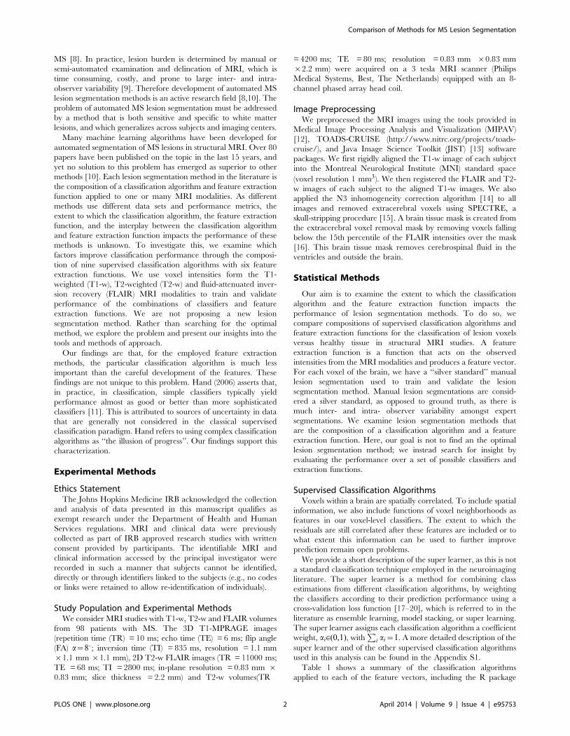
Table 1 shows a summary of the classification algorithms

applied to each of the feature vectors, including the R package

Comparison of Methods for MS Lesion Segmentation


http://www.nitrc.org/projects/toads-cruise/

http://www.nitrc.org/projects/toads-cruise/

used to apply the algorithm and, when applicable, the tuning

parameter values that were searched over. We performed all

modeling in the R environment (version 2.15.3, R Foundation for

Statistical Computing, Vienna, Austria) with the packages

AnalyzeFMRI [21], ROCR [22], MASS [23], class [23], nnet

[23], mclust [24,25], e1071 [26], randomForest [27], and

SuperLearner [28].

Feature Extraction Functions and VectorsIn this section we introduce the six feature extraction functions

and the vectors these functions produce. In Figure 1, we examine

3-dimensional scatter plots of the intensities of the features that

form the feature vectors. Note that while many of the feature

vectors are in a higher dimension, in this figure we are only able to

show 3-dimensions. Scatter plots of the T1-w, T2-w and FLAIR

intensities and functions of these intensities for 10,000 randomly

sampled voxels of 5 randomly sampled subject’s MRI studies (a

total of 50,000 voxels) are shown; each point in the plot represents

a single voxel from a MRI study. We will refer to this figure

throughout this section. Table 2 contains a summary of the feature

vectors introduced in this section.

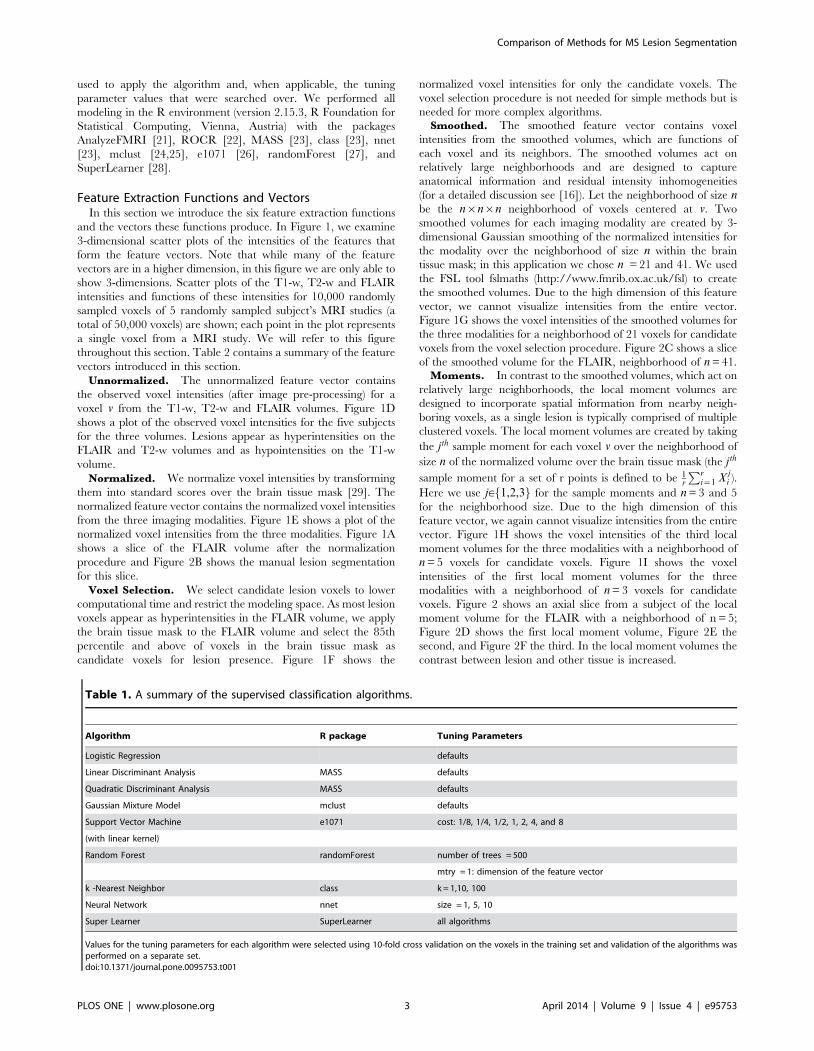
Unnormalized. The unnormalized feature vector contains

the observed voxel intensities (after image pre-processing) for a

voxel v from the T1-w, T2-w and FLAIR volumes. Figure 1D

shows a plot of the observed voxel intensities for the five subjects

for the three volumes. Lesions appear as hyperintensities on the

FLAIR and T2-w volumes and as hypointensities on the T1-w

volume.

Normalized. We normalize voxel intensities by transforming

them into standard scores over the brain tissue mask [29]. The

normalized feature vector contains the normalized voxel intensities

from the three imaging modalities. Figure 1E shows a plot of the

normalized voxel intensities from the three modalities. Figure 1A

shows a slice of the FLAIR volume after the normalization

procedure and Figure 2B shows the manual lesion segmentation

for this slice.

Voxel Selection. We select candidate lesion voxels to lower

computational time and restrict the modeling space. As most lesion

voxels appear as hyperintensities in the FLAIR volume, we apply

the brain tissue mask to the FLAIR volume and select the 85th

percentile and above of voxels in the brain tissue mask as

candidate voxels for lesion presence. Figure 1F shows the

normalized voxel intensities for only the candidate voxels. The

voxel selection procedure is not needed for simple methods but is

needed for more complex algorithms.Smoothed. The smoothed feature vector contains voxel

intensities from the smoothed volumes, which are functions of

each voxel and its neighbors. The smoothed volumes act on

relatively large neighborhoods and are designed to capture

anatomical information and residual intensity inhomogeneities

(for a detailed discussion see [16]). Let the neighborhood of size nbe the n|n|n neighborhood of voxels centered at v. Two

smoothed volumes for each imaging modality are created by 3-

dimensional Gaussian smoothing of the normalized intensities for

the modality over the neighborhood of size n within the brain

tissue mask; in this application we chose n = 21 and 41. We used

the FSL tool fslmaths (http://www.fmrib.ox.ac.uk/fsl) to create

the smoothed volumes. Due to the high dimension of this feature

vector, we cannot visualize intensities from the entire vector.

Figure 1G shows the voxel intensities of the smoothed volumes for

the three modalities for a neighborhood of 21 voxels for candidate

voxels from the voxel selection procedure. Figure 2C shows a slice

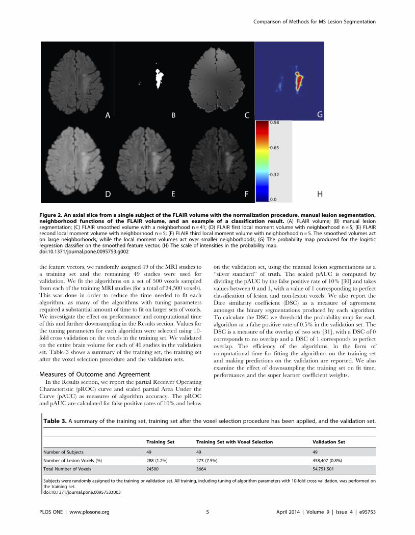
of the smoothed volume for the FLAIR, neighborhood of n = 41.Moments. In contrast to the smoothed volumes, which act on

relatively large neighborhoods, the local moment volumes are

designed to incorporate spatial information from nearby neigh-

boring voxels, as a single lesion is typically comprised of multiple

clustered voxels. The local moment volumes are created by taking

the jth sample moment for each voxel v over the neighborhood of

size n of the normalized volume over the brain tissue mask (the jth

sample moment for a set of r points is defined to be 1r

Pri~1 X

ji ).

Here we use j[f1,2,3g for the sample moments and n = 3 and 5

for the neighborhood size. Due to the high dimension of this

feature vector, we again cannot visualize intensities from the entire

vector. Figure 1H shows the voxel intensities of the third local

moment volumes for the three modalities with a neighborhood of

n = 5 voxels for candidate voxels. Figure 1I shows the voxel

intensities of the first local moment volumes for the three

modalities with a neighborhood of n = 3 voxels for candidate

voxels. Figure 2 shows an axial slice from a subject of the local

moment volume for the FLAIR with a neighborhood of n = 5;

Figure 2D shows the first local moment volume, Figure 2E the

second, and Figure 2F the third. In the local moment volumes the

contrast between lesion and other tissue is increased.

Table 1. A summary of the supervised classification algorithms.

Algorithm R package Tuning Parameters

Logistic Regression defaults

Linear Discriminant Analysis MASS defaults

Quadratic Discriminant Analysis MASS defaults

Gaussian Mixture Model mclust defaults

Support Vector Machine e1071 cost: 1/8, 1/4, 1/2, 1, 2, 4, and 8

(with linear kernel)

Random Forest randomForest number of trees = 500

mtry = 1: dimension of the feature vector

k -Nearest Neighbor class k = 1,10, 100

Neural Network nnet size = 1, 5, 10

Super Learner SuperLearner all algorithms

Values for the tuning parameters for each algorithm were selected using 10-fold cross validation on the voxels in the training set and validation of the algorithms wasperformed on a separate set.doi:10.1371/journal.pone.0095753.t001



http://www.fmrib.ox.ac.uk/fsl

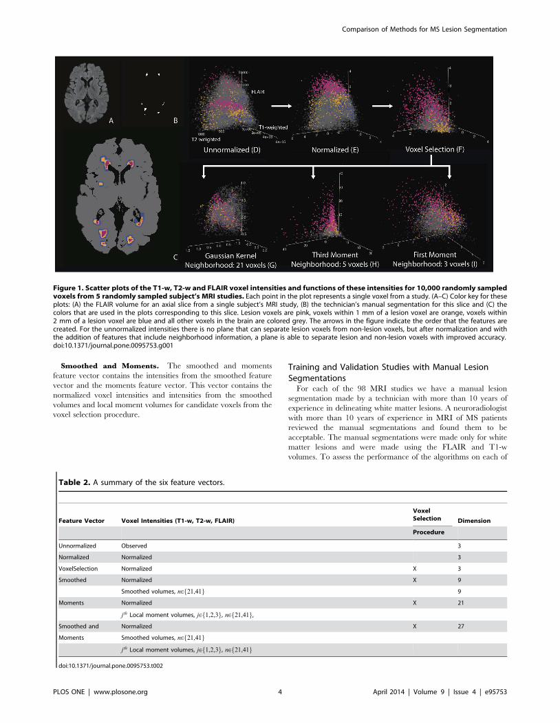
Smoothed and Moments. The smoothed and moments

feature vector contains the intensities from the smoothed feature

vector and the moments feature vector. This vector contains the

normalized voxel intensities and intensities from the smoothed

volumes and local moment volumes for candidate voxels from the

voxel selection procedure.

Training and Validation Studies with Manual LesionSegmentations

For each of the 98 MRI studies we have a manual lesion

segmentation made by a technician with more than 10 years of

experience in delineating white matter lesions. A neuroradiologist

with more than 10 years of experience in MRI of MS patients

reviewed the manual segmentations and found them to be

acceptable. The manual segmentations were made only for white

matter lesions and were made using the FLAIR and T1-w

volumes. To assess the performance of the algorithms on each of

Figure 1. Scatter plots of the T1-w, T2-w and FLAIR voxel intensities and functions of these intensities for 10,000 randomly sampledvoxels from 5 randomly sampled subject’s MRI studies. Each point in the plot represents a single voxel from a study. (A–C) Color key for theseplots: (A) the FLAIR volume for an axial slice from a single subject’s MRI study, (B) the technician’s manual segmentation for this slice and (C) thecolors that are used in the plots corresponding to this slice. Lesion voxels are pink, voxels within 1 mm of a lesion voxel are orange, voxels within2 mm of a lesion voxel are blue and all other voxels in the brain are colored grey. The arrows in the figure indicate the order that the features arecreated. For the unnormalized intensities there is no plane that can separate lesion voxels from non-lesion voxels, but after normalization and withthe addition of features that include neighborhood information, a plane is able to separate lesion and non-lesion voxels with improved accuracy.doi:10.1371/journal.pone.0095753.g001

Table 2. A summary of the six feature vectors.

Feature Vector Voxel Intensities (T1-w, T2-w, FLAIR)

VoxelSelection Dimension

Procedure

Unnormalized Observed 3

Normalized Normalized 3

VoxelSelection Normalized X 3

Smoothed Normalized X 9

Smoothed volumes, n[f21,41g 9

Moments Normalized X 21

jth Local moment volumes, j[f1,2,3g, n[f21,41g,Smoothed and Normalized X 27

Moments Smoothed volumes, n[f21,41g

jth Local moment volumes, j[f1,2,3g, n[f21,41g

doi:10.1371/journal.pone.0095753.t002



the feature vectors, we randomly assigned 49 of the MRI studies to

a training set and the remaining 49 studies were used for

validation. We fit the algorithms on a set of 500 voxels sampled

from each of the training MRI studies (for a total of 24,500 voxels).

This was done in order to reduce the time needed to fit each

algorithm, as many of the algorithms with tuning parameters

required a substantial amount of time to fit on larger sets of voxels.

We investigate the effect on performance and computational time

of this and further downsampling in the Results section. Values for

the tuning parameters for each algorithm were selected using 10-

fold cross validation on the voxels in the training set. We validated

on the entire brain volume for each of 49 studies in the validation

set. Table 3 shows a summary of the training set, the training set

after the voxel selection procedure and the validation sets.

Measures of Outcome and AgreementIn the Results section, we report the partial Receiver Operating

Characteristic (pROC) curve and scaled partial Area Under the

Curve (pAUC) as measures of algorithm accuracy. The pROC

and pAUC are calculated for false positive rates of 10% and below

on the validation set, using the manual lesion segmentations as a

‘‘silver standard’’ of truth. The scaled pAUC is computed by

dividing the pAUC by the false positive rate of 10% [30] and takes

values between 0 and 1, with a value of 1 corresponding to perfect

classification of lesion and non-lesion voxels. We also report the

Dice similarity coefficient (DSC) as a measure of agreement

amongst the binary segmentations produced by each algorithm.

To calculate the DSC we threshold the probability map for each

algorithm at a false positive rate of 0.5% in the validation set. The

DSC is a measure of the overlap of two sets [31], with a DSC of 0

corresponds to no overlap and a DSC of 1 corresponds to perfect

overlap. The efficiency of the algorithms, in the form of

computational time for fitting the algorithms on the training set

and making predictions on the validation are reported. We also

examine the effect of downsampling the training set on fit time,

performance and the super learner coefficient weights.

Figure 2. An axial slice from a single subject of the FLAIR volume with the normalization procedure, manual lesion segmentation,neighborhood functions of the FLAIR volume, and an example of a classification result. (A) FLAIR volume; (B) manual lesionsegmentation; (C) FLAIR smoothed volume with a neighborhood n = 41; (D) FLAIR first local moment volume with neighborhood n = 5; (E) FLAIRsecond local moment volume with neighborhood n = 5; (F) FLAIR third local moment volume with neighborhood n = 5. The smoothed volumes acton large neighborhoods, while the local moment volumes act over smaller neighborhoods; (G) The probability map produced for the logisticregression classifier on the smoothed feature vector; (H) The scale of intensities in the probability map.doi:10.1371/journal.pone.0095753.g002

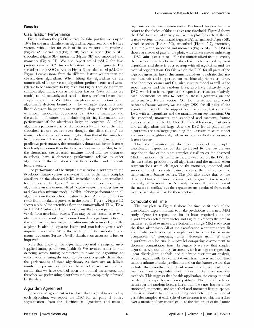
Table 3. A summary of the training set, training set after the voxel selection procedure has been applied, and the validation set.

Training Set Training Set with Voxel Selection Validation Set

Number of Subjects 49 49 49

Number of Lesion Voxels (%) 288 (1.2%) 273 (7.5%) 458,407 (0.8%)

Total Number of Voxels 24500 3664 54,751,501

Subjects were randomly assigned to the training or validation set. All training, including tuning of algorithm parameters with 10-fold cross validation, was performed onthe training set.doi:10.1371/journal.pone.0095753.t003



Results

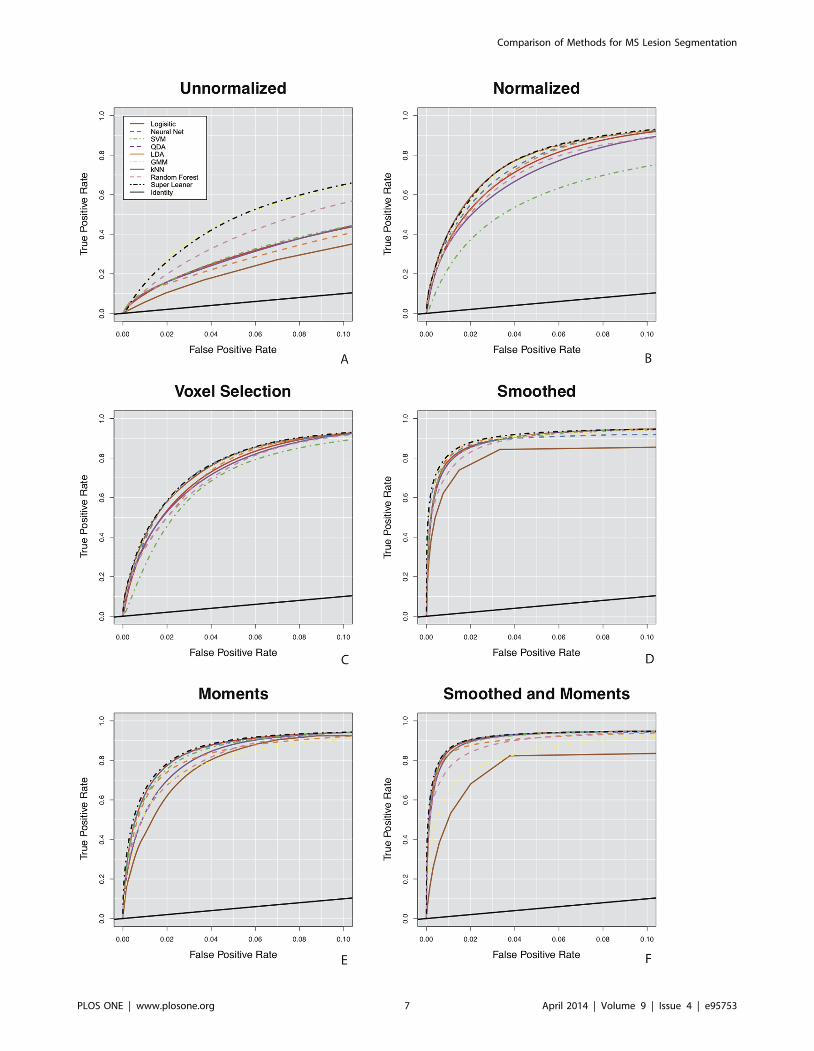
Classification PerformanceFigure 3 shows the pROC curves for false positive rates up to

10% for the nine classification algorithms organized by the feature

vectors, with a plot for each of the six vectors: unnormalized

(Figure 3A), normalized (Figure 3B), voxel selection (Figure 3C),

smoothed (Figure 3D), moments, (Figure 3E) and smoothed and

moments (Figure 3F). We also report scaled pAUC for false

positive rates of 10% for each feature vector in Figure 4. The

spread in the pROC curves in Figure 3 and the scaled pAUC in

Figure 4 comes more from the different feature vectors than the

classification algorithms. When fitting the algorithms on the

unnormalized feature vector, algorithms perform better and worse

relative to one another. In Figures 3 and Figure 4 we see that more

complex algorithms, such as the super learner, Gaussian mixture

model, neural network, and random forest, perform better than

simpler algorithms. We define complexity as a function of an

algorithm’s decision boundary – for example algorithms with

linear decision boundaries are relatively simpler than algorithm

with nonlinear decision boundaries [32]. After normalization and

the addition of features that include neighboring information, the

performance of the algorithms begin to converge. All of the

algorithms perform worse on the moments feature vector than the

smoothed feature vector, even thought the dimension of the

moments feature vector is much higher than that of the smoothed

feature vector (21 versus 9). In this application and in terms of

predictive performance, the smoothed volumes are better features

for classifying lesions than the local moment volumes. Also, two of

the algorithms, the Gaussian mixture model and the k-nearest

neighbors, have a decreased performance relative to other

algorithms on the validation set in the smoothed and moments

feature vector.

The performance of the simpler classification algorithms on the

developed feature vectors is superior to that of the more complex

classifiers on the observed MRI intensities in the unnormalized

feature vector. In Figure 3 we see that the best performing

algorithms on the unnormalized feature vector, the super learner

and Gaussian mixture model, exhibit inferior performance to all

algorithms on the developed feature vectors. An intuition for this

result from the data is provided in the plots of Figure 1. Figure 1D

shows a plot of the intensities from the unnormalized T1-w, T2-w

and FLAIR volumes. There is no plane that can separate lesion

voxels from non-lesion voxels. This may be the reason as to why

algorithms with nonlinear decision boundaries perform better on

the unnormalized feature vector. After normalization in Figure 1E,

a plane is able to separate lesion and non-lesion voxels with

improved accuracy. With the addition of the smoothed and

moment volumes (Figure 1G–H), classification accuracy is further

improved.

Note that many of the algorithms required a range of user-

supplied tuning parameters (Table 3). We invested much time in

deciding which tuning parameters to allow the algorithms to

search over, as using the incorrect parameters greatly diminished

the performance of these algorithms. As there are an infinite

number of parameters than can be searched, we can never be

certain that we have decided upon the optimal parameters, and

therefore we prefer using algorithms that are completely informed

by the data.

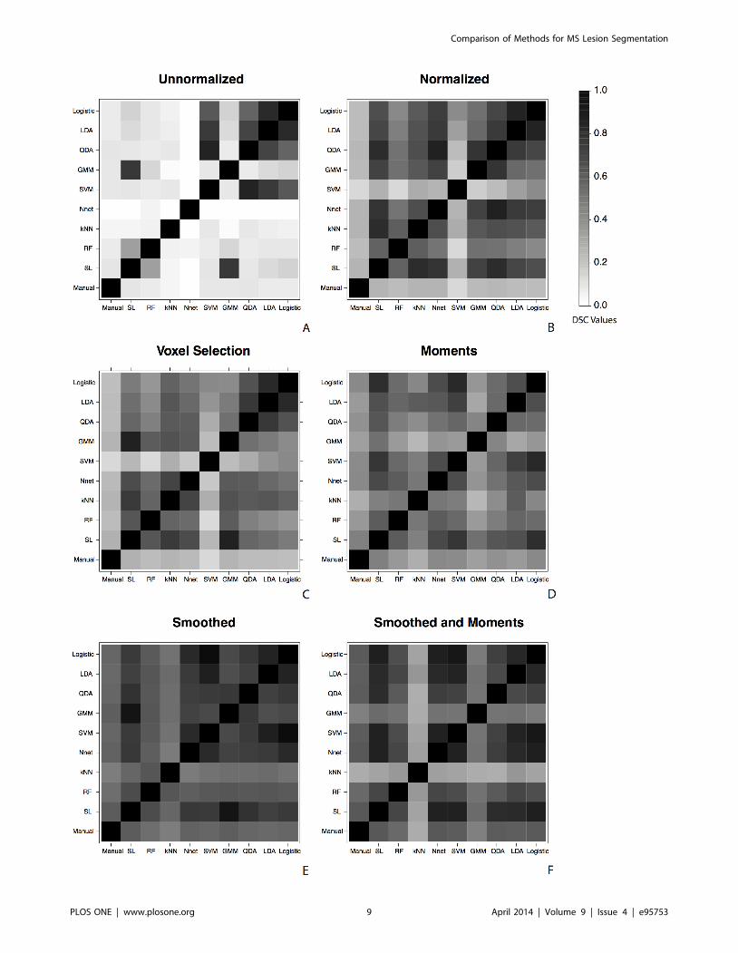
Algorithm AgreementTo assess the agreement in the class label assigned to a voxel by

each algorithm, we report the DSC for all pairs of binary

segmentations from the classification algorithms and manual

segmentations on each feature vector. We found these results to be

robust to the choice of false positive rate threshold. Figure 5 shows

the DSC for each of these pairs, with a plot for each of the six

feature vectors: unnormalized (Figure 5A), normalized (Figure 5B),

voxel selection (Figure 5C), smoothed (Figure 5D), moments,

(Figure 5E) and smoothed and moments (Figure 5F). The DSC is

shown as shades of gray in the plots, with darker shades indicating

a DSC value closer to one. For the unnormalized feature vector,

there is poor overlap between the class labels assigned by most

algorithms and there is poor overlap with all algorithms and the

manual segmentation. On this vector, the DSC for all pairs of the

logistic regression, linear discriminant analysis, quadratic discrim-

inant analysis and support vector machine algorithms are large.

Also the super learner and Gaussian mixture model as well as the

super learner and the random forest also have relatively large

DSC, which is to be excepted as the super learner assigns relatively

high coefficient weights to both of these algorithms on the

unnormalized feature vector. On the normalized and voxel

selection feature vectors, we see high DSC for all pairs of the

algorithms, excluding the support vector machine, but see a low

DSC with all algorithms and the manual lesion segmentation. On

the smoothed, moments, and smoothed and moments feature

vectors we see that the DSC for the manual lesion segmentations

and all algorithms are large. Also the DSC for all pairs of the

algorithms are also large (excluding the Gaussian mixture model

and k-nearest neighbors algorithms on the smoothed and moments

feature vector).

This plot reiterates that the performance of the simpler

classification algorithms on the developed feature vectors are

superior to that of the more complex classifiers on the observed

MRI intensities in the unnormalized feature vector; the DSC for

the class labels produced by all algorithms and the manual lesion

segmentations are much larger on the moments, smoothed, and

smoothed and moments feature vectors than those on the

unnormalized feature vectors. The plot also shows that on the

developed feature vectors, the class labels assigned to the voxels for

each algorithm are similar. Not only are overall performance of

the methods similar, but the segmentations produced from each

method are also similar for these vectors.

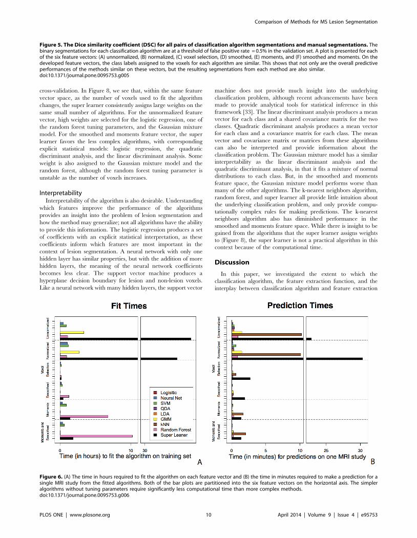
Computational TimeThe bar plots in Figure 6 show the time to fit each of the

classification algorithms and to make predictions on a new MRI

study; Figure 6A reports the time in hours required to fit the

algorithm on each feature vector and Figure 6B reports the time in

minutes required to make a prediction for a single MRI study from

the fitted algorithms. All of the classification algorithms were fit

and made predictions on a single core to allow for accurate

comparison of computing times, although many of these

algorithms can be run in a parallel computing environment to

decrease computation time. In Figure 6 we see that simpler

algorithms without tuning parameters, such as logistic regression,

linear discriminant analysis, and quadratic discriminant analysis,

require significantly less computational time. These methods take

under a minute to make predictions and on the feature vectors that

include the smoothed and local moment volumes and these

methods have comparable performance to the more complex

methods. This suggests that for this application, the computational

burden of the super learner is not justifiable. Note that the relative

fit time for the random forest is larger than the super learner in the

smoothed, moments, and smoothed and moments feature spaces.

This is attributed to the mtry tuning parameter, the number of

variables sampled at each split of the decision tree, which searches

over a number of parameters equal to the dimension of the feature





vector. The random forest takes longer to tune than the super

learner in this space and this difference can be attributed to the

respective packages implementation of model tuning; the Super-

Learner package calls the randomForest package to fit the random

forest, but selects tuning parameters internally.

Computational time to fit the algorithm on the training data

and make predictions for a new MRI study is an important

consideration when choosing the appropriate classification algo-

rithm in the application of lesion segmentation. This is especially

important for making predictions for a new MRI study (Figure 6B).

The algorithm may only need to be trained once and, as shown in

this application, and can be trained on a relatively small number of

voxels to reduce computational time. In research or clinical

settings, fast algorithm predictions are desired, as lesion segmen-

tations may be required for hundreds or thousands of studies. The

two algorithms with the best predictive performance on the

normalized feature vector, the super learner and the k –nearest

neighbors, would not scale well; the algorithms take 10 and 30

minutes respectively to make predictions for a new MRI study.

Even on the feature vectors that use the voxel selection procedure,

k-nearest neighbors and the super learner often take between two

to three minutes to make predictions for a single MRI study, while

many of the other algorithms take only a few seconds to make

these predictions.

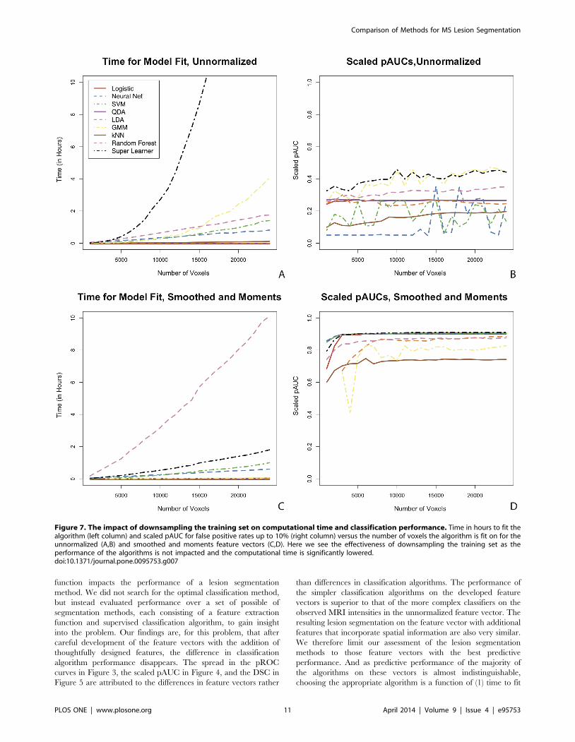
Downsampling the Training Set: ClassificationPerformance and Computational Time

In Figure 7 we investigate the impact of the number of voxels

used to fit the algorithms on prediction accuracy and computation

time. We examine the scaled pAUC for false positive rates up to

10% and the time to fit the algorithm on the unnormalized and

smoothed and moments feature vectors. We sample 1,000 to

24,000 voxels (without replacement) by increments of 1,000 from

the 24,500 voxels in the training set and fit the algorithms on each

of these samples. Figure 7A shows the scaled pAUC versus the

number of voxels the algorithm is fit on for the unnormalized

feature vector and Figure 7B shows the time to fit the algorithm.

Figure 7C and Figure 7D show the same for the smoothed and

moments feature vector. At 10 hours we cut off the algorithm fit

time on the plots; the super learner on the unnormalized feature

vector took approximately 30 hours to fit on 24,000 voxels. The

vertical axis for the smoothed and moments feature vector shows

the number of voxels before the candidate voxel selection

procedure is performed, as this procedure is part of the feature

vector space, so the actual number of voxels the algorithm is fit on

is around 15% of this size.

In Figure 7 we see the effectiveness of downsampling the

training set to reduce computational time, without impacting

performance. The performance of the algorithms is not impacted

and the computational time is significantly lowered. On the

unnormalized feature vector (Figure 7B) the performance of some

algorithms varies as the number of voxels increases, especially the

support vector machine and the neural network. On the smoothed

and moments feature vector the performance is much more

consistent. After the algorithm is fit on around 3000 voxels, the

scaled pAUC for the validation set is stable as the number of voxel

the algorithm is fit on increases. This shows that downsampling the

training set can be an effective tool for reducing computation time

without loss of performance on a well developed feature vector. In

Figure 7A and C we see that in the unnormalized feature vector

space the fit times for the k-nearest neighbors, quadratic

discriminant analysis, linear discriminant analysis, and logistic

regression appear to stay relatively constant as the number of

voxels on which the algorithm is fit increases from 1000 to 24,000.

The random forest, support vector machine, and neural network

appear to increase linearly in computation time and the super

learner and Gaussian mixture algorithm both appear to increase

exponentially. The required time for the super learner, support

vector machine, and neural network increase linearly and the

others stay relatively constant.

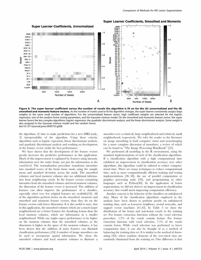
Super Learner CoefficientsWe examined the coefficient weights from the super learner

algorithm in Figure 8. Figure 8A shows the weights, as shades of

gray (darker indicating higher weight), on the unnormalized

feature vector and Figure 8B shows the weights for the smoothed

and moments feature vector. The weights are examined versus the

number of voxels fit by the algorithm, as in Figure 7. The

horizontal axis of the plots show the algorithms and tuning

parameters and the vertical axis shows the number of voxels on

which the algorithm was fit. The super learner is designed to select

and combine the classification algorithms that perform best, by

Figure 3. The partial Receiver Operating Characteristic (pROC) curves for the classification algorithms for false positive rates up to10% in the validation set. The diagonal line is shown on each plot in black for reference, and represents a classifier that performs as well aschance. A plot is presented for each of the six feature vectors: (A) unnormalized, (B) normalized, (C) voxel selection, (D) smoothed, (E) moments, and(F) smoothed and moments. The performance of the simpler classification algorithms on the feature vectors with features including spatialinformation are superior to that of the more complex classifiers on the original features on the unnormalized feature vector.doi:10.1371/journal.pone.0095753.g003

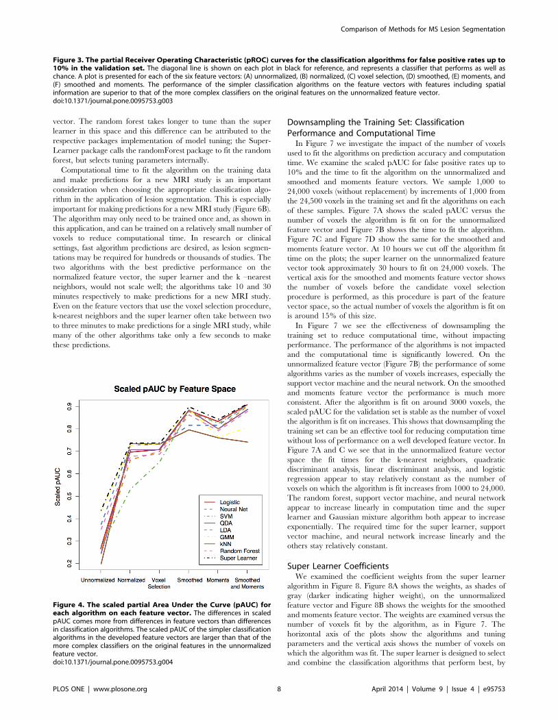
Figure 4. The scaled partial Area Under the Curve (pAUC) foreach algorithm on each feature vector. The differences in scaledpAUC comes more from differences in feature vectors than differencesin classification algorithms. The scaled pAUC of the simpler classificationalgorithms in the developed feature vectors are larger than that of themore complex classifiers on the original features in the unnormalizedfeature vector.doi:10.1371/journal.pone.0095753.g004





cross-validation. In Figure 8, we see that, within the same feature

vector space, as the number of voxels used to fit the algorithm

changes, the super learner consistently assigns large weights on the

same small number of algorithms. For the unnormalized feature

vector, high weights are selected for the logistic regression, one of

the random forest tuning parameters, and the Gaussian mixture

model. For the smoothed and moments feature vector, the super

learner favors the less complex algorithms, with corresponding

explicit statistical models: logistic regression, the quadratic

discriminant analysis, and the linear discriminant analysis. Some

weight is also assigned to the Gaussian mixture model and the

random forest, although the random forest tuning parameter is

unstable as the number of voxels increases.

InterpretabilityInterpretability of the algorithm is also desirable. Understanding

which features improve the performance of the algorithms

provides an insight into the problem of lesion segmentation and

how the method may generalize; not all algorithms have the ability

to provide this information. The logistic regression produces a set

of coefficients with an explicit statistical interpretation, as these

coefficients inform which features are most important in the

context of lesion segmentation. A neural network with only one

hidden layer has similar properties, but with the addition of more

hidden layers, the meaning of the neural network coefficients

becomes less clear. The support vector machine produces a

hyperplane decision boundary for lesion and non-lesion voxels.

Like a neural network with many hidden layers, the support vector

machine does not provide much insight into the underlying

classification problem, although recent advancements have been

made to provide analytical tools for statistical inference in this

framework [33]. The linear discriminant analysis produces a mean

vector for each class and a shared covariance matrix for the two

classes. Quadratic discriminant analysis produces a mean vector

for each class and a covariance matrix for each class. The mean

vector and covariance matrix or matrices from these algorithms

can also be interpreted and provide information about the

classification problem. The Gaussian mixture model has a similar

interpretability as the linear discriminant analysis and the

quadratic discriminant analysis, in that it fits a mixture of normal

distributions to each class. But, in the smoothed and moments

feature space, the Gaussian mixture model performs worse than

many of the other algorithms. The k-nearest neighbors algorithm,

random forest, and super learner all provide little intuition about

the underlying classification problem, and only provide compu-

tationally complex rules for making predictions. The k-nearest

neighbors algorithm also has diminished performance in the

smoothed and moments feature space. While there is insight to be

gained from the algorithms that the super learner assigns weights

to (Figure 8), the super learner is not a practical algorithm in this

context because of the computational time.

Discussion

In this paper, we investigated the extent to which the

classification algorithm, the feature extraction function, and the

interplay between classification algorithm and feature extraction

Figure 5. The Dice similarity coefficient (DSC) for all pairs of classification algorithm segmentations and manual segmentations. Thebinary segmentations for each classification algorithm are at a threshold of false positive rate = 0.5% in the validation set. A plot is presented for eachof the six feature vectors: (A) unnormalized, (B) normalized, (C) voxel selection, (D) smoothed, (E) moments, and (F) smoothed and moments. On thedeveloped feature vectors, the class labels assigned to the voxels for each algorithm are similar. This shows that not only are the overall predictiveperformances of the methods similar on these vectors, but the resulting segmentations from each method are also similar.doi:10.1371/journal.pone.0095753.g005

Figure 6. (A) The time in hours required to fit the algorithm on each feature vector and (B) the time in minutes required to make a prediction for asingle MRI study from the fitted algorithms. Both of the bar plots are partitioned into the six feature vectors on the horizontal axis. The simpleralgorithms without tuning parameters require significantly less computational time than more complex methods.doi:10.1371/journal.pone.0095753.g006



function impacts the performance of a lesion segmentation

method. We did not search for the optimal classification method,

but instead evaluated performance over a set of possible of

segmentation methods, each consisting of a feature extraction

function and supervised classification algorithm, to gain insight

into the problem. Our findings are, for this problem, that after

careful development of the feature vectors with the addition of

thoughtfully designed features, the difference in classification

algorithm performance disappears. The spread in the pROC

curves in Figure 3, the scaled pAUC in Figure 4, and the DSC in

Figure 5 are attributed to the differences in feature vectors rather

than differences in classification algorithms. The performance of

the simpler classification algorithms on the developed feature

vectors is superior to that of the more complex classifiers on the

observed MRI intensities in the unnormalized feature vector. The

resulting lesion segmentation on the feature vector with additional

features that incorporate spatial information are also very similar.

We therefore limit our assessment of the lesion segmentation

methods to those feature vectors with the best predictive

performance. And as predictive performance of the majority of

the algorithms on these vectors is almost indistinguishable,

choosing the appropriate algorithm is a function of (1) time to fit

Figure 7. The impact of downsampling the training set on computational time and classification performance. Time in hours to fit thealgorithm (left column) and scaled pAUC for false positive rates up to 10% (right column) versus the number of voxels the algorithm is fit on for theunnormalized (A,B) and smoothed and moments feature vectors (C,D). Here we see the effectiveness of downsampling the training set as theperformance of the algorithms is not impacted and the computational time is significantly lowered.doi:10.1371/journal.pone.0095753.g007



the algorithm, (2) time to make predictions for a new MRI study,

(3) interpretability of the algorithm. Using these criteria,

algorithms such as logistic regression, linear discriminant analysis,

and quadratic discriminant analysis and working on development

of the feature vector yields the best performance.

We have shown that the development of the feature vectors

greatly increases the predictive performance in this application.

Much of this improvement is explained by features using intensity

information over the entire brain, not just the information at the

voxel-level. The normalization procedure transforms intensities

into standard scores of the brain tissue mask, using the sample

mean and standard deviation across the mask. The smoothed

volumes and local moment volumes also use additional informa-

tion from neighboring voxels. In the feature vectors containing

intensities from the smoothed volumes and local moment volumes,

the dimension of the feature vector is increased. The addition of

features can often improve the performance of a classifier,

especially when very few original features are available[34]. All

of the algorithms perform better on the smoothed, moments and

smoothed and moments feature vectors, than they do on the

feature vectors with lower dimension. It is also useful to note, that

in this application, the smoothed volumes which use a much larger

neighborhood are a better features for classifying lesions than the

local moment volumes, which use information in a smaller

neighborhood. While one might expect performance to be higher

on the moment volumes than the smoothed volumes, as the

dimension is higher in the space of the moment volumes, it has

been shown that the addition of noisy features can diminish

classification performance.[34] A number of image smoothers can

be used to incorporate spatial information. We chose the

smoothed volumes and local moment volumes to illustrate a

smoother over a relatively large neighborhood and relatively small

neighborhood, respectively. We refer the reader to the literature

on image smoothing in both computer vision and neuroimaging

for a more complete discussion of smoothers, a review of which

can be found in ‘‘The Image Processing Handbook’’ [35].

We performed all modeling in the R environment, using the

standard implementations of each of the classification algorithms.

If a classification algorithm with a high computational time

exhibited an improvement in classification accuracy over other

algorithms, this algorithm could be tailored to reduce computa-

tional time. There are many techniques to reduce computational

time, such as more computationally efficient training and testing

implementations [36–38], the use of parallel computation or

graphics processing units [39], and programming in other

languages such as Python[40]. In the application of lesion

segmentation, we did not observe an improvement in classification

accuracy that would merit improving computation efficiency.

Another concern is the behavior of the classifiers on unbalanced

data. Many of the classification algorithms employed in the

analysis have been shown to perform poorly on unbalanced

training data, such as k-nearest neighbors, neural networks, and

support vector machines [41,42]. In Table 3 we show the

distribution of the lesion and non-lesion voxels in the training

set. For feature extraction functions without the voxel selection

procedure, 1.2% of the voxels contain lesions. For feature

extraction function with voxel selection, 7.5% of the voxels

contain lesion. While voxel selection was performed to lower

computation time, it can also be thought of as a method of

balancing the training data set. It is similar to the method of down-

sizing [42], where random elements of the over-sized class are

randomly eliminated from the training set. One difference is that

Figure 8. The super learner coefficient versus the number of voxels the algorithm is fit on for the (A) unnormalized and the (B)smoothed and moments feature vectors. As the number of voxels used to fit the algorithm changes, the super learner consistently assigns largeweights to the same small number of algorithms. For the unnormalized feature vector, high coefficient weights are selected for the logisticregression, one of the random forest tuning parameters, and the Gaussian mixture model. On the smoothed and moments feature vector, the superlearner favors the less complex algorithms: logistic regression, the quadratic discriminant analysis, and the linear discriminant analysis. Some weight isalso assigned to the Gaussian mixture model and the random forest.doi:10.1371/journal.pone.0095753.g008



in the voxel selection procedure, voxels were not removed at

random, but were removed using a threshold on the FLAIR

volumes. Other methods for balancing the training set could also

be applied to lesion segmentation.

There is a large literature on supervised machine learning

algorithms for segmentation of MS lesions in structural MRI.

From this literature it is difficult to determine the extent to which

the classification algorithm and the feature extraction function

impacts the performance of the lesion segmentation algorithms.

Each of the methods reports different performance metrics on

different datasets. The majority of supervised machine learning

algorithms in the literature are a composition of a single

classification algorithm and feature extraction function. Most of

the feature vectors from lesion segmentation methods in the

literature contain intensity normalized voxel intensities, the most

popular of which is histogram matching [43]. Other common

features are functions of neighborhoods of an image voxel [16,44–

49] or location information from an anatomical atlas [44,47,50–

52]. The supervised classification algorithm used by these methods

include neural networks [45,53–56], k–nearest neighbors [44,57],

bayesian classifiers [51,58], principal component analysis classifi-

cation [47], Parzen window classifiers [59], model stacking

[48,49], classification based on Markov Random Fields [46,60],

supervised learning of optimal spectral gradients [61], and random

forests [50]. Kamber (1995) does compare four different classifi-

cation methods: a minimum distance classifier, a Bayesian

classifier, an unpruned decision tree, and a pruned decision tree

and found that the Bayesian classifier performed best. [52] The

only features used in the method proposed by Kamber are the

MRI voxel intensities and atlas derived prior probabilities of a

voxel containing lesion; the method uses neither intensity

normalization nor functions of the image intensities. Many of

the aforementioned lesion segmentation methods use different

image pre-processing steps. In this work we evaluate the impact of

classification algorithms and feature extraction functions on

classification performance. Our data is resliced to 1 mm isotropic

resolution, a common resolution for many image processing

algorithms, even for data acquired at a lower nominal resolution.

As pre-processing steps may also influence classification results,

future work is needed to investigate this impact.

We investigate the choice of supervised classification algorithm

and feature extraction function on the performance of lesion

segmentation methods. Our findings are that the particular

classification algorithm is less important than the careful develop-

ment of the feature vectors. For the employed feature extraction

methods, classification algorithms with a linear decision boundary

(logistic regression and linear discriminant analysis) performed

equally well as classifiers with nonlinear decision boundaries. Also,

the performance of the simpler classification algorithms with the

feature vectors containing additional features is superior to that of

the more complex classifiers on the original features.

Supporting Information

Appendix S1 Classification Algorithms. A description of

the supervised classification algorithms used in this analysis.

(PDF)

Acknowledgments

The authors would like to thank Marco Carone, Christos Davatzikos,

Bilwaj Gaonkar, Dzung Pham, Navid Shiee, and Mark van der Laan for

influential discussions that contributed to this work. The authors would also

like to thank Jean-Philippe Fortin, John Muschelli and Daniel Sweeney for

providing helpful comments.

Author Contributions

Conceived and designed the experiments: EMS JTV DSR CMC RTS.

Performed the experiments: JLC PAC. Analyzed the data: EMS JTV

CMC RTS. Wrote the paper: EMS JTV RTS.

References

1. Mjolsness E, DeCoste D (2001) Machine learning for science: state of the art and

future prospects. Science 293: 2051–2055.

2. Kononenko I (2001) Machine learning for medical diagnosis: history, state of the

art and perspective. Artificial Intelligence in medicine 23: 89–109.

3. Larranaga P, Calvo B, Santana R, Bielza C, Galdiano J, et al. (2006) Machine

learning in bioinformatics. Briefings in bioinformatics 7: 86–112.

4. Bauer E, Kohavi R (1999) An empirical comparison of voting classification

algorithms: Bagging, boosting, and variants. Machine learning 36: 105–139.

5. Williams N, Zander S, Armitage G (2006) A preliminary performance

comparison of five machine learning algorithms for practical ip traffic flow

classification. ACM SIGCOMM Computer Communication Review 36: 5–16.

6. Caruana R, Karampatziakis N, Yessenalina A (2008) An empirical evaluation of

supervised learning in high dimensions. In: Proceedings of the 25th international

conference on Machine learning. ACM, pp. 96–103.

7. Sahraian MA (2007) MRI atlas of MS lesions. Springer.

8. Llado X, Oliver A, Cabezas M, Freixenet J, Vilanova JC, et al. (2012)

Segmentation of multiple sclerosis lesions in brain MRI: A review of automated

approaches. Information Sciences 186: 164–185.

9. Simon J, Li D, Traboulsee A, Coyle P, Arnold D, et al. (2006) Standardized MR

imaging protocol for multiple sclerosis: Consortium of MS Centers consensus

guidelines. American Journal of Neuroradiology 27: 455–461.

10. Garcıa-Lorenzo D, Francis S, Narayanan S, Arnold DL, Collins LD (2012)

Review of automatic segmentation methods of multiple sclerosis white matter

lesions on conventional magnetic resonance imaging. Medical Image Analysis.

11. Hand DJ (2006) Classifier technology and the illusion of progress. Statistical

Science 21: 1–14.

12. McAuliffe MJ, Lalonde FM, McGarry D, Gandler W, Csaky K, et al. (2001)

Medical image processing, analysis & visualization in clinical research. In:

Proceedings of the Fourteenth IEEE Symposium on Computer-Based Medical

Systems. IEEE Computer Society, p. 381.

13. Lucas BC, Bogovic JA, Carass A, Bazin PL, Prince JL, et al. (2010) The Java

Image Science Toolkit (JIST) for rapid prototyping and publishing of

neuroimaging software. Neuroinformatics 8: 5–17.

14. Sled JG, Zijdenbos AP, Evans AC (1998) A nonparametric method for

automatic correction of intensity nonuniformity in MRI data. Medical Imaging,

IEEE Transactions on 17: 87–97.

15. Carass A, Cuzzocreo J, Wheeler MB, Bazin PL, Resnick SM, et al. (2011)

Simple paradigm for extra-cerebral tissue removal: Algorithm and analysis.

NeuroImage 56: 1982–1992.

16. Sweeney EM, Shinohara RT, Shiee N, Mateen FJ, Chudgar AA, et al. (2013)

OASIS is Automated Statistical Inference for Segmentation, with applications to

multiple sclerosis lesion segmentation in MRI. NeuroImage: Clinical.

17. Breiman L (1996) Bagging predictors. Machine Learning 24: 123–140.

18. LeBlanc M, Tibshirani R (1996) Combining estimates in regression and

classification. Journal of the American Statistical Association 91: 1641–1650.

19. van der Laan MJ, Polley EC, Hubbard AE (2007) Super learner. Statistical

Applications in Genetics and Molecular Biology 6: 1–21.

20. Wolpert DH (1992) Stacked generalization. Neural Networks 5: 241–259.

21. Bordier C, Dojat M, de Micheaux PL (2011) Temporal and Spatial Independent

Component Analysis for fMRI Data Sets Embedded in the AnalyzeFMRI R

Package. Journal of Statistical Software 44: 1–24.

22. Sing T, Sander O, Beerenwinkel N, Lengauer T (2009) ROCR: Visualizing the

performance of scoring classifiers. Available: http://CRAN.R-project.org/

package = ROCR. R package version 1.0–4.

23. Venables WN, Ripley BD (2002) Modern Applied Statistics with S. New York:

Springer, fourth edition. Available: http://www.stats.ox.ac.uk/pub/MASS4.

ISBN 0-387-95457-0.

24. Fraley C, Raftery AE, Murphy TB, Scrucca L (2012) mclust Version 4 for R:

Normal Mixture Modeling for Model-Based Clustering, Classification, and

Density Estimation.

25. Fraley C, Raftery AE (2002) Model-based clustering, discriminant analysis and

density estimation. Journal of the American Statistical Association 97: 611–631.

26. Meyer D, Dimitriadou E, Hornik K, Weingessel A, Leisch F (2012) e1071: Misc

Functions of the Department of Statistics (e1071), TU Wien. Available: http://

CRAN.R-project.org/package = e1071. R package version 1.6–1.

27. Liaw A, Wiener M (2002) Classification and regression by randomforest. R News

2: 18–22.



http://CRAN.R-project.org/package=ROCR

http://CRAN.R-project.org/package=ROCR

http://www.stats.ox.ac.uk/pub/MASS4

http://CRAN.R-project.org/package=e1071

http://CRAN.R-project.org/package=e1071

28. Polley E, van der Laan M (2012) SuperLearner: Super Learner Prediction.

Available: http://CRAN.R-project.org/package = SuperLearner. R packageversion 2.0–9.

29. Shinohara RT, Crainiceanu CM, Caffo BS, Gaitan MI, Reich DS (2011)

Population-wide principal component-based quantification of blood–brain-barrier dynamics in multiple sclerosis. NeuroImage 57: 1430–1446.

30. Walter S (2005) The partial area under the summary roc curve. Statistics inmedicine 24: 2025–2040.

31. Dice LR (1945) Measures of the amount of ecologic association between species.

Ecology 26: 297–302.32. Vapnik VN, Chervonenkis AY (1971) On the uniform convergence of relative

frequencies of events to their probabilities. Theory of Probability & ItsApplications 16: 264–280.

33. Gaonkar B, Davatzikos C (2012) Deriving statistical significance maps for svmbased image classification and group comparisons. In: Medical Image

Computing and Computer-Assisted Intervention–MICCAI 2012, Springer. pp.

723–730.34. Trunk G (1979) A problem of dimensionality: A simple example. Pattern

Analysis and Machine Intelligence, IEEE Transactions on 1: 306–307.35. Russ JC (2006) The image processing handbook. CRC press.

36. Schohn G, Cohn D (2000) Less is more: Active learning with support vector

machines. In: ICML. Citeseer, pp. 839–846.37. Hagan MT, Menhaj MB (1994) Training feedforward networks with the

marquardt algorithm. Neural Networks, IEEE Transactions on 5: 989–993.38. Karnin ED (1990) A simple procedure for pruning back-propagation trained

neural networks. Neural Networks, IEEE Transactions on 1: 239–242.39. Garcia V, Debreuve E, Barlaud M (2008) Fast k nearest neighbor search using

gpu. In: Computer Vision and Pattern Recognition Workshops, 2008.

CVPRW’08. IEEE Computer Society Conference on. IEEE, pp. 1–6.40. Pedregosa F, Varoquaux G, Gramfort A, Michel V, Thirion B, et al. (2011)

Scikit-learn: Machine learning in python. The Journal of Machine LearningResearch 12: 2825–2830.

41. He H, Garcia EA (2009) Learning from imbalanced data. Knowledge and Data

Engineering, IEEE Transactions on 21: 1263–1284.42. Japkowicz N (2000) Learning from imbalanced data sets: a comparison of

various strategies. In: AAAI workshop on learning from imbalanced data sets.Menlo Park, CA, volume 68.

43. Nyu LG, Udupa JK (1999) On standardizing the MR image intensity scale.Image 1081.

44. Anbeek P, Vincken KL, van Osch MJ, Bisschops RH, van der Grond J (2004)

Automatic segmentation of different-sized white matter lesions by voxelprobability estimation. Medical Image Analysis 8: 205–215.

45. Cerasa A, Bilotta E, Augimeri A, Cherubini A, Pantano P, et al. (2012) A cellularneural network methodology for the automated segmentation of multiple

sclerosis lesions. Journal of Neuroscience Methods 203: 193–199.

46. Johnston B, Atkins MS, Mackiewich B, Anderson M (1996) Segmentation ofmultiple sclerosis lesions in intensity corrected multispectral MRI. Medical

Imaging, IEEE Transactions on 15: 154–169.47. Kroon D, van Oort E, Slump C (2008) Multiple sclerosis detection in

multispectral magnetic resonance images with principal components analysis.

In: 3D Segmentation in the Clinic: A Grand Challenge II: MS lesion

segmentation. Kitware. Available: http://doc.utwente.nl/65287/.

48. Morra J, Tu Z, Toga A, Thompson P (2008) Automatic segmentation of MS

lesions using a contextual model for the MICCAI grand challenge. 3D

Segmentation in the Clinic: A Grand Challenge II: MS lesion segmentation: 1–

7.

49. Wels M, Huber M, Hornegger J (2008) Fully automated segmentation of

multiple sclerosis lesions in multispectral MRI. Pattern Recognition and Image

Analysis 18: 347–350.

50. Geremia E, Clatz O, Menze BH, Konukoglu E, Criminisi A, et al. (2011) Spatial

decision forests for MS lesion segmentation in multi-channel magnetic resonance

images. NeuroImage 57: 378–390.

51. Harmouche R, Collins L, Arnold D, Francis S, Arbel T (2006) Bayesian MS

lesion classification modeling regional and local spatial information. In: Pattern

Recognition, 2006. ICPR 2006. 18th International Conference on. IEEE,

volume 3, pp. 984–987.

52. Kamber M, Shinghal R, Collins DL, Francis GS, Evans AC (1995) Model-based

3-D segmentation of multiple sclerosis lesions in magnetic resonance brain

images. Medical Imaging, IEEE Transactions on 14: 442–453.

53. Goldberg-Zimring D, Achiron A, Miron S, Faibel M, Azhari H (1998)

Automated detection and characterization of multiple sclerosis lesions in brain

MR images. Magnetic resonance imaging 16: 311–318.

54. Hadjiprocopis A, Tofts P (2003) An automatic lesion segmentation method for

fast spin echo magnetic resonance images using an ensemble of neural networks.

In: Neural Networks for Signal Processing, 2003. NNSP’03. 2003 IEEE 13th

Workshop on. IEEE, pp. 709–718.

55. Zijdenbos AP, Dawant BM, Margolin RA, Palmer AC (1994) Morphometric

analysis of white matter lesions in MR images: method and validation. Medical

Imaging, IEEE Transactions on 13: 716–724.

56. Zijdenbos AP, Forghani R, Evans AC (2002) Automatic ‘‘pipeline’’ analysis of 3-

D MRI data for clinical trials: application to multiple sclerosis. Medical Imaging,

IEEE Transactions on 21: 1280–1291.

57. Vinitski S, Gonzalez CF, Knobler R, Andrews D, Iwanaga T, et al. (1999) Fast

tissue segmentation based on a 4D feature map in characterization of

intracranial lesions. Journal of Magnetic Resonance Imaging 9: 768–776.

58. Scully M, Magnotta V, Gasparovic C, Pelligrimo P, Feis D, et al. (2008) 3D

segmentation in the clinic: a grand challenge II at MICCAI 2008–MS lesion

segmentation. 3D Segmentation in the Clinic: A Grand Challenge II: MS lesion

segmentation: 1–9.

59. Sajja BR, Datta S, He R, Mehta M, Gupta RK, et al. (2006) Unified approach

for multiple sclerosis lesion segmentation on brain MRI. Annals of Biomedical

Engineering 34: 142–151.

60. Subbanna N, Shah M, Francis S, Narayanan S, Collins D, et al. (2009) MS

lesion segmentation using Markov Random Fields. In: Proceedings of

International Conference on Medical Image Computing and Computer Assisted

Intervention, London, UK.

61. Lecoeur J, Ferre JC, Barillot C (2009) Optimized supervised segmentation of MS

lesions from multispectral MRIs. In: MICCAI workshop on Medical Image

Analysis on Multiple Sclerosis (validation and methodological issues).



http://CRAN.R-project.org/package=SuperLearner

http://doc.utwente.nl/65287/

A Comparison of Supervised Machine Learning Algorithms and Feature Vectors for MS Lesion Segmentation Using Multimodal Structural MRI

Documents