A comparison of methods to test mediation and other intervening variable effects

A Comparison of Methods to Test Mediation and OtherIntervening Variable Effects

David P. MacKinnon, Chondra M. Lockwood, Jeanne M. Hoffman, Stephen G. West, andVirgil Sheets

Arizona State University

A Monte Carlo study compared 14 methods to test the statistical significance of theintervening variable effect. An intervening variable (mediator) transmits the effectof an independent variable to a dependent variable. The commonly used R. M.Baron and D. A. Kenny (1986) approach has low statistical power. Two methodsbased on the distribution of the product and 2 difference-in-coefficients methodshave the most accurate Type I error rates and greatest statistical power except in 1important case in which Type I error rates are too high. The best balance of TypeI error and statistical power across all cases is the test of the joint significance ofthe two effects comprising the intervening variable effect.

The purpose of this article is to compare statisticalmethods used to test a model in which an independentvariable (X) causes an intervening variable (I), whichin turn causes the dependent variable (Y). Many dif-ferent disciplines use such models, with the termi-nology, assumptions, and statistical tests only par-tially overlapping among them. In psychology, theX→ I → Y relation is often termedmediation(Baron &Kenny, 1986), sociology originally popularized theterm indirect effect(Alwin & Hauser, 1975), and inepidemiology, it is termed thesurrogateor interme-diate endpoint effect(Freedman & Schatzkin, 1992).This article focuses on the statistical performance ofeach of the available tests of the effect of an inter-

vening variable. Consideration of conceptual issuesrelated to the definition of intervening variable effectsis deferred to the final section of the Discussion.

Hypotheses articulating measurable processes thatintervene between the independent and dependentvariables have long been proposed in psychology(e.g., MacCorquodale & Meehl, 1948; Woodworth,1928). Such hypotheses are fundamental to theory inmany areas of basic and applied psychology (Baron &Kenny, 1986; James & Brett, 1984). Reflecting thisimportance, a search of theSocial Science CitationIndex turned up more than 2,000 citations of theBaron and Kenny article that presented an importantstatistical approach to the investigation of these pro-cesses. Examples of hypotheses and models that in-volve intervening variables abound. In basic socialpsychology, intentions are thought to mediate the re-lation between attitude and behavior (Ajzen & Fish-bein, 1980). In cognitive psychology, attentional pro-cesses are thought to intervene between stimulus andbehavior (Stacy, Leigh, & Weingardt, 1994). In in-dustrial psychology, work environment leads to changesin the intervening variable of job perception, which inturn affects behavioral outcomes (James & Brett,1984). In applied work on preventive health interven-tions, programs are designed to change proximal vari-ables, which in turn are expected to have beneficialeffects on the distal health outcomes of interest (Han-sen, 1992; MacKinnon, 1994; West & Aiken, 1997).

A search of psychological abstracts from 1996 to1999 yielded nearly 200 articles with the termmedia-tion, mediating,or interveningin the title and many

Editor’s Note.Howard Sandler served as the action editorfor this article.—SGW

David P. MacKinnon, Chondra M. Lockwood, Jeanne M.Hoffman, Stephen G. West, and Virgil Sheets, Departmentof Psychology, Arizona State University.

Jeanne M. Hoffman is now at the Department of Reha-bilitation Medicine, University of Washington. VirgilSheets is now at the Department of Psychology, IndianaState University.

This research was supported by U.S. Public Health Ser-vice Grant DA09757 to David P. MacKinnon. We thankSandy Braver for comments on this research.

Correspondence concerning this article should be ad-dressed to David P. MacKinnon, Department of Psychol-ogy, Arizona State University, Tempe, Arizona 85287-1104. E-mail: [email protected]

Psychological Methods Copyright 2002 by the American Psychological Association, Inc.2002, Vol. 7, No. 1, 83–104 1082-989X/02/$5.00 DOI: 10.1037//1082-989X.7.1.83

83

more articles that investigated the effects of interven-ing variables but did not use this terminology. Bothexperimental and observational studies were used toinvestigate processes involving intervening variables.An investigation of a subset of 50 of these articlesfound that the majority of studies examined one in-tervening variable at a time. Despite the number ofarticles proposing to study effects with interveningvariables, fewer than a third of the subset includedany test of significance of the intervening variableeffect. Not surprisingly, the majority of studies thatdid conduct a formal test used Baron and Kenny’s(1986) approach to testing for mediation. One expla-nation of the failure to test for intervening variableeffects in two-thirds of the studies is that the methodsare not widely known, particularly outside of socialand industrial–organizational psychology. A lessplausible explanation is that the large number of al-ternative methods makes it difficult for researchers todecide which one to use. Another explanation, de-scribed below, is that most tests for intervening vari-able effects have low statistical power.

Our review located 14 different methods from avariety of disciplines that have been proposed to testpath models involving intervening variables (seeTable 1). Reflecting their diverse disciplinary origins,the procedures vary in their conceptual basis, the nullhypothesis being tested, their assumptions, and statis-tical methods of estimation. This diversity of methodsalso indicates that there is no firm consensus acrossdisciplines as to the definition of an intervening vari-able effect. Nonetheless, for convenience, these meth-ods can be broadly conceptualized as reflecting threedifferent general approaches. The first general ap-proach, the causal steps approach, specifies a series oftests of links in a causal chain. This approach can betraced to the seminal work of Judd and Kenny (1981a,1981b) and Baron and Kenny (1986) and is the mostcommonly used approach in the psychological litera-ture. The second general approach has developed in-dependently in several disciplines and is based on thedifference in coefficients such as the difference be-tween a regression coefficient before and after adjust-ment for the intervening variable (e.g., Freedman &Schatzkin, 1992; McGuigan & Langholtz, 1988;Olkin & Finn, 1995). The difference in coefficientsprocedures are particularly diverse, with some testinghypotheses about intervening variables that diverge inmajor respects from what psychologists have tradi-tionally conceptualized as mediation. The third gen-eral approach has its origins in sociology and is based

on the product of coefficients involving paths in apath model (i.e., the indirect effect; Alwin & Hauser,1975; Bollen, 1987; Fox, 1980; Sobel, 1982, 1988). Inthis article, we reserve the termmediational modeltorefer to the causal steps approach of Judd and Kenny(1981a, 1981b) and Baron and Kenny (1986) and usethe termintervening variableto refer to the entire setof 14 approaches that have been proposed.

To date, there have been three statistical simulationstudies of the accuracy of the standard errors of in-tervening variable effects that examined some of thevariants of the product of coefficients and one differ-ence in coefficients approach (MacKinnon & Dwyer,1993; MacKinnon, Warsi, & Dwyer, 1995; Stone &Sobel, 1990). Two other studies included a smallsimulation to check standard error formulas for spe-cific methods (Allison, 1995; Bobko & Rieck, 1980).No published study to date has compared all of theavailable methods within the three general ap-proaches. In this article, we determine the empiricalType I error rates and statistical power for all avail-able methods of testing effects involving interveningvariables. Knowledge of Type I error rates and statis-tical power are critical for accurate application of anystatistical test. A method with low statistical powerwill often fail to detect real effects that exist in thepopulation. A method with Type I error rates thatexceed nominal rates (e.g., larger than 5% for nominalalpha 4 .05) risks finding nonexistent effects. Thevariety of statistical tests of effects involving inter-vening variables suggests that they may differ sub-stantially in terms of statistical power and Type I errorrates. We first describe methods used to obtain pointestimates of the intervening variable effect and thendescribe standard errors and tests of significance. Theaccuracy of the methods is then compared in a simu-lation study.

The Basic Intervening Variable Model

The equations used to estimate the basic interven-ing variable model are shown in Equations 1, 2, and 3and are depicted as a path model in Figure 1.

Y = b0~1! + tX + «~1! (1)

Y = b0~2! + t8X + bI + «~2! (2)

I = b0~3! + aX + «~3! (3)

In these equations,X is the independent variable,Y isthe dependent variable, andI is the intervening vari-able. b0(1), b0(2), b0(3) are the population regression

MACKINNON, LOCKWOOD, HOFFMAN, WEST, AND SHEETS84

Table 1Summary of Tests of Significance of Intervening Variable Effects

Type of method Estimate Test of significance

Causal steps

Judd & Kenny (1981a, 1981b) None tN−2 =t

st

, tN−3 =b

sb

,

tN−2 =a

sa

, t8 = 0

Baron & Kenny(1986) None tN−2 =t

st

, tN−3 =b

sb

, tN−2 =a

sa

Joint significance ofa andb None tN−3 =b

sb

, tN−2 =a

sa

,

Difference in coefficients

Freedman & Schatzkin(1992) t − t8 tN−2 =t − t8

=st2 + st8

2 − 2stst8=1 − rXI2

McGuigan & Langholtz (1988) t − t8 tN−2 =t − t8

=st2 + st8

2 − 2~rtt8stst8!

Clogg et al. (1992) t − t8 tN−3 =t − t8

|rXIst8|

Olkin & Finn (1995) simple minus partialcorrelation

rXY− rXY.I z =rXY − rXY.I

sOlkin & Finn

Product of coefficients

Sobel (1982) first-order solution ab z =ab

=a2sb2 + b2sa

2

Aroian (1944) second-order exact solution ab z =ab

=a2sb2 + b2sa

2 + sa2sb

2

Goodman (1960) unbiased solution ab z =ab

=a2sb2 + b2sa

2 − sa2sb

2

MacKinnon et al. (1998) distribution ofproducts zazb P = zazb

MacKinnon et al. (1998) distribution ofab/sab ab z8 =ab

=a2sb2 + b2sa

2

MacKinnon & Lockwood (2001) asymmetricdistribution of products ab ab 5 CL=a2sb

2 + b2sa2

Bobko & Rieck (1980) product of correlations rXI~rIY − rXYrXI!

~1 − rXI2 ! z =

rXI~rIY − rXYrXI!

~1 − rXI2 !

sBobko & Rieck

COMPARISON OF INTERVENING VARIABLE METHODS 85

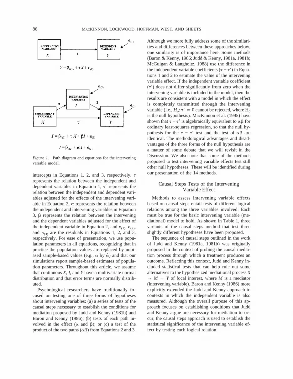
intercepts in Equations 1, 2, and 3, respectively,trepresents the relation between the independent anddependent variables in Equation 1,t8 represents therelation between the independent and dependent vari-ables adjusted for the effects of the intervening vari-able in Equation 2,a represents the relation betweenthe independent and intervening variables in Equation3, b represents the relation between the interveningand the dependent variables adjusted for the effect ofthe independent variable in Equation 2, and«(1), «(2),and «(3) are the residuals in Equations 1, 2, and 3,respectively. For ease of presentation, we use popu-lation parameters in all equations, recognizing that inpractice the population values are replaced by unbi-ased sample-based values (e.g.,a by a) and that oursimulations report sample-based estimates of popula-tion parameters. Throughout this article, we assumethat continuousX, I, andY have a multivariate normaldistribution and that error terms are normally distrib-uted.

Psychological researchers have traditionally fo-cused on testing one of three forms of hypothesesabout intervening variables: (a) a series of tests of thecausal steps necessary to establish the conditions formediation proposed by Judd and Kenny (1981b) andBaron and Kenny (1986); (b) tests of each path in-volved in the effect (a and b); or (c) a test of theproduct of the two paths (ab) from Equations 2 and 3.

Although we more fully address some of the similari-ties and differences between these approaches below,one similarity is of importance here. Some methods(Baron & Kenny, 1986; Judd & Kenny, 1981a, 1981b;McGuigan & Langholtz, 1988) use the difference inthe independent variable coefficients (t − t8) in Equa-tions 1 and 2 to estimate the value of the interveningvariable effect. If the independent variable coefficient(t8) does not differ significantly from zero when theintervening variable is included in the model, then theresults are consistent with a model in which the effectis completely transmitted through the interveningvariable (i.e.,Ho: t8 4 0 cannot be rejected, where H0

is the null hypothesis). MacKinnon et al. (1995) haveshown thatt − t8 is algebraically equivalent toab forordinary least-squares regression, so that the null hy-pothesis for thet − t8 test and the test ofab areidentical. The methodological advantages and disad-vantages of the three forms of the null hypothesis area matter of some debate that we will revisit in theDiscussion. We also note that some of the methodsproposed to test intervening variable effects test stillother null hypotheses. These will be identified duringour presentation of the 14 methods.

Causal Steps Tests of the InterveningVariable Effect

Methods to assess intervening variable effectsbased on causal steps entail tests of different logicalrelations among the three variables involved. Eachmust be true for the basic intervening variable (me-diational) model to hold. As shown in Table 1, threevariants of the causal steps method that test threeslightly different hypotheses have been proposed.

The sequence of causal steps outlined in the workof Judd and Kenny (1981a, 1981b) was originallyproposed in the context of probing the causal media-tion process through which a treatment produces anoutcome. Reflecting this context, Judd and Kenny in-cluded statistical tests that can help rule out somealternatives to the hypothesized mediational processX→ M → Y of focal interest, whereM is a mediator(intervening variable). Baron and Kenny (1986) moreexplicitly extended the Judd and Kenny approach tocontexts in which the independent variable is alsomeasured. Although the overall purpose of this ap-proach focuses on establishing conditions that Juddand Kenny argue are necessary for mediation to oc-cur, the causal steps approach is used to establish thestatistical significance of the intervening variable ef-fect by testing each logical relation.

Figure 1. Path diagram and equations for the interveningvariable model.


The series of causal steps described by Judd andKenny (1981b) and Baron and Kenny (1986) differonly slightly. Judd and Kenny (1981b, p. 605) requirethree conclusions for mediation: (a) “The treatmentaffects the outcome variable” (Ho: t 4 0), (b) “Eachvariable in the causal chain affects the variable thatfollows it in the chain, when all variables prior to it,including the treatment, are controlled” (Ho: a 4 0and Ho: b 4 0), and (c) “The treatment exerts noeffect upon the outcome when the mediating variablesare controlled” (Ho: t8 4 0). Baron and Kenny (p.1176) defined three conditions for mediation: (a)“Variations in levels of the independent variable sig-nificantly account for variations in the presumed me-diator” (Ho: a 4 0), (b) “Variations in the mediatorsignificantly account for variations in the dependentvariable” (Ho: b 4 0), and (c) “When Paths a [a] andb [b] are controlled, a previously significant relationbetween independent and dependent variables is nolonger significant, with the strongest demonstration ofmediation occurring when Path c [t8] is zero” (Ho: t84 0). Implicit in condition c is the requirement of anoverall significant relation between the independentand dependent variables (Ho: t 4 0). The centraldifference between the two variants is that Judd andKenny emphasized the importance of demonstratingcomplete mediation, which would occur when the hy-potheses thatt8 4 0 cannot be rejected. Baron andKenny argued that models in which there is only par-tial mediation (i.e., |t8| < |t|) rather than completemediation are acceptable. They pointed out that suchmodels are more realistic in most social science re-search because a single mediator cannot be expectedto completely explain the relation between an inde-pendent and a dependent variable.

A third variant of the causal steps approach has alsobeen used by some researchers (Cohen & Cohen,1983, p. 366). In this variant, researchers claim evi-dence for intervening variable effects when separatetests of each path in the intervening variable effect (aandb) are jointly significant (Ho: a 4 0 andHo: b 40). This method simultaneously tests whether the in-dependent variable is related to the intervening vari-able and whether the intervening variable is related tothe dependent variable. A similar test was also out-lined by Allison (1995). Kenny, Kashy, and Bolger(1998) restated the Judd and Kenny causal steps butnoted that the tests ofa andb are the essential testsfor establishing mediation. This method provides themost direct test of the simultaneous null hypothesisthat patha and pathb are both equal to 0. However,

this method provides no test of either theab productor the overallX → Y relation.

In summary, the widely used Judd and Kenny(1981b) and Baron and Kenny (1986) variants of thecausal steps approach clearly specify the conceptuallinks between each hypothesized causal relation andthe statistical tests of these links. However, as de-scribed in more depth in the Discussion, these twoapproaches probe, but do not provide, the full set ofnecessary conditions for the strong inference of acausal effect of the independent variable on the de-pendent variable through the intervening variable,even when subjects are randomly assigned to the lev-els of the independent variable in a randomized ex-periment (Baron & Kenny, 1986; Holland, 1988;MacKinnon, 1994). Because the overall purpose ofthe causal steps methods was to establish conditionsfor mediation rather than a statistical test of the indi-rect effect ofX on Y throughI (e.g.,ab), they haveseveral limitations. The causal steps methods do notprovide a joint test of the three conditions (conditionsa, b, and c), a direct estimate of the size of the indirecteffect of X on Y, or standard errors to construct con-fidence limits, although the standard error of the in-direct effect ofX on Y is given in the descriptions ofthe causal steps method (Baron & Kenny, 1986;Kenny et al., 1998). In addition, it is difficult to ex-tend the causal steps method to models incorporatingmultiple intervening variables and to evaluate each ofthe intervening variable effects separately in a modelwith more than one intervening variable (e.g., Mac-Kinnon, 2000; West & Aiken, 1997). Finally, the re-quirement that there has to be a significant relationbetween the independent and dependent variables ex-cludes many “inconsistent” intervening variable mod-els in which the indirect effect (ab) and direct effect(t8) have opposite signs and may cancel out (Mac-Kinnon, Krull, & Lockwood, 2000).

Difference in Coefficients Tests of theIntervening Variable Effect

Intervening variable effects can be assessed bycomparing the relation between the independent vari-able and the dependent variable before and after ad-justment for the intervening variable. Several differ-ent pairs of coefficients can be compared, includingthe regression coefficients (t − t8) described aboveand correlation coefficients,rXY − rXY.I, although, asdescribed below, the method based on correlationsdiffers from other tests of the intervening variable


effect. In the above expression,rXY is the correlationbetween the independent variable and the dependentvariable andrXY.I is the partial correlation between theindependent variable and the dependent variable par-tialled for the intervening variable. Each of the vari-ants of the difference in coefficients tests is summa-rized in the middle part of Table 1. Readers shouldnote that these procedures test a diverse set of nullhypotheses about intervening variables.

Freedman and Schatzkin (1992) developed amethod to study binary health measures that can beextended to the difference between the adjusted andunadjusted regression coefficients (Ho: t − t8 4 0).Freedman and Schatzkin derived the correlation be-tweent andt8 that can be used in an equation for thestandard error based on the variance and covariance ofthe adjusted and unadjusted regression coefficients:

sFreedman–Schatzkin= =st2 + st8

2 − 2stst8=1 − rXI2 .

(4)

In this equation,rXI is equal to the correlation be-tween the independent variable and the interveningvariable,st is the standard error oft, andst8 is thestandard error oft8. The estimate oft − t8 is dividedby the standard error in Equation 4 and this value iscompared to thet distribution for a test of signifi-cance.

McGuigan and Langholtz (1988) also derived thestandard error of the difference between these tworegression coefficients (Ho: t − t8 4 0) for standard-ized variables. They found the standard error of thet − t8 method to be equal to

sMcGuigan–Langholtz= =st2 + st8

2 − 2~rtt8stst8!. (5)

The covariance betweent and t8 (rtt8stst8), appli-cable for either standardized or unstandardized vari-ables, is the mean square error (sMSE) from Equation2 divided by the product of sample size and the vari-ance ofX. The difference between the two regressioncoefficients (t − t8) is then divided by the standarderror in Equation 5 and this value is compared to thet distribution for a significance test. MacKinnon et al.(1995) found that the original formula for the standarderror proposed by McGuigan and Langholtz was in-accurate for a binary (i.e., unstandardized) indepen-dent variable. On the basis of their derivation, weobtained the corrected formula given above that isaccurate for standardized or unstandardized indepen-dent variables.

Another estimate of the standard error oft − t8 was

developed from a test of collapsibility (Clogg, Pet-kova, & Shihadeh, 1992). Clogg et al. extended thenotion of collapsibility in categorical data analysis tocontinuous measures. Collapsibility tests whether it isappropriate to ignore or collapse across a third vari-able when examining the relation between two vari-ables. In this case, collapsibility is a test of whether anintervening variable significantly changes the relationbetween two variables. As shown below, the standarderror of t − t8 in Clogg et al. (1992) is equal to theabsolute value of the correlation between the indepen-dent variable and the intervening variable times thestandard error oft8:

sClogg et al.=sMSE?rXI?

=sX@n~1 − rXI2 !#

= ?rXI?st8. (6)

Furthermore, Clogg et al. (1992) showed that the sta-tistical test oft − t8 divided by its standard error isequivalent to testing the null hypothesis,Ho: b 4 0.This indicates that a significance test of the interven-ing variable effect can be obtained simply by testingthe significance ofb or by dividing t − t8 by thestandard error in Equation 6 and comparing the valueto the t distribution. Although Clogg et al.’s (1992)approach testsHo: t − t8 4 0, Allison (1995) andClogg, Petkova, and Cheng (1995) demonstrate thatthe derivation assumes that bothX and I are fixed,which is unlikely for a test of an intervening variable.

A method based on correlations (Ho: rXY − rXY.I 40) compares the correlation betweenX andY beforeand after it is adjusted forI as shown in Equation 7.The difference between the simple and partial corre-lations is the measure of how much the interveningvariable changes the simple correlation, whererIY isthe correlation between the intervening variable andthe dependent variable. The null hypothesis for thistest is distinctly different from any of the three formsthat have been used in psychology (see p. 86). Asnoted by a reviewer, there are situations where thedifference between the simple and partial correlationis nonzero, yet the correlation between the interveningvariable and the dependent variable partialled for theindependent variable is zero. In these situations, themethod indicates an intervening variable effect whenthere is not evidence that the intervening variable isrelated to the dependent variable. The problem occursbecause of constraints on the range of the partial cor-relation:

rdifference= rXY −rXY − rIYrXI

=~1 − rIY2 !~1 − rXI

2 !. (7)


Olkin and Finn (1995) used the multivariate deltamethod to find the large sample standard error of thedifference between a simple correlation and the samecorrelation partialled for a third variable. The differ-ence between the simple and partial correlation is thendivided by the calculated standard error and comparedto the standard normal distribution to test for an in-tervening variable effect. The large sample solutionsfor the variances and covariances among the correla-tions are shown in Appendix A and the vector ofpartial derivatives shown in Equation 8 is used to findthe standard error of the difference. There is a typo-graphical error in this formula in Olkin and Finn (p.160) that is corrected in Equation 8. The partial de-rivatives are

F rIY − rXIrXY

~1 − rIY2 !1/2~1 − rXI

2 !3/2,

1 −1

=~1 − rIY2 !~1 − rXI

2 !,

rXI − rXYrIY

~1 − rXI2 !1/2~1 − rIY

2 !3/2G.

(8)

For the two tests of intervening variable effects (theother test is described below) where standard errorsare derived using the multivariate delta method, thepartial derivatives are presented in the text rather thanshowing the entire formula for the standard error,which is long. A summary of the multivariate deltamethod is shown in Appendix A. An SAS (Version6.12) program to compute the standard errors isshown in Appendix B.

In summary, each difference in coefficients methodprovides an estimate of some intervening variable ef-fect and its standard error. Depending on the proce-dure, the null hypothesis may or may not resembleones commonly proposed in psychology. The null hy-pothesis of the Clogg et al. (1992) test assumes fixedX andI, which is not likely for intervening variables.The difference between the simple and partial corre-lation represents a unique test of the intervening vari-able effect because there are situations where thereappears to be no relation between the intervening anddependent variable, yet the method suggests that anintervening variable effect exists. An additional draw-back of this general approach is that the underlyingmodel for some tests, such as the difference betweensimple and partial correlation, is based on nondirec-tional correlations that do not directly follow but areimplied by the path model in Figure 1. The differencein coefficients methods also does not provide a clearframework for generalizing the tests to estimate ap-

propriate coefficients and test significance of their dif-ference in models with more than one interveningvariable.

Product of Coefficients Tests for theIntervening Variable Effect

The third general approach is to test the signifi-cance of the intervening variable effect by dividingthe estimate of the intervening variable effect,ab, byits standard error and comparing this value to a stan-dard normal distribution. There are several variants ofthe standard error formula based on different assump-tions and order of derivatives in the approximations.These variants are summarized in the bottom part ofTable 1.

The most commonly used standard error is the ap-proximate formula derived by Sobel (1982) using themultivariate delta method based on a first order Tay-lor series approximation:

sab first = =a2sb2 + b2sa

2. (9)

The intervening variable effect is divided by the stan-dard error in Equation 9, which is then compared to astandard normal distribution to test for significance(Ho: ab 4 0). This standard error formula is used incovariance structure programs such as EQS (Bentler,1997) and LISREL (Jo¨reskog & So¨rbom, 1993).

The exact standard error based on first and secondorder Taylor series approximation (Aroian, 1944) ofthe product ofa andb is

sab second= =a2sb2 + b2sa

2 + sa2sb

2. (10)

The intervening variable effect is divided by the stan-dard error in Equation 10, which is then compared toa standard normal distribution to test for significance(Ho: ab 4 0). Equation 9 excludes the product of thetwo variances, which is part of the exact standarderror in Equation 10, although that term is typicallyvery small.

Goodman (1960; Sampson & Breunig, 1971) de-rived the unbiased variance of the product of twonormal variables, which subtracts the product of vari-ances, giving

sab unbiased= =a2sb2 + b2sa

2 − sa2sb

2. (11)

A test of the intervening variable effect can be ob-tained by dividingab by the standard error in Equa-tion 11, which is then compared to a standard normaldistribution to test for significance.


MacKinnon, Lockwood, and Hoffman (1998)showed evidence that theab/sab methods to test thesignificance of the intervening variable effect havelow power because the distribution of the product ofregression coefficientsa and b is not normally dis-tributed, but rather is often asymmetric with high kur-tosis. Under the conditions of multivariate normalityof X, I, andY, the two paths represented bya andbin Figure 1 are independent (MacKinnon, Warsi, &Dwyer, 1995; Sobel, 1982). On the basis of the sta-tistical theory of the products of random variables(Craig, 1936; Meeker, Cornwell, & Aroian, 1981;Springer & Thompson, 1966), MacKinnon and col-leagues (MacKinnon et al., 1998; MacKinnon &Lockwood, 2001) proposed three alternative variants(presented below) that theoretically should be moreaccurate: (a) empirical distribution ofab/sab (Ho:ab/sab 4 0), (b) distribution of the product of twostandard normal variables,zazb (Ho: zazb 4 0), and(c) asymmetric confidence limits for the distributionof the product,ab (Ho: ab 4 0).

In the first variant, MacKinnon et al. (1998) con-ducted extensive simulations to estimate the empiricalsampling distribution ofab for a wide range of valuesof a andb. On the basis of these empirical samplingdistributions, critical values for different significancelevels were determined. These tables of critical valuesare available at http://www.public.asu.edu/∼davidpm/ripl/methods.htm. For example, the empirical criticalvalue is .97 for the .05 significance level rather than1.96 for the standard normal test ofab 4 0. Wedesignate this test statistic by z8 because it uses adifferent distribution than the normal distribution.

A second variant of the test of the intervening vari-able effect involves the distribution of the product oftwo z statistics—one for thea parameter,za 4 a/sa,and another for theb parameter,zb 4 b/sb. If a andb are assumed to be normal, thezazb term can bedirectly tested for significance using critical valuesbased on the theoretical distribution of the product oftwo normal random variables,P 4 zazb. This testinvolves converting both thea and theb paths tozscores, multiplying thezs, and using a critical valuebased on the distribution of the product of randomvariables, P4 zazb, from Craig (1936; see alsoMeeker et al., 1981; Springer & Thompson, 1966) todetermine significance. For example, the critical valueto testab 4 0 for the .05 significance level for the P4 zazb distribution is 2.18, rather than 1.96 for thenormal distribution.

A third variant constructs asymmetric confidence

limits to accommodate the nonnormal distribution ofthe intervening variable effect based on the distribu-tion of the product of random variables. Again, twozstatistics are computed,za 4 a/sa and zb 4 b/sb.These values are then used to find critical values forthe product of two random variables from the tables inMeeker et al. (1981) to find lower and upper signifi-cance levels. Those values are used to compute lowerand upper confidence limits using the formula CL4ab± (critical value) sab. If the confidence intervaldoes not include zero, the intervening variable effectis significant.

Bobko and Rieck (1980) examined interveningvariable effects in path analysis using regression co-efficients from the analysis of standardized variables(Ho: asbs 4 0, whereas andbs are from regressionanalysis of standardized variables). These researchersused the multivariate delta method to find an estimateof the variance of the intervening variable effect forstandardized variables, based on the product of thecorrelation betweenX andI and the partial regressioncoefficient relatingI and Y, controlling for X. Thefunction of the product of these terms is

rproduct=rXI~rIY − rXYrXI!

1 − rXI2 . (12)

The partial derivatives of this function given in Bobkoand Rieck (1980) are

FrXI2 rIY + rIY − 2rXIrXY

~1 − rXI2 !2

,−rXI

2

1 − rXI2 ,

rXI

1 − rXI2 G. (13)

The variance–covariance matrix of the correlation co-efficients is pre- and postmultiplied by the vector ofpartial derivatives to calculate a standard error thatcan be used to test the significance of the interveningvariable effect.

The product of coefficients methods provide esti-mates of the intervening variable effect and the stan-dard error of the intervening variable effect. In addi-tion, the underlying model follows directly from pathanalysis wherein the intervening variable effect is theproduct of coefficients hypothesized to measurecausal relations. This logic directly extends to modelsincorporating multiple intervening variables (Bollen,1987). However, as is presented below, two problemsoccur in conducting these tests. First, the samplingdistribution of these tests does not follow the normaldistribution as is typically assumed. Second, the formof the null hypothesis that is tested is complex.


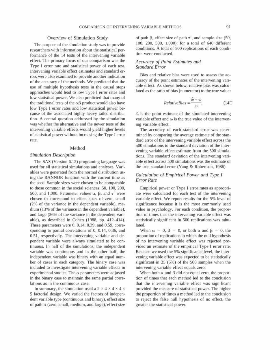
Overview of Simulation StudyThe purpose of the simulation study was to provide

researchers with information about the statistical per-formance of the 14 tests of the intervening variableeffect. The primary focus of our comparison was theType I error rate and statistical power of each test.Intervening variable effect estimates and standard er-rors were also examined to provide another indicationof the accuracy of the methods. We predicted that theuse of multiple hypothesis tests in the causal stepsapproaches would lead to low Type I error rates andlow statistical power. We also predicted that many ofthe traditional tests of theab product would also havelow Type I error rates and low statistical power be-cause of the associated highly heavy tailed distribu-tion. A central question addressed by the simulationwas whether the alternative and the newer tests of theintervening variable effects would yield higher levelsof statistical power without increasing the Type I errorrate.

MethodSimulation Description

The SAS (Version 6.12) programing language wasused for all statistical simulations and analyses. Vari-ables were generated from the normal distribution us-ing the RANNOR function with the current time asthe seed. Sample sizes were chosen to be comparableto those common in the social sciences: 50, 100, 200,500, and 1,000. Parameter valuesa, b, andt8 werechosen to correspond to effect sizes of zero, small(2% of the variance in the dependent variable), me-dium (13% of the variance in the dependent variable),and large (26% of the variance in the dependent vari-able), as described in Cohen (1988, pp. 412–414).These parameters were 0, 0.14, 0.39, and 0.59, corre-sponding to partial correlations of 0, 0.14, 0.36, and0.51, respectively. The intervening variable and de-pendent variable were always simulated to be con-tinuous. In half of the simulations, the independentvariable was continuous and in the other half, theindependent variable was binary with an equal num-ber of cases in each category. The binary case wasincluded to investigate intervening variable effects inexperimental studies. Thea parameters were adjustedin the binary case to maintain the same partial corre-lations as in the continuous case.

In summary, the simulation used a 2 × 4 × 4 × 4 ×5 factorial design. We varied the factors of indepen-dent variable type (continuous and binary), effect sizeof patha (zero, small, medium, and large), effect size

of pathb, effect size of patht8, and sample size (50,100, 200, 500, 1,000), for a total of 640 differentconditions. A total of 500 replications of each condi-tion were conducted.

Accuracy of Point Estimates andStandard Error

Bias and relative bias were used to assess the ac-curacy of the point estimates of the intervening vari-able effect. As shown below, relative bias was calcu-lated as the ratio of bias (numerator) to the true value:

RelativeBias=v − v

v, (14)

v is the point estimate of the simulated interveningvariable effect andv is the true value of the interven-ing variable effect.

The accuracy of each standard error was deter-mined by comparing the average estimate of the stan-dard error of the intervening variable effect across the500 simulations to the standard deviation of the inter-vening variable effect estimate from the 500 simula-tions. The standard deviation of the intervening vari-able effect across 500 simulations was the estimate ofthe true standard error (Yang & Robertson, 1986).

Calculation of Empirical Power and Type IError Rate

Empirical power or Type I error rates as appropri-ate were calculated for each test of the interveningvariable effect. We report results for the 5% level ofsignificance because it is the most commonly usedvalue in psychology. For each condition, the propor-tion of times that the intervening variable effect wasstatistically significant in 500 replications was tabu-lated.

When a 4 0, b 4 0, or botha and b 4 0, theproportion of replications in which the null hypothesisof no intervening variable effect was rejected pro-vided an estimate of the empirical Type I error rate.Because we used the 5% significance level, the inter-vening variable effect was expected to be statisticallysignificant in 25 (5%) of the 500 samples when theintervening variable effect equals zero.

When botha andb did not equal zero, the propor-tion of times that each method led to the conclusionthat the intervening variable effect was significantprovided the measure of statistical power. The higherthe proportion of times a method led to the conclusionto reject the false null hypothesis of no effect, thegreater the statistical power.


The 14 procedures reference different statisticaldistributions. In each case, we used the critical valuesfrom the reference distribution for the test. For thosetests based on asymptotic methods, we used 1.96 fromthe normal distribution. For the z8 4 ab/sab test weused critical values described in MacKinnon et al.(1998) indicated by z8, and for the test for P4 zazb

we used critical values from Craig (1936) indicated byP. The upper and lower confidence limits for theasymmetric confidence limits test were taken from thetabled values in Meeker et al. (1981). The causal stepstests involve multiple hypothesis tests so there is nosingle reference distribution. For these tests, the in-tervening variable effect was considered significant ifeach of the steps was satisfied.

Results

In general, the simulation results for the binary casedid not differ from those of the continuous indepen-dent variable case. Consequently, we present only theresults for the continuous independent variable below.

Intervening Variable Effect Estimates

As found in other studies, most estimates of theintervening variable effect had minimal bias with theexception ofzazb, which had substantial bias becausethe point estimates of this quantity were much largerthan other point estimates of the intervening variableeffect. Only thezazb test had bias greater than .01,even at a sample size of 50. Relative bias decreased assample size and effect size increased for all estimates,including zazb.

Accuracy of Standard Errors

The accuracy of the formulas for standard errors ofthe intervening variable effect was examined by com-paring a measure of the true standard error (the stan-dard deviation of the intervening variable effect esti-mate across the 500 replications in each condition) tothe average standard error estimate as shown in Table2. For theab 4 t − t8 estimate, all standard errorswere generally accurate except for the Freedman andSchatzkin (1992) and the Clogg et al. (1992) standarderror estimates, which were much smaller than thetrue values for all conditions. Goodman’s (1960) un-biased method frequently yielded undefined (imagi-nary) standard errors. These findings raise serious is-sues about the use of this approach. For example,Goodman’s unbiased standard error was undefinedapproximately 40% of the time when the true effectsize was zero and 10% of the time when the effect sizewas small and sample size was 50. We did not include

cases that resulted in undefined standard errors in thecomputation of the mean standard error in Table 2.

As shown in Table 3, the standard errors for theproduct of regression coefficients for standardized

Table 2Comparison of Estimates of the Standard Error oft − t8= ab

Effect size

Sample size

50 100 200 500 1,000

Standard deviation fort − t8 4 abZero .0224 .0121 .0049 .0022 .0009Small .0376 .0214 .0162 .0089 .0062Medium .0855 .0549 .0386 .0251 .0184Large .1236 .0857 .0585 .0366 .0257

Freedman & Schatzkin (1992)Zero .0171 .0083 .0041 .0016 .0008Small .0238 .0154 .0107 .0062 .0045Medium .0598 .0402 .0282 .0178 .0126Large .0903 .0622 .0444 .0274 .0193

McGuigan & Langholtz (1988)Zero .0342 .0169 .0082 .0033 .0016Small .0431 .0260 .0165 .0093 .0065Medium .0867 .0577 .0400 .0250 .0175Large .1252 .0861 .0603 .0374 .0264

Clogg et al. (1992)Zero .0168 .0083 .0041 .0016 .0008Small .0233 .0152 .0107 .0062 .0045Medium .0579 .0392 .0276 .0175 .0123Large .0859 .0595 .0428 .0264 .0186

Sobel (1982) first orderZero .0264 .0129 .0062 .0025 .0012Small .0371 .0236 .0156 .0090 .0064Medium .0841 .0568 .0397 .0249 .0175Large .1235 .0855 .0601 .0374 .0264

Aroian (1944) second orderZero .0348 .0170 .0082 .0033 .0016Small .0435 .0261 .0165 .0093 .0065Medium .0869 .0577 .0400 .0249 .0175Large .1253 .0861 .0603 .0374 .0264

Goodman (1960) UnbiasedZero .0257 .0135 .0060 .0026 .0012Small .0368 .0224 .0148 .0088 .0063Medium .0814 .0558 .0393 .0248 .0175Large .1217 .0848 .0599 .0373 .0264

Note. The measure of the true standard error is the standard de-viation of t − t8 4 ab. The Goodman (1960) standard error wasundefined (negative variance) for the zero effect, 185, 203, 195,208, and 190 times for samples sizes of 50, 100, 200, 500, and1,000, respectively. The Goodman standard error was undefined forthe small effect size 106, 38, and 5 times for sample sizes of 50,100, and 200, respectively, and undefined 1 time for medium effectand a sample size of 50.


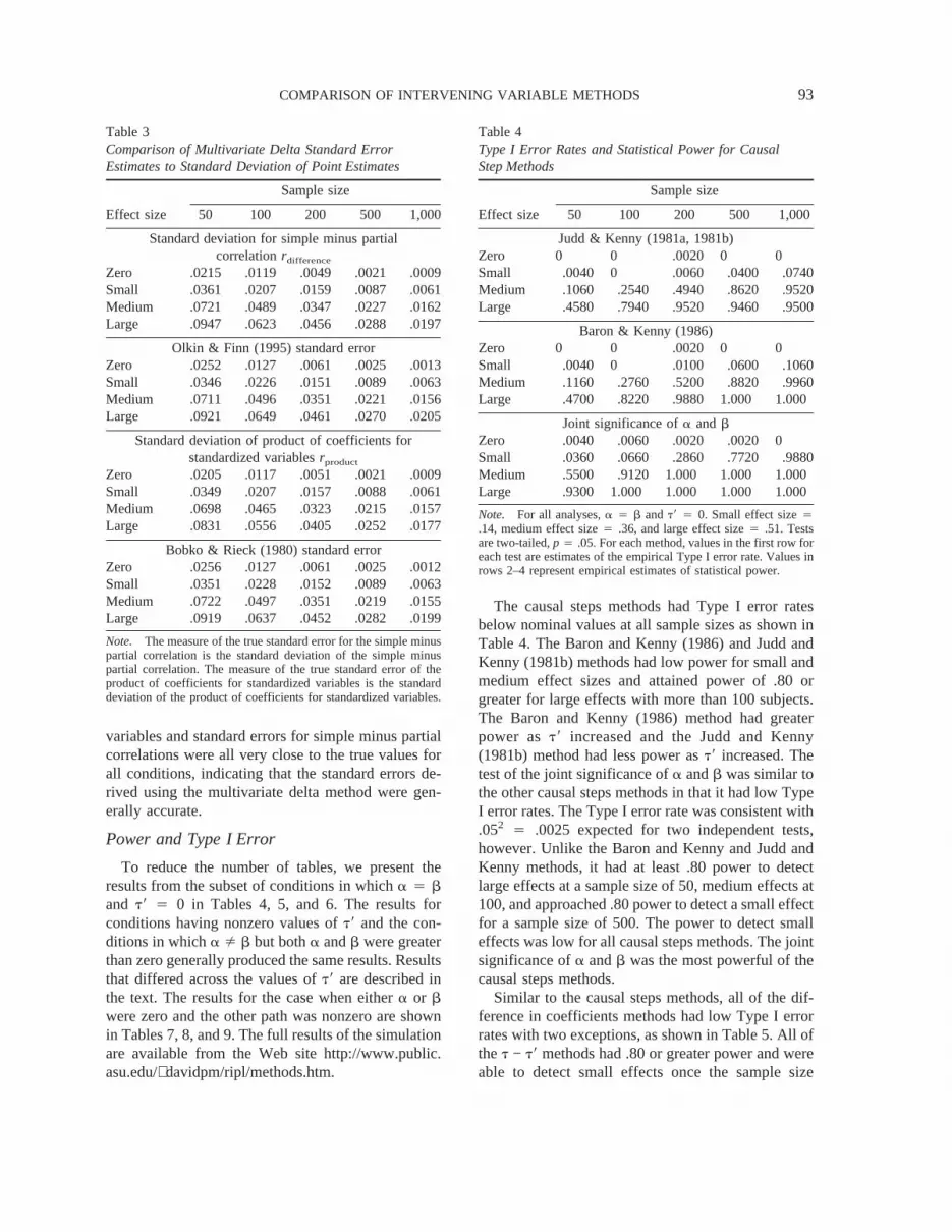
variables and standard errors for simple minus partialcorrelations were all very close to the true values forall conditions, indicating that the standard errors de-rived using the multivariate delta method were gen-erally accurate.

Power and Type I Error

To reduce the number of tables, we present theresults from the subset of conditions in whicha 4 band t8 4 0 in Tables 4, 5, and 6. The results forconditions having nonzero values oft8 and the con-ditions in whicha Þ b but botha andb were greaterthan zero generally produced the same results. Resultsthat differed across the values oft8 are described inthe text. The results for the case when eithera or bwere zero and the other path was nonzero are shownin Tables 7, 8, and 9. The full results of the simulationare available from the Web site http://www.public.asu.edu/∼davidpm/ripl/methods.htm.

The causal steps methods had Type I error ratesbelow nominal values at all sample sizes as shown inTable 4. The Baron and Kenny (1986) and Judd andKenny (1981b) methods had low power for small andmedium effect sizes and attained power of .80 orgreater for large effects with more than 100 subjects.The Baron and Kenny (1986) method had greaterpower ast8 increased and the Judd and Kenny(1981b) method had less power ast8 increased. Thetest of the joint significance ofa andb was similar tothe other causal steps methods in that it had low TypeI error rates. The Type I error rate was consistent with.052 4 .0025 expected for two independent tests,however. Unlike the Baron and Kenny and Judd andKenny methods, it had at least .80 power to detectlarge effects at a sample size of 50, medium effects at100, and approached .80 power to detect a small effectfor a sample size of 500. The power to detect smalleffects was low for all causal steps methods. The jointsignificance ofa andb was the most powerful of thecausal steps methods.

Similar to the causal steps methods, all of the dif-ference in coefficients methods had low Type I errorrates with two exceptions, as shown in Table 5. All ofthet − t8 methods had .80 or greater power and wereable to detect small effects once the sample size

Table 3Comparison of Multivariate Delta Standard ErrorEstimates to Standard Deviation of Point Estimates

Effect size

Sample size

50 100 200 500 1,000

Standard deviation for simple minus partialcorrelationrdifference

Zero .0215 .0119 .0049 .0021 .0009Small .0361 .0207 .0159 .0087 .0061Medium .0721 .0489 .0347 .0227 .0162Large .0947 .0623 .0456 .0288 .0197

Olkin & Finn (1995) standard errorZero .0252 .0127 .0061 .0025 .0013Small .0346 .0226 .0151 .0089 .0063Medium .0711 .0496 .0351 .0221 .0156Large .0921 .0649 .0461 .0270 .0205

Standard deviation of product of coefficients forstandardized variablesrproduct

Zero .0205 .0117 .0051 .0021 .0009Small .0349 .0207 .0157 .0088 .0061Medium .0698 .0465 .0323 .0215 .0157Large .0831 .0556 .0405 .0252 .0177

Bobko & Rieck (1980) standard errorZero .0256 .0127 .0061 .0025 .0012Small .0351 .0228 .0152 .0089 .0063Medium .0722 .0497 .0351 .0219 .0155Large .0919 .0637 .0452 .0282 .0199

Note. The measure of the true standard error for the simple minuspartial correlation is the standard deviation of the simple minuspartial correlation. The measure of the true standard error of theproduct of coefficients for standardized variables is the standarddeviation of the product of coefficients for standardized variables.

Table 4Type I Error Rates and Statistical Power for CausalStep Methods

Effect size

Sample size

50 100 200 500 1,000

Judd & Kenny (1981a, 1981b)Zero 0 0 .0020 0 0Small .0040 0 .0060 .0400 .0740Medium .1060 .2540 .4940 .8620 .9520Large .4580 .7940 .9520 .9460 .9500

Baron & Kenny (1986)Zero 0 0 .0020 0 0Small .0040 0 .0100 .0600 .1060Medium .1160 .2760 .5200 .8820 .9960Large .4700 .8220 .9880 1.000 1.000

Joint significance ofa andbZero .0040 .0060 .0020 .0020 0Small .0360 .0660 .2860 .7720 .9880Medium .5500 .9120 1.000 1.000 1.000Large .9300 1.000 1.000 1.000 1.000

Note. For all analyses,a 4 b andt8 4 0. Small effect size4.14, medium effect size4 .36, and large effect size4 .51. Testsare two-tailed,p 4 .05. For each method, values in the first row foreach test are estimates of the empirical Type I error rate. Values inrows 2–4 represent empirical estimates of statistical power.


reached 1,000, medium effects at 100, and large ef-fects at a sample size of 50. Only the Clogg et al.(1992) and Freedman and Schatzkin (1992) methodshad accurate Type I error rates (i.e., close to .05) andgreater than .80 power to detect a small, medium, andlarge effect at sample sizes of 500, 100, and 50, re-spectively. Even though the standard errors fromthese methods appeared to underestimate the truestandard error, they had the most accurate Type I errorrates and higher statistical power. This pattern of re-sults suggests that a standard error that is too smallmay be partially compensating for the higher criticalvalues associated with the nonnormal distribution ofthe intervening variable effect.

Like most of the previous methods, the product ofcoefficients methods generally had Type I error ratesbelow .05 and adequate power to detect small, me-dium, and large effects for sample sizes of 1,000, 100,and 50 respectively. The distribution of products test,P 4 zazb, and the distribution of z8 4 ab/sab testhad accurate Type I error rates and the most power of

all tests. These results are presented in Table 6. At asample size of 50, the two distribution methods hadpower of above .80 to detect medium and large effectsand detected small effects with .80 power at a sample

Table 5Type I Error Rates and Statistical Power for Differencein Coefficients Methods

Effect size

Sample size

50 100 200 500 1,000

t − t8 (Freedman & Schatzkin, 1992)Zero .0160 .0440 .0180 .0520 .0500Small .1240 .2280 .5060 .8900 .9920Medium .7100 .9560 1.000 1.000 1.000Large .9560 1.000 1.000 1.000 1.000

t − t8 (McGuigan & Langholtz, 1988)Zero 0 0 0 0 0Small .0060 .0060 .0920 .5260 .9740Medium .3380 .8540 1.000 1.000 1.000Large .8920 1.000 1.000 1.000 1.000

t − t8 (Clogg et al., 1992)Zero .0320 .0660 .0320 .0620 .0540Small .1780 .2840 .5100 .8920 .9920Medium .7320 .9560 1.000 1.000 1.000Large .9580 1.000 1.000 1.000 1.000

Simple minus partial correlation (Olkin & Finn, 1995)Zero .0020 0 .0020 0 0Small .0100 .0120 .1260 .5780 .9800Medium .4340 .8920 1.000 1.000 1.000Large .9380 1.000 1.000 1.000 1.000


Table 6Type I Error Rates and Statistical Power for Product ofCoefficients Methods

Effect size

Sample size

50 100 200 500 1,000

First-order test (Sobel, 1982)Zero 0 0 .0020 0 0Small .0060 .0100 .1220 .5620 .9760Medium .3600 .8620 1.000 1.000 1.000Large .9020 1.000 1.000 1.000 1.000

Second-order test (Aroian, 1944)Zero 0 0 0 0 0Small .0060 .0060 .0920 .5260 .9740Medium .3320 .8540 1.000 1.000 1.000Large .8920 1.000 1.000 1.000 1.000

Unbiased test (Goodman, 1960)Zero .0160 .0040 .0140 .0020 .0100Small .0080 .0200 .1420 .6200 .9820Medium .3900 .8700 1.000 1.000 1.000Large .9120 1.000 1.000 1.000 1.000

Distribution of products test P4 zazb

(MacKinnon et al., 1998)Zero .0620 .0760 .0420 .0660 .0400Small .2220 .3960 .7180 .9740 1.000Medium .9180 .9960 1.000 1.000 1.000Large 1.000 1.000 1.000 1.000 1.000

Distribution of ab/sab (MacKinnon et al., 1998)Zero .0560 .0680 .0400 .0600 .0420Small .2060 .3600 .6920 .9580 .9960Medium .9040 .9960 1.000 1.000 1.000Large .9980 1.000 1.000 1.000 1.000

Asymmetric distribution of products test(MacKinnon & Lockwood, 2001)

Zero .0040 .0040 .0020 0 0Small .0300 .0620 .2740 .7600 .9880Medium .5540 .9200 1.000 1.000 1.000Large .9400 1.000 1.000 1.000 1.000

Product of coefficients for standardized variables(Bobko & Rieck, 1980)

Zero .0020 0 .0020 0 0Small .0080 .0160 .1300 .5700 .9780Medium .4200 .8760 1.000 1.000 1.000Large .9200 1.000 1.000 1.000 1.000



size of 500. The asymmetric confidence limits methodalso had Type I error rates that were too low but hadmore power than the other product of coefficientmethods.

Overall, the two distribution methods, P4 zazb,andz8 4 ab/sab, the Clogg et al. (1992), and Freed-man and Schatzkin (1992) methods performed thebest of all of the methods tested in terms of the mostaccurate Type I error rates and the greatest statisticalpower. However, recall that the Clogg et al. (1992)method assumes fixed effects forX and I (equivalentto a test of the significance ofb) so that it may not bea good test on conceptual grounds. The similar per-formance of the Freedman and Schatzkin test suggeststhat this method is also based on fixed effects forXandI. These methods were superior whenever botha4 0 andb 4 0 and for all combinations ofa andbvalues as long as both parameters were nonzero. Forcases when eithera 4 0 andb was nonzero ora wasnonzero andb 4 0, these methods were not the mostaccurate (see Tables 7, 8, and 9). Thea path could benonsignificant and quite small, yet these methodswould suggest a statistically significant intervening

variable effect when theb path was a medium or largeeffect. In the case wherea 4 0 and theb effect waslarge, these methods yielded Type I error rates thatwere too high, although the distribution methods, P4zazb and z8 4 ab/sab, performed better than the dif-ference in coefficients methods. Whena was a largeeffect andb 4 0, the Clogg et al. (1992) and Freed-man and Schatzkin methods worked well and the dis-tribution of products methods did not. The joint sig-nificance test ofa andb, the asymmetric confidencelimits test, and the tests based on dividing theabintervening variable effect by the standard error ofabhad more accurate standard errors in the case whereone of thea andb parameters was equal to zero.

Discussion

In our discussion, we initially focus on the statisti-cal performance of each of the 14 tests of the effect ofthe intervening variable effect that were considered.We then focus on statistical recommendations andmore general conceptual and practical issues associ-ated with the choice of a test of an intervening vari-able effect.

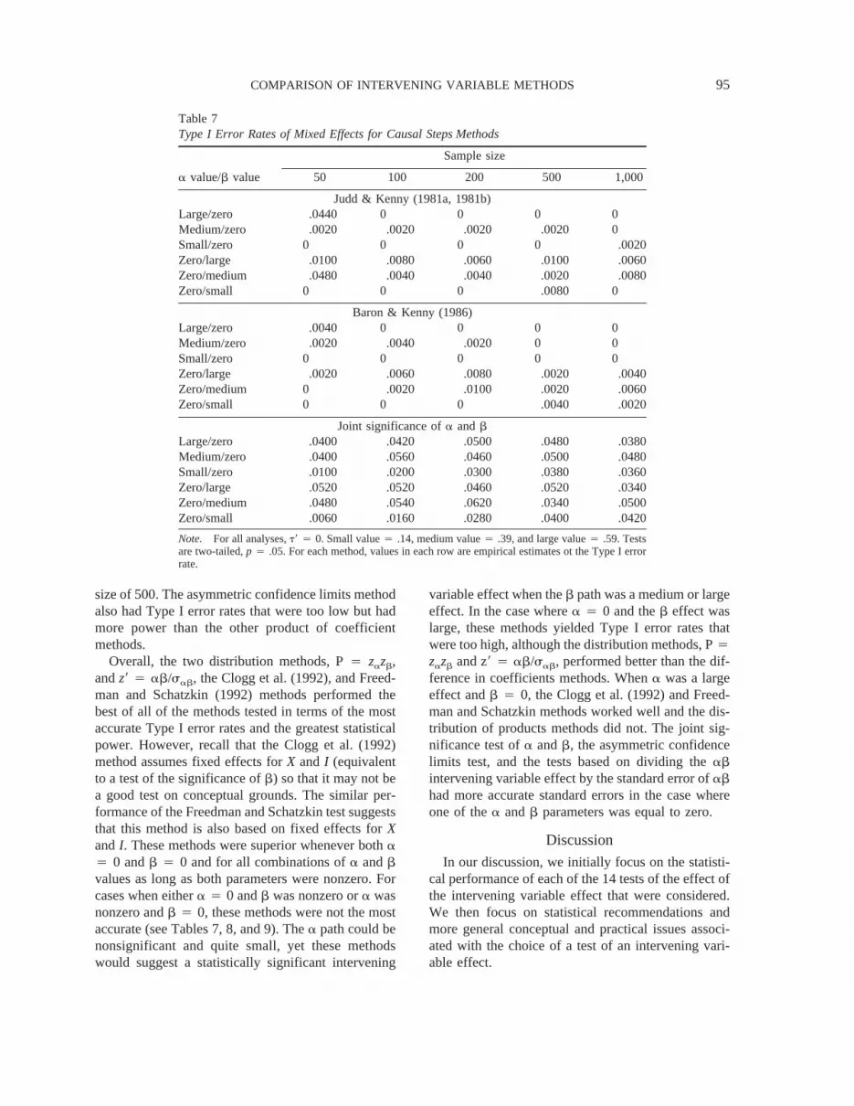
Table 7Type I Error Rates of Mixed Effects for Causal Steps Methods

a value/b value

Sample size

50 100 200 500 1,000

Judd & Kenny (1981a, 1981b)Large/zero .0440 0 0 0 0Medium/zero .0020 .0020 .0020 .0020 0Small/zero 0 0 0 0 .0020Zero/large .0100 .0080 .0060 .0100 .0060Zero/medium .0480 .0040 .0040 .0020 .0080Zero/small 0 0 0 .0080 0

Baron & Kenny (1986)Large/zero .0040 0 0 0 0Medium/zero .0020 .0040 .0020 0 0Small/zero 0 0 0 0 0Zero/large .0020 .0060 .0080 .0020 .0040Zero/medium 0 .0020 .0100 .0020 .0060Zero/small 0 0 0 .0040 .0020

Joint significance ofa andbLarge/zero .0400 .0420 .0500 .0480 .0380Medium/zero .0400 .0560 .0460 .0500 .0480Small/zero .0100 .0200 .0300 .0380 .0360Zero/large .0520 .0520 .0460 .0520 .0340Zero/medium .0480 .0540 .0620 .0340 .0500Zero/small .0060 .0160 .0280 .0400 .0420

Note. For all analyses,t8 4 0. Small value4 .14, medium value4 .39, and large value4 .59. Testsare two-tailed,p 4 .05. For each method, values in each row are empirical estimates ot the Type I errorrate.


Statistical Performance

The most widely used methods proposed by Juddand Kenny (1981b) and Baron and Kenny (1986) haveType I error rates that are too low in all the simulationconditions and have very low power, unless the effector sample size is large. For example, these methodshave only .106 empirical power to detect small effectsat a sample size of 1,000 and only .49 power to detectmoderate effects at a sample size of 200. Overall, thestep requiring a significant total effect ofX on Y (t)led to the most Type II errors. As a result, the Baronand Kenny (1986) causal steps method had fewerType II errors as the value oft8 increased. The Juddand Kenny (1981b) causal steps method had moreType II errors ast8 increased because of the require-

ment thatt8 not be statistically significant. Studiesthat use the causal steps methods described by Kennyand colleagues are the most likely to miss real effectsbut are very unlikely to commit a Type I error. Analternative causal steps method, the test of whetheraandb are jointly statistically significant has substan-tially more power and more accurate Type I errorrates.

The power rates for the difference in coefficientsmethods tend to be higher than the Baron and Kenny(1986) and the Judd and Kenny (1981b) causal stepsmethods, but the Type I error rates remain too con-servative for all but the Clogg et al. (1992) and Freed-man and Schatzkin (1992) tests. Although thestandard error for the Clogg et al. (1992) and theFreedman and Schatzkin tests do not appear to give an

Table 8Type I Error Rates of Mixed Effects for Difference in Coefficients Methods

a value/b value

Sample size

50 100 200 500 1,000

t − t8 (Freedman & Schatzkin, 1992)Large/zero .0440 .0540 .0500 .0480 .0380Medium/zero .0460 .0560 .0460 .0500 .0480Small/zero .0300 .0560 .0480 .0440 .0400Zero/large .5680 .5800 .6000 .5820 .5980Zero/medium .4720 .6560 .7100 .7020 .7080Zero/small .1120 .1980 .3940 .7520 .8840

t − t8 (McGuigan & Langholtz, 1988)Large/zero .0200 .0380 .0440 .0440 .0360Medium/zero .0120 .0280 .0360 .0440 .0440Small/zero 0 .0020 .0080 .0080 .0140Zero/large .0300 .0380 .0400 .0480 .0320Zero/medium .0120 .0260 .0420 .0240 .0440Zero/small 0 0 .0020 .0100 .0180

t − t8 (Clogg et al., 1992)Large/zero .0460 .0540 .0500 .0480 .0380Medium/zero .0460 .0560 .0460 .0500 .0480Small/zero .0460 .0640 .0500 .0440 .0400Zero/large .9800 1.000 1.000 1.000 1.000Zero/medium .7740 .9740 1.000 1.000 1.000Zero/small .2020 .2980 .4900 .8660 .9860

Simple minus partial correlation (Olkin & Finn, 1995)Large/zero .0340 .0380 .0480 .0380 .0364Medium/zero .0160 .0340 .0380 .0440 .0500Small/zero 0 .0040 .0080 .0100 .0160Zero/large .0340 .0380 .0540 .0520 .0280Zero/medium .0300 .0400 .0040 .0280 .0500Zero/small 0 .0060 .0080 .0140 .0200

Note. For all analyses,t8 4 0. Small value4 .14, medium value4 .39, and large value4 .59.Tests are two-tailed,p 4 .05. For each method, values in each row are empirical estimates of theType I error rate.


Table 9Type I Error Rates of Mixed Effects for Product of Coefficients Methods

a value/b value

Sample size

50 100 200 500 1,000

First-order test (Sobel, 1982)Large/zero .0240 .0460 .0460 .0460 .0360Medium/zero .0120 .0300 .0380 .0460 .0440Small/zero 0 .0020 .0080 .0100 .0140Zero/large .0320 .0400 .0400 .0500 .0320Zero/medium .0200 .0300 .0420 .0240 .0440Zero/small 0 .0020 .0080 .0160 .0220

Second-order test (Aroian, 1944)Large/zero .0200 .0380 .0440 .0440 .0360Medium/zero .0120 .0280 .0360 .0440 .0440Small/zero 0 .0020 .0080 .0080 .0140Zero/large .0300 .0380 .0400 .0480 .0320Zero/medium .0120 .0260 .0420 .0240 .0440Zero/small 0 0 .0020 .0100 .0180

Unbiased test (Goodman, 1960)Large/zero .0280 .0480 .0480 .0480 .0360Medium/zero .0160 .0320 .0400 .0460 .0480Small/zero .0220 .0080 .0100 .0120 .0140Zero/large .0380 .0420 .0420 .0500 .0320Zero/medium .0300 .0360 .0480 .0260 .0440Zero/small .0080 .0160 .0100 .0200 .0240

Distribution of products test P4 zazb (MacKinnon et al., 1998)Large/zero .5860 .6720 .8080 .8820 .8860Medium/zero .2940 .5340 .6600 .8820 .8740Small/zero .1160 .1720 .2580 .4340 .5920Zero/large .6260 .6700 .7920 .8580 .9120Zero/medium .4320 .5400 .6780 .8180 .8700Zero/small .1380 .1800 .2800 .4560 .5680

Distribution of ab/sab (MacKinnon et al, 1998)Large/zero .3460 .3520 .4260 .3760 .3600Medium/zero .2940 .3160 .3440 .3500 .3660Small/zero .0900 .1480 .1920 .2800 .3100Zero/large .3520 .3700 .3660 .3860 .3660Zero/medium .3080 .3380 .3780 .3500 .3800Zero/small .1360 .1680 .2380 .3260 .2860

Asymmetric distribution of products test (MacKinnon & Lockwood, 2001)Large/zero .0280 .0380 .0480 .0480 .0400Medium/zero .0240 .0420 .0400 .0460 .0440Small/zero .0060 .0120 .0160 .0280 .0280Zero/large .0440 .0360 .0400 .0460 .0340Zero/medium .0300 .0340 .0380 .0320 .0460Zero/small .0060 .0100 .0160 .0260 .0200

Product of coefficients for standardized variables (Bobko & Rieck, 1980)Large/zero .0340 .0500 .0500 .0480 .0360Medium/zero .0200 .0320 .0400 .0460 .0480Small/zero 0 .0020 .0080 .0100 .0140Zero/large .0420 .0480 .0420 .0500 .0320Zero/medium .0300 .0380 .0480 .0280 .0440Zero/small 0 .0080 .0080 .0180 .0220

Note. For all analyses,t8 4 0. Small value4 .14, medium value4 .39, and large value4 .59. Testsare two-tailedp 4 .05. For each method, values in each row are empirical estimates of the Type I errorrate.


Freedman and Schatzkin tests do not appear to give anFreedman and Schatzkin tests do not appear to give anaccurate estimate of the standard error of the inter-vening variable effect (because of the assumption offixed X and I ), the significance tests have the mostaccurate Type I error rates and the greatest statis-tical power for most situations. Similarly, the pro-duct of coefficients methods have higher powerthan the Baron and Kenny and Judd and Kenny(1981b) methods but, again, the Type I error rates aretoo low. The low power rates and low Type I errorrates are present for the first-order test used in co-variance structure analysis programs includingLISREL (Joreskog & So¨ rbom, 1993) and EQS(Bentler, 1997). The distribution of the product testP 4 zazb and the distribution of z8 4 ab/sab haveaccurate Type I error rates whena 4 b 4 0, and thehighest power rates throughout. These two distribu-tion tests do not assume that the intervening variableeffect is normally distributed, consistent with theunique distribution of the product of two random,normal variables (Craig, 1936), but they do assumethat individual regression coefficients are normallydistributed.

The difference in the statistical background of theClogg et al. (1992) and Freedman and Schatzkin(1992) tests and the distribution of products tests, P4zazb and z8 4 ab/sab, makes the similarity of theempirical power and Type I error rates whena 4 b4 0 somewhat surprising. The Clogg et al. (1992) andFreedman and Schatzkin (1992) tests underestimatethe standard errors, which serves to compensate forcritical values that are too low when standard refer-ence distributions are used. Although the degree ofcompensation appeared to be quite good under someof the conditions investigated in the present simula-tion, it is unclear whether these tests could be ex-pected to show an appropriate degree of compensationunder other conditions (e.g., larger effect sizes andother levels of significance).

There is an important exception to the accuracy ofthe Clogg et al. (1992), Freedman and Schatzkin(1992), P4 zazb, and z8 4 ab/sab tests. When thetrue population values area 4 0 and b Þ 0, themethods lead to the conclusion that there is an inter-vening variable effect far too often, although the dis-tribution of products test z8 4 ab/sab is less suscep-tible to Type I errors than the other methods. Whenthe true value ofa Þ 0 andb 4 0, the Clogg et al.(1992) and Freedman and Schatzkin (1992) tests stillperform well and the two distribution methods give

Type I errors that are too high. The better perfor-mance for the Clogg et al. (1992) test whena Þ 0 andb 4 0 is not surprising because the test of signifi-cance is equivalent to the test of whether theb pa-rameter is statistically significant (H0: b 4 0) anddoes not include thea value in the test. The test basedon the empirical distribution of z8 4 ab/sab has thelowest Type I error rates of the four best methodswhen looking across both thea 4 0 andb Þ 0 andthe a Þ 0 andb 4 0 cases.

In summary, statistical tests of the interveningvariable effect trade off two competing problems.First, the nonnormal sampling distribution of theabeffect leads to tests that are associated with empiricallevels of significance that are lower than the statedlevels whenH0 is true as well as low statisticalpower whenH0 is false. The MacKinnon et al. (1998)z8 and P tests explicitly address this problem andprovide accurate Type I error rates whena 4 b 4 0and relatively high levels of statistical power whenH0 is false. Second, the test of the null hypothesis forab 4 0 is complex because the null hypothesistakes a compound form, encompassing (a)a 4 0,b 4 0; (b) a Þ 0, b 4 0; and (c)a 4 0, b Þ 0. Twoof the MacKinnon et al. tests break down and yieldhigher than stated Type I error rates under conditions band c. In contrast, the use of otherwise inappropriateconservative critical values based on the normal sam-pling distribution turns out empirically to compensatefor the inflation in the Type I error rate associated withthe compound form of the null hypothesis.

Statistical Recommendations

Focusing initially on the statistical performance ofthe tests of the intervening variable effect, the 14 testscan be divided into three groups of tests with similarperformance. The first group consists of the Baronand Kenny (1986) and Judd and Kenny (1981b) ap-proaches, which have low Type I error rates and thelowest statistical power in all conditions studied. Fourtests are included in the second group of methodsconsisting of P4 zazb and z8 4 ab/sab, the Clogget al. (1992), and Freedman and Schatzkin (1992)tests, which have the greatest power when botha andb are nonzero and the most accurate Type I error rateswhen botha andb are zero. These four methods canbe ordered from the best to the worst as z8 4 ab/sab,P 4 zazb, Freedman and Schatzkin test, and Clogg etal. test for most values ofa andb. If researchers wishto have the maximum power to detect the interveningvariable effect and can tolerate the increased Type I


error rate ifeither thea or b population parameter iszero, then these are the methods of choice. If there isevidence thata Þ 0 andb 4 0, then the Clogg et al.and Freedman and Schatzkin methods will have in-creased power and accurate Type I error rates and P4 zazb and z8 4 ab/sab tests have Type I error ratesthat are too high. Whena Þ 0 andb 4 0, the Clogget al., and the Freedman and Schatzkin methods havevery high Type I error rates. For both cases whereeithera or b is zero, the empirical distribution methodz8 4 ab/sab has the lowest Type I error rates (TypeI error rates did not exceed .426). As a result, if theresearcher seeks the greatest power to detect an effectand does not consider an effect to be transmittedthrough an intervening variable ifa can be zero, thenthe z8 4 ab/sab empirical distribution test is the testof choice. The researcher should be aware that theType I error rate can be higher than nominal valuesfor the situation whether eithera or b (but not both)is zero in the population.

Eight tests are included in the third group of meth-ods, which represent less power and too low Type Ierror rates whena 4 b 4 0, but more accurate TypeI error rates when eithera or b is zero. The tests listedin terms of accuracy consist of the joint significancetest ofa andb, asymmetric critical value test, test ofthe simple minus partial correlation, test of product ofcorrelations, unbiased test ofab, first-order tests ofab, McGuigan and Langholtz (1988) test oft − t8,and then second-order test ofab. Unfortunately,Goodman’s (1960) unbiased test often yields negativevariances and is hence undefined for zero or smalleffects or small sample sizes. The joint significancetest ofa andb appears to be the best test in this groupas it has the most power and the most accurate TypeI error rates in all cases compared to the other meth-ods. Note that no parameter estimate or standard errorof the intervening variable effect is available for the jointtest of the significance ofa andb so that effect sizes andconfidence intervals are not directly available. Conse-quently, other tests that are close to the joint significancetest in accuracy such as the asymmetric confidence in-terval test may be preferable as they do include an es-timate of the magnitude of the intervening variable ef-fect. The very close simulation performance of the othersix methods in this group suggests that for practical dataanalysis, the choice of tests in this group will not changethe conclusions of the study. Overall, the methods in thethird group represent a compromise with less power thansome methods, and more accurate Type I error rates thanother methods.

The overall pattern of results for the case ofa 4 0andb Þ 0 forces consideration of two different sta-tistical null hypotheses regarding intervening variableeffects. The first hypothesis is a test of whether theindirect effect ab is zero. This hypothesis is besttested by the methods with the most power, empiricaldistribution z8 4 ab/sab and distribution of P4zazb, and possibly by the Freedman and Schatzkin(1992) test. The second hypothesis is a test of whetherboth pathsa andb are equal to zero. In this case thejoint significance ofa andb or the asymmetric con-fidence limit test provide the most direct test of thehypothesis. Given the importance of establishing that(a) the treatment leads to changes in the interveningvariable (a Þ 0) and (b) the intervening variable isassociated with dependent variable (b Þ 0) (seeKrantz, 1999), we strongly recommend this test forexperimental investigations involving the simple in-tervening variable model portrayed in Figure 1.Asymmetric confidence limits for the mediated effect,ab, can then be computed based on the distribution ofthe product.

Causal Inference

This article has focused on the statistical propertiesof intervening effect tests, at least in part because therequirements for causal inference regarding an inter-vening effect are complex and controversial. The ma-jority of the statistical tests of intervening effects re-ported in psychology journals test the significance ofthe indirect effectab or each of the causal steps pro-posed by Judd and Kenny (1981b) or Baron andKenny (1986). The tests of the indirect effect largelyfollow the tradition of path analysis in which a re-stricted model is hypothesized, hereX → I → Y andthe hypothesized model is tested against the data. Al-though important competing models may be consid-ered and also tested against the data, this traditiontypically seeks to demonstrate only that the causalprocesses specified by the hypothesized model areconsistent with the data.

In contrast, Judd and Kenny (1981b) originally pre-sented their causal steps method as a device for di-rectly probing the causal process through which atreatment produces an outcome. The strength of theirapproach is that in the context of a single randomizedexperiment it provides evidence that the treatmentcauses the intervening variable, the treatment causesthe outcome, and that the data are consistent with the


proposed intervening variable modelX → I → Y,where X represents the treatment conditions. How-ever, the third causal step makes the strong assump-tion that the residualse2 ande3 in Equations 2 and 3,respectively, are independent. This assumption can beviolated for several reasons including omitting a vari-able from the path model, an interaction betweenIand X, incorrect specification of the functional formof the relations, error of measurement in the interven-ing variable, and a bidirectional causal relation be-tween I and Y (Baron & Kenny, 1986; MacKinnon,1994). When this assumption is violated, biased esti-mates of the indirect effect may be obtained and thecausal inference thatX → I → Ymay be unwarranted.Holland (1988) presents an extensive analysis of theassumptions necessary for causal inference in this de-sign. Among the conditions necessary for causal in-ference are randomization, linear effects, and that thefull effect of the treatment operates through the inter-vening variable (i.e., no partial intervening variableeffect).

Establishing the conditions necessary for causal in-ference requires a more complex design than the twogroup randomized experiment considered by Judd andKenny (1981b). Designs in which both the treatmentand intervening variable are manipulated in a random-ized experiment can achieve stronger causal infer-ences. For example, imagine a hypothesized model inwhich commitment leads to intentions, which, in turn,leads to behavior. Subjects could be randomly as-signed to a high or low commitment to exercise pro-gram condition, following which their intentions toexercise would be measured. Following this, subjectscould be randomly assigned to a condition in whichthe same exercise program was easy versus difficultto access and the extent of their behavioral compli-ance with the program could be measured. Addingdesign features like randomization and temporal pre-cedence can powerfully rule out alternative causal ex-planations (Judd & Kenny, 1981b; Shadish, Cook, &Campbell, 2002; West & Aiken, 1997; West, Biesanz,& Pitts, 2000).

The addition of design features can change the as-sumptions that are necessary for causal inference. Forexample, Judd and Kenny (1981b) and Baron andKenny (1986) ruled out models in which the treatmentcould not be shown to affect the outcome in Equation1. This condition rules out inconsistent effect modelsin which the intervening variable effect (ab) and thedirect effect (t8) in Figure 1 have opposite signs andmay cancel out. However, if the strength of the direct

path and each link of the indirect path can be manipu-lated in a randomized experiment, strong causal in-ferences can potentially be reached. A recent experi-ment by Sheets and Braver (1999) presented anillustration of this approach.

Conclusion

Tests of the intervening variable effect are usefulbecause they examine processes by which variablesare related. In clinical and community research, suchtests are critical for the elucidation of how preventionand treatment programs work. In experimental re-search, such tests are critical for establishing the plau-sibility of causal sequences implied by theory. Re-flecting the lack of consensus in the definition of anintervening effect across disciplines, the availabletests address several different null hypotheses. Theavailable procedures also differ in the extent to whichthey simply test whether the data are consistent witha hypothesized intervening variable model versus at-tempt to establish other logical features that supportcausal inference by ruling out other competing mod-els. As a result of these differing conceptual bases,different assumptions, and different estimation meth-ods, the available tests show large differences in theirType I error rates and statistical power. The presentarticle provides researchers with more informationabout both the conceptual bases and the statisticalperformance of the available procedures for determin-ing the statistical significance of an intervening vari-able effect. Our hope is that researchers will now haveguidance in selecting a test of the intervening variableeffect that addresses their question of interest with themaximal statistical performance.

References

Ajzen, I., & Fishbein, M. (1980).Understanding attitudesand predicting social behavior.Englewood Cliffs, NJ:Prentice Hall.

Allison, P. D. (1995). The impact of random predictors oncomparison of coefficients between models: Comment onClogg, Petkova, and Haritou.American Journal of Soci-ology, 100,1294–1305.

Alwin, D. F., & Hauser, R. M. (1975). The decompositionof effects in path analysis.American Sociological Re-view, 40,37–47.

Aroian, L. A. (1944). The probability function of the prod-uct of two normally distributed variables.Annals ofMathematical Statistics, 18,265–271.

Baron, R. M., & Kenny, D. A. (1986). The moderator–


mediator variable distinction in social psychological re-search: Conceptual, strategic, and statistical consider-ations.Journal of Personality and Social Psychology, 51,1173–1182.

Bentler, P. (1997). EQS for Windows (Version 5.6) [Com-puter software]. Encino, CA: Multivariate Software.

Bobko, P., & Rieck, A. (1980). Large sample estimators forstandard errors of functions of correlation coefficients.Applied Psychological Measurement, 4,385–398.

Bollen, K. A. (1987). Total direct and indirect effects instructural equation models. In C. C. Clogg (Ed.),Socio-logical methodology(pp. 37–69). Washington, DC:American Sociological Association.

Clogg, C. C., Petkova, E., & Cheng, T. (1995). Reply toAllison: More on comparing regression coefficients.American Journal of Sociology, 100,1305–1312.

Clogg, C. C., Petkova, E., & Shihadeh, E. S. (1992). Statis-tical methods for analyzing collapsibility in regressionmodels.Journal of Educational Statistics, 17(1), 51–74.

Cohen, J. (1988).Statistical power for the behavioral sci-ences.Hillsdale, NJ: Erlbaum.

Cohen, J., & Cohen, P. (1983).Applied multiple regression/correlation analysis for the behavioral sciences.Hills-dale, NJ: Erlbaum.

Craig, C. C. (1936). On the frequency function of xy.An-nals of Mathematical Statistics, 7,1–15.

Fox, J. (1980). Effect analysis in structural equation models.Sociological Methods and Research, 9,3–28.

Freedman, L. S., & Schatzkin, A. (1992). Sample size forstudying intermediate endpoints within intervention trialsof observational studies.American Journal of Epidemi-ology, 136,1148–1159.

Goodman, L. A. (1960). On the exact variance of products.Journal of the American Statistical Association, 55,708–713.

Hansen, W. B. (1992). School-based substance abuse pre-vention: A review of the state of the art in curriculum,1980–1990.Health Education Research: Theory andPractice, 7,403–430.

Holland, P. W. (1988). Causal inference, path analysis, andrecursive structural equation models (with discussion). InC. Clogg (Ed.),Sociological methodology 1988(pp. 449–484). Washington, DC: American Sociological Associa-tion.

James, L. R., & Brett, J. M. (1984). Mediators, moderatorsand tests for mediation.Journal of Applied Psychology,69, 307–321.

Joreskog, K. G., & So¨rbom, D. (1993). LISREL (Version8.12) [Computer software]. Chicago: Scientific SoftwareInternational.

Judd, C. M., & Kenny, D. A. (1981a).Estimating the effects

of social interventions.Cambridge, England: CambridgeUniversity Press.

Judd, C. M., & Kenny, D. A. (1981b). Process analysis:Estimating mediation in treatment evaluations.Evalua-tion Review, 5,602–619.

Kenny, D. A., Kashy, D. A., & Bolger, N. (1998). Dataanalysis in social psychology. In D. T. Gilbert, S. T.Fiske, & G. Lindzey (Eds.),The handbook of social psy-chology(pp. 233–265). Boston: McGraw-Hill.

Krantz, D. H. (1999). The null hypothesis testing contro-versy in psychology.Journal of the American StatisticalAssociation, 94,1372–1381.

MacCorquodale, K., & Meehl, P. E. (1948). On a distinctionbetween hypothetical constructs and intervening vari-ables.Psychological Review, 55,95–107.

MacKinnon, D. P. (1994). Analysis of mediating variablesin prevention and intervention research. In A. Cazares &L. A. Beatty (Eds.),Scientific methods in prevention re-search. NIDA Research Monograph 139(pp. 127–153);DHHS Publication No. 94-3631. Washington, DC: U.S.Government Printing Office.

MacKinnon, D. P. (2000). Contrasts in multiple mediatormodels. In J. Rose, L. Chassin, C. C. Presson, & S. J.Sherman (Eds.).Multivariate applications in substanceuse research(pp. 141–160). Mahwah, NJ: Erlbaum.

MacKinnon, D. P., & Dwyer, J. H. (1993). Estimating me-diated effects in prevention studies.Evaluation Review,17, 144–158.

MacKinnon, D. P., Krull, J. L., & Lockwood, C. M. (2000).Equivalence of the mediation, confounding, and suppres-sion effect.Prevention Science, 1,173–181.

MacKinnon, D. P., & Lockwood, C. (2001).Distribution ofproducts tests for the mediated effect.Unpublished manu-script.

MacKinnon, D. P., Lockwood, C., & Hoffman, J. (1998,June).A new method to test for mediation.Paper pre-sented at the annual meeting of the Society for PreventionResearch, Park City, UT.

MacKinnon, D. P., Warsi, G., & Dwyer, J. H. (1995). Asimulation study of mediated effect measures.Multivari-ate Behavioral Research, 30,41–62.

McGuigan, K., & Langholtz, B. (1988).A note on testingmediation paths using ordinary least-squares regression.Unpublished note.

Meeker, W. Q., Cornwell, L. W., & Aroian, L. A. (1981).Selected tables in mathematical statistics, Vol. VII: Theproduct of two normally distributed random variables.Providence, RI: American Mathematical Society.

Olkin, I., & Finn, J. D. (1995). Correlation redux.Psycho-logical Bulletin, 118,155–164.

Olkin, I., & Siotani, M. (1976). Asymptotic distribution of


functions of a correlation matrix. In S. Ikeda (Ed.),Es-says in probability and statistics(pp. 235–251). Tokyo:Shinko Tsusho.

Sampson, C. B., & Breunig, H. L. (1971). Some statisticalaspects of pharmaceutical content uniformity.Journal ofQuality Technology, 3,170–178.

Shadish, W. R., Cook, T. D., & Campbell, D. T. (2002).Experimental and quasi-experimental designs for gener-alized causal inference.Boston: Houghton-Mifflin.

Sheets, V. L., & Braver, S. L. (1999). Organizational statusand perceived sexual harassment: Detecting the media-tors of a null effect.Personality and Social PsychologyBulletin, 25,1159–1171.

Sobel, M. E. (1982). Asymptotic confidence intervals forindirect effects in structural equation models. In S. Lein-hardt (Ed.),Sociological methodology 1982(pp. 290–312). Washington, DC: American Sociological Associa-tion.

Sobel, M. E. (1988). Direct and indirect effects in linearstructural equation models. In J. S. Long (Ed.),Commonproblems/proper solutions(pp. 46–64). Beverly Hills,CA: Sage.

Springer, M. D., & Thompson, W. E. (1966). The distribu-tion of independent random variables.SIAM Journal onApplied Mathematics, 14,511–526.

Stacy, A. W., Leigh, B. C., & Weingardt, K. R. (1994).

Memory accessibility and association of alcohol use andits positive outcomes.Experimental and Clinical Psycho-pharmacology, 2,269–282.

Stone, C. A., & Sobel, M. E. (1990). The robustness of es-timates of total indirect effects in covariance structuremodels estimated by maximum likelihood.Psycho-metrika, 55,337–352.

West, S. G., & Aiken, L. S. (1997). Toward understandingindividual effects in multicomponent prevention pro-grams: Design and analysis strategies. In K. J. Bryant, M.Windle, & S. G. West, (Eds.).The science of prevention:Methodological advances from alcohol and substanceabuse research(pp. 167–209). Washington, DC: Ameri-can Psychological Association.

West, S. G., Biesanz, J. C., & Pitts, S. C. (2000). Causalinference and generalization in field settings: Experimen-tal and quasi-experimental designs. In H. T. Reis & C. M.Judd (Eds.),Handbook of research methods in social andpersonality psychology(pp. 40–84). New York: Cam-bridge University Press.

Woodworth, R. S. (1928). Dynamic psychology. In C. Mur-chison (Ed.),Psychologies of 1925(pp. 111–126).Worcester, MA: Clark University Press.

Yang, M. C. K., & Robertson, D. H. (1986).Understandingand learning statistics by computer.Singapore: WorldScientific.

Appendix A

The Multivariate Delta Method

Two tests of intervening variable effects use a standarderror derived using the multivariate delta method. The mul-tivariate delta method solution for the standard error is ob-tained by pre- and postmultiplying the vector of partial de-rivatives of a function by the covariance matrix for thecorrelations in the function (Olkin & Finn, 1995; Sobel,1982).

The multivariate delta method assumes a functionu 4f (n1,n2,n3), where (v1, v2, v3) has covariance matrix

Sn = 3s11 s12 s13

s21 s22 s23

s31 s32 s33

4 .

Let (p1, p2, p3) denote the partial derivatives (u/v1,u/v2, u/v3) of u with respect to (v1, v2, v3). According tothe Delta method, the variance ofu can be approximated by

Var~u! ≈ (i=1

3

(j=1

3

pisij pj.

The standard error is then taken as the square root of Var(u).Olkin and Finn (1995) derived the asymptotic covariance

matrix (see Olkin & Siotani, 1976, for asymptotic results) of(rXI, rXY, rIY). The variances and covariances among theelements of this correlation matrix (Olkin & Finn, 1995) are

rXI rXY rIY

rXI var~rXI!

rXY cov~rXI, rXY! var~rXY!

rIY cov(rXI, rIY! cov~rIY, rXY! var~rIY!

The formulas to calculate the variances and covariancesamong the correlations based on asymptotic theory fromOlkin and Siotani (1976) are


var~rXI! =~1 − rXI

2 !2

N, (A1)

var~rXY! =~1 − rXY

2 !2

N, (A2)

var~rIY! =~1 − rIY

2 !2

N, (A3)

cov~rXI,rXY! =

1

2~2r

IY− rXIrXY!~1 − rIY

2 − rXI2 − rXY

2 ! + rIY3

N,

(A4)

cov~rXI,rIY! =

1

2~2r

XY− rXIrIY!~1 − rXI

2 − rXY2 − rIY

2 ! + rXY3

N,

(A5)

and

cov~rIY,rXY! =

1

2~2r

XI− rXYrIY!~1 − rXI

2 − rXY2 − rIY

2 ! + rXI3

N.

(A6)

Appendix B

An SAS Program to Calculate Standard Errors Using the Multivariate Delta Methoddata a; input rxi rxy riy nobs;*note r corresponds to correlation which is indicated by the Greek letter rho in the article;*x, i, and y represent the independent, intervening, and dependent variables, respectively;*variance of the correlations from Appendix A;vrxy4((1-rxy*rxy)*(1-rxy*rxy))/nobs;vriy4((1-riy*riy)*(1-riy*riy))/nobs;vrxi4((1-rxi*rxi)*(1-rxi*rxi))/nobs;

*covariances among the correlations from Appendix A;crxyriy4(.5*(2*rxi-rxy*riy)*(1-rxi*rxi-rxy*rxy-riy*riy)+rxi*rxi*rxi)/nobs;crxyrxi4(.5*(2*riy-rxy*rxi)*(1-rxy*rxy-riy*riy-rxi*rxi)+riy*riy*riy)/nobs;criyrxi4(.5*(2*rxy-riy*rxi)*(1-rxi*rxi-rxy*rxy-riy*riy)+rxy*rxy*rxy)/nobs;

*olkin and finn;*partial correlation or correlation with intervening variable removed;rxyi4(rxy-riy*rxi)/sqrt((1-riy*riy)*(1-rxi*rxi));

*difference between simple and partial correlations from Equation 7;diff4rxy-rxyi;

*partial derivatives from Equation 8;opd141-(1/(sqrt(1-riy*riy)*sqrt(1-rxi*rxi)));opd24(rxi-rxy*riy)/((sqrt(1-rxi*rxi))*(1-riy*riy)**(1.5));opd34(riy-rxi*rxy)/((sqrt(1-riy*riy))*(1-rxi*rxi)**(1.5));

ovar4opd1*opd1*vrxy+opd2*opd1*crxyriy+opd3*opd1*rxyrxi+opd1*opd2*crxyriy+opd2*opd2*vriy+opd2*opd3*criyrxi+opd1*opd3*crxyrxi+opd2*opd3*criyrxi+opd3*opd3*vrxi;

ose4sqrt(ovar);zolkin4diff/ose;polkin41-probnorm(zolkin);

*bobko & rieck from Equation 12;corr4rxi*(riy-rxy*rxi)/(1-rxi**2);

*partial derivatives from Equation 13;bpd14((rxi*rxi*riy+riy-2*rxi*rxy)/(1-rxi*rxi)**2);

(Appendix continues)


bpd24(-(rxi*rxi)/(1-rxi*rxi));bpd34(rxi/(1-rxi*rxi));bobkovar4((bpd1**2)*vrxi)+((bpd2**2)*vrxy)+((bpd3**2)*vriy)+(2*bpd1*bpd2*crxyrxi)+(2*bpd2*bpd3*crxyriy)

+(2*bpd1*bpd3*criyrxi);bobkose4sqrt(bobkovar);zbobko4corr/bobkose;pbobko41−probnorm(abobko);cards;.14 .14 0 200;proc print;var diff ose zolkin polkin corr bobkose zbobko pbobko;

run;

Received May 5, 1999Revision received November 12, 2001

Accepted November 12, 2001■


A comparison of methods to test mediation and other intervening variable effects

Documents