A comparison of graphical techniques for decision analysis Prakash P. Shenoy School of Business, University of Kansas, Summerfield Hall, Lawrence, KS 66045-2003, USA Abstract: Recently, we proposed a new method for representing and solving decision problems based on the framework of valuation-based systems. The new representation is called a valuation network, and the new solution method is called a fusion algorithm. In this paper, we compare valuation networks to decision trees and influence diagrams. We also compare the fusion algorithm to the backward recursion method of decision trees and to the arc-reversal method of influence diagrams. Key Words: Decision Theory, Decision Trees, Influence Diagrams, Valuation Networks 1. Introduction Recently, we proposed a new method for representing and solving decision problems based on the axiomatic framework of valuation-based systems [Shenoy 1993, 1992a]. The new representation is called a valuation network, and the new solution method is called a fusion algorithm. In this paper, we compare valuation networks to decision trees and influence diagrams. We also compare the fusion algorithm to the backward recursion method of decision trees and the arc-reversal method of influence diagrams. A popular method for representing and solving decision problems is decision trees. Decision trees have their genesis in the pioneering work of von Neumann and Morgenstern [1944] on extensive form games. Decision trees graphically depict all possible scenarios. The decision tree representation allows computation of an optimal strategy by the backward recursion method of dynamic programming [Raiffa and Schlaifer 1961]. Raiffa and Schlaifer [1961] call the dynamic programming method for solving decision trees “averaging out and folding back.” Influence diagram is another method for representing and solving decision problems. Influence diagrams were initially proposed as a method only for representing decision problems [Howard and Matheson 1984]. The motivation behind the formulation of influence diagrams was to find a method for representing decision problems without any preprocessing. Subsequently, Olmsted [1983] and Shachter [1986] devised methods for solving influence diagrams directly, without first having to convert influence diagrams to decision trees. In the last decade, influence Appeared in: European Journal of Operational Research, Vol. 78, Issue 1, Oct. 1994, pp. 1--21.

Welcome message from author
This document is posted to help you gain knowledge. Please leave a comment to let me know what you think about it! Share it to your friends and learn new things together.
Transcript

A comparison of graphical techniques for decision analysis Prakash P. Shenoy School of Business, University of Kansas, Summerfield Hall, Lawrence, KS 66045-2003, USA Abstract: Recently, we proposed a new method for representing and solving decision problems based on the framework of valuation-based systems. The new representation is called a valuation network, and the new solution method is called a fusion algorithm. In this paper, we compare valuation networks to decision trees and influence diagrams. We also compare the fusion algorithm to the backward recursion method of decision trees and to the arc-reversal method of influence diagrams. Key Words: Decision Theory, Decision Trees, Influence Diagrams, Valuation Networks
1. Introduction Recently, we proposed a new method for representing and solving decision problems based on the axiomatic framework of valuation-based systems [Shenoy 1993, 1992a]. The new representation is called a valuation network, and the new solution method is called a fusion algorithm. In this paper, we compare valuation networks to decision trees and influence diagrams. We also compare the fusion algorithm to the backward recursion method of decision trees and the arc-reversal method of influence diagrams. A popular method for representing and solving decision problems is decision trees. Decision trees have their genesis in the pioneering work of von Neumann and Morgenstern [1944] on extensive form games. Decision trees graphically depict all possible scenarios. The decision tree representation allows computation of an optimal strategy by the backward recursion method of dynamic programming [Raiffa and Schlaifer 1961]. Raiffa and Schlaifer [1961] call the dynamic programming method for solving decision trees “averaging out and folding back.” Influence diagram is another method for representing and solving decision problems. Influence diagrams were initially proposed as a method only for representing decision problems [Howard and Matheson 1984]. The motivation behind the formulation of influence diagrams was to find a method for representing decision problems without any preprocessing. Subsequently, Olmsted [1983] and Shachter [1986] devised methods for solving influence diagrams directly, without first having to convert influence diagrams to decision trees. In the last decade, influence
Appeared in: European Journal of Operational Research, Vol. 78, Issue 1, Oct. 1994, pp. 1--21.

P. P. Shenoy / A Comparison of Graphical Techniques for Decision Analysis 2
diagrams have become popular for representing and solving decision problems [Smith 1989, Oliver and Smith 1990]. Valuation network is yet another method for representing and solving decision problems [Shenoy 1993, 1992a]. It is based on the axiomatic framework of valuation-based systems [Shenoy 1989, 1992c]. Like influence diagrams, valuation networks depict decision variables, random variables, utility functions, and information constraints. Unlike influence diagrams, valuation networks explicitly depict probability functions. Valuation networks are based on the semantics of factorization. Each probability function is a factor of the joint probability distribution function, and each utility function is a factor of the joint utility function. The solution method for valuation networks is called a fusion algorithm. The fusion algorithm is a generalization of local computational methods for computing marginals of probability distributions [see, for example, Pearl 1988, Lauritzen and Spiegelhalter 1988, and Shafer and Shenoy 1990], and a generalization of nonserial dynamic programming [Bertele and Brioschi 1972, Shenoy 1991]. In this paper, we will compare the expressiveness of the three graphical representation methods for symmetric decision problems (a decision problem is symmetric if there exists a decision tree representation such that all paths from the root to a leaf node contains the same variables in exactly the same sequence). The strengths of the decision tree representation method for asymmetric decision problems have been well documented [see, for example, Call and Miller 1990], and we will not demonstrate those here. We will also compare the computational efficiencies of the solution techniques associated with the three graphical representation methods. The strengths of decision trees are their flexibility that allows easy representation for asymmetric decision problems, and their simplicity. The weaknesses of decision trees are the combinatorial explosiveness of the representation, their inflexibility in representing probability models that may necessitate unnecessary preprocessing, and their modeling of information constraints. The strengths of influence diagrams are their compactness, their intuitiveness, and their use of local computation in the solution process. The weaknesses of influence diagrams are their inflexibility in representing non-causal probability models, their inflexibility for modeling asymmetric decision problems, and the inefficiency of their solution process. The strengths of valuation networks are their flexibility in representing arbitrary probability models, and the efficiency and simplicity of their solution process. The weakness of valuation networks is their inflexibility for modeling asymmetric decision problems. An outline of this paper is as follows. In section 2, we give a statement of the Medical Diagnosis problem, a symmetric decision problem involving Bayesian revision of probabilities. In section 3, we describe a decision tree representation and solution of the Medical Diagnosis problem highlighting the strengths and weaknesses of the decision tree method. The material in this section will help make the exposition of influence diagrams and valuation networks transparent. In section 4, we describe an influence diagram representation and solution of the

P. P. Shenoy / A Comparison of Graphical Techniques for Decision Analysis 3
Medical Diagnosis problem highlighting the strengths and weaknesses of the influence diagram technique. While the strengths of the influence diagram technique are well known, its weaknesses are not so well known. For example, it is not well known that in data-rich domains where we have a non-causal graphical probabilistic model of the uncertainties, influence diagrams representation technique is not very convenient to use. Also, the inefficiency of the arc-reversal method has never before been shown in the context of decision problems. In section 5, we describe a valuation network representation and solution of the Medical Diagnosis problem highlighting their strengths and weaknesses vis-á-vis decision trees and influence diagrams. While we have described the valuation network technique elsewhere [Shenoy 1993, 1992a], this is the first time we have given a detailed comparison of this technique with decision trees and influence diagrams [a very brief comparison with influence diagrams is given in Shenoy 1992a]. Finally, in section 6, we make some concluding remarks.
2. A Medical Diagnosis Problem In this section, we will state a simple symmetric decision problem that involves Bayesian revision of probabilities. This will enable us to show the strengths and weaknesses of the various methods for such problems. A physician is trying to decide on a policy for treating patients suspected of suffering from a disease D. D causes a pathological state P that in turn causes symptom S to be exhibited. The physician first observes whether or not a patient is exhibiting symptom S. Based on this observation, she either treats the patient (for D and P) or not. The physician’s utility function depends on her decision to treat or not, the presence or absence of disease D, and the presence or absence of pathological state P. The prior probability of disease D is 10%. For patients known to suffer from D, 80% suffer from pathological state P. On the other hand, for patients known not to suffer from D, 15% suffer from P. For patients known to suffer from P, 70% exhibit symptom S. And for patients known not to suffer from P, 20% exhibit symptom S. We assume D and S are probabilistically independent given P. Table I shows the physician’s utility function.
Table I. The Physician’s Utility Function For All Act-State Pairs
Physician’s States Utilities Has pathological state (p) No pathological state (~p)
(υ) Has disease (d) No disease (~d) Has disease (d) No disease (~d) Treat (t) 10 6 8 4
Acts
Not treat (~t) 0 2 1 10

P. P. Shenoy / A Comparison of Graphical Techniques for Decision Analysis 4
3. Decision Trees In this section, we describe a decision tree representation and solution of the Medical Diagnosis problem. See Raiffa [1968] for a primer on the decision tree representation and solution method. Decision Tree Representation. Figure 1 shows the preprocessing of probabilities that has to be done before we can complete a decision tree representation of the Medical Diagnosis problem. In the probability tree on the left, we compute the joint probability distribution by multiplying the conditionals. For example, P(d,p,s) = P(d)P(p|d)P(s|p) = (.10)(.80)(.70) = .0560. In the probability tree on the right, we compute the desired conditionals by additions and divisions. For example, P(s) = P(s,p,d)+P(s,p,~d)+P(s,~p,d)+P(s,~p,~d) = .0560+.0945+.0040+.1530 = .3075,
P(p|s) = P(s,p)P(s) =
P(s,p,d)+P(s,p,~d)P(s) =
.0560+.0945.3075 = .4894, and
P(d|s,p) = P(s,p,d)P(s,p) =
P(s,p,d)P(s,p,d)+P(s,p,~d) =
.0560.0560+.0945 = .3721.
Figure 1. The preprocessing of probabilities in the Medical Diagnosis problem.
D
d
.10
.90
P
S
S
S
S
P
.80
.20
.15
.85
.70
.30
~d
p
~p
p
~p
s
~s
s
~s
s
~s
s
~s
.20
.80
.70
.30
.20
.80
.0560
.0240
.0040
.0160
.0945
.0405
.1530
.6120
S
s
.3075
.6925
P
D
D
D
D
P
.4894
.5106
.0931
.9069
.3721
.6279
~s
p
~p
p
~p
d
~d
d
~d
d
~d
d
~d
.0255
.9745
.3721
.6279
.0255
.9745
.0560
.0945
.0040
.1530
.0240
.0405
.0160
.6120
Figure 2 shows a complete decision tree representation of the Medical Diagnosis problem. Each path from the root node to a leaf node represents a scenario. This tree has 16 scenarios. The tree is symmetric, i.e., each scenario includes the same four variables S, T, P, and D, in the same sequence STPD.

P. P. Shenoy / A Comparison of Graphical Techniques for Decision Analysis 5
Figure 2. A decision tree representation of the Medical Diagnosis problem.
~d
D
d
D
d
~d
D
d
~d
D
d
~d~t
S
s
~s
.3075
.6925
t
~t
.4894
.5106
t
P
~d
D
d
.3721
.6279
.0255
.9745
D
d
~d
D
d
~d
D
d
~d
T
T
p
p
p
p
~p
~p
~p
~p
Utilities
P
P
P
.4894
.5106
.0931
.9069
.0931
.9069
10
6
8
4
0
2
1
10
10
6
8
4
0
2
1
10
.3721
.6279
.0255
.9745
.3721
.6279
.0255
.9745
.3721
.6279
.0255
.9745

P. P. Shenoy / A Comparison of Graphical Techniques for Decision Analysis 6
Figure 3. A decision tree solution of the Medical Diagnosis problem using coalescence.
~t
S
s
~s
.3075
.6925
t
~t
.4894
.5106
t
P
T
T
p
p
p
p
~p
~p
~p
~p
7.4884
4.1019
1.2558
9.7707
Utilities
P
P
P
.4894
.5106
.0931
.9069
.0931
.9069
~d
D
d
D
d
~d
~d
D
d
.3721
.6279
.0255
.9745
D
d
~d
10
6
8
4
0
2
1
10
.3721
.6279
.0255
.9745
5.7593
5.6033
5.7593
4.4173
8.9776
8.9776
7.988
Decision Tree Solution. In the decision tree in Figure 2, there are four sub-trees that are repeated once. We can exploit this repetition during the solution stage using coalescence [Olmsted 1983]. Figure 3 shows the decision tree solution of the Medical Diagnosis problem using coalescence. Starting from the leaves, we recursively delete all random and decision

P. P. Shenoy / A Comparison of Graphical Techniques for Decision Analysis 7
variable nodes in the tree. We delete each random variable node by averaging the utilities at the end of its edges with the probability distribution at that node (“averaging out”). We delete each decision variable node by maximizing the utilities at the end of its edges (“folding back”). The optimal strategy is to treat the patient if and only if the patient exhibits the symptom S. The expected utility of this strategy is 7.988. Strengths and Weaknesses of the Decision Tree Representation. The strengths of the decision tree representation method are its simplicity and its flexibility. Decision trees are based on the semantics of scenarios. Each path in a decision tree from the root to a leaf represents a scenario. These semantics are very intuitive and easy to understand. Decision trees are also very flexible. In asymmetric decision problems, the choices at any time and the relevant uncertainty at any time depend on past decisions and revealed events. Since decision trees depict scenarios explicitly, representing an asymmetric decision problem is easy. The weaknesses of the decision tree representation method are its modeling of uncertainty, its modeling of information constraints, and its combinatorial explosiveness in problems in which there are many variables. Since decision trees are based on the semantics of scenarios, the placement of a random variable in the tree depends on the point in time when the true value of the random variable is revealed. Also, the decision tree representation method demands a probability distribution for each random variable conditioned on the past decisions and events leading to the random variable in the tree. This is a problem in diagnostic decision problems where we have a causal model of the uncertainties. For example, in the Medical Diagnosis example, symptom S is revealed before disease D. For such problems, decision tree representation method requires conditional probabilities for diseases given symptoms. But, assuming a causal model, it is easier to assess the conditional probabilities of symptoms given the diseases [Shachter and Heckerman 1987]. Thus a traditional approach is to assess the probabilities in the causal direction and compute the probabilities required in the decision tree using Bayes theorem. This is a major drawback of decision trees. There should be a cleaner way of separating a representation of a problem from its solution. The former is hard to automate while the latter is easy. Decision trees interleave these two tasks making automation difficult. In decision trees, the sequence in which the variables occur in each scenario represents information constraints. In some problems, the information constraints may only be specified up to a partial order. But the decision tree representation demands a complete order. This overspecification of information constraints in decision trees makes no difference in the final solution. However, it may make a difference in the computational effort required to compute a solution. In the Medical Diagnosis example, the information constraints specified in the problem requires S to precede T, and T to precede P and D. The information constraints say nothing about the relative positions of P and D. The relative positions of P and D in each scenario make no difference in the solution. But, it does make a difference in the computational effort required to solve the problem. After we have drawn the complete tree, drawing D after P allows us to use

P. P. Shenoy / A Comparison of Graphical Techniques for Decision Analysis 8
coalescence, whereas drawing P after D does not. (This is because P probabilistically shields D from S, and the utility function υ does not depend on S.) Unfortunately, decision tree representation forces us at this stage to choose a sequence with little guidance. This is a weakness of the decision tree representation method. The combinatorial explosiveness of decision trees stems from the fact that the number of scenarios is an exponential function of the number of variables in the problem. In a symmetric decision problem with n variables, where each variable has 2 possible values, there are 2n scenarios. Since a decision tree representation depicts all scenarios explicitly, it is computationally infeasible to represent a decision problem with, say, 30 variables. Strengths and Weaknesses of the Decision Tree Solution Method. The strength of the decision tree solution procedure is its simplicity. Also, if a decision tree has several identical subtrees, then the solution process can be made more efficient by coalescing the subtrees [Olmsted 1983]. The weakness of the decision tree solution procedure is the preprocessing of probabilities that may be required prior to the decision tree representation. A brute-force computation of the desired conditionals from the joint distribution for all variables is intractable if there are many random variables. Also, although preprocessing is required for representing the problem as a decision tree, some of the resulting computations are unnecessary for solving the problem. In the preprocessing stage for the Medical Diagnosis example, the brute-force computation of the desired conditionals does not exploit the conditional independence of D and S given P. As we will see in the next section, the arc-reversal method of influence diagrams exploits this conditional independence to save some computations. Also, as we will see in section 5, all additions and divisions done in the probability tree on the right in Figure 1 are unnecessary. These operations are required for computing the conditionals, not for solving the decision problem. Since valuation networks do not demand conditionals, these operations are not required and are not done. How efficient is the decision tree solution technique for the Medical Diagnosis example? In the preprocessing stage, a brute-force computation of the desired conditionals involves 30 operations (multiplications, divisions, additions, or subtractions). Of the 30 operations, 12 multiplications are required for computing the joint distribution, and 18 operations (including 10 divisions) are required to compute the desired conditionals. In the solution stage, computing the utility of the optimal strategy using coalescence involves 29 operations (multiplications, additions, or comparisons). Thus, an efficient solution using the decision tree method involves a total of 59 operations. As we will see in succeeding sections, solving this problem using the arc-reversal method of influence diagrams requires 49 operations, and solving this problem using the fusion algorithm requires 31 operations. The savings of 10 operations using the arc-reversal method comes from using local computation in the computation of the conditionals. The savings of 28 operations

P. P. Shenoy / A Comparison of Graphical Techniques for Decision Analysis 9
using the fusion algorithm comes from using local computations and avoiding the computation of the conditionals. In the decision tree method, for each division operation in the preprocessing stage, there is a corresponding neutralizing multiplication in the solution stage. Valuation networks avoid both the divisions and the corresponding neutralizing multiplications.
4. Influence Diagrams In this section, we describe an influence diagram representation and solution of the Medical Diagnosis problem. The influence diagram representation method is described in [Howard and Matheson 1984, Olmsted 1983, Smith 1989, and Howard 1990]. The arc-reversal method for solving influence diagrams is described in [Olmsted 1983, Shachter 1986, Rege and Agogino 1988, and Tatman and Shachter 1990]. Influence Diagram Representation. The diagram in Figure 4 and the information in Tables I and II constitute a complete influence diagram representation of the Medical Diagnosis problem.
Figure 4. An influence diagram for the Medical Diagnosis problem.
P
Pathologicalstate
D
Disease
T
Treatfor
disease?S
Symptom
!Utility
Table II. The Conditional Probability Functions P(D), P(P|D), and P(S|P)
P(D) P(P|D) P P(S|P) S D (δ) (π) p ~p (σ) s ~s
d .10 d .80 .20 p .70 .30 D P ~d .90 ~d .15 .85 ~p .20 .80

P. P. Shenoy / A Comparison of Graphical Techniques for Decision Analysis 10
In influence diagrams, circular nodes represent random variables, rectangular nodes represent decision variables, and diamond-shaped nodes (also called value nodes) represent utility functions. Arcs that point to a random variable specify the existence of a conditional probability distribution for the random variable given the variables at the tails of the arcs. Arcs that point to a decision variable indicate what information is known to the decision maker at the point in time when an act belonging to that decision variable has to be chosen. And, finally, arcs that point to value nodes indicate the domains of the utility functions. In the influence diagram in Figure 4, there are 3 random variables, S, P, and D; there is one decision variable T; and there is one utility function υ. There are no arcs that point to D—this means we have a prior probability distribution for D associated with D. There is one arc that points to P from D—this means we have the conditional probability distribution for P given D associated with P. There is one arc that points to S from P—this means we have a conditional distribution for S given P associated with S. There is only one arc that points to T from S—this means that the physician knows the true value of S (and nothing else) when she has to decide whether to treat the patient or not. Finally, there are three arcs that point to υ from T, P, and D—this means that the utility function υ depends on the values of T, P, and D. Table 2 shows the conditional probability distributions for the random variables. These are readily available from the statement of the problem. The utility function υ is also available from the statement of the problem (Table I). Thus, an influence diagram representation of the Medical Diagnosis problem includes a qualitative description (the graph in Figure 4) and a quantitative description (Tables I and II). Note that no preprocessing is required to represent this problem as an influence diagram. The Arc-Reversal Technique for Solving Influence Diagrams. We now describe the arc-reversal method for solving influence diagrams [Olmsted 1983, Shachter 1986]. The method described here assumes there is only one value node. If there are several value nodes, the solution procedure is described in [Olmsted 1983 and Tatman and Shachter 1990]. Solving an influence diagram involves sequentially “deleting” all variables from the diagram. The sequence in which the variables are deleted must respect the information constraints (represented by arcs pointing to decision nodes) in the sense that if the true value of a random variable is not known at the time a decision has to be made, then that random variable must be deleted before the decision variable, and vice versa. For example, in the influence diagram in Figure 4, random variable D and P must be deleted before T, and T must be deleted before S. This requirement may allow several deletion sequences, for example, the influence diagram in Figure 4 may be solved using deletion sequences DPTS or PDTS. All deletion sequences will lead to the same final answer. But, different deletion sequences may involve different computational efforts. We will comment on good deletion sequences in section 5. Before we delete a random variable, we have to make sure there are no arcs leading out of that variable (pointing to other random variables). If there are arcs leading out of the random

P. P. Shenoy / A Comparison of Graphical Techniques for Decision Analysis 11
variable, then these arcs have to be reversed before we delete the random variable. What is involved in arc reversal? To reverse an arc that points from random variable A to random variable B, first we multiply the conditional probability functions associated with A and B, next we marginalize A out of the product and associate this marginal with B, and finally we divide the product by the marginal and associate the result with variable A [Olmsted 1983, pp. 16–18]. Graphically, when we reverse the arc from A to B, A and B inherit each others direct predecessors. Arc-reversal is defined formally later in this section after we have introduced some notation, and is illustrated in Figure 6. Arc reversals achieve the same results as the preprocessing of probabilities in the decision tree method. What does it mean to delete a random variable? If the random variable is in the domain of the utility function, then deleting the random variable means we (1) average the utility function using the conditional probability function associated with the random variable, (2) erase the random variable and related arcs from the diagram, and (3) add arcs from the direct predecessors of the random variable to the value node (if they are not already there). If the random variable is not in the domain of the utility function, then deleting the random variable simply means erasing the random variable and related arcs from the diagram and discarding the conditional probability function associated with the random variable. In the latter case, the random variable is said to be barren [Shachter 1986]. Deleting a random variable corresponds to the averaging-out operation in the decision tree solution method. What does it mean to delete a decision variable? Deleting a decision variable means we (1) maximize the utility function over the values of the decision variable and associate the resulting utility function with the value node, and (2) erase the decision node and all related arcs from the diagram. Deleting a decision variable corresponds to the folding-back operation in the decision tree solution method. Figure 5 shows the solution of the Medical Diagnosis influence diagram using deletion sequence DPTS. Influence diagram labeled 0 is the original influence diagram. Influence diagram 1 is the result of reversing the arc from D to P. Influence diagram 2 is the result of deleting D. Influence diagram 3 is the result of reversing the arc from P to S. Influence diagram 4 is the result of deleting P. Influence diagram 5 is the result of deleting T. And influence diagram 6 is the result of deleting S. Tables III–VII show the numerical computations behind the influence diagram transformations.

P. P. Shenoy / A Comparison of Graphical Techniques for Decision Analysis 12
Figure 5. The solution of the influence diagram representation of the Medical Diagnosis problem using deletion sequence DPTS.
S P D
T
!
0.
S P D
T
!
1.
S P
T
!1
2.
S P
T
!1
3.
S
T
!2
4.
S
!3
5.
!4
6.
We will now describe the notation used in Tables III–VII. This notation is very powerful as it will enable us to describe algebraically in closed form the solution of an influence diagram and also the solution of a valuation network. The notation is taken from the axiomatic framework of valuation-based systems [Shenoy 1989, 1992c].

P. P. Shenoy / A Comparison of Graphical Techniques for Decision Analysis 13
If X is a variable, ΘX denotes the set of possible values of variable X. We call ΘX the frame for X. Given a nonempty subset h of variables, Θh denotes the cartesian product of ΘX for X in h, i.e., Θh = ×{ΘX | X∈h}. If h is a subset of variables, a potential (or a probability function) α for h is a function α:Θh→[0, 1]. We call h the domain of α. The values of a potential are probabilities. However, a potential is not necessarily a probability distribution, i.e., the values need not add to 1. If h is a subset of variables, a utility function υ for h is a function υ:Θh→R, where R is the set of all real numbers. The values of utility function υ are utilities, and we call h the domain of υ. Suppose h and g are subsets of variables, suppose α is a function for h, and suppose β is a function for g. Then α⊗β (read as α combined with β) is the function for h∪g obtained by pointwise multiplication of α and β, i.e., (α⊗β)(x,y,z) = α(x,y) β(y,z) for all x ∈Θh–g, y ∈ Θh∩g, and z ∈ Θg–h. See Table III for an example. Suppose h is a subset of variables, suppose R is a random variable in h, and suppose α is a function for h. Then α↓(h–{R}) (read as marginal of α for h–{R}) is the function for h–{R) obtained by summing α over the frame for R, i.e., α↓(h−{R})(c) = !(c,r)
r"#R
$ for all c∈Θh−{R}. See Table III for an example. Suppose h is a subset of variables, suppose D is a decision variable in h, and suppose υ is a utility function for h. Then υ↓h–{D} (read as marginal of υ for h–{D}) is the utility function for h−{D) obtained by maximizing υ over the frame for D, i.e., υ↓(h−{R})(c) = MAX
d!"D
#(c,d) for all c∈Θh−{D}. See Table VII for an example. Each time we marginalize a decision variable out of a utility valuation using maximization, we store a table of optimal values of the decision variable where the maxima are achieved. We can think of this table as a function. We will call this function “a solution” for the decision variable. Suppose h is a subset of variables such that decision variable D∈h, and suppose υ is a utility function for h. A function ΨD: Θh−{D} → ΘD is called a solution for D (with respect to υ) if υ↓(h−{D})(c) = υ(c,ΨD(c)) for all c∈Θh−{D}. See Table VII for an example. Finally, suppose α is a potential for h, and suppose R is a random variable in h. Then we define α/α↓(h–{R}) (read as α divided by α↓(h–{R})) to be a potential for h obtained by pointwise division of α by α↓(h–{R}), i.e., (α/α↓(h–{R}))(c,r) = α(c,r)/α↓(h–{R})(c) for all c ∈ Θh–{R}, and r ∈ ΘR. In this division, the denominator will be zero only if the numerator is zero, and we will consider the result of such division as zero. In all other respects, the division is the usual division of two real numbers. See Table III for an example. We can now define arc-reversal formally in terms of our notation. The situation before arc-reversal of arc (A, B) is shown in the left-part of Figure 6. Here r, s and t are subsets of variables. Thus α is a potential for {A}∪r∪s representing conditional probability for A given r∪s, and β is a potential for {A, B}∪s∪t representing conditional probability for B given {A}∪s∪t. The situation after arc-reversal is shown in the right-part of Figure 6. The changes in the potentials associated with the two nodes A and B is indicated at the top of the respective nodes.

P. P. Shenoy / A Comparison of Graphical Techniques for Decision Analysis 14
Figure 6. Arc-Reversal in Influence Diagrams.
A B
! "
A B
r s t
"' = (!#" )$(r%s%t%{B})
r s t
!' = (!#" )
(!#" )$(r%s%t%{B})
Before Arc Reversal After Arc Reversal
In the initial influence diagram, D has potential δ for {D}, P has potential π for {P,D}, and S has potential σ for {S,P}. In influence diagram 1 (after reversal of arc from D to P), D has potential δ1 for {P, D}, P has potential π1 for {P}, and S has potential σ for {S,P}. Table III shows the computation of potentials δ1 and π1. In influence diagram 2 (after deletion of D), P has potential π1 for {P}, and S has potential σ for {S,P}. In influence diagram 3 (after reversal of arc from P to S), P has potential π2 for {S,P}, and S has potential σ1 for {S}. Table V shows the computation of potentials π2 and σ1. In influence diagram 4 (after deletion of P), S has potential σ1 for {S}. In influence diagram 5 (after deletion of T), S has potential σ1 for {S}. Tables IV, VI, and VII show the computation of utility functions υ1, υ2, υ3, and υ4. As can be seen from Table VII, the maximum expected utility value is 7.988 (the value of υ4). An optimal strategy is encoded in ΨT, the solution for T. As can be seen from ΨT in Table VII, an optimal strategy is to treat the patient if and only if symptom S is exhibited.
Table III. The Numerical Computations Behind Reversal of Arc (D, P)
Θ{P,D}
δ
π
δ⊗π
(δ⊗π)↓{P}= π1
δƒπ(δƒπ)¬{P} = δ1
p d .10 .80 .080 .215 .3721 p ~d .90 .15 .135 .6279 ~p d .10 .20 .020 .785 .0255 ~p ~d .90 .85 .765 .9745

P. P. Shenoy / A Comparison of Graphical Techniques for Decision Analysis 15
Table IV. The Numerical Computations Behind Deletion of Node D
Θ{T,P,D} υ δ1 υ⊗δ1 (υ⊗δ1)↓{T,P} = υ1
t p d 10 .3721 3.7209 7.4884 t p ~d 6 .6279 3.7674 t ~p d 8 .0255 0.2038 4.1019 t ~p ~d 4 .9745 3.8981 ~t p d 0 .3721 0 1.2558 ~t p ~d 2 .6279 1.2558 ~t ~p d 1 .0255 0.0255 9.7707 ~t ~p ~d 10 .9745 9.7452
Table V. The Numerical Computations Behind Reversal of Arc (P, S)
Θ{S,P}
π1
σ
π1⊗σ
(π1⊗σ)↓{S}= σ1
!1"#
(!1"# )${S}
=
π2
s p .215 .70 .1505 .3075 .4894 s ~p .785 .20 .1570 .5106 ~s p .215 .30 .0645 .6925 .0931 ~s ~p .785 .80 .6280 .9069
Table VI. The Numerical Computations Behind Deletion of Node P
Θ{S,T,P} υ1 π2 υ1⊗π2 (υ1⊗π2)↓{S,T} = υ2
s t p 7.4884 .4894 3.6650 5.7593 s t ~p 4.1019 .5106 2.0943 s ~t p 1.2558 .4894 0.6146 5.6033 s ~t ~p 9.7707 .5106 4.9886 ~s t p 7.4884 .0931 0.6975 4.4173 ~s t ~p 4.1019 .9069 3.7199 ~s ~t p 1.2558 .0931 0.1170 8.9776 ~s ~t ~p 9.7707 .9069 8.8606

P. P. Shenoy / A Comparison of Graphical Techniques for Decision Analysis 16
Table VII. The Numerical Computations Behind Deletion of Nodes T and S
Θ{S,T} υ2 υ2↓{S} = υ3 ΨT σ1 υ3⊗σ1 (υ3⊗σ1)↓∅ = υ4
s t 5.7593 5.7593 t .3075 1.771 7.988 s ~t 5.6033 ~s t 4.4173 8.9776 ~t .6925 6.217 ~s ~t 8.9776
Strengths and Weaknesses of the Influence Diagram Representation. The strengths of the influence diagram representation are its intuitiveness and its compactness. Influence diagrams are based on the semantics of conditional independence. Conditional independence is represented in influence diagrams by d-separation of variables [Pearl et al. 1990]. Practitioners who have used influence diagrams in their practice claim that it is a powerful tool for communication, elicitation, and detailed representation of human knowledge [Owen 1984, Howard 1988]. Influence diagrams do not depict scenarios explicitly. They assume symmetry (i.e., every scenario consists of the same sequence of variables) and depict only the variables and the sequence up to a partial order. Therefore, influence diagrams are compact and computationally more tractable than decision trees. The weaknesses of the influence diagram representation are its modeling of uncertainty and requirement of symmetry. Influence diagrams demand a conditional probability distribution for each random variable. In causal models, these conditionals are readily available. However, in other graphical models, we don’t always have the joint distribution expressed in this way [see, for example, Darroch et al. 1980, Wermuth and Lauritzen 1983, Edwards and Kreiner 1983, Kiiveri et al. 1984, and Whittaker 1990]. For such models, before we can represent the problem as an influence diagram, we have to preprocess the probabilities, and often, this preprocessing is unnecessary for the solution of the problem. In the next section, we describe an example to demonstrate this point. Influence diagrams are suitable only for decision problems that are symmetric or almost symmetric [Watson and Buede 1987, Call and Miller 1990]. For decision problems that are very asymmetric, influence diagram representation is awkward. For such problems, Call and Miller [1990] and Fung and Shachter [1990] investigate representations that are hybrids of decision trees and influence diagrams, and Olmsted [1983] and Smith et al. [1989] suggest methods for making the influence diagram representation more efficient. Strengths and Weaknesses of the Arc-Reversal Solution Technique. A strength of the influence diagram solution procedure is that, unlike decision trees, it uses local computation to compute the desired conditionals in problems requiring Bayesian revision of probabilities

P. P. Shenoy / A Comparison of Graphical Techniques for Decision Analysis 17
[Shachter 1988, Rege and Agogino 1988]. This makes possible the solution of large problems in which the joint probability function decomposes into small functions. A weakness of the arc-reversal method for solving influence diagrams is that it does unnecessary divisions. The solution process of influence diagrams has the property that after deletion of each variable, the resulting diagram is an influence diagram. As we have already mentioned, the representation method of influence diagrams demands a conditional probability distribution for each random variable in the diagram. It is this demand for conditional probability distributions that requires divisions, not any inherent requirement in the solution of a decision problem. How efficient is the influence diagram solution technique in the Medical Diagnosis example? A count of the operations reveals that reversing arc (D,P) requires 10 operations (Table III) and reversing arc (P,S) requires 10 operations (Table V). These two arc reversals achieve the same results as the preprocessing stage of decision trees. Since we use local computation here, we save 10 operations compared to decision trees. The remaining computations are identical to the computations in the decision tree method. Deletion of D requires 12 operations (Table IV), deletion of P requires 12 operations (Table VI), deletion of T requires 2 comparisons (Table VII), and deletion of S requires 3 operations (Table VII). Thus the arc-reversal method requires a total of 49 operations to solve the Medical Diagnosis problem, 10 operations fewer than the decision tree method. For the Medical Diagnosis problem, the influence diagram solution method computes υ4 = (υ3⊗σ1)↓∅ = (υ2
↓{S}⊗(π1⊗σ)↓{S})↓∅ = ([(υ1⊗π2)↓{S,T}]↓{S}⊗[(δ⊗π)↓{P}⊗σ]↓{S})↓∅ =
([((υ⊗δ1)↓{T,P}⊗!1"#
(!1"# )${S}
)↓{S,T}]↓{S}⊗((δ⊗π)↓{P}⊗σ)↓{S})↓∅ =
([((υ⊗ ! " #
(! " # )${P})↓{T,P}⊗
(! " # )${P} "%
((! " # )${P} "% )${S})↓{S,T}]↓{S}⊗((δ⊗π)↓{P}⊗σ)↓{S})↓∅. As is
clear from this expression, the division by the potential (δ⊗π)↓{P} is neutralized by the subsequent multiplication by the same potential, and division by the potential [(δ⊗π)↓{P}⊗σ]↓{S} is also neutralized by the subsequent multiplication by the same potential. It is these unnecessary divisions and multiplications that make the influence diagram solution method inefficient. The influence diagram solution method requires these divisions because the influence diagram representation method demands a conditional probability distribution for each random variable in the diagram. The valuation network representation method does not demand a conditional probability distribution for each random variable in the diagram. Therefore, the fusion algorithm avoids these unnecessary divisions and multiplications. In summary, for problems in which the joint probability distribution is specified as a conditional probability distribution for each random variable, no preprocessing is required before the problem can be represented as an influence diagram. But, for problems in which the joint probability distribution is not specified as a conditional probability distribution for each random

P. P. Shenoy / A Comparison of Graphical Techniques for Decision Analysis 18
variable, preprocessing will be required before the problem can be represented as an influence diagram. The arc-reversal method uses local computation for computing the desired conditionals. And in the solution stage, influence diagrams allow the use of heuristics for selecting good deletion sequences. In all other respects, the arc-reversal method of influence diagrams does exactly the same computations as in the backward recursion method of decision trees.
5. Valuation Networks In this section we describe a valuation network representation of the Medical Diagnosis problem and its solution using the fusion algorithm. Valuation network representation method and the fusion algorithm are described in [Shenoy 1993, 1992a]. Valuation Network Representation. The network in Figure 7 and the information in Tables I and II constitute a complete valuation network representation of the Medical Diagnosis problem.
Figure 7. A valuation network for the Medical Diagnosis problem.
P
Pathologicalstate
!P(P|D)
"P(D)
D
Disease
T
Treatfor
disease?
S
Symptom
#P(S|P)
$Utility
In valuation networks, circular nodes represent random variables, rectangular nodes represent decision variables, triangular nodes represent potentials, and diamond-shaped nodes represent utility functions. The undirected edges linking variables to potentials and utility functions denote the domains of these functions. The directed arcs between variables define the information constraints in the sense that an arc from random variable R to decision variable D means that the true value of R is known at the time an act from ΘD has to be chosen, and an arc from decision variable D to random variable R means that the true value of R is only revealed after an act from ΘD has been chosen.

P. P. Shenoy / A Comparison of Graphical Techniques for Decision Analysis 19
The Fusion Algorithm for Solving Valuation Networks. The fusion algorithm described here applies to problems in which there is only one value function. It also applies to problems where the joint utility function factors multiplicatively into several smaller utility functions [Shenoy 1993]. But it may not apply to problems in which the joint utility function factors additively—see [Shenoy 1992a] for the fusion algorithm for this case. Solving a valuation network involves sequentially “deleting” all variables from the network. The sequence in which the variables are deleted must respect the information constraints (represented by directed arcs) in the sense that if there is an arc from X to Y, then Y must be deleted before X. What does it mean to delete a variable? To delete a variable, we combine all functions that include the variable in their domains (i.e., functions that are connected to the variable by an edge), and marginalize the variable out of the combination. The combination of two potentials is a potential, the combination of two utility functions is a utility function, and the combination of a potential and a utility function is a utility function. Also, when we combine two functions, the domain of the combination is the union of the domains of the two functions. Figure 8 shows the solution of the Medical Diagnosis problem using deletion sequence DPTS. Valuation network labeled 0 is the original network. Valuation network 1 is the result after deletion of D and the resulting fusion. The combination involved in the fusion operation only involves variables D, P, and T. Valuation network 2 is the result after deletion of P. The combination operation involved in the corresponding fusion operation involves only three variables, P, T, and S. Valuation network 3 is the result after deletion of T. There is no combination involved here, only marginalization on the frame of {S, T}. Finally, valuation network 4 is the result after deletion of S. Again, there is no combination involved here, only marginalization on the frame of {S}. The maximum expected utility value is given by ((υ⊗δ⊗π)↓{T,P}⊗σ)↓∅. An optimal strategy is given by the solution for T computed during fusion with respect to T. Note that in this problem, the fusion algorithm avoids computation on the frame of all four variables. Tables VIII, IX, and X show the numerical computations behind the transformations in Figure 8. Deletion Sequences. Since information constraints may only be specified up to a partial order, in general we may have many deletion sequences. If so, which deletion sequence should one use? First, all deletion sequences will lead to the same final result. Second, different deletion sequences may involve different computational efforts. For example, consider the valuation network shown in Figure 7. In this example, deletion sequence DPTS involves less computational effort than PDTS as the former involves combinations on the frame of only three variables whereas the latter involves combination on the frame of all four variables. Finding an optimal deletion sequence is a secondary optimization problem that has shown to be NP-complete [Arnborg et al. 1987]. But, there are several heuristics for finding good deletion sequences [Olmsted 1983, Ezawa 1986, Kong 1986].

P. P. Shenoy / A Comparison of Graphical Techniques for Decision Analysis 20
One such heuristic is called one-step-look-ahead [Kong 1986]. This heuristic tells us which variable to delete next from amongst those that qualify. As per this heuristic, the variable that should be deleted next is one that leads to combination over the smallest frame. For example, in the valuation network of Figure 7, two variables qualify for the first deletion, P and D. This heuristic picks D over P since deletion of P involves combination over the frame of {S, D, P, T} whereas deletion of D only involves combination over the frame of {T, P, D}. After the first deletion, there are no choices for subsequent deletions. Thus, this heuristic would choose deletion sequence DPTS.
Figure 8. The fusion algorithm for the Medical Diagnosis problem.
0.
P
D
! "
#
S T
$
1.
P
!
S T
(#%$%" )&{T,P}
2. S T
((#%$%" )&{T,P}
%!)&{S,T}
3. S
((#%$%" )&{T,P}
%!)&{S}
4.
((#%$%" )&{T,P}
%!)&'

P. P. Shenoy / A Comparison of Graphical Techniques for Decision Analysis 21
Table VIII The Numerical Computations Behind Deletion of Node D
Θ{T,P,D} π δ υ π⊗δ⊗υ (π⊗δ⊗υ)↓{T,P}
t p d .80 .10 10 0.80 1.61 t p ~d .15 .90 6 0.81 t ~p d .20 .10 8 0.16 3.22 t ~p ~d .85 .90 4 3.06 ~t p d .80 .10 0 0 0.27 ~t p ~d .15 .90 2 0.27 ~t ~p d .20 .10 1 0.02 7.67 ~t ~p ~d .85 .90 10 7.65
Table IX The Numerical Computations Behind Deletion of Node P
Θ{S,T,P}
(π⊗δ⊗υ)↓{T,P}
σ
(π⊗δ⊗υ)↓{T,P}⊗σ ((π⊗δ⊗υ)↓{T,P}
⊗σ)↓{S,T} s t p 1.61 .70 1.127 1.771 s t ~p 3.22 .20 0.644 s ~t p 0.27 .70 0.189 1.723 s ~t ~p 7.67 .20 1.534 ~s t p 1.61 .30 0.483 3.059 ~s t ~p 3.22 .80 2.576 ~s ~t p 0.27 .30 0.081 6.217 ~s ~t ~p 7.67 .80 6.136
Table X The Numerical Computations Behind Deletion of Nodes T and S
Θ{S,T}
((π⊗δ⊗υ)↓{T,P}
⊗σ)↓{S,T} ((π⊗δ⊗υ)↓{T,P}
⊗σ)↓{S}
ΨT ((π⊗δ⊗υ)↓{T,P}
⊗σ)↓∅ s t 1.771 1.771 t 7.988 s ~t 1.723 ~s t 3.059 6.217 ~t ~s ~t 6.217

P. P. Shenoy / A Comparison of Graphical Techniques for Decision Analysis 22
Strengths and Weaknesses of the Valuation Network Representation. The strengths of the valuation network representation method are its expressiveness for modeling uncertainty, its compactness, and its simplicity. Unlike decision trees and influence diagrams, valuation networks do not demand specification of the joint probability distribution function in a certain form. All probability models can be represented directly without any preprocessing. Like influence diagrams, valuation networks are compact representations of decision problems. They do not depict scenarios explicitly. Only variables, functions, and information constraints are depicted explicitly. Of course, like influence diagrams, valuation networks assume symmetry of scenarios. Valuation networks are very simple to interpret. Each probability function is a factor of the joint probability distribution function, and each utility function is a factor of the joint utility function. Thus it treats probability functions and utility functions alike. Given the factors of the joint probability distribution, we can easily recover the independence conditions underlying the joint probability distribution [Shenoy 1992b]. Also, the information constraints are represented explicitly. There are some similarities and some differences between valuation networks and influence diagrams. The representations of random variables and decision variables are the same in both methods. The representations of potentials, utility functions, and information constraints are different. Influence diagrams represent potentials implicitly using directed arcs pointing to random variables. Valuation networks represent potentials explicitly as triangular nodes. In influence diagrams, there must be a potential for each random variable in the diagram, and this potential must be a conditional probability distribution for the random variable. If information is not available in this way in a problem, then preprocessing will be required before we can represent the problem as an influence diagram. There are no such requirements in valuation networks. There can be any number of potentials, and these potentials don’t have to be conditional probability distributions for a variable. What is required is that when we combine all potentials, we get the joint probability distribution for all random variables in the problem. Each potential represents a factor of the joint probability distribution (see [Shenoy 1992a] for a detailed exposition on the exact semantics of potentials). Thus the representational requirements of valuation networks are weaker than those of influence diagrams. The representation of utility functions is also different. In influence diagrams, if the joint utility function decomposes into several smaller functions, then we have a value node for each utility function (called a subvalue node), and we also have nodes representing the aggregation of these functions (called supervalue nodes) [Tatman and Shachter 1990]. In valuation networks, each factor of the joint utility function is represented by a node. There are no supervalue nodes in valuation networks.

P. P. Shenoy / A Comparison of Graphical Techniques for Decision Analysis 23
In influence diagrams, the domain of each utility function is shown using directed arcs. In valuation networks, the domain of each utility function is shown using undirected edges. There is no significance to the direction of the arcs pointing to utility functions in influence diagrams. Some researchers treat utility functions as random variables with distributions [Smith et al. 1989, Ndilikilikesha 1991]. While this may be mathematically convenient, it is not useful in practice to blur the distinctions between probabilities and utilities. The joint probability function can only decompose multiplicatively. On the other hand, utility functions can decompose additively as well as multiplicatively. If we treat utility functions as probability distributions, then it is not possible to represent the additive factors of a joint utility function. If we represent the joint utility function after aggregating the additive factors, then we are unable to take computational advantage of the factorization of the joint utility function. Influence diagrams represent probability functions and utility functions very differently. Probability functions are represented implicitly by arcs pointing to random variables, and utility functions are represented explicitly by value nodes. Valuation networks represent probability functions and utility functions in a similar manner—both are represented explicitly by nodes. This contributes to the simplicity of valuation networks. The representation of information constraints in valuation networks is slightly different from influence diagrams. In influence diagrams, if the true value of a random variable R is not known at the time a decision D has to be made, then this is represented implicitly by an absence of an arc from R to D. In valuation networks, we represent this situation explicitly by an arc from D to R. (In influence diagrams an arc from D to R would be interpreted as information about the potential associated with R.) This contributes also to the simplicity of valuation networks. Given an influence diagram representation of a decision problem, the translation to a valuation network representation is straightforward. This means that the fusion algorithm can be applied also directly to influence diagrams (see [Ndilikilikesha 1991] for a description of the fusion algorithm in terms of the notation and terminology of influence diagrams). If we have a valuation network representation containing a conditional probability distribution for each random variable, then the translation to an influence diagram representation is also straightforward. But, if we have a valuation network representation with potentials that are not conditional probability distribution functions, then there is no direct equivalent influence diagram representation. (By direct, we mean without any preprocessing.) Figure 9 shows a valuation network with two random variables and one decision variable. The potential ρ for {R1, R2} is the joint probability distribution of R1 and R2. The joint utility function factors multiplicatively into two factors, υ1 for {D, R1} and υ2 for {R1, R2}. There is no direct influence diagram representation of this problem. An influence diagram representation of this problem involves, for example, the computation of the marginal of ρ for R1, ρ↓{R1}, and the
computation of the conditional for R2 given R1, !
!"{R1 }. The fusion algorithm applied to the
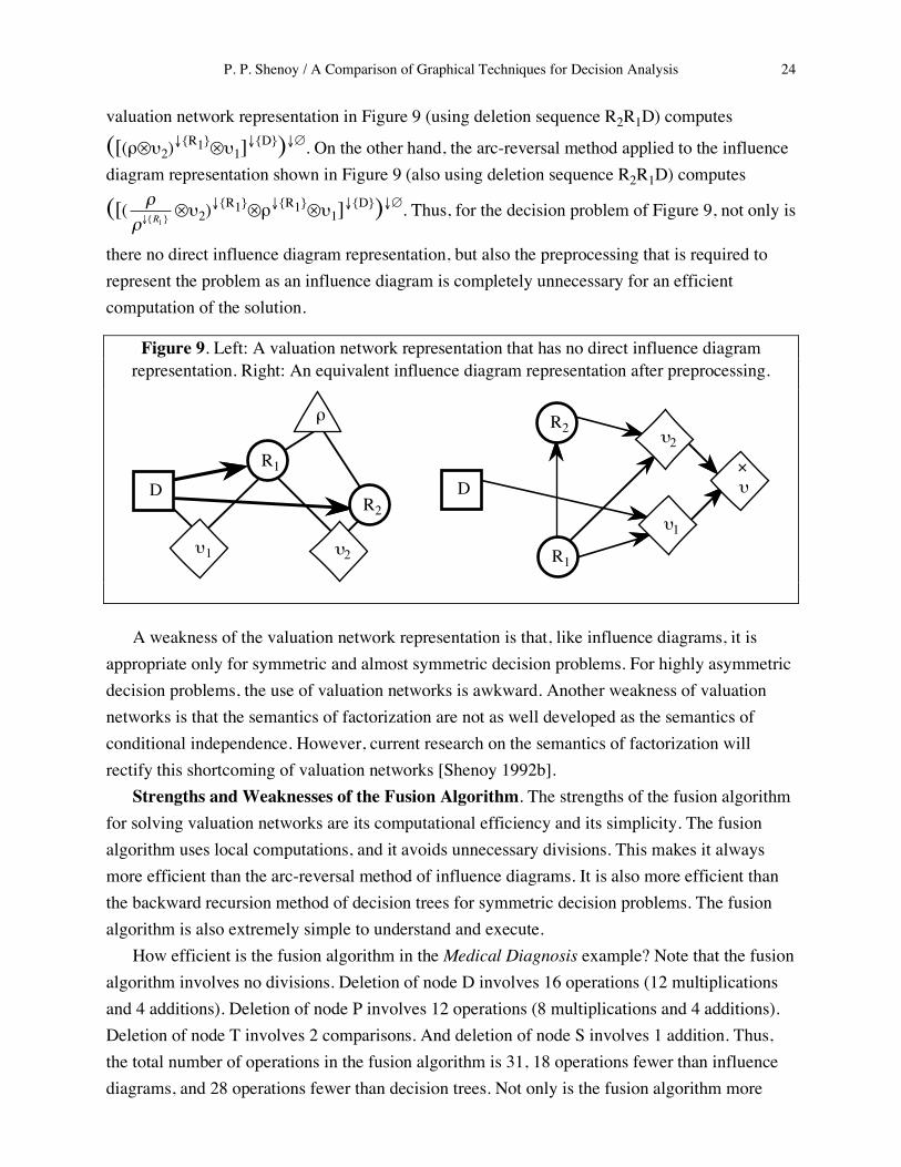
P. P. Shenoy / A Comparison of Graphical Techniques for Decision Analysis 24
valuation network representation in Figure 9 (using deletion sequence R2R1D) computes
([(ρ⊗υ2)↓{R1}⊗υ1]↓{D})↓∅. On the other hand, the arc-reversal method applied to the influence diagram representation shown in Figure 9 (also using deletion sequence R2R1D) computes
([( !
!"{R1 }⊗υ2)↓{R1}⊗ρ↓{R1}⊗υ1]↓{D})↓∅. Thus, for the decision problem of Figure 9, not only is
there no direct influence diagram representation, but also the preprocessing that is required to represent the problem as an influence diagram is completely unnecessary for an efficient computation of the solution.
Figure 9. Left: A valuation network representation that has no direct influence diagram representation. Right: An equivalent influence diagram representation after preprocessing.
D
!
R1
R2
"1 "2
D
R1
R2
"1
"2
"
#
A weakness of the valuation network representation is that, like influence diagrams, it is appropriate only for symmetric and almost symmetric decision problems. For highly asymmetric decision problems, the use of valuation networks is awkward. Another weakness of valuation networks is that the semantics of factorization are not as well developed as the semantics of conditional independence. However, current research on the semantics of factorization will rectify this shortcoming of valuation networks [Shenoy 1992b]. Strengths and Weaknesses of the Fusion Algorithm. The strengths of the fusion algorithm for solving valuation networks are its computational efficiency and its simplicity. The fusion algorithm uses local computations, and it avoids unnecessary divisions. This makes it always more efficient than the arc-reversal method of influence diagrams. It is also more efficient than the backward recursion method of decision trees for symmetric decision problems. The fusion algorithm is also extremely simple to understand and execute. How efficient is the fusion algorithm in the Medical Diagnosis example? Note that the fusion algorithm involves no divisions. Deletion of node D involves 16 operations (12 multiplications and 4 additions). Deletion of node P involves 12 operations (8 multiplications and 4 additions). Deletion of node T involves 2 comparisons. And deletion of node S involves 1 addition. Thus, the total number of operations in the fusion algorithm is 31, 18 operations fewer than influence diagrams, and 28 operations fewer than decision trees. Not only is the fusion algorithm more

P. P. Shenoy / A Comparison of Graphical Techniques for Decision Analysis 25
efficient, it is also simpler to understand and execute than the arc-reversal method of influence diagrams. A weakness of the fusion algorithm is that, in the worst case, its complexity is exponential. This is not surprising because solving a decision problem is NP-hard [Cooper 1990]. In problems with many variables, the fusion algorithm is tractable only if the sizes of the frames on which combinations are done stay small. The sizes of the frames on which combinations are done depend on the sizes of the domains of the functions and also on the information constraints. We need strong independence conditions to keep the sizes of the potentials small [Shenoy 1992b]. And we need strong assumptions on the joint utility function to decompose it into small functions [Keeney and Raiffa 1976]. Of course, this weakness is also shared by decision trees and influence diagrams.
6. Conclusion We have compared the expressiveness of the three graphical representation methods for symmetric decision problems. And we have compared the computational efficiencies of the solution techniques associated with these methods. The strengths of decision trees are their flexibility that allows easy representation for asymmetric decision problems, and their simplicity. The weaknesses of decision trees are the combinatorial explosiveness of the representation, their inflexibility in representing probability models that may necessitate unnecessary preprocessing, and their modeling of information constraints. The strengths of influence diagrams are their compactness, their intuitiveness, and their use of local computation in the solution process. The weaknesses of influence diagrams are their inflexibility in representing non-causal probability models, their inflexibility in representing asymmetric decision problems, and the inefficiency of their solution process. The strengths of valuation networks are their flexibility in representing arbitrary probability models, and the efficiency and simplicity of their solution process. The weakness of valuation networks is their inflexibility for modeling asymmetric decision problems.
Acknowledgments This work is based upon work supported in part by the National Science Foundation under Grant No. SES-9213558. Any opinions, findings, and conclusions or recommendations expressed in this paper are those of the author and do not necessarily reflect the views of the National Science Foundation. I am grateful for discussions with and comments from Ali Jenzarli, Irving LaValle, Pierre Ndilikilikesha, Anthony Neugebauer, Geoff Schemmel, Leen-Kiat Soh, and anonymous referees.

P. P. Shenoy / A Comparison of Graphical Techniques for Decision Analysis 26
References
Arnborg, S., D. G. Corneil, and A. Proskurowski (1987), “Complexity of finding embeddings in a k-tree,” SIAM Journal of Algebraic and Discrete Methods, 8, 277–284.
Bertele, U. and F. Brioschi (1972), Nonserial Dynamic Programming, Academic Press, New York, NY.
Call, H. J. and W. A. Miller (1990), “A comparison of approaches and implementations for automating decision analysis,” Reliability Engineering and System Safety, 30, 115–162.
Cooper, G. F. (1990), “The computational complexity of probabilistic inference using Bayesian belief networks,” Artificial Intelligence, 42, 393–405.
Darroch, J. N., S. L. Lauritzen, and T. P. Speed (1980), “Markov fields and log-linear interaction models for contingency tables,” The Annals of Statistics, 8, 522–539.
Edwards, D. and S. Kreiner (1983), “The analysis of contingency tables by graphical models,” Biometrika, 70, 553–565.
Ezawa, K. J. (1986), “Efficient evaluation of influence diagrams,” Ph.D. dissertation, Department of Engineering-Economic Systems, Stanford University.
Fung, R. M. and R. D. Shachter (1990), “Contingent influence diagrams,” Unpublished manuscript, Advanced Decision Systems, Mountain View, CA.
Howard, R. A. (1988), “Decision analysis: Practice and promise,” Management Science, 34(6), 679–695.
Howard, R. A. (1990), “From influence to relevance to knowledge,” in Oliver, R. M. and J. Q. Smith (eds.), Influence Diagrams, Belief Nets and Decision Analysis, 3–23, John Wiley & Sons, Chichester, UK.
Howard, R. A. and J. E. Matheson (1984), “Influence diagrams,” in Howard, R. A. and J. E. Matheson (eds.), The Principles and Applications of Decision Analysis, 2, 719–762, Strategic Decisions Group, Menlo Park, CA.
Keeney, R. L. and H. Raiffa (1976), Decisions with Multiple Objectives: Preferences and Value Tradeoffs, John Wiley & Sons, New York, NY.
Kiiveri, H., T. P. Speed, and J. B. Carlin (1984), “Recursive causal models,” Journal of the Australian Mathematics Society, Series A, 36, 30–52.
Kong, A. (1986), “Multivariate belief functions and graphical models.” Ph.D. dissertation, Department of Statistics, Harvard University, Cambridge, MA.
Lauritzen, S. L. and D. J. Spiegelhalter (1988), “Local computations with probabilities on graphical structures and their application to expert systems (with discussion),” Journal of Royal Statistical Society, Series B, 50(2), 157-224.
Ndilikilikesha, P. (1991), “Potential influence diagrams,” Working Paper No. 235, School of Business, University of Kansas.
Oliver, R. M. and J. Q. Smith, eds. (1990), Influence Diagrams, Belief Networks, and Decision Analysis, John Wiley & Sons, Chichester, UK.
Olmsted, S. M. (1983), “On representing and solving decision problems,” Ph.D. dissertation, Department of Engineering-Economic Systems, Stanford University.

P. P. Shenoy / A Comparison of Graphical Techniques for Decision Analysis 27
Owen, D. L. (1984), “The use of influence diagrams in structuring complex decision problems,” in Howard, R. A. and J. E. Matheson (eds.), Readings on The Principles and Applications of Decision Analysis, 765–772, Strategic Decisions Group, Menlo Park, CA.
Pearl, J. (1988), Probabilistic Reasoning in Intelligent Systems: Networks of Plausible Inference, Morgan Kaufmann, San Mateo, CA.
Pearl, J., D. Geiger, and T. Verma (1990), “The logic of influence diagrams,” in Oliver, R. M. and J. Q. Smith (eds.), Influence Diagrams, Belief Nets and Decision Analysis, 67–88, John Wiley & Sons, Chichester, UK.
Raiffa, H. (1968), Decision Analysis: Introductory Lectures on Choices Under Uncertainty, Addison-Wesley, Reading, MA.
Raiffa, H. and R. Schlaifer (1961), Applied Statistical Decision Theory, MIT Press, Cambridge, MA.
Rege, A. and A. M. Agogino (1988), “Topological framework for representing and solving probabilistic inference problems in expert systems,” IEEE Transactions on Systems, Man, and Cybernetics, 18(3), 402–414.
Shachter, R. D. (1986), “Evaluating influence diagrams,” Operations Research, 34, 871–882. Shachter, R. D. (1988), “Probabilistic influence diagrams,” Operations Research, 36, 589–604. Shachter, R. D. and D. E. Heckerman (1987), “A backwards view for assessment,” AI Magazine,
8(3), 55-61. Shafer, G. and P. P. Shenoy (1990), “Probability propagation,” Annals of Mathematics and
Artificial Intelligence, 2(1–4), 327-352. Shenoy, P. P. (1989), “A valuation-based language for expert systems,” International Journal of
Approximate Reasoning, 3(5), 383–411. Shenoy, P. P. (1991), “Valuation-based systems for discrete optimization,” in Bonissone, P. P.,
M. Henrion, L. N. Kanal and J. F. Lemmer (eds.), Uncertainty in Artificial Intelligence, 6, 385–400, North-Holland, Amsterdam.
Shenoy, P. P. (1992a), “Valuation-based systems for Bayesian decision analysis,” Operations Research, 40(3), 463–484.
Shenoy, P. P. (1992b), “Conditional independence in uncertainty theories,” in Dubois, D., M. P. Wellman, B. D’Ambrosio, and P. Smets (eds.), Uncertainty in Artificial Intelligence: Proceedings of the Eighth Conference, 284–291, Morgan Kaufmann, San Mateo, CA.
Shenoy, P. P. (1992c), “Valuation-based systems: A framework for managing uncertainty in expert systems,” in Zadeh, L. A. and J. Kacprzyk (eds.), Fuzzy Logic for the Management of Uncertainty, 83–104, John Wiley and Sons, NY.
Shenoy, P. P. (1993), “A new method for representing and solving Bayesian decision problems,” in Hand, D. J. (ed.), Artificial Intelligence Frontiers in Statistics: AI & Statistics III, 119–138, Chapman & Hall, London.
Smith, J. E., S. Holtzman, and J. E. Matheson (1989), “Structuring conditional relationships in influence diagrams,” unpublished manuscript, Fuqua School of Business, Duke University.
Smith, J. Q. (1989), “Influence diagrams for Bayesian decision analysis,” European Journal of Operational Research, 40, 363-376.

P. P. Shenoy / A Comparison of Graphical Techniques for Decision Analysis 28
Tatman, J. A. and R. D. Shachter (1990), “Dynamic programming and influence diagrams,” IEEE Transactions on Systems, Man, and Cybernetics, 20(2), 365–379.
von Neumann, J. and O. Morgenstern (1944), Theory of Games and Economic Behavior, 1st edition, John Wiley & Sons, New York, NY.
Watson, S. R. and D. M. Buede (1987), Decision Synthesis: The Principles and Practice of Decision Analysis, Cambridge University Press, Cambridge, UK.
Wermuth, N. and S. L. Lauritzen (1983), “Graphical and recursive models for contingency tables,” Biometrika, 70, 537–552.
Whittaker, J. (1990), Graphical Models in Applied Multivariate Statistics, John Wiley & Sons, Chichester, UK.
Related Documents