A comparison of five sampling techniques to estimate fuel ... · 139 examined the performance of various sampling techniques for measuring across multiple fuelbed 140 components,

Comparison of sampling techniques for wildland fuels Study Plan 1

A C O M P A R I S O N O F S A M P L I N G 1

T E C H N I Q U E S T O E S T I M A T E 2

W I L D L A N D S U R F A C E F U E L L O A D I N G 3

I N M O N T A N E F O R E S T S O F T H E 4

N O R T H E R N R O C K Y M O U N T A I N S 5

USDA Forest Service Fire Fuels Smoke Program RWU-4405 6

Study Plan RMRS-4405-2011-185 7

March 18, 2011 8

9

ROBERT E. KEANE 10 11

USDA FOREST SERVICE, ROCKY MOUNTAIN RESEARCH STATION, MISSOULA FIRE 12 SCIENCES LABORATORY, 13

5775 W US HIGHWAY 10, MISSOULA, MT 59808 14

Email: [email protected], Phone: 406-329-4846, FAX: 406-329-4877 15

16

17

18

he use of trade or firm names in this paper is for reader information and does not imply 19 endorsement by the U.S. Department of Agriculture of any product or service. 20

This paper was written and prepared by U.S. Government employees on official time; 21 therefore, it is in the public domain and not subject to copyright. 22

23

mailto:[email protected]


Abstract. Designing fuel sampling methods that accurately and efficiently assesses fuel loads at 24 relevant spatial scales requires knowledge of each sample method’s strengths and tradeoffs. Few 25 studies have evaluated sampling methods as to their effectiveness in estimating accurate fuel 26 loadings across all surface fuel components. In this study, we will compare three sampling methods 27 (planar intercept, microplot measurement, microplot photoload) for estimating eight surface fuel 28 components (litter, duff, 1, 10, 100, 1000 hr, shrub, herb) using a duel approach where synthetic 29 fuelbeds of known fuel loadings will be created for the fine woody fuels (1, 10, 100 hr) in the 30 parking lot of the Missoula Fire Sciences Laboratory, and field sampling at various locations in 31 western Montana, USA will be used to evaluate the all fuel components. For each of the eight fuels, 32 we compare the relative differences in load values among techniques; and the differences in load 33 between each method and a reference sample. We will also evaluate various sub-methods and 34 sampling intensities within each of the three sampling methods. Totals from each method are rated 35 for how much they deviate from totals for the reference in each fuel category. Results from this 36 study will be used to guide fuel inventory and monitoring sampling designs to select the most 37 appropriate techniques for each fuel component. 38

39

Additional keywords: Fuel sampling, photo series, line intersect, fuel inventory, photoload 40

41

42


INTRODUCTION 43

The design, implementation, and evaluation of successful fuel management activities 44 ultimately depend on the accurate inventory and monitoring of the fuel loadings in forest and 45 rangeland ecosystems (Laverty and Williams 2000). Picking the proper method to sample biomass 46 of the different types of fuels, however, requires extensive knowledge of the various sampling 47 techniques and expertise to properly modify each technique to fit unique fuel components and their 48 appropriate spatial scales, sampling objective, or eventual applications. Over the past 50 years, 49 several distinct types of fuel sampling techniques have been developed to sample downed woody 50 debris and to estimate woody fuel load. Determining how well each sampling technique quantifies 51 fuels under a variety of fuel conditions and spatial scales is critical to designing efficient sampling 52 projects that assess the effects fire-exclusion, predict fire behavior, evaluate wildlife habitat, and 53 restore altered landscapes. 54

It is difficult to compare surface fuel sampling techniques for many ecological, technological, 55 and logistical reasons. Most comparison approaches compare the sampled fuelbed with actual 56 known reference loadings. Quantifying the reference or actual fuel loadings is costly and 57 sometimes impossible, because it is difficult to collect, sort, dry, and weigh all surface fuels within a 58 common ecological sampling frame (250-500 m2 plot) located in the natural environment because 59 of the huge amount of biomass and the difficulty involved in determining the appropriate fuel 60 component. Twigs, for example, are often embedded in the litter and duff so it is difficult to 61 determine if the twig is a 1 hr fuel or part of the ground fuels, and the boundary between duff and 62 mineral soil is often difficult to discern. As a result, most fuel sampling comparisons rely on 63 subsampling using microplots or smaller sampling frames that are more suited for destructive 64 sampling (Sikkink and Keane 2009). The problem there is that the standard error involved in 65 subsample estimation can overwhelm the subtle differences between sampling methods. There are 66 also major differences between sampling techniques that make comparisons difficult. The 67 commonly used planar intercept sampling, for example, is difficult to validate because the two 68 dimensional (length and height) sampling plane makes it difficult to relate to the reference 69 sampling frame because fuel loads must be destructively sampled in three dimensions (microplot; 70 length, width, and height). Loading estimates from visually based fuel sampling methods, such as 71 photo series (Fischer 1981a) and photoloads (Keane and Dickenson 2006) have major sources of 72 error due to differences between samplers. And, the major size, shape, and density differences 73 between fuel components make comparisons difficult in that each component should be quantified 74 at their inherent ecological scale. Keane et al. (2012[in prep]) found that 1 hr woody fuels varied 75 across scales much smaller than 1000 hr fuels (2 m vs 60 m). Because of these reasons, and many 76 others, there are few evaluations of the accuracy and efficiency across sampling methods. 77

This study takes a new approach in creating the reference fuelbed for comparing surface 78 fuel sampling methods. Instead of destructively collecting and weighing the reference fuel loads for 79 the fine woody fuel components in the field, we created synthetic fuelbeds using actual fuels 80 collected in the field. We collected, sorted, dried, and weighed fine woody material from forests 81 surrounding Missoula Montana to create a fuels library of 5 kg amounts of 1, 10, and 100 hr woody 82 fuel. We then created synthetic fuelbeds in a 500 m2 flat area (grass field) of known fuel loadings, 83 and sampled the area using several fuel sampling methods. We added more fuel and re-sampled 84 the area again with the various sampling methods. We also scattered the fuel in three patterns – 85 uniform, clumpy, and jackpot. This was difficult to employ for logs, duff, and litter, so we used the 86 standard approach of creating a reference plot in the field and subsampling these fuel components 87 to obtain reference loadings. Results from this study will be useful in selecting the most 88


appropriate sampling method for each fuel component, and designing sampling protocols for 89 research and management fuels inventory and monitoring efforts. 90

Background 91

Historically, fuel load sampling procedures have ranged in scope from simple and rapid visual 92 assessments to highly detailed measurements of complex fuelbeds along lines or in fixed areas that 93 take considerable time and effort. The most common visual assessment technique is the photo-94 series method that was initially developed by Maxwell (1976) and implemented by (Fischer 95 1981b). In the photo series method, fuel loads are estimated by visually matching observed fuelbed 96 conditions with sets of oblique photographs that have been taken in disparate forests and 97 rangelands settings. The fuel loads for each photographed forest and rangeland are sampled and 98 quantified (e.g. Fischer(1981a) or Sandberg(2001)); and, theoretically, the load values can then be 99 applied to sites that appear visually similar. 100

In contrast to the photo series, the transect, planar intercept, and fixed-area methods require 101 significantly more time and effort to implement because downed woody debris is actually counted. 102 The line transect method was originally introduced by Warren and Olsen (1964) and made 103 applicable to measuring coarse woody debris by Van Wagner (1968). It is an adaptable technique 104 that is rooted in probability-proportional-to-size concepts; and several variations on the original 105 technique have been developed since 1968, including those that vary the line arrangements and 106 those that apply the technique using different technologies (DeVries 1974; Hansen 1985; Nemec 107 Linnell and Davis 2002). The planar- intersect method is a variation of the line-transect method 108 that was developed specifically for sampling fine- and coarse- woody debris in forests (Brown 109 1971; Brown 1974; Brown et al. 1982). It has the same theoretical basis as the line transect (Brown 110 et al. 1982), but it uses sampling planes instead of lines. The planes are somewhat adjustable to 111 plot scale because they can be any size, shape, or orientation in space and samples can be taken 112 anywhere within the limits set for the plane (Brown 1971). The planar-transect method has been 113 used extensively in many inventory and monitoring programs because it is relatively fast and 114 simple to use (Busing et al. 2000; Waddell 2001; Lutes et al. 2006). It has also been applied in 115 research because it is considered an accurate technique for measuring downed woody fuels 116 (Kalabokidis and Omi 1998; Dibble and Rees 2005). In contrast to the probability-based methods, 117 the fixed-area or quadrat methods are based on frequency concepts and have been adapted from 118 vegetation studies to sample fuels (Mueller-Dombois and Ellenberg 1974). In fixed-area sampling, 119 a round or rectangular plot is used to defined a sampling area and all fuels within the plot boundary 120 that meet a specified criteria are measured using methods that range from destructive collection to 121 volumetric measurements (i.e. length, width, diameter). Because fixed-area plots require 122 significant investments of time and money, they are more commonly used to answer specific fuel 123 research questions rather than to monitor or inventory management areas. 124

In recent years, several new methods of assessing fuel loading have been developed to sample 125 fuel beds in innovative ways. The photoload method uses calibrated, downward-looking 126 photographs of known fuel loads to compare with conditions on the forest floor and estimate fuel 127 loadings for individual fuel categories (Keane and Dickinson 2007 [in press]-b). The stereoscopic 128 vision technique builds on the photo series by using computer-image recognition to identify large 129 woody fuels from stereoscopic photos and compute loading volume (Arcos et al. 1998; Sandberg et 130 al. 2001). Transect relascope, point relascope, and prism sweep sampling use angle gauge 131 theory to expand on the line-transect method for sampling coarse woody debris (Stahl 1998; 132 Bebber and Thomas 2003; Gove et al. 2005). Perpendicular distance sampling (Williams and 133 Gove 2003) uses probablility proportions to estimate log volumes without actually collecting 134 detailed data on all log lengths and diameters. Several comparisons have been done between the 135 traditional sampling techniques and these more contemporary methods to evaluate their 136


performance, accuracy, and bias in measuring coarse-woody debris (Delisle et al. 1988; Lutes 1999; 137 Bate et al. 2004; Jordan et al. 2004; Woldendorp et al. 2004). However, no studies have yet 138 examined the performance of various sampling techniques for measuring across multiple fuelbed 139 components, such as combinations of fine- and coarse- woody debris, live and dead shrubs, and 140 herbs on the forest floor - all of which are very important to flammability, monitoring, inventory, 141 and wildlife studies. 142

In this study, we explore how five sampling methods compare in their ability to assess downed 143 woody debris loading and also how a different set of three techniques compare when sampling 144 shrub, herb, litter, and duff load. These down woody techniques include: 1) microplot 145 measurement, 2) microplot photoload, 3) planar intercept, and 4) macroplot Photoload, and 5) 146 macroplot photo series. The microplot methods will be used to assess shrub, herb, litter and duff. 147 We will also evaluate various sampling intensities and sub-methods on their precision and 148 accuracy. We evaluate each technique based on: (1) how its estimated loading compares to a 149 reference sample; (2) how much time it requires to complete sampling; and (3) how much training 150 is needed to implement it. Our goal is to provide a guide to the tradeoffs involved in using each of 151 these fuel-load sampling techniques and provide suggestions for matching the appropriate 152 sampling method to resource- and fire-management applications. 153

154

METHODS 155

For this study, we limited our comparisons across sampling techniques to only surface fuels 156 because these elements are normally evaluated in several of the fuel sampling techniques and each 157 is an important input to fire simulation models (Rothermel 1972; Albini 1976; Reinhardt et al. 158 1997). However, the woody fuels are sampled differently from the duff, litter, shrub, and herb so 159 this study had to be divided into two phases: 160

(1) Synthetic macroplot. We will create 500 m2 synthetic fuelbeds of the fine downed dead 161 woody fuels (1, 10, and 100 hr) and employ sampling methods on these artificial fuelbeds; 162 and 163

(2) Field reference fuelbed comparisons. We employed various fuel sampling techniques to 164 estimate the loading of the shrub, herb, duff, litter and log (SHDLL) fuels. 165

Synthetic fuelbeds were used to minimize the error in estimating the reference fuel loading. Logs 166 were not included in the synthetic fuelbed because they are too big to manipulate and carry on the 167 plot and they can be easily and accurately measured in the field. Duff and litter were not included 168 on the synthetic plot because of the tremendous volume of material that would have to be 169 transported to the plot and it would have been difficult to create a realistic litter and duff layer after 170 transport to the synthetic plot. Shrub and herbs were not represented in the synthetic plot because 171 it would have been difficult to create realistic shrub and herb fuelbeds after cutting in the field and 172 transport to the site. Moreover, we would have had to kill the plants. 173

In this study, we compared sampling techniques for the four downed woody debris accepted size 174 classes (Fosberg 1970): 175

Fine Woody Debris (FWD) (Sample methods compared using the synthetic fuelbed) 176

1h fuels - particles with diameters less than 0.64 cm (<0.25 in) in diameter 177

10h fuels - particles between 0.64 and 2.54 cm (0.25-1.00 in) in diameter 178


100h fuels - particles 2.54 to 7.62 cm (1-3 in) in diameter 179

Coarse Woody Debris (CWD) (Sample methods compared using field sampled macroplot fuelbed) 180

1000h fuels consisted of fuel components greater than 7.62 cm (3+ inches) in diameter. 181 This class included all logs. 182

Ground fuels (Sample methods compared using field sampled macroplot fuelbed) 183

Litter. Freshly fallen non-woody fuels with discernable origins, such as needles, leaves, 184 bud scales, pollen cones, and seeds. 185

Duff. Decomposed organic material whose origins cannot be determined. 186

Live Fuels (Sample methods compared using field sampled macroplot fuelbed) 187

• Shrubs. Live and dead shrub material below 2 m tall. 188 • Herbs. Live and dead herbaceous material, such as grasses, sedges, and forbs, that is 189

below 2 m tall 190 • Tree. Live and dead seedling and sapling tree material below 2 m tall 191

This study consists of various sampling designs, sampling intensities, and fuelbed constructions 192 that form the experimental design of the evaluation and comparison study. The following is a 193 detailed list of the various factors evaluated in this study (Table 1): 194

• Fuel Loading. We will have five different fuelbeds with different total loadings (0.01 kg m-2, 195 0.05 kg m-2, 0.10 kg m-2, 0.15 kg m-2., 0.20 kg m-2) 196 197

• Fuel Distribution. We will have three fuel distribution treatments. 198 o Uniform. We will evenly distribute the fuels across the sampling macroplot. 199 o Patchy. We will put 80 percent of the fuel on the north half of the macroplot and 20 200

percent on the south half. 201 o Jackpot. We will put 50 percent of the fuel in the NW quadrant of the macroplot and 202

the remaining 50 percent evenly distributed across the other quadrats (16 percent 203 in each quadrat). 204 205

• Sampling method. We will evaluate five different sampling methods. 206 o Planar intercept. Employ the Brown (1974) sampling technique. 207 o Microplot measurement. Measure length and diameter of all fuel particles. 208 o Microplot photoload. Visually estimate fuel loadings on microplot. 209

210 • Sampling sub-methods. We will evaluate variations of the major sampling methods. 211

These will not be employed while sampling, but will be implemented during the analysis 212 phase. 213

o Count. Use the counts to estimate loading. 214 o Diameter-Length. Use total lengths to estimate loading. 215 o Diameters. Use traditional diameter classes, 1 cm, 2 cm, and actual diameters to 216

estimate loadings. 217 218

• Sampling Intensities. Within each method/sub-method, we will explore the effect of 219 sampling intensity on accuracy and variation. Here are examples of the investigation of 220 sampling intensity: 221


o Microplot: Explore how many microplots are needed to adequately describe fuel 222 loadings. 223

o Planar intercept: Explore how many meters of transect are needed to efficiently 224 describe fuel loading. 225

Details of photoload sampling for this study are discussed in detail in Keane and Dickinson (2007). 226 However, since this technique employs visual estimates for fuel loading, there will tend to be major 227 differences between observers depending on observer skill, experience, and ability. To account for 228 this source of variability, we will invite at least 10 participants to visually estimate fuel loadings of 229 the three components. Estimates will be made within the same 1m by 1m microplot at the same 230 time. Each participant will be asked to match the fuel loading conditions that he or she observed 231 within each of the 20 microplots to conditions portrayed in a set of downward looking photographs 232 of fuelbeds showing graduated picture sequences of increasing load. We will train each participant 233 on photoload methods and use the Holley and Keane (2010) field guide to calibrate participant 234 guess prior to sampling (Keane and Dickenson 2007). 235

The implementation of these various factors will be different between the synthetic fuelbed 236 comparison experiment and the field fuelbed comparison experiment. A complete list of field 237 equipment for establishing the synthetic plot or the field macroplots are provided in Appendix A. 238 All plot sheets are contained in Appendix B. 239

Synthetic Fuelbed Comparisons 240

We collected over 100 kg of fine woody debris from forests surrounding Missoula Montana. We 241 then sorted this fuel into the three size classes, dried the fuel at 80 deg C for three days, and 242 weighed the fuel. We then divided the fuel into 5 kg lots and stored the lots in plastic crates in a dry 243 place. We will then construct fuelbeds of known fuel weights in a rectangular area, and employ the 244 various sampling techniques on the area. There will be two references areas: (1) a large synthetic 245 macroplot within which we will sub-sample with systematically placed microplots, and (2) 246 synthetic microplots where we will vary the loading by fuel component at a 1 square meter level. 247

Macroplot 248

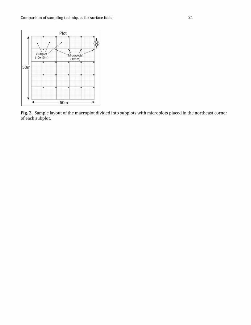
We will establish a 25 m x 20 m (500 m2) permanently-marked rectangular macroplot in an area 249 devoid of vegetation and with a minimal amount of surface complexity (parking lot, mown lawn) to 250 minimize confusion in visual estimates. The long sides (25 m) of this plot will oriented east and 251 west sides, and the short side (20 m) will run north-south. Within this plot we will stretch cloth 252 tapes at each 5 m marks (5, 10, 15, 20) and along the borders (Figure 1). We will establish a 253 microplot in the NE corner of each 5x5 m subplot. Planar intercepts will be put at 1 m intervals 254 along the 25 m sides (running north-south) and along the 20 m side (running east-west) totaling 255 24+19 or 43 transects (Figure 2). 256

We will then follow the following steps to create, measure, and evaluate sampling methods for fine 257 woody fuels: 258

(1) Choose a fuel distribution. Select one of the three fuel distribution types described 259 above. Start with the uniform fuel distribution. 260

(2) Select a fuel loading. Choose a target fuel loading starting with the lowest and 261 increasing to the highest to continually add fuel to the plot. 262

(3) Compute total fuel biomass. Multiply target fuel loading by 500 m2 to get kg of fuel to 263 put on the plot. So, the first fuel loading of 0.01 kg m-2 is 5 kg of fuel. 264

(4) Compute individual fine fuel component loadings. Compute the loadings of the 1, 10, 265 and 100 hr fuels to total the target fuel loading. Use the average proportions from the 266


FLM fuel classification (Lutes et al. 2009) or as collected in the field and represented in 267 the fuel library. So if the 1, 10, and 100 hr loadings comprise 10, 40, and 50 percent of 268 the fuelbed load, then for the first loading (0.01), the 1 hr biomass would be 0.5 kg, 10 hr 269 is 2 kg, and 100 hr is 2.5 kg. 270

(5) Spread fuel. Manually spread the fuel across the plot using the selected fuel distribution 271 method. If patchy or jackpot distribution is selected, the pre-weigh the fuel to achieve 272 the correct distributions. 273

(6) Take pictures. Photograph the fuelbed from above and from the four sides. Use a 274 scissor lift or ladder to get sufficient height to properly photographically describe the 275 fuelbed. 276

(7) Sample fuels using planar intercept. Perform the following steps to conduct the 277 planar intercept sampling. Be careful not to move or break the fuel particles Use the plot 278 form in Appendix B. The transect code is the direction of origin combined with the 279 distance on the tape so N22 signifies the transect is on the 25 m tape going north to 280 south and it is stretched between the 22 m marks. 281

a. Stretch tape. Start at the 1 m marks on the long 25 m tapes and stretch the cloth 282 tape between these two marks with the zero end at the north. 283

b. Measure fuels. Start at the north end and traverse down the stretched tape to 284 the south end and at each woody fuel particle intercept, record the particle 285 diameter and distance. 286

c. Move the tape. Once finished with the measurements, move the tape down one 287 meter and repeat steps a and b. 288

(8) Sample fuels using microplot methods. Stretch the seven cloth tapes between the 5 m 289 marks on both transects (Figure 2). 290

a. Select a microplot. Start in the NW corner of the NW 5x5m subplot. This would 291 be microplot number 1 with number 2 being the NW corner of the next subplot 292 directly to the east, and so on. Place the PVC microplot so it is in the NW corner 293 of the subplot. 294

b. Take picture. Stand on the south end of the microplot and take picture of 295 microplot and compose the picture so the microplot boundary fills the photo. 296

c. Implement photoload methods. Visually estimate the FWD loadings using the 297 photoload procedures. Record loadings on plot sheet in Appendix B. 298

d. Measure woody fuel. Measure the beginning, middle, and end diameter in mm 299 of each woody fuel particle in the microplot. Measure the diameter where it 300 intersects microplot boundaries as the beginning or end diameter. Then 301 measure the length of each fuel particle in cm. For those particles that are forked 302 or branched, measure each fork or branch as a separate particle. Use plot form in 303 Appendix B. 304

e. Go to next microplot. Pick up the PVC microplot frame and more it 5 m east to 305 the next subplot and repeat steps a through d. 306

(9) Repeat steps 1 though 8. Implement another factor in this experiment by repeating 307 steps 1-8 using new loads or new fuel distribution. 308

Microplot 309

When the entire experiment has been implemented and all fuel distributions and loadings have 310 been sampled, we will perform another finer scale experiment by creating synthetic fuelbeds at the 311 microplot scale. We will perform the exact same steps as above but there will be more fuel loadings 312 and there will be only uniform fuel distributions. We will place eight 1 m planar intercepts 313 transects at the 20 cm marks along the PVC microplot frame going north-south and east-west. The 314 only difference is that we will pick up all the fuels, separate into the three size classes and weigh 315


each fuel component to determine the difference between classes. Obviously, we will not employ 316 macroplot methods in this sub-experiment. 317

Field Fuelbed Comparisons 318

We will take a different approach for the remaining surface fuel components (SHDLL). Instead of 319 constructing pre-determined synthetic fuelbeds at the macro- and microplot scale, we will go into 320 the field and attempt to sample a wide variety of fuelbeds that contain thin to thick duff+litter 321 layers, small to large logs, and few to many shrubs and herb fuel layers. 322

We will perform these comparisons on at least five and hopefully ten study sites in western 323 Montana. We will pick these sites so that they represent different SHDLL conditions. Sites must be 324 flat, homogeneous, and representative of a major fuel type in western Montana. A 20 m by 25 m 325 rectangular plot will be located in the most homogeneous portion of the sample site. Sides will be 326 oriented in the cardinal directions. Each corner will be semi-permanently monumented using a 327 wooden stake that is labeled as to site number and corner direction (NW, NE, SE, SW). 328

Creating the perfect reference sample design that captures actual loadings by the five SHDLL 329 components for each of sample site is logistically impractical because we do not have the resources 330 to clip, collect, and weigh all the herb, shrub, and woody fuels within the 500 m2 plot and we could 331 not handle the large volume of heavy and unwieldy log material in our laboratory. Therefore, we 332 will subsample shrub, herb, and ground fuel components using nested microplots (Fig. 3). In the 333 northeast corner of each macroplot, we will establish a 1 m x 1 m microplot using a plot frame 334 made out of plastic PVC pipe (Fig. 2). Within the 25 microplots, we collected all of the fine woody 335 debris (FWD) and clipped and collected all of the living and dead shrub and herbaceous material. 336 Because this method of sampling was destructive, it was done only after data collection for all other 337 sampling methods was completed. We sorted shrub, herb, and FWD by size class into labeled paper 338 bags in the field and brought them back to the lab to be dried for 3 days in a 90oC oven and then 339 weighed to the nearest milligram. The average of the 25 microplot samples by size class 340 constituted the loading estimates for FWD, shrub, and herbaceous material in each plot. 341

Reference sampling for logs is much easier. For the 1000h fuels, we will measure the small-end 342 diameter, large-end diameter, and length of each piece of CWD greater than 7.62 cm to get a 100% 343 inventory of all logs on the macroplot at each site. We will assign a decay class (i.e. classes 1 to 5) to 344 each log using FIREMON guidelines (Lutes et al. 2006). The log volume is multiplied by a wood 345 density to obtain a weight for each log in each subplot using equations presented in Keane and 346 Dickinson (2007). The same wood density values will be used for all weight calculations; each was 347 assigned based on decay class using the density values for debris from coniferous forests suggested 348 by Brown (1974). The log weights will be summed and then divided by total plot area to calculate 349 the reference estimate of log loading. Choosing an appropriate wood density value is an important 350 decision for calculating reference loading values in this study. Many of the traditional methods for 351 measuring load assume that the density of fuel (kg m-3) is constant across all size classes and 352 species but different across various classes of decay (Brown 1974). Recently, however, research 353 has shown that there are significant differences in fuel wood density between different species, rot 354 classes, and size classes (van Wagendonk et al. 1996). We will take a sample (cookie) of each log 355 rot class represented at the site to compute our own density values. This involves cutting a “cookie” 356 or cross section of about 2-4 cm from the log somewhere at least 0.5 m from the log’s end. The 357 cookie weighed in the field and placed in a burlap bag for transport to the lab for drying and 358 weighing to compute moisture content, dry weight, and volume. 359


We will use essentially the same procedure presented for the synthetic sampling when performing 360 the field sampling with obvious exceptions. The following procedure will be employed at each 361 sample site. 362

(1) Set up macroplot. We will establish a 25 m x 20 m (500 m2) semi-permanently-marked 363 rectangular plot in a homogeneous area of the sample site. The long sides (25 m) of this 364 plot will be at the north and south sides of the plot and run east-west. Within this plot 365 we will stretch cloth tapes at each 5 m marks (5, 10, 15, 20) and along the borders 366 (Figure 1). 367

(2) Take pictures. Photograph the fuelbed from above and from the four sides. Use a 368 ladder to get sufficient height to properly photographically describe the fuelbed. 369

(3) Sample fuels using macroplot methods. We will then visually estimate fuel loadings 370 using the photo series and photoload techniques. All participants will NOT be informed 371 as to the target fuel loading and they will be trained in the protocols to effectively and 372 efficiently use these methods. 373

(4) Sample fuels using planar intercept. Perform the following steps to conduct the 374 planar intercept sampling. Be careful not to move or break the fuel particles Use the plot 375 form in Appendix B. The transect code is the direction of origin combined with the 376 distance on the tape so N22 signifies the transect is on the 25 m tape going north to 377 south and it is stretched between the 22 m marks. 378

a. Stretch tape. Start at the 1 m marks on the long 25 m tapes and stretch the cloth 379 tape between these two marks with the zero end at the north. 380

b. Measure fuels. Start at the north end and traverse down the stretched tape to 381 the south end and at each woody fuel particle intercept, record the particle 382 diameter and distance. Do this for all woody fuels including logs. 383

c. Move the tape. Once finished with the measurements, move the tape down one 384 meter and repeat steps a and b. 385

(5) Sample fuels using microplot methods. Stretch the seven cloth tapes between the 5 m 386 marks on both transects (Figure 2). 387

a. Select a microplot. Start in the NW corner of the NW 5x5m subplot. This would 388 be microplot number 1 with number 2 being the NW corner of the next subplot 389 directly to the east, and so on. Place the PVC microplot so it is in the NW corner 390 of the subplot. 391

b. Take picture. Stand on the south end of the microplot and take picture of 392 microplot and compose the picture so the microplot boundary fills the photo. 393

c. Implement photoload methods. Visually estimate the shrub, herb, and FWD 394 loadings using the photoload procedures. Record loadings on plot sheet in 395 Appendix B. 396

d. Estimate cover and height of shrub and herb. Visually estimate the cover and 397 height for all shrubs and all herbs on the plot. 398

e. Clip shrub and herbs. Cut all shrubs and herbs at the litter interface and place 399 the shrub and herb material in separate paper bags for transport back to the lab. 400 Label bags as to sample site, microplot number, date, and type (shrub, herb). 401

f. Measure woody fuel. Measure the beginning, middle, and end diameter in mm 402 of each woody fuel particle in the microplot except logs. Measure the diameter 403 where it intersects microplot boundaries as the beginning or end diameter. Then 404 measure the length of each fuel particle in cm. For those particles that are forked 405 or branched, measure each fork or branch as a separate particle. Use plot form in 406 Appendix B. 407

g. Collect woody fuel. Pick up all woody fuel and place into paper bags according 408 to 1, 10, and 100 hr size classes. Be sure to cut the sticks where they cross the 409


inside border of the PVC microplot frame. Label bags as to sample site, microplot 410 number, date, and type (1, 10, 100 hr). 411

h. Take litter and duff depths. In the NW quarter of the microplot (50x50cm 412 nanoplot) estimate the depth of litter plus duff using a plastic ruler and nail – 413 insert the nail head down through the litter duff until the head encounters the 414 mineral soil then mark the top of the litter on the nail and remove nail to 415 measure depth. Do this for nine measurements – four in the corners, four at the 416 side midpoints and in 10 cm, and one in the center. Attempt to estimate the 417 percent of that depth that is litter. 418

i. Collect the litter and duff. Pick up the litter and duff layer inside the nanoplot 419 using a shovel or trowel. Try to separate the litter and duff and store in separate 420 paper bags or burlap sacks. Label bags as to sample site, microplot number, date, 421 and type (litter, duff). 422

j. Go to next microplot. Pick up the PVC microplot frame and more it 5 m east to 423 the next subplot and repeat steps a through d. 424

(6) Measure logs. The small and large end diameters and the log length will be estimated 425 for each log in the macroplot. Log lengths are measured along the central axis of the log 426 and the length terminates once it reaches the macroplot boundary, end of log, or the 427 central axis of the log is under the litter. The rot class will be recorded for each log. Plot 428 forms are in Appendix B. 429

(7) Collect log cookies. A 2-4 cm cross sectional area will be taken from a log in each rot 430 class represented on the plot. We will select logs that represent the rot class. These 431 cookies will be placed in paper bags or sacks that will be labeled as to sample site, and 432 type (rot class). 433

Calculating loadings 434

Fine Woody Debris 435

Microplot Techniques -- For all woody fuel components, including FWD and CWD, the weight of 436 each sampled piece of debris will be calculated using the volume and wood density method. 437 Volumes are calculated as follows: 438

[ ]lsls aaaalV ()(3

++= (1) 439

where as is the cross-sectional area (m2) of the small end of the log, al is the cross-sectional area of 440 the large end (m2), and l is the length (m) (Keane and Dickinson 2007 [in press]-a). Particle weight 441 (kg m-2) will be calculated by multiplying the volume by wood density (kg m-3). Wood density will 442 be calculated by estimating the volume of the sampled cookie by immersing it in water and 443 measuring the displacement and then multiplying it by dry mass estimated by putting the cookie 444 into the oven at 80oC for three days and weighing the cookie. This procedure will be used for all 445 three reference plots: synthetic microplots, microplots within the synthetic macroplot, and 446 microplots within field macroplots 447

We will investigate several levels of sampling intensities to calculate FWD loading from the 448 microplot data. The following is a list of sub-methods used in this study followed by how the 449 loadings will be calculated for each. This includes synthetic microplots, microplots within the 450 synthetic macroplot, and microplots within field macroplots: 451

1. Count method. Calculate loading using a count. Obtain a count of all sampled woody fuel 452 particles. Then multiply this count by an average woody fuel particle weight (diameter and 453


length to get volume then multiply by density). We will also experiment with using a 454 loading by size class distribution to get loadings across all size classes. 455

2. Diameter method. Calculate loading by using the sampled middle diameter and an average 456 particle length to get volume and multiply volume to get loading. Summarize this into the 457 three FWD size classes. 458

3. Diameter-Length method. Calculate loading by computing volume of the two end-to-459 middle pieces of fuel particle and multiply by density and summarize into the three size 460 classes. 461

Planar intercept -- We will follow the procedures detailed in Brown (1971; 1974) to calculate 462 FWD downed woody fuel loadings for the planar intercept method but at two intensities. We will 463 choose diameter values for the calculations based on the dominant overstory tree at the site (see 464 Brown 1974, Table 2) except when the overstory is a mix of species (Table 1, S3 and K4). In mixed-465 species cases, we will use the composite value (Brown 1974). We will also use Brown’s (1974) 466 density values for each size class assuming non-slash fuels. Here are the two sub-methods that we 467 will investigate for the planar intercept technique: 468

1. Standard method. Calculate loading using a count by size class and Brown’s (1974) 469 sampling parameters as discussed above. 470

2. Diameter method. Calculate loading by fuel particle by using the sampled diameter to 471 calculate a loading using Brown’s (1974) parameters and our pre-sampled wood densities. 472 We will then summarize this into the three FWD size classes. 473

Photoload and Photo Series -- Loading values for both photo-based techniques will be done the 474 same by averaging across all participants. Estimates by all participants at each site were also 475 averaged to obtain loading values for each photoload macroplot. For the photo series method, 476 loadings will be assigned to each component based on each participant’s photo choice and then 477 averaged by site. 478

Reference Measurements – The reference measurements for the FWD is taken from the following 479 places depending on plot sampling frame: 480

• Synthetic macroplot – The fuel loadings by FWD fuel component are known because they 481 were used as targets to create the synthetic fuel loads. However, the FWD actual loadings 482 for each microplot is unknown so it will be approximated by the average across all 483 microplots. 484

• Synthetic microplot – The fuel loadings by FWD fuel component are known because they 485 were used as targets to create the synthetic fuel loads. 486

• Field macroplot – The FWD particles will be sorted, dried, and weighed by each microplot 487 to determine actual loadings. 488

Duff and Litter 489

We will estimate the duff and litter loadings using the depth-bulk density method using different 490 sampling intensities. We will calculate the loading of the duff and litter at each nanoplot using an 491 average depth times the bulk density. The bulk density will come from two places: (1) from the 492 destructively sampled duff and litter profile and (2) from the bulk densities in Brown (1983). The 493 reference duff and litter loadings will be calculated directly from the removed profile by separating 494 the duff and litter, drying the samples, and weighing the samples. 495

Coarse Woody Debris 496


Log loads will only be computed at the macroplot level and they will only use one sampling sub-497 method. Load reference loads will be computed by calculating log volume using equation (1), then 498 multiplying this volume by the field sampled and lab-estimated densities by rot class. Planar 499 intercept loadings will be calculated using Brown (1974) methods and the visual sampling 500 techniques (photo series and Photoload) will be averaged across all observers. 501

Shrub and Herb 502

Shrub and herb loadings are only sampled using the Photoload technique at the microplot and 503 macroplot levels. The reference loadings are estimated from the destructively removed shrub and 504 herb samples that are dried and weighed to compute loadings. 505

506

Statistical comparisons 507

Statistical comparisons in this study must account for two major issues: 1) different sampling scales 508 used for each method and 2) non-normal distribution of collected data for most fuel classes. To 509 address the differences in sampling scales in methods’ comparisons, the measured loadings from 510 the reference sample and estimated loadings from the five sampling techniques will be 511 standardized to macroplot -level for each site as described in the previous section and each fuel 512 class will be compared separately. Loading values for each site will be tested for normal 513 distribution and homogeneity of variance using Q-Q normal plots and Levene’s tests (Levene 1960). 514 Natural log transformations will be made on all fuel classes except 10h fuels to comply with 515 parametric assumptions. Log transformations of the 10h fuel loadings may only increase the lack of 516 homogeneity so we may use raw data to make these comparisons. 517

Statistical differences between the five sampling methods will be tested on the natural log of the 518 loading; or, in the case of the 10h fuels, simply on the loading values. Differences will be tested 519 using both one-way analysis of variance (ANOVA) and non-parametric Kruskal-Wallace rank sum 520 tests. For analyses where both tests produced the same interpretative results, we only present the 521 ANOVA results. Where interpretative results differed between the two analyses, we will present 522 both parametric and non-parametric results. Determining which method(s) will be responsible for 523 the significant differences will be accomplished using Tukey’s HSD and Bonferroni comparisons 524 within the ANOVA tests because they compared loading values for all methods simultaneously (i.e. 525 not pair wise) in each analysis. To test whether fuel sampling experience made a significant 526 difference to mean estimates in the photo-based methods, we ran separate one-way ANOVAs for 527 each site using each site’s reference values and the estimates of observers grouped by expertise 528 levels. 529

Sampling intensities and sub-methods will be compared to the reference conditions and across all 530 sampling methods. To simplify cross-methods comparisons, we will use some combination of the 531 worse-to-best submethod and the minimum, optimum, and maximum sampling intensities. For 532 microplots, we will use 5 and 20 for the minimum and maximum sampling intensities and compute 533 the optimum from an analysis of the variance. We will use 10 and 955 m of transect for the 534 minimum and maximum planar intercept with the optimum computed later. The following sub-535 methods and intensities: 536

• Least accurate sub-method with the minimum, optimum, and maximum sampling 537 intensities. 538

• Most accurate sub-method with min, max, and optimum sampling intensity. 539


540

SAFETY 541

The field portion of this project may be somewhat dangerous for field crews. We plan to conduct 542 daily safety sessions to remind crews of dangers in sampling surface fuels. The crews will be given 543 extensive training and the state-of-the-art safety equipment to complete their tasks. Windy days 544 when the crowns are swaying will also pose a risk to the crews, so sampling will also be curtailed 545 during these days. This is especially true during thunderstorms when wind AND lightning are 546 problems. Crews will be informed of the proper procedures to report accidents and we will train 547 some crew members in first aid in case of an accident. This project will also require endless hours 548 of driving to field sites so the proper precautions will be taken to ensure no automobile accidents 549 including defensive driving. The major safety concerns in the synthetic fuel sampling phase is 550 taking the pictures from a high vantage point, whether it be from a ladder or mechanical lift. This 551 lift has a horn to alert pedestrians and other sampling crews. Walking across the cylindrical woody 552 fuels also poses a safety hazard so proper care will be give to navigating and sampling among the 553 woody sticks to prevent slipping. 554

555

PROJECT SCHEDULE 556

We would like to complete the Synthetic fuel sampling during the 2011 calendar year and the Field 557 fuel sampling during the 2012 field season. We estimate it would take a crew of 4 approximately 558 two pay periods or one month to perform the synthetic tasks and a crew of 4 approximately 3 pay 559 periods to finish the field portion of this study. We will use the winter of 2011 and 2012 to analyze 560 the data, revise methods, and select field sample sites. We will then use the winter of 2012 and 561 2013 to analyze the data and perform the lab portion of the field collected cookies and samples. 562 The project will be written up during the summer of 2013 and delivered to a journal by October 1st, 563 2013. 564

565

PERSONNEL 566

Dr. Robert Keane has extensive experience in ecological modeling, wildland fuel science, and 567 conducting large ecological field studies. Dr. Keane will support the project through his expertise in 568 fuel sampling instrumentation and procedures, and through his experience in developing canopy 569 fuel data for FARSITE. His is primarily responsible for the field sampling design. He will also write 570 the various programs specified in this study plan. 571

572

BUDGET 573


This is an unfunded project to be supported by the FFS program of RMRS. It is estimated that this 574 project will take approximately five pay periods for a crew of four GS-5 techs (5x4x$1300) and 575 eight months of Keane’s salary ($85K) totaling approximately $111,000. 576

577

DELIVERABLES 578

This project will result in several products that will be useful to managers in any agency with 579 responsibility for fire management in conifer forests. Excepting the normal publication delays, all 580 deliverables will be available at the conclusion of the study (Fall 2013). 581

The following are expected deliverables: 582

• A journal article comparing the loadings estimated from the sampling methods with the 583 reference loadings. 584

• A USDA Forest Service GTR that describes the study and recommends a set of fuel sampling 585 procedures. 586

587

TECHNOLOGY TRANSFER 588

Technology transfer will include: 589

• The teaching of study results in various fire management courses. 590 • Presentation of study results at conferences and workshops 591 • Publication of study results in popular literature 592 593

REFERENCES 594

Albini FA (1976) 'Estimating wildfire behavior and effects.' USDA Forest Service, Intermountain 595 Forest and Range Experiment Station, General Technical Report INT-30.(Ogden, UT USA). 596

Arcos A, Alvarado E, Sandberg DV (1998) Volume estimation of large woody debris with a 597 stereoscopic vision technique. In 'Proceedings: 13th Conference on Fire and Forest 598 Meteorology'. Lorne, Australia pp. 439-447. (International Association of Wildland Fire) 599

Bate LJ, Torgersen TR, Wisdom MJ, Garton EO (2004) Performance of sampling methods to estimate 600 log characteristics for wildlife. Forest Ecology and Management 199, 83-102. 601

Bebber DP, Thomas SC (2003) Prism sweeps for coarse woody debris. Canadian Journal of Forest 602 Research 33, 1737-1743. 603

Brown JK (1971) A planar intersect method for sampling fuel volume and surface area. Forest 604 Science 17, 96-102. 605


Brown JK (1974) 'Handbook for inventorying downed woody material.' USDA Forest Service, 606 Intermountain Forest and Range Experiment Station, General Technical Report GTR-INT-607 16.(Ogden, UT, USA). 608

Brown JK, Oberheu RD, Johnston CM (1982) 'Handbook for inventorying surface fuels and biomass 609 in the Interior West.' USDA Forest Service, Intermountain Forest and Range Experiment 610 Station, General Technical Report INT-129.(Ogden, UT, USA). 611

Busing R, Rimar K, Stolte KW, Stohlgren TJ, Waddell K (2000) 'Forest health monitoring vegetation 612 pilot field methods guide: Vegetation diversity and structure, down woody debris, fuel 613 loading.' USDA Forest Service, National Forest Health Monitoring Program.(Washington, 614 D.C., USA). 615

Delisle GP, Woodard PM, Titus SJ, Johnson AF (1988) Sample size and variability of fuel weight 616 estimates in natural stands of lodgepole pine. Canadian Journal of Forest Research 18, 649-617 652. 618

DeVries PG (1974) Multi-stage line intersect sampling. Forest Science 20, 129-133. 619

Dibble AC, Rees CA (2005) Does the lack of reference ecosystems limit our science? A case study in 620 nonnative invasive plants as forest fuels. Journal of Forestry, 329-338. 621

Fischer WC (1981a) 'Photo guide for appraising downed woody fuels in Montana forests: Interior 622 ponderosa pine, ponderosa pine-larch-Douglas-fir, larch-Douglas-fir, and Interior Douglas-623 fir cover types.' USDA Forest Service Intermountain Forest and Range Experiment Station, 624 General Technical Report INT-97.(Ogden, UT USA). 625

Fischer WC (1981b) 'Photo guides for appraising downed woody fuels in Montana forests: How 626 they were made.' USDA Forest Service Intermountain Forest and Range Experiment Station, 627 Research Note INT-288.(Ogden, UT USA). 628

Fosberg MA (1970) Drying rates of heartwood below fiber saturation. Forest Science 16, 57-63. 629

Gove JH, Williams MS, Stahl G, Ducey MJ (2005) Critical point relascope sampling for unbiased 630 volume estimation of downed coarse woody debris. Forestry 78, 417-431. 631

Hansen MH (1985) Line intersect sampling of wooded strips. Forest Science 31, 282-288. 632

Harmon ME, Sexton J (1996) 'Guidelines for measurement of woody debris in forest ecosystems.' 633 U.S. LTER Network, University of Washington, Publication No. 20.(Seattle, WA, USA). 634

Hazard JW, Pickford SG (1986) Simulation studies on line intersect sampling of forest residue, part 635 II. Forest Science 32, 447-470. 636

Herbeck LA (2000) 'Analysis of down wood volme and percent ground cover for the Missouri Ozark 637 forest ecosystem project.' U.S. Department of Agriculture, Forest Service, North Central 638 Research Station, General Techincal Report NC-208.(St. Paul, MN). 639

Insightful Corporation (2003) 'S-Plus 6.2 for Windows Professional Version.' (Seattle, WA USA). 640

Jordan GJ, Ducey MJ, Gove JH (2004) Comparing line-intersect, fixed-area, and point relascope 641 sampling for dead and downed coarse woody material in a managed northern hardwood 642 forest. Canadian Journal of Forest Research 34, 1766-1775. 643


Kalabokidis KD, Omi PN (1998) Reduction of Fire Hazard through Thinning/Residue Disposal in the 644 Urban Interface. International Journal of Wildland Fire 8, 29-35. 645

Keane RE, Dickinson LJ (2007 [in press]-a) 'Photo guides for appraising downed woody fuels in 646 Montana forests: How they were made.' USDA Forest Service Rocky Mountain Research 647 Station, Research paper RMRS-RP-XXXCD.(Fort Collins, CO USA). 648

Keane RE, Dickinson LJ (2007 [in press]-b) 'The Photoload sampling technique: estimating surface 649 fuel loadings using downward looking photographs.' USDA Forest Service Rocky Mountain 650 Research Station, General Technical Report RMRS-GTR-XXX.(Fort Collins, CO USA). 651

Laverty L, Williams J (2000) 'Protecting people and sustaining resources in fire-adapted ecosystems 652 -- A cohesive strategy.' USDA Forest Service, Forest Service response to GAO Report 653 GAO/RCED 99-65.(Washington DC). 654

Levene H (1960) Robust tests for equality of variance. In 'Contributions to probability and 655 statistics'. (Eds I Olkin, SG Ghurye, W Hoeffeling, WG Madow and HB Mann) pp. 278-292. 656 (Stanford University Press: Stanford, CA) 657

Lutes DC (1999) A comparison of methods for the quantification of coarse woody debris and 658 identification of its spatial scale: A study from the Tenderfoot Experimental Forest, 659 Montana. Master of Science thesis, The University of Montana. 660

Lutes DC, Keane RE, Caratti JF, Key CH, Benson NC, Sutherland S, Gangi LJ (2006) 'FIREMON: Fire 661 effects monitoring and inventory system.' USDA Forest Service Rocky Mountain Research 662 Station, General Technical Report RMRS-GTR-164-CD.(Fort Collins, CO USA). 663

Maxwell WG (1976) 'Photo series for quantifying forest residues in the coastal Douglas-fir--664 hemlock type, coastal Douglas-fir--hardwood type.' U.S. Dept. of Agriculture, Forest Service, 665 Pacific Northwest Forest and Range Experiment Station.(Portland, OR). 666

Mueller-Dombois D, Ellenberg H (1974) 'Aims and methods of vegetation ecology.' (John Wiley and 667 Sons: New York, New York., USA) 668

Nemec Linnell AF, Davis G (2002) 'Efficiency of six line intersect sampling designs for estimating 669 volume and density of coarse woody debris.' BCMOF Vancouver Forest Region, Research 670 Section, Technical Report.(Nanaimo, BC, Canada). 671

Pickford SG, Hazard JW (1978) Simulation studies in the line intersect sampling of forest residue. 672 Forest Science 24, 469-483. 673

Reinhardt E, Keane RE, Brown JK (1997) 'First Order Fire Effects Model: FOFEM 4.0 User's Guide.' 674 USDA Forest Service Intermountain Research Station, General Technical Report INT-GTR-675 344.(Ogden, UT USA). 676

Rothermel RC (1972) 'A mathematical model for predicting fire spread in wildland fuels.' USDA 677 Forest Service Intermountain Forest and Range Experiment Station, Research Paper INT-678 115.(Ogden, Utah). 679

Sandberg DV, Ottmar RD, Cushon GH (2001) Characterizing fuels in the 21st century. International 680 Journal of Wildland Fire 10, 381-387. 681

Stahl G (1998) Transect relascope sampling - A method for the quantification of coarse woody 682 debris. Forest Science 44, 58-63. 683


Thorne MS, Skinner QD, Smith MA, Rodgers JD, Laycock WA, Cerekci SA (2002) Evaluation of a 684 technique for measuring canopy volume of shrubs. Journal of Range Management 55, 235-685 241. 686

van Wagendonk JW, Benedict JM, Sydoriak WM (1996) Physical properties of woody fuel paticles of 687 Sierra Nevada Conifers. International Journal of Wildland Fire 6, 117-123. 688

Van Wagner CE (1968) The line intersect method in forest fuel sampling. Forest Science 14, 20-26. 689

Waddell KL (2001) Sampling coarse woody debris for multiple attributes in extensive resource 690 inventories. Ecological Indicators 1, 139-153. 691

Warren WG, Olsen PF (1964) A line intersect technique for assessing logging waste. Forest Science 692 10, 267-276. 693

Williams MS, Gove JH (2003) Perpendicular distance sampling: an alternative method for sampling 694 downed coarse woody debris. Canadian Journal of Forestry Research 33, 1564-1579. 695

Woldendorp G, Keenan RJ, Barry S, Spencer DR (2004) Analysis of sampling methods for coarse 696 woody debris. Forest Ecology and Management 198, 133-148. 697

698

699

Comparison of sampling techniques for surface fuels 19

Table 1: Sampling methods and designs evaluated in this study.

Sampling frame

Sampling

Technique

Design 1 Design 2 Design 3 Design 4

Line intersect Count Traditional 2 cm size classes

1 cm size classes

Diameter

Microplot Count Traditional size classes

2 cm size classes

1 cm size classes

Center diameter

Diameter-Length

Traditional size classes

2 cm size classes

1 cm size classes

Center diameter

Photoload Traditional size classes

Macroplot Photoload Traditional size classes

Photo series Traditional size classes


Figure Captions:

Fig. 1. Sample layout of the synthetic and field macroplot divided into subplots with microplots placed in the northwest corner of each subplot.

Fig. 2. Sample design for planar intersect. Planar intersect transects were 1 meters apart in the north-south and east-west directions.


Fig. 2. Sample layout of the macroplot divided into subplots with microplots placed in the northeast corner of each subplot.


Fig. 3. Sample design for fixed area, planar intersect, and photoload methods within each site. Fixed area strip plots were established along the northern subplot edge using a width of 1 meter. Planar intersect transects were 2 meters apart in the north-south and east-west directions. Photoloads were assessed in the same microplots that were used to collect reference fuel loads. Offsets within each subplot for sampling FWD in planar-intercept method are not shown.


APPENDIX A

Equipment list


Plot setup

Compass Cloth tape (11, 25 m tapes) Wooden Stake or rebar Logger’s tape (DBH tape) GPS unit Flagging Mallet or large hammer

Sampling gear Pencils, field notebook Field sheets Calipers Clear plastic ruler at least 25 cm long 5, 100 meter cloth tapes

Microplot

Microplot frame (1x1m) with graduated marks and string across quadrants Measuring probe Flagging Plot sheets Shovel (square nose and spade) Scoop, trowel, Burlap sacks, paper bags, large boxes Gloves Sharpie and labels Nails Clear plastic ruler Calipers

Photos

Digital camera Ladder, lift Range pole

Field Sheets

Tree data – FIREMON TD sheets Herbaceous canopy cover – FIREMON PD sheet adding a species listing option Fuel depths – total depth w/ estimates of litter, duff, masticated proportions Cover Microplot – FIREMON CM plot sheet Fuel Microplot –FM sheet (see this appendix)

Plot setup sheet to record tape bearings, witness trees, and photo numbers


APPENDIX B

Plot forms

See O:\RD\RMRS\Science\FFS\Projects\FuelDynamics\stix\docs\plot_sheets

For the most up-to-date plot sheets engineered for this study. The ones presented here are usually modified by the field crews for ease of use and to save paper.


Synthetic Plot Fuel Microplot Particle Form Fuel Loading: Date: Person:

Fuel Distribution:

Microplot

Number

Diameters (mm) Length

(cm)

Rot

End Mid End


Synthetic Plot Fuel Microplot Photoload Plot Form Macroplot: Date: Crew: Page 1

Measurement Microplots

Microplot Number 1 2 3 4 5

1 hour

10 hour

100 hour

Picture ID


1 hour

10 hour

100 hour

Picture ID


1 hour

10 hour

100 hour

Picture ID


1 hour

10 hour

100 hour

Picture ID


Synthetic Plot Planar Intercept Plot Form Fuel Loading: Date: Person:

Fuel Distribution:

Transect

(North)

Diameter

(mm)

Distance

(cm)

Transect

(East)

Diameter

(mm)

Distance

(cm)


Field Plot Planar Intercept Plot Form Macroplot: Date: Crew: Page 1

Transect

(North)

Diameter

(mm)

Distance

(cm)

Transect

(East)

Diameter

(mm)

Distance

(cm)


Field Plot Fuel Microplot Plot Form Macroplot: Date: Crew: Page 1

Measurement Microplots

Num: Num: Num: Num: Num:

Photoload Estimates (kg m-2)

1 hour

10 hour

100 hour

Shrub

Herb

Nanoplot duff-litter depths (cm) (duff+litter depth/%litter)

1-NW corner

2-NE corner

3-SE corner

4-SWcorner

5-Grid 1

6-Grid 2

7-Grid 3

8-Grid 4

9-Center

Shrub and Herb measurements (canopy cover % / height cm)

Shrub

Herb

Collection Sample (y/n)

Photo number


Field Plot Log Form Macroplot: Page 1

Log

Number

Log Characteristics

Small Diameter (cm)

Large Diameter (cm)

Length (m) Decay Class Notes


Field Plot Fuel Microplot Particle Form Fuel Loading: Date: Person:

Fuel Distribution:

Microplot

Number

Diameters (mm) Length

(cm)

Rot

End Mid End

A comparison of five sampling techniques to estimate fuel ... · 139 examined the performance of various sampling techniques for measuring across multiple fuelbed 140 components,

Documents