1 A Comparison of Clustering and Scheduling Techniques for Embedded Multiprocessor Systems Vida Kianzad and Shuvra S. Bhattacharyya Department of Electrical and Computer Engineering, and Institute for Advanced Computer Studies, University of Maryland, College Park MD 20742, USA {vida, ssb}@eng.umd.edu Abstract. In this paper we extensively explore and illustrate the effectiveness of the two-phase decomposition of scheduling — into clustering and cluster-scheduling or merging — and mapping task graphs onto embedded multiprocessor systems. We describe efficient and novel partitioning (cluster- ing) and scheduling techniques that aggressively streamline interprocessor communication and can be tuned to exploit the significantly longer compilation time that is available to embedded system design- ers. The increased compile-time tolerance results because embedded multiprocessor systems are typi- cally designed as final implementations for dedicated functions. While multiprocessor mapping strategies for general-purpose systems are usually designed with low to moderate complexity as a con- straint, embedded system design tools are allowed to employ more thorough and time-consuming opti- mization techniques [32]. We implement a framework for performance comparison of guided probabilistic-search algorithms against deterministic algorithms. We also present an experimental setup for determining the importance of different phases in scheduling and the effect of different approaches in achieving the final results. 1. Introduction This research addresses the two-phase method of scheduling [38] that was introduced by Sarkar [38] in which task clustering is performed as a compile-time pre-processing step and in advance of the actual task to processor mapping and scheduling process. This method, while sim- ple, is a remarkably capable strategy for mapping task graphs onto embedded multiprocessor architectures that aggressively streamlines interprocessor communication. This method has been explored subsequently by other researchers such as Yang and Gerasoulis [47]. In most of the fol- low-up work the focus has been on developing simple and fast algorithms for each step [24, 30, 37] and little work has been done on developing more thorough and efficient algorithms. To the

Welcome message from author
This document is posted to help you gain knowledge. Please leave a comment to let me know what you think about it! Share it to your friends and learn new things together.
Transcript

1
A Comparison of Clustering and Scheduling Techniques for Embedded Multiprocessor Systems
Vida Kianzad and Shuvra S. BhattacharyyaDepartment of Electrical and Computer Engineering, and
Institute for Advanced Computer Studies, University of Maryland, College Park MD 20742, USA
{vida, ssb}@eng.umd.edu
Abstract. In this paper we extensively explore and illustrate the effectiveness of the two-phase
decomposition of scheduling — into clustering and cluster-scheduling or merging — and mapping task
graphs onto embedded multiprocessor systems. We describe efficient and novel partitioning (cluster-
ing) and scheduling techniques that aggressively streamline interprocessor communication and can be
tuned to exploit the significantly longer compilation time that is available to embedded system design-
ers. The increased compile-time tolerance results because embedded multiprocessor systems are typi-
cally designed as final implementations for dedicated functions. While multiprocessor mapping
strategies for general-purpose systems are usually designed with low to moderate complexity as a con-
straint, embedded system design tools are allowed to employ more thorough and time-consuming opti-
mization techniques [32]. We implement a framework for performance comparison of guided
probabilistic-search algorithms against deterministic algorithms. We also present an experimental
setup for determining the importance of different phases in scheduling and the effect of different
approaches in achieving the final results.
1. Introduction
This research addresses the two-phase method of scheduling [38] that was introduced by
Sarkar [38] in which task clustering is performed as a compile-time pre-processing step and in
advance of the actual task to processor mapping and scheduling process. This method, while sim-
ple, is a remarkably capable strategy for mapping task graphs onto embedded multiprocessor
architectures that aggressively streamlines interprocessor communication. This method has been
explored subsequently by other researchers such as Yang and Gerasoulis [47]. In most of the fol-
low-up work the focus has been on developing simple and fast algorithms for each step [24, 30,
37] and little work has been done on developing more thorough and efficient algorithms. To the

2
authors’ best knowledge, there has been also little work on evaluating the idea of decomposition
or comparing scheduling algorithms that are composed of clustering and merging (i.e. two-step
scheduling algorithms) against each other or against one-step scheduling algorithms.
In [19], we took a new look at this two-step decomposition of scheduling in the context of
embedded systems and developed a more thorough and efficient evolutionary-based clustering
algorithm (called CFA) that was shown to outperform the other leading clustering algorithms.
While multiprocessor mapping and scheduling strategies for general-purpose systems are usually
designed with low to moderate complexity as a constraint, embedded system design tools can tol-
erate significantly longer compilation times due to the fact that embedded multiprocessor systems
are typically designed as final implementations for dedicated functions and modifications to
embedded system implementations are rare [32]. This flexibility allows embedded system design-
ers to employ more thorough and time-consuming optimization techniques and based on this
observation we developed a heuristic capable of exploiting this increased compile-time. We also
introduce a randomization approach to be applied to deterministic algorithms so they can exploit
increases in additional computational resources (compile time tolerance) to explore larger seg-
ments of the solution space. This approach will also provide a method for comparing the guided-
random search algorithms against deterministic algorithms in a fair setup. Few researchers have
included such comparisons in their studies [23][34].
Most existing merging techniques are simple and do not consider the timing and ordering
information generated in the clustering step. In this work, we have modified the ready-list sched-
uling algorithm to schedule groups of tasks or clusters instead of individual tasks. Our algorithm
utilizes the information from the clustering step and uses the tasks’ starting times as determined
during the clustering step to assign priorities to the clusters. We call the employed merging algo-
rithm the Clustered Ready List Scheduling Algorithm or CRLA.
Our contribution in this paper is as follows: We first evaluate a number of leading cluster-
ing algorithms such as CFA (an evolutionary algorithm based clustering algorithm introduced in
[19]), Sarkar’s Internalization Algorithm (SIA) [38] and Yang and Gerasoulis’s Dominant

3
Sequence Clustering (DSC) algorithm [47] in conjunction with a cluster-scheduling or merging
algorithm called CRLA and show that the choice of clustering algorithm can significantly change
the overall performance of the scheduling. We address the potential inefficiency implied in using
the two phases of clustering and merging with no interaction between the phases and introduce a
solution that while taking advantage of this decomposition increases the overall performance of
the resulting mappings. Next, we present a general framework for performance comparison of
guided random-search algorithms against deterministic algorithms and an experimental setup for
comparison of one-step against two-step scheduling algorithms. This framework helps to deter-
mine the importance of different steps in the scheduling problem and effect of different
approaches in the overall performance of the scheduling. We present the results of an extensive
experimental study that show that decomposition of the scheduling process indeed improves the
overall performance and that the quality of the solutions depends on the quality of the clusters
generated in the clustering step. We also discuss why the parallel execution time metric is not a
sufficient measure for performance comparison of clustering algorithms.
This paper is organized as follows. In the next section we present the background, notation
and definitions used in this paper. In section 3 we state the problem and our proposed framework.
In section 4, we present the input graphs we have used in our experiments. Experimental results
are given in section 5 and we conclude the paper in section 6 with a summary of the paper and
conclusions.
2. Background and Problem Statement
We represent the applications that are to be mapped into parallel implementations in terms
of the widely-used task graph model. A task graph is a directed acyclic graph (DAG) ,
where
• is the set of task nodes, which are in one-to-one correspondence with the computational tasks
in the application .
• is the set of communication edges (each member is an ordered pair of tasks).
• denotes a function that assigns an execution time to each member of .
G V E,( )=
V
V v1 v2 … v V, , ,{ }=( )
E
t V ℵ→: V

4
• denotes a function that gives the cost (latency) of each communication edge. That
is, for all ; for all , ; and is the cost of trans-
ferring data between and if they are assigned to different processors. This notation is illus-
trated in Figure 1.
2.1 Scheduling and Clustering
The concept of clustering has been broadly applied to numerous applications and research
problems such as parallel processing, load balancing and partitioning [38][29][31]. Clustering is
also often used as a front-end to multiprocessor system synthesis tools and as a compile-time pre-
processing step in mapping parallel programs onto multiprocessor architectures. In this research
we are only interested in the latter context, where given a task graph and infinite number of fully-
connected processors, the objective of clustering is to assign tasks to processors. In this context,
clustering is used as the first step to scheduling parallel architectures and is used to group basic
tasks into subsets that are to be executed on the same processor. Once the clusters of tasks are
formed, the task execution ordering of each processor will be determined and tasks will run
C V: V ℵ→×
C v v,( ) 0≡ V C v1 v2,( ) C v2 v1,( )= v1 v2 C v1 v2,( )
v1 v2
V1
V2 V3
V4 V5
V6V7
V8
V9
10
20 20
22 22
105
10
40
20 50
95100
30
50100
5010
60
Edge, eiIPC Cost
Ci
(V1,V2) 20
(V1,V3) 50
(V2,V4) 95
(V2,V5) 100
(V3,V6) 30
(V4,V7) 50
(V5,V8) 100
(V6,V9) 50
(V7,V8) 10
(V8,V9) 60
Task Node
Vi
Execution Timeti
V1 10
V2 20
V3 20
V4 22
V5 22
V6 10
V7 5
V8 10
V9 40
G V E,( ) V, 9 E, 10= =
t V1( ) 10 t V2( ), 20 … t V9( ), , 40= = =
C V1 V2,( ) 20 C V1 V3,( ), 50 … C V8 V9,( ), , 60= = =
e1 V1 V2,( ) e2, V1 V3,( ) … e10, , V8 V9,( )= = =
Figure 1: An example of a task graph with 9 task nodes and 10 communication edges

5
sequentially on each processor with zero intracluster overhead. The target architecture for the clus-
tering step is a clique (a clique is a graph such that each node pair is joined by an edge, i.e. the
graph is fully connected and every node is connected to ( ) other nodes.) of infinite number
of processors. The justification for clustering is that if two tasks are clustered together and are run-
ning on the same processor when an unbounded number of processors are available then they
should also be mapped to the same processor under a processor constraint, i.e. when the number of
processors is finite [38].
In general, regardless of the employed communication network model, in the presence of
heavy interprocessor communication, clustering tends to adjust the communication and computa-
tional time by changing the granularity of the program and forming coarser grain graphs. A per-
fect clustering algorithm is considered to have a decoupling effect on the graph, i.e. it should
cluster tasks that are heavily dependent (data dependency is relative to the amount of data they
exchange or the communication cost) together and form composite nodes that can be treated as
nodes in another task graph. After performing clustering and forming the new graph with compos-
ite task nodes, there has to be a scheduling algorithm to map the new and simpler graph to the
final target architecture. To satisfy this, clustering and list scheduling (and a variety of other
scheduling techniques) are used in a complementary fashion in general. Consequently, clustering
typically is first applied to constrain the remaining steps of synthesis, especially scheduling, so
that they can focus on strategic processor assignments.
The clustering goal (as well as the overall goal for this decomposition scheme) is to mini-
mize the parallel execution time while mapping the application to a given target architecture. The
parallel execution time (or simply parallel time) is defined by the following expression:
, (1)
where ( ) is the length of the longest path between node and the source
(sink) node in the scheduled graph, including all of the communication and computation costs in
that path, but excluding from . Here, by the scheduled graph, we mean the task
V 1–
τP max tlevel vx( ) blevel vx( )+ vx V∈( )=
tlevel vx( ) blevel vx( ) vx
t vx( ) tlevel vx( )

6
graph with all known information about clustering and task execution ordering modeled using
additional zero-cost edges. In particular, if and are clustered together, and is scheduled
to execute immediately after , then the edge is inserted in the scheduled graph.
Although a number of innovative clustering and scheduling algorithms exist to date, none
of these provide a definitive solution to the clustering problem. Some prominent examples of
existing clustering algorithms are:
• Dominant sequence clustering (DSC) by Yang and Gerasoulis [47],
• Linear clustering by Kim and Browne [20], and
• Sarkar's internalization algorithm (SIA) [38].
In the context of embedded system implementation, one limitation shared by many exist-
ing clustering and scheduling algorithms is that they have been designed for general purpose com-
putation. In the general-purpose domain, there are many categories of applications for which short
compile time is of major concern. In such scenarios, it is highly desirable to ensure that an appli-
cation can be mapped to an architecture within a matter of seconds. Thus, the clustering tech-
niques of Sarkar, Kim, and especially, Yang have been designed with low computational
complexity as a major goal.
However, in embedded application domains, such as signal/image/video processing, the
quality of the synthesized solution is by far the most dominant consideration, and designers of
such systems can often tolerate compile times on the order of hours or even days — if the synthe-
sis results are markedly better than those offered by low complexity techniques. We have
explored a number of approaches for exploiting this increased compile-time-tolerance. These will
be presented in sections 3.1 and 3.2. The first approach is based on genetic algorithms and is
briefly introduced in 2.2 and explored further in section 3.1.
In this paper, we assume a clique topology for the interconnection network where any
number of processors can perform interprocessor communication simultaneously. We also assume
dedicated communication hardware that allows communication and computation to be performed
v1 v2 v2
v1 v1 v2,( )

7
concurrently and we also allow communication overlap for tasks residing in one cluster.
2.2 Genetic Algorithms
Given the intractable nature of clustering and scheduling problems and the promising per-
formance of Genetic Algorithms (GA) on similar problems, it’s natural to consider a solution
based on GAs, which may offer some advantages over traditional search techniques. GAs,
inspired by observation of the natural process of evolution, are frequently touted to perform well
on nonlinear and combinatorial problems [15]. They operate on a population of solutions rather
than a single solution in the search space, and due to the domain independent nature of GA’s, they
guide the search solely based on the fitness evaluation of candidate solutions to the problem,
whereas heuristics often rely on very problem-specific knowledge and insights to get good results.
A genetic algorithm starts with an initial population of solutions. In a typical genetic algo-
rithm, the search space of all possible solutions of the problem is being mapped onto a set of finite
strings (chromosomes) over a finite alphabet and hence each of the individual solutions is repre-
sented by an array or strings of values. This population is initially generated randomly and
evolves through generations. The ability of each individual solution to be carried over to different
generations is directly related to it fitness. The fitness of each individual basically determines how
well the solution performs in regard to the objectives of the problem. Genetic operators are also
employed to generate new solutions. The basic operators of such a genetic algorithm that are
applied to candidate solutions to form new and improved solutions are crossover, mutation and
reproduction [15]. The crossover operator is defined as a mechanism for incorporating the
attributes of two parents into a new individual. The mutation operator is a mechanism for intro-
ducing necessary attributes into an individual when those attributes do not already exist within the
current population of solutions. Reproduction is analogous to Darwinian survival of the fittest
creature and is the process in which individual strings are selected according to their fitness value
to be passed to the next generation [13][15]. More details about our solution representation and
operator (crossover, mutation, etc.) implementation are given in section 3.
A survey of the literature reveals a large number of papers devoted to the scheduling prob-

8
lem while there are no GA approaches to task graph clustering. As discussed earlier in 2.1, the 2-
phase decomposition of scheduling problem offers unique advantages that are worth further
investigation and experimented thoroughly. Consequently, in this paper we develop efficient GA
approaches to clustering and mapping/merging task graphs.
2.3 Existing Approaches
IPC-conscious scheduling algorithms have received high attention in the literature and a
great number of them are based on the framework of clustering algorithms. This group of algo-
rithms, which are the main interest of this paper, have been considered as scheduling heuristics
that directly emphasize reducing the effect of IPC to minimize the parallel execution time
[38][47][24][26]. Among existing clustering approaches are Sarkar’s Internalization Algorithm
(SIA) [38] and the Dominant Sequence Clustering (DSC) algorithm of Yang and Gerasoulis [47].
Sarkar’s clustering algorithm has relatively low complexity. It starts with a complete solu-
tion and iteratively makes local changes to it, and thus is likely to be trapped in local minima.
DSC, on the other hand, builds the solution incrementally. It makes changes with regard to the
global impact on the parallel execution time, but only accounts for the local effects of these
changes, and this can lead to the accumulation of suboptimal decisions, especially for large task
graphs with high communication costs, and graphs with multiple critical paths. Nevertheless, this
algorithm has been shown to be capable of producing very good solutions, and it is especially
impressive given its low complexity.
In comparison to the high volume of research work on the clustering phase, there has been
little research on the cluster-scheduling or merging phase. Among a few merging algorithms are
Sarkar’s task assignment algorithm [38] and Yang’s Ready Critical Path (RCP) algorithm [45].
Sarkar’s merging algorithm is a modified version of list scheduling with tasks being prioritized
based on their ranks in a topological sort ordering. This algorithm has relatively high time com-
plexity. Yang’s merging algorithm is part of the scheduling tool PYRROS [46], and is a low com-
plexity algorithm based on the load-balancing concept. Since merging is the process of scheduling
and mapping the clustered graph onto the target embedded multiprocessor system, it is expected

9
to be as efficient as a scheduling algorithm that works on a non-clustered graph. Both of these
algorithms lack this motive by oversimplifying assumptions such as assigning an ordering-based
priority and not utilizing the (timing) information provided in the clustering step. A recent work
on physical mapping of task graphs into parallel architectures with arbitrary interconnection
topology can be found in [21]. A technique similar to Sarkar’s has been used by Lewis, et al. as
well in [27]. GLB and LLB [37] are two cluster-scheduling algorithms that are based on the load-
balancing idea. Although both algorithms utilize timing information, they are inefficient in the
presence of heavy communication costs in the task graph. GLB also makes local decisions w.r.t
cluster assignments which results in poor overall performance.
Due to the deterministic nature of SIA and DSC, neither can exploit the increased compile
time tolerance in embedded system implementation. There has been some research on scheduling
heuristics in the context of compile-time efficiency [28][24]; however, none studies the implica-
tions from the compile time tolerance point of view. Additionally, since they concentrate on
deterministic algorithms, they do not exploit compile time budgets that are larger than the
amounts of time required by their respective approaches.
There has been some probabilistic search implementation of scheduling heuristics in the
literature, mainly in the forms of simulated annealing (SA) algorithms or genetic algorithms
(GA). The simulated annealing algorithms attempt to avoid getting trapped in local minima and
have been successfully used for scheduling problems [35]. GAs have the same characteristic as
SAs regarding local minima and also have other advantages, which are discussed in section 2.2.
Hou et al. [16], Wang and Korfhage [47], Kwok and Ahmad [25], Zomaya et al. [53], and Correa
et al. [8] have proposed different genetic algorithms in the scheduling context. Hou and Correa
use similar integer string representations of solutions. Wang and Korfhage use a two-dimensional
matrix scheme to encode the solution. Kwok and Ahmad also use integer string representations,
and Zomaya et al. use a matrix of integer substrings. An aspect that all of these algorithms have in
common is a relatively complex solution representation in the underlying GA formulation. Each
of these algorithms must at each step check for the validity of the associated candidate solution

10
and any time basic genetic operators (crossover and mutation) are applied, a correction function
needs to be invoked to eliminate illegal solutions. This overhead also occurs while initializing the
first population of solutions. These algorithms also need to significantly modify the basic cross-
over and mutation procedures to be adapted to their proposed encoding scheme. We show that in
the context of the clustering/merging decomposition, these complications can be avoided in the
clustering phase, and more streamlined solution encodings can be used for clustering.
Correa et al. address compile time consumption in the context of their GA approach. In
particular, they run the lower-complexity search algorithms as many times as the number of gen-
erations of the more complex GA, and compare the resulting compile times and parallel execution
times (schedule makespans). However, this measurement provides only a rough approximation of
compile time efficiency. More accurate measurement can be developed in terms of fixed compile-
time budgets (instead of fixed numbers of generations). This will be discussed further in 3.2.
As for the complete two-phase implementation there is also a limited body of research
work providing a framework for comparing the existing approaches. Liou, et al. address this issue
in their paper [30]. They first apply three average-performing merging algorithms to their cluster-
ing algorithm and later on run the three merging algorithms without applying the clustering algo-
rithm and conclude that clustering is an essential step. They build their conclusion based on
problem- and algorithmic-specific assumptions. We also believe that reaching such a conclusion
may need a more thorough approach and a specialized framework and set of experiments. Hence,
their comparison and conclusions cannot be generalized to our context in this paper. Dikaiakos et
al. also propose a framework in [12] that compares various combinations of clustering and merg-
ing. In [37], Radulescu et al., to evaluate the performance of their merging algorithm (LLB), use
DSC as the base for clustering algorithms and compare the performance of DSC and 4 merging
algorithms (Sarkar’s, Yang’s, GLB and LLB) against the one-step MCP algorithm. They show
that their algorithm outperforms other merging algorithms used with DSC while it is not always
as efficient as MCP. In their comparison they do not take the effect of clustering algorithms into
account and only emphasize merging algorithms.

11
Some researchers [23][34] have presented comparison results for different clustering
(without merging) algorithms (classified as Unbounded Number of Clusters (UNC) scheduling
algorithms) and have left the cluster-merging step unexplored. In section 5, we show that the clus-
tering performance does not necessarily provide an accurate answer to the overall performance of
the two-step scheduling and hence cluster comparison does not provide important information
w.r.t. to the scheduling performance. Hence, a more accurate comparison approach should com-
pare the two-step against the one-step scheduling algorithms. In this research we will give a
framework for such comparisons that take the compile-time budget into account as well.
3. The Proposed Mapping Algorithm and Solution Description
3.1 CFA: Clusterization Function Algorithm
We propose a new framework for applying GAs to multiprocessor scheduling problems.
For such problems any valid and legal solution should satisfy the precedence constraints among
the tasks and every task should be present and appear only once in the schedule. Hence the repre-
sentation of a schedule for GAs must accommodate these conditions. Most of the proposed GA
methods satisfy these conditions by representing the schedule as several lists of ordered task
nodes where each list corresponds to the task nodes run on a processor. These representations are
typically sequence based [13]. Observing that conventional operators that perform well on bit-
string encoded solutions do not work on solutions represented in the forms of sequences opens up
the possibility of gaining a high quality solution by designing a well-defined representation.
Hence, our solution representation encodes scheduling-related information as a single subset of
graph edges , with no notion of an ordering among the elements of . This representation can
be used with a wide variety of scheduling and clustering problems.
Our representation of clustering exploits the view of a clustering as a subset of edges in
the task graph. Gerasoulis and Yang have suggested an analogous view of clustering in their char-
acterization of certain clustering algorithms as being edge-zeroing algorithms [14]. One of our
contributions in this paper is to apply this subset-based view of clustering to develop a natural,
efficient genetic algorithm formulation. For the purpose of a genetic algorithm, the representation
β β

12
of graph clusterings as subsets of edges is attractive since subsets have natural and efficient map-
pings into the framework of genetic algorithms.
Derived from the schema theory (a schema denotes a similarity template that represents a
subset of ), canonical GAs (which use binary representations of each solution as fixed-
length strings over the set and efficiently handle optimization problems of the form
) provide near-optimal sampling strategies over subsequent generations [5]. Fur-
thermore, binary encodings in which the semantic interpretations of different bit positions exhibit
high symmetry (e.g., in our case, each bit corresponds to the existence or absence of an edge
within a cluster) allow us to leverage extensive prior research on genetic operators for symmetric
encodings rather than forcing us to develop specialized, less-thoroughly-tested operators to han-
dle the underlying non-symmetric, non-traditional and sequence-based representation. Conse-
quently, our binary encoding scheme is favored both by schema theory, and significant prior work
on genetic operators. Furthermore, by providing no constraints on genetic operators, our encoding
scheme preserves the natural behavior of GAs. Finally, conventional GAs assume that symbols or
bits within an individual representation can be independently modified and rearranged, however a
scheduling solution must contain exactly one instance of each task and the sequence of tasks
should not violate the precedence constraints. Thus, any deletion, duplication or moving of tasks
constitutes an error. Traditional crossover and mutation operators are generally capable of pro-
ducing infeasible or illegal solutions. Under such a scenario, the GA must either discard or repair
(to make feasible) the non-viable solution. Repair mechanisms transform infeasible individuals
into feasible ones observing the fact that they may not always be successful. Our proposed
approach never generates an illegal or invalid solution, and thus saves repair-related compilation
time that would otherwise have been wasted in locating, removing or correcting invalid solutions.
Our approach to encoding clustering solutions is based on the following definition.
Definition 1: Suppose that is a subset of task graph edges. Then denotes
the clusterization function associated with . This function is defined by:
0 1,{ }l
0 1{ , }
f 0 1,{ } ℜ→:
βi fβ iE 0 1,{ }→:
β i

13
, (2)
where is the set of communication edges and denotes an arbitrary edge of this set. When
using a clusterization function to represent a clustering solution, the edge subset is taken to be
the set of edges that are contained in one cluster. To form the clusters we use the information
given in (zero and one edges) and put every pair of task nodes that are joined with zero edges
together. The set is defined as in (3):
. (3)
An illustration is shown in Figure 2. It can be seen in Figure 2.a that all the edges of the
graph are mapped to 1, which implies that the subsets are empty or . In Figure 2.b
edges are mapped to both 0s and 1s and four clusters have been formed. The associated subsets
of zero edges are given in Figure 2.c. Figure 3 shows another clusterization function and the asso-
ciated clustered graph. It can be seen in Figure 3.a that tasks , , , and do not have
any incoming or outgoing edges that are mapped to 0 and hence do not share any cluster with
other tasks. These tasks form clusters with single tasks and also are the only tasks running on the
f e( )0 if e βi∈( )
1 otherwise.
=
E e
βi
β
β
β βii 1=
n∪=
c. , ={e1, e9} {e4, e11} {e5, e14} {e8,e16}= {e1, e4, e5, e8, e9, e11, e14, e16}β a ∅= β b ∪ ∪ ∪
Figure 2. (a) An application graph representation of an FFT and the associated clusterization function ; (b) aclustering of the FFT application graph, and (c) the resulting subset of clustered edges, along with the(empty) subset of clustered edges in the original (unclustered) graph.
fβ afβbβb
β a
a.a.
1 2 3 4
5 6 7 8
9 10 11 12
e1 e2 e3e4 e5 e6 e7
e8
e9 e10 e11
e1 2 e13e14 e15 e1 6
1 1 1 1 1 1 1 1 1 1 1 1 1 1 1 1
e1 e2 e3 e4 e5 e6 e7 e8 e9 e10 e11 e12 e13 e14 e15 e16
a.
1 2 3 4
5 6 7 8
9 10 11 12
e1 e2 e3e4 e5 e6 e7
e8
e9 e10 e11e12 e13
e1 4 e15 e16
0 1 1 0 0 1 1 0 0 1 0 1 1 0 1 0
e1 e2 e3 e4 e5 e6 e7 e8 e9 e10 e11 e12 e13 e14 e15 e16
b.
β i β ∅=
βi
t2 t3 t9 t10 t12

14
processors they are assigned to. Hence, when using the clusterization function definition to map
zero edges onto clusters, tasks that are joined with zero edges are mapped onto the same clusters
and tasks with no zero edges connected to them form single-task clusters. This is shown in Figure
3.b. Given the clustered graph and clusterization function we can define a node subset (similar
to the edge subset ) that represents the clustered graph. In this definition, every subset (for
an arbitrary ) is the set of heads and tails (the head is the node to which the edge points and the
tail is the node from which the edge leaves) of edges that belong to edge subset . Hence every
clustering of a graph or a clustered graph can be represented using either the edge subset or the
node subset representation (An example of the node subset representation of a task graph is
given in Figure 3.c). In this paper the term clustering represents a clustered graph, where every
pair of nodes in each cluster is connected by a path. A clustered graph in general can have tasks
with no connections that are clustered together. In this research, however, we do not consider such
clusters. We also use the term clustering and clustered graph interchangeably.
Because it is based on clusterization functions to represent candidate solutions, we refer to
our GA approach as the clusterization function algorithm (CFA). The CFA representation offers
some useful properties that are described below:
Property 1: Given a clustering, there exists a clusterization function that generates it.
1 2 3 4
5 6 7 8
9 10 11 12
e1 e2 e3e4 e5 e6 e7
e8
e9 e10 e1 1e1 2 e13
e14 e15 e1 6
0 0 1 1 1 1 1 0 1 1 1 1 1 0 1 1
e1 e2 e3 e4 e5 e6 e7 e8 e9 e10 e11 e12 e13 e14 e15 e16
a.1 2 3 4
5 6 7 8
9 10 11 12
e1 e2 e3e4 e5 e6 e7
e8
e9 e10 e1 1e1 2 e13
e14 e15 e1 6
0 0 1 1 1 1 1 0 1 1 1 1 1 0 1 1
e1 e2 e3 e4 e5 e6 e7 e8 e9 e10 e11 e12 e13 e14 e15 e16
b.
βb e1 e2,{ } e8{ } e14{ }∪∪ e1 e2 e8 e14, , ,{ }= =
c. ca c=b
V1 V5 V6, ,{ } V2{ } V3{ } V4 V8,{ } V7 V11,{ } V9{ } V10{ }∪∪∪∪∪∪=
βa e1 e2,{ } e8{ } e14{ }∪∪ e1 e2 e8 e14, , ,{ }= =
Figure 3. (a) A clustering of the FFT application graph and the associated clusterization function . (b) Thesame clustering of the FFT application graph, and where single-task clusters are shown, (c) Node subsetrepresentation of the clustered graph.
fβ afβb
C
β Ci
i
βi
β
C

15
Proof: Our proof is derived from the function definition in (2). Given a clustering of a graph, we
can construct the clusterization function by examining the edge list. Starting from the head of
the list, for each edge (or ordered pair of task nodes) if both head and tail of the edge belong to the
same cluster ( ) then the associated edge cost would be
zero and according to (2) (this edge also belongs to i.e. ). If the head and
tail of the edge do not belong to the same cluster
( ) then . Hence by examining the
edge list we can construct the clusterization function and this concludes the proof.
Property 2: Given a clusterization function, there is a unique clustering that is generated by it.
Proof: The given clusterization function can be represented in the form of a binary array with
the length equal to where the th element of array is associated with the th edge and the
binary values determine whether the edge belongs to a cluster or not. By constructing the clusters
from this array we can prove the uniqueness of the clustering. We examine each element of the
binary array and remove the associated edge in the graph if the binary value is 1. Once we have
examined all the edges and removed the proper edges the graph is partitioned to connected com-
ponents where each connected component is a cluster of tasks. Each edge is either removed or
exists in the final partitioned graph depending on its associated binary value. Hence anytime we
build the clustering or clustered graph using the same clusterization function we will get the same
connected components, partitions or clusters, and consequently, the clustering formed by a clus-
terization function is unique.
There is also an implicit use of knowledge in CFA-based clustering. In most GA-based
scheduling algorithms, the initial population is generated by randomly assigning tasks to different
processors. The population evolves through the generations by means of genetic operators and the
selection mechanism while the only knowledge about the problem that is taken into account in the
algorithm is of a structural nature, through the verification of solution feasibility. In such GAs the
search is accomplished entirely at random considering only a subset of the search space. How-
fβ
ek ek∀ vi vj,( )= vi cx∈( ) vj cx∈( )∧( )
f ek( ) 0= βx ek βx∈
vi cx∈( ) vj cx∉( )∧( ) vi cx∉( ) vj cx∈( )∧( )∨( ) f ek( ) 1=
fβ
E i i ei

16
ever, in CFA the assignment of tasks to clusters or processors is based on the edge zeroing con-
cept. In this context, clustering tasks nodes together is not entirely random. Two task nodes will
only be mapped onto one cluster if there is an edge connecting them and they can not be clustered
together if there is no edge connecting them, because this clustering can not improve the parallel
time. Although GAs do not need any knowledge to guide their search, GAs that do have the
advantage of being augmented by some knowledge about the problem they are solving have been
shown to produce higher quality solutions and to be capable of searching the design space more
thoroughly and efficiently [1][8].
The implementation details of CFA are given in the next 3 sections.
3.1.1 Coding of Solutions
The solution to the clustering problem is a clustered graph and each individual in the ini-
tial population has to represent a clustering of the graph. As mentioned in the previous section, we
defined the clusterization function to efficiently code the solutions. Hence, the coding of an indi-
vidual is composed of an -size binary array, where and is the total number of edges
in the graph. There is a one to one relation between the graph edges and the bits, where each bit
represents the presence or absence of the edge in a cluster.
3.1.2 Initial Population
The initial population consists of binary arrays that represent different clusterings. Each
binary array is generated randomly and every bit has an equal chance for being 1 or 0.
3.1.3 Genetic Operators
As mentioned earlier, our binary encodings allow us to leverage extensive prior research
on genetic operators rather than forcing us to develop specialized, less-thoroughly-tested opera-
tors to handle the non-traditional and sequence-based representation. Hence, the genetic operators
for reproduction (mutation and crossover) that we use are the traditional two-point crossover and
the typical mutator for a binary string chromosome where we flip the bits in the string with a
n n E= E

17
given probability [15]. Both approach are very simple, fast and efficient and none of them lead to
an illegal solution, which makes the GA a repair-free GA as well.
For the selection operator we use binary tournament with replacement [15]. Here, two
individuals are selected randomly, and the best of the two individuals (according to their fitness
value) is the winner and is used for reproduction. Both winner and loser are returned to the pool
for the next selection operation of that generation.
3.1.4 Fitness Evaluation
As mentioned in section 2.2, a GA is guided in its search solely by its fitness feedback,
hence it is important to define the fitness function very carefully. Every individual chromosome
represents a clustering of the task graph. The goal of such a mapping is to minimize the parallel
time; hence, in CFA, fitness is calculated from the parallel time , (from (1)), as follows:
, (4)
where is the fitness of an individual in the current generation or population
; is the maximum or worst case parallel time computed in ;
and is the parallel time of that individual in . Thus, to evaluate the fit-
ness of each individual in the population, we must first derive the unique clustering that is given
by the associated clusterization function, and then schedule the associated clusters. Then from the
schedule, we compute the parallel time of each individual in the current population and the fitness
for each individual will be its distance from the worst solution. The more the distance the fitter the
individual is. To schedule tasks in each cluster, we have applied a modified version of list sched-
uling that abandons the restrictions imposed by a global scheduling clock, as proposed in the DLS
algorithm [41]. Since processor assignment has been taken care of in the clustering phase, the
scheduler needs only to order tasks in each cluster and assign start times. The scheduler orders
tasks based on the precedence constraints and the priority level [38] (the task with the highest
τP
Fitness Indi Pt( , ) WorstCaseParallelTime Pt( ) ParallelTime Indi P t,( )–=
Fitness Indi Pt( , ) Ind i
P t WorstCaseParallelTime Pt( ) Pt
ParallelTime Ind i Pt( , ) Pt

18
blevel has the highest priority). Additionally, to reduce the processor idle times, an insertion
scheme has been applied where a lower priority task can be scheduled ahead of a higher priority
task if it fits within the idle time of the processor and also satisfies its precedence constraints
when moved to this position. The parallel time of the associated scheduled graph constitutes the
fitness of each individual (member of the GA population) as defined in (4).
The implemented search method in our research is based on simple (non-overlapping)
genetic algorithms. Once the initial population is generated and has been evaluated, the algorithm
creates an entirely new population of individuals by selecting solution pairs from the old popula-
tion and then mating them by means of the genetic operators to produce the new individuals for
the new population. The simple GA is a desirable scheme in search and optimization, where we
are often concerned with convergence or off-line performance [15]. We also allow elitism in
CFA. Under this policy the best individual of or the current population is unconditionally car-
ried over to or the next generation to prevent losing it due to the sampling effect or genetic
operator disruption [51][10]. During our experiments we observed that different clusterings can
lead to the same fitness value, and hence in our implementation, we copy the best solutions to
the next generations. In our tests varied from 1 to 10 percent of the population so in the worst
case 90 percent of the solutions were being updated in each generation.
The process of reproduction and evaluation continues while the termination condition is not
satisfied. In this work we ran the CFA for 3000 generations regardless of the graph size or applications.
3.2 Randomized Clustering: RDSC, RSIA
Two of the well-known clustering algorithms discussed earlier in this paper, DSC and
SIA, are deterministic heuristics, while our GA is a guided random search method where elements
in a given set of solutions are probabilistically combined and modified to improve the fitness of
populations. To be fair in comparison of these algorithms, we have implemented a randomized
version of each deterministic algorithm — each such randomized algorithm, like the GA, can
exploit increases in additional computational resources (compile time tolerance) to explore larger
P t
P t 1+
n
n

19
segments of the solution space.
Since the major challenge in clustering algorithms is to find the most strategic edges to
“zero” in order to minimize the parallel execution time of the scheduled task graph, we have
incorporated randomization into to the edge selection process when deriving randomized versions
of DSC (RDSC) and SIA (RSIA). In the randomized version of SIA, we first sort all the edges
based on the sorting criteria of the algorithm i.e. the highest IPC cost edge has the highest priority.
The first element of the sorted list — the candidate to be zeroed — then is selected with probabil-
ity , where is a parameter of the randomized algorithm (we call the randomization parame-
ter); if this element is not chosen, the second element is selected with probability ; and so on,
until some element is chosen, or no element is returned after considering all the elements in the
list. In this last case (no element is chosen), a random number is chosen from a uniform distribu-
tion over (where is the set of edges that have not yet been clustered).
In the randomized version of the DSC algorithm, at each clustering step two node priority
lists are maintained: a partial free task (a task node is partially free if it is not scheduled and at least
one of its predecessors has been scheduled but not all of its predecessors have been scheduled) list
and a free task (a task node is free if all its predecessors have been scheduled) list, both sorted in
descending order of their task priorities (the priority for each task in the free list is the sum of the
task’s and . The priority value of a partial free task is defined based on the
IPC and computational cost — more details can be found in [47]). The criterion for accepting a
zeroing is that the value of of the highest priority free list does not increase by such
zeroing. Similar to RSIA, we first sort based on the sorting criteria of the algorithm, the first ele-
ment of each sorted list then is selected with probability , and so on. Further details on this gen-
eral approach to incorporating randomization into greedy, priority-based algorithms can be found
in [52], which explores randomization techniques in the context of DSP memory management.
When , clustering is always randomly performed by sampling a uniform distribu-
tion over the current set of edges, and when , the randomized technique reduces to the cor-
responding deterministic algorithm. Each randomized algorithm version begins by first applying
p p p
p
0 1 … T 1–, ,{ , } T
tlevel blevel tlevel
tlevel vx( )
p
p 0=
p 1=

20
the underlying (original) deterministic algorithm, and then repeatedly computing additional solu-
tions with a “degree of randomness” determined by . The best solution computed within the
allotted (pre-specified) compile-time tolerance (e.g., 10 minutes, 1 hour, etc.) is returned.
Through extensive experiments, we have found the best randomization parameters for RSIA and
RDSC to be 0.10 and 0.65, respectively.
Both RDSC and RSIA are capable of generating all the possible clusterings (using our
definition of clustering given in 3.1). This results because in both algorithms the base for cluster-
ing is zeroing (IPC cost of) edges by clustering the edges and all edges are visited at least once (In
RSIA edges are visited exactly once) and hence every two task nodes have the opportunity of
being mapped onto the same cluster.
3.3 Merging
Merging is the final phase of scheduling and is the process of mapping the clustered graph
to the parallel embedded multiprocessor system where a finite number of processors is available.
This process should also maintain the minimum achievable parallel time while satisfying the
resource constraints. As mentioned earlier for the merging algorithm, we have modified the
ready-list scheduling heuristic so it can be applied to a cluster of nodes (CRLA). This algorithm is
indeed very similar to the Sarkar’s task assignment algorithm except for the priority metric:
studying the existing merging techniques, we observed that if the scheduling strategy used in the
merging phase is not as efficient as the one used in the clustering phase, the superiority of the
clustering algorithm can be negatively effected. To solve this problem we implemented a merging
algorithm (clustered ready-list scheduling algorithm or CRLA) such that it can use the timing
information produced by the clustering phase. We observed that if we form the priority list in
order of increasing of tasks (or ), tasks
preserve their relative ordering that was computed in the clustering step.
, is the latest starting time of task and or the latest com-
pletion time is the latest time at which task can complete execution. Similar to Sarkar’s task
assignment algorithm, the same ordering is also maintained when tasks are sorted within clusters.
p
LSTTOPOLOGICAL SORT– ORDERING–( , ) blevel
LST v i( ) LCT vi( ) t vi( )–= v i LCT vi( )
v i

21
In CRLA (similar to Sarkar’s algorithm) initially there are no tasks assigned to the
available processors. The algorithm starts with the clustered graph and maps it to the processor
thorough iterations. In each stage, a task at the head of the priority list is selected and along
with other tasks in the same cluster is assigned to one of the processors that gives the minimum
parallel time increase from the previous iteration. For cluster to processor assignment we always
assume all the processors are idle or available. The algorithm finishes when the number of clus-
ters has been reduced to the actual number of physical processors. An outline of this algorithm is
presented in Figure 4. In the following section we explain the implementation of the overall sys-
tem.
3.4 Two-phase mapping
In order to implement the two-step scheduling techniques that were described earlier, we used
the three addressed clustering algorithms: CFA, RDSC and RSIA in conjunction with CRLA. Our
experiments were set up in two different formats that are described in the sections 3.4.1 and 3.4.2.
3.4.1 First Approach
In the first step, the clustering algorithms, being characterized by their probabilistic search
of the solution space, had to run iteratively (not once) or for a given time budget. Through exten-
p
V
p
1 Algorithm Merging (CRLA)2 Input : A clustered graph, with execution time, intercluster communication estimates, and
multiple processors (clusters) with task ordering within each cluster.3 Output : An optimized schedule of the clustered graph onto P processors.4
5 Initialize list LIST of size P such that , for
6 Initialize where s are sorted based on their blevel or (LST, TOTALORDER)
7 For to
8 If ( )
9 select a processor , s.t. the merging of cluster( ) and LIST( ) gives the best .
10 Merge cluster( ) and LIST( ).
11 Assign all the tasks on cluster( ) to processor , update LIST( ).
12 for all tasks on LIST( ) set
13 Endif14 Endfor
LIST p( ) φ← p 1 P:=
PRIORITYLIST v1 … v V,( , )← vi
j 1← V
proc vj( ) 1 … P,{ , }∉
i v j i Pτ
vj i
vj i i
i proc vk( ) i←
Figure 4. A sketch of the employed cluster-scheduling or merging algorithm (CRLA).

22
sive experimentation with CFA using small and large size graphs we found that running CFA for
3000 iterations (generations) is the best setup for CFA. CFA finds the solution to smaller size
graphs in earlier generations (~1500) but larger size graphs need more time to perform well and
hence we set the number of iteration to be 3000 for all graph sizes. We then ran CFA for this num-
ber of iterations and monitored and recorded the running time of the algorithm as well as the
resulting clustering and performance measures. We used the recorded running time of CFA for
each input graph to determine the allotted running time for RDSC or RSIA on the same graph.
This technique allows comparison under equal amounts of running time. After we found the
results of each algorithm within the specified time budget, we used the clustering information as
an input to the merging algorithm described in section 3.3 and ran it once to find the final map-
ping to the actual target architecture. In most cases, the number of clusters in CFA’s final result is
more than the number in RSIA or RDSC. RSIA tends to find solutions with smaller numbers of
clusters than the other two algorithms. To compare the performance of these algorithms we set the
number of actual processors to be less than the minimum achieved number of clusters. Through-
out the experiments we tested our algorithms for 2, 4, 8 and 16 processor architectures depending
on the graph sizes.
3.4.2 Second Approach
Although CRLA employs the timing information provided in the clustering step, the over-
all performance is still sensitive to the employed scheduling or task ordering scheme in the clus-
tering step. To overcome this deficiency we modified the fitness function of CFA to be the
merging algorithm. Hence, instead of evaluating each cluster based on its local effect (which
would be the parallel time of the clustered graph mapped to infinite processor architecture) we
evaluate each cluster based on its effect on the final mapping. Except for this modification, the
rest of the implementation details for CFA remain unchanged. RDSC and RSIA are not modified
although the experimental setup is changed for them. Consequently, instead of running these two
algorithms for as long as the time budget allows, locating the best clustering, and applying merg-

23
ing in one step, we run the overall two-step algorithm within the time budget. That is we run
RDSC (RSIA) once, apply the merging algorithm to the resulting clustering, store the results, and
start over. At the end of each iteration we compare the new result with the stored result and update
the stored result if the new one shows a better performance.
The difference between these two approaches is shown in Figure 5. Experimental results
for this approach are given in section 5.
3.5 Comparison Method
The performance comparison of a two-step scheduling algorithm against a one-step
approach is an important comparison that needs to be carefully and efficiently done to avoid any
biases towards any specific approaches. The main aim of such a comparison is to provide solid
answers to several unanswered questions regarding multi-step scheduling algorithms such as: Is a
pre-processing step (clustering here) required for multiprocessor scheduling? What is the effect of
each step on the overall performance? Should both algorithms (for clustering and merging) be
complex algorithms or an efficient clustering algorithm only requires a simple merging algo-
rithm? Can a highly efficient merging algorithm make up for a clustering algorithm with poor per-
formance? What are the important performance measures for each step?
The merging-step of a two-step scheduling technique is a modified one-step ready list sched-
uling heuristic that instead of working on single task nodes, runs on clusters of nodes. Merging algo-
RDSC/RSIA/CFA
Time Budget
DeterministicMerging (~ 0 time)
FirstApproach +
RDSC/RSIA/CFA +Deterministic Merging
Time Budget
SecondApproach
t (compile time)
t (compile time)
Time_Budget
Solution found at t =Time_Budget
Solution found at t =Time_Budget
Time_Budget
Figure 5. The diagrammatic difference between the two different implementations of the two-step clustering andcluster-scheduling or merging techniques.

24
rithms must be designed to be as efficient as scheduling algorithms and to optimize the process of
“cluster to physical processor mapping” as opposed to “task node to physical processor mapping”.
To compare the performance of a two-step decomposition scheme against a one-step
approach, since our algorithms are probabilistic (and hence time-tolerant) search algorithms (e.g.
CFA, RDSC and RSIA), we need to compare them against a one-step scheduling algorithm with
similar characteristics, i.e. capable of exploiting the increased compile time and exploring a larger
portion of the solution space. To address this need, first we selected a one-step evolutionary based
scheduling algorithm, called combined genetic-list algorithm or CGL [8], that was shown to have
outperformed the existing one-step evolutionary based scheduling algorithms (for homogeneous
multiprocessor architectures.) Next we selected a well-known and efficient list scheduling algo-
rithm (that could also be efficiently modified to employed as cluster-scheduling algorithm). The
algorithm we selected is an important generalization of list-scheduling, which is called ready-list
scheduling [43] and has been formalized by Printz [36]. Ready-list scheduling maintains the list-
scheduling convention that a schedule is constructed by repeatedly selecting and scheduling ready
nodes, but eliminates the notion of a static priority list and a global time clock. In our implemen-
tation we used the metric to assign node priorities, which is defined in section 2. We
also used the insertion technique (to exploit unused time slots) to further improve the scheduling
performance. With the same technique described in section 3.2, we also applied randomization to
the process of constructing the priority list of nodes and implemented a randomized ready-list
scheduling (RRL) technique that can exploit increases in additional computational resources
(compile time tolerance).
We then set up an experimental framework for comparing the performance of the two-step
CFA (the best of the three clustering algorithms CFA, RDSC and RSIA [19]) and CRLA against
one-step CGL and the one-step RRL algorithm. We also compared DSC and CRLA against the
RL algorithm (step 3 in Figure 6).
In the second part of these experiments, we study the effect of each step in overall sched-
uling performance. To find out if an efficient merging can make up for an average performing
blevel vx( )

25
clustering, we applied CRLA to several clustering heuristics: first we compared the performance
of the two well-known clustering algorithms (DSC and SIA) against the randomized versions of
these algorithms (RDSC and RSIA) with CRLA as the merging algorithm. Next, we compared the
performance of CFA and CRLA against RDSC and RSIA. By keeping the merging algorithm
unchanged in these sets of experiments we are able to study the effect of a good merging algo-
rithm when employed with clustering techniques that exhibit a range of performance levels.
To find out the effect of a good clustering while combined with an average-performing
merging algorithm we modified CRLA to use different metrics such as topological ordering and
static level to prioritize the tasks and compared the performance of CFA and CRLA against CFA
and the modified-CRLA. We repeated this comparison for RDSC and RSIA. In each set of these
experiments we kept the clustering algorithm fixed so we can study the effect of a good clustering
when used with different merging algorithms. The outline of this experimental set up is presented
in Figure 6.
Figure 6. Experimental setup for comparing the effectiveness of a one-step schedulingapproach versus the two-step scheduling method.
Step1. Select a well-known efficient single-phase scheduling algorithm.(insertion-based Ready-List Scheduling (RL) with blevel metric)
Step2. Modify the scheduling algorithm to geta) An algorithm that accepts clusters of nodes as input(Clustered Ready-List Scheduling (CRLA)),b) An algorithm that can exploit the increased compile time.(Randomized Ready-List Scheduling (RRL))
Step 3.Compare the performance of a one-phase scheduling algorithm vs. a two phase scheduling algorithm
a) CFA + CRLA vs. RRLb) CFA + CRLA vs. CGLc) DSC + CRLA vs RL
Step 4.Compare the importance of clustering phase vs. merging phase
a) CFA + CRLA vs. RDSC + CRLAb) CFA + CRLA vs. RSIA + CRLAc) DSC + CRLA vs. RDSC + CRLAd) SIA + CRLA vs. RSIA + CRLAe) CFA + CRLA vs. CFA + CRLA (using different metrics)f) RDSC + CRLA vs. RDSC + CRLA (using different metrics)g) RSIA + CRLA vs. RSIA + CRLA (using different metrics)

26
4. Input Benchmark Graphs
In this study, all the heuristics have been tested with three sets of input graphs. Descrip-
tions of these sets are given in the following sections.
4.1 Reference Graphs
The Reference Graphs (RG) are task graphs that have been previously used by different
researchers and addressed in the literature. This set consists of about 30 graphs (7 to 41 task
nodes). These graphs are relatively small graphs but do not have trivial solutions and expose the
complexity of scheduling very adequately. Graphs included in the RG set are given in Table 1.
4.2 Application Graphs
This set (AG) is a large set consisting of 300 application graphs involving numerical com-
putations (Cholesky factorization, Laplace Transform, Gaussian Elimination, Mean value analy-
sis, etc., where the number of tasks varies from 10 to 1000 tasks), and digital signal processing
Table 1: Referenced Graphs (RG) Set
No. Source of Task Graphs No. Source of Task Graphs
1 Ahmad & Kwok [2] (13 nodes) 16 McCreary et al. [34] (20 nodes)
2 Al-Maasarani [3] (16 nodes) 17 McCreary et al. [34] (28 nodes)
3 Al-Mouhamed [4] (17 nodes) 18 McCreary et al. [34] (28 nodes)
4 Bhattacharyya (12 nodes) 19 McCreary et al. [34] (28 nodes)
5 Bhattacharyya (14 nodes) 20 McCreary et al. [34] (32 nodes)
6 Chung & Ranka [6] (11 nodes) 21 McCreary et al. [34] (41 nodes)
7 Colin & Chretienne [7] (9 nodes) 22 Mccreary & Gill [33] (9 nodes)
8 Gerasoulis & Yang [14] (7 nodes) 23 Shirazi et al. [39] (11 nodes)
9 Gerasoulis & Yang [14] (7 nodes) 24 Teich et al. [44] (9 nodes)
10 Karplus & Strong [18] (21 nodes) 25 Teich et al. [44] (14 nodes)
11 Kruatrachue & Lewis [22] (15 nodes) 26 Wu & Gajski [50] (16 nodes)
12 Kwok & Ahmad [24] (18 nodes) 27 Wu & Gajski [50] (18 nodes)
13 Liou & Palis [30] (10 nodes) 28 Yang & Gerasoulis [47] (7 nodes)
14 McCreary et al. [34] (15 nodes) 29 Yang & Gerasoulis [48] (7 nodes)
15 McCreary et al. [34] (15 nodes)
27
(DSP). The DSP-related task graphs include -point Fast Fourier Transforms (FFTs), where
varies between 2 and 128; a collection of uniform and non-uniform multirate filter banks with
varying structures and numbers of channels; and a compact disc to digital audio tape (cd2dat)
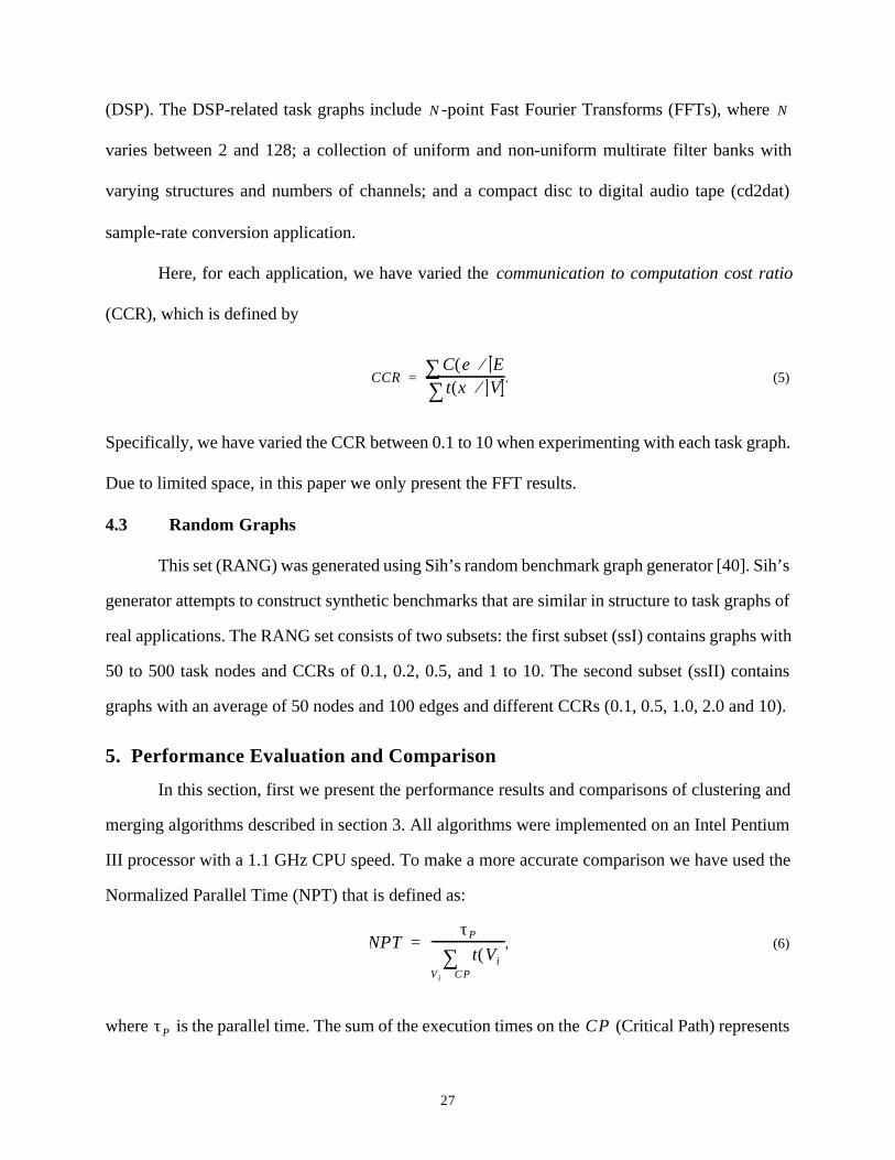
sample-rate conversion application.
Here, for each application, we have varied the communication to computation cost ratio
(CCR), which is defined by
. (5)
Specifically, we have varied the CCR between 0.1 to 10 when experimenting with each task graph.
Due to limited space, in this paper we only present the FFT results.
4.3 Random Graphs
This set (RANG) was generated using Sih’s random benchmark graph generator [40]. Sih’s
generator attempts to construct synthetic benchmarks that are similar in structure to task graphs of
real applications. The RANG set consists of two subsets: the first subset (ssI) contains graphs with
50 to 500 task nodes and CCRs of 0.1, 0.2, 0.5, and 1 to 10. The second subset (ssII) contains
graphs with an average of 50 nodes and 100 edges and different CCRs (0.1, 0.5, 1.0, 2.0 and 10).
5. Performance Evaluation and Comparison
In this section, first we present the performance results and comparisons of clustering and
merging algorithms described in section 3. All algorithms were implemented on an Intel Pentium
III processor with a 1.1 GHz CPU speed. To make a more accurate comparison we have used the
Normalized Parallel Time (NPT) that is defined as:
, (6)
where is the parallel time. The sum of the execution times on the (Critical Path) represents
N N
CCRC e( )∑ E⁄t x( )∑ V⁄
----------------------------=
NPTτP
t Vi( )V i CP∈
∑--------------------------=
τP CP

28
a lower bound on the parallel time.
Running times of the algorithms are not useful measures in our case, because we run all
the algorithms under an equal time-budget.
5.1 Results for the Referenced Graphs (RG) Set
The results of applying CFA and randomized clustering algorithms (RDSC and RSIA) to a
subset of the RG set is given in Figure 7. The x-axis shows the graph number (as given in Table
1). It was observed that in the clustering step CFA constantly performed better than or as good as
the randomized algorithms. On average CFA outperformed RDSC by 4.25%, and RSIA by 4.3%.
The results of the performance comparisons of one-step scheduling algorithms versus
two-step scheduling algorithms for a subset of the RG set are given in Figure 8. The first four
graphs show the performance of the CFA and CRLA against randomized ready list scheduling
and a one step genetic-list scheduling (CGL) algorithm [8] for 2 and 4 processor architectures. For
the RG set CFA’s results were better than RRL’s results 78% of the time, equal 15% of the time
and worse 7% of the time. CFA outperformed CGL 84.5% of the time (on the average by 17.6%)
and tied CGL 11.5% of the time. Two-step DSC tied with RL 11% of the time. DSC’s results
Figure 7. Normalized Parallel Time (NPT) generated by RDSC, RSIA and CFA for the RG set.
00.10.20.30.40.50.60.70.80.9
1
1 2 3 5 6 7 10 12 13 14 15 16 18 19 20 21 23 26 27
RG Graphs
NPT
RDSC RSIA CFA

29
were better than RL’s results 70.9% of the time and worse 18.1% of the time. It can be seen that
given two equally good one-step and two-step scheduling algorithms, the two-step algorithm can
actually gain better performance compared to the single-step algorithms. DSC is a relatively good
clustering algorithm but not as efficient as CFA or its randomized version (RDSC). However, it
can be observed that when used against a one-step scheduling algorithm, it still can offer better
solutions over 70% of the time.
To study the effect of clustering we ran our next set of experiments. The comparison
between results of merging CFA, RDSC and RSIA using CRLA onto 2 and 4-processor architec-
tures are given in Figure 9. Results of merging of DSC, RDSC, SIA and RSIA onto 2 and 4-pro-
0
0.5
1
1.5
2
2.5
1 2 3 5 6 7 10 12 13 14 15 16 18 19 20 21 23 26 27
(a) RG Graphs
NPT
RRL2
CFA2
0
0.2
0.4
0.6
0.8
1
1.2
1.4
1.6
1.8
1 2 3 5 6 7 10 12 13 14 15 16 18 19 20 21 23 26 27
(b) RG Graphs
NPT
RRL4
CFA4
00.2
0.4
0.6
0.81
1.2
1.41.6
1.8
1 2 3 5 6 7 10 12 13 14 15 16 18 19 20 21 23 26 27(d) RG Graphs
NPT
CGL4
CFA4
Figure 8. Effect of one-phase vs. two phase scheduling. RRL vs. CFA + CRLA on (a) 2 and (b) 4-processorarchitecture. CGL vs. CFA + CRLA on (c) 2 and (d) 4-processor architecture. RL vs. DSC + CRLA on (e) 2 and(f) 4-processor architecture.
0
0.5
1
1.5
2
2.5
1 2 3 5 6 7 10 12 13 14 15 16 18 19 20 21 23 26 27(c) RG Graphs
NPT
CGL2
CFA2
0
0.5
1
1.5
2
2.5
1 2 3 5 6 7 1 0 12 13 1 4 1 5 16 18 19 20 21 23 26 27
(e) RG Graphs
NPT
RL2
DSC2
0
0.2
0.4
0.6
0.8
1
1.2
1.4
1.6
1.8
1 2 3 5 6 7 10 12 13 14 15 16 18 19 20 21 23 26 27(f) RG Graphs
NPT
RL4
DSC4

30
cessor architectures using CRLA are given in Figure 10.
CFA outperformed RDSC and RSIA 52%, 84% of the time on mapping onto a 2-processor
architecture and 84% and 84% of the time on mapping onto a 4-processor architecture, respec-
tively. It can be seen that the better the quality of the clustering algorithms the better the overall
performance of the scheduling algorithms. In this case CFA clustering is better than RDSC and
RSIA and RDSC are RSIA and better than their deterministic versions.
5.2 Results for the Application Graphs (AG) Set
The result of applying the clustering and merging algorithms to a subset of application
0
0.5
1
1.5
2
2.5
1 2 3 5 6 7 10 12 13 14 15 16 18 19 20 21 23 26 27
(a) RG Graphs
NPT
RDSC2 RSIA2 CFA2
0
0.2
0.4
0.6
0.8
1
1.2
1.4
1.6
1.8
1 2 3 5 6 7 10 12 13 14 15 16 18 19 20 21 23 26 27
(b) RG Graphs
NPT
RDSC4 RSIA4 CFA4
Figure 9. Mapping of a subset of RG graphs onto (a) 2-processor, and (b) 4-processor architectures applyingCRLA to the clusters produced by the RDSC, RSIA and CFA algorithms.
0
0.5
1
1.5
2
2.5
3
1 2 3 5 6 7 10 12 13 14 15 16 18 19 20 21 23 26 27
(a) RG Graphs
NP
T
DSC2 RDSC2
00.20.40.60.8
11.21.41.61.8
1 2 3 5 6 7 10 12 13 14 15 16 18 19 20 21 23 26 27
(b) RG Graphs
NP
T
DSC4 RDSC4
0
0.5
1
1.5
2
2.5
3
1 2 3 5 6 7 10 12 13 14 15 16 18 19 20 21 23 26 27
(c) RG Graphs
NP
T
SIA2 RSIA2
00.20.40.60.8
11.21.41.61.8
1 2 3 5 6 7 10 12 13 14 15 16 18 19 20 21 23 26 27
(d) RG Graphs
NP
T
SIA4 RSIA4
Figure 10. Effect of Clustering: Performance comparison of DSC, RDSC, SIA and RSIA on RG graphs mapped to(a,c) 2-processor, (b,d) 4-processor architectures using CRLA algorithm.

31
graphs (AG) representing parallel DSP (FFT set) are given in this section. The number of nodes
for the FFT set varies between 100 to 2500 nodes depending on the matrix size .
The results of the performance comparisons of one-step scheduling algorithms versus
two-step scheduling algorithms for a subset of the FFT set are given in Figure 11, Figure 12 and
Figure 13.
The first 2 figures show the performance of the CFA and CRLA against randomized ready
list scheduling and a one step genetic-list scheduling (CGL) algorithm [8] for 2, 4 and 8 processor
architectures. For the AG set CFA’s results were better than RRL’s results 46% of the time (on
N
Figure 11. One Phase Randomized Ready-List scheduling (RRL) vs. Two Phase CFA + CRLA for a subset ofAG set graphs mapped to (a) 2-processor, (b) 4-processor, (c) 8-processor architectures.
2 4 8 16 32 640
5
10
15
(b) Matrix Dimension
AN
PT
RRL4-0.1CFA4-0.1RRL4-1CFA4-1RRL4-10CFA4-10 CCR = 0.1
CCR = 1
CCR = 10
2 4 8 16 32 640
5
10
15
20
25
30
Matrix Dimension
AN
PT
RRL2-0.1CFA2-0.1RRL2-1CFA2-1RRL2-10CFA2-10
CCR = 0.1
CCR = 0.1
CCR = 1
CCR = 1
CCR = 10
CCR = 10
2 4 8 16 32 640
1
2
3
4
5
6
7
8
(c) Matrix Dimension
AN
PT
RRL8-0.1CFA8-0.1RRL8-1CFA8-1RRL8-10CFA8-10
CCR = 0.1
CCR = 1
CCR = 10
Figure 12. One Phase CGL vs. Two Phase CFA + CRLA for RANG setI graphs mapped to (a) 2-processor, (b) 4-processor, (c) 8-processor architectures.
2 4 8 16 32 640
1
2
3
4
5
6
7
8
9
10
(c) Matrix Dimension
AN
PT
CGL8-0.1CFA8-0.1CGL8-1CFA8-1CGL8-10CFA8-10
CCR = 0.1
CCR = 1
CCR = 10
2 4 8 16 32 640
2
4
6
8
10
12
14
16
(b) Matrix Dimension
AN
PT
CGL4-0.1CFA4-0.1CGL4-1CFA4-1CGL4-10CFA4-10
CCR = 0.1
CCR = 1
CCR = 10
2 4 8 16 32 640
5
10
15
20
25
30
(a) Matrix Dimension
AN
PT
CGL2-0.1CFA2-0.1CGL2-1CFA2-1CGL2-10CFA2-10
CCR = 0.1
CCR = 1
CCR = 10

32
average by 10.45%), equal 27% of the time and worse 27% of the time. CFA outperformed CGL
64% of the time (on average by 11.1%) and tied CGL 28% of the time. Two-step DSC tied with
RL 36% of the time. DSC’s results were better than RL’s results 47% of the time (on average by
4.0%) and worse 17% of the time.
The experimental results of studying the effect of clustering on the AG set are given in
Figure 14 and Figure 15. CFA outperformed RDSC and RSIA 44% (by 11.4%) and 50% (by 3%)
of the time respectively. We observed that CFA performs its best in the presence of heavy inter-
processor communication (e.g. CCR = 10) while there is little parallelism in the graph and most
other algorithm perform very inefficiently (over 97% of the time CFA outperformed other algo-
rithms under such a scenario). This observation suggests that clustering can indeed be useful
Figure 13. One Phase Ready-list Scheduling (RL) vs. Two Phase DSC for a subset of AG set graphs mapped to(a) 2-processor, (b) 4-processor, (c) 8-processor architectures.
2 4 8 16 32 640
5
10
15
20
25
30
Matrix Dimension
AN
PT
RL2-0.1DSC2-0.1RL2-1DSC2-1RL2-10DSC2-10
CCR = 0.1
CCR = 0.1
CCR = 1
CCR = 1
CCR = 10
CCR = 10
2 4 8 16 32 640
1
2
3
4
5
6
7
8
(c) Matrix Dimension
AN
PT
RL8-0.1DSC8-0.1RL8-1DSC8-1RL8-10DSC8-10
CCR = 0.1
CCR = 1
CCR = 10
2 408 16 32 640
5
10
15
(b) Matrix Dimension
AN
PT
RL4-0.1DSC4-0.1RL4-1DSC4-1RL4-10DSC4-10
CCR = 0.1
CCR = 1
CCR = 10
2 4 8 16 32 640.2
0.4
0.6
0.8
1
1.2
1.4
1.6
1.8
(c) Matrix Dimension
AN
PT
SIA8RSIA8
SIA8
RSIA8
2 4 8 16 32 640
0.5
1
1.5
2
2.5
(a) Matrix Dimension
AN
PT
SIA2RSIA2
SIA2
RSIA2
2 4 8 16 32 640
0.5
1
1.5
2
2.5
(b) Matrix Dimension
AN
PT
SIA4RSIA4
SIA4
RSIA4
Figure 15. Effect of Clustering: Performance comparison of SIA and RSIA on a subset of AG graphs mapped to(a) 2-processor, (b) 4-processor, (c) 8-processor architecture using CRLA algorithm.

33
while used in advance of the scheduling process when the IPC cost is considerably high.
Figure 16 shows the clustering and merging results for an FFT application by CFA, and
Figure 14. Average Normalized Parallel Time from applying RDSC, RSIA and CFA to a subset of AG set (forCCR = 10), (a) results of clustering algorithms, (b) results of mapping the clustered graphs onto a 2-processorarchitecture, (c) results of mapping the clustered graphs onto a 4-processor architecture, (d) results of mappingthe clustered graphs onto an 8-processor architecture.
2 4 8 16 32 640.2
0.4
0.6
0.8
1
1.2
1.4
1.6
1.8
(d) Matrix Dimension
AN
PT
RDSC8RSIA8CFA8
RDSC8
RSIA8
CFA8
2 4 8 16 32 640
0.5
1
1.5
2
2.5
(c) Matrix Dimension
ANPT
RDSC4RSIA4CFA4
RDSC4
RSIA4
CFA4
2 4 8 16 32 64
0.4
0.5
0.6
0.7
0.8
0.9
1
1.1
(a) Matrix Dimension
ANPT
RDSC, CCR = 10
RSIA, CCR = 10
CFA, CCR = 10
2 4 8 16 32 640
0.5
1
1.5
2
2.5
(b) Matrix Dimension
AN
PT
RDSC2RSIA2CFA2
CFA2
RDSC2
RSIA2
Figure 16. Results for FFT application graphs clustered using (a) CFA (PT = 130) and (c) RDSC and RSIA (PT =150) and final mapping of FFT application graphs onto a two-processor architecture using the clustering results of(b) CFA (PT = 180) and (d) RDSC and RSIA (PT = 205).
2 4
9
1 3
75 8
11
e3
6
12
10
e1e 2
e4
e5e6
e7e8
e9e10
e 11e 12
e1 3e14
e 15e 16
(a)C1 C2
C3C4
2 4
9
1 3
7
5 8
11
6
12
10
P1 P2(b)
1 2 3 4
5 6 7 8
9 10 11 12
e1 e2 e3e4 e5 e6 e7
e8
e9 e10 e11e12 e13
e14 e15 e16
(c)
C1 C2 C3 C4
1 2
12
3 4
8
5 6
10
7
9
11
P1 P2(d)

34
the two randomized algorithms RDSC and RSIA onto the final 2-processor architecture. Our pre-
liminary studies on some of the DSP application graphs, including a wide range of filter banks,
showed that while the final configurations resulting from different clustering algorithms achieve
similar load-balancing and interprocessor communication traffic, the clustering solutions built on
CFA results are able to outperform clusterings derived by the other two algorithms.
5.3 Results for the Random Graphs (RANG) Set
In this section we have shown the experimental results (in terms of average NPT or
ANPT) for setI of the RANG task graphs. Figure 17 shows the results of comparing the one-step
randomized ready-list scheduling (RRL) against the two step CFA and CRLA. Figure 18 shows
the results of comparing the one-step probabilistic scheduling algorithm CGL [8] against the two-
step guided search scheduling algorithm CFA and CRLA. Figure 19 shows the results of compar-
ing the one-step ready-list (RL) scheduling against the two-step DSC algorithm and CRLA. The
experimental results of studying the effect of clustering are given in Figure 20 and Figure 21. For
the RANG set, CFA’s results were better than RRL’s results 82% of the time (9% improvement),
worse 10% of the time and equal 8% of the time. CFA always outperformed CGL (by 18%). Two-
Figure 17. One Phase Randomized Ready-List scheduling (RRL) vs. Two Phase CFA + CRLA for RANG setIgraphs mapped to (a) 2-processor, (b) 4-processor, (c) 8-processor architectures.
0 1 2 3 4 5 6 7 8 9 100.2
0.3
0.4
0.5
0.6
0.7
0.8
0.9
1
AN
PT
(b) setI - CCR (0.1, 0.2, 0.5, 1~10)
RRL4CFA4
RRL4 CFA4
0 1 2 3 4 5 6 7 8 9 100.2
0.4
0.6
0.8
1
1.2
1.4
1.6
1.8
(a) setI - CCR(0.1, 0.2, 0.5, 1~10)
ANPT
RRL2CFA2
RRL2 CFA2
0 1 2 3 4 5 6 7 8 9 100 . 1
0 . 2
0 . 3
0 . 4
0 . 5
0 . 6
0 . 7
0 . 8
0 . 9
1
(c) setI - CCR (0.1, 0.2, 0.5, 1~10)
AN
PT
RRL8CFA8
RRL8
CFA8

35
step DSC tied with RL 10% of the time. RL’s results were better than DSC’s 10% of the time and
worse 80% of the time (by 14%). CFA outperformed RDSC 82.3% of the time (by 5%) and tied
12.7% of the time. CFA outperformed RSIA 92.7% (by 6%) and tied otherwise.
We have not presented the results of applying different metrics graphically, however, a
summary of the results is as follows: for both test graph sets when tested with different merging
algorithms (we used CRLA with three different priority metrics: topological sort ordering, static
level and a randomly sorted priority list) each clustering algorithm did best with the original
CRLA (using metric), moderately worse with static level and worst with random level. As
shown in the literature the performance of the list scheduling algorithm highly depends on the pri-
Figure 18. One Phase CGL vs. Two Phase CFA + CRLA for RANG setI graphs mapped to (a) 2-processor, (b) 4-processor, (c) 8-processor architectures.
0 1 2 3 4 5 6 7 8 9 100.1
0.2
0.3
0.4
0.5
0.6
0.7
0.8
0.9
1
(c) setI - CCR (0.1, 0.2, 0.5, 1~10)
AN
PT
CGL8CFA8
CGL
CFA
0 1 2 3 4 5 6 7 8 9 100.2
0.3
0.4
0.5
0.6
0.7
0.8
0.9
1
1.1
1.2
(b) setI - CCR (0.1, 0.2, 0.5, 1~10)
AN
PT
CGL4CFA4
CGL
CFA
0 1 2 3 4 5 6 7 8 9 100.2
0.4
0.6
0.8
1
1.2
1.4
1.6
1.8
(a) setI - CCR (0.1, 0.2, 0.5, 1~10)
AN
PT
CGL2CFA2
CGL
CFA
Figure 19. One Phase Ready-list Scheduling (RL) vs. Two Phase DSC for RANG setI graphs mapped to (a) 2-pro-cessor, (b) 4-processor, (c) 8-processor architectures.
0 1 2 3 4 5 6 7 8 9 100.2
0.4
0.6
0.8
1
1.2
1.4
1.6
1.8
(a) setI - CCR (0.1, 0.2, 0.5, 1~10)
AN
PT
RL2DSC2
RL
DSC
0 1 2 3 4 5 6 7 8 9 100.2
0.3
0.4
0.5
0.6
0.7
0.8
0.9
1
(c) setI - CCR (0.1, 0.2, 0.5, 1~10)
AN
PT
RL8DSC8
RL
DSC
0 1 2 3 4 5 6 7 8 9 100.2
0.3
0.4
0.5
0.6
0.7
0.8
0.9
1
(b) setI - CCr (0.1, 0.2, 0.5, 1~10)
AN
PT
RL4DSC4
RL
DSC
blevel

36
ority metrics used and we observed that this was also the case for the original CRLA. Employing
the information provided in clustering in original CRLA was also another strength for the algo-
rithm. We also implemented an evolutionary based merging algorithm, however, we did not get
significant improvement in the results. We conclude that as long as the merging algorithm utilizes
the clustering information and does not restrict the processor selection to the idle processors at the
time of assignment (local decision or greedy choice), it can efficiently schedule the clusters with-
out further need for complex assignment schemes or evolutionary algorithms.
We also observed that in several cases where the results of clustering (parallel time) were
equal, CFA could outperform RDSC and RSIA after merging (this trend was not observed for
RDSC vs. DSC and RSIA vs. SIA). We also noted that there are occasional cases that two cluster-
ing results with different parallel times provide similar answers in the final mapping. There are
also cases where a worse clustering algorithm (worse parallel time) finds better final results.
Figure 20. Average Normalized Parallel Time from applying RDSC, RSIA and CFA to RANG setI, (a) results ofclustering algorithms, (b) results of mapping the clustered graphs onto a 2-processor architecture, (c) results ofmapping the clustered graphs onto a 4-processor architecture, (d) results of mapping the clustered graphs ontoan 8-processor architecture.
0 1 2 3 4 5 6 7 8 9 100.1
0.2
0.3
0.4
0.5
0.6
0.7
0.8
0.9
1
(d) setI - CCR (0.1, 0.2, 0.5, 1~10)ANPT
RDSC8RSIA8CFA8
RSIA
RDSC CFA
0 1 2 3 4 5 6 7 8 9 100.2
0.3
0.4
0.5
0.6
0.7
0.8
0.9
1
(c) setI - CCR (0.1, 0.2, 0.5, 1~10)
ANPT
RDSC4RSIA4CFA4
RSIA
RDSC
CFA
0 1 2 3 4 5 6 7 8 9 100.1
0.2
0.3
0.4
0.5
0.6
0.7
0.8
0.9
1
(a) setI-CCR(0.1, 0.2, 0.5, 1~10)
ANPT
RDSCRSIACFA
RSIA
RDSC CFA
0 1 2 3 4 5 6 7 8 9 100.2
0.4
0.6
0.8
1
1.2
1.4
1.6
(b) setI - CCR (0.1, 0.2, 0.5, 1~10)
ANPT
RDSC2RSIA2CFA2
RSIA
RDSC CFA

37
To find the reason for the first behavior, we studied the clustering results of each algorithm sep-
arately. CFA tends to use the most number of clusters when clustering tasks: there are several cases
where two clusters could be merged with no effect on the parallel time. CFA keeps them as separate
clusters. However, both RSIA and RDSC accept such clustering, i.e., when the result of clustering
doesn’t change the parallel time, and they tend to cluster as much as possible in the clustering step.
Providing more clusters and clustering only those tasks with high data dependency gives more flex-
ibility to the merging algorithm for mapping the results of CFA. This characteristic of CFA is the
main reason that even in case of similar parallel time for clustering results, CFA is still capable of
getting better overall performance.
For the second behavior we believe that the reason is behind the scheduling scheme (or task
0 1 2 3 4 5 6 7 8 9 100.2
0.4
0.6
0.8
1
1.2
1.4
1.6
(a) setI - CCR (0.1, 0.2, 0.5, 1~10)
AN
PT
DSC2RDSC2
DSC
RDSC
0 1 2 3 4 5 6 7 8 9 100.2
0.4
0.6
0.8
1
1.2
1.4
1.6
(d) setI - CCR (0.1, 0.2, 0.5, 1~10)
AN
PT
SIA2RSIA2
RSIA
SIA
0 1 2 3 4 5 6 7 8 9 100.2
0.3
0.4
0.5
0.6
0.7
0.8
0.9
1
(b) setI - CCR (0.1, 0.2, 0.5, 1~10)
ANPT
DSC4RDSC4
DSC
RDSC
0 1 2 3 4 5 6 7 8 9 100.2
0.3
0.4
0.5
0.6
0.7
0.8
0.9
1
1.1
(e) setI - CCR (0.1, 0.2, 0.5, 1~10)
ANPT
SIA4RSIA4
SIA
RSIA
0 1 2 3 4 5 6 7 8 9 100.2
0.3
0.4
0.5
0.6
0.7
0.8
0.9
1
(c) setI - CCR (0.1, 0.2, 0.5, 1~10)
ANPT
DSC8RDSC8
DSC
RDSC
0 1 2 3 4 5 6 7 8 9 100.2
0.3
0.4
0.5
0.6
0.7
0.8
0.9
1
1.1
1.2
(f) setI - CCR (0.1, 0.2, 0.5, 1~10)
ANPT
SIA8RSIA8
SIA
RSIA
Figure 21. Effect of Clustering: Performance comparison of DSC, RDSC, SIA and RSIA on RANG setI graphsmapped to (a,d) 2-processor, (b,e) 4-processor, (c,f) 8-processor architecture using CRLA algorithm.

38
ordering) used in the clustering step. CFA uses an insertion based task scheduling and ordering,
which is not the case for the other clustering algorithms. Hence, there are cases where similar clus-
terings of tasks end up providing different parallel times. This behavior was only observed for 2
cases. For a worse algorithm performing better at the end (only observed in the case of RSIA and
SIA) the explanation is similar to that for the first behavior. A clustering algorithm should be
designed to adjust the communication and computation time by changing the granularity of the pro-
gram. Hence when a clustering algorithm ignores this fact and groups tasks together as much as pos-
sible, many tasks with little data dependencies end up together, and while this approach may give
a better parallel time for clustering, it will fail in the merging step due to its decreased flexibility.
Observing these behaviors, we believe that the performance of clustering algorithms
should only be evaluated in conjunction with the cluster-scheduling step as the clustering results
do not determine the final performance accurately.
6. Summary and Conclusions
In this paper we presented an experimental setup for comparing one-step scheduling algo-
rithms against two-step scheduling (clustering and cluster-scheduling or merging) algorithms. We
have taken advantage of the increased compile-time tolerance of embedded systems and have
employed more thorough algorithms for this experimental setup. We have developed a novel and
natural genetic algorithm formulation, called CFA, for multiprocessor clustering, as well as ran-
domized versions, called RDSC and RSIA, of two well-known deterministic algorithms, DSC
[47] and SIA [38], respectively. The experimental results suggest that a pre-processing or cluster-
ing step that minimizes communication overhead can be very advantageous to multiprocessor
scheduling and two-step algorithms provide better quality schedules. We also studied the effect of
each step of the two-step scheduling algorithm in the overall performance and learned that the
quality of clusters does have a significant effect on the overall mapping performance. We also
showed that the performance of a poor-performing clustering algorithm cannot be improved with
an efficient merging algorithm. A clustering is not efficient when it either combines tasks inap-

39
propriately or puts tasks that should be clustered together in different clusters. In the former case
(combining inappropriately), merging cannot help much because merging does not change the ini-
tial clustering. In the latter case, merging can sometimes help by combining the associated clus-
ters on the same processor. However, in this case the results may not be as efficient as when the
right tasks are mapped together initially.
Hence, we conclude that the overall performance is directly dependent on the clustering
step and this step should be as efficient as possible.
The merging step is important as well and should be implemented carefully to utilize
information provided in clustering. A modified version of ready-list scheduling was shown to per-
form very well on the set of input clusters. We observed that in several cases the final perfor-
mance is different than the performance of the clustering step (e.g., a worse clustering algorithm
provided a better merging answer). This suggests that the clustering algorithm should be evalu-
ated in conjunction with a merging algorithm as their performance may not determine the perfor-
mance of the final answer. One better approach to compare the performance of the clustering
algorithms may be to look at the number of clusters produced or cluster utilization in conjunction
with parallel time. In most cases the clustering algorithm with a smaller parallel time and more
clusters resulted in better results in merging as well. A good clustering algorithm only clusters
tasks with heavy data dependencies together and maps many end nodes (sinks) or tasks off the
critical paths onto separate clusters giving the merging algorithms more flexibility to place the
not-so-critically located tasks onto physical processors. As future and on-going work we are cur-
rently working to generalize the merging step to be used for heterogeneous processors and inter-
connection constrained networks.
References
[1] I. Ahmad and M. K. Dhodhi, “Multiprocessor Scheduling in a Genetic Paradigm,” Parallel Computing,vol. 22, pp. 395-406, 1996.
[2] I. Ahmad and Y. Kwok, “On Parallelizing the Multiprocessor Scheduling Problem,” IEEE Transactionson Parallel and Distributed Systems , vol. 10, no. 4, pp. 414-432, April 1999
[3] A. Al-Maasarani, Priority-Based Scheduling and Evaluation of Precedence Graphs with CommunicationTimes , M.S. Thesis, King Fahd University of Petroleum and Minerals, Saudi Arabia, 1993.

40
[4] M.A. Al-Mouhamed, “Lower Bound on the Number of Processors and Time for Scheduling PrecedenceGraphs with Communication Costs,” IEEE Trans. Software Engineering , vol. 16, no. 12, pp. 1390-1401,Dec. 1990.
[5] T. Back, U. Hammel, and H.-P. Schwefel, “Evolutionary computation: comments on the history and cur-rent state,” IEEE Transactions on Evolutionary Computation , vol. 1, pp. 3-17, 1997.
[6] Y.C. Chung and S. Ranka, “Application and Performance Analysis of a Compile-Time Optimization Ap-proach for List Scheduling Algorithms on Distributed-Memory Multiprocessors,” Proc. Supercomputing’92,pp. 512-521, Nov. 1992.
[7] J.Y. Colin and P. Chretienne, “C.P.M. Scheduling with Small Computation Delays and Task Duplica-tion,” Operations Research, pp. 680-684, 1991.
[8] R.C. Correa, A. Ferreira, P. Rebreyend, “Scheduling Multiprocessor Tasks with Genetic Algorithms,”IEEE Tran. on Parallel and Distributed Systems, Vol. 0, 825-837, 1999.
[9] R. Cypher, “Message-Passing models for blocking and nonblocking communication,” in DIMACS Work-shop on Models, Architectures, and Technologies for Parallel Computation, Technical Report 93-87. Sep-tember 1993.
[10] K. A. De Jong, An analysis of the behavior of a class of genetic adaptive systems . Ph. D. thesis, Universityof Michigan. 1975.
[11] G. De Micheli, Synthesis and Optimization of Digital Circuits. McGraw-Hill, 1994.
[12] M. D. Dikaiakos, A. Rogers and K. Steiglitz, “A Comparison of Techniques used for Mapping ParallelAlgorithms to Message-Passing Multiprocessors,” Proc. of the Sixth IEEE Symposium on Parallel and Dis-tributed Processing, Dallas, Texas (1994).
[13] B. R. Fox and M. B. McMahon, “Genetic operators for sequencing problems,” in Foundations of GeneticAlgorithms , G. Rawlins, Ed.: Morgan Kaufmann Publishers Inc., 1991.
[14] A. Gerasoulis and T. Yang, “A comparison of clustering heuristics for scheduling directed graphs onmultiprocessors.” Journal of Parallel and Distributed Computing, Vol. 16, 276-291, 1992.
[15] D. E. Goldberg, Genetic Algorithms in Search, Optimization, and Machine Learning. Addison-Wesley,1989.
[16] E.S. H. Hou, N. Ansari and H. Ren, “A Genetic Algorithm for Multiprocessor Scheduling,” IEEE Tran.on Parallel and Distributed Systems , Vol. 5, 113-120, 1994.
[17] M. Ishikawa and N. McArdle. “Optically interconnected parallel computing systems.” IEEE ComputerMagazine , 61–68, February 1998.
[18] K. Karplus and A. Strong. Digital synthesis of Plucked-string and drum timbers, Computer Music Jour-nal, 1983.
[19] V. Kianzad and S. S. Bhattacharyya. “Multiprocessor clustering for embedded systems,” Proc. of theEuropean Conference on Parallel Computing , 697-701, Manchester, United Kingdom, August 2001.
[20] S. J. Kim and J. C. Browne, “A General Approach to Mapping of Parallel Computation upon Multipro-cessor Architectures,” in Proc. of the Int. Conference on Parallel Processing, 1-8, 1988.
[21] N. Koziris, M. Romesis, P. Tsanakas and G. Papakonstantinou, “An Efficient Algorithm for the PhysicalMapping of Clustered Task Graphs onto Multiprocessor Architectures,” Proc. of 8th Euromicro Workshopon Parallel and Distributed Processing, (PDP2000), IEEE Press, pp. 406-413, Rhodes, Greece.
[22] B. Kruatrachue and T.G. Lewis, “Duplication Scheduling Heuristics (DSH): A New Precedence TaskScheduler for Parallel Processor Systems,” Technical Report, Oregon State University, Corvallis, OR 97331,1987.
[23] Y. Kwok and I. Ahmad, “Benchmarking and Comparison of the Task Graph Scheduling Algorithms,”

41
Journal of Parallel and Distributed Computing, vol. 59, no. 3, pp. 381-422, December 1999.
[24] Y. Kwok and I. Ahmad, “Dynamic critical path scheduling: an effective technique for allocating taskgraphs to multiprocessors,” IEEE Tran. on Parallel and Distributed Systems, Vol. 7, 506-521, 1996.
[25] Y. Kwok and I. Ahmad, “Efficient Scheduling of Arbitrary Task Graphs to Multiprocessors Using AParallel Genetic Algorithm,” Journal of Parallel and Distributed Computing, 1997.
[26] R. Lepère and D. Trystram. “A new clustering algorithm for scheduling task graphs with large com-munication delays,” International Parallel and Distributed Processing Symposium, 2002.
[27] T. Lewis and H. El-Rewini, “Parallax: A tool for parallel program scheduling,” IEEE Parallel and Dis-tributed Technology, vol. 1, no. 2, 62-72, May 1993.
[28] G. Liao, G. R. Gao, E. R. Altman, and V. K. Agarwal, “A comparative study of DSP multiprocessorlist scheduling heuristics,” in Proc. of the Hawaii Int.Conference on System Sciences , 1994.
[29] P. Lieverse, E. F. Deprettere, A. C. J. Kienhuis and E. A. De Kock. “A clustering approach to exploregrain-sizes in the definition of processing elements in dataflow architectures.” Journal of VLSI Signal Pro-cessing, Vol. 22, 9-20, August 1999.
[30] J. Liou and M. A. Palis, “A Comparison of General Approaches to Multiprocessor Scheduling,” 11thInternational Parallel Processing Symposium (IPPS), Geneva, Switzerland, 152-156, April 1997.
[31] J. N. Morse. Reducing the size of the nondominated set: Pruning by clustering. Computers and Oper-ations Research , Vol. 7, No. 1-2, 55-66, 1980.
[32] P. Marwedel and G. Goossens, Code Generation for Embedded Processors. Kluwer Academic Pub-lishers, 1995.
[33] C. McCreary and H. Gill, “Automatic Determination of Grain Size for Efficient Parallel Processing,”Comm. ACM, vol. 32, pp. 1073-1078, Sept. 1989.
[34] C. L. McCreary, A. A. Khan, J. J. Thompson, and M. E. McArdle, “A comparison of heuristics for sched-uling DAGS on multiprocessors,” in Proc. of the Int. Parallel Processing Symp., 1994, 446-451.
[35] A. K. Nand, D. Degroot, D.L.Stenger, “Scheduling directed task graphs on multiprocessor using sim-ulated annealing,” in Proc. of the Int. Conference on Distributed Computer Systems, 20-27, 1992.
[36] H. Printz, Automatic Mapping of Large Signal Processing Systems to a Parallel Machine. Ph.D. Thesis,school of computer Science, Carnegie Mellon University, May 1991.
[37] A. Radulescu, A. J. C. van Gemund, and H.-X. Lin. “LLB: A fast and effective scheduling algorithmfor distributed-memory systems.” In Proc. Intíl Parallel Processing Symp. and Symp. on Parallel and Dis-tributed Processing, pages 525-530, 1999.
[38] V. Sarkar. Partitioning and Scheduling Parallel Programs for Multiprocessors. MIT Press, 1989.
[39] B. Shirazi, H. Chen, and J. Marquis, “Comparative Study of Task Duplication Static Scheduling versusClustering and Non-clustering Techniques,” Concurrency: Practice and Experience, vol. 7, no.5, pp. 371-390, Aug. 1995.
[40] G. C. Sih, “Multiprocessor Scheduling to Account for Interprocessor Communication”, Ph.D. Disser-tation, ERL, University of California, Berkeley, CA 94720, April 22, 1991.
[41] G. C. Sih and E. Lee, “A compile-time scheduling heuristic for interconnection-constrained heteroge-neous processor architectures.” IEEE Tran. on Parallel and Distributed systems , Vol. 4, No. 2, 1993.
[42] D. Spencer, J. Kepner, and D. Martinez, “Evaluation of advanced optoelectronic interconnect technol-ogy,” MIT Lincoln Laboratory August 1999.
[43] S. Sriram and S. S. Bhattacharyya. Embedded Multiprocessors: scheduling and Synchronization. Inc.Marcel Dekker, 2000.

42
[44] J. Teich, T. Blickle and L. Thiele, “An Evolutionary approach to system-level Synthesis,” Workshopon Hardware/Software Codesign, March 1997.
[45] T. Yang. Scheduling and Code Generation for Parallel Architectures. Ph.D. thesis, Dept. of CS, RutgersUniversity, May 1993.
[46] T.Yang and A. Gerasoulis, “PYRROS: States scheduling and code generation for message passing mul-tiprocessors,” Proc. of 6th ACM Int. Conference on Supercomputing, 1992.
[47] T.Yang and A.Gerasoulis, “DSC: scheduling parallel tasks on an unbounded number of processors,”IEEE Tran. on Parallel and Distributed Systems, Vol. 5, 951-967, 1994.
[48] T. Yang and A. Gerasoulis, “List Scheduling with and without Communication Delays,” Parallel Com-puting, vol. 19, pp. 1321-1344, 1993.
[49] P. Wang, W. Korfhage, “Process Scheduling Using Genetic Algorithms,” IEEE Symposium on Paralleland Distributed Processing, 638-641, 1995.
[50] M.-Y. Wu and D.D. Gajski, “Hypertool: A Programming Aid for Message-Passing Systems,” IEEETrans. Parallel and Distributed Systems, vol. 1, no. 3, pp. 330-343, July 1990.
[51] E. Zitzler. Evolutionary Algorithms for Multiobjective Optimization: Methods and Applications. SwissFederal Institute of Technology (ETH) Zurich. TIK-Schriftenreihe Nr. 30, Diss ETH No. 13398, Shaker Ver-lag, Germany, ISBN 3-8265-6831-1, December 1999.
[52] E. Zitzler, J. Teich, and S. S. Bhattacharyya. Optimized software synthesis for DSP using randomizationtechniques. Technical report, Computer Engineering and Communication Networks Laboratory, Swiss Fed-eral Institute of Technology, Zurich, July 1999.
[53] A.Y. Zomaya, C. Ward, B. Macey, “Genetic scheduling for parallel processor systems: comparativestudies and performance issues,” IEEE Tran. on Parallel and Distributed Systems , Vol. 10, 795-812, 1999.
Related Documents