A comparison of algorithms for inference and learning - Probabilistic

A Comparison of Algorithms for Inference andLearning in Probabilistic Graphical Models

Brendan J. Frey, Senior Member, IEEE, and Nebojsa Jojic

Abstract—Research into methods for reasoning under uncertainty is currently one of the most exciting areas of artificial intelligence,

largely because it has recently become possible to record, store, and process large amounts of data. While impressive achievements

have beenmade in pattern classification problems such as handwritten character recognition, face detection, speaker identification, and

prediction of gene function, it is evenmore exciting that researchers are on the verge of introducing systems that can perform large-scale

combinatorial analyses of data, decomposing the data into interacting components. For example, computational methods for automatic

scene analysis are now emerging in the computer vision community. These methods decompose an input image into its constituent

objects, lighting conditions, motion patterns, etc. Two of the main challenges are finding effective representations and models in specific

applications and finding efficient algorithms for inference and learning in thesemodels. In this paper, we advocate the use of graph-based

probability models and their associated inference and learning algorithms. We review exact techniques and various approximate,

computationally efficient techniques, including iterated conditional modes, the expectation maximization (EM) algorithm, Gibbs

sampling, the mean field method, variational techniques, structured variational techniques and the sum-product algorithm, “loopy” belief

propagation. We describe how each technique can be applied in a vision model of multiple, occluding objects and contrast the behaviors

and performances of the techniques using a unifying cost function, free energy.

Index Terms—Graphical models, Bayesian networks, probability models, probabilistic inference, reasoning, learning, Bayesian

methods, variational techniques, sum-product algorithm, loopy belief propagation, EM algorithm, mean field, Gibbs sampling, free

energy, Gibbs free energy, Bethe free energy.

�

1 INTRODUCTION

USING the eyeball of an ox, Rene Descartes demonstratedin the 17th century that the backside of the eyeball

contains a two-dimensional projection of the three-dimen-sional scene. Isolated during the plague, Isaac Newtonslipped a bodkin into his eyeball socket behind his eyeball,poked the backside of his eyeball at different locations, andsaw small white and colored rings of varying intensity.These discoveries helped to formalize the problem of vision:What computational mechanism can interpret a three-dimensional scene using two-dimensional light intensityimages as input? Historically, vision has played a key rolein the development of models and computational mechan-isms for sensory processing and artificial intelligence.

By the mid-19th century, there were two main theories of

natural vision: the “nativist theory,” where vision is a

consequence of the lower nervous system and the optics of

the eye, and the “empiricist theory,” where vision is a

consequence of learned models created from physical and

visual experiences. Hermann von Helmholtz advocated the

empiricist theory and, in particular, that vision involves

psychological inferences in the higher nervous system, based

on learned models gained from experience. He conjecturedthat the brain learns a generative model of how scenecomponents are put together to explain the visual input andthat vision is inference in these models [7]. A computationalapproach toprobabilistic inferencewaspioneeredbyThomasBayes and Pierre-Simon Laplace in the 18th century, but itwas not until the 20th century that these approaches could beused to process large amounts of data using computers. Theavailability of computer power motivated researchers totackle larger problems and develop more efficient algo-rithms. In the past 15 years, we have seen a flurry of intense,exciting, and productive research in complex, large-scaleprobabilitymodels and algorithms for probabilistic inferenceand learning.

This paper has two purposes: First, to advocate the use ofgraph-based probability models for analyzing sensory inputand, second, to describe and compare the latest inference andlearning algorithms. Throughout the reviewpaper,weuse anillustrative exampleof amodel that learns todescribepicturesof scenes as a composition of images of foreground andbackground objects, selected from a learned library. Wedescribe the latest advances in inference and learningalgorithms, using the above model as a case study, andcompare the behaviors and performances of the variousmethods. This material is based on tutorials we have run atseveral conferences, including CVPR00, ICASSP01, CVPR03,ISIT04, and CSB05.

2 GRAPHICAL PROBABILITY MODELS AND

REASONING UNDER UNCERTAINTY

In practice, our inference algorithms must cope withuncertainties in the data, uncertainties about which features

IEEE TRANSACTIONS ON PATTERN ANALYSIS AND MACHINE INTELLIGENCE, VOL. 27, NO. 9, SEPTEMBER 2005 1

. B.J. Frey is with the Electrical and Computer Engineering Department,University of Toronto, 10 King’s College Road, Toronto, ON M5S 3G4Canada. E-mail: [email protected].

. N. Jojic is with the Machine Learning and Applied Statistics Group,Microsoft Research, One Microsoft Way, Redmond, WA 98052-6399.E-mail: [email protected].

Manuscript received 5 Feb. 2003; revised 27 Sept. 2004; accepted 22 Nov.2004; published online 14 July 2005.Recommended for acceptance by J. Rehg.For information on obtaining reprints of this article, please send e-mail to:[email protected], and reference IEEECS Log Number 118245.

0162-8828/05/$20.00 � 2005 IEEE Published by the IEEE Computer Society

are most useful for processing the data, uncertainties in therelationships between variables, and uncertainties in thevalue of the action that is taken as a consequence of inference.Probability theory offers a mathematically consistent way toformulate inference algorithms when reasoning underuncertainty.

There are two types of probability model. A discriminative

model predicts the distribution of the output given the input:P ðoutputjinputÞ. Examples include linear regression, wherethe output is a linear function of the input, plus Gaussiannoise, and SVMs, where the binary class variable is Bernoullidistributed with a probability given by the distance from theinput to the support vectors. A generative model accounts forall of the data: P ðdataÞ or P ðinput; outputÞ. An example is thefactor analyzer, where the combined input/output vector is alinear function of a short, Gaussian hidden vector, plusindependent Gaussian noise. Generative models can be usedfor discrimination by computing P ðoutputjinputÞ usingmarginalization and Bayes rule. In the case of factor analysis,it turns out that the output is a linear function of a low-dimensional representation of the input, plus Gaussian noise.

Ng and Jordan [32] show that, within the context oflogistic regression, for a given problem complexity,generative approaches work better than discriminativeapproaches when the training data is limited. Discrimi-native approaches work best when the data is extensivelypreprocessed so that the amount of data relative to thecomplexity of the task is increased. Such preprocessinginvolves analyzing the unprocessed inputs that will beencountered in situ. This task is performed by a user whomay or may not use automatic data analysis tools, andinvolves building a model of the input, P ðinputÞ, that iseither conceptual or operational. An operational modelcan be used to perform preprocessing automatically. Forexample, PCA can be used to reduce the dimensionalityof the input data in the hope that the low-dimensionalrepresentation will work better for discrimination. Oncean operational model of the input is available, thecombination of the preprocessing model P ðinputÞ andthe discriminative model P ðoutputjinputÞ correspondsto a particular decomposition of a generative model:P ðoutput; inputÞ ¼ P ðoutputjinputÞP ðinputÞ.

Generative models provide a more general way tocombine the preprocessing task and the discriminative task.By jointlymodeling the input and output, a generativemodelcandiscover useful, compact representations anduse these tobetter model the data. For example, factor analysis jointlyfinds a low-dimensional representation thatmodels the inputand is good at predicting the output. In contrast, preproces-sing the input using PCA ignores the output. Also, byaccounting for all of the data, a generative model can helpsolve one problem (e.g., face detection) by solving another,related problem (e.g., identifying a foreground obstructionthat can explain why only part of a face is visible).

Formally, a generative model is a probability model forwhich the observed data is an event in the sample space. So,sampling from the model generates a sample of possibleobserved data. If the training data has high probability, themodel is “a good fit.” However, the goal is not to find themodel that is the best fit, but to find a model that fits the data

welland isconsistentwithpriorknowledge.Graphicalmodelsprovide a way to specify prior knowledge and, in particular,structural prior knowledge, e.g., in a video sequence, thefuture is independent of the past, given the current state.

2.1 Example: A Model of Foregrounds,Backgrounds, and Transparency

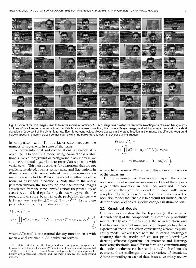
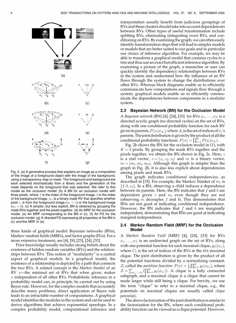
The use of probability models in vision applications is, ofcourse, extensive. Here, we introduce a model that is simpleenough to study in detail here, but also correctly accountsfor an important effect in vision: occlusion. Fig. 1 illustratesthe training data. The goal of the model is to separate thefive foreground objects and the seven background scenes inthese images. This is an important problem in vision thathas broad applicability. For example, by identifying whichpixels belong to the background, it is possible to improvethe performance of a foreground object classifier sinceerrors made by noise in the background will be avoided.

The occlusion model explains an input image, with pixelintensities z1; . . . ; zK , as a composition of a foreground imageand a background image (cf., [1]) and each of these images isselected froma libraryofJ possible images (amixturemodel).Although separate libraries can be used for the foregroundand background, for notational simplicity, we assume theyshare a common image library. The generative process isillustrated in Fig. 2a. To begin with, a foreground image israndomly selected from the library by choosing the classindex f from the distribution, P ðfÞ. Then, depending on theclass of the foreground, a binary mask m ¼ ðm1; . . . ;mKÞ,mi 2 f0; 1g is randomly chosen.mi ¼ 1 indicates that pixel ziisa foregroundpixel,whereasmi ¼ 0 indicates thatpixelzi isabackground pixel. The distribution over mask RVs dependson the foreground class, since the mask must “cut out” theforeground object. However, given the foreground class, themaskRVsarechosenindependently:P ðmjfÞ ¼

QKi¼1 P ðmijfÞ.

Next, the class of the background, b 2 f1; . . . ; Jg, is randomlychosen from P ðbÞ. Finally, the intensity of the pixels in theimage are selected independently, given the mask, the classof the foreground, and the class of the background:P ðzjm; f; bÞ ¼

QKi¼1 P ðzijmi; f; bÞ. The joint distribution is

given by the following product of distributions:

P ðz;m; f; bÞ ¼

P ðbÞP ðfÞ YKi¼1

P ðmijfÞ! YK

i¼1P ðzijmi; f; bÞ

!:

ð1Þ

In this equation, P ðzijmi; f; bÞ can be further factorized bynoticing that if mi ¼ 0, the class is given by the RV b andif mi ¼ 1 the class is given by the RV f . So, we canwrite P ðzijmi; f; bÞ ¼ P ðzijfÞmiP ðzijbÞ1�mi , where P ðzijfÞand P ðzijbÞ are the distributions over the ith pixel intensitygivenby the foregroundandbackground, respectively. Thesedistributions account for the dependence of the pixelintensity on the mixture index, as well as independentobservation noise. The joint distribution can thus be written:

P ðz;m; f; bÞ ¼

P ðbÞP ðfÞ YKi¼1

P ðmijfÞ! YK

i¼1P ðzijfÞmi

! YKi¼1

P ðzijbÞ1�mi

!:

ð2Þ

2 IEEE TRANSACTIONS ON PATTERN ANALYSIS AND MACHINE INTELLIGENCE, VOL. 27, NO. 9, SEPTEMBER 2005

In comparison with (1), this factorization reduces thenumber of arguments in some of the terms.

For representational and computational efficiency, it isoften useful to specify a model using parametric distribu-tions. Given a foreground or background class index k, weassume zi is equal to �ki plus zero-mean Gaussian noise withvariance ki. This noise accounts for distortions that are notexplicitly modeled, such as sensor noise and fluctuations inillumination. If aGaussianmodel of these noise sources is tooinaccurate, extra hiddenRVscanbe added tobettermodel thenoise, as described in Section 3. Note that in the aboveparameterization, the foreground and background imagesare selected from the same library.1 Denote the probability ofclass k by �k and let the probability thatmi ¼ 1, given that theforeground class is f , be �fi. Since the probability thatmi ¼ 0is 1� �fi, we have P ðmijfÞ ¼ �mi

fi ð1� �fiÞ1�mi . Using these

parametric forms, the joint distribution is

P ðz;m; f; bÞ ¼

�b�f

YKi¼1

�mi

fi ð1� �fiÞ1�miNðzi;�fi; fiÞmiNðzi;�bi; biÞ1�mi

!;

ð3Þ

where Nðz;�; Þ is the normal density function on z withmean � and variance . An equivalent form is

P ðz;m; f; bÞ ¼

�b�f

YKi¼1

�mi

fi ð1� �fiÞ1�miNðzi;mi�fi

þ ð1�miÞ�bi;mi fi þ ð1�miÞ biÞ!;

where, here the mask RVs “screen” the mean and varianceof the Gaussians.

In the remainder of this review paper, the aboveocclusion model is used as an example. One of the appealsof generative models is in their modularity and the easewith which they can be extended to cope with morecomplex data. In Section 3, we describe extensions of theocclusion model that enable it to account for motion, objectdeformations, and object-specific changes in illumination.

2.2 Graphical Models

Graphical models describe the topology (in the sense ofdependencies) of the components of a complex probabilitymodel, clarify assumptions about the representation, andlead to algorithms that make use of the topology to achieveexponential speed-ups. When constructing a complex prob-ability model, we are faced with the following challenges:ensuring that the model reflects our prior knowledge;deriving efficient algorithms for inference and learning,translating themodel to a different form, and communicatingthe model to other researchers and users. Graphical modelsovercome these challenges in a wide variety of situations.After commenting on each of these issues, we briefly review

FREY AND JOJIC: A COMPARISON OF ALGORITHMS FOR INFERENCE AND LEARNING IN PROBABILISTIC GRAPHICAL MODELS 3

Fig. 1. Some of the 300 images used to train the model in Section 2.1. Each image was created by randomly selecting one of seven backgroundsand one of five foreground objects from the Yale face database, combining them into a 2-layer image, and adding normal noise with standarddeviation of 2 percent of the dynamic range. Each foreground object always appears in the same location in the image, but different foregroundobjects appear in different places so that each pixel in the background is seen in several training images.

1. If it is desirable that the foreground and background images comefrom separate libraries, the class RVs f and b can be constrained, e.g., so thatf 2 f1; . . . ; ng, b 2 fnþ 1; . . . ; nþ lg, in which case, the first n images in thelibrary are foreground images and the next l images are backgroundimages.

three kinds of graphical model: Bayesian networks (BNs),Markov random fields (MRFs), and factor graphs (FGs). For amore extensive treatment, see [4], [9], [23], [24], [33].

Prior knowledge usually includes strong beliefs about theexistence of hidden random variables (RVs) and the relation-ships between RVs. This notion of “modularity” is a centralaspect of graphical models. In a graphical model, theexistence of a relationship is depicted by a path that connectsthe two RVs. A related concept is the Markov blanket of anRV x—the minimal set of RVs that when given, makesx independent of all other RVs. Probabilistic inference in aprobability model can, in principle, be carried out by usingBayes rule. However, for the complex models that accuratelydescribe many problems, direct application of Bayes ruleleads to an intractable number of computations. A graphicalmodel identifies themodules in the systemand can beused toderive algorithms that achieve exponential speedups. In acomplex probability model, computational inference and

interpretation usually benefit from judicious groupings ofRVsand these clusters should take into accountdependenciesbetween RVs. Other types of useful transformation includesplitting RVs, eliminating (integrating over) RVs, and con-ditioningonRVs. Byexamining thegraph,we canoften easilyidentify transformation steps thatwill lead to simplermodelsor models that are better suited to our goals and in particularour choice of inference algorithm. For example, we may beable to transform a graphical model that contains cycles to atree and thususe anexact but efficient inference algorithm.Byexamining a picture of the graph, a researcher or user canquickly identify the dependency relationships between RVsin the system and understand how the influence of an RVflows through the system to change the distributions overother RVs. Whereas block diagrams enable us to efficientlycommunicate how computations and signals flow through asystem, graphical models enable us to efficiently commu-nicate the dependencies between components in a modularsystem.

2.3 Bayesian Network (BN) for the Occlusion Model

A Bayesian network (BN) [4], [24], [33] for RVs x1; . . . ; xN is adirected acyclic graph (no directed cycles) on the set of RVs,along with one conditional probability function for each RVgiven itsparents,P ðxijxAi

Þ,whereAi is the setof indicesofxi’sparents.The jointdistribution isgivenby theproductof all theconditional probability functions: P ðxÞ ¼

QNi¼1 P ðxijxAi

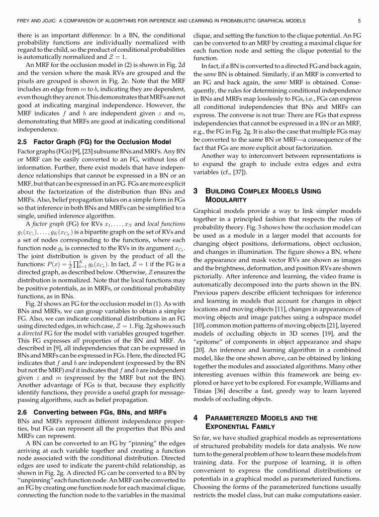
Þ.Fig. 2b shows the BN for the occlusion model in (1), with

K ¼ 3 pixels. By grouping the mask RVs together and thepixels together, we obtain the BN shown in Fig. 2c. Here, zis a real vector, z ¼ ðz1; z2; z3Þ and m is a binary vector,m ¼ ðm1;m2;m3Þ. Although this graph is simpler than thegraph in Fig. 2b, it is also less explicit about dependenciesamong pixels and mask RVs.

The graph indicates conditional independencies, asdescribed in [33]. For example, the Markov blanket of m1 isff; b; z1g. In a BN, observing a child induces a dependencebetween its parents. Here, the BN indicates that f and b aredependent given z and m, even though they are not(observing m decouples f and b). This demonstrates thatBNs are not good at indicating conditional independence.However, the BN indicates that f and b are marginallyindependent, demonstrating that BNs are good at indicatingmarginal independence.

2.4 Markov Random Field (MRF) for the OcclusionModel

A Markov Random Field (MRF) [4], [24], [33] for RVs

x1; . . . ; xN is an undirected graph on the set of RVs, along

with one potential function for each maximal clique, gkðxCkÞ,where Ck is the set of indices of the RVs in the kth maximal

clique. The joint distribution is given by the product of all

the potential functions divided by a normalizing constant,

Z, called the partition function: P ðxÞ ¼ 1ZQK

k¼1 gkðxCkÞ, where

Z ¼P

x1;...;xNðQK

k¼1 gkðxCkÞÞ. A clique is a fully connected

subgraph, and a maximal clique is a clique that cannot be

made larger while still being a clique. For brevity, we use

the term “clique” to refer to a maximal clique, e.g., the

potentials on maximal cliques are usually called clique

potentials.Theabove factorizationof the jointdistribution is similar to

the factorization for the BN, where each conditional prob-ability function can be viewed as a clique potential. However,


Fig. 2. (a) A generative process that explains an image as a compositionof the image of a foreground object with the image of the background,using a transparency map or mask. The foreground and background areeach selected stochastically from a library and the generation of themask depends on the foreground that was selected. We refer to thismodel as the occlusion model. (b) A BN for an occlusion model withthree pixels, where f is the index of the foreground image, b is the indexof the background image,mi is a binary mask RV that specifies whetherpixel zi is from the foreground image (mi ¼ 1) or the background image(mi ¼ 0). (c) A simpler, but less explicit, BN is obtained by grouping themask RVs together and the pixels together. (d) An MRF for the occlusionmodel. (e) An MRF corresponding to the BN in (c). (f) An FG for theocclusion model. (g) A directed FG expressing all properties of the BN in(c) and the MRF in (e).

there is an important difference: In a BN, the conditionalprobability functions are individually normalized withregard to the child, so the product of conditional probabilitiesis automatically normalized andZ ¼ 1.

An MRF for the occlusion model in (2) is shown in Fig. 2d

and the version where the mask RVs are grouped and the

pixels are grouped is shown in Fig. 2e. Note that the MRF

includes an edge fromm to b, indicating they are dependent,

eventhoughtheyarenot.Thisdemonstrates thatMRFsarenot

good at indicating marginal independence. However, the

MRF indicates f and b are independent given z and m,

demonstrating that MRFs are good at indicating conditional

independence.

2.5 Factor Graph (FG) for the Occlusion Model

Factor graphs (FGs) [9], [23] subsumeBNsandMRFs.AnyBN

or MRF can be easily converted to an FG, without loss of

information. Further, there exist models that have indepen-

dence relationships that cannot be expressed in a BN or an

MRF,but that canbeexpressed inanFG.FGsaremore explicit

about the factorization of the distribution than BNs and

MRFs. Also, belief propagation takes on a simple form in FGs

so that inference in both BNs andMRFs can be simplified to a

single, unified inference algorithm.

A factor graph (FG) for RVs x1; . . . ; xN and local functions

g1ðxC1Þ; . . . ; gKðxCK Þ is a bipartite graph on the set of RVs and

a set of nodes corresponding to the functions, where each

function node gk is connected to the RVs in its argument xCk .

The joint distribution is given by the product of all the

functions: P ðxÞ ¼ 1ZQK

k¼1 gkðxCkÞ. In fact, Z ¼ 1 if the FG is a

directed graph, as described below.Otherwise,Z ensures the

distribution is normalized. Note that the local functions may

be positive potentials, as in MRFs, or conditional probability

functions, as in BNs.Fig. 2f shows an FG for the occlusionmodel in (1). As with

BNs and MRFs, we can group variables to obtain a simplerFG. Also, we can indicate conditional distributions in an FGusingdirected edges, inwhich case,Z ¼ 1. Fig. 2g shows sucha directed FG for the model with variables grouped together.This FG expresses all properties of the BN and MRF. Asdescribed in [9], all independencies that can be expressed inBNs andMRFs canbe expressed inFGs.Here, thedirected FGindicates that f and b are independent (expressed by the BNbut not theMRF) and it indicates that f and b are independentgiven z and m (expressed by the MRF but not the BN).Another advantage of FGs is that, because they explicitlyidentify functions, they provide a useful graph for message-passing algorithms, such as belief propagation.

2.6 Converting between FGs, BNs, and MRFs

BNs and MRFs represent different independence proper-ties, but FGs can represent all the properties that BNs andMRFs can represent.

A BN can be converted to an FG by “pinning” the edgesarriving at each variable together and creating a functionnode associated with the conditional distribution. Directededges are used to indicate the parent-child relationship, asshown in Fig. 2g. A directed FG can be converted to a BN by“unpinning”each functionnode.AnMRFcanbeconverted toan FG by creating one function node for eachmaximal clique,connecting the function node to the variables in the maximal

clique, and setting the function to the clique potential. An FGcan be converted to an MRF by creating a maximal clique foreach function node and setting the clique potential to thefunction.

In fact, if aBN is converted to adirectedFGandbackagain,

the same BN is obtained. Similarly, if an MRF is converted to

an FG and back again, the same MRF is obtained. Conse-

quently, the rules for determining conditional independence

in BNs andMRFs map losslessly to FGs, i.e., FGs can express

all conditional independencies that BNs and MRFs can

express. The converse is not true: There are FGs that express

independencies that cannot be expressed in a BN or anMRF,

e.g., the FG in Fig. 2g. It is also the case thatmultiple FGsmay

be converted to the same BN or MRF—a consequence of the

fact that FGs are more explicit about factorization.

Another way to interconvert between representations is

to expand the graph to include extra edges and extra

variables (cf., [37]).

3 BUILDING COMPLEX MODELS USING

MODULARITY

Graphical models provide a way to link simpler models

together in a principled fashion that respects the rules of

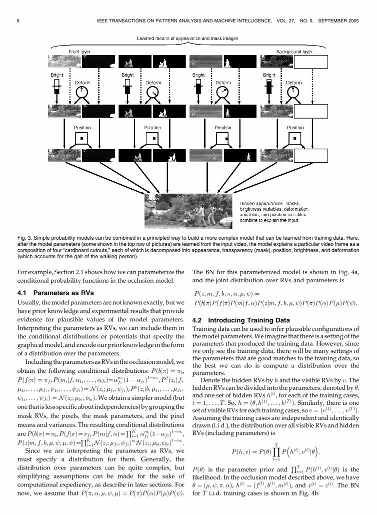
probability theory. Fig. 3 shows how the occlusionmodel can

be used as a module in a larger model that accounts for

changing object positions, deformations, object occlusion,

and changes in illumination. The figure shows a BN, where

the appearance and mask vector RVs are shown as images

and the brightness, deformation, andposition RVs are shown

pictorially. After inference and learning, the video frame is

automatically decomposed into the parts shown in the BN.

Previous papers describe efficient techniques for inference

and learning in models that account for changes in object

locations andmoving objects [11], changes in appearances of

moving objects and image patches using a subspace model

[10], commonmotion patterns ofmoving objects [21], layered

models of occluding objects in 3D scenes [19], and the

“epitome” of components in object appearance and shape

[20]. An inference and learning algorithm in a combined

model, like the one shown above, can be obtained by linking

together the modules and associated algorithms. Many other

interesting avenues within this framework are being ex-

plored or have yet to be explored. For example,Williams and

Titsias [36] describe a fast, greedy way to learn layered

models of occluding objects.

4 PARAMETERIZED MODELS AND THE

EXPONENTIAL FAMILY

So far, we have studied graphical models as representations

of structured probability models for data analysis. We now

turn to thegeneral problemofhow to learn thesemodels from

training data. For the purpose of learning, it is often

convenient to express the conditional distributions or

potentials in a graphical model as parameterized functions.

Choosing the forms of the parameterized functions usually

restricts the model class, but can make computations easier.


For example, Section 2.1 shows howwe can parameterize the

conditional probability functions in the occlusion model.

4.1 Parameters as RVs

Usually, themodel parameters are not known exactly, butwe

have prior knowledge and experimental results that provide

evidence for plausible values of the model parameters.

Interpreting the parameters as RVs, we can include them in

the conditional distributions or potentials that specify the

graphicalmodel, andencodeourprior knowledge in the form

of a distribution over the parameters.

IncludingtheparametersasRVsintheocclusionmodel,we

obtain the following conditional distributions: P ðbj�Þ ¼ �b,P ðf j�Þ ¼ �f ,P ðmijf; �1i; . . . ; �JiÞ¼�mi

fi ð1� �fiÞ1�mi ,Pfðzijf;

�1i; . . . ; �Ji; 1i; . . . ; JiÞ¼ N ðzi;�fi; fiÞ,Pbðzijb; �1i; . . . ; �Ji; 1i; . . . ; JiÞ ¼ N ðzi;�bi; biÞ. We obtain a simplermodel (but

one that is lessspecificabout independencies)bygroupingthe

mask RVs, the pixels, the mask parameters, and the pixel

means and variances. The resulting conditional distributions

areP ðbj�Þ¼�b,P ðf j�Þ¼�f ,P ðmjf; �Þ¼QK

i¼1 �mi

fi ð1��fiÞ1�mi ,

P ðzjm; f; b; �; ; �; Þ¼QK

i¼1Nðzi;�fi; fiÞmiNðzi;�bi; biÞ1�mi .

Since we are interpreting the parameters as RVs, we

must specify a distribution for them. Generally, the

distribution over parameters can be quite complex, but

simplifying assumptions can be made for the sake of

computational expediency, as describe in later sections. For

now, we assume that P ð�; �; �; ; �Þ ¼ P ð�ÞP ð�ÞP ð�ÞP ð Þ.

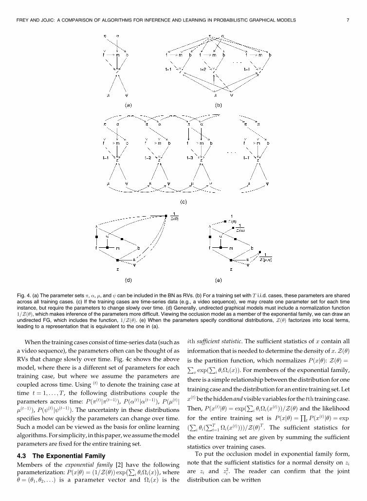
The BN for this parameterized model is shown in Fig. 4a,

and the joint distribution over RVs and parameters is

P ðz;m; f; b; �; �; �; Þ ¼P ðbj�ÞP ðf j�ÞP ðmjf; �ÞP ðzjm; f; b; �; ÞP ð�ÞP ð�ÞP ð�ÞP ð Þ:

4.2 Introducing Training Data

Training data can be used to infer plausible configurations ofthemodelparameters.We imagine that there is a settingof theparameters that produced the training data. However, sincewe only see the training data, there will be many settings ofthe parameters that are good matches to the training data, sothe best we can do is compute a distribution over theparameters.

Denote the hidden RVs by h and the visible RVs by v. ThehiddenRVs can be divided into the parameters, denoted by �,and one set of hidden RVs hðtÞ, for each of the training cases,t ¼ 1; . . . ; T . So, h ¼ ð�; hð1Þ; . . . ; hðT ÞÞ. Similarly, there is oneset of visibleRVs for each training cases, so v ¼ ðvð1Þ; . . . ; vðT ÞÞ.Assuming the training cases are independent and identicallydrawn (i.i.d.), the distribution over all visible RVs andhiddenRVs (including parameters) is

P ðh; vÞ ¼ P ð�ÞYTt¼1

P hðtÞ; vðtÞj��

:

P ð�Þ is the parameter prior andQT

t¼1 P ðhðtÞ; vðtÞj�Þ is thelikelihood. In the occlusion model described above, we have� ¼ ð�; ; �; �Þ, hðtÞ ¼ ðf ðtÞ; bðtÞ;mðtÞÞ, and vðtÞ ¼ zðtÞ. The BNfor T i.i.d. training cases is shown in Fig. 4b.


Fig. 3. Simple probability models can be combined in a principled way to build a more complex model that can be learned from training data. Here,after the model parameters (some shown in the top row of pictures) are learned from the input video, the model explains a particular video frame as acomposition of four “cardboard cutouts,” each of which is decomposed into appearance, transparency (mask), position, brightness, and deformation(which accounts for the gait of the walking person).

When the training cases consist of time-series data (such as

a video sequence), the parameters often can be thought of as

RVs that change slowly over time. Fig. 4c shows the above

model, where there is a different set of parameters for each

training case, but where we assume the parameters are

coupled across time. Using ðtÞ to denote the training case at

time t ¼ 1; . . . ; T , the following distributions couple the

parameters across time: P ð�ðtÞj�ðt�1ÞÞ, P ð�ðtÞj�ðt�1ÞÞ, P ð�ðtÞj�ðt�1ÞÞ, P ð ðtÞj ðt�1ÞÞ. The uncertainty in these distributions

specifies how quickly the parameters can change over time.

Such a model can be viewed as the basis for online learning

algorithms.Forsimplicity, in thispaper,weassumethemodel

parameters are fixed for the entire training set.

4.3 The Exponential Family

Members of the exponential family [2] have the followingparameterization: P ðxj�Þ ¼ ð1=Zð�ÞÞ exp

�Pi �i�iðxÞ

�, where

� ¼ ð�1; �2; . . .Þ is a parameter vector and �iðxÞ is the

ith sufficient statistic. The sufficient statistics of x contain all

information that is needed to determine the density of x.Zð�Þis the partition function, which normalizes P ðxj�Þ: Zð�Þ ¼P

x expðP

i �i�iðxÞÞ. For members of the exponential family,

there is a simple relationship between the distribution for one

training case and thedistribution for an entire training set. Let

xðtÞ be thehidden andvisiblevariables for the tth training case.

Then, P ðxðtÞj�Þ ¼ expðP

i �i�iðxðtÞÞÞ=Zð�Þ and the likelihood

for the entire training set is P ðxj�Þ ¼Q

t P ðxðtÞj�Þ ¼ exp

ðP

i �iðPT

t¼1 �iðxðtÞÞÞÞ=Zð�ÞT . The sufficient statistics for

the entire training set are given by summing the sufficient

statistics over training cases.To put the occlusion model in exponential family form,

note that the sufficient statistics for a normal density on zi

are zi and z2i . The reader can confirm that the joint

distribution can be written


Fig. 4. (a) The parameter sets �, �, �, and can be included in the BN as RVs. (b) For a training set with T i.i.d. cases, these parameters are sharedacross all training cases. (c) If the training cases are time-series data (e.g., a video sequence), we may create one parameter set for each timeinstance, but require the parameters to change slowly over time. (d) Generally, undirected graphical models must include a normalization function1=Zð�Þ, which makes inference of the parameters more difficult. Viewing the occlusion model as a member of the exponential family, we can draw anundirected FG, which includes the function, 1=Zð�Þ. (e) When the parameters specify conditional distributions, Zð�Þ factorizes into local terms,leading to a representation that is equivalent to the one in (a).

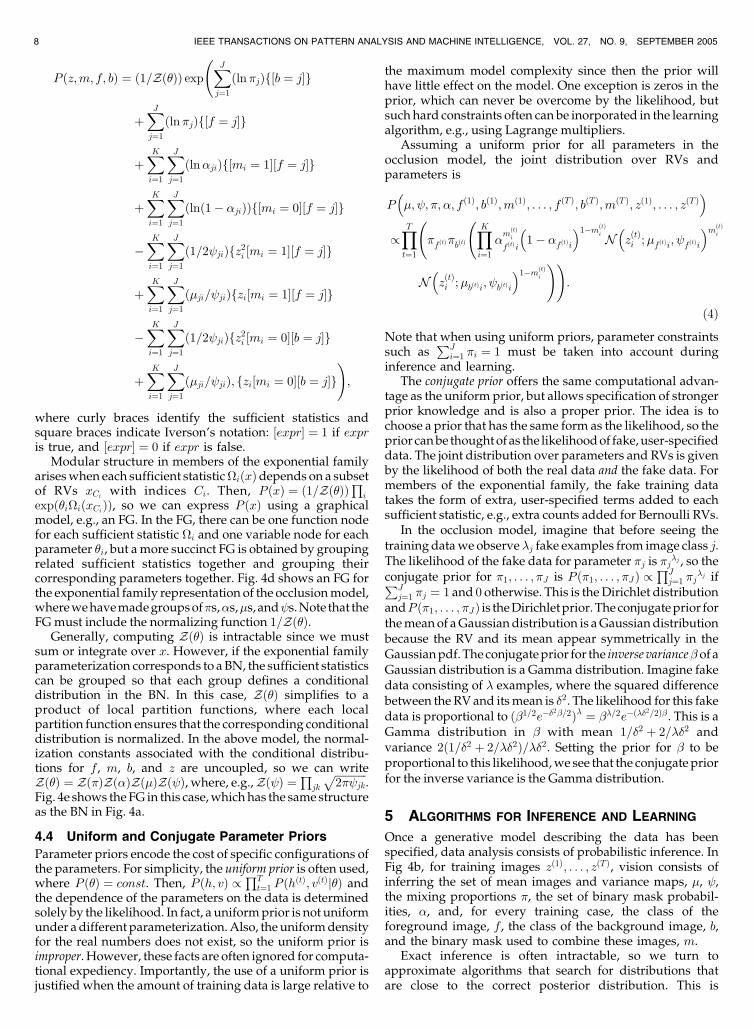
P ðz;m; f; bÞ ¼ ð1=Zð�ÞÞ exp XJ

j¼1ðln�jÞf½b ¼ j�g

þXJj¼1ðln�jÞf½f ¼ j�g

þXKi¼1

XJj¼1ðln�jiÞf½mi ¼ 1�½f ¼ j�g

þXKi¼1

XJj¼1ðlnð1� �jiÞÞf½mi ¼ 0�½f ¼ j�g

�XKi¼1

XJj¼1ð1=2 jiÞfz2i ½mi ¼ 1�½f ¼ j�g

þXKi¼1

XJj¼1ð�ji= jiÞfzi½mi ¼ 1�½f ¼ j�g

�XKi¼1

XJj¼1ð1=2 jiÞfz2i ½mi ¼ 0�½b ¼ j�g

þXKi¼1

XJj¼1ð�ji= jiÞ; fzi½mi ¼ 0�½b ¼ j�g

!;

where curly braces identify the sufficient statistics andsquare braces indicate Iverson’s notation: ½expr� ¼ 1 if expris true, and ½expr� ¼ 0 if expr is false.

Modular structure in members of the exponential familyariseswhen each sufficient statistic�iðxÞdepends on a subsetof RVs xCi with indices Ci. Then, P ðxÞ ¼ ð1=Zð�ÞÞ

Qi

expð�i�iðxCiÞÞ, so we can express P ðxÞ using a graphicalmodel, e.g., an FG. In the FG, there can be one function nodefor each sufficient statistic �i and one variable node for eachparameter �i, but amore succinct FG is obtained by groupingrelated sufficient statistics together and grouping theircorresponding parameters together. Fig. 4d shows an FG forthe exponential family representation of the occlusionmodel,wherewehavemadegroupsof�s,�s,�s, and s.Note that theFGmust include the normalizing function 1=Zð�Þ.

Generally, computing Zð�Þ is intractable since we mustsum or integrate over x. However, if the exponential familyparameterization corresponds to aBN, the sufficient statisticscan be grouped so that each group defines a conditionaldistribution in the BN. In this case, Zð�Þ simplifies to aproduct of local partition functions, where each localpartition function ensures that the corresponding conditionaldistribution is normalized. In the above model, the normal-ization constants associated with the conditional distribu-tions for f , m, b, and z are uncoupled, so we can writeZð�Þ ¼ Zð�ÞZð�ÞZð�ÞZð Þ, where, e.g.,Zð Þ ¼

Qjk

ffiffiffiffiffiffiffiffiffiffiffiffi2� jk

p.

Fig. 4e shows theFG in this case,whichhas the same structureas the BN in Fig. 4a.

4.4 Uniform and Conjugate Parameter Priors

Parameter priors encode the cost of specific configurations ofthe parameters. For simplicity, the uniform prior is often used,where P ð�Þ ¼ const. Then, P ðh; vÞ /

QTt¼1 P ðhðtÞ; vðtÞj�Þ and

the dependence of the parameters on the data is determinedsolely by the likelihood. In fact, a uniformprior is not uniformunder adifferent parameterization.Also, theuniformdensityfor the real numbers does not exist, so the uniform prior isimproper. However, these facts are often ignored for computa-tional expediency. Importantly, the use of a uniform prior isjustified when the amount of training data is large relative to

the maximum model complexity since then the prior willhave little effect on the model. One exception is zeros in theprior, which can never be overcome by the likelihood, butsuchhard constraints often can be inorporated in the learningalgorithm, e.g., using Lagrange multipliers.

Assuming a uniform prior for all parameters in theocclusion model, the joint distribution over RVs andparameters is

P �; ; �; �; f ð1Þ; bð1Þ;mð1Þ; . . . ; fðT Þ; bðT Þ;mðT Þ; zð1Þ; . . . ; zðT Þ� �

/YTt¼1

�fðtÞ�bðtÞ

YKi¼1

�mðtÞi

fðtÞi1� �f ðtÞi� �1�mðtÞi N z

ðtÞi ;�fðtÞi; fðtÞi

� �mðtÞi

N zðtÞi ;�bðtÞi; bðtÞi

� �1�mðtÞi !!:

ð4Þ

Note that when using uniform priors, parameter constraintssuch as

PJi¼1 �i ¼ 1 must be taken into account during

inference and learning.The conjugate prior offers the same computational advan-

tage as the uniform prior, but allows specification of strongerprior knowledge and is also a proper prior. The idea is tochoose a prior that has the same form as the likelihood, so theprior canbe thoughtofas the likelihoodof fake,user-specifieddata. The joint distribution over parameters and RVs is givenby the likelihood of both the real data and the fake data. Formembers of the exponential family, the fake training datatakes the form of extra, user-specified terms added to eachsufficient statistic, e.g., extra counts added for Bernoulli RVs.

In the occlusion model, imagine that before seeing thetraining datawe observe �j fake examples from image class j.The likelihood of the fake data for parameter �j is �j

�j , so theconjugate prior for �1; . . . ; �J is P ð�1; . . . ; �JÞ /

QJj¼1 �j

�j ifPJj¼1 �j ¼ 1 and 0 otherwise. This is theDirichlet distribution

andP ð�1; . . . ; �JÞ is theDirichletprior.Theconjugateprior forthemeanof aGaussiandistribution is aGaussiandistributionbecause the RV and its mean appear symmetrically in theGaussianpdf.The conjugateprior for the inverse variance� of aGaussian distribution is a Gamma distribution. Imagine fakedata consisting of � examples, where the squared differencebetween the RV and itsmean is �2. The likelihood for this fakedata is proportional to ð�1=2e��2�=2Þ� ¼ ��=2e�ð��2=2Þ�. This is aGamma distribution in � with mean 1=�2 þ 2=��2 andvariance 2ð1=�2 þ 2=��2Þ=��2. Setting the prior for � to beproportional to this likelihood,we see that the conjugatepriorfor the inverse variance is the Gamma distribution.

5 ALGORITHMS FOR INFERENCE AND LEARNING

Once a generative model describing the data has beenspecified, data analysis consists of probabilistic inference. InFig 4b, for training images zð1Þ; . . . ; zðT Þ, vision consists ofinferring the set of mean images and variance maps, �, ,the mixing proportions �, the set of binary mask probabil-ities, �, and, for every training case, the class of theforeground image, f , the class of the background image, b,and the binary mask used to combine these images, m.

Exact inference is often intractable, so we turn toapproximate algorithms that search for distributions thatare close to the correct posterior distribution. This is


accomplished by minimizing pseudodistances on distribu-tions, called “free energies.” (For an alternative view, see[34].) It is interesting that, in the 1800s, Helmholtz was oneof the first researchers to propose that vision is inference ina generative model and that nature seeks correct probabilitydistributions in physical systems by minimizing freeenergy. Although there is no record that Helmholtz sawthat the brain might perform vision by minimizing a freeenergy, we can’t help but wonder if he pondered this.

Viewing parameters as RVs, inference algorithms for RVsand parameters alike make use of the conditional indepen-dencies in the graphical model. It is possible to describegraph-based propagation algorithms for updating distribu-tions over parameters [15]. It is often important to treatparameters and RVs differently during inference. Whereaseach RV plays a role in a single training case, the parametersare shared acrossmany training cases. So, the parameters areimpacted by more evidence than RVs and are often pinneddown more tightly by the data. This observation becomesrelevant when we study approximate inference techniquesthat obtain point estimates of the parameters, such as theexpectation maximization algorithm [6].

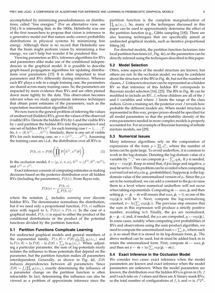
Wenow turn to the general problemof inferring the valuesof unobserved (hidden) RVs, given the values of the observed(visible) RVs.Denote the hiddenRVs by h and the visible RVsby v and partition the hidden RVs into the parameters � andone set of hidden RVs hðtÞ, for each training case t ¼ 1; . . . ; T .So, h ¼ ð�; hð1Þ; . . . ; hðT ÞÞ. Similarly, there is one set of visibleRVs for each training case, so v ¼ ðvð1Þ; . . . ; vðT ÞÞ. Assumingthe training cases are i.i.d., the distribution over all RVs is

P ðh; vÞ ¼ P ð�Þ YTt¼1

P hðtÞ; vðtÞj�� !

: ð5Þ

In the occlusion model, � ¼ ð�; ; �; �Þ, hðtÞ ¼ ðf ðtÞ; bðtÞ;mðtÞÞ,and vðtÞ ¼ zðtÞ.

Exact inference consists of computing estimates ormakingdecisions based on the posterior distribution over all hiddenRVs (including the parameters), P ðhjvÞ. From Bayes rule,

P ðhjvÞ ¼ P ðh; vÞRh P ðh; vÞ

;

where the notationRh includes summing over discrete

hidden RVs. The denominator normalizes the distribution,but if we need only a proportional function, P ðh; vÞ sufficessince with regard to h, P ðhjvÞ / P ðh; vÞ. In the case of agraphical model, P ðh; vÞ is equal to either the product of theconditional distributions or the product of the potentialfunctions divided by the partition function.

5.1 Partition Functions Complicate Learning

For undirected graphical models and general members ofthe exponential family, P ðx; �Þ ¼ P ð�Þ 1

Zð�ÞQ

k gkðxCkÞ andlnP ðx; �Þ ¼ lnP ð�Þ � lnZð�Þ þ

Pk ln gkðxCkÞ. When adjust-

ing a particular parameter, the sum of log-potentials nicelyisolates the influence to those potentials that depend on theparameter, but the partition function makes all parametersinterdependent. Generally, as shown in Fig. 4d, Zð�Þinduces dependencies between all parameters. SinceZð�Þ ¼

RxðQ

k gkðxCkÞ, exactly determining the influence ofa parameter change on the partition function is oftenintractable. In fact, determining this influence can also beviewed as a problem of approximate inference since the

partition function is the complete marginalization ofQk gkðxCkÞ. So, many of the techniques discussed in this

paper can be used to approximately determine the effect ofthe partition function (e.g., Gibbs sampling [18]). There arealso learning techniques that are specifically aimed atundirected graphical models, such as iterative proportionalfitting [4].

For directed models, the partition function factorizes intolocal partition functions (cf., Fig. 4e), so the parameters can bedirectly inferredusing the techniques described in this paper.

5.2 Model Selection

Often, some aspects of the model structure are known, butothers are not. In the occlusion model, we may be confidentabout the structure of the BN in Fig. 4b, but not the number ofclasses, J . Unknown structure can be represented as a hiddenRV so that inference of this hidden RV corresponds toBayesian model selection [16], [25]. The BN in Fig. 4b can bemodified to include an RV, J , whose children are all of the fand b variables and where J limits the range of the classindices. Given a training set, the posterior over J reveals howprobable the different models are. When model structure isrepresented in thisway, proper priors should be specified forall model parameters so that the probability density of theextra parameters needed inmore complexmodels is properlyaccounted for. For an example of Bayesian learning of infinitemixture models, see [29].

5.3 Numerical Issues

Many inference algorithms rely on the computation ofexpressions of the form p ¼

Qj a

qjj , where the number of

terms can be quite large. To avoid underflow, it is common towork in the log-domain. Denoting the log-domain value of avariable by “~,” we can compute ~pp

Pj qj~aaj. If p is needed,

set p expð~ppÞ. Keep inmind that, if ~pp is large and negative, pmaybeset to0. Thisproblemcanbeavoidedwhencomputinganormalized set ofpis (e.g., probabilities). Suppose ~ppi is the log-domain value of the unnormalized version of pi. Since the pisare to be normalized, we can add a constant to the ~ppis to raisethem to a level where numerical underflow will not occurwhen taking exponentials. Computing ~mm maxi ~ppi and thensetting ~ppi ~ppi � ~mmwill ensure thatmaxi ~ppi ¼ 0, so one of theexpð~ppiÞs will be 1. Next, compute the log-normalizingconstant, ~cc lnð

Pi expð~ppiÞÞ. The previous step ensures that

the sum in this expression will produce a strictly positivenumber, avoiding ln 0. Finally, the ~ppis are normalized,~ppi ~ppi�~cc, and, if needed, the pis are computed, pi expð~ppiÞ.In some cases, notably when computing joint probabilities ofRVs and observations using the sum-product algorithm, weneed to compute theunnormalized sum s¼

Pi pi, where each

pi is so small that it is stored in its log-domain form, ~ppi. Theabove method can be used, but ~mm must be added back in toretain the unnormalized form. First, compute ~mm maxi ~ppiand then set ~ss ~mmþ lnð

Pi expð~ppi � ~mmÞÞ.

5.4 Exact Inference in the Occlusion Model

We consider two cases: exact inference when the modelparameters are known and exact inference when the modelparameters are unknown. When the model parameters areknown, the distribution over the hidden RVs is given in (3). fand b each take on J values and there areK binarymask RVs,so the total number of configurations of f , b, and m is J22K .


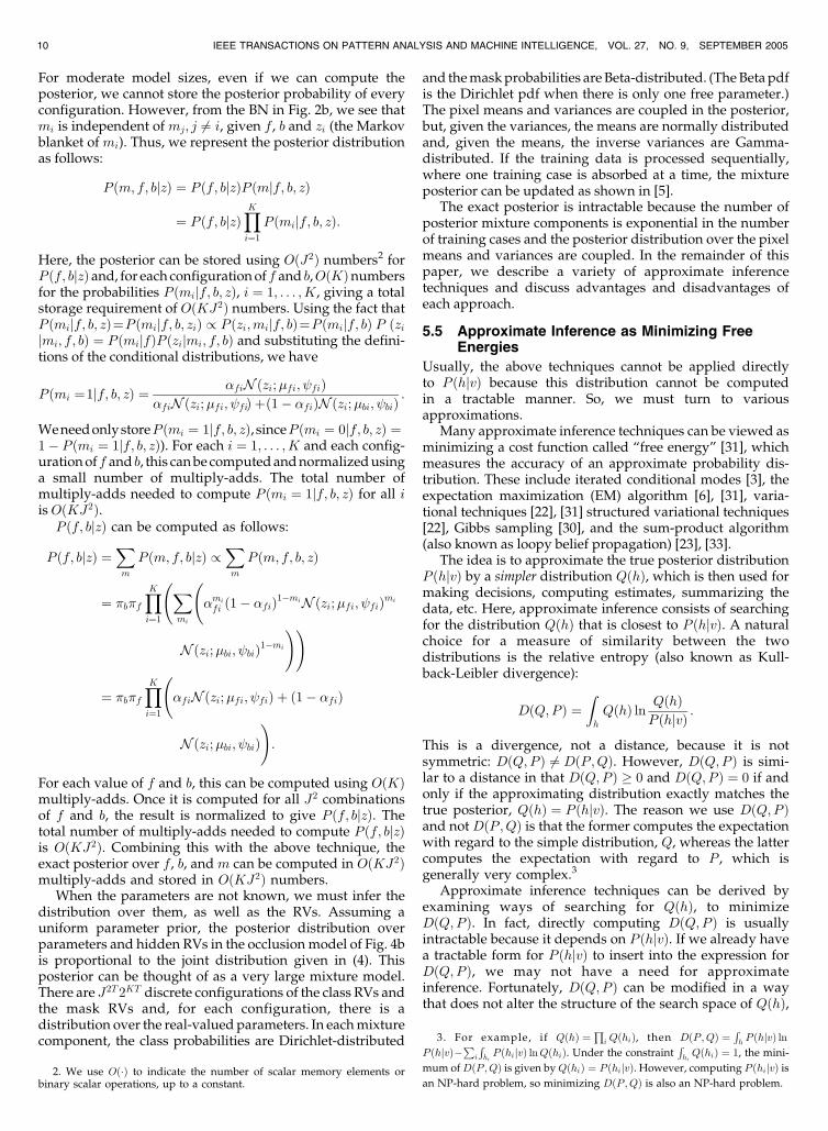
For moderate model sizes, even if we can compute theposterior, we cannot store the posterior probability of everyconfiguration. However, from the BN in Fig. 2b, we see thatmi is independent ofmj; j 6¼ i, given f , b and zi (the Markovblanket ofmi). Thus, we represent the posterior distributionas follows:

P ðm; f; bjzÞ ¼ P ðf; bjzÞP ðmjf; b; zÞ

¼ P ðf; bjzÞYKi¼1

P ðmijf; b; zÞ:

Here, the posterior can be stored using OðJ2Þ numbers2 forP ðf; bjzÞand, for each configurationof f and b,OðKÞnumbersfor the probabilities P ðmijf; b; zÞ, i ¼ 1; . . . ; K, giving a totalstorage requirement of OðKJ2Þ numbers. Using the fact thatP ðmijf; b; zÞ¼P ðmijf; b; ziÞ / P ðzi;mijf; bÞ¼P ðmijf; bÞ P ðzijmi; f; bÞ ¼ P ðmijfÞP ðzijmi; f; bÞ and substituting the defini-tions of the conditional distributions, we have

P ðmi ¼1jf; b; zÞ ¼ �fiNðzi;�fi; fiÞ�fiNðzi;�fi; fiÞ þð1� �fiÞN ðzi;�bi; biÞ

:

WeneedonlystoreP ðmi ¼ 1jf; b; zÞ, sinceP ðmi ¼ 0jf; b; zÞ ¼1� P ðmi ¼ 1jf; b; zÞ). For each i ¼ 1; . . . ; K and each config-urationoff and b, this canbecomputedandnormalizedusinga small number of multiply-adds. The total number ofmultiply-adds needed to compute P ðmi ¼ 1jf; b; zÞ for all iisOðKJ2Þ.P ðf; bjzÞ can be computed as follows:

P ðf; bjzÞ ¼Xm

P ðm; f; bjzÞ /Xm

P ðm; f; b; zÞ

¼ �b�fYKi¼1

Xmi

�mi

fi ð1� �fiÞ1�miNðzi;�fi; fiÞmi

Nðzi;�bi; biÞ1�mi

!!

¼ �b�fYKi¼1

�fiNðzi;�fi; fiÞ þ ð1� �fiÞ

N ðzi;�bi; biÞ!:

For each value of f and b, this can be computed using OðKÞmultiply-adds. Once it is computed for all J2 combinationsof f and b, the result is normalized to give P ðf; bjzÞ. Thetotal number of multiply-adds needed to compute P ðf; bjzÞis OðKJ2Þ. Combining this with the above technique, theexact posterior over f , b, andm can be computed in OðKJ2Þmultiply-adds and stored in OðKJ2Þ numbers.

When the parameters are not known, we must infer thedistribution over them, as well as the RVs. Assuming auniform parameter prior, the posterior distribution overparameters and hidden RVs in the occlusion model of Fig. 4bis proportional to the joint distribution given in (4). Thisposterior can be thought of as a very large mixture model.There are J2T2KT discrete configurations of the class RVs andthe mask RVs and, for each configuration, there is adistribution over the real-valued parameters. In eachmixturecomponent, the class probabilities are Dirichlet-distributed

and themaskprobabilities areBeta-distributed. (TheBetapdfis the Dirichlet pdf when there is only one free parameter.)The pixel means and variances are coupled in the posterior,but, given the variances, the means are normally distributedand, given the means, the inverse variances are Gamma-distributed. If the training data is processed sequentially,where one training case is absorbed at a time, the mixtureposterior can be updated as shown in [5].

The exact posterior is intractable because the number ofposterior mixture components is exponential in the numberof training cases and the posterior distribution over the pixelmeans and variances are coupled. In the remainder of thispaper, we describe a variety of approximate inferencetechniques and discuss advantages and disadvantages ofeach approach.

5.5 Approximate Inference as Minimizing FreeEnergies

Usually, the above techniques cannot be applied directlyto P ðhjvÞ because this distribution cannot be computedin a tractable manner. So, we must turn to variousapproximations.

Many approximate inference techniques can be viewed asminimizing a cost function called “free energy” [31], whichmeasures the accuracy of an approximate probability dis-tribution. These include iterated conditional modes [3], theexpectation maximization (EM) algorithm [6], [31], varia-tional techniques [22], [31] structured variational techniques[22], Gibbs sampling [30], and the sum-product algorithm(also known as loopy belief propagation) [23], [33].

The idea is to approximate the true posterior distributionP ðhjvÞ by a simpler distribution QðhÞ, which is then used formaking decisions, computing estimates, summarizing thedata, etc. Here, approximate inference consists of searchingfor the distribution QðhÞ that is closest to P ðhjvÞ. A naturalchoice for a measure of similarity between the twodistributions is the relative entropy (also known as Kull-back-Leibler divergence):

DðQ;P Þ ¼Zh

QðhÞ ln QðhÞP ðhjvÞ :

This is a divergence, not a distance, because it is notsymmetric: DðQ;P Þ 6¼ DðP;QÞ. However, DðQ;P Þ is simi-lar to a distance in that DðQ;P Þ � 0 and DðQ;P Þ ¼ 0 if andonly if the approximating distribution exactly matches thetrue posterior, QðhÞ ¼ P ðhjvÞ. The reason we use DðQ;P Þand notDðP;QÞ is that the former computes the expectationwith regard to the simple distribution, Q, whereas the lattercomputes the expectation with regard to P , which isgenerally very complex.3

Approximate inference techniques can be derived byexamining ways of searching for QðhÞ, to minimizeDðQ;P Þ. In fact, directly computing DðQ;P Þ is usuallyintractable because it depends on P ðhjvÞ. If we already havea tractable form for P ðhjvÞ to insert into the expression forDðQ;P Þ, we may not have a need for approximateinference. Fortunately, DðQ;P Þ can be modified in a waythat does not alter the structure of the search space of QðhÞ,


2. We use Oð�Þ to indicate the number of scalar memory elements orbinary scalar operations, up to a constant.

3. For example, if QðhÞ ¼Q

i QðhiÞ, then DðP;QÞ ¼Rh P ðhjvÞ ln

P ðhjvÞ�P

i

RhiP ðhijvÞ lnQðhiÞ. Under the constraint

RhiQðhiÞ ¼ 1, the mini-

mum ofDðP;QÞ is given byQðhiÞ ¼ P ðhijvÞ. However, computing P ðhijvÞ isan NP-hard problem, so minimizing DðP;QÞ is also an NP-hard problem.

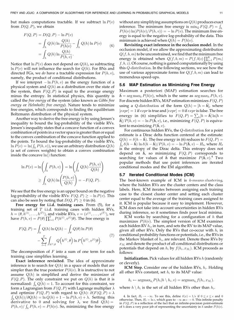
but makes computations tractable. If we subtract lnP ðvÞfrom DðQ;P Þ, we obtain

F ðQ;P Þ ¼ DðQ;P Þ � lnP ðvÞ

¼Zh

QðhÞ ln QðhÞP ðhjvÞ �

Zh

QðhÞ lnP ðvÞ

¼Zh

QðhÞ ln QðhÞP ðh; vÞ :

ð6Þ

Notice that lnP ðvÞ does not depend on QðhÞ, so subtractinglnP ðvÞ will not influence the search for QðhÞ. For BNs anddirected FGs, we do have a tractable expression for P ðh; vÞ,namely, the product of conditional distributions.

If we interpret � lnP ðh; vÞ as the energy function of aphysical system and QðhÞ as a distribution over the state ofthe system, then F ðQ;P Þ is equal to the average energyminus the entropy. In statistical physics, this quantity iscalled the free energy of the system (also known as Gibbs freeenergy or Helmholtz free energy). Nature tends to minimizefree energies, which corresponds to finding the equilibriumBoltzmann distribution of the physical system.

Another way to derive the free energy is by using Jensen’sinequality to bound the log-probability of the visible RVs.Jensen’s inequality states that a concave function of a convexcombinationofpoints inavector space isgreater thanor equalto the convex combination of the concave function applied tothe points. To bound the log-probability of the visible RVs,lnP ðvÞ ¼ lnð

Rh P ðh; vÞÞ, we use an arbitrary distributionQðhÞ

(a set of convex weights) to obtain a convex combinationinside the concave lnðÞ function:

lnP ðvÞ ¼ ln

Zh

P ðh; vÞ!¼ ln

Zh

QðhÞP ðh; vÞQðhÞ

!

�Zh

QðhÞ ln P ðh; vÞQðhÞ

!¼ �F ðQ;P Þ:

We see that the free energy is an upper bound on the negativelog-probability of the visible RVs: F ðQ;P Þ � � lnP ðvÞ. Thiscan also be seen by noting thatDðQ;P Þ � 0 in (6).

Free energy for i.i.d. training cases. From (5), for atraining set of T i.i.d. training cases with hidden RVs,h ¼ ð�; hð1Þ; . . . ; hðT ÞÞ, and visible RVs, v ¼ ðvð1Þ; . . . ; vðT ÞÞ, wehave P ðh; vÞ ¼ P ð�Þ

QTt¼1 P ðhðtÞ; vðtÞj�Þ. The free energy is

F ðQ;P Þ ¼Zh

QðhÞ lnQðhÞ �Z�

Qð�Þ lnP ð�Þ

�XTt¼1

ZhðtÞ;�

Q hðtÞ; ��

lnP hðtÞ; vðtÞj��

:

ð7Þ

The decomposition of F into a sum of one term for eachtraining case simplifies learning.

Exact inference revisited. The idea of approximateinference is to search for QðhÞ in a space of models that aresimpler than the true posterior P ðhjvÞ. It is instructive to notassume QðhÞ is simplified and derive the minimizer ofF ðQ;P Þ. The only constraint we put on QðhÞ is that it isnormalized:

Rh QðhÞ ¼ 1. To account for this constraint, we

form a Lagrangian from F ðQ;P Þwith Lagrange multiplier �and optimize F ðQ;P Þ with regard to QðhÞ: @ðF ðQ;P Þ þ �Rh QðhÞÞ=@QðhÞ ¼ lnQðhÞ þ 1� lnP ðh; vÞ þ �. Setting thisderivative to 0 and solving for �, we find QðhÞ ¼P ðh; vÞ=

Rh P ðh; vÞ ¼ P ðhjvÞ. So, minimizing the free energy

without any simplifyingassumptionsonQðhÞproduces exactinference. The minimum free energy is minQ F ðQ;P Þ ¼

Rh

P ðhjvÞ lnðP ðhjvÞ=P ðh; vÞÞ ¼ � lnP ðvÞ. The minimum free en-ergy is equal to the negative log-probability of the data. Thisminimum is achieved whenQðhÞ ¼ P ðhjvÞ.

Revisiting exact inference in the occlusion model. In theocclusion model, if we allow the approximating distributionQðf; b;mÞ to beunconstrained,we find that theminimumfreeenergy is obtained when Qðf; b;mÞ ¼ P ðf; bjzÞ

QKi¼1 P ðmij

f; b; zÞ. Of course, nothing is gained computationally byusingthisQ-distribution. In the following sections, we see how theuse of various approximate forms for Qðf; b;mÞ can lead totremendous speed-ups.

5.6 MAP Estimation as Minimizing Free Energy

Maximum a posteriori (MAP) estimation searches for

hh ¼ argmaxh P ðhjvÞ, which is the same as argmaxh P ðh; vÞ.For discrete hiddenRVs,MAP estimationminimizesF ðQ;P Þusing a Q-distribution of the form QðhÞ ¼ ½h ¼ hh�, where

½expr� ¼ 1 if expr is true and ½expr� ¼ 0 if expr is false. The free

energy in (6) simplifies to F ðQ;P Þ ¼P

h½h ¼ hh� ln½h ¼hh�=P ðh; vÞ ¼ � lnP ðhh; vÞ, i.e., minimizing F ðQ;P Þ is equiva-lent to maximizing P ðhh; vÞ.

For continuous hidden RVs, the Q-distribution for a pointestimate is a Dirac delta function centered at the estimate:QðhÞ ¼ �ðh� hhÞ. The free energy in (6) reduces to F ðQ;P Þ ¼Rh �ðh� hhÞ ln �ðh� hhÞ=P ðh; vÞ ¼ � lnP ðhh; vÞ �H�, where H�

is the entropy of the Dirac delta. This entropy does notdepend on hh, so minimizing F ðQ;P Þ corresponds tosearching for values of hh that maximize P ðhh; vÞ.4 Twopopular methods that use point inferences are iteratedconditional modes and the EM algorithm.

5.7 Iterated Conditional Modes (ICM)

The best-known example of ICM is k-means clustering,where the hidden RVs are the cluster centers and the classlabels. Here, ICM iterates between assigning each trainingcase to the closest cluster center and setting each clustercenter equal to the average of the training cases assigned toit. ICM is popular because it easy to implement. However,ICM does not take into account uncertainties in hidden RVsduring inference, so it sometimes finds poor local minima.

ICM works by searching for a configuration of h thatmaximizes P ðhjvÞ. The simplest version of ICM examineseach hidden RV hi, in turn, and sets the RV to its MAP value,given all other RVs. Only the RVs that co-occur with hi inconditional probability functions or potentials, i.e., theRVs inthe Markov blanket of hi, are relevant. Denote these RVs byxMi

and denote the product of all conditional distributions orpotentials that depend on hi by fðhi; xMi

Þ. ICM proceeds asfollows:

Initialization. Pick values for all hidden RVs h (randomlyor cleverly).

ICM Step. Consider one of the hidden RVs, hi. Holdingall other RVs constant, set hi to its MAP value:

hi argmaxhiP ðhijh n hi; vÞ ¼ argmaxhifðhi; xMiÞ:

where h n hi is the set of all hidden RVs other than hi.


4. In fact, H� ! �1. To see this, define �ðxÞ ¼ 1=� if 0 � x � � and 0otherwise. Then, H� ¼ ln �, which goes to �1 as �! 0. This infinite penaltyin F ðQ;P Þ is a reflection of the fact that an infinite-precision point-estimateof h does a very poor job of representing the uncertainty in h under P ðhjvÞ.

Repeat for a fixed number of iterations or untilconvergence.

If hi is discrete, this procedure is straightforward. If hi iscontinuous and exact optimization of hi is not possible, itscurrent value can be used as the initial point for a searchalgorithm, such as a Newton method or a gradient-basedmethod.

The free energy for ICM is the free energy describedabove, for general point inferences.

ICM in the occlusion model. Even when the modelparameters in the occlusion model are known, the compu-tational cost of exact inference can be rather high. When thenumber of clusters J is large, examining all J2 configura-tions of the foreground class and the background class iscomputationally burdensome. For ICM in the occlusionmodel, the Q-distribution for the entire training set is

Q ¼ Y

k

�ð�k � ��kÞ! Y

k;i

�ð�ki � ��kiÞ! Y

k;i

�ð ki � kiÞ!

Yk;i

�ð�ki � ��kiÞ! Y

t

�bðtÞ ¼ bbðtÞ

�! Y

t

�f ðtÞ ¼ ff ðtÞ

�! Yt

Yi

�mðtÞi ¼ mm

ðtÞi

�!:

Substituting this Q-distribution and the P -distribution in (4)into the expression for the free energy in (7), we obtain thefollowing (assuming a uniform parameter prior):

F ¼�Xt

�ln ��ffðtÞ þ ln ��bbðtÞ

��Xt

Xi

mmðtÞi ln ��ffðtÞi

þ 1� mmðtÞi� �

ln 1� ��ff ðtÞi� �!

þXt

Xi

mmðtÞi

zðtÞi � ��ffðtÞi

� �2=2 ffðtÞi þ ln 2� ff ðtÞi

� �=2

!

þXt

Xi

1� mmðtÞi� �

zðtÞi � ��bbðtÞi

� �2=2 bbðtÞi

þ ln 2� bbðtÞi

� �=2

!�H:

H is the entropy of the �-functions and is constant duringoptimization. F measures the mismatch between the inputimage and the image obtained by combining the foregroundand background using the mask.

To minimize the free energy with regard to all RVs andparameters,we can iteratively solve for eachRVor parameterkeeping the other RVs and parameters fixed. These updatescan be applied in any order, but since the model parametersdepend on values of all hidden RVs, we first optimize for allhidden RVs and then optimize for model parameters.Furthermore, since, for every observation, the class RVsdepend on all pixels, when updating the hidden RVs, we firstvisit the mask values for all pixels and then the class RVs.

After all parameters and RVs are set to randomvalues, theupdatesareappliedrecursively, asdescribed inFig.5.Tokeepnotation simple, the “ ” symbol is droppedand in theupdatesfor the variables mi, b, and f , the training case index ðtÞ isdropped.

5.8 Block ICM and Conjugate Gradients

One problem with the simple version of ICM describedabove is its severe greediness. Suppose fðhi; xMi

Þ has almostthe same value for two different values of hi. ICM will pickone value for hi, discarding the fact that the other value ofhi is almost as good. This problem can be partly avoided byoptimizing subsets of h, instead of single elements of h. Ateach step of this block ICM method, a tractable subgraph ofthe graphical model is selected and all RVs in the subgraphare updated to maximize P ðh; vÞ. Often, this can be doneefficiently using the max-product algorithm [23]. Anexample of this method is training HMMs using the Viterbialgorithm to select the most probable state sequence. Forcontinuous hidden RVs, an alternative to block ICM is touse a joint optimizer, such as a conjugate gradients.

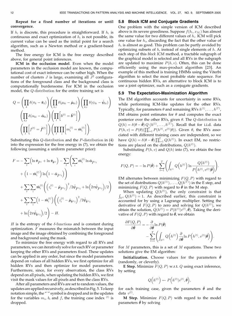
5.9 The Expectation-Maximization Algorithm

The EM algorithm accounts for uncertainty in some RVs,

while performing ICM-like updates for the other RVs.

Typically, for parameters � and remaining RVs hð1Þ; . . . ; hðT Þ,

EM obtains point estimates for � and computes the exact

posterior over the other RVs, given �. The Q-distribution is

QðhÞ ¼ �ð�� ÞQ ðhð1Þ; . . . ; hðT ÞÞ. Recall that for i.i.d. data

P ðh; vÞ ¼ P ð�ÞðQT

t¼1 P ðhðtÞ; vðtÞj�ÞÞ. Given �, the RVs asso-

ciated with different training cases are independent, so we

have QðhÞ ¼ �ð�� ÞQT

t¼1QðhðtÞÞ. In exact EM, no restric-

tions are placed on the distributions, QðhðtÞÞ.Substituting P ðh; vÞ and QðhÞ into (7), we obtain the free

energy:

F ðQ;P Þ ¼ � lnP ð��Þ þXTt¼1

ZhðtÞQ hðtÞ� �

lnQ hðtÞ� �

P hðtÞ; vðtÞj��

!:

EM alternates between minimizing F ðQ;P Þ with regard tothe set of distributions Qðhð1ÞÞ; . . . ; QðhðT ÞÞ in the E step, andminimizing F ðQ;P Þ with regard to �� in the M step.

When updating QðhðtÞÞ, the only constraint is thatRhðtÞ QðhðtÞÞ ¼ 1. As described earlier, this constraint isaccounted for by using a Lagrange multiplier. Setting thederivative of F ðQ;P Þ to zero and solving for QðhðtÞÞ, weobtain the solution, QðhðtÞÞ ¼ P ðhðtÞjvðtÞ; ��Þ. Taking the deri-vative of F ðQ;P Þwith regard to ��, we obtain

@F ðQ;P Þ@��

¼� @

@��lnP ð��Þ

�XTt¼1

ZhðtÞQ hðtÞ� � @

@��lnP hðtÞ; vðtÞj��

� �!:

For M parameters, this is a set of M equations. These twosolutions give the EM algorithm:

Initialization. Choose values for the parameters ��(randomly, or cleverly).

E Step. Minimize F ðQ;P Þ w.r.t. Q using exact inference,by setting

Q hðtÞ� �

P hðtÞjvðtÞ; ��

;

for each training case, given the parameters �� and thedata vðtÞ.

M Step. Minimize F ðQ;P Þ with regard to the modelparameters �� by solving


� @

@��lnP ð��Þ �

XTt¼1

ZhðtÞQ hðtÞ� � @

@��lnP hðtÞ; vðtÞj��

� �!¼ 0: ð8Þ

This is the derivative of the expected log-probability of the

complete data. For M parameters, this is a system of

M equations. Often, the prior on the parameters is assumed

to be uniform, P ð��Þ ¼ const, in which case, the first term in

the above expression vanishes.Repeat for a fixed number of iterations or until

convergence.

In Section 5.5, we showed that, when QðhÞ ¼ P ðhjvÞ,F ðQ;P Þ ¼ � lnP ðvÞ. So, theEMalgorithmalternatesbetween


Fig. 5a. Inference and learning algorithms for the occlusion model. Iverson’s notation is used, where ½expr� ¼ 1 if expr is true, and ½expr� ¼ 0 if expr is

false. The constant c is used to normalize distributions.

obtaininga tight lowerboundon lnP ðvÞand thenmaximizing

this bound with regard to the model parameters. This means

thatwith each iteration the log-probability of thedata, lnP ðvÞ,must increase or stay the same.

EM in the occlusion model. As with ICM, we approx-imate the distribution over the parameters using Qð�Þ ¼�ð�� Þ. As described above, in the E step, we setQðb; f;mÞ P ðb; f;mjzÞ for each training case, where, asdescribed in Section 5.4, P ðb; f;mjzÞ is represented in theform P ðb; f jzÞ

Qi P ðmijb; f; zÞ. This distribution is used in

the M step to minimize the free energy with regard to themodel parameters, � ¼ f�k; �k; k; �kgKk¼1. The resultingupdates are given in Fig. 5, where we have dropped thetraining case index in the E step for brevity and the constant cis computed to normalize the appropriate distribution.Starting with random parameters, the E and M steps areiterated until convergence or for a fixed number ofiterations.

5.10 Generalized EM

The above derivation of the EM algorithm makes obviousseveral generalizations, all of which attempt to decreaseF ðQ;P Þ [31]. If F ðQ;P Þ is a complex function of theparameters �, it may not be possible to exactly solve for the� that minimizes F ðQ;P Þ in the M step. Instead, � can bemodified so as to decrease F ðQ;P Þ, e.g., by taking a stepdownhill in the gradient of F ðQ;P Þ. Or, if � contains manyparameters, it may be that F ðQ;P Þ can be optimized withregard to one parameter while holding the others constant.Althoughdoing this does not solve the systemof equations, itdoes decrease F ðQ;P Þ.

Another generalization of EM arises when the posterior

distributionover thehiddenRVsis toocomplextoperformthe

exact update QðhðtÞÞ P ðhðtÞjvðtÞ; ��Þ that minimizes F ðQ;P Þin the E step. Instead, the distribution QðhðtÞÞ from the

previous E step can be modified to decrease F ðQ;P Þ. In fact,

ICM is a special case of EM where, in the E step, F ðQ;P Þ isdecreased by finding the value of hh

ðtÞthat minimizes F ðQ;P Þ

subject toQðhðtÞÞ ¼ �ðhðtÞ� hhðtÞÞ.

5.11 Gibbs Sampling and Monte Carlo Methods

Gibbs sampling is similar to ICM, but to circumvent localminima, Gibbs sampling stochastically selects the value ofhi at each step instead of picking the MAP value of hi:

Initialization. Pick values for all hidden RVs h (ran-domly or cleverly).

Gibbs Sampling Step. Consider one of the hidden RVs,hi. Holding all other RVs constant, sample hi:

hi � P ðhijh n hi; vÞ ¼ fðhi; xMiÞ=�X

hi

fðhi; xMiÞ�;

where xMiare the RVs in the Markov blanket of hi and

fðhi; xMiÞ is the product of all conditional distributions or

potentials that depend on hi.Repeat for a fixed number of iterations or until

convergence.

Algorithmically, this is a minor modification of ICM, but,in many applications, it is able to escape poor local minima(cf., [14], [18]). Also, the stochastically chosen values of hi canbe monitored to estimate the uncertainty in hi under theposterior.

If n counts the number of sampling steps, then as n!1thenth configurationof thehiddenRVs is guaranteed tobeanunbiased sample from the exact posterior P ðhjvÞ. In fact,although a single Gibbs sampler is not guaranteed to


Fig. 5b. (continued).

minimize the free energy, an infinite ensemble of Gibbssamplers does minimize free energy, regardless of the initialdistribution of the ensemble. Let QnðhÞ be the distributionover h given by the ensemble of samplers at step n. Supposewe obtain a new ensemble by sampling hi in each sampler.Then, Qnþ1ðhÞ ¼ Qnðh n hiÞP ðhijh n hi; vÞ. Substituting Qn

and Qnþ1 into (6), we find that Fnþ1 � Fn.Generally, inaMonteCarlomethod, thedistributionoverh

is represented by a set of configurations h1; . . . ; hS . Then, theexpected value of any function of the hidden RVs, fðhÞ, isapproximated by E½fðhÞ�� 1

S

PSs¼1 fðhsÞ. For example, if h

contains binary (0/1) RVs and h1; . . . ; hS are drawn fromP ðhjvÞ, then, by selecting fðhÞ ¼ hi, the above equation givesan estimate of P ðhi ¼ 1jvÞ. There are many approaches tosampling, but the two general classes of samplers are exactsamplers and Markov chain Monte Carlo (MCMC) samplers(cf., [30]). Whereas exact samplers produce a configurationwith probability equal to the probability under the model,MCMC samplers produce a sequence of configurations suchthat, in the limit, the configuration is a sample fromthemodel.If amodelP ðh; vÞ isdescribedbyaBN, thenanexact sampleofh and v can be obtained by successively sampling each RVgiven its parents, starting with parentless RVs and finishingwith childless RVs. Gibbs sampling is an example of anMCMC technique.

MCMC techniques and Gibbs sampling in particular areguaranteed to produce samples from the probability modelonly after the memory of the initial configuration hasvanished and the sampler has reached equilibrium. For thisreason, the sampler is often allowed to “burn in” beforesamples are used to compute Monte Carlo estimates. Thiscorresponds to discarding the samples obtained early on.

Gibbs sampling for EM in the occlusion model. Here,we describe a learning algorithm that uses ICM-updates forthe model parameters, but uses stochastic updates for theRVs. This technique can be viewed as a generalized EMalgorithm, where the E-Step is approximated by a Gibbssampler. Replacing the MAP RV updates in ICM withsampling, we obtain the algorithm in Fig. 5. The notationsampleb indicates the expression on the right should benormalized with regard to b and then b should be sampled.

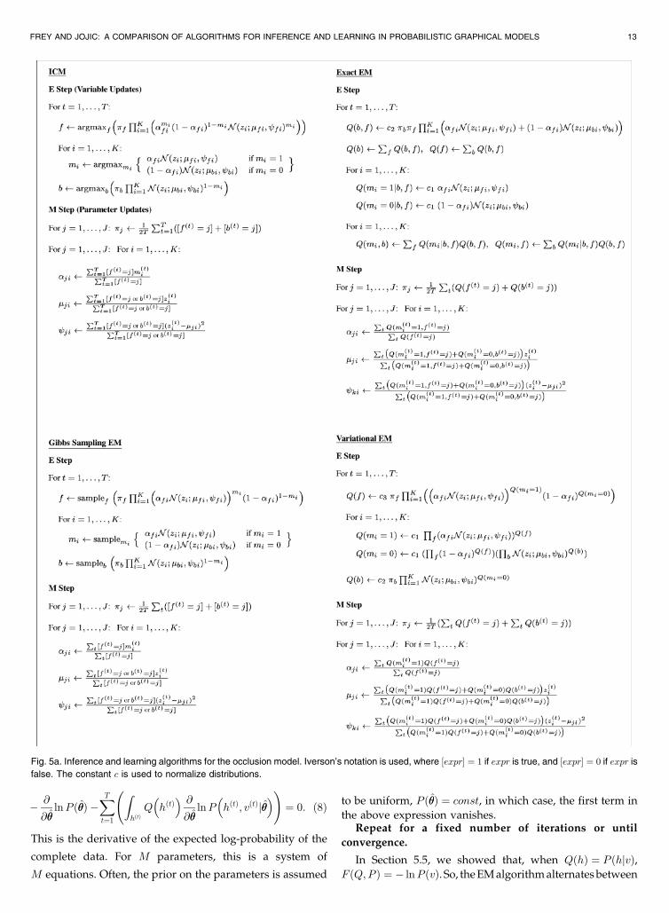
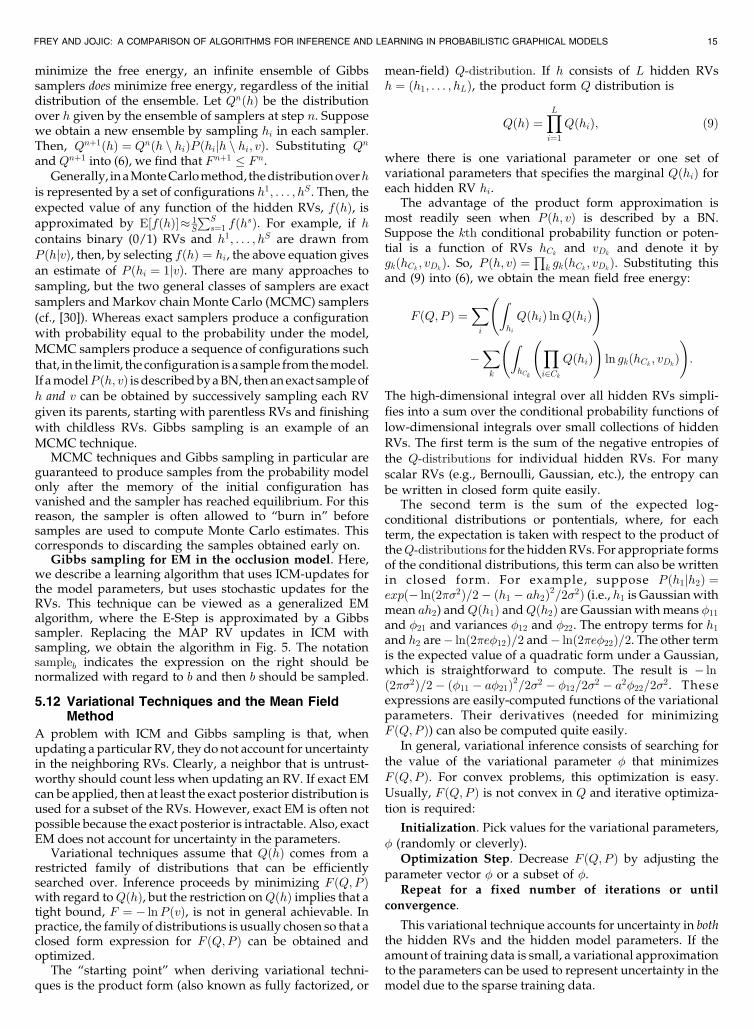
5.12 Variational Techniques and the Mean FieldMethod

A problem with ICM and Gibbs sampling is that, whenupdating a particular RV, they do not account for uncertaintyin the neighboring RVs. Clearly, a neighbor that is untrust-worthy should count less when updating an RV. If exact EMcan be applied, then at least the exact posterior distribution isused for a subset of the RVs. However, exact EM is often notpossible because the exact posterior is intractable. Also, exactEM does not account for uncertainty in the parameters.

Variational techniques assume that QðhÞ comes from arestricted family of distributions that can be efficientlysearched over. Inference proceeds by minimizing F ðQ;P Þwith regard toQðhÞ, but the restriction onQðhÞ implies that atight bound, F ¼ � lnP ðvÞ, is not in general achievable. Inpractice, the family of distributions is usually chosen so that aclosed form expression for F ðQ;P Þ can be obtained andoptimized.

The “starting point” when deriving variational techni-ques is the product form (also known as fully factorized, or

mean-field) Q-distribution. If h consists of L hidden RVsh ¼ ðh1; . . . ; hLÞ, the product form Q distribution is

QðhÞ ¼YLi¼1

QðhiÞ; ð9Þ

where there is one variational parameter or one set ofvariational parameters that specifies the marginal QðhiÞ foreach hidden RV hi.

The advantage of the product form approximation ismost readily seen when P ðh; vÞ is described by a BN.Suppose the kth conditional probability function or poten-tial is a function of RVs hCk and vDk

and denote it bygkðhCk ; vDk

Þ. So, P ðh; vÞ ¼Q

k gkðhCk ; vDkÞ. Substituting this

and (9) into (6), we obtain the mean field free energy:

F ðQ;P Þ ¼Xi

Zhi

QðhiÞ lnQðhiÞ!

�Xk

ZhCk

Yi2Ck

QðhiÞ!ln gk hCk ; vDkð Þ

!:

The high-dimensional integral over all hidden RVs simpli-fies into a sum over the conditional probability functions oflow-dimensional integrals over small collections of hiddenRVs. The first term is the sum of the negative entropies ofthe Q-distributions for individual hidden RVs. For manyscalar RVs (e.g., Bernoulli, Gaussian, etc.), the entropy canbe written in closed form quite easily.

The second term is the sum of the expected log-conditional distributions or pontentials, where, for eachterm, the expectation is taken with respect to the product oftheQ-distributions for the hiddenRVs. For appropriate formsof the conditional distributions, this term can also be writtenin closed form. For example, suppose P ðh1jh2Þ ¼expð� lnð2�2Þ=2� ðh1 � ah2Þ2=22Þ (i.e., h1 is Gaussianwithmean ah2) andQðh1Þ andQðh2Þ are Gaussian with means 11and 21 and variances 12 and 22. The entropy terms for h1and h2 are� lnð2�e12Þ=2 and� lnð2�e22Þ=2. The other termis the expected value of a quadratic form under a Gaussian,which is straightforward to compute. The result is � lnð2�2Þ=2� ð11 � a21Þ2=22 � 12=22 � a222=22. Theseexpressions are easily-computed functions of the variationalparameters. Their derivatives (needed for minimizingF ðQ;P Þ) can also be computed quite easily.

In general, variational inference consists of searching forthe value of the variational parameter that minimizesF ðQ;P Þ. For convex problems, this optimization is easy.Usually, F ðQ;P Þ is not convex in Q and iterative optimiza-tion is required:

Initialization. Pick values for the variational parameters, (randomly or cleverly).

Optimization Step. Decrease F ðQ;P Þ by adjusting theparameter vector or a subset of .

Repeat for a fixed number of iterations or until

convergence.

This variational technique accounts for uncertainty in boththe hidden RVs and the hidden model parameters. If theamount of training data is small, a variational approximationto the parameters can be used to represent uncertainty in themodel due to the sparse training data.


Often, variational techniques are used to approximate thedistribution over the hidden RVs in the E step of theEM algorithm, but point estimates are used for the modelparameters. In such variational EM algorithms, theQ-distribution is QðhÞ ¼ �ð�� Þ

QTt¼1QðhðtÞ;ðtÞÞ. Note that

there is one set of variational parameters for each trainingcase. In this case,wehave the followinggeneralizedEMsteps:

Initialization. Pick values for the variational parametersð1Þ; . . . ; ðT Þ and the model parameters �� (randomly orcleverly).

Generalized E Step. Starting from the variational para-meters from the previous iteration, modify ð1Þ; . . . ; ðT Þ so asto decrease F .

Generalized M Step. Starting from the model para-meters from the previous iteration, modify �� so as todecrease F .


Variational inference for EM in the occlusionmodel. The

fully factorizedQ-distributionover thehiddenRVsforasingle

data sample in the occlusion model is Qðm; f; bÞ ¼QðbÞQðfÞ

QKi¼1QðmiÞ. Substituting this Q-distribution into

the free energy for a single observed data sample in the

occlusion model, we obtain

F ¼Xb

QðbÞ lnQðbÞ�bþXf

QðfÞ lnQðfÞ�f

þXi

Xf

QðfÞ Qðmi ¼ 1Þ lnQðmi ¼ 1Þ

�fi

þQðmi ¼ 0Þ lnQðmi ¼ 0Þ1� �fi

!

þXi

Xf

QðfÞQðmi ¼ 1Þ ðzi � �fiÞ2

2 fiþ ln 2� fi

2

!

þXi

Qðmi ¼ 0Þ X

b

QðbÞ ðzi � �biÞ2

2 biþ ln 2� bi

2

!!:

The first two terms keepQðbÞ andQðfÞ close to their priors �band�f .The third termkeepsQðmiÞ close to themaskpriors�fifor foreground classes that have high posterior probability

QðfÞ. The last two terms favor mask values and foreground/

background classes that minimize the variance-normalized

squared differences between the predicted pixel values and

the observed pixel values.Setting the derivatives of F to zero, we obtain the updates

for the Q-distributions in the E step. Once the variationalparameters are computed for all observed images, the totalfree energyF ¼

Pt FðtÞ is optimizedwith regard to themodel

parameters to obtain the variational M step. The resultingupdates are given in Fig. 5. Each E step update can becomputed in OðKJÞ time, which is a K-fold speed-up overexact inference used for exact EM. This speed-up is obtainedbecause the variational method assumes that f and b areindependent in the posterior. Also, note that, if theQ-distribitions place all mass on one configuration, the E stepupdates reduce to the ICM updates The M step updates aresimilar to the updates for exact EM, except that the exactposterior distributions are replaced by their factorizedsurrogates.

The above updates can be iterated in a variety of ways.For example, each iteration may consist of repeatedlyupdating the variational distributions until convergenceand then updating the parameters. Or, each iteration mayconsist of updating each variational distribution once andthen updating the parameters. There are many possibilitiesand the update order that is best at avoiding local minimadepends on the problem.

5.13 Structured Variational Techniques

The product-form (mean-field) approximation does notaccount for dependencies between hidden RVs. For example,if the posterior has two distinct modes, the variationaltechnique for the product-form approximation will find onlyone mode. With a different initialization, the technique mayfind another mode, but the exact form of the dependence isnot revealed. In structured variational techniques [22], theQ-distribution is itself specified by a graphical model suchthat F ðQ;P Þ can still be optimized. Fig. 6a shows the originalBN for the occlusion model and Fig. 6b shows the BN for thefully factorized (mean field) Q-distribution described above.Recall that the exact posterior can be written P ðm; f; bjzÞ ¼Qðm; f; bÞ ¼ Qðf; bÞ

QKi¼1Qðmijf; bÞ. Fig. 6c shows the BN for

this Q-distribution. Generally, increasing the number ofdependencies in the Q-distribution leads to more exactinference algorithms, but also increases the computationaldemands of variational inference. In the occlusion model,whereas mean field inference takesKJ time, exact inferencetakes KJ2 time. However, additional dependencies cansometimes be accounted for at no extra computational cost.Asdescribed below, it turns out that theQ-distribution shownin Fig. 6d leads to an inference algorithm with the samecomplexity as the mean field method (KJ time), but canaccount for dependencies of themask RVs on the foregroundclass.

Structured variational inference for EM in the occlusionmodel. TheQ-distribution corresponding to the BN in Fig. 6disQðm; f; bÞ¼QðbÞQðfÞ

QKi¼1QðmijfÞ. Defining qfi ¼ Qðmi ¼

1jfÞ, we have Qðm; f; bÞ ¼ QðbÞQðfÞQK

i¼1 qmi

fi ð1� qfiÞ1�mi .

Substituting this Q-distribution into the free energy for theocclusion model, we obtain


Fig. 6. Starting with the BN of the original occlusion model (a) variationaltechniques ranging from the fully factorized approximation to exactinference can be derived. (b) The BN for the factorized (mean field)Q-distribution. z is observed, so it is not included in the graphical modelfor the Q-distribution. (c) The BN for a Q-distribution that can representthe exact posterior. (d) The BN for a Q-distribution that can representthe dependence of the mask RVs on the foreground class. Accountingfor more dependencies improves the bound on the data likelihood, butthe choice of which dependencies are retained has a large impact on theimprovement in the bound.

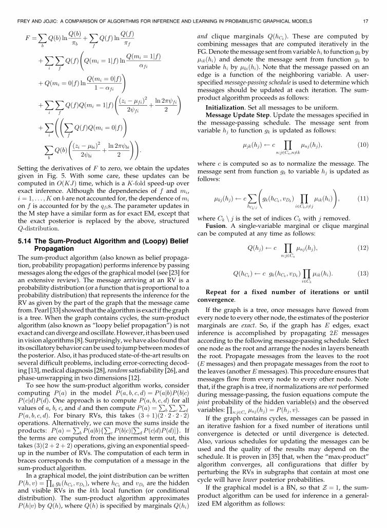
F ¼Xb

QðbÞ lnQðbÞ�bþXf

QðfÞ lnQðfÞ�f

þXi

Xf

QðfÞ Qðmi ¼ 1jfÞ lnQðmi ¼ 1jfÞ

�fi

þQðmi ¼ 0jfÞ lnQðmi ¼ 0jfÞ1� �fi

!

þXi

Xf

QðfÞQðmi ¼ 1jfÞ ðzi � �fiÞ2

2 fiþ ln 2� fi

2

!

þXi

Xf

QðfÞQðmi ¼ 0jfÞ!

Xb

QðbÞ ðzi � �biÞ2

2 biþ ln 2� bi

2

!!:

Setting the derivatives of F to zero, we obtain the updatesgiven in Fig. 5. With some care, these updates can becomputed in OðKJÞ time, which is a K-fold speed-up overexact inference. Although the dependencies of f and mi,i ¼ 1; . . . ; K on b are not accounted for, the dependence ofmi

on f is accounted for by the qfis. The parameter updates inthe M step have a similar form as for exact EM, except thatthe exact posterior is replaced by the above, structuredQ-distribution.

5.14 The Sum-Product Algorithm and (Loopy) BeliefPropagation

The sum-product algorithm (also known as belief propaga-tion, probability propagation) performs inference by passingmessages along the edges of the graphical model (see [23] foran extensive review). The message arriving at an RV is aprobability distribution (or a function that is proportional to aprobability distribution) that represents the inference for theRV as given by the part of the graph that the message camefrom.Pearl [33] showed that the algorithmis exact if thegraphis a tree. When the graph contains cycles, the sum-productalgorithm (also known as “loopy belief propagation”) is notexact andcandivergeandoscillate.However, it hasbeenusedinvision algorithms [8]. Surprisingly,wehave also found thatits oscillatory behavior canbeused to jumpbetweenmodes ofthe posterior. Also, it has produced state-of-the-art results onseveral difficult problems, including error-correcting decod-ing [13],medical diagnosis [28], random satisfiability [26], andphase-unwrapping in two dimensions [12].

To see how the sum-product algorithm works, considercomputing P ðaÞ in the model P ða; b; c; dÞ ¼ P ðajbÞP ðbjcÞP ðcjdÞP ðdÞ. One approach is to compute P ða; b; c; dÞ for allvalues of a, b, c, and d and then compute P ðaÞ ¼

Pb

Pc

Pd

P ða; b; c; dÞ. For binary RVs, this takes ð3þ 1Þð2 � 2 � 2 � 2Þoperations. Alternatively, we can move the sums inside theproducts: P ðaÞ ¼

Pb P ðajbÞf

Pc P ðbjcÞ½

Pd P ðcjdÞP ðdÞ�g. If

the terms are computed from the innermost term out, thistakes ð3Þð2þ 2þ 2Þ operations, giving an exponential speed-up in the number of RVs. The computation of each term inbraces corresponds to the computation of a message in thesum-product algorithm.

In a graphical model, the joint distribution can be writtenP ðh; vÞ ¼

Qk gkðhCk ; vDk

Þ, where hCk and vDkare the hidden

and visible RVs in the kth local function (or conditionaldistribution). The sum-product algorithm approximatesP ðhjvÞ by QðhÞ, where QðhÞ is specified by marginals QðhiÞ

and clique marginals QðhCkÞ. These are computed bycombining messages that are computed iteratively in theFG.Denote themessage sent fromvariablehi to function gk by�ikðhiÞ and denote the message sent from function gk tovariable hi by �kiðhiÞ. Note that the message passed on anedge is a function of the neighboring variable. A user-specifiedmessage-passing schedule is used to determine whichmessages should be updated at each iteration. The sum-product algorithm proceeds as follows:

Initialization. Set all messages to be uniform.Message Update Step. Update the messages specified in

the message-passing schedule. The message sent fromvariable hj to function gk is updated as follows:

�jkðhjÞ cY

n:j2Cn;n 6¼k�njðhjÞ; ð10Þ

where c is computed so as to normalize the message. Themessage sent from function gk to variable hj is updated asfollows:

�kjðhjÞ cXhCknj

gkðhCk ; vDk

ÞY

i2Ck;i 6¼j�ikðhiÞ

!; ð11Þ

where Ck n j is the set of indices Ck with j removed.Fusion. A single-variable marginal or clique marginal

can be computed at any time as follows:

QðhjÞ cY

n:j2Cn�njðhjÞ; ð12Þ

QðhCkÞ c gkðhCk ; vDkÞYi2Ck

�ikðhiÞ: ð13Þ


If the graph is a tree, once messages have flowed fromevery node to every other node, the estimates of the posteriormarginals are exact. So, if the graph has E edges, exactinference is accomplished by propagating 2E messagesaccording to the following message-passing schedule. Selectone node as the root and arrange the nodes in layers beneaththe root. Propagate messages from the leaves to the root(E messages) and then propagate messages from the root tothe leaves (anotherEmessages). This procedure ensures thatmessages flow from every node to every other node. Notethat, if the graph is a tree, if normalizations are not performedduring message-passing, the fusion equations compute thejoint probability of the hidden variable(s) and the observedvariables:

Qn:j2Cn �njðhjÞ ¼ P ðhj; vÞ.

If the graph contains cycles, messages can be passed inan iterative fashion for a fixed number of iterations untilconvergence is detected or until divergence is detected.Also, various schedules for updating the messages can beused and the quality of the results may depend on theschedule. It is proven in [35] that, when the “max-product”algorithm converges, all configurations that differ byperturbing the RVs in subgraphs that contain at most onecycle will have lower posterior probabilities.

If the graphical model is a BN, so that Z ¼ 1, the sum-product algorithm can be used for inference in a general-ized EM algorithm as follows:


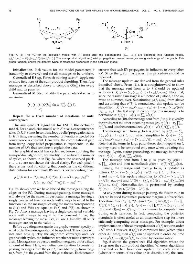
Initialization. Pick values for the model parameters �(randomly or cleverly) and set all messages to be uniform.

Generalized E Step. For each training case vðtÞ, apply oneor more iterations of the sum-product algorithm. Then, fusemessages as described above to compute QðhðtÞCkÞ for everychild and its parents.

Generalized M Step. Modify the parameters � so as tomaximize X

t

Xk

XhðtÞCk

QðhðtÞCkÞ ln gkðhðtÞCk; vðtÞDk; �Þ:


The sum-product algorithm for EM in the occlusionmodel. For an occlusionmodel withK pixels, exact inferencetakesOðKJ2Þ time. In contrast, loopybeliefpropagation takesOðKJÞ time, assuming the number of iterations needed forconvergence is constant. Generally, the computational gainfrom using loopy belief propagation is exponential in thenumber of RVs that combine to explain the data.

The graphical model has cycles, so, before applying thesum-product algorithm, we modify it to reduce the numberof cycles, as shown in in Fig. 7a, where the observed pixelsz1; . . . ; zK are not shown for visual clarity. For each pixel i,there is one local function gi that combines the conditionaldistributions for each mask RV and its corresponding pixel:

giðf; b;miÞ ¼ P ðzijmi; f; bÞP ðmijfÞ ¼ N ðzi;�fi; fiÞmi

Nðzi;�bi; biÞ1�mi�mi

fi ð1� �fiÞ1�mi :

Fig. 7b shows how we have labeled the messages along theedges of the FG. During message passing, some messageswill always be the same. In particular, a message leaving asingly connected function node will always be equal to thefunction. So, the messages leaving the nodes correspondingto P ðfÞ and P ðbÞ are equal to P ðfÞ and P ðbÞ, as shown inFig. 7b. Also, a message leaving a singly-connected variablenode will always be equal to the constant 1. So, themessages leaving the mask RVs, mi, are 1. Initially, all othermessages are set to the value 1.

Before updatingmessages in the graph,wemust specify inwhat order themessages should be updated. This choice willinfluence how quickly the algorithm converges and, forgraphswith cycles, can influence whether or not it convergesat all.Messages can be passed until convergence or for a fixedamount of time. Here, we define one iteration to consist ofpassingmessages from the gs to b, from b to the gs, from the gsto f , from f to the gs, and from the gs to thems. Each iteration

ensures that each RV propagates its influence to every otherRV. Since the graph has cycles, this procedure should berepeated.

The message updates are derived from the general rulesdescribed above. From (11), it is straightforward to showthat the message sent from gi to f should be updatedas follows: �fi ðfÞ

Pb

Pmi�biðbÞ � 1 � giðf; b;miÞ. Note that,

since the resulting message is a function of f alone, b andmi

must be summed over. Substituting giðf; b;miÞ from aboveand assuming that �biðbÞ is normalized, this update can besimplified: �fi ðfÞ �fiNðzi;�fi; fiÞ þ ð1� �fiÞ

Pb �

biðbÞN

ðzi;�bi; biÞ. The last step in computing this message is tonormalize it: �fi ðfÞ �fi ðfÞ=ð

Pf �

fi ðfÞÞ.

According to (10), themessage sent from f to gi is given bythe product of the other incomingmessages, �fi ðfÞ �f

Qj6¼i

�fi ðfÞ, and it is then normalized: �fi ðfÞ �fi ðfÞ=ðP

f �fi ðfÞ.

The message sent from gi to b is given by �biðbÞ P

fPmi�fi ðfÞ � 1 � giðf; b;miÞ, which simplifies to �biðbÞ

�Pf

�fi ðfÞ�fiNðzi;�fi; fiÞ�þ�P

f �fi ðfÞð1� �fiÞ

�Nðzi;�bi; biÞ.

Note that the terms in large parentheses don’t depend on b,

so they need to be computed only once when updating this

message. Again, before proceeding, the message is normal-

ized: �biðbÞ �biðbÞ=ðP

b �biðbÞÞ.

The message sent from b to gi is given by �biðbÞ �bQ

j 6¼i �biðbÞ and then normalized: �biðbÞ �biðbÞ=ð

Pb �

biðbÞ.

Finally, the message sent from gi to mi is updated as

follows: �mi ðmiÞ P

f

Pb �

fi ðfÞ � �biðbÞ � giðf; b;miÞ. Formi ¼

1 and mi ¼ 0, this update simplifies to �mi ð1Þ P

f �fi ðfÞ

�fiNðzi;�fi; fiÞ and �mi ð0Þ �P

f �fi ðfÞð1� �fiÞ

��Pb �

biðbÞ

N ðzi;�bi; biÞ�. Normalization is performed by setting

�mi ðmiÞ �mi ðmiÞ=ð�mi ð0Þ þ �mi ð1ÞÞ.At any point during message-passing, the fusion rule in

(12) can be used to estimate posterior marginals of variables.

TheestimatesofP ðf jzÞ,P ðbjzÞandP ðmijzÞareQðfÞ ��fQ

i

�fi ðfÞ�=�P

f �fQ

i �fi ðfÞ

�, QðbÞ

��bQ

i �biðbÞ�=�P

b �bQ

i �bi

ðbÞ�, and QðmiÞ �mi ðmiÞ. It is common to compute these

during each iteration. In fact, computing the posterior

marginals is often useful as an intermediate step for more

efficiently computing other messages. For example, direct

implementation of the above updates for �fi ðfÞ requires orderJK2 time. However, if QðfÞ is computed first (which takes

order JK time), then �fi ðfÞ can be updated in order JK time

using �fi ðfÞ QðfÞ=�fi ðfÞ, followed by normalization.Fig. 5 shows the generalized EM algorithm where the

E step uses the sum-product algorithm. Whereas algorithmspresented earlier have one update for each variable(whether in terms of its value or its distribution), the sum-


Fig. 7. (a) The FG for the occlusion model with K pixels after the observations (z1; . . . ; zK ) are absorbed into function nodes,

giðf; b;miÞ ¼ P ðzijmi; f; bÞP ðmijfÞ. (b) The sum-product algorithm (belief propagation) passes messages along each edge of the graph. This

graph fragment shows the different types of messages propagated in the occlusion model.

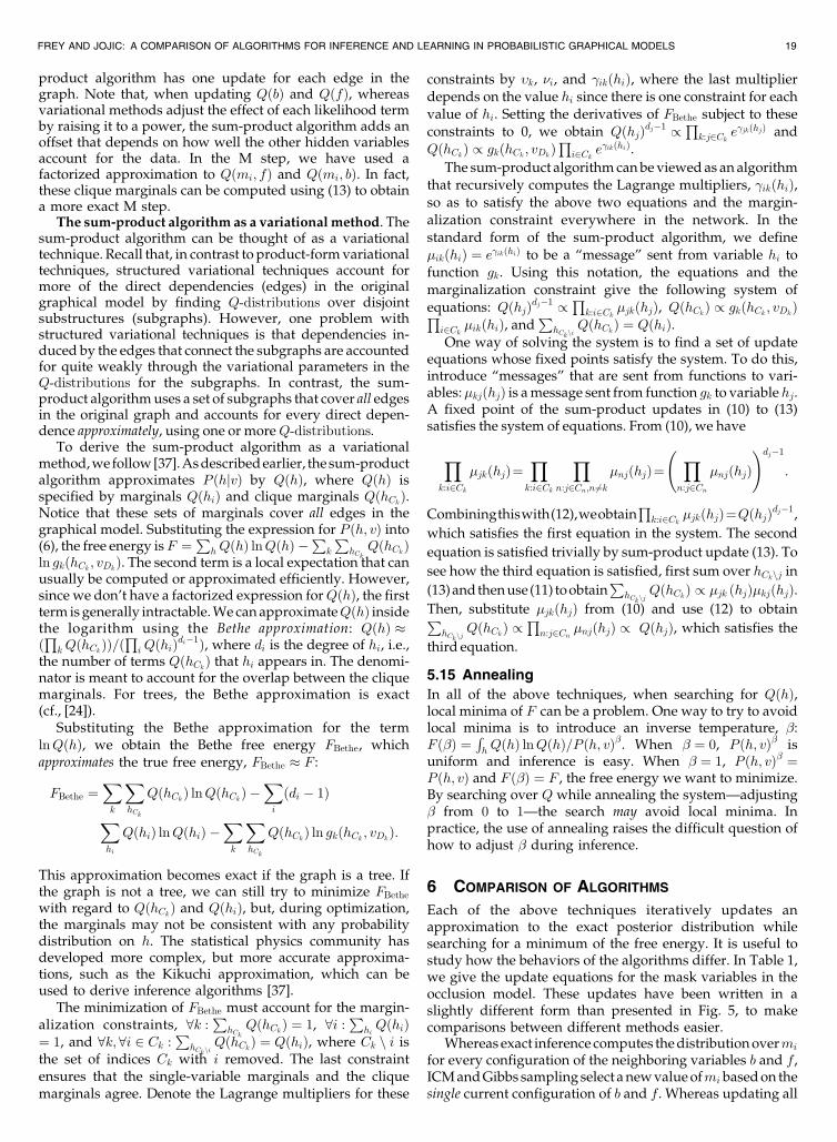
product algorithm has one update for each edge in thegraph. Note that, when updating QðbÞ and QðfÞ, whereasvariational methods adjust the effect of each likelihood termby raising it to a power, the sum-product algorithm adds anoffset that depends on how well the other hidden variablesaccount for the data. In the M step, we have used afactorized approximation to Qðmi; fÞ and Qðmi; bÞ. In fact,these clique marginals can be computed using (13) to obtaina more exact M step.

The sum-product algorithm as a variationalmethod. Thesum-product algorithm can be thought of as a variationaltechnique. Recall that, in contrast to product-formvariationaltechniques, structured variational techniques account formore of the direct dependencies (edges) in the originalgraphical model by finding Q-distributions over disjointsubstructures (subgraphs). However, one problem withstructured variational techniques is that dependencies in-duced by the edges that connect the subgraphs are accountedfor quite weakly through the variational parameters in theQ-distributions for the subgraphs. In contrast, the sum-product algorithmuses a set of subgraphs that cover all edgesin the original graph and accounts for every direct depen-dence approximately, using one or moreQ-distributions.

To derive the sum-product algorithm as a variationalmethod,wefollow[37].Asdescribedearlier, thesum-productalgorithm approximates P ðhjvÞ by QðhÞ, where QðhÞ isspecified by marginals QðhiÞ and clique marginals QðhCkÞ.Notice that these sets of marginals cover all edges in thegraphical model. Substituting the expression for P ðh; vÞ into(6), the free energy isF ¼

Ph QðhÞ lnQðhÞ �

Pk

PhCk

QðhCkÞln gkðhCk ; vDk

Þ. The second term is a local expectation that canusually be computed or approximated efficiently. However,since we don’t have a factorized expression forQðhÞ, the firstterm is generally intractable.WecanapproximateQðhÞ insidethe logarithm using the Bethe approximation: QðhÞ �ðQ

k QðhCkÞÞ=ðQ

i QðhiÞdi�1Þ, where di is the degree of hi, i.e.,

the number of terms QðhCkÞ that hi appears in. The denomi-nator is meant to account for the overlap between the cliquemarginals. For trees, the Bethe approximation is exact(cf., [24]).

Substituting the Bethe approximation for the termlnQðhÞ, we obtain the Bethe free energy FBethe, whichapproximates the true free energy, FBethe � F :

FBethe ¼Xk

XhCk

QðhCkÞ lnQðhCkÞ �Xi

ðdi � 1Þ

Xhi

QðhiÞ lnQðhiÞ �Xk

XhCk

QðhCkÞ ln gkðhCk ; vDkÞ:

This approximation becomes exact if the graph is a tree. Ifthe graph is not a tree, we can still try to minimize FBethe

with regard to QðhCkÞ and QðhiÞ, but, during optimization,the marginals may not be consistent with any probabilitydistribution on h. The statistical physics community hasdeveloped more complex, but more accurate approxima-tions, such as the Kikuchi approximation, which can beused to derive inference algorithms [37].

The minimization of FBethe must account for the margin-alization constraints, 8k :

PhCk

QðhCkÞ ¼ 1, 8i :P

hiQðhiÞ

¼ 1, and 8k; 8i 2 Ck :P

hCkniQðhCkÞ ¼ QðhiÞ, where Ck n i is

the set of indices Ck with i removed. The last constraintensures that the single-variable marginals and the cliquemarginals agree. Denote the Lagrange multipliers for these

constraints by �k, i, and �ikðhiÞ, where the last multiplierdepends on the value hi since there is one constraint for eachvalue of hi. Setting the derivatives of FBethe subject to theseconstraints to 0, we obtain QðhjÞdj�1 /

Qk:j2Ck e

�jkðhjÞ andQðhCkÞ / gkðhCk ; vDk

ÞQ

i2Ck e�ikðhiÞ.

The sum-product algorithmcanbeviewedas an algorithmthat recursively computes the Lagrange multipliers, �ikðhiÞ,so as to satisfy the above two equations and the margin-alization constraint everywhere in the network. In thestandard form of the sum-product algorithm, we define�ikðhiÞ ¼ e�ikðhiÞ to be a “message” sent from variable hi tofunction gk. Using this notation, the equations and themarginalization constraint give the following system ofequations: QðhjÞdj�1 /

Qk:i2Ck �jkðhjÞ, QðhCkÞ / gkðhCk ; vDk

ÞQi2Ck �ikðhiÞ, and

PhCkni

QðhCkÞ ¼ QðhiÞ.One way of solving the system is to find a set of update

equations whose fixed points satisfy the system. To do this,introduce “messages” that are sent from functions to vari-ables:�kjðhjÞ is amessage sent from function gk to variable hj.A fixed point of the sum-product updates in (10) to (13)satisfies the system of equations. From (10), we have

Yk:i2Ck

�jkðhjÞ¼Yk:i2Ck

Yn:j2Cn;n 6¼k

�njðhjÞ¼ Yn:j2Cn

�njðhjÞ!dj�1

:

Combiningthiswith(12),weobtainQ

k:i2Ck �jkðhjÞ¼QðhjÞdj�1,

which satisfies the first equation in the system. The second

equation is satisfied trivially by sum-product update (13). To

see how the third equation is satisfied, first sum over hCknj in

(13)andthenuse (11) toobtainP

hCknjQðhCkÞ / �jk ðhjÞ�kjðhjÞ.

Then, substitute �jkðhjÞ from (10) and use (12) to obtainPhCknj

QðhCkÞ /Q

n:j2Cn �njðhjÞ / QðhjÞ, which satisfies the

third equation.

5.15 Annealing

In all of the above techniques, when searching for QðhÞ,local minima of F can be a problem. One way to try to avoidlocal minima is to introduce an inverse temperature, �:F ð�Þ ¼

Rh QðhÞ lnQðhÞ=P ðh; vÞ

�. When � ¼ 0, P ðh; vÞ� isuniform and inference is easy. When � ¼ 1, P ðh; vÞ� ¼P ðh; vÞ and F ð�Þ ¼ F , the free energy we want to minimize.By searching over Q while annealing the system—adjusting� from 0 to 1—the search may avoid local minima. Inpractice, the use of annealing raises the difficult question ofhow to adjust � during inference.

6 COMPARISON OF ALGORITHMS

Each of the above techniques iteratively updates anapproximation to the exact posterior distribution whilesearching for a minimum of the free energy. It is useful tostudy how the behaviors of the algorithms differ. In Table 1,we give the update equations for the mask variables in theocclusion model. These updates have been written in aslightly different form than presented in Fig. 5, to makecomparisons between different methods easier.

Whereas exact inference computes thedistributionovermi

for every configuration of the neighboring variables b and f ,ICMandGibbs sampling select anewvalueofmi basedon thesingle current configuration of b and f . Whereas updating all


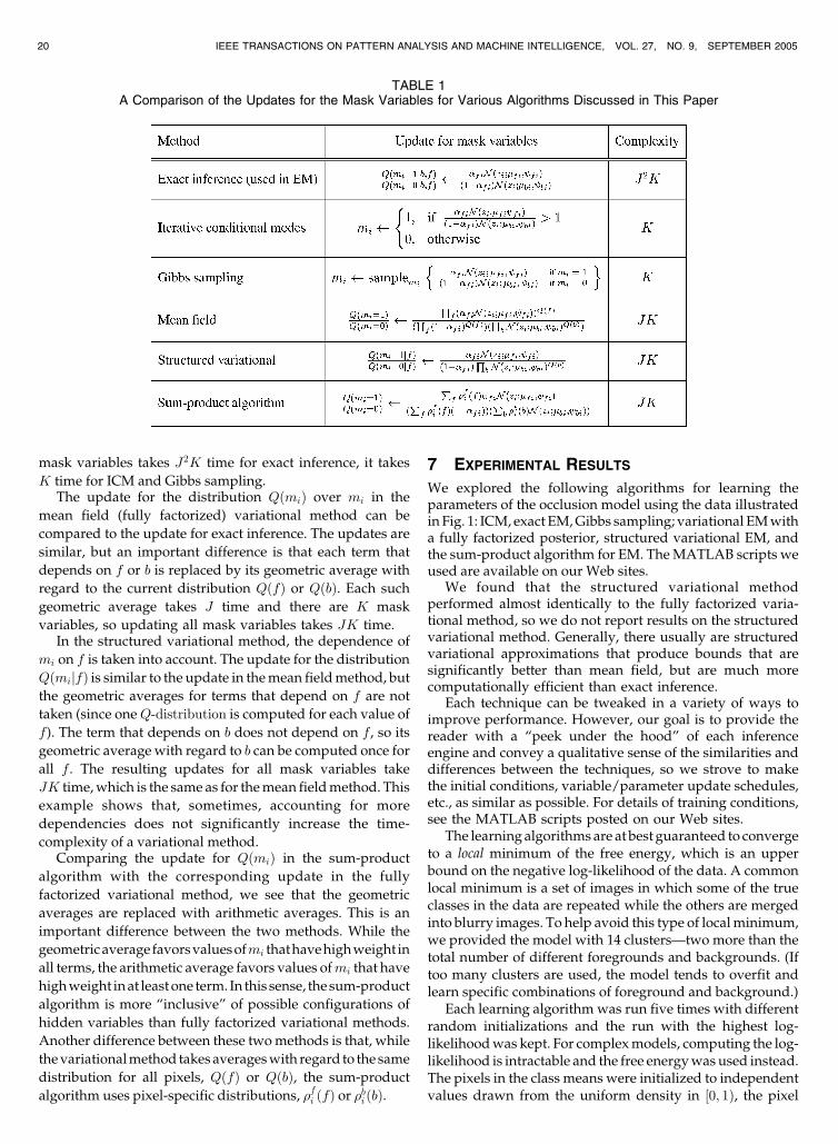
mask variables takes J2K time for exact inference, it takes

K time for ICM and Gibbs sampling.The update for the distribution QðmiÞ over mi in the

mean field (fully factorized) variational method can be

compared to the update for exact inference. The updates are

similar, but an important difference is that each term that

depends on f or b is replaced by its geometric average with

regard to the current distribution QðfÞ or QðbÞ. Each such

geometric average takes J time and there are K mask

variables, so updating all mask variables takes JK time.In the structured variational method, the dependence of

mi on f is taken into account. The update for the distribution

QðmijfÞ is similar to the update in themean fieldmethod, but

the geometric averages for terms that depend on f are not

taken (since oneQ-distribution is computed for each value of

f). The term that depends on b does not depend on f , so its

geometric averagewith regard to b can be computed once for

all f . The resulting updates for all mask variables take

JK time,which is the same as for themean fieldmethod. This

example shows that, sometimes, accounting for more

dependencies does not significantly increase the time-

complexity of a variational method.Comparing the update for QðmiÞ in the sum-product

algorithm with the corresponding update in the fully

factorized variational method, we see that the geometric

averages are replaced with arithmetic averages. This is an

important difference between the two methods. While the

geometricaveragefavorsvaluesofmi thathavehighweight in

all terms, the arithmetic average favors values ofmi that have

highweight inat leastone term. In this sense, thesum-product

algorithm is more “inclusive” of possible configurations of

hidden variables than fully factorized variational methods.

Another difference between these twomethods is that, while

thevariationalmethod takesaverageswith regard to the same

distribution for all pixels, QðfÞ or QðbÞ, the sum-product

algorithm uses pixel-specific distributions, �fi ðfÞ or �biðbÞ.

7 EXPERIMENTAL RESULTS

We explored the following algorithms for learning theparameters of the occlusion model using the data illustratedinFig. 1: ICM, exact EM,Gibbs sampling; variational EMwitha fully factorized posterior, structured variational EM, andthe sum-product algorithm for EM. TheMATLAB scripts weused are available on our Web sites.

We found that the structured variational methodperformed almost identically to the fully factorized varia-tional method, so we do not report results on the structuredvariational method. Generally, there usually are structuredvariational approximations that produce bounds that aresignificantly better than mean field, but are much morecomputationally efficient than exact inference.

Each technique can be tweaked in a variety of ways toimprove performance. However, our goal is to provide thereader with a “peek under the hood” of each inferenceengine and convey a qualitative sense of the similarities anddifferences between the techniques, so we strove to makethe initial conditions, variable/parameter update schedules,etc., as similar as possible. For details of training conditions,see the MATLAB scripts posted on our Web sites.

The learningalgorithmsare at best guaranteed to convergeto a local minimum of the free energy, which is an upperbound on the negative log-likelihood of the data. A commonlocal minimum is a set of images in which some of the trueclasses in the data are repeated while the others are mergedinto blurry images. To help avoid this type of localminimum,we provided the model with 14 clusters—two more than thetotal number of different foregrounds and backgrounds. (Iftoo many clusters are used, the model tends to overfit andlearn specific combinations of foreground and background.)

Each learning algorithm was run five times with differentrandom initializations and the run with the highest log-likelihoodwas kept. For complexmodels, computing the log-likelihood is intractable and the free energywasused instead.The pixels in the class means were initialized to independentvalues drawn from the uniform density in ½0; 1Þ, the pixel


TABLE 1A Comparison of the Updates for the Mask Variables for Various Algorithms Discussed in This Paper

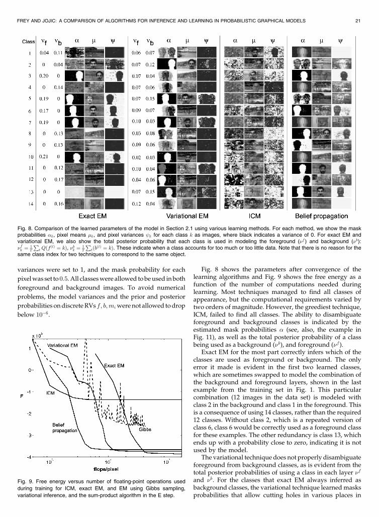
variances were set to 1, and the mask probability for each

pixelwas set to 0:5.All classeswere allowed tobeused inboth

foreground and background images. To avoid numerical

problems, the model variances and the prior and posterior

probabilities ondiscreteRVs f; b;miwerenot allowed todrop

below 10�6.

Fig. 8 shows the parameters after convergence of thelearning algorithms and Fig. 9 shows the free energy as afunction of the number of computations needed duringlearning. Most techniques managed to find all classes ofappearance, but the computational requirements varied bytwo orders of magnitude. However, the greediest technique,ICM, failed to find all classes. The ability to disambiguateforeground and background classes is indicated by theestimated mask probabilities � (see, also, the example inFig. 11), as well as the total posterior probability of a classbeing used as a background ( b), and foreground ( f ).

Exact EM for the most part correctly infers which of theclasses are used as foreground or background. The onlyerror it made is evident in the first two learned classes,which are sometimes swapped to model the combination ofthe background and foreground layers, shown in the lastexample from the training set in Fig. 1. This particularcombination (12 images in the data set) is modeled withclass 2 in the background and class 1 in the foreground. Thisis a consequence of using 14 classes, rather than the required12 classes. Without class 2, which is a repeated version ofclass 6, class 6 would be correctly used as a foreground classfor these examples. The other redundancy is class 13, whichends up with a probability close to zero, indicating it is notused by the model.

The variational technique does not properly disambiguateforeground from background classes, as is evident from thetotal posterior probabilities of using a class in each layer f

and b. For the classes that exact EM always inferred asbackground classes, the variational technique learned masksprobabilities that allow cutting holes in various places in


Fig. 8. Comparison of the learned parameters of the model in Section 2.1 using various learning methods. For each method, we show the maskprobabilities �k, pixel means �k, and pixel variances k for each class k as images, where black indicates a variance of 0. For exact EM andvariational EM, we also show the total posterior probability that each class is used in modeling the foreground ( f ) and background ( b): fk ¼ 1

T

Pt Qðf ðtÞ ¼ kÞ, bk ¼ 1

T

PtðbðtÞ ¼ kÞ. These indicate when a class accounts for too much or too little data. Note that there is no reason for the

same class index for two techniques to correspond to the same object.

Fig. 9. Free energy versus number of floating-point operations used

during training for ICM, exact EM, and EM using Gibbs sampling,

variational inference, and the sum-product algorithm in the E step.

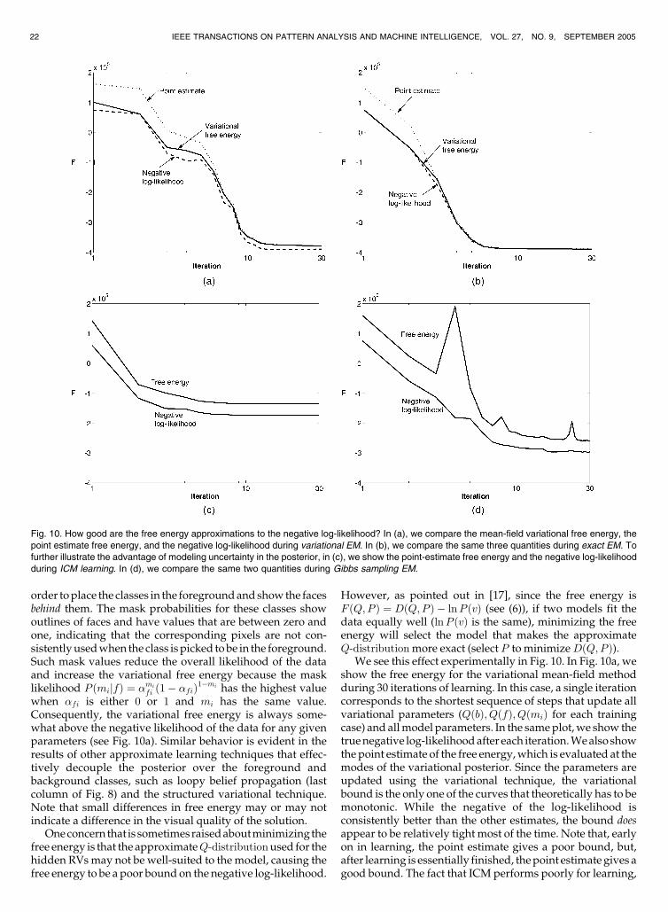
order toplace the classes in the foregroundandshowthe facesbehind them. The mask probabilities for these classes showoutlines of faces and have values that are between zero andone, indicating that the corresponding pixels are not con-sistentlyusedwhen the class ispicked tobe in the foreground.Such mask values reduce the overall likelihood of the dataand increase the variational free energy because the masklikelihood P ðmijfÞ ¼ �mi

fi ð1� �fiÞ1�mi has the highest value

when �fi is either 0 or 1 and mi has the same value.Consequently, the variational free energy is always some-what above the negative likelihood of the data for any givenparameters (see Fig. 10a). Similar behavior is evident in theresults of other approximate learning techniques that effec-tively decouple the posterior over the foreground andbackground classes, such as loopy belief propagation (lastcolumn of Fig. 8) and the structured variational technique.Note that small differences in free energy may or may notindicate a difference in the visual quality of the solution.

Oneconcernthat is sometimesraisedaboutminimizing thefree energy is that the approximateQ-distributionused for thehidden RVsmay not be well-suited to the model, causing thefree energy to be a poor boundon the negative log-likelihood.

However, as pointed out in [17], since the free energy isF ðQ;P Þ ¼ DðQ;P Þ � lnP ðvÞ (see (6)), if two models fit thedata equally well (lnP ðvÞ is the same), minimizing the freeenergy will select the model that makes the approximateQ-distributionmore exact (select P to minimizeDðQ;P Þ).

We see this effect experimentally in Fig. 10. In Fig. 10a, weshow the free energy for the variational mean-field methodduring 30 iterations of learning. In this case, a single iterationcorresponds to the shortest sequence of steps that update allvariational parameters (QðbÞ; QðfÞ; QðmiÞ for each trainingcase) and allmodel parameters. In the sameplot,we show thetruenegative log-likelihoodafter each iteration.Wealso showthe point estimate of the free energy,which is evaluated at themodes of the variational posterior. Since the parameters areupdated using the variational technique, the variationalbound is the only one of the curves that theoretically has to bemonotonic. While the negative of the log-likelihood isconsistently better than the other estimates, the bound doesappear to be relatively tight most of the time. Note that, earlyon in learning, the point estimate gives a poor bound, but,after learning is essentially finished, thepoint estimate gives agood bound. The fact that ICM performs poorly for learning,


Fig. 10. How good are the free energy approximations to the negative log-likelihood? In (a), we compare the mean-field variational free energy, the

point estimate free energy, and the negative log-likelihood during variational EM. In (b), we compare the same three quantities during exact EM. To

further illustrate the advantage of modeling uncertainty in the posterior, in (c), we show the point-estimate free energy and the negative log-likelihood

during ICM learning. In (d), we compare the same two quantities during Gibbs sampling EM.

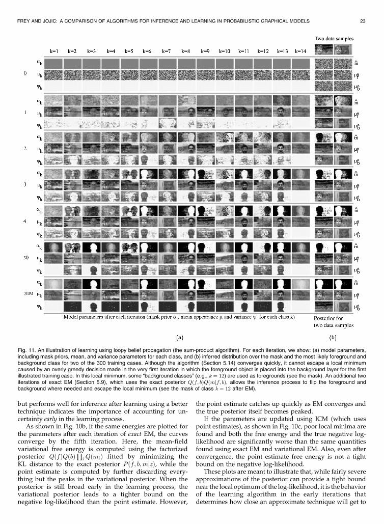
but performs well for inference after learning using a bettertechnique indicates the importance of accounting for un-certainty early in the learning process.

As shown in Fig. 10b, if the same energies are plotted forthe parameters after each iteration of exact EM, the curvesconverge by the fifth iteration. Here, the mean-fieldvariational free energy is computed using the factorizedposterior QðfÞQðbÞ

Qi QðmiÞ fitted by minimizing the

KL distance to the exact posterior P ðf; b;mjzÞ, while thepoint estimate is computed by further discarding every-thing but the peaks in the variational posterior. When theposterior is still broad early in the learning process, thevariational posterior leads to a tighter bound on thenegative log-likelihood than the point estimate. However,

the point estimate catches up quickly as EM converges andthe true posterior itself becomes peaked.

If the parameters are updated using ICM (which usespoint estimates), as shown in Fig. 10c, poor local minima arefound and both the free energy and the true negative log-likelihood are significantly worse than the same quantitiesfound using exact EM and variational EM. Also, even afterconvergence, the point estimate free energy is not a tightbound on the negative log-likelihood.

These plots are meant to illustrate that, while fairly severeapproximations of the posterior can provide a tight boundnear the local optimumof the log-likelihood, it is the behaviorof the learning algorithm in the early iterations thatdetermines how close an approximate technique will get to


Fig. 11. An illustration of learning using loopy belief propagation (the sum-product algorithm). For each iteration, we show: (a) model parameters,including mask priors, mean, and variance parameters for each class, and (b) inferred distribution over the mask and the most likely foreground andbackground class for two of the 300 training cases. Although the algorithm (Section 5.14) converges quickly, it cannot escape a local minimumcaused by an overly greedy decision made in the very first iteration in which the foreground object is placed into the background layer for the firstillustrated training case. In this local minimum, some “background classes” (e.g., k ¼ 12) are used as foregrounds (see the mask). An additional twoiterations of exact EM (Section 5.9), which uses the exact posterior Qðf; bÞQðmjf; bÞ, allows the inference process to flip the foreground andbackground where needed and escape the local minimum (see the mask of class k ¼ 12 after EM).

a local optimum of the the true log-likelihood. In the earlyiterations, to give the model a chance to get to a good localoptimum, the model parameters are typically initialized tomodel broad distributions, allowing the learning techniquesto more broadly explore the space of possibilities throughrelatively flat posteriors (e.g., in our case, we initialize thevariances to be equal to one, corresponding to a standarddeviation of 100percent of thedynamic range of the image). Ifthe approximate posterior makes greedy decisions early inthe learning process, it is often difficult to correct the errors inlater iterations. ICM, while very fast, is the most greedy of allthe techniques. Even if variances are initialized to largevalues, ICMmakes poor, greedy decisions for the configura-tion of the hidden RVs early on in learning and does notrecover from these mistakes.

Importantly, even computationally simple ways of ac-counting for uncertainty can improve performance signifi-cantly, incomparisonwith ICM. InFig.10d,weshowthepointestimate free energyand thenegative log-likelihoodwhen theICM technique is modified to take some uncertainty intoaccount by performing a Gibbs sampling step for each RVinsteadofpicking themostprobablevalue.5Thismethoddoesnot increase the computational cost per iteration compared toICM, but it obtains much better values of both energies.Sampling sometimesmakes the free energyworse during thelearning, but allows the algorithm to account for uncertaintyearly on, when the true posterior distributions for RVs arebroad. While this single-step Gibbs sampling techniqueobtains better energies than ICM, it does not achieve thelower energies obtained by exact EM and variational EM.

The effect of approximate probabilistic inference on thevisual quality of the parameters is illustrated in Fig. 11,wherewe show how the model parameters change during severaliterations of EMwhere the E step is performedusing the sum-product algorithm. On the far right of the figure, we illustratethe inference over hidden RVs (foreground class f , back-ground class b, and the maskm) for two training cases. Afterthe first iteration, while finding good guesses for the classesthat took part in the formation process, the foreground andbackground are incorrectly inverted in the posterior for thefirst training case and this situation persists even afterconvergence. Interestingly, by applying an additional twoiterations of exact EM after 30 iterations of sum-product EM,the model leaves the local minimum. This is evident not onlyin the first trainingcase, but also in the restof the trainingdata,as evidenced by the erasure of holes in the estimated maskprobabilities for the background classes. The same improve-ment can be observed for the variational technique. In fact,adding a small number of exact EM iterations to improve theresults of variational learning can be seen as part of the sameframework of optimizing the variational free energy, exceptthat not only the parameters of the variational posterior, butalso its form can be varied to increase the bound at each step.

When the nature of the local minima to which a learningtechnique is susceptible iswell understood, it is oftenpossibleto changeeither themodel or the formof theapproximation tothe posterior to avoid these minima without too much extracomputation. In the occlusion model, the problem is thebackground-foreground inversion, which can be avoided bysimply testing the inversion hypothesis and switching theinferred background and foreground classes to check if this

lowers the free energy, rather than exploring all possiblecombinations of classes in the exact posterior.An elegantwayof doing this within the variational framework is to add anadditional “switch”RV to themodel,which, in the generativeprocess, can switch the two classes. Then, the mean fieldposterior would have a component that models the un-certaintyabout foreground-background inversion.While thiswould render the variational learning two times slower, itwould still be much faster than the exact EM.

8 FUTURE DIRECTIONS

In our view, themost interesting and potentially high-impactareas of current research include introducing effectiverepresentations andmodels of data; inventing new inferenceand learning algorithms that can efficiently infer combinator-ial explanations of data; developing real-time, or near-real-time, modular software systems that enable researchers anddevelopers to evaluate the effectiveness of combinations ofinference and learning algorithms for solving real-worldtasks; advancing techniques for combining information frommultiple sources, e.g., camera images, spectral features,microphones, text, tactile information, etc.; developinginference algorithms for active tasks, that effectively accountfor uncertainties in the sensory inputs and the model of theenvironment whenmaking decisions about investigating theenvironment. In our view, a core requirement in all of thesedirections of research is that uncertainty should be properlyaccounted for, both in the representations of problems and inadapting to new data. Large-scale, hierarchical probabilitymodels and efficient inference and learning algorithms willplay a large role in the successful implementation of thesesystems.

REFERENCES

[1] E.H. Adelson and P. Anandan, “Ordinal Characteristics ofTransparency,” Proc. AAAI Workshop Qualitative Vision, 1990.

[2] O.E. Barndorff-Nielson, Information and Exponential Families.Chichester: Wiley, 1978.

[3] J. Besag, “ On the Statistical Analysis of Dirty Pictures,” J. RoyalStatistical Soc. B, vol. 48, pp. 259-302, 1986.

[4] R.G. Cowell, A.P. Dawid, S.L. Lauritzen, and D.J. Spiegelhalter,Probabilistic Networks and Expert Systems. New York: Springer,1999.

[5] R.G. Cowell, A.P. Dawid, and P. Sebastiani, “A Comparison ofSequential Learning Methods for Incomplete Data,” J. BayesianStatistics, vol. 5, pp. 581-588, 1996.

[6] A.P. Dempster, N.M. Laird, and D.B. Rubin, “Maximum Like-lihood from Incomplete Data via the EM Algorithm,” Proc. RoyalStatistical Soc., vol. 39, pp. 1-38, 1977.

[7] Hermann von Helmholtz, D. Cahan, ed. Los Angeles: Univ. of Calif.Press, 1993.

[8] W. Freeman and E. Pasztor, “Learning Low-Level Vision,” Proc.Int’l Conf. Computer Vision, pp. 1182-1189, 1999.

[9] B.J. Frey, “Extending Factor Graphs so as to Unify Directed andUndirected Graphical Models,” Proc. 19th Conf. Uncertainty inArtificial Intelligence, 2003.

[10] B.J. Frey and N. Jojic, “Transformed Component Analysis: JointEstimation of Spatial Transformations and Image Components,”Proc. IEEE Int’l Conf. Computer Vision, Sept. 1999.

[11] B.J. Frey and N. Jojic, “Transformation-Invariant Clustering Usingthe EM Algorithm,” IEEE Trans. Pattern Analysis and MachineIntelligence, vol. 25, no. 1, pp. 1-17, Jan. 2003.

[12] B.J. Frey, R. Koetter, and N. Petrovic, “Very Loopy BeliefPropagation for Unwrapping Phase Images,” Advances in NeuralInformation Processing Systems 14, T.G. Dietterich, S. Becker, andZ. Ghahramani, eds. MIT Press, 2002.


5. Note that, because this technique does not use an ensemble of samples,it is not guaranteed to minimize free energy at each step.

[13] B.J. Frey and D.J.C. MacKay, “A Revolution: Belief Propagation inGraphs with Cycles,” Advances in Neural Information ProcessingSystems 1997,M.I. Jordan, M.I. Kearns, and S.A. Solla, eds., vol. 10.pp. 479-485. MIT Press, 1998.

[14] S. Geman and D. Geman, “Stochastic Relaxation, Gibbs Distribu-tion and the Bayesian Restoration of Images,” IEEE Trans. PatternAnalysis and Machine Intelligence, vol. 6, pp. 721-741, 1984.

[15] Z. Ghahramani and M. Beal, “Propagation algorithms forVariational Bayesian Learning,” Advances in Neural InformationProcessing Systems 13, T. Leen, T. Dietterich, and V. Tresp, eds.MIT Press, 2001.

[16] D. Heckerman, “A Tutorial on Learning with Bayesian Net-works,” Learning in Graphical Models, M.I. Jordan, ed. Norwell,Mass.: Kluwer Academic, 1998.

[17] G.E. Hinton, P. Dayan, B.J. Frey, and R.M. Neal, “The Wake-SleepAlgorithm for Unsupervised Neural Networks,” Science, vol. 268,pp. 1158-1161, 1995.

[18] G.E. Hinton and T.J. Sejnowski, “Learning and Relearning inBoltzmann Machines,” Parallel Distributed Processing: Explorationsin the Microstructure of Cognition, D.E. Rumelhart and J.L. McClel-land, eds., vol. I, pp. 282-317, 1986.

[19] N. Jojic and B.J. Frey, “Learning Flexible Sprites in Video Layers,”Proc. IEEE Conf. Computer Vision and Pattern Recognition, 2001.

[20] N. Jojic, B.J. Frey, and A. Kannan, “Epitomic Analysis ofAppearance and Shape,” Proc. IEEE Int’l Conf. Computer Vision,Sept. 2003.

[21] N. Jojic, N. Petrovic, B.J. Frey, and T.S. Huang, “TransformedHidden Markov Models: Estimating Mixture Models of Imagesand Inferring Spatial Transformations in Video Sequences,” Proc.IEEE Conf. Computer Vision and Pattern Recognition, June 2000.

[22] M.I. Jordan, Z. Ghahramani, T.S. Jaakkola, and L.K. Saul, “AnIntroduction to Variational Methods for Graphical Models,”Learning in Graphical Models, M.I. Jordan, ed. Norwell, Mass.:Kluwer Academic, 1998.

[23] F.R. Kschischang, B.J. Frey, and H.-A. Loeliger, “Factor Graphsand the Sum-Product Algorithm,” IEEE Trans. Information Theory,special issue on codes on graphs and iterative algorithms, vol. 47,no. 2, pp. 498-519, Feb. 2001.

[24] S.L. Lauritzen, Graphical Models. New York: Oxford Univ. Press,1996.

[25] D.J.C. MacKay, “Bayesian Neural Networks and Density Net-works,” Nuclear Instruments and Methods in Physics Research,vol. 354, pp. 73-80, 1995.

[26] M. Mezard, G. Parisi, and R. Zecchina, “Analytic and AlgorithmicSolution of Random Satisfiability Problems,” Science, vol. 297,pp. 812-815, 2002.

[27] T.P. Minka, “Expectation Propagation for Approximate BayesianInference,” Proc. 17th Conf. Uncertainty in Artificial Intelligence, 2001.

[28] K.P. Murphy, Y. Weiss, and M.I. Jordan, “Loopy Belief Propaga-tion for Approximate Inference: An Empirical Study,” Proc. 15thConf. Uncertainty in Artificial Intelligence, 1999.

[29] R.M. Neal, “Bayesian Mixture Modeling by Monte Carlo Simula-tion,” Technical Report CRG-TR-91-2, Univ. of Toronto, 1991.

[30] R.M. Neal, “Probabilistic Inference Using Markov Chain MonteCarlo Methods,” technical report, Univ. of Toronto, 1993.

[31] R.M. Neal and G.E. Hinton, “A View of the EM Algorithm thatJustifies Incremental, Sparse, and Other Variants,” Learning inGraphical Models, M.I. Jordan, ed. pp. 355-368, Norwell, Mass.:Kluwer Academic, 1998.

[32] A.Y. Ng and M.I. Jordan, “A Comparison of Logistic Regressionand Naive Bayes,” Advances in Neural Information ProcessingSystems 14, T. G. Dietterich, S. Becker, and Z. Ghahramani, eds.,Cambridge, Mass.: MIT Press, 2002.

[33] J. Pearl, Probabilistic Reasoning in Intelligent Systems. San Mateo,Calif.: Morgan Kaufmann, 1988.

[34] M.J. Wainwright and M.I. Jordan, “Graphical Models, VariationalInference and Exponential Families,” Technical Report 649, Dept.of Statistics, Univ. of California, Berkeley, 2003.

[35] Y. Weiss and W. Freeman, “On the Optimaility of Solutions of theMax-Product Belief Propagation Algorithm in Arbitrary Graphs,”IEEE Trans. Information Theory, special issue on codes on graphsand iterative algorithms, vol. 47, no. 2, pp. 736-744, Feb. 2001.

[36] C.W. Williams and M.K. Titsias, “Learning about Multiple Objectsin Images: Factorial Learning without Factorial Search,” Advancesin Neural Information Processing Systems 15, S. Becker, S. Thrun, andK. Obermayer, eds., Cambridge, Mass.: MIT Press, 2003.

[37] J. Yedidia, W.T. Freeman, and Y. Weiss, “Understanding BeliefPropagation and Its Generalizations,” Proc. Int’l Joint Conf.Artificial Intelligence, 2001.

Brendan J. Frey’s university education includedengineering, physics, and computer science,culminating with a doctorate from GeoffreyHinton’s Neural Networks Research Group atthe University of Toronto. From 1997 to 1999, hewas a Beckman Fellow at the University ofIllinois at Urbana-Champaign, where he con-tinues to be an adjunct faculty member inelectrical and computer engineering. From1998 to 2001, he was a faculty member in

computer science at the University of Waterloo. Currently, he is the headof the Probabilistic and Statistical Inference Group in the Department ofElectrical and Computer Engineering at the University of Toronto andconsults for Microsoft Research, Redmond, Washington. He hasreceived several awards, given more than 40 invited talks, andpublished more than 100 papers on probabilistic inference and machinelearning for computer vision, computational biology, and informationprocessing. In the past, he cochaired the Workshop on ArtificialIntelligence and Statistics and the Canadian Workshop on InformationTheory and acted as co-editor-in-chief of a special issue of the IEEETransactions on Information Theory, titled Codes on Graphs andIterative Algorithms. He was also an associate editor of the IEEETransactions on Pattern Analysis and Machine Intelligence. He is asenior member of the IEEE.

Nebojsa Jojic received the PhD degree fromthe University of Illinois at Urbana-Champaign in2001, where he received a Microsoft Fellowshipin 1999 and a Robert T. Chien excellence inresearch award in 2000. He has been aresearcher at Microsoft Research in Redmond,Washington, since 2000. Dr. Jojic also spent asemester at the University of Illinois at Chicagoand consulted for the Hong Kong University ofScience and Technology. He has published

more than 40 papers in the areas of computer vision, machine learning,signal processing, computer graphics, and computational biology.

. For more information on this or any other computing topic,please visit our Digital Library at www.computer.org/publications/dlib.


A comparison of algorithms for inference and learning - Probabilistic

Documents