A comparison of a GCM response to historical anthropogenic land cover change and model sensitivity to uncertainty in present-day land cover representations

Johannes Feddema Æ Keith Oleson Æ Gordon Bonan

Linda Mearns Æ Warren Washington Æ Gerald Meehl

Douglas Nychka

A comparison of a GCM response to historical anthropogenic land coverchange and model sensitivity to uncertainty in present-day land coverrepresentations

Received: 10 August 2004 / Accepted: 5 May 2005 / Published online: 11 August 2005� Springer-Verlag 2005

Abstract This study assesses the sensitivity of the fullycoupled NCAR-DOE PCM to three different represen-tations of present-day land cover, based on IPCC SRESland cover information. We conclude that there is sig-nificant model sensitivity to current land cover charac-terization, with an observed average global temperaturerange of 0.21 K between the simulations. Much largercontrasts (up to 5 K) are found on the regional scale;however, these changes are largely offsetting on theglobal scale. These results show that significant biasescan be introduced when outside data sources are used toconduct anthropogenic land cover change experimentsin GCMs that have been calibrated to their own repre-sentation of present-day land cover. We conclude thathybrid systems that combine the natural vegetation fromthe native GCM datasets combined with human landcover information from other sources are best for sim-ulating such impacts. We also performed a prehumansimulation, which had a 0.39 K �higher average globaltemperature and, perhaps of greater importance, tem-perature changes regionally of about 2 K. In this study,the larger regional changes coincide with large-scaleagricultural areas. The initial cooling from energy bal-ance changes appear to create feedbacks that intensifymid-latitude circulation features and weaken the sum-mer monsoon circulation over Asia, leading to furthercooling. From these results, we conclude that land coverchange plays a significant role in anthropogenicallyforced climate change. Because these changes coincide

with regions of the highest human population this cli-mate impact could have a disproportionate impact onhuman systems. Therefore, it is important that landcover change be included in past and future climatechange simulations.

1 Introduction

Humans have altered the surface of the Earth signifi-cantly over the last few millennia and numerous studieshave demonstrated these effects and simulated theircauses (e.g., Betts 2001; Bonan 1999; Chase et al. 2000;Claussen et al. 2001; Costa and Foley 2000; Eastmanet al. 2001; Henderson-Sellers et al. 1993; Nobre et al.1991; Pielke and Avissar 1990; Pielke 2001; Pitman andZhao 2000; Tsvetsinskaya et al. 2001; Williams andBalling 1996). There is a growing awareness that theseprocesses cannot be ignored in future climate changesimulations (Hansen et al. 1998; Pielke et al. 2002;Mahoney et al. 2003; Marland et al. 2003; Bounouaet al. 2002). Yet, these effects have not been included inIPCC scenario simulations (IPCC 2001). There are sev-eral reasons why they have not. First, land surfacemodels in GCMs have only recently matured to thepoint where they can effectively simulate these changes(Avissar 1995; Pielke et al. 2002). Second, documentinghuman land cover change adequately for such studies isvery complex (Nakicenovic and Swart 2000). In addi-tion, we have little knowledge of the consequences ofusing different land surface characterizations in GCMsimulations (Oleson et al. 2004; Myhre and Myhre2003).

Uncertainties in GCM responses to land coverchange simulations fall into two major categories.First, uncertainty arises from differences in the modelsthemselves. For example, the Project for the Inter-comparison of Land surface Parameterization Schemes(PILPS) showed that given identical land cover char-acteristics, different land surface models gave disparate

J. Feddema (&)Department of Geography, University of Kansas,Lawrence, KS, 66045 USAE-mail: [email protected].: +1-785-8645534Fax: +1-303-4971695

K. Oleson Æ G. Bonan Æ L. Mearns Æ W. WashingtonG. Meehl Æ D. NychkaNational Center for Atmospheric Research,Boulder, CO, 80305 USA

Climate Dynamics (2005) 25: 581–609DOI 10.1007/s00382-005-0038-z

surface energy balance outcomes (Henderson-Sellerset al. 1993; Chen et al. 1997; Boone et al. 2004).Second, uncertainty arises from differences in the wayland cover is represented in different land cover clas-sification schemes (Oleson et al. 2004; Myhre andMyhre 2003). Land cover characterizations vary widelydepending on the modeling group and modelingschemes used (e.g., Cox et al. 1999; Bonan 1994; Peylinet al. 1997). Furthermore, model surface characteriza-tions are typically different from the land coverschemes used in the IPCC Special Report on Emis-sions Scenarios land cover change products(Nakicenovic and Swart 2000).

This study assesses the sensitivity of a fully coupledocean–atmosphere GCM to different present-day landcover representations, and will compare this uncertaintyto the simulated climate change caused by historicalanthropogenic land cover modification. As part of thisstudy, we will use readily available SRES land coverchange information to evaluate these issues (Nakiceno-vic and Swart 2000; Alcamo 1994; Alcamo et al. 1998).Simulations use the Department of Energy ParallelClimate Model (DOE-PCM; Washington et al. 2000).This model has been used to assess a number of IPCCclimate change scenarios, thereby providing a valuableframe of reference for this study. Specifically, we addressthe following questions:

1. What is the sensitivity of a fully coupled generalcirculation model to different present-day land coverrepresentations?

2. Given that models are calibrated with respect tospecific land cover representations, what is the bestmethod for including alternative land cover scenariosinto GCM simulations?

3. Has human land cover change had a significant im-pact on climate? Is this signal sufficiently large tosuggest the need for including land cover change aspart of IPCC based climate change scenarios?

4. Are global statistics adequate to detect climate signalsfrom land cover change? Is there a discernable spatialpattern associated with land cover induced climatechange?

2 Methods

We use the DOE-PCM (Washington et al. 2000). Thismodel has been used to study a number of natural andhuman induced climate forcings (Ammann et al. 2003;Meehl et al. 2003; Santer et al. 2003a, b). The resolutionof the atmosphere is T42, or roughly 2.8·2.8�, with 18levels in the vertical. Resolution in the ocean is roughly2/3 degree down to 1/2 degree in the equatorial tropics,with 32 levels. Sea ice is simulated using dynamic andthermodynamic formulations (Washington et al. 2000),and the NCAR Land Surface Model (NCAR LSM) isused as the land surface component (Bonan 1998). Noflux corrections are used in the model, and a relativelystable climate is simulated in terms of global-mean

temperature. For example, a preindustrial 1,000-yearlong control integration shows only a small coolingtrend of globally averaged surface air temperatures ofroughly 0.03 K per century.

To test the sensitivity of the DOE-PCM to land covervariations, we devised two sets of experiments. First, weevaluated the model response to three different ‘‘present-day’’ land cover representations: (1) the land coverscheme used in the NCAR LSM (labeled as LSMlchereafter); (2) the IMAGE 2.2 present-day land cover, asdocumented in the IPCC SRES documentation (Alcamo1994; Alcamo et al. 1998; Nakicenovic and Swart 2000;labeled as IMAlc hereafter); and (3) a hybrid land coverwhere the background vegetation was in accordancewith the original NCAR LSM land cover types and thehuman land cover types were derived from the IMAGE2.2 present-day land cover classifications (labeled HYBlchereafter). Second, to evaluate the potential historicalimpact of anthropogenic land cover change on climate,we compared simulations using the IMAGE 2.2 poten-tial vegetation, representing prehuman conditions (la-beled POTlc hereafter), and the commensurate present-day IMAGE 2.2 (IMAlc) land cover. We used the IM-AGE 2.2 based scenarios because the NCAR LSM landcover dataset has no equivalent potential vegetationdataset and because this will facilitate comparisons toother IMAGE 2.2 based land cover simulations, whichwill be discussed in future work. Land cover is fixed foreach simulation, and agriculture is represented as a mixof 85 percent crop vegetation and 15% bare ground.Phenological characteristics of the crop vegetation aretypical of those for a mid-latitude summer crop, withgreening starting in April, LAI reaching a maximum ofthree in late summer, and senescence ending by lateOctober (see Bonan 1996). In the Southern Hemisphere,the timing of phenology is offset by 6 months from theNorthern Hemisphere (Bonan 1996).

Each land cover experiment consisted of a DOE-PCM simulation run for 100 years with preindustrialatmospheric conditions (280 ppm CO2 concentrations).An existing preindustrial 1,000 year long-term controlintegration (no variation in forcing over time), with thestandard NCAR LSM land cover was used for theLSMlc climate. Simulations were started from this runin the model year 400. The simulations were allowed toreach equilibrium over the first 60 years, and the last40 years of the simulations were used for analysis pur-poses.

3 Development of the land cover datasets

The IPCC special report on emissions scenarios(Nakicenovic and Swart 2000) presents results from sixdifferent research groups who independently compiledand modeled data to characterize future emissions sce-narios. These simulations provided data on greenhousegas (GHG) concentrations and aerosols over time, butseveral of the groups also included information on land

582 Feddema et al.: A comparison of a GCM response to historical anthropogenic land cover change and model sensitivity

cover as part of their scenario simulations. We usedIPCC compatible land cover conditions as simulated bythe IMAGE 2.2 model (Alcamo 1994; Alcamo et al.1998). All data were obtained from the IMAGE 2.2CDROM released by the Netherlands EnvironmentalAssessment Agency (Rijksinstituut voor Volksgezond-heid en Milieu; RIVM 2002) and represent the condi-tions presented in the IPCC SRES report for theIMAGE 2.2 scenario simulations (Nakicenovic andSwart 2000).

The IMAGE 2.2 land cover changes are based on anumber of assumptions and databases. Base or controlexperiments are derived from datasets calibrated to 1970conditions (Alcamo 1994; Alcamo et al. 1998; RIVM2002). As part of the land cover scenarios a potentialvegetation dataset representing prehuman conditionswas created using the IMAGE 2.2 Terrestrial VegetationModel (Leemans and van den Born 1994; Alcamo et al.1998), which in turn uses a modified version of theBIOME model (Prentice et al. 1992).

Development of the land cover datasets required thatall land cover characterizations fit the biome type landcover classifications used in the NCAR LSM. Thismodel allows for the representation of 22 unique land

cover classifications originally derived from the Olsonet al. (1983) half-degree global vegetation database(Bonan 1996). The IMAGE 2.2 datasets use 18 landcover classes that differ from those used in the NCARLSM. The present-day IMAGE 2.2 derived land coverdataset was created by finding the dominant IMAGE 2.2land cover class in a T42 grid cell and converting this tothe equivalent NCAR LSM land cover class (Table 1;IMAlc, Fig. 1). To create the Hybrid dataset (HYBlc),the IMAGE 2.2 human land cover types were aggre-gated to the T42 grid size and then overlaid onto theNCAR LSM natural vegetation land cover types. TheIMAGE 2.2 potential vegetation (POTlc) was created byaggregating the IMAGE 2.2 potential vegetation typesto the T42 grid resolution and then converted to NCARLSM land cover classes (Table 1; Fig. 1).

Treatment for the Hybrid land cover dataset (HYBlc)was slightly different and combined the IMAGE 2.2SRES human land cover classification data (agricultureand degraded grassland classes) together with theNCAR LSM natural vegetation land cover classifica-tions. If the aggregated IMAGE 2.2 agricultural landcover class for a T42 grid cell was dominant, i.e., greaterthan 50% of the area, the cell was classified as agricul-

Fig. 1 Land cover representations used for the a LSMlc, b IMAlc, c HYBlc and d POTlc land cover experiments

Feddema et al.: A comparison of a GCM response to historical anthropogenic land cover change and model sensitivity 583

ture. If the IMAGE 2.2 degraded grassland was domi-nant, then the T42 grid cell was assigned the NCARLSM grassland land cover class. For those locationswhere a human land cover type was in the minority, andwhere the original NCAR LSM dataset had a humanland cover type, the new natural vegetation type was

determined by the dominant natural vegetation type ofthe surrounding grid cells and checked for reasonableaccuracy against the Ramankutty and Foley (1999) po-tential vegetation class. When required, the conversionwas based on the Ramankutty and Foley (1999) poten-tial vegetation class (Table 2).

Table 2 Conversion criteria totranslate Ramankutty andFoley (1999) potentialvegetation land cover classes toNCAR LSM land cover classes

R&F potential land cover class NCAR LSM land cover class

Tropical evergreen forest/woodland Tropical broadleaf evergreen tree (10)Tropical deciduous forest/woodland Tropical broadleaf evergreen tree (10)Temperate broadleaf evergreen forest/woodland Broadleaf deciduous tree (8)Temperate needleleaf evergreen forest/woodland Needleleaf evergreen tree (3)Temperate deciduous forest/woodland Broadleaf deciduous tree (8)Boreal evergreen forest/woodland Needleleaf evergreen tree (3)Boreal deciduous forest/woodland Cool needleleaf deciduous tree (4)Evergreen/deciduous mixed forest Mixed net and bdt (6)Savanna Savanna (12)Grassland/steppe Cool grassland (17)Dense shrubland Evergreen shrubland (20)Open shrubland Evergreen shrubland (20)Tundra Tundra (19)Desert Desert (2)Polar desert/rock/ice Desert (2)

Table 1 Conversion criteria to translate IMAGE 2.2 land cover classes to NCAR LSM land cover classes

IMAGE 2.2 land cover class NCAR LSM land coverclass (Bonan 1996)

Notes

1. Natural vegetation classesIce Ice (1)Tundra Tundra (19)Wooded tundra Evergreen forest tundra (13)Boreal forest Needleleaf evergreen tree (3) Same as LSM class 7Cool coniferous forest Needleleaf evergreen tree (3)Temperate mixed forest Mixed net and bdt (6) Same as LSM class 9Warm mixed forest Mixed net and bdt (6) Same as LSM class 9Temperate deciduous forest Broadleaf deciduous tree (8)Grassland and Steppe Cool grassland (17) if the original

LSM landcover classes are 3,4, 5, 6, 7, 13, 14,15, 17, 19, 23,24 (Bonan 1996, Table 5) orWarm grassland (18) otherwise

Hot desert Semi-desert (22)Scrubland Deciduous shrubland (21) if the

original LSM land cover classesare 21 or 12(Bonan 1996, Table 5) or Evergreenshrubland (20) otherwise

Savanna Savanna (12)Tropical woodland Tropical seasonal deciduous tree (11)Tropical forest Tropical broadleaf evergreen tree (10)2. Human land cover classesAgricultural land Warm crop (26) Same as LSM class 24Extensive grassland Cool grassland (17) if the original LSM land cover

classes are 3, 4, 5, 6, 7,13, 14, 15, 17, 19, 23, 24 (Bonan 1996, Table 5) orWarm grassland (18) otherwise

Carbon plantation (not used) Not applicableRegrowth forest (abandoning) Converted from the potential vegetation

type given in IMAGE 2.2Regrowth forest (timber) Converted from the potential vegetation

type given in IMAGE 2.2

584 Feddema et al.: A comparison of a GCM response to historical anthropogenic land cover change and model sensitivity

4 Results

Results are described in two sections. The first sectioncompares the three different present-day land coversimulations using constant preindustrial atmosphericconditions. Analysis for this section focuses on the dif-ferences in the terrestrial energy balance between theIMAlc and HYBlc land cover simulations with respectto the standard LSMlc land cover. For illustrative pur-poses, specific regions demonstrating a particular pro-cess will be used to illustrate specific land cover changeimpacts. The LSMlc climatology with present-dayatmospheric conditions has been described in detail byBonan (1998), Washington et al. (2000) and Bonan et al.(2002), and tends to have a slight cold bias. The secondsection of the results analyzes the difference between thePOTlc and the IMAlc simulations to identify some po-tential impacts of historical human land cover change onclimate.

Two statistical procedures are performed to evaluatethe significance of the results. First, a Student’s t test atthe 0.05 level of significance is applied to comparable 40-year climatologies at each grid cell and shaded in theappropriate figures. Throughout this discussion, we willrefer to statistically significant change in a region whenthe majority of grid cells in that region are statisticallydifferent at the 0.05 confidence level. However, becausethere is significant spatial and temporal correlation withall the variables evaluated in this study the standardstatistical significance test of the two means can bebiased. For this reason, we introduce a second non-parametric procedure to evaluate significance. Thisbootstrap derived methodology is used in the secondpart of the analysis where we evaluate the IMAlc andPOTlc temperature fields.

The nonparametric significance test follows from themethodology described by Livezey and Chen (1983).The main difference that we take in our approach is tore-sample from the innovation fields from a time seriesmodel. This will help to adjust the test procedure forinter-annual temporal correlation as well as spatialcorrelation. The test is based on the usual test statisticfor comparing the population means from two inde-pendent samples and is computed separately for everymodel grid cell. It has the form:

ZðxÞ ¼ffiffiffiffiffi

40p �X t1 � �X t2

ffiffiffiffiffiffiffiffiffiffiffiffiffiffiffiffiffi

S2t1 þ S2

t2

q

0

B

@

1

C

A

�

�

�

�

�

�

�

�

�

�

�

�

�

�

where X indexes the grid cell locations. �X t1 and �X t2 arethe sample means for the two cases and st1 and st2 are thesample standard deviations.

The primary statistical issue is how to assess thesignificance of these statistics in the presence of spatialand temporal correlation among the data, given that thetest will be done at many grid cells. Our approach setsthe critical value by resampling using a modification of

the bootstrap. We consider the distribution of themaximum of Z(x) over all grid cells under the hypothesisthat the two population means are equal. Although thissets the critical value substantially higher than for asingle test (i.e., much higher than 1.96 for at the 5%level) our procedure is also a very conservative test,correcting for the fact that one would like to test forsignificance precisely at grid cells those test statistics arefound to be large.

The critical value is determined from a distributiongenerated by Monte Carlo sampling. To carry out thissimulation initially a first-order autoregressive model isfit to the standardized time series of the model outputat each grid cell and for both cases. The residuals fromthese fits at a particular time are spatial fields and inthis case, there are a total of (40–1)·2=78 fields. Thesefields form the basis for the bootstrap resampling. Tosimulate a synthetic data set, we sample with replace-ment from the residual fields and use the autoregressiverelationship to generate time series at each grid cell.This results in a synthetic dataset that has the samesample length as the actual output. Because the resid-uals were standardized to have mean zero this samplingis done from a population that has a mean of zero andtherefore, the synthetic data sets come from popula-tions with the same mean. Of course, this is preciselythe hypothesis that we wish to test. In addition, thespatial correlations among the residual fields and thetemporal correlation from the autoregressive modelinduce a dependence among the grid cells that shouldbe similar to the actual model output. This featurejustifies the application of the critical value to test theactual model output.

Based on the synthetic data, the test statistic, Z(x) isfound for all grid cells and then one computesM=max{Z(x)}. This process was repeated 2,000 times,accumulating a random sample of size 2,000 for the Mstatistic. The critical value at the 0.05 level used fortesting is just the 95th percentile of the sample of M.Critical values for the particular variables are in therange of six to eight, substantially larger than 1.96. Forthe model output any grid cell with a statistic greaterthan this percentile is deemed statistically significant atthe 95% level. This follows because in the case ofidentical population means the maximum value of thestatistic only has a 5% probability of exceeding thisvalue. The critical values are then contoured. We notethat both tests are applied to the same Z scores valuesjust the cutoff for significance has been altered.

4.1 Comparison of present-day land cover simulations

Statistically significant differences can be found in theenergy balance simulations of the three present-dayland cover experiments. Starting with surface albedo,net radiation is altered dramatically with substantialseasonal variation. In turn, net radiation change andthe effectiveness of different vegetation types with re-

Feddema et al.: A comparison of a GCM response to historical anthropogenic land cover change and model sensitivity 585

spect to water uptake result in additional energy bal-ance changes due to differences in latent and sensibleheat fluxes. Each of these terms will be examined insome detail below, first comparing the IMAlc andLSMlc scenarios that have large differences in naturalvegetation distributions and, second the HYBlc andLSMlc simulations that differ primarily in the extent ofhuman land cover types.

4.1.1 IMAlc compared to LSMlc

The IMAlc differs from the LSMlc both with respect tothe representation of natural vegetation types and withrespect to the extent of human land cover (agricultureand grazed land; Fig. 1).

Albedo Any alteration of surface vegetation and theexposure of bare ground will have an immediate effecton the albedo of the land surface. Albedo differencesbetween IMAlc and LSMlc are pronounced, particularlyin the Asian arctic region and southwestern Alaskawhere disagreements are based on the distribution ofevergreen and deciduous needleleaf trees between thedatasets (Fig. 1). In these areas, albedo values are muchlower in the IMAlc simulations (Figs. 2, 3). Thesechanges are most pronounced in DJF and MAM, when

the evergreen needleleaf trees in IMA1c reduce the ef-fects of snow cover on albedo. Other significant changesbetween natural vegetation representations in the IMAlcand LSMlc datasets include the characterization of thewestern/southwestern US, where the LSMlc has a mix-ture of desert and shrub land in the Great Basin regionand evergreen needleleaf trees in the coastal sections,while the IMAlc dataset has a representation of grass-land over much of the area; similar changes occur inparts of Africa, southern Australia and southern SouthAmerica. Generally this leads to higher albedo values inthe IMAlc simulation. In the tropics, the LSMlc showssignificant albedo increases where agriculture replacessavanna/grassland in Nigeria, Ethiopia and southernBrazil. IMAlc shows albedo decreases where deciduoustropical forest replaces evergreen forest in the easternAmazon and periphery of the Congo basin, and to alesser degree where crops and savanna in southeast Asiaand China replace LSMlc forests.

In this and the following simulation comparisons,there are some significant albedo changes over the oceanareas of the North Atlantic Ocean and around theAntarctic continent due to changes in sea-ice extent.These changes are probably due to ocean and sea-icemodel variability, which is very high in these regions.Other ocean albedo changes are due to changes in cloud

Fig. 2 Change in surface albedo for the IMAlc land cover simulation minus the original LSMlc land cover simulation

586 Feddema et al.: A comparison of a GCM response to historical anthropogenic land cover change and model sensitivity

Fig. 3 Energy balance component changes for Siberia. Dominant land cover types are: LSMlc and HYBlc—deciduous forest tundra;IMAlc and POTlc—needleleaf evergreen trees/tundra. Statistics averaged for all the grid cells in the specified area

Feddema et al.: A comparison of a GCM response to historical anthropogenic land cover change and model sensitivity 587

cover and the distribution of direct and diffuse radiation,which, along with solar zenith angle are used to deriveocean albedo. Even very small open ocean albedochanges tend to be statistically significant because of thelow variability in the variable, although these changeshave little impact on climate.

Net radiation Net radiation changes are primarily dueto the changes in surface albedo (Fig. 4). The effect ofthe large wintertime (DJF) differences in albedo innorthern Asia is minimized with respect to net radia-tion because incident radiation is minimal at this time(Fig. 3). In contrast, similar springtime (MAM) differ-ences in albedo result in net radiation differences of 25–50 W m�2. Similarly, relatively small differences insummertime or tropical albedo have a more pro-nounced influence on net radiation compared withareas of lower incident radiation. Areas affected includethe Amazon, western US and southern Australia withnet radiation differences of about 10–15 W m�2. TheAmazon region (Fig. 5) is a good illustration of howdifferent characterizations of natural vegetation lead tosignificant differences in climate. This region showsstrong seasonal differences in net radiation (JJA/SON)where IMAGE 2.2 tropical deciduous forest replacesNCAR LSM evergreen tropical forest. In this case, LAIis changed throughout the year (not shown), having

consequences for both albedo values and Bowen ratios.There are also significant increases in net radiationwhere the more extensive IMAlc crop areas in theSouthern Hemisphere replace LSMlc natural vegetationtypes and decreases where IMAlc grasses replace desertareas in the Kalahari and Southern South America(Fig. 4).

Latent heat flux The disposition of energy into sensibleand latent heat fluxes is governed in part by net radia-tion, but also by the availability of water to drive latentheat fluxes. Therefore, latent heat flux changes observedin these experiments are partially caused by changes innet radiation due to land cover change and partly byfeedbacks in the system that alter circulation featuresand regional precipitation patterns. Latent heat fluxesare also dependent on the vegetation type and its effi-ciency with respect to transpiration (Bonan 1999). On anannual basis, most statistically significant changes areover the terrestrial surface (Fig. 6 – for brevity only theannual statistics are shown, temporal changes followlogically from the seasonal characteristics of the radia-tion variables; Tables 3, 4). Globally the IMAlc simu-lation shows that this change is accompanied by achange in the distribution of water sources that drive thelatent heat flux. Probably due to a reduction in globalLAI and forested cover, there is a significant reduction

Fig. 4 Change in net radiation for the IMAlc land cover simulation minus the original LSMlc land cover simulation

588 Feddema et al.: A comparison of a GCM response to historical anthropogenic land cover change and model sensitivity

Fig. 5 Energy balance component changes for the Amazon. Dominant land cover types are: LSMlc and HYBlc—tropical evergreen trees;IMAlc and POTlc—tropical deciduous trees. Statistics averaged for all the grid cells in the specified area

Feddema et al.: A comparison of a GCM response to historical anthropogenic land cover change and model sensitivity 589

Fig. 6 Change in annualaverage climatologies for theIMAlc land cover simulationminus the original LSMlc landcover simulation: a latent heatflux; and b sensible heat flux

Table 3 Comparison of global mean annual and seasonal climate statistics for the LSMlc control; the difference between the IMAlc andLSMlc simulations; the difference between the HYBlc and LSMlc simulations; and the difference between the IMAlc and POTlc simu-lations

Variable LSMlc IMAlc–LSMlc HYBlc–LSMlc IMAlc–POTlc

Annual JJA DJF Annual JJA DJF Annual JJA DJF Annual JJA DJF

Albedo 0.1263 0.1163 0.1337 �0.0015 �0.0016 0.0002 0.0014 0.0008 0.0018 0.0036 0.0034 0.0040Net radiation (W m�2) 111.183 104.179 116.737 0.127 0.256 �0.041 �0.249 �0.185 �0.133 �0.662 �0.726 �0.344Latent heat flux (W m�2) 89.258 90.056 91.179 0.035 0.029 0.022 �0.244 �0.319 �0.209 �0.599 �0.641 �0.56Sensible heat flux (W m�2) 22.118 23.723 21.035 �0.024 �0.018 0.097 0.034 0.087 0.162 �0.048 �0.212 0.246Precipitation (mm day�1) 3.06 3.084 3.105 0.001 0.002 0 �0.009 �0.011 �0.008 �0.021 �0.021 �0.019Reference heighttemperature (K)

285.061 286.419 283.355 0.081 0.072 0.042 �0.129 �0.129 �0.144 �0.386 �0.379 �0.369

590 Feddema et al.: A comparison of a GCM response to historical anthropogenic land cover change and model sensitivity

in transpiration (about 10% of the total) and a smallerreduction in canopy transpiration. These reduction arelargely offset by an increase in ground evaporation(Table 4)

The increased net radiation values for the IMAlcsimulation in northern Russia and Siberia significantlyincreases latent heat fluxes in the region. However, thechanges make up only small portion of the change in netradiation, because of the relatively dry summer condi-tions. The western US experiences increases in latentheat fluxes where the IMAlc simulation has more effec-tively transpiring vegetations types and shows an in-crease in precipitation. Where agriculture replacesshrub- and grassland in northern India and Pakistanlatent heat fluxes also increase. There are also a numberof locations where latent heat fluxes are reduced in theIMAlc simulation. In the Amazon, the IMAlc region ofdeciduous tropical forest shows a significant drop inlatent heat flux primarily due to changes in LAI valuesand transpiration rates (Figs. 5, 6). Similarly, the dif-ferences between the LSMlc tropical evergreen forestand IMAlc savanna biome classifications in southeastAsia also result in much lower latent heat fluxes for theIMAlc simulation, especially in summer. There are alsosignificant changes in heat flux over the Indian Oceanand in areas of the Pacific Ocean, suggesting that theland cover changes over the continent may affect theMonsoon circulation and subsequently the ITCZ loca-tion.

Sensible heat flux In Siberia, where there is a significantincrease in net radiation, but little water availability insummer for latent heat fluxes, most excess energy isdissipated through sensible heat fluxes (Figs. 6, 3). Inother locations where latent heat fluxes are increased dueto precipitation changes and changes in vegetationtranspiration efficiencies, but where net radiation hasnot changed significantly, there are significant decreasesin sensible heat offsetting latent heat flux gains (e.g.,western US, India and southwestern Australia). Insoutheastern Australia decreases in net radiation areprimarily absorbed by latent heat in MAM when there ismore water available, but in SON values are actuallygreater than the difference in net radiation because ofdrying conditions and decreases in latent heat fluxes

(Fig. 7). As with latent heat fluxes, on a global scaleregional gains and losses in sensible heat fluxes are lar-gely offsetting between these simulations.

Temperature Temperature changes follow predictablyfrom the energy balance changes on the surface (Fig. 8).Compared to the LSMlc simulation, the large Siberianincrease in net radiation and sensible heat fluxes in theIMAlc simulation result in significant warming yearround, with a maximum in excess of 5 K occurring inspring. The IMAlc deciduous forest region in the easternAmazon is also significantly warmer compared to theLSMlc simulation with tropical evergreen forest landcover (Fig. 5). Warming also occurs where vegetatedareas are changed from forest to grasslands and wherevegetated areas are replaced by desert areas in the IMAlcsimulation (e.g., Mesopotania region). Where LSMlcgrasslands are replaced by agriculture, and deserts withvegetated areas in IMAlc, the climate tends to be cooler(e.g., Australia, and western US). These conditions comeabout because there are more, or equal amounts of,moisture available for evapotranspiration so that reduc-tions in net radiation translate to reduced sensible heatfluxes and cooler temperatures. Globally, the regionaltemperature changes tend to cancel one another, there-fore, the IMAlc simulation is only slightly warmer com-pared to the LSMlc simulations by 0.081 K globally and0.216 K over the terrestrial land surface (Tables 3, 4).

Planetary boundary layer There is a strong relationshipbetween the land cover changes and the height of theplanetary boundary layer (PBL). These changes seem tointegrate the overall results of the simulations very well.Compared to the LSMlc, the IMAlc simulation signifi-cantly increases the PBL over the warmer forest areas inSiberia (about 60 m) and the warmer deciduous Amazon(about 150 m; Fig. 9). Similarly, places where forest ormixed forest has been replaced by crops show significantdecreases in the PBL heights. These effects couldpotentially influence local convective systems.

Sea level pressure The IMAlc simulation has signifi-cantly higher sea level pressure over the northern polarregions, Australia and from southern North Americaextending from the Atlantic into the tropical Pacific

Table 4 Comparison of terrestrial mean annual climate statistics for the LSMlc control; the difference between the IMAlc and LSMlcsimulations; the difference between the HYBlc and LSMlc simulations; and the difference between the IMAlc and POTlc simulations

Variable LSMlc IMAlc–LSMlc HYBlc–LSMlc IMAlc–POTlc

Incoming solar (W m�2) 197.767 �0.667 �0.248 �0.164Absorbed solar (W m�2) 150.045 0.162 �0.848 �1.918Net radiation (W m�2) 79.147 0.315 �0.651 �1.460Latent heat (W m�2) 44.919 0.328 �0.520 �0.714Canopy evaporation (W m�2) 5.700 �0.327 �0.465 �0.571Ground evaporation (W m�2) 24.239 1.850 0.752 0.195Transpiration (W m�2) 12.460 �1.246 �0.875 �0.413Sensible heat (W m�2) 33.776 0.069 �0.114 �0.744Reference height temperature (K) 278.451 0.216 �0.179 �0.540Precipitation (mm day�1) 2.075 0.033 �0.003 �0.031

Feddema et al.: A comparison of a GCM response to historical anthropogenic land cover change and model sensitivity 591

Fig. 7 Energy balance component changes for SE Australia. Dominant land cover types are: LSMlc—evergreen shrub; IMAlc andHYBlc—grassland; POTlc—desert/shrub. Statistics averaged for all the grid cells in the specified area

592 Feddema et al.: A comparison of a GCM response to historical anthropogenic land cover change and model sensitivity

Oceans and Australia. In general, the mid-latitudes showintensified low pressure systems as does the Middle Eastand northeastern Africa (Fig. 9).

Precipitation and runoff Precipitation changes are theresult of both large scale circulation changes and chan-ges in local water vapor fluxes. Differences in IMAlc andLSMlc simulated annual precipitation distributions arelargest in the tropics (Fig. 9). IMAlc’s deciduous tropi-cal forest land cover classification in the eastern Amazonresults in statistically significant lower precipitation overthe region, most likely due to local water vapor fluxchanges and reduced local convective activity. Just to thesouth and in many other locations, where IMAlc hasagricultural land cover types compared to natural veg-etation in LSMlc, precipitation rates are higher. South-east Asia, north central Australia and southern Africaall show drying.

The other interesting feature in both these simulationcomparisons is the apparent change in precipitation re-gime over the Indian Ocean, suggesting that the changesobserved might be the result of interference with mon-soon circulation and perhaps altered frequencies of theIndian Ocean dipole circulation (e.g., Saji et al. 1999,Webster et al. 1999). The tropical pacific and ENSO

features also seem to be affected suggesting a displace-ment of the ITZC to the north.

The precipitation changes along with changing sur-face properties can lead to large and significant changesin local runoff quantities (Fig. 9). There is significantlymore runoff in most of the southern hemisphere, withthe exception of the region in South America whereIMAlc has agriculture as opposed to the LSMlc grass-land. These changes are closely connected to changes inlocal precipitation, but the importance of land cover torunoff generation is well illustrated in southeasternAustralia, where less vegetated land cover types generatesignificantly more runoff compared to more vegetatedland cover types.

4.1.2 HYBlc compared with LSMlc

The Hybrid scenario is designed to minimize thedifferences between natural vegetation types whencompared to the LSMlc, while retaining the humanland cover types, agriculture and grazing, derived fromthe IMAGE 2.2 datasets. Generally agricultural areasare more expansive in the Southern Hemisphere andaround the peripheries of the extensive agricultural

Fig. 8 Change in reference height temperature for the present-day IMAlc land cover simulation minus the original LSMlc land coversimulation

Feddema et al.: A comparison of a GCM response to historical anthropogenic land cover change and model sensitivity 593

regions of North America and Eurasia. Furthermore,IMAlc grasslands replace many of the dryland naturalvegetation types of the LSMlc (Fig. 1). For brevityonly the annual differences are shown. Since these hu-man land cover changes are also included in the IMAlcto LSMlc changes, temporal trends are shown in theprevious figures.

Albedo Changes are most pronounced in higher lati-tudes, especially where agricultural land cover types re-place evergreen forests (Fig. 10). However, in the tropicsthe crop cycle, especially the bare fields after harvest, canresult in significant albedo variability over the year. Asshown in other studies (Bonan 1997, 1998; Bounouaet al. 2002), changes from forest to agriculture tend toincrease albedo (e.g., from the Baltic states into Russia),while in areas where agriculture replaces non-woodedvegetation (e.g., North American grasslands) albedotends to decrease. Where the IMAlc degraded grasslandsreplace NCAR LSM shrublands or deserts, albedogenerally increases (e.g., Australia, northeastern Ethio-pia and Sudan, and the western US).

Net radiation Net radiation change due to differencesin anthropogenic land cover types follow those

expected from the albedo changes (Fig. 10) and like theprevious comparison are most intense in the summerhemisphere and tropical regions. Regionally, the mostsignificant changes are in Southern Australia wheregrasslands replace the dryland ecosystems in LSMlc,and in the eastern US where the LSM forest-cropvegetation is replaced with crop (reduction of forest).Smaller patches of grazing land in Africa and SouthAmerica experience changes similar to those in Aus-tralia. Net radiation increases are observed whereagriculture replaces grasslands in the US and southernBrazil and Ethiopia.

Latent heat flux In places like the western US, latentheat flux is increased in the IMAlc simulation due tomore efficiently transpiring plants, and because of slightincreases in summer water availability (Fig. 10; see Bo-nan 1997, 1999 for more details). Similarly, while thereare statistically significant changes in net radiation overmost of Australia, this does not result in large changes inlatent heat fluxes because evapotranspiration is generallylimited by water supply, which does not change signifi-cantly between the simulations. Due to increases inprecipitation India shows a significant increase in latentheat fluxes. There is also a significant change in the

Fig. 9 Change in annual average climatologies for the IMAlc land cover simulation minus the original LSMlc land cover simulation aplanetary boundary layer height; b surface pressure; c precipitation; and d total runoff

594 Feddema et al.: A comparison of a GCM response to historical anthropogenic land cover change and model sensitivity

North Atlantic, which is caused by a difference in wintersea-ice extent.

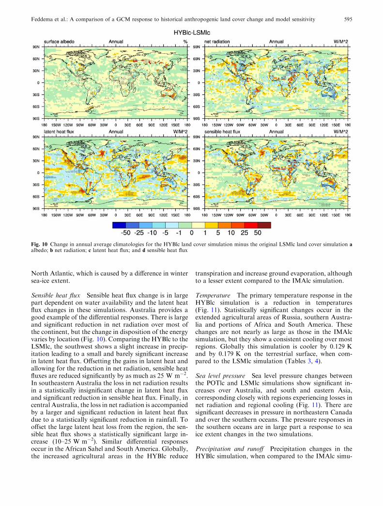
Sensible heat flux Sensible heat flux change is in largepart dependent on water availability and the latent heatflux changes in these simulations. Australia provides agood example of the differential responses. There is largeand significant reduction in net radiation over most ofthe continent, but the change in disposition of the energyvaries by location (Fig. 10). Comparing the HYBlc to theLSMlc, the southwest shows a slight increase in precip-itation leading to a small and barely significant increasein latent heat flux. Offsetting the gains in latent heat andallowing for the reduction in net radiation, sensible heatfluxes are reduced significantly by as much as 25 W m�2.In southeastern Australia the loss in net radiation resultsin a statistically insignificant change in latent heat fluxand significant reduction in sensible heat flux. Finally, incentral Australia, the loss in net radiation is accompaniedby a larger and significant reduction in latent heat fluxdue to a statistically significant reduction in rainfall. Tooffset the large latent heat loss from the region, the sen-sible heat flux shows a statistically significant large in-crease (10–25 W m�2). Similar differential responsesoccur in the African Sahel and South America. Globally,the increased agricultural areas in the HYBlc reduce

transpiration and increase ground evaporation, althoughto a lesser extent compared to the IMAlc simulation.

Temperature The primary temperature response in theHYBlc simulation is a reduction in temperatures(Fig. 11). Statistically significant changes occur in theextended agricultural areas of Russia, southern Austra-lia and portions of Africa and South America. Thesechanges are not nearly as large as those in the IMAlcsimulation, but they show a consistent cooling over mostregions. Globally this simulation is cooler by 0.129 Kand by 0.179 K on the terrestrial surface, when com-pared to the LSMlc simulation (Tables 3, 4).

Sea level pressure Sea level pressure changes betweenthe POTlc and LSMlc simulations show significant in-creases over Australia, and south and eastern Asia,corresponding closely with regions experiencing losses innet radiation and regional cooling (Fig. 11). There aresignificant decreases in pressure in northeastern Canadaand over the southern oceans. The pressure responses inthe southern oceans are in large part a response to seaice extent changes in the two simulations.

Precipitation and runoff Precipitation changes in theHYBlc simulation, when compared to the IMAlc simu-

Fig. 10 Change in annual average climatologies for the HYBlc land cover simulation minus the original LSMlc land cover simulation aalbedo; b net radiation; c latent heat flux; and d sensible heat flux

Feddema et al.: A comparison of a GCM response to historical anthropogenic land cover change and model sensitivity 595

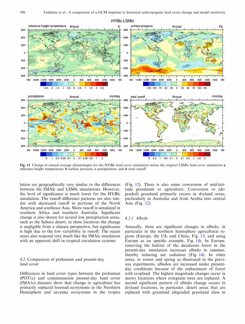
lation are geographically very similar to the differencesbetween the IMAlc and LSMlc simulations. However,the level of significance is much lower for the HYBlcsimulation. The runoff difference patterns are also sim-ilar with decreased runoff in portions of the NorthAmerica and southeast Asia. More runoff is simulated insouthern Africa and southern Australia. Significantchange is also shown for several low precipitation areas,such as the Sahara desert, in these locations the changeis negligible from a climate perspective, but significanceis high due to the low variability in runoff. The oceanareas also respond very much like the IMAlc simulationwith an apparent shift in tropical circulation systems.

4.2 Comparison of prehuman and present-dayland cover

Differences in land cover types between the prehuman(POT1c) and commensurate present-day land cover(IMA1c) datasets show that change to agriculture hasprimarily replaced forested ecosystems in the NorthernHemisphere and savanna ecosystems in the tropics

(Fig. 12). There is also some conversion of mid-lati-tude grasslands to agriculture. Conversion to (de-graded) grassland primarily occurs in dryland areas,particularly in Australia and from Arabia into centralAsia (Fig. 12).

4.2.1 Albedo

Annually, there are significant changes in albedo, inparticular in the northern hemisphere agricultural re-gions (Europe, the US, and China, Fig. 13; and usingEurope as an specific example, Fig. 14). In Europe,removing the leafout of the deciduous forest in thepresent-day simulation increases albedo in summer,thereby reducing net radiation (Fig. 14). In otherareas, in winter and spring as illustrated in the previ-ous experiments, albedos are increased under present-day conditions because of the replacement of forestwith cropland. The highest magnitude changes occur insnowy locations where evergreen trees are replaced. Asecond significant pattern of albedo change occurs indryland locations, in particular, desert areas that arereplaced with grassland (degraded grassland class in

Fig. 11 Change in annual average climatologies for the HYBlc land cover simulation minus the original LSMlc land cover simulation areference height temperature; b surface pressure; c precipitation; and d total runoff

596 Feddema et al.: A comparison of a GCM response to historical anthropogenic land cover change and model sensitivity

IMAGE 2.2) tend to have a large reduction in albedo(e.g., Saudi Arabia, the central western US, andsoutheastern Australia; Fig. 7).

4.2.2 Solar radiation

As shown by the European example (Fig. 14), loss of netradiation is not only a function of albedo, but also dueto a reduction in incident solar radiation. Incidentradiation is also significantly reduced over otherNorthern Hemisphere agricultural areas and to a lesserextent over the Congo basin (not statistically significant)and the agricultural region of northern Argentina and

Paraguay (Fig. 13). In the Sahel and Central Australia,there are significant and large increases in incidentradiation. Changes in incident radiation cannot be ex-plained by surface energy balance differences and sug-gest that other model feedbacks play a role in theobserved climate changes.

Reviewing the changes in cloud cover, it is apparentthat a significant portion of the net radiation change canbe explained by the cloud feedbacks in the simulations(Fig. 13). In summer (JJA), both North America andEurope experience significant change in total cloudcover (>10%). This reduces incident solar radiation tothese regions and hence net radiation (Fig. 15). Similar

Fig. 12 Replaced land covertypes due to human activitiesbased on the IMAGE 2.2present-day and potentialvegetation land cover landcover datasets: a natural landcover types converted toagriculture; and b natural landcover types converted tograssland

Feddema et al.: A comparison of a GCM response to historical anthropogenic land cover change and model sensitivity 597

strong increases in cloud cover are observed in theSouthern Hemisphere during the winter (JJA), especiallyover southwestern Africa and portions of South Amer-ica. Clouds increase over the northern tropical PacificOcean, indicating a potential shift in the ITCZ over thisregion. In DJF increases in cloud cover are found in thesoutheastern US and southwestern Australia. There arealso a number of regions that experience decreases incloud cover in the present-day (IMAlc) simulations.Most significant is north central Australia, SE Asia, theSahel, the tropical Pacific Ocean; and Southern Africa insummer (DJF).

Because of the changes in albedo and cloud cover, netradiation is significantly reduced on a global scale(Fig. 15; Tables 3, 4). However, regionally and season-ally these changes are highly variable. The spring andsummer seasons show very significant reductions in netradiation in the mid latitudes (not shown, but similar tothe IMAlc and LSMlc simulation comparisons). Theareas most affected are the agricultural areas of easternNorth America, western Europe, China and easternAustralia, as well as smaller areas in eastern SouthAfrica and eastern South America. Dryland areas con-verted to agriculture or grassland, mostly in the tropicsand subtropics, show marked increases in net radiation

during the growing season. On average, net radiation isreduced by 0.662 W m�2 globally and by 1.46 W m�2

terrestrially.

4.2.3 Latent heat flux

Changes in latent heat flux are generally greatest in themid-latitude spring and summer seasons due toreductions in net radiation (Fig. 15; seasonal plots notshown but the effects are similar to those in the IMAlcand LSMlc comparison). Declines are less significantin the summer and especially so in fall when manylocations experience reduced soil moisture conditions,resulting in little change in evapotranspiration rates.However, there are some notable exceptions in thistrend. For example, in northeastern Mexico and Texas,because of increases in local precipitation in spring andsummer, latent heat flux is increased in late summer.In parts of southwestern Australia and in the westernUS, the increased transpiration efficiency of crops alsoincreases latent heat fluxes in these locations, particu-larly in the summer when there is an accompanyingincrease in precipitation (see discussion on precipita-tion). Several other areas, particularly where agricul-

Fig. 13 Change in annual average climatologies for the present-day IMAlc land cover simulation minus the POTlc land cover simulation:a albedo; b incident radiation; c total cloud cover (DJF); and d total cloud cover (JJA)

598 Feddema et al.: A comparison of a GCM response to historical anthropogenic land cover change and model sensitivity

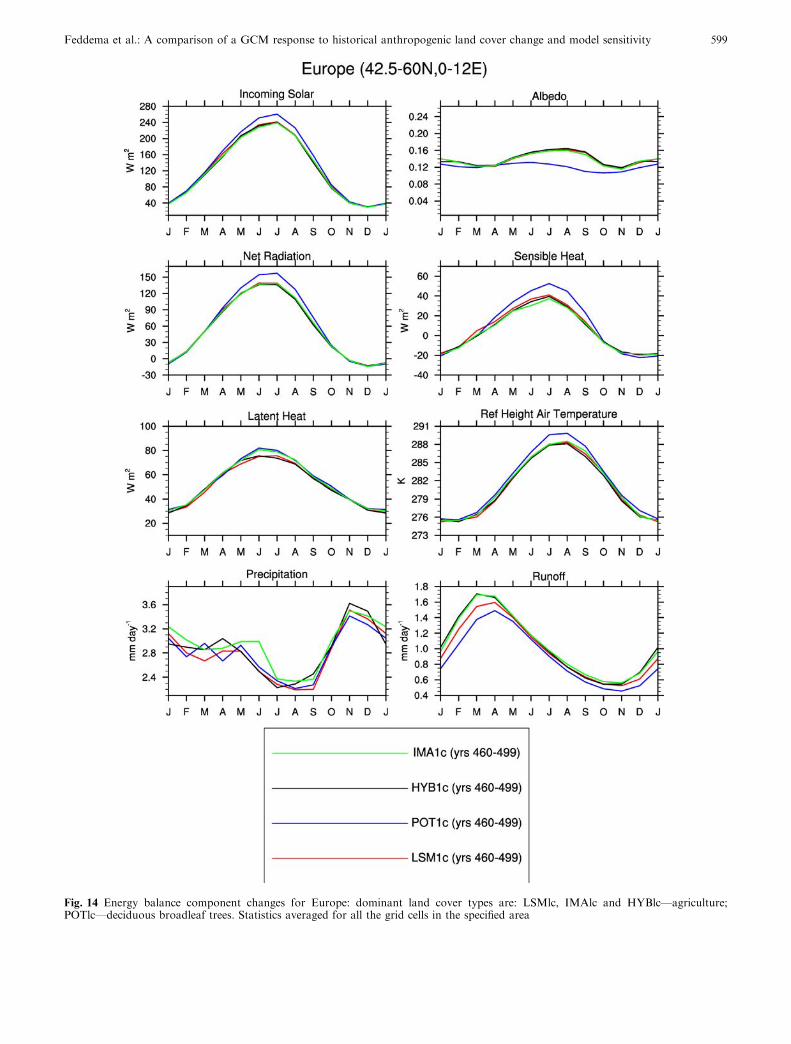
Fig. 14 Energy balance component changes for Europe: dominant land cover types are: LSMlc, IMAlc and HYBlc—agriculture;POTlc—deciduous broadleaf trees. Statistics averaged for all the grid cells in the specified area

Feddema et al.: A comparison of a GCM response to historical anthropogenic land cover change and model sensitivity 599

ture has been introduced in China, southeastern por-tions of South America (northern Argentina) andAustralia similarly have increased latent heat fluxes

due to precipitation increases. North central Australia,experiences significant decreases in latent heat flux as aresult of decreased rainfall over this region, accompa-

Fig. 15 Change in annualaverage climatologies for thepresent-day IMAlc land coversimulation minus the POTlcland cover simulation: a netradiation; b latent heat flux; csensible heat flux

600 Feddema et al.: A comparison of a GCM response to historical anthropogenic land cover change and model sensitivity

nying the reduced cloud cover conditions in the pres-ent-day simulation. Some statistically significant chan-ges are in locations where dryland surfaces have beenvegetated to degraded grasslands (e.g., desert tograssland in Saudi Arabia). However, while statisticallysignificant, these changes are very small in magnitude.

On the terrestrial surface, latent heat flux absorbsabout half the loss in net radiation (�0.714 W m�2;Table 4). Globally this value is reduced to�0.599 W m�2, which comprises the majority of theglobal change in net radiation (�0.662 W m�2; Ta-ble 3). This indicates that there is a significant decreasein latent heat flux over the ocean surface as a wholealthough there are areas with significant increases inevaporation and latent heat flux, such as the westernIndian Ocean, south of Australia and, to a lesser extent,off the west coast of North America. In addition, thedecreased area of forest and increased agriculture, with aharvest cycle, reduced global LAI resulting in reducedtranspiration and canopy evaporation (about 1 W m�2

total) only slightly offset by about 0.2 W m�2 increase inground evaporation (Table 4).

4.2.4 Sensible heat flux

The overall magnitude of the sensible heat flux responseis similar to the latent heat flux responses on land(�0.744 W m�2), while on a global scale this change isgreatly reduced (�0.048 W m�2), and makes up a muchsmaller proportion of the net radiation loss (Fig. 15;Tables 3, 4). Statistically, these changes are of greatersignificance compared to the latent heat flux changes,especially over land. As with latent heat flux, in mostlocations the changes are negative and are especiallyevident during the crop-growing season where naturalland cover has been replaced with agriculture. Mostnotable are the extensive reductions in sensible heat fluxover the agricultural areas of eastern North America,Europe and China and South America. However in thetropics there are a number of less extensive, but statis-tically significant, increases in sensible heat flux. Exam-ples are over the southeastern Amazon and southeastAsia where agriculture replaces tropical forest and in thedesert fringes of Africa, and central Australia wheregrasslands replace desert and shrublands. Several oceanareas also demonstrate statistically significant sensibleheat flux responses. All the ocean areas downwind frommajor mid latitude agricultural regions show increasedsensible heat releases, especially in winter (i.e., down-wind from the eastern US, China, and to a lesser extentSouth America and Australia).

4.2.5 Temperature

The annual temperature differences between the IMAlcand POTlc show that the present-day climate is coolerover most the globe (Fig. 16), with a global averagetemperature reduction of 0.386 and 0.54 K for the ter-

restrial surface (Tables 3, 4). This trend is statisticallysignificant over most of the planet in the traditionaldifference of the mean test. Using the bootstrappingtechnique to eliminate temporal and spatial correlations,the significance regions are greatly reduced and are al-most exclusively limited to terrestrial areas (contoursshow the 95% confidence level based on the bootstrapmethodology). Regionally the greatest cooling coincideswith areas that have been converted from natural forestvegetation to agriculture or grasslands in mid-latitudes.Within these areas, central and east Asia stand out asstatistically most significant for both statistical tests.Europe also shows statistical significance for both tests,although not the entire area is statistically significant inthe annual time frame. Other small patches of land useconversion are statistically significant by the bootstrapmethodology even though they do not translate intocohesive large areas of change (e.g., east Australia coast,South America and southern Africa and Ethiopia).Numerically the largest cooling is observed over theArctic, but this is not statistically significant by thebootstrap statistics.

Although not statistically significant by the conser-vative bootstrap measure, there are also a few areaswhere there is a systematic warming on an annual scaleand significant on the standard t test significance sta-tistic. Terrestrially, these areas are all linked to land useconversion representing either tropical forest conversionto agriculture in the Amazon and Venezuela as well asan isolated grid cell over Sumatra. In addition, thecentral Australian continent is warmer due to reducedwater resources for latent heat fluxes. Although notstatistically significant by either test, areas around theBlack Sea and western North America, converted fromgrassland to agriculture, show a slight warming insummer. While there are large changes in temperature ofthe polar ocean areas, these changes are generally notsignificant because of the high temperature variability,and are associated with changes in sea-ice concentra-tions of up to 15 percent (e.g., North Atlantic and southof Cape Horn).

There are marked seasonal differences in the magni-tude and location of cooling. These trends are related tothe type of land cover conversion and are strongly cor-related with the summer season. In JJA (Fig. 16), thereis a very strong cooling signal across most of theNorthern Hemisphere mid-latitudes, with most statisti-cally significant areas in the Northern Hemisphere.Especially strong are the cooling trends over the south-ern and southeastern US, the Mediterranean area andMongolia. The areas of significant change shift to theSouthern Hemisphere during DJF in the agriculturalregions of South America, South Africa and southeast-ern Australia. Compared to the Northern Hemisphere,these areas are much smaller in extent due to the limitedland area. The tropics show small patches of change,also seasonally differentiated especially in Africa,southeastern Asia and northern Australia. These chan-ges are small because there is relatively little change in

Feddema et al.: A comparison of a GCM response to historical anthropogenic land cover change and model sensitivity 601

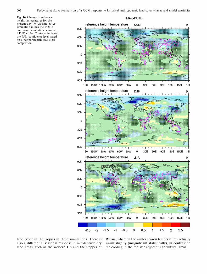
land cover in the tropics in these simulations. There isalso a differential seasonal response in mid-latitude dryland areas, such as the western US and the steppes of

Russia, where in the winter season temperatures actuallywarm slightly (insignificant statistically), in contrast tothe cooling in the moister adjacent agricultural areas.

Fig. 16 Change in referenceheight temperatures for thepresent-day IMAlc land coversimulation minus the POTlcland cover simulation: a annual;bDJF; c JJA. Contours indicatethe 95% confidence level basedon a nonparametric statisticalcomparison

602 Feddema et al.: A comparison of a GCM response to historical anthropogenic land cover change and model sensitivity

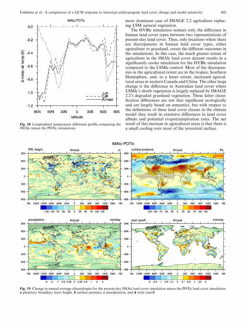
Much of the observed cooling is due to a significantreduction of the mean maximum daily temperaturecentered over the main agricultural regions of the globe(Fig. 17). In Europe and parts of North America, thisreduction is offset by a slight, but insignificant, rise indaily minimum temperatures (Fig. 17), thus reducing thediurnal temperature range in these two areas. Increasedtemperatures in the tropical regions are primary the re-sult of insignificant increases in both maximum andminimum temperatures. The diurnal range in tempera-ture increases in a few dry desert areas over the SouthernSahara extending to the Arabian Peninsula and overcentral Australia. All these regions are affected by theITCZ, and all experience a drying and heating. The ex-tents of the tropical changes are very minor, and, over-all, this experiment predicts cooling over all latitudezones (Fig. 18). Zonally, these changes range from de-creases of 0.2 K at the equator to about 1.0 K in theArctic.

The difference in the bootstrap and t test significancetests is very large in the example. We believe that the ttest is very liberal—it will produce false positive resultsfor roughly 5% of the grid cells. Moreover, due to thepositive spatial correlation of the fields the significantcell grid will be spatially clustered. The bootstrap testbased on the maximum Z score is quite conservative.For example, at the 0.05 level 95% of the time there willbe no grid cells that are identified as significant. So evena single grid cell being deemed significant based on themaximum is unusual. Having approximately 5% of thebootstrap/maximum test grid cells significant in thisexample is a coincidence.

4.2.6 Planetary boundary layer

The reduced temperatures and a general reduction insurface roughness as forests are replaced by agricultureand shrub and semi desert vegetation with grasslandsresults in a general lowering of the boundary layerheight (Fig. 19). The warming over the Sahel and centralAustralia lead to significant increases in the PBL in thoseareas.

4.2.7 Planetary boundary layer and sea level pressure

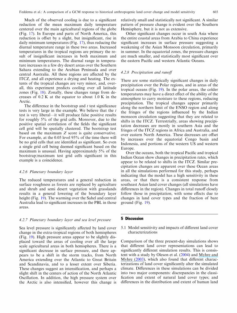
Sea level pressure is significantly affected by land coverchange in the extra-tropical regions of both hemispheres(Fig. 19). High pressure areas appear to be slightly dis-placed toward the areas of cooling over all the largescale agricultural areas in both hemispheres. There is asignificant decrease in surface pressure, and there ap-pears to be a shift in the storm tracks, from NorthAmerica extending over the Atlantic to Great Britainand Scandinavia, and to a lesser extent over Siberia.These changes suggest an intensification, and perhaps aslight shift in the centers of action of the North AtlanticOscillation. In addition, the high pressure system overthe Arctic is also intensified, however this change is

relatively small and statistically not significant. A similarpattern of pressure change is evident over the SouthernHemisphere, but it is not as extensive.

Other significant changes occur in south Asia wherethe entire coastal areas from Arabia to China experiencesignificant increases in surface pressure suggesting aweakening of the Asian Monsoon circulation, primarilyin summer. In the equatorial zones, the pressure changesare much smaller, and statistically most significant overthe eastern Pacific and western Atlantic Oceans.

4.2.8 Precipitation and runoff

There are some statistically significant changes in dailyprecipitation over the Polar regions, and in areas of thetropical oceans (Fig. 19). In the polar areas, the coldertemperatures may have a direct effect of the ability of theatmosphere to carry moisture to these regions, reducingprecipitation. The tropical changes appear primarilyalong the northern limit of the ENSO region and alongthe fringes of the regions influenced by the Indianmonsoon circulation suggesting that they are related toshifts in the ITCZ. Terrestrially, areas showing precipi-tation decreases are mostly in southern Asia and thefringes of the ITCZ regions in Africa and Australia, andover eastern North America. These decreases are offsetby increases over the equatorial Congo basin andIndonesia, and portions of the western US and westernEurope.

Over the oceans, both the tropical Pacific and tropicalIndian Ocean show changes in precipitation rates, whichappear to be related to shifts in the ITCZ. Similar pre-cipitation changes are apparent over these Ocean areasin all the simulations performed for this study, perhapsindicating that the model has a high sensitivity in theseareas, or that there is a consistent response fromsoutheast Asian land cover changes (all simulations havedifferences in the region). Changes in total runoff closelyfollow those in precipitation, with some effects due tochanges in land cover types and the fraction of bareground (Fig. 19).

5 Discussion

5.1 Model sensitivity and impacts of different land covercharacterizations

Comparison of the three present-day simulations showsthat different land cover representations can lead tosignificantly different simulation results. This is consis-tent with a study by Oleson et al. (2004) and Myhre andMyhre (2003), which also found that different charac-terizations of land cover significantly alter the simulatedclimate. Differences in these simulations can be dividedinto two major components: discrepancies in the classi-fication and extent of natural land cover types; anddifferences in the distribution and extent of human land

Feddema et al.: A comparison of a GCM response to historical anthropogenic land cover change and model sensitivity 603

cover types. Comparing the simulations in this projectallows us to evaluate the impacts of both of these dif-ferences.

Comparing the IMAlc and LSMlc simulations showsthe combined impacts of human and natural vegetationdifferences. Besides other locations, the Siberian arcticand Amazon regions illustrate that there are significantdifferences in simulated climates because of natural landcover classification discrepancies between datasets. Inthe Siberian region, albedo changes result in impacts onall aspects of climate, with a net result of the IMAlcsimulation having a statistically significant higher aver-age annual temperature compared to the LSMlc simu-lation. The change in latent heat flux is relatively smallbecause in summer this environment is water limited. Asa result, most of the net radiation increase is dissipated

as sensible heat flux, in turn leading to the temperatureincrease. In the Amazon, changing land cover fromevergreen tropical forest to deciduous tropical forestalso results in a warmer climate in the IMAlc simulation.In this case, the warming is primarily due to changes inevapotranspiration rates. The reduced disposition ofenergy from the surface by latent heat flux results in awarmer surface and an increase in sensible heat fluxvalues.

In most instances, when croplands replace forests thistypically leads to increased albedos and cooling, whilechange from natural dryland vegetation types to agri-culture result in warming. Significant cooling is the re-sult in southwestern Australia where LSMlc mixedforest-agriculture and shrub vegetation are replaced bygrasslands in the IMAlc simulation; a reversal of the

Fig. 17 Change in a averageminimum and b maximumreference height temperaturefor the present-day IMAlc landcover simulation minus thePOTlc land cover simulation

604 Feddema et al.: A comparison of a GCM response to historical anthropogenic land cover change and model sensitivity

more dominant case of IMAGE 2.2 agriculture replac-ing LSM natural vegetation.

The HYBlc simulation isolates only the difference inhuman land cover types between two representations ofpresent-day land cover. Thus, only locations where thereare discrepancies in human land cover types, eitheragriculture or grassland, create the different outcomes inthe simulations. In this case, the much greater extent ofagriculture in the IMAlc land cover dataset results in asignificantly cooler simulation for the HYBlc simulationcompared to the LSMlc control. Most of the discrepan-cies in the agricultural extent are in the tropics, SouthernHemisphere, and, to a lesser extent, increased agricul-tural areas in western Canada and China. The other largechange is the difference in Australian land cover whereLSMlc’s shrub vegetation is largely replaced by IMAGE2.2¢s degraded grassland vegetation. These latter classi-fication differences are not that significant ecologicallyand are largely based on semantics, but with respect tothe definitions of these land cover classes in the climatemodel they result in extensive differences in land coveralbedo and potential evapotranspiration rates. The netresult of this increase in agricultural areas is that there isa small cooling over most of the terrestrial surface.

Fig. 18 Longitudinal temperature difference profile comparing theIMAlc minus the POTlc simulations

Fig. 19 Change in annual average climatologies for the present-day IMAlc land cover simulation minus the POTlc land cover simulation:a planetary boundary layer height, b surface pressure, c precipitation, and d total runoff

Feddema et al.: A comparison of a GCM response to historical anthropogenic land cover change and model sensitivity 605

Overall, the IMAGE 2.2 land cover database resultsin a warmer global climate simulation compared to theNCAR LSM land cover dataset. Most of this warming isthe result of discrepancies in the distribution of naturalvegetation types. However, as shown by the Hybrid landcover simulation, cooling due to the differences in agri-cultural extent largely offsets this warming. These biasesshould be taken into consideration when selecting aparticular dataset for simulating land cover change in aGCM.

5.2 Historical climate impacts of human induced landcover change

5.2.1 Global impacts

Historical human land cover change is simulated to havea 0.39 K cooling effect on global temperatures and0.54 K over the terrestrial surface. There are severalnotable characteristics associated with these changes.The reduction in global average net radiation is about0.66 W m�2, latent heat flux decreases by 0.60 W m�2

and sensible heat flux is reduced by 0.05 W m�2. Thesechanges are much larger over the terrestrial surface, witha reduction of 1.46 W m�2 in net radiation, which ismore evenly partitioned between latent and sensible heatflux reductions (0.74 W m�2 and 0.71 W m�2 respec-tively). These values are approximately double themaximum observed range between the different present-day land cover simulations, which in this context can bethought of as an uncertainty measure.

There are also significant differences in the seasonal-ity of the prehuman and present-day simulations. Theboreal summer (JJA) sees a much greater portion of thenet radiation reduction (0.726 W m�2), leading to a0.64 W m�2 reduction in latent heat fluxes and a0.21 W m�2 reduction in sensible heat fluxes globally. Incomparison, the boreal winter (DJF) sees a 0.34 W m�2

net radiation reduction, which, combined with a drying,creates a 0.56 W m�2 reduction in latent heat flux and a0.246 W m�2 increase in sensible heat flux globally.

Our simulated �0.39 K globally temperature changecan be compared to a number of previously reportedglobal values. In a study with essentially the sameatmospheric model, but with slab oceans, Govindasamyet al. (2001) reported a �0.25 K global temperaturechange. Using the HadAM3 with prescribed Oceanconditions Betts observed a �0.25 K temperaturechange, and Hansen et al. (1998) reported �0.14 K forthe GISS model. Results from intermediate complexitymodels found global temperature changes of �0.35 Kfor the biogeophysical experiment by Brovkin et al.(1999), and �0.13 K by Matthews et al. (2003). Zon-ally, we find a minimum �0.2 K change over the tro-pics to a maximum �1.0 K over the arctic. Thiscompares to reported zonal cooling from 0.09 K in thetropics to 0.22 K in the mid latitudes of the NorthernHemisphere by Matthews et al., (2003); and a warming

of 0.8 K in the tropics and cooling of 0.7–1.1 K in theNorthern Hemisphere mid latitudes reported by Bou-noua et al. (2002). In all cases there is agreement on anoverall cooling of global temperatures. Reported resultsdiffer in part because they use different representationsof land cover and because of differences in the GCMsand the experimental set-ups. These results suggest thatthe NCAR LSM may be more sensitive to land coverchange in comparison to other models, while the PCMis known to have a low sensitivity to greenhouse gaseffects. Furthermore, our findings of a greater coolingin this fully coupled simulation, compared to forexample Govindasamy et al. (2001), suggest that thereare potentially significant ocean-atmosphere feedbacksthat accompany the historical impacts of land coverchange.

5.2.2 Regional impacts

Compared to the global statistics, regional changes be-tween the simulations are much larger, up to 2 K,especially over areas converted to agriculture. In thiscontext, the global statistics can be deceptive becausethey ignore the regional impacts of land cover changeeffects, which are often offsetting on a global scale.Notable in these simulations is that all the major agri-cultural regions of the globe (eastern US, Europe, Chi-na, mid latitudes of South America, South Africa andsoutheastern Australia) show significant cooling. Thesemid-latitude cooling trends are strongly associated withthe summer season, but persist in winter. Dryland re-gions converted to agriculture have a slightly differentresponse to converted wetter areas, in part because thelimited water supply cannot be used to compensate foralbedo induced net radiation change through latent heatflux changes.

Other regions that are significantly affected in thissimulation are southeast and eastern Asia, which show avery strong cooling year round. In addition, precipita-tion is also decreased in most of these areas, althoughthis trend is not as statistically significant. Also affectedare the dryland areas of Africa and Australia, where thedesert margins, largely controlled by ITCZ rainfall re-gimes, show a considerable drying and warming. Al-though these signals are consistent, they are generallynot statistically significant. There are also very slight,insignificant, increases in Tropical precipitation overAfrica and Indonesia.

5.2.3 Mechanisms of climate change due to land cover

The differences in the historical and present-day climatesimulations show a distinct pattern of change. In gen-eral, the mid-latitude cooling over the agricultural re-gions leads to strong cooling that is initiated throughchanges in the surface energy balances in the region.Conversion to agriculture from forest in particular leads

606 Feddema et al.: A comparison of a GCM response to historical anthropogenic land cover change and model sensitivity

to significant albedo change and reductions in net radi-ation. However, there is also an apparent positivefeedback that leads to additional cloud cover and fur-ther cooling, especially evident over Europe and easternNorth America. As the pressure difference map indi-cates, there is an eastward shift and intensification of thezonal pressure patterns (Fig. 19). This preliminaryanalysis suggests there is a significant increase in zonalflow (not shown) and a shifting and perhaps intensifi-cation of regional storm tracks.

The other large scale change is in southern andeastern Asia. These areas show some of the most sig-nificant cooling all along the continental fringe. Thiscooling appears to have a direct impact on the monsooncirculation. Especially in the summer, the cooling of theland surface weakens the monsoon circulation leading toless onshore flow, reducing precipitation over the region.In turn the monsoon flows alter the location, and ap-pears to reduce, the migration extent of the ITCZ,especially over eastern Africa and Australia. Both re-gions experience decreased cloud cover and drying.

While this study cannot specifically identify the tim-ing of these regional climate changes, they should followperiods of land cover conversion. For Europe, thiswould be the period from 1,200 to about 1,700 (Goudie1990), potentially linking land use change to little ice ageconditions as proposed by Govindasamy et al. (2001). InNorth America the timing of deforestation is primarilyfrom the mid 1700s to the early 1900s (Goudie 1990).Other regions would have experienced such change morerecently, possibly influencing the 20th century climaterecord. In this study, the observed cooling is primarilythrough a reduction in daily maximum temperatures.Karl et al. (1993) showed that in the US there was ageneral rising trend in temperatures, with most warmingcoming from rising minimum temperatures. This ob-served trend is compatible with the results from thisstudy if a land cover cooling occurred at the same timeas a warming trend from other forcings (e.g., GHGs; seeBonan 2001). The greater warming effects cancel thecooling trend of the daily maximum temperatures whilethe minimal change in daily minimum temperatures dueto land cover change does not affect the overall warmingtrend. Observations reported by the IPCC (2001) indi-cate that the daily temperature range is decreasing inmany other regions of the Earth, especially southeastAsia as is simulated in this study.

6 Conclusions

Human induced land cover change is potentially animportant factor in regional and global climate change,and studies of past human land cover change couldimprove our understanding of historical climate change.This study and most historical land cover change studiesshow that past land cover change has led to globalcooling. The mechanisms for cooling are twofold. Firstthere is a direct cooling effect due to albedo changes in

mid-latitudes. Second, there is an indirect effect coolingdue to feedbacks in mid-latitude and Asian monsooncirculation systems that result in increased cloud coverconditions. However, future land cover scenarios willnot necessarily result in additional cooling becauseadditional agricultural lands in the future would begin toreplace more dryland areas and tropical forests, ascompared to replacing mid-latitude forest areas in thepast. It has been shown by DeFries et al. (2002) that the2050 IMAGE land cover projections could result inwarming. This may hold true for this model, but becauseof the small areas affected in this study it cannot beshown statistically. This signal switch between past andfuture effects of land cover change could be an impor-tant contributor to recent observed temperature trends.

We conclude with the answers to the questions posedat the outset of this paper:

1. What is the sensitivity of a fully coupled generalcirculation model to different present-day land coverrepresentations?

The DOE-PCM shows a significant sensitivity todifferent representations of present-day land coverchange with simulation outcomes ranging by 0.21 K inglobal mean annual surface air temperature. Further-more, historical land cover change could have cooledglobal average temperatures by about 0.39 K and, per-haps of greater importance, regionally up to 2 K.Therefore, it is clear that land cover representation is animportant consideration in GCM simulations, especiallyon the regional level. In addition, in order to compareland cover change studies across GCMs it is importantthat a consistent land cover change treatment be used.

2. What is the best method for including alternativeland cover scenarios into GCM simulations?

If land cover simulations are to be used in climatechange scenario simulations, the hybrid methodologyused in this paper, and also used by De Fries et al.(2002), would be the most appropriate methodology forincorporating land cover change into different GCMs.Most models have been calibrated based on their nativeland cover classification schemes (LSMlc in this case).This methodology allows all models to use similar rep-resentation of anthropogenic land cover change, whileminimizing differences between the natural vegetationclasses of comparable alternative model simulations.

3. Within the context of the uncertainty associated withrepresenting present-day land cover, could historicalhuman land cover change have had a significant im-pact on climate? Is this signal sufficiently large tosuggest the need for including land cover change aspart of IPCC based future climate scenarios?

In this paper, the change in global temperature fromprehuman vegetation conditions to present-day condi-

Feddema et al.: A comparison of a GCM response to historical anthropogenic land cover change and model sensitivity 607

tions is roughly twice the magnitude (�0.39 K) of thatresulting from contrasts in present-day simulations(0.21 K). This is about one third the projected 20thcentury warming due to GHG, aerosol, volcanic andsolar forcing in the DOE-PCM (Meehl et al. 2003, 2004).More important, however, is that the largest impacts ofland cover change (�2 K) are observed on regionalscales. In these areas changes due to land cover con-version are comparable to those due to other simulatedforcings (Meehl et al. 2003, 2004). In many cases thesesignificant regional changes also coincide with regions ofhighest human population and potential climate impactson society. This suggests that land cover change doeshave a significant role in producing global and regionalclimate changes that could impact large sections of thehuman population. Therefore, land cover change shouldbe used in historical and future SRES climate scenariosimulations.

4. Are global statistics adequate to detect climate signalsfrom land cover change? Is there a discernable spatialpattern associated with land cover induced climatechange?

Global or terrestrial average climate statistics do notgive a good representation of the effects of land coverchange on climate. The effects of land cover change arehighly regional and are largely offsetting on a globalscale. This work supports the hypothesis from previouswork that conversion of forested land to agriculture inthe mid latitudes leads to significant cooling over theseregions and a reduction in diurnal temperature ranges.In addition, feedbacks that increase cloud cover andreductions in solar radiation amplify this cooling trend.There is some evidence that tropical land cover con-version may lead to warming signals, but the small areasinvolved in this experiment provide insufficient evidence.This experiment also suggests that land cover change inAsia may have a significant impact on the Asian Mon-soon circulation and in turn the extent of the ITCZ overthe Indian and Pacific Oceans.

Acknowledgements Special thanks to Rik Leemans for providingthe SRES data, and Tom Bettge and Lawrence Buja for theirassistance in running the experiments, and two anonymousreviewers for their comments and suggestions. This research wassupported by the Office of Science (BER), US Department of En-ergy, Cooperative Agreement No. DE-FC02-97ER62402, the Na-tional Science Foundation grant numbers ATM-0107404, andATM-0413540, the NCAR Weather and Climate Impact Assess-ment Science Initiative funded by NSF, and the University ofKansas, Center for Research.

References

Alcamo J (ed) (1994) IMAGE 2.0: integrated modeling of globalclimate change. Kluwer, Dordrecht, pp 318

Alcamo J, Leemans R, Kreileman E (eds) (1998) Global changescenarios of the 21st century. Results from the IMAGE 2.1model. Pergamon, London, pp 296

Ammann CM, Meehl GA, Washington WM, Zender CS (2003) Amonthly and latitudinally varying volcanic forcing dataset insimulations of 20th century climate. Geophys Res Lett30(12):1657, DOI 10.1029/2003GL016875

Avissar R (1995) Recent advances in the representation of land-atmosphere interactions in general circulation models. RevGeophys 33:1005–1010, DOI 10.1029/95RG00258

Betts RA (2001) Biogeophysical impacts of land use on present-dayclimate: near-surface temperature and radiative forcing. AtmosSci Lett 2: 39–51, DOI 10.1006/asle.2001.0023

Bonan G (1994) Comparison of two land surface models usingprescribed forcings. Journal of Geophysical

Bonan GB (1996) A land surface model (LSM version 1.0) forecological, hydrological, and atmospheric studies: technicaldescription and user¢s guide. NCAR Technical Note NCAR/TN-417+STR. National Center for Atmospheric Research,Boulder, Colorado, pp 150

Bonan GB (1997) Effects of land use on the climate of the UnitedStates. Clim Change 37:449–486. DOI 10.1023/A:1005305708775

Bonan GB (1998) The land surface climatology of the NCAR landsurface model coupled to the NCAR Community ClimateModel. J Clim 11(6):1307–1326. DOI 10.1175/1520–0442(1998)011<1307

Bonan GB (1999) Frost followed the plow: impacts of deforestationon the climate of the United States. Ecol Appl 9(4):1305–1315

Bonan GB (2001) Observational evidence for reduction of dailymaximum temperature by croplands in the Midwest UnitedStates. J Clim 14(11):2430–2442. DOI 10.1175/1520–0442(2001)014<2430

Bonan GB, Oleson KW, Vertenstein M, Levis S, Zeng X, Dai Y,Dickinson RE, Yang Z (2002) The land surface climatology ofthe community land model coupled to the NCAR CommunityClimate Model. J Clim 15(22):3123–3149. DOI 10.1175/1520–0442(2002)015<3123

Boone A, Habets F, Noilhan J, Clark D, Dirmeyer P, Fox S, GusevY, Haddeland I, Koster R, Lohmann D, Mahanama S, MitchellK, Nasonova O, Niu G-Y, Pitman A, Polcher J, Shmakin AB,Tanaka K, van den Hurk B, Verant S, Verseghy D, Viterbo P,Yang Z-L (2004) The Rho ne-aggregation land surface schemeintercomparison project: an overview. J Clim 17(1):187–208.DOI 10.1175/1520–0442(2004)017<0187

Bounoua LR, DeFries R, Collatz GJ, Sellers P, Khan H (2002)Effects of land cover conversion on surface climate. ClimChange 52:29–64. DOI 10.1023/A:1013051420309

Brovkin V, Ganopolski A, Claussen M, Kubatzki C, Petoukhov V(1999) Modelling climate response to historical land coverchange. Global Ecology and Biogeography 8:509–517

Chase TN, Peilke Sr. RA, Kittel TGF, Nemani RR, Running SW(2000) Simulated impacts of historical land cover changes onglobal climate in northern winter. Clim Dyn 16(2–3):93–105.DOI 10.1007/s003820050007

Chen TH, Henderson-Sellers A, Milly PCD, Pitman AJ, BeljaarsACM, Polcher J, Abramopoulos F, Boone A, Chang S, Chen F,Dai Y, Desborough C E, Dickinson RE, Du menil L, Ek M,Garratt JR, Gedney N, Gusev YM, Kim J, Koster R, Kow-alczyk EA, Laval K, Lean J, Lettenmaier D, Liang X, MahfoufJ-F, Mengelkamp H-T, Mitchell K, Nasonova ON, Noilhan J,Robock A, Rosenzweig C, Schaake J, Schlosser CA, Schulz J-P,Shao Y, Shmakin AB, Verseghy DL, Wetzel P, Wood EF, XueY, Yang Z-L, Zeng Q (1997) Cabauw experimental results fromthe project for intercomparison of land-surface parameteriza-tion schemes. J Clim 10(6):1194–1215. DOI 10.1175/1520–0442(1997)010<1194

Claussen M, Brovkin V, Ganapolski A (2001) Biogeophysicalversus biogeochemical feedbacks of large-scale land coverchange. Geophys Res Lett 28(6):1011–1014

Costa MH, Foley JA (2000) Combined effects of deforestation anddoubled atmospheric CO2 concentration on the climate ofAmazonia. J Clim 13(1):18–34. DOI 10.1175/1520–0442(2000)013<0018

608 Feddema et al.: A comparison of a GCM response to historical anthropogenic land cover change and model sensitivity

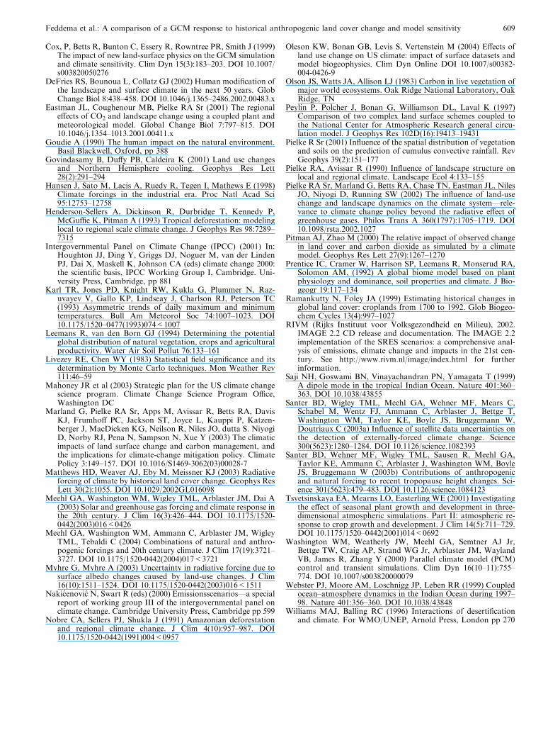
Cox, P, Betts R, Bunton C, Essery R, Rowntree PR, Smith J (1999)The impact of new land-surface physics on the GCM simulationand climate sensitivity. Clim Dyn 15(3):183–203. DOI 10.1007/s003820050276

DeFries RS, Bounoua L, Collatz GJ (2002) Human modification ofthe landscape and surface climate in the next 50 years. GlobChange Biol 8:438–458. DOI 10.1046/j.1365–2486.2002.00483.x

Eastman JL, Coughenour MB, Pielke RA Sr (2001) The regionaleffects of CO2 and landscape change using a coupled plant andmeteorological model. Global Change Biol 7:797–815. DOI10.1046/j.1354–1013.2001.00411.x

Goudie A (1990) The human impact on the natural environment.Basil Blackwell, Oxford, pp 388

Govindasamy B, Duffy PB, Caldeira K (2001) Land use changesand Northern Hemisphere cooling. Geophys Res Lett28(2):291–294

Hansen J, Sato M, Lacis A, Ruedy R, Tegen I, Mathews E (1998)Climate forcings in the industrial era. Proc Natl Acad Sci95:12753–12758

Henderson-Sellers A, Dickinson R, Durbridge T, Kennedy P,McGuffie K, Pitman A (1993) Tropical deforestation: modelinglocal to regional scale climate change. J Geophys Res 98:7289–7315

Intergovernmental Panel on Climate Change (IPCC) (2001) In:Houghton JJ, Ding Y, Griggs DJ, Noguer M, van der LindenPJ, Dai X, Maskell K, Johnson CA (eds) climate change 2000:the scientific basis, IPCC Working Group I, Cambridge. Uni-versity Press, Cambridge, pp 881

Karl TR, Jones PD, Knight RW, Kukla G, Plummer N, Raz-uvayev V, Gallo KP, Lindseay J, Charlson RJ, Peterson TC(1993) Asymmetric trends of daily maximum and minimumtemperatures. Bull Am Meteorol Soc 74:1007–1023. DOI10.1175/1520–0477(1993)074<1007

Leemans R, van den Born GJ (1994) Determining the potentialglobal distribution of natural vegetation, crops and agriculturalproductivity. Water Air Soil Pollut 76:133–161

Livezey RE, Chen WY (1983) Statistical field significance and itsdetermination by Monte Carlo techniques. Mon Weather Rev111:46–59

Mahoney JR et al (2003) Strategic plan for the US climate changescience program. Climate Change Science Program Office,Washington DC

Marland G, Pielke RA Sr, Apps M, Avissar R, Betts RA, DavisKJ, Frumhoff PC, Jackson ST, Joyce L, Kauppi P, Katzen-berger J, MacDicken KG, Neilson R, Niles JO, dutta S. NiyogiD, Norby RJ, Pena N, Sampson N, Xue Y (2003) The climaticimpacts of land surface change and carbon management, andthe implications for climate-change mitigation policy. ClimatePolicy 3:149–157. DOI 10.1016/S1469-3062(03)00028-7

Matthews HD, Weaver AJ, Eby M, Meissner KJ (2003) Radiativeforcing of climate by historical land cover change. Geophys ResLett 30(2):1055. DOI 10.1029/2002GL016098

Meehl GA, Washington WM, Wigley TML, Arblaster JM, Dai A(2003) Solar and greenhouse gas forcing and climate response inthe 20th century. J Clim 16(3):426–444. DOI 10.1175/1520-0442(2003)016<0426

Meehl GA, Washington WM, Ammann C, Arblaster JM, WigleyTML, Tebaldi C (2004) Combinations of natural and anthro-pogenic forcings and 20th century climate. J Clim 17(19):3721–3727. DOI 10.1175/1520-0442(2004)017<3721

Myhre G, Myhre A (2003) Uncertainty in radiative forcing due tosurface albedo changes caused by land-use changes. J Clim16(10):1511–1524. DOI 10.1175/1520-0442(2003)016<1511

Nakicenovic N, Swart R (eds) (2000) Emissionsscenarios—a specialreport of working group III of the intergovernmental panel onclimate change. Cambridge University Press, Cambridge pp 599

Nobre CA, Sellers PJ, Shukla J (1991) Amazonian deforestationand regional climate change. J Clim 4(10):957–987. DOI10.1175/1520-0442(1991)004<0957

Oleson KW, Bonan GB, Levis S, Vertenstein M (2004) Effects ofland use change on US climate: impact of surface datasets andmodel biogeophysics. Clim Dyn Online DOI 10.1007/s00382-004-0426-9

Olson JS, Watts JA, Allison LJ (1983) Carbon in live vegetation ofmajor world ecosystems. Oak Ridge National Laboratory, OakRidge, TN

Peylin P, Polcher J, Bonan G, Williamson DL, Laval K (1997)Comparison of two complex land surface schemes coupled tothe National Center for Atmospheric Research general circu-lation model. J Geophys Res 102D(16):19413–19431

Pielke R Sr (2001) Influence of the spatial distribution of vegetationand soils on the prediction of cumulus convective rainfall. RevGeophys 39(2):151–177

Pielke RA, Avissar R (1990) Influence of landscape structure onlocal and regional climate. Landscape Ecol 4:133–155

Pielke RA Sr, Marland G, Betts RA, Chase TN, Eastman JL, NilesJO, Niyogi D, Running SW (2002) The influence of land-usechange and landscape dynamics on the climate system—rele-vance to climate change policy beyond the radiative effect ofgreenhouse gases. Philos Trans A 360(1797):1705–1719. DOI10.1098/rsta.2002.1027

Pitman AJ, Zhao M (2000) The relative impact of observed changein land cover and carbon dioxide as simulated by a climatemodel. Geophys Res Lett 27(9):1267–1270

Prentice IC, Cramer W, Harrison SP, Leemans R, Monserud RA,Solomon AM, (1992) A global biome model based on plantphysiology and dominance, soil properties and climate. J Bio-geogr 19:117–134

Ramankutty N, Foley JA (1999) Estimating historical changes inglobal land cover: croplands from 1700 to 1992. Glob Biogeo-chem Cycles 13(4):997–1027

RIVM (Rijks Instituut voor Volksgezondheid en Milieu), 2002.IMAGE 2.2 CD release and documentation. The IMAGE 2.2implementation of the SRES scenarios: a comprehensive anal-ysis of emissions, climate change and impacts in the 21st cen-tury. See http://www.rivm.nl/image/index.html for furtherinformation.

Saji NH, Goswami BN, Vinayachandran PN, Yamagata T (1999)A dipole mode in the tropical Indian Ocean. Nature 401:360–363. DOI 10.1038/43855

Santer BD, Wigley TML, Meehl GA, Wehner MF, Mears C,Schabel M, Wentz FJ, Ammann C, Arblaster J, Bettge T,Washington WM, Taylor KE, Boyle JS, Bruggemann W,Doutriaux C (2003a) Influence of satellite data uncertainties onthe detection of externally-forced climate change. Science300(5623):1280–1284. DOI 10.1126/science.1082393

Santer BD, Wehner MF, Wigley TML, Sausen R, Meehl GA,Taylor KE, Ammann C, Arblaster J, Washington WM, BoyleJS, Bruggemann W (2003b) Contributions of anthropogenicand natural forcing to recent tropopause height changes. Sci-ence 301(5623):479–483. DOI 10.1126/science.1084123

Tsvetsinskaya EA, Mearns LO, Easterling WE (2001) Investigatingthe effect of seasonal plant growth and development in three-dimensional atmospheric simulations. Part II: atmospheric re-sponse to crop growth and development. J Clim 14(5):711–729.DOI 10.1175/1520–0442(2001)014<0692

Washington WM, Weatherly JW, Meehl GA, Semtner AJ Jr,Bettge TW, Craig AP, Strand WG Jr, Arblaster JM, WaylandVB, James R, Zhang Y (2000) Parallel climate model (PCM)control and transient simulations. Clim Dyn 16(10–11):755–774. DOI 10.1007/s003820000079

Webster PJ, Moore AM, Loschnigg JP, Leben RR (1999) Coupledocean–atmosphere dynamics in the Indian Ocean during 1997–98. Nature 401:356–360. DOI 10.1038/43848

Williams MAJ, Balling RC (1996) Interactions of desertificationand climate. For WMO/UNEP, Arnold Press, London pp 270

Feddema et al.: A comparison of a GCM response to historical anthropogenic land cover change and model sensitivity 609