A Comparison of 2D-3D Pose Estimation Methods Thomas Petersen Aalborg University 2008

Welcome message from author
This document is posted to help you gain knowledge. Please leave a comment to let me know what you think about it! Share it to your friends and learn new things together.
Transcript
A Comparison of 2D-3D PoseEstimation Methods
Thomas Petersen
Aalborg University 2008

Aalborg University - Institute for Media Technology
Computer vision and graphics
Lautrupvang 15, 2750 Ballerup, Denmark
Phone +45 9940 2480
469573.g.portal.aau.dk
www.aau.dk
Abstract
This thesis describes pose estimation as an increasingly used area in augmen-tation and tracking with many different solutions and methods that constantlyundergo optimization and each has drawbacks and benefits. But the aim isalways speed, accuracy or both when it comes to real applications. Pose esti-mation is used in many areas but primarily tracking and augmentation issues,where another large area of finding 2D-2D correspondences is crucial researcharea today. Software like ARToolKit [11] tracks a flat marker and is able todraw 3D objects on top of it for augmentation purposes. It is very fast, becausethe accuracy is not the largest issue when the eye has to judge if it looks realor augmented. But the speed must be high for the eye to see it as real as thebackground.
There is not really a common standard of how to compare methods for poseestimation and there is no standard method to compare with. In this thesisefford is made to get a fair comparison and there is included a simple veryknown method as comparator.
In total there is 4 methods tested, they calculate the perspective from known2D-3D correspondences from image to point cloud. All have different limitationssuch as minimum amount of 2D-3D correspondence pairs or sensitivity to noisethat makes it unpredictable in noisy conditions. The benefits and drawbacksare listed for each method for easy comparison. The 3 methods are nonlinearCPC, PosIt and PosIt for coplanar points, while DLT is a linear method that isused because it is easy to implement and good for comparison.
All tests are done on fictive data to allow some extreme cases and to haveground truth for accurate comparisons. In short the tests made are: Noise

ii
test, increased number of points, planarity issues, distance to object and initialguesses.
The findings were many and shows that the methods are working very differently.So when choosing a method, one has to consider the application of it, and whatdata is available to the method.
Preface
This thesis was made at Computer Vision and Graphics (CVG), at AalborgUniversity Copenhagen (AAU) in partial fulfillment of the requirements for ac-quiring the Master of Science in Engineering (M.Sc.Eng).
The thesis was carried out over a period of 4 month for the amount of 30 ECTSpoints, completing 1 full semester.
AAU, June 2008
Thomas Petersen

iv

Acknowledgements
This thesis has been made with help that I would like to thank for: First ofall my supervisor and teacher Daniel Grest for providing code and assistancealong with it, and also to help guide me in the right direction. I also like tothank family and friends for support throughout this period, and especially mybrother for proofreading my report.

vi

Contents
Abstract i
Preface iii
Acknowledgements v
1 Introduction 1
2 Related Work 5
3 Theory 7
3.1 Overview . . . . . . . . . . . . . . . . . . . . . . . . . . . . . . . 7
3.2 Notation . . . . . . . . . . . . . . . . . . . . . . . . . . . . . . . . 8
3.3 Pinhole Camera Model . . . . . . . . . . . . . . . . . . . . . . . . 8
3.4 Non-linear Least Squares . . . . . . . . . . . . . . . . . . . . . . . 9
3.4.1 Gauss-Newton . . . . . . . . . . . . . . . . . . . . . . . . 9
viii CONTENTS
3.4.2 Levenberg-Marquardt . . . . . . . . . . . . . . . . . . . . 10
3.5 Pose and rigid motion . . . . . . . . . . . . . . . . . . . . . . . . 10
3.6 PosIt . . . . . . . . . . . . . . . . . . . . . . . . . . . . . . . . . . 12
3.6.1 Scaled Orthographic Projection . . . . . . . . . . . . . . . 12
3.6.2 The PosIt coordinate system . . . . . . . . . . . . . . . . 13
3.6.3 The PosIt Algorithm . . . . . . . . . . . . . . . . . . . . . 14
3.7 PosIt for coplanar points . . . . . . . . . . . . . . . . . . . . . . . 16
3.7.1 Finding poses . . . . . . . . . . . . . . . . . . . . . . . . . 17
3.8 Projection matrix . . . . . . . . . . . . . . . . . . . . . . . . . . . 19
3.9 Direct Linear Transform(DLT) . . . . . . . . . . . . . . . . . . . 20
3.10 Boxplot . . . . . . . . . . . . . . . . . . . . . . . . . . . . . . . . 21
4 Experiments 23
4.1 Tests . . . . . . . . . . . . . . . . . . . . . . . . . . . . . . . . . . 23
4.1.1 Overall algorithm and test setup . . . . . . . . . . . . . . 24
4.1.2 General limitations for all algorithms . . . . . . . . . . . . 25
4.1.2.1 CPC requires . . . . . . . . . . . . . . . . . . . . 25
4.1.2.2 PosIt requires . . . . . . . . . . . . . . . . . . . 26
4.1.2.3 PosIt Planar requires . . . . . . . . . . . . . . . 26
4.1.2.4 DLT requires . . . . . . . . . . . . . . . . . . . . 26
4.1.3 Test 1: Increasing noise level . . . . . . . . . . . . . . . . 26
4.1.3.1 Maximum accuracy . . . . . . . . . . . . . . . . 30
4.1.4 Test 2: Increased number of points . . . . . . . . . . . . . 33

CONTENTS ix
4.1.5 Test 3: Points shape is morphed into planarity . . . . . . 40
4.1.6 Test 4: Camera is moved very close to the points . . . . . 46
4.1.7 Test 5: Testing the initial guess for CPC . . . . . . . . . . 50
4.1.8 Test 6: Different implementation of PosIt . . . . . . . . . 54
5 Conclusion 57
A The Test Program 59

x CONTENTS
Chapter 1
Introduction
This thesis is about various methods for pose estimation and tests to revealhow they react in common and uncommon situations. A pose is defined asthe position and orientation of the camera in relation to the 3D structure. Inorder to estimate a pose, a 2D image, a 3D object and some camera parametersare needed depends on the method. The 2D image should show the points ofthe 3D object, which is called 2D-3D correspondences. A minimum number ofcorrespondences are required for each method to run. Fischler and Bolles [?]have used the term ”Perspective n-Point problem” or ”PnP problem”, for thistype of problem with n feature points.
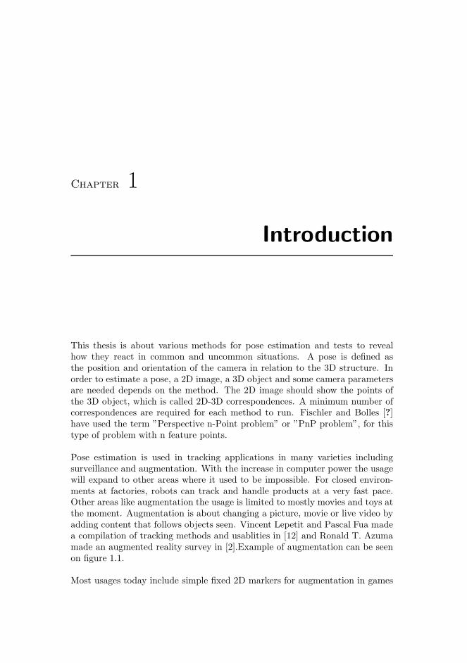
Pose estimation is used in tracking applications in many varieties includingsurveillance and augmentation. With the increase in computer power the usagewill expand to other areas where it used to be impossible. For closed environ-ments at factories, robots can track and handle products at a very fast pace.Other areas like augmentation the usage is limited to mostly movies and toys atthe moment. Augmentation is about changing a picture, movie or live video byadding content that follows objects seen. Vincent Lepetit and Pascal Fua madea compilation of tracking methods and usablities in [12] and Ronald T. Azumamade an augmented reality survey in [2].Example of augmentation can be seenon figure 1.1.
Most usages today include simple fixed 2D markers for augmentation in games
2 Introduction
Figure 1.1: Example of augmentation in Ogre.
for example Hitlab developed ARToolKit [11] and they made projects mainlyaround helping visual perception by 3D in areas like hospitals, learning andtreating phobias. Another company that makes virtual reality called Total Im-mersion uses marker tracking but also markerless tracking for movies, airplanecontrols, enhanced TV and much more. Common for companies like these is thattheir products aim for kids or learning aspects, but also the industry for moviesand presentations. All these areas seems to be focused on luxury but there isplans for more serious projects in health care with 3D bodies for operations forexample.
Some of the recent projects use structure from motion 1 to go from normalvacation images to build a 3D model of famous buildings. When a family isin vacation they should be able to take a picture of a building and the cameraknows what building and provides some info about the buildings history. Ituses GPS to narrow down the search of buildings and from maybe hundreds ofimages of one single building it can be pretty sure it guesses the right one.
Tracking people by their faces or body is also going to be the future on normalstreets to find criminals or track suspicious people. On the website Earthcam2
you can log in and see cameras from all over the world in famous places with highpopulation. This might just be the beginning of a surveillance era where we willbe watched in all public places. England has a very dense camera network in
1http://www.mip.informatik.uni-kiel.de/tiki-index.php?page=3D+reconstruction+from+images2http://www.earthcam.com/network/
3
London that is being tested with face recognition. It was proven to be useful atthe London bombing in 7th july 2005 where images of the terrorists was foundfrom several cameras around London. China uses face recognition to keep trackof hooligans that serves 1 year for making problems, and they can easy denythem access to soccer games. This all illustrates the importance of survaillanceand that it might be used for tracking other things than faces in just a matterof time.
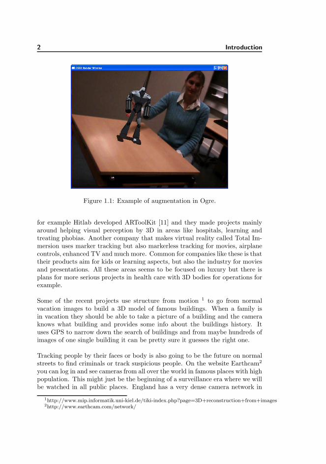
Several algorithms with the same goal have been tested against each other undervarious circumstances. The goal for all algorithms was to go from 2D-3D cor-respondences to a camera pose as seen on figure 1.2. The input for the systemis a known 3D structure made of points and these points have been related to2D points on an photo taken of the same 3D structure. This step of 2D-2Dmatching is not described here but is also a vast area of research today. For thepose to be defined both translation and rotation needs to be found, and in theresults here both are plotted, because the algorithms proved to not necessarilygive same accuracy for both.
Figure 1.2: Perspective projection illustrated for 4 points observed from camera.
The tested algorithms are CPC(CamPoseCalib) from [3], DLT [4], PosIt [6] anda planar version of PosIt [5]. There is no single place where all these have beencompared for speed and accuracy nor the special cases where 1 algorithm mightnot work properly. So this report is about special cases and common standardsof comparison between such algorithms.

4 Introduction
Chapter 2
Related Work
Many people have come up with innovative ideas for optimizing this processof finding a pose from 2D-3D correspondences. Ranging from simple ones likeDLT [4] to complex ones like PosIt [6]. Not only complexity vary a lot but alsothe approach can be either iteratively like [3] [6] [11] or non iterative like [4] or[8].
Most of the algorithms are based on a linear or nonlinear system of equationsthat needs to be solved, but how they get these equations and how many pa-rameters to be estimated is very different. All algorithms are not made for thesame purpose, still they all aim for speed and accuracy in their area. For ex-ample [8] is made to work well for many points since the system of equationshas the same computation time for higher amount of points. The idea is to use4 control points that are not coplanar, and they define all points according tothese control points so they only need to find the control points.
DLT [4] was first used in photogrametry and then later in computer vision. Itis the simplest method for finding the pose, by finding all the 12 parameters inthe projection matrix it will be slower than any other algorithm. Note that itis expected to be the weaker of the methods tested and included because it isoften used as a simple method that does not require initial guess and it is easyto implement.

6 Related Work
PosIt [6] is a method developed by Daniel DeMenthon in 1995 where it waspublished as a pose finder in 25 lines of code (mathematica). A fast method thatdoes not work with perspective projection as most other methods, but insteaduses orthographic projection that is simpler to work with and can approximateperspective to find the correct pose.
Coplanar PosIt [5] was also made by DeMenthon because PosIt does not workwell for planar or close to planar point clouds. Another issue when dealing withplanar point clouds is that there is often 2 solutions that are very close, andwhile normal algorithms choose either one, this planar version returns both.This is needed in some cases when there is no prior knowledge and a decisionhas to be made which pose is the right one. With prior knowledge you can limitthe pose change from each frame in a video sequence so it does not guess theopposite pose.
CPC stands for CamPoseCalib and is the method from BIAS [10], which is animage library made in Kiel 2006. It is based on the Gauss-Newton methodand nonlinear least squares optimization, originally published in [3]. A flexiblemethod, because it has a lot of options that are not described here. Howeverthese additional methods (like outlier mitigation) are not used in the compar-ison. More about Gauss-Newton and this special implementation can can befound in chapter 3 of [9].
Chapter 3
Theory
3.1 Overview
The 4 different algorithms have very unique theoretical background and thisis useful for understanding the test outcome in chapter 4. This chapter willgive basic information on notation and coordinate system information beforeexplaining the tested methods.
1. Notation
2. Pinhole Camera Model
3. Non-linear Least Squares
4. Pose and rigid motion
5. Posit
6. PosIt for coplanar points
7. Projection matrix
8. Direct Linear Transform(DLT)
9. Boxplot
8 Theory
3.2 Notation
Because of all the algorithms have different origin they come with various nota-tion that is presented here with one common notation:
s, θ, x ∈ R a scalar valuem ∈ R
2 2D points from perspective projectionM ∈ R
3 3D pointsp′ ∈ R
2 2D point from SOP(scaled orthographic projection)A, R, P ∈ R
n×m matrix of size n × m
functions:m(θ, p) 3D motion function for point m and parameters θ
Algorithms:CPC Gauss Newtons method from BIAS [10].PosIt BIAS version of PosIt [6].DLT Direct linear transform from [4].
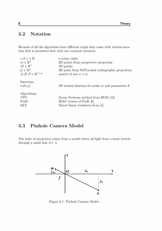
3.3 Pinhole Camera Model
The basic of projection comes from a model where all light from a scene travelsthrough a small hole 3.1. x
Figure 3.1: Pinhole Camera Model.
3.4 Non-linear Least Squares 9
Figure 3.1 shows simple pinhole princip where:
ym
f=
ya
xa
(3.1)
ym = −fya
xa
(3.2)
The 3D point a is projected through origin O to imageplane along ym withnormal in x direction to 2D image point m. The coordinate ym found in 3.2 isthe first coordinate of the 2D point in the image, the second can be found inthe same manner by looking from above(along y) and do the same calculations.
3.4 Non-linear Least Squares
The parameters describing a pose are estimated by minimizing an objectivefunction. The minimization is a non-linear least squares problem and is solvedwith Gauss-Newtons method. The objective function depends on the input weneed to estimate. A general non-linear least squares problem reads:
φ = argminφ
m∑
i=1
(ri(φ))2 (3.3)
This minimization is iterative and there are 2 stop criteria: when overall erroris lower than a threshold between image points observed and back projectedpoints from the 3D model. The threshold is called epsilon and in CPC it isdefined for both the rotational change and the 2D-2D change. The second stopvriteria is when a certain number of iterations is reached it stops.
3.4.1 Gauss-Newton
CPC from [10] is using the Gauss-Newton method to estimate the pose. Thismethod uses first order derivatives of the residual (for residual see equation 3.4).
ri(φ) (3.4)
Gauss-Newton approximates the hessian by leaving out the second order deriva-tives. The method called Newtons method uses also second order derivatives.
10 Theory
This method works analytically and not numerically, meaning it does not ”shake”the object to try and find derivatives, instead it already has the function for thederivative directly. A ”Shake” means a small change in parameters and thenchecking how that affected the error rate. The disadvantage about numericalapproach is the size of the ”shake” needs to be predefined and then does nothave to show the actual slope in the parameter space for a given situation.
For minimizing the objective function we need the Jacobian (first order deriva-tive of the residual functions) and from that update the parameters as seen inequation 3.5:
θt+1 = θt − (JT J)−1JT r(θt) (3.5)
Where J is the jacobian found according to [9].
3.4.2 Levenberg-Marquardt
This extension to the Gauss-Newton method interpolates between Gauss-Newtonand gradient descend. This addition makes Gauss-Newton more robust meaningit can start far off the correct minimum and still find it. But if the initial guessis good then it can actually be a slower way to find the correct pose. This workslike dampening the parameter change that happens each iteration to make surethat Gauss-Newton always descends in parameter space. More details aboutLevenberg-Marquardt in [4].
3.5 Pose and rigid motion
In order to describe an object in 3D space all we need is rotation and translation.Let aobj be a 3D point in an object we like to know the world coordinates of,and (α, β, λ) be the Euler rotations around the 3 world axis. Then the aw inworld coordinate system is given by:
aw = (θx, θy, θz)T + (Rex(α) ◦ Rey(β) ◦ Rez(λ))(aobj) (3.6)
Where (ex, ey, ez) denotes the world coordinate system and the whole thing isbuild on a translation and a rotation part.
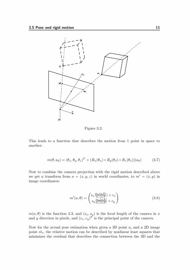
3.5 Pose and rigid motion 11
Figure 3.2:
This leads to a function that describes the motion from 1 point in space toanother:
m(θ, a0) = (θx, θy, θz)T + (Rx(θα) ◦ Ry(θβ) ◦ Rz(θλ))(a0) (3.7)
Now to combine the camera projection with the rigid motion described abovewe get a transform from a = (x, y, z) in world coordinates, to m′ = (x, y) inimage coordinates:
m′(a, θ) =
(
sxmx(a,θ)mz(a,θ
) + cx
symy(a,θ)mz(a,θ) + cy
)
(3.8)
m(a, θ) is the function 2.3, and (sx, sy) is the focal length of the camera in xand y direction in pixels, and (cx, cy)T is the principal point of the camera.
Now for the actual pose estimation when given a 3D point ai and a 2D imagepoint mi, the relative motion can be described by nonlinear least squares thatminimizes the residual that describes the connection between the 3D and the
12 Theory
2D (ai, mi).
d = ri(θ) = (m′(ai, θ) − mi) (3.9)
Where d is the 2D distance between 2 poses given a change in parameters θ.This is used for all iterations in CPC to find the next proper pose.
3.6 PosIt
This method is published by Daniel F. DeMenthon and Larry S. Davis in May1995. PosIt can find the pose of an object from a single image and does notrequire an initial guess. It requires 4 or more point correspondences between 3Dand 2D in order to find the pose of the object. The method is split in 2 where thefirst part is POS (Pose from Orthography and Scaling) that approximates theperspective projection with scaled orthographic projection and finds the rotationmatrix and translation vector from a linear set of equations. The second part isPOSIT which iteratively uses a scale factor for each point to enhance the foundorthographic projection and then uses POS on the new points instead of theoriginal ones until a threshold is met, either the number of iterations or the 2Dpixel difference averaged over all 2D correspondences.
3.6.1 Scaled Orthographic Projection
Scaled Orthographic Projection (SOP) is an approximation to perspective pro-jection because it assumes that all the points ai with (Xi, Yi, Zi) in cameracoordinate system, have Zi that is close to each other and can be set to thesame Z0 as taken from the reference point a0 on figure 3.3. In SOP, the im-age of a point ai of an object is a point p′i of the image plane G which hascoordinates:
x′
i = fXi
Z0, y′
i = fYi
Z0(3.10)
While in perspective projection instead of p′i we get mi:
xi = fXi
Zi
, yi = fYi
Zi
(3.11)
3.6 PosIt 13
The ratio called s = f/Z0 is the scaling factor of the SOP. Note that the refer-ence point a0 is the same in perspective and orthographic projection (x0, y0) =(x′
0, y′
0) = (0, 0).
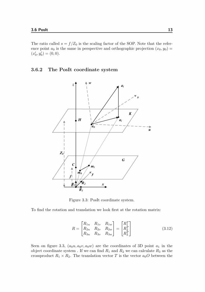
3.6.2 The PosIt coordinate system
Figure 3.3: PosIt coordinate system.
To find the rotation and translation we look first at the rotation matrix:
R =
R1u R1v R1w
R2u R2v R2w
R3u R3v R3w
=
RT1
RT2
RT3
(3.12)
Seen on figure 3.3, (a0u, a0v, a0w) are the coordinates of 3D point a1 in theobject coordinate system . If we can find R1 and R2 we can calculate R3 as thecrossproduct R1 × R2. The translation vector T is the vector a0O between the
14 Theory
center of projection O and origin of object coordinate system a0. a0 should bevisible image point m0 and T is then aligned with Om0 equal to Z0
fOm0. So
the pose defined by translation and rotation is found when we know R1, R2 andZ0.
3.6.3 The PosIt Algorithm
Starting with basic perspective projection that consist of a rotation matrix whereRT
1 , RT2 , RT
3 is the rows vectors of the matrix and a translation vector that isbetween the origin O center of the camera and a0 which is 0, 0, 0 in objectcoordinates. To project an object point a into image point m:
wxwyw
=
fRT1 fTx
fRT2 fTy
RT3 Tz
[
a1
]
(3.13)
The coordinates of the image point are homogenous and not affected by mul-tiplying with constants. All the elements in the perspective projection matrixare then multiplied with 1/Tz. Also the scaling factor s = f/Tz, that relatesthe distance to the object with the view of the camera.
[
wxwy
]
=
[
sRT1 sTx
sRT2 sTy
] [
a1
]
(3.14)
But now the w is instead:
w = R3· a/Tz + 1 (3.15)
In order for w to become 1 we need Tz to become much larger than R3· a,and then the projection would be the same for perspective projection. The dotproduct R3· a describes the projection of object point a unto the optical axisof the camera. Where R3 is the unit vector of the optical axis. When thedepth range of the object is small compared to the distance from the objectto the camera the perspective projection becomes the same as orthographicprojection.
[
xy
]
=
[
sRT1 sTx
sRT2 sTy
] [
a1
]
(3.16)
3.6 PosIt 15
The case of s = 1 is pure orthographic projection. The value s being differentfrom 1 can make up the difference to perspective projection. For each 2D pointPosIt estimates this scaling.
Now the general perspective equation can be rewritten as:
[
X Y Z 1]
[
sR1 sR2
sTx sTy
]
=[
wx wy]
(3.17)
Now when the iterations start we set initial w = 1 and then the only unknownsare sR1, sR2 and sTx, sTy that can be found with a system of 2 linear equationsassuming the rank of the matrix A is a least 4. So at least 4 points from allobject points have to be non-coplanar.
XsR(1, 1) + Y sR(1, 2) + ZsR(1, 3) + sTx = wx (3.18a)
XsR(2, 1) + Y sR(2, 2) + ZsR(2, 3) + sTx = wy (3.18b)
Where R(1, 1) means the first row and first column in the rotation matrix R.
I =[
sR1
]
(3.19)
J =[
sR2
]
(3.20)
So I and J are the scaled rows of the rotation matrix. To make a system ofequations we define K as the matrix we want to find, b as the 2D points and Aas the 3D points:
K =
[
IT sTx
JT sTy
]
(3.21)
A =
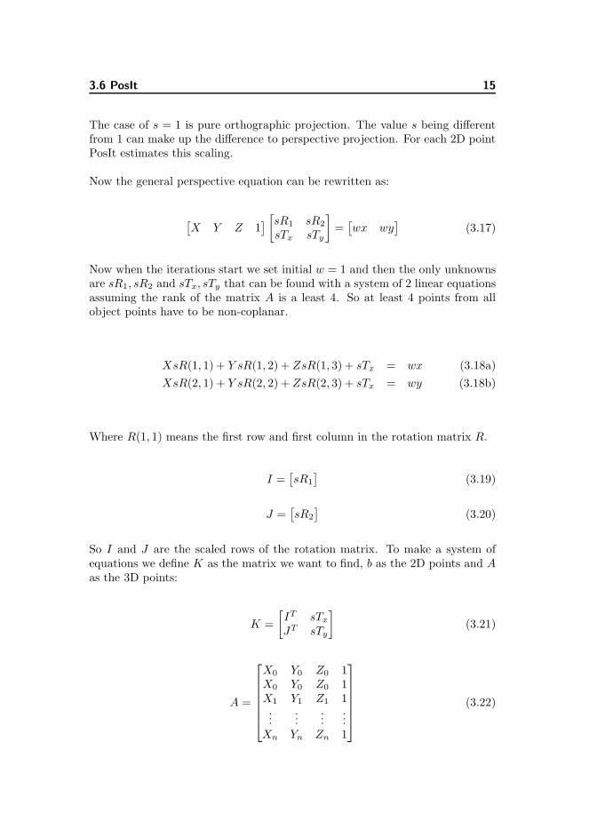
X0 Y0 Z0 1X0 Y0 Z0 1X1 Y1 Z1 1...
......
...Xn Yn Zn 1
(3.22)
16 Theory
b =
x0
y0
x1
y1
...xn
yn
(3.23)
The problem then simplifies to 3.24:
AK = b (3.24)
This can be solved as system of equations with least squares method. If n islarger than 4 it is overdetermined:
K = (AT A)−1AT b (3.25)
After finding I and J we can extract s and R1, R2 by the condition that theymust be unit vectors, and R3 as the crossproduct between R1 and R2. Tx andTy is found by deviding sTx, sTy with s.
As the iterations continue w from 3.18 for each point, becomes increasinglyaccurate until a stabil result is found or max number of iterations is reached.The scale factor w is updated according to 3.15.
3.7 PosIt for coplanar points
When dealing with planes there rises doubt about the pose because several posesthat are very different have the same orthographic projection 3.4. This planarversion of PosIt is finding all the poses and then choosing the best match. Morespecific it finds 2 poses for each iteration and either picks one or continue withboth options. This might look like a tree with n iterations and 2n solutions butonly 2 poses are kept at any time.
If the rank of A 3.22 is 3 instead of the 4 as required for regular PosIt, then wehave points distributed on a plane. Checking if the points are coplanar can bedone by calculating the rank with SVD (Singular Value Decomposition).
3.7 PosIt for coplanar points 17
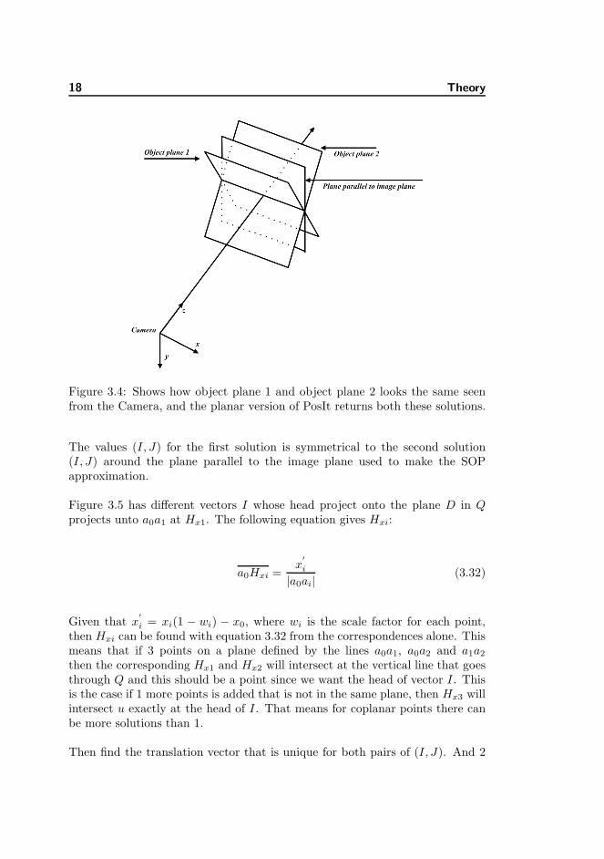
3.7.1 Finding poses
On figure 3.4 is illustrated the case where the object plane can have 2 verydifferent positions that returns the same 2D image correspondences. This isobject plane 1 and object plane 2 that both can be result of PosIt when dealingwith planarity. Given equation 3.19 and 3.20 if we could find 2 solution for bothI and J that would create 2 poses.
I = I0 + λu (3.26)
Where u is the unit vector normal to D figure 3.4 and λ is the coordinate of thehead of I along u. Same thing for J , µ is the coordinate of the head of J alongu:
J = J0 + µu (3.27)
The unknowns are λ, µ and u. u can be found because it is the normal to theobject plane D thus we know that a0ai. u = 0. u will then be the unit vectorof the null space of the matrix A. SVD and this knowledge can give you u andthen we only need λ and µ. To find them 2 more constrains are needed:
λµ = −I0. J0 (3.28)
Equation 3.28 means I and J are perpendicular. And 3.29 means I and J havethe same length:
λ2 − µ2 = I20 − J2
0 (3.29)
Equation 3.28 and 3.29 Now we have 2 equations with 2 unknowns and becausethis can be solved using a complex version and it gives 2 different solutions forboth I and J (see more in [7]).
I = I0 + ρcos(θ)u, J = J0 + ρsin(θ)u (3.30)
I = I0 − ρcos(θ)u, J = J0 − ρsin(θ)u (3.31)
The 2 solutions can be illustrated in the following manner:
18 Theory
Figure 3.4: Shows how object plane 1 and object plane 2 looks the same seenfrom the Camera, and the planar version of PosIt returns both these solutions.
The values (I, J) for the first solution is symmetrical to the second solution(I, J) around the plane parallel to the image plane used to make the SOPapproximation.
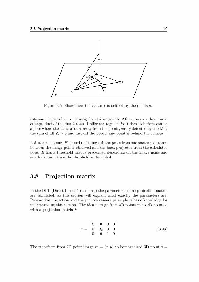
Figure 3.5 has different vectors I whose head project onto the plane D in Qprojects unto a0a1 at Hx1. The following equation gives Hxi:
a0Hxi =x
′
i
|a0ai|(3.32)
Given that x′
i = xi(1 − wi) − x0, where wi is the scale factor for each point,then Hxi can be found with equation 3.32 from the correspondences alone. Thismeans that if 3 points on a plane defined by the lines a0a1, a0a2 and a1a2
then the corresponding Hx1 and Hx2 will intersect at the vertical line that goesthrough Q and this should be a point since we want the head of vector I. Thisis the case if 1 more points is added that is not in the same plane, then Hx3 willintersect u exactly at the head of I. That means for coplanar points there canbe more solutions than 1.
Then find the translation vector that is unique for both pairs of (I, J). And 2
3.8 Projection matrix 19
Figure 3.5: Shows how the vector I is defined by the points ai.
rotation matrices by normalizing I and J we got the 2 first rows and last row iscrossproduct of the first 2 rows. Unlike the regular PosIt these solutions can bea pose where the camera looks away from the points, easily detected by checkingthe sign of all Zi > 0 and discard the pose if any point is behind the camera.
A distance measure E is used to distinguish the poses from one another, distancebetween the image points observed and the back projected from the calculatedpose. E has a threshold that is predefined depending on the image noise andanything lower than the threshold is discarded.
3.8 Projection matrix
In the DLT (Direct Linear Transform) the parameters of the projection matrixare estimated, so this section will explain what exactly the parameters are.Perspective projection and the pinhole camera principle is basic knowledge forunderstanding this section. The idea is to go from 3D points m to 2D points awith a projection matrix P :
P =
fx 0 0 00 fy 0 00 0 1 0
(3.33)
The transform from 2D point image m = (x, y) to homogenized 3D point a =
20 Theory
(x, y, z, 1)T , m = Pa then looks like:
mx
my
z
=
fx 0 0 00 fy 0 00 0 1 0
ax
ay
az
1
(3.34)
Where z is a scale factor that is used to normalize the 2D point m by mx
zand
my
z. The value of fx and fy is the focal length of the camera in x and y direc-
tion respectively. The rest of the projection matrix is rotation and translationparameters and the whole matrix is defined up to scale so it can be multipliedwith a constant and remains the same. For more information on calibration andfinding these parameters see [13].
3.9 Direct Linear Transform(DLT)
Direct Linear Transform (DLT) is the simple algorithm compared to CPC andPosIt.
DLT is around 10 times slower than 1 iteration of CPC because it estimates 11parameters and CPC only 6. After finding the 11 parameters the last one canbe found because the projection matrix P is defined up to scale. This methodis the simplest of the tested methods. It linearly estimates all 12 parametersin the projection matrix and need at least 6 points to do so. The projectionmatrix P can be described by vectors as follows:
P = (qT1 , q14, q
T2 , q24, q
T3 , q34) (3.35)
The 2D image coordinates and 3D object coordinates:
(ai, mi) = ((ai1, ai2, ai3)T , (ui, vi)
T ) (3.36)
From mi = Pai follows:
qT1 ai − uiq
T3 ai + q14 − uiq34 = 0 (3.37a)
qT2 ai − viq
T3 ai + q24 − viq34 = 0 (3.37b)
3.10 Boxplot 21
Because P is defined up to scale we can set the last q in P to 1 and thus:
A =
a11 a12 a13 1 0 0 0 0 −u1a11 −u1a12 −u1a13 −u1
0 0 0 0 a11 a12 a13 1 −v1a11 −v1a12 −v1a13 −v1
......
......
......
......
......
......
an1 an2 an3 1 0 0 0 0 −unan1 −unan2 −unan3 −un
0 0 0 0 an1 an2 an3 1 −vnan1 −vnan2 −vnan3 −vn
(3.38)
Now we can say Aq = 0. To find the q we need to have enough points n in an
and in this case 6 for 12 parameters and more will be over determined. Thenfind q with SVD as the smallest eigenvalue under the assumption that |q| = 1.See [1] for details.
3.10 Boxplot
This plot type is also known as box and whisker plot, it shows median, quar-tiles and whiskers/outliers. The boxplot was invented in 1977 by the Americanstatistician John Tukey. Quartile 1 (Q1) is the number which 25% of the datais lower than, and quartile 3 (Q3) is the number which 25% of the data is higherthan and Q2 is the median value. Now the interquartile range (IQR) is Q3-Q1and is used to decide which data points are marked as outliers. The standardvalue for this is 1.5IQR lower than Q1 or 1.5IQR higher than Q3.
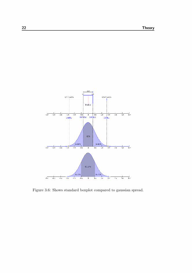
On figure 3.6 from 1 you see 3 axes, the 1st one is boxplot of a standard normaldistribution, 2nd shows how much of the data the different parts of the box-plot contains and the 3rd axes shows how the standard normal distribution ispresented using variance as comparison to the boxplot method. Note that nooutliers are shown here but later on they will be red X ’s.
1www.wikipedia.org
22 Theory
Figure 3.6: Shows standard boxplot compared to gaussian spread.
Chapter 4
Experiments
4.1 Tests
Here is a short description of each test and why it is relevant for testing followedby the actual test. Several angles are approached under each of these sectionsto find out what happens to accuracy and time in some extreme cases.
1. Overall algorithm and test setup
2. General limitations for all algorithms
3. Test 1: Increasing noise level
4. Test 2: Increased number of points
5. Test 3: Points shape is morphed into planarity
6. Test 4: Camera is moved very close to the points
7. Test 5: Testing the initial guess for CPC
8. Test 6: Different implementation of PosIt
24 Experiments
4.1.1 Overall algorithm and test setup
These tests were conducted on synthetic data points with values uniformly dis-tributed between −5 and +5 on x, y and z axis. One of these points will alwaysbe 0, 0, 0 in 3D space because the PosIt implementation requires this. All thepoints are projected with a virtual camera position to make the ground truthand gaussian noise is added to the 2D points to resemble real image noise. Thenoise has mean 0 and variance 0.2 as a standard value unless otherwise writtenin the specific test.
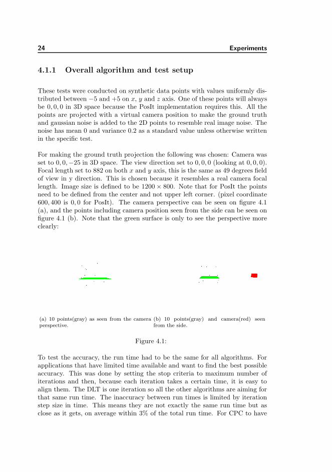
For making the ground truth projection the following was chosen: Camera wasset to 0, 0,−25 in 3D space. The view direction set to 0, 0, 0 (looking at 0, 0, 0).Focal length set to 882 on both x and y axis, this is the same as 49 degrees fieldof view in y direction. This is chosen because it resembles a real camera focallength. Image size is defined to be 1200 × 800. Note that for PosIt the pointsneed to be defined from the center and not upper left corner. (pixel coordinate600, 400 is 0, 0 for PosIt). The camera perspective can be seen on figure 4.1(a), and the points including camera position seen from the side can be seen onfigure 4.1 (b). Note that the green surface is only to see the perspective moreclearly:
(a) 10 points(gray) as seen from the cameraperspective.
(b) 10 points(gray) and camera(red) seenfrom the side.
Figure 4.1:
To test the accuracy, the run time had to be the same for all algorithms. Forapplications that have limited time available and want to find the best possibleaccuracy. This was done by setting the stop criteria to maximum number ofiterations and then, because each iteration takes a certain time, it is easy toalign them. The DLT is one iteration so all the other algorithms are aiming forthat same run time. The inaccuracy between run times is limited by iterationstep size in time. This means they are not exactly the same run time but asclose as it gets, on average within 3% of the total run time. For CPC to have

4.1 Tests 25
same run time as PosIt, CPC is run with 9 iterations and PosIt 400. This showsthat PosIt has less to calculate during one iteration than CPC. Also note thatCPC is provided the correct pose estimate at the first run of the test and afterthat uses the previous guess, unless otherwise noted in the test description.
PLOTS: 2 types of plots are used for showing the results, one is boxplot asdescribed in section 3.9, and second is using mean and standard deviation asarea plot. The reason for using standard deviation instead of variance is morerobustness when it comes to scaling and it is easier to interpret. AXES: Thetranslational error is the Euclidean distance between the perfect translation andthe guessed translation. Result is divided by the distance from the camera tothe world center. A translation error of 1 is then relative to a guessed cam-era position of 0,0,0 where the correct would be 0,0,-25. The rotational erroris the Euclidean distance between 2 Quaternion. All time measuring is donein nanoseconds and include only the computation of the result and not theconversions and initializations.
All the tests are done 100 times.
The descriptions below use above numbers unless otherwise noted.
4.1.2 General limitations for all algorithms
In order to work properly all the algorithms have some basic demands for theinput. This concerns the points but also the parameters required to find poses.
4.1.2.1 CPC requires
1. Initial guess of pose including projection matrix with focal lengths, skew,image size and center. The implementation also has a function to find agood initial pose, however this has not been used.
2. 3 or more 2D-3D correspondences.
3. 2D Points are defined from (0, 0) up to the size of the image or (1200, 800)in this thesis (origin top left).
4. Iteration number and limit on parameter change for rotational and trans-lation error.
26 Experiments
4.1.2.2 PosIt requires
1. Focal length, which is assumed to be same for x and y.
2. 4 or more non-coplanar 2D-3D correspondences.
3. 1st point must be (0, 0, 0)T in 3D and (0, 0)T in 2D.
4. 2D points are defined from the center of the image as (0, 0) (Origin atimage center).
5. Iteration number and pose accuracy.
6. Stop criteria either iterations or pose accuracy.
4.1.2.3 PosIt Planar requires
Same as PosIt. But for proper result the 3D points sould be perfectly coplanarsee Test 3.
4.1.2.4 DLT requires
1. 2D Points are defined from (0, 0) up to the size of the image or (1200, 800)in this thesis (Origin at top left).
4.1.3 Test 1: Increasing noise level
The noise level on the 2D points are increased variance from 0.0 to 10.0 (about3.3 pixels) with 100 steps of size 0.1 on an image of 1200×800 and no possibilityof points being outside the image. A total of 10 points was used.
10.0 noise level means noise with the variance of 10.0 is added to the 2D backprojected ground truth, to get the 2D points passed to the methods. Consideringa gaussian distribution the noise could be more than 10 pixels, but with a verylittle likelihood.
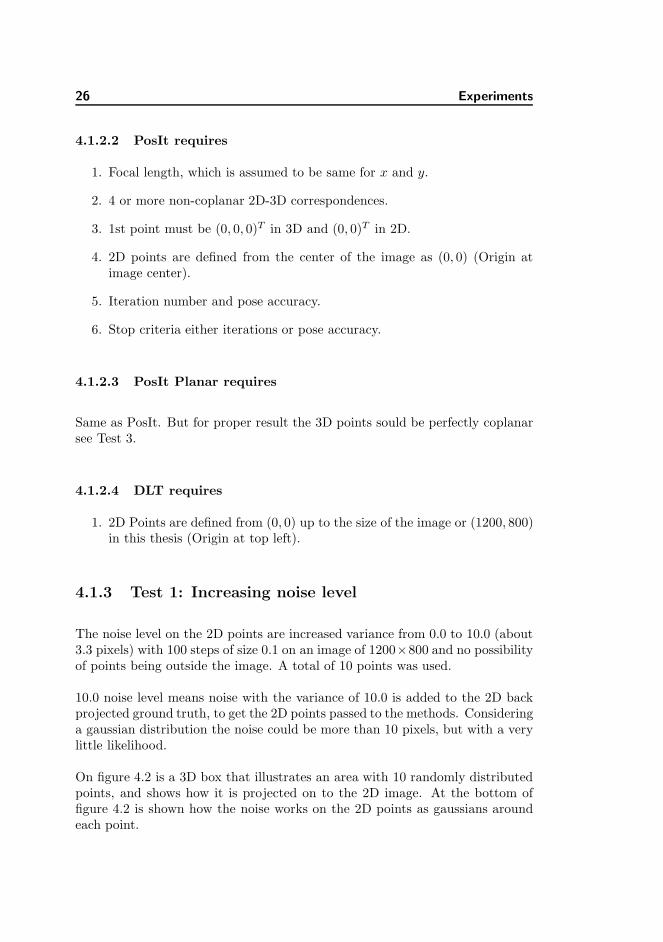
On figure 4.2 is a 3D box that illustrates an area with 10 randomly distributedpoints, and shows how it is projected on to the 2D image. At the bottom offigure 4.2 is shown how the noise works on the 2D points as gaussians aroundeach point.
4.1 Tests 27
Figure 4.2: Test 1 illustrated
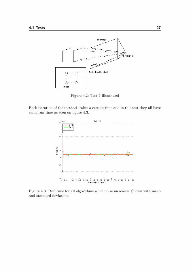
Each iteration of the methods takes a certain time and in this test they all havesame run time as seen on figure 4.3.
Figure 4.3: Run time for all algorithms when noise increases. Shown with meanand standard deviation.
28 Experiments
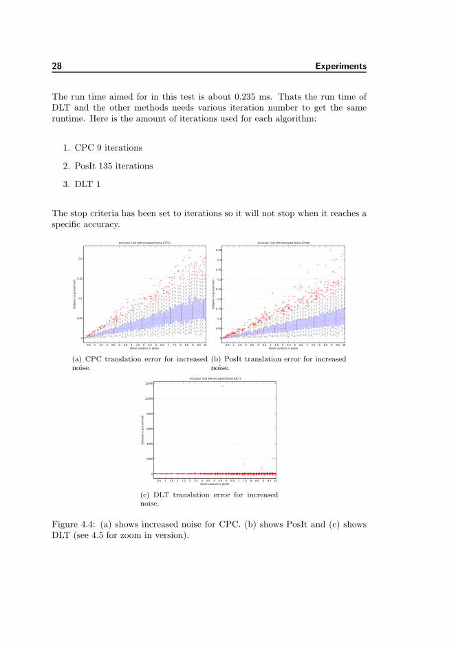
The run time aimed for in this test is about 0.235 ms. Thats the run time ofDLT and the other methods needs various iteration number to get the sameruntime. Here is the amount of iterations used for each algorithm:
1. CPC 9 iterations
2. PosIt 135 iterations
3. DLT 1
The stop criteria has been set to iterations so it will not stop when it reaches aspecific accuracy.
0.5 1 1.5 2 2.5 3 3.5 4 4.5 5 5.5 6 6.5 7 7.5 8 8.5 9 9.5 10
0
0.05
0.1
0.15
0.2
Dis
tanc
e to
gro
und
trut
h
Noise variance in pixels
Accuracy Test with increased Noise (CPC)
(a) CPC translation error for increasednoise.
0.5 1 1.5 2 2.5 3 3.5 4 4.5 5 5.5 6 6.5 7 7.5 8 8.5 9 9.5 10
0
0.05
0.1
0.15
0.2
0.25
0.3
0.35
0.4
0.45
Dis
tanc
e to
gro
und
trut
h
Noise variance in pixels
Accuracy Test with increased Noise (PosIt)
(b) PosIt translation error for increasednoise.
0.5 1 1.5 2 2.5 3 3.5 4 4.5 5 5.5 6 6.5 7 7.5 8 8.5 9 9.5 10
0
2000
4000
6000
8000
10000
12000
Dis
tanc
e to
gro
und
trut
h
Noise variance in pixels
Accuracy Test with increased Noise (DLT)
(c) DLT translation error for increasednoise.
Figure 4.4: (a) shows increased noise for CPC. (b) shows PosIt and (c) showsDLT (see 4.5 for zoom in version).
4.1 Tests 29
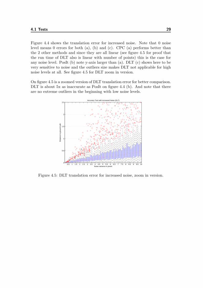
Figure 4.4 shows the translation error for increased noise. Note that 0 noiselevel means 0 errors for both (a), (b) and (c). CPC (a) performs better thanthe 2 other methods and since they are all linear (see figure 4.5 for proof thatthe run time of DLT also is linear with number of points) this is the case forany noise level. PosIt (b) note y-axis larger than (a). DLT (c) shows here to bevery sensitive to noise and the outliers size makes DLT not applicable for highnoise levels at all. See figure 4.5 for DLT zoom in version.
On figure 4.5 is a zoomed version of DLT translation error for better comparison.DLT is about 5x as inaccurate as PosIt on figure 4.4 (b). And note that thereare no extreme outliers in the beginning with low noise levels.
0.5 1 1.5 2 2.5 3 3.5 4 4.5 5 5.5 6 6.5 7 7.5 8 8.5 9 9.5 100
0.5
1
1.5
2
2.5
Dis
tanc
e to
gro
und
trut
h
Noise variance in pixels
Accuracy Test with increased Noise (DLT)
Figure 4.5: DLT translation error for increased noise, zoom in version.
30 Experiments
0.5 1 1.5 2 2.5 3 3.5 4 4.5 5 5.5 6 6.5 7 7.5 8 8.5 9 9.5 10
0
0.01
0.02
0.03
0.04
0.05
0.06
0.07
0.08
Dis
tanc
e to
gro
und
trut
h(ro
t)
Noise variance in pixels
Accuracy Test with increased Noise (CPC)
(a) CPC rotational error for increasednoise.
0.5 1 1.5 2 2.5 3 3.5 4 4.5 5 5.5 6 6.5 7 7.5 8 8.5 9 9.5 10
0
0.02
0.04
0.06
0.08
0.1
0.12
0.14
0.16
Dis
tanc
e to
gro
und
trut
h(ro
t)
Noise variance in pixels
Accuracy Test with increased Noise (posit)
(b) PosIt rotational error for increasednoise.
0.5 1 1.5 2 2.5 3 3.5 4 4.5 5 5.5 6 6.5 7 7.5 8 8.5 9 9.5 10
0
0.2
0.4
0.6
0.8
1
1.2
1.4
Dis
tanc
e to
gro
und
trut
h(ro
t)
Noise variance in pixels
Accuracy Test with increased Noise (DLT)
(c) DLT rotational error for increasednoise.
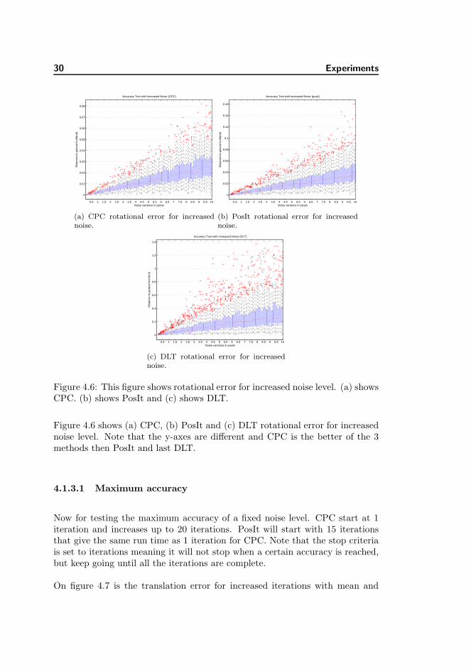
Figure 4.6: This figure shows rotational error for increased noise level. (a) showsCPC. (b) shows PosIt and (c) shows DLT.
Figure 4.6 shows (a) CPC, (b) PosIt and (c) DLT rotational error for increasednoise level. Note that the y-axes are different and CPC is the better of the 3methods then PosIt and last DLT.
4.1.3.1 Maximum accuracy
Now for testing the maximum accuracy of a fixed noise level. CPC start at 1iteration and increases up to 20 iterations. PosIt will start with 15 iterationsthat give the same run time as 1 iteration for CPC. Note that the stop criteriais set to iterations meaning it will not stop when a certain accuracy is reached,but keep going until all the iterations are complete.
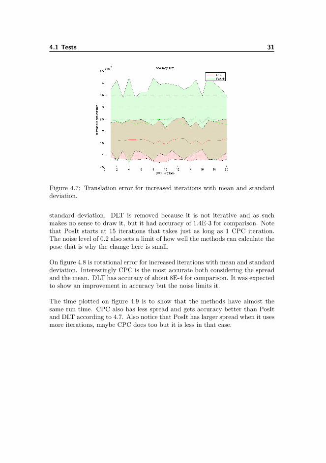
On figure 4.7 is the translation error for increased iterations with mean and
4.1 Tests 31
Figure 4.7: Translation error for increased iterations with mean and standarddeviation.
standard deviation. DLT is removed because it is not iterative and as suchmakes no sense to draw it, but it had accuracy of 1.4E-3 for comparison. Notethat PosIt starts at 15 iterations that takes just as long as 1 CPC iteration.The noise level of 0.2 also sets a limit of how well the methods can calculate thepose that is why the change here is small.
On figure 4.8 is rotational error for increased iterations with mean and standarddeviation. Interestingly CPC is the most accurate both considering the spreadand the mean. DLT has accuracy of about 8E-4 for comparison. It was expectedto show an improvement in accuracy but the noise limits it.
The time plotted on figure 4.9 is to show that the methods have almost thesame run time. CPC also has less spread and gets accuracy better than PosItand DLT according to 4.7. Also notice that PosIt has larger spread when it usesmore iterations, maybe CPC does too but it is less in that case.
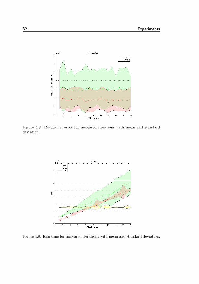
32 Experiments
Figure 4.8: Rotational error for increased iterations with mean and standarddeviation.
Figure 4.9: Run time for increased iterations with mean and standard deviation.
4.1 Tests 33
4.1.4 Test 2: Increased number of points
This test is made to find out what happens if we add more points to calculatethe output pose. The result is plotted from 3−6 (depends on the method) pointsup to 40 points and you can see the output is for a fixed number of iterations.
The CPC method has the correct projection matrix as initial guess, but becauseof the noise added the accuracy will not be perfect.
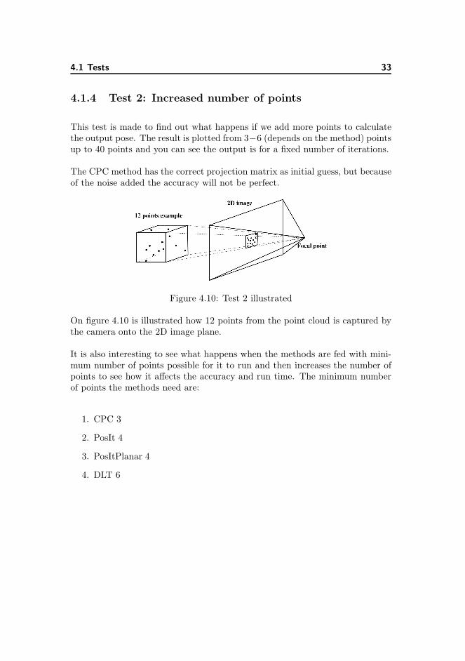
Figure 4.10: Test 2 illustrated
On figure 4.10 is illustrated how 12 points from the point cloud is captured bythe camera onto the 2D image plane.
It is also interesting to see what happens when the methods are fed with mini-mum number of points possible for it to run and then increases the number ofpoints to see how it affects the accuracy and run time. The minimum numberof points the methods need are:
1. CPC 3
2. PosIt 4
3. PosItPlanar 4
4. DLT 6
34 Experiments
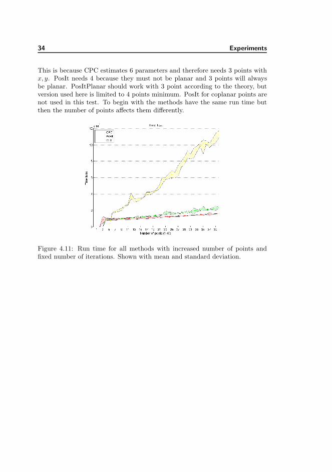
This is because CPC estimates 6 parameters and therefore needs 3 points withx, y. PosIt needs 4 because they must not be planar and 3 points will alwaysbe planar. PosItPlanar should work with 3 point according to the theory, butversion used here is limited to 4 points minimum. PosIt for coplanar points arenot used in this test. To begin with the methods have the same run time butthen the number of points affects them differently.
Figure 4.11: Run time for all methods with increased number of points andfixed number of iterations. Shown with mean and standard deviation.
4.1 Tests 35
On figure 4.11 is the run time of each algorithm as the number of points increasesto 40 with mean and standard deviation. DLT stands out as the worst methodand more than doubles in time when the number of points is doubled. So DLTis linearly increasing time for more points added. PosIt and CPC are close butCPC is the best at handling more points. CPC’s run time becomes 1.84 timesslower from 6-45 points. PosIt’s run time becomes 2.76 times slower from 6-45points. DLT’s run time becomes 7.92 times slower from 6-45 points.
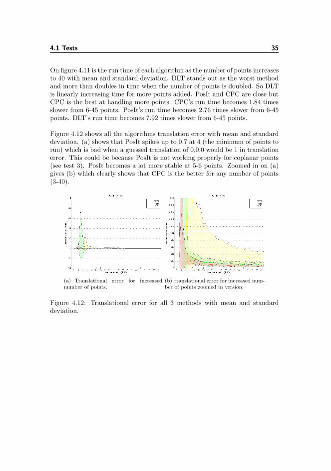
Figure 4.12 shows all the algorithms translation error with mean and standarddeviation. (a) shows that PosIt spikes up to 0.7 at 4 (the minimum of points torun) which is bad when a guessed translation of 0,0,0 would be 1 in translationerror. This could be because PosIt is not working properly for coplanar points(see test 3). PosIt becomes a lot more stable at 5-6 points. Zoomed in on (a)gives (b) which clearly shows that CPC is the better for any number of points(3-40).
(a) Translational error for increasednumber of points.
(b) translational error for increased num-ber of points zoomed in version.
Figure 4.12: Translational error for all 3 methods with mean and standarddeviation.
36 Experiments
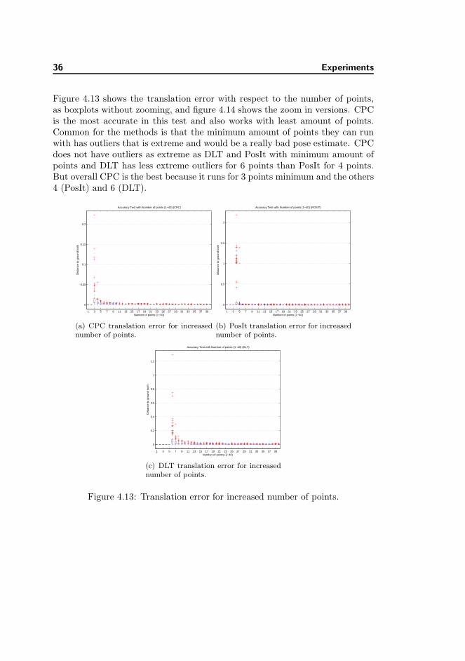
Figure 4.13 shows the translation error with respect to the number of points,as boxplots without zooming, and figure 4.14 shows the zoom in versions. CPCis the most accurate in this test and also works with least amount of points.Common for the methods is that the minimum amount of points they can runwith has outliers that is extreme and would be a really bad pose estimate. CPCdoes not have outliers as extreme as DLT and PosIt with minimum amount ofpoints and DLT has less extreme outliers for 6 points than PosIt for 4 points.But overall CPC is the best because it runs for 3 points minimum and the others4 (PosIt) and 6 (DLT).
1 3 5 7 9 11 13 15 17 19 21 23 25 27 29 31 33 35 37 39
0
0.05
0.1
0.15
0.2
Dis
tanc
e to
gro
und
trut
h
Number of points (1−40)
Accuracy Test with Number of points (1−40) (CPC)
(a) CPC translation error for increasednumber of points.
1 3 5 7 9 11 13 15 17 19 21 23 25 27 29 31 33 35 37 39
0
0.5
1
1.5
2
Dis
tanc
e to
gro
und
trut
h
Number of points (1−40)
Accuracy Test with Number of points (1−40) (POSIT)
(b) PosIt translation error for increasednumber of points.
1 3 5 7 9 11 13 15 17 19 21 23 25 27 29 31 33 35 37 39
0
0.2
0.4
0.6
0.8
1
1.2
Dis
tanc
e to
gro
und
trut
h
Number of points (1−40)
Accuracy Test with Number of points (1−40) (DLT)
(c) DLT translation error for increasednumber of points.
Figure 4.13: Translation error for increased number of points.
4.1 Tests 37
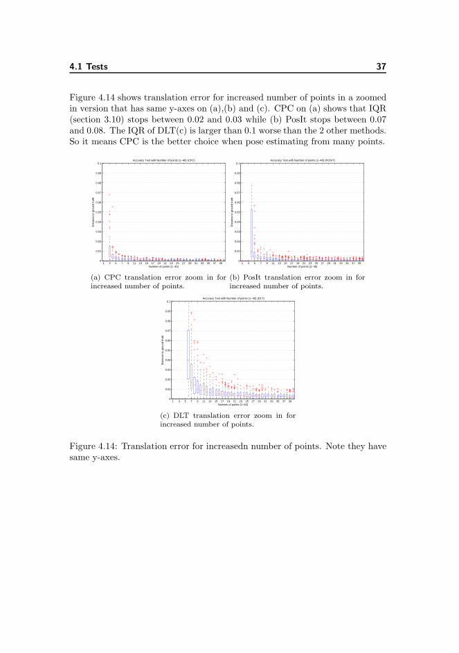
Figure 4.14 shows translation error for increased number of points in a zoomedin version that has same y-axes on (a),(b) and (c). CPC on (a) shows that IQR(section 3.10) stops between 0.02 and 0.03 while (b) PosIt stops between 0.07and 0.08. The IQR of DLT(c) is larger than 0.1 worse than the 2 other methods.So it means CPC is the better choice when pose estimating from many points.
1 3 5 7 9 11 13 15 17 19 21 23 25 27 29 31 33 35 37 390
0.01
0.02
0.03
0.04
0.05
0.06
0.07
0.08
0.09
0.1
Dis
tanc
e to
gro
und
trut
h
Number of points (1−40)
Accuracy Test with Number of points (1−40) (CPC)
(a) CPC translation error zoom in forincreased number of points.
1 3 5 7 9 11 13 15 17 19 21 23 25 27 29 31 33 35 37 390
0.01
0.02
0.03
0.04
0.05
0.06
0.07
0.08
0.09
0.1
Dis
tanc
e to
gro
und
trut
h
Number of points (1−40)
Accuracy Test with Number of points (1−40) (POSIT)
(b) PosIt translation error zoom in forincreased number of points.
1 3 5 7 9 11 13 15 17 19 21 23 25 27 29 31 33 35 37 390
0.01
0.02
0.03
0.04
0.05
0.06
0.07
0.08
0.09
0.1
Dis
tanc
e to
gro
und
trut
h
Number of points (1−40)
Accuracy Test with Number of points (1−40) (DLT)
(c) DLT translation error zoom in forincreased number of points.
Figure 4.14: Translation error for increasedn number of points. Note they havesame y-axes.
38 Experiments
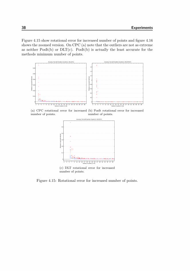
Figure 4.15 show rotational error for increased number of points and figure 4.16shows the zoomed version. On CPC (a) note that the outliers are not as extremeas neither PosIt(b) or DLT(c). PosIt(b) is actually the least accurate for themethods minimum number of points.
1 3 5 7 9 11 13 15 17 19 21 23 25 27 29 31 33 35 37 39
0
0.01
0.02
0.03
0.04
0.05
0.06
Dis
tanc
e to
gro
und
trut
h(ro
t)
Number of points (1−40)
Accuracy Test with Number of points (1−40) (CPC)
(a) CPC rotational error for increasednumber of points.
1 3 5 7 9 11 13 15 17 19 21 23 25 27 29 31 33 35 37 39
0
0.2
0.4
0.6
0.8
1
1.2
1.4
1.6
Dis
tanc
e to
gro
und
trut
h(ro
t)
Number of points (1−40)
Accuracy Test with Number of points (1−40) (POSIT)
(b) PosIt rotational error for increasednumber of points.
1 3 5 7 9 11 13 15 17 19 21 23 25 27 29 31 33 35 37 39
0
0.1
0.2
0.3
0.4
0.5
Dis
tanc
e to
gro
und
trut
h(ro
t)
Number of points (1−40)
Accuracy Test with Number of points (1−40) (DLT)
(c) DLT rotational error for increasednumber of points.
Figure 4.15: Rotational error for increased number of points.
4.1 Tests 39
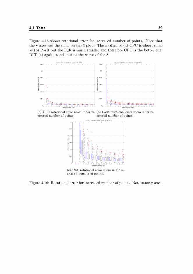
Figure 4.16 shows rotational error for increased number of points. Note thatthe y-axes are the same on the 3 plots. The median of (a) CPC is about sameas (b) PosIt but the IQR is much smaller and therefore CPC is the better one.DLT (c) again stands out as the worst of the 3.
1 3 5 7 9 11 13 15 17 19 21 23 25 27 29 31 33 35 37 390
0.005
0.01
0.015
0.02
0.025
0.03
Dis
tanc
e to
gro
und
trut
h(ro
t)
Number of points (1−40)
Accuracy Test with Number of points (1−40) (CPC)
(a) CPC rotational error zoom in for in-creased number of points.
1 3 5 7 9 11 13 15 17 19 21 23 25 27 29 31 33 35 37 390
0.005
0.01
0.015
0.02
0.025
0.03
Dis
tanc
e to
gro
und
trut
h(ro
t)
Number of points (1−40)
Accuracy Test with Number of points (1−40) (POSIT)
(b) PosIt rotational error zoom in for in-creased number of points.
1 3 5 7 9 11 13 15 17 19 21 23 25 27 29 31 33 35 37 390
0.005
0.01
0.015
0.02
0.025
0.03
Dis
tanc
e to
gro
und
trut
h(ro
t)
Number of points (1−40)
Accuracy Test with Number of points (1−40) (DLT)
(c) DLT rotational error zoom in for in-creased number of points.
Figure 4.16: Rotational error for increased number of points. Note same y-axes.
40 Experiments
4.1.5 Test 3: Points shape is morphed into planarity
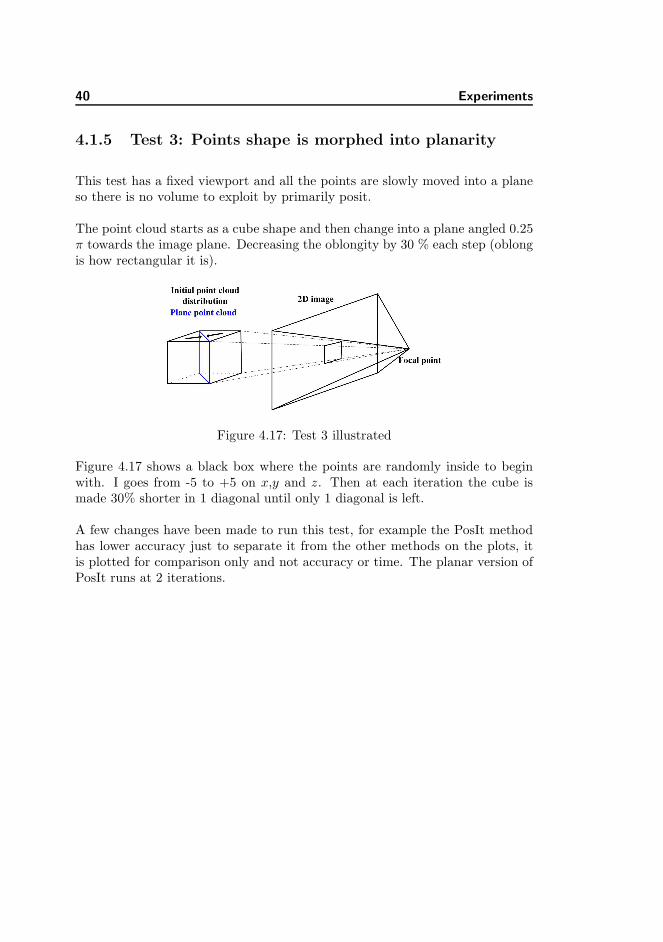
This test has a fixed viewport and all the points are slowly moved into a planeso there is no volume to exploit by primarily posit.
The point cloud starts as a cube shape and then change into a plane angled 0.25π towards the image plane. Decreasing the oblongity by 30 % each step (oblongis how rectangular it is).
Figure 4.17: Test 3 illustrated
Figure 4.17 shows a black box where the points are randomly inside to beginwith. I goes from -5 to +5 on x,y and z. Then at each iteration the cube ismade 30% shorter in 1 diagonal until only 1 diagonal is left.
A few changes have been made to run this test, for example the PosIt methodhas lower accuracy just to separate it from the other methods on the plots, itis plotted for comparison only and not accuracy or time. The planar version ofPosIt runs at 2 iterations.
4.1 Tests 41
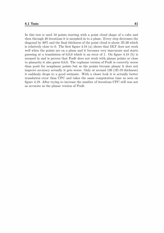
In this test is used 10 points starting with a point cloud shape of a cube andthen through 40 iterations it is morphed in to a plane. Every step decreases thediagonal by 30% and the final thickness of the point cloud is about 1E-30 whichis relatively close to 0. The first figure 4.18 (a) shows that DLT does not workwell when the points are on a plane and it becomes very inaccurate and startsguessing at a translation of 0,0,0 which is an error of 1. On figure 4.18 (b) iszoomed in and is proven that PosIt does not work with planar points or closeto planarity it also guess 0,0,0. The coplanar version of PosIt is correctly worsethan posit for nonplanar points but as the points become planar it does notimprove accuracy actually it gets worse. Only at around 130 (1E-19 thickness)it suddenly drops to a good estimate. With a closer look it is actually bettertranslation error than CPC and takes the same computation time as seen onfigure 4.19. After trying to increase the number of iterations CPC still was notas accurate as the planar version of PosIt.
42 Experiments
(a) All methods translation error, forpoints moved to planarity.
(b) All methods translation errorzoomed, for points moved to planarity.
(c) All methods translation error, forpoints moved to planarity zoomed evenmore to show CPC and posit planarwhen points are coplanar.
Figure 4.18: Translation error for all methods when point cloud is morphed intoplanarity. Shown with mean and standard deviation.
4.1 Tests 43
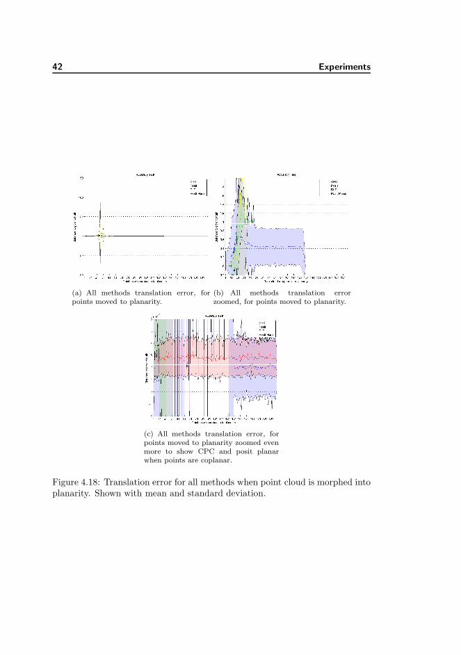
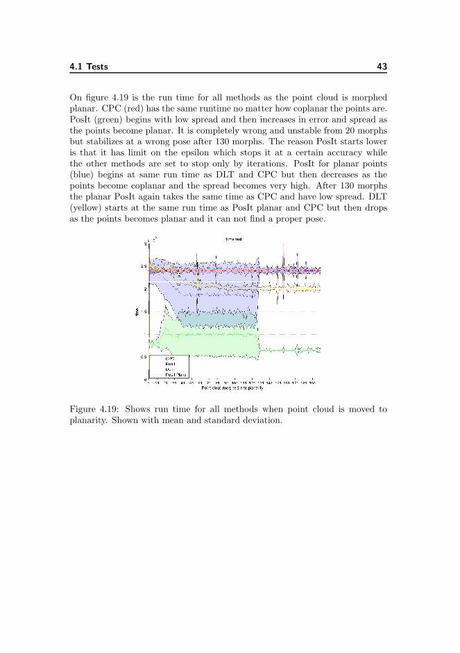
On figure 4.19 is the run time for all methods as the point cloud is morphedplanar. CPC (red) has the same runtime no matter how coplanar the points are.PosIt (green) begins with low spread and then increases in error and spread asthe points become planar. It is completely wrong and unstable from 20 morphsbut stabilizes at a wrong pose after 130 morphs. The reason PosIt starts loweris that it has limit on the epsilon which stops it at a certain accuracy whilethe other methods are set to stop only by iterations. PosIt for planar points(blue) begins at same run time as DLT and CPC but then decreases as thepoints become coplanar and the spread becomes very high. After 130 morphsthe planar PosIt again takes the same time as CPC and have low spread. DLT(yellow) starts at the same run time as PosIt planar and CPC but then dropsas the points becomes planar and it can not find a proper pose.
Figure 4.19: Shows run time for all methods when point cloud is moved toplanarity. Shown with mean and standard deviation.
44 Experiments
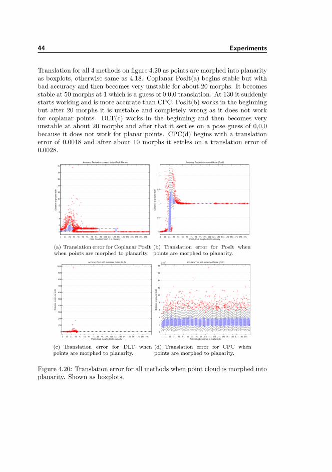
Translation for all 4 methods on figure 4.20 as points are morphed into planarityas boxplots, otherwise same as 4.18. Coplanar PosIt(a) begins stable but withbad accuracy and then becomes very unstable for about 20 morphs. It becomesstable at 50 morphs at 1 which is a guess of 0,0,0 translation. At 130 it suddenlystarts working and is more accurate than CPC. PosIt(b) works in the beginningbut after 20 morphs it is unstable and completely wrong as it does not workfor coplanar points. DLT(c) works in the beginning and then becomes veryunstable at about 20 morphs and after that it settles on a pose guess of 0,0,0because it does not work for planar points. CPC(d) begins with a translationerror of 0.0018 and after about 10 morphs it settles on a translation error of0.0028.
1 11 21 31 41 51 61 71 81 91 101 111 121 131 141 151 161 171 181 191
0
2
4
6
8
10
12
14
16
18
20
Dis
tanc
e to
gro
und
trut
h
Point cloud morphed in to planarity
Accuracy Test with increased Noise (PosIt Planar)
(a) Translation error for Coplanar PosItwhen points are morphed to planarity.
1 11 21 31 41 51 61 71 81 91 101 111 121 131 141 151 161 171 181 191
0
0.5
1
1.5
2
Dis
tanc
e to
gro
und
trut
h
Point cloud morphed in to planarity
Accuracy Test with increased Noise (PosIt)
(b) Translation error for PosIt whenpoints are morphed to planarity.
1 11 21 31 41 51 61 71 81 91 101 111 121 131 141 151 161 171 181 191
0
100
200
300
400
500
600
700
800
900
1000
Dis
tanc
e to
gro
und
trut
h
Point cloud morphed in to planarity
Accuracy Test with increased Noise (DLT)
(c) Translation error for DLT whenpoints are morphed to planarity.
1 11 21 31 41 51 61 71 81 91 101 111 121 131 141 151 161 171 181 191
0
2
4
6
8
10
12
14
16
18x 10
−3
Dis
tanc
e to
gro
und
trut
h
Point cloud morphed in to planarity
Accuracy Test with increased Noise (CPC)
(d) Translation error for CPC whenpoints are morphed to planarity.
Figure 4.20: Translation error for all methods when point cloud is morphed intoplanarity. Shown as boxplots.
4.1 Tests 45
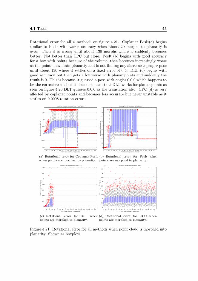
Rotational error for all 4 methods on figure 4.21. Coplanar PosIt(a) beginssimilar to PosIt with worse accuracy when about 20 morphs to planarity isover. Then it is wrong until about 130 morphs where it suddenly becomesbetter. Not better than CPC but close. PosIt (b) begins with good accuracyfor a box with points because of the volume, then becomes increasingly worseas the points move into planarity and is not finding anywhere near proper poseuntil about 130 where it settles on a fixed error of 0.4. DLT (c) begins withgood accuracy but then gets a lot worse with planar points and suddenly theresult is 0. This is because it guessed a pose with angles 0,0,0 which happens tobe the correct result but it does not mean that DLT works for planar points asseen on figure 4.20 DLT guesses 0,0,0 as the translation also. CPC (d) is veryaffected by coplanar points and becomes less accurate but never unstable as itsettles on 0.0008 rotation error.
1 11 21 31 41 51 61 71 81 91 101 111 121 131 141 151 161 171 181 191
−1
−0.5
0
0.5
1
1.5
Dis
tanc
e to
gro
und
trut
h(ro
t)
Point cloud morphed in to planarity
Accuracy Test with increased Noise (PosIt Planar)
(a) Rotational error for Coplanar PosItwhen points are morphed to planarity.
1 11 21 31 41 51 61 71 81 91 101 111 121 131 141 151 161 171 181 191
0
0.2
0.4
0.6
0.8
1
1.2
1.4
1.6
1.8
Dis
tanc
e to
gro
und
trut
h(ro
t)
Point cloud morphed in to planarity
Accuracy Test with increased Noise (posit)
(b) Rotational error for PosIt whenpoints are morphed to planarity.
1 11 21 31 41 51 61 71 81 91 101 111 121 131 141 151 161 171 181 191
0
0.2
0.4
0.6
0.8
1
1.2
1.4
Dis
tanc
e to
gro
und
trut
h(ro
t)
Point cloud morphed in to planarity
Accuracy Test with increased Noise (DLT)
(c) Rotational error for DLT whenpoints are morphed to planarity.
1 11 21 31 41 51 61 71 81 91 101 111 121 131 141 151 161 171 181 191
0
0.5
1
1.5
2
2.5
3
3.5
4
4.5
x 10−3
Dis
tanc
e to
gro
und
trut
h(ro
t)
Point cloud morphed in to planarity
Accuracy Test with increased Noise (CPC)
(d) Rotational error for CPC whenpoints are morphed to planarity.
Figure 4.21: Rotational error for all methods when point cloud is morphed intoplanarity. Shown as boxplots.
46 Experiments
Conclusion must be that PosIt for planar points must have a planar object andnot an object that is almost planar. PosIt for coplanar points is more accuratethan CPC, PosIt and DLT and even with more iterations CPC can not get moreaccurate than it is considering translation error. CPC is still more accurate whenit comes to rotational error. This shows that for planar points the planar versionof PosIt is the better choice.
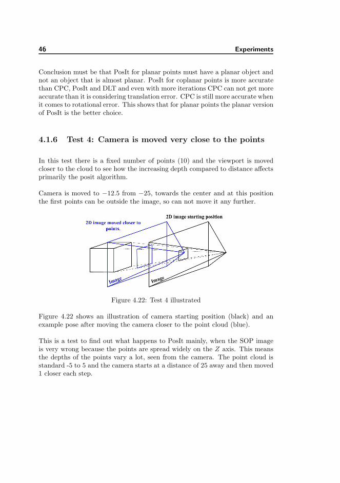
4.1.6 Test 4: Camera is moved very close to the points
In this test there is a fixed number of points (10) and the viewport is movedcloser to the cloud to see how the increasing depth compared to distance affectsprimarily the posit algorithm.
Camera is moved to −12.5 from −25, towards the center and at this positionthe first points can be outside the image, so can not move it any further.
Figure 4.22: Test 4 illustrated
Figure 4.22 shows an illustration of camera starting position (black) and anexample pose after moving the camera closer to the point cloud (blue).
This is a test to find out what happens to PosIt mainly, when the SOP imageis very wrong because the points are spread widely on the Z axis. This meansthe depths of the points vary a lot, seen from the camera. The point cloud isstandard -5 to 5 and the camera starts at a distance of 25 away and then moved1 closer each step.
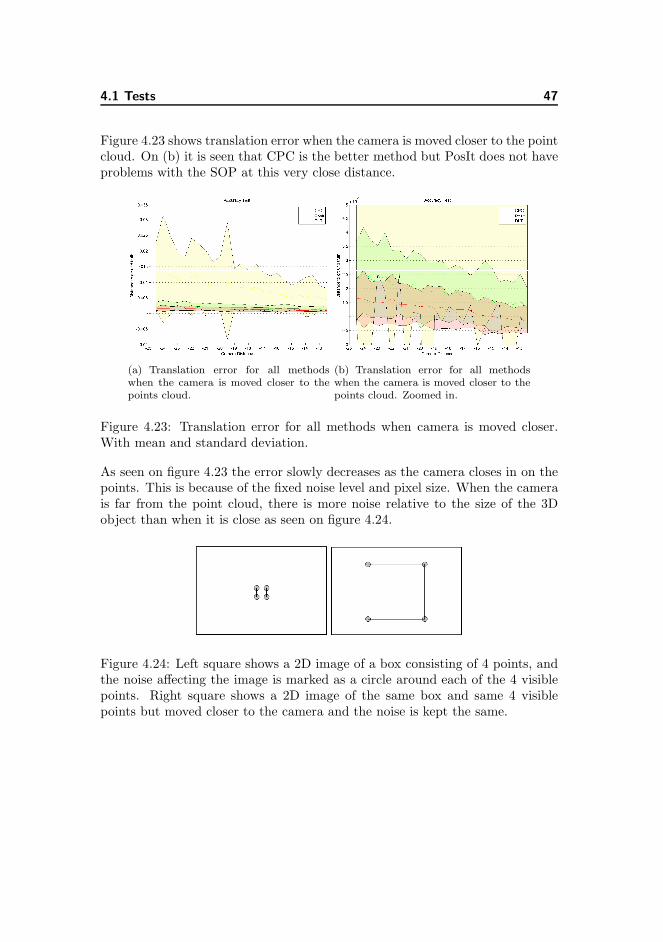
4.1 Tests 47
Figure 4.23 shows translation error when the camera is moved closer to the pointcloud. On (b) it is seen that CPC is the better method but PosIt does not haveproblems with the SOP at this very close distance.
(a) Translation error for all methodswhen the camera is moved closer to thepoints cloud.
(b) Translation error for all methodswhen the camera is moved closer to thepoints cloud. Zoomed in.
Figure 4.23: Translation error for all methods when camera is moved closer.With mean and standard deviation.
As seen on figure 4.23 the error slowly decreases as the camera closes in on thepoints. This is because of the fixed noise level and pixel size. When the camerais far from the point cloud, there is more noise relative to the size of the 3Dobject than when it is close as seen on figure 4.24.
Figure 4.24: Left square shows a 2D image of a box consisting of 4 points, andthe noise affecting the image is marked as a circle around each of the 4 visiblepoints. Right square shows a 2D image of the same box and same 4 visiblepoints but moved closer to the camera and the noise is kept the same.
48 Experiments
−24 −23 −22 −21 −20 −19 −18 −17 −16 −15 −14 −13
0
1
2
3
4
5
6
7x 10
−3
Dis
tanc
e to
gro
und
trut
h
Distance from camera to points
Accuracy Test with points moved closer(CPC)
(a) CPC translation error for cameramoved closer to point cloud.
−24 −23 −22 −21 −20 −19 −18 −17 −16 −15 −14 −13
0
1
2
3
4
5
6
7
8
9
x 10−3
Dis
tanc
e to
gro
und
trut
h
Distance from camera to points
Accuracy Test with points moved closer(POSIT)
(b) PosIt translation error for cameramoved closer to point cloud.
−24 −23 −22 −21 −20 −19 −18 −17 −16 −15 −14 −13
0
0.02
0.04
0.06
0.08
0.1
0.12
0.14
0.16
0.18
Dis
tanc
e fr
om to
poi
nts
Distance from camera to points
Accuracy Test with points moved closer(DLT)
(c) DLT translation error for cameramoved closer to point cloud.
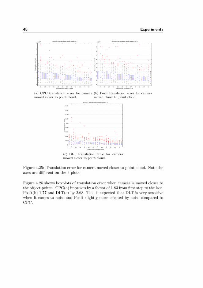
Figure 4.25: Translation error for camera moved closer to point cloud. Note theaxes are different on the 3 plots.
Figure 4.25 shows boxplots of translation error when camera is moved closer tothe object points. CPC(a) improves by a factor of 1.83 from first step to the last.PosIt(b) 1.77 and DLT(c) by 2.68. This is expected that DLT is very sensitivewhen it comes to noise and PosIt slightly more effected by noise compared toCPC.
4.1 Tests 49
−24 −23 −22 −21 −20 −19 −18 −17 −16 −15 −14 −13
0
0.5
1
1.5
2
x 10−3
Dis
tanc
e to
gro
und
trut
h(ro
t)
Distance from camera to points
Accuracy Test with points moved closer (CPC)
(a) CPC rotation error for cameramoved closer to point cloud.
−24 −23 −22 −21 −20 −19 −18 −17 −16 −15 −14 −13
0
0.5
1
1.5
2
2.5
3x 10
−3
Dis
tanc
e to
gro
und
trut
h(ro
t)
Distance from camera to points
Accuracy Test with points moved closer(POSIT)
(b) PosIt translation error for cameramoved closer to point cloud.
−24 −23 −22 −21 −20 −19 −18 −17 −16 −15 −14 −13
0
0.01
0.02
0.03
0.04
0.05
0.06
0.07
Dis
tanc
e to
gro
und
trut
h(ro
t)
Distance from camera to points
Accuracy Test with points moved closer(DLT)
(c) DLT translation error for cameramoved closer to point cloud.
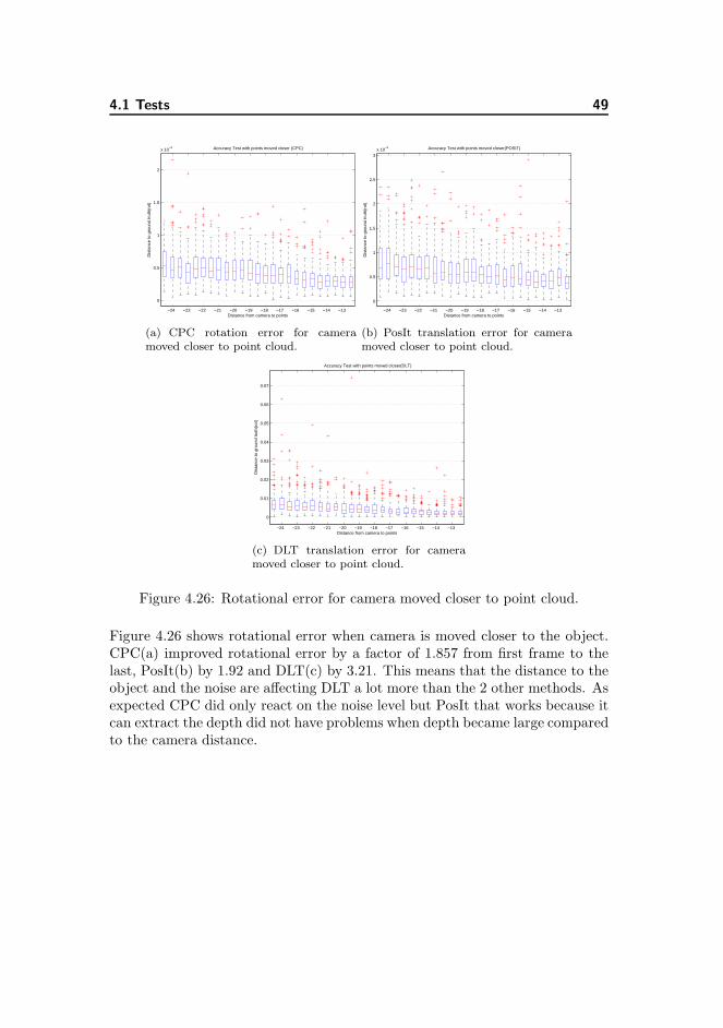
Figure 4.26: Rotational error for camera moved closer to point cloud.
Figure 4.26 shows rotational error when camera is moved closer to the object.CPC(a) improved rotational error by a factor of 1.857 from first frame to thelast, PosIt(b) by 1.92 and DLT(c) by 3.21. This means that the distance to theobject and the noise are affecting DLT a lot more than the 2 other methods. Asexpected CPC did only react on the noise level but PosIt that works because itcan extract the depth did not have problems when depth became large comparedto the camera distance.
50 Experiments
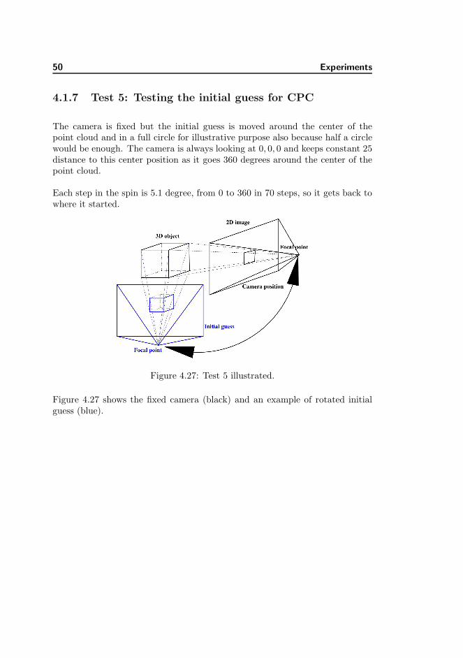
4.1.7 Test 5: Testing the initial guess for CPC
The camera is fixed but the initial guess is moved around the center of thepoint cloud and in a full circle for illustrative purpose also because half a circlewould be enough. The camera is always looking at 0, 0, 0 and keeps constant 25distance to this center position as it goes 360 degrees around the center of thepoint cloud.
Each step in the spin is 5.1 degree, from 0 to 360 in 70 steps, so it gets back towhere it started.
Figure 4.27: Test 5 illustrated.
Figure 4.27 shows the fixed camera (black) and an example of rotated initialguess (blue).
4.1 Tests 51
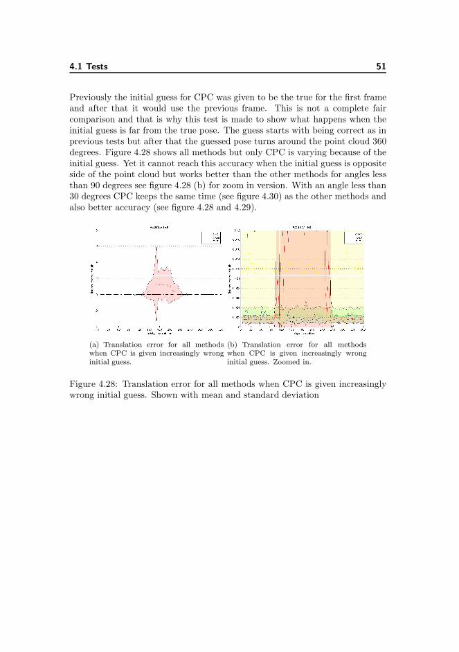
Previously the initial guess for CPC was given to be the true for the first frameand after that it would use the previous frame. This is not a complete faircomparison and that is why this test is made to show what happens when theinitial guess is far from the true pose. The guess starts with being correct as inprevious tests but after that the guessed pose turns around the point cloud 360degrees. Figure 4.28 shows all methods but only CPC is varying because of theinitial guess. Yet it cannot reach this accuracy when the initial guess is oppositeside of the point cloud but works better than the other methods for angles lessthan 90 degrees see figure 4.28 (b) for zoom in version. With an angle less than30 degrees CPC keeps the same time (see figure 4.30) as the other methods andalso better accuracy (see figure 4.28 and 4.29).
(a) Translation error for all methodswhen CPC is given increasingly wronginitial guess.
(b) Translation error for all methodswhen CPC is given increasingly wronginitial guess. Zoomed in.
Figure 4.28: Translation error for all methods when CPC is given increasinglywrong initial guess. Shown with mean and standard deviation
52 Experiments
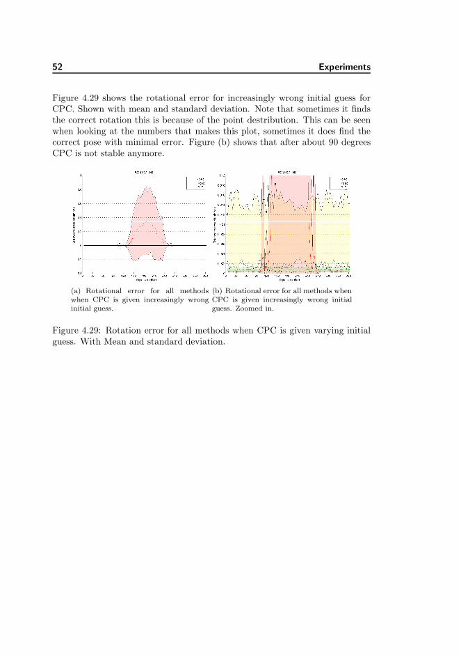
Figure 4.29 shows the rotational error for increasingly wrong initial guess forCPC. Shown with mean and standard deviation. Note that sometimes it findsthe correct rotation this is because of the point destribution. This can be seenwhen looking at the numbers that makes this plot, sometimes it does find thecorrect pose with minimal error. Figure (b) shows that after about 90 degreesCPC is not stable anymore.
(a) Rotational error for all methodswhen CPC is given increasingly wronginitial guess.
(b) Rotational error for all methods whenCPC is given increasingly wrong initialguess. Zoomed in.
Figure 4.29: Rotation error for all methods when CPC is given varying initialguess. With Mean and standard deviation.
4.1 Tests 53
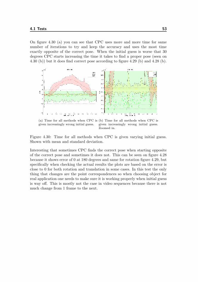
On figure 4.30 (a) you can see that CPC uses more and more time for samenumber of iterations to try and keep the accuracy and uses the most timeexactly opposite of the correct pose. When the initial guess is worse that 30degrees CPC starts increasing the time it takes to find a proper pose (seen on4.30 (b)) but it does find correct pose according to figure 4.29 (b) and 4.28 (b).
(a) Time for all methods when CPC isgiven increasingly wrong initial guess.
(b) Time for all methods when CPC isgiven increasingly wrong initial guess.Zoomed in.
Figure 4.30: Time for all methods when CPC is given varying initial guess.Shown with mean and standard deviation.
Interesting that sometimes CPC finds the correct pose when starting oppositeof the correct pose and sometimes it does not. This can be seen on figure 4.28because it shows error of 0 at 180 degrees and same for rotation figure 4.29, butspecifically when checking the actual results the plots are based on the error isclose to 0 for both rotation and translation in some cases. In this test the onlything that changes are the point correspondences so when choosing object forreal application one needs to make sure it is working properly when initial guessis way off. This is mostly not the case in video sequences because there is notmuch change from 1 frame to the next.
54 Experiments
4.1.8 Test 6: Different implementation of PosIt
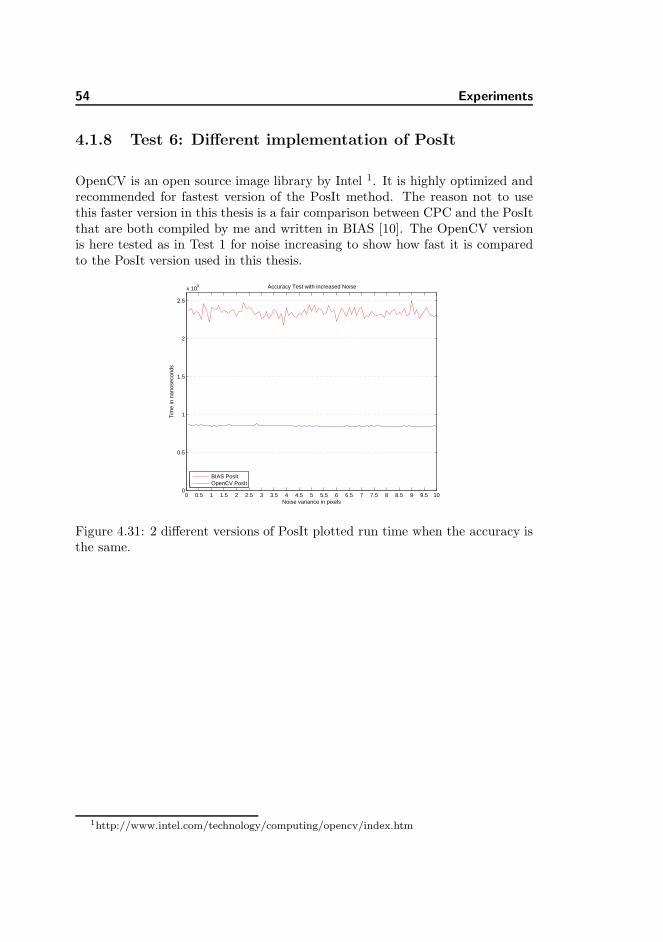
OpenCV is an open source image library by Intel 1. It is highly optimized andrecommended for fastest version of the PosIt method. The reason not to usethis faster version in this thesis is a fair comparison between CPC and the PosItthat are both compiled by me and written in BIAS [10]. The OpenCV versionis here tested as in Test 1 for noise increasing to show how fast it is comparedto the PosIt version used in this thesis.
0 0.5 1 1.5 2 2.5 3 3.5 4 4.5 5 5.5 6 6.5 7 7.5 8 8.5 9 9.5 100
0.5
1
1.5
2
2.5
x 105 Accuracy Test with increased Noise
Noise variance in pixels
Tim
e in
nan
osec
onds
BIAS PosItOpenCV PosIt
Figure 4.31: 2 different versions of PosIt plotted run time when the accuracy isthe same.
1http://www.intel.com/technology/computing/opencv/index.htm

4.1 Tests 55
Figure 4.31 shows PosIt from BIAS and PosIt from OpenCV with mean timefor the same number of iterations over 100 runs as the noise increases (noise isnot relevant but the test is taken from Test 1). OpenCV PosIt has an averagetime of 0.849 ms and the BIAS version has 2.34 ms that is 2.7 times slower butotherwise they are exactly the same. CPC could be optimized as well for betterperformance by using a different compiler or different compiler settings. Butusing the slower version will keep the methods comparable.

56 Experiments
Chapter 5
Conclusion
Gauss-Newton with Levenberg-Marquardt modification, PosIt, PosIt for copla-nar points and finally the direct linear transform has been tested in variousextremes to reveal positive and negative sides.
First was tested how they were affected by noise. Then tested what happenswhen more point correspondences are added. And tested what happens whenthe object is at the limit of planarity. Then tested what happens when theobject is close to the camera. Finally tested what happens when initial guess isvery bad for iterative method CPC.
CPC is iterative and relies on minimizing the back projected error of a posewhen changing the parameters of the projection matrix according to first orderderivatives of the residual and the approximated hessian without the secondorder derivatives which is considered time consuming.
PosIt is approximating the depth in the image for every 2D point it has corre-spondence for, starting from pure orthographic projection and then iterativelyimproves this to estimate perspective projection.
The planar version of PosIt works like PosIt except it finds 2 rotation matricesfor every previous found pose and keeps choosing the better 2 poses. Ending upwith 2 poses instead of 1 like PosIt.
58 Conclusion
DLT uses SVD to linearly find the 11 parameters of the projection matrix andtherefore requires more points than the other methods and it also has otherdrawbacks, but it is used as comparison for the other methods.
Noise affect the methods very differently, as expected DLT is the worst but CPCis slightly better than PosIt handling noise. This is important if the noise levelin a practical application is really high it might not work accurate enough.
When the methods get more point correspondences it mostly affect DLT thatincreased run time by a factor 8, CPC only with a factor of 1.84 and PosIt inthe middle with a factor of 2.76.
Interestingly the planarity was affecting all the methods in some way. MostlyPosIt which error slowly increased as the object became planar. And the planarversion of PosIt that did not work at all for near planar objects but gave a decentguess for objects with volume, meaning it worked for planar objects and non-planar but not the transition between these. And CPC became less accuratewhen the object was planar.
Important thing about CPC is the initial guess and as proven in Test 5 the pointdistribution determines how well the initial guess have to be. Also shown is thatthe initial guess has to deviate more than 30 degrees before anything happensto the run time of CPC.
-CPC is best when you got a movie sequence and know the pose from the lastframe, it is very accurate but can give very wrong results if the initial guess ismore off than 90 degrees.
-PosIt has the drawback of coplanar points but it is almost as fast as CPC anddoes not require initial guess which means it is perfect if you got 1 image ofpoints that are sure not to be coplanar.
-Coplanar PosIt is just as fast and more accurate for translation error comparedto CPC in the case where points are coplanar, it can also give a valuable clueto how likely the pose is to be the right one by providing the 2 best posespossible. This is unique for this method and cannot be done by either of theother methods. Negative that it needs perfectly 2D marker as in ARToolKit.
-DLT was used as a comparator for the other methods. If the 2D-3D correspon-dences are without noise the DLT works good but extreme sensitivity to noisemakes it a bad choice for any real application.

Appendix A
The Test Program
Because the methods are implemented in C++ it is natual to write the testingprogram in that lagnauge also. The values from each test is stored in *.txt andread by a Matlab program that draws the graphs. Here is a description of allfunctions in C++ and their usage.
void init() -Initializes camera position, kalibration matrix and glut camera set-tings.
void drawFloor(float size, int nrQuadsPerRow) -Makes a green square in themiddle of the points with size 10x10 to give a better 3D effect.
void drawPoint() -Draws 1 point at the current position.
void display() -Glut draws the scene with objects.
void reshape(int w, int h) -Resets the glut camera settings.
void SaveData(const char* file, int type,int x, int y) -Saves the translation error,rotation error and run time for last run method to *.txt.
void SavePMatrix() -Stores correct projection matrices for each frame to makeground truth for comparison.
60 The Test Program
void AddNoise() -2D points made from ground truth projection of the 3D objectis added noise.
void AddPlanarMovement() -3D points are morphed 30% closer to planarityparallel to image plane.
void AddPlanarMovement2() - 3D points are morphed in the diagonal 30%towards planarity, angled 0.25 π.
void ProjectPointsTruth() - Projects the 3D object points with ground truthprojection matrix to make perfect 2D points.
void CamPoseCalib algo() -Gauss-Newton method. Fills matrices with transla-tion, rotation error and the run time.
void CamPoseCalib algo time(float time limit) -Sets a time limit for CPC so itincreases/decreases number of iteration until it reaches the desired run time.
void OpenCVPoseIT() -PosIt method from OpenCV. Fills matrices with trans-lation, rotation error and the run time.
void OpenCVPoseIT time(float time limit) -Sets a time limit for PosIt so itincreases/decreases number of iteration until it reaches the desired run time.
void PositWithPlanar() -Both PosIt and PosIt for coplanar points depending onthe variable ”dim”. When dim is 3, it means the points are spread in 3D and itwill use PosIt. If dim is 2, it means the points are on a plane and it runs planarversion of PosIt.
void ARToolkit() -ARToolKit not used.
double arGetTransMatT( ) -ARToolKit not used.
double arGetTransMat2T( double rot[3][3], double ppos2d[][2], double ppos3d[][3],int num ) -ARToolKit not used.
double arGetTransMat3T( double rot[3][3], double ppos2d[][2], double ppos3d[][3],int num, double *dist factor, double cpara[3][4] ) -ARToolKit not used.
double arGetTransMat4T( double rot[3][3], double ppos2d[][2], double ppos3d[][3],int num ) -ARToolKit not used.
double arGetTransMat5T( double rot[3][3], double ppos2d[][2], double ppos3d[][3],int num, double *dist factor, double cpara[3][4] ) -ARToolKit not used.
61
static double arGetTransMatSubT( double rot[3][3], double ppos2d[][2], doublepos3d[][3], int num, double *dist factor, double cpara[3][4] ) -ARToolKit notused.
void DLT() -Direct Linear transform method. Fills matrices with translation,rotation error and the run time.
void keyPressed(unsigned char key, int x, int y) -Starts the test chosen when”f” is pressed. Single methods can be tested with ”i”.
void animation() -Can make things rotate. Not used.
void mousePressed(int button, int state, int x, int y) -Used to move the glutcamera for viewing the points and camera.
void mouseMotion(int x, int y) -If mouse pressed it can rotate the glut camera.
void noiseTest time() -Test 1 with fixed time.
void noiseTest acc() -Test 1 with different number of iterations.
void createSamples() -Creates array with 60 3D points randomly between -5 and+5 on all 3 axes.
int main(int argc, char** argv) -Sets window size and position. Initaializes theglut functions for viewing color 3D and more.

62 The Test Program
Bibliography
[1] Y. Abdel-Aziz and H. Karara. Direct linear transformation from compara-tor coordinates into object space coordinates in close-range photogramme-try. pages 1–18, 1971.
[2] Ronald T. Azuma. A survey of augmented reality. 6 (4), 1997. HughesResearch Laboratories 3011 Malibu Canyon Road, MS RL96 Malibu, CA90265.
[3] Helder Araujo Rodrigo L. Carceroni Christopher M. Brown. A fully pro-jective formulation for lowe’s tracking alogrithm. pages 227–238, 1998.
[4] Edwin K. P. Chong and Stanislaw H. Zak. An Introduction to Optimization.John Wiley & Sons, 2001.
[5] D. Oberkampf & L. S. Davis Daniel DeMenthon. Iterative pose estimationusing coplanar feature points. 63 (nr. 3), 1996.
[6] Daniel F. DeMenthon & Larry S. Davis. Model-based object pose in 25lines of code. International Journal of Computer Vision, 15:123–141, 1995.
[7] Philip David Daniel DeMenthon Ramani Duraiswami and Hanan Samet.Simultaneous pose and correspondence determination. pages 698–714, 2002.
[8] Vincent Lepetit & Pascal Fua Francesc Moreno-Noguer. Accurate non-iterative o(n) solution to the pnp problem. ICCV07(1-8), 2007.
[9] Daniel Grest. Marker-free human motion capture in dynamic clutteredenvironments from a single view-point. 2007.

64 BIBLIOGRAPHY
[10] J. F. Evers-Senne J. M. Frahm D. Grest K. Koser B. Streckel J. Bias (basicimage algorithms). 2006.
[11] Hirokazu Kato and Mark Billinghurst. Marker tracking and hmd calibrationfor a video-based augmented reality conferencing system. IWAR ’99, SanFrancisco, pages 85–94, 1999.
[12] Vincent Lepetit and Pascal Fua. Monocular model-based 3d tracking ofrigid objects: A survey. 1(1), 2005. Computer Vision Laboratory, CH-1015Lausanne, Switzerland.
[13] Z. Zhang. Flexible camera calibration by viewing a plane from unknownorientations. pages 666–673, 1999. Corfu Greece.
Related Documents

![DeepIM: Deep Iterative Matching for 6D Pose Estimation · RGB based 6D Pose Estimation: Traditionally, pose estimation using RGB im-ages is tackled by matching local features [16,23,4].](https://static.cupdf.com/doc/110x72/5f53ae335b64ec19467e81ba/deepim-deep-iterative-matching-for-6d-pose-estimation-rgb-based-6d-pose-estimation.jpg)

![Conservative Wasserstein Training for Pose Estimation...classification-regression framework for 3d pose estimation from 2d images. BMVC, 2018. 1, 2, 8 [38] FranciscoMassa,RenaudMarlet,andMathieuAubry.](https://static.cupdf.com/doc/110x72/5faa9b1f951401416a277528/conservative-wasserstein-training-for-pose-estimation-classiication-regression.jpg)


![[DL輪読会] Realtime Multi-Person 2D Pose Estimation using Part Affinity Fields](https://static.cupdf.com/doc/110x72/5a65d16e7f8b9ad02f8b4771/dl-realtime-multi-person-2d-pose-estimation-using-part-affinity.jpg)