A Comparative Simulation Study of Link Quality Estimators in Wireless Sensor Networks

A Comparative Simulation Study of Link QualityEstimators in Wireless Sensor Networks

Nouha Baccour∗ †, Anis Koubaa† ‡, Maissa Ben Jamaa∗, Habib Youssef§, Marco Zuniga¶, and Mario Alves†

∗ReDCAD Research Unit, National school of Engineers of Sfax,B.P.W 3038, Sfax, Tunisia.

†IPP-HURRAY! Research Group, Polytechnic Institute of Porto,Rua Antnio Bernardino de Almeida, 431, 4200-072 Porto, Portugal.

‡Al-Imam Mohamed bin Saud University,College of Computer Science and Information Systems,

KSA 96678-2391,Riyadh, Saudi Arabia.§Prince Research Unit, University of Sousse, Sousse, Tunisia.

¶Tyrell Inc.,123 Replicant Street, Los Angeles, California 902104321.

Emails:{nabr,aska}@isep.ipp.pt, [email protected], [email protected], [email protected], [email protected]

Abstract—Link quality estimation (LQE) in wireless sensornetworks (WSNs) is a fundamental building block for an efficientcross-layer design of higher layer wireless network protocols. Sev-eral link quality estimators have been reported in the literature;however, none of the proposed estimators have been the subject ofa thorough evaluation. Further, there is a need for a comparativestudy of these estimators as well as the assessment of the impactof each on higher layer protocols. In this work, we performan extensive comparative simulation study among the well-known link quality estimators using TOSSIM simulator. We firstanalyze the statistical properties of the link quality estimatorsindependently of higher-layer protocols, then we investigate theirimpact of the Collection Tree Routing protocol (CTP). We believethat this work provides a fundamental step in understandingthe statistical behavior of LQE techniques, which helps networkdesigners to choose the most appropriate one for their higher-layer protocols.

I. I NTRODUCTION

Wireless communication links are known to be unreliableas their behavior unpredictably varies over time and space.Links unreliability poses a major handicap for self-organizingwireless networks, such as sensor, ad-hoc and mesh networks,for maintaining their correct behavior, unless it is taken intoaccount by higher layer communication protocols. Particularly,sophisticated routing protocols aim to overcome link unrelia-bility in order to efficiently maintain network connectivity. Toachieve this goal, they rely on link quality estimation (LQE)as a support mechanism to select the most stable routes fordata delivery [1]–[4]. Stable routes are built by selecting linkswith the highest quality and discarding those of bad quality.Building such routes will definitely improve the networkthroughput and maximize its lifetime. In fact, data deliveryover stable routes has the advantage of (i.) increasing the end-to-end probability of delivery rate, which infer on the accuracy(ii.) avoiding excessive re-transmissions over low quality linksand thus to considerably reduce energy consumption at eachnode performing its routing task, which infers on the cost,

(iii. ) minimizing the route re-selection operation triggered bylinks failure, which infers on the stability. The accuracy ofthe link quality estimate will impact the goodness-of-decisionmade by routing protocols in selecting stable routes. The moreaccurate the estimate is, the more stable routes will be, andthis improves delivery rates. Therefore, accurate link qualityestimate is a prerequisite for efficient routing mechanisms thatmanage to overcome problems imposed by link unreliability.

In Wireless Sensor Networks (WSNs), link quality estima-tion is more challenging than in the other traditional wirelessmesh and ad-hoc networks, because sensor nodes are denselydeployed and basically use low-power radios. It has beenexperimentally shown that low-power radios are more prone tonoise, interference, and multipath distortion [5]. As a result,communication links in WSNs exhibit more unreliability ascompared to those of traditional mesh and ad-hoc networks[5]–[11].

Link quality estimation in WSNs is still an open researchchallenge, although there have been several recent works thathave introduced new LQE metrics for sensor networks [6],[12]–[15] and others have assessed the convenience of tradi-tional estimation metrics for sensor networks [16]. However,none of the proposed link quality estimators have been thesubject of a thorough evaluation.

In this paper, we conduct a comparative simulation study oflink quality estimators. We particularly present an extensiveperformance evaluation of five existing link quality estimatorsfor wireless sensor networks:PRR, WMEWMA, RNP, ETXandFour-Bit.

II. RELATED WORK

In this section, we briefly review the literature related tolink quality estimators in WSNs, as well as their performanceevaluation.

A. Link Quality Estimators

Link quality estimators in wireless sensor networks canroughly be classified in two categories: hardware-based es-timators and software-based estimators.

Hardware-based estimators include Link Quality Indicator(LQI) Received Signal Strength Indicator (RSSI) and Signal-to-Noise Ratio (SNR). These estimators are directly obtainedfrom the hardware, namely CC2420 radio transceiver [17].Their advantage is that they do not require any computationoverhead as they are built-in directly on the hardware. How-ever, as it was observed and reported in pervious experimentalstudies, hardware-based estimators do not provide accurateestimate [13], [18], [19], mainly for the following reasons:First, these metrics are measured based on 8 symbols ofa received packet and not the whole packet. Second, thesemetrics are only measured for successfully received packets.Therefore, when a radio link suffers from excessive packetloss, they could overestimate the transmission performance bynot considering the information of lost packets.

On the other hand, Software-based estimators enable tocount or approximateeither (i.) the reception rate, or (ii.)the average number of packet transmissions/re-transmissions,required before its successful reception.The Packet Reception Rate (PRR) and the Acquitted ReceptionRate (ARR) count the reception rate. The first is performed atthe receiver side and the second at the sender side. These linkquality estimators are simple, yet they have been widely usedin routing protocols (e.g. in [20]).The Required Number of Packet transmissions (RNP) countsthe average number of packet transmissions/re-transmissions,required before its successful reception. It is introduced byCerpa et.al. In [6], the authors argue thatRNP is better thanPRRfor characterizing the link quality becausePRRprovides acoarse-grain estimation of the link quality since it does not takeinto account the underlying distribution of losses, in contrastto RNP.The Window Mean with Exponentially Weighted MovingAverage (WMEWMA) [12], the Kalman filter based linkquality estimator [15]and the packet success probability (PSP)[10], approximate the packet reception rate.Furthermore, the link inefficiency metric (LI) [13], expectedtransmission count (ETX) [21], andFour-Bit [14]approximatethe average number of packet transmissions/re-transmissions,required before a successful reception.A through presentation of LQEs under evaluation will bepresented in Section 3.

B. Performance Evaluation of Link Quality Estimators

To the best of our knowledge, there is no previous compar-ative study of link quality estimators in WSNs other than [12]and [6].

In [12], the authors introduced the Window Mean with Ex-ponentially Weighted Moving Average (WMEWMA), a filter-based link quality estimator. The performance ofWMEWMAwas compared against other filter-based link quality estimators:Exponentially Weighted Moving Average (EWMA), Moving

Average (MA) and Time-Weighted Moving Average (TWMA).The comparative study conducted in [12] has the advan-tage that it takes into account various performance criteria.However, it is restricted to filter-based LQEs. Further, thecomparison is based on a simple generated trace, which doesnot take into account accurately the characteristics of channelcommunication. The trace generator is based on the assump-tion that packets transmission corresponds to independentBernoulli trials. Performance comparison between filter-basedLQEs is performed in terms of accuracy, agility, stability,history, and resource utilization. Accuracy is quantified bycomparing the measured link quality, and the estimated linkquality, using the Mean Square Error. Agility is the abilityto quickly react to persistent changes in link quality. It hasbeen measured by the settle time, which is defined as the timeneeded by the estimator to reach the measured value, withinan error bound of e. Stability is the ability to resist to transient(short-term) variations, also called fluctuations, in link quality.It is has been measured by the coefficient of variation, whichis defined as the ratio of the standard deviation to the mean.History refers to the time window used to produce the estimate.A larger history yields a more stable, but less agile estimator[12]. Finally, resource utilization refers to the computation andstorage overhead. Based on the above performance criteria,Woo et al. have shown thatWMEWMAperforms better thanthe other filter-based LQEs.

On the other hand, in [6]the main goal was to study thetemporal characteristics of low-power links, using a real de-ployment of a WSN. Meanwhile, the authors of [6] comparedPRR and RNP in order to select the suitable metric forlink characterization. Cerpa et al. argued thatRNP is betterthan PRR for estimating link quality. To justify their findingthe authors observed different links during several hours, bymeasuringPRRand RNP each one minute. They found thatfor bad-quality and good-quality links, i.e. links having high(>90%) and low reception rates (<50%) respectively,PRRfollows the same behaviour asRNP. However, for medium-quality links, PRR overestimates the link quality because itdoes not take into account the underlying distribution of packetlosses: when the link exhibits short periods during whichpackets are not received, thePRR can still have high valuebut theRNP is high so that it indicates the usefulness of thelink. As a matter of fact, a packet that cannot be deliveredis retransmitted many times before being abandoned. Theauthors of [6] also studied the relationship betweenRNPandthe inverse ofPRR(1/PRR) statistically by (i.) measuring thecumulative distribution function (CDF) ofRNPas a function of1/PRRand (ii.) measuring the Consistency level betweenRNPand 1/PRR. They found thatRNP and PRR are not directlyproportional.

III. STUDIED L INK QUALITY ESTIMATORS

In what follows, we present the different estimators underevaluation.TABLE I presents the most important characteris-tics of these estimators.

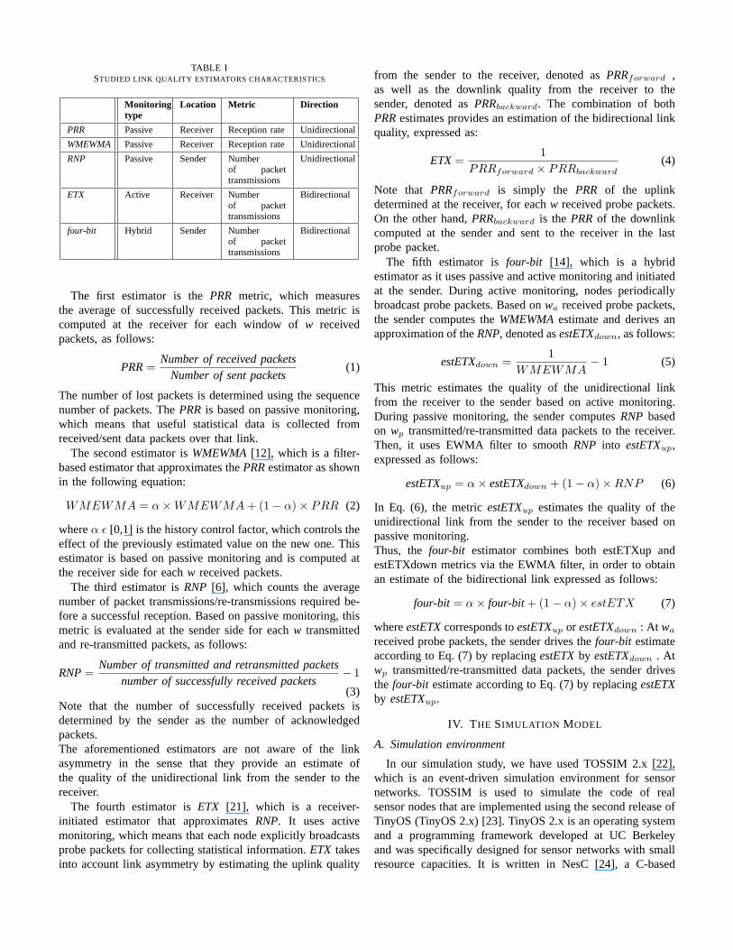
TABLE ISTUDIED LINK QUALITY ESTIMATORS CHARACTERISTICS

Monitoringtype

Location Metric Direction

PRR Passive Receiver Reception rate Unidirectional

WMEWMA Passive Receiver Reception rate Unidirectional

RNP Passive Sender Numberof packettransmissions

Unidirectional

ETX Active Receiver Numberof packettransmissions

Bidirectional

four-bit Hybrid Sender Numberof packettransmissions

Bidirectional

The first estimator is thePRR metric, which measuresthe average of successfully received packets. This metric iscomputed at the receiver for each window ofw receivedpackets, as follows:

PRR=Number of received packets

Number of sent packets(1)

The number of lost packets is determined using the sequencenumber of packets. ThePRR is based on passive monitoring,which means that useful statistical data is collected fromreceived/sent data packets over that link.

The second estimator isWMEWMA[12], which is a filter-based estimator that approximates thePRRestimator as shownin the following equation:

WMEWMA = α×WMEWMA + (1− α)× PRR (2)

whereα ε [0,1] is the history control factor, which controls theeffect of the previously estimated value on the new one. Thisestimator is based on passive monitoring and is computed atthe receiver side for eachw received packets.

The third estimator isRNP [6], which counts the averagenumber of packet transmissions/re-transmissions required be-fore a successful reception. Based on passive monitoring, thismetric is evaluated at the sender side for eachw transmittedand re-transmitted packets, as follows:

RNP=Number of transmitted and retransmitted packets

number of successfully received packets− 1

(3)Note that the number of successfully received packets isdetermined by the sender as the number of acknowledgedpackets.The aforementioned estimators are not aware of the linkasymmetry in the sense that they provide an estimate ofthe quality of the unidirectional link from the sender to thereceiver.

The fourth estimator isETX [21], which is a receiver-initiated estimator that approximatesRNP. It uses activemonitoring, which means that each node explicitly broadcastsprobe packets for collecting statistical information.ETX takesinto account link asymmetry by estimating the uplink quality

from the sender to the receiver, denoted asPRRforward ,as well as the downlink quality from the receiver to thesender, denoted asPRRbackward. The combination of bothPRRestimates provides an estimation of the bidirectional linkquality, expressed as:

ETX=1

PRRforward × PRRbackward(4)

Note that PRRforward is simply the PRR of the uplinkdetermined at the receiver, for eachw received probe packets.On the other hand,PRRbackward is the PRRof the downlinkcomputed at the sender and sent to the receiver in the lastprobe packet.

The fifth estimator isfour-bit [14], which is a hybridestimator as it uses passive and active monitoring and initiatedat the sender. During active monitoring, nodes periodicallybroadcast probe packets. Based onwa received probe packets,the sender computes theWMEWMAestimate and derives anapproximation of theRNP, denoted asestETXdown, as follows:

estETXdown =1

WMEWMA− 1 (5)

This metric estimates the quality of the unidirectional linkfrom the receiver to the sender based on active monitoring.During passive monitoring, the sender computesRNP basedon wp transmitted/re-transmitted data packets to the receiver.Then, it uses EWMA filter to smoothRNP into estETXup,expressed as follows:

estETXup = α× estETXdown + (1− α)×RNP (6)

In Eq. (6), the metricestETXup estimates the quality of theunidirectional link from the sender to the receiver based onpassive monitoring.Thus, the four-bit estimator combines both estETXup andestETXdown metrics via the EWMA filter, in order to obtainan estimate of the bidirectional link expressed as follows:

four-bit = α× four-bit + (1− α)× estETX (7)

whereestETXcorresponds toestETXup or estETXdown : At wa

received probe packets, the sender drives thefour-bit estimateaccording to Eq. (7) by replacingestETXby estETXdown . Atwp transmitted/re-transmitted data packets, the sender drivesthe four-bit estimate according to Eq. (7) by replacingestETXby estETXup.

IV. T HE SIMULATION MODEL

A. Simulation environment

In our simulation study, we have used TOSSIM 2.x [22],which is an event-driven simulation environment for sensornetworks. TOSSIM is used to simulate the code of realsensor nodes that are implemented using the second release ofTinyOS (TinyOS 2.x) [23]. TinyOS 2.x is an operating systemand a programming framework developed at UC Berkeleyand was specifically designed for sensor networks with smallresource capacities. It is written in NesC [24], a C-based

language that provides a support for the TinyOS componentand concurrency model.

One of the main reasons behind the use of TOSSIM 2 isthat it provides an accurate wireless channel model [25], [26],without which it will not be possible to consider the simulationresults as valid. In the following, we give a short overview onthis model.

In TOSSIM 2, the wireless channel model includes (i.) aradio propagation modeland (ii.) a link layer model. Theradio propagation model serves as input block for the linkquality model. As for radio propagation model, TOSSIM 2relies on thelog-normal shadowingpath loss model [27].On the other hand, the link layer model is given by ananalytical expression of thepacket reception probability(PRP)as a function of thesignal-to-noise ratio(SNR) [26]. Thismodel takes into account various parameters that affect thepacket delivery performance of low-power links [8], includinghardware calibration, the distance between nodes, the path lossmodel, etc. Therefore, based on these parameters, TOSSIM 2generates a link layer model (i.e.PRPas a function of theSNR)for each particular link in the sensor network. It also definesthe ”gain” of that link, which is the signal attenuation due tothe path loss. In addition, TOSSIM 2 uses a closest-fit patternmatching (CPM) model [25] to generate a distribution ofenvironment noise samples that captures temporal variation inthe environment. Whenever a simulated sensor node receivesa packet, it samples a noise reading (N) using the CPM modeland gathers the link gain (S) to determine theSNR(SNR=S/N).From the simulatedSNR value, the node determines thecorrespondingPRP using its link layer model. Based on thePRP, a node can decide whether a packet has been successfullyreceived or not. The interested reader can refer to [25], [26]for more details about the wireless channel model of TOSSIM2.

B. Reception region analysis

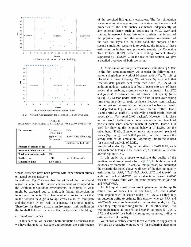
There have been several empirical studies that performedextensive measurements of low-power links quality, in orderto analyze their characteristics. Particularly, in [5], [7], [8],[10], link quality measurements have been carried out byobserving thePRRbetween a pair of nodes placed at differentdistances. The goal was to observe the evolution of thePRRasa function of the distance. Based on these measurements, threedifferent reception regions have been distinguished:connected,transitional, and disconnected. The connected region is theclosest to the receiver. It is characterized by consistently highreception rates, i.e. greater than 90%, for most of the links.In contrast, the disconnected region, which is the farthest tothe receiver, is identified by consistently low reception rates,which do not exceed 10%. In between, the transitional region,also referred to ”gray area”, is often quite large in widthas compared to both other regions. In this region, receptionrates are moderate, i.e. between 10% and 90%, and with highvariance, which implies the existence ofmoderate quality,instable, andasymmetriclinks.

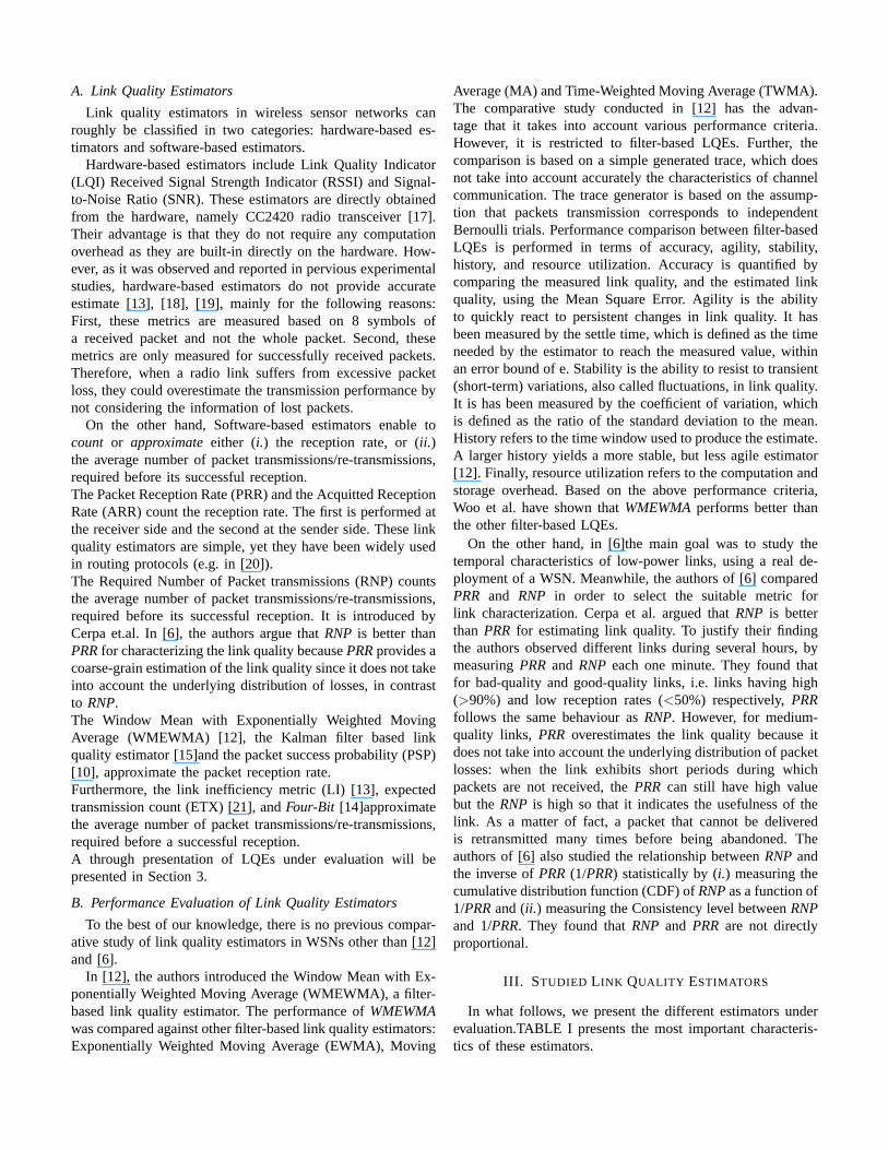
Fig. 1. Network Configuration for Reception Regions Evaluation

In order to properly configure the simulation models (referto Section 4.3), it was necessary to identify the three receptionregions in the simulated sensor network. In fact, the generalmethodology that we adopt for LQEs performance comparisonis (i.) to inject to each LQE a number of links, with differentcharacteristics, i.e. links of the connected region, others ofthe transitional region and others of the disconnected region,and (ii.) comparing the ability of LQEs to estimate the qualityof these links efficiently. Therefore, it is necessary to knowthe boundaries of the three reception regions in order to setthe distance between the sender and the receiver constitutingthe given link to estimate. In addition, as we consider twoenvironment types: (i.) an indoor environment (aisle of abuilding) [28], and (ii.) an outdoor environment (football field)[28], it is also mandatory to analyze the three reception regionsfor each of these environments.

For that purpose, we placed 60 sensor nodes around onesink node, as illustrated in Fig. 1. These sensor nodes weredivided in 10 sets, where each set contain 6 nodes, all placedin a circle around the sink node. The distance between twoconsecutive circles is equal to 1 meter. The first circle, i.e. thenearest to the sink, is placed at a distance to the sink node,equal tox meters. Each sensor node has an exclusive timeslot during which it sends 200 data packets to the sink node.Note that sensor nodes send their data in non overleaping timeslots in order to avoid collisions between sent packets. Further,packet retransmission mechanism has been activated.

For the outdoor environment, we simulated several scenarioswhile varying x in the set 1, 1.25, 1.5, 1.75 meter, whereasx has been varied in the set 1, 10, 20, 30 meter for theindoor environment. Simulation parameters are presented inTABLE II.

Fig. 2 presents thePRR as a function of the distance forboth indoor and outdoor environments, where it is possible toobserve the bounds of the three reception regions: connected,transitional and disconnected.It is important to note that the Fig. 2 proves the accuracy of thewireless channel model of TOSSIM. In fact, the majority ofnetwork simulators use an ideal link layer model [29] accord-ing which there are only two reception regions: connected anddisconnected. On the other hand, TOSSIM uses a realistic linkquality model because it leads to the three reception regions,

0,6

0,7

0,8

0,9

1Indoor

0

0,1

0,2

0,3

0,4

0,5

1 3 5 7 9 11 13 15 17 19 21 23 25 27 29 31 33 35 37 39

PRR

Distance

Connected Transitional Disconnected

(a) Indoor environment: aisle of building

1

0,8

0,9

1

0,5

0,6

0,7

PRR

Connected Transitional Disconnected

0,2

0,3

0,4Connected Transitional Disconnected

0

0,1

1 2 3 4 5 6 7 8 9 10

Di tDistance

(b) Outdoor environment: football field

Fig. 2. Network Configuration for Reception Regions Evaluation

TABLE IISIMULATION PARAMETERS FOR THE RECEPTION REGION EVALUATION

Environment Asymmetrylevel of links

High

Type of theEnvironment

Indoor: Aisle of building

Outdoor: Football field

Number of sensor nodes 61

Number of data sources 60

Total sent packets / node 200

Traffic type CBR rate: 61/8 packet/s

Simulation time 1700 ticks/s

whose existence have been proven with experimental studieson actual sensor networks.In addition, Fig. 2 shows that the width of the transitionalregion is larger in the indoor environment as compared tothe width in the outdoor environments, in contrast to whatmight be expected due to multipath fading, dispersion, inindoor environments. This phenomenon is due to the fact thatin the football field grass foliage creates a lot of multipathand dispersion which leads to a narrow transitional region.Therefore, for these particular environments, link qualities inthe football field will be worse than in the aisle of building.

C. Simulation studies

In this section, we describe both simulation scenarios thatwe have designed to evaluate and compare the performance

of the pre-cited link quality estimators. The first simulationscenario aims at analyzing and understanding the statisticalproperties of the link quality estimators independently ofany external factor, such as collisions in MAC layer androuting in network layer. We only consider the impact ofthe physical layer and the re-transmission mechanism ofthe data link layer. On the other hand, the purpose of thesecond simulation scenario is to evaluate the impact of theseestimators on higher layer protocols, namely the CollectionTree Protocol (CTP), which is a routing protocol alreadysupported by TOSSIM 2. In the rest of this section, we givea detailed overview of both scenarios.

1) First simulation study: Performance Evaluation of LQEs:In the first simulation study, we consider the following sce-nario: a single-hop network of 10 sensor nodes (N1, N2. . .N10)placed in a linear topology. We set nodeN1 as a sink thatreceives data packets sent from each node (N2. . .N10). Inaddition, nodeN1 sends a data flow of packets to each of thesenodes, thus enabling asymmetry-aware estimators, i.e.ETXand four-bit, to estimate the bidirectional link quality (referto Fig. 3). Sensor nodes send their data in non overleapingtime slots in order to avoid collisions between sent packets.Further, packet retransmission mechanism has been activated.As depicted in Fig. 3, we used two different traffics: Trafic1 and Traffic 2. Traffic 1 is relatively a small traffic (each ofnodes (N2. . .N10) send 2400 packets). However, it is closeto real world traffics as a node receives a first bunch ofpackets then sends another bunch of packets. Traffic 1 isused for showing the temporal behavior of LQEs. On theother hand, Traffic 2 involves much more packets (each ofnodes (N2. . .N10) send 50000 packets), in order to reach thesteady state of the simulation. Especially, this traffic is usedfor statistical analysis of LQEs.We placed nodesN2. . .N10 as described in TABLE III, suchthat each one belongs to theconnected, transitionalor discon-nectedregion ofN1.

In this study, we propose to estimate the quality of theunidirectional links (1←−i.), for i. ε [2, 10] for both indoor andoutdoor environments. To achieve this purpose, we simulatedthe scenario described above, with each of the five link qualityestimators, i.e.PRR, WMEWMA, RNP, ETX and four-bit, inaddition to a filtered-RNP, that we denote asF-RNP. F-RNPuses the EWMA filter with the same parameters asfour-bitandWMEWMA.

All link quality estimators are implemented at the appli-cation level of nodes. On the one hand,RNP and F-RNPwere implemented at sender nodes,N2. . .N10, as they relyon outgoing traffic to estimate link quality, whereasPRRandWMEWMAwere implemented at the receiver node, i.e.N1,since they rely on incoming traffic. On the other hand,ETXwas implemented at nodeN1 and four-bit at nodesN2. . .N10.ETX and four-bit use both incoming and outgoing traffics toestimate the link quality.

We choose a history control factorα = 0.9, as suggested in[14] and an averaging windoww =5 for evaluating short-term

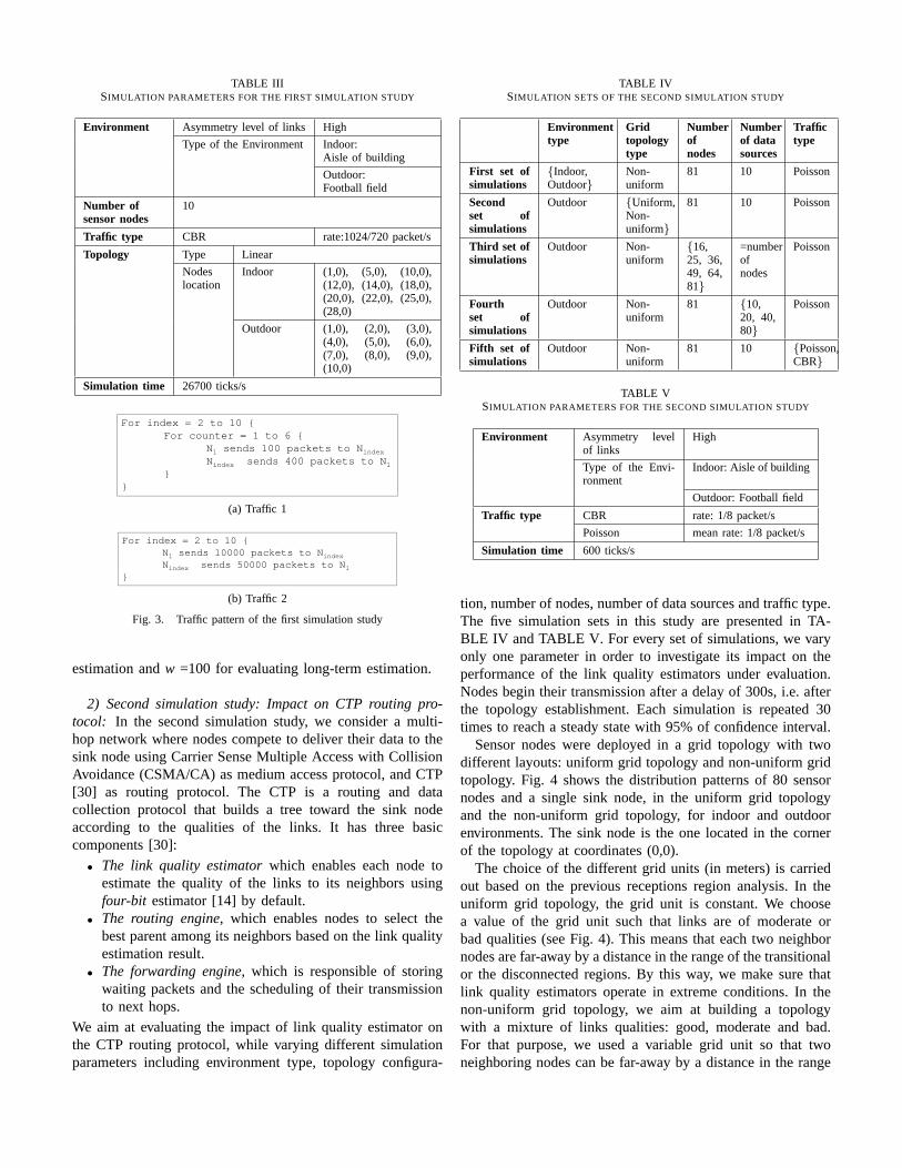
TABLE IIISIMULATION PARAMETERS FOR THE FIRST SIMULATION STUDY

Environment Asymmetry level of links High

Type of the Environment Indoor:Aisle of building

Outdoor:Football field

Number ofsensor nodes

10

Traffic type CBR rate:1024/720 packet/s

Topology Type Linear

Nodeslocation

Indoor (1,0), (5,0), (10,0),(12,0), (14,0), (18,0),(20,0), (22,0), (25,0),(28,0)

Outdoor (1,0), (2,0), (3,0),(4,0), (5,0), (6,0),(7,0), (8,0), (9,0),(10,0)

Simulation time 26700 ticks/s

For index = 2 to 10 {For counter 1 to 6 {For counter = 1 to 6 {

N1 sends 100 packets to NindexNindex sends 400 packets to N1

}}}

F i d 2 t 10 {For index = 2 to 10 {N1 sends 10000 packets to NindexNindex sends 50000 packets to N1

}}

(a) Traffic 1

For index = 2 to 10 {For counter 1 to 6 {For counter = 1 to 6 {

N1 sends 100 packets to NindexNindex sends 400 packets to N1

}}}

F i d 2 t 10 {For index = 2 to 10 {N1 sends 10000 packets to NindexNindex sends 50000 packets to N1

}}

(b) Traffic 2

Fig. 3. Traffic pattern of the first simulation study

estimation andw =100 for evaluating long-term estimation.

2) Second simulation study: Impact on CTP routing pro-tocol: In the second simulation study, we consider a multi-hop network where nodes compete to deliver their data to thesink node using Carrier Sense Multiple Access with CollisionAvoidance (CSMA/CA) as medium access protocol, and CTP[30] as routing protocol. The CTP is a routing and datacollection protocol that builds a tree toward the sink nodeaccording to the qualities of the links. It has three basiccomponents [30]:

• The link quality estimatorwhich enables each node toestimate the quality of the links to its neighbors usingfour-bit estimator [14] by default.

• The routing engine, which enables nodes to select thebest parent among its neighbors based on the link qualityestimation result.

• The forwarding engine, which is responsible of storingwaiting packets and the scheduling of their transmissionto next hops.

We aim at evaluating the impact of link quality estimator onthe CTP routing protocol, while varying different simulationparameters including environment type, topology configura-

TABLE IVSIMULATION SETS OF THE SECOND SIMULATION STUDY

Environmenttype

Gridtopologytype

Numberofnodes

Numberof datasources

Traffictype

First set ofsimulations

{Indoor,Outdoor}

Non-uniform

81 10 Poisson

Secondset ofsimulations

Outdoor {Uniform,Non-uniform}

81 10 Poisson

Third set ofsimulations

Outdoor Non-uniform

{16,25, 36,49, 64,81}

=numberofnodes

Poisson

Fourthset ofsimulations

Outdoor Non-uniform

81 {10,20, 40,80}

Poisson

Fifth set ofsimulations

Outdoor Non-uniform

81 10 {Poisson,CBR}

TABLE VSIMULATION PARAMETERS FOR THE SECOND SIMULATION STUDY

Environment Asymmetry levelof links

High

Type of the Envi-ronment

Indoor: Aisle of building

Outdoor: Football field

Traffic type CBR rate: 1/8 packet/s

Poisson mean rate: 1/8 packet/s

Simulation time 600 ticks/s

tion, number of nodes, number of data sources and traffic type.The five simulation sets in this study are presented in TA-BLE IV and TABLE V. For every set of simulations, we varyonly one parameter in order to investigate its impact on theperformance of the link quality estimators under evaluation.Nodes begin their transmission after a delay of 300s, i.e. afterthe topology establishment. Each simulation is repeated 30times to reach a steady state with 95% of confidence interval.

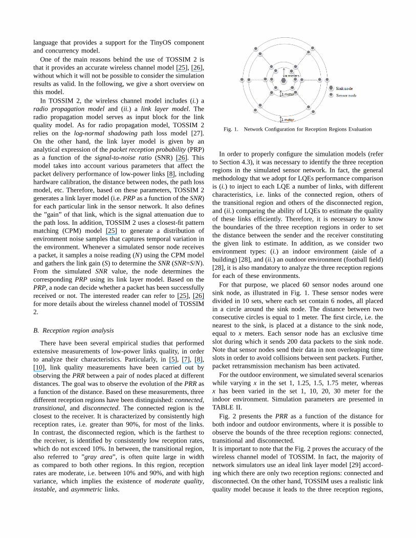
Sensor nodes were deployed in a grid topology with twodifferent layouts: uniform grid topology and non-uniform gridtopology. Fig. 4 shows the distribution patterns of 80 sensornodes and a single sink node, in the uniform grid topologyand the non-uniform grid topology, for indoor and outdoorenvironments. The sink node is the one located in the cornerof the topology at coordinates (0,0).

The choice of the different grid units (in meters) is carriedout based on the previous receptions region analysis. In theuniform grid topology, the grid unit is constant. We choosea value of the grid unit such that links are of moderate orbad qualities (see Fig. 4). This means that each two neighbornodes are far-away by a distance in the range of the transitionalor the disconnected regions. By this way, we make sure thatlink quality estimators operate in extreme conditions. In thenon-uniform grid topology, we aim at building a topologywith a mixture of links qualities: good, moderate and bad.For that purpose, we used a variable grid unit so that twoneighboring nodes can be far-away by a distance in the range

120

Uniform grid(Grid unit =14 m) 60

Non-uniform grid(Grid unit {4 m,14 m})

80

100

120

30

40

50

60

20

40

60

10

20

30

00 20 40 60 80 100 120

00 10 20 30 40 50 60 70 80

35404550

Uniform grid(Grid unit =5,5 m)

25

30

35Non-uniform grid

(Grid unit {4 m,14 m})

1520253035

10

15

20

25

05

10

0 10 20 30 40 500

5

0 5 10 15 20 25 30

(a) Indoor environment: aisle of building

120

Uniform grid(Grid unit =14 m) 60

Non-uniform grid(Grid unit {4 m,14 m})

80

100

120

30

40

50

60

20

40

60

10

20

30

00 20 40 60 80 100 120

00 10 20 30 40 50 60 70 80

35404550

Uniform grid(Grid unit =5,5 m)

25

30

35Non-uniform grid

(Grid unit {4 m,14 m})

1520253035

10

15

20

25

05

10

0 10 20 30 40 500

5

0 5 10 15 20 25 30

(b) Outdoor environment: football field

Fig. 4. Distribution pattern of 80 sensor nodes and a single sink node, inuniform and non-uniform grid topologies

of the connected, transitional or disconnected regions.Note thatfour-bit is the native estimator for CTP, thus, we haveadditionally implemented the other four link quality estimatorsin TOSSIM. We choose a history control factorα = 0.9 andaveraging windoww to 5 [14].

V. PERFORMANCEANALYSIS

In this section, we analyze the complexity and resourceusage of the estimators, and we evaluate their performancesbased on the results of both simulation scenarios, described inthe previous section.

A. First simulation study: performance of LQEs

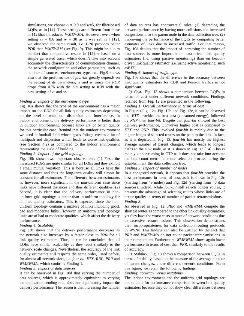
In the first scenario, we study (i.) the temporal behaviour ofLQEs, as illustrated in Fig. 5, and (ii .) the statistical propertiesof LQEs, shown in Fig. 7, Fig. 6, Fig. 8. In the statisticalanalysis of LQEs, we measured the following metrics:

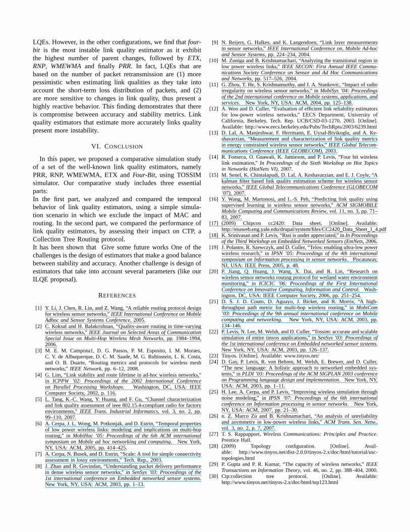
• The empirical cumulative distribution function (CDF),which assesses the level of over-estimation of each LQE,presented in Fig. 6. The over-estimation level is definedas ”how much the estimator deviate from reality byestimating the link at a certain level of goodness when itis not good as it has been estimated”. We have presentedthe results by considering all nodes of the indoor envi-ronment simulation. These results are similar to those ofthe outdoor environment.

• The coefficient of variation (CV) , which is defined as theratio of the standard deviation to the mean. It comparesthe performance of the LQEs in terms of stability. Resultsrelated to LQEs stability are presented in Fig. 7.

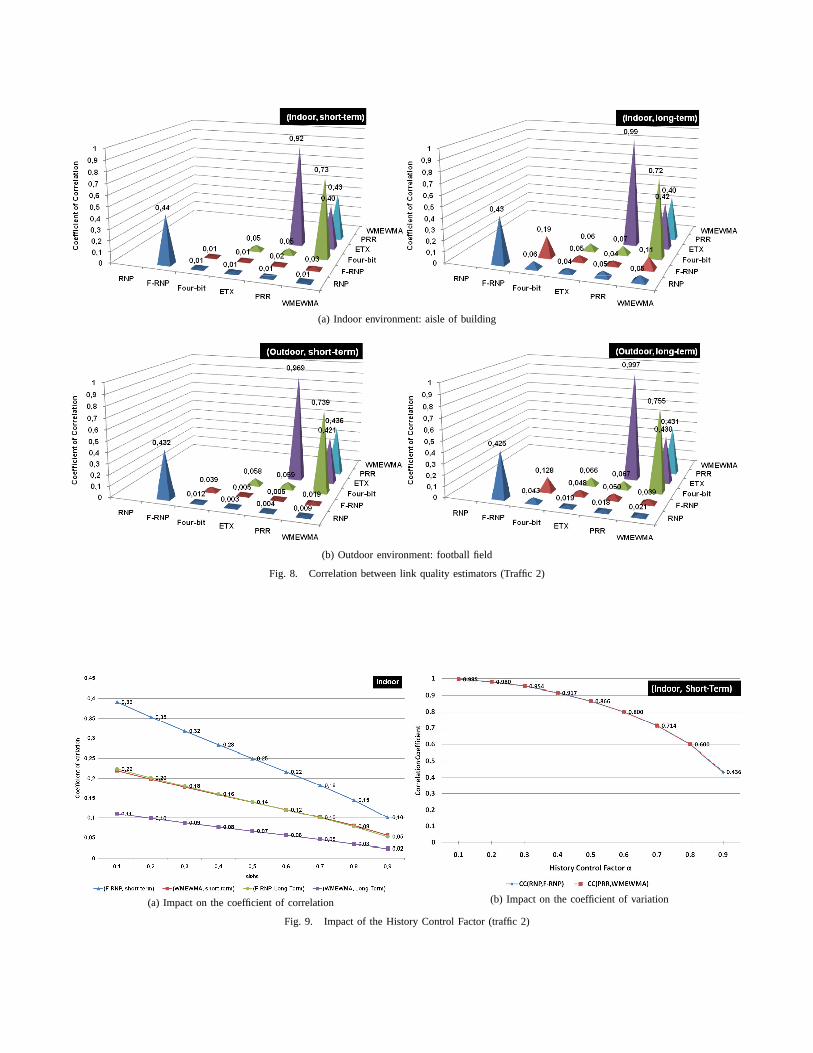
• The absolute value of the coefficient of correlation (CC),which expresses the degree of linear dependency betweena pair of Link quality estimators. Results are presentedin Fig. 8.

In what follows, we present the main lessons learnt from thefirst simulation study.

1) Over-estimation: In Fig. 6, it can be observed thatWMEWMA, PRR and ETX are the most optimistic estima-tors andRNP, F-RNP and four-bits are the least optimisticestimators. This means that thePRR-based estimators tend toover-estimate the link quality. The main reason is that thePRR-based estimators are not aware of the number of retransmittedpackets, since they are implemented at the receiver side.A packet that is lost after one retransmission or afternretransmissions will produce the samePRR-based estimate,in contrast to count-based estimates, which are quite sensitiveto retransmissions, hidden to the receiver.

This finding is clearly illustrated in Fig. 5b for the link(1←7). In fact, PRR, WMEWMAand ETX estimate the linkas continuously being at the best quality (100% of success),whereasfour-bit, RNPandF-RNPshows that the link qualityfluctuates between 0 and 7 retransmissions, which demonstratethat the link is not as good as inferred byPRR-based metrics.

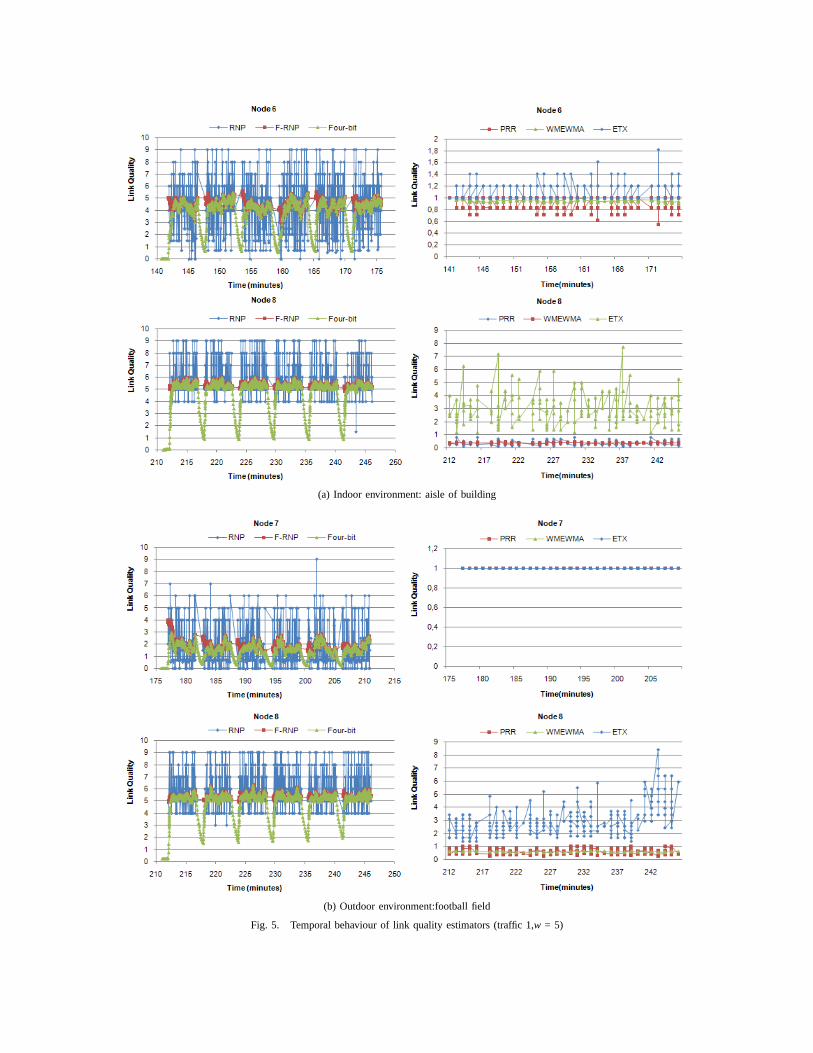
2) Stability: Fig. 7 shows the average CV for each LQEfrom all nodes for different widow sizes :w = 100 (long-termestimation) andw = 5 (short-term estimation), and differentenvironments: indoor, outdoor. Traffic 2 has been used in thissimulation.

First, according to Fig. 7, we observe thatWMEWMAandF-RNPare the most stable in general. This can also be observedthrough the temporal behavior in Fig. 5. The main reason isthat these estimators are based on filtering technique, whichsmoothes the variation of the link quality and turn themmore robust to quality fluctuations than other estimators. Inparticular, the use of a history control factorα = 0.9 increasesthe stability of those filter-based estimators. In fact, the historyfactor has an impact on the stability of filter-based estimators,as shown in Fig. 9a. It is easily observed that the coefficient ofvariation of the filter-based estimators linearly decreases as thehistory control factorα increases, which turns their behaviormore stable. In practice, it is important to adequately tune thehistory control factor to make a balance between stability andresponsiveness to link quality changes. Fig. 9aalso confirmsthat WMEWMAremains almost the most stable estimators forany value of the factor .

Second,four-bit is the least stable LQE, although it relieson two filter-based estimators. The reason is thatfour-bitcombines two different estimators that have different rangeof values (refer to Eq. (7)), as it is based on the inverse ofWMEWMA in the upstream direction and onF-RNP in thedownstream direction. Four-bit can, however, be more stable ifwe only consider Eq. (6) as the actual output of the estimatorand Eq. (5) as a corrective estimate when the downstreamtraffic is low. This can be observed in the temporal behavior inFig. 5, where thefour-bit estimates sharply decrease wheneverWMEWMAis used for each incoming packet.

Third, the study also reveals that all estimators are morestable in long-term estimation (i.e.w = 100) than in short-termestimation (i.e.w = 5), as shown in Fig. 7 and Fig. 9a. This isa reasonable result since the average estimation in long-term

will be closer to the steady state than that in short-term, whichis more prone to changes. In this particular case, by applyinga linear regression analysis on the short-term CV with theircorresponding long-term CV, we found that the long-term CVof each estimator (withw = 100) is nearly the half of its short-term CV (with w = 5). This infers a strong linear correlationbetween the short-term and long-term CV vectors.

Stability results described above are also confirmed byobserving the temporal behavior of LQEs in Fig. 5.

In conclusion, filter-based estimators are thus more stableand more robust to quality fluctuations than other estimators.

3) Correlation: Correlation analysis enables to classify theestimators into different classes with similar behavior. Basedon the results in Fig. 8, we can roughly draw the followingconclusions.

First, there is strong linear correlation betweenPRR andETX although they are computed in completely differentmanner. Note that these two metrics are not correlated withthe other estimators. The reason is

Second,RNP and F-RNP are weakly correlated, similarlyto PRRand WMEWMA. The main reason is that the controlhistory factor is too high such that the filter-based estimatorsare mostly related to the link quality history than to the currentquality. For smaller values of the correlation ofRNPandPRRestimators with their filter-based versions increases, as shownin Fig. 9b. Note that the behavior of the LQEs shown in Fig. 9bis similar to those for the outdoor environment and for long-term estimation.

Third, the correlation betweenfour-bit and F-RNP on theone hand, and betweenfour-bit and WMEWMAon the otherhand is traffic-specific. It in fact heavily depends on the pro-portion between the traffic being sent and that being received.In fact, Fig. 8 shows a strong correlation betweenfour-bitandWMEWMAwhereas the correlation betweenfour-bit andF-RNP is very weak. This is very much related to the useof traffic 2, i.e. a node receives a first bunch of packets thensends another bunch of packets. In contrast, Fig. 9b shows thatthe use of traffic 1 where sent and received packets are moreevenly distributed over time makes that four-bit is no longermuch correlated with its composite estimators. In general,four-bit would not be correlated neither toWMEWMA norto F-RNP, or in best case weakly correlated since in a realdeployment, the traffic between sensor nodes would be muchcloser to traffic 1.

B. Second simulation study: impact of LQEs on CTP routingprotocol

In the second scenario, we evaluate the impact of LQEson CTP routing protocol and we compare their performancein terms of accuracy, cost and stability, when subjected todifferent network conditions, including the environment type,the grid topology type, the network size, the number of datasources and the traffic type.

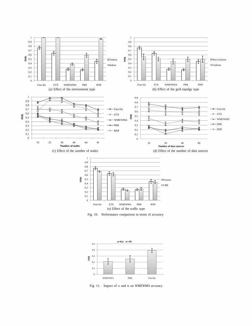
1) Accuracy: Fig. 10 shows a comparison between linkquality estimators in terms of accuracy based on the measureof the packet delivery rate (see Section 4.4) under different

network conditions. Based on this figure, we retain the fol-lowing findings.Finding1: Impact of the estimator classIn Fig. 10a to Fig. 10e, we clearly observe that thePDRs ofthe four link quality estimators are organized in the followingdecreasing accuracy order (from the most to the less accu-rate): (1) four-bit, (2) ETX, (3) RNP, (4) PRR and then (5)WMEWMA. This observation highlights three main outcomes.

• First, the accuracy offour-bit and RNP comparing toPRRandWMEWMAis justified by the fact that the firstsintegrateRNPmetric whereas the seconds integratePRRmetric. As we have shown in the previous simulationstudy, PRR-based LQEs overestimate the link qualityas they provide a coarse-grain estimation of the linkquality, in contrast toRNP-based LQEs. Nevertheless,ETX also integratesPRRmetric, yet it is more accuratethan RNP. Its accuracy is due to the fact that it relieson active monitoring. In fact, in the first simulationstudy, we have shown thatETX overestimate link qualityjust like PRR and WMEWMA. But in this study weimplementedETX with passive monitoring, instead ofactive monitoring. In this study,ETX relies on activemonitoring to derive estimate. In addition, the beaconingrate is high (1packet/s) comparing to the data traffic rate(1/8 packet/s). Consequently,ETX have frequently freshinformation on links states, which enable it to provideaccurate link quality estimate. Therefore the accuracy ofETX would be due to the active monitoring and not dueto the metric itself.

• Second,four-bit leads to slightly better delivery perfor-mance thanETX. This might be due to the fact thatfour-bit integrates a metric that count the required number ofpacket retransmissions (RNP), butETX approximates therequired number of packet retransmissions.

• Third, the accuracy offour-bit comparing toRNPcan beexplained by the following:four-bit integrates bothPRRand RNP metrics. In one handPRR have been shownto overestimate the links quality. On the other hand, weshowed also thatRNP is pessimistic. In other words, itunderestimates link quality. Therefore, the performanceof four-bit comparing toRNPcan be due to the fact thatthese LQEs integrate two metrics that enable to have abalance between overestimating and underestimating linkquality.

• Fourth, regarding LQEs that count or approximate thepacket reception rate, we found that thePRR metricleads to a slightly better delivery performance than doesWMEWMA, which means thatPRR is more accuratethan WMEWMA, in contrast to the results in [12]. Oneof the reasons is thatPRR is more reactive to qual-ity changes thanWMEWMA since the latter is filter-based. Furthermore, in [12], accuracy is not measuredby the PDR but by the mean square error between themeasured link quality and the estimated link quality(refer to related work, section 2.2). Recall that in our

simulations, we chooseα = 0.9 andw=5, for filter-basedLQEs, as in [14]. These settings are different from thosein [12]that introducedWMEWMA. However, even whensetting α = 0.6 andw = 30 as it was set in [ [12],we observed the same result, i.e.PRR provides betterPDR thanWMEWAM(see Fig. 9). This might be due tothe fact that comparative results in [12]are based on asimple generated trace, which doesn’t take into accountaccurately the characteristics of communication channel,the network configuration and other parameters, such asnumber of sources, environment type, etc. Fig.9 showsalso that the performance offour-bit greatly depends onthe setting of its parameters,α and w, since thePDRdrops from 0.76 with the old setting to 0.39 with thenew setting ofα andw.

Finding 2: Impact of the environment typeFig. 10a shows that the type of the environment has a majorimpact on thePDR for all link quality estimators dependingon the level of multipath dispersion and interference. Inindoor environment, the delivery performance is better thanin outdoor environment, because links are of better qualityfor this particular case. Remind that the outdoor environmentwe used is football field whose grass foliage creates a lot ofmultipath and dispersion which leads to worse link qualities(see Section 4.2) as compared to the indoor environmentrepresenting the aisle of building.Finding 3: Impact of the grid topologyFig. 10b shows two important observations: (1) First, themeasuredPDRsare quite similar for all LQEs and they exhibita small mutual variation. This is because all links have thesame distance and thus the long-term quality will almost beconstant for all estimators. The difference between estimatorsis, however, more significant in the non-uniform case sincelinks have different distances and thus different qualities. (2)Second, it is clear that the delivery performance in non-uniform grid topology is better than in uniform topology forall link quality estimators. This is expected since the non-uniform topology contains a mixture of links including good,bad and moderate links. However, in uniform grid topologylinks are of bad or moderate qualities, which affect the deliveryperformance.Finding 4: ScalabilityFig. 10c shows that the delivery performance decreases asthe network size increases by a factor close to 30% for alllink quality estimators. Thus, it can be concluded that allLQEs have similar scalability as they react similarly to thenetwork scale changes. Nevertheless, the accuracy of the linkquality estimators still respects the same order, listed before,for almost all network sizes, i.e.four-bit, ETX, RNP, PRRandWMEWMA, which confirms Finding 1.Finding 5: Impact of data sourcesIt can be observed in Fig. 10d that varying the number ofdata sources, which is approximately equivalent to varyingthe application sending rate, does not significantly impact thedelivery performance. The reason is that increasing the number

of data sources has controversial roles: (1) degrading thenetwork performance by having more collisions and increasedcongestions in at the parent node in the data collection tree, (2)improving the performance of the LQEs by computing betterestimates of links due to increased traffic. For that reason,Fig. 10d depicts that the impact of increasing the number ofdata sources is more important on data-driven link qualityestimators (i.e. using passive monitoring) than on beacon-driven link quality estimator (i.e. using active monitoring, suchasETX).Finding 6: impact of traffic typeFig. 10e shows that the difference in the accuracy betweenlink quality estimators for CBR and Poisson traffics is notsignificant.

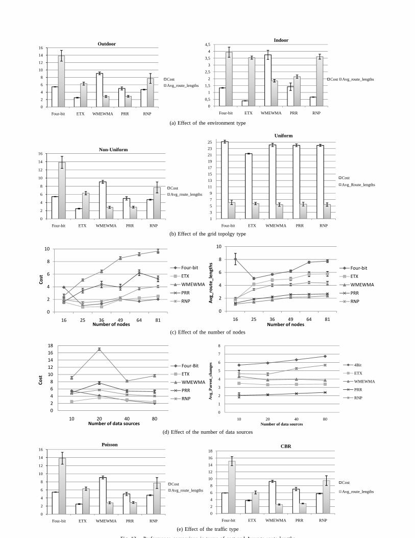
2) Cost: Fig. 12 shows a comparison between LQEs interms of cost under different network conditions. Findingsretained from Fig. 12 are presented in the following.Finding 1: Overall performance in terms of costIn Figures Fig. 12a, Fig. 12b and Fig. 12e, it can be observedthat ETX provides the best cost (consumed energy), followedby RNP then four-bit. Despite thatfour-bit showed the bestdelivery performance, it involves higher cost as compared toETX and RNP. This involved four-bit is mainly due to thehigher length of selected routes on the path to the sink. In fact,as it is depicted in Fig. 13,four-bit has mostly the highestaverage number of parent changes, which leads to longestpaths to the sink node, as it is shown in Fig. 12 [14]. This ismainly a shortcoming in CTP as it does not take into accountthe hop count metric in route selection process during theestablishment the data collection tree.Finding 2: Impact of number of nodesIn a congested network, it appears thatfour-bit provides thebest performance in terms of cost, as it is shown in Fig. 12c(starting from 49 nodes) and Fig. 12d (starting from 40 datasources). Indeed, whilefour-bit still selects longer routes, itpresents the advantage of selecting routes whose links are ofbetter quality in terms of number of packet retransmissions.Finding 3:As observed in Fig. 12,PRR and WMEWMA compute theshortest routes as compared to the other link quality estimators,yet they have the worst costs in most of network conditions dueto excessive retransmissions. This observation demonstratestheir inappropriateness for data collection routing protocolsin WSNs. This finding can also be justified by the fact thatPRRand WMEWMAdo not count packet retransmissions intheir computation. Furthermore,WMEWMAshows again lowerperformance in terms of cost thanPRR, similarly to the resultsof accuracy.

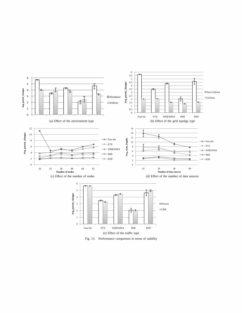
3) Stability: Fig. 13 shows a comparison between LQEs interms of stability, based on the measure of the average numberof parent changes, under different network conditions. Formthis figure, we retain the following findings.Finding: accuracy versus instabilityThe indoor environment and the uniform grid topology arenot suitable for performance comparison between link qualityestimators because they do not show clear differences between

LQEs. However, in the other configurations, we find thatfour-bit is the most instable link quality estimator as it exhibitthe highest number of parent changes, followed byETX,RNP, WMEWMA and finally PRR. In fact, LQEs that arebased on the number of packet retransmission are (1) morepessimistic when estimating link qualities as they take intoaccount the short-term loss distribution of packets, and (2)are more sensitive to changes in link quality, thus present ahighly reactive behavior. This finding demonstrates that thereis compromise between accuracy and stability metrics. Linkquality estimators that estimate more accurately links qualitypresent more instability.

VI. CONCLUSION

In this paper, we proposed a comparative simulation studyof a set of the well-known link quality estimators, namelyPRR, RNP, WMEWMA, ETX andFour-Bit, using TOSSIMsimulator. Our comparative study includes three essentialparts:In the first part, we analyzed and compared the temporalbehavior of link quality estimators, using a simple simula-tion scenario in which we exclude the impact of MAC androuting. In the second part, we compared the performance oflink quality estimators, by assessing their impact on CTP, aCollection Tree Routing protocol.It has been shown that Give some future works One of thechallenges is the design of estimators that make a good balancebetween stability and accuracy. Another challenge is design ofestimators that take into account several parameters (like ourILQE proposal).

REFERENCES

[1] Y. Li, J. Chen, R. Lin, and Z. Wang, “A reliable routing protocol designfor wireless sensor networks,”IEEE International Conference on MobileAdhoc and Sensor Systems Conference, 2005.

[2] C. Koksal and H. Balakrishnan, “Quality-aware routing in time-varyingwireless networks,”IEEE Journal on Selected Areas of CommunicationSpecial Issue on Multi-Hop Wireless Mesh Networks, pp. 1984–1994,2006.

[3] M. E. M. Campista1, D. G. Passos, P. M. Esposito, I. M. Moraes,C. V. de Albuquerque, D. C. M. Saade, M. G. Rubinstein, L. K. Costa,and O. B. Duarte, “Routing metrics and protocols for wireless meshnetworks,” IEEE Network, pp. 6–12, 2008.

[4] G. Lim, “Link stability and route lifetime in ad-hoc wireless networks,”in ICPPW ’02: Proceedings of the 2002 International Conferenceon Parallel Processing Workshops. Washington, DC, USA: IEEEComputer Society, 2002, p. 116.

[5] L. Tang, K.-C. Wang, Y. Huang, and F. Gu, “Channel characterizationand link quality assessment of ieee 802.15.4-compliant radio for factoryenvironments,”IEEE Trans. Industrial Informatics, vol. 3, no. 2, pp.99–110, 2007.

[6] A. Cerpa, J. L. Wong, M. Potkonjak, and D. Estrin, “Temporal propertiesof low power wireless links: modeling and implications on multi-hoprouting,” in MobiHoc ’05: Proceedings of the 6th ACM internationalsymposium on Mobile ad hoc networking and computing. New York,NY, USA: ACM, 2005, pp. 414–425.

[7] A. Cerpa, N. Busek, and D. Estrin, “Scale: A tool for simple connectivityassessment in lossy environments,” Tech. Rep., 2003.

[8] J. Zhao and R. Govindan, “Understanding packet delivery performancein dense wireless sensor networks,” inSenSys ’03: Proceedings of the1st international conference on Embedded networked sensor systems.New York, NY, USA: ACM, 2003, pp. 1–13.

[9] N. Reijers, G. Halkes, and K. Langendoen, “Link layer measurementsin sensor networks,”IEEE International Conference on, Mobile Ad-hocand Sensor Systems, pp. 224–234, 2004.

[10] M. Zuniga and B. Krishnamachari, “Analyzing the transitional region inlow power wireless links,”IEEE SECON: First Annual IEEE Commu-nications Society Conference on Sensor and Ad Hoc Communicationsand Networks, pp. 517–526, 2004.

[11] G. Zhou, T. He, S. Krishnamurthy, and J. A. Stankovic, “Impact of radioirregularity on wireless sensor networks,” inMobiSys ’04: Proceedingsof the 2nd international conference on Mobile systems, applications, andservices. New York, NY, USA: ACM, 2004, pp. 125–138.

[12] A. Woo and D. Culler, “Evaluation of efficient link reliability estimatorsfor low-power wireless networks,” EECS Department, University ofCalifornia, Berkeley, Tech. Rep. UCB/CSD-03-1270, 2003. [Online].Available: http://www.eecs.berkeley.edu/Pubs/TechRpts/2003/6239.html

[13] D. Lal, A. Manjeshwar, F. Herrmann, E. Uysal-Biyikoglu, and A. Ke-shavarzian, “Measurement and characterization of link quality metricsin energy constrained wireless sensor networks,”IEEE Global Telecom-munications Conference (IEEE GLOBECOM), 2003.

[14] R. Fonseca, O. Gnawali, K. Jamieson, and P. Levis, “Four bit wirelesslink estimation,” In Proceedings of the Sixth Workshop on Hot Topicsin Networks (HotNets VI), 2007.

[15] M. Senel, K. Chintalapudi, D. Lal, A. Keshavarzian, and E. J. Coyle, “Akalman filter based link quality estimation scheme for wireless sensornetworks,”IEEE Global Telecommunications Conference (GLOBECOM’07), 2007.

[16] Y. Wang, M. Martonosi, and L.-S. Peh, “Predicting link quality usingsupervised learning in wireless sensor networks,”ACM SIGMOBILEMobile Computing and Communications Review, vol. 11, no. 3, pp. 71–83, 2007.

[17] (2009) Chipcon cc2420: Data sheet. [Online]. Available:http://enaweb.eng.yale.edu/drupal/system/files/CC2420Data Sheet1 4.pdf

[18] K. Srinivasan and P. Levis, “Rssi is under appreciated,” inIn Proceedingsof the Third Workshop on Embedded Networked Sensors (EmNets, 2006.

[19] J. Polastre, R. Szewczyk, and D. Culler, “Telos: enabling ultra-low powerwireless research,” inIPSN ’05: Proceedings of the 4th internationalsymposium on Information processing in sensor networks. Piscataway,NJ, USA: IEEE Press, 2005, p. 48.

[20] P. Jiang, Q. Huang, J. Wang, X. Dai, and R. Lin, “Research onwireless sensor networks routing protocol for wetland water environmentmonitoring,” in ICICIC ’06: Proceedings of the First InternationalConference on Innovative Computing, Information and Control. Wash-ington, DC, USA: IEEE Computer Society, 2006, pp. 251–254.

[21] D. S. J. D. Couto, D. Aguayo, J. Bicket, and R. Morris, “A high-throughput path metric for multi-hop wireless routing,” inMobiCom’03: Proceedings of the 9th annual international conference on Mobilecomputing and networking. New York, NY, USA: ACM, 2003, pp.134–146.

[22] P. Levis, N. Lee, M. Welsh, and D. Culler, “Tossim: accurate and scalablesimulation of entire tinyos applications,” inSenSys ’03: Proceedings ofthe 1st international conference on Embedded networked sensor systems.New York, NY, USA: ACM, 2003, pp. 126–137.

[23] Tinyos. [Online]. Available: www.tinyos.net/[24] D. Gay, P. Levis, R. von Behren, M. Welsh, E. Brewer, and D. Culler,

“The nesc language: A holistic approach to networked embedded sys-tems,” inPLDI ’03: Proceedings of the ACM SIGPLAN 2003 conferenceon Programming language design and implementation. New York, NY,USA: ACM, 2003, pp. 1–11.

[25] H. Lee, A. Cerpa, and P. Levis, “Improving wireless simulation throughnoise modeling,” inIPSN ’07: Proceedings of the 6th internationalconference on Information processing in sensor networks. New York,NY, USA: ACM, 2007, pp. 21–30.

[26] n. Z. Marco Zu and B. Krishnamachari, “An analysis of unreliabilityand asymmetry in low-power wireless links,”ACM Trans. Sen. Netw.,vol. 3, no. 2, p. 7, 2007.

[27] T. S. Rappapport,Wireless Communications: Principles and Practice.Prentice Hall.

[28] (2009) Topology configuration. [Online]. Avail-able: http://www.tinyos.net/dist-2.0.0/tinyos-2.x/doc/html/tutorial/usc-topologies.html

[29] P. Gupta and P. R. Kumar, “The capacity of wireless networks,”IEEETransactions on Information Theory, vol. 46, no. 2, pp. 388–404, 2000.

[30] Ctp:collection tree protocol. [Online]. Available:http://www.tinyos.net/tinyos-2.x/doc/html/tep123.html

(a) Indoor environment: aisle of building

(b) Outdoor environment:football field

Fig. 5. Temporal behaviour of link quality estimators (traffic 1,w = 5)

1Empirical CDF

PRR

0 7

0.8

0.9 WMEWMA

0.5

0.6

0.7

k Q

ualit

y)

0.3

0.4F(Li

nk

0.1

0.2

0 0.1 0.2 0.3 0.4 0.5 0.6 0.7 0.8 0.9 10

Link Quality

1Empirical CDF

ETX

0 7

0.8

0.9 RNPF-RNPFour-bit

0.5

0.6

0.7

k Q

ualit

y)

0.3

0.4

F(Li

nk

0.1

0.2

0 2 4 6 8 10 12 14 160

Link Quality

Fig. 6. Empirical CDFs of link quality estimators (Traffic 1, Indoor environment,w = 5)

Fig. 7. Stability of link quality estimators (Traffic 2)

(a) Indoor environment: aisle of building

(b) Outdoor environment: football field

Fig. 8. Correlation between link quality estimators (Traffic 2)

(a) Impact on the coefficient of correlation (b) Impact on the coefficient of variation

Fig. 9. Impact of the History Control Factor (traffic 2)

0,6

0,7

0,8

0,9

1

R

0

0,1

0,2

0,3

0,4

0,5

Four-bit ETX WMEWMA PRR RNP

PDR

Oudoor

Indoor

(a) Effect of the environment type

0,6

0,7

0,8

0,9

1

0

0,1

0,2

0,3

0,4

0,5

Four-bit ETX WMEWMA PRR RNP

PDR

Non-Uniform

Uniform

(b) Effect of the grid topolgy type

0,60,70,80,9

1

R

Four-bit

ETX

00,10,20,30,40,5

16 25 36 49 64 81

PDR

Number of nodes

ETX

WMEWMA

PRR

RNP

(c) Effect of the number of nodes

0,5

0,6

0,7

0,8

0,9

DR

Four-bit

ETX

0

0,1

0,2

0,3

0,4

0,5

10 20 40 80

PD

Number of data sources

WMEWMA

PRR

RNP

(d) Effect of the number of data sources

0,6

0,7

0,8

0,9

1

R

0

0,1

0,2

0,3

0,4

0,5

Four-bit ETX WMEWMA PRR RNP

PDR

Poisson

CBR

(e) Effect of the traffic type

Fig. 10. Performance comparison in terms of accuracy

0 3

0,4

0,5

R

α=0.6 w=30

0

0,1

0,2

0,3

WMEWMA PRR Four-bit

PDR

Fig. 11. Impact ofα andw on WMEWMAaccuracy

10

12

14

16Outdoor

0

2

4

6

8

10

Four-bit ETX WMEWMA PRR RNP

CostAvg_route_lengths

3

3,5

4

4,5Indoor

0

0,5

1

1,5

2

2,5

Four-bit ETX WMEWMA PRR RNP

Cost Avg_route_lengths

(a) Effect of the environment type

10

12

14

16Non-Uniform

0

2

4

6

8

Four-bit ETX WMEWMA PRR RNP

CostAvg_route_lengths

1719212325

Uniform

13579

111315

Four-bit ETX WMEWMA PRR RNP

Cost

Avg_Route_lengths

(b) Effect of the grid topolgy type

6

8

10

t

Four‐bit

ETX

0

2

4

16 25 36 49 64 81

Cos

Number of nodes

ETX

WMEWMA

PRR

RNP

6

8

10

engths Four‐bit

ETX

0

2

4

16 25 36 49 64 81

Avg_rou

te_l

Number of nodes

ETX

WMEWMA

PRR

RNP

(c) Effect of the number of nodes

1012141618

t

Four‐Bit

ETX

0246810

10 20 40 80

Cost

Number of data sources

WMEWMA

PRR

RNP

5

6

7

8

chan

ges 4Bit

ETX

0

1

2

3

4

10 20 40 80

Avg

_Par

ent_

c

Number of data sources

WMEWMA

PRR

RNP

(d) Effect of the number of data sources

10

12

14

16Poisson

0

2

4

6

8

10

Four-bit ETX WMEWMA PRR RNP

CostAvg_route_lengths

12

14

16

18CBR

0

2

4

6

8

10

Four-bit ETX WMEWMA PRR RNP

Cost

Avg_route_lengths

(e) Effect of the traffic type

Fig. 12. Performance comparison in terms of cost and Average route lengths

nbsim ompteDenumsompteDenums Expr1001 SommeDertxc nbchgt1 2443 1669 13338 3345 486

10 nœuds 4BIT

1 2443 1669 13338 3345 4862 2364 1499 12041 2506 6043 2044 1801 14623 3142 3424 2336 1468 11405 2321 6735 2354 1229 7441 2631 5496 2443 1706 13352 2946 4497 2404 1697 14055 4202 5528 2426 1306 9687 2229 5108 2426 1306 9687 2229 5109 2394 1163 7620 1503 72510 2500 1743 13108 3460 56311 2475 1906 14826 3609 54512 2421 1898 14736 2866 52313 2448 1621 13647 4565 60914 2497 1741 14154 3337 44815 2344 1689 13947 3156 57616 2476 1854 14628 3272 51217 2546 1522 10743 9605 60418 2564 1632 13443 2432 46719 2379 1784 15426 3545 53920 2311 1915 15187 3453 54521 2388 1723 13585 3155 40621 2388 1723 13585 3155 40622 2354 1640 13086 2950 55523 1918 1426 10480 3974 55024 2260 1528 12765 2938 59525 2512 1668 12720 4047 42126 2554 1846 16111 3019 54527 2252 1391 9073 1994 66828 2545 1724 13297 3385 57928 2545 1724 13297 3385 57929 2653 2008 14712 2769 41230 2531 1478 10837 2951 612

PDR MeanHop MeanRtx MeanPchgt0,68435543 7,74974645 2,02880845 6,735

StdPrr stdHop stdRtx stdPchgt0,03046101 0,21558048 0,04526995 0,02751387

4

5

6

ges

0

1

2

3 Outdoor

Indoor

Avg_p

aren

t_chan

g

(a) Effect of the environment type

3,54

4,55

5,56

_cha

nges

00,5

11,5

22,5

3,

Four-bit ETX WMEWMA PRR RNP

Avg

_par

ent_ Non-Uniform

Uniform

(b) Effect of the grid topolgy type

8

10

12

ent_

chan

ges

Four-bit

ETX

0

2

4

6

16 25 36 49 64 81

Avg

_par

e

Number of nodes

ETX

WMEWMA

PRR

RNP

(c) Effect of the number of nodes

10

12

14

16_l

engt

hs

Four-Bit

ETX

0

2

4

6

8

10 20 40 80

Avg

_rou

te_

Number of data sources

ETX

WMEWMA

PRR

RNP

(d) Effect of the number of data sources

4

5

6

_cha

nges

0

1

2

3

Four-bit ETX WMEWMA PRR RNP

Avg

_par

ent_ Poisson

CBR

(e) Effect of the traffic type

Fig. 13. Performance comparison in terms of stability