A compact fixpoint semantics for term rewriting systems

A Compact Fixpoint Semantics

for Term Rewriting Systems∗

M. Alpuente† M. Comini‡ S. Escobar† M. Falaschi§

J. Iborra†

June 2, 2010

Abstract

This work is motivated by the fact that a “compact” semantics forterm rewriting systems, which is essential for the development of effec-tive semantics-based program manipulation tools (e.g. automatic pro-gram analyzers and debuggers), does not exist. The big-step rewritingsemantics that is most commonly considered in functional program-ming is the set of values/normal forms that the program is able tocompute for any input expression. Such a big-step semantics is unnec-essarily oversized, as it contains many “semantically useless” elementsthat can be retrieved from a smaller set of terms. Therefore, in thisarticle, we present a compressed, goal-independent collecting fixpointsemantics that contains the smallest set of terms that are sufficient todescribe, by semantic closure, all possible rewritings. We prove sound-ness and completeness under ascertained conditions. The compactnessof the semantics makes it suitable for applications. Actually, our se-mantics can be finite whereas the big-step semantics is generally not,and even when both semantics are infinite, the fixpoint computationof our semantics produces fewer elements at each step. To support thisclaim we report several experiments performed with a prototypical im-plementation.

∗This work has been partially supported by the EU (FEDER), by the SpanishMEC/MICINN, under grant TIN 2007-68093-C02, and by the Italian MUR under grantRBIN04M8S8, FIRB project, Internationalization 2004.

†Departamento de Sistemas Informaticos y Computacion. Techni-cal University of Valencia, Camino de Vera s/n, 46022 Valencia, Spain.alpuente,sescobar,[email protected]

‡Dipartimento di Matematica e Informatica. University of Udine, Via delle Scienze206, 33100 Udine, Italy. [email protected]

§Dipartimento di Scienze Matematiche e Informatiche. Pian dei Mantellini 44, 53100Siena, Italy. [email protected]

1 Introduction

1.1 Why a new semantics

Finding program bugs is a long-standing problem in software construction.Unfortunately, the debugging support is rather poor for functional languages(see [40, 25, 31] and references therein), and there are no good general–purpose semantics-based debuggers available. One of the basic reasons forthe lack of simple, handy development tools for functional programs (likeprogram analyzers, debuggers, and correctors) is the lack of a suitable se-mantics that is compact and goal-independent, i.e., a program semanticsdefined only by determining the operational behavior of a small set of termsthat are sufficient to describe, by semantic closure, the meaning of all in-put expressions. The idea of such a semantics seems clear-cut, as alreadydemonstrated by several works in other programming paradigms like logicprogramming [8, 18]; however, to the best of our knowledge, it has neverbeen investigated in the context of functional programming and term rewrit-ing systems. Furthermore, the definition of such a semantics is not trivial,since we want the semantics to ensure interesting computational propertieswhile still dealing with a broad class of TRSs.

We came up with the idea of a compressed semantics when investigatingon how to convey to functional programming the semantics-based, debuggingapproach of [11, 12], for logic programs, which essentially consists of theapplication of Abstract Interpretation techniques [15] to an “appropriate”goal-independent fixpoint semantics. Among other valuable facilities, thisdebugging approach supports the development of cogent diagnostic toolsthat find program errors without having to determine symptoms in advance.The key issue of this approach is the goal-independence of the concretesemantics, meaning that the semantics is defined by collecting the observableproperties starting with “most general” calls (goals1), while still providinga complete characterization of the program behavior.

Defining a collecting semantics is usually the first crucial step in adaptingthe general methodology of Abstract Interpretation to the semantic frame-work of the programming language at hand [36]. In [1], we developed a(preliminary) Abstract Diagnosis framework for functional languages by us-ing the formalism of Term Rewriting Systems (TRSs), which is widely rec-ognized [5, 10, 28, 38] as a suitable computational model for functionalprogramming languages (e.g. Haskell, Hope, Miranda, or Maude). We useda collecting semantics that is very similar to the big-step rewriting seman-tics as a basis for the abstract debugger. However, the resulting tool wasinefficient. Not surprisingly, the main reason for this inefficiency was the ac-cidental high redundancy of the semantics, which caused the algorithms to

1Following the terminology of logic programming, we often refer to an input expression(i.e., a program call) as “the goal”.

2

use and produce redundant information at each stage. In the best case, thisredundant information reduces the performance and, in the worst case, endsin ineffective methods. In contrast, the same methodology gave good resultsin [12] because it was applied to a compact semantics (i.e., the s-semantics).

Thus, our specific objective in this paper is to avoid all such redundantelements in the semantics while still characterizing the meaning of any ex-pression. We improve previous attempts by some of the authors [4, 1] toproduce a compact, goal-independent semantics for functional programs.

1.2 Denotations as syntactic objects

Term rewriting systems [16, 28] provide an adequate computational modelfor functional languages. A functional program is a set of functions thatis defined by (oriented) equations or rules. A functional computation con-sists of replacing subexpressions by equal subexpressions (w.r.t. the functiondefinitions) until no more replacements (or reductions) are possible, and aresult is obtained.

In the literature of TRSs, equations t = s over terms t, s (with variables)are sometimes used to represent program semantics, i.e., the computed in-put/output relation of all functions. In this paper, we prefer to use (specialcases of) oriented equations t 7→ s (modulo renaming) to make explicitthe (semantic) fact that a term t reduces to term s (in symbols, t →∗ s)and not vice versa. Moreover, the equation notation is more suited in thecase of confluent TRSs. However, several of our results in this paper donot require confluence or other properties that are often assumed in tra-ditional rewriting-based languages. Modern functional languages such asMaude [10], and functional-logic languages such as Curry [23], or TOY [30]deal with non-determinism, and thus the confluence requirement is doneaway with. We also prefer t 7→ s instead of t → s to avoid confusion withprogram rules, as t 7→ s can indeed represent several reduction steps withprogram rules of the form t → s.

The idea of using syntactic domains for describing program semantics,and in particular the use of rules in the denotation, is inspired from the lit-erature of logic programming (see [8]) where it is commonly used to capturevarious computational aspects (like computed answers, call patterns, resul-tants) in a goal-independent way. For instance, the Ω-semantics of Bossi etal. [8] collects sets of Horn clauses, which model the program resultants, sothat goals can be solved by simply “executing them in the semantics”. It isimportant to note that this is generally far cheaper than executing goals inthe original program, since the “real computation” is pretty much embeddedin the representation.

Following the Ω-semantics approach, sometimes we will use the elementst 7→ s in the denotation as standard rewrite rules t → s (obviously this doesnot imply that these rules belong to the original program), and vice versa.

3

1.3 The standard big-step rewriting semantics

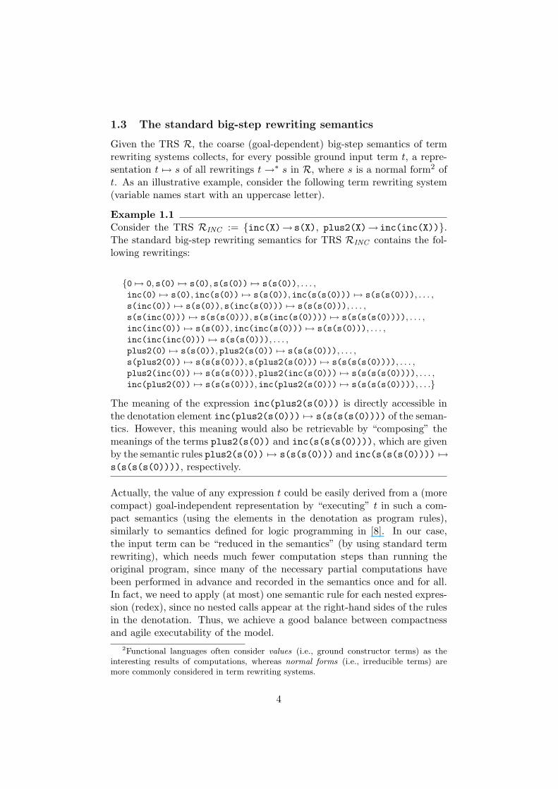
Given the TRS R, the coarse (goal-dependent) big-step semantics of termrewriting systems collects, for every possible ground input term t, a repre-sentation t 7→ s of all rewritings t →∗ s in R, where s is a normal form2 oft. As an illustrative example, consider the following term rewriting system(variable names start with an uppercase letter).

Example 1.1Consider the TRS RINC := inc(X)→ s(X), plus2(X)→ inc(inc(X)).The standard big-step rewriting semantics for TRS RINC contains the fol-lowing rewritings:

0 7→ 0, s(0) 7→ s(0), s(s(0)) 7→ s(s(0)), . . . ,inc(0) 7→ s(0), inc(s(0)) 7→ s(s(0)), inc(s(s(0))) 7→ s(s(s(0))), . . . ,s(inc(0)) 7→ s(s(0)), s(inc(s(0))) 7→ s(s(s(0))), . . . ,s(s(inc(0))) 7→ s(s(s(0))), s(s(inc(s(0)))) 7→ s(s(s(s(0)))), . . . ,inc(inc(0)) 7→ s(s(0)), inc(inc(s(0))) 7→ s(s(s(0))), . . . ,inc(inc(inc(0))) 7→ s(s(s(0))), . . . ,plus2(0) 7→ s(s(0)), plus2(s(0)) 7→ s(s(s(0))), . . . ,s(plus2(0)) 7→ s(s(s(0))), s(plus2(s(0))) 7→ s(s(s(s(0)))), . . . ,plus2(inc(0)) 7→ s(s(s(0))), plus2(inc(s(0))) 7→ s(s(s(s(0)))), . . . ,inc(plus2(0)) 7→ s(s(s(0))), inc(plus2(s(0))) 7→ s(s(s(s(0)))), . . .

The meaning of the expression inc(plus2(s(0))) is directly accessible inthe denotation element inc(plus2(s(0))) 7→ s(s(s(s(0)))) of the seman-tics. However, this meaning would also be retrievable by “composing” themeanings of the terms plus2(s(0)) and inc(s(s(s(0)))), which are givenby the semantic rules plus2(s(0)) 7→ s(s(s(0))) and inc(s(s(s(0)))) 7→s(s(s(s(0)))), respectively.

Actually, the value of any expression t could be easily derived from a (morecompact) goal-independent representation by “executing” t in such a com-pact semantics (using the elements in the denotation as program rules),similarly to semantics defined for logic programming in [8]. In our case,the input term can be “reduced in the semantics” (by using standard termrewriting), which needs much fewer computation steps than running theoriginal program, since many of the necessary partial computations havebeen performed in advance and recorded in the semantics once and for all.In fact, we need to apply (at most) one semantic rule for each nested expres-sion (redex), since no nested calls appear at the right-hand sides of the rulesin the denotation. Thus, we achieve a good balance between compactnessand agile executability of the model.

2Functional languages often consider values (i.e., ground constructor terms) as theinteresting results of computations, whereas normal forms (i.e., irreducible terms) aremore commonly considered in term rewriting systems.

4

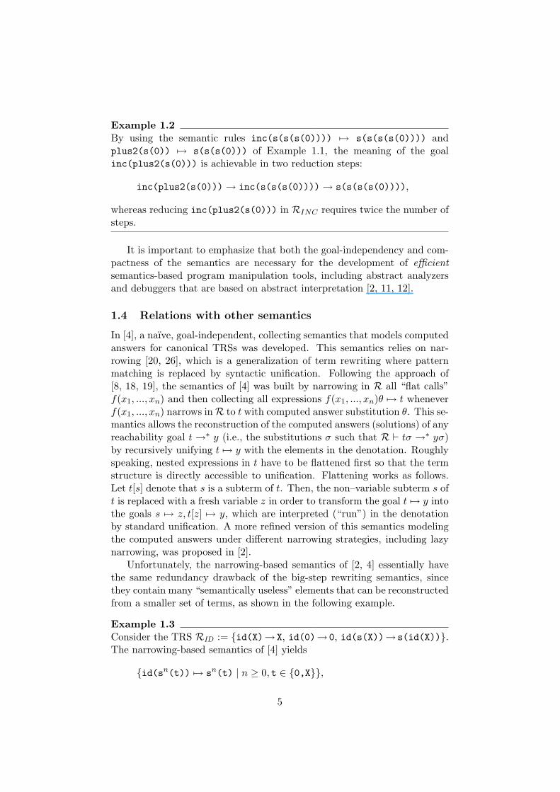
Example 1.2By using the semantic rules inc(s(s(s(0)))) 7→ s(s(s(s(0)))) andplus2(s(0)) 7→ s(s(s(0))) of Example 1.1, the meaning of the goalinc(plus2(s(0))) is achievable in two reduction steps:

inc(plus2(s(0)))→ inc(s(s(s(0))))→ s(s(s(s(0)))),

whereas reducing inc(plus2(s(0))) in RINC requires twice the number ofsteps.

It is important to emphasize that both the goal-independency and com-pactness of the semantics are necessary for the development of efficientsemantics-based program manipulation tools, including abstract analyzersand debuggers that are based on abstract interpretation [2, 11, 12].

1.4 Relations with other semantics

In [4], a naıve, goal-independent, collecting semantics that models computedanswers for canonical TRSs was developed. This semantics relies on nar-rowing [20, 26], which is a generalization of term rewriting where patternmatching is replaced by syntactic unification. Following the approach of[8, 18, 19], the semantics of [4] was built by narrowing in R all “flat calls”f(x1, ..., xn) and then collecting all expressions f(x1, ..., xn)θ 7→ t wheneverf(x1, ..., xn) narrows inR to t with computed answer substitution θ. This se-mantics allows the reconstruction of the computed answers (solutions) of anyreachability goal t →∗ y (i.e., the substitutions σ such that R ` tσ →∗ yσ)by recursively unifying t 7→ y with the elements in the denotation. Roughlyspeaking, nested expressions in t have to be flattened first so that the termstructure is directly accessible to unification. Flattening works as follows.Let t[s] denote that s is a subterm of t. Then, the non–variable subterm s oft is replaced with a fresh variable z in order to transform the goal t 7→ y intothe goals s 7→ z, t[z] 7→ y, which are interpreted (“run”) in the denotationby standard unification. A more refined version of this semantics modelingthe computed answers under different narrowing strategies, including lazynarrowing, was proposed in [2].

Unfortunately, the narrowing-based semantics of [2, 4] essentially havethe same redundancy drawback of the big-step rewriting semantics, sincethey contain many “semantically useless” elements that can be reconstructedfrom a smaller set of terms, as shown in the following example.

Example 1.3Consider the TRS RID := id(X)→ X, id(0)→ 0, id(s(X))→ s(id(X)).The narrowing-based semantics of [4] yields

id(sn(t)) 7→ sn(t) | n ≥ 0, t ∈ 0,X,

5

instead of the much more compact, accomplishable representation id(X) 7→X, which still allows the (value or normal form) meaning of any ground inputexpression to be retrieved by standard rewriting.

Nevertheless, it is important to note that the (apparent) redundancy inthe narrowing-based semantics of [2, 4] is the key point in modeling theobservable of computed answers. For instance, in the original program,the expression id(Z) narrows to 0 with computed answer Z/0. This isperfectly captured by the semantics of [4] illustrated above, whereas it couldnot be inferred from the more “compact semantics” just containing id(X) 7→X. However, the exuberance in the semantics of [4] is not interesting oradmissible for the purposes of this paper, which is modeling the (value ornormal form) meaning of every expression in a pure functional language thatcan be given a rewriting semantics such as Maude [10] or Haskell [38]. Inthis paper, we are not interested in modeling computed answers.

To manifest tangibly the degree of compactness of our semantics, wepresent the experimental results obtained by a proof–of–concept implemen-tation. The benchmarks show that our compact semantics is a suitable basisfor the development of efficient automatic program analyzers and debuggers.

Plan of the paper The paper is organized as follows. We present somepreliminary notions in Section 2. In Section 3, we introduce a compressionmechanism that is based on the removal of every element that is a “rewrit-ing consequence” of other elements in the semantics. In other words, thecompact semantics is obtained by collecting only a representative set of the“most general” rewriting sequences. In order to support fixpoint compu-tations, an effective “decompression” mechanism is also formalized, whichis able to retrieve the original semantics from the compact one when it isneeded (e.g. for membership test). In Section 4, we associate a (continuous)immediate consequence operator TBT,R to a program R that allows us to de-rive the compact semantics. Similarly to [1, 4], the immediate consequenceoperator TBT,R is computed by narrowing, which provides the most generalrewriting sequences, and we ascertain the conditions that ensure that theoperator is effectively computable. Then, we prove the soundness and com-pleteness of our semantics w.r.t. the natural big-step rewriting semanticsfor some particular classes of TRSs. In Section 5 we present a prototypicalimplementation of a tool that computes (finite approximations of) the com-pressed semantics, together with some experimental evaluations. Finally,Section 6 concludes.

6

2 Preliminaries

Let us briefly recall some known results about rewrite systems [5, 39].Throughout this paper, V denotes a countably infinite set of variables andΣ denotes a finite set of function symbols, or signature, each of which has afixed associated arity. T (Σ,V) and T (Σ) denote the non-ground and groundterm algebra built on Σ ∪ V and Σ, respectively. Terms T (Σ,V) are viewedas labelled trees in the usual way. Positions are represented by sequencesof natural numbers denoting an access path in a term. The top or rootposition is denoted by ε. Given S ⊆ Σ ∪ V, OS(t) denotes the set of posi-tions of a term t that are rooted by symbols or variables in S. Of(t) withf ∈ Σ ∪ V is simply denoted by Of (t). t|p is the subterm at the positionp of t. t[s]p is the term t with the subterm at the position p replaced withterm s. Syntactic equality of two terms t and s is represented by t = s. ByVar(s), we denote the set of variables occurring in the syntactic object s.A fresh variable is a variable that appears nowhere else. A linear term is aterm where every variable occurs only once.

A substitution is a mapping from the set of variables V into the setof terms T (Σ,V), which differs from the identity only for a finite set ofvariables. A substitution is represented as x1/t1, . . . , xn/tn for variablesx1, . . . , xn and terms t1, . . . , tn. The empty substitution is denoted by id. Theapplication of substitution θ to term t is denoted by tθ. The composition ofsubstitutions θ and σ, denoted by θσ, satisfies t(θσ) = (tθ)σ. A substitutionθ is more general than σ, denoted by θ ≤ σ, if σ = θγ for some substitutionγ. We write θ|s to denote the restriction of the substitution θ to the setof variables in the syntactic object s. A renaming is a substitution σ forwhich there exists the inverse σ−1, such that σσ−1 = σ−1σ = id. A unifierof terms s and t is a substitution ϑ such that sϑ = tϑ. The most generalunifier of terms s and t, denoted by mgu(s, t), is a unifier θ such that foreach other unifier θ′, θ ≤ θ′.

A term rewriting system R (TRS for short) is a pair (Σ, R), where R isa finite set of reduction (or rewrite) rule schemes of the form l → r suchthat l, r ∈ T (Σ,V), l 6∈ V, and Var(r) ⊆ Var(l). We will often write justR instead of (Σ, R). For TRS R, l → r << R denotes that l → r is a newvariant of a rule in R such that l → r contains only fresh variables, i.e., itcontains no variable previously met during any computation (standardizedapart). We say that a TRS R is left–linear (right–linear) if the left–hand(right–hand) side of any rule l → r ∈ R is a linear term. We say that theTRS R is linear if it is left and right–linear.

A TRS R is called topmost if, for every term t, all rewritings on t are per-formed at the root position of t. Although topmost TRSs are not commonlyused in term rewriting, they are relevant in programming languages. Forinstance, in Haskell [37] or Maude [10], rewrite rules can be defined so thatthe type (or sort) information forces rewrites to happen only at the top of

7

terms. In Maude, it is also possible to introduce freezing specifications thatblock rewrites at any proper subterm position. Actually, many concurrentsystems of interest, including the vast majority of distributed algorithms,admit quite natural topmost specifications [33]. In an unsorted setting likeours, topmost TRSs are only those that do not contain any function symbolwhose arity is greater than 0 (that is, all rules have the form a → b).

Given a TRS R = (Σ, R), we assume that the signature Σ is partitionedinto two disjoint sets D := f | f(t1, . . . , tn) → r ∈ R and C := Σ \ D.Symbols in C are called constructors and symbols in D are called definedsymbols or functions. The elements of T (C,V) are called constructor terms.A pattern is a term of the form f(d1, . . . , dk) where f ∈ D and d1, . . . , dk

are constructor terms. We say that a TRS is a constructor term rewritingsystem (CS for short) if the left–hand sides of R are patterns.

A rewrite step is the application of a rewrite rule to an expression. Aterm s ∈ T (Σ,V) rewrites to a term t ∈ T (Σ,V), denoted by s →R t, ifthere exist p ∈ OΣ(s), l → r << R, and substitution σ such that s|p = lσ andt = s[rσ]p. When we want to emphasize the position p where a rewritingstep has taken place, we write s

p→R t. When we want to emphasize thatthe position q where a rewriting step has taken place is greater than someposition p, we write s

>p→R t.For substitutions σ, ρ and a set of variables V , we define σ|V → ρ|V if

there is x ∈ V such that xσ → xρ and for all other y ∈ V we have yσ = yρ.A term s is a normal form w.r.t. R (or simply a normal form), if there is

no term t such that s →R t. We denote the transitive and reflexive closure of→R by →∗

R. We write s →!R t whenever s →∗

R t with t being a normal form.A TRS R is terminating (also called strongly normalizing or noetherian) ifthere are no infinite reduction sequences t1 →R t2 →R . . . In other words,every reduction sequence eventually ends in a normal form. A TRS R isconfluent if, whenever t →∗

R s1 and t →∗R s2, there exists a term w s.t.

s1 →∗R w and s2 →∗

R w. A substitution σ is normalized if, for each x ∈ V,xσ is a normal form.

Two (possibly renamed) rules l → r and l′ → r′ overlap, if there is a non-variable position p ∈ OΣ(l) and a most-general unifier σ such that l|pσ = l′σ.The pair 〈(l[r′]p)σ, rσ〉 is called a critical pair and is also called an overlayif p = ε. A critical pair 〈t, s〉 is trivial if t = s. A left-linear TRS withoutcritical pairs is called orthogonal. A left-linear TRS where its critical pairsare trivial overlays is called almost orthogonal. Note that orthogonality andalmost orthogonality of a TRS R implies confluence of →R.

Given a TRS R = (Σ, R), the set of normal forms of R is denoted bynfR, and the set of constructor terms (or values) of R is denoted by evalR.Membership in any of these two sets is decidable. When no confusion canarise, we omit the subscript R. A different but also relevant set of termsis the set of all possible reducts of R, which is denoted by redR = s ∈

8

T (Σ,V) | t ∈ T (Σ,V), t →∗R s. Membership in redR is also decidable.

In this paper, we are also interested in rigid normal forms [3].

2.1 Narrowing and Rigid Normal Forms

Narrowing is a generalization of term rewriting that allows free variables interms (as in logic programming). In contrast to term rewriting, the left-hand side of a rule is unified with the subterm under evaluation in orderto (non-deterministically) reduce this term. Narrowing was originally intro-duced as a mechanism for solving equational unification problems [20] andthen generalized to solve the more general problem of symbolic reachability[33]. Since narrowing subsumes both rewriting and SLD-resolution, it iscomplete in the sense of functional programming (computation of normalforms) as well as logic programming (computation of answers); see [22, 23]for a survey. That is, under appropriate conditions, narrowing is able tofind “more general” solutions for the variables of terms s and t, such that srewrites to t in R in a number of steps.

Formally, a term s ∈ T (Σ,V) narrows to t ∈ T (Σ,V), denoted bys ;θ,R t (or simply s ;θ t) if there exist p ∈ OΣ(s), l → r << R, andsubstitution θ such that θ = mgu(s|p, l) and t = s[r]pθ. When we want toemphasize the position p where a narrowing step has taken place, we writes

p;θ,R t (or simply s

p;θ t). A narrowing derivation for t in R with a (par-

tially computed) answer substitution θ is defined by t ;∗θ,R t′ iff ∃θ1, . . . , θn

s.t. t ;θ1 . . . ;θn t′ and θ = (θ1 · · · θn)|t. We say that the derivation haslength n.

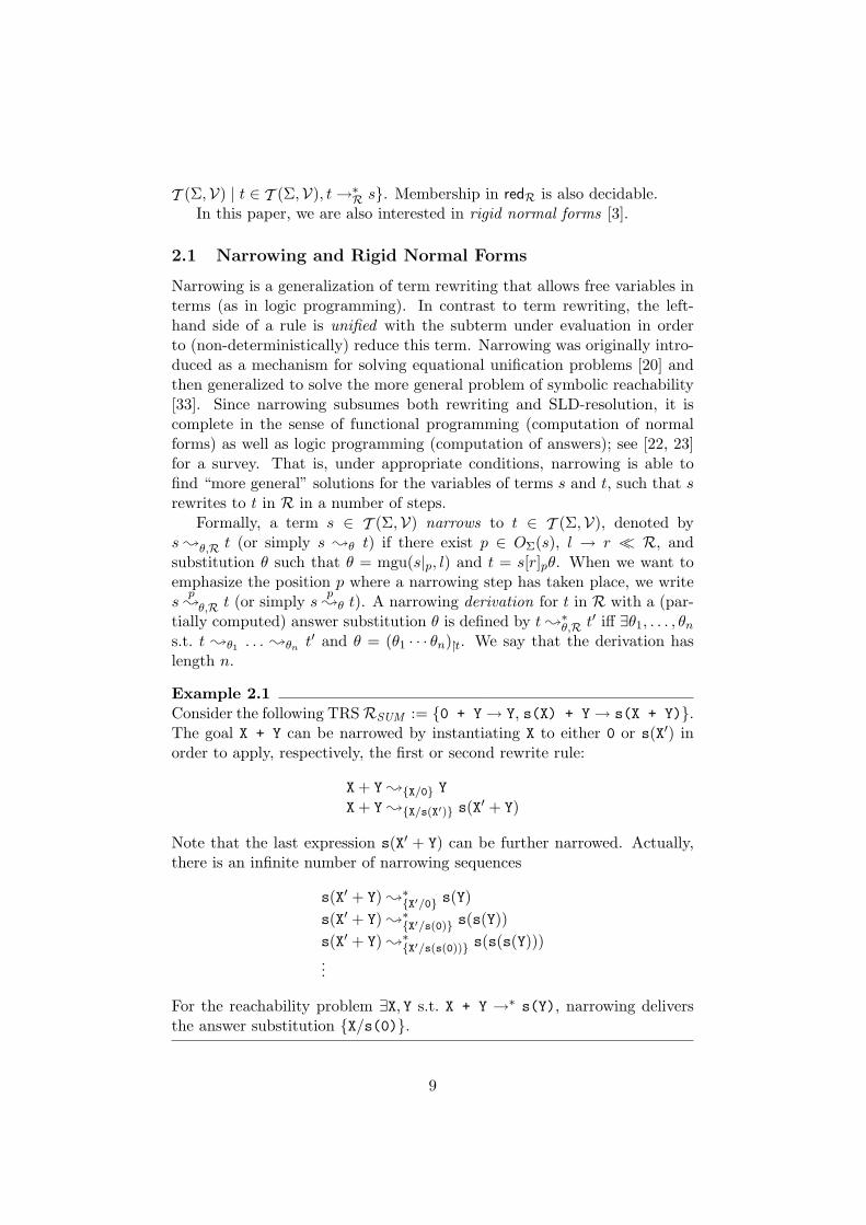
Example 2.1Consider the following TRSRSUM := 0 + Y→ Y, s(X) + Y→ s(X + Y).The goal X + Y can be narrowed by instantiating X to either 0 or s(X′) inorder to apply, respectively, the first or second rewrite rule:

X + Y ;X/0 YX + Y ;X/s(X′) s(X′ + Y)

Note that the last expression s(X′ + Y) can be further narrowed. Actually,there is an infinite number of narrowing sequences

s(X′ + Y) ;∗X′/0 s(Y)

s(X′ + Y) ;∗X′/s(0) s(s(Y))

s(X′ + Y) ;∗X′/s(s(0)) s(s(s(Y)))

...

For the reachability problem ∃X, Y s.t. X + Y →∗ s(Y), narrowing deliversthe answer substitution X/s(0).

9

Strong reachability–completeness of narrowing (i.e., completeness w.r.t.not necessarily normalized solutions) means that for every solution to areachability goal, a more general solution (modulo R) is computed by nar-rowing. In the reachability setting, where confluence cannot be assumed,this means that, for each pair t, t′ ∈ T (Σ,V) and substitution ρ such thattρ →∗

R t′, there are substitutions η, ρ′, θ and a term t′′ ∈ T (Σ,V) such thatt ;∗

η,R t′′, ρ|t →∗R ρ′, ρ′ = (ηθ)|t, and t′ = t′′θ. In other words, there is a

reduct ρ′ of solution ρ such that ρ′ is a (syntactic) instance of the substitu-tion η computed by narrowing. In [33], strong reachability–completeness isproved to hold only in particular classes of TRS:

1. topmost TRSs and2. right–linear TRSs (restricted to linear input terms).

The terminology “complete TRSs” is used in [27, 29, 34] to refer to thewell-known class of TRSs where narrowing is complete as a procedure forsolving equations (namely the class of confluent and terminating TRSs).The following definition adapts this idea to the reachability setting.

Definition 2.2 (Reachability–complete TRS) A TRS R is reachabil-ity–complete iff narrowing is strongly reachability–complete for R.

Let us now introduce the notion of rigid normal form (rnf), which isthe most important ingredient in Section 4.2.3 for effectively computinga compact semantics by deploying narrowing computations. Actually, wewill only collect in the denotation semantic rules whose right-hand sides(RHSs) are rigid normal forms, since narrowing terminates for wide classesof TRSs where the RHSs of the rewrite rules satisfy this condition (see [3]and Corollary 4.9 below).

Definition 2.3 (Rigid normal form [3]) Given a TRS R = (Σ, R), aterm s is a rigid normal form (rnf) if there is no substitution θ and positionp such that s

p;θ,R t.

Note that the notion of rigid normal form (rnf) is stronger than thestandard notion of (rewriting) normal form but can still be easily decidedby simply checking that no subterm of the considered term unifies with theleft-hand side (LHS) of any rule in R.

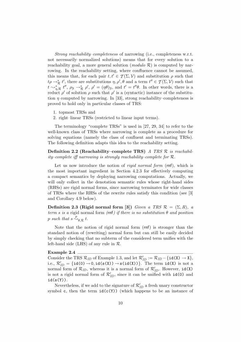
Example 2.4Consider the TRS RID of Example 1.3, and let R′

ID := RID −id(X)→ X,i.e., R′

ID = id(0)→ 0, id(s(X))→ s(id(X)). The term id(X) is not anormal form of RID , whereas it is a normal form of R′

ID . However, id(X)is not a rigid normal form of R′

ID , since it can be unified with id(0) andid(s(Y)).

Nevertheless, if we add to the signature of R′ID a fresh unary constructor

symbol c, then the term id(c(Y)) (which happens to be an instance of

10

id(X)) is a normal form as well as a rigid normal form.

The set of rigid normal forms of R is denoted by rnfR. Actually, evalR ⊆rnfR ⊆ nfR ⊆ redR. Note that when we restrict ourselves to ground terms,normal and rigid normal forms coincide, i.e., nfR ∩ T (Σ) = rnfR ∩ T (Σ).

3 A compact, goal-independent rewriting seman-tics

A compact rewriting semantics that is goal-independent should ideally in-clude only semantic rules for expressions rooted by a “defined” symbol and“relevant” arguments. Essentially, our semantics is based on the idea ofcollecting only those (unfolded) rules that are not a rewriting consequenceof other elements in the semantics; in other words, the compact semanticsis obtained by collecting only a representative set of the “most general”rewriting sequences. As in the Ω–semantics of [8] and the narrowing–basedcomputed answers semantics of [4] recalled above, we need to introducevariables in the denotation instead of collecting the meaning of ground ex-pressions. This allows us to see the semantics (when it might be convenient)as a “more efficient program” where it is still possible to run any inputexpression.

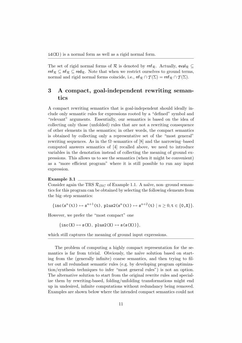
Example 3.1Consider again the TRS RINC of Example 1.1. A naıve, non–ground seman-tics for this program can be obtained by selecting the following elements fromthe big–step semantics:

inc(sn(t)) 7→ sn+1(t), plus2(sn(t)) 7→ sn+2(t) | n ≥ 0, t ∈ 0,X.

However, we prefer the “most compact” one

inc(X) 7→ s(X), plus2(X) 7→ s(s(X)),

which still captures the meaning of ground input expressions.

The problem of computing a highly compact representation for the se-mantics is far from trivial. Obviously, the naıve solution based on start-ing from the (generally infinite) coarse semantics, and then trying to fil-ter out all redundant semantic rules (e.g. by developing program optimiza-tion/synthesis techniques to infer “most general rules”) is not an option.The alternative solution to start from the original rewrite rules and special-ize them by rewriting-based, folding/unfolding transformations might endup in undesired, infinite computations without redundancy being removed.Examples are shown below where the intended compact semantics could not

11

be obtained by using this methodology. In the following, we effectively de-fine a suitable compact semantics for TRSs in the fixpoint style. Unlike thebig-step semantics, ours is truly “goal-independent”.

3.1 Rewriting Consequences

Given a signature Σ, we denote by WΣ the set of all possible semanticrules (up to renaming) built with the elements of Σ, i.e., WΣ = t 7→ s |t, s ∈ T (Σ,V)/≡ where ≡ is the variance relation extended to semanticrules, i.e., (t 7→ s) ≡ (t′ 7→ s′) iff there exists a renaming substitution ρ s.t.(t 7→ s)ρ = t′ 7→ s′. We simply write W when no confusion about Σ canarise.

In the following, any I ⊆ W is implicitly considered as an arbitraryset of semantic rules obtained by choosing an arbitrary representative ofthe elements of I in the equivalence class generated by ≡. Actually, in thefollowing, all the operators that we use on W are also independent of thechoice of the representative. Therefore, we can define any operator on W interms of its counterpart defined on sets of semantic rules, and denote thecorresponding operators by the same name.

In order to be as general as possible, we will use a family of reference(ground) big-step rewriting semantics for a TRS R, parametric on a setBT of terms known as blocking terms, where BT ∈ evalR, rnfR, nfR, redR.They model different (relevant) “rewriting behaviors” (often also called ob-servable properties) which are properties that can be observed in the com-putation space (behavior) of R. Our goal is to define suitable families of(compressed) goal-independent semantics that are correct w.r.t. these be-haviors.

Definition 3.2 (Ground big-step behaviour) Given a TRS R and aset BT of blocking terms, the ground big-step semantics BBT (R) of R w.r.t.BT is

BBT (R) := s 7→ t ∈ W | s ∈ T (Σ), s →∗R t, t ∈ BT. (3.1)

Note that Beval(R) ⊆ Brnf(R) = Bnf(R) ⊆ Bred(R).

In the case of TRSs and functional programs, all the BT sets introducedabove can be relevant but lead to different standard rewriting semantics.For instance, Bnf(R) is the big-step semantics of term rewriting systemswhereas Beval(R) corresponds to the standard big-step semantics associatedto functional programs. Actually, normal forms are not necessarily the in-teresting results of functional computations [23], as the following exampleshows.

Example 3.3Consider the TRS R := head(cons(X,Y)) → X, which returns the firstelement of a non-empty list. Then, a (rigid) normal form like “head(nil)” is

12

usually considered to be an error rather than a result. Actually, Haskell [38]reports an error for evaluating the term “head(nil)” rather than deliveringthe (rigid) normal form “head(nil)”.

Let us stress that values are not necessarily the interesting results of TRScomputations and, thus, in the sequel we want to develop semantics thatcan tackle both the values and rigid normal form cases.

As we have already shown, even when collecting a subset of all possiblerewritings (e.g. only those rewritings leading to a value or normal form), westill keep many “useless” elements that produce redundant information andcause useless overhead3. These elements arise as a natural consequence ofthe main “compositional” properties of rewriting:

stability i.e., the property of being closed under substitution: s →R timplies sσ →R tσ, for every substitution σ, and

replacement i.e., the compatibility with contexts: t →R s implies u[t]p →Ru[s]p, for all u and p.

When we additionally consider the transitivity of rewriting, we have thenotion of a sequence t →∗

R s implied by the demonstration of several se-quences v1 →∗

R v′1, . . . , vk →∗R v′k. For instance, for the TRS RINC of Ex-

ample 1.1, we have that inc(plus2(s(0)))→∗R s(s(s(s(0)))) is implied

by inc(X) →R s(X) and plus2(X) →R inc(inc(X)) →R inc(s(X)) →Rs(s(X)).

The key idea of the paper is to build a compact semantics by collectingonly those rules (unfolded by narrowing) that are not a rewriting consequenceof other rules in the semantics.

Definition 3.4 (Rewriting consequence) Given R ⊆ W, we say thatthe semantic rule t 7→ s ∈ W is a rewriting consequence of R, denoted byR ` (t 7→ s), if t rewrites to s in R in a finite number of steps. Note thatthe denotation element t 7→ t with t ∈ T (Σ,V) is implied by any set R ofrules.

This definition is easily extended to sets, i.e., R ` I if for each t 7→ s ∈ I,R ` t 7→ s.

Example 3.5Consider again the TRS RSUM of Example 2.1. Some examples of rewritingconsequences are

0 + Y 7→ Y ` s(0 + s(0 + X)) 7→ s(s(X))

3For a goal-dependent semantics that collects the meaning of a set of main calls, theredundancy of the semantics might be less harmful. However, the compression can stillbring significant improvement, since we keep only the “most general” calls rather than allof them.

13

0 + Y 7→ Y ` s(0 + s(0 + X)) 7→ s(0 + s(X))

Some negative examples are

0 + Y 7→ Y / (X + 0) + 0 7→ X

0 + Y 7→ Y / s(X + 0) 7→ s(X)

as X + 0 cannot be rewritten in any way.

In order to achieve a compact version of the semantics based on “moregeneral” rules (with variables), we introduce a non-ground generalization ofour big-step rewriting semantics as the basis.

Definition 3.6 (Non-ground big-step behaviour) Given a TRS Rand a set BT of blocking terms, the non–ground big-step semantics BVBT (R)of R w.r.t. BT is

BVBT (R) := s 7→ t ∈ W | s ∈ T (Σ,V), s →∗R t, t ∈ BT. (3.2)

Note that BVeval(R) ⊆ BVrnf(R) ⊆ BVnf(R) ⊆ BVred(R).

In the following, we show how to build the compact (“zipped”) deno-tation of the rewriting semantics of a TRS R by getting rid of superfluousrewriting consequences found in the (non-ground) semantics BVBT (R).

3.2 Zip and unzip operators

In this section we introduce the operators zip/unzip that we will use tocompress/decompress denotations.

Definition 3.7 (unzip and zip operations) Given I ⊆ W, we define theset of rewriting consequences of I as

unzip(I) := r ∈ W | I ` r. (3.3)

We say that I is closed under rewriting consequences (or, more briefly,unzipped) whenever unzip(I) = I.

Conversely, we define the non-redundant subset of I as

zip(I) := r ∈ I | I − r / r. (3.4)

We say that I is zipped whenever zip(I) = I.

Roughly speaking, zip(I) throws away all “redundant elements” of I.Let us illustrate the above definition by means of an example.

14

Example 3.8Consider again the TRS RID and RSUM of Examples 1.3 and 2.1, respec-tively. We have

BVred(RID) = unzip(RID)

BVnf(RID) = BVrnf(RID) = BVeval(RID)= unzip(id(X) 7→ X) ∩ (T (Σ,V)× nf)

BVred(RSUM ) = unzip(RSUM )

BVrnf(RSUM ) = BVeval(RSUM )= unzip(sn(0) + X 7→ sn(X) | n ≥ 0)∩ (T (Σ,V)×rnf)

zip(BVeval(RID)) = zip(BVrnf(RID)) = zip(BVnf(RID)) = id(X) 7→ Xzip(BVnf(RSUM )) = RSUM

zip(BVeval(RSUM )) = zip(BVrnf(RSUM ))= sn(0) + X 7→ sn(X) | n ≥ 0

Note that BVnf(RSUM ) 6= BVrnf(RSUM ) because X + Y 7→ X + Y ∈ BVnf(RSUM )but X + Y is not a rigid normal form.

Usually zip(I) ` I but, unfortunately, there are some “pathological” circum-stances when the zip operator removes more elements than the necessary, inthe sense that the result is no longer able to regenerate the argument (i.e.,zip(I) / I). This may happen, for instance, when I has mutually recursiverewriting dependencies.

Example 3.9Consider the TRS R := a → b, b → c, c → a and the set I := a 7→ a,a 7→ b, a 7→ c, b 7→ a, b 7→ b, b 7→ c, c 7→ a, c 7→ b, c 7→ c. Note thatI = BVred(R). We have zip(I) = ∅, since I has “circular dependencies”, inthe sense that every semantic rule in I is a rewriting consequence of theothers, i.e., ∀t 7→ s ∈ I, I − t 7→ s ` t 7→ s.

In the following, we restrict our interest to compactable denotations,i.e., sets that maintain all the relevant rewriting consequences under zip.In Appendix B we study the general case where interpretations are notnecessarily compactable.

Definition 3.10 (Compactable Denotation) We say that I ⊆ W is com-pactable if zip(I) ` I.

Note that any zipped set is compactable, while unzipped ones may not (asshown in Example 3.9).

Now, we state some general properties of zip and unzip.

15

Proposition 3.11 Let I, I ′ ⊆ W be sets of rules.

1. unzip and zip are idempotent, i.e., unzip(unzip(I)) = unzip(I) andzip(zip(I)) = zip(I).

2. unzip is monotone w.r.t. ⊆, i.e., I ⊆ I ′ =⇒ unzip(I) ⊆ unzip(I ′).

3. unzip is extensive w.r.t. ⊆, i.e., I ⊆ unzip(I).

4. zip is reductive w.r.t. ⊆, i.e., zip(I) ⊆ I.

5. zip(unzip(I)) = zip(I).

6. zip(unzip) is reductive w.r.t. ⊆, i.e., zip(unzip(I)) ⊆ I.

7. zip(unzip(zip(I))) = zip(I).

8. zip(I) is compactable.

9. I is compactable if and only if unzip(I) is compactable.

Moreover if I is compactable

10. I ⊆ unzip(zip(I)).

11. unzip(zip(unzip(I))) = unzip(I).

Proof. Points 1, 3 and 4 are straightforward. Point 2 is immediate, sincethe rewriting relation for I is included in the rewriting relation for I ′, i.e.,→I⊆→I′ .

For Point 5, first observe that if I ⊆ I ′ and ∀e ∈ I ′ \ I, I ` e, thenzip(I) = zip(I ′). We have that, by Point 3, I ⊆ unzip(I), and thus, zip(I) =zip(unzip(I)) by the property we have just observed.

Point 6 is immediate, by applying Point 5 first, and then Point 4.For Point 7, we have that, by Point 5, zip(zip(I)) = zip(unzip(zip(I))).

We conclude that zip(I) = zip(unzip(zip(I))) by Point 1.For Point 8, we have that, by Point 1, zip(zip(I)) = zip(I) ` zip(I).For Point 9, if unzip(I) is compactable, then, by definition, zip(unzip(I)) `

unzip(I). By Point 5, zip(I) = zip(unzip(I)). Thus zip(I) ` unzip(I) ⊇ I.Vice versa, if I is compactable, then zip(I) ` I and by Point 5 zip(unzip(I)) =zip(I). Thus, zip(unzip(I)) ` I ` unzip(I).

For Point 10, for e ∈ I we have that, by hypothesis, zip(I) ` e. Thus,by Definition 3.7, e ∈ unzip(zip(I)).

For Point 11, we have, by Point 10, that unzip(I) ⊆ unzip(zip(unzip(I))).Moreover, by Point 4, zip(unzip(I)) ⊆ unzip(I) and thus, by Point 2,unzip(zip(unzip(I))) ⊆ unzip(unzip(I)). Hence, by Point 1,unzip(zip(unzip(I))) ⊆ unzip(I).

16

Observation 3.12 There is an isomorphism between the class of zipped setsand the class of compactable unzipped sets. Indeed, let us consider the classof zipped sets zW := Z ⊆ W | Z = zip(Z) and the class of compactableunzipped sets ucW := U ⊆ W | U is compactable, U = unzip(U). ByPoint 8, zW contains only compactable sets. Then, zip and unzip are inversefunctions on these classes, since by Point 7 it holds that for all Z ∈ zW,zip(unzip(Z)) = Z, and by Point 11 for all U ∈ ucW, unzip(zip(U)) = U .

Note that, though unzip is monotone w.r.t. ⊆ (Point 2 of Proposi-tion 3.11), zip is neither monotone nor anti-monotone w.r.t. ⊆, as shownin the following example.

Example 3.13Consider the TRSs RID and R′

ID of Example 2.4. Then, we have thatBVeval(R′

ID) = BVeval(RID) − id(X) 7→ X whereas Beval(R′ID) = Beval(RID).

However, the compressed sets

zip(BVeval(RID)) = id(X) 7→ Xzip(BVeval(R′

ID)) = id(sk(0)) 7→ sk(0) | k ≥ 0

are not contained in each other.

In the following, we show that, the higher a BT set is in the chain evalR ⊆rnfR ⊆ nfR ⊆ redR, the less effectiveness it provides when compacting thecorresponding denotation.

3.3 Relevant observables

In this section, we show that only the observables modeled by evalR andrnfR are serviceable in computing compact semantics. This claim is basedon the following points, explained in detail below:

1. The semantics BVred(R) and BVnf(R) are not useful when we look fora compact denotation that is computationally “richer” and “faster”than R itself.

2. The semantics BVeval(R) and BVrnf(R) are compactable.

Let us first show that the semantics of reducts of a TRS is ineffective,in the sense that its compression delivers (a subset of) the TRS itself ascompressed semantics. This can still have the advantage of removing some“redundant rules” in some cases, but it generally implies that no speed-up is possible by “computing” in the semantics BVred(R), since it is almostequivalent to rewriting with the original set of rewrite rules. Being ableto move as much computation as possible in the semantics is particularlyrelevant for Abstract Interpretation, since it reduces the total amount ofabstract iteration steps needed to compute the fixpoint approximation andalso improves the precision of the induced abstract semantics.

17

Proposition 3.14 Given a TRS R s.t. BVred(R) is compactable,

• unzip(R) = BVred(R) and• zip(BVred(R)) ⊆ R.

If we additionally require R to be orthogonal, then zip(BVred(R)) = R.

Proof. By Definition 3.7, unzip(R) = r ∈ W | R ` r = s 7→ t ∈ W | s ∈T (Σ,V), s →∗

R t, t ∈ red, and by Definition 3.6, BVred(R) = s 7→ t ∈ W |s ∈ T (Σ,V), s →∗

R t, t ∈ red. Thus, it is proved that unzip(R) = BVred(R).We prove zip(BVred(R)) ⊆ R by contradiction. Take t 7→ s ∈ zip(BVred(R))

and assume that t 7→ s 6∈ R (modulo renaming). Since t →∗R s, ∃k ≥ 1,

l1 → r1, . . . , lk → rk ∈ R, and u1, . . . , uk−1 ∈ T (Σ,V) s.t. t →l1→r1

u1 · · ·uk−1 →lk→rks. Given L = l1 7→ r1, . . . , lk 7→ rk, L ` t 7→ s. But we

have that L ⊆ BVred(R) and thus BVred(R) ` t 7→ s. Since t 7→ s 6∈ R, we havethat t 7→ s 6∈ L and thus BVred(R)− t 7→ s ` t 7→ s, which contradicts thatt 7→ s ∈ zip(BVred(R)).

Finally, we prove by contradiction that R ⊆ zip(BVred(R)) if R is orthog-onal. Consider l → r ∈ R and assume that l 7→ r 6∈ zip(BVred(R)). Sincel 7→ r ∈ BVred(R) and BVred(R) is compactable, we have that zip(BVred(R)) `l 7→ r. Note that for any orthogonal set R′ of rules and l′ → r′ ∈ R′,(R′ − l′ 7→ r′) / l′ 7→ r′, since the LHS’s of any pair of rules in R′ can-not unify. Then, (R − l 7→ r) / l 7→ r and, since zip(BVred(R)) ⊆ R andl 7→ r 6∈ zip(BVred(R)), we have zip(BVred(R)) / l 7→ r, which contradictszip(BVred(R)) ` l 7→ r.

Let us now show that, for similar reasons, the normal–form semantics is alsopointless.

Proposition 3.15 Let R be a TRS where BVnf(R) is compactable and foreach rule l → r ∈ R, r ∈ nf. Then, zip(BVnf(R)) ⊆ R. If we additionallyrequire R to be orthogonal, then zip(BVnf(R)) = R.

Proof. The proof is perfectly analogous to the proof of Proposition 3.14 byconsidering that if for each rule l → r ∈ R, r ∈ nf, then R ⊆ BVnf(R).

Fortunately, since Bnf(R) = Brnf(R), by focusing on the observable rnfRinstead of nfR, we are still able to capture the (ground) normal form ob-servable of R (hence also the values) without degenerating into “useless”compact representations as above.

Now we prove that BVeval(R) and BVrnf(R) are compactable.

Lemma 3.16 For BT ∈ evalR, rnfR, any subset I ⊆ BVBT (R) is com-pactable.

18

Proof. By contradiction. Let us assume that there is t 7→ s ∈ I s.t. zip(I) /t 7→ s. Let I ′ := I−t 7→ s. Note that zip(I) / t 7→ s implies t 7→ s 6∈ zip(I)and, by definition of zip, I ′ ` t 7→ s. Since zip(I) / t 7→ s and I ′ ` t 7→ s,there is a rewrite sequence α : t →∗

I′ s and a rule t′ 7→ s′ ∈ I ′ s.t. zip(I) /t′ 7→ s′ and α contains at least one use of rule t′ 7→ s′. Let I ′′ := I−t′ 7→ s′.Note that zip(I) / t′ 7→ s′ implies t′ 7→ s′ 6∈ zip(I) and, by definition of zip,I ′′ ` t′ 7→ s′. Indeed, there is a rewrite sequence β : t′ →∗

I′′ s′ and we canreplace every occurrence of the rule t′ 7→ s′ in the sequence α by β, yieldinga new sequence α′. Note that β may use rule t 7→ s, since t 7→ s ∈ I ′′. Wenow consider whether β uses the rule t 7→ s or not.

1. If β does contain the rule t 7→ s, then there is a “circular dependency”between t 7→ s and t′ 7→ s′ and the length of β must be greaterthan 1; otherwise, there is a renaming between t 7→ s and t′ 7→ s′

but this leads to a contradiction because we consider rules in BVBT (R)different up to renaming. Now, we can replace every occurrence of therule t 7→ s in the sequence α′ by α, yielding a new α′′ that containssome occurrences of the rule t 7→ s and this can be repeated infinitelymany times. However, this gives a contradiction because, for BT ∈evalR, rnfR, any subset A ⊆ BVBT (R) is terminating, i.e., there areno infinite rewriting sequences using the rules in A.

2. If β does not contain any use of the rule t 7→ s, then, since zip(I) /t′ 7→ s′ and I ′′ ` t′ 7→ s′, there is a rule t′′ 7→ s′′ ∈ I ′′ s.t. zip(I) /t′′ 7→ s′′ and β contains at least one use of rule t′′ 7→ s′′. Let I ′′′ :=I − t′′ 7→ s′′. Note that zip(I) / t′′ 7→ s′′ implies t′′ 7→ s′′ 6∈ zip(I)and, by definition of zip, I ′′′ ` t′′ 7→ s′′. Indeed, there is a rewritesequence β′ : t′′ →∗

I′′′ s′′ and we can replace every occurrence of therule t′′ 7→ s′′ in the sequence α′ by β′, yielding a new sequence α′′.Note that β′ may use rule t′ 7→ s′, since t′ 7→ s′ ∈ I ′′′. Then, we canconsider whether β′ uses the rule t′ 7→ s′ or not. The same reasoningof the whole proof can be repeated again, ending in case 1 or applyingcase 2 infinitely many times. If we apply case 2 infinitely many times,then we have two possibilities: either (i) the resulting sequence afterall those infinitely many replacements is infinite (in length); or (ii) theresulting sequence after all those infinitely many replacements is finite(in length).

(i) If the resulting sequence is infinite, then there is a contradictionbecause, for BT ∈ evalR, rnfR, any subset A ⊆ BVBT (R) isterminating, i.e., there are no infinite rewriting sequences usingthe rules in A.

(ii) If the resulting sequence is finite, then what happens is that thesuccessive sequences β can be split into two sets: (a) a finite setof those successive sequences β whose length is greater than 1

19

and (b) an infinite set of those successive sequences β that havelength 1. That is, we consider a step in the sequence of infinitelymany applications of case 2 where we have a sequence α : t →∗

Is

and two rules t 7→ s, t′ 7→ s′ such that α does not use rule t 7→ sbut uses rule t 7→ s, I := I − t 7→ s, β : t →∗

Is, β contains

at least one use of rule t′ 7→ s′, and β has length 1. However,if we replace t 7→ s in α by β, which has length 1, then thereis a substitution ρ such that t′ρ = t and s′ρ = s. Note that ρcannot be a renaming, since we consider rules in BVBT (R) that aredifferent up to renaming along the infinitely many applications ofcase 2. Finally, there is a contradiction in case (ii) because it isimpossible to keep using rules whose left-hand sides are strictlymore and more general than the previous ones, since we consideronly finite terms in all rewrite sequences.

This result enables Beval(R) and Brnf(R) as the semantics of choice forcompression-based optimization techniques.

4 The compressed semantics

In this section, we define the compact goal-independent semantics for func-tional programs in the fixpoint style. First, we formalize our semantic do-main. We do this by:

1. taking the most compact (i.e., zipped) representations of W, and2. providing these sets with an adequate ordering.

4.1 The Semantic Domain

It is easy to see that semantics BBT (R) and BVBT (R) are closed under rewrit-ing consequences for BT ∈ evalR, rnfR (Definition 3.7). Thus (P(W),⊆)is certainly an overabundant candidate as semantic domain, as it containsmany sets which cannot be the semantics of a TRS. Thus let us restrict ourattention to sets closed under rewriting consequences, i.e., to the domainS := I ⊆ W | unzip(I) = I4 ordered by set inclusion. S(⊆,∪,∩, ∅, W) is acomplete lattice.

However, as already argued before, any S ∈ S contains several redundantsemantic equations, which can be removed by using zip. Actually, for all se-mantics S of interest (i.e., S = BBT (R) for someR and BT ∈ evalR, rnfR),zip(S) contains all the relevant information of S because, by Lemma 3.16and Point 11 of Proposition 3.11, unzip(zip(S)) = S. Hence zip(S) can be

4Note that, by idempotence of unzip, for any set I ⊆ W, the set unzip(I) is closedunder rewriting consequences, i.e., unzip(unzip(I)) = unzip(I). Thus S is just the imageof P(W) by unzip, in symbols S = unzip(I) | I ⊆ W.

20

taken as the “canonical” (compact) representative of any set that is onepossible semantics of interest.

In other words, zipped sets can be considered as “smart” representationsof their own closure under rewriting consequences (which is a “natural”semantics), where we filter out one (useless) “infinite dimension”. Evenif this is not a breakthrough from a purely theoretical semantics point ofview, it does matter for applications of this semantics (as we have arguedbefore). Thus, we are going to use only zipped sets: the denotation of a TRS(program) will be a zipped set of semantic rules, whose unzipping allows usto recover the original natural semantics.

Example 4.1Consider RID and RSUM of Examples 1.3 and 2.1. The semantics

zip(BVrnf(RID)) = id(X) 7→ X

is the canonical representative of BVrnf(RID) and the semantics

zip(BVrnf(RSUM )) = sn(0) + X 7→ sn(X) | n ≥ 0

is the canonical representative of BVrnf(RSUM ).

Zipped sets can be ordered trivially by using the underlying set inclusionorder of the represented closures. Now we are ready to define the semanticdomain C.

Definition 4.2 (Semantic Domain) A rule-based interpretation I is azipped set of semantic rules.

The semantic domain C is the set of rule-based interpretations zip(I) |I ∈ S ordered by

A v B := unzip(A) ⊆ unzip(B). (4.1)

Note that C = zip(I) | I ⊆ W5 and, by idempotence of zip, ∀I ∈C, zip(I) = I. Thus C is the set of zipped sets in W.

The proof that v is an order is straightforward. Moreover note that, bymonotonicity of unzip, v is implied by ⊆, i.e., for all A,A′ ∈ C, if A ⊆ A′

then A v A′.5Given I ⊆ W, consider I ′ = zip(I) and U := unzip(I). By Points 5 and 1 of Proposi-

tion 3.11, zip(U) = I ′. Thus I ′ ∈ C. The vice versa is straightforward, as S ⊂ P(W).

21

4.2 Denotational (Fixpoint) Semantics

We can give a fixpoint characterization of our semantics by means of thefollowing narrowing–based, immediate consequence operator.

Definition 4.3 (Immediate Consequence Operator) Let R := (Σ, R)be a TRS, BT ∈ evalR, rnfR, and I ∈ C. The immediate consequenceoperator is defined as:

TBT,R(I ) := zip(lθ 7→ u | l→r ∈ R, r ;∗

θ,I u, u ∈ BT)

(4.2)

Let us explain the meaning of this definition. Equation (4.2) “unfolds”(by using narrowing) the RHS r of a rule l → r with the interpretation Iand then zip takes care of removing inessential new contributes6. This playsseveral roles.

1. For the case when r is unnarrowable, it provides the initial blocks forconstructing the semantics. For instance, for BT = rnf and the TRSRID of Example 1.3, we obtain the semantic rule id(X) 7→ X as aninitial semantic block. Note that the rule id(0) 7→ 0 is also obtainedas an initial semantic block but is dropped by the zip operation.

2. It allows us to obtain semantic rules from program rules contain-ing nested calls in their RHSs. Following the example, we obtainthe semantic rule id(s(X)) → s(X) by unfolding the program ruleid(s(X))→ s(id(X)) w.r.t. id(X) 7→ X. Then, incidentally, this ruleis also removed by the zip operation.

3. It also speeds up the process of generating consequences, as we (po-tentially) use all previously computed semantic rules collected in I to“unfold” the right-hand sides of the rules.7

It is worth noting that we perform narrowing w.r.t. I , but the test formembership in BT is done withR instead of I . This is very important, sincewe do not want to include useless temporary semantic rules while producingthe semantics. This is also important in another sense: we do not need tocare about the termination and completeness of narrowing for R but forI instead. The advantage is that the rules of I have the very beneficialshape of a rigid normal form in their right–hand sides, which allows us

6Note that, as we will prove in the following, the set of unfoldings produced by narrow-ing is always finite. Thus the zip operator can be effectively implemented by just checkingeach equation against all the others.

7This is particularly relevant for Abstract Interpretation, since it involves using the joinoperation of the abstract domain at each iteration in parallel onto all components of rulesinstead of using several subsequent applications for all components. This has a twofoldbenefit. On one side, it speeds up convergence of the abstract fixpoint computation. Onthe other side, it considerably improves precision.

22

to apply the results in [3] to guarantee that narrowing terminates and isreachability–complete w.r.t. I . This essentially requires the following twoconditions: right–rnf and left–plain TRSs.

Definition 4.4 (Right–rnf TRS [3]) A TRS is called right–rnf if theright-hand side of every rule in R is a rnf.

Example 4.5The TRS R = pk(K,sk(K,X))→ X, sk(K,pk(K,X))→ X, which containsthe protocol cancellation rules for public encryption/decryption, is triviallyright-rnf; the symbol pk is used for public key encryption and the symbolsk for private key encryption.

Definition 4.6 (left–plain TRS [3]) A TRS R is called left–plain if ev-ery non-ground strict subterm of the left–hand side of every rule of R is arigid normal form.

Roughly speaking, left–plain TRSs [3] are a generalization of the left–flatTRSs of [9] (i.e., each argument of the left–hand side of a rewrite rule iseither a variable or a ground term).

Example 4.7The TRSR = X + X→ 0, X + 0→ X, (0 + 0) + h(X)→ h(X), defininga specialized version of the xor operator used in many security protocols[13, 14], is left–plain. The symbol h is constructor; it might represent e.g.the hash of a message.

Example 4.8The semantics given in Examples 1.3 and 3.1, seen as a TRS, are left–plain.The rule pk(K,sk(K,X)) 7→ X of Example 4.5 is not left-plain, since thenon–ground subterm sk(K,X) is not a rnf.

Corollary 4.9 (Termination of narrowing [3]) Let I be a right-rnfTRSwhich is either

1. right–linear;2. confluent and left–plain; or3. topmost.

Then, every narrowing derivation issuing from any term in I terminates.In the case of Point 1, the termination only holds for linear input terms.

23

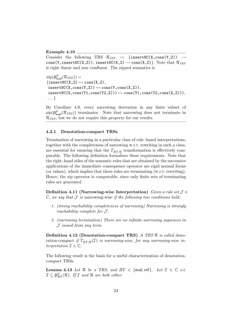
Example 4.10Consider the following TRS RINS := insertNC(X,cons(Y,Z)) →cons(Y,insertNC(X,Z)), insertNC(X,Z)→ cons(X,Z). Note that RINS

is right–linear and non–confluent. The zipped semantics is

zip(BVeval(RINS )) =insertNC(X,Z) 7→ cons(X,Z),insertNC(X,cons(Y,Z)) 7→ cons(Y,cons(X,Z)),insertNC(X,cons(Y1,cons(Y2,Z))) 7→ cons(Y1,cons(Y2,cons(X,Z))),. . .

By Corollary 4.9, every narrowing derivation in any finite subset ofzip(BVeval(RINS )) terminates. Note that narrowing does not terminate inRINS , but we do not require this property for our results.

4.2.1 Denotation-compact TRSs

Termination of narrowing in a particular class of rule–based interpretations,together with the completeness of narrowing w.r.t. rewriting in such a class,are essential for ensuring that the TBT,R transformation is effectively com-putable. The following definition formalizes these requirements. Note thatthe right–hand sides of the semantic rules that are obtained by the successiveapplications of the immediate consequence operator are rigid normal forms(or values), which implies that these rules are terminating (w.r.t. rewriting).Hence, the zip operator is computable, since only finite sets of terminatingrules are generated.

Definition 4.11 (Narrowing-wise Interpretation) Given a rule set J ∈C, we say that J is narrowing-wise if the following two conditions hold:

1. (strong reachability–completeness of narrowing) Narrowing is stronglyreachability–complete for J .

2. (narrowing termination) There are no infinite narrowing sequences inJ issued from any term.

Definition 4.12 (Denotation-compact TRS) A TRS R is called deno-tation-compact if TBT,R(I ) is narrowing-wise, for any narrowing-wise in-terpretation I ∈ C.

The following result is the basis for a useful characterization of denotation-compact TRSs.

Lemma 4.13 Let R be a TRS, and BT ∈ eval, rnf. Let I ∈ C s.t.I ⊆ BVBT (R). If I and R are both either

24

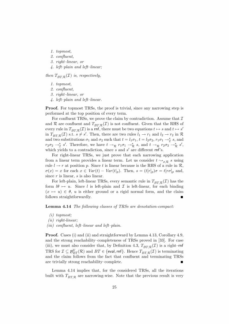
1. topmost,2. confluent,3. right–linear, or4. left–plain and left–linear;

then TBT,R(I ) is, respectively,

1. topmost,2. confluent,3. right–linear, or4. left–plain and left–linear.

Proof. For topmost TRSs, the proof is trivial, since any narrowing step isperformed at the top position of every term.

For confluent TRSs, we prove the claim by contradiction. Assume that Iand R are confluent and TBT,R(I ) is not confluent. Given that the RHS ofevery rule in TBT,R(I ) is a rnf, there must be two equations t 7→ s and t 7→ s′

in TBT,R(I ) s.t. s 6= s′. Then, there are two rules l1 → r1 and l2 → r2 in Rand two substitutions σ1 and σ2 such that t = l1σ1, t = l2σ2, r1σ1 →∗

I s, andr2σ2 →∗

I s′. Therefore, we have t →R r1σ1 →∗R s, and t →R r2σ2 →∗

R s′,which yields to a contradiction, since s and s′ are different rnf’s.

For right-linear TRSs, we just prove that each narrowing applicationfrom a linear term provides a linear term. Let us consider t ;σ,R s usingrule l → r at position p. Since t is linear because is the RHS of a rule in R,σ(x) = x for each x ∈ Var(t) − Var(t|p). Then, s = (t[r]p)σ = t[rσ]p and,since r is linear, s is also linear.

For left-plain, left-linear TRSs, every semantic rule in TBT,R(I ) has theform lθ 7→ u. Since l is left-plain and I is left-linear, for each binding(x 7→ u) ∈ θ, u is either ground or a rigid normal form, and the claimfollows straightforwardly.

Lemma 4.14 The following classes of TRSs are denotation-compact:

(i) topmost;(ii) right-linear;(iii) confluent, left–linear and left–plain.

Proof. Cases (i) and (ii) and straightforward by Lemma 4.13, Corollary 4.9,and the strong reachability–completeness of TRSs proved in [33]. For case(iii), we must also consider that, by Definition 4.3, TBT,R(I ) is a right–rnf

TRS for I ⊆ BVBT (R) and BT ∈ eval, rnf. Hence TBT,R(I ) is terminatingand the claim follows from the fact that confluent and terminating TRSsare trivially strong reachability–complete.

Lemma 4.14 implies that, for the considered TRSs, all the iterationsbuilt with TBT,R are narrowing-wise. Note that the previous result is very

25

handy, since it applies to many TRSs that are commonly used in rewritinglogic and functional programming:

• topmost TRSs and right–linear TRSs, which fulfill the soundness con-ditions for narrowing-based reachability analysis [33], and

• (almost) orthogonal TRSs (a subclass of confluent, left–linear and left–plain TRSs), which fulfill the design conditions of many functionalprogramming languages such as Haskell.

Example 4.15The TRSs RID , RSUM , and RINS of Examples 1.3, 2.1 and 4.10 are right-linear. Thus, by Lemma 4.14, are denotation–compact.

4.2.2 Properties of the Immediate Consequence Operator

In the following, we characterize the properties of the immediate conse-quence operator in narrowing-wise (rule-based) interpretations and denota-tion–compact TRSs.

We prove continuity of the immediate consequence operator in Theo-rem 4.18 below. First, let us demonstrate two auxiliary results. We writet ;! s to denote a narrowing computation from t to a rnf s.

Lemma 4.16 Let I1, I2 ∈ C be narrowing-wise interpretations such thatI1 v I2. Let r, u ∈ T (Σ,V). If r ;!

ρ,I1u, then there are substitutions

η, ρ′, θ and a term u′ ∈ T (Σ,V) such that r ;∗η,I2

u′, ρ|r →∗I2

ρ′, ρ′ = ηθ|r,and u = u′θ.

Proof. r ;!ρ,I1

u implies rρ →!I1

u and, since I1 v I2, rρ →!I2

u. Since I2 isa narrowing-wise interpretation, i.e., by strong–completeness of narrowing,there are substitutions η, ρ′, θ and a term u′ ∈ T (Σ,V) such that r ;∗

η,I2u′,

ρ|r →∗I2

ρ′, ρ′ = ηθ|r, and u = u′θ.

Lemma 4.17 Let I1, I2 ∈ C be narrowing-wise interpretations. If I1 v I2,then TBT,R(I1) v TBT,R(I2).

Proof. Consider t 7→ s ∈ TBT,R(I1). By Lemma 4.16, there are t′ 7→s′ ∈ TBT,R(I2) and a substitution ρ such that t = t′ρ and s = s′ρ. Thus,TBT,R(I2) ` t 7→ s and the conclusion follows.

Theorem 4.18 Let R be a denotation-compact TRS and BT ∈ eval, rnf.The TBT,R operator is continuous w.r.t. v.

Proof. To prove that TBT,R is continuous we can prove that it is monotoneand finitary. It is finitary because of termination of narrowing in narrowing-wise interpretations. Monotonicity follows by Lemma 4.17.

26

Finally, from the soundness of narrowing, the soundness of the TBT,Roperator follows straightforwardly.

Theorem 4.19 (Soundness) Let R be a TRS and BT ∈ eval, rnf. LetI ∈ C s.t. I ⊆ BVBT (R). For each t 7→ s ∈ TBT,R(I ), t →∗

R s.

For interesting classes of TRSs, the fixpoint of the TBT,R transformationcharacterizes the meaning in R of all input calls, which allows us to definea complete compressed fixpoint semantics in the next section.

4.2.3 Fixpoint Compressed Semantics

We are ready to formalize our notion of compressed semantics for TRSs inthe fixpoint style. As usual, we consider the chain of iterations of TBT,Rstarting from the bottom, by defining T 0

BT,R := ∅; T k+1BT,R := TBT,R(T k

BT,R),for k ≥ 0; and Tω

BT,R := tk≥0TkBT,R.

Definition 4.20 (Fixpoint Compressed Semantics) The least fixpointcompressed semantics of a program R is defined as FBT (R) := Tω

BT,R.

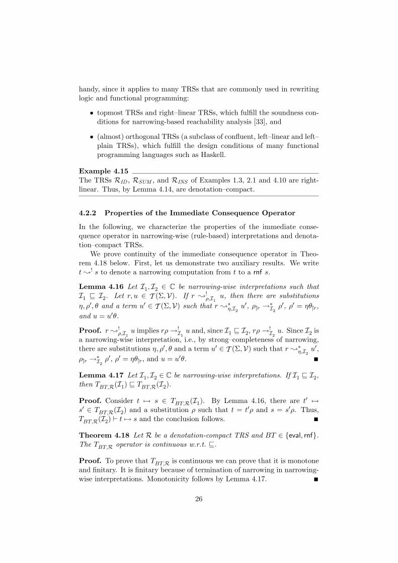
Example 4.21Consider again the TRS RID of Example 1.3. The transformation Trnf,RID

computes the following interpretations: T 1rnf,RID

= T 2rnf,RID

= id(X) 7→ X,which is, thus, the least fixpoint.

We are able to characterize some broad classes of TRSs where the sound-ness and completeness of our compact fixpoint semantics can be proved. Thefollowing definition extends the notion of definedness of a TRS to (possibly)non–confluent TRSs.

Definition 4.22 (BT -defined TRS) We say that t ∈ T (Σ,V) is BT -defined in the TRS R if there exists at least one t′ ∈ BT such that t →!

R t′

and, for all t′′such that t →!R t′′, t′′ ∈ BT .

We say that R is BT -defined (resp. BT -ground-defined) if, for all t ∈T (Σ,V) (resp. t ∈ T (Σ)) t is BT -defined in R.

It is immediate to see that BT -definedness is much more demandingthan BT -ground-definedness. BT -(ground-)definedness has been studied inthe literature for different semantics:

• For the ground value semantics Beval(R), eval-ground-definedness im-plies that nf∩T (Σ) = eval∩T (Σ). Therefore, eval-ground-definednessis equivalent to the condition that R is weakly normalizing and com-pletely defined (CD); see [5]. A TRS R is weakly normalizing if everyterm has a normal form in R, though infinite sequences from t may

27

exist. A TRS R is completely defined if each defined symbol of thesignature is completely defined. In other words, it does not occur inany ground term in normal form, i.e., function symbols are reducibleon all ground terms.

• For the non-ground values semantics BVeval(R), eval-definedness is muchmore demanding, since it requires functions to be reducible on allterms, not only ground terms.

• For the normalization semantics Bnf(R) and BVnf(R), both nf-ground-definedness and nf-definedness are simply equivalent to the notion ofweakly normalizing TRS, which is defined for terms with variables. Itis the same for the semantics of ground rigid normal forms Brnf(R),since Brnf(R) = Bnf(R). However it is more demanding for BVrnf(R)than weakly normalizing, since it requires every term (not only groundterms) to reach a rigid normal form by rewriting.

Example 4.23For BT ∈ eval, rnf, nf, the TRSs RID , RSUM , and RINS of Examples1.3, 2.1 and 4.10 are BT -ground-defined. Only the TRS RID is BT -defined.

Let us also define the class of BT -based TRSs, which generalizes theclass of left-linear constructor systems as follows.

Definition 4.24 (BT -based TRS) Let R be a TRS and BT ∈ evalR,rnfR. A substitution σ is BT–based if, for each X ∈ V, Xσ ∈ BT . Givena TRS R, we call it BT–based if every substitution computed by narrowingin R is BT–based, i.e., for t, t′ ∈ T (Σ,V) such that t ;θ,R t′, θ|t is BT -based.

Popular classes of rnf–based TRSs are:

(i) left–linear constructor systems,(ii) almost orthogonal TRSs, and(iii) topmost TRSs.

Actually, (i) and (ii) are typical functional programs and the class of left–linear constructor systems is exactly the eval-based TRSs, a subclass of rnf-based TRSs. On the other hand, weakly normalizing left–linear constructorsystems are rnf-based as well as rnf-ground-defined. It is worth noting thatrnf–based TRSs are left–plain but not vice versa, as shown in the followingexample.

Example 4.25For BT ∈ eval, rnf, the TRSs RID , RSUM , and RINS of Examples 1.3, 2.1and 4.10 are BT -based, since they are left–linear constructor systems. How-ever, the TRS of Example 4.5 is not BT -based (nor left–plain). Furthermore,

28

the TRS of Example 4.7 is left–plain but not BT -based, since given the term(0 + 0) + Y, we have the narrowing step (0 + 0) + Y ;σ 0 using the ruleX + X→ 0, where the substitution σ = Y 7→ 0 + 0 is not BT -based.

Now we can prove the correctness of the fixpoint semantics w.r.t. theordinary, big–step collecting semantics. The proof of Theorem 4.26 is inAppendix A.

Theorem 4.26 (Ground Soundness and Completeness) Let BT ∈rnf, eval. Let R be either a

• BT -ground-defined, terminating, denotation-compact TRS that is ei-ther confluent or BT -based; or

• topmost TRS.

Then, BBT (R) = unzip(FBT (R)) ∩ (T (Σ)× T (Σ)).

Corollary 4.27 (Correctness w.r.t. Behavior) Let BT ∈ rnf, eval.Let R1,R2 be either

• BT -ground-defined, terminating, denotation-compact TRSs that areeither confluent or BT -based; or

• topmost TRSs.

Then, FBT (R1) = FBT (R2) implies BBT (R1) = BBT (R2).

Note that the conditions that R is BT -based (or confluent), BT -ground-defined, and terminating in the previous result are all necessary. Recall thatdenotation–compactness is required to ensure that narrowing terminates inthe denotation.

Example 4.28Let us consider the following denotation-compact, terminating, eval-basedTRS R := g → f(h(a)), h(a) → s(h(b)), f(s(X)) → a. R is noteval-ground-defined, since e.g. h(a) cannot be rewritten to a value. Now wehave T 1

eval,R = T 2eval,R = f(s(X)) 7→ a. Then, g 7→ a cannot be obtained

from Feval(R).

Example 4.29Let us consider the following denotation-compact, terminating, rnf-ground-defined TRS R := g→ f(h), h→ s(i), i→ a, f(s(a))→ a, f(s(i))→b. R is not rnf-based nor confluent due to the left-hand side f(s(i)).Now we have T 1

rnf,R = i 7→ a, f(s(a)) 7→ a, f(s(i)) 7→ b, T 2rnf,R =

T 1rnf,R ∪ h 7→ s(a), T 3

rnf,R = T 2rnf,R ∪ g 7→ a, and T 4

rnf,R = T 3rnf,R. Then,

g 7→ b cannot be obtained from Frnf(R), whereas g rewrites to b in R.

29

Example 4.30Let us consider the following denotation-compact, eval-ground-defined, eval-based TRS R := g → f(h), h → s(g), f(s(X)) → a. R is not termi-nating, since g → f(h) → f(s(g)) → · · · . Since h and g depend on eachother, we have Feval(R) = f(s(X)) 7→ a, and thus the computations g 7→a and h 7→ s(a) cannot be obtained from Feval(R).

The criteria given in Theorem 4.26 and Corollary 4.27 are reasonable8

for many programming languages such as Maude, Haskell, Scheme, etc.For instance, programs in Haskell are defined as left-linear constructor sys-tems that can be understood as confluent and terminating systems (i.e., theHaskell evaluation strategy always provides, for each input term, one andonly one finite rewriting sequence to a normal form). In Maude, functional(or equational) programs are usually described as (almost) orthogonal, ter-minating TRSs, which is a subclass of confluent, terminating, left–linear,left–plain TRSs; see [10]. Note that much work has been done recentlyto prove termination of functional programs automatically in Maude andHaskell; see [17, 21]. On the other hand, many concurrent systems of in-terest, including the vast majority of distributed algorithms and the opera-tional semantics of many programming languages (Java, JVM bytecode, C,Haskell, Prolog, etc.), admit fairly natural (order-sorted) topmost specifica-tions in Maude; see [32, 33].

Thus we believe that our compression methodology and the results thatwe have proved are quite powerful and practical. In Section 5 we also showmore evidence to support this claim by showing, on various benchmarks,that the fixpoint computation of our semantics produces dramatically fewersemantic rules at each step w.r.t. the big-step semantics.

4.3 Operational (Compressed) Semantics

In this section, we study an operational semantics and compare it with thedenotational semantics provided in Section 3.1.

Definition 4.31 Let R be a TRS and BT ∈ rnf, eval. The OperationalDenotation of R is defined as:

OBT (R) := zip(f(x1, . . . , xn)θ 7→ t | f(x1, . . . , xn) ;∗

θ,R t, t ∈ BT)

where x1, . . . , xn are pairwise distinct variables.

It is easy to prove that this operational semantics captures the observablesof rigid normal forms and values.

8Obviously, these classes of programs can only be considered as the basis of functionalprogramming languages, since many features are not addressed in this paper, such asevaluation strategies, strategy annotations, type systems; or algebraic properties such asassociativity and commutativity, etc.

30

Corollary 4.32 Let R be a strongly reachability–complete TRS and BT ∈rnf, eval. Then, unzip (OBT (R)) = BVBT (R).

Corollary 4.33 (Correctness and Full Abstraction) Let R be a stronglyreachability–complete TRS and BT ∈ rnf, eval. Then, BVBT (R1) = BVBT (R2)if and only if OBT (R1) = OBT (R2).

The optimality of the operational semantics is also straightforward.

Corollary 4.34 (Optimality) Let R be a strongly reachability–completeTRS and BT ∈ rnf, eval. For each S ⊆ BVBT (R) s.t. unzip(S) = BVBT (R),then zip(S) = OBT (R).

The operational semantics in Definition 4.31 is actually equivalent to thefixpoint version, for BT -defined TRSs. The proof of Theorem 4.35 is inAppendix A.

Theorem 4.35 (Equivalence with Denotational Semantics) LetBT ∈ rnf, eval. Let R be either a

• BT -defined, terminating, denotation-compact TRS that is either con-fluent or BT -based; or

• topmost TRS.

Then, FBT (R) = OBT (R).

Here we would like to justify why we have given a bottom-up formaliza-tion for our compressed semantics instead of a simpler top-down operationalsemantics, such as the one in Definition 4.31:

• First, the computation of OBT (R) requires that narrowing terminatesin R, which is more demanding than narrowing termination in theinterpretations obtained from R.

• Second, the set of narrowing sequences in R is not generally finite,which implies that the zip of this set is not effectively computable.

• Third, but not least important, our motivation for the compressed se-mantics comes from a previous work of ours [1] which aimed to extendto TRSs the technique of Abstract Diagnosis [12], originally developedfor Logic Programs, to check the correctness of a TRS. This techniqueis inherently based on the use of an immediate consequence operatorand [12] demonstrated that the resulting methodology is superior thantop-down approaches.

Example 4.36Consider again the TRS RID of Example 1.3, which satisfies the conditionsof Theorem 4.35. We have that Feval(RID) = Oeval(RID) = id(X) 7→ X.

31

However, note that the term id(X) has an infinite number of narrowingderivations, which are only successively collapsed by the zip operation. Thusthe computation of the semantics Oeval(RID) cannot be effectively imple-mented. On the contrary, the computation of Feval(RID) is finite, as shownin Example 4.21.

4.4 Relations with the semantics of [1]

Finally, let us characterize the relationship of our TBT,R transformation withthe more traditional immediate consequence operator given in [1]. Given aset of final/blocking terms BT , in [1] we defined the following naıve imme-diate consequence operator.

Definition 4.37 ([1]) Let R be a TRS, I ∈ S, and BT a set of final/blockingstate pairs. Then,

T unzipBT,R(I ) := BT 2 ∪ s 7→ t ∈ W | r 7→ t ∈ I , s →R r

where BT 2 := t 7→ t | t ∈ BT.

This definition is sensible from a model-theoretic point of view, but itclearly lacks conciseness properties that are critical for analysis and debug-ging. Thus, one could think of using zipped sets as follows:

Definition 4.38 Let R be a TRS, I ∈ C, and BT a set of final/blockingstate pairs. Then,

T zipBT,R(I ) := zip(BT 2 ∪ s 7→ t ∈ W | r 7→ t ∈ unzip(I ), s →R r)

Recall that, in Observation 3.12, we noted that (zip,unzip) is an isomor-phism between compactable unzipped sets and C. Then, it is clear thatthe immediate consequence operator of Definition 4.38 is the operator thatcorresponds to the one of Definition 4.37 by this isomorphism, as formallystated in the following lemma.

Lemma 4.39 Let R be a TRS and BT ∈ rnf, eval. Then, T zipBT,R =

zip T unzipBT,R unzip.

Now, we are able to prove the following result.

Corollary 4.40 Let R be a strongly reachability–complete TRS and BT ∈rnf, eval. Then, FBT (R) = OBT (R) =

(T zip

BT,R)ω.

Actually, the operator T zipBT,R of [1] has a much closer relationship to

operational semantics than to denotational semantics. Indeed, at each ap-plication, it simulates one transition of the rewriting system. In other terms,

32

when applied n times to the bottom element, it will produce (equations cor-responding to) derivations of length exactly n. From a denotational point ofview, this is undesirable, since we would like to take advantage of the factthat, in the interpretation, we already have the information regarding severalderivations (of different length) of various terms all at once. That is why wehave preferred a “true denotational” definition such as Definition 4.3, where,at each iteration, we can produce all rewritings that are possible using “onestep” from the program and all reductions that we already know from thecurrent interpretation.

5 Experimental Results

A proof-of-concept implementation of the compression technique proposed inthis paper has been developed, and used to conduct a number of experimentsthat demonstrate the practicality of our approach. The prototype is writtenin Haskell using the GHC compiler version 6.8.2, and is publicly available9.The tool accepts TRSs that can be written either in TPDB format10, TTTform11, or a subset of the syntax of Maude functional modules.

Since there are many factors that may impact performance and effective-ness when comparing two different implementations, in order to guaranteea fair comparison w.r.t. [1], we have developed a unique fixpoint infrastruc-ture that is parametric on the immediate consequence operator, and wehave evaluated both operators (the compact one proposed in Section 4, andthe one in [1]) within this single framework. In particular, both implemen-tations share the same underlying machinery (unification, narrowing, etc).Furthermore, in order to obtain finite approximations of (possibly) infinitesemantics, we use the depth-k abstraction described in [1], which essentiallycuts the terms in both sides of each semantic rule down to a maximum depthbound, which is fixed by the k parameter; e.g. for depth bound k = 3, theterm plus(0, s(s(s(0)))) is cut down to plus(0, s(s(X))).

In order to assess the practicality of our approach, we have benchmarkedboth the size of the (abstract) fixpoint semantics for a given depth boundand the corresponding computation times. We consider a set of benchmarkprograms that satisfy the conditions for the correctness and completenessof our approach. The benchmarks used for the comparison are: risers andtails, which are two almost–orthogonal and terminating Haskell programsthat are commonly used for analyzing the safety of pattern matching inHaskell [35]; doubleisone, an almost–orthogonal and terminating TRS fordoubling and unity checking borrowed from [24]; bertconc, a right–linear,canonical TRS for concatenating lists borrowed from [7]; vending, a topmost

9At http://safe-tools.dsic.upv.es/zipit10See http://www.lri.fr/∼marche/tpdb/format.html11See http://colo6-c703.uibk.ac.at/ttt/trs.html

33

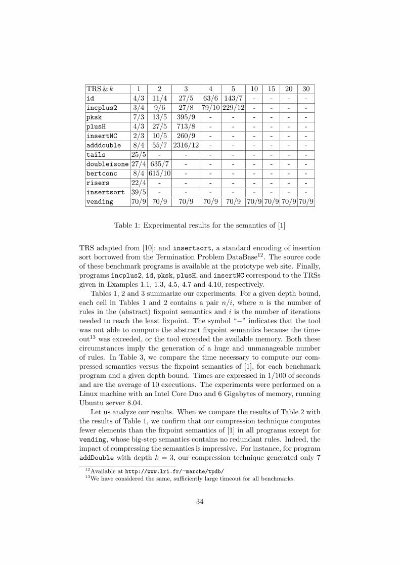
TRS & k 1 2 3 4 5 10 15 20 30id 4/3 11/4 27/5 63/6 143/7 - - - -incplus2 3/4 9/6 27/8 79/10 229/12 - - - -pksk 7/3 13/5 395/9 - - - - - -plusH 4/3 27/5 713/8 - - - - - -insertNC 2/3 10/5 260/9 - - - - - -adddouble 8/4 55/7 2316/12 - - - - - -tails 25/5 - - - - - - - -doubleisone 27/4 635/7 - - - - - - -bertconc 8/4 615/10 - - - - - - -risers 22/4 - - - - - - - -insertsort 39/5 - - - - - - - -vending 70/9 70/9 70/9 70/9 70/9 70/9 70/9 70/9 70/9

Table 1: Experimental results for the semantics of [1]

TRS adapted from [10]; and insertsort, a standard encoding of insertionsort borrowed from the Termination Problem DataBase12. The source codeof these benchmark programs is available at the prototype web site. Finally,programs incplus2, id, pksk, plusH, and insertNC correspond to the TRSsgiven in Examples 1.1, 1.3, 4.5, 4.7 and 4.10, respectively.

Tables 1, 2 and 3 summarize our experiments. For a given depth bound,each cell in Tables 1 and 2 contains a pair n/i, where n is the number ofrules in the (abstract) fixpoint semantics and i is the number of iterationsneeded to reach the least fixpoint. The symbol “−” indicates that the toolwas not able to compute the abstract fixpoint semantics because the time-out13 was exceeded, or the tool exceeded the available memory. Both thesecircumstances imply the generation of a huge and unmanageable numberof rules. In Table 3, we compare the time necessary to compute our com-pressed semantics versus the fixpoint semantics of [1], for each benchmarkprogram and a given depth bound. Times are expressed in 1/100 of secondsand are the average of 10 executions. The experiments were performed on aLinux machine with an Intel Core Duo and 6 Gigabytes of memory, runningUbuntu server 8.04.

Let us analyze our results. When we compare the results of Table 2 withthe results of Table 1, we confirm that our compression technique computesfewer elements than the fixpoint semantics of [1] in all programs except forvending, whose big-step semantics contains no redundant rules. Indeed, theimpact of compressing the semantics is impressive. For instance, for programaddDouble with depth k = 3, our compression technique generated only 7

12Available at http://www.lri.fr/∼marche/tpdb/13We have considered the same, sufficiently large timeout for all benchmarks.

34

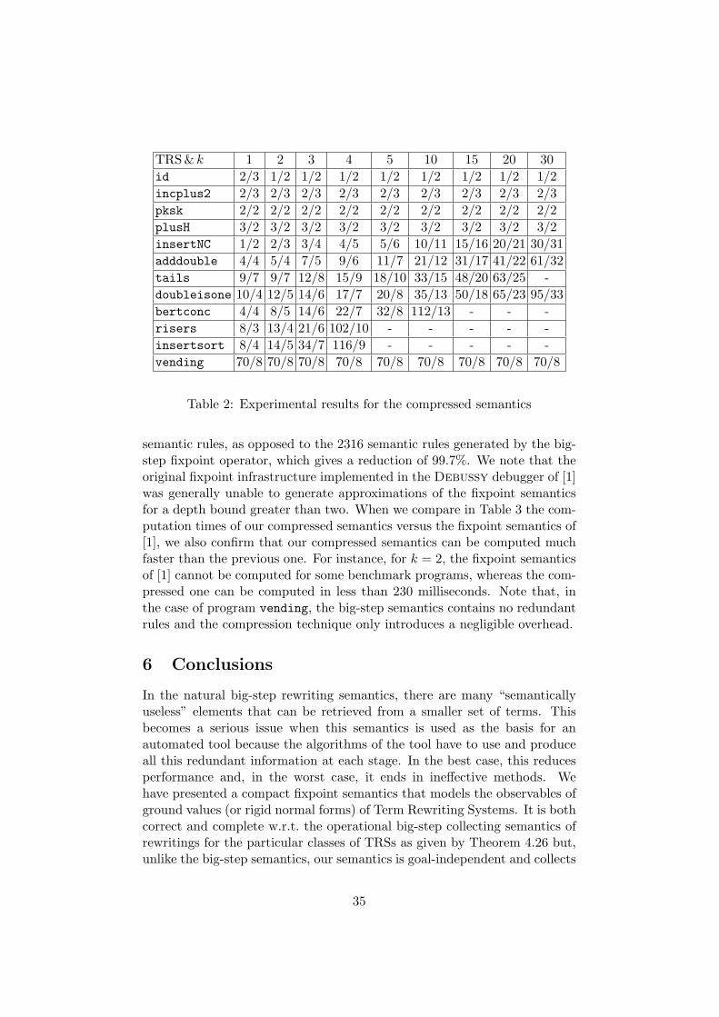
TRS & k 1 2 3 4 5 10 15 20 30id 2/3 1/2 1/2 1/2 1/2 1/2 1/2 1/2 1/2incplus2 2/3 2/3 2/3 2/3 2/3 2/3 2/3 2/3 2/3pksk 2/2 2/2 2/2 2/2 2/2 2/2 2/2 2/2 2/2plusH 3/2 3/2 3/2 3/2 3/2 3/2 3/2 3/2 3/2insertNC 1/2 2/3 3/4 4/5 5/6 10/11 15/16 20/21 30/31adddouble 4/4 5/4 7/5 9/6 11/7 21/12 31/17 41/22 61/32tails 9/7 9/7 12/8 15/9 18/10 33/15 48/20 63/25 -doubleisone 10/4 12/5 14/6 17/7 20/8 35/13 50/18 65/23 95/33bertconc 4/4 8/5 14/6 22/7 32/8 112/13 - - -risers 8/3 13/4 21/6 102/10 - - - - -insertsort 8/4 14/5 34/7 116/9 - - - - -vending 70/8 70/8 70/8 70/8 70/8 70/8 70/8 70/8 70/8

Table 2: Experimental results for the compressed semantics

semantic rules, as opposed to the 2316 semantic rules generated by the big-step fixpoint operator, which gives a reduction of 99.7%. We note that theoriginal fixpoint infrastructure implemented in the Debussy debugger of [1]was generally unable to generate approximations of the fixpoint semanticsfor a depth bound greater than two. When we compare in Table 3 the com-putation times of our compressed semantics versus the fixpoint semantics of[1], we also confirm that our compressed semantics can be computed muchfaster than the previous one. For instance, for k = 2, the fixpoint semanticsof [1] cannot be computed for some benchmark programs, whereas the com-pressed one can be computed in less than 230 milliseconds. Note that, inthe case of program vending, the big-step semantics contains no redundantrules and the compression technique only introduces a negligible overhead.

6 Conclusions

In the natural big-step rewriting semantics, there are many “semanticallyuseless” elements that can be retrieved from a smaller set of terms. Thisbecomes a serious issue when this semantics is used as the basis for anautomated tool because the algorithms of the tool have to use and produceall this redundant information at each stage. In the best case, this reducesperformance and, in the worst case, it ends in ineffective methods. Wehave presented a compact fixpoint semantics that models the observables ofground values (or rigid normal forms) of Term Rewriting Systems. It is bothcorrect and complete w.r.t. the operational big-step collecting semantics ofrewritings for the particular classes of TRSs as given by Theorem 4.26 but,unlike the big-step semantics, our semantics is goal-independent and collects

35

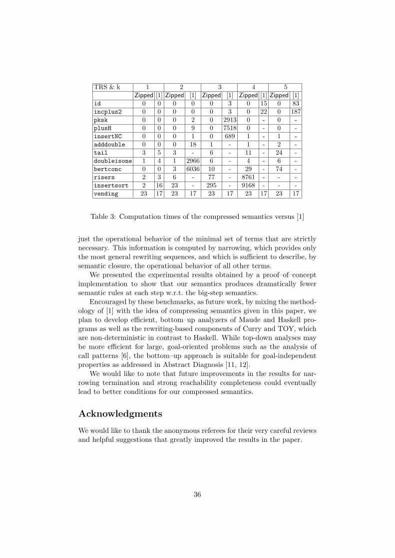
TRS & k 1 2 3 4 5Zipped [1] Zipped [1] Zipped [1] Zipped [1] Zipped [1]

id 0 0 0 0 0 3 0 15 0 83incplus2 0 0 0 0 0 3 0 22 0 187pksk 0 0 0 2 0 2913 0 - 0 -plusH 0 0 0 9 0 7518 0 - 0 -insertNC 0 0 0 1 0 689 1 - 1 -adddouble 0 0 0 18 1 - 1 - 2 -tail 3 5 3 - 6 - 11 - 24 -doubleisone 1 4 1 2966 6 - 4 - 6 -bertconc 0 0 3 6036 10 - 29 - 74 -risers 2 3 6 - 77 - 8761 - - -insertsort 2 16 23 - 295 - 9168 - - -vending 23 17 23 17 23 17 23 17 23 17

Table 3: Computation times of the compressed semantics versus [1]

just the operational behavior of the minimal set of terms that are strictlynecessary. This information is computed by narrowing, which provides onlythe most general rewriting sequences, and which is sufficient to describe, bysemantic closure, the operational behavior of all other terms.

We presented the experimental results obtained by a proof–of–conceptimplementation to show that our semantics produces dramatically fewersemantic rules at each step w.r.t. the big-step semantics.

Encouraged by these benchmarks, as future work, by mixing the method-ology of [1] with the idea of compressing semantics given in this paper, weplan to develop efficient, bottom–up analyzers of Maude and Haskell pro-grams as well as the rewriting-based components of Curry and TOY, whichare non-deterministic in contrast to Haskell. While top-down analyses maybe more efficient for large, goal-oriented problems such as the analysis ofcall patterns [6], the bottom–up approach is suitable for goal-independentproperties as addressed in Abstract Diagnosis [11, 12].

We would like to note that future improvements in the results for nar-rowing termination and strong reachability completeness could eventuallylead to better conditions for our compressed semantics.

Acknowledgments

We would like to thank the anonymous referees for their very careful reviewsand helpful suggestions that greatly improved the results in the paper.

36

References

[1] M. Alpuente, M. Comini, S. Escobar, M. Falaschi, and S. Lucas. Ab-stract Diagnosis of Functional Programs. In M. Leuschel, editor, LogicBased Program Synthesis and Transformation – 12th InternationalWorkshop, LOPSTR 2002, Revised Selected Papers, volume 2664 ofLecture Notes in Computer Science, pages 1–16, Berlin, 2003. Springer-Verlag.

[2] M. Alpuente, F. J. Correa, and M. Falaschi. A Declarative DebuggingScheme for Functional Logic Programs. In M. Hanus, editor, Proceed-ings of 10th International Workshop on Functional and (Constraint)Logic Programming (WFLP 2001), volume 64 of Electronic Notes inTheoretical Computer Science, North Holland, 2002. Elsevier SciencePublishers.

[3] M. Alpuente, S. Escobar, and J. Iborra. Termination of narrowingrevisited. Theoretical Computer Science, 410(46):4608–4625, 2009.

[4] M. Alpuente, M. Falaschi, M. J. Ramis, and G. Vidal. A CompositionalSemantics for Conditional Term Rewriting Systems. In H. E. Bal, ed-itor, Proc. of 6th IEEE Int’l Conf. on Computer Languages, ICCL’94,pages 171–182, Los Alamitos, CA, USA, 1994. IEEE Computer SocietyPress.

[5] F. Baader and T. Nipkow. Term Rewriting and All That. CambridgeUniversity Press, Cambridge, UK, 1998.

[6] R. Barbuti, R. Giacobazzi, and G. Levi. A General Frameworkfor Semantics-based Bottom-up Abstract Interpretation of Logic Pro-grams. ACM Transactions on Programming Languages and Systems,15(1):133–181, 1993.

[7] D. Bert, R. Echahed, and B. M. Østvold. Abstract Rewriting. In Pro-ceedings of Third Int’l Workshop on Static Analysis (WSA’93), volume724 of Lecture Notes in Computer Science, pages 178–192, Berlin, 1993.Springer-Verlag.

[8] A. Bossi, M. Gabbrielli, G. Levi, and M. Martelli. The s-semanticsapproach: Theory and applications. Journal of Logic Programming,19–20:149–197, 1994.

[9] J. Christian. Some Termination Criteria for Narrowing and E-Narrowing. In Automated Deduction—CADE-11, volume 607 of LectureNotes in Computer Science, pages 582–588. Springer-Verlag, Berlin,1992.

37

[10] M. Clavel, F. Duran, S. Eker, P. Lincoln, N. Martı-Oliet, J. Meseguer,and C. Talcott. All About Maude - A High-Performance Logical Frame-work: How to Specify, Program, and Verify Systems in Rewriting Logic,volume 4350 of Lecture Notes in Computer Science. Springer-Verlag,Berlin, 2007.

[11] M. Comini, G. Levi, M. C. Meo, and G. Vitiello. Proving propertiesof Logic Programs by Abstract Diagnosis. In M. Dams, editor, Pro-ceedings of Analysis and Verification of Multiple-Agent Languages, 5thLOMAPS Workshop (LOMAPS’96), volume 1192 of Lecture Notes inComputer Science, pages 22–50, Berlin, 1996. Springer-Verlag.

[12] M. Comini, G. Levi, M. C. Meo, and G. Vitiello. Abstract Diagnosis.Journal of Logic Programming, 39(1-3):43–93, 1999.

[13] H. Comon-Lundh. Intruder Theories (Ongoing Work). In ProceedingsFoSSaCS 2004, volume 2987 of Lecture Notes in Computer Science,pages 1–4. Springer-Verlag, 2004.

[14] V. Cortier, S. Delaune, and P. Lafourcade. A Survey of Algebraic Prop-erties used in Cryptographic Protocols. Journal of Computer Security,14(1):1–43, 2006.

[15] P. Cousot and R. Cousot. Abstract Interpretation: A Unified LatticeModel for Static Analysis of Programs by Construction or Approxima-tion of Fixpoints. In Proceedings of the 4th ACM SIGACT-SIGPLANsymposium on Principles of programming languages, Los Angeles, Cal-ifornia, January 17–19, pages 238–252, New York, NY, USA, 1977.ACM Press.

[16] N. Dershowitz and J.-P. Jouannaud. Rewrite Systems. In J. vanLeeuwen, editor, Handbook of Theoretical Computer Science, volumeB: Formal Methods and Semantics, chapter 6, pages 244–320. Elsevier,1990.

[17] F. Duran, S. Lucas, and J. Meseguer. MTT: The Maude Termina-tion Tool (System Description). In A. Armando, P. Baumgartner, andG. Dowek, editors, Automated Reasoning, 4th International Joint Con-ference, IJCAR 2008, Proceedings, volume 5195 of Lecture Notes inComputer Science, pages 313–319. Springer-Verlag, 2008.

[18] M. Falaschi, G. Levi, M. Martelli, and C. Palamidessi. A new Declar-ative Semantics for Logic Languages. In R. A. Kowalski and K. A.Bowen, editors, Proceedings of Fifth Int’l Conf. on Logic Programming,pages 993–1005, Cambridge, Mass., 1988. The MIT Press.

38

[19] M. Falaschi, G. Levi, M. Martelli, and C. Palamidessi. DeclarativeModeling of the Operational Behavior of Logic Languages. TheoreticalComputer Science, 69(3):289–318, 1989.

[20] M. Fay. First-Order Unification in an Equational Theory. In FourthInt’l Conf. on Automated Deduction, pages 161–167, 1979.

[21] J. Giesl, S. Swiderski, P. Schneider-Kamp, and R. Thiemann. Auto-mated Termination Analysis for Haskell: From Term Rewriting to Pro-gramming Languages. In Frank Pfenning, editor, Term Rewriting andApplications, 17th International Conference, RTA 2006, Proceedings,volume 4098 of Lecture Notes in Computer Science, pages 297–312.Springer-Verlag, 2006.

[22] M. Hanus. The Integration of Functions into Logic Programming: FromTheory to Practice. Journal of Logic Programming, 19&20:583–628,1994.

[23] M. Hanus. Multi-paradigm Declarative Languages. In V. Dahl andI. Niemela, editors, Logic Programming, 23rd International Conference,ICLP 2007, Proceedings, volume 4670 of Lecture Notes in ComputerScience, pages 45–75. Springer-Verlag, 2007.

[24] M. Hanus. Call Pattern Analysis for Functional Logic Programs. InProceedings 10th Int’l ACM SIGPLAN Conf. on Principle and Prac-tice of Declarative Programming (PPDP’08), pages 67–78. ACM Press,2008.

[25] Haskell Debugging Technologies. At http://www.haskell.org/debugging/, October 2008.

[26] J.-M. Hullot. Canonical Forms and Unification. In Proceedings ofthe 5th International Conference on Automated Deduction, volume 87of Lecture Notes in Computer Science, pages 318–334, Berlin, 1980.Springer-Verlag.

[27] J.-M. Hullot. Canonical Forms and Unification. In Proceedings of the5th International Conference on Automated Deduction [26], pages 318–334.

[28] J. W. Klop. Term Rewriting Systems. In S. Abramsky, D. M. Gabbay,and T. S. E. Maibaum, editors, Handbook of Logic in Computer Science,volume I, pages 1–112. Oxford University Press, 1992.

[29] D. E. Knuth and P. B. Bendix. Simple Word Problems in UniversalAlgebras. In Computational Problems in Abstract Algebra, pages 263–297, 1970.

39

[30] F.J. Lopez-Fraguas and J. Sanchez-Hernandez. TOY: A MultiparadigmDeclarative System. In Proc. of 10th International Conference onRewriting Techniques and Applications, RTA 1999, volume 1631 of Lec-ture Notes in Computer Science, pages 244–247. Springer-Verlag, 1999.

[31] S. Marlow, J. Iborra, B. Pope, and A. Gill. A Lightweight InteractiveDebugger for Haskell. In G. Keller, editor, Proceedings of the ACMSIGPLAN Workshop on Haskell (Haskell 2007), pages 13–24. ACMPress, 2007.

[32] J. Meseguer and G. Rosu. The Rewriting Logic Semantics Project.Theoretical Computer Science, 373(3):213–237, 2007.

[33] J. Meseguer and P. Thati. Symbolic reachability analysis using nar-rowing and its application to verification of cryptographic protocols.Higher-Order and Symbolic Computation, 20(1-2):123–160, 2007.

[34] A. Middeldorp and E. Hamoen. Completeness Results for Basic Nar-rowing. Journal of Applicable Algebra in Engineering, Communicationand Computing, 5:313–353, 1994.

[35] N. Mitchell and C. Runciman. A Static Checker for Safe Pattern Match-ing in Haskell. In M. Van Eekelen, editor, Trends in Functional Pro-gramming, volume 6, pages 15–30. Intellect, 2007.

[36] H. R. Nielson and F. Nielson. Infinitary Control Flow Analysis: aCollecting Semantics for Closure Analysis. In Symposium on Principlesof Programming Languages, pages 332–345, 1997.

[37] S. Peyton Jones. Haskell 98 Language and Libraries: the Revised Re-port. Cambridge University Press, 2003.

[38] R. Plasmeijer and M. van Eekelen. Functional Programming and Par-allel Graph Rewriting. Addison-Wesley, Reading, MA, 1993.

[39] TeReSe, editor. Term Rewriting Systems. Cambridge University Press,Cambridge, UK, 2003.

[40] P. Wadler. An angry half-dozen. SIGPLAN Notices, 33(2):25–30, 1998.

40

A Proof of main theorems

The following result is the basis for the main theorems below. We usenotation t →n

R s to represent a rewrite sequence from t to s consisting of nsteps.

Lemma A.1 Let BT ∈ rnf, eval. Let R be a BT -defined, terminating,denotation-compact TRS that is either confluent or BT -based. Let t, s ∈T (Σ,V). If t 7→ s ∈ BVBT (R), then FBT (R) ` t 7→ s.

Proof. First, consider the maximal context C[ ] with m holes at disjointpositions p1, . . . , pm such that t = C[u1, . . . , um], s = C[v1, . . . , vm], andv1, . . . , vm ∈ BT . Since C[ ] is maximal, each sequence uj →∗

R vj containsat least one rewriting step at the top position. In the following, we provethat FBT (R) ` uj 7→ vj for each j = 1, . . . ,m, and thus the conclusionfollows.

Let u, v ∈ T (Σ,V) and v ∈ BT such that u →∗R v contains at least one

rewriting step at the top position. Since R is terminating, we consider thelongest rewrite derivation from u to v, i.e., u = t0

p1→R t1 . . .pn→R tn = v.

Let k ∈ 1, . . . , n be such that pk is the first top position in the sequencep1, . . . , pn. The derivation can be split into three parts t0 →n1

R tk−1ε→R

tk →n2R tn. Then, we prove FBT (R) ` t0 7→ tn by induction on n = n1+n2+1.

n1 = 0 & n2 = 0)

Here we have that t0ε→l→r tn where l → r ∈ R and ρ is

the applied substitution, i.e., t0 = lρ and tn = rρ. Note that r ∈ BT ,since rρ ∈ BT . Thus, by definition, l 7→ r has been eventually addedto the fixpoint (though possibly removed after the zip compression);hence, FBT (R) ` l 7→ r, which implies FBT (R) ` t0 7→ tn.

n1 > 0 or n2 > 0)

Here we have t0 →n1R tk−1

ε→l→r tk →n2R tn where

l → r ∈ R and tn ∈ BT . Following the same reasoning as in thegeneral case given at the beginning of this proof, there is a maximalcontext C[ ] with m holes at disjoint positions q1, . . . , qm such thatt0 = C[u1, . . . , um] and tk−1 = C[u′1, . . . , u

′m]. Now, since pk is the

first reduced top position, C[ ] is different from the empty context.

Note that u′1, . . . , u′m do not necessarily belong to BT . Let ρ = x1 7→

w1, . . . , xnρ 7→ wnρ be such that tk−1 = lρ and tk = rρ. Assume ρ isnot BT -based. Since R is BT -defined, there is a BT -based substitu-tion ρ = x1 7→ w1, . . . , xnρ 7→ wnρ such that for each i ∈ 1, . . . , nρ,wi →hi

R wi and, since n is the length of the longest derivation from t0,then hi < n. Then, by the induction hypothesis, FBT (R) ` wi 7→ wi

for each i ∈ 1, . . . , nρ. Let tk−1 = lρ. Thus, FBT (R) ` tk−1 7→ tk−1,since the maximal context C[ ] of tk−1 and tk−1 is the same.

Now, we consider the cases when R is confluent and R is BT -basedseparately.

41

R is confluent)

Then, rρ →∗R tn. By the induction hypothesis,

FBT (R) ` tk−1 7→ tn. Since FBT (R) is narrowing-wise and ρis BT -based, there are substitutions η, θ and a term t′n ∈ T (Σ,V)such that r ;∗

η,FBT (R) t′n, ρ|r = (ηθ)|r, and tn = t′nθ. Thus,by definition, lη 7→ t′n has eventually been added to the fix-point (though possibly removed) and FBT (R) ` lη 7→ t′n. FinallyFBT (R) ` t0 7→ tn, since t0 →∗

FBT (R) tk−1 →FBT (R) rρ →∗FBT (R)

t′nθ = tn.

R is BT -based)

Since FBT (R) is narrowing-wise, there are substi-tutions η, ρ′, θ and a term t′n ∈ T (Σ,V) such that r ;∗

η,FBT (R) t′n,ρ|r →∗

R ρ′, ρ′|r = (ηθ)|r, and tn = t′nθ. Thus, by definition, lη 7→t′n has eventually been added to the fixpoint (though possibly re-moved) and FBT (R) ` lη 7→ t′n. Since we do not require conflu-ence, there may be several possible terms wi,1, . . . , wi,ni,ρ for eachi ∈ 1, . . . , nρ. Note that ρ′, η, θ are BT -based, since tn ∈ BT .Therefore, we arbitrarily choose a wi,j that is compatible withthe substitution ρ′, i.e., we choose wi,j , j ∈ 1, . . . , ni,ρ, for eachi ∈ 1, . . . , nρ such that ρ|r = ρ′|r. Finally, FBT (R) ` t0 7→ tn,since t0 →∗

FBT (R) tk−1 →FBT (R) rρ →∗FBT (R) t′nθ = tn.

Lemma A.2 Let BT ∈ rnf, eval. Let R be a topmost TRS. Let t, s ∈T (Σ,V). If t 7→ s ∈ BVBT (R), then FBT (R) ` t 7→ s.

Proof. Let u, v ∈ T (Σ,V) and v ∈ BT such that u →∗R v. Since R is

topmost, every rewriting step is performed at the top position, i.e., we con-sider u = t0

ε→R t1 . . .ε→R tn = v. Then, we prove FBT (R) ` t0 7→ tn by

induction on n.

n = 0)

Immediate, since t0 = tn ∈ BT .

n > 0)

Here we have t0ε→l→r t1 →n−1

R tn where l → r ∈ R, tn ∈ BT , andt1 = rρ for some substitution ρ. Since FBT (R) is narrowing-wise byLemma 4.14, there are substitutions η, θ and a term t′n ∈ T (Σ,V) suchthat r ;∗

η,FBT (R) t′n, ρ|r = (ηθ)|r, and tn = t′nθ. Thus, by definition,lη 7→ t′n has eventually been added to the fixpoint (though possiblyremoved) and FBT (R) ` lη 7→ t′n. Finally, FBT (R) ` t0 7→ tn, sincet0 = lρ →FBT (R) t1 = rρ →∗

FBT (R) tn = t′nθ.

In the following, we exchange the order of appearance of Theorems 4.26and 4.35 for simplicity.

Theorem 4.35 (Equivalence with Denotational Semantics) Let BT∈ rnf, eval. Let R be either a

42

• BT -defined, terminating, denotation-compact TRS that is either con-fluent or BT -based; or

• topmost TRS.

Then, FBT (R) = OBT (R).

Proof. Consider the case when R is a BT -defined, terminating, denotation-compact TRS that is either confluent or BT -based. First note that, byCorollary 4.32, OBT (R) = zip(BVBT (R)). If t 7→ s ∈ FBT (R), then t 7→s ∈ zip(BVBT (R)) by Theorem 4.19. If t 7→ s ∈ zip(BVBT (R)), then t 7→s ∈ FBT (R) by Lemma A.1.

If R is a topmost TRS, then the proof is similar but using Lemma A.2instead of Lemma A.1.

Theorem 4.26 (Soundness and Completeness) Let BT ∈ rnf, eval.Let R be either a

• BT -ground-defined, terminating, denotation-compact TRS that is ei-ther confluent or BT -based; or

• topmost TRS.

Then, BBT (R) = unzip(FBT (R)) ∩ (T (Σ)× T (Σ)).

Proof. The proof is perfectly analogous to the proof of Theorem 4.35 byreplacing BT -definedness with the less restrictive BT -ground-definednesscondition. This is because ground terms can be rewritten only to groundterms when no extra variables are allowed in right–hand sides of rules.

43

B More properties of zip/unzip

We show here, in more details, what happens in the general case of dealingwith interpretations that are not necessarily compactable. Given I ⊆ W,we say I is meaningless if it contains only semantic rules of the form t 7→ t;and meaningful otherwise. Note that meaningless sets generate, by rewritingconsequences, only meaningless sets and meaningful sets cannot be obtainedby rewriting consequences from meaningless sets.

First, we provide a generic notion of semantic generator.

Definition B.1 (Generator Subset) Given I ⊆ W, we say that G ⊆ Iis a generator subset of I, written G ⊂

→ I, if

1. G ` I (i.e., I ⊆ unzip(G)), and2. ∀r ∈ G, G− r / r (i.e., zip(G) = G).

By allgens(I) we denote the set of all generators, i.e., allgens(I) = G |G ⊂

→ I.

When G ⊂→ I, all elements in I − G are (roughly speaking) “redundant

elements” of I that can be reconstructed from G. Note that, excluded thedegenerate case of meaningless interpretations, generators are non-empty(i.e., G = ∅ cannot be a generator of a meaningful I).

Moreover, note that

• for any G ⊂→ I, unzip(G) = unzip(I)

because G ⊆ I implies unzip(G) ⊆ unzip(I), by Point 2 of Proposi-tion 3.11, and I ⊆ unzip(G) implies unzip(I) ⊆ unzip(G), by Points 2and 1 of Proposition 3.11.

• G ⊂→ I if and only if G ⊆ I, zip(G) = G, unzip(G) = unzip(I)

the “only if” comes from Definition B.1 and the previous point andthe vice versa since unzip(G) = unzip(I) implies G ` I.

• allgens(I) = X ⊆ I | zip(X) = X, unzip(X) = unzip(I)immediate from the previous point.

• a generator G cannot be properly contained into another generator G′

otherwise, for r ∈ G′−G, G ` r and, since G ⊆ G′−r, G′−r ` r,contradicting that G′ is a generator

Generator subsets may not be unique and all possible generators are notnecessarily of the same cardinality, as shown in the following example.

Example B.2Consider again the set I of Example 3.9. According to Definition B.1 thereare several possible generators of I:

44

1. a 7→ b, b 7→ c, c 7→ a,2. b 7→ a, c 7→ b, a 7→ c,3. a 7→ b, b 7→ a, a 7→ c, c 7→ a,4. b 7→ c, c 7→ b, a 7→ c, c 7→ a,5. a 7→ b, b 7→ a, b 7→ c, c 7→ b,

Note that, e.g. a 7→ b, b 7→ c, c 7→ a ` b 7→ a.

Nevertheless, there is no “internal” redundancy in any such a generatorsubset and all the original elements can be reconstructed from it. In thissense, the actual choice of a generator subset can be considered irrelevant.Moreover, in Corollary B.8 below we prove that a unique, minimal generatorsubset exists for any meaningful I ⊆ BVrnf(R) (and thus I ⊆ BVeval(R)).Actually, for these semantics, Definition B.1 boils down to the operator zipas given in Definition 3.7.

Note that, in general, zip(I) is not necessarily a generator of I, as wealready showed in Example 3.9. However, if for any r ∈ I we have I − r /r, then A − r / r for each A ⊆ I. This implies that zip(I) is containedin any generator of I. However, the fact that zip(I) is not a generator ofI does not generally imply zip(I) = ∅. For instance, if we consider the setI ′ := I∪a 7→ d for the set I of Example 3.9, we have that zip(I ′) = a → dand zip(I ′) is not a generator of I ′.

The interesting thing is that, even when zip fails to work, generatorsubsets may exist (as shown by Examples B.2 and 3.9).

Moreover it is possible to define an increasing succession of subsets of Iwhose limit is exactly one generator of I. Unfortunately we are not guaran-teed that the limit always exist.

Proposition B.3 For any meaningful I ⊆ W it is possible to define a suc-cession of subsets of I, such that its limit (if it exists) is one generator subsetof I.

Proof. Let us consider two meaningful sets I1, I2, we say that I1 I2 iffunzip(I1) ⊂ unzip(I2) or unzip(I1) = unzip(I2) and I1 ⊆ I2. Let us notethat is a partial order and that I1 I2 =⇒ I2 ` I1.Thus, let us choose any arbitrary total ordering of I := e1, e2, . . . (this ispossible since W is countably infinite). Let us define inductively G1 := e1and

Gi+1 :=

Gi if Gi ` ei+1

reduce(Gi ∪ ei+1) otherwise

where, for a finite set F = e′1, . . . , e′m, reduce(F ) := Fm where the Fi areiteratively defined as F0 := F and

Fi+1 :=

Fi if Fi − e′i+1 6` e′i+1

Fi − e′i+1 otherwise

45

It is easy to see that for F ′ = reduce(F ), F ′ ⊆ F , F ′ ` F , and for allr ∈ F ′, F ′ − r / r, i.e., reduce(F ) ⊂

→ F . By induction hypothesis, Gi isnon empty, Gi ` Gi−1, Gi ` e1, . . . , ei and ∀r ∈ Gi, Gi − r / r. Now wecan conclude that Gi+1 is non empty, Gi+1 ` Gi, Gi+1 ` e1, . . . , ei+1 and∀r ∈ Gi+1, Gi+1−r / r. Now, in case that I is finite, i.e. I = e1, . . . , enwe can conclude that Gn+1 is a generator for I, since Gn ` e1, . . . , en andsince ∀r ∈ Gn, Gn − r / r. Let us thus consider the case in which I isinfinite. Clearly the sequence G1, G2, . . . will also be infinite. Let us notethat this sequence is a chain, i.e. ∀i ∈ ω.Gi Gi+1. We will now showthat if this chain has a least upper bound, such element is one generator ofI. In fact, let G :=

⊔i Gi. Then, since G is an upper bound, ∀i ∈ ω.Gi

G, and hence G ` Gi ` e1, . . . , ei, and hence G ` I. Furthermore, Gis not redundant, i.e. ∀r ∈ G.G − r / r. In fact, there are only twopossibilities: either (1) there exists j < ω such that unzip(Gj) = unzip(G),and hence clearly Gj = G, and Gj is not redundant by construction or (2)∀i < ω. unzip(Gi) ⊂ unzip(G). Then, let us assume by contradiction thatG is redundant, and that there exists ej ∈ G such that G − ej ` ej.Then, ∀i < ω.unzip(Gi) ⊂ unzip(G) = unzip(G− ej). Hence G − ejwould be an upper bound strictly smaller than the least upper bound G,which is absurd. Finally, let us prove that G ⊆ I. In fact, I is an upperbound for the set G1, G2, . . ., and hence the least upper bound G I,and I ` G. Since we proved that G ` I, then unzip(G) = unzip(I), andhence G I =⇒ G ⊆ I.

Clearly depending on the chosen total ordering on I we can have differentgenerators.

Finally, let us observe that the existence of the least upper bound is notguaranteed for any possible input set I.

The following proposition shows that the construction presented in Propo-sition B.3 is a generalization of the notion of zip, which is retrieved as aparticular case when the conditions of Lemma 3.16 holds.

Proposition B.4 Let BT ∈ evalR, rnfR, and I ⊆ BVBT (R) then zip(I)is the least upper bound of the sequence of sets constructed for the set I inProposition B.3.

Proof. Let us first note that By Lemma 3.16, zip(I) ` I, zip(I) is an upperbound for the sequence G1, G2, . . ., constructed in Proposition B.3. Thenlet us prove that it is the least upper bound. In Proposition B.3 we showedthat the least upper bound, if it exists, is a subset of I, and that for anyupper bound G, G ` I. Thus, let us consider an upper bound G ⊆ I. Nowwe prove that zip(I) ⊆ G, and hence that zip(I) is the least upper bound.By contradiction, assume that there exists r ∈ zip(I) such that r 6∈ G. Bydefinition of zip(I), I−r / r and clearly since G ⊆ I, G = G−r / r ∈ I,which is absurd.

46

Let us now restrict our attention to meaningful sets that have a gen-erator, which we call weakly compactable. Clearly meaningful compactablesets are weakly compactable and (as shown by Examples B.2 and 3.9) theviceversa is not true.

The following proposition shows that the notion of generator of Defini-tion B.1 is a generalization of the notion of zip, because when zip(I) ` Ithen zip(I) is the unique generator of I.

Proposition B.5 For any weakly compactable I ⊆ W,

1. zip(I) ⊆⋂

allgens(I) (=⋂G | G ⊂

→ I).

2. If zip(I) is a generator of I then it is the unique generator of I.

Proof. First of all note that, since I is weakly compactable, I 6= ∅ andallgens(I) 6= ∅.

For Point 1, the case where I is a singleton is straightforward.Otherwise, let us recall that if for any r ∈ I we have that I − r / r,

then for any G ∈ allgens(I) we have that G − r / r, r ∈ zip(I), andzip(I) ⊆ G. Thus zip(I) ⊆

⋂allgens(I).

For Point 2, if zip(I) is a generator, by the fact that generators cannotbe properly contained, then zip(I) has to be the unique generator.

The following results are straightforward consequences of the two previ-ous propositions.

Corollary B.6 If I is compactable, then zip(I) is the unique generator ofI.

Proof. It follows from Proposition B.5 by the fact that zip(I) ` I.

Corollary B.7 If I is zipped, then it is the unique generator of itself.

Finally, we show that zip is the unique generator for BT ∈ evalR, rnfR.

Corollary B.8 For BT ∈ evalR, rnfR and a set I ⊆ BVBT (R), zip(I) isthe unique generator subset of I according to Definition B.1.

Proof. By Corollary B.6 it suffices to prove that zip(I) ` I. But this followsfrom Lemma 3.16.

Note that Corollary B.8 only holds for BT ∈ evalR, rnfR, as it is witnessedby the following counter-example.

Example B.9Consider again the interpretation I of Example B.2, which consider seman-tics BVred(R). According to Definition B.1 there are two minimal generatorsof I: a 7→ b, b 7→ c, c 7→ a and b 7→ a, c 7→ b, a 7→ c. However, zip(I) = ∅,which is not a generator subset of I.

47

As we saw from examples the · ⊂→ I relation is not, in general, a function.However in order to define a concrete domain which is a complete lattice, theactual choice of the generator subset is irrelevant. Any generator of I is ableto reconstruct I and this is the only property which matters. Hence let genbe a function such that gen(I) ⊂

→ I. Moreover let us denote the equivalenceunzip(A) = unzip(B) by A ≡` B (which is equivalent to A ` B ∧ B ` A).Then, independently of the chosen possiblility, gen satisfies the followingsimilar, but more regular properties than those of zip.

Proposition B.10 Let I ⊆ W be a weakly compactable set of rules.

1. gen is idempotent, i.e., gen(gen(I)) = gen(I).

2. unzip gen is extensive w.r.t. ⊆, i.e., I ⊆ unzip(gen(I)).

3. unzip(gen(I)) = unzip(I)

4. ∀U ∈ S. unzip(gen(U)) = U .

5. gen is monotone w.r.t. v on unzipped sets, i.e., ∀U1, U2 ∈ S. U1 ⊆U2 =⇒ gen(U1) v gen(U2).

6. gen(unzip(I)) ≡` I.

Proof. Point 1 is straightforward.For Point 2, by Equation (3.3), unzip(gen(I)) = e | gen(I) ` e. By

Definition B.1, gen(I) ` I and thus I ⊆ unzip(gen(I)).For Point 3, since gen(I) ⊆ I, by Point 2 of Proposition 3.11, we have

unzip(gen(I)) ⊆ unzip(I). Moreover, by Point 2 and Point 2 of Proposi-tion 3.11, unzip(I) ⊆ unzip(unzip(gen(I))). By Point 1 of Proposition 3.11,unzip(I) ⊆ unzip(gen(I)). Thus the thesis follows.

For Point 4, since U = unzip(U), by Point 3, unzip(gen(U)) = unzip(U) =U .

For Point 5, by Point 3 and since Ui = unzip(Ui), unzip(gen(Ui)) =unzip(Ui) = Ui. Thus from U1 ⊆ U2 follows unzip(gen(U1)) ⊆ unzip(gen(U2)),which is gen(U1) v gen(U2).

For Point 6, by definition of equivalence ≡`, the thesis is equivalent tounzip(gen(unzip(I))) = unzip(I). But, by Point 3, unzip(gen(unzip(I))) =unzip(unzip(I)). Then the thesis follows from Point 1 of Proposition 3.11.

Our semantic domain C is not a complete lattice, as it is not closed underleast upper bound. Consider for example a 7→ b, b 7→ c and c 7→ a: it isnot possible to find a compactable set bigger than both.

If we use gen instead of zip we can “extend” C to a complete lattice,in the sense that we can define a semantic domain into which C can beembedded.

48

Definition B.11 (Extended Semantic Domain) The extended seman-tic domain C is the set C := gen(I)/≡` | I ⊆ W, I weakly compactable ordered by

[A]≡` v [B]≡` := unzip(A) ⊆ unzip(B). (B.1)

Note that, by idempotence of gen and the relation between zip and gen,(all canonical representatives of) the elements of C are zipped sets. ThusC/≡` ⊆ C.

C is a “faithful” representation of S, which contains also (the representa-tions of) the pathological sets which contain mutually recursive rewritingdependencies, as proved by the following result.

Proposition B.12 (gen /≡` ,unzip) is an order preserving isomorphism be-tween S and C, and thus C is a complete lattice, where

ui[Ai]≡` = gen(∩i unzip(Ai))/≡` (B.2)ti[Ai]≡` = gen(∪iAi)/≡` (B.3)

Proof. The isomorphism follows from Points 4 and 6 of Proposition B.10.Order preservation, from S to C, comes from Point 5 of Proposition B.10;while from C to S comes by Equation (B.1).

Equations (B.2) and (B.3) follow by defining into C the dual (by theisomorphism) of ∪ and ∩ of S.

Recall, anyhow, that for what concerns (our present) semantics of interest,the much simpler domain C is sufficient (all semantics properties we areinterested in have been proved for domain C). Nevertheless, the domain Ccan be more interesting for Abstract Interpretation purposes, where (many)powerful results hold for complete lattices.

49