A combined genetic algorithm-fuzzy logic controller (GA-FLC) in nonlinear programming

Applied Mathematics and Computation 170 (2005) 821–840

www.elsevier.com/locate/amc

A combined genetic algorithm-fuzzylogic controller (GA–FLC) in

nonlinear programming

M.S. Osman a, Mahmoud A. Abo-Sinna b,*, A.A. Mousa b

a High Institute of Technology, 10th Ramadan city, Egyptb Department of Basic Engineering Science, Faculty of Engineering, Shebin El-Kom,

Menoufia University, P.O. Box 398, 31111 Tanta, Al-Gharbia, Egypt

Abstract

This paper presents a combined genetic algorithm-fuzzy logic controller (GA–FLC)

technique for constrained nonlinear programming problems. In the standard Genetic

algorithms, the upper and lower limits of the search regions should be given by the deci-

sion maker in advance to the optimization process. In general a needlessly large search

region is used in fear of missing the global optimum outside the search region. There-

fore, if the search region is able to adapt toward a promising area during the optimiza-

tion process, the performance of GA will be enhanced greatly. Thus in this work we

tried to investigate the influence of the bounding intervals on the final result. The pro-

posed algorithm is made of classical GA coupled with FLC. This controller monitors

the variation of the decision variables during process of the algorithm and modifies

the boundary intervals to restart the next round of the algorithm. These characteristics

make this approach well suited for finding optimal solutions to the highly NLP prob-

lems. Compared to previous works on NLP, our method proved to be more efficient

in computation time and accuracy of the final solution.

� 2005 Elsevier Inc. All rights reserved.

0096-3003/$ - see front matter � 2005 Elsevier Inc. All rights reserved.

doi:10.1016/j.amc.2004.12.023

* Corresponding author.

E-mail address: [email protected] (M.A. Abo-Sinna).

mailto:[email protected]

822 M.S. Osman et al. / Appl. Math. Comput. 170 (2005) 821–840

Keywords: Nonlinear programming; Genetic algorithms; Fuzzy logic controller

1. Introduction

Genetic algorithms techniques have received a lot of attention regarding

their potential as optimization techniques for complex numerical functions

[5,14]. However, they have not produced a significant breakthrough in the area

of nonlinear programming [2,4,13] due to the fact that they have not addressed

the issue of constraints in a systematic way, also there is a fact that geneticalgorithms may find only near-optimal solutions. On the other hand, many

real-world search and optimization problems involve inequality and/or equal-

ity constraints and thus posed as constrained optimization problems. In trying

to solve constrained optimization problems using genetic algorithms (GAs) or

classical optimization methods, penalty function methods have been the most

popular approach [10], because of their simplicity and ease of implementation.

However, since the penalty function approach is generic and applicable to any

type of constraint (linear or nonlinear), their performance is not always satis-factory. Thus, several methods for handling unfeasible solutions have emerged

recently. GENOCOPIII [12], which is based on the ideas of co-evolution and

repair algorithms, is the most efficient algorithm to handle NLP. However,

the most difficult aspect of this approach is to find initial feasible point needed

to guide the search towards the constrained optimum. This paper presents a

combined genetic algorithm-fuzzy logic controller (GA–FLC) technique for

constrained NLP problems. In the standard Genetic algorithms, some authors

[3,12,13] pointed out that the genetic algorithm method does not guarantee theglobal optimum. On the other hand, choosing a large bounding interval could

lead to the same problem because the limited number of individuals of the pop-

ulation scattered randomly over a large interval. Choosing large number of

individual could cover more regions of the interval, but will slow the optimiza-

tion without guaranteeing the global optimum, thus we improve the perfor-

mance of GA search ability through the adaptive search range mechanism

through FLC.

In general a needlessly large search region is used in fear of missing the glo-bal optimum outside the search region. Therefore, if the search region is able to

adapt toward a promising area during the optimization process, the perfor-

mance of GA will be enhanced greatly. Thus in this paper we tried to investi-

gate the influence of the bounding intervals on the final result.

This paper is organized as follows: in Section 2, we formulate the NLP prob-

lem. Section 3 addresses the problem of optimization using GAs technique. In

Section 4, we present the Fuzzy- Logic Controller approach. In Section 5 we

present the combined (GA_FLC) algorithm. Section 6 deals with the imple-

M.S. Osman et al. / Appl. Math. Comput. 170 (2005) 821–840 823

mentation of the proposed algorithm to different NLP and the discussion of the

obtained results. Finally, Section 7 describes the main features of the proposed

algorithm and some conclusions.

2. Nonlinear programming problem (NLPP)

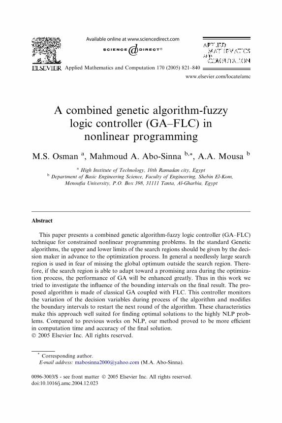
Any evolutionary computation technique applied to a particular problem

should address the issue of handling unfeasible individuals. In general, a search

space S consists of two disjoint subsets of feasible and unfeasible subspaces F

andU respectively. We do not make any assumptions about these subspaces; in

particular they need not be convex and they need not be connected (e.g., as it is

the case in the example in Fig. 1(Taken from [10]) where feasible part F of the

search space consist of two disjoined subsets).The general nonlinear programming problem for continuous variables [1] is

to find �x so as to

Min f ð�xÞ;�x ¼ ðx1; . . . ; xnÞ 2 Rn; ð1ÞWhere �x 2 F � S. The set S � Rn defines the search space and the set F � S

defines a feasible part of the search space. Usually, the search space S is defined

as n-dimensional rectangle in Rn (domains of variables defined as lower andupper bounds): left(i) 6 xi 6 right(i),1 6 i 6 n Whereas the feasible set F is

defined by the search space S and an additional set of constraints:

gjð�xÞ 6 0; for j ¼ 1; . . . . . . ;m: ð2Þ

Fig. 1. A search space and its feasible part.


Thus the nonlinear programming problem (NLPP) can be defined as follows:

NLPP: Min f ðxÞs:t: F ¼ fx 2 RnjgiðxÞ 6 0; i ¼ 1; 2; . . . ; k and hjðxÞ ¼ 0;

j ¼ k þ 1; . . . ;mgS ¼ fx 2 RnjlðxiÞ 6 xi 6 uðxiÞ; i ¼ 1; 2; . . . :; ng

ð3Þ

At any point �x 2 F, the constraint gk( Æ ) satisfy gkð�xÞ ¼ 0 are called active con-

straints at �x. By extension, equality constraints hj( Æ ) are called active at all

points of F. Nonlinear equations hj(x) = 0 requires an additional parameter

(w) to define the precision of the system [11]. All nonlinear equations

hj(x) = 0 (for j = k + 1, . . . ,m) are replaced by pair of inequalities:

�w 6 hj(x) 6 w so we deal only with nonlinear inequalities.

NLPP: Min f ðxÞs:t: F ¼ fx 2 RnjgiðxÞ 6 0; i ¼ 1; 2; . . . ;mg

S ¼ fx 2 RnjlðxiÞ 6 xi 6 uðxiÞ; i ¼ 1; 2; . . . :; ngð4Þ

3. Genetic algorithms (GAs)

GA, invented by Holland in the early 1970s, as a stochastic global search

method that mimics the metaphor of natural biological evaluation. GAs oper-

ates on a population of candidate solutions encoded to finite bit string called

chromosome. In order to obtain optimality, each chromosome exchangesinformation by using operators borrowed from natural genetic to produce

the better solution. GAs differ from other optimization and search procedures

in four ways[14]:

(1) GAs work with a coding of the parameter set, not the parameters them-

selves. Therefore GAs can easily handle the integer or discrete variables.

(2) GAs search from a population of points, not a single point. Therefore GAs

can provide a globally optimal solution.(3) GAs use only objective function information, not derivatives or other aux-

iliary knowledge. Therefore GAs can deal with the non-smooth, non-con-

tinuous and non-differentiable functions which are actually existed in a

practical optimization problem.

(4) GAs use probabilistic transition rules, not deterministic rules.

In this section we describes the main features of Modified Co-Evolutionary

Genetic Algorithm (M-COGA)[15]. The main idea behind this algorithm is


based on the ideas of co-evolution and repair algorithms (repair unfeasible

solution).

It combines concept of co-evolution, repairing procedure (Repairing unfea-

sible solution) and elitist strategy. Repairing procedure, repairs the unfeasible

points to satisfy the feasible space F. Elitist strategy is used to produce a faster

convergence of the algorithm to the optimal solution of the problem. Theworking procedure of M-COGA is described in the following manner:

3.1. Solution representation

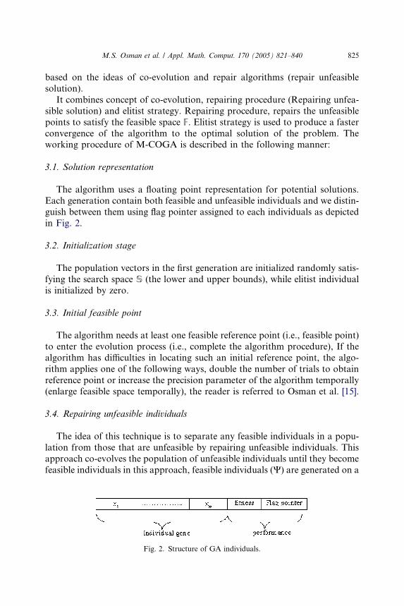
The algorithm uses a floating point representation for potential solutions.

Each generation contain both feasible and unfeasible individuals and we distin-

guish between them using flag pointer assigned to each individuals as depicted

in Fig. 2.

3.2. Initialization stage

The population vectors in the first generation are initialized randomly satis-

fying the search space S (the lower and upper bounds), while elitist individual

is initialized by zero.

3.3. Initial feasible point

The algorithm needs at least one feasible reference point (i.e., feasible point)

to enter the evolution process (i.e., complete the algorithm procedure), If the

algorithm has difficulties in locating such an initial reference point, the algo-

rithm applies one of the following ways, double the number of trials to obtain

reference point or increase the precision parameter of the algorithm temporally

(enlarge feasible space temporally), the reader is referred to Osman et al. [15].

3.4. Repairing unfeasible individuals

The idea of this technique is to separate any feasible individuals in a popu-

lation from those that are unfeasible by repairing unfeasible individuals. This

approach co-evolves the population of unfeasible individuals until they become

feasible individuals in this approach, feasible individuals (W) are generated on a

Fig. 2. Structure of GA individuals.


segment defined by two points, reference point nðtÞ 2 F and any unfeasible

individual (x).

3.5. Elitist strategy

Using an elitist strategy to produce a faster convergence of the algorithm tothe optimal solution of the problem. The elitist individual represents the more

fit point of the population. The use of elitist individual guarantees that the best

fitness individual never increase (Minimization Problem) from one generation

to the next generation (Towards the end of the process).

3.6. Evolution process stage

The algorithm uses the objective function to evaluate fitness functions foreach individual. The algorithm applies tournament selection procedure/roulette

wheel selection to select the new population.

3.7. Stopping rule

The algorithm is terminated for either one of the following conditions is

satisfied:

• The maximum number of generations is achieved.

• When the genotypes (the genotypes structures) of the population of individ-

uals converges, convergence of the genotype structure occur when all bit

positions in all strings are identical. In this case, crossover will have no fur-

ther effect.

The algorithm procedures are shown in Fig. 3 (taken from [12]).

Some of the problems with the implementation of the genetic algorithms aretheir limited accuracy of the final solution and the high number of function

evaluation required to obtain the solution, thus we tried to investigate the influ-

ence of the bounding intervals on the final result by using FLC.

4. Fuzzy logic controller

The concept of fuzzy logic was first introduced in 1960�s by Professor LoftiZadeh [18]. Fuzzy logic allows the programmer to deal with natural, ‘‘linguistic

sets’’ of states, such as very hot, warm, cold, freezing, etc. The application of

fuzzy logic involves three steps: fuzzification, rule evaluation, and defuzzifica-

tion. Fuzzification is the process of taking actual real-world data such as tem-

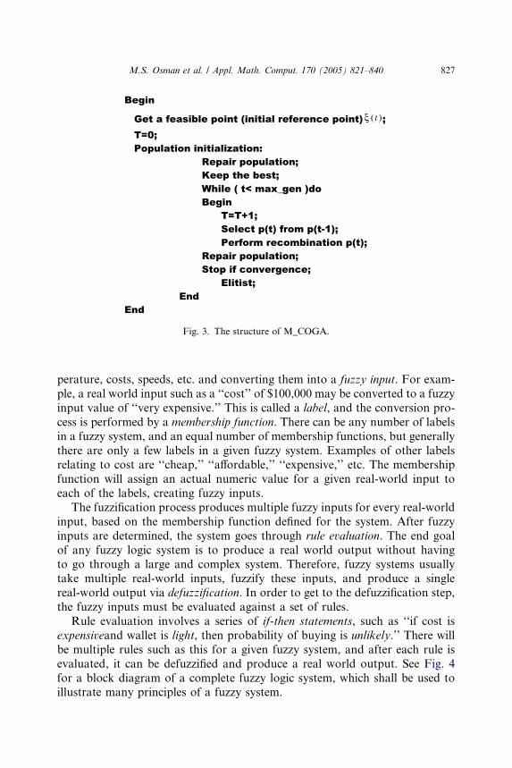
Begin

Get a feasible point (initial reference point) ( ) tξ ; T=0; Population initialization:

Repair population;Keep the best;While ( t< max_gen )doBegin T=T+1; Select p(t) from p(t-1);

Perform recombination p(t);Repair population;Stop if convergence; Elitist;

EndEnd

Fig. 3. The structure of M_COGA.


perature, costs, speeds, etc. and converting them into a fuzzy input. For exam-

ple, a real world input such as a ‘‘cost’’ of $100,000 may be converted to a fuzzy

input value of ‘‘very expensive.’’ This is called a label, and the conversion pro-

cess is performed by a membership function. There can be any number of labels

in a fuzzy system, and an equal number of membership functions, but generally

there are only a few labels in a given fuzzy system. Examples of other labelsrelating to cost are ‘‘cheap,’’ ‘‘affordable,’’ ‘‘expensive,’’ etc. The membership

function will assign an actual numeric value for a given real-world input to

each of the labels, creating fuzzy inputs.

The fuzzification process produces multiple fuzzy inputs for every real-world

input, based on the membership function defined for the system. After fuzzy

inputs are determined, the system goes through rule evaluation. The end goal

of any fuzzy logic system is to produce a real world output without having

to go through a large and complex system. Therefore, fuzzy systems usuallytake multiple real-world inputs, fuzzify these inputs, and produce a single

real-world output via defuzzification. In order to get to the defuzzification step,

the fuzzy inputs must be evaluated against a set of rules.

Rule evaluation involves a series of if-then statements, such as ‘‘if cost is

expensiveand wallet is light, then probability of buying is unlikely.’’ There will

be multiple rules such as this for a given fuzzy system, and after each rule is

evaluated, it can be defuzzified and produce a real world output. See Fig. 4

for a block diagram of a complete fuzzy logic system, which shall be used toillustrate many principles of a fuzzy system.

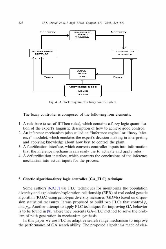
Fig. 4. A block diagram of a fuzzy control system.


The fuzzy controller is composed of the following four elements:

1. A rule-base (a set of If-Then rules), which contains a fuzzy logic quantifica-

tion of the expert�s linguistic description of how to achieve good control.

2. An inference mechanism (also called an ‘‘inference engine’’ or ‘‘fuzzy infer-

ence’’ module), which emulates the expert�s decision making in interpreting

and applying knowledge about how best to control the plant.3. A fuzzification interface, which converts controller inputs into information

that the inference mechanism can easily use to activate and apply rules.

4. A defuzzification interface, which converts the conclusions of the inference

mechanism into actual inputs for the process.

5. Genetic algorithm-fuzzy logic controller (GA_FLC) technique

Some authors [6,9,17] use FLC techniques for monitoring the population

diversity and exploitation/exploration relationship (EER) of real coded genetic

algorithm (RGA) using genotypic diversity measures (GDMs) based on disper-

sion statistical measures. It was proposed to build two FLCs that control pcand pm. Another attempt to apply FLC techniques for improving GA behavior

is to be found in [8], where they presents GA–FLC method to solve the prob-

lem of path generation in mechanism synthesis.In this paper we use FLC as adaptive search range mechanism to improve

the performance of GA search ability. The proposed algorithms made of clas-


sical GA based on the ideas of repair algorithms coupled with FLC technique.

Fuzzy logic controller controls the boundary intervals during the process of the

algorithm. This controller takes advantages of the way each variable evolves

during the optimization and adjusts the bounding intervals so that the next

run of the optimization yields a better result.

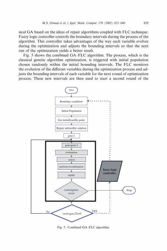
Fig. 5 shows the combined GA–FLC algorithm. The process, which is theclassical genetic algorithm optimization, is triggered with initial population

chosen randomly within the initial bounding intervals. The FLC monitors

the evolution of the different variables during the optimization process and ad-

justs the bounding intervals of each variable for the next round of optimization

process. These new intervals are then used to start a second round of the

Start

Boundary condition

Initial Population

Get initialfeasible point

Repair unfeasible solution

select

perform recombination

repair

mod (gen,25)=0

evaluation

convergenceoccur

gen=1

gen=gen+1

YESNo

Stop

fuzzy logic controller

Fig. 5. Combined GA–FLC algorithm.


algorithm. By analyzing the final result after each round, a parameter JV is

determined and the bounding interval for each variable is corrected using the

following criteria [8]:

x�l ¼ xave � JV =2ðxu � xlÞ;x�u ¼ xave þ JV =2ðxu � xlÞ:

ð5Þ

Where xave is the average value of the variable x of all the individuals of the last

generation and [xu,xl] is the bounding interval of the variable x.

The coefficient JV (the output variable) is obtained from the knowledge of

the two input variables ED and CV, where ED is the criteria for measuring

the diversity of the real coded genetic algorithm we propose one of these mea-

sures, which is based on the Euclidean distances of the chromosomes in thepopulation from the best one. It is denoted as ED.

ED ¼�d� dmin

dmax � dmin

ð6Þ

where �d ¼ 1N

PNi¼1dðCbest;CiÞ; dmax ¼ maxfdðCbest;CiÞjCi 2 Pg and dmin =

min {d(Cbest,Ci)jCi 2 P}, P denotes the population. The range of ED is [0,1].

If ED is low, most chromosomes in the population are concentrated around

the best chromosome and so convergence is achieved. If ED is high most chro-mosome are not biased toward the current best element and CV is a counter of

the variation of each parameter during each round of the algorithm. Experi-

mentally, we found that 25 generation is the best size of each round, so every

25 generation, we modifies the boundary condition for each variable depending

on the knowledge of the two input ED and CV found during the last round of

the algorithm. Consequently, CV is a counter for each one of the variables and

it is ranging between 0 and 25. It starts at 0 and during the last 25 generations it

is incremented by 1 each time the variable changes. Therefore, CV could bethought of as an indicator of the number of times the variable changes during

this round of the algorithm. A low indicator means that the variable is very

close to its optimum and we do not need to change the initial bounding inter-

val. A high indicator requires the adjustment of the initial bounding interval to

improve the final solution. This adjustment is conditioned also by the accuracy

of the obtained solution. Indeed if we reach an accurate solution in the first

round of GA there is no need to perform any change even if we get high indi-

cators for some variables. This reasoning is best implemented using a fuzzylogic controller.

5.1. Fuzzification

Fuzzification of the input variables is the first step in the design of a fuzzy

logic controller. Fuzzification of the input variables involves quantizing the uni-

verses into a number of fuzzy sets. The output variables also need to be quan-


tized in a similar manner. Quantization involves breaking up a fuzzy input (and

also output) variable into several fuzzy subsets. Linguistic variables are used to

label the fuzzy subsets (Table 1) so that the rules can be written in a natural lan-

guage form. For simplicity we can choose the same (triangular) membership

functions for each of the fuzzy subsets of all the fuzzy variables. Fig. 6 shows

the membership functions chosen for the 2 fuzzy input variables and the outputvariable and Table 2 contains the definition of the linguistic parameters.

5.2. The knowledge base

The knowledge base of a fuzzy logic controller consists of a data base and a

rule base. The basic function of the data base is to provide the necessary infor-

mation for the proper functioning of the fuzzification module, the rule base and

the defuzzification module. The rules are as follows: IF condition AND condi-

tion THEN conclusion. For simplification a matrix can be used for presenting

the rules which is called the fuzzy rule matrix. Table 2 shows the fuzzy rule ma-

trix used by the inference mechanism.

Control signals have been generated by the controller basing on the rules

base presented above. Fuzzy logic toolbox prepared control surface, which is

presented in Fig. 7.

5.3. Defuzzification

Defuzzification is a mapping from a space of fuzzy control actions defined

over an output universe of discourse into a space of non-fuzzy (crisp) control

action. The defuzzification method used in the algorithm is the center of gravity

method. This procedure is the most prevalent and physically appealing of all

the defuzzification methods. Fig. 6 shows the membership functions of the out-

put variables.

6. Experimental verification

To validate our proposed algorithm, we present three problems solved on a

Pentium III 900 MHz and implemented in MATLAB 6.5.

Table 1

The linguistic variables

VS Very small

S Small

M Medium

H High

VH Very High

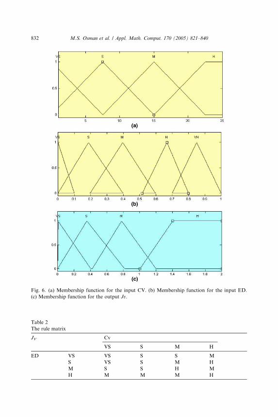
Fig. 6. (a) Membership function for the input CV. (b) Membership function for the input ED.

(c) Membership function for the output Jv.

Table 2

The rule matrix

JV Cv

VS S M H

ED VS VS S S M

S VS S M H

M S S H M

H M M M H


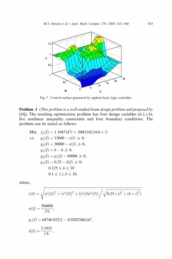
Fig. 7. Control surface generated by applied fuzzy logic controller.


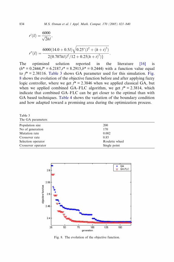
Problem 1 (This problem is a well-studied beam design problem and proposed by

[16]). The resulting optimization problem has four design variables (h, l, t,b),

five nonlinear inequality constraints and four boundary conditions. The

problem can be stated as follows:

Min fwð~xÞ ¼ 1:10471h2lþ :04811tbð14:0þ lÞs:t: g1ð~xÞ ¼ 13600� rð~xÞ P 0;

g2ð~xÞ ¼ 30000� rð~xÞ P 0;

g3ð~xÞ ¼ b� h P 0;

g4ð~xÞ ¼ pcð~xÞ � 60000 P 0;

g5ð~xÞ ¼ 0:25� dð~xÞ P 0;

0:125 6 h 6 10

0:1 6 l; t; b 6 10;

where,

rð~xÞ ¼

ffiffiffiffiffiffiffiffiffiffiffiffiffiffiffiffiffiffiffiffiffiffiffiffiffiffiffiffiffiffiffiffiffiffiffiffiffiffiffiffiffiffiffiffiffiffiffiffiffiffiffiffiffiffiffiffiffiffiffiffiffiffiffiffiffiffiffiffiffiffiffiffiffiffiffiffiffiffiffiffiffiffiffiffiffiffiffiffiffiffiffiffiffiffiffiffiffiffiffiffiffiffiffiffiffiffiffiffiffiffiffiffiffiffiffiffiffiðr0ð~xÞÞ2 þ ðr00ð~xÞÞ2 þ lðr0ð~xÞr00ð~xÞÞ

� ffiffiffiffiffiffiffiffiffiffiffiffiffiffiffiffiffiffiffiffiffiffiffiffiffiffiffiffiffiffiffiffiffiffiffiffiffiffiffiffiffiffi0:25 � ðl2 þ ðhþ tÞ2Þ

qs

rð~xÞ ¼ 504000

t2b;

pcð~xÞ ¼ 64746:022ð1� 0:0282346tÞtb3;

dð~xÞ ¼ 2:1952

t3b;


r0ð~xÞ ¼ 6000ffiffiffi2

phl

;

r00ð~xÞ ¼6000ð14:0þ 0:5lÞ

ffiffiffiffiffiffiffiffiffiffiffiffiffiffiffiffiffiffiffiffiffiffiffiffiffiffiffiffiffiffiffiffiffiffiffiffiffiffiffi0:25�ðl2 þ ðhþ tÞ2Þ

q2f0:707hlðl2=12þ 0:25ðhþ tÞ2Þg

:

The optimized solution reported in the literature [16] is

(h* = 0.2444,l* = 6.2187,t* = 8.2915,b* = 0.2444) with a function value equal

to f* = 2.38116. Table 3 shows GA parameter used for this simulation. Fig.

8 shows the evolution of the objective function before and after applying fuzzy

logic controller, where we get f* = 2.3846 when we applied classical GA, but

when we applied combined GA–FLC algorithm, we get f* = 2.3814, whichindicate that combined GA–FLC can be get closer to the optimal than with

GA based techniques. Table 4 shows the variation of the boundary condition

and how adapted toward a promising area during the optimization process.

Table 3

The GA parameters

Population size 200

No of generation 170

Mutation rate 0.002

Crossover rate 0.85

Selection operator Roulette wheel

Crossover operator Single point

Fig. 8. The evolution of the objective function.

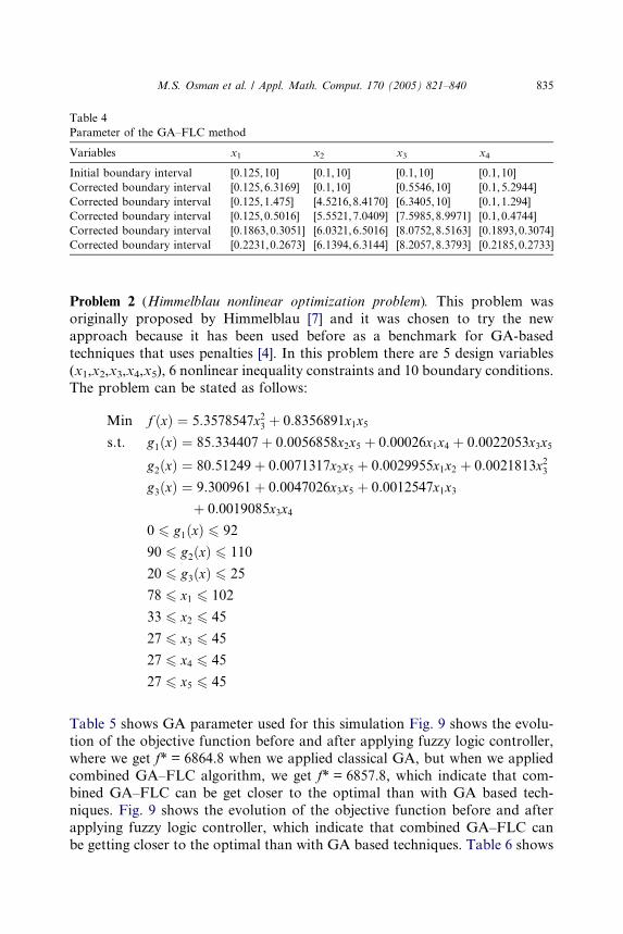
Table 4

Parameter of the GA–FLC method

Variables x1 x2 x3 x4

Initial boundary interval [0.125,10] [0.1,10] [0.1,10] [0.1,10]

Corrected boundary interval [0.125,6.3169] [0.1,10] [0.5546,10] [0.1,5.2944]

Corrected boundary interval [0.125,1.475] [4.5216,8.4170] [6.3405,10] [0.1,1.294]

Corrected boundary interval [0.125,0.5016] [5.5521,7.0409] [7.5985,8.9971] [0.1,0.4744]




Problem 2 (Himmelblau nonlinear optimization problem). This problem was

originally proposed by Himmelblau [7] and it was chosen to try the new

approach because it has been used before as a benchmark for GA-based

techniques that uses penalties [4]. In this problem there are 5 design variables

(x1,x2,x3,x4,x5), 6 nonlinear inequality constraints and 10 boundary conditions.

The problem can be stated as follows:

Min f ðxÞ ¼ 5:3578547x23 þ 0:8356891x1x5s:t: g1ðxÞ ¼ 85:334407þ 0:0056858x2x5 þ 0:00026x1x4 þ 0:0022053x3x5

g2ðxÞ ¼ 80:51249þ 0:0071317x2x5 þ 0:0029955x1x2 þ 0:0021813x23g3ðxÞ ¼ 9:300961þ 0:0047026x3x5 þ 0:0012547x1x3

þ 0:0019085x3x40 6 g1ðxÞ 6 92

90 6 g2ðxÞ 6 110

20 6 g3ðxÞ 6 25

78 6 x1 6 102

33 6 x2 6 45

27 6 x3 6 45

27 6 x4 6 45

27 6 x5 6 45

Table 5 shows GA parameter used for this simulation Fig. 9 shows the evolu-

tion of the objective function before and after applying fuzzy logic controller,

where we get f* = 6864.8 when we applied classical GA, but when we applied

combined GA–FLC algorithm, we get f* = 6857.8, which indicate that com-bined GA–FLC can be get closer to the optimal than with GA based tech-

niques. Fig. 9 shows the evolution of the objective function before and after

applying fuzzy logic controller, which indicate that combined GA–FLC can

be getting closer to the optimal than with GA based techniques. Table 6 shows

Table 5

The GA parameters

Population size 179


Mutation rate 0.002

Crossover rate 0.85




Table 6


Variables x1 x2 x3 x4 x5

Initial boundary

interval

[78,102] [33,45] [27,45] [27,45] [27,45]

Corrected boundary

interval

[78,83.3257] [33,35.5430] [27,31.1171] [41.3654,45] [40.4699,45]

Corrected boundary

interval

[78,79.0947] [33,33.5964] [27,27.9941] [44.2702,45] [43.8118,45]

Corrected boundary

interval

[78,78.2233] [33,33.17] [27,27.3319] [44.8605,45] [44.5532,44.9935]

Corrected boundary

interval

[78,78.0573] [33,33.0604] [27.0396,27.1706] [44.9666,45] [44.8047,44.9785]

Corrected boundary

interval

[78,78.0180] [33,33.0253] [27.0539,27.1063] [44.9925,45] [44.9126,44.9817]



the variation of the boundary condition and how adapted toward a promising

area during the optimization process.

Problem 3. This problem was solved by Michalewicz [13] by different

constraint handling techniques. The optimized solution reported in [13] is~x = (2.171996,2.363683,8.773926,5.959840,0.990654,1.430574,1.321644,9.828726,8.280092,8.375927), f * = 24.306209. In this problem there are 10 design

variables (x1,x2,x3,x4,x5,x6,x7,x8,x9,x10), 8 nonlinear inequality constraints

The first six constraints are active at this solution. The problem can be stated as

follows:

Min f ðxÞ ¼ x21 þ x22 þ x1x2 � 14x1 � 16x2 þ ðx3 � 10Þ2

þ 4ðx4 � 5Þ2 þ ðx5 � 3Þ2 þ 2ðx6 � 1Þ2 þ 5x27

þ 7ðx8 � 11Þ2 þ 2ðx9 � 11Þ2 þ ðx10 � 7Þ2 þ 45;

s:t: g1ðxÞ ¼ 105� 4x1 � 5x2 þ 3x7 � 9x8 P 0;

g2ðxÞ ¼ �10x1 þ 8x2 þ 17x7 � 2x8 P 0;

g3ðxÞ ¼ 8x1 � 2x2 þ 5x9 þ 2x10 þ 12 P 0;

g4ðxÞ ¼ �3ðx1 � 2Þ2 � 4ðx2 � 3Þ2 � 2x23 þ 7x4 þ 120 P 0;

g5ðxÞ ¼ �5x21 � 8x2 � ðx3 � 6Þ2 þ 2x4 þ 40 P 0;

g6ðxÞ ¼ �x21 � 2ðx2 � 2Þ2 þ 2x1x2 � 14x5 þ 6x6 P 0;

g7ðxÞ ¼ �0:5ðx1 � 8Þ2 � 2ðx2 � 4Þ2 � 3x25 þ x6 þ 30 P 0;

g8ðxÞ ¼ 3x1 � 6x2 � 12ðx9 � 8Þ2 þ 7x0 P 0;

� 10 6 xi 6 10; i ¼ 1; . . . 10:

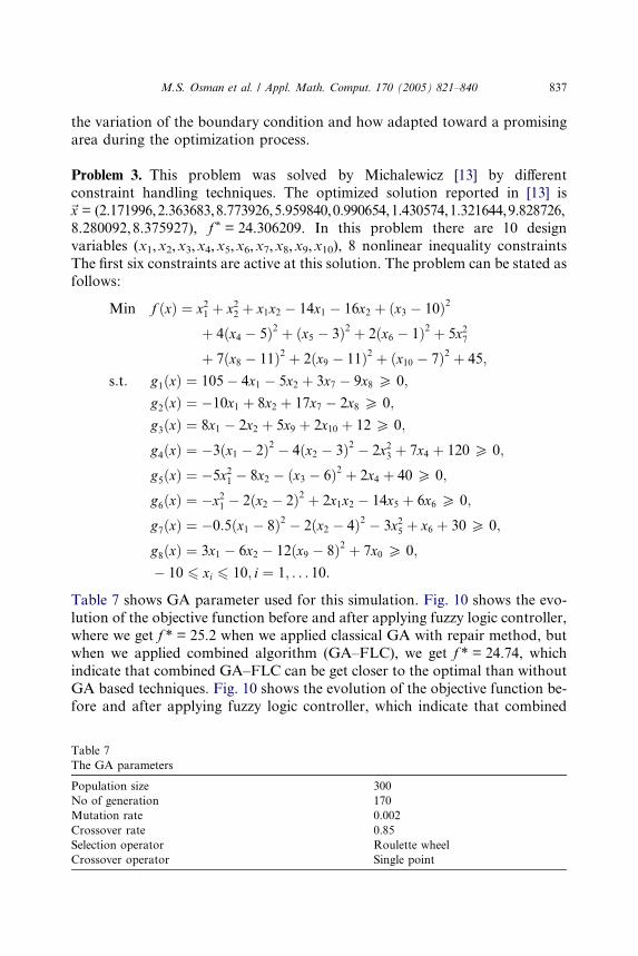
Table 7 shows GA parameter used for this simulation. Fig. 10 shows the evo-

lution of the objective function before and after applying fuzzy logic controller,

where we get f * = 25.2 when we applied classical GA with repair method, but

when we applied combined algorithm (GA–FLC), we get f * = 24.74, which

indicate that combined GA–FLC can be get closer to the optimal than without

GA based techniques. Fig. 10 shows the evolution of the objective function be-

fore and after applying fuzzy logic controller, which indicate that combined

Table 7

The GA parameters

Population size 300


Mutation rate 0.002

Crossover rate 0.85





GA–FLC can be get closer to the optimal than with GA based techniques.Table 8 shows the variation of the boundary condition for the initial round

of GA and the boundary condition for the successive rounds of GA and

how adapted toward a promising area during the optimization process.

7. Conclusion

This paper presents a combined genetic algorithm fuzzy logic controllertechniques (GA–FLC) to solve constrained NLP problems. This algorithm is

made of a classical genetic algorithm based on the ideas of repair method cou-

pled with a fuzzy logic controller, This fuzzy logic controller monitors the var-

iation of the decision variables during the process of GA and changes the initial

boundary condition to start the next round of The algorithm to get closer to

the promising area of the search space. We showed through experimental result

that the obtained result is always better than classical GA.

Comparing to previous work on constrained NLP problems, our approachproved to be more efficient than classical GA in finding optimal solution. The

search space are shrunk with highly rate to the optimal solution region through

the process of the algorithm. So the process converges rapidly to the final solu-

tion. Also, the proposed algorithm allowed us to get closer to the target than

the genetic algorithm based techniques. In brief, this algorithm has capability

to adjust its starting population to avoid local minimum and to obtain accura-

cies that classical GA fail to obtain. Several examples allowed us to compare

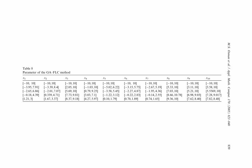
Table 8


x1 x2 x3 x4 x5 x6 x7 x8 x9 x10

[�10, 10] [�10,10] [�10,10] [�10,10] [�10,10] [�10, 10] [�10,10] [�10,10] [�10,10] [�10,10]

[�3.95,7.91] [�3.39,8.4] [2.05,10] [�1.03,10] [�5.02,6.22] [�3.15,5.75] [�2.67,5.19] [5.33,10] [3.11,10] [3.58,10]

[�2.65,6.86] [�2.01,7.07] [5.69,10] [0.79,9.25] [�3.58,5.45] [�2.27,4.87] [�1.95,4.36] [7.03,10] [5.21,10] [5.5569,10]

[�0.18,4.39] [0.339,4.71] [7.73,9.81] [3.03,7.1] [�1.22,3.12] [�0.22,2.83] [�0.14,2.55] [8.66,10.78] [6.98,9.03] [7.28,9.017]

[1.21,3] [1.67,3.37] [8.37,9.18] [4.27,5.97] [0.10,1.79] [0.70,1.89] [0.74,1.65] [9.36,10] [7.62,8.40] [7.82,8.48]

M.S.Osm

anet

al./Appl.Math.Comput.170(2005)821–840

839


our results with those found in the literature. The numerical analysis shows

that our combined algorithm turns out to be very efficient in computation time

and accuracy of the final solution.

References

[1] M.S. Bazaraa, Nonlinear Programming: Theory and Algorithms, John Willy & Sons, New

York, 1979.

[2] C. Coello, Treating constraints as objectives for single-objective evolutionary optimization,

Engineering Optimization 32 (3) (2000) 275–308.

[3] K. Deb, Optimal design of a welded beam structure via genetic algorithms, ALAA journal

29/11 (1991) 2013–2015.

[4] M. Gen, R. Cheng, Genetic Algorithms & Engineering Design, John Wiley & Sons Inc, New

York, 1997.

[5] D.E. Goldberg, Genetic Algorithms in Search, Optimization and Machine Learning, Addison

Wesley Publishing Company, 1989.

[6] F. Herrera, E. Herrera-Viedma, M. Lozano, J.L. Verdegay, Fuzzy tools to improve genetic

algorithms, in: proc. second European Congress on Intelligent Techniques and Soft

Computing 1532–1539 (1994).

[7] D.M. Himmmeblau, Applied Nonlinear Programming, McGraw-Hill, New York, 1972.

[8] M.A. Laribi, A. Mlika, L. Romdhane, S. Zeghloul, A combined genetic algorithm-fuzzy logic

method (GA_FL) in mechanisms synthesis, Mechanism And Machine Theory 39 (2004) 717–

735.

[9] M.A. Lee, H. Takagi, Dynamic control of genetic algorithms using fuzzy logic techniques, in:

S. Forrest, (Ed.), proc. of the fifth Int. Conf. on Genetic Algorithms Morgan Kaufmmann, San

Mateo, (1993) 76–83.

[10] Z. Michalewicz, A survey of constraint handling techniques in evolutionary computation

methods, proceeding of the 4th Annual Conference on Evolutionary Programming, MIT

Press, Cambridge, MA, (1995) 135–155.

[11] Z. Michalewicz, Schoenauer, Evolutionary algorithms for constrained parameter optimization

problems, Evolutionary Computation 4 (1) (1996) 1–32.

[12] Z. Michalewicz, G. Nazhiyath, Genocop III: A Co-evolutionary Algorithm for Numerical

Optimization Problems and with nonlinear constraints, in: D.B. Fogel (Ed.), Proceedings of

the Second IEEE International Conference on Evolutionary Computation, IEEE press, 1995,

pp. 647–651.

[13] Z. Michalewicz, Genetic Algorithms, Numerical Optimization, and Constraints, in: L.

Eshelman (Ed.), Proceedings of The Sixth International Conference on Genetic Algorithms,

Morgan Kauffman, San Mateo, 1995, pp. 151–158.

[14] Z. Michalewicz, Genetic Algorithms + Data Structures = Volution Programs, third ed.,

Springer-Verlag, 1996.

[15] M.S. Osman, M.A. Abo-Sinna, A.A. Mousa, A solution to the optimal power flow using

genetic algorithm, Applied Mathematics and Computation 155 (2004) 391–405.

[16] G.V. Reklaitis, A. Ravindran, K.M. Ragsdell, Engineering Optimization Methods and

Applications, Wiley, New York, 1983.

[17] P.T. Wang, G.S. Wang, Z.G. Hu, Speeding Up The Search Process of Genetic Algorithm by

Fuzzy Logic, in: proc. 5th European Congress on Intelligent Techniques and Soft Computing,

1997, pp. 665–671.

[18] L.A. Zadeh, Fuzzy Sets, Information and Control 8 (3) (1965) 338–353.

A combined genetic algorithm-fuzzy logic controller (GA-FLC) in nonlinear programming

Documents