A Classification-based Approach to Manage a Solver Portfolio for CSPs

A Classification-based Approach to Manage a SolverPortfolio for CSPs

Zeynep Kiziltan Luca Mandrioli Jacopo MauroBarry O’Sullivan

Technical Report UBLCS-2012-01

Jan 2012

Department of Computer ScienceUniversity of Bologna

Mura Anteo Zamboni 740126 Bologna (Italy)

A Classification-based Approach to Manage a SolverPortfolio for CSPs

Zeynep Kiziltan 1 Luca Mandrioli1 Jacopo Mauro1 Barry O’Sullivan2

Technical Report UBLCS-2012-01

Jan 2012

Abstract

The utility of using portfolios of solvers for constraint satisfaction problems is well reported. We show thatwhen runtimes are properly clustered, simple classification techniques can be used to predict the class ofruntime as, for example, short, medium, long, time-out, etc. Based on runtime classifiers we demonstrate adispatching approach to solve a set of problem instances in order to minimize the average completion timeof each instance. We show that this approach significantly out-performs a well-known CSP solver andperforms well against an oracle implementation of a solver portfolio.

1. Computer Science Department, University of Bologna, Italy2. Cork Constraint Computation Centre, University College Cork, Ireland

1

1 Introduction

1 IntroductionThe past decade has witnessed a significant increase in the number of constraint solving systemsdeployed for solving constraint satisfaction problems (CSP). It is well recognized within the fieldof constraint programming that different solvers are better at solving different problem instances,even within the same problem class [3]. It has been shown in other areas, such as satisfiabilitytesting [19] and integer linear programming [8], that the best on-average solver can be out per-formed by a portfolio of possibly slower on-average solvers. This selection process is usuallyperformed using a machine learning technique based on feature data extracted from CSPs.

Three specific approaches that use contrasting approaches to portfolio management inCSP, SAT and QBF are CPHYDRA, SATZILLA, and ACME, respectively. CPHYDRA is a portfo-lio of constraint solvers exploiting a case-base of problem solving experience [12]. CPHYDRAcombines case-base reasoning of machine learning with the idea of partitioning CPU-TIME be-tween components of the portfolio in order to maximize the expected number of solved probleminstances within a fixed time limit. SATZILLA [19] builds runtime prediction models using linearregression techniques based on structural features computed from instances of Boolean satisfi-ability problem. Given an unseen instance of the satisfiability problem, SATZILLA selects thesolver from its portfolio that it predicts to have the fastest running time on the instance. TheACME system is a portfolio approach to solve quantified Boolean formulae, i.e. SAT instanceswith some universally quantified variables [13].

In this paper we present a very different approach to managing a portfolio for constraintsolving when the objective is to solve a set of problem instances so that the average completiontime, i.e. the time at which we have either found a solution or proven that none exist, of eachinstance is minimized. This scenario arises in a context in which problem instances are submit-ted to, for example, a cloud-based solver which queues and solves instances in an autonomousfashion. This scenario is consistent with our long term objective which is to build an on-lineservice-based portfolio solver that receives CSPs from a user to solve, exploits multiple process-ing nodes to search for solutions and returns the answer as quickly as possible (see [7] for moredetails). In addition, there is a significant scheduling literature that focuses on minimizing aver-age completion time, much of which is based around the use of dispatching heuristics [17].

The approach we propose in this paper is strongly inspired by dispatching rules for schedul-ing. Our approach is conceptually simple, but powerful. Specifically, we propose the use of clas-sifier techniques as a basis for making high-level and qualitative statements about the solvabilityof CSP instances with respect to a given solver portfolio. We also use classifier techniques as abasis for a dispatching-like approach to solve a set of problem instances in a single processor sce-nario. We show that when runtimes are properly clustered, simple classification techniques canbe used to predict the class of runtime as, for example, short, medium, long, time-out, etc. Weshow that this approach significantly out-performs a well-known general-purpose CSP solverand performs well against an oracle implementation of a portfolio.

The remainder of this paper is organized as follows. In Section 2 we summarize the requi-site background on constraint satisfaction and machine learning required for this paper. Section 3presents the large collection of CSP instances on which we base our study. We discuss the variousclassification tasks upon which our approach is based in Section 4, and evaluate the suitability ofdifferent representations and classification for these tasks in Section 5. We demonstrate the util-ity of our classification-based approach for managing a solver portfolio in Section 6. We discussrelated work in Section 7 and conclude in Section 8.

2 PreliminariesA constraint satisfaction problem (CSP) is defined by a finite set of variables, each associated with adomain of possible values that the variable can be assigned, and a set of constraints that define theset of allowed assignments of values to the variables [9]. The arity of a constraint is the numberof variables it constrains. Given a CSP, the task is normally to find an assignment to the variablesthat satisfies the constraints, which we refer to as a solution.

UBLCS-2012-01 2

3 The International CSP Competition Dataset

Machine learning “is concerned with the question of how to construct computer programs thatautomatically improve with experience”. It is a broad field that uses concepts from computer science,mathematics, statistics, information theory, complexity theory, biology and cognitive science [10].Machine learning can be applied to well-defined problems, where there is both a source of train-ing examples and one or more metrics for measuring performance. In this paper we are partic-ularly interested in classification tasks. A classifier is a function that maps an instance with oneor more discrete or continuous features to one of a finite number of classes [10]. A classifier istrained on a set of instances whose class is already known, with the intention that the classifiercan transfer its training experiences to the task of classifying new instances.

3 The International CSP Competition DatasetWe focused on demonstrating our approach on as comprehensive and a realistic set of prob-lem instances as possible. Therefore, we constructed a comprehensive dataset of CSPs based onthe various instances gathered for the annual International CSP Solver Competition3 from 2006-2008. An advantage of using these instances is that they are publicly available in a standard-ized XML-based format called XCSP.4 The first competition was held in 2005, and all benchmarkproblems were represented using extensional constraints only. In 2006, both intentional and ex-tensional constraints were used. In 2008, global constraints were also added. Overall, there arefive categories of benchmark problem in the competition: 2-ARY-EXT instances involving extension-ally defined binary (and unary) constraints; N-ARY-EXT instances involving extensionally definedconstraints, at least one of which is defined over more than two variables; 2-ARY-INT instancesinvolving intensionally defined binary (and unary) constraints; N-ARY-INT instances involvingintensionally defined constraints, at least one of which is defined over more than two variables;and, GLB instances involving any kind of constraints, including global constraints.

The competition required that any instance should be solved within 1800 seconds. Anyinstance not solved by this cut-off time was considered unsolved. To facilitate our analysis, weremove from the dataset any instance that could not have been solved by any of the solvers of ourportfolio by the cut-off. In total, our data set contains around 4000 instances across these variouscategories.

4 From Runtime Clustering to Runtime ClassificationWe show how clusters of runtimes can be used to define classification problems for a dispatching-based approach to managing an algorithm portfolio. While our focus here is not to develop theCPHYDRA system, we will, for convenience, use its constituent solvers and feature descriptionsof problem instances to build our classifiers. We demonstrate our approach on a comprehensiveand realistic set of problem instances.

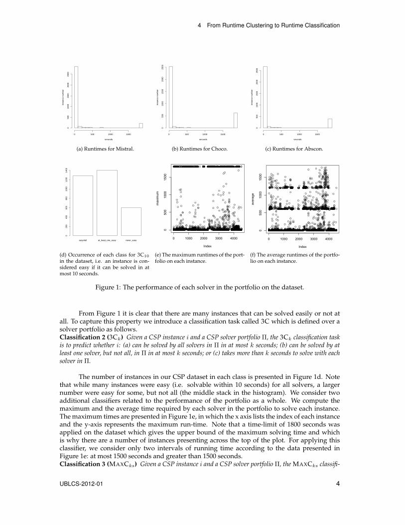
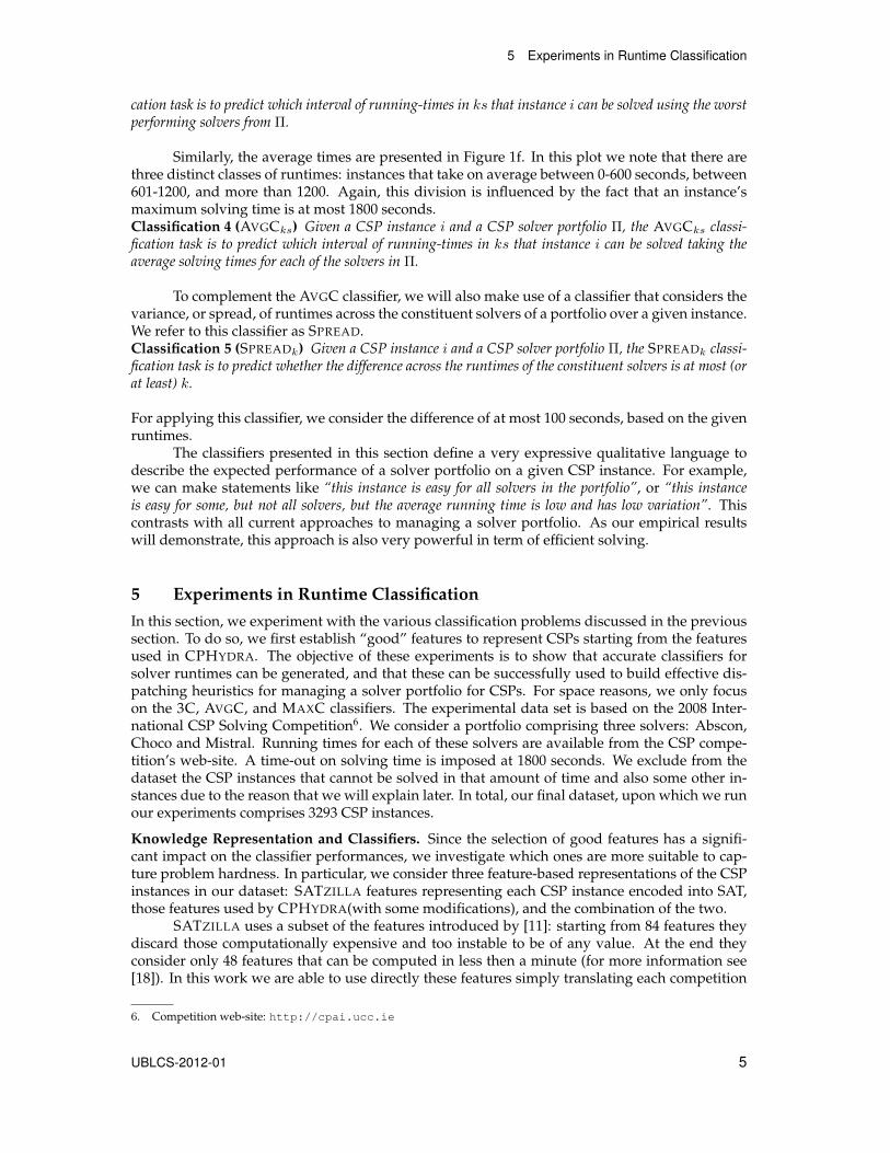
Based on the three solvers used in the 2008 CSP Solver Competition variant of CPHYDRAwe present in Figures 1a, 1b, and 1c the runtime distributions for each of its solvers, Mistral,Choco, and Abscon respectively,5 showing for every solver in the portfolio the number of in-stances of the data set solved in given time windows. Having removed from the dataset anyinstance that could not have been solved by any of these solvers within a 1800s time-limit, eachinstance is ensured to be solved by at least one solver. However, it is not the case that each solverfinds that the same instances are either easy or hard. There are many instances, as we will showbelow, for which one of the solvers decides the instance quickly, while another solver strugglesto solve it. Therefore we define a classification task that given a CSP instance returns the fastestsolver for that instance.Classification 1 (Fastest Solver Classification (FS)) Given a CSP instance i and a CSP solver portfo-lio Π, the FS classification task is to predict which solver in Π gives the fastest runtime on i.

3. Competition web-site: http://cpai.ucc.ie4. http://www.cril.univ-artois.fr/˜lecoutre/benchmarks.html5. Visit the competition site for links to each of the solvers.

UBLCS-2012-01 3

4 From Runtime Clustering to Runtime Classification

seconds

inst

ance

num

ber

0 500 1000 1500

050

010

0015

0020

0025

00

(a) Runtimes for Mistral.

seconds

inst

ance

num

ber

0 500 1000 1500

050

010

0015

0020

0025

00

(b) Runtimes for Choco.

seconds

inst

ance

num

ber

0 500 1000 1500

050

010

0015

0020

0025

00

(c) Runtimes for Abscon.

easy4all at_least_one_easy never_easy

020

040

060

080

010

0012

0014

00

(d) Occurrence of each class for 3C10

in the dataset, i.e. an instance is con-sidered easy if it can be solved in atmost 10 seconds.

0 1000 2000 3000 4000

0500

1000

1500

Index

maximum

(e) The maximum runtimes of the port-folio on each instance.

0 1000 2000 3000 4000

0500

1000

1500

Index

average

(f) The average runtimes of the portfo-lio on each instance.

Figure 1: The performance of each solver in the portfolio on the dataset.

From Figure 1 it is clear that there are many instances that can be solved easily or not atall. To capture this property we introduce a classification task called 3C which is defined over asolver portfolio as follows.Classification 2 (3Ck) Given a CSP instance i and a CSP solver portfolio Π, the 3Ck classification taskis to predict whether i: (a) can be solved by all solvers in Π in at most k seconds; (b) can be solved by atleast one solver, but not all, in Π in at most k seconds; or (c) takes more than k seconds to solve with eachsolver in Π.

The number of instances in our CSP dataset in each class is presented in Figure 1d. Notethat while many instances were easy (i.e. solvable within 10 seconds) for all solvers, a largernumber were easy for some, but not all (the middle stack in the histogram). We consider twoadditional classifiers related to the performance of the portfolio as a whole. We compute themaximum and the average time required by each solver in the portfolio to solve each instance.The maximum times are presented in Figure 1e, in which the x axis lists the index of each instanceand the y-axis represents the maximum run-time. Note that a time-limit of 1800 seconds wasapplied on the dataset which gives the upper bound of the maximum solving time and whichis why there are a number of instances presenting across the top of the plot. For applying thisclassifier, we consider only two intervals of running time according to the data presented inFigure 1e: at most 1500 seconds and greater than 1500 seconds.Classification 3 (MAXCks) Given a CSP instance i and a CSP solver portfolio Π, the MAXCks classifi-

UBLCS-2012-01 4

5 Experiments in Runtime Classification

cation task is to predict which interval of running-times in ks that instance i can be solved using the worstperforming solvers from Π.

Similarly, the average times are presented in Figure 1f. In this plot we note that there arethree distinct classes of runtimes: instances that take on average between 0-600 seconds, between601-1200, and more than 1200. Again, this division is influenced by the fact that an instance’smaximum solving time is at most 1800 seconds.Classification 4 (AVGCks) Given a CSP instance i and a CSP solver portfolio Π, the AVGCks classi-fication task is to predict which interval of running-times in ks that instance i can be solved taking theaverage solving times for each of the solvers in Π.

To complement the AVGC classifier, we will also make use of a classifier that considers thevariance, or spread, of runtimes across the constituent solvers of a portfolio over a given instance.We refer to this classifier as SPREAD.Classification 5 (SPREADk) Given a CSP instance i and a CSP solver portfolio Π, the SPREADk classi-fication task is to predict whether the difference across the runtimes of the constituent solvers is at most (orat least) k.

For applying this classifier, we consider the difference of at most 100 seconds, based on the givenruntimes.

The classifiers presented in this section define a very expressive qualitative language todescribe the expected performance of a solver portfolio on a given CSP instance. For example,we can make statements like “this instance is easy for all solvers in the portfolio”, or “this instanceis easy for some, but not all solvers, but the average running time is low and has low variation”. Thiscontrasts with all current approaches to managing a solver portfolio. As our empirical resultswill demonstrate, this approach is also very powerful in term of efficient solving.

5 Experiments in Runtime ClassificationIn this section, we experiment with the various classification problems discussed in the previoussection. To do so, we first establish “good” features to represent CSPs starting from the featuresused in CPHYDRA. The objective of these experiments is to show that accurate classifiers forsolver runtimes can be generated, and that these can be successfully used to build effective dis-patching heuristics for managing a solver portfolio for CSPs. For space reasons, we only focuson the 3C, AVGC, and MAXC classifiers. The experimental data set is based on the 2008 Inter-national CSP Solving Competition6. We consider a portfolio comprising three solvers: Abscon,Choco and Mistral. Running times for each of these solvers are available from the CSP compe-tition’s web-site. A time-out on solving time is imposed at 1800 seconds. We exclude from thedataset the CSP instances that cannot be solved in that amount of time and also some other in-stances due to the reason that we will explain later. In total, our final dataset, upon which we runour experiments comprises 3293 CSP instances.

Knowledge Representation and Classifiers. Since the selection of good features has a signifi-cant impact on the classifier performances, we investigate which ones are more suitable to cap-ture problem hardness. In particular, we consider three feature-based representations of the CSPinstances in our dataset: SATZILLA features representing each CSP instance encoded into SAT,those features used by CPHYDRA(with some modifications), and the combination of the two.

SATZILLA uses a subset of the features introduced by [11]: starting from 84 features theydiscard those computationally expensive and too instable to be of any value. At the end theyconsider only 48 features that can be computed in less then a minute (for more information see[18]). In this work we are able to use directly these features simply translating each competition

6. Competition web-site: http://cpai.ucc.ie

UBLCS-2012-01 5

5 Experiments in Runtime Classification

CSP instance into SAT using the Sugar solver7 and then using SATZILLA to extract its feature de-scription. In some (but few) cases, the encoding of a CSP instance into SAT requires an excessiveamount of time (i.e. more than a day). In order to make a fair comparison between the set offeatures, we simply dropped such instances from the dataset.

For the second feature representation, we started from the 36 features of CPHYDRA. Whilstthe majority of them are syntactical, the remaining are computed by collecting data from shortruns of the Mistral solver. Among the syntactical features, worth mentioning are the number ofvariables, the number of constraints and global constraints, the number of constants, the sizes ofthe domains and the arity of the predicates. The dynamic features instead take into account thenumber of nodes explored and the number of propagations done by Mistral with a time limit of2 seconds. When we extracted the CPHYDRA features using our dataset we noticed that two ofthem (viz. the logarithm of the number of constants and the logarithm of the number of extravalues) were constant. Since constant features are not useful for discriminating between differentproblems, we discarded these two features. Inspired by Nudelman et al [11], we consideredadditional features like the ratio of the number constraints over the number variables, and theratio of the number of variables over the number of constraints. Moreover, we added featuresrepresenting an instance’s variable graph and variable-constraint graph. In the former, each variableis represented by a node with an edge between pairs of nodes if they occur together in at leastone constraint. In the latter, we construct a bipartite graph in which each variable and constraintis represented by a node, with an edge between a variable node v and a constraint node c if v isconstrained by c. From these graphs, we extract the average and standard deviation of the nodedegrees and take their logarithm. With these, the total amount of features we consider are 42.

The third feature-based description of the CSP instances, which we refer to as HYLLA, issimply the concatenation of the two feature descriptions discussed above. We consider a varietyof classifiers, implemented in publicly available tools RapidMiner8 and WEKA.9 Our SVM classi-fier is hand-tuned to the specific tasks considered in this paper according to the best parametersfound using RapidMiner; however, it is only applied to the 3C and AVGC tasks because it ap-peared to be problematic to tune for the MAXC task. The other WEKA classifiers are used withtheir default settings.

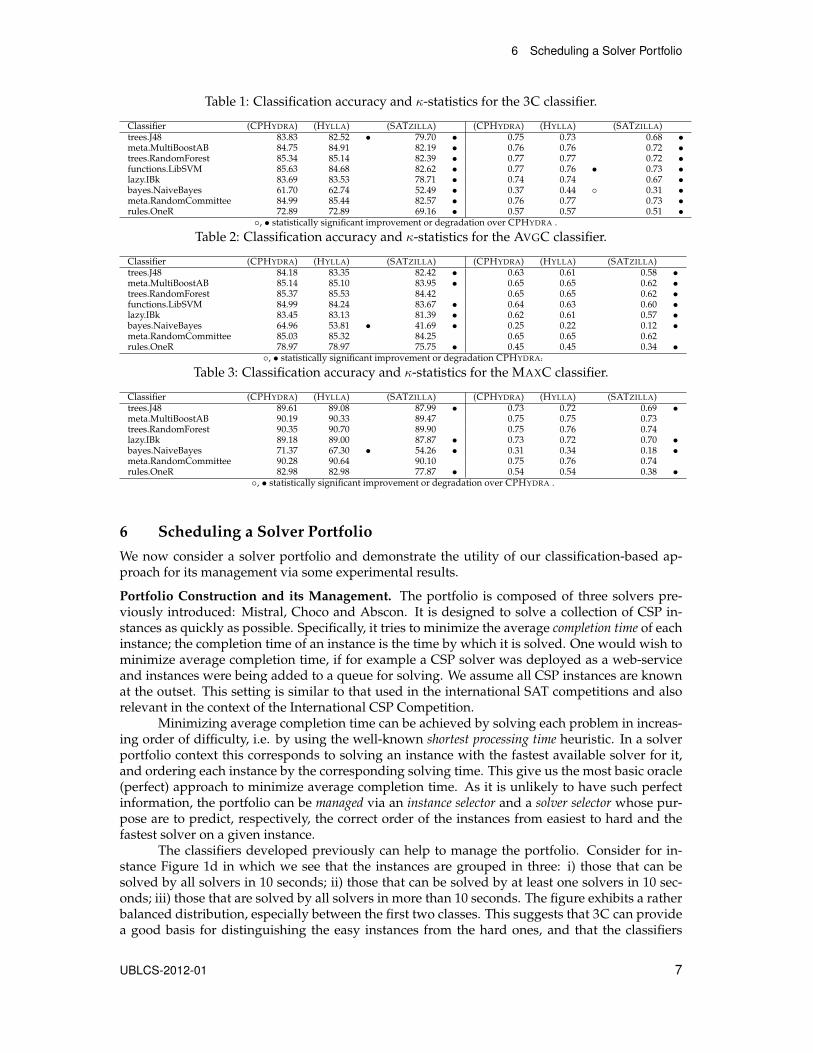
Results. The results of the runtime classification tasks are presented in Tables 1– 3. Three alter-native feature descriptions, as discussed earlier, are compared; these are denoted as CPHYDRA,HYLLA, and SATZILLA, in the tables. We compare the performance of various classifiers on eachof the three classification tasks (3C, MAXC, and AVGC). A 10-fold cross-validation is performed.The performance of each classifier, on each representation, on each classification task are mea-sured in terms of the classification accuracy and the κ-statistic. The latter measures the relativeimprovement in classification over a random predictor.

Differences in performance are tested for statistical significance using a Paired t-Test at a95% confidence level. The performance on the CPHYDRA feature set is used as a baseline. In eachtable, values that are marked with a ◦ represent performances that are statistically significantlybetter than CPHYDRA, while those marked with a • represent performances that are statisticallysignificantly worse.

In summary, both classification accuracies and κ values are high across all three tasks.Interestingly, combining both CPHYDRA and SATZILLA features improves performance in onlyone κ value, and without any significant improvement in classification accuracy. The CPHYDRAfeature set thus gives rise to the best overall performance. Based on these promising results, weconsider in the next section the utility of using these classifiers as a basis for managing how asolver portfolio can be used to solve a collection of CSP instances.

7. http://bach.istc.kobe-u.ac.jp/sugar/8. http://rapid-i.com/content/view/181/196/9. http://www.cs.waikato.ac.nz/ml/weka/

UBLCS-2012-01 6

6 Scheduling a Solver Portfolio

Table 1: Classification accuracy and κ-statistics for the 3C classifier.

Classifier (CPHYDRA) (HYLLA) (SATZILLA) (CPHYDRA) (HYLLA) (SATZILLA)trees.J48 83.83 82.52 • 79.70 • 0.75 0.73 0.68 •meta.MultiBoostAB 84.75 84.91 82.19 • 0.76 0.76 0.72 •trees.RandomForest 85.34 85.14 82.39 • 0.77 0.77 0.72 •functions.LibSVM 85.63 84.68 82.62 • 0.77 0.76 • 0.73 •lazy.IBk 83.69 83.53 78.71 • 0.74 0.74 0.67 •bayes.NaiveBayes 61.70 62.74 52.49 • 0.37 0.44 ◦ 0.31 •meta.RandomCommittee 84.99 85.44 82.57 • 0.76 0.77 0.73 •rules.OneR 72.89 72.89 69.16 • 0.57 0.57 0.51 •

◦, • statistically significant improvement or degradation over CPHYDRA .

Table 2: Classification accuracy and κ-statistics for the AVGC classifier.

Classifier (CPHYDRA) (HYLLA) (SATZILLA) (CPHYDRA) (HYLLA) (SATZILLA)trees.J48 84.18 83.35 82.42 • 0.63 0.61 0.58 •meta.MultiBoostAB 85.14 85.10 83.95 • 0.65 0.65 0.62 •trees.RandomForest 85.37 85.53 84.42 0.65 0.65 0.62 •functions.LibSVM 84.99 84.24 83.67 • 0.64 0.63 0.60 •lazy.IBk 83.45 83.13 81.39 • 0.62 0.61 0.57 •bayes.NaiveBayes 64.96 53.81 • 41.69 • 0.25 0.22 0.12 •meta.RandomCommittee 85.03 85.32 84.25 0.65 0.65 0.62rules.OneR 78.97 78.97 75.75 • 0.45 0.45 0.34 •

◦, • statistically significant improvement or degradation CPHYDRA.

Table 3: Classification accuracy and κ-statistics for the MAXC classifier.

Classifier (CPHYDRA) (HYLLA) (SATZILLA) (CPHYDRA) (HYLLA) (SATZILLA)trees.J48 89.61 89.08 87.99 • 0.73 0.72 0.69 •meta.MultiBoostAB 90.19 90.33 89.47 0.75 0.75 0.73trees.RandomForest 90.35 90.70 89.90 0.75 0.76 0.74lazy.IBk 89.18 89.00 87.87 • 0.73 0.72 0.70 •bayes.NaiveBayes 71.37 67.30 • 54.26 • 0.31 0.34 0.18 •meta.RandomCommittee 90.28 90.64 90.10 0.75 0.76 0.74rules.OneR 82.98 82.98 77.87 • 0.54 0.54 0.38 •

◦, • statistically significant improvement or degradation over CPHYDRA .

6 Scheduling a Solver PortfolioWe now consider a solver portfolio and demonstrate the utility of our classification-based ap-proach for its management via some experimental results.

Portfolio Construction and its Management. The portfolio is composed of three solvers pre-viously introduced: Mistral, Choco and Abscon. It is designed to solve a collection of CSP in-stances as quickly as possible. Specifically, it tries to minimize the average completion time of eachinstance; the completion time of an instance is the time by which it is solved. One would wish tominimize average completion time, if for example a CSP solver was deployed as a web-serviceand instances were being added to a queue for solving. We assume all CSP instances are knownat the outset. This setting is similar to that used in the international SAT competitions and alsorelevant in the context of the International CSP Competition.

Minimizing average completion time can be achieved by solving each problem in increas-ing order of difficulty, i.e. by using the well-known shortest processing time heuristic. In a solverportfolio context this corresponds to solving an instance with the fastest available solver for it,and ordering each instance by the corresponding solving time. This give us the most basic oracle(perfect) approach to minimize average completion time. As it is unlikely to have such perfectinformation, the portfolio can be managed via an instance selector and a solver selector whose pur-pose are to predict, respectively, the correct order of the instances from easiest to hard and thefastest solver on a given instance.

The classifiers developed previously can help to manage the portfolio. Consider for in-stance Figure 1d in which we see that the instances are grouped in three: i) those that can besolved by all solvers in 10 seconds; ii) those that can be solved by at least one solvers in 10 sec-onds; iii) those that are solved by all solvers in more than 10 seconds. The figure exhibits a ratherbalanced distribution, especially between the first two classes. This suggests that 3C can providea good basis for distinguishing the easy instances from the hard ones, and that the classifiers

UBLCS-2012-01 7

6 Scheduling a Solver Portfolio

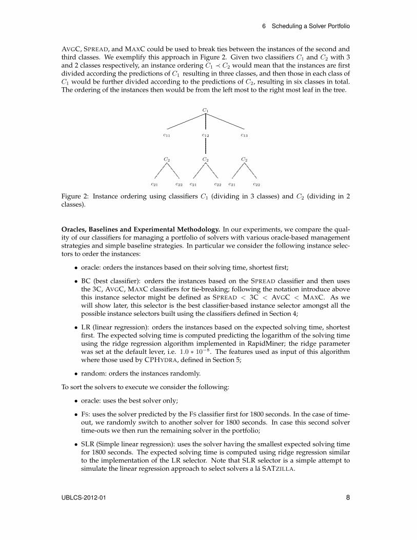
AVGC, SPREAD, and MAXC could be used to break ties between the instances of the second andthird classes. We exemplify this approach in Figure 2. Given two classifiers C1 and C2 with 3and 2 classes respectively, an instance ordering C1 ≺ C2 would mean that the instances are firstdivided according the predictions of C1 resulting in three classes, and then those in each class ofC1 would be further divided according to the predictions of C2, resulting in six classes in total.The ordering of the instances then would be from the left most to the right most leaf in the tree.

C1

c13

C2

c22c21

c12

C2

c22c21

c11

C2

c22c21

Figure 2: Instance ordering using classifiers C1 (dividing in 3 classes) and C2 (dividing in 2classes).

Oracles, Baselines and Experimental Methodology. In our experiments, we compare the qual-ity of our classifiers for managing a portfolio of solvers with various oracle-based managementstrategies and simple baseline strategies. In particular we consider the following instance selec-tors to order the instances:

• oracle: orders the instances based on their solving time, shortest first;

• BC (best classifier): orders the instances based on the SPREAD classifier and then usesthe 3C, AVGC, MAXC classifiers for tie-breaking; following the notation introduce abovethis instance selector might be defined as SPREAD < 3C < AVGC < MAXC. As wewill show later, this selector is the best classifier-based instance selector amongst all thepossible instance selectors built using the classifiers defined in Section 4;

• LR (linear regression): orders the instances based on the expected solving time, shortestfirst. The expected solving time is computed predicting the logarithm of the solving timeusing the ridge regression algorithm implemented in RapidMiner; the ridge parameterwas set at the default lever, i.e. 1.0 ∗ 10−8. The features used as input of this algorithmwhere those used by CPHYDRA, defined in Section 5;

• random: orders the instances randomly.

To sort the solvers to execute we consider the following:

• oracle: uses the best solver only;

• FS: uses the solver predicted by the FS classifier first for 1800 seconds. In the case of time-out, we randomly switch to another solver for 1800 seconds. In case this second solvertime-outs we then run the remaining solver in the portfolio;

• SLR (Simple linear regression): uses the solver having the smallest expected solving timefor 1800 seconds. The expected solving time is computed using ridge regression similarto the implementation of the LR selector. Note that SLR selector is a simple attempt tosimulate the linear regression approach to select solvers a la SATZILLA.

UBLCS-2012-01 8

6 Scheduling a Solver Portfolio

• SLR+: which uses first the solver having the smallest expected solving time for 1800 sec-onds. In case of time-out, we switch to the solver having the second smallest expectedsolving time. This solver is run for 1800 seconds and, in case it time-outs, we run theremaining solver in the portfolio. The expected solving time is computed using ridge re-gression similar to the implementation of the LR selector;

• CPHYDRA: simulates the performance that would be obtained from CPHYDRA10. Thesolver scheduling algorithm of CPHYDRA is used to partition the time window of 1800seconds among the three solver of the portfolio. We then simulate what would have hap-pened if Mistral was used first, Choco for second and Abscon for last; 11

• Mistral: uses only Mistral for 1800 seconds;

• Random: tries the solvers in a sequence in random order, every one of them with a timeoutof 1800 seconds.

As noted earlier, our benchmarks are composed of instances that can be solved by at leastone solver by the cut-off. Whilst the SLR, CPHYDRA, and Mistral solver selectors do not guar-antee that all instances will be solved, all the other selector can make such a claim. In particularMistral is not able to solve 7.871% of instances whilst using the SLR and CPHYDRA solver selec-tors 3.83% and 0.91% of the instances were not solved, respectively.

In the experiments, we adopt a simple random split validation approach to evaluate thequality of our classifiers for managing a portfolio of solvers. We use the instances described inSection 3. Given a management strategy, we execute it (via simulation) 1000 times. A single runconsists in random split of the dataset into a testing set (1/5 of the instances) and a training set(the remaining 4/5). We use the random forest algorithm (RapidMiner) for learning the mod-els. For every run, we compute the overall average solving times and report just the average ofthe average solving times across 1000 runs. Differences in performance are tested for statisticalsignificance using a Paired t-test at a 95% confidence level.

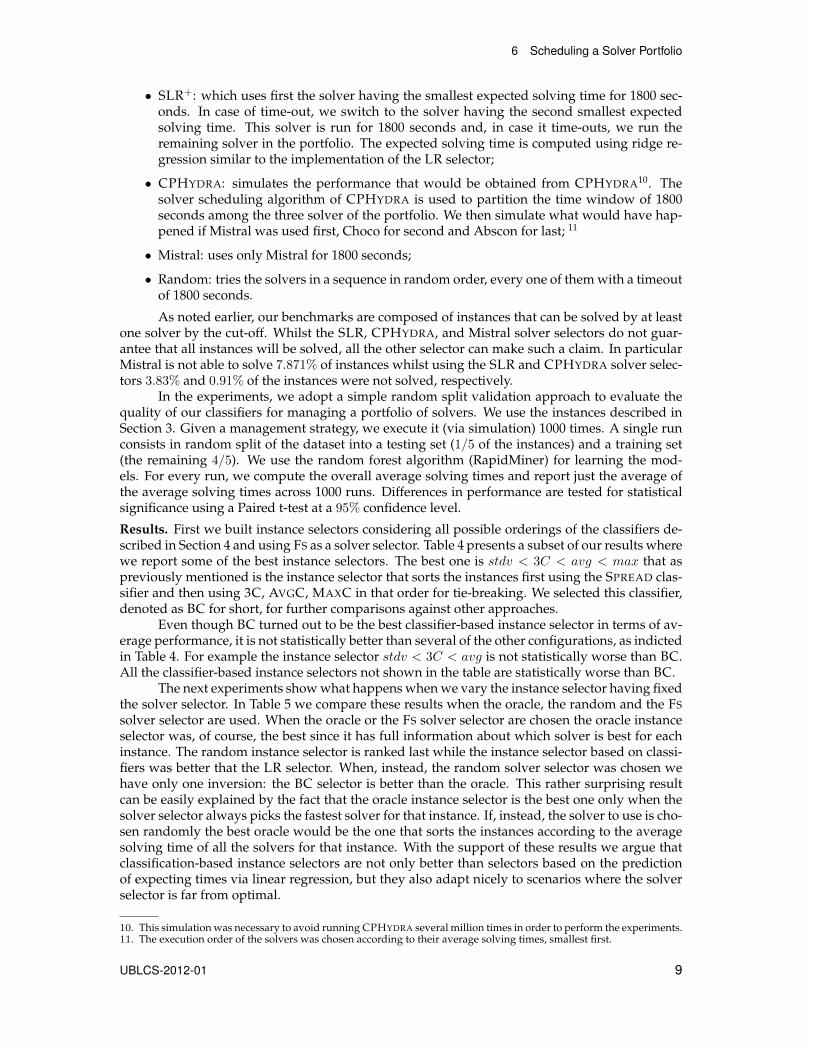
Results. First we built instance selectors considering all possible orderings of the classifiers de-scribed in Section 4 and using FS as a solver selector. Table 4 presents a subset of our results wherewe report some of the best instance selectors. The best one is stdv < 3C < avg < max that aspreviously mentioned is the instance selector that sorts the instances first using the SPREAD clas-sifier and then using 3C, AVGC, MAXC in that order for tie-breaking. We selected this classifier,denoted as BC for short, for further comparisons against other approaches.

Even though BC turned out to be the best classifier-based instance selector in terms of av-erage performance, it is not statistically better than several of the other configurations, as indictedin Table 4. For example the instance selector stdv < 3C < avg is not statistically worse than BC.All the classifier-based instance selectors not shown in the table are statistically worse than BC.

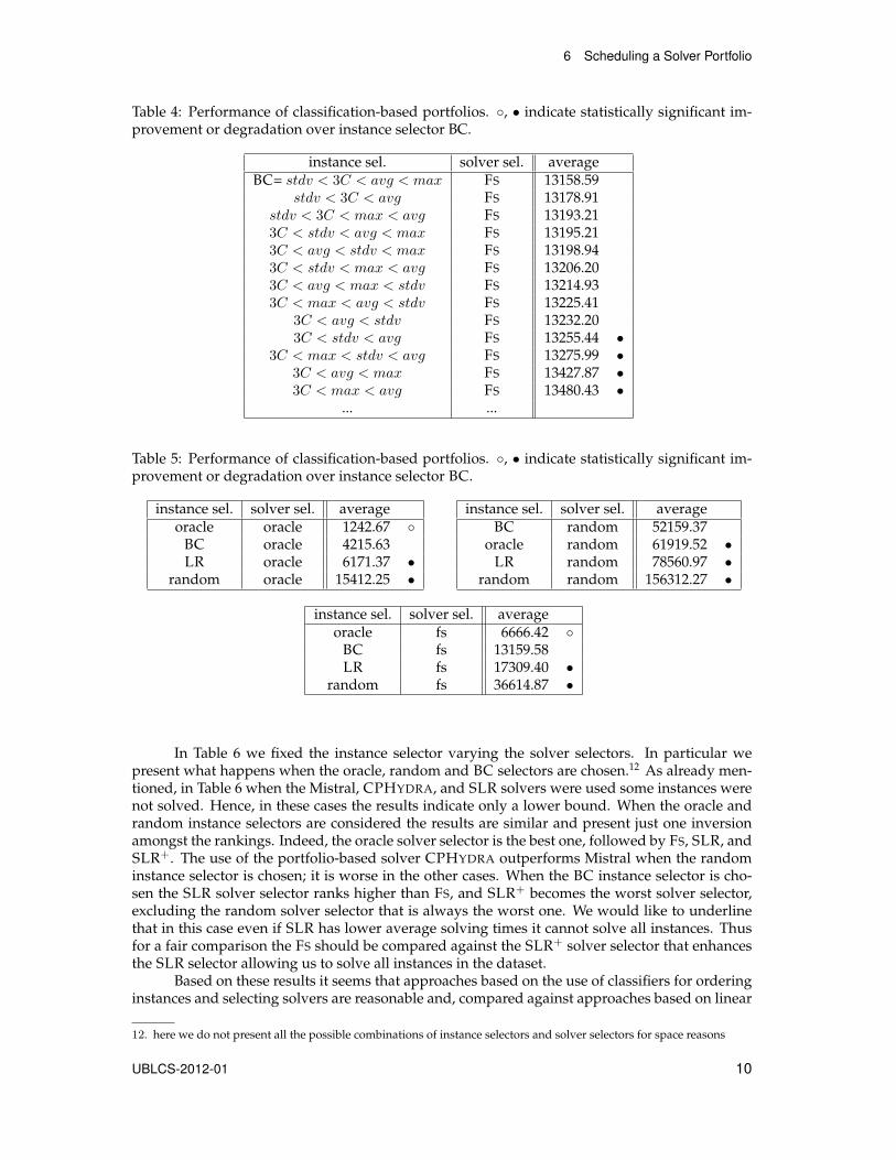
The next experiments show what happens when we vary the instance selector having fixedthe solver selector. In Table 5 we compare these results when the oracle, the random and the FSsolver selector are used. When the oracle or the FS solver selector are chosen the oracle instanceselector was, of course, the best since it has full information about which solver is best for eachinstance. The random instance selector is ranked last while the instance selector based on classi-fiers was better that the LR selector. When, instead, the random solver selector was chosen wehave only one inversion: the BC selector is better than the oracle. This rather surprising resultcan be easily explained by the fact that the oracle instance selector is the best one only when thesolver selector always picks the fastest solver for that instance. If, instead, the solver to use is cho-sen randomly the best oracle would be the one that sorts the instances according to the averagesolving time of all the solvers for that instance. With the support of these results we argue thatclassification-based instance selectors are not only better than selectors based on the predictionof expecting times via linear regression, but they also adapt nicely to scenarios where the solverselector is far from optimal.

10. This simulation was necessary to avoid running CPHYDRA several million times in order to perform the experiments.11. The execution order of the solvers was chosen according to their average solving times, smallest first.

UBLCS-2012-01 9

6 Scheduling a Solver Portfolio

Table 4: Performance of classification-based portfolios. ◦, • indicate statistically significant im-provement or degradation over instance selector BC.

instance sel. solver sel. averageBC= stdv < 3C < avg < max FS 13158.59

stdv < 3C < avg FS 13178.91stdv < 3C < max < avg FS 13193.213C < stdv < avg < max FS 13195.213C < avg < stdv < max FS 13198.943C < stdv < max < avg FS 13206.203C < avg < max < stdv FS 13214.933C < max < avg < stdv FS 13225.41

3C < avg < stdv FS 13232.203C < stdv < avg FS 13255.44 •

3C < max < stdv < avg FS 13275.99 •3C < avg < max FS 13427.87 •3C < max < avg FS 13480.43 •

... ...

Table 5: Performance of classification-based portfolios. ◦, • indicate statistically significant im-provement or degradation over instance selector BC.

instance sel. solver sel. averageoracle oracle 1242.67 ◦

BC oracle 4215.63LR oracle 6171.37 •

random oracle 15412.25 •

instance sel. solver sel. averageBC random 52159.37

oracle random 61919.52 •LR random 78560.97 •

random random 156312.27 •

instance sel. solver sel. averageoracle fs 6666.42 ◦

BC fs 13159.58LR fs 17309.40 •

random fs 36614.87 •

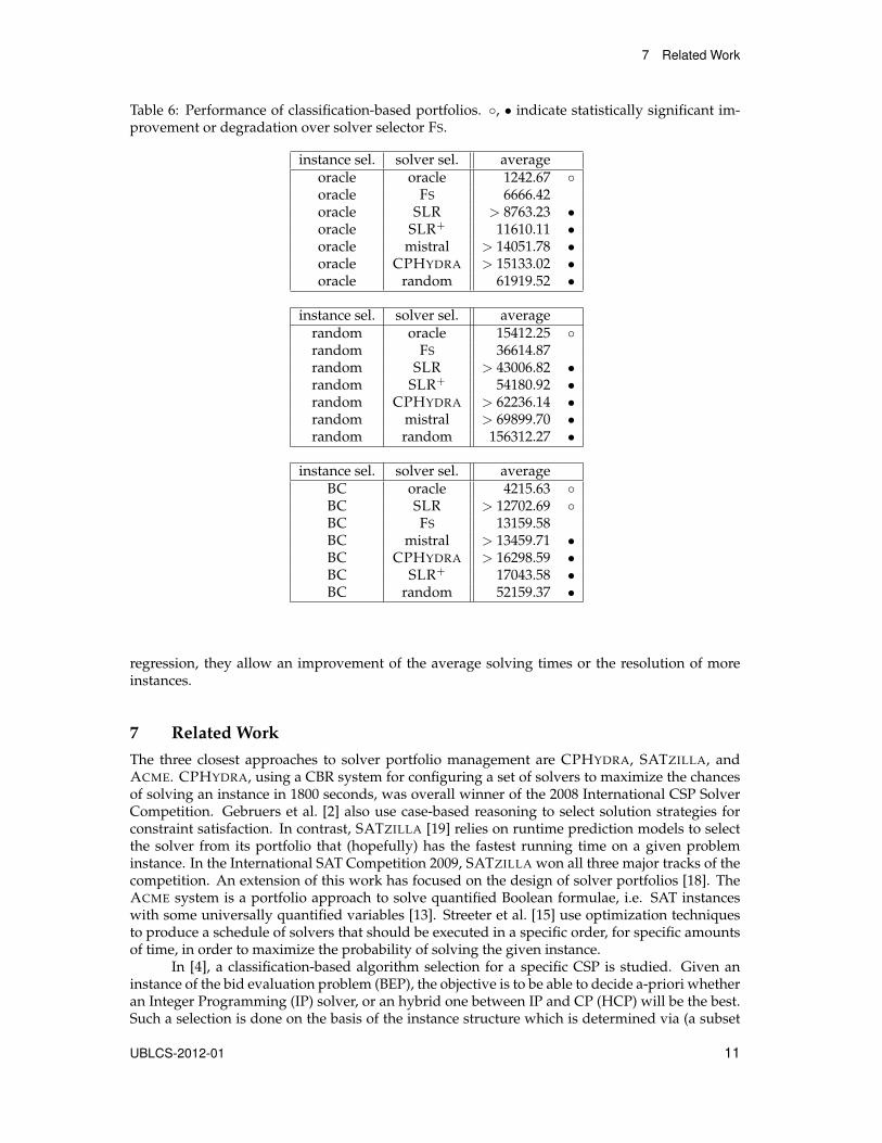
In Table 6 we fixed the instance selector varying the solver selectors. In particular wepresent what happens when the oracle, random and BC selectors are chosen.12 As already men-tioned, in Table 6 when the Mistral, CPHYDRA, and SLR solvers were used some instances werenot solved. Hence, in these cases the results indicate only a lower bound. When the oracle andrandom instance selectors are considered the results are similar and present just one inversionamongst the rankings. Indeed, the oracle solver selector is the best one, followed by FS, SLR, andSLR+. The use of the portfolio-based solver CPHYDRA outperforms Mistral when the randominstance selector is chosen; it is worse in the other cases. When the BC instance selector is cho-sen the SLR solver selector ranks higher than FS, and SLR+ becomes the worst solver selector,excluding the random solver selector that is always the worst one. We would like to underlinethat in this case even if SLR has lower average solving times it cannot solve all instances. Thusfor a fair comparison the FS should be compared against the SLR+ solver selector that enhancesthe SLR selector allowing us to solve all instances in the dataset.

Based on these results it seems that approaches based on the use of classifiers for orderinginstances and selecting solvers are reasonable and, compared against approaches based on linear

12. here we do not present all the possible combinations of instance selectors and solver selectors for space reasons

UBLCS-2012-01 10

7 Related Work

Table 6: Performance of classification-based portfolios. ◦, • indicate statistically significant im-provement or degradation over solver selector FS.

instance sel. solver sel. averageoracle oracle 1242.67 ◦oracle FS 6666.42oracle SLR > 8763.23 •oracle SLR+ 11610.11 •oracle mistral > 14051.78 •oracle CPHYDRA > 15133.02 •oracle random 61919.52 •

instance sel. solver sel. averagerandom oracle 15412.25 ◦random FS 36614.87random SLR > 43006.82 •random SLR+ 54180.92 •random CPHYDRA > 62236.14 •random mistral > 69899.70 •random random 156312.27 •

instance sel. solver sel. averageBC oracle 4215.63 ◦BC SLR > 12702.69 ◦BC FS 13159.58BC mistral > 13459.71 •BC CPHYDRA > 16298.59 •BC SLR+ 17043.58 •BC random 52159.37 •

regression, they allow an improvement of the average solving times or the resolution of moreinstances.

7 Related WorkThe three closest approaches to solver portfolio management are CPHYDRA, SATZILLA, andACME. CPHYDRA, using a CBR system for configuring a set of solvers to maximize the chancesof solving an instance in 1800 seconds, was overall winner of the 2008 International CSP SolverCompetition. Gebruers et al. [2] also use case-based reasoning to select solution strategies forconstraint satisfaction. In contrast, SATZILLA [19] relies on runtime prediction models to selectthe solver from its portfolio that (hopefully) has the fastest running time on a given probleminstance. In the International SAT Competition 2009, SATZILLA won all three major tracks of thecompetition. An extension of this work has focused on the design of solver portfolios [18]. TheACME system is a portfolio approach to solve quantified Boolean formulae, i.e. SAT instanceswith some universally quantified variables [13]. Streeter et al. [15] use optimization techniquesto produce a schedule of solvers that should be executed in a specific order, for specific amountsof time, in order to maximize the probability of solving the given instance.

In [4], a classification-based algorithm selection for a specific CSP is studied. Given aninstance of the bid evaluation problem (BEP), the objective is to be able to decide a-priori whetheran Integer Programming (IP) solver, or an hybrid one between IP and CP (HCP) will be the best.Such a selection is done on the basis of the instance structure which is determined via (a subset

UBLCS-2012-01 11

8 Conclusions

of) 25 static features derived from the constraint graph [8]. These features are extracted on a set oftraining instances and the corresponding best approach is identified. The resulting data is thengiven to a classification algorithm that builds decision trees. Our objective in this paper is notonly to be able to predict the best solver for a given instance but also to choose the right instanceat the right time to minimize the average finishing time of the set of instances. Consequently wedevelop multiple classifiers and utilize them so as to predict their order of difficulty. Moreover,our features are general-purpose and our approach works for any CSP in the XCSP format withany of the related solvers. Furthermore, we take into account a set of dynamic features whichprovide complementary information.

Also related to our work is the instance-specific algorithm configuration tool ISAC [6].Given a highly parameterized solver for a CSP instance, its purpose is to tune the parametersbased on the characteristics of the instance. Again, such characteristics are determined via staticfeatures and extracted from the training instances. Then the instances are clustered using the g-means algorithm, the best parameter tuning for each cluster is identified, and a distance thresholdis computed which determines when a new instance will be considered as close enough to thecluster to be solved with its parameters. The fundamental difference with our approach is thatinstances that are likely to prefer the same solver are grouped with a clustering algorithm basedon their features. We instead do not use any clustering algorithm. We create clusters ourselvesaccording to the observed performance of the solvers on the instances and predict which clusteran instance belongs based on its features using classification algorithms.

8 ConclusionsWe have presented a novel approach to managing a portfolio for constraint solving. We proposedthe use of classifier techniques as a basis for making high-level and qualitative statements aboutthe solvability of CSP instances with respect to a given solver portfolio. We showed how thesecould then be used for solving a collection of problem instances. While this approach is con-ceptually very simple, we demonstrated that using classifiers to develop dispatching rules for asolver portfolio is very promising.

The work presented here is a first step towards the ambitious goal of developing an on-lineservice-based portfolio solver that receives CSPs from a user, exploits multiple processing nodesto search for solutions as quickly as possible. In the future, we will study distributed strategies forsystems having more than one processor. In this setting, using more than one solver in parallelfor the same instance could also be useful. For instance, consider running all solvers in parallelfor instances that are difficult for all solvers but one, and running only the best solver for all theother instances. This strategy looks promising since it will not waste resources running all thesolvers for all the instances and, at the same time, it minimizes the risk of choosing the wrongsolver for some instances.

In this paper, our classes of run times were manually extracted. As part of future workwe consider to automate this task using clustering techniques. In addition, we will investigatethe benefit of using automatic algorithm tuning tools like GGA [1] and ParamILS [5] to train alarger portfolio of solvers. It has been observed in ISAC and Hydra that additional performancebenefits can be achieved with solvers that have been expressly tuned for a particular subset ofproblem types.

Finally we would like to exploit the solving statistics (e.g. solving times, memory con-sumption) obtained at run time to improve on-the-fly the predictions of the models. This goalhas been already considered for the QSAT domain [14]. We plan to follow similar ideas usingon-line machine learning techniques [16].

References[1] Carlos Ansotegui, Meinolf Sellmann, and Kevin Tierney. A gender-based genetic algorithm

for the automatic configuration of algorithms. In CP, pages 142–157, 2009.

UBLCS-2012-01 12

REFERENCES

[2] Cormac Gebruers, Brahim Hnich, Derek G. Bridge, and Eugene C. Freuder. Using cbr toselect solution strategies in constraint programming. In ICCBR, pages 222–236, 2005.

[3] Carla P. Gomes and Bart Selman. Algorithm portfolios. Artif. Intell., 126(1-2):43–62, 2001.

[4] Alessio Guerri and Michela Milano. Learning techniques for automatic algorithm portfolioselection. In ECAI, pages 475–479, 2004.

[5] Frank Hutter, Holger H. Hoos, Kevin Leyton-Brown, and Thomas Stutzle. Paramils: Anautomatic algorithm configuration framework. J. Artif. Intell. Res. (JAIR), 36:267–306, 2009.

[6] Serdar Kadioglu, Yuri Malitsky, Meinolf Sellmann, and Kevin Tierney. Isac - instance-specificalgorithm configuration. In ECAI, pages 751–756, 2010.

[7] Zeynep Kiziltan and Jacopo Mauro. Service-oriented volunteer computing for massivelyparallel constraint solving using portfolios. In CPAIOR, pages 246–251, 2010.

[8] Kevin Leyton-Brown, Eugene Nudelman, and Yoav Shoham. Learning the empirical hard-ness of optimization problems: The case of combinatorial auctions. In CP, pages 556–572,2002.

[9] Alan K. Mackworth. Consistency in networks of relations. Artif. Intell., 8(1):99–118, 1977.

[10] Tom M. Mitchell. Machine learning. McGraw Hill series in computer science. McGraw-Hill,1997.

[11] Eugene Nudelman, Kevin Leyton-Brown, Holger H. Hoos, Alex Devkar, and Yoav Shoham.Understanding random sat: Beyond the clauses-to-variables ratio. In CP, pages 438–452,2004.

[12] Eoin O’Mahony, Emmanuel Hebrard, Alan Holland, Conor Nugent, and Barry O’Sullivan.Using case-based reasoning in an algorithm portfolio for constraint solving. AICS 08), 2009.

[13] Luca Pulina and Armando Tacchella. A multi-engine solver for quantified boolean formulas.In CP, pages 574–589, 2007.

[14] Luca Pulina and Armando Tacchella. Time to learn or time to forget? strengths and weak-nesses of a self-adaptive approach to reasoning in quantified boolean formulas. In CP Doc-toral Program, 2008.

[15] Matthew J. Streeter, Daniel Golovin, and Stephen F. Smith. Combining multiple heuristicsonline. In AAAI, pages 1197–1203, 2007.

[16] Vladimir Vovk, Alex Gammerman, and Glenn Shafer. Algorithmic Learning in a RandomWorld. Springer-Verlag New York, Inc., Secaucus, NJ, USA, 2005.

[17] Richard J. Wallace and Eugene C. Freuder. Supporting dispatchability in schedules withconsumable resources. J. Scheduling, 8(1):7–23, 2005.

[18] Lin Xu, Holger Hoos, and Kevin Leyton-Brown. Hydra: Automatically configuring algo-rithms for portfolio-based selection. In AAAI, 2010.

[19] Lin Xu, Frank Hutter, Holger H. Hoos, and Kevin Leyton-Brown. : The design and analysisof an algorithm portfolio for sat. In CP, pages 712–727, 2007.

UBLCS-2012-01 13