A characterization of income and consumption inequality in ...

A characterization of income and consumptioninequality in Portugal

Nuno AlvesBanco de Portugal

Fátima CardosoBanco de Portugal

Nuno MonteiroBanco de Portugal

January 2020

AbstractThis paper aims to characterize the evolution of household income and consumptioninequality in Portugal between 1995 and 2015. In this period, income inequality showed anupward profile in the first decade and a downward path afterwards, while consumptioninequality decreased significantly over the entire period. Based on a pseudo panel, weestimate the role of the life cycle and of the different cohorts in explaining householdinequality. In line with the literature, it is concluded that income and expenditure inequalityincreases over the life cycle. In turn, there is a decrease in inequality in successivecohorts in Portugal, particularly in the case of consumption. The article suggests thatthe strengthening of income and consumption smoothing mechanisms in the Portugueseeconomy may have contributed to this evolution. (JEL: D12, D15, D31, E21, E24)

Introduction

Inequality is increasingly a central theme in economic analysis. In the newemerging consensus in the literature, knowledge about the heterogeneityof agents and the distribution of income, wealth and consumption are

necessary conditions to understand the sources of economic fluctuations,the transmission of economic shocks and the impact of public policies oneconomic welfare (Blundell, 2014; Kaplan and Violante, 2018).

This article aims to contribute to the characterization of the evolution ofhousehold income and consumption inequality in Portugal in the last twodecades. The article is part of a growing but still limited literature on thedeterminants and implications of economic inequality in Portugal (Cantante,2019; Costa et al., 2020; Banco de Portugal, 2018). The analysis is based on

Acknowledgements: The authors are thankful for the suggestions and comments of CláudiaBraz, Sónia Costa, Luísa Farinha, Pedro Duarte Neves, Hugo Reis and participants in aninternal seminar of the Economics and Research Department of Banco de Portugal. The analyses,opinions and conclusions expressed herein are the sole responsibility of the authors and do notnecessarily reflect the opinions of Banco de Portugal or the Eurosystem.E-mail: [email protected]; [email protected]; [email protected]

Banco de Portugal Economic Studies 4

the five Household Expenditure Surveys conducted by Statistics Portugalbetween 1995 and 2015.

The paper presents a breakdown of income and consumption inequalityover the life cycle of households and across the various cohorts covered bythe surveys (from the 1920s to the 1990s). The decomposition is performedbased on a pseudo panel constructed for this purpose. In line with theliterature, an increase in income and consumption inequality over the lifecycle of households in Portugal is identified. In the case of income, inequalitydecreases in the higher age groups after retirement age. Regarding theevolution of inequality in intergenerational terms, the data point to a decreasein consumption inequality across all cohorts under analysis. Specifically,when comparing the different generations when they were the same age,the recent cohorts systematically present lower consumption inequality. Inthe case of income, the trend of intergenerational decrease in inequalityis only observed for cohorts born after the 1950s. The decrease in incomeand consumption inequality makes the Portuguese economy an especiallyinteresting case study. In particular, the Portuguese economy contrasts withthe US and the UK, characterized in the recent past by a significant increasein income inequality and, albeit to a lesser extent, consumption inequality(Blundell, 2014; Heathcote et al., 2010).

The relationship between income and consumption inequality dependson the nature of shocks affecting household income and on the existence ofincome and consumption smoothing mechanisms. A thesis consistent withthe decline in consumption inequality in Portugal is that the role of thesesmoothing mechanisms increased in recent decades. This paper exploresevidence concerning three of these mechanisms: the public transfer system,the labour supply of the various household members, and household accessto the credit market (Heathcote et al., 2014; Blundell, 2014). The article providesevidence of a reinforced role of these mechanisms over the past two decades.However, the available data do not allow quantifying the contribution of eachof these mechanisms, so this analysis is essentially descriptive in nature.

The remainder of the article is organized as follows. The followingsections present the databases used and characterize the evolution of incomeand consumption inequality in Portugal over the last two decades. Next, adecomposition of inequality over the life cycle and across cohorts is presented.An interpretation of the results emphasizing the smoothing mechanisms ofincome and consumption precedes the conclusions of the article.

Data

The main source used in this article is the Household Budget Survey (HBS).This survey is held every five years by Statistics Portugal. The surveyprovides detailed information on household expenditure, which is used in the

5

calculation of private consumption weights, both for national accounts and forcalculating the consumer price index. Additionally, it provides information onhousehold income. This combination of income and expenditure informationmakes this survey an important source for analyzing inequality in Portugal.This article uses the microdata underlying the last 5 surveys, corresponding tothe period from 1995 to 2015 (Statistics Portugal, 1997, 2002, 2008, 2012, 2017)1.

Total income and expenditure of households correspond to the sum ofthe monetary and non-monetary components2. Household monetary incomeincludes labour and pension income, property and capital income, socialtransfers other than pensions and private transfers, and is net of incometaxes and social contributions. Household monetary expenditure includesall purchases of goods and services. The surveys also include informationon so-called non-monetary expenditure (which coincides with non-monetaryincome): self-consumption (self-produced goods), self-supply (goods andservices consumed freely in households’ firms), owner-occupied imputedrents (estimated value of house rent when the household owns the house orhas free accommodation), payments and salaries received in kind.

To simplify the analysis, the expenditure data is assumed to refer tothe calendar year corresponding to the largest collection period covered byeach survey, even if the collection period does not exactly coincide with thecalendar year. For example, in the case of HBS 2015/2016 it is assumed thatexpenditure data refer to the year 2015. In addition, income data in eachsurvey refer to the calendar year prior to the collection period, which explainswhy the time reference for income data precedes the one of expenditure (forexample, in the case of HBS 2015/2016, income refers to 2014).

In this article, expenditure and income data correspond to data perhousehold and per equivalent adult. The calculation of the variables perequivalent adult is based on the modified OECD equivalence scale, whichassigns a weight of 1.0 to the first adult in the household, 0.5 to the remainingadults and 0.3 to each child (individuals under the age of 14 are consideredchildren of the household). The use of this equivalence scale aims to take intoaccount the existence of economies of scale within households, so that thevariables calculated per equivalent adult tend to represent a better measure ofeconomic well-being. All aggregated data presented (unless explicitly statedotherwise) refer to households in the population as a whole, corresponding

1. The latest wave of this survey, from 2015/2016, features data collected between March 2015and March 2016 from a sample representative of households living in Portugal. The statisticalresults of this survey, as well as the methodology and questionnaires, are available from StatisticsPortugal (2017). The number of households responding to the 2015/16 survey was 11,398,involving 26,889 individuals.2. The households’ total expenditure concept in this survey is close to that of households’ finalconsumption expenditure of the national accounts. In similar way, total income concept is closeto the one of household disposable in national accounts framework.

Banco de Portugal Economic Studies 6

to extrapolated data based on a sample weight attributed to each household.In addition, expenditure and income data, in particular average and medianvalues, are presented in real terms, using the consumer price index as deflator3

and 2015 as the price reference year.The survey database also includes some variables that characterize

households and the respective individuals. The households´ characteristics(age group, year of birth, education level) are assumed to be the characteristicsof the reference person in the household4.

Trends in income and consumption inequality in Portugal

In this section, we present evidence on the evolution of income andexpenditure inequality in Portugal over the last two decades. Table 1 presents,besides the average and median values, some indicators related to thedistribution of income and expenditure, which allow the analysis of theevolution of inequality between 1995 and 2015. These measures are presentedfor both monetary and total aggregates5.

One of the most widely used inequality indicators in the literature is theGini coefficient, which synthesizes the asymmetry of the whole distributionand can take values between 0 (when all households have the same incomeor expenditure value) and 1 (when expenditure or income is concentratedin a single household). Other measures, such as percentile ratios, are basedon comparing values at different points in the distribution and, in particular,between the distribution´s extremes. For example, the p90/p10 ratio is theratio between the 90th percentile value and the 10th percentile value of a givendistribution and the p90/p50 ratio is the ratio of the 90th percentile valueover the distribution median. In turn, the S90/S10 ratio is the ratio betweenthe share of the 10% of households with the highest values and the share ofthe 10% of households with the lowest values for each variable. Taking theGini coefficient as a reference, Figure 1 summarizes the evolution of monetaryincome and monetary expenditure inequality in the period under review.From Table 1 and Figure 1, several relevant facts can be highlighted.

In the case of expenditure, there is a significant decrease in inequalityover the period under review. For example, for monetary expenditure, the

3. As a simplification, all aggregates were deflated using the total national consumer priceindex, not considering details by region and product.4. The household reference person is typically the individual with the greatest proportion oftotal net annual income in the household.5. Given the objective of integrating life-cycle and cohort analysis over time, this article hasnot considered households whose reference person is under 25 years of age or over 74 years ofage. Results for inequality indicators calculated on the basis of total households would be verysimilar.

7

Monetary income Monetary expenditure

1994 1999 2004 2009 2014 1995 2000 2005 2010 2015

Mean (euros) 9504 11241 12099 12423 11179 8248 9112 8783 10196 9258Median (euros) 7546 8710 9215 9624 8709 6234 6992 7065 8102 7606p90/p10 5.0 5.4 5.3 5.0 5.0 7.2 6.5 5.6 5.8 4.6p90/p50 2.3 2.4 2.5 2.4 2.3 2.6 2.6 2.4 2.4 2.2p50/p10 2.2 2.2 2.1 2.1 2.2 2.7 2.5 2.4 2.4 2.1S90/S10 10.2 11.4 11.6 10.2 11.0 15.6 13.4 11.8 11.7 8.7Gini coefficient 0.361 0.377 0.381 0.364 0.359 0.409 0.390 0.368 0.369 0.332

Total income Total expenditure

1994 1999 2004 2009 2014 1995 2000 2005 2010 2015

Mean (euros) 11104 13039 15032 15482 14470 9793 10859 11628 13212 12533Median (euros) 8795 10294 11795 12482 11994 7518 8617 9587 10913 10695p90/p10 4.8 4.9 4.5 4.2 4.1 6.4 5.5 4.4 4.5 3.8p90/p50 2.3 2.3 2.3 2.2 2.1 2.6 2.4 2.2 2.2 2.0p50/p10 2.1 2.1 2.0 1.9 2.0 2.5 2.3 2.0 2.1 1.9S90/S10 9.6 9.7 9.2 8.1 8.2 13.1 11.0 8.5 8.3 6.7Gini coefficient 0.354 0.358 0.350 0.331 0.322 0.390 0.364 0.330 0.328 0.296

TABLE 1. Inequality measures of household income and expenditure in Portugal:1995-2015

Sources: Statistics Portugal (HBS) and authors´ calculations.Note: Calculations include households whose reference person age is between 25 and 74 yearsold.

Gini coefficient decreased from 0.409 in 1995 to 0.332 in 2015. The percentileratios suggest that this reduction in inequality occurred in both the upper andlower tails of the distribution. This development contrasts with that observedin the case of income inequality, particularly in the case of monetary incomeinequality, which has an initially rising and then decreasing profile over thetwo decades6. This profile results from the evolution of inequality in the uppertail of the distribution. The path of income inequality calculated on the basis ofthe HBS is in line with the one computed with the Statistics Portugal´s Surveyon Income and Living Conditions (SILC), although the level of inequality inthe HBS is slightly higher than the one found with EU-SILC (Rodrigues et al.,2016; Statistics Portugal, 2017).

The decrease in income and consumption inequality contrasts with theevidence commonly analyzed in the literature, namely in the case of the US.However, evidence available to EU countries suggests that this decline inincome and consumption inequality is a phenomenon observed in several

6. Between 2009 e 2014, the slight increase in the S90/S10 ratio is associated with a furtherfall in lower incomes during the crisis period, in a context of rising unemployment (Banco dePortugal, 2018).

Banco de Portugal Economic Studies 8

0.30

0.32

0.34

0.36

0.38

0.40

0.42

0.44

1995 2000 2005 2010 2015

Monetary income

0.30

0.32

0.34

0.36

0.38

0.40

0.42

0.44

1995 2000 2005 2010 2015

Monetary expenditure

FIGURE 1: Income and expenditure Gini coefficients in Portugal

Sources: Statistics Portugal (HBS) and authors´ calculations.Notes: The reference period for income corresponds to the year preceding that of expenditure(year shown in the figure). Shading represents the 90% confidence intervals calculated with thesvylorenz command in STATA (Jenkins, 2015). Calculations include households whose referenceperson is in the 25-74 age group.

countries7. At the end of the period under review, and in terms of internationalcomparison, income and consumption inequality in Portugal ranked in theupper third of European Union countries.

The results in Table 1 show that non-monetary components contribute toreduce income and expenditure inequality between households8. However,the evolution over time is broadly similar whether monetary or totalaggregates are used. Focusing on the most recent data for 2015, theindicators suggest that expenditure inequality is lower than income inequality.This result may be justified by the existence of consumption smoothingmechanisms against income shocks (Deaton and Paxton, 1994; Blundell, 2014).However, at the beginning of the period under analysis (up to the 2000survey), the evidence pointed to a higher level of inequality in the case of

7. For income statistics, see https://ec.europa.eu/eurostat/data/database. For consump-tion, see Eurostat´s experimental statistics, available for the years 2010 and 2015, inhttps://ec.europa.eu/eurostat/web/experimental-statistics/income-consumption-and-wealth.8. This result is not surprising since a key component of non-monetary expenditure and non-monetary income are the imputed rents associated with owner-occupied housing services, whichare broadly consumed by households, particularly in Portugal where the weight of own housingis very high.

9

0 4 8 12 16 20 24 28 32 36 40Thousand euros per year and equivalent adult

Monetary income

Monetary expenditure

FIGURE 2: Density function of monetary income (in 2014) and monetary expenditure(in 2015) distributions

Sources: Statistics Portugal (HBS) and authors´ calculations.Notes: Kernel density estimation. The vertical lines correspond to the median of each of thedistributions. Calculations include households whose reference person is in the 25-74 age group.The vertical lines indicate the median of each of the variables.

expenditure. This result is difficult to explain, but not unique in the literature(Blundell and Preston, 1998; Krueger et al., 2010)9.

The remainder of the article will focus on the analysis of monetaryaggregates, as usual in this literature, since non-monetary components areharder to quantify as they are not based on market prices. 10

Figure 2 shows the distribution of household monetary expenditureand monetary income for the most recent data (HBS 2015). It can beseen that a large part of households are concentrated at low values inthe distribution, both in the case of income and expenditure. Additionally,the distribution presents a very long right tail, implying that the meandistribution is significantly higher than the median (Table 1). A more detailedcharacterization of expenditure and income inequality in 2015 can be found inBanco de Portugal (2018), where indicators of inequality by age group, region,education level and income and expenditure deciles are presented.

9. In the case of Portugal, this result is also obtained in Gouveia and Tavares (1995), with datafrom the household budget survey for 1980 and 1990.10. Note that the results would be qualitatively similar if total aggregates were used instead.

Banco de Portugal Economic Studies 10

An analysis of inequality over the life cycle and across cohorts

Evidence on inequality by age and cohort

In an analysis of household income and consumption inequality, it isimportant to consider the role that some household characteristics and theirevolution over time may play in driving aggregate outcomes. In particular,the population share in terms of household age is typically cited as a crucialfactor in consumption and income behavior, both in terms of their averagelevels (Alexandre et al., 2019) and in terms of inequality (Deaton and Paxton,1994; Blundell and Preston, 1998). This is due to the accumulation of shocksover the household’s life cycle. Examples of permanent income shocks may bea workplace promotion or a loss of income due to transitioning to long-termunemployment. The generational characteristics of households also play acrucial role. Individuals from different generations entered the labour marketat different times and faced a distinct set of shocks, influencing their pathover the life cycle. In this context, other characteristics, such as the degreeof qualification of individuals, may also influence overall inequality.

The aggregate indicators presented in the previous section are based oncross-sectional information for several years. Aggregate developments overtime thus mix the evolution of households of each generation (cohort) overtime and the differences in the characteristics of the participants in eachsurvey. One way to circumvent the fact that surveys do not contain a paneldimension is to construct a pseudo panel by combining cohort and age data bytaking advantage of information on household characteristics in each survey(Deaton, 1997). This way it is possible to track cohorts over time.

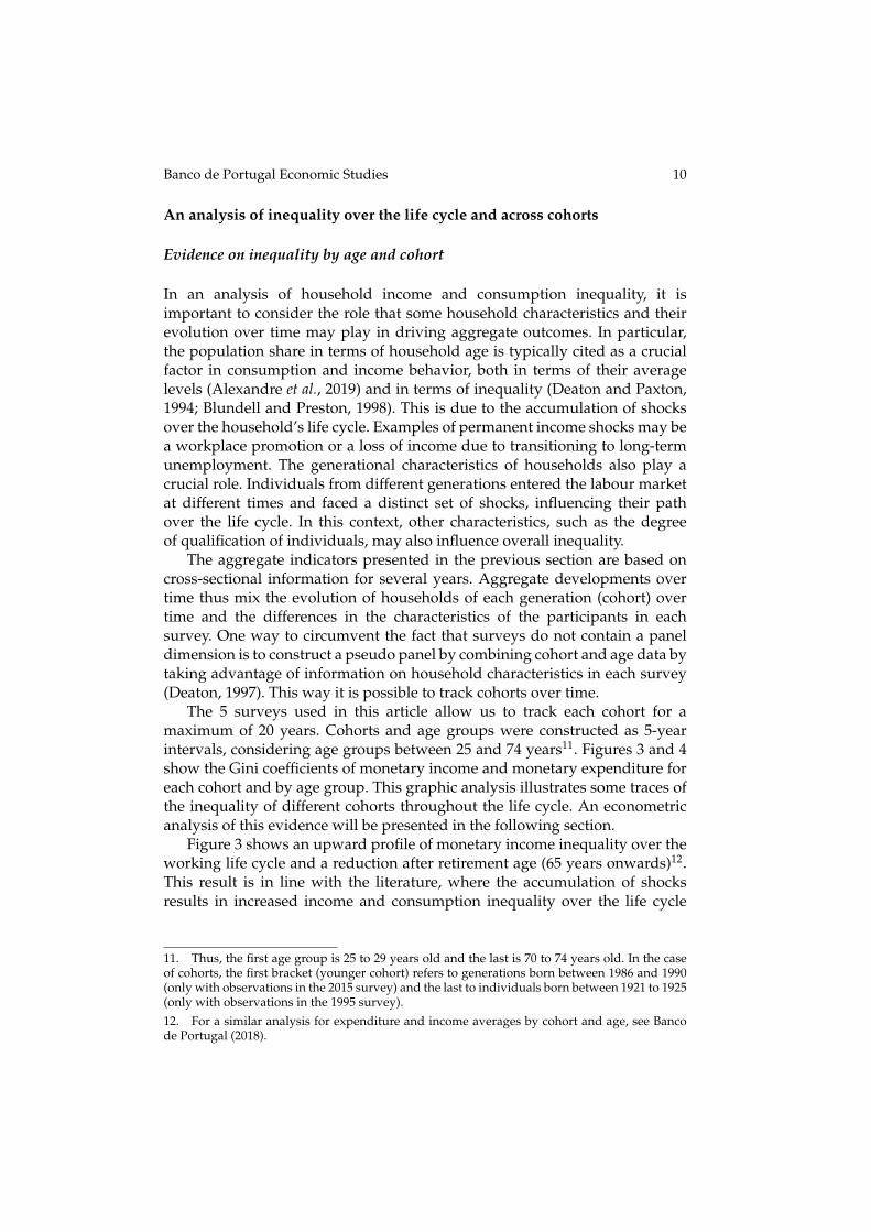
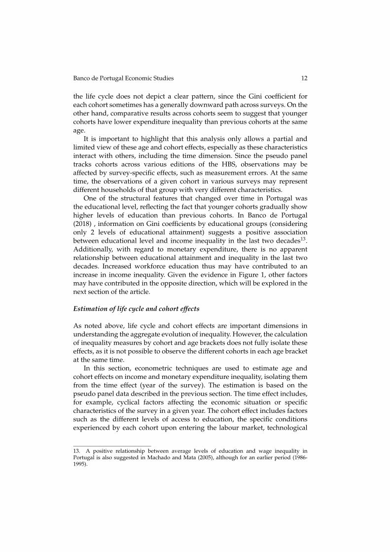
The 5 surveys used in this article allow us to track each cohort for amaximum of 20 years. Cohorts and age groups were constructed as 5-yearintervals, considering age groups between 25 and 74 years11. Figures 3 and 4show the Gini coefficients of monetary income and monetary expenditure foreach cohort and by age group. This graphic analysis illustrates some traces ofthe inequality of different cohorts throughout the life cycle. An econometricanalysis of this evidence will be presented in the following section.

Figure 3 shows an upward profile of monetary income inequality over theworking life cycle and a reduction after retirement age (65 years onwards)12.This result is in line with the literature, where the accumulation of shocksresults in increased income and consumption inequality over the life cycle

11. Thus, the first age group is 25 to 29 years old and the last is 70 to 74 years old. In the caseof cohorts, the first bracket (younger cohort) refers to generations born between 1986 and 1990(only with observations in the 2015 survey) and the last to individuals born between 1921 to 1925(only with observations in the 1995 survey).12. For a similar analysis for expenditure and income averages by cohort and age, see Bancode Portugal (2018).

11

0.20

0.25

0.30

0.35

0.40

0.45

0.50

25‐29 30‐34 35‐39 40‐44 45‐49 50‐54 55‐59 60‐64 65‐69 70‐74Age group

1986‐90 1981‐85 1976‐80 1971‐75 1966‐70 1961‐65 1956‐601951‐55 1946‐50 1941‐45 1936‐40 1931‐35 1926‐30 1921‐25

FIGURE 3: Gini coefficient of monetary income for each cohort by age group

Sources: Statistics Portugal (HBS) and authors´ calculations.Note: Age groups and cohorts were defined at 5-year intervals, as described in footnote 11.

0.20

0.25

0.30

0.35

0.40

0.45

0.50

25‐29 30‐34 35‐39 40‐44 45‐49 50‐54 55‐59 60‐64 65‐69 70‐74Age group

1986‐90 1981‐85 1976‐80 1971‐75 1966‐70 1961‐65 1956‐601951‐55 1946‐50 1941‐45 1936‐40 1931‐35 1926‐30 1921‐25

FIGURE 4: Gini coefficient of monetary expenditure for each cohort by age group

Sources: Statistics Portugal (HBS) and authors´ calculations.Note: Age groups and cohorts were defined at 5-year intervals, as described in footnote 11.

(Deaton and Paxton, 1994; Aguiar and Hurst, 2013). Regarding the values ofinequality across cohorts, the figure does not show a clear pattern of changeacross the different generations when they were the same age.

The graphical analysis of monetary expenditure inequality (Figure 4) isdifferent from that of monetary income. On the one hand, inequality through

Banco de Portugal Economic Studies 12

the life cycle does not depict a clear pattern, since the Gini coefficient foreach cohort sometimes has a generally downward path across surveys. On theother hand, comparative results across cohorts seem to suggest that youngercohorts have lower expenditure inequality than previous cohorts at the sameage.

It is important to highlight that this analysis only allows a partial andlimited view of these age and cohort effects, especially as these characteristicsinteract with others, including the time dimension. Since the pseudo paneltracks cohorts across various editions of the HBS, observations may beaffected by survey-specific effects, such as measurement errors. At the sametime, the observations of a given cohort in various surveys may representdifferent households of that group with very different characteristics.

One of the structural features that changed over time in Portugal wasthe educational level, reflecting the fact that younger cohorts gradually showhigher levels of education than previous cohorts. In Banco de Portugal(2018) , information on Gini coefficients by educational groups (consideringonly 2 levels of educational attainment) suggests a positive associationbetween educational level and income inequality in the last two decades13.Additionally, with regard to monetary expenditure, there is no apparentrelationship between educational attainment and inequality in the last twodecades. Increased workforce education thus may have contributed to anincrease in income inequality. Given the evidence in Figure 1, other factorsmay have contributed in the opposite direction, which will be explored in thenext section of the article.

Estimation of life cycle and cohort effects

As noted above, life cycle and cohort effects are important dimensions inunderstanding the aggregate evolution of inequality. However, the calculationof inequality measures by cohort and age brackets does not fully isolate theseeffects, as it is not possible to observe the different cohorts in each age bracketat the same time.

In this section, econometric techniques are used to estimate age andcohort effects on income and monetary expenditure inequality, isolating themfrom the time effect (year of the survey). The estimation is based on thepseudo panel data described in the previous section. The time effect includes,for example, cyclical factors affecting the economic situation or specificcharacteristics of the survey in a given year. The cohort effect includes factorssuch as the different levels of access to education, the specific conditionsexperienced by each cohort upon entering the labour market, technological

13. A positive relationship between average levels of education and wage inequality inPortugal is also suggested in Machado and Mata (2005), although for an earlier period (1986-1995).

13

progress or other shocks that have affected the households of a givengeneration differently from the others. Age effects include factors related tothe life cycle of households, such as the accumulation of shocks in the labourmarket and the impact of retirement on income and consumption inequality.

The main difficulty in isolating and estimating these effects results fromthe fact that the variables cohort, age and time / year of survey are perfectlycollinear (year of birth = year of survey − age). Thus, the estimation of theseeffects requires imposing restrictions. In this article, the approach proposed inHeathcore et al. (2005) was followed. The estimation uses dummies related tothe variables age, cohort and time, to estimate the effects of these 3 variablesby pseudo-panel regressions, controlling by pairs of variables. Age dummieswere used for all but one reference bracket (in this case the age group of 30-34years14). In the same way, dummies were constructed for the variables relatedto time (survey year) and cohort (year of birth). In the latter case the referencegroup corresponds to the generation born between 1921 and 1925.

The approach of Heathcore et al. (2005) proposes that effects can beestimated based on the following set of regressions:

V ar(ya,c,t) = β10 + β1

aDa + β1tDt + ε1a,c,t (1)

V ar(ya,c,t) = β20 + β2

aDa + β2cDc + ε2a,c,t (2)

V ar(ya,c,t) = β30 + β3

cDc + β3tDt + ε3a,c,t (3)

where V ar(ya,c,t) is the variance of the logarithm of the variable15 (income orexpenditure) for the group of households whose reference person belongs tothe age group a and cohort c (observed in the period t = c+ a).Da andDc, arevectors that correspond, respectively, to the sets of dummies for the age andcohort, and Dt includes the dummies for the survey year.

Thus, the effect of the life cycle (age) can be estimated alternatively usingequation 1, i.e. assuming the existence of time effects and abstracting from theeffects of cohort, or equation 2, i.e. assuming cohort effects but abstractingfrom time effects, since it is not possible to consider the 3 dimensionssimultaneously in the same equation.

Equivalently, cohort effects on inequality can be estimated by controllingfor age (equation 2) or, alternatively, controlling for the year of the survey(equation 3). It should be noted that the results are sensitive to the hypothesesadopted, as in Heathcore et al. (2005).

For the selection of regressions, we consider that it would be crucialto control for the time effect, as the sample includes a limited number of

14. For estimation purposes, the age group of 25 to 29 years was excluded, as this age grouptypically has significantly fewer observations than the others in each survey. However, resultswith and without this age group are qualitatively similar.15. The results of this analysis are robust to the use of other inequality measures, such as theGini coefficient, the coefficient of variation or percentile ratios.

Banco de Portugal Economic Studies 14

‐0.05

0.00

0.05

0.10

0.15

0.20

0.25

0.30

30‐34 35‐39 40‐44 45‐49 50‐54 55‐59 60‐64 65‐69 70‐74Chan

ges in varia

nce logarithm

 vis‐à‐vis 

the age grou

p of of 3

0‐34

 yea

rs old

Age

Monetary incomeMonetary expenditure

FIGURE 5: Life-cycle effects on income and expenditure inequality (variance oflogarithms)

Sources: Statistics Portugal (HBS) and authors´ calculations.Note: The figure represents, for each age group, the difference in the household income andmonetary expenditure variance of logarithms relative to the reference age group (30-34 years).

surveys. Thus, estimates for the life cycle effect come from the regression of thevariance of logarithm (of income or expenditure) in the age dummy and thetime dummy corresponding to the survey year (equation 1) and the estimatesfor the cohort effect come from the regression of the same variables in thecohort and time dummies (equation 3). In both regressions the estimates forthe survey year dummies coefficients are quantitatively similar. The estimatedeffects relate to the age or cohort reference groups indicated above (30-34 yearsand 1921-1925, respectively).

Based on this methodology, the set of estimated coefficients β1a represents

the life cycle effect on income and consumption inequality. These coefficientsare presented in Figure 5. The dummy coefficient for each age group measuresthe estimate of the difference in inequality (measured by the income orexpenditure variance of logarithms) for that age group relative to the 30-34years group.

The results suggest that household income and expenditure inequalityincreases over the life cycle. This result is in line with that suggested in theliterature (Blundell, 2014; Deaton and Paxton, 1994). According to life cycletheory, consumption varies over life as a function of permanent income. Theaccumulation of permanent shocks will tend to be reflected in an increase inincome inequality over the life cycle, with expenditure presenting a smootherprofile. It should be noted that estimates suggest that around retirement ageincome inequality starts declining, which is not the case for consumption.

15

‐0.3

‐0.2

‐0.1

0.0

0.1

0.2

1921

‐25

1926

‐30

1931

‐35

1936

‐40

1941

‐45

1946

‐50

1951

‐55

1956

‐60

1961

‐65

1966

‐70

1971

‐75

1976

‐80

1981

‐85

Chan

ges in logaritm of variance vis‐à‐

vis the 19

21‐192

5 coho

rt

Cohort

Monetary income

Monetary expenditure

FIGURE 6: Cohort effects on income and expenditure inequality (variance oflogarithms)

Sources: Statistics Portugal (HBS) and authors´ calculations.Note: The figure represents, for each cohort, the difference in household income and monetaryexpenditure variance of logarithms relative to the reference cohort (generation born between1921 and 1925).

Regarding the cohort evidence, Figure 6 presents the estimated coefficientsβ3c for the variance of income and expenditure of the various cohorts

compared to the cohort between 1921 and 1925.The figure shows a marked reduction in monetary income inequality for

generations born after the 1950s. In the case of monetary expenditure, areduction in inequality is estimated over all successive generations. This resultis different from that documented in the literature for the United States andthe United Kingdom (Blundell, 2014)16.

16. These life cycle and cohort effects were also estimated with an alternative methodology,inspired by Aguiar and Hurst (2013). The authors propose a normalization of the time variable(survey year) to allow the simultaneous inclusion of the three dimensions in the estimation.This transformation, originally proposed by Deaton (1997), assumes that the effects of time areorthogonal to a trend and average zero after normalization, bypassing the collinearity limitation.The methodology of Aguiar and Hurst (2013) has two steps. In a first step, the same regressionestimates the life cycle, cohort and time effects on the averages of the expenditure or incomevariable. Next, cohort and life cycle effects on inequality are estimated through a regressionfor the variance of the residuals from the previous step. The coefficients obtained with thismethodology are qualitatively similar to those presented in this article.

Banco de Portugal Economic Studies 16

The strengthening of income and consumption smoothing mechanisms

In order to understand the potential causes underlying the decrease ininequality across cohorts reported above, it is useful to refer to the analyticalframework presented in Blundell et al. (2008). These authors state that theempirical relationship between the evolution of consumption distribution andthe evolution of income distribution depends on the degree of persistenceof income shocks, on the income smoothing mechanisms and on the degreeof “insurance” (smoothing) of consumption vis-à-vis changes in income. Asregards the degree of persistence of shocks, it is well known that incomeshocks are only partially transmitted to consumption. This transmission willbe larger (smaller) the more persistent (the more transitory) the income shockis. With regard to household smoothing and risk-sharing mechanisms, theliterature emphasizes the role of wealth and savings, tax progressivity, publictransfers, intra-family transfers, informal safety nets and access to creditmarket (Heathcote et al., 2010).

Given this analytical framework, there are several possible interpretationsthat reconcile the evidence on the evolution of income and consumptioninequality in Portugal17.

One possibility is anchored in the nature of the shocks that affectedhousehold income over this period. According to this thesis, the fall inconsumption inequality could be rationalized with a lower incidence ofpermanent shocks on income over the period under review. The slight increasein income inequality in the first decade under review could also be justifiedby an increase in temporary income shocks, by nature more likely to besmoothed out in agents’ consumption decisions. Examples of these temporaryshocks are one-off increases in overtime work or a sick leave. In order totest this hypothesis, it would be necessary to have a panel database trackinghouseholds over time (Blundell et al., 2008).Thus, it is not possible to analyzethis issue with the information available in the HBS sectional data.

A second possibility is that the smoothing mechanisms available tohouseholds have increased over these two decades. It should be noted thatthis thesis can perfectly coexist with the above thesis that the persistence ofincome shocks changed over this period. Once again, it is not possible toestimate with HBS the structural evolution of the role of these mechanisms inthe Portuguese economy. Nevertheless, evidence from HBS can be combinedwith other statistical sources to characterize the impact of some of thesesmoothing mechanisms over time. The descriptive analysis below focuseson three “insurance” mechanisms that the literature identifies as central: (i)the public transfer system, (ii) the labour supply of the various household

17. One possibility would be to simply consider that measurement errors underlying eachsurvey had varied substantially and monotonically over time. This hypothesis does not seemplausible and thus will not be explored here.

17

0.34

0.36

0.38

0.40

0.42

1995 2000 2005 2010 2015

Monetary income Monetary income excluding transfers

FIGURE 7: Impact of public transfers (excluding pensions) on inequality: Ginicoefficients

Sources: Statistics Portugal (HBS) and authors´ calculations.Note: Public transfers (excluding pensions) include social transfers in support of household,housing, unemployment, sickness and disability, education and training and social inclusion.

members, and (iii) household access to the credit market. While the firsttwo mechanisms directly affect income inequality and hence consumption,the latter mechanism directly contributes to the smoothing of consumptionin the face of temporary income shocks. In order to reconcile the reductionof inequality - especially of consumption - with the functioning of thesesmoothing mechanisms, their role needs to have increased over the periodunder review.

The public transfer system to households

The public transfer system (excluding pensions) contributes to reduceinequality in all economies. In Portugal, between 1995 and 2015, the share ofcash transfers in household disposable income increased from about 3.5 percent to about 5.0 per cent. In turn, the share of transfers in kind increased fromabout 2.0 to about 2.5 per cent of household disposable income over the sameperiod.

The impact of the increase in public transfers (excluding pensions) onincome inequality can be illustrated on the basis of the HBS. Chart 7shows that the role of social transfers in decreasing income inequality hasincreased substantially over the past two decades. This result is consistentwith their increasing share of household disposable income. Chart 8 showsthat the increase in this redistributive role was concentrated on working age

Banco de Portugal Economic Studies 18

‐0.05

‐0.03

‐0.01

0.01

30‐34 35‐39 40‐44 45‐49 50‐54 55‐59 60‐64 65‐69 70‐74Age

1981‐85 1976‐80 1971‐75 1966‐70 1961‐65 1956‐60 1951‐551946‐50 1941‐45 1936‐40 1931‐35 1926‐30 1921‐25

FIGURE 8: Difference between Gini coefficients of monetary income and of monetaryincome excluding transfers, for each cohort by age group

Sources: Statistics Portugal (HBS) and authors´ calculations.Note: Negative values indicate that the monetary income Gini coefficient is lower than themonetary income Gini coefficient excluding public transfers (excluding pensions) include socialtransfers in support of household, housing, unemployment, sickness and disability, educationand training and social inclusion.

households. In addition, the effect of these transfers appears to be morepronounced in younger cohorts (compared to previous cohorts when theywere the same age).

Household labour supply

A higher participation of household members in the labour markettypically contributes to reducing income inequality and, as a consequence,consumption inequality. The fact that more than one household memberparticipates in the labour market decreases income inequality betweenhouseholds especially when individual incomes are not closely correlatedamong household members. For example, in the face of idiosyncratic labourmarket shocks that affect one individual, other family members can offsetpart of the shock through increased labour market participation (Alves andMartins, 2015). In the HBS data, the inequality of household labour income(plus pensions) is lower than the inequality of labour income (plus pensions)calculated at the individual level (Chart 9)18. This conclusion is the same for

18. These results were obtained applying the OECD equivalence scale to the households andto the respective individuals. The conclusions would be similar without the equivalization ofincomes.

19

0.00

0.10

0.20

0.30

0.40

0.50

0.60

30‐34 35‐39 40‐44 45‐49 50‐54 55‐59 60‐64 65‐69 70‐74

Gini coe

fficien

t

Age

Individuals Households

FIGURE 9: Gini coefficient of income from labour and pensions in 2015

Sources: Statistics Portugal (HBS) and authors´ calculations.Notes: For each age group the Gini coefficient of individual and household income in 2015(including zero incomes) was calculated. In the individual income calculations, each individualwas included in the age bracket corresponding to the age of his household reference person.Household income corresponds to the aggregation of individual incomes. All calculationsinclude individuals aged 25-74.

all age groups19. This suggests that the aggregation of individual incomes atthe household level contributes to reducing inequality in Portugal.

In this context, a striking fact of the Portuguese economy in recent decadesis the increasing participation of women in the labour market (Banco dePortugal, 2019). Between 1998 and 2015, the female participation rate (15-64years) in the labour market increased from about 62 per cent to about 70 percent. Together with the evidence from Chart 9, it is plausible that this higherfemale participation contributed to reducing household income inequality inPortugal. However, this is a tentative and partial equilibrium conclusion (forgeneral equilibrium analyzes, see Heathcote et al., 2017; Blundell et al., 2016).

Credit market participation

An important source of consumption smoothing against temporary incomeshocks comes from credit market participation. In fact, access to credit marketsallows smoothing out situations in which temporary income shocks makehousehold liquidity constraints binding (Blundell, 2014). These constraints are

19. Due to lack of data on individual incomes, it is not possible to replicate these computationsto the HBS surveys before 2010, which prevents an intertemporal analysis of this issue.

Banco de Portugal Economic Studies 20

particularly binding in lower-income households but may also arise in high-income households (Kaplan et al., 2014). Over the past two decades, householdparticipation in the credit market has increased substantially in Portugal for allincome brackets (Table 2)20. This increase was also observed for all age groups.This conclusion is robust whether considering access to any type of creditor just non-mortgage credit. In this period the increased participation in thecredit market may have thus contributed to reducing consumption inequalityin Portugal by allowing consumption decisions to be smoothed out in the faceof temporary income shocks.

Income percentiles % of households holding debt % of households holdingnon-mortgage debt

1994 2013 1994 2013

≤ 10 9.3 36.6 4.7 17.910-25 15.8 45.7 5.9 21.425-50 21.8 54.8 7.6 25.950-75 33.6 69.3 11.4 31.075-90 40.8 75.6 15.5 28.5> 90 35.1 78.0 14.0 25.6

Total 26.7 60.7 9.8 26.1

TABLE 2. Credit market participation

Sources: Households’ Wealth and Indebtedness Survey (1994) and Portuguese HouseholdFinance and Consumption Survey (2013).Note: Calculations for households whose reference person is younger than 65 years old.

Conclusions

This paper sought to characterize the evolution of household income andexpenditure inequality in Portugal in the period 1995-2015. Based on apseudo panel, the role of the life cycle in household inequality and theevolution of this inequality across cohorts was estimated. A striking featurein the Portuguese economy is the decrease in consumption inequality insuccessive cohorts. The article suggests that the strengthening of income andconsumption smoothing mechanisms in the Portuguese economy may havecontributed to this evolution.

20. The authors thank Sónia Costa and Luísa Farinha for the computations underlying Table 2.

21

This article opens avenues to several studies on the estimation andstudy of the factors underlying the evolution of income and consumptioninequality in Portugal. These structural factors also provide insights onfuture developments of inequality. These include the ageing population,the increasing participation of women in the labour market, improvededucational attainment of individuals and the potential reinforcement ofinsurance networks available to households. The joint modeling of theseelements is a demanding challenge for future research.

Banco de Portugal Economic Studies 22

References

Aguiar, M. and C. Hurst (2013). “Deconstructing Life Cycle Expenditure.”Journal of Political Economy, 121(3), 437–492.

Alexandre, F., P. Bação, and M. Portela (2019). “Is the basic life-cycle theory ofconsumption becoming more relevant: Evidence from Portugal.” Review ofthe Economics of the Household.

Alves, N. and C. Martins (2015). “Income smoothing mechanisms after labormarket transitions.” Working papers 201510, Banco de Portugal.

Banco de Portugal (2018). “Household consumption inequality in Portugal.”Special Issue, Economic Bulletin, Banco de Portugal, June.

Banco de Portugal (2019). “Demographic changes and labour supply inPortugal.” Special Issue, Economic Bulletin, Banco de Portugal, June.

Blundell, R. (2014). “Income Dynamics and Life-Cycle Inequality: Mechanismsand Controversies.” The Economic Journal, 124, 289–318.

Blundell, R., M. Costa Dias, C. Meghir, and J. Shaw (2016). “Female laborsupply, human capital and welfare reform.” Econometrica, 84(5), 1705–1753.

Blundell, R., L. Pistaferri, and I. Preston (2008). “Consumption Inequality andPartial Insurance.” American Economic Review, 95(5), 1887–1921.

Blundell, R. and I. Preston (1998). “Consumption inequality and incomeuncertainty.” Quarterly Journal of Economics, 11(3), 603–640.

Cantante, F. (2019). O risco da desigualdade. Edições Almedina, Coimbra.Costa, S., L. Farinha, L. Martins, and R. Mesquita (2020). “Portuguese

Household Finance and Consumption Survey: results for 2017 andcomparison with the previous waves.” Banco de Portugal, Economic studies,6(1).

Deaton, A. and C. Paxton (1994). “Intertemporal choice and inequality.”Journal of Political Economy, 102(3), 437–467.

Deaton, Angus (1997). The analysis of household surveys: a microeconometricapproach to development policy. The World Bank.

Gouveia, Miguel and José Tavares (1995). “The distribution of householdincome and expenditure in Portugal: 1980 and 1990.” Review of Income andWealth, 41(1), 1–17.

Heathcore, J., K. Storesletten, and G. Violante (2005). “Two Views of Inequalityover the Life Cycle.” Journal of the European Economic Association, 3(2-3), 765–775.

Heathcote, Jonathan, Fabrizio Perri, and Giovanni L Violante (2010). “Unequalwe stand: An empirical analysis of economic inequality in the United States,1967-2006.” Review of Economic dynamics, 13(1), 15–51.

Heathcote, Jonathan, Kjetil Storesletten, and Giovanni L Violante (2014).“Consumption and labor supply with partial insurance: An analyticalframework.” American Economic Review, 104(7), 2075–2126.

Heathcote, Jonathan, Kjetil Storesletten, and Giovanni L Violante (2017). “Themacroeconomics of the quiet revolution: Understanding the implications

23

of the rise in women’s participation for economic growth and inequality.”Research in Economics, 71(3), 521–539.

Jenkins, Stephen (2015). “Svylorenz: stata module to derive distribution-freevariance estimates from complex survey data, of quantile group shares of atotal, cumulative quantile group shares.”

Kaplan, Greg and Giovanni L. Violante (2018). “Microeconomic heterogeneityand macroeconomic shocks.” Journal of Economic Perspectives, 32(3), 167–94.

Kaplan, Greg, Giovanni L. Violante, and Justin Weidner (2014). “The WealthyHand-to-Mouth.” Brookings Papers on Economic Activity, 45(1 (Spring), 77–153.

Krueger, Dirk, Fabrizio Perri, Luigi Pistaferri, and Giovanni L. Violante (2010).“Cross-sectional facts for macroeconomists.” Review of Economic dynamics,13(1), 1–14.

Machado, José and José Mata (2005). “Counterfactual decomposition ofchanges in wage distributions using quantile regression.” Journal of appliedEconometrics, 20(4), 445–465.

Rodrigues, C., F. Figueiras, and V. Junqueira (2016). “Inequality of income andpoverty in Portugal.” Research studies, Fundação Francisco Manuel dosSantos.

Statistics Portugal (1997). Household Budget Survey 1995.Statistics Portugal (2002). Household Budget Survey 2000.Statistics Portugal (2008). Household Budget Survey 2005/2006.Statistics Portugal (2012). Household Budget Survey 2010/2011.Statistics Portugal (2017). Household Budget Survey 2014/2016.