A CGE Analysis of Border Adjustments Under the Cap-and-Trade System: A Case Study of the Japanese Economy

Electronic copy available at: http://ssrn.com/abstract=1907108

1

A CGE Analysis of Border Adjustments under the Cap-and-Trade System: A

Case Study of the Japanese Economy

Shiro Takeda

Tetsuya Horie†

Toshi H. Arimura‡

July, 2011

Abstract

Using a multi-region and multi-sector CGE model, this paper evaluates the impact of border

adjustment policies of carbon regulations on the Japanese economy. We consider the following six

scenarios: 1) no border adjustment, 2) carbon tariffs on imports based on the carbon content in

foreign exporters’ production, 3) carbon tariffs on imports based on the carbon content in domestic

production (BID), 4) carbon tariffs on imports and rebates on exports based on the carbon content in

domestic production (BIED), 5) BID applied only to the EITE (energy-intensive trade-exposed)

sectors, and 6) BIED applied only to the EITE sectors. In particular, we examine the impact of the

border adjustment policies on the welfare of the Japanese economy, carbon leakage, and the

competitiveness of the Japanese EITE sectors.

Our analysis shows that no single border adjustment policy is superior to the other policies in

terms of simultaneously solving all three issues: welfare impacts, carbon leakage, and the loss of

competitiveness in the EITE sectors. In addition, we show that export border adjustment often plays

a crucial role in Japan. This insight is interesting because the policy debate on border adjustment is

often biased toward import border adjustment. Our analysis also reveals that border adjustment in

Japan significantly affects carbon leakage to China and the competitiveness of the iron and steel

sector. Finally, we show that border adjustments with and without consideration to indirect emissions

have similar impacts, which indicates that the information regarding direct emissions is enough to

implement border adjustment in Japan.

Keywords: CGE analysis; Climate change; border adjustment; carbon leakage, competitiveness

JEL Classification: C68, F18, Q54, Q56

Kanto Gakuen University and Sophia University Center for the Envirionment and Trade Research. Email:

[email protected] † Sophia University Center for the Environment and Trade Research, Sophia University ‡ Sophia University and Center for the Environment and Trade Research.

Electronic copy available at: http://ssrn.com/abstract=1907108

2

1. Introduction

Developed nations are considering the adoption of carbon-pricing policies, such as domestic

emissions-trading schemes or carbon taxes to counter climate change. At the same time, developing

countries that are Non-Annex I Countries under the Kyoto Protocol are putting off the introduction

of emissions restrictions. It is projected that such internationally asymmetrical adoption of emissions

restrictions could bring about a situation in which developed countries restrain CO2 emissions, while

developing countries undergo increased production and emissions in carbon-intensive industries.

This problem, in which adoption of policies to restrain carbon emissions in one region results in an

increase in CO2 emissions in regions that have not adopted such policies, is referred to as carbon

leakage. At the same time, it has been mentioned that the international competitiveness of

carbon-intensive industries in developed countries could decrease in comparison with that of

industries in developing countries that do not need to bear the costs associated with restraining

emissions. Recently, a lively debate have occurred on the introduction and efficacy of border

adjustments (BAs) as a solution to these issues of carbon leakage and reduced international

competitiveness. Border adjustments in this context refer to trade policies intended to compensate

for disadvantages resulting from CO2 emission regulations. In this study, we will perform

quantitative verification of the effects of border adjustments on restraining carbon leakage and

decreases in the international competitiveness of the domestic industry in Japan. In addition, we will

examine the effects of border adjustments on welfare levels in the event of the introduction of

carbon-pricing policies, such as a carbon tax or an emissions-trading scheme in Japan.

Measures have been proposed in recent years to counter carbon leakage and decreases in

international competitiveness resulting from the adoption of emissions-trading schemes, such as the

Waxman-Markey bill, the Kerry-Boxer bill, and the Cantwell-Collins bill in the United States.

Border adjustments have garnered particular attention. In particular, the Waxman-Markey bill, which

3

passed the U.S. House of Representatives in 2009, proposed refunding the majority of the costs of

emissions caps if an energy-intensive trade-exposed (EITE) industry is determined to address the

problem of carbon leakage. It also proposed granting the president the authority to implement border

adjustments requiring the purchase of carbon credits for products imported from countries with no

emissions restrictions. This truly resembles border adjustments that would assess a carbon tax as a

tariff. A similar debate is underway in Europe as well. In Europe, a CO2 emissions-trading scheme

known as EU-ETS took effect beginning in 2005. With the shift from Phase I to the following phase,

the percentage of carbon credits distributed free of charge decreased slightly (from 95% in Phase Ito

90% in Phase II). In Phase III, beginning in 2012, the distribution of free credits will decrease and

the system will shift to an auctioning scheme. In doing so, in consideration of the impact on the

European industry, the European Commission has already decided to establish cost-mitigating

measures (European Commission 2010). In this debate, President Sarkozy of France argued for the

need to enable appropriate border adjustments against countries whose efforts are inadequate, and

the leaders of each European nation are strongly interested in border adjustments as well.1

In Japan, during the debate on the introduction of carbon-pricing policies,2 the issues of carbon

leakage and decreasing international competiveness, resulting from an increase in production costs

faced by the domestic industry, have emerged as the greatest topics of concern. While border

adjustments have enjoyed considerable attention as countermeasures against these issues in policy

debate, no studies have verified quantitatively the degree of impact of enacting border adjustments in

the event of the adoption of carbon-pricing policies in Japan. Furthermore, the term "border

adjustment" actually encompasses a variety of types of adjustments. The first of these is an import

1 Multilateral Trade System Department, Trade Policy Bureau, Ministry of Economy, Trade and Industry of Japan.

2010 Report on Compliance by Major Trading Partners with Trade Agreements—WTO, FTA/EPAs, BITs.

http://www.meti.go.jp/report/downloadfiles/g100402a03j.pdf 2 Meeting beginning in April 2010, the Global Environment Subcommittee of the Central Environmental Council is

deliberating on the design of an emissions-trading scheme in Japan. Furthermore, in the Ministry of Finance’s Study

Group on the Environment and Tariff Policies, which met from March through June 2010, discussions proceeded with

a focus on solutions to the problem of carbon leakage and decreased international competitiveness of the domestic

industry accompanying the adoption of an emissions-trading scheme.

4

tariff applied based on the volume of carbon emitted in the production of imported goods to ensure

fairness in domestic markets. This import tariff has two types: an import tariff based on the

emissions coefficient in the importing country (Japan) and an import tariff based on the emissions

coefficient in the exporting (foreign) country. The next type of a border adjustment is a measure

providing rebates of the cost of carbon prices for goods exported from Japan (export subsidies) to

maintain fairness in overseas markets. In this case, it is conceivable that border adjustments could be

enacted in such a way as to utilize both import tariffs and export subsidies simultaneously.

Furthermore, some measures could apply these import tariffs and export subsidies to the industry as

a whole, while others could be implemented by limiting their application to certain industries.

Analysis of the efficacy of border adjustments, which in this way cover a diverse range of measures

for restricting carbon leakage and decreases in international competitiveness, can provide valuable

information for the formulation of carbon-pricing policies in Japan.

Recently, studies on the subject of border adjustments have been conducted. Fischer and Fox

(2009) and Böhringer et al. (2010) compared various measures (border adjustments and gratis

allocation of emissions permits) to tackle the leakage and competitiveness issues. However, they

only investigated policies in the U.S., Canada and EU. Alexeeva et al. (2008) conducted a

comparative analysis of the two counter measures against leakage and decreases in the

competitiveness of border adjustments and integrated emissions trading, employing theoretical and

demonstrative methods (CGE analysis). While their study introduced a new point of comparison

with the policy of integrated emissions trading, it addressed only simple border adjustment rules.

Furthermore, the subject of its simulation analysis was the European EU-ETS emissions restrictions.

Using a CGE model, Winchester (2011) analyzed border adjustments with alternative firm behaviors.

Kuik and Hofkes (2009) again used CGE analysis to analyze the effects of border adjustments.

While their study is outstanding in analyzing the effects in each sector in detail, like Alexeeva et al.

(2008), the subject of the analysis is EU emissions restrictions only. Mattoo et al. (2009) used CGE

5

analysis to analyze emissions restrictions accompanying border adjustments in developed countries.

While their study also took into consideration Japan’s border adjustments, not just those of Europe

and North America, and analyzed a diverse range of border adjustment policies, the main subjects of

the analysis were North America, Europe, and developing countries, without looking at the impact

on Japan in depth. Thus, as outlined above, the subjects of the existing studies have, for the most part,

been Europe and North America, with no study having conducted a detailed analysis of Japan.

Therefore, the contribution of this paper is to compare a diverse range of measures to prevent

leakage and maintain competitiveness by analyzing the detailed impacts on Japan of that nation’s

border adjustment policies, with Japan as the main subject of the analysis.

In this study, we employ simulation analysis using a multi-region, multi-sector computable

general equilibrium model (CGE model). The model is a 14-region, 26-sector static CGE model,

developed by improving on the GTAP-EG model, using as benchmark data the GTAP 7 database

with 2004 as the base year. Assuming that Japan adopts a policy of reducing emissions by 25% from

1990 levels in the form of a cap-and-trade emissions-trading scheme, we analyze the kind of impact

that the adoption of border adjustments would have in such a case. Specifically, we address the

following six policy scenarios: (1) no border adjustment, (2) border adjustments on imports based on

emissions coefficients in the exporting (foreign) country, (3) border adjustments on imports based on

emissions coefficients in Japan (the importing country), (4) border adjustments on both imports and

exports, (5) border adjustments on imports in energy-intensive trade-exposed (EITE) industries only,

and (6) border adjustments on exports and imports in EITE industries only. We compare these from

the standpoints of welfare effects, carbon leakage, and international competitiveness in EITE

industries.

The major results of our analysis are as follows. Our analysis shows that no single border

adjustment policy is superior to the other policies in terms of simultaneously solving all three issues:

retaining welfare levels, mitigating carbon leakage, and suppressing the loss of competitiveness in

6

the EITE sectors. This finding means that the type of border adjustment to be adopted depends on

the issue of priority. In addition, we show that export border adjustment often plays a crucial role in

Japan. This insight is interesting because the policy debate on border adjustment is often biased

toward import border adjustment. Our analysis also reveals that border adjustment in Japan

significantly affects carbon leakage to China and the competitiveness of the iron and steel sector.

This finding indicates that we need to give special consideration to China and the iron steel sector in

designing a border adjustment policy in Japan. Finally, border adjustments with and without

consideration to indirect emissions have similar impacts, indicating that the information on direct

emissions is enough to implement border adjustment in Japan.

The rest of the paper is organized as follows. Section 2 describes the CGE model and data used

in our analysis, while section 3 defines the emissions-trading scheme and border adjustments

analyzed. In section 4, we discuss the results of the analysis from the perspective of welfare levels,

carbon leakage and international competitiveness under an emissions-trading scheme. Next, in

section 5, we conduct a sensitivity analysis, and we compare the advantages and disadvantages

among different border adjustment policies in section 6. Finally, we present our conclusions in

section 7.

2. Model and Data

2.1. Model

We construct a static CGE model with 14 regions and 26 sectors, as listed in Table 1. The structure

of the model is similar to GTAP-EG (Rutherford and Paltsev 2000, Paltsev 2001, Fischer and Fox

2007, Takeda et al. 2011). The details of the model structure are provided in the Appendix. We

assume perfect competition in all markets and that production is subject to constant returns to scale

7

technology (CES production functions). The production sectors are divided into two types, fossil

fuel and non-fossil fuel sectors, and we assume that these have different production structures.

Fossil fuel production activities include the extraction of coal (COA), crude oil (OIL), and gas

(GAS). Production has the structure shown in Figure 1. Fossil fuel production is basically the same

as in the GTAP-EG model. Fossil fuel output is produced as a constant elasticity of substitution

(CES) aggregate of natural resources and non-natural resources input composite. The non-natural

resources input is a Leontief composite of capital, labor and other intermediate inputs.

Non-fossil fuel production (including electricity) has the structure in Figure 2. Non-fossil fuel

production is also basically the same as in the GTAP-EG model. Output is produced with Leontief

aggregation of non-energy goods and an energy-primary factor composite. The energy-primary

factor composite is a nested CES function of energy goods and primary factors. With respect to the

petroleum and coal products sector, we assume that crude oil enters into the production function at

the top-level Leontief nest because most of crude oil is used as feedstock. Similarly, for the chemical

products sector, we divide its energy use into feedstock requirements, which are treated as

non-energy intermediate inputs, and the remainder. For this, we use the feedstock ratio data of Lee

(2008).

The demand side of each economy is represented by the representative household. The

representative household's utility has the structure depicted in Figure 3. The representative agent

makes decisions to maximize utility subject to the budget constraint. The household's income

consists of factor income minus tax payment. We assume that the endowments of primary factors are

exogenously constant. International trade in goods is treated in the same way as the GTAP model

(Hertel, 1997), and there is no international movement of primary factors. In addition, we assume

that government expenditure and investment are held constant at the benchmark values.

2.2. Benchmark Data and Parameters

8

For the benchmark data, we employ the GTAP 7 database with 2004 as the base year. For CO2

emissions data, we use the data provided by Lee (2008), but CO2 emissions of the Japanese iron and

steel sector (I_S) in her data are lower than the actual value. Because I_S is of great importance in

the analysis of emissions regulation, we correct the data according to the data provided by 3EID

(Nansai and Moriguchi, 2010). For elasticity parameters in production functions, we use the values

of Fischer and Fox (2007) and GTAP data, and for Armington elasticity parameters, we use GTAP

values. Elasticity of substitution between resource and non-resource inputs in the fossil fuel sectors

(e_es(j) in Figure 1) is calibrated from the benchmark supply elasticity of fossil fuels, which is

assumed to be two for all fossil fuels.

To grasp the characteristics of Japanese economy, let us see the data of Japanese economy.

Figure 4 depicts the carbon intensity (tons of CO2 per 1,000$ output) of each sector in Japan. As

expected, iron-steel (I_S), non-metallic minerals (NMM), non-ferrous metal (NFM), chemical

products (CRP), paper-pulp products (PPP), and transport sectors (OTP, ATP, WTP) have high

carbon intensity. In addition, the fishery (FSH) sector also has a large intensity in Japan. These

sectors are likely to be significantly affected by carbon regulations. According to carbon intensity,

we categorize I_S, FSH, NMM, OMN, CRP, NFM and PPP as energy-intensive trade-exposed

(EITE) sectors. Figure 5 reports the export and import shares of Japan by destination and source. It

shows that China (CHN), Korea (KOR), and other Asian regions (ASI), which are not obliged to

reduce CO2 emissions, are Japan’s large trade partners. This finding suggests that emissions

regulation in Japan is likely to damage the competitiveness of EITE sectors in Japan compared to

those in China, Korea, and other Asian countries.

3. Permit Trading System and Border Adjustment

9

3.1. Permit Trading System

We assume that the Japanese government will introduce a cap-and-trade permit trading system.

Moreover, we assume that permits are allocated to sectors through an auction. The targeted CO2

reduction is set at a 30% reduction from the 2004 levels of CO2 emissions, which is almost

equivalent to a 25% reduction from the 1990 levels. It is well known that a cap-and-trade permit

trading system with an auction scheme has the same impact on an economy as emission tax. Thus,

we can interpret this policy as a carbon tax as well. We also assume that the revenue from the

auction is returned to the representative household in a lump-sum fashion.

Note that we assume that only Japan implements a cap-and-trade system and no other regions

regulate carbon emissions. It is because our main aim is to analyze the Japanese economy and

because the assumption of unilateral policy by Japan will clarify the pure impacts of Japanese border

adjustments. However, in the sensitivity analysis, we consider the case where the US and the EU as

well as Japan impose carbon regulations.

3.2. Border Adjustment Policies

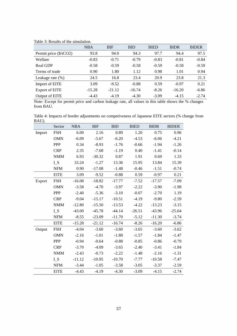
We consider six policy scenarios to mitigate carbon leakage and the loss of competitiveness. Table 3

summarizes the characteristics of the scenarios. NBA is the no border adjustment scenario. BIF

involves a carbon tariff on imports based on the carbon content in foreign production. BIF is the

carbon content tariff in the true sense of the term. However, BIF has some difficulties in

implementation because it requires a lot of information on energy use in foreign countries. Thus, we

consider another type of carbon tariff, BID, which involves assigning a carbon tariff to all imported

products based on the carbon content in Japanese domestic production.

In BIED, border adjustment is applied to both imports and exports (BID + export border

10

adjustment). In this scenario, the carbon tariff on imports is based on carbon content in domestic

production, and the additional costs of domestic production incurred by this carbon pricing policy

are rebated when the products are exported from Japan. Comparison between BID and BIDR will

show the additional impacts generated by export border adjustment. Scenario BIDR limits the

sectors to which the BID is applied to the EITE sector. In BIEDR, the sectors to which the BIED is

applied are also limited to the EITE sector.

The carbon tariff and export rebate are determined according to the carbon content based on

direct and indirect emissions.3 Denote 𝑞𝑖𝑟

𝐶𝑂2𝑇 to be the total amount of CO2 emitted from a given 𝑖

th sector in a given region 𝑟. 𝑞𝑖𝑟𝐶𝑂2𝑇 is defined as the sum of the direct and indirect emissions:

𝑞𝑖𝑟𝐶𝑂2𝑇 = 𝑞𝑖𝑟

𝐶𝑂2𝐷 + 𝑞𝑖𝑟𝐶𝑂2𝐼𝐷

where 𝑞𝑖𝑟𝐶𝑂2𝐷 and 𝑞𝑖𝑟

𝐶𝑂2𝐼𝐷 are the direct and indirect CO2 emissions at the 𝑖th sector in region 𝑟,

respectively. The direct emission of CO2 is defined as the amount of CO2 emitted from fossil fuel use.

Thus, the direct emission is given as:

𝑞𝑖𝑟𝐶𝑂2𝐷 = ∑𝜙𝑒𝑖𝑟𝑞𝑒𝑖𝑟

𝑒

where 𝜙𝑒𝑖𝑟 is the emissions coefficient of fossil fuel 𝑒 in sector 𝑖 of region 𝑟 and 𝑞𝑒𝑖𝑟 is the

amount of fossil fuel used in sector 𝑖 of region 𝑟. The indirect emissions are the amount of CO2

embodied in the purchased electricity (CO2 emitted at power plants where electricity is generated by

burning fossil fuels). We calculate the indirect emission from sector 𝑖 in the following manner. First,

define 𝜃𝑖𝑟𝐸𝐿𝑌 as the share of electricity used in sector 𝑖 (𝑑𝑖𝑟

𝐸𝐿𝑌) over the total quantity of electricity

supplied in region 𝑟 (𝑞𝐸𝐿𝑌,𝑟):

𝜃𝑖𝑟𝐸𝐿𝑌 = 𝑑𝑖𝑟

𝐸𝐿𝑌 𝑞𝐸𝐿𝑌,𝑟⁄

Letting 𝑞𝐸𝐿𝑌,𝑟𝐶𝑂2𝐷 be the direct emission of CO2 from the electricity sector, we can calculate the

indirect emission of CO2 from sector 𝑖 by multiplying 𝑞𝐸𝐿𝑌,𝑟𝐶𝑂2𝐷 by 𝜃𝑖𝑟

𝐸𝐿𝑌:

3 Indirect emissions in this paper mean emissions embodied in electricity. We do not consider emissions embodied in

intermediate inputs because it is difficult (or maybe impossible) to calculate them in a CGE model, which assumes

substitution among inputs.

11

𝑞𝑖𝑟𝐶𝑂2𝐼𝐷 = 𝜃𝑖𝑟

𝐸𝐿𝑌𝑞𝐸𝐿𝑌,𝑟𝐶𝑂2𝐷.

Then, the carbon content of a unit of product of sector (𝜉𝑖𝑟), which is the quantity of CO2

emissions contained in a unit of production, is given as:

𝜉𝑖𝑟 = 𝑞𝑖𝑟𝐶𝑂2𝑇 𝑞𝑖𝑟⁄

In the carbon tariff based on the domestic emissions coefficient, the tariff rate assigned to a unit of

imported product of sector 𝑖 of region 𝑟 is defined by:

𝜏𝑖𝑟 = 𝑝𝑟𝐶𝑂2𝜉𝑖𝑟

where 𝑝𝑟𝐶𝑂2is the price of a permit in the region 𝑟. On the other hand, in the carbon tariff based on

the foreign emissions coefficient, the tariff rate assigned to a unit of imported product of sector 𝑖

from region 𝑠 to 𝑟 is defined by:

𝜏𝑖𝑠𝑟 = 𝑝𝑟𝐶𝑂2𝜉𝑖𝑠

In export rebates, a subsidy of 𝜏𝑖𝑟 is applied to export goods 𝑖 from region 𝑟.

In the sensitivity analysis, we consider the case where emissions coefficient is based only

on the direct emissions. In this case, 𝜉𝑖𝑟 is calculated as follows:

𝜉𝑖𝑟 = 𝑞𝑖𝑟𝐶𝑂2𝐷 𝑞𝑖𝑟⁄

4. Results

We first compare the effects of six separate policies on welfare, carbon leakage and the

competitiveness of the Japanese EITE. We measure carbon leakage with the conventional metric of

the carbon leakage rate, which is defined by the fraction of the increase in foreign emissions over the

decrease in domestic emissions induced by the carbon pricing policy. We also measure the change in

competitiveness of the Japanese EITE sectors by the percent change in their production. Welfare is

defined as the utility levels of the representative household in Japan. The results are summarized in

Table 3.

12

4.1. Welfare Impacts

Let us first examine welfare impacts. Border adjustments with only carbon tariffs, such as BIF, BID,

and BIDR, yield better welfare levels than NBA. This finding is mainly due to the effect of

improvement on the terms of trade. BIF, BID, and BIDR are policies in which import tariffs are

increased by the imposition of a carbon tariff. Such increases in import tariffs decrease the world

price of imports, thereby improving the terms of trade in Japan, and thus the welfare of the Japanese

economy is also improved. Table 3 shows the percent changes in the terms of trade in Japan for each

scenario. In the scenario of NBA, the terms of trade are increased 0.9% from BAU. However, the

terms of trade increase more significantly in the scenario of a border adjustment that imposes only a

carbon tariff. In particular, in BIF, the terms of trade increase by 1.8% from BAU.

On the other hand, results in BIDE and BIDER show that the combined policies of import and

export border adjustments have similar welfare impacts to NBA. The reason why welfare in BIDE

and BIDER is inferior to BID and BIDR is the higher permit price and the smaller improvement of

the terms of trade. Export border adjustment restores the competitiveness of Japanese firms and

stimulates the production of EITE sectors. This requires the higher emissions permit price (marginal

abatement cost) to satisfy the emission limit and lowers the welfare level. In addition, export border

adjustments have an effect similar to export subsidies and lower the world price of exported goods.

This deteriorates Japan’s terms of trade and lowers the welfare level.

Border adjustment policies were originally designed to sustain the competitiveness of domestic

industries and to suppress carbon leakage; they were not designed to improve welfare levels.

However, as the above results show, border adjustment policies that impose only a carbon tariff on

imports can improve the welfare impacts of carbon regulation.

13

4.2. Carbon Leakage

Next, we compare leakage rates among the policy scenarios. The fifth line in Table 3 shows the

leakage rates (%). As expected, the highest leakage rate (24.45%) is observed when no border

adjustment policy is conducted (i.e., NBA). Among all of the policy scenarios, the policy scenario in

which a carbon tariff based on a foreign emission coefficient is adopted (i.e., BIF) is the most

effective policy to suppress the carbon leakage. In BIF, the leakage rate decreases to 16.78% from

24.45% in NBA. The emission coefficient in foreign countries is generally higher than in Japan, and

thus a carbon tariff based on a foreign coefficient has higher rates. This makes the effect of the

carbon tariff based on a foreign emissions coefficient strong. In addition, carbon tariffs in BIF are

differentiated across regions and thus work more effectively in restraining carbon leakage.

BID and BIDR show that border adjustments on imports based on domestic emissions

coefficients also reduce carbon leakage, but the decrease in the leakage rate is very small. On the

other hand, with BIDE and BIDER in which an export border adjustment is added to BID and BIDR,

the leakage rate reduces by 3 points compared to NBA. This finding indicates that export border

adjustment plays a more important role in restraining carbon leakage. Finally, a comparison of BID

and BIDR shows that limiting border adjustment sectors to EITE increases carbon leakage, although

only slightly. This finding means that limiting border adjustment sectors to EITE is undesirable for

restraining carbon leakage. A similar argument is applied to BIDE and BIDER. Because carbon

leakage occurs through an energy channel as well as a trade channel, the leakage cannot be

thoroughly suppressed by border adjustment policies.4 However, our analysis shows that border

adjustment has a certain effect in restraining carbon leakage.

Figure 4 shows the changes in the CO2 emission in foreign countries induced by the

4 Carbon leakage through the energy channel occurs through the energy market. The demand for energy decreases in

the country in which a carbon pricing policy is introduced. This decreases the price of energy in the international

energy market, thereby increasing the demand for energy increases in foreign countries in which the carbon pricing

policy is not introduced. This leakage occurs regardless of sector competitiveness.

14

introduction of carbon pricing policy and BAs.5 First, by observing NBA, we find that the

introduction of a carbon pricing policy in Japan increases CO2 emissions in all the regions. However,

there is a substantial difference in emission changes among countries. In IND, KOR, OOE, and

ROW, the increase of CO2 emissions is very small; the highest increase among these countries is 5

MtCO2. Furthermore, the introduction of BAs in Japan increases emissions in these countries by no

more than 1 MtCO2, which is considered a limited impact. Conversely, in countries such as CHN,

ASI, USA, EUR, and MPC, CO2 emissions increase significantly with the introduction of a

Japanese carbon pricing policy. These countries also show significant variations in the impact of

border adjustments. In particular, CHN experiences the largest increases in CO2 among these

countries (23.5MtCO2). This increase is twice as large as the second highest emission increase,

which occurs in ASI.

It is also worth mentioning that when different border adjustments are adopted, CO2 emissions

fluctuate substantially more in China than in any other region. This finding implies that border

adjustments in Japan affect China much more significantly than any other region. Because China

accounts for the largest carbon leakage in the world induced by the Japanese carbon pricing policy,

the impact of border adjustments on worldwide carbon leakage depends on their impact on CO2

emissions in China. This result implies that China is a key country to consider when introducing

carbon pricing policy and its corresponding border adjustments.

4.3. Competitiveness of EITE Sectors

Finally, we examine the impact of border adjustments on Japanese EITE sector competitiveness. The

sixth to eighth lines in Table 3 report percentage changes in the import, export and output of EITE

sectors. The table shows that NBA increases the amount of imports of EITE goods by 3.09% from

5We omit BRA, OEU, and CAN from Figure 6 because the changes in CO2 emissions in these countries are almost

zero.

15

BAU. This is because the costs of domestic production and therefore the price of the domestic

products of the EITE sectors increase, and their competitiveness is lost in the domestic market. The

introduction of border adjustments eases this increase in imports; the increase in imports is decreased

from 3.09% in NBA to 0.59% and 0.21% in BIED and BIEDR, respectively.

On the other hand, in BIF, BID, and BIDR, the amount of imports decreases from the BAU

level. An extreme case of this is BIF, in which the amount of imports decreases 9.52% from the BAU

case. This finding suggests that imported products are less competitive in the Japanese domestic

market when the border adjustments are applied than in the BAU case, which can be considered

overprotection of Japanese domestic products in the domestic market.

The introduction of the carbon pricing policy also decreases the competitiveness of Japanese

domestic products exported to foreign regions. The impact of the carbon pricing policy on exports is

much greater than the impact on imports. For example, in NBA, exports from the EITE sector

decrease by 15.28% from the BAU case. We now must question to what extent border adjustment

policies can improve this number. If carbon tariffs were only imposed on imported products (BIF,

BID, and BIDR), the exports from the EITE sector would be smaller than in NBA. This means that

the competitiveness of exported goods deteriorates as a result of border adjustment only for imported

goods.

On the other hand, if rebates are given to exported Japanese products (BIED and BIEDR), the

decrease in exports eases significantly, from a 15.28% decrease in NBA to a 8.26% and 6.86%

decrease in BEIDE and BIEDR, respectively. Therefore, to mitigate the negative impact of carbon

pricing policy on exports, rebates on exports must be included in border adjustment policies because

a border adjustment policy with only carbon tariffs will not improve the negative effects.

With NBA, output decreases due to the increase in imports and decrease in exports. As we

mentioned earlier, a border adjustment policy with only carbon tariffs (BIF, BID, BIDR) causes

exports to decrease even more. Thus, such border adjustment policies improve the output level from

16

the NBA case only slightly. On the other hand, the combined border adjustments (BIED and BIEDR),

which significantly alleviate the decrease in exports, improve the output of EITE sectors. This

finding suggests that to retain the output levels, it is important to include both carbon tariffs and

export rebates in the border adjustment policy.

Regarding individual EITE sectors, we find that the results for most of the EITE sectors are the

same as the aggregate results for all EITE sectors (Table 4). The I_S (iron and steel sector) is worth

examining separately because it receives the greatest effects of the carbon pricing and border

adjustment policies among all of the sectors. In the NBA case, the amount of imports increases by

33%, the amount of exports decreases by 43%, and output decreases by 15%. Because the impacts of

the introduction of the carbon pricing policy are very large, the impacts of the border adjustment

policies are significant as well. In BIED, the increase in imports is reduced by half, and the decreases

in exports and outputs are reduced to half and two-thirds of previous values, respectively. These

results suggest that border adjustment policy can have a crucial role in determining the impacts on

individual sectors.

5. Sensitivity Analysis

In this section, we conduct sensitivity analyses by changing assumptions in the benchmark analysis.

First, we change the assumption emissions coefficients used to calculate the carbon tariff and export

rebate. In the analysis of the previous sections, we include not only direct emissions (emissions

from fossil fuel use) but also indirect emissions (emissions embodied in electricity) when we

calculate the emissions coefficients for individual sectors. This is because the cap-and-trade system

increases the cost of industries not only directly by the increase in fossil fuels price but also

indirectly by the increase in electricity price. Thus, we need to consider indirect emissions to level

the playing field. However, the calculation of indirect emissions from each sector often involves

some technical and administrative difficulties. Therefore, we consider the case in which the

17

emissions coefficient is calculated based on only the direct emissions. In this case, the levels of the

carbon tariff and export rebate are generally lowered because the emissions coefficients become

smaller.

Table 5 reports the result of this case. Compared to the benchmark case (Table 3), welfare loss

from emissions regulation becomes slightly larger. This is mainly because the terms of trade

improvement become smaller. With respect to the leakage rate, it is slightly larger than in the

benchmark case. This result is expected because the levels of the carbon tariff and export rebate

decrease. Finally, the increase in the import and the decrease in the export and output of the EITE

sectors generally become larger. These results show that the exclusion of indirect emissions is

generally undesirable in terms of welfare, carbon leakage, and competitiveness. However, the size

of the impacts is almost the same as the benchmark case except for a few cases. It follows that we

do not need to pay much attention to the indirect emissions in implementing border tax adjustment

in Japan.

In addition, we conduct six other sensitivity analyses. The scenarios of the sensitivity analyses

are shown in Table 6. First, we consider the case in which not only Japan but also the US and the

EU introduce both a carbon pricing policy and border adjustment policies. Thus far, we have

assumed that only Japan adopts the carbon pricing policy; however, it is more likely other developed

countries will also introduce a similar policy to mitigate climate change. Here, we assume that the

US and the EU set target CO2 reductions of 20% and 16%, respectively, from 2004 CO2 emission

levels. We call this case S_JUE. Second, we change the rates of substitution among products in the

utility function, the rates of substitution among inputs in production function, and the Armington

elasticity (the elasticity of substitution between imported and domestic products). We halve and

double the values of the elasticity parameters (S_SEOS and S_LEOS).

Moreover, we consider the model with variable labor supply. In the benchmark case, we

assume that utility of the representative household depends on only consumption, and the household

18

labor supply is fixed. Here, we assume that the utility depends not only on consumption but also on

leisure, and the household determines labor supply endogenously. This case is called S_VLAB.

Finally, we consider the case in which the revenue-recycling policy is implemented with emissions

regulation. In this case, we assume that revenue from the permit auction is used to cut the existing

labor tax. We consider this case (S_LTAX) because it is frequently examined in the analysis of CO2

regulations.

The results are shown in Table 7. The quantitative impacts of regulations change significantly

in some cases. However, the qualitative results concerning the relative sizes of impacts among

different border adjustment policies are generally the same as the benchmark case. It follows that

the analysis of the previous sections has a certain level of robustness.

6. Comparison of Border Adjustment Policies

We have thus far examined various border adjustment policies. In this section, we summarize the

results and compare border adjustments. The main results are summarized as follows. First, in terms

of ensuring the welfare of the Japanese economy, border adjustment policies, such as BIF, BID and

BIDR, which impose carbon tariffs on imported goods, are relatively effective. Second, in terms of

suppressing carbon leakage, import border adjustment policy based on the carbon content in the

foreign production (BIF) or border adjustments for both imports and exports (BIED and BIEDR) are

effective. Our analysis also shows that import border adjustment based on the domestic carbon

content (BID and BIDR) hardly reduces the level of carbon leakage. This finding means that if we

try to reduce carbon leakage, it is necessary to adopt border adjustment not only for imports but also

for exports or to use import border adjustment based on the foreign carbon content.

Third, to mitigate the loss of competitiveness of the EITE sectors, border adjustment policies

for both imports and exports (BIED and BIEDR) are the most effective, and border adjustment only

19

on imports (BIF, BID and BIDR) can mitigate the loss of competitiveness only slightly or

sometimes deteriorate it, which is another interesting insight. In the discussion of border adjustment

policy, border adjustment on imports (carbon tariff) has primarily attracted attention. However, our

analysis shows that, at least for Japan, border adjustment only on imports cannot resolve the

competitiveness issue; the border adjustment on exports is rather important. This finding is mainly

because the export of EITE sectors in Japan is relatively large.

NBA is clearly inferior to policies with border adjustments because it generates a large welfare

loss and leakage and suppresses the output of EITE sectors significantly. BID and BIDR are

slightly superior to NBA, BIDE and BIDER in welfare impacts, but they can hardly resolve the

carbon leakage and competitiveness problems. Taking account of the fact that border adjustment

policy is originally designed to suppress the carbon leakage and to mitigate the loss of

competitiveness, we can conclude that BID and BIDR are not desirable policies.

On the other hand, BIF (import border adjustment based on the foreign carbon content) is

superior to other policies in terms of both welfare and carbon leakage. However, this policy has

several drawbacks. First, it imposes a heavy burden on EITE sectors by reducing their export and

output significantly. Second, it reduces the quantity of imported goods from foreign EITE sectors to

amounts that are much lower than the BAU levels, which may be considered overprotection of the

Japanese EITE sectors. In addition, BIF implies differentiated tariff rates, which may be considered

a discriminatory trade policy. Ever since border adjustment policies have been considered for

mitigating carbon leakage and the loss of competitiveness, the compliance with WTO rules has been

debated due to the possibility of the use of the adopted policy as a hidden trade barrier. Third, as

already mentioned in Section 3.2, carbon tariffs based on the foreign carbon coefficient are difficult

to implement because they require a lot of information on energy use in foreign countries. Although

the Japanese government can obtain detailed information on Japan, it is difficult to acquire similar

information from foreign countries. These drawbacks decrease the validity of BIF.

20

BIED and BIEDR are inferior to BIF, BID and BIDR in terms of welfare, but they are effective

for both the carbon leakage and competitiveness issues. Thus, we can conclude that border

adjustments on both imports and exports are desirable to tackle carbon leakage and competitiveness

problems. Finally, the fact that BID and BIDR generally have similar impacts in terms of welfare,

carbon leakage, and competitiveness indicates that limiting border adjustment sectors to EITE has a

small impact. A similar argument is applied to BIDE and BIDER. In the debate of carbon regulation,

the selection of regulated sectors often becomes the issue. However, our analysis shows that limiting

border adjustment sectors to EITE is of little importance.

7. Concluding Remarks

In this paper, we have evaluated the impact of border adjustment policies on the Japanese economy

when the carbon-pricing policy is levied only on Japan. We employed a multi-region and

multi-sector static CGE model using GTAP 7 data, in which the world was divided into 14 regions,

and each region contained 26 sectors. We assumed that the Japanese government targets a reduction

in CO2 emissions by 25% of the 1990 levels using either a carbon tax policy or a cap and trade

permit trading system with an auction scheme. We considered a no border adjustment scenario

(NBA) with five border adjustment policies and examined the impact of the border adjustment

policies on the welfare of the Japanese economy, carbon leakage, and the competitiveness of the

Japanese EITE sectors.

Our analysis shows that no single border adjustment policy is superior to the other policies in

terms of simultaneously solving all three issues: retaining welfare levels, mitigating carbon leakage,

and suppressing the loss of competitiveness in the EITE sectors. This finding means that the type of

border adjustment to be adopted depends on the issue of priority. In addition, we show that export

border adjustment often plays a crucial role in Japan. This insight is interesting because the policy

21

debate on border adjustment is often biased toward an import border adjustment. Our analysis also

reveals that border adjustment in Japan significantly affects carbon leakage to China and the

competitiveness of iron and steel sector. This finding indicates that we need to give special

consideration to China and the iron steel sector in designing a border adjustment policy in Japan.

Finally, we show that border adjustments with and without consideration to indirect emissions have

similar impacts, which indicates that the information regarding direct emissions is enough to

implement border adjustment in Japan. This is useful insight for policy makers because it makes

border adjustment easier to introduce.

22

Reference

Alexeeva-Talebi, V., Löschel, A. and Mennel, T. (2008) “Climate Policy and the Problem of

Competitiveness: Border Tax Adjustments or Integrated Emission Trading?”

ftp://ftp.zew.de/pub/zew-docs/dp/dp08061.pdf．

Böhringer, C., Fischer, C. and Rosendahl, K. E., (2010). “The Global Effects of Subglobal Climate

Policies.” The BE Journal of Economic Analysis & Policy, 10 (2), p.13.

Fischer, C. and Fox, A. K. (2007), “Output-Based Allocation of Emission Permits for Mitigating Tax

and Trade Interactions,” Land Economics, 83 (4), 575-599.

Fischer, C. and Fox, A. K. (2009) “Comparing Policies to Combat Emissions Leakage: Border Tax

Adjustments versus Rebates,” Discussion Papers dp-09-02, Resources For the Future.

Hertel T. W. ed. (1997) Global Trade Analysis: Modeling and Applications. New York:

Cambridge University Press.

Lee, H. (2008) “The Combustion-based CO2 Emissions Data for GTAP Version 7 Data Base,”

December.

Kuik, O. and Hofkes, M. (2009) “Border adjustment for European emissions trading:

Competitiveness and carbon leakage,” Energy Policy, Vol. In Press, Corrected Proof, pp.

1741-1748.

Mattoo, A., Subramanian, A., van der Mensbrugghe, D., and He, J. (2009) “Reconciling Climate

Change and Trade Policy Aaditya,” December.

Nansai K. and Moriguchi, Y. (2010) Embodied energy and emission intensity data for Japan using

input-output tables (3EID): For 2005 IO table (Beta+ version), CGER, National Institute for

Environmental Studies, Japan, http://www.cger.nies.go.jp/publications/report/d031/index.html

Paltsev S. V. (2001) “The Kyoto Agreement: Regional and Sectoral Contributions to the

Carbon Leakage.” Energy Journal, 22 (4), 53-79.

Rutherford, T. F. and Sergey V. P. (2000) “GTAPinGAMS and GTAP-EG: Global Datasets for

Economic Research and Illustrative Models,” September. Working Paper, University of

Colorad, Department of Economics.

Takeda S., Arimura, T. H., Tamechika, H., Fischer, C. and Fox, A. K. (2011), “Output Based

Allocation of Emissions Permits for mitigating the leakage Issue for Japanese Economy .”

Winchester, N. (2011). "The Impact of Border Carbon Adjustments under Alternative Producer

Responses." MIT Joint Program on the Science and Policy of Global Change, Report no. 192

23

Figures

Figure 1：Production function of fossil fuel sector

Figure 2：Production function of non-fossil fuel sector

Output

Non-resource input Natural resources

Labor, capital, other intermediate inputs

Leontief

E_ES(j)

Output

Non-energy intermediate inputs

Leontief

VAE

VA(j)

ELY

P_C

COA

Capital, labor, land

GAS

0.5

0.1

0.5

2

24

Figure 3: Utility function

Figure 4: Carbon intensity by sectors in Japan (tCO2/1000$).

Source: GTAP7 data.

0.00

0.20

0.40

0.60

0.80

1.00

1.20

I_S

FS

H

OT

P

NM

M

AT

P

WT

P

OM

N

CR

P

NF

M

P_

C

PP

P

AG

R

EL

Y

FP

R

OM

F

SE

R

TR

D

OM

E

CM

N

TW

L

LU

M

CN

S

TR

N

CO2 intensity (tCO2/1000$)

Direct emissions Indirect emissions

Non-energy goods Energy goods

0.5

1 1

Utility

25

Figure 5: Export and import shares of Japan (%). TRN is the global transport sector.

Source: GTAP7 data.

Figure 6: Carbon leakage to other regions (MtCO2)

0.0

5.0

10.0

15.0

20.0

25.0C

HN

KO

R

AS

I

US

A

CA

N

OO

E

EU

R

FS

U

OE

U

IND

BR

A

MP

C

RO

W

TR

N

Export and import shares of Japan (%)

export import

0.0

5.0

10.0

15.0

20.0

25.0

NBA BIF BID BIED BIDR BIEDR

CHN KOR ASI USA OOE

EUR FSU IND MPC ROW

26

Tables

Table 1: Regions and sectors.

Symbol Regions Symbol Sectors

USA United States FSH Fishery

Energy-intensive

Trade Exposed

Sectors (EITE)

CAN Canada OMN Other mining

JPN Japan PPP Paper-pulp-print

OOE Other OECD CRP Chemical industry

EUR EU27 NMM Non-metallic minerals

FSU Former Soviet Union NFM Non-ferrous metals

OEU Other Europian

regions I_S Iron and steel industry

CHN China ELY Electricity

KOR Korea P_C Petroleum and coal products

IND India COA Coal Fossil Fuel

Sectors (FENE) BRA Brazil OIL Crude oil

ASI Other Asia GAS Gas

MPC Mexico + OPEC OTP Transport nec Transport

Sectors

(TRANS)

ROW Rest of world WTP Water transport

ATP Air transport

AGR Agriculture

Non-energy

Intensive

Sectors (NEIT)

FPR Food products

TWL Textiles-wearing apparel-leather

LUM Wood and wood-products

TRN Transport equipment

OME Other machinery

OMF Other manufacturing

CNS Construction

Services Sectors

(SVCES)

TRD Trade

CMN Communication

SER Commercial and public services

Table 2: Simulation scenarios

Scenario Sectors BA for imports BA for export

NBA None None None

BIF All sectors Based on foreign emissions coefficient None

BID All sectors Japanese emissions coefficient None

BED All sectors Japanese emissions coefficient Japanese emissions coefficient

BIDR EITE Japanese emissions coefficient None

BEDR EITE Japanese emissions coefficient Japanese emissions coefficient

27

Table 3: Results of the simulation.

NBA BIF BID BIED BIDR BIDER

Permit price ($/tCO2) 93.8 94.0 94.3 97.7 94.4 97.5

Welfare -0.83 -0.71 -0.79 -0.83 -0.81 -0.84

Real GDP -0.58 -0.59 -0.58 -0.59 -0.58 -0.59

Terms of trade 0.90 1.80 1.12 0.98 1.01 0.94

Leakage rate (%) 24.5 16.8 23.4 20.9 23.8 21.3

Import of EITE 3.09 -9.52 -0.88 0.59 -0.97 0.21

Export of EITE -15.28 -21.12 -16.74 -8.26 -16.20 -6.86

Output of EITE -4.43 -4.19 -4.30 -3.09 -4.15 -2.74

Note: Except for permit price and carbon leakage rate, all values in this table shows the % changes

from BAU.

Table 4: Impacts of border adjustments on competiveness of Japanese EITE sectors (% change from

BAU).

Sector NBA BIF BID BIED BIDR BIDER

Import FSH 6.00 2.16 0.89 1.20 0.75 0.96

OMN -6.09 -5.67 -6.20 -4.53 -6.06 -4.21

PPP 0.34 -8.93 -1.76 -0.66 -1.94 -1.26

CRP 2.35 -7.68 -1.19 0.40 -1.41 -0.14

NMM 6.93 -30.32 0.87 1.91 0.69 1.33

I_S 33.24 -1.27 13.36 15.95 13.84 15.39

NFM 0.90 -17.08 -1.48 -0.46 -1.51 -0.74

EITE 3.09 -9.52 -0.88 0.59 -0.97 0.21

Export FSH -16.08 -18.82 -17.77 -7.52 -17.57 -7.09

OMN -3.58 -4.70 -3.97 -2.22 -3.90 -1.98

PPP -2.40 -5.36 -3.10 -0.07 -2.70 1.19

CRP -9.04 -15.17 -10.51 -4.19 -9.80 -2.59

NMM -12.80 -15.50 -13.53 -4.22 -13.23 -3.15

I_S -43.00 -45.78 -44.14 -26.51 -43.96 -25.64

NFM -8.55 -23.09 -11.70 -5.12 -11.30 -3.74

EITE -15.28 -21.12 -16.74 -8.26 -16.20 -6.86

Output FSH -4.04 -3.60 -3.60 -3.65 -3.60 -3.62

OMN -2.16 -1.01 -1.88 -1.57 -1.84 -1.47

PPP -0.94 -0.64 -0.88 -0.85 -0.86 -0.79

CRP -3.70 -4.09 -3.65 -2.40 -3.41 -1.84

NMM -2.43 -0.73 -2.22 -1.48 -2.16 -1.31

I_S -11.12 -10.95 -10.70 -7.77 -10.58 -7.47

NFM -3.44 -1.05 -3.58 -3.05 -3.37 -2.59

EITE -4.43 -4.19 -4.30 -3.09 -4.15 -2.74

28

Table 5: Results of simulation in which only direct emissions are used to calculate emissions

coefficient.

NBA BIF BID BIED BIDR BIDER

Permit price ($/tCO2) 93.8 93.8 94.2 97.0 94.3 96.8

Welfare -0.83 -0.76 -0.80 -0.84 -0.82 -0.84

Real GDP -0.58 -0.58 -0.58 -0.59 -0.58 -0.59

Terms of trade 0.90 1.42 1.06 0.96 0.98 0.93

Leakage rate (%) 24.5 18.6 23.6 21.5 23.9 22.1

Import of EITE 3.09 -3.70 0.18 1.12 0.13 0.95

Export of EITE -15.28 -18.85 -16.33 -9.90 -15.93 -9.12

Output of EITE -4.43 -4.44 -4.34 -3.41 -4.22 -3.18

Note: Except for permit price and carbon leakage rate, all values in this table shows the % changes

from BAU.

Table 6: Scenarios of sensitivity analysis.

Scenario Description

S_JUE US and EU27 as well as Japan implement carbon regulation.

S_SEOS Small values of elasticity of substitution (original values * 0.5)

S_LEOS Large values of elasticity of substitution (original values * 2)

S_VLAB Variable labor supply model

S_LTAX Variable labor supply model with revenue-recycling (labor tax cut)

29

Table 7: Results of sensitivity analysis.

Note: Except for permit price and carbon leakage rate, all values in this table shows the % changes

from BAU.

NBA BIF BID BIED BIDR BIDER

Permit price ($/tCO2) 95.3 96.1 95.9 99.2 95.9 98.9

Welfare -0.83 -0.67 -0.80 -0.83 -0.81 -0.85

Real GDP -0.57 -0.58 -0.57 -0.58 -0.57 -0.58

Terms of trade 0.98 2.09 1.21 1.17 1.09 1.03

Leakage rate (%) 10.6 4.1 9.2 7.9 10.1 9.2

Import of EITE 2.50 -9.85 -1.60 0.37 -1.64 0.06

Export of EITE -14.49 -20.64 -16.35 -8.20 -15.94 -7.16

Output of EITE -4.26 -4.08 -4.15 -3.04 -4.05 -2.78

Permit price ($/tCO2) 98.5 98.0 98.6 100.8 98.8 100.8

Welfare -0.62 -0.41 -0.56 -0.63 -0.60 -0.64

Real GDP -0.58 -0.59 -0.58 -0.59 -0.58 -0.59

Terms of trade 1.85 3.02 2.12 1.87 1.98 1.82

Leakage rate (%) 20.9 16.0 20.3 19.1 20.6 19.3

Import of EITE 1.38 -5.83 -0.67 0.11 -0.74 -0.09

Export of EITE -10.25 -14.03 -11.13 -6.29 -10.78 -5.55

Output of EITE -3.40 -3.47 -3.39 -2.66 -3.28 -2.47

Permit price ($/tCO2) 87.8 89.7 89.2 93.8 89.2 93.4

Welfare -0.91 -0.86 -0.87 -0.90 -0.89 -0.91

Real GDP -0.56 -0.57 -0.56 -0.58 -0.56 -0.57

Terms of trade 0.43 1.20 0.62 0.58 0.54 0.54

Leakage rate (%) 30.2 18.5 28.2 23.9 28.8 24.8

Import of EITE 7.06 -14.16 -0.77 1.82 -0.88 1.07

Export of EITE -23.64 -32.65 -26.20 -12.09 -25.30 -9.44

Output of EITE -6.34 -5.62 -5.95 -4.04 -5.71 -3.37

Permit price ($/tCO2) 92.4 92.1 92.7 96.0 92.9 95.9

Welfare -0.53 -0.50 -0.52 -0.54 -0.52 -0.54

Real GDP -0.85 -0.96 -0.88 -0.89 -0.87 -0.88

Terms of trade 0.94 1.84 1.16 1.02 1.05 0.98

Leakage rate (%) 25.2 18.1 24.2 21.7 24.5 22.1

Import of EITE 2.81 -9.66 -1.13 0.32 -1.20 -0.04

Export of EITE -15.20 -20.92 -16.64 -8.25 -16.11 -6.87

Output of EITE -4.62 -4.45 -4.51 -3.31 -4.35 -2.96

Permit price ($/tCO2) 96.4 97.0 96.9 100.4 97.0 100.2

Welfare -0.27 -0.19 -0.24 -0.27 -0.26 -0.28

Real GDP -0.07 -0.02 -0.06 -0.08 -0.06 -0.08

Terms of trade 0.83 1.74 1.05 0.91 0.94 0.87

Leakage rate (%) 25.4 18.1 24.4 21.9 24.8 22.3

Import of EITE 3.60 -9.31 -0.45 1.03 -0.55 0.64

Export of EITE -15.40 -21.40 -16.90 -8.25 -16.34 -6.82

Output of EITE -4.09 -3.80 -3.94 -2.73 -3.79 -2.36

S_JUE

S_SEOS

S_LEOS

S_VLAB

S_LTAX

30

Appendix

A-1. Model Structure

A-1.1. Notes

All taxes except labor and lump sum taxes are omitted for notational simplicity.

All functions are written in calibrated share form.

All reference prices are omitted for notational simplicity.

A-1.2. Notations

Energy goods

Symbol Description

OIL Crude oil

GAS Gas

COA Coal

P_C Petroleum and coal products

ELY Electricity

Sets

Symbol Description

𝑖, 𝑗 Sectors and goods

𝑟, 𝑠 Regions

EG All energy goods: OIL, GAS, COA, P_C and ELY

FF Primary fossil fuels: OIL, GAS, COA.

EN Emissions source: OIL, GAS, COA and P_C.

LQ Liquid fuels: GAS and P_C.

MF Mobile factors: labor and capital.

SF Sluggish factors: land and natural resources.

FL Factors except labor: capital, land and natural resources.

ET Regions participating in international emissions trading.

CGD Index of investment goods.

NRS Index of natural resources.

Activity variables

Symbol Description

𝑌𝑖𝑟 Production in sector 𝑖 and region 𝑟 𝐸𝑖𝑟 Aggregate energy input in sector 𝑖 and region 𝑟

𝑇𝑓𝑟𝑆𝐹 Allocation of sluggish factors in region 𝑟 𝑓 𝐹

𝐴𝑗𝑖𝑟𝐹 Armington aggregate for good 𝑗 used for sector 𝑖 in region 𝑟

𝐴𝑖𝑟𝑃 Armington aggregate for good 𝑗 used for private consumption in region 𝑟

𝐴𝑖𝑟𝐺 Armington aggregate for good 𝑗 used for government expenditure in region 𝑟

𝑀𝑖𝑟 Aggregate imports of good 𝑖 in region 𝑟

𝑈𝑟 Household utility in 𝑟

𝐶𝐶𝑟 Aggregate household non-energy consumption in region 𝑟

𝐸𝐶𝑟 Aggregate household energy consumption in region 𝑟

𝑌𝑖T Global transport services

𝐺𝑟 Government expenditure in region 𝑟

31

Price variables

Symbol Description

𝑝𝑖𝑟𝑌 Output price of goods 𝑖produced in region𝑟.

𝑝𝑖𝑟𝑉𝐴 Price index of VA for sector𝑖 in region 𝑖 𝐹𝐹 .

𝑝𝑖𝑟𝐸 Price of aggregate energy for sector 𝑖 in region 𝑟 𝑖 𝐹𝐹

𝑝𝑗𝑖𝑟𝐸𝐹 Price of energy intermediate goods 𝑗 for sector 𝑖 in region 𝑟 𝑗 𝐸 , 𝑖 𝐹𝐹

𝑝𝑖𝑟𝑀 Import price aggregate for good 𝑖 imported to region 𝑟

𝑝𝑖𝑟𝑠𝑀𝑀 CIF price of goods 𝑖 imported from 𝑟 to region 𝑠.

𝑝𝑖𝑗𝑟𝐴𝐹 Price of Armington good 𝑖 used for sector 𝑗 in region 𝑟.

𝑝𝑖𝑟𝐴𝑃 Price of Armington good 𝑖 used for private consumption in region 𝑟

𝑝𝑖𝑟𝐴𝐺 Price of Armington good 𝑖 used for government expenditure in region 𝑟

𝑝𝑟𝐸𝐶 Price of aggregate household energy consumption in region 𝑟

𝑝𝑟𝐶𝐶 Price of aggregate household non-energy consumption in region 𝑟

𝑝𝑟𝑈 Price of household utility in region 𝑟

𝑝𝑖𝑟𝐸𝑃 Price of energy consumption goods 𝑖 in region 𝑟

𝑝𝑓𝑟𝐹 Price of primary factor 𝑓 in region 𝑟

𝑝𝑓𝑖𝑟𝑆𝐹 Price of sluggish factor 𝑓 for sector 𝑖 in region 𝑟

𝑝𝑟𝐿𝐸 Price of leisure in region 𝑟 𝑝𝑟𝐺 Price index of government expenditure in region 𝑟

𝑝𝑖𝑇 Price of global transport service 𝑖.

𝑝𝑟𝐶𝑂2 Price of emissions permit for region 𝑟.

𝑝𝐶𝑂2𝑊 Price of emissions permit in international permit market

Cost shares

Symbol Description

𝜃𝑗𝑖𝑟 Share of intermediate good 𝑗 for sector 𝑖 in region 𝑟 𝑖 𝐹𝐹

𝜃𝑖𝑟𝑉𝐴𝐸 Share of VAE aggregate for sector 𝑖 in region 𝑟 𝑖 𝐹𝐹

𝜃𝑖𝑟𝐸 Share of energy in the VAE aggregate for sector 𝑖 in region 𝑟 𝑖 𝐹𝐹

𝜃𝑓𝑖𝑟𝐹 Share of primary factor 𝑓in VA composite for sector 𝑖 in region 𝑟 𝑖 𝐹𝐹

𝜃𝑖𝑟𝑅 Share of natural resources for sector 𝑖 in region 𝑟 𝑖 𝐹𝐹

𝜃𝑓𝑖𝑟𝐹𝐹 Share of primary factor 𝑓 for sector 𝑖 and region 𝑟 𝑖 𝐹𝐹

𝜃𝑗𝑖𝑟𝑁𝑅 Share of non-resource intermediate inputs 𝑗 for sector 𝑖 and region 𝑟 𝑖 𝐹𝐹

𝜃𝑖𝑟𝐶𝑂𝐴 Share of coal in fossil fuel demand by sector 𝑖 in region 𝑟 𝑖 𝐹𝐹

𝜃𝑖𝑟𝐸𝐿𝑌 Share of electricity in overall energy demand by sector 𝑖 in region 𝑟.

𝜃𝑗𝑖𝑟𝐿𝑄𝐷

Share of liquid fossil fuel 𝑗 in liquid energy demand by sector 𝑖 in region 𝑟 𝑖 𝐹𝐹 , 𝑗 𝑄𝐷

𝜃𝑓𝑖𝑟𝑆𝐹 Share of sector 𝑖 in supply of sluggish factor 𝑓 in region 𝑟

𝜃𝑖𝑗𝑟𝐴𝐹 Share of domestic variety in Armington good 𝑖 used for sector 𝑗 of region 𝑟

𝜃𝑖𝑟𝐴𝑃 Share of domestic variety in Armington good 𝑖 for private consumption in region 𝑟

𝜃𝑖𝑟𝐴𝐺 Share of domestic variety in Armington good 𝑖 for government expenditure in region

𝑟

𝜃𝑖𝑠𝑟𝑀 Share of imports of good 𝑖 from region 𝑠 to region 𝑟

𝜃𝑟𝐶 Share of composite energy input in household consumption in region𝑟

𝜃𝑖𝑟𝐶𝐶 Share of non-energy good 𝑖 in non-energy household consumption demand in region

𝑟

𝜃𝑖𝑟𝐸𝐶 Share of energy good 𝑖 in energy household consumption demand in region 𝑟

𝜃𝑖𝑟𝑇 Share of supply from region 𝑟 in global transport sector 𝑖

𝜃𝑖𝑟𝐺 Share of Armington good 𝑖 in government expenditure in region 𝑟

𝜃𝑖𝑟𝐸𝐶 Share of energy good 𝑖 in energy household consumption demand in region 𝑟

32

Income and policy variables

Symbol Description

𝐻𝑟 Household income in region 𝑟

𝐻𝑟𝐺 Government income in region 𝑟

𝑡𝑟𝐿 Labor tax rate in region 𝑟

𝑇𝑟𝐿 Lump-sum tax in region 𝑟

𝑉𝑟𝑅 Value of permit revenue in region 𝑟

𝑇𝑟𝐿 Lump-sum tax in region 𝑟

�̅�𝑟 Exogenous level of government expenditure in region 𝑟 �̅�𝐶𝐺𝐷,𝑟 Exogenous level of investment in region 𝑟

Endowments and emissions coefficients

Symbol Description

𝐸𝑟 Aggregate endowment of primary factor 𝑓 for region 𝑟

𝐵𝑟 Balance of payment deficit or surplus in region 𝑟 ∑ 𝐵𝑟 = 0𝑟

𝐶𝑂2𝑟 Carbon emission limit for region 𝑟

𝑎𝑖𝑗𝑟𝐶𝑂2𝐹 Carbon emissions coefficient for fossil fuel 𝑖used for sector 𝑗 in region 𝑟 𝑖 𝐹𝐹

𝑎𝑖𝑟𝐶𝑂2𝑃 Carbon emissions coefficient for fossil fuel 𝑖used for private consumption in region

𝑟 𝑖 𝐹𝐹 𝜏𝑗𝑖𝑟𝑠 Amount of global transport service 𝑗 required for the shipment of goods 𝑖 from 𝑟 to

𝑠.

Elasticities

Symbol Description

𝜂𝑓 Elasticity of transformation for sluggish factor allocation 𝜂𝑁𝑅𝑆 = 0 001

𝜂𝐿𝑁𝐷 = 1

𝜎𝑖𝑉𝐴 Substitution between primary factors in VA composite of production in

sector𝑖 GTAP values

𝜎𝑉𝐴𝐸 Substitution between energy and VA in production 0.5

𝜎𝑖𝑅 Substitution between natural resources and other inputs in fossil fuel

production calibrated consistently to exogenous supply elasticities 𝜇𝐹𝐹.

𝜇𝐶𝑂𝐴 = 2

𝜇𝑂𝐼𝐿 = 2

𝜇𝐺𝐴𝑆 = 2

𝜎𝐸𝐿𝐸 Substitution between electricity and the fossil fuel aggregate in

production

0.1

𝜎𝐶𝑂𝐴 Substitution between coal and the liquid fossil fuel composite in

production

0.5

𝜎𝐿𝑄𝐷 Substitution between gas and oil in the liquid fossil fuel composite in

production

2

𝜎𝑖𝐴 Substitution between the import aggregate and the domestic input GTAP values

𝜎𝑖𝑀 Substitution between imports from different regions GTAP values

𝜎𝐶 Substitution between the fossil fuel composite and the non-fossil fuel

consumption aggregate in household consumption

0.5

Variables for border adjustments

Symbol Description

𝜏𝑖𝑟𝑠𝑀 Border adjustment import tariff on import of goods 𝑖 from 𝑟to 𝑠.

𝜏𝑖𝑟𝑋 Border adjustment export rebate rates on export of goods 𝑖from 𝑟.

𝜉𝑖𝑟 Emissions coefficient (CO2 per unit of output) including indirect emissions of sector 𝑖 in region 𝑟.

A-1.3. Model

33

A-1.3.1. Zero profit conditions

Production of goods except fossil fuels (𝑖 𝐹𝐹)

𝑖𝑟𝑌 = 𝑝𝑖𝑟

𝑌 ∑ 𝜃𝑗𝑖𝑟𝑝𝑗𝑟𝐴

𝑗 𝐸𝐺

𝜃𝑖𝑟𝑉𝐴𝐸 *𝜃𝑖𝑟

𝐸𝑝𝑖𝑟𝐸 𝐸 + (1 𝜃𝑖𝑟

𝐸 )𝑝𝑖𝑟𝑉𝐴 𝐸 +

𝐸 = 0 {𝑌𝑖𝑟}

Price index of primary factors 𝑖 𝐹𝐹

𝑝𝑖𝑟𝑉𝐴 = * ∑ 𝜃𝑓𝑖𝑟

𝐹

𝑓 𝑀𝐹

𝑝𝑓𝑟𝐹 𝑖

+ ∑ 𝜃𝑓𝑖𝑟𝐹

𝑓 𝑆𝐹

𝑝𝑓𝑖𝑟𝑆𝐹 𝑖

+

𝑖

{𝑝𝑖𝑟𝑉𝐴}

Production of fossil fuels (𝑖 𝐹𝐹)

𝑖𝑟𝑌 = 𝑝𝑖𝑟

𝑌

[𝜃𝑖𝑟𝑅𝑝𝑁𝑅𝑆,𝑖𝑟

𝑆𝐹 𝑖

+ (1 𝜃𝑖𝑟𝑅)( ∑ 𝜃𝑓𝑖𝑟

𝐹𝐹𝑝𝑓𝑟𝐹

𝑓 𝑀𝐹

+ ∑ 𝜃𝑗𝑖𝑟𝑁𝑅𝑝𝑗𝑖𝑟

𝐴𝐹

𝑗 𝐸𝑁

+ ∑ 𝜃𝑗𝑖𝑟𝑁𝑅𝑝𝑗𝑖𝑟

𝐸𝐹

𝑗 𝐸𝑁

)

𝑖

]

𝑖

= 0

{𝑌𝑖𝑟}

Sector-specific energy aggregate: (𝑖 𝐹𝐹)

𝑖𝑟𝐸 = 𝑝𝑖𝑟

𝐸

{

𝜃𝑖𝑟𝐸𝐿𝐸 𝑝𝐸𝐿𝑌,𝑖𝑟

𝐴𝐹 𝐸𝐿𝐸

+ (1 𝜃𝑖𝑟𝐸𝐿𝑌)

[

𝜃𝑖𝑟𝐶𝑂𝐴 𝑝𝐶𝑂𝐴,𝑖𝑟

𝐸𝐹 𝐶𝑂

+ (1 𝜃𝑖𝑟𝐶𝑂𝐴) ( ∑ 𝜃𝑗𝑖𝑟

𝐿𝑄𝐷𝑝𝑗𝑖𝑟𝐸𝐹 𝐿𝑄𝐷

𝑗𝜖𝐿𝑄𝐷

)

𝐶𝑂 𝐿𝑄𝐷

]

𝐸𝐿𝐸 𝐶𝑂

}

𝐸𝐿𝐸

= 0

{𝐸𝑖𝑟}

Price of energy intermediate goods 𝑖 𝐸

𝑝𝑖𝑗𝑟𝐸𝐹 = 𝑝𝑖𝑗𝑟

𝐴𝐹 + 𝑝𝑟𝐶𝑂2𝑎𝑖𝑗𝑟

𝐶𝑂2𝐹 {𝑝𝑖𝑗𝑟𝐸𝐹}

Allocation of sluggish factor 𝑓 𝐹

𝑓𝑟𝑆𝐹 = (∑𝜃𝑓𝑖𝑟

𝑆𝐹𝑝𝑓𝑖𝑟𝑆𝐹

𝑖

)

𝑝𝑓𝑟𝐹 = 0 {𝑇𝑓𝑟

𝑆𝐹}

Armington aggregate for intermediate inputs

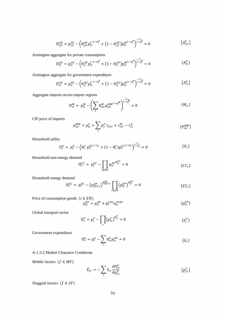
34

𝑖𝑗𝑟𝐴𝐹 = 𝑝𝑖𝑗𝑟

𝐴𝐹 (𝜃𝑖𝑗𝑟𝐴𝐹𝑝𝑖𝑟

𝑌 𝑖

+ (1 𝜃𝑖𝑗𝑟𝐴𝐹)𝑝𝑖𝑟

𝑀 𝑖

)

𝑖

= 0 {𝐴𝑖𝑗𝑟𝐹 }

Armington aggregate for private consumption

𝑖𝑟𝐴𝑃 = 𝑝𝑖𝑟

𝐴𝑃 (𝜃𝑖𝑟𝐴𝑃𝑝𝑖𝑟

𝑌 𝑖

+ (1 𝜃𝑖𝑟𝐴𝑃)𝑝𝑖𝑟

𝑀 𝑖

)

𝑖

= 0 {𝐴𝑖𝑟𝑃 }

Armington aggregate for government expenditure

𝑖𝑟𝐴𝐺 = 𝑝𝑖𝑟

𝐴𝐺 (𝜃𝑖𝑟𝐴𝐺𝑝𝑖𝑟

𝑌 𝑖

+ (1 𝜃𝑖𝑟𝐴𝐺)𝑝𝑖𝑟

𝑀 𝑖

)

𝑖

= 0 {𝐴𝑖𝑟𝐺 }

Aggregate imports across import regions

𝑖𝑟𝑀 = 𝑝𝑖𝑟

𝑀 (∑𝜃𝑖𝑠𝑟𝑀 𝑝𝑖𝑠𝑟

𝑀𝑀 𝑖𝑀

𝑠

)

𝑖𝑀

= 0 {𝑀𝑖𝑟}

CIF price of imports

𝑝𝑖𝑠𝑟𝑀𝑀 = 𝑝𝑖𝑠

𝑌 + ∑𝑝𝑗𝑇

𝑗

𝜏𝑗𝑖𝑠𝑟 + 𝜏𝑖𝑠𝑟𝑀 𝜏𝑖𝑠

𝑋 {𝑃𝑖𝑠𝑟𝑀𝑀}

Household utility

𝑟𝑈 = 𝑝𝑟

𝑈 (𝜃𝑟𝐶 𝑝𝑟

𝐸𝐶 𝐶 + 1 𝜃𝑟𝐶 𝑝𝑟

𝐶𝐶 𝐶)

𝐶 = 0 {𝑈𝑟}

Household non-energy demand

𝑟𝐶𝐶 = 𝑝𝑟

𝐶𝐶 ∏ 𝑝𝑖𝑟𝐴𝑃𝜃𝑖𝑟

𝐶𝐶

𝑖 𝐸𝐺

= 0 {𝐶𝐶𝑟}

Household energy demand

𝑟𝐸𝐶 = 𝑝𝑟

𝐸𝐶 (𝑝𝐸𝐿𝑌,𝑟𝐴𝑃 )

𝜃𝐸𝐿 ,𝑟𝐸𝐶

∏(𝑝𝑖𝑟𝐸𝑃)

𝜃𝑖𝑟𝐸𝐶

𝑖 𝐸𝑁

= 0 {𝐸𝐶𝑟}

Price of consumption goods 𝑖 𝐸

𝑝𝑖𝑟𝐸𝑃 = 𝑝𝑖𝑟

𝐴𝑃 + 𝑝𝑟𝐶𝑂2𝑎𝑖𝑟

𝐶𝑂2𝑃 {𝑝𝑖𝑟𝐸𝑃}

Global transport sector

𝑖𝑇 = 𝑝𝑖

𝑇 ∏(𝑝𝑖𝑟𝑌 )

𝜃𝑖𝑟

𝑟

= 0 {𝑌𝑖𝑇}

Government expenditure

𝑟𝐺 = 𝑝𝑟

𝐺 ∑𝜃𝑖𝑟𝐺𝑝𝑖𝑟

𝐴𝐺

𝑖

= 0 {𝐺𝑟}

A-1.3.2. Market Clearance Conditions

Mobile factors 𝑓 𝑀𝐹

�̅�𝑓𝑟 = ∑𝑌𝑖𝑟 𝑖𝑟

𝑌

𝑝𝑓𝑟𝐹

𝑖

{𝑝𝑓𝑟𝐹 }

Sluggish factors 𝑓 𝐹

35

�̅�𝑓𝑟 = 𝑇𝑓𝑟𝑆𝐹 {𝑝𝑓𝑟

𝐹 }

Sector specific sluggish factors 𝑓 𝐹

𝑇𝑓𝑟𝑆𝐹

𝑓𝑟𝑆𝐹

𝑝𝑓𝑖𝑟𝑆𝐹 = 𝑌𝑖𝑟

𝑖𝑟𝑌

𝑝𝑓𝑖𝑟𝑆𝐹 {𝑝𝑓𝑖𝑟

𝑆𝐹 }

Output

𝑌𝑖𝑟 = ∑𝐴𝑖𝑗𝑟𝐹

𝑗

𝑗𝑟𝐴𝐹

𝑝𝑖𝑟𝑌 𝐴𝑖𝑟

𝑃 𝑖𝑟

𝐴𝑃

𝑝𝑖𝑟𝑌 𝐴𝑖𝑟

𝐺 𝑖𝑟

𝐴𝐺

𝑝𝑖𝑟𝑌 ∑𝑀𝑖𝑠

𝑠

𝑖𝑠

𝑀

𝑝𝑖𝑟𝑌 𝑌𝑖

𝑇 i

𝑇

𝑝𝑖𝑟𝑌 {𝑝𝑖𝑟

𝑌 }

Sector specific energy aggregate

𝐸𝑖𝑟 = 𝑌𝑖𝑟 𝑖𝑟

𝑌

𝑝𝑖𝑟𝐸 {𝑝𝑖𝑟

𝐸 }

Import aggregate

𝑀𝑖𝑟 = ∑𝐴𝑖𝑗𝑟𝐹

𝑖𝑟𝐴

𝑝𝑖𝑟𝑀

𝑗

𝐴𝑖𝑟𝑃

𝑖𝑟𝐴𝑃

𝑝𝑖𝑟𝑀 𝐴𝑖𝑟

𝐺 𝑖𝑟

𝐴𝐺

𝑝𝑖𝑟𝑀 {𝑝𝑖𝑟

𝑀}

Armington aggregate for intermediate inputs

𝐴𝑖𝑗𝑟𝐹 = 𝑌𝑗𝑟

𝑗𝑟𝑌

𝑝𝑖𝑗𝑟𝐴𝐹 {𝑝𝑖𝑗𝑟

𝐴𝐹}

Armington aggregate for government expenditure

𝐴𝑖𝑟𝐺 = 𝐺𝑟

𝑟𝐺

𝑝𝑖𝑟𝐴𝐺 {𝑝𝑖𝑟

𝐴𝐺}

Armington aggregate for private consumption

𝐴𝑖𝑟𝑃 = 𝐶𝐶𝑟

𝑟𝐶𝐶

𝑝𝑖𝑟𝐴𝑃 {𝑝𝑖𝑟

𝐴𝑃}, 𝑖 𝐸𝐺

𝐴𝑖𝑟𝑃 = 𝐸𝐶𝑟

𝑟𝐸𝐶

𝑝𝑖𝑟𝐴𝑃 {𝑝𝑖𝑟

𝐴𝑃}, 𝑖 𝐸𝐺

Household utility

𝑈𝑟 = 𝑝𝑟𝑈𝐻𝑟 {𝑝𝑟

𝑈}

Aggregate household energy consumption

𝐸𝐶𝑟 = 𝑈𝑟

𝑟𝑈

𝑝𝑟𝐸𝐶 {𝑝𝑟

𝐸𝐶}

Aggregate household non-energy consumption

𝐶𝐶𝑟 = 𝑈𝑟

𝑟𝑈

𝑝𝑟𝐶𝐶 {𝑝𝑟

𝐶𝐶}

Government expenditure

𝐺𝑟 = 𝑝𝑟𝐺𝐻𝑟

𝐺 {𝑝𝑟𝐺}

Global transport service

36

𝑌𝑖𝑇 = ∑ 𝜏𝑖𝑗𝑟𝑠

𝑗,𝑟,𝑠

𝑀𝑗𝑟𝑠 {𝑝𝑖𝑇}

Price of emissions permit

𝐶𝑂2𝑟 = ∑𝐸𝑖𝑟

𝑖𝑟𝐸

𝑝𝑟𝐶𝑂2

𝑖

𝐸𝐶𝑟

𝑟𝐸𝐶

𝑝𝑟𝐶𝑂2 {𝑝𝑟

𝐶𝑂2}

A-1.3.3. Income.

Income of the representative household

𝐻𝑟 = ∑𝑝𝑓𝑟𝐹 �̅�𝑓𝑟

𝑓

+ 𝑝𝐶𝐺𝐷,𝑟𝑌𝐶𝐺𝐷,𝑟 + 𝑝𝑈𝑆𝐴𝐶 𝐵𝑟 𝑝𝑟

𝐶𝑇𝑟𝐿 {𝐻𝑟}

Government income

𝐻𝑟𝐺 = 𝑝𝑟

𝐶𝑇𝑟𝐿 + 𝑉𝑟

𝑅+BA tariff revenue – BA export rebate (subsidy) {𝐻𝑟𝐺}

Lump-sum transfer (tax) to household

𝐺𝑟 = �̅�𝑟 {𝑇𝑟𝐿}

Permit revenue

𝑉𝑟𝑅 = 𝑝𝑟

𝐶𝑂2 𝐶𝑂2̅̅ ̅̅ ̅̅𝑟 {𝑉𝑟

𝑅}

A-1.3.4. Equations for border adjustment

BA import tariff rates (BID, BIED, BIDR, BIEDR)

𝜏𝑖𝑠𝑟𝑀 = 𝑝𝑟

𝐶𝑂2𝜉𝑖𝑟 {𝜏𝑖𝑠𝑟𝑀 }

BA import tariff rates (BIF)

𝜏𝑖𝑠𝑟𝑀 = 𝑝𝑟

𝐶𝑂2𝜉𝑖𝑠 {𝜏𝑖𝑠𝑟𝑀 }

BA export rebate (subsidy) rates (BIED and BIEDR)

𝜏𝑖𝑟𝑋 = 𝑝𝑟

𝐶𝑂2𝜉𝑖𝑟 {𝜏𝑖𝑟𝑋 }