a case study of continuity, discontinuity and variability in early ...

Infant and Child DevelopmentInf. Child Dev. 16: 7–33 (2007)

Published online in Wiley InterScience

(www.interscience.wiley.com) DOI: 10.1002/icd.506

Wobbles, Humps and Sudden Jumps:A Case Study of Continuity,Discontinuity and Variability inEarly Language Development

Marijn van Dijka,* and Paul van Geertb

a Open University of the Netherlands, The Netherlandsb University of Groningen, The Netherlands

Current individual-based, process-oriented approaches (dynamicsystems theory and the microgenetic perspective) have led to anincrease of variability-centred studies in the literature. The aim ofthis article is to propose a technique that incorporates variabilityin the analysis of the shape of developmental change. Thisapproach is illustrated by the analysis of time serial languagedata, in particular data on the development of preposition use,collected from four participants. Visual inspection suggests thatthe development of prepositions-in-contexts shows a character-istic pattern of two phases, corresponding with a discontinuity.Three criteria for testing such discontinuous phase-wise changein individual data are presented and applied to the data. Theseare: (1) the sub-pattern criterion, (2) the peak criterion and (3) themembership criterion. The analyses rely on bootstrap andresampling procedures based on various null hypotheses. Theresults show that there are some indications of discontinuity inall participants, although clear inter-individual differences havebeen found, depending on the criteria used. In the discussion wewill address several fundamental issues concerning (dis)conti-nuity and variability in individual-based, process-oriented datasets. Copyright # 2007 John Wiley & Sons, Ltd.

Key words: intra-individual variability; early language develop-ment; continuity; discontinuity; random sampling techniques;dynamic systems theory; microgenetic

��

One of the major achievements of individual-based, process-oriented approaches(dynamic systems theory and the microgenetic perspective) is the increase in thenumber of variability-centred studies that have appeared in the literature. Theimplication is that a growing number of researchers acknowledge the mean-ingfulness of intra-individual variability and show an interest in irregular aspects of

*Correspondence to: Marijn van Dijk, Open University of the Netherlands, TheNetherlands. E-mail: [email protected]

Copyright # 2007 John Wiley & Sons, Ltd.

change. In line with these approaches, we have proposed to view developmentaldata as ranges of levels (see van Geert and van Dijk, 2002). These ranges are relevant,since they provide us with information on the flexibility and sensitivity of a systemto its environment. Where the maximal value represents the maximal performanceof a child under optimal circumstances, the minimal value indicates the vulnerabilityof this performance to other (less optimal) conditions. This flexibility andvulnerability might be different for different individuals or for the same individualat a different measurement occasion, i.e. for different phases in development. In thisarticle we will take the argument a step further by proposing a technique thatincorporates variability in the analysis of the shape of developmental change asdescribed in microgenetic and dynamic systems studies.

Developmental change can literally take many shapes, ranging from themonotonous increase of an underlying continuous curve to a pattern of ranges orpatches of variability. One important distinction among these different shapes ofdevelopment concerns the difference between continuity and discontinuity.Discontinuities are of special interest because they may indicate increasing self-organization in the system, that is, a spontaneous organization from a lower levelto a higher level of development (van Geert, Savelsbergh, & van der Maas, 1999).

In this paper, we argue for the incorporation of variability in the analysis ofdiscontinuity. The focus will be on methodological aspects, more specifically theuse of resampling techniques and various null-hypotheses of (dis)continuity. Aswe will demonstrate, results differ depending on the definitions and exactcalculation methods employed. This article should therefore be seen as a generalclaim for a move towards an ‘exploratory’ type of statistics. Instead of holding onto a single analysis technique, we advocate the need to explore a series ofstatistical models that are tested with resampling procedures. Also, instead ofperceiving continuity and discontinuity as a dichotomy, we argue that they mightbe conceived of as two extremes of one continuum. On this continuum,intermediate positions are possible, with the implication that a pattern mighthave some aspects of continuity and some aspects of discontinuity. Our final aimis to contribute to a better analysis and description of microgenetic data,including those collected within the framework of dynamic systems.

Continuity and Discontinuity

Although the meaning of the terms ‘continuity’ and ‘discontinuity’ differs acrossstudies, a general definition of discontinuity is provided by van Geert et al.,(1999): ‘we can define a discontinuity in the most general sense by identifying itwith a stage transition. That is, if a stage is replaced by another stage, in the senseof consecutive sets of different equilibria, a discontinuity has occurred’ [pp. XV].In a discontinuity the growing variable jumps from one level (or stage) to the nextwithout intermediary points. In practice, however, such a discontinuous curve ishard to distinguish from a (very) steep continuous curve. The reason for this isthat the empirical data sampling is almost by definition discrete and thus easilymisses points that lie along the steep increase. Thus, although the empiricalrepresentation of a developmental curve may show a discontinuity in the form ofa lack of intermediary points during a sudden jump or increase, it is notautomatically implied that the data refer to a discontinuous underlying process(see Figure 1). Figure 1(a) represents a continuous sigmoid curve of the formy¼ 1/(time+Exp(�(t�0.5)/0.001)). On a scale from 0 to 1, it shows a (seeming)discontinuity, however, a ‘magnification’ of the time scale (below) shows that the

M. van Dijk and P. van Geert8

Copyright # 2007 John Wiley & Sons, Ltd. Inf. Child Dev. 16: 7–33 (2007)DOI: 10.1002/icd

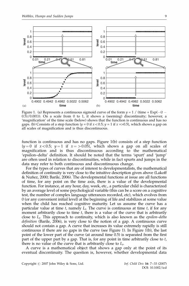
function is continuous and has no gaps. Figure 1(b) consists of a step function{y¼ 0 if x50.5; y¼ 1 if x¼40.05}, which shows a gap on all scales ofmagnification and is thus discontinuous according to the mathematical‘epsilon–delta’ definition. It should be noted that the terms ‘spurt’ and ‘jump’are often used in relation to discontinuities, while in fact spurts and jumps in thedata may refer to both continuous and discontinuous change.

For the types of curves that are of interest to developmentalists, the mathematicaldefinition of continuity is very close to the intuitive description given above (Lakoff& Nunez, 2000; Barile, 2006). The developmental functions at issue are all functionsof time, for any point on the time axis, there is a value of the developmentalfunction. For instance, at any hour, day, week, etc., a particular child is characterizedby an average level of some psychological variable (this can be a score on a cognitivetest, the number of complex language utterances recorded, etc), which evolves from0 (or any convenient initial level) at the beginning of life and stabilizes at some valuewhen the child has reached cognitive maturity. Let us assume the curve has aparticular value at time t, namely Lt. The curve is continuous at time t, if for anymoment arbitrarily close to time t, there is a value of the curve that is arbitrarilyclose to Lt. This approach to continuity, which is also known as the epsilon–deltadefinition (Barile, 2006), is very close to the notion of a gap. A continuous curveshould not contain a gap. A curve that increases its value extremely rapidly is stillcontinuous if there are no gaps in the curve (see Figure 1). In Figure 1(b), the lastpoint of the lower part of the curve (at around time 0.5) is separated from the firstpart of the upper part by a gap. That is, for any point in time arbitrarily close to t,there is no value of the curve that is arbitrarily close to Lt.

A curve is a mathematical object that shows a gap only at the point of itseventual discontinuity. The question is, however, whether developmental data

0 0

0.2 0.2

0.4 0.4

0.6 0.6

0.8 0.8

1 1

0.01 0.010.21 0.210.41 0.410.61 0.610.81 0.81time time

leve

l

leve

l0 0

0.2 0.2

0.4 0.4

0.6 0.6

0.8 0.8

1 1

0.4902 0.49020.4942 0.49420.4982 0.49820.5022 0.50220.5062 0.5062time time

leve

l

leve

l

(b)(a)

Figure 1. (a) Represents a continuous sigmoid curve of the form y = 1 / (time + Exp(�(t �0.5)/0.001)). On a scale from 0 to 1, it shows a (seeming) discontinuity; however, a‘magnification’ of the time scale (below) shows that the function is continuous and has nogaps. (b) Consists of a step function {y = 0 if x50.5; y = 1 if x =>0.5}, which shows a gap onall scales of magnification and is thus discontinuous.

Wobbles, Humps and Sudden Jumps 9


can be validly described in the form of curves that eventually show the type ofdiscontinuity described by the gap criterion. To put it differently, are (underlying)curves indeed the descriptive format that developmentalists wish to extract fromtheir data and, if they are not, is the standard gap definition of discontinuity stillapplicable to those data? Before answering this question, let us first take a closerlook at an important property of developmental data, namely their variabilitywithin individuals.

Variability

In van Geert and van Dijk (2002), we have defined intra-individual variability as‘differences in the behaviour within the same individuals, at different points intime’ (pp. 341). In quantitative developmental data, intra-individual variability isexpressed as fluctuations between measurement points. Variability has largelybeen neglected until the introduction of dynamic systems and microgeneticperspectives. Both take a radical departure from the traditional approach tovariability. This traditional view is voiced by a strong axiom in psychology called‘true score theory’, which considers variability to be the result of measurementerror (Cronbach, 1960; Lord & Novick, 1968; Nunnally, 1970). Dynamic systemstheory and the microgenetic approach, on the other hand, claim that variability isdevelopmentally meaningful and bears important information about the natureof the developmental process. For instance, Thelen and Smith (1994) explain that,in a self-organizing process, behavioural variability is an essential precursor of anattractor state (one preferred configuration out of many possible states). Theystate: ‘Variability is revealed when systems are in transition, and when theyundergo these shifts, the system is free to explore new and more adaptiveassociations and configurations’ (pp. 145). Thelen and Smith encourageresearchers to investigate the variability in their data. Inspired by this newdefinition, several studies have been performed that adopt Thelen and Smith’ssuggestion, they treat variability as data, and analyse it (for instance Bertenthal,1999; Bertenthal and Clifton, 1998; de Weerth and van Geert, 1999, 2002; Newelland Corcos, 1993). Variability also features in the microgenetic approach. Thisfocus on variability is shown, among others, in the work of Siegler (1994, 1996,1997), Goldin-Meadow, Alibali, and Church (1993), Alibali (1999), Granott (1993),Fischer and Granott (1995), Fischer, Bullock, Rotenberg, and Raya (1993), Fischerand Yan (2002), Lautrey, Bonthoux, and Pacteau (1996), Lautrey (1993), Lautreyand Cibois (1994), Tunteler and Resing, (2002), Granott (1998, 2002), Pine, Lufkin,and Messer (2004) and Flynn, O’Malley, and Wood (2004).

The reason that we look at variable data is that we want to learn somethingabout the causes of the observed phenomena. We agree with Miller (2002) thatvariability in cognitive performance can provide insight into the process, or‘generator’, of change. The classical view is that the generator is a dedicatedinternal generator, with specific properties. For instance, in the case of developingintelligent behaviour, such a generator may be a ‘device’ or ‘module’ in the brainwith a certain strength or ‘power’ that produces cognitive behaviour. In theclassical view, the actual product (e.g. the score on a cognitive test) is caused bythe internal generator (the ‘device’) plus a number of additional mechanisms orvariables that randomly intervene with the working of the actual generator.Classical test theory aims at measuring the power of the cognitive device, andsees the additional variables as sources of measurement error. Dynamic systemstheory, on the other hand, proposes the notion of a distributed generator that



consists of all the factors or agents that causally contribute to the production ofthe observed variable at issue at a particular time and place. This generatorparticipates in a developmental process. This implies that in our example, a scoreon a cognitive test is the product of the mutual and complex interaction betweenthe capacities of the child and the context.1

The way a researcher looks at the nature of the data is closely related to theway he or she looks at the nature of the generator. The notion of an internal,dedicated generator mechanism implies that the observed data are the product ofthe generator plus a number of accidental influences. Thus, according to thisbelief, in order for the data to teach us something about the progress of theunderlying generator, the errors must be disposed of, which in all likelihood willresult in a smooth curve that corresponds with the assumed real level and changeof the underlying generator. From a dynamic systems point of view, however, thegenerator is a complex process itself, the properties of which are represented,among others, in the way it fluctuates over time. Thus, the fluctuations are part ofthe information that the data can give us about the nature of the generator andtherefore an analysis of these fluctuations is of central importance.

In the next section, we will present examples of microdevelopmental studies inwhich the issue of continuity versus discontinuity plays an important role anddiscuss the contribution of catastrophe theory.

Discontinuities in Developmental Studies

The question as to whether a developmental process is continuous ordiscontinuous is a relevant problem in (micro)developmental studies. Let usdiscuss an example from Fischer and Granott (1995). Their study consisted of theproblem solving interaction of dyads learning to understand an unfamiliardevice. One striking example of a particular dyad showed that there was aninitial low level of understanding in both individuals, then a clear progression,which was characterized as ‘. . .non-linear, dynamic microdevelopment, with upand down oscillations, gradually moving to increasing complex interactions andrepresentations’ (p. 309). In short, the microdevelopmental pattern shows achange in the range across which the oscillations occur. It remains to be tested,however, whether this change is indeed gradual (continuous), or discontinuous.

As a second example, let us consider the balance scale tasks of Siegler and hiscolleagues (see Siegler & Chen, 2002). These balance scale tasks are often seen as abenchmark for the testing of the usefulness of various methodological andtheoretical approaches in cognitive development. A recurrent finding of thesestudies is that a large majority of 5-year-olds consistently use rules to solvebalance scale problems, while 3-year-old children rarely use rules systematically.Balance scale rules are ordered hierarchically. At first children use predictionsonly based on weight (Rule I), then only based on distance (Rule II), and finallythey combine both quantitatively (Rule III). However, while rule use correlateswith age, there exist obvious inter-individual and intra-individual differences.This means that variability (both inter-individual and intra-individual) is alsopresent in the performance on balance scale tasks. Siegler and his colleaguesemploy the typical criterion for concluding that a child used a given rule, that80% of the child’s responses on a large number of items are predicted by thatrule. The question remains how the frequencies of rule use develop. Is there agradual increase in rule use across trials?

According to Janssen and van der Maas (2002), there is empirical evidence thatat least one transition in the development of solving the balance scale



problem}from rule I to rule II}is discontinuous. The theoretical framework fortheir conclusion is based on catastrophe theory (Thom, 1975), which can beconsidered a specific branch of dynamic systems theory. According to this theory,self-organizational processes can be classified into a limited number ofcharacteristic patterns of discontinuous change, depending on the number offundamental variables that determine the change. As such, catastrophe theoryoffers concrete models and criteria for discontinuities in developmentalprocesses. All these catastrophes are discontinuities that are caused by changesin control variables (i.e. variables controlling the generator process that producesthe changes in the measured variable). Of these seven catastrophes, the cusp isthe simplest: it is controlled by two variables and there are two equilibriumstates. The cusp can be fitted directly to data consisting of measurements for x, yand z (Cuspfit, Hartelman, 1996, based on the method of Cobb & Zachs, 1985).A second way of testing the cusp catastrophe model uses the qualitativecharacteristics of the cusp model. Catastrophe theory provides eight so-calledcatastrophe flags to test for the presence of a cusp model (Gilmore, 1981). Janssenand van der Maas (2002) have found evidence that the transition from rule I torule II is discontinuous in that it is characterized by four (out of five testable2)catastrophe flags.

The method of catastrophe testing has several drawbacks. First, the directfitting of a cusp catastrophe model is confined to data sets for which estimationsof the two control variables are available and thus, by implication, is limited tophenomena that critically depend on only two control variables. In manydomains of development, no real control parameters are available. However, themost serious problem with catastrophe testing is the fact that the underlyingmodel does not acknowledge the variability as true meaningful data. Instead, thecusp catastrophe model is in fact based on a point source model, in the sense thatthe source of development (the generator) corresponds with certain ‘true’ levelsof development, which can be represented as single values on a curve. Observedvariability across the trajectory is considered to be noise added to this pointsource. Hence, the catastrophe model provides no answer to the question of howdiscontinuity can be demonstrated in a phenomenon that is in essence a changein its range properties.

Discontinuity and Ranges

The phenomenon we deal with concerns the development of a distributedgenerator, as above. An example, discussed in the preceding section, is thedyadic generator producing a changing understanding of an unfamiliar device.Another example is the generator that produces the verbal and non-verbalreactions of a child to a balance-scale question. If it is the essence of aphenomenon that it appears as a score range (due to variability), the modelof this phenomenon should also be focused on that range, in such a waythat the model must describe this range as accurately as possible. Therefore wedefine a discontinuity as, ‘a transition from one variability pattern (range), to adifferent variability pattern, in the sense that these patterns are separatedby a gap’.

Adopting an individual-based approach, we formulate the following assump-tions. We may either have certain assumptions about the underlying nature of thisrange (for instance, that it can be described in terms of a normal}or someother}distribution), or we may assume that the best possible model of the range



are the range data themselves (this assumption comes close to the basicassumption of the bootstrap method in statistics, see Efron and Tibshirani, 1993).In the latter case, we should use this range without further ‘corrections’ (forinstance without the prior use of a smoothing procedure). In any case, the mainquestion, which we introduced earlier, must now be answered: how can the gap-criterion of discontinuity (the epsilon–delta criterion of mathematics) be appliedto discontinuities in ranges?

To begin with, time-serial data from developmental studies consist of sets ofseparate data points. That is, there are gaps everywhere. Does it make sense toapply the gap definition to something where gaps are everywhere? The trick is toconsider a set of developmental, time-serial data as a single object, which in thiscase is the range. Continuity can be defined as set-membership, as belonging tothe range. Any two data points within the range are, by definition, continuous.Any two data points, one of which lies in the range and one of which lies not inthe range, are by definition, discontinuous. The set of observed data points is ofcourse just a small subset of all the possible points that could lie within the range.Thus, how do we decide whether a particular, new data point, lies in the range ornot?

To make this decision we envisage an imaginary magic bug that can jump fromany point in the range to any other one, but cannot do anything else. Thus, therange is in fact defined by the set of possible jumps the magic bug can make,whatever point lies within the bug’s radius of action is a potential member of therange. Let us proceed by adding a new data point to the series, in this case a newmeasurement of some developing variable. Does this new data point correspondto a continuity or a discontinuity? We can ask the bug. If he has a jump in hisrepertoire that can bring him from anywhere in the range to the new point orbeyond, there is no gap from the bug’s point of view between the range and thenew point. Thus, the new point is continuous to the range. If he has no such jumpin his repertoire, and thus cannot reach the new data point from somewhere inthe range, there is a gap from his point of view, and the new data point is adiscontinuity. The magic bug metaphor maps directly onto a mathematicaldefinition of (dis)continuity in ranges defined by sets of data points. Central tothe argument is the definition of a range of data points by the set of possible‘jumps’ from one point to another within the range.

Figure 2 represents the temporal layout of a range across the time dimension.The new data point, at time 30, can have three values: (a), (b) or (c). Position (a)belongs to the range by definition. In order to determine the degree-of-membership of values (b) and (c), we need the range layout and the magic bugthat defines the range of the set of the ‘possible jumps’. Position (b) lies within therange of the bug’s jumps, and its degree-of-membership is greater than 0 butsmaller than 1. Position (c) cannot be reached by the jumping magic bug: thereremains a gap between the bug’s furthest position and position (c), (c) has adegree-of-membership of 0, and thus indicates a discontinuity at time 30.

In the remainder of this article we will demonstrate an approach to analyse(dis)continuity in developmental processes using the concept of developmentalranges. This approach is based on the exploratory use of resampling techniques,and shows the application of various statistical models of discontinuity to data ofearly language development. A further characteristic of discontinuity indevelopmental data is that it can take various forms, depending on the type ofdevelopmental process we are dealing with. Thus, the empirical criteria ofdiscontinuity will vary with the type of process under study. However, they willall boil down to some form of anomaly that marks a point of transition. In the



next section, we will introduce our case study. The discontinuity criteriaapplicable to this particular case will be presented in the method section.

Illustration: a Case Study on (dis)continuity in the Development of EarlyPrepositions

In this article, we will demonstrate the application of several criteria to test fordiscontinuities in a particular empirical example. This consists of the question ofwhether the acquisition of early prepositions-in-contexts shows discontinuouscharacteristics. Both issues (variability and discontinuity) are related to an importanttheme in the acquisition literature. Language development is often characterized interms of stages or phases (for instance, in the case of Dutch, see Fikkert, 1998; vander Stelt & Koopmans-van Beinum, 2000; van Kampen & Wijnen, 2000). Thequestion remains as to whether these stages are merely descriptive characterizationsor whether they are true discrete stages (a sequence of periods in time with coherentelements that have a certain degree of stability), with discontinuous transitions.

In the language acquisition literature, there are only a handful of studies thatexplicitly report quantitative data on the developmental trajectory of preposi-tions. Interestingly, these suggest that this process might be stage-wise. Forexample, in his classic case-study Brown (1973) describes that initially, Eveomitted the prepositions ‘in’ and ‘on’ (in so-called ‘obligatory’ contexts) morethan she supplied them. However, from the seventh measurement onwards,prepositions were constantly supplied in 90–100% of all obligatory contexts.

0

2

4

6

8

10

12

14

16

15 20 25 30

time

leve

l

rang

e

gap

a a

b b

c c

temporal lay-out range lay-out

(a) (b)

Figure 2. (a) The range covered by the hatched rectangle is continuous at time 30: themeasurement at time 30 can be ‘reached’ from the range and there is no gap. (b) Thehatched range is discontinuous at time 30: the measurement made at time 30 cannot be‘reached’ from the range, hence, there is a gap at time 30 (for a formal definition of‘reachability’, see text).



Stenzel (1996) revealed a similar jump-wise pattern in a bilingual child. In thebeginning, prepositions were only used very infrequently. He states, ‘[I]n the firstphase, the absolute number of tokens is very low, and we find some strangedistributions. In the second phase, the number of utterances containingprepositions is rather high in some recordings (and zero in others); and thepattern observed in the first phase vanishes.’ [pp. 1036]. Thus, while thequantitative development of prepositions might be stage-wise, it is unknownwhether the transition between these stages is discontinuous.

The issue of continuity versus discontinuity in the development of theseprepositions-in-contexts can be approached from different theoretical stand-points. In the case of continuity there might be a gradual differentiation: from arestricted use to a more refined and flexible application of prepositions in avariety of distinct contexts. In this case, the child acquires the new prepositionscontext-by-context or type-by-type. From one conceptual standpoint, continuitycan be expected if the order of acquisition follows the underlying conceptualcomplexity of prepositions (Clark, 1978; Johnston & Slobin, 1979), that is, if theacquisition of the related non-linguistic spatial knowledge is continuous. Fromthe modular point of view, continuity can also be expected, as the result of themapping of spatial concepts between three main cognitive modules, namelyperception, action and language (van Geert, 1986). In the case of a discontinuouscurve, the child suddenly discovers the way prepositions can be used to labelspatial relations between objects. This discovery might function as a threshold,after which prepositions are used in abundance, while before their use havingbeen seldom, and only in verb-like situations. A discontinuous trajectory isexpected if, for instance, the required syntactic rules are acquired, and these rulesgeneralize instantly across types and contexts. Here, the discontinuity stems fromthe sudden acquisition of a new structural category, namely the syntactical use ofprepositions. This may lead to an instantaneous application of the prepositioncategory to a wide collection of spatial contexts. However, while the question ofcontinuity and discontinuity is certainly relevant, language has primarily beenchosen as an exemplary data set to demonstrate the application of our methods.Our aim is to lay out a procedure for investigating variability and discontinuityin an integrated fashion. This procedure is applicable to a wide variety ofdevelopmental processes. In this sense, there is no difference between languagedevelopment and other aspects of cognitive development such as cognitive skills(e.g. Fischer & Yan, 2002), strategy change in solving mathematical problems (e.g.Alibali, 1999), or scores on a balance scale test (e.g. Jansen & van der Maas, 2002).

METHODS

The Data set

In the present case study, four participants (Heleen, Jessica, Berend and Lisa)were followed over the course of a year from around age 1 year and 6 months toage 2 years and 6 months. At the beginning of the study, the infants werepredominantly at the one-word stage, while at the end of the observation periodtheir language showed various characteristics of the differentiation stage. At thisstage, children generally acquire, besides the major lexical categories (such asnouns, verbs adjectives/adverbs), the word classes that have a primarysyntactical function (such as articles, pronouns, prepositions). Also, childrenlearn to use morphological and syntactical rules and, as a result, their sentences



become longer and more complex. As an example, in the differentiation stagechildren, start using verb inflections (for a detailed description of thecharacteristics of the Dutch differentiation stage, see Gillis & Schaerlaekens,2000). The participants were raised in a monolingual Dutch environment, with noapparent dialect. The children’s general cognitive development was tested withthe Bayley Developmental Scales 2/30 (van der Meulen & Smrkovsky, 1983) afew months before their second birthday. The scores were average to aboveaverage. All participants came from middle class families, who lived in suburbanneighbourhoods in average to large cities in the Netherlands. For details on theparticipants, see Table 1.

The study is based on videotaped observations of spontaneous speech undernaturalistic circumstances (the child’s home). (For further details on thedata collection and measurement design see van Geert & van Dijk, 2002).For the analysis of the speech samples, the child’s utterances that contained apreposition were transcribed orthographically according to Childes conventions(MacWhinney, 1991). This was done by an experienced transcriber (the firstauthor or intensively trained graduate students, one student per infant). Inter-observer reliability was calculated as the positive overlap ratio on the basis of anutterance-by-utterance comparison of a series transcripts out of a random sub-sample of the total data set. The resulting positive overlap ratios were 0.84(Heleen), 0.88 (Jessica), 0.87 (Berend) and 0.87 (Lisa), which is considered to beadequate.3 All prepositions that belong to the set of spatial prepositions wereselected, but only if the context was spatial. The total set of spatial prepositionsconsisted of ‘in’, ‘uit’, ‘op’, ‘af’, ‘voor’, ‘achter’, ‘tussen’, ‘over’, ‘bij’, ‘naar’, ‘onder’,‘boven’, ‘binnen’, ‘buiten’, ‘door’ (approximate translations are in, out, on, off,before/in front of, after/behind, between, over, near (to)/at, to/by, to, under,above, in/inside, out/outside, through). We counted the total frequency ofprepositions that were uttered in a particular spatial context. All distinct spatialcontexts were counted, excluding exact repetitions.

The Analyses

The analyses are based on individual trajectories, and consist of bootstrap andresampling procedures (for general discussions of these methods, see for instanceGood, 1999, Manly, 1997; the procedures were carried out in Microsoft Excel, bymeans of a statistical add-in, Poptools, Hood, 2001). The question we address is:do the individual trajectories show discontinuities in the developing range?

Criteria of DiscontinuityThe concept of discontinuity we adopted in this study is ‘a transition from one

variability pattern (range), to a different variability pattern, in the sense that thesepatterns are separated by a gap’, a definition that assigns a central position to

Table 1. Participant characteristics

Name Ages Number of Observations Gender

Heleen 1;6,4–2;5,20 55 FemaleJessica 1;7,12–2;6,18 52 FemaleBerend 1;7,14–2;7,13 50 MaleLisa 1;4,12–2;4.12 48 Female



variability. Therefore, our testing criteria are designed to be sensitive to changesin these variability patterns. The question we intend to answer by means of theseprocedures is, to what extent is a continuous model capable of producing theranges of our four participants. This question can be reformulated as, to whatextent do we need a discontinuous model to produce the data of our fourparticipants? The smaller the probability that a continuous model (plus randomvariability) reproduces our data, the less likely it is that the observed differencesin our four participants are an accidental outcome of an undivided, continuousdevelopmental trajectory.4

The Null-hypothesesThe null-hypotheses are based on various continuous models. These are,

respectively, a (1) linear and (2) quadratic model on the one hand and non-linearmodels with symmetric noise based on (3) Loess smoothing or (4) moving averagesmoothing of the data on the other hand. Each of these models follows the trend inthe data in a continuous fashion. In line with the continuity-hypothesis,variability is considered as noise. Consequently, for each of these models, anoise component was estimated by fitting a regression model to the residuals (thedifferences between the observed values and the values estimated by thecontinuous curves). The regression model specifies the expected variance of thenoise for each point in time, under the assumption that the noise follows anormal distribution. A continuous null hypothesis model can thus be simulatedby adding a Gaussian noise component to any point of the estimated continuouscurve. We will proceed as follows, first, the continuous models will be estimatedon the basis of characteristics of the observed data. Then, these models are usedto simulate data sets. Each of these simulated data sets will therefore, bydefinition, be produced by the continuous model. If these simulated models arecapable of producing the statistical indicators of discontinuity that we observedin our participants, the null-hypothesis of underlying continuous developmentcannot be rejected. It is also possible to perform a meta-(resampling)analysis tothis data, but since our approach is individual-based, our emphasis is on theindividual curves.

The CriteriaIn this study, we looked for three indicators that are likely to occur in any kind

of discontinuity. The first is the existence of two clearly distinct sub-phases orsub-patterns. If a discontinuity occurs, it is likely to be evident in the form of twodistinct sub-patterns, e.g. distinct patterns of data in terms of distinct scoreranges. The question is, what is the probability that the sub-patterns that wethink correspond with a discontinuity, in fact result from a continuous modelwith symmetrical noise. The second indicator is the existence of an anomaly in thedata at the moment of the discontinuous shift. We expect that such an anomalycan be observed in the form of an unexpectedly large, local peak or ‘spike’ in thedata. The peak results from the (presumed) sudden emergence of some new form(rules governing the use of spatial prepositions). In addition, there is a fair chancethat new forms are likely to be abundantly used right after their initial discovery(a sort of novelty effect). Finally, the third indicator is based on the assumptionthat the discontinuity corresponds with the fact that the data consist of twodiscontinuous sets of scores, expressed in terms of degrees-of-membershipto a set. Referred to as the gap criterion, this is defined by the analogy of themagic bug.



The use of three different operationalizations of discontinuity and of four nullhypothesis models is inspired by the method of converging evidence. The morethe criteria converge on the finding of a discontinuity in an individual trajectoryat the same point in time, the more credibility is given to the conclusion that thediscontinuity is real. The choice of our exploratory procedures and the principleof convergent evidence do not necessarily imply that the proposed set of criteriaand models is exhaustive or sufficient. Other developmental phenomena mightrequire discontinuity criteria that are eventually better adapted to the particularnature of the phenomenon in question. Starting from the idea of convergingevidence, we have taken the definitions of discontinuity that we have providedabove as a reasonable starting point, assuming that their transformations intotestable criteria provide us with a sufficient answer to the question whether ornot our data show discontinuous changes.

Criterion 1: Significantly Different Sub-patterns

The definition of a discontinuity was formulated above stated, ‘a transition fromone variability pattern (range), to a different variability pattern, in the sense thatthese patterns are separated by a gap’ (see Figures 1 and 2). The first and strictestdefinition of discontinuity requires the search for two distinct variability patternsand assumes a model of two clearly discernible phases that can be characterizedas two distinct series. On the other hand, if the null-hypothesis of continuousdevelopment is true, the trajectories basically consist of a single undividedpattern. If this is the case, the observed frequencies with which prepositionsoccur will randomly fluctuate around a single, continuous trajectory. With suchrandom fluctuation, however, it is not unlikely that some arbitrary divisions ofthe entire data set in two subsets will result in sub-patterns that also show someapparent discontinuity, as defined by the different-sub-pattern criterion. Thecritical issue is, what is the probability that the continuous models with randomfluctuations produce a two-stage difference that is of the same magnitude as thetwo-stage difference found in our data? The smaller the probability, the less likelyit is that the observed distances in our four subjects are an accidental outcome ofan undivided and thus continuous developmental trajectory.

In various publications, Fischer has claimed that it is not possible to observediscontinuities in the developmental data if the data are based on what he callsthe ‘functional level’, which means the level of unsupported performance (seeFischer & Rose, 1994; Fischer & Yan, 2002). In order to discover eventualdiscontinuities, we must monitor the child’s optimal level of performance, whichis achieved by giving the child support. The discontinuities in that optimal level,if any occur, are indicators of stage-wise changes in the child’s performance.Although we cannot provide our participants with support, we can neverthelessobtain an estimation of their optimal preposition production by simply taking thelocal maximum of the preposition frequencies (the local maximum is themaximum value in a window of observations, in this case five consecutiveobservations).

Thus, by monitoring the change in local maximum levels, it is possible todemonstrate a discontinuity in the maximal values, in the use of spatialprepositions. However, we announced above to ‘investigate whether adiscontinuous transition from one variability pattern to a different variabilitypattern exists.’ If, by variability pattern we mean the width of the range withinwhich the use of spatial prepositions can vary from observation to observation,



the focus on maximal values cannot, by definition, be used to show that such adiscontinuity exists, simply because the maximal level alone is not an index ofvariability. Thus, we may think of a sudden shift in the distance between theextremes, as an indicator of the presence of two sub-stages.

Statistical ProcedureAs a measure for the maximum performance level, we took the Progressive

Maximum. This starts with the value of the first observation and then takes themaximum of a progressively widening window that expands from the second upto the last observation (see van Geert & van Dijk, 2002 for a description andjustification). In the same manner, for the local minimum, the RegressiveMinimum was calculated. The regressive minimum starts with the value of thelast observation and then takes the minimum of a progressively wideningwindow that expands from the last up to the first observation (see also van Geert& van Dijk, 2002). We now calculate the difference between the two extremes (thedifference between maximal and minimal performance) and take this as our keyvalue. We now divide the data series in two parts, taking all possible divisions(beginning with data point 1–5, compared to the rest of the data, i.e. 6 to last, then1–6 against 7 to last, and so forth). For each subset, we select the maximal keyvalues obtained. The difference between these two key values defines the maximaldistance between the two sub-patterns for this particular data subset. The placewhere the distances differ maximally from each other marks the position of theassumed discontinuity (see Figure 3).

This procedure is carried out for the original data set and compared with asimilar procedure for the data sets simulated on the basis of the continuous nullhypothesis models. This whole procedure of generating a simulated series andcalculating the maximal difference between the two subsets in the simulated datais repeated a great number of times (in this case 5000 times). Finally, we count thenumber of times the simulated continuous model has produced a maximal

0

5

10

15

20

25

30

-270 -220 -170 -120 -70 -20 300 80

time

freq

uen

cy

Figure 3. Data from Heleen show a potential discontinuity at time 0, based on theassumption that the range expands discontinuously at time 0.



difference between the subsets that is as big as or bigger than the maximaldifference between subsets that we have obtained from our observed data series.This number, divided by the number of simulations, gives us the p-value of theobserved difference under the null hypothesis as specified.

Criterion 2: The Peak Model

While Criterion 1 (see previous section) conceptualizes discontinuity in terms oftwo distinct variability patterns, the second criterion focuses on the aspect of the‘gap’ at moment of the transition. This gap might be conceptualized as a ‘suddenchange’ in the curve. Thus, with this criterion, we identify a discontinuoustransition if the trajectory shows an unexpectedly large peak or spike, at somepoint in time. This peak might reveal the moment at which the system loses itsstability and shifts into a different variability pattern. As mentioned earlier, thereis a fair chance that the sudden emergence of a new skill or ability ischaracterized by a (probably short) time of abundant use of that new skill orability. This transient performance peak, if any occurs, will be added to thesudden shift in the sub-patterns described in the previous section, and thusmarks the underlying transition even more clearly.

Statistical ProcedureWe conceptualize a peak as the maximal positive5 difference between an expected

and an observed value in the trajectory. With this criterion, we have defined apeak in two distinct ways: an absolute peak and a relative peak. In case of theabsolute peak, variability at a specific point in time is defined as the absolutedifference between the observed (or simulated) data point and the expectedpoint, based on the underlying continuous model. This difference is the residualvalue, which is used to define the absolute peak. In the case of the relative peak,these residuals (for all points in time) are divided by the expected value, i.e. thevalue of the continuous model at the corresponding point in time. We have madethe distinction between absolute and relative peaks because the degree ofvariability is often strongly related to the central tendency in a distribution. As anillustration, assume a trajectory that shows a simple increase from value 1 tovalue 50. In this example, a residual of 4 is considered to be more salient if itoccurs around an observation with value 5 if when it occurs around value 45.While the absolute peak is strictest and signals unexpected spikes in the data, therelative peak criterion is sensitive to smaller peaks that might be meaningful inthe context that they appear in.

In our statistical procedure, finally, we take the peak (the maximal value ofeither absolute or relative residual) in the data as our key value and test it againstthe peaks found on the basis of a great many (5000) simulated continuousmodels, with distribution characteristics similar to those of the data.

Criterion 3: Membership Procedure

Previously, we have postulated that if a discontinuity occurs, it shows itself in theform of two distinct sub-patterns. According to the epsilon–delta definition of(Barile, 2006), a curve is continuous at time t, if for any moment arbitrarily closeto time t, there is a value of the curve that is arbitrarily close to Lt. On the otherhand, a discontinuous curve contains a gap between the two stages or phases,



however close they are to each other in time. We have shown that this epsilon–delta or gap criterion can be generalized to data sets or ranges, by means of themagic bug metaphor. Formally speaking, the bug’s jumps define a set of data thatare within reach of the bug. That is, all data points within reach of the bug aremembers of the set and have a set or range membership equal to 1. Any new datapoint that is within reach of the bug’s repertoire of jumps are also members of theset, and those that are not within reach are not members of the set or range. Thethird criterion relates the existence of a gap to the concept of set membership thatstems from Fuzzy Logic (McNeill & Freiberger, 1993).

Fuzzy logic rests on the idea that all things are characterized by the degree towhich they are members of a class. In modern fuzzy logic, ‘objects’ (observations,objects, properties, etc.) are assigned a degree-of-membership to a particularcategory (see Ross, 1995, for a particularly clear technical introduction; seefurther Kosko, 1993, 1997; McNeill & Freiberger, 1993; Nguyen & Walker, 1997;von Altrock, 1995, provide a highly accessible introduction). In mutuallyexhaustive classes, objects have a degree-of-membership of either 1 or 0. Forinstance, a particular piece of furniture is either a chair or not a chair (forinstance, it is a bench). In fuzzy logic, an object can have any degree ofmembership between 0 and 1. For instance, the piece of furniture is a chair thatlooks like a bench, e.g. has a degree of membership of 0.8 to the category ‘chair’.Maximal ambiguity arises if an object has a degree of membership equal to 0.5. Inthis case, the object is 50% part of a category, and 50% not. According to themembership criterion, we conceive of the data set as either a single ‘set’, or as aseries of ‘sets’ (in principle two). All data values can be assigned a degree-of-membership to each set. In the simplest case, the case of continuity, the dataconsist of a single set, and thus all values in the data set, have a degree-of-membership of 1 to that set. If the data are truly discontinuous, the data are cutinto two consecutive sets if a new data point emerges that is not a member of theset of data points already present (say at time t). A data point belongs either tothe first or to the second set, thus a data point has a degree-of-membership of 1 tothe first set and 0 to the second set. Data points can also be somewhere inbetween and thus have a degree-of-membership of, for instance, 0.5 to the firstand 0.5 to the second set.

Statistical ProcedureSet membership is easy to define. Suppose that we define data points a, b, c to

m as members of a set S. Now we collect a new data point, n and wish to know ifit also belongs to the set. Recall that the magic bug defined set membership by itspossible jumps. A possible jump is for instance the jump from a to c, which is ajump of length |a–c|. Any member of the set is a possible starting point for thebug. Take for instance point f. Since all points that can be reached by the bug aremembers of the set, the point that lies at distance f � |a–c| is also a member ofthe set. The degree-of-membership of (potential) members of the set is defined asfollows. If f is the set’s maximal value, if |a–c| is the sets greatest distance and ifn lies not within reach of f �|a–c|, the degree-of-membership of n to the set S is 0.More precisely, there exists a gap between n on the one hand and the set S on theother hand.

All points that have been assigned to the set (i.e. a to m) have, by definition, adegree-of-membership of 1. All points that lie between any two possiblemembers of the set (e.g. a point lying between a and d) have, by implication, adegree-of-membership of 1. All other points have a degree-of-membership



which is equal to the likelihood that such points are within reach of the bug(lying within reach refers to the membership by implication: remember thatif a is a member and b is a member, a new point n is also a member if it liesbetween a and b). Thus, the degree-of-membership of n is defined by thesum of probabilities of all the possible ‘jumps’ for which n lies within reach. Sincea jump is defined mathematically as m1 � |m2–m3| (for m1, m2 and m3

arbitrarily chosen full members of the set), the degree-of-membership is definedby the sum of probabilities of such triplets. A practical way of calculatingdegrees-of-membership is by randomly sampling triplets of values from a dataset S, calculate the resulting m1 � |m2–m3| value and repeating that a greatmany times. By doing so we can numerically approximate the likelihood ofoccurrence of any possible value and thus determine its degree-of-membershipto the set.

The set S can be specified by taking an initial set (e.g. the first four to five datapoints, ranging from time t1 to t4), determine if the first data point outside the set(i.e. the point at time t5) is a member, add it to the set if its degree-of-membership issatisfactory (e.g. > 0:8; > 0:95 or whatever seems reasonable) and continue until wemeet a data point whose degree-of-membership is smaller than some pre-esta-blished value (in this case 0.05). This data point defines a discontinuity in the data.

RESULTS

Visual Inspection of the Developmental Curves

In order to get a general impression of the development of prepositions weplotted the trajectories of the four participants in Figure 4. On the basis of visualinspection, we aligned participants to their first major peak in their trajectories.Using this representation, all participants show their first major ‘jump’ at point

Lisa

38

1318232833

-177 -127 -77 -27 230 73 123 173time

freq

uen

cy

Heleen

0

5

10

15

20

25

-267 -217 -167 -117 -67 -17 33 83

time

freq

uen

cy

Berend

05

101520253035

-36 140 64 114 164 214 264 314

time

freq

uen

cy

Jessica

05

101520253035

-100 -50 0 50 100 150 200time

freq

uen

cy

0

Figure 4. The individual trajectories of prepositions-in-context, Heleen, Jessica, Lisa andBerend.



zero on the x-axis. The other numbers on the axis represent the number of daysbetween the other observations and this point zero.

Visual inspection of the individual trajectories shows that most participantscan be described in terms of two distinct phases. First, they show a period inwhich prepositions-in-context only occur occasionally, usually the phase beforepoint zero. In this phase, prepositions fluctuate mildly between values lower than10. As an exception, Lisa’s initial values reach around 15. Then, further on, alltrajectories are characterized by strong fluctuations, which occur after the firstmajor outbursts of prepositions. Inter-individual differences are clearly visible.For instance, the timing of the transition between this first and second phasediffers between the four participants. While Heleen shows a relatively long initialphase, Berend only shows seven values that might be characterized as such. Itcan be questioned whether Berend actually displays the initial phase wedescribed above. However, since we have no data before measurement point�38, we can only speculate on the existence of a first phase as found in the otherparticipants.

Thus, solely on the basis of visual inspection, trajectories of these fourparticipants may be described in terms of two distinct phases. First, there is aninitial phase in which there are only a restricted number of prepositions-in-contexts. Secondly, this phase is followed by a more advanced phase in whichprepositions are used in many different contexts, but whose usage is highlyvariable, dependent on context.

Results of Criterion 1: Sub-pattern Criterion

Since the analyses were performed on the individual data, we will report theresults for each participant separately (see Table 2 and Figure 5). As Table 2shows, the discontinuity estimated by the procedure lies exactly at the estimatedpoint 0 in our four samples. Put differently, the algorithmic method replicates oureyeball statistics with regard to the onset of the transition for all children.However, when we look at the p-values with regard to the different null-hypotheses, we see large differences between individuals. In the case of Berend,we see only one low p-value (for the linear model) and in Heleen and Jessica,there are no p-values below 0.05. Furthermore, in the case of Lisa, the p-values ofthe different null hypothesis models converge on the conclusion that thediscontinuity is likely to be real, and thus unlikely to be caused by just accidentalfactors (see Table 2).

Table 2. p-values of the differences between the sub-patterns, based on 5000 simulations

p-values

Estimatedposition

Linearmodel

Quadraticmodel

Symmetricresidualsmodel Loess

Symmetric residualsmodel moving average

Berend 0 0.04 0.22 0.14 0.13Heleen 0 0.16 0.1 0.12 0.11Jessica 0 0.07 0.1 0.07 0.09Lisa 0 0.03 0.06 0.001 0.01



Results on Criterion 2: The Peak Criterion

Table 3 shows that most of the positions of the discontinuity estimated with boththe relative and the absolute peak methods correspond with those based onvisual inspection (with the exception of Heleen, where the calculated position isclose to the estimated in the case of the relative peak, but far off in the case of theabsolute peak). More importantly, the analysis reveals that the peak criterion is

05

10152025303540

-180 -130 -80 -30 20 70 120 170time

freq

uen

cy

05

10152025303540

-40 10 60 110 160 210 260 310time

freq

uen

cy

05

10

15

20

25

30

-270 -220 -170 -120 -70 -20 30 80time

freq

uen

cy

05

10152025303540

-100 -50 0 50 100 150 200time

freq

uen

cy

Figure 5. Moving progmax-regmin graph of prepositions-in-context, Heleen, Jessica, Lisaand Berend.

Table 3. p-values of the peak method based on 5000 simulations

p-values

Estimatedposition

Linearmodel

Quadraticmodel

Symmetric residualsmodel Loess


Relative peaksBerend 0 0.53 0.43 0.96 0.96Heleen 5 0.39 0.35 0.99 0.98Jessica 0 0.01 0.03 0.36 0.53Lisa 0 0.004 0.04 0.09 0.36

Absolute peaksBerend 0 0.68 0.31 0.14 0.13Heleen 75 0.1 0.32 0.09 0.08Jessica 0 0.16 0.16 0.06 0.06Lisa 0 0.23 0.17 0.01 0.05



less robust or consistent than the sub-pattern criterion. Using the relative peak asa criterion, peaks greater than expected on the basis of the continuous modeloccur only in two children, Jessica and Lisa, and only for the linear and quadraticcontinuous models. Using the absolute peak as a criterion, greater than expectedpeaks occur with Lisa (p50.05) and to a certain degree Jessica and Heleen(0.055p50.10), but only for the continuous models based on symmetricresiduals.

Results Obtained on the Basis of the Membership Procedure

In Figure 6, we have plotted the degree-of-membership with the initial data setfor each participant. As we have argued before, if the degree-of-membershipdrops dramatically (to very low values), there is a strong indication for adiscontinuity at that point in time. If, on the other hand, membership remainshigh (and does not drop beneath 0.5), or drops gradually, the values are likely tobelong to the initial set and there is no discontinuity. Gradual drops imply thatthe ranges are gradually expanding, which may be expected on the basis ofcontinuous change.

Figure 6 shows that there is a sharp drop in the degree-of-membership for allparticipants. For instance, in the case of Heleen (Figure 6, upper left), the degree-of-membership drops from 1 to 0.02 at point 0 (the moment of the first jumpaccording to visual inspection). The degree-of-membership expresses theprobability that a particular data point can be reached from within a specifiedrange of data, and thus resembles a p-value to a certain extent. Thus, purely onthe basis of visual inspection of Figure 6, there is a strong indication for adiscontinuity at time point 0 in the case of Heleen, as with the other participants.It is interesting to observe that in all participants, the degree-of-membership

Heleen

51015202530

-270 -220 -170 -120 -70 0 30 80time

freq

uen

cy

00.20.40.60.811.2

mem

bersh

ip

Jessica

0

510152025303540

-110 -60 -10 40 90 140 190 240time

freq

uen

cy

00.20.40.60.811.2

mem

bersh

ip

Lisa

0

510152025303540

-180 -130 -80 -30 20 70 120 170time

freq

uen

cy

00.20.40.60.811.2

mem

bersh

ip

Berend

0

510152025303540

-40 10 60 110 160 210 260 310time

freq

uen

cy

00.20.40.60.811.2

mem

bersh

ip

-20

Figure 6. Data of Heleen, Jessica, Lisa and Berend. Data up to time 0 define thehypothesized initial range. The membership function (y-axis to the right) suddenly dropsto (about) 0 for the four data sets and thus demonstrate that time 0 corresponds with adiscontinuity in terms of range-membership.



fluctuates dramatically between 0 and 1 after point 0. This means that after thevalues that are discontinuous, values occur that are continuous with the initialset. This points in the direction of a combined model (continuous anddiscontinuous) in which certain values belong, and others do not belong, to theinitial set. The existence of a fluctuation between an original level or range and anew, more advanced level or range is comparable to the flag of ‘bimodality’ in thecatastrophe model. To test the likelihood of a sharp drop in membership againstthe null-hypotheses we have discussed earlier, we must run similar randomiza-tion tests as in the preceding sections. The result of these tests is presented inTable 4, which shows three p-values below 0.05 (two for Jessica and one for Lisa).However, most other p-values are around 0.06–0.09. Although this is notsignificant in the classical sense, this is an indication that we cannot be certain ofa continuity either. It simply indicates that in most cases, the chance that thisresult occurs is around 6–9% (in each individual case).

Although we have argued for the need to focus on individual trajectories, theresults we have found applying the membership criterion might be very suitedfor a meta-analysis. In most other cases presented in this article, a meta-analysisover all participants does not add much information, because the results arehighly sensitive to a single (significant) outlier. However, in this case, we observea fairly homogenous picture of p-values below 0.10. A meta-analysis can estimatethe probability that an underlying continuous model produced this patternacross individuals. Since the p-values for the membership criterion simplyexpress the probability that a continuous null-hypothesis model shows themembership drop observed in the data, the meta-analysis is easy to calculate. Thefour data sets show the membership drop and thus, the score of suddenmembership drops is 4 out of 4. The probability that four series based on a nullhypothesis model is simply the product of the probabilities that each of themodels shows the sudden drop. These products in all models are (much) smallerthan 0.001.

DISCUSSION

Continuity and Discontinuity in the Development of Prepositions

On the basis of visual inspection we hypothesized that the development ofprepositions-in-contexts of these four participants shows a characteristic patternof two phases. First, there is an initial phase in which prepositions are only used

Table 4. p-values of the membership criterion

Membership p-values

Linearmodel

Quadraticmodel

Symmetric residualsmodel Loess


Berend 0.07 0.2 n.a.* n.a.Heleen 0.08 0.09 0.09 0.07Jessica 0.04 0.04 0.08 0.08Lisa 0.06 0.04 0.07 0.09

Note: For Berend, the significance of the membership criterion using the Loess model and the movingaverage model could not be assigned because of the early peak in his data (too few data points in thefirst stage of the trajectory).



in a restricted number of contexts, followed by a second phase in whichprepositions are used in many different contexts and are highly variable. In orderto test whether the transition between these assumed phases represent adiscontinuity three criteria were used, with various null hypothesis models.

Table 5 provides a general overview of the results of all testing procedures(frequency of low p-values). For simplicity, we have taken a cut-off point of50.05, comparable with what is common in statistics. We have added this tableto provide an overview, but realize that it displays a very crude representation ofthe data (see Tables 2–4, for the exact p-values and estimated positions). It mightbe argued that in some cases a cut-off point of 0.05 is somewhat arbitrary andmay not be optimally adequate. In the case of the membership criterion, forinstance, we have shown that most p-values were between 0.04 and 0.09. Thus,there is a probability of 4–9% that the continuous models replicate the data of eachindividual of each specific criterion. In this particular case, where the four individualcases yield approximately similar results, a meta-analysis over the group datamight provide an idea of how probable it is that the discontinuity indicator inquestion can be found in each individual case, if the underlying processes are infact continuous. We have seen that for the membership criterion this probabilityis far below 0.001.

With regard to the results of the individual pathways, Table 5 shows that theevidence for a discontinuity is strongest for Jessica and Lisa, and weaker forBerend. In the case of Heleen, the evidence was especially weak, only one out ofall tests resulted in a p-value of below 0.05, which is at (or even below) chancelevel. This conclusion seems somewhat peculiar in the case of Heleen, sincepurely on the basis of visual inspection, her data show the clearest stepwisepattern. However, for data that show such a stepwise pattern, it is difficult todistinguish between a (very) rapid continuous increase in the variable at issue,and a discontinuity. This result stresses the fact that simply by using eye-ballstatistics, a very steep continuous curve can seem to be ‘discontinuous’, while, infact, the data can be (re)produced by a underlying continuous model. The casefor discontinuity is especially strong in participant Lisa. Not only do the majorityof the tests result in significant p-values, the p-values in 5 other cases are low aswell (0.09 and below). This implies that the different null hypothesis modelsconverge on the conclusion that the discontinuity is likely to be real, i.e. highlyunlikely to be caused by just accidental factors.

Fundamental Considerations

The question remains as to which, and how many, of the discontinuity criteriamust be met in order to decide that a change pattern is indeed discontinuous. The

Table 5. Summary of the results, number of tests that yielded p-values 50.05 or exactestimated positions

Sub-patterncriterion (5 tests)

Peak criterionrelative (5 tests)

Peak criterionabsolute (5 tests)

Membershipcriterion (4 tests)

Total set(19 tests)

Berend 2 1 1 0 4Heleen 1 0 0 0 1Jessica 1 3 1 2 7Lisa 4 3 3 1 11



testing for discontinuities from a catastrophe theory’s framework has encoun-tered exactly the same problem. In principle, only the presence of all testablecatastrophe flags indicates a cusp catastrophe. The examples of ‘catastrophe flagstudies’ (for instance Ruhland & van Geert, 1998; van der Maas, Raijmakers,Hartelman, & Molenaar, 1999; Wimmers, 1996) show that this strict criterion isseldom (if ever) met. This leads us to the question of how many flags andadditional indicators (such as the model fitting and other observations) arenecessary and sufficient to indicate a discontinuity. The use of three differentcriteria of discontinuity and of four null hypothesis models is inspired by themethod of converging evidence. If all criteria and hypotheses converge onthe finding of a discontinuity in an individual trajectory at the same point in time,the conclusion that the discontinuity is real obtains more credibility. However, wecan still question how many criteria must be met, and in what portion of theparticipants they must be observed, in order to speak of a discontinuity.

We have seen that the study of the development of prepositions-in-contextshows clear inter-individual differences. Not only does the timing of the firstmajor increase differ (for instance Berend has his first major increase very earlyon in his trajectory while Heleen shows a relatively long first phase) but moreinterestingly, the shape of the transitions differs across participants. This is alsoreflected in the individual results of the tested criteria and various null-hypothesis models. For instance, Lisa shows ‘the most discontinuous’ develop-mental trajectory, while Heleen turned out to be ‘most continuous’, in spite of thefact that her data provide the clearest sign of a stepwise pattern. The finding ofthese inter-individual differences is hardly surprising (see Shore, 1995, for anoverview). In fact, in the domain of language development inter-individualdifferences are well documented (see Beers, 1995; Bates, Dale, & Thal, 1995, for anoverview). With regard to the fundamental issue of whether the acquisition ofprepositions consists of a gradual differentiation of prepositions or a suddendiscovery of the prepositional phrase, we cannot provide a conclusive answer. Asit turns out, there are clear indications of discontinuity in some infants and lessclear (or no) indications in others. This finding might suggest that in theacquisition of prepositions, both processes, namely gradual acquisition andsudden jumps, are present at the same time and might alternate.

There are two important fundamental assumptions about discontinuities thatare relevant here. The first, that we mentioned earlier, is that continuity anddiscontinuity are usually treated as categorically distinct and that a develop-mental process is thus considered to be either of the one or the other form. Thesecond issue is that when testing for discontinuities, the default null hypothesis isassumed to be continuity. Only if continuity can be rejected, can thedevelopmental process be regarded as discontinuous. The catastrophe flagstudies we discussed (Ruhland, 1998; van der Maas et al., 1999; Wimmers, 1996)also take this position. However, it should be noted that the null-hypothesismight also be reversed and reformulated as, ‘a process involving a transitionbetween two states (e.g. no prepositions versus use of prepositions) isdiscontinuous unless proven otherwise’. This position is at least equallydefendable since an underlying discontinuous process is compatible with thefact that in a considerable number of individuals the process is not overtlydistinguishable from a continuous process.

As an alternative to the traditional approach to continuity and discontinuity,we propose to conceive of discontinuity as a collection of characteristics that eachdescribe different aspects of the discontinuity. In this case ‘pure’ continuitywould be described as a complete absence of these characteristics, while ‘pure’



discontinuity indicates the presence of all characteristics. These two situationscan be described as the two extreme positions on a continuum, between whichmany intermediate positions are possible. Characterizing a developmentalprocess by describing which aspects of it are continuous and which aspects arediscontinuous may provide more information than merely describing this sameprocess in terms of the traditional either/or-definition of discontinuity. This isespecially the case regarding the fact that the finding of one of these extremes(namely the discontinuity-extreme) is quite unlikely. Thus, a discontinuity modelcan explain why certain children show signs of discontinuity and others do not.Our new definition provides room for additional criteria to define discontinuity,since in most cases the precise number of control parameters is undefined. Itshould also be noted that, in terms of observable variables, a continuous modelcan be a special case of a discontinuous one, whereas the reverse does not hold.The sudden emergence of a new behavioural mode (a new skill, grammaticalstructure, etc.) that characterizes a discontinuity does not imply that the oldbehavioural mode suddenly disappears. In fact, the two modes co-exist for awhile (a situation which is clearly demonstrated by the fold in the cusp model).Eventually, the replacement of the old mode by the new may occur in a linear,continuous fashion. In that case, the frequency of the new mode increasesgradually. It is likely that children will differ in the form of the transition betweenthe old and the new mode, resulting in patterns that are clearly discontinuous insome children and considerably more continuous in others. A comparable pointof view has been defended by Sternberg and Okaggaki (1989). They state thatintellectual development is not either continuous or discontinuous, but that it issimultaneously continuous and discontinuous with respect to different dimen-sions of development. They propose that instead of asking the question ‘isdevelopment continuous or discontinuous?’ we should ask ‘what are the sourcesof continuity and discontinuity in intellectual development?’.

Another advantage of this approach is that the null-hypothesis can beformulated in various ways, dependent on the discontinuity criteria in question.Where some criteria may have continuity as the null-hypothesis, others may holddiscontinuity as the starting point. Since the sufficiency question is no longercentral in the analysis, this may lead to a much more subtle characterization ofthe developmental process under study. Thus, in our view, continuity anddiscontinuity are distinct categories, but there is a range where they overlap andwhere the developmental phenomena have properties that are partly continuous,and partly discontinuous.

We have emphasized before that this list of criteria is not exhaustive, but that itis also more than just an arbitrary choice. Criteria for discontinuity should try toaccount as much as possible for the peculiar properties of the developmentalphenomenon under study. Our example, the use of spatial prepositions, shows itsdevelopment primarily through its frequency of occurrence, in different contextsand in different grammatical constructions. What we observe in early languageacquisition is the emergence of a new linguistic element, starting out withinitially a very low frequency (restricted use of certain categories in only certaincontexts), to a flexible and more grammatical use later on. In light of theseproperties, it is defendable to use the criteria put forward in the present article asprimary indicators of discontinuity. However, further analysis of the develop-mental trajectories (both with regard to curve fitting or modelling and incombination with qualitative analysis) is needed in order to come to a betterunderstanding of how continuity and discontinuity are related in the acquisitionof spatial prepositions.



Assuming an individual-based approach, a basic assumption of microgeneticstudies, the inter-individual differences we have found in this study should betaken as seriously as intra-individual variability. Since the level of thedevelopmental variable under investigation is a result of the dynamic interactionbetween the developing child and the interaction with the environment, causes ofindividual differences can be located in all control parameters that drive theprocess of development. To conclude, this implies that only if all participantsshow continuous trajectories can a continuous population model be consideredsufficient to describe development. If the trajectories of some children showindications of discontinuity, a bifurcation might be assumed, parallel tocatastrophe theory. In the case of such a bifurcation, there are two extremepositions, strict continuity versus strict discontinuity, but there are manypositions in-between that do better justice to the complex and dynamic natureof developmental processes.

Notes

1. This assumption is akin to the idea of ‘soft assembly’ (Thelen & Smith, 1994).2. It is important to note that not all flags can be observed in longitudinal data.

These are the test for hysteresis, divergence, divergence from linear responseand critical slowing down. See for a description Gilmore (1981).

3. See for a discussion of the positive overlap ratio van Geert and van Dijk(2003).

4. Technical details of the procedures can be obtained by contacting the authors.5. Because of the nature of our developmental data (low initial values and a

general increase), we only use positive differences. Conceptually, it is alsopossible to search for negative outliers as an indication of a discontinuousdecrease, that is, if the data allows for this.

REFERENCES

Alibali, M. (1999). How children change their minds: strategy change can be gradual orabrupt. Developmental Psychology, 35(1), 127–145.

Barile, M. (2006). ‘Epsilon-Delta Definition.’ From MathWorld}A Wolfram Web Resource.Retrieved September 2006 from http://mathword.com/Epsilon-DeltaDefinition.html

Bates, E., Dale, P. S., & Thal, D. (1995). Individual differences and their implications fortheories of language development. In P. Fletcher & B. MacWhinney (Eds.), The handbookof child language (pp. 96–151). Oxford: Basil Blackwell.

Beers, M. (1995). The phonology of normally developing and language-impaired children.Dissertation, University of Amsterdam.

Bertenthal, B. (1999). Variation and selection in the development of perception and action.In G. Savelsbergh, H. van der Maas & P. van Geert (Eds.), Non-linear developmentalprocesses, Vol. 175 (pp. 105–121). Amsterdam: Royal Netherlands Academy of Arts andSciences.

Bertenthal, B., & Clifton, R. (1998). Perception and action. In D. Kuhn & R. Siegler (Eds.),Handbook of child psychology, Vol. 2. Cognition perception and language (pp. 51–102).New York: Wiley.

Brown, R. (1973). A first language: The early stages. London: Allen & Unwin.Clark, E. V. (1978). Strategies for communicating. Child Development, 49, 943–959.Cobb, L., & Zachs, L. (1985) Applications of catastrophe theory for statistical modeling in

the bio-sciences. Journal of the American Statistical Association, 80(392), 793–802.Cronbach, L. J. (1960). The essentials of psychological testing. New York: Harper & Brothers.



De Weerth, C., & van Geert, P. (1999). Transitions and variability in infant behaviour.In G. Savelsbergh, H. van der Maas, & P. van Geert (Eds.), Non-linear developmentalprocesses, Vol. 175 (pp. 3–14). Amsterdam: Royal Netherlands Academy of Arts andSciences.

De Weerth, C., & van Geert, P. (2002). Changing patterns of infant behaviour and mother–infant interaction; intra- and interindividual variability. Infant Behavior and Development,24, 347–371.

Efron, B., & Tibshirani, R. J. (1993). An introduction to the bootstrap. New York: Chapman &Hall.

Fikkert, P. (1998). The acquisition of Dutch phonology. In: S. Gillis & A. de Houwer (Eds.).The acquisition of Dutch (pp. 163–222). Amsterdam: Benjamins.

Fischer, K. W., Bullock, D., Rotenberg, E. J., & Raya, P. (1993). The dynamics of competence:How context contributes directly to skill. In R. H. Wozniak & K. W. Fischer (Eds.),Development in context: Acting and thinking in specific environments (pp. 93–117). Hillsdale,NJ: Erlbaum.

Fischer, K. W., & Granott, N. (1995). Beyond one-dimensional change: parallel, concurrent,socially distributed processes in learning and development. Human Development, 38,302–314.

Fischer, K. W., & Rose, S. P. (1994). Dynamic development of coordination of componentsin brain and behavior: A framework for theory and research. In G. Dawson &K. W. Fischer (Eds.), Human behavior and the developing brain (pp. 3–66). New York: Guilford.

Fischer, K. W., & Yan, Z. (2002). Darwin’s construction of the theory of evolution:Microdevelopment and explanations of variation and change in species. In N. Granott &J. Parziale (Eds)., Microdevelopment: Transition processes in learning and development.(pp. 294–318). Cambridge: Cambridge University Press.

Flynn, E., O’Malley, C., & Wood, D. (2004). A longitudinal, microgenetic study of theemergence of false belief understanding and inhibition skills. Developmental Science, 7(1),103–115.

Gillis, S., & Schaerlaekens, A. (Eds.). (2000). Kindertaalverwerving, een handboek voor hetNederlands [Child Language Acquisition, a handbook for Dutch]. Groningen: MartinusNijhoff Uitgevers.

Gilmore, R. (1981). Catastrophe theory for scientists and engineers. New York: Wiley.Goldin-Meadow, S., Alibali, M. W., & Church, R. B. (1993). Transitions in concept

acquisition: Using the hand to read the mind. Psychological Review, 100, 279–297.Good, P. I. (1999). Resampling methods: A practical guide to data analysis. Boston: Birkhauser.Granott, N. (1993). Patterns of interaction in the co-construction of knowledge: Separate

minds, joints efforts and weird creatures. In R. H. Wozniak & K. W. Fischer (Eds.),Development in context: Acting and thinking in specific environments (pp. 183–207).Hillsdale, NJ: Erlbaum.

Granott, N. (1998). Unit of analysis in transit: From the individual’s knowledge to theensemble process. Mind, 5(1), 42–66.

Granott, N. (2002). How microdevelopment creates macrodevelopment: Reiteratedsequences, backward transitions, and the zone of current development. In N. Granott& J. Parziale (Eds.), Microdevelopment: Transition processes in development and learning(pp. 213–242). New York, NY, US: Cambridge University Press.

Hartelman, P. (1996). Cuspfit [Computer software], University of Amsterdam.Hood, G. (2001). Poptools [Computer software]. Pest Animal Control Co-operative research

Center (CSIRO), Canberra, Australia.Jansen, B. R. J., & van der Maas, H. L. J. (2002). Evidence for the phase transition from rule

I to rule II on the balance scale task. Developmental Review, 21(4), 450–494.Johnston, J. R., & Slobin, D. I. (1979). The development of locative expressions in English,

Italian, Serbo-Croatian and Turkish. Journal of Child Language, 6, 529–545.Kosko, B. (1993). Fuzzy thinking: The new science of fuzzy logic. New York: Hyperion.Kosko, B. (1997). Fuzzy engineering. Upper Saddle River, NJ: Prentice Hall.Lakoff, G., & Nunez, R. E. (2000). Where mathematics comes from. How the embodied mind

brings mathematics into being. New York: Basic Books.Lautrey, J. (1993). Structure and variability: A plea for a pluralistic approach to cognitive

development. In R. Case & W. Edelstein (Eds.), The new structuralism in cognitivedevelopment: Theory and research on individual pathways (pp. 101–114). Basel, Switzerland:Karger.



Lautrey, J., Bonthoux, F., & Pacteau, C. (1996). Le traitement holistique peut-ilguider le traitement analytique dans la categorization de visages?/Can holisticprocessing guide analytic processing for face categorization? Annee Psychologique, 96,225–254.

Lautrey, J., & Cibois, P. (1994). Application of correspondence analysis to a longitudinalstudy of cognitive development. In D. Magnusson & L. R. Bergman (Eds.), Problems andmethods in longitudinal research: Stability and change (pp. 190–211). Cambridge, EnglandUK: Cambridge University Press.

Lord F. M., & Novick, R. (1968). Statistical theories of mental test scores. Reading, MA:Addison-Wesley.

MacWhinney, B. (1991). The Childes project, tools for analyzing talk. Hillsdale, NJ: LawrenceErlbaum Associates Publishers.

Manly, B. F. (1997). Randomization, Bootstrap and Monte Carlo methods in Biology (2nd ed.).Boca Raton: Chapman & Hall.

McNeill, D., & Freiberger, P. (1993). Fuzzy logic. New York: Simon & Schuster.Miller, P. H. (2002). Order in variability, variability in order; why it matters for theories of

development. Human Development, 45, 161–166.Newell, K., & Corcos, D. M. (1993). Variability and motor control. Champaign, IL: Human

Kinetics.Nguyen, H. T., & Walker, E. A. (1997). A first course in fuzzy logic. Boca Raton: CRC Press.Nunnally, J. C. (1970). Introduction to psychological measurement. New York: McGraw-Hill.Pine, K. J., Lufkin, N., & Messer, D. (2004). More gestures than answers: children learning

about balance. Developmental Psychology, 1059–1067.Ross, T. J. (1995). Fuzzy logic with engineering applications. New York: McGraw-Hill.Ruhland, R. (1998). Going the distance; a non-linear approach to change in language development.

Dissertation, University of Groningen.Ruhland, R., & van Geert, P. (1998). Jumping into syntax: Transitions in the development of

closed class words. British Journal of Developmental Psychology, 16, 65–95.Shore, C. M. (1995). Individual differences in language development. Thousand Oaks: Sage

Publications.Siegler, R. S. (1994). Cognitive variability: A key to understanding cognitive development.

Current Directions in Psychological Science, 3, 1–5.Siegler, R. S. (1996). Emerging Minds. The process of change in children’s thinking. New York:

Oxford University Press.Siegler, R. S. (1997). Concepts and methods for studying cognitive change. In E. Amsel &

K. A. Renninger (Eds.). Change and development: Issues of theory, method, and application(pp. 77–97). Mahwah, NJ: Erlbaum.

Siegler, R. S., & Chen, Z. (2002). Development of rules and strategies: Balancing the old andthe new. Journal of Experimental Child Psychology, 81, 446–457.

Stenzel, A. (1996). Development of prepositional case in a bilingual child. Linguistics, 34,1029–1058.

Sternberg, R., & Okaggaki, L. (1989). Continuity and discontinuity in intellectualdevelopment are not a matter of ‘either-or’. Human Development, 32, 158–166.

Thelen, E., & Smith, L. B. (1994). A dynamic systems approach to the development op cognitionand action. Cambridge, MA: MIT-Press.

Thom, R. (1975). Structural stability and morphogenesis: an outline of a general theory of models.Reading, MA: Benjamin.

Tunteler, E., & Resing, W. C. M. (2002). Spontaneous analogical transfer in 4-year-olds: Amicrogenetic study. Journal of Experimental Child Psychology, 83, 149–166.

van der Maas, H., Raijmakers, M., Hartelman, P., & Molenaar, P. (1999). Reaction timerecovery after perturbation. In G. Savelsbergh, H. van der Maas & P. van Geert (Eds.),Non-linear developmental processes, Vol. 175 (pp. 159–168). Amsterdam: Royal NetherlandsAcademy of Arts and Sciences.

van der Meulen, B. F., & Smrkovsky, M. (1983). BOS 2-30. Bayley ontwikkelingsschalen,handleiding, Bayley Developmental Scales, Manual. Lisse: Swets & Zeitlinger.

van der Stelt, J., & Koopmans-van Beinum, F. (2000). Klankperceptie en klankproductie inhet eerste levensjaar [sound perception and sound production in the first year of life]. InS. Gillis & A. Schaerlaekens (Eds.), Kindertaalverwerving, een handboek voor het Nederlands[Child language acquisition, a handbook for Dutch] (pp. 93–185). Groningen: MartinusNijhoff Uitgevers.



van Geert, P. (1986). In, on and under: An essay on the modularity of infant spatialcompetence. First Language, 6, 7–28.

van Geert, P. (1998). A dynamic systems model of basic developmental mechanisms:Piaget Vygotsky and beyond. Psychological Review, 5, 634–677.

van Geert, P., & van Dijk, M. (2002). Focus on variability, new tools to study intra-individual variability in developmental data. Infant Behaviour and Development, 25,340–374.

van Geert, P., & van Dijk, M. (2003). Ambiguity in Child Language, the problem of inter-observer reliability in ambiguous observation data. First Language, 23(3), 259–284.

van Geert, P., Savelsbergh, G., & van der Maas, H. (1999). Transitions and non-lineardynamics in developmental psychology. In G. Savelsbergh, H. van der Maas & P. vanGeert (Eds.), Non-linear developmental processes. Vol. 175 (pp. XI–XX). Amsterdam: RoyalNetherlands Academy of Arts and Sciences.

van Kampen, J., & Wijnen, F. (2000). Grammaticale ontwikkeling [grammatical develop-ment]. In S. Gillis & A. Schaerlaekens (Eds.), Kindertaalverwerving, een handboek voor hetNederlands [Child language acquisition, a handbook for Dutch] (pp. 225–286). Groningen:Martinus Nijhoff Uitgevers.

von Altrock, C. (1995). Fuzzy logic and neurofuzzy applications explained. Upper Saddle River,NJ: Prentice-Hall.

Wimmers, R. (1996). Grasping developmental change: theory methodology and data. AcademicDissertation, University of Groningen, NL.



a case study of continuity, discontinuity and variability in early ...

Documents