A Canonical Quantization formalism of curvature squared action

1

A Canonical Quantization formalism of curvature squared

action Mahgoub salih

Department of physics

King Saud university

Teachers college

[email protected]

Abstract

the generalized Einstein action is treated quantum

mechanically by using a quadratic lagrangian form. The canonical

quantization of this action is obtained by using the auxiliary variable

to define the generalized momentum. Physical constraints are imposed

on the surface term, which is defined to be the cosmological constant.

One obtains the familiar Wheeler-de Witt equation. The solution of

this equation is in conformity with General Relativity (GR) .In addition

to the fact that it is free from GR setbacks at the early universe, since it

gives time decaying cosmological constant.

The wave function of the universe and the cosmic scale factor

are complex quantities, which indicates the existance of quantum

effects.2.7k ,CBR temperature is calculated .

1.Hamiltonian of curvature squared action:

Palatini formalism which is based on independent variations of the metric and

the connection, has been known to be equivalent to the corresponding metric

formulation for the lagrangian which depends linearly on the scalar curvature

constructed out of the metric and the Ricci tensor of the connection .In this case, in

fact, field equations imply that the connection has to be the Levi-Civita connection of

the metric, which in turn satisfies Einstein's equations[1].This means that there is a

full dynamical equivalence with the corresponding metric lagrangian , which a

posteriori coincides with the Hilbert lagrangian of general relativity .

A generic fourth –order theory in four dimensions can be described by the action [2]

𝐴 = 𝑓 𝑅 −𝑔𝑑𝑛𝑥

𝑀

1 − 1

Where 𝑓 𝑅 is a function of Ricci scalar R.

The field equations are:

𝑓 𝑅 𝑅𝛼𝛽 −1

2𝑓 𝑅 𝑔𝛼𝛽 = 𝑓 𝑅 ;𝛼𝛽 𝑔𝛼𝜇 𝑔𝛽𝜈 − 𝑔𝛼𝛽 𝑔𝜇𝜈 1 − 2

This can be expressed in the more expressive form

𝐺𝛼𝛽 = 𝑅𝛼𝛽 −1

2𝑔𝛼𝛽 𝑅 = 𝑇𝛼𝛽 1 − 3

𝑇𝛼𝛽 =1

𝑓 (𝑅) 1

2𝑔𝛼𝛽 (𝑓 𝑅 − 𝑅𝑓 𝑅 + 𝑓 𝑅 ;𝛼𝛽 𝑔𝛼𝜇 𝑔𝛽𝜈 − 𝑔𝛼𝛽 𝑔𝜇𝜈 1 − 4

Where 𝑇𝛼𝛽 is the curvature-energy tensor. The prime indicates the derivative with

respect to R.

It is possible to reduce the action to a point-like, Friedmann-Robertson-walker(F R

W) one. We have to write

2

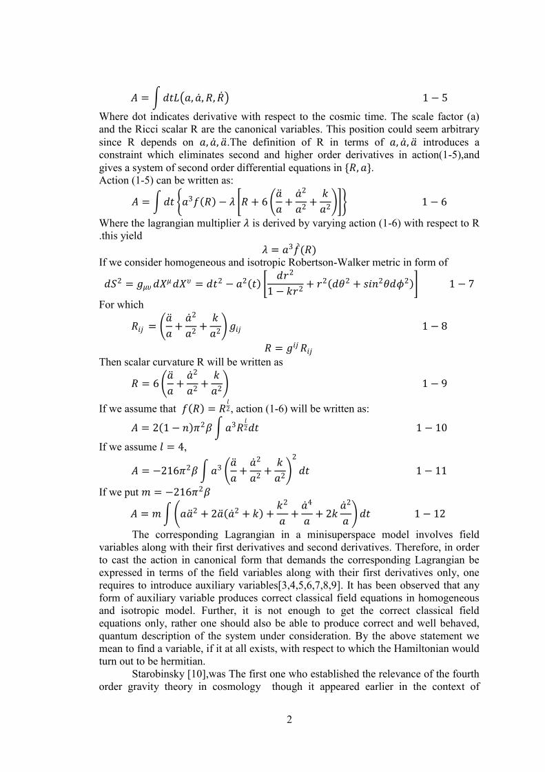
𝐴 = 𝑑𝑡𝐿 𝑎, 𝑎 , 𝑅, 𝑅 1 − 5

Where dot indicates derivative with respect to the cosmic time. The scale factor (a)

and the Ricci scalar R are the canonical variables. This position could seem arbitrary

since R depends on 𝑎, 𝑎 , 𝑎 .The definition of R in terms of 𝑎, 𝑎 , 𝑎 introduces a

constraint which eliminates second and higher order derivatives in action(1-5),and

gives a system of second order differential equations in {𝑅, 𝑎}.

Action (1-5) can be written as:

𝐴 = 𝑑𝑡 𝑎3𝑓 𝑅 − 𝜆 𝑅 + 6 𝑎

𝑎+

𝑎 2

𝑎2+

𝑘

𝑎2 1 − 6

Where the lagrangian multiplier 𝜆 is derived by varying action (1-6) with respect to R

.this yield

𝜆 = 𝑎3𝑓 (𝑅)

If we consider homogeneous and isotropic Robertson-Walker metric in form of

𝑑𝑆2 = 𝑔𝜇𝜐 𝑑𝑋𝜇𝑑𝑋𝜐 = 𝑑𝑡2 − 𝑎2 𝑡 𝑑𝑟2

1 − 𝑘𝑟2+ 𝑟2 𝑑𝜃2 + 𝑠𝑖𝑛2𝜃𝑑𝜙2 1 − 7

For which

𝑅𝑖𝑗 = 𝑎

𝑎+

𝑎 2

𝑎2+

𝑘

𝑎2 𝑔𝑖𝑗 1 − 8

𝑅 = 𝑔𝑖𝑗 𝑅𝑖𝑗

Then scalar curvature R will be written as

𝑅 = 6 𝑎

𝑎+

𝑎 2

𝑎2+

𝑘

𝑎2 1 − 9

If we assume that 𝑓 𝑅 = 𝑅𝑙2, action (1-6) will be written as:

𝐴 = 2 1 − 𝑛 𝜋2𝛽 𝑎3𝑅𝑙2𝑑𝑡 1 − 10

If we assume 𝑙 = 4,

𝐴 = −216𝜋2𝛽 𝑎3 𝑎

𝑎+

𝑎 2

𝑎2+

𝑘

𝑎2

2

𝑑𝑡 1 − 11

If we put 𝑚 = −216𝜋2𝛽

𝐴 = 𝑚 𝑎𝑎 2 + 2𝑎 𝑎 2 + 𝑘 +𝑘2

𝑎+

𝑎 4

𝑎+ 2𝑘

𝑎 2

𝑎 𝑑𝑡 1 − 12

The corresponding Lagrangian in a minisuperspace model involves field

variables along with their first derivatives and second derivatives. Therefore, in order

to cast the action in canonical form that demands the corresponding Lagrangian be

expressed in terms of the field variables along with their first derivatives only, one

requires to introduce auxiliary variables[3,4,5,6,7,8,9]. It has been observed that any

form of auxiliary variable produces correct classical field equations in homogeneous

and isotropic model. Further, it is not enough to get the correct classical field

equations only, rather one should also be able to produce correct and well behaved,

quantum description of the system under consideration. By the above statement we

mean to find a variable, if it at all exists, with respect to which the Hamiltonian would

turn out to be hermitian.

Starobinsky [10],was The first one who established the relevance of the fourth

order gravity theory in cosmology though it appeared earlier in the context of

3

quantum field theory in curved space time. Starobinsky [10] presented a solution of

the inflationary scenario without invoking phase transition in the very early Universe,

from a field equation containing only the geometric terms. However, the field

equations could not be obtained from the action principle, as the terms in the field

equations are generated from the perturbative quantum field theory. Later,

Starobinsky and Schmidt [11] have shown that the inflationary phase is an attractor in

the neighborhood of the fourth order gravity theory.

Quantum cosmology is most elusive as the role of time is not unique and one

is being unable to define the Hilbert space[12]. This is due to the fact that ‘time’ is not

an external parameter in general theory of relativity, rather it is intrinsically contained

in the theory, unlike its role in quantum mechanics or quantum field theory in flat

space time. In curved space time, different slices correspond to different choices of

time leading to inequivalent quantum theories. Likewise, the canonical quantization of

gravity is devoid of an unique time variable and hence the definition of probability of

emergence of a particular Universe out of an ensemble is ambiguous. The canonical

quantization of Einstein-Hilbert action together with some matter fields yields the

Wheeler-deWitt equation which does not contain time a priori, although it emerges

intrinsically through the scale factor of the Universe. However, if the canonical

variable is so chosen that one of the true degrees of freedom is disentangled from the

kinetic part of the canonical variables, then this kinetic part in the corresponding

quantum theory yields a quantum mechanical flavor of time. This is possible only if

the Einstein-Hilbert action is replaced by curvature squared action or modified by the

introduction of curvature squared term, in the Robertson-Walker minisuperspace

model.

Such wonderful relevance of higher order gravity theory in the context of cosmology

inspired some authors to give interpretation of the quantum cosmological

wavefunction with 𝑅2 [13] and even 𝑅3 [14] terms in the Einstein-Hilbert action.

Further the functional integral for the wavefunction of the Universe proposed by

Hartle-Hawking [15] runs into serious problem, since the wavefunction diverges

badly. There are some prescriptions [16] to avoid such divergences, though a

completely satisfactory result has not yet been obtained. However, to get a convergent

functional integral,Horowitz [9] proposed an action in the form

𝑆 = 𝑑4𝑋 𝑔 𝐴𝐶𝑖𝑗𝑘𝑙2 + 𝐵 𝑅 − 4𝜆 2 1 − 13

Where 𝐶𝑖𝑗𝑘𝑙2 is the Weyl tensor, R is the Ricci scalar, 𝜆 is the cosmological constant

and A,B are the coupling constants.

The action (1-13 ) reduces to the Einstein-Hilbert action at the weak energy limit. To

obtain a workable and simplified form of the field equations, one may consider a

spatially homogeneous and isotropic minisuperspace background, for which the Weyl

tensor trivially vanishes. A.K.Sanyal and B.Modak [3], considered the action like (1-

11) retaining only the curvature squared term. The field equations for such an action

can be obtained by the standard variation principle.

In the variational principle, the total derivative terms in the action are extracted and

one gets a surface integral which is assumed to vanish at the boundary or the action is

chosen in such a way that those surface integral terms have no contribution. However,

for canonical quantization this principle is not of much help and one has to express

the action in the canonical form, which is achieved only through the introduction of

the auxiliary variable. Auxiliary variable can be chosen in an adhoc manner, and

4

different choice of such variable would lead to different description of quantum

dynamics, keeping the classical field equations unchanged. In view of this

Ostrogradski [7] in one hand and Boulware etal [6] on the other, have made definite

prescriptions to choose such variables. Ostrogradski’s prescription [7] was followed

by Schmidt [17].

in Boulware etal’s [6] prescription the auxiliary variable should be chosen by taking

the first derivative of the action with respect to the highest derivative of the field

variable present in the action.

Hawking and Luttrell [18] utilized Boulware etal’s [6] technique to identify the new

variable and showed that the Einstein-Hilbert action along with a curvature squared

term reduces to the Einstein-Hilbert action coupled to a massive scalar field, assuming

the conformal factor. Horowitz on the other hand, showed that the canonical

quantization of the curvature squared action yields an equation which is similar to the

Schrodinger equation[9]. Pollock [19] also used the same technique to the induced

theory of gravity and obtained the same type of result as that obtained by Horowitz

[9], in the sense that the corresponding Wheeler-de Witt equation looks similar to the

Schrodinger equation.

The striking feature of Boulware etal’s [6] prescription is that it can even be applied

in situations where introduction of the auxiliary variable is not at all required, e.g. in

the induced theory of gravity, vacuum Einstein-Hilbert action etc.

The classical field equations remain unchanged with or without the introduction of

the auxiliary variables.

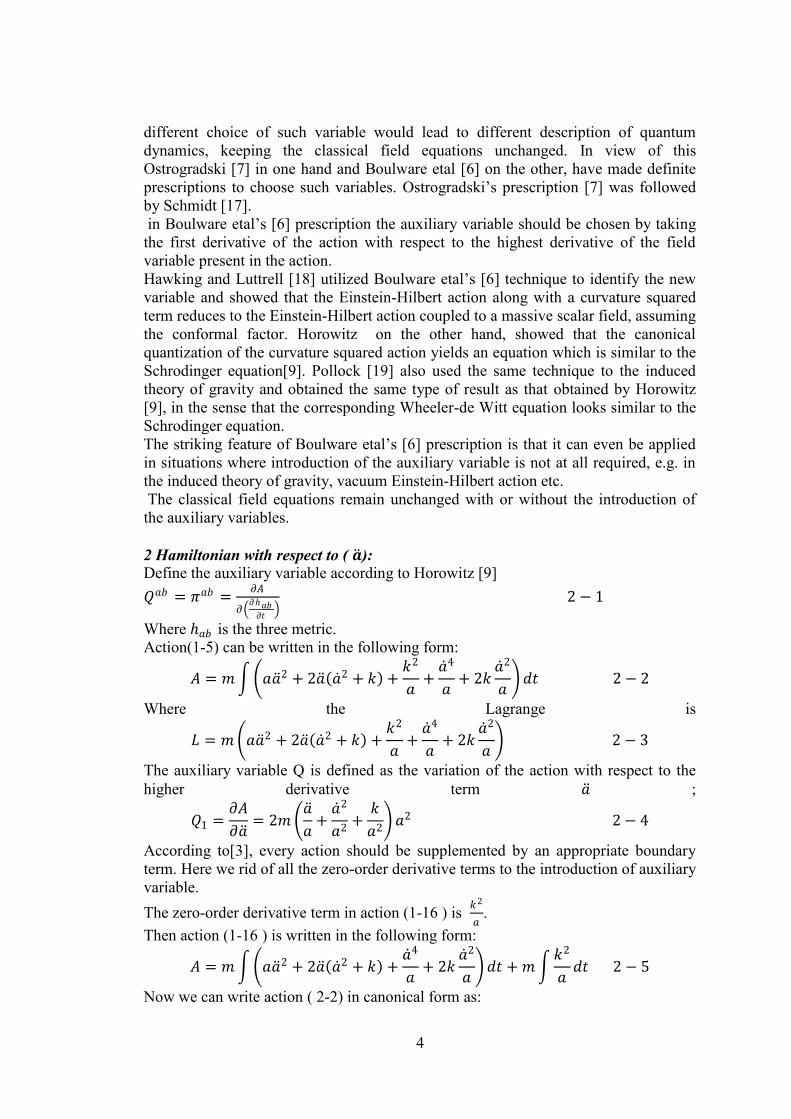
2 Hamiltonian with respect to ( 𝒂 ): Define the auxiliary variable according to Horowitz [9]

𝑄𝑎𝑏 = 𝜋𝑎𝑏 =𝜕𝐴

𝜕 𝜕𝑕𝑎𝑏

𝜕𝑡

2 − 1

Where 𝑕𝑎𝑏 is the three metric.

Action(1-5) can be written in the following form:

𝐴 = 𝑚 𝑎𝑎 2 + 2𝑎 𝑎 2 + 𝑘 +𝑘2

𝑎+

𝑎 4

𝑎+ 2𝑘

𝑎 2

𝑎 𝑑𝑡 2 − 2

Where the Lagrange is

𝐿 = 𝑚 𝑎𝑎 2 + 2𝑎 𝑎 2 + 𝑘 +𝑘2

𝑎+

𝑎 4

𝑎+ 2𝑘

𝑎 2

𝑎 2 − 3

The auxiliary variable Q is defined as the variation of the action with respect to the

higher derivative term 𝑎 ;

𝑄1 =𝜕𝐴

𝜕𝑎 = 2𝑚

𝑎

𝑎+

𝑎 2

𝑎2+

𝑘

𝑎2 𝑎2 2 − 4

According to[3], every action should be supplemented by an appropriate boundary

term. Here we rid of all the zero-order derivative terms to the introduction of auxiliary

variable.

The zero-order derivative term in action (1-16 ) is 𝑘2

𝑎.

Then action (1-16 ) is written in the following form:

𝐴 = 𝑚 𝑎𝑎 2 + 2𝑎 𝑎 2 + 𝑘 +𝑎 4

𝑎+ 2𝑘

𝑎 2

𝑎 𝑑𝑡 + 𝑚

𝑘2

𝑎𝑑𝑡

2 − 5

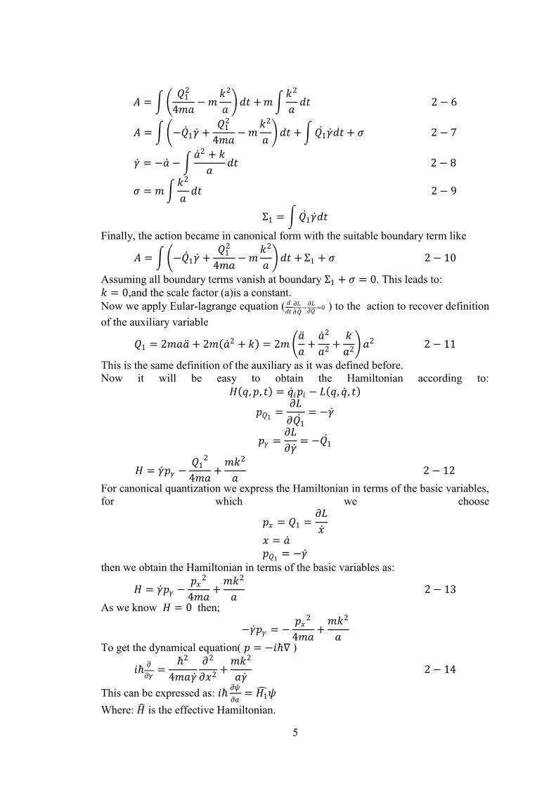
Now we can write action ( 2-2) in canonical form as:

5

𝐴 = 𝑄1

2

4𝑚𝑎− 𝑚

𝑘2

𝑎 𝑑𝑡 + 𝑚

𝑘2

𝑎𝑑𝑡 2 − 6

𝐴 = −𝑄 1𝛾 +

𝑄12

4𝑚𝑎− 𝑚

𝑘2

𝑎 𝑑𝑡 + 𝑄1

𝛾 𝑑𝑡 + 𝜍 2 − 7

𝛾 = −𝑎 − 𝑎 2 + 𝑘

𝑎𝑑𝑡 2 − 8

𝜍 = 𝑚 𝑘2

𝑎𝑑𝑡 2 − 9

Σ1 = 𝑄1 𝛾 𝑑𝑡

Finally, the action became in canonical form with the suitable boundary term like

𝐴 = −𝑄 1𝛾 +

𝑄12

4𝑚𝑎− 𝑚

𝑘2

𝑎 𝑑𝑡 + Σ1 + 𝜍 2 − 10

Assuming all boundary terms vanish at boundary Σ1 + 𝜍 = 0. This leads to:

𝑘 = 0,and the scale factor (a)is a constant.

Now we apply Eular-lagrange equation ( 𝑑

𝑑𝑡𝜕𝐿

𝜕𝑄 −𝜕𝐿𝜕𝑄

=0 ) to the action to recover definition

of the auxiliary variable

𝑄1 = 2𝑚𝑎𝑎 + 2𝑚 𝑎 2 + 𝑘 = 2𝑚 𝑎

𝑎+

𝑎 2

𝑎2+

𝑘

𝑎2 𝑎2 2 − 11

This is the same definition of the auxiliary as it was defined before.

Now it will be easy to obtain the Hamiltonian according to:

𝐻 𝑞, 𝑝, 𝑡 = 𝑞 𝑖𝑝𝑖 − 𝐿 𝑞, 𝑞 , 𝑡

𝑝𝑄1=

𝜕𝐿

𝜕𝑄1

= −𝛾

𝑝𝛾 =𝜕𝐿

𝜕𝛾 = −𝑄1

𝐻 = 𝛾 𝑝𝛾 −𝑄1

2

4𝑚𝑎+

𝑚𝑘2

𝑎 2 − 12

For canonical quantization we express the Hamiltonian in terms of the basic variables,

for which we choose

𝑝𝑥 = 𝑄1 =𝜕𝐿

𝑥

𝑥 = 𝑎 𝑝𝑄1

= −𝛾 then we obtain the Hamiltonian in terms of the basic variables as:

𝐻 = 𝛾 𝑝𝛾 −𝑝𝑥

2

4𝑚𝑎+

𝑚𝑘2

𝑎 2 − 13

As we know 𝐻 = 0 then;

−𝛾 𝑝𝛾 = −𝑝𝑥

2

4𝑚𝑎+

𝑚𝑘2

𝑎

To get the dynamical equation( 𝑝 = −𝑖ℏ∇ )

𝑖ℏ𝜕

𝜕𝛾=

ℏ2

4𝑚𝑎𝛾

𝜕2

𝜕𝑥2+

𝑚𝑘2

𝑎𝛾 2 − 14

This can be expressed as: 𝑖ℏ𝜕𝜓

𝜕𝑎= 𝐻1

𝜓

Where: 𝐻 is the effective Hamiltonian.

6

𝐻1 =

ℏ2

4𝑚𝑎𝛾

𝜕2

𝜕𝑥2+ 𝑉𝑒1 2 − 15

𝑉𝑒1 =𝑚𝑘2

𝑎𝛾 2 − 16

Represents the effective potential.

Assuming perfect fluid, which obey the equation of state p = ωρ now we can solve for 𝜌 𝑎𝑛𝑑 𝜌 in equation (3-9) and with aid of equation 𝑎

𝑎+ 2 𝑎

𝑎

2+ 2 𝑘

𝑎2 = 4𝜋𝐺 𝜌 − 𝑝 .

If the potential (2-16) remains constant with respect to time (t).we found the relation

of energy density and the scale factor , 𝜕

𝜕𝑡 𝑚𝑘2

𝑎𝛾 = 0

𝑎 𝛾 + 𝑎𝛾 = 0

𝑎 2 + 𝑎 𝑎 2 + 𝑘

𝑎𝑑𝑡 + 𝑎𝑎 + 𝑎 2 + 𝑘 = 0

Add k and divide by 𝑎2, after all we find:

2𝑎 2

𝑎2+

2𝑘

𝑎2+

𝑎

𝑎= −

𝑎

𝑎2

𝑎 2 + 𝑘

𝑎𝑑𝑡 +

𝑘

𝑎2 2 − 17

Now we can substitute equation 2 − 17 into 𝑎

𝑎+ 2 𝑎

𝑎

2+ 2 𝑘

𝑎2 = 4𝜋𝐺 𝜌 − 𝑝

4𝜋𝐺𝜌 1 − 𝜔 = −𝑎

𝑎2

𝑎 2 + 𝑘

𝑎𝑑𝑡 +

𝑘

𝑎2 2 − 18

𝜌 =𝜕𝜌

𝜕𝑡

4𝜋𝐺𝜌 1 − 𝜔 = −𝑎 2

𝑎3 𝑎 +

𝑎𝑎

𝑎 2− 2

𝑎 2 + 𝑘

𝑎𝑑𝑡 +

3𝑘

𝑎 2 − 19

𝜌

𝜌= −

𝑎

𝑎 𝑎 + 𝑎𝑎

𝑎 2− 2

𝑎 2+𝑘

𝑎𝑑𝑡 + 3𝑘

𝑎

− 𝑎 2+𝑘

𝑎𝑑𝑡 +

𝑘

𝑎

2 − 20

𝜔1 =1

3 𝑎 + 𝑎𝑎

𝑎 2− 2

𝑎 2+𝑘

𝑎𝑑𝑡 + 3𝑘

𝑎

− 𝑎 2+𝑘

𝑎𝑑𝑡 +

𝑘

𝑎

− 1 2 − 21

we consider two cases as:

1. 𝑎 → ∞; 𝑎 ≪ 1; 𝑘 ≠ 0 ,

This implies that 𝜌

𝜌~ − 3

𝑎

𝑎 2 − 22

or

𝜌 ∝ 𝑎−3 2 − 23

𝑝~0 2 − 24 with

𝜔1~0 2 − 25 This represent matter dominated universe, this means that our model described matter

era at large radius and slow expansion rate, also we found that the density is

decreasing with increasing of the radius in conformity with GR and experiments.

2. 𝑎 → 0; 𝑎 → ∞; 𝑘 ≠ 0

7

𝜌

𝜌~ − 2

𝑎

𝑎 2 − 26

where

𝜔1~ −1

3 2 − 27

which is requires negative pressure

𝑝~ −1

3𝜌 2 − 28

This result represents early universe ,which predict inflation.

3. Hamiltonian with respect to ( 𝒂 𝟐):

Now according to Boulware’s prescription[6], Hamiltonian formulation of an

action containing higher order curvature invariant term requires introduction of

auxiliary variable,

𝑄𝑎𝑏 = 𝜋𝑎𝑏 =𝜕𝐴

𝜕 𝜕𝑘𝑎𝑏

𝜕𝑡

And the extrinsic curvature 𝑘𝑎𝑏 is:

𝑘11 = 𝑘22 = 𝑘33 = −𝑎𝑎 3 − 1

The action of 𝑅2 can be written as:

𝐴 = 𝑚 𝑎𝑎 2 + 2𝑎 𝑎 2 + 𝑘 +𝑘2

𝑎+

𝑎 4

𝑎+ 2𝑘

𝑎 2

𝑎 𝑑𝑡 3 − 2

If we get rid the zero-order derivative 𝑘2

𝑎 to auxiliary variable [4],

𝐴 = 𝑚 𝑎𝑎 2 + 2𝑎 𝑎 2 + 𝑘 +𝑎 4

𝑎+ 2𝑘

𝑎 2

𝑎 𝑑𝑡 + 𝑚

𝑘2

𝑎𝑑𝑡 3 − 3

𝐴 = 𝑚 𝑎𝑎 2 + 2𝑎 𝑎 2 + 𝑘 +𝑎 4

𝑎+ 2𝑘

𝑎 2

𝑎 𝑑𝑡 + 𝜍 3 − 4

Now we supplement the action with boundary term

𝜍 = 𝑚 𝑘2

𝑎𝑑𝑡

This action can be written in the following canonical form, with

𝑄2 =𝜕𝐴

𝑎 2= 2𝑚

𝑎

𝑎+

𝑎 2

𝑎2+

𝑘

𝑎2 𝑎 3 − 5

𝐴 = −𝑄2 𝛼 +

𝑎𝑄22

4𝑚− 𝑚

𝑘2

𝑎 𝑑𝑡 + Σ2 + 𝜍 3 − 6

Σ2 = 𝑄2 𝛼

𝛼 = −𝑎𝑎 − (𝑘)𝑑𝑡 3 − 7

Assuming all boundary terms vanishing at boundary Σ2 + 𝜍 = 0 . This leads to the

same result as before:

𝑘 = 0,and the scale factor (a)is a constant.

As before we recovered the definition of the auxiliary variable by applying Eular-

lagrange.

8

For canonical quantization, we express the Hamiltonian in terms of the basic

variables, for which we choose:

𝑥 = 𝑎 2𝑑𝑡

𝑥 = 𝑎 2 and

𝑄2 = 𝑝𝑥

Now we obtain the Hamiltonian(𝐻 = 0) as:

−𝛼 𝑝𝛼 = −𝑎𝑄2

2

4𝑚+

𝑚𝑘2

𝑎 3 − 8

We express the dynamical equation as:

𝑖ℏ𝜕

𝜕𝛼=

𝑎ℏ2

4𝑚𝛼

𝜕2

𝜕𝑥 2+

𝑚𝑘2

𝑎𝛼 3 − 9

𝐻2 =

𝑎ℏ2

4𝑚𝛼

𝜕2

𝜕𝑥 2+ 𝑉𝑒2 3 − 10

where:

𝑉𝑒2 =𝑚𝑘2

𝑎𝛼 3 − 11

4𝜋𝐺𝜌 1 − 𝜔 = − 𝑎 2

𝑎4 𝑎 𝑎

𝑎 2− 3 𝑘𝑑𝑡 + 3𝑘

𝑎

𝑎 3 − 12

4𝜋𝐺𝜌 1 − 𝜔 = 𝑎

𝑎3 − 𝑘𝑑𝑡 +𝑘𝑎

𝑎 3 − 13

𝜌

𝜌= −

𝑎

𝑎 𝑎 𝑎

𝑎 2−3 𝑘𝑑𝑡 +3𝑘𝑎

𝑎

− 𝑘𝑑𝑡 +𝑘𝑎𝑎

3 − 14

𝜔2 =1

3

𝑎 𝑎

𝑎 2− 3 𝑘𝑑𝑡 + 3𝑘𝑎

𝑎

− 𝑘𝑑𝑡 +𝑘𝑎𝑎

− 1 3 − 15

According to relevant treatment of the potential, also, there are tow cases, but they are

equivalent :

1. 𝑎 → ∞; 𝑎 ≪ 1; 𝑘 ≠ 0 𝜌

𝜌~ − 3

𝑎

𝑎

this implies that

𝜔2~0 3 − 16 and

𝑝~0 𝜌 ∝ 𝑎−3

2. 𝑎 → 0; 𝑎 → ∞; 𝑘 ≠ 0 𝜌

𝜌~ − 3

𝑎

𝑎

this implies that

𝜔2~0 3 − 17 and

𝑝~0

𝜌 ∝ 𝑎−3

9

4. Comparison with A.K Sanyal work:

A.K Sanyal (according to Boulware`s prescription) choose a variable 𝑧 =𝑎2

2 then he

found the definition of the auxiliary variable Q as:

𝑄 =𝜕𝐴

𝜕𝑧 = 144𝜋2𝛽

𝑎

𝑎+

𝑎 2

𝑎2+

𝑘

𝑎2 𝑎

Then Sanyal suggestion is to get rid of all the total derivative terms prior to the

introduction of auxiliary variable. After doing this, he found the boundary term that

supplements the action is different from that one which supplements the action in

references [3,4,5] when he followed Horowitz[9].A particular action must be

supplemented by the same boundary term, independent of the choice of variable.

we found the same boundary terms in this work according to both Horowitz and

Boulware`s prescription, 𝜍 = 𝑚 𝑘2

𝑎𝑑𝑡

At boundaries we found 𝑘 = 0,and the scale factor (a)is a constant.

5. Acceleration and deceleration scenario:

In this model we did not include matter term in action (1-12),so, this model

represents curvature effects in all universal parameters, which will be added to that

parameters which was obtained from matter lagrangian.

The total effective Hamiltonian of 𝑅2 in our minisuperspace model is :

𝐻 = 𝐻 1 + 𝐻 2 =ℏ2

4𝑚𝑎 𝛾

𝜕2

𝜕𝑥2 +𝑎ℏ2

4𝑚𝛼

𝜕2

𝜕𝑥 2+ 𝑉 5 − 1

𝑉 = 𝑉𝑒1 + 𝑉𝑒2 =𝑚𝑘2

𝑎

1

𝛾 +

1

𝛼 5 − 2

The wave function is:

𝜓 = 𝜓1 + 𝜓2 = C1e2imkx

ℏ +C2e-2imkx

ℏ + 𝐷1𝑒2𝑖𝑘𝑚 𝑥

𝑎ℏ + 𝐷2𝑒−2𝑖𝑘𝑚 𝑥

𝑎ℏ 5 − 3

𝜔 = 𝜔1 + 𝜔2

𝜔 =𝑎 + 𝑎𝑎

𝑎 2− 2

𝑎 2+𝑘

𝑎𝑑𝑡 + 3𝑘

𝑎

−3 𝑎 2+𝑘

𝑎𝑑𝑡 + 3

𝑘

𝑎

+

𝑎 𝑎

3𝑎 2− 1 𝑘𝑑𝑡 + 𝑘𝑎

𝑎

− 𝑘 𝑑𝑡 + 𝑘𝑎

𝑎

− 2 5 − 4𝑎

𝜔 =𝑎 − 𝑞 + 2 𝐵 + 3

𝑘

𝑎

3𝑘

𝑎 − 3𝐵

+

𝑞

3+ 1 𝑡 − 𝐻−1

𝑡 − 𝐻−1− 2 5 − 4𝑏

Where 𝑞 = −𝑎𝑎

𝑎 2 ,the deceleration parameter, H is Hubble parameter 𝐻 =

𝑎

𝑎 ,𝐵 =

𝑎 2+𝑘

𝑎𝑑𝑡

There are two approaches, first of them represents the early universe:

1. 𝑎 → 0;

at this early time we found that, 𝜔, is dominated by the term: 𝑎 − 2 𝑎 2

𝑎𝑑𝑡

,to study how this term leads to acceleration universe, write friedmann

equation: 𝑎

𝑎= −

4𝜋𝐺

3𝜌 1 + 3𝜔

If 𝑎 ≪ 𝑎 2

𝑎𝑑𝑡 ,this case happen when we assume that the universe has phase

transition, which change 𝑎 from zero to infinity. we can rewrite the integral;

10

𝑎 2

𝑎𝑑𝑡 =

𝑎

𝑎𝑑𝑎

now we find the upper critical value of 𝜔:

𝜔 → −1

3 , and, 𝑎 → 0 .this means that, curvature did not involve in universe

revolution.

If 𝑎 is less than but comparable with 𝑎 2

𝑎𝑑𝑡 , we find:

𝜔 < −1

3 ,and, 𝑎 > 0. this implies negative pressure,𝑝 < 0 ,and 𝜌 > 𝑎−2

The negative pressure leads to inflation [20].

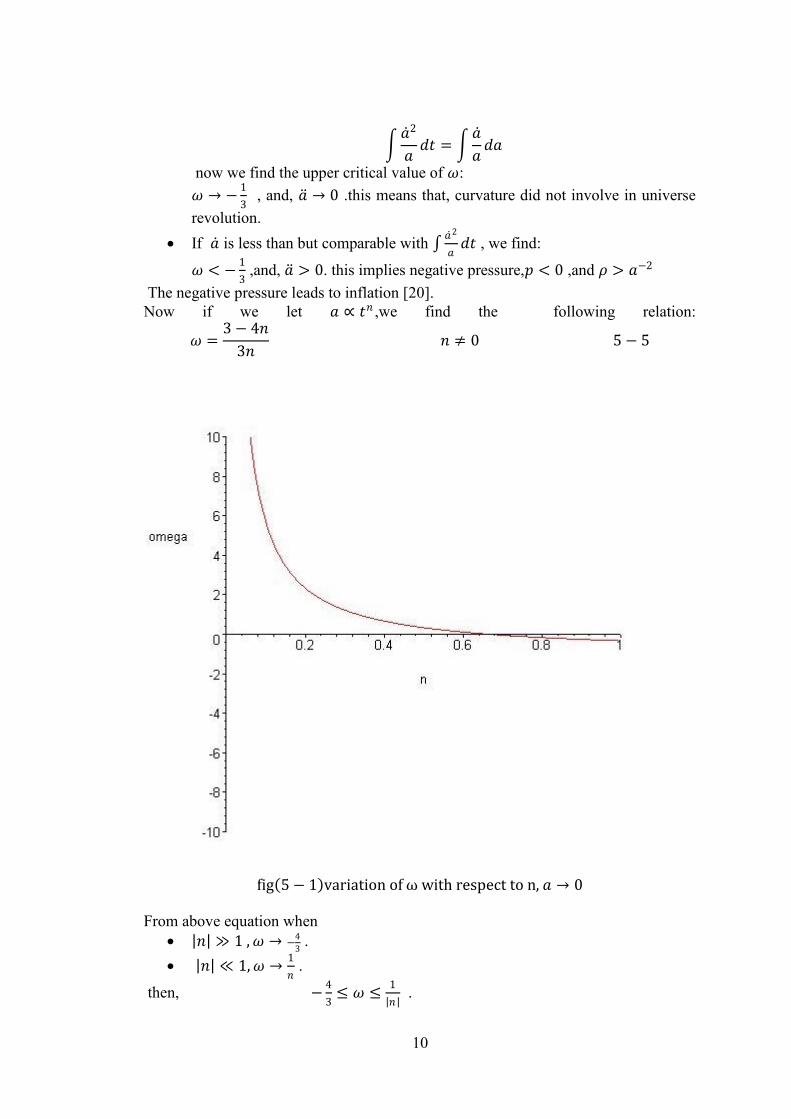
Now if we let 𝑎 ∝ 𝑡𝑛 ,we find the following relation:

𝜔 =3 − 4𝑛

3𝑛 𝑛 ≠ 0 5 − 5

fig 5 − 1 variation of ω with respect to n, 𝑎 → 0

From above equation when

𝑛 ≫ 1 , 𝜔 → −4

3 .

𝑛 ≪ 1, 𝜔 →1

𝑛 .

then, −4

3≤ 𝜔 ≤

1

𝑛 .

11

2. Second approach :𝑎 → ∞; 𝑎 ≪ 1;

𝑎 𝑎

𝑎 2≈ 0 ,this yields one value of 𝜔, where 𝜔 = 0 , and, 𝑎 < 0 ,𝜌 ∝ 𝑎−3 ,𝑝 =

0,this represents matter(relativistic particles) ,

If we turn back to action (1-6), adding matter lagrangian, means, adding a pressure

term [ 21].So, according to second approach the universe will contract very fast. May

be back to the beginning and, pre-big bang (oscillating).

6. Cosmological constant:

The boundary terms in equation (2-10) and (3-6) represent the cosmological constant.

Λ1 = 𝑄1 𝛾 + 𝑚

𝑘2

𝑎 6 − 1𝑎

Λ1 = 𝑚𝑘2

𝑎− 2𝑚 𝑎 +

𝑎 2 + 𝑘

𝑎𝑑𝑡 3𝑎 𝑎 + 𝑎𝑎 6 − 1𝑏

𝑄1 = 2𝑚 3𝑎 𝑎 + 𝑎𝑎

If the cosmological constant equal zero:

Λ1 = 0

𝑄1 𝛾 + 𝑚

𝑘2

𝑎= 0

For simplicity we let

𝑘 = 0 In this case

−𝑎 − 𝑎 2

𝑎𝑑𝑡 3𝑎 𝑎 + 𝑎𝑎 = 0 6 − 2

Solving equation (6-2)

3𝑎 𝑎 + 𝑎𝑎 = 0 6 − 3

𝑎 + 𝑎 2

𝑎𝑑𝑡 = 0 6 − 4

integrate equation (6-3) :

𝑎𝑎 + 𝑎 2 = 𝐶

𝑎𝑑2𝑎

𝑑𝑡2+

𝑑𝑎

𝑑𝑡

2

+ 𝐶 = 0 6 − 5

Differentiate equation (6-4):

𝑑

𝑑𝑡 𝑎 +

𝑎 2

𝑎𝑑𝑡 = 0

𝑎𝑎 + 𝑎 2 = 0

𝑎𝑑2𝑎

𝑑𝑡2+

𝑑𝑎

𝑑𝑡

2

= 0 6 − 6

If the integration constant 𝐶 = 0,equation (6-5) construe to equation (6-6).

Solving equation (6-6),if 𝑎 ∝ 𝑡𝑛or 𝑎 = 𝐴𝑡𝑛 ,A is a constant.

We find that:

𝑡2𝑛−2 𝑛 − 1 + 𝑛 = 0

𝑛 =1

2

By substituting in equation( 4.3-1b) that 𝑎 = 𝐴𝑡𝑛 we find:

𝑎 2+𝑘

𝑎𝑑𝑡 =

𝐴𝑛2𝑡𝑛−1

𝑛−1−

𝑘𝑡1−𝑛

𝐴 𝑛−1

12

Λ1 =𝑚𝑘2

𝐴𝑡𝑛 − 2𝑚 𝐴𝑛𝑡𝑛−1 −𝑘𝑡1−𝑛

𝐴 𝑛−1 +

𝐴𝑛2𝑡𝑛−1

𝑛−1 3𝐴2𝑛2𝑡𝑛−1 𝑛 − 1 𝑡𝑛−2 +

𝑛𝐴2𝑡𝑛 𝑛 − 1 𝑛 − 2 𝑡𝑛−3 6 − 7 Now from equation(3.3-6)

Λ2 = 𝑄2 𝛼 + 𝑚

𝑘2

𝑎 6 − 8𝑎

Λ2 = 𝑚𝑘2

𝑎− 2𝑚 𝑎 +

2𝑎𝑎 𝑎 − 𝑎 𝑘 − 𝑎 3

𝑎2 𝑎𝑎 + 𝑘𝑑𝑡 6 − 8𝑏

Λ2 = 0

𝑘 = 0

𝑎𝑎 𝑎 +2𝑎𝑎 𝑎 − 𝑎 3

𝑎2 = 0

𝑎𝑎 = 0 6 − 9

𝑎 +2𝑎𝑎 𝑎 − 𝑎 3

𝑎2= 0 6 − 10

𝑎 +𝑎 2

𝑎= 𝐶 6 − 11

When 𝐶 = 0,equation (6-11) leads to the same differential equation as equation (6-6).

By substituting in equation(6-8b) that 𝑎 = 𝐴𝑡𝑛 we find:

Λ2 =𝑚𝑘2

𝐴𝑡𝑛− 2𝑚 𝐴𝑛 𝑛 − 1 𝑛 − 2 𝑡𝑛−3

+2𝐴3𝑛2𝑡𝑛𝑡𝑛−1 𝑛 − 1 𝑡𝑛−2 − 𝐴𝑛𝑡𝑛−1𝑘 − 𝐴3𝑛3𝑡3𝑛−3

𝐴2𝑡2𝑛 𝐴2𝑛𝑡𝑛−1𝑡𝑛

+ 𝑘𝑡 6 − 12

The total cosmological constant is

Λtot = Λ1 + Λ2

Λtot =2𝑚

𝐴 −10𝐴4𝑛4𝑡3𝑛−4 + 13𝐴4𝑛3𝑡3𝑛−4 − 2𝑘𝐴2𝑛3𝑡𝑛−2 + 10𝑘𝐴2𝑛2𝑡𝑛−2

− 4𝐴4𝑛2𝑡3𝑛−4 + 𝑛𝑘2𝑡−𝑛 − 4𝑘𝐴2𝑛𝑡𝑛−2 + 𝑘2𝑡−𝑛 6 − 13

Λ = 0 𝑤𝑕𝑒𝑛 𝑛 = 0 𝑜𝑟 1

2 𝑤𝑖𝑡𝑕 𝑘 = 0

Cosmological constant vanishes at radiation era.

Now we can calculate the density parameter

ΩΛ =Λ

3𝐻2=

Λ𝑡2

3𝑛2

ΩΛ =2𝑚𝑡2

3𝐴𝑛2 −10𝐴4𝑛4𝑡3𝑛−4 + 13𝐴4𝑛3𝑡3𝑛−4 − 2𝑘𝐴2𝑛3𝑡𝑛−2 + 10𝑘𝐴2𝑛2𝑡𝑛−2

− 4𝐴4𝑛2𝑡3𝑛−4 + 𝑛𝑘2𝑡−𝑛 − 4𝑘𝐴2𝑛𝑡𝑛−2 + 𝑘2𝑡−𝑛 6 − 14

𝜌Λ =𝑚

4𝐴𝜋𝐺 −10𝐴4𝑛4𝑡3𝑛−4 + 13𝐴4𝑛3𝑡3𝑛−4 − 2𝑘𝐴2𝑛3𝑡𝑛−2 + 10𝑘𝐴2𝑛2𝑡𝑛−2

− 4𝐴4𝑛2𝑡3𝑛−4 + 𝑛𝑘2𝑡−𝑛 − 4𝑘𝐴2𝑛𝑡𝑛−2 + 𝑘2𝑡−𝑛 6 − 15 Now if we study the behavior of Λ with respect to n ,k and t we find:

1. 𝑛 → 0,

Λn=0 =2𝑚𝑘2

𝐴 6 − 16

𝜌Λ =𝑚𝑘2

4𝜋𝐴𝐺 6 − 17

13

ΩΛ =2𝑚𝑘2

3𝐴𝑛2𝑡2 =

2𝑚𝑘2

3𝐴𝐻−2 6 − 18

From above, when 𝑛 → 0, cosmological constant and vacuum energy density, remain

constants. But the density parameter, vary with time as:

𝑡 → ∞, ΩΛ → ∞.this seems to be rejected, because Ωtot = 1.

𝑡 ≈ 𝑛, ΩΛ =2𝑚𝑘2

3𝐴 ,

𝑡 → 0, ΩΛ → 0 .

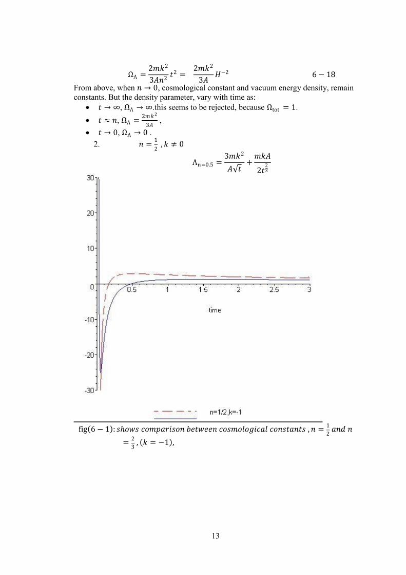
2. 𝑛 =1

2 , 𝑘 ≠ 0

Λn=0.5 =3𝑚𝑘2

𝐴 𝑡+

𝑚𝑘𝐴

2𝑡23

fig 6 − 1 : 𝑠𝑕𝑜𝑤𝑠 𝑐𝑜𝑚𝑝𝑎𝑟𝑖𝑠𝑜𝑛 𝑏𝑒𝑡𝑤𝑒𝑒𝑛 𝑐𝑜𝑠𝑚𝑜𝑙𝑜𝑔𝑖𝑐𝑎𝑙 𝑐𝑜𝑛𝑠𝑡𝑎𝑛𝑡𝑠 , 𝑛 =1

2 𝑎𝑛𝑑 𝑛

=2

3 , 𝑘 = −1 ,

14

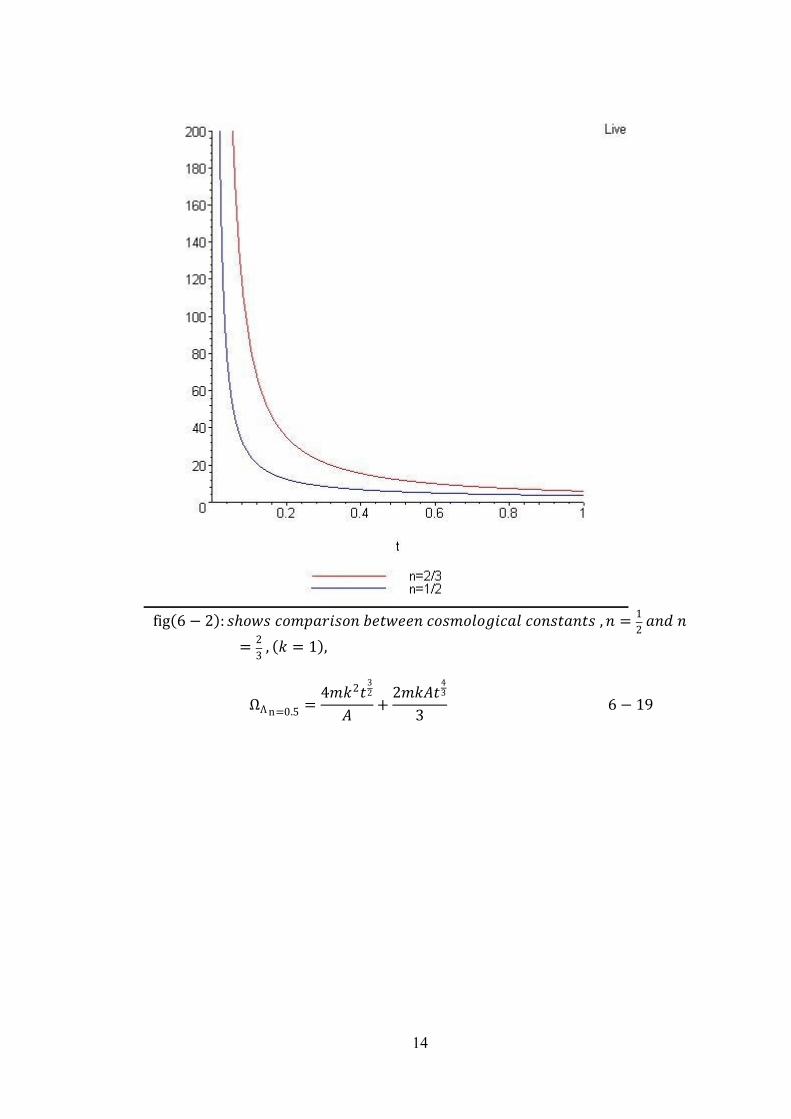
fig 6 − 2 : 𝑠𝑕𝑜𝑤𝑠 𝑐𝑜𝑚𝑝𝑎𝑟𝑖𝑠𝑜𝑛 𝑏𝑒𝑡𝑤𝑒𝑒𝑛 𝑐𝑜𝑠𝑚𝑜𝑙𝑜𝑔𝑖𝑐𝑎𝑙 𝑐𝑜𝑛𝑠𝑡𝑎𝑛𝑡𝑠 , 𝑛 =1

2 𝑎𝑛𝑑 𝑛

=2

3 , 𝑘 = 1 ,

ΩΛ n=0.5=

4𝑚𝑘2𝑡32

𝐴+

2𝑚𝑘𝐴𝑡43

3 6 − 19

15

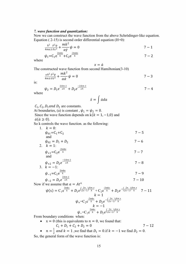
7. wave function and quantization:

Now we can construct the wave function from the above Schrödinger-like equation.

Equation ( 2-15) is second order differential equation (H=0):

ℏ2

4𝑚𝑎 𝛾

𝜕2𝜓

𝜕𝑥2 +𝑚𝑘2

𝑎𝛾 𝜓 = 0 7 − 1

𝜓1=C1e2imkx

ℏ +C2e-2imkx

ℏ 7 − 2 where

𝑥 = 𝑎 The constructed wave function from second Hamiltonian(3-10)

𝑎ℏ2

4𝑚𝛼

𝜕2𝜓

𝜕𝑥 2+

𝑚𝑘2

𝑎𝛼 𝜓 = 0 7 − 3

is:

𝜓2 = 𝐷1𝑒2𝑖𝑘𝑚 𝑥

𝑎ℏ + 𝐷2𝑒−2𝑖𝑘𝑚 𝑥

𝑎ℏ 7 − 4 where

𝑥 = 𝑎 𝑑𝑎

𝐶1, 𝐶2, 𝐷1𝑎𝑛𝑑 𝐷2 are constants.

At boundaries, (a) is constant , 𝜓1 = 𝜓2 = 0.

Since the wave function depends on k 𝑘 = 1, −1,0 and

𝑎 𝑎 ≥ 0 .

So k controls the wave function. as the following:

1. 𝑘 = 0:

𝜓01=C1+C2 7 − 5 and

𝜓02 = 𝐷1 + 𝐷2 7 − 6

2. 𝑘 = 1:

𝜓+1=C2e-2imkx

ℏ 7 − 7 and

𝜓+2 = 𝐷2𝑒−2𝑖𝑘𝑚 𝑥

𝑎ℏ 7 − 8

3. 𝑘 = −1:

𝜓−1=C1e2imkx

ℏ 7 − 9

𝜓−2 = 𝐷1𝑒2𝑖𝑘𝑚 𝑥

𝑎ℏ 7 − 10

Now if we assume that 𝑎 = 𝐴𝑡𝑛

𝜓 x = C1e2imkx

ℏ + 𝐷1𝑒

2𝑛

2𝑛−1 𝑖𝑘𝑚 x

ℏ + C2e-2imkx

ℏ + 𝐷2𝑒− 2𝑛

2𝑛−1 𝑖𝑘𝑚 x

ℏ 7 − 11

𝑘 = 1

𝜓+=C2e-2imkx

ℏ + 𝐷2𝑒−

2𝑛

2𝑛−1 𝑖𝑘𝑚 x

ℏ 𝑘 = −1

𝜓−=C1e2imkx

ℏ + 𝐷1𝑒

2𝑛

2𝑛−1 𝑖𝑘𝑚 x

ℏ From boundary conditions when:

x = 0 (this is equivalents to 𝑛 = 0, we found that:

𝐶1 + 𝐷1 + 𝐶2 + 𝐷2 = 0 7 − 12

𝑛 =1

2 𝑎𝑛𝑑 𝑘 = 1 ,we find that 𝐷1 = 0.if 𝑘 = −1 we find 𝐷2 = 0.

So, the general form of the wave function is:

16

𝜓 x = C1e2i 𝑘 mx

ℏ + C2e-2i 𝑘 mx

ℏ − C1 + C2 𝑒−

2𝑛

2𝑛−1 𝑖 𝑘 𝑚 x

ℏ 7 − 13

We can recognize that from(7 − 5,7 − 6,7 − 12) flat universe,𝑘 = 0, is equivalent to

static one 𝑎 = 𝑐𝑜𝑛𝑠𝑡𝑎𝑛𝑡 .

1. 𝑛 = 1, 𝑎 ∝ 𝑡 ,we find the second wave function phase reduced to the first one

,

𝜓 x = C1e2i 𝑘 mx

ℏ − C1e-2i 𝑘 mx

ℏ = 2𝑖 C1 sin2 𝑘 𝑚x

ℏ 7 − 14

2. As we know at radiation era 𝑎 ∝ 𝑡12 , 𝑛 =

1

2 ,then, the wave function takes the

following form:

𝜓 x =C1e2i 𝑘 mx

ℏ + C2e-2i 𝑘 mx

ℏ 7 − 15

We get from 7-14 and 7-15 𝐶1 = −𝐶2 .𝐷2 = 0

Using 7-14 to find out C1 by normalizing the wave function, 𝜓𝜓∗dx = 1

2𝑖 C1 sin2 𝑘 𝑚x

ℏ

2

dx

𝐴

0

= 1

𝐶1 = 𝑏

sin 2𝐴𝑏−2𝐴𝑏 7 − 16

Where : 𝑏 =2 𝑘 𝑚

ℏ .

According to this limit −∞ ≤𝑏

sin 2𝐴𝑏−2𝐴𝑏≤ −1 and since 𝐴 ≥ 0 , 𝐶1 is complex

number .

We can write 7-14 as:

𝜓 𝑎 = 2 𝑏

2𝐴𝑏 − sin 2𝐴𝑏 sin 𝑏𝑎 7 − 17

Also, we found that

0 ≤ 𝑛 ≤ 1 7 − 18 According to 5-5 and 7-18 , at early universe vacuum dose not dominate the universe.

So the limit of 𝜔 is reduced to:

−1

3≤ 𝜔 ≤

1

𝑛 7 − 19

We can find the probability, which we can call it density parameter Ω, to our universe,

from 7-17

𝑃 ≡ Ω =4𝑏

2𝐴𝑏 − sin 2𝐴𝑏sin2 𝑏𝑎 7 − 20𝑎

𝑃 ≡ Ω =8 𝑘 𝑚

4𝐴 𝑘 𝑚 − ℏ sin4𝐴 𝑘 𝑚

ℏ

sin2 2 𝑘 𝑚

ℏ𝑎 7 − 20𝑏

When 2𝐴𝑏 ≫ sin 2𝐴𝑏 , we find that Ω =2

𝐴sin2 𝑏𝑎 .

If we take the probability in flat and unaccelerated universe(appindixI-3),

lim𝑘=0,𝑎 =𝐴

Ω =3

𝐴 7 − 21

Now ,if we take the limit of the probability in flat and accelerated universe,

lim𝑘=0

Ω =3𝑎 2

𝐴3 7 − 22

Using Friedmann equation ,where 𝑘 = 0 we find:

17

lim𝑘=0

Ω =8𝜋𝐺𝜌𝑎2

𝐴3 7 − 23

Maximum probability, Ω = 1 , occurs when, 𝑘 ≠ 0, and:

𝑎 𝑐 =ℏ

2𝑚sin−1

4𝐴𝑚−ℏ sin4𝐴𝑚

ℏ

8𝑚 7 − 24

Where 𝑎 ∝ 𝑡𝑛 .

𝑡𝑐 = ℏ

2𝐴𝑛𝑚sin−1

4𝐴𝑚−ℏ sin4𝐴𝑚

ℏ

8𝑚

1

𝑛−1

7 − 25

𝑎𝑐 = 𝐴 ℏ

2𝐴𝑛𝑚sin−1

4𝐴𝑚−ℏ sin4𝐴𝑚

ℏ

8𝑚

𝑛

𝑛−1

7 − 26

𝐻𝑐 = 𝑛 𝑛

𝑛−1

ℏ

2𝐴𝑚sin−1

4𝐴𝑚−ℏ sin4𝐴𝑚

ℏ

8𝑚

1

1−𝑛

7 − 27

lim𝑛→0

𝑎𝑐 = 𝐴 7 − 28

lim𝑛→1

𝑎𝑐 = ∞ 7 − 29

lim𝑛→0

𝐻𝑐 =𝑎 𝑐𝐴

7 − 30

The subscript( 𝑐) refers to critical value ,which occurs at maximum probability.

From 7-20, Ω =8𝜋𝐺𝜌

3𝐻2 , we find:

𝜌 =3 𝑘 𝑚

𝜋𝐺

𝐻2

4𝐴 𝑘 𝑚 − ℏ sin4𝐴 𝑘 𝑚

ℏ

sin2 2 𝑘 𝑚𝑎

ℏ 7 − 31𝑎

Where 𝑘 ≠ 0, we find:

𝜌 =3𝑚

𝜋𝐺

𝐻2

4𝐴𝑚 − ℏ sin4𝐴𝑚

ℏ

sin2 2𝑚𝑎

ℏ 7 − 31𝑏

𝜌𝑐 =3

8𝜋𝐺

𝑛 2𝑛

𝑛−1

4𝐴𝑚 − ℏ sin4𝐴𝑚

ℏ

ℏ

2𝐴𝑚sin−1

4𝐴𝑚−ℏ sin4𝐴𝑚

ℏ

8𝑚

2

1−𝑛

4𝐴𝑚−ℏ𝑠𝑖𝑛4𝐴𝑚

ℏ 7 − 32

7-31,must satisfy the condition:

𝐴 × 𝑚 >ℏ

4 7 − 33

If we consider, that,𝑎 → 0 ; 7-31 reads:

𝜌 𝑎 →0 =12𝑚3𝑘2

𝜋ℏ2𝐺

𝐻4𝑎2

4𝐴𝑚 − ℏ sin4𝐴𝑚

ℏ

7 − 34

Now we define the continuity equation: 𝜕𝑃

𝜕𝑡+ ∇ . 𝑗 = 0 7 − 35

J current density =𝑖ℏ

2𝑚 Ψ

𝜕Ψ∗

𝜕𝑎 − Ψ∗

𝜕Ψ

𝜕𝑎 = 0 7 − 36

𝜕𝑃

𝜕𝑡=

32 𝑘2𝑚2𝑛 𝑛 − 1 𝑡 𝑛−1

4𝐴 𝑘 𝑚 − ℏ𝑠𝑖𝑛4𝐴 𝑘 𝑚

ℏ ℏ𝑡

cos2𝐴𝑛 𝑘 𝑚𝑡 𝑛−1

ℏsin

2𝐴𝑛 𝑘 𝑚𝑡 𝑛−1

ℏ = 0

Now we can solve for (t),(n).(appindixI-4);

18

𝑡 𝑛 = exp ln

±𝜋ℏ

4𝐴 𝑘 𝑛𝑚

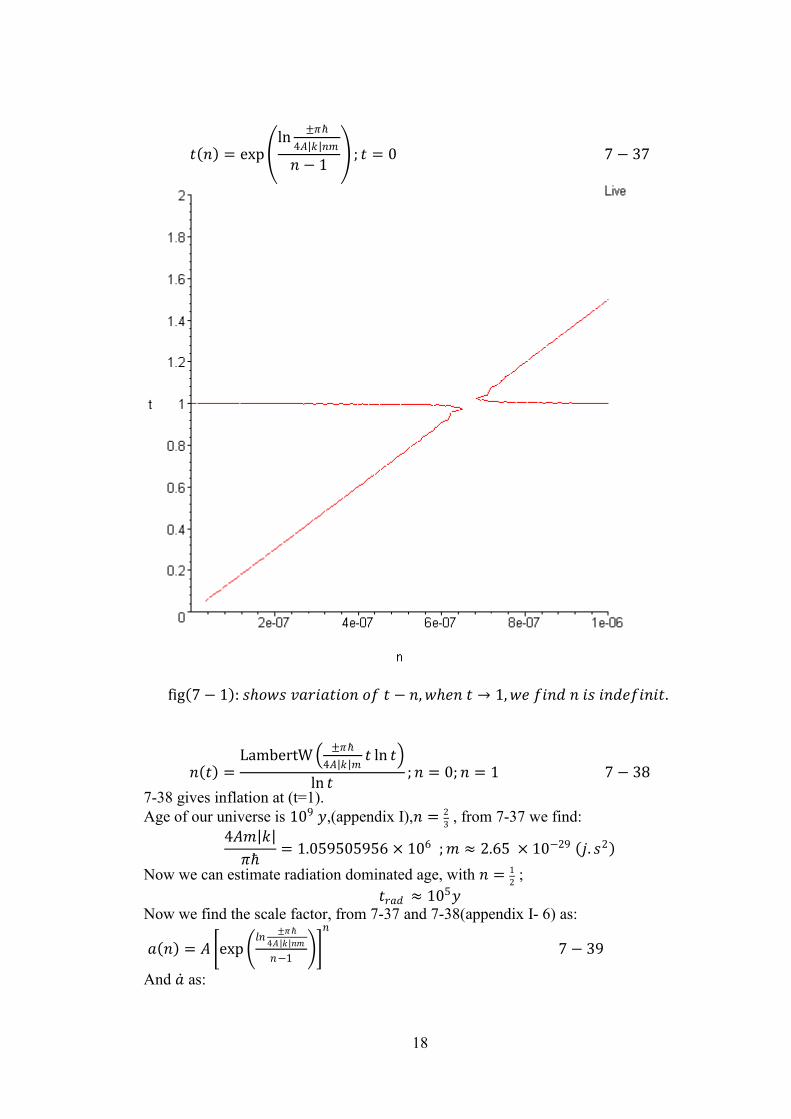
𝑛 − 1 ; 𝑡 = 0 7 − 37

fig 7 − 1 : 𝑠𝑕𝑜𝑤𝑠 𝑣𝑎𝑟𝑖𝑎𝑡𝑖𝑜𝑛 𝑜𝑓 𝑡 − 𝑛, 𝑤𝑕𝑒𝑛 𝑡 → 1, 𝑤𝑒 𝑓𝑖𝑛𝑑 𝑛 𝑖𝑠 𝑖𝑛𝑑𝑒𝑓𝑖𝑛𝑖𝑡.

𝑛 𝑡 =LambertW

±𝜋ℏ

4𝐴 𝑘 𝑚𝑡 ln 𝑡

ln 𝑡; 𝑛 = 0; 𝑛 = 1 7 − 38

7-38 gives inflation at (t=1).

Age of our universe is 109 𝑦,(appendix I),𝑛 = 2

3 , from 7-37 we find:

4𝐴𝑚 𝑘

𝜋ℏ= 1.059505956 × 106 ; 𝑚 ≈ 2.65 × 10−29 𝑗. 𝑠2

Now we can estimate radiation dominated age, with 𝑛 = 1

2 ;

𝑡𝑟𝑎𝑑 ≈ 105𝑦 Now we find the scale factor, from 7-37 and 7-38(appendix I- 6) as:

𝑎 𝑛 = 𝐴 exp 𝑙𝑛

±𝜋ℏ

4𝐴 𝑘 𝑛𝑚

𝑛−1

𝑛

7 − 39

And 𝑎 as:

19

𝑎 𝑛 = 𝐴𝑛 exp 𝑙𝑛

±𝜋ℏ

4𝐴 𝑘 𝑛𝑚

𝑛 − 1

𝑛−1

7 − 40

And acceleration is given by(appendix I- 7):

𝑎 𝑛 = 𝐴𝑛 𝑛 − 1 exp 𝑙𝑛

±𝜋ℏ

4𝐴 𝑘 𝑛𝑚

𝑛 − 1

𝑛−2

7 − 41

𝐻 𝑛 = 𝑛 exp 𝑙𝑛

±𝜋ℏ

4𝐴 𝑘 𝑛𝑚

𝑛 − 1

−1

7 − 42

appendix I-8 to calculate mass density and Hubble constant .

From 7-24 and( appendix I-6) ,we can estimate the value of

sin−1 4𝐴𝑚 −ℏ sin

4𝐴𝑚ℏ

8𝑚= 𝜋

2 ; 𝑜𝑟 4𝐴𝑚−ℏ𝑠𝑖𝑛

4𝐴𝑚

ℏ

8𝑚= 1 7 − 43

8. Complex solution:

Now we solved 7-37 in context of the term 𝜋ℏ

4𝐴 𝑘 𝑚, according to (appendix I-

4) we find:

𝜋ℏ

4𝐴 𝑘 𝑚= −4.4 × 10−7 ± 7.6 × 10−7𝑖 8 − 1

If we assume that, the constant ,A, is a complex, using 8-1,we find:

𝐴 = 1 + 1.7321𝑖 𝜋, 𝐴∗ = (1 − 1.7321𝑖 )𝜋 8 − 2

4𝐴𝑚 − ℏ 𝑠𝑖𝑛4𝐴𝑚

ℏ

8𝑚= −.1276 + .2265𝑖 8 − 3

By substituting 8-1 and 8-2 in 7-39( appendix I-9) ,7-40( appendix I-10),7-41(

appendix I-11)and 7-42( appendix I-12).

From appendix I-11, our today universe acceleration (𝑛 = 2

3) can be assigned to the

imaginary part of 𝑎 . Also we can find the density, by substituting 8-3 in 7-31, (

appendix I-13).

If we treat the cosmic back ground radiation as black body radiation, and

according to Stefan`s law of radiation:

𝜍𝑇4 ∝ 𝐸

𝑇 = 4

3𝜍𝜋𝐴3

𝑎0

𝑎𝑟

3

𝑓𝜌𝑟 1

1 + 𝑧

2

4

8 − 4

Where 𝑓 is the ratio of redshifted radiation density.

0 ≤ 𝑓 ≤ 1

8-3 represents maximum(limit) CBR temperature when 𝑓 = 1

If we substitute the values from which we found ,from our work, we get:

𝑓 = 1

𝑇 = 5.3 − 3.1𝑖 𝑘

When 𝑓 = 0.07

𝑇 = 2.726 − 1.58𝑖 𝑘

20

Now if we choose the scale factor with variable A as:

𝑎 = 𝐴𝑛𝑡𝑛 8 − 5

Now we can rewrite our equations as:

𝑃 ≡ Ω =8 𝑘 𝑚

4𝐴𝑛 𝑘 𝑚 − ℏ sin4𝐴𝑛 𝑘 𝑚

ℏ

sin2 2 𝑘 𝑚

ℏ𝑎 8 − 6

𝜌 =3 𝑘 𝑚

𝜋𝐺

𝐻2

4𝐴𝑛 𝑘 𝑚−ℏ sin4𝐴𝑛 𝑘 𝑚

ℏ sin2

2 𝑘 𝑚𝑎

ℏ 8 − 7

𝑡 𝑛 = exp ln

±𝜋ℏ

4 𝑘 𝑛𝑚− 𝑛 ln 𝐴

𝑛 − 1 ; 𝑡 = 0 8 − 9

𝑛 𝑡 =LambertW

±𝜋ℏ

4𝐴 𝑘 𝑚𝑡 ln 𝐴𝑡

ln 𝐴𝑡; 𝑛 = 0; 𝑛 = 1 8 − 10

𝑇 = (1.89654434 − 1.8965443381𝑖) 𝐾

With absolute value,𝑇 = 2.682118726 𝐾

When the age of universe is:

𝑡 = 13.75 𝐺𝑦 Which is agree with recent observations.

9. Results and Discussion:

We have seen that the canonical quantization formalism adopted in this work

has brought interesting results. We have solved the Wheeler-De Witt equation and

obtained the wave function of the universe. The wave function vanishes when

𝑎 → 0 . We found that density parameter is related to probability. Moreover, we have

found that the scale factor is imaginary. From Stefan's law we have found the cosmic

microwave background radiation (CMBR) temperature.

Considering the model of 𝑎 it is important to note that in case of 𝑎 → ∞ , 𝑎 ≪ 1 , i.e.

when the universe radius is large, the expansion rate is slow, equation (2-26) which is

the expression for the density reduces to that of GR, the density of universe decreases

with time as radius increases in conformity with observations. It also indicates that the

pressure, P, vanishes, equation 2.28, which also agrees with GR and observations at

matter era.

Thus, this case represents matter era in GR. When the radius is assumed to be very

small with high expansion rate i.e. 𝑎 → 0 , 𝑎 → ∞, as happens at early universe, the

pressure becomes negative ,equation 2.32. This also agrees with inflation assumption.

The model for 𝑎 2 gives also some interesting results, it shows that 𝜌 ∝ 𝑎−3 and 𝑝 = 0

which can suitably describing matter era only.

The boundary term 𝜍 for this model coincides with the one emerging from that of the

model 𝑎 , as shown by equation 2.9.

21

The two cosmological constant Λ1 and Λ2 for the model 𝑎 and 𝑎 2 show also some

interesting properties. They both vanishes at radiation era, when 𝑎 = 𝐴𝑡1

2 .

As seen in equations (6-2), (6-7), (6.9) and (6-13), equation (6-19) shows that the total

cosmological constant decreases as time increases. This agrees with inflation models

at the early universe.

The wavefunction 𝜓1 and 𝜓2 of the universe for both models are also obtained in

section [7]. The complex form of the solution in (7-13) shows the existance of

quantum effects. The complex nature of cosmic scale factor shown in (8-2) confirms

the existance of quantum effects. The CBR temperature is found to agree with the

experimental range , equation 8-5.

APPENDIX

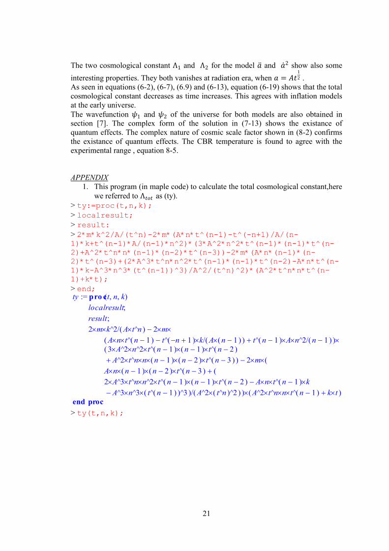
1. This program (in maple code) to calculate the total cosmological constant,here

we referred to Λ𝑡𝑜𝑡 as (ty).

> ty:=proc(t,n,k);

> localresult;

> result:

> 2*m*k^2/A/(t^n)-2*m*(A*n*t^(n-1)-t^(-n+1)/A/(n-

1)*k+t^(n-1)*A/(n-1)*n^2)*(3*A^2*n^2*t^(n-1)*(n-1)*t^(n-

2)+A^2*t^n*n*(n-1)*(n-2)*t^(n-3))-2*m*(A*n*(n-1)*(n-

2)*t^(n-3)+(2*A^3*t^n*n^2*t^(n-1)*(n-1)*t^(n-2)-A*n*t^(n-

1)*k-A^3*n^3*(t^(n-1))^3)/A^2/(t^n)^2)*(A^2*t^n*n*t^(n-

1)+k*t);

> end;

> ty(t,n,k);

ty , ,t n kpro c( ) :=

localresult;

result;

/( )2 m ^k 2 A ^t n 2 m

( ) A n ^t ( )n 1 /( )^t ( ) n 1 k A ( )n 1 /( )^t ( )n 1 A ^n 2 n 1

3 ^A 2 ^n 2 ^t ( )n 1 ( )n 1 ^t ( )n 2(

^A 2 ^t n n ( )n 1 ( )n 2 ^t ( )n 3 ) 2 m (

A n ( )n 1 ( )n 2 ^t ( )n 3 (

2 ^A 3 ^t n ^n 2 ^t ( )n 1 ( )n 1 ^t ( )n 2 A n ^t ( )n 1 k

^A 3 ^n 3 ^( )^t ( )n 1 3 ^A 2 ^( )^t n 2)/( ) ) ( ) ^A 2 ^t n n ^t ( )n 1 k t

end proc

22

> R0 := simplify(2*m*k^2/A/(t^n)-2*m*(A*n*t^(n-1)-t^(-n+1)/A/(n-1)*k+t^(n-1)*A/(n-1)*n^2)*(3*A^2*n^2*t^(n-

1)*(n-1)*t^(n-2)+A^2*t^n*n*(n-1)*(n-2)*t^(n-3))-

2*m*(A*n*(n-1)*(n-2)*t^(n-3)+(2*A^3*t^n*n^2*t^(n-1)*(n-

1)*t^(n-2)-A*n*t^(n-1)*k-A^3*n^3*(t^(n-

1))^3)/A^2/(t^n)^2)*(A^2*t^n*n*t^(n-1)+k*t));

> R1 := combine(R0,power);

> ty(t,0,0);

> ty(t,.5,0);

> ty(t,1/2,-1);

> R18 := simplify(2*m/A/t^(1/2)-2*m*(3/8*A/t^(5/2)+(-

3/8*A^3/t^(3/2)+1/2*A/t^(1/2))/A^2/t)*(1/2*A^2-t));

> R19 := expand(R18);

> ty(t,1/2,1);

2 m k2

A tn2 m

A n t

( )n 1 t( ) n 1

k

A ( )n 1

t( )n 1

A n2

n 1

( )3 A2 n2 t( )n 1

( )n 1 t( )n 2

A2 tn n ( )n 1 ( )n 2 t( )n 3

2 m

A n ( )n 1 ( )n 2 t( )n 3

2 A3 tn n2 t( )n 1

( )n 1 t( )n 2

A n t( )n 1

k A3 n3 ( )t( )n 1

3

A2 ( )tn2

( )A2 tn n t( )n 1

k t

R0 2 10 A4 n4 t( )3 n 4

13 A4 n3 t( )3 n 4

2 A2 n3 t( )n 2

k 10 A2 n2 t( )n 2

k ( :=

4 A4 n2 t( )3 n 4

t( )n

n k2 4 A2 n t( )n 2

k t( )n

k2 ) m A/

R1 2 10 A4 n4 t( )3 n 4

13 A4 n3 t( )3 n 4

2 A2 n3 t( )n 2

k 10 A2 n2 t( )n 2

k ( :=

4 A4 n2 t( )3 n 4

t( )n

n k2 4 A2 n t( )n 2

k t( )n

k2 ) m A/

0

0.

2 m

A t2 m

3 A

8 t( )/5 2

3 A3

8 t( )/3 2

A

2 t

A2 t

A2

2t

:= R18m ( )6 t A2

2 t( )/3 2

A

:= R19 3 m

A t

m A

2 t( )/3 2

2 m

A t2 m

3 A

8 t( )/5 2

3 A3

8 t( )/3 2

A

2 t

A2 t

A2

2t

23

> R20 := simplify(2*m/A/t^(1/2)-2*m*(3/8*A/t^(5/2)+(-3/8*A^3/t^(3/2)-1/2*A/t^(1/2))/A^2/t)*(1/2*A^2+t));

> R21 := expand(R20);

> ty(t,2/3,-1);

> R22 := simplify(2*m/A/t^(2/3)+8/27*m*(-2/3*A/t^(1/3)-3*t^(1/3)/A)*A^2/t^(5/3)-2*m*(8/27*A/t^(7/3)+(-

16/27*A^3/t+2/3*A/t^(1/3))/A^2/t^(4/3))*(2/3*A^2*t^(1/3)-

t));

> R23 := expand(R22);

> ty(t,2/3,1);

> R24 := simplify(2*m/A/t^(2/3)+8/27*m*(-2/3*A/t^(1/3)+3*t^(1/3)/A)*A^2/t^(5/3)-

2*m*(8/27*A/t^(7/3)+(-16/27*A^3/t-

2/3*A/t^(1/3))/A^2/t^(4/3))*(2/3*A^2*t^(1/3)+t));

> R25 := expand(R24);

:= R20m ( )6 t A2

2 t( )/3 2

A

:= R21 3 m

A t

m A

2 t( )/3 2

2 m

A t( )/2 3

8 m

2 A

3 t( )/1 3

3 t( )/1 3

AA2

27 t( )/5 3

2 m

8 A

27 t( )/7 3

16 A3

27 t

2 A

3 t( )/1 3

A2 t( )/4 3

2 A2 t( )/1 3

3t

:= R22 2 m ( ) 135 t

( )/5 38 A4 t

( )/1 396 A2 t

81 t( )/7 3

A

:= R23 10 m

3 A t( )/2 3

16 m A3

81 t2

64 m A

27 t( )/4 3

2 m

A t( )/2 3

8 m

2 A

3 t( )/1 3

3 t( )/1 3

AA2

27 t( )/5 3

2 m

8 A

27 t( )/7 3

16 A3

27 t

2 A

3 t( )/1 3

A2 t( )/4 3

2 A2 t( )/1 3

3t

:= R242 m ( ) 135 t

( )/5 38 A4 t

( )/1 396 A2 t

81 t( )/7 3

A

:= R25 10 m

3 A t( )/2 3

16 m A3

81 t2

64 m A

27 t( )/4 3

24

> ty(t,n,0);

> ty(t,1/2,k);

> R0 := simplify(2*m*k^2/A/t^(1/2)-2*m*(3/8*A/t^(5/2)+(-

3/8*A^3/t^(3/2)-1/2*A/t^(1/2)*k)/A^2/t)*(1/2*A^2+k*t));

> R1 := expand(R0);

> limit(R1,t=infinity);

2. This is maple code to calculate Λ , ΩΛ and ρΛ

> lmabda=m*k^2/A/(t^n)-2*m*(A*n*t^(n-1)-t^(-n+1)/A/(n-1)*k+t^(n-1)*A/(n-1)*n^2)*(3*A^2*n^2*t^(n-1)*(n-1)*t^(n-

2)+A^2*t^n*n*(n-1)*(n-2)*t^(n-3))+m*k^2/A/(t^n)-

2*m*(A*n*(n-1)*(n-2)*t^(n-3)+(2*A^3*t^n*n^2*t^(n-1)*(n-

1)*t^(n-2)-A*n*t^(n-1)*k-A^3*n^3*(t^(n-

1))^3)/A^2/(t^n)^2)*(A^2*t^n*n*t^(n-1)+k*t);

> R16 := rhs(lambda = 2*m*k^2/A/(t^n)-2*m*(A*n*t^(n-1)-t^(-n+1)/A/(n-1)*k+t^(n-1)*A/(n-1)*n^2)*(3*A^2*n^2*t^(n-

2 m

A n t

( )n 1 t( )n 1

A n2

n 1

( )3 A2 n2 t( )n 1

( )n 1 t( )n 2

A2 tn n ( )n 1 ( )n 2 t( )n 3

2 m

A n ( )n 1 ( )n 2 t( )n 3 2 A3 tn n2 t

( )n 1( )n 1 t

( )n 2A3 n3 ( )t

( )n 13

A2 ( )tn2

A2 tn

n t( )n 1

2 m k2

A t2 m

3 A

8 t( )/5 2

3 A3

8 t( )/3 2

A k

2 t

A2 t

A2

2k t

:= R0m k ( )6 k t A2

2 t( )/3 2

A

:= R1 3 m k2

A t

m k A

2 t( )/3 2

0

lmabda2 m k2

A tn2 m

A n t

( )n 1 t( ) n 1

k

A ( )n 1

t( )n 1

A n2

n 1

( )3 A2 n2 t( )n 1

( )n 1 t( )n 2

A2 tn n ( )n 1 ( )n 2 t( )n 3

2 m

A n ( )n 1 ( )n 2 t( )n 3

2 A3 tn n2 t( )n 1

( )n 1 t( )n 2

A n t( )n 1

k A3 n3 ( )t( )n 1

3

A2 ( )tn2

( )A2 tn n t( )n 1

k t

25

1)*(n-1)*t^(n-2)+A^2*t^n*n*(n-1)*(n-2)*t^(n-3))-

2*m*(A*n*(n-1)*(n-2)*t^(n-3)+(2*A^3*t^n*n^2*t^(n-1)*(n-

1)*t^(n-2)-A*n*t^(n-1)*k-A^3*n^3*(t^(n-

1))^3)/A^2/(t^n)^2)*(A^2*t^n*n*t^(n-1)+k*t));

> R17 := simplify(R16);

> R5 := expand(R17);

> R6 := collect(R5,k);

This is ΩΛ

> omega:=R17*t^2/(3*n^2);

> R7 := collect(omega,k);

Here we referred to ρΛ as (q):

R162 m k2

A tn2 m

A n t

( )n 1 t( ) n 1

k

A ( )n 1

t( )n 1

A n2

n 1 :=

( )3 A2 n2 t( )n 1

( )n 1 t( )n 2

A2 tn n ( )n 1 ( )n 2 t( )n 3

2 m

A n ( )n 1 ( )n 2 t( )n 3

2 A3 tn n2 t( )n 1

( )n 1 t( )n 2

A n t( )n 1

k A3 n3 ( )t( )n 1

3

A2 ( )tn2

( )A2 tn n t( )n 1

k t

R17 2 10 A4 n4 t( )3 n 4

13 A4 n3 t( )3 n 4

2 A2 n3 t( )n 2

k 10 A2 n2 t( )n 2

k ( :=

4 A4 n2 t( )3 n 4

t( )n

n k2 4 A2 n t( )n 2

k t( )n

k2 ) m A/

R520 m A3 n4 ( )tn

3

t4

26 m A3 n3 ( )tn3

t4

4 m A n3 tn k

t2

20 m A n2 tn k

t2 :=

8 m A3 n2 ( )tn3

t4

2 m n k2

A tn

8 m A n tn k

t2

2 m k2

A tn

R6

2 m n

A tn

2 m

A tnk2

4 m A n3 tn

t2

20 m A n2 tn

t2

8 m A n tn

t2k :=

20 m A3 n4 ( )tn3

t4

26 m A3 n3 ( )tn3

t4

8 m A3 n2 ( )tn3

t4

2 10 A4 n4 t( )3 n 4

13 A4 n3 t( )3 n 4

2 A2 n3 t( )n 2

k 10 A2 n2 t( )n 2

k ( :=

4 A4 n2 t( )3 n 4

t( )n

n k2 4 A2 n t( )n 2

k t( )n

k2 ) m t2 3 A n2( )

R72 ( ) t

( )nn t

( )nm t2 k2

3 A n2 :=

2 ( ) 2 A2 n3 t( )n 2

10 A2 n2 t( )n 2

4 A2 n t( )n 2

m t2 k

3 A n2

2 ( ) 10 A4 n4 t( )3 n 4

13 A4 n3 t( )3 n 4

4 A4 n2 t( )3 n 4

m t2

3 A n2

26

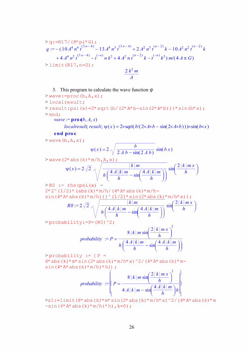
> q:=R17/(8*pi*G);

> limit(R17,n=0);

3. This program to calculate the wave function 𝜓

> wave:=proc(b,A,x);

> localresult;

> result:psi(x)=2*sqrt(b/(2*A*b-sin(2*A*b)))*sin(b*x);

> end;

> wave(b,A,x);

> wave(2*abs(k)*m/h,A,x);

> R0 := rhs(psi(x) = 2*2^(1/2)*(abs(k)*m/h/(4*A*abs(k)*m/h-

sin(4*A*abs(k)*m/h)))^(1/2)*sin(2*abs(k)*m/h*x));

> probability:=P=(R0)^2;

> probability := {P = 8*abs(k)*m*sin(2*abs(k)*m/h*x)^2/(4*A*abs(k)*m-

sin(4*A*abs(k)*m/h)*h)};

>s1:=limit(8*abs(k)*m*sin(2*abs(k)*m/h*x)^2/(4*A*abs(k)*m

-sin(4*A*abs(k)*m/h)*h),k=0);

q 10 A4 n4 t( )3 n 4

13 A4 n3 t( )3 n 4

2 A2 n3 t( )n 2

k 10 A2 n2 t( )n 2

k ( :=

4 A4 n2 t( )3 n 4

t( )n

n k2 4 A2 n t( )n 2

k t( )n

k2 ) m 4 A G/( )

2 k2 m

A

wave , ,b A xpro c( ) :=

; ;localresult result ( ) x 2 ( )sqrt /( )b 2 A b ( )sin 2 A b ( )sin b x

end pro c

( ) x 2b

2 A b ( )sin 2 A b( )sin b x

( ) x 2 2k m

h

4 A k m

h

sin

4 A k m

h

sin

2 k m x

h

:= R0 2 2k m

h

4 A k m

h

sin

4 A k m

h

sin

2 k m x

h

:= probability P

8 k m

sin

2 k m x

h

2

h

4 A k m

h

sin

4 A k m

h

:= probability

P

8 k m

sin

2 k m x

h

2

4 A k m

sin

4 A k m

hh

27

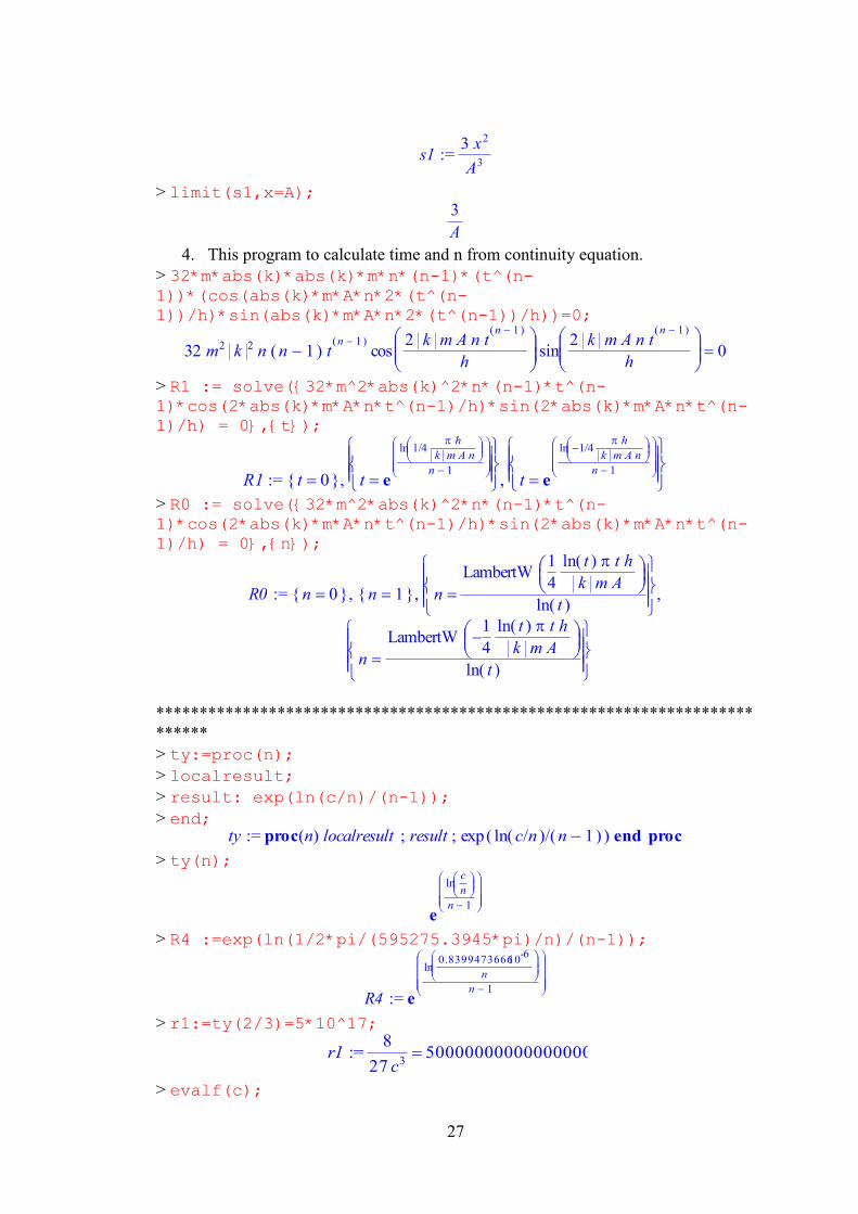
> limit(s1,x=A);

4. This program to calculate time and n from continuity equation.

> 32*m*abs(k)*abs(k)*m*n*(n-1)*(t^(n-

1))*(cos(abs(k)*m*A*n*2*(t^(n-

1))/h)*sin(abs(k)*m*A*n*2*(t^(n-1))/h))=0;

> R1 := solve({32*m^2*abs(k)^2*n*(n-1)*t^(n-1)*cos(2*abs(k)*m*A*n*t^(n-1)/h)*sin(2*abs(k)*m*A*n*t^(n-

1)/h) = 0},{t});

> R0 := solve({32*m^2*abs(k)^2*n*(n-1)*t^(n-1)*cos(2*abs(k)*m*A*n*t^(n-1)/h)*sin(2*abs(k)*m*A*n*t^(n-

1)/h) = 0},{n});

*********************************************************************

******

> ty:=proc(n);

> localresult;

> result: exp(ln(c/n)/(n-1));

> end;

> ty(n);

> R4 :=exp(ln(1/2*pi/(595275.3945*pi)/n)/(n-1));

> r1:=ty(2/3)=5*10^17;

> evalf(c);

:= s13 x2

A3

3

A

32 m2 k 2 n ( )n 1 t( )n 1

cos

2 k m A n t( )n 1

h

sin

2 k m A n t( )n 1

h0

:= R1 , ,{ }t 0

t e

ln /1 4

h

k m A n

n 1

t e

ln /1 4

h

k m A n

n 1

R0 { }n 0 { }n 1

n

LambertW

1

4

( )ln t t h

k m A

( )ln t, , , :=

n

LambertW

1

4

( )ln t t h

k m A

( )ln t

:= ty proc( ) end procn ; ;localresult result ( )exp /( )( )ln /c n n 1

e

ln

c

n

n 1

:= R4 e

ln

0.839947366610-6

n

n 1

:= r1 8

27 c3500000000000000000

28

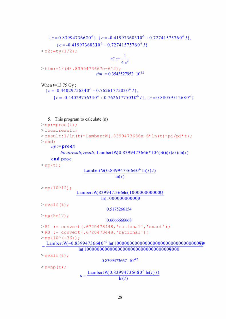
> r2:=ty(1/2);

> tim:=1/(4*.8399473667e-6^2);

When t=13.75 Gy ;

5. This program to calculate (n)

> np:=proc(t);

> localresult;

> result:1/ln(t)*LambertW(.8399473666e-6*ln(t)*pi/pi*t);

> end;

> np(t);

> np(10^12);

> evalf(%);

> np(5e17);

> R1 := convert(.6720473448,'rational','exact');

> R0 := convert(.6720473448,'rational');

> np(10^(-36));

> evalf(%);

> n=np(t);

{ }c 0.839947366710-6 { }c -0.419973683310-6 0.727415757610-6 I, ,

{ }c -0.419973683310-6 0.727415757610-6 I

:= r21

4 c2

:= tim 0.3543527952 1012

{ }c -0.440297563410-6 0.762617750310-6 I ,

{ }c -0.440297563410-6 0.762617750310-6 I { }c 0.880595126810-6,

np tpro c( ) :=

; ;localresult result /( )LambertW 0.8399473666*10^(-6) ( )ln t t ( )ln t

end pro c

( )LambertW 0.839947366610-6 ( )ln t t

( )ln t

( )LambertW 839947.3666 ( )ln 1000000000000

( )ln 1000000000000

0.5175266154

0.6666666668

( )LambertW 0.839947366610-42 ( )ln 1000000000000000000000000000000000000

( )ln 1000000000000000000000000000000000000

0.8399473667 10-42

n( )LambertW 0.839947366610-6 ( )ln t t

( )ln t

29

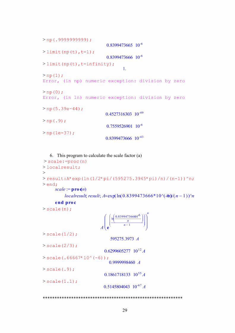
> np(.9999999999);

> limit(np(t),t=1);

> limit(np(t),t=infinity);

> np(1);

Error, (in np) numeric exception: division by zero

> np(0);

Error, (in ln) numeric exception: division by zero

> np(5.39e-44);

> np(.9);

> np(1e-37);

6. This program to calculate the scale factor (a)

> scale:=proc(n)

> localresult;

>

> result:A*exp(ln(1/2*pi/(595275.3945*pi)/n)/(n-1))^n;

> end;

> scale(n);

> scale(1/2);

> scale(2/3);

> scale(.66667*10^(-6));

> scale(.9);

> scale(1.1);

***********************************************************

0.8399473665 10-6

0.8399473666 10-6

1.

0.4527316303 10-49

0.7559526901 10-6

0.8399473666 10-43

scale npro c( ) :=

; ;localresult result A ^( )exp /( )( )ln /0.8399473666*10^(-6)n n 1 n

end pro c

A

e

ln

0.839947366610-6

n

n 1

n

595275.3973 A

0.6299605277 1012 A

0.9999998460 A

0.1861718133 1055 A

0.5145804043 10-67 A

30

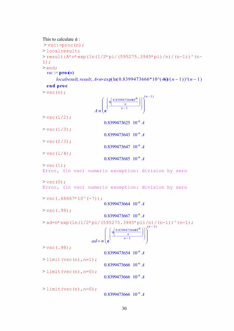
This to calculate 𝑎 : > vsc:=proc(n);

> localresult;

> result:A*n*exp(ln(1/2*pi/(595275.3945*pi)/n)/(n-1))^(n-1);

> end;

> vsc(n);

> vsc(1/2);

> vsc(1/3);

> vsc(2/3);

> vsc(1/4);

> vsc(1); Error, (in vsc) numeric exception: division by zero

> vsc(0); Error, (in vsc) numeric exception: division by zero

> vsc(.66667*10^(-7));

> vsc(.99);

> ad=n*exp(ln(1/2*pi/(595275.3945*pi)/n)/(n-1))^(n-1);

> vsc(.98);

> limit(vsc(n),n=1);

> limit(vsc(n),n=0);

> limit(vsc(n),n=0);

vsc npro c( ) :=

; ;localresult result A n ^( )exp /( )( )ln /0.8399473666*10^(-6)n n 1 ( )n 1

end pro c

A n

e

ln

0.839947366610-6

n

n 1

( )n 1

0.8399473625 10-6 A

0.8399473643 10-6 A

0.8399473647 10-6 A

0.8399473685 10-6 A

0.8399473664 10-6 A

0.8399473667 10-6 A

ad n

e

ln

0.839947366610-6

n

n 1

( )n 1

0.8399473654 10-6 A

0.8399473666 10-6 A

0.8399473666 10-6 A

0.8399473666 10-6 A

31

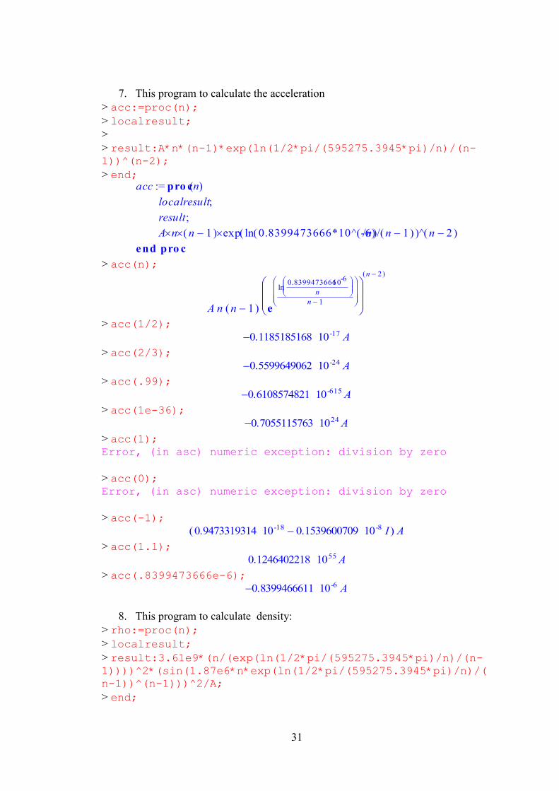
7. This program to calculate the acceleration

> acc:=proc(n);

> localresult;

>

> result:A*n*(n-1)*exp(ln(1/2*pi/(595275.3945*pi)/n)/(n-1))^(n-2);

> end;

> acc(n);

> acc(1/2);

> acc(2/3);

> acc(.99);

> acc(1e-36);

> acc(1); Error, (in asc) numeric exception: division by zero

> acc(0); Error, (in asc) numeric exception: division by zero

> acc(-1);

> acc(1.1);

> acc(.8399473666e-6);

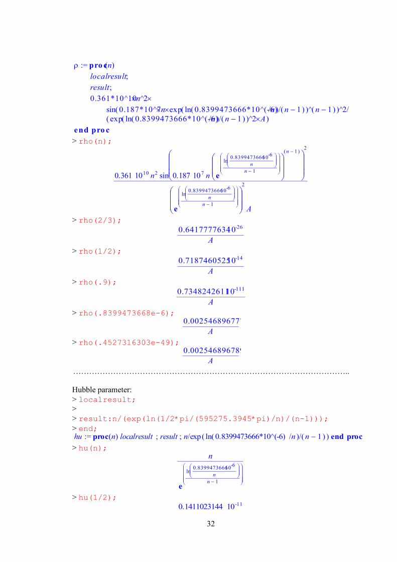
8. This program to calculate density:

> rho:=proc(n);

> localresult;

> result:3.61e9*(n/(exp(ln(1/2*pi/(595275.3945*pi)/n)/(n-

1))))^2*(sin(1.87e6*n*exp(ln(1/2*pi/(595275.3945*pi)/n)/(

n-1))^(n-1)))^2/A;

> end;

acc npro c( ) :=

localresult;

result;

A n ( )n 1 ^( )exp /( )( )ln /0.8399473666*10^(-6)n n 1 ( )n 2

end pro c

A n ( )n 1

e

ln

0.839947366610-6

n

n 1

( )n 2

0.1185185168 10-17 A

0.5599649062 10-24 A

0.6108574821 10-615 A

0.7055115763 1024 A

( )0.9473319314 10-18 0.1539600709 10-8 I A

0.1246402218 1055 A

0.8399466611 10-6 A

32

> rho(n);

> rho(2/3);

> rho(1/2);

> rho(.9);

> rho(.8399473668e-6);

> rho(.4527316303e-49);

…………………………………………………………………………………………..

Hubble parameter:

> localresult;

>

> result:n/(exp(ln(1/2*pi/(595275.3945*pi)/n)/(n-1)));

> end;

> hu(n);

> hu(1/2);

npro c( ) :=

localresult;

result;

0.361*10^10 ^n 2

^( )sin 0.187*10^7n ^( )exp /( )( )ln /0.8399473666*10^(-6)n n 1 ( )n 1 2/

^( )exp /( )( )ln /0.8399473666*10^(-6)n n 1 2 A( )

end pro c

0.361 1010 n2

sin 0.187 107 n

e

ln

0.839947366610-6

n

n 1

( )n 12

e

ln

0.839947366610-6

n

n 1

2

A

0.641777763410-26

A

0.718746052510-14

A

0.734824261110-111

A

0.002546896777

A

0.002546896789

A

:= hu proc( ) end procn ; ;localresult result /n ( )exp /( )( )ln /0.8399473666*10^(-6) n n 1

n

e

ln

0.839947366610-6

n

n 1

0.1411023144 10-11

33

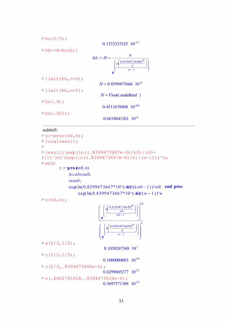
> hu(2/3);

> hh:=H=hu(n);

> limit(hh,n=0);

> limit(hh,n=1);

> hu(.9);

> hu(.001);

………………………………………………………………………………………

redshift:

> z:=proc(n0,n);

> localresult;

>

> result:(exp(ln((.8399473667e-6)/n0)/(n0-1)))^n0/(exp(ln((.8399473667e-6)/n)/(n-1)))^n;

> end;

> z(n0,n);

> z(2/3,1/2);

> z(2/3,1/3);

> z(2/3,.8399473666e-6);

> z(.6962745918,.8399473666e-6);

0.1333333325 10-17

:= hh Hn

e

ln

0.839947366610-6

n

n 1

H 0.8399473666 10-6

H ( )Float undefined

0.4511678498 10-60

0.6618041261 10-6

z ,n0 npro c( ) :=

localresult;

result;

^( )exp /( )( )ln /0.8399473667*10^(-6)n0 n0 1 n0/

^( )exp /( )( )ln /0.8399473667*10^(-6)n n 1 n

end proc

e

ln

0.839947366710-6

n0

n0 1

n0

e

ln

0.839947366710-6

n

n 1

n

0.1058267368 107

0.1000000003 1010

0.6299605277 1012

0.3697571388 1014

34

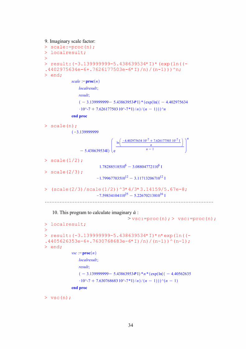
9. Imaginary scale factor: > scale:=proc(n); > localresult;

> > result:(-3.139999999-5.438639534*I)*(exp(ln((-

.4402975634e-6+.7626177503e-6*I)/n)/(n-1)))^n; > end;

> scale(n);

> scale(1/2);

> scale(2/3);

> (scale(2/3)/scale(1/2))^3*4/3*3.14159/5.67e-8;

…………………………………………………………………………………………

10. This program to calculate imaginary 𝑎 : > vsc:=proc(n); > vsc:=proc(n);

> localresult; >

> result:(-3.139999999-5.438639534*I)*n*exp(ln((-

.4405626353e-6+.7630768683e-6*I)/n)/(n-1))^(n-1); > end;

> vsc(n);

35

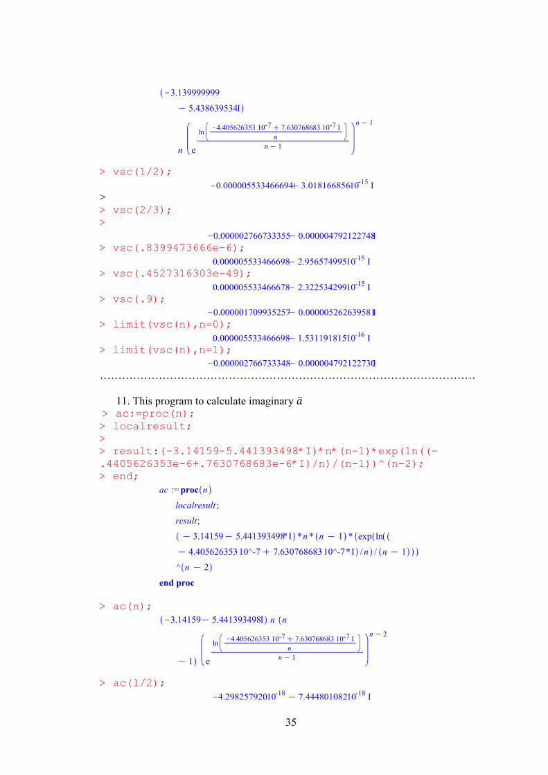
> vsc(1/2);

> > vsc(2/3); >

> vsc(.8399473666e-6);

> vsc(.4527316303e-49);

> vsc(.9);

> limit(vsc(n),n=0);

> limit(vsc(n),n=1);

…………………………………………………………………………………………

11. This program to calculate imaginary 𝑎 > ac:=proc(n);

> localresult; > > result:(-3.14159-5.441393498*I)*n*(n-1)*exp(ln((-

.4405626353e-6+.7630768683e-6*I)/n)/(n-1))^(n-2); > end;

> ac(n);

> ac(1/2);

36

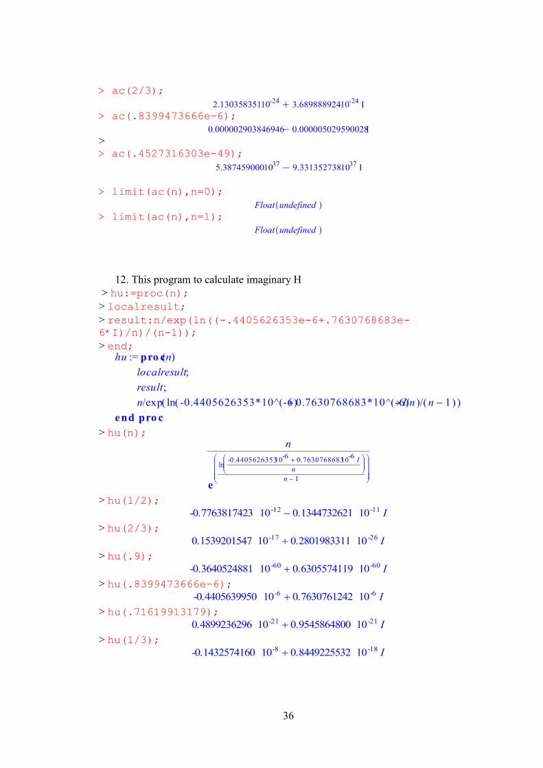
> ac(2/3);

> ac(.8399473666e-6);

> > ac(.4527316303e-49);

> limit(ac(n),n=0);

> limit(ac(n),n=1);

12. This program to calculate imaginary H

> hu:=proc(n);

> localresult;

> result:n/exp(ln((-.4405626353e-6+.7630768683e-6*I)/n)/(n-1));

> end;

> hu(n);

> hu(1/2);

> hu(2/3);

> hu(.9);

> hu(.8399473666e-6);

> hu(.71619913179);

> hu(1/3);

hu npro c( ) :=

localresult;

result;

/n ( )exp /( )( )ln /-0.4405626353*10^(-6) 0.7630768683*10^(-6)I n n 1

end pro c

n

e

ln

-0.440562635310-6

0.763076868310-6

I

n

n 1

-0.7763817423 10-12 0.1344732621 10-11 I

0.1539201547 10-17 0.2801983311 10-26 I

-0.3640524881 10-60 0.6305574119 10-60 I

-0.4405639950 10-6 0.7630761242 10-6 I

0.4899236296 10-21 0.9545864800 10-21 I

-0.1432574160 10-8 0.8449225532 10-18 I

37

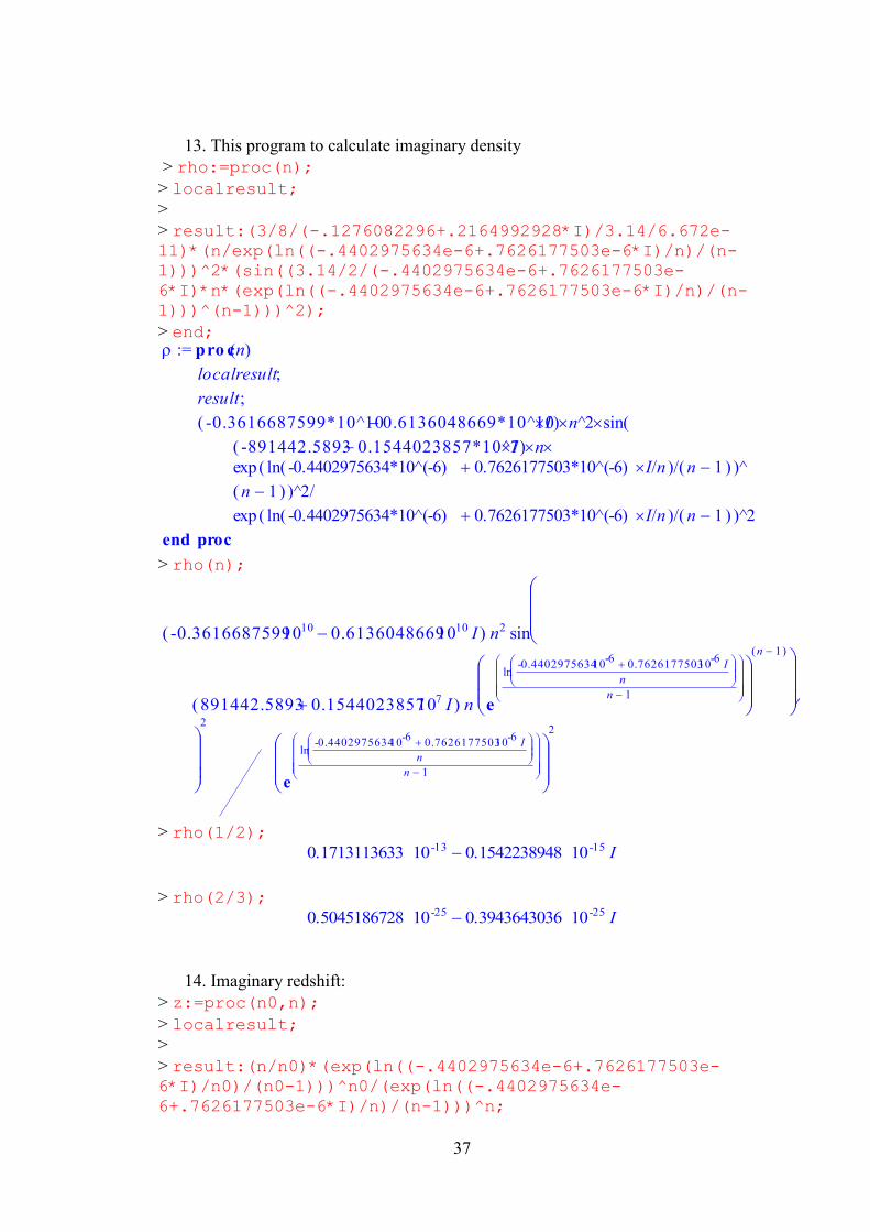
13. This program to calculate imaginary density

> rho:=proc(n);

> localresult;

>

> result:(3/8/(-.1276082296+.2164992928*I)/3.14/6.672e-11)*(n/exp(ln((-.4402975634e-6+.7626177503e-6*I)/n)/(n-

1)))^2*(sin((3.14/2/(-.4402975634e-6+.7626177503e-

6*I)*n*(exp(ln((-.4402975634e-6+.7626177503e-6*I)/n)/(n-

1)))^(n-1)))^2);

> end;

> rho(n);

> rho(1/2);

> rho(2/3);

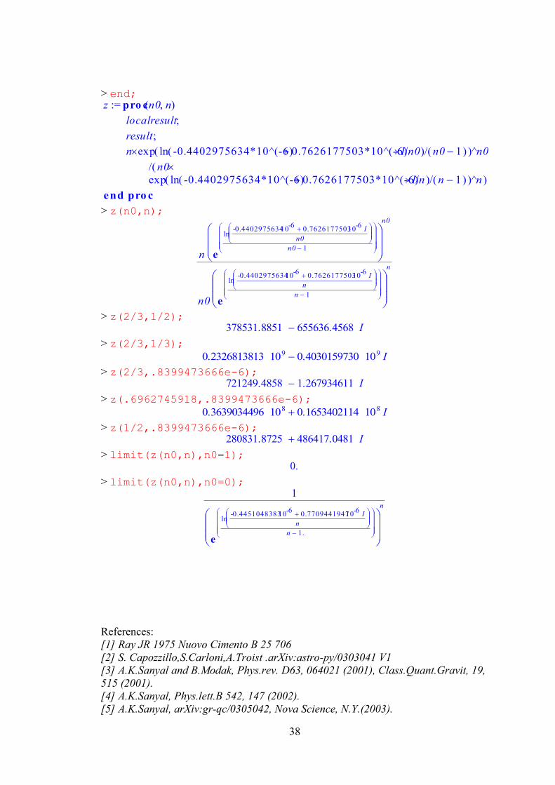
14. Imaginary redshift:

> z:=proc(n0,n);

> localresult;

>

> result:(n/n0)*(exp(ln((-.4402975634e-6+.7626177503e-6*I)/n0)/(n0-1)))^n0/(exp(ln((-.4402975634e-

6+.7626177503e-6*I)/n)/(n-1)))^n;

npro c( ) :=

localresult;

result;

( )-0.3616687599*10^10 0.6136048669*10^10I ^n 2 sin(

( )-891442.5893 0.1544023857*10^7I n

( )exp /( )( )ln /-0.4402975634*10^(-6) 0.7626177503*10^(-6) I n n 1 ^

( )n 1 ) 2^ /

^( )exp /( )( )ln /-0.4402975634*10^(-6) 0.7626177503*10^(-6) I n n 1 2

end proc

( )-0.36166875991010 0.61360486691010 I n2 sin

( )891442.5893 0.1544023857107 I n

e

ln

-0.440297563410-6

0.762617750310-6

I

n

n 1

( )n 1

^

2

e

ln

-0.440297563410-6

0.762617750310-6

I

n

n 1

2

0.1713113633 10-13 0.1542238948 10-15 I

0.5045186728 10-25 0.3943643036 10-25 I

38

> end;

> z(n0,n);

> z(2/3,1/2);

> z(2/3,1/3);

> z(2/3,.8399473666e-6);

> z(.6962745918,.8399473666e-6);

> z(1/2,.8399473666e-6);

> limit(z(n0,n),n0=1);

> limit(z(n0,n),n0=0);

References:

[1] Ray JR 1975 Nuovo Cimento B 25 706 [2] S. Capozzillo,S.Carloni,A.Troist .arXiv:astro-py/0303041 V1 [3] A.K.Sanyal and B.Modak, Phys.rev. D63, 064021 (2001), Class.Quant.Gravit, 19,

515 (2001). [4] A.K.Sanyal, Phys.lett.B 542, 147 (2002).

[5] A.K.Sanyal, arXiv:gr-qc/0305042, Nova Science, N.Y.(2003).

z ,n0 npro c( ) :=

localresult;

result;

n ^( )exp /( )( )ln /-0.4402975634*10^(-6) 0.7626177503*10^(-6)I n0 n0 1 n0

n0/(

^( )exp /( )( )ln /-0.4402975634*10^(-6) 0.7626177503*10^(-6)I n n 1 n )

end pro c

n

e

ln

-0.440297563410-6

0.762617750310-6

I

n0

n0 1

n0

n0

e

ln

-0.440297563410-6

0.762617750310-6

I

n

n 1

n

378531.8851 655636.4568 I

0.2326813813 109 0.4030159730 109 I

721249.4858 1.267934611 I

0.3639034496 108 0.1653402114 108 I

280831.8725 486417.0481 I

0.

1

e

ln

-0.445104838310-6

0.770944194710-6

I

n

n 1.

n

39

[6] D.Boulware, A.Strominger, E.T.Tomboulis, Quantum theory of gravity, Ed. S.

Christensen Adam Hilger, Bristol (1994). [7] M.Ostrogradski, Mem.Acad.St.Petersbourg Series 6, 385 (1950).

[8] A.K.Sanyal arXiv:hep-th/0407141 v1 16 Jul 2004

[9] G.T.Horowitz, Phys.Rev.D31,1169 (1985).

[10] A.A.Starobinsky, Phys.Lett.91B 99 (1980).

[11] A.A.Starobinsky and H.-J.Schmidt, Class.Q.Gravit.4 695 (1987) [12] K.Kucher, Quantum Gravity 2, ed. C.J.Isham, R.Penrose and D.W.Sciama,

Clarendon press. Oxford (1981) [13] L.O.Pimentel and O.Obregon, Class.Q.Gravit.11 2219(1994), L.O.Pimentel,

O.Obregon and J.J.Rosales, Class.Q.Gravit14379 (1997) [14] J.E.Lidsey, Class.Q.Gravit.11 2483 (1994)

[15] J.B.Hartle and S.Hawking, Phys.Rev.D288 2960 (1993)

[16] J.J.Halliwell and J.Louko Phys.Rev.D39 2206 (1989),

[17] H.-J.Schmidt, Phys.Rev.D49 6354 (1994)

[18] S.Hawking and J.C.Luttrell, Nucl.Phys.B247 250(1984)

[19] M.D.Pollock, Nucl.Phys.B306 931(1988)

[20] Carnegie Observatories Astrophysics Series, Vol. 2: Measuring and Modeling the Universe, 2004ed. W. L. Freedman (Cambridge:

Cambridge Univ. Press) [21] Capozziello S.,de Ritis R., Rubano C., and Scudellaro P., Int. journ. Mod. Phys.

D 4, 767(1995).