A Canonical Analysis of the Einstein-Hilbert Action in First Order Form

arX

iv:h

ep-t

h/06

0921

9v1

29

Sep

2006

A Canonical Analysis of the Einstein-Hilbert Action in First

Order Form

N. Kiriushcheva,1, ∗ S. V. Kuzmin,2, † and D. G. C. McKeon2, ‡

1Department of Mathematics, University of Western Ontario, London, N6A 5B7 Canada

2Department of Applied Mathematics,

University of Western Ontario, London, N6A 5B7 Canada

(Dated: February 2, 2008)

Abstract

Using the Dirac constraint formalism, we examine the canonical structure of the Einstein-Hilbert

action Sd = 116πG

∫

ddx√−gR, treating the metric gαβ and the symmetric affine connection Γλ

µν as

independent variables. For d > 2 tertiary constraints naturally arise; if these are all first class, there

are d(d−3) independent variables in phase space, the same number that a symmetric tensor gauge

field φµν possesses. If d = 2, the Hamiltonian becomes a linear combination of first class constraints

obeying an SO(2, 1) algebra. These constraints ensure that there are no independent degrees of

freedom. The transformation associated with the first class constraints is not a diffeomorphism

when d = 2; it is characterized by a symmetric matrix ξµν . We also show that the canonical

analysis is different if hαβ =√−g gαβ is used in place of gαβ as a dynamical variable when d = 2,

as in d dimensions, det hαβ = −(√−g)d−2. A comparison with the formalism used in the ADM

analysis of the Einstein-Hilbert action in first order form is made by applying this approach in the

two dimensional case with hαβ and Γλµν taken to be independent variables.

PACS numbers: 11.10.Ef; 04.06.Ds

∗Electronic address: [email protected]†Electronic address: [email protected]‡Electronic address: [email protected]

1

I. INTRODUCTION

The Einstein-Hilbert action

Sd =1

16πG

∫

ddx√−gR (1)

in d dimensions is known to have an exceptionally rich and complex structure. The invariance

of Sd under the diffeomorphism

x′λ = x′λ(xσ) (2)

implies that many of the apparent degrees of freedom present in Sd are in fact gauge artifacts.

A Cauchy analysis of the equations of motion that follow from (1) bears this out [1]. If one

were to make a weak field expansion

gµν(x) = ηµν +Gφµν(x) (3)

of the metric about the Minkowski metric ηµν , then Sd takes the form of a self interacting

spin two gauge theory. The diffeomorphism invariance of eq. (2) becomes in the weak field

limit

φµν(x) → φµν(x) + ∂µθν(x) + ∂νθµ(x). (4)

It can be shown that of the 12d(d+1) components of φµν , there are only 1

2d(d−3) degrees of

freedom that are physical, provided d ≥ 3 [2]. These may be identified with the transverse

and traceless part of φij. (Latin indices are spatial.) If d = 2, there are no degrees of freedom

associated with a spin two gauge field [3]. (This does not imply that the action is purely a

surface term; if g01 6= 0 in two dimensions√−gR is no longer a total derivative [32].)

Rather than analyzing Sd by use of the weak field expansion of eq. (3), it is possible to

employ the Dirac constraint analysis [4-6] to disentangle the canonical structure of Sd. This

has been done in a variety of ways. Two well known papers that deal with the canonical

structure of S4 are [7,8]. The canonical position variables in these papers are taken to be

gij, the metric on a spatial hypersurface. The components g0µ of the metric effectively

become Lagrange multiplier fields; the Hamiltonian is then a linear combination of first

class constraints. The Poisson brackets of these constraints are non local and have field

dependent structure constants, and hence do not form a Lie algebra [9]. The first class

constraints can be used to construct the generator of a gauge transformation [10]. This

generator is associated with a diffeomorphism transformation of g0µ [10]; the invariance

2

of gij under a diffeomorphism transformation on a space like surface is not broken in the

analysis of [7,8]. When a similar analysis is applied to S2, then the algebra of the Poisson

brackets associated with the first class constraints no longer has field dependent structure

constants, but still is non local and may acquire a central charge [11]. There are other

approaches to the canonical structure of Sd [12-14]; these generally entail using alternate

geometrical quantities as dynamical variables. We note that in these analyses, a condition

has been imposed on the metric which may serve to eliminate a gauge invariance that would

become apparent only if the canonical formalism is applied to the unrestricted action.

It was noticed by Einstein [15] that derivations of the equations of motion in Sd is sim-

plified if gµν and Γλµν are treated as being independent variables. If d 6= 2, the equation of

motion for Γλµν unambiguously gives

Γλµν =

1

2gλρ (gρµ,ν + gρν,µ − gµν,ρ) ≡

λ

µν

. (5)

(Often this approach is attributed to Palatini [16].) If d = 2 then we can only say that the

equation of motion for Γλµν implies that

Γλµν =

λ

µν

+ δλµξν + δλ

ν ξµ − gµνξλ (6)

where ξλ is an undetermined vector [17,18].

Treating gαβ and Γλµν as being independent can also simplify the canonical analysis of Sd

as then√−gR = hµν

(

Γλµν,λ − Γλ

λµ,ν + ΓλµνΓ

σσλ − Γλ

σµΓσλν

)

(7)

where

hµν =√−g gµν (8)

is the metric tensor density. (Eq. (7) can also be written in an alternate and possibly more

useful form√−gR = hµν

(

Gλµν,λ +

1

d− 1Gλ

λµGσσν −Gλ

σµGσλν

)

(9)

where Gλµν = Γλ

µν − 12

(

δλµΓσ

σν + δλν Γσ

σµ

)

.) It is apparent from eq. (7) that the Einstein-Hilbert

Lagrangian is at most linear in all derivatives with this choice of independent variables.

In the next section we examine the canonical structure of eq. (7) using the Dirac con-

straint formalism [4-6]. For d ≥ 3, some of the components of Γλµν which are independent

3

of time derivatives enter L nonlinearly so it is hard to completely disentangle the constraint

structure.

However, if d = 2 the Hamiltonian associated with L in (7) reduces to a linear combination

of constraints. The actual constraint structure when d = 2 is contingent upon whether gαβ

or hαβ is treated as independent, as by eq. (8)

det hαβ = −(√−g

)d−2. (10)

showing that when d = 2 it is not possible to express gαβ in terms of hαβ. In both cases

though the net number of degrees of freedom is zero. The quantization of this topological

action is treated in [19,20]. We discuss the canonical structure of S2 in first order form in

section three, showing how all degrees of freedom are constrained. (In [21,22], gravity in two

dimensions is treated as being over constrained.)

The canonical structure of the Einstein-Hilbert action described by [7,8] is derived from

the first order form of this action in d = 4 dimensions in [23,24]. In order to demonstrate

how this ADM analysis differs from what is being proposed here, we apply the ADM analysis

to S2 in section four, contrasting it to what is outlined in section three.

II. THE EINSTEIN-HILBERT LAGRANGIAN IN FIRST ORDER FORM

Though it is not necessary to do so, it is convenient to transfer derivatives occurring in√−gR as given in eq. (7) from the affine connections so that

Sd =∫

ddx[(

−Γ0ijh

ij)

+(

Γiji − Γ0

j0

)

hj + Γi0ih− Φ

(

hαβ ,Γλµν

)]

. (11)

(Latin indices are spatial, f denotes ∂tf and h = h00, hi = h0i.) Denoting momenta conjugate

to h by π and to Γ by Π, we have the primary constraints

Πµνλ = 0, πij = −Γ0

ij , πj = Γiji − Γ0

j0, π = Γi0i . (12 − 15)

If now

Λ = Γ000, Λk = Γk

00, Σi = Γjij . (16 − 18)

Σij = Γi

j0 −1

d− 1

(

Γkk0δ

ij

)

, Σijk = Γi

jk −1

d

(

δijΓ

ℓkℓ + δi

kΓℓjℓ

)

, (19 − 20)

then the function Φ in eq. (11) becomes

Φ = Λk(

h,k − hπk − 2hiπik

)

+ Λ(

−hi,i − πh+ hijπij

)

+ h

(

ΣijΣ

ji +

1

d− 1π2)

4

+hi

(

−2Σki,k +

d− 3

d− 1π,i + 2ππi − 2πΣi + 2Σk

ℓ Σℓki − 2

(d− 1)

dΣkΣ

ki

)

+hij

(

−Σkij,k +

2(d− 1)

dΣi,j − πi,j + πiπj − 2Σk

i πkj + ΣkℓiΣ

ℓkj + πkΣ

kij

−2(d− 1)

dΣiπj +

(d− 1)(d− 2)

d2ΣiΣj +

(

d− 3

d− 1

)

ππij − 2(d− 1)

dΣkΣ

kij

)

. (21)

The fields Λ, Λk, Σi, Σij and Σi

jk all have vanishing conjugate momenta which constitute a

set of additional primary constraints. Associated with these primary constraints are a set of

secondary constraints. The secondary constraints associated with the momenta conjugate

to the fields Λk and Λ are

χ = hi,i + hπ − hijπij , (22)

χk = h,k − hπk − 2hiπik. (23)

The usual Poisson brackets (PB) imply that these satisfy the closed algebra

{χi, χ} = χi {χi, χj} = 0. (24, 25)

The fields Σi, Σij and Σi

jk (collectively denoted by ~Σ) have equations of motion that lead

to additional constraints when d > 2. These fields enter into Φ in such a way that Φ can be

schematically written as

Φ = ~Λ · ~χ+1

2~ΣT M~Σ + ~Σ · ~v + Z. (26)

The momenta conjugate to the fields which contribute to ~Σ vanish; these primary constraints

lead to secondary constraints of the form

M~Σ + ~v = 0. (27)

From eq. (27), it is evident that if ~Σ has s components and if the rank of the matrix M is r,

then eq. (27) constitutes a set of r second class constraints and s− r first class constraints.

To determine the rank of M , we consider that portion of Φ given in eq. (21) that is bilinear

in ~Σ1:

Φ2 = hΣijΣ

ji + 2hi

(

Σkℓ Σ

ℓki −

(d− 1)

dΣkΣ

ki

)

+hij

(

ΣkℓiΣ

ℓkj +

(d− 1)(d− 2)

d2ΣiΣj −

2(d− 1)

dΣkΣ

kij

)

. (28)

In order to diagonalize Φ2 in the fields Σi, Σij and Σi

jk, we make the transformations

Σi → AhΣi (29)

5

Σij → BhΣi

j + C

(

hiΣj −1

d− 1δijh

kΣk

)

+DhkΣijk (30)

Σijk → EhΣi

jk. (31)

These transformations are consistent with Σij and Σi

jk being traceless. With the choice

D = −E, C = d−1dA and setting qij = h2hij − hhihj , we find that eq. (28) reduces to

Φ2 = B2h3ΣijΣ

ji + qij

[

d− 2

d− 1C2ΣiΣj +D2Σk

ℓiΣℓkj + 2CDΣkΣ

kij

]

, (32)

which, with Σijk = DΣi

jk + C(

δijΣk + δi

kΣj

)

, becomes

= B2h3ΣijΣ

ji + qij

(

ΣkℓiΣ

ℓkj −

d2

d− 1C2ΣiΣj

)

. (33)

It is evident once Φ2 is written in terms of these variables that the matrix M of eq. (26)

is invertible (i.e., the rank of this matrix equals its dimension). Consequently, all of the

equations of motion associated with the variables Σi, Σij and Σi

jk are second class constraints.

We now consider the number of variables and number of constraints we have encountered.

There are d(d+1)2

components of hµν and d2(d+1)2

components of Γλµν ; in total then there are

d(d+1)2

2independent fields. By eqs. (13-15), the momenta π, πi and πij and the momenta

Πij0 ,(

Πjii − Πj0

0

)

, Πi0i together generate d(d+1) second class constraints, while the vanishing

of momenta Π000 , Π00

k are by eqs. (16,17) a set of d first class constraints. In total, there

are [d − 1] + [d(d − 2)] + [12(d − 2)(d2 − 1)] = 1

2d(d2 − 3) variables Σi, Σi

j , Σijk; together

the equations of motion of the variables ~Σ and momenta associated with these ~Σ make up

d(d2 − 3) second class constraints.

We now assume that the d constraints χ, χk of eqs. (22,23) are all first class and that these

secondary constraints are responsible for a further set of d tertiary constraints which are

themselves first class, and which do not in turn generate further constraints. (Having χ, χk

being first class is consistent with eqs. (24,25) but it is necessary to see if they have vanishing

PB with the remaining secondary constraints.) In total then there are d + d + d = 3d first

class constraints and d(d+ 1) + d(d2 − 3) = d3 + d2 − 2d second class constraints. As these

3d first class constraints require the introduction of 3d additional constraints (the “gauge

conditions”), there would now be in total 3d+3d+(d3 +d2−2d) = d(d2 +d+4) restrictions

on the d(d+ 1)2 variables in phase space (the h’s, Γ’s and their associated momenta). This

would mean that there are d(d + 1)2 − d(d2 + d + 4) = d(d − 3) independent variables in

6

phase space. As has been noted in the introduction, this is the number of degrees of freedom

associated with a spin two gauge field in d dimensions. Consequently, although we have not

explicitly proven our assumptions about the secondary and tertiary constraints, we have

demonstrated that our assumptions are consistent in that the number of physical degrees of

freedom in d dimensions is the same as are present in a d dimensional spin two gauge theory.

It is possible that the sequence of 3d first class constraints (d primary, d secondary and

d tertiary) is associated with the d parameters that characterize the full four dimensional

diffeomorphism invariance of (1); the generator of this transformation can be found using

the formalism of [10]. The generator would involve d parameters on account of there being

d primary first class constraints, as well as the first and second time derivatives as there are

d secondary and d tertiary first class constraints following from these primary constraints.

The diffeomorphism transformation of eq. (2) gives rise to second derivatives of the gauge

parameters when the transformations of gαβ and Γλµν are considered. However, we are open

to the possibility that this procedure in fact leads to an invariance of the action of eq. (1)

that does not correspond to a diffeomorphism, as this is in fact what happens in d = 2

dimensions, as will be demonstrated below. In Ref. 25 it was noted that the portion of Eq.

(7) that is bilinear in g and Γ possesses an unusual invariance.

We will now turn our attention to d = 2 dimensions where the constraint structure

inherent in the Einstein-Hilbert action is more easily disentangled as the Hamiltonian is

now a linear combination of first class constraints.

III. THE TWO DIMENSIONAL ACTION

As has been emphasised in a number of papers [17,18,25,26] the first order formalism

when applied to the two dimensional Einstein-Hilbert action has some peculiar features.

In dimensions higher than two, either the metric gαβ or the metric density hαβ can be

used as dynamical variables as eq. (8) allows to pass from one to the other. However, in

two dimensions, if hαβ is used as a dynamical variable, then by eq. (10) we must have

det hαβ = −1 in order for the theory to be a metric theory. This can be ensured by

supplementing the action of eq. (7) with a Lagrange multiplier term

λΞ ≡ −λ(det hαβ + ρ). (34)

7

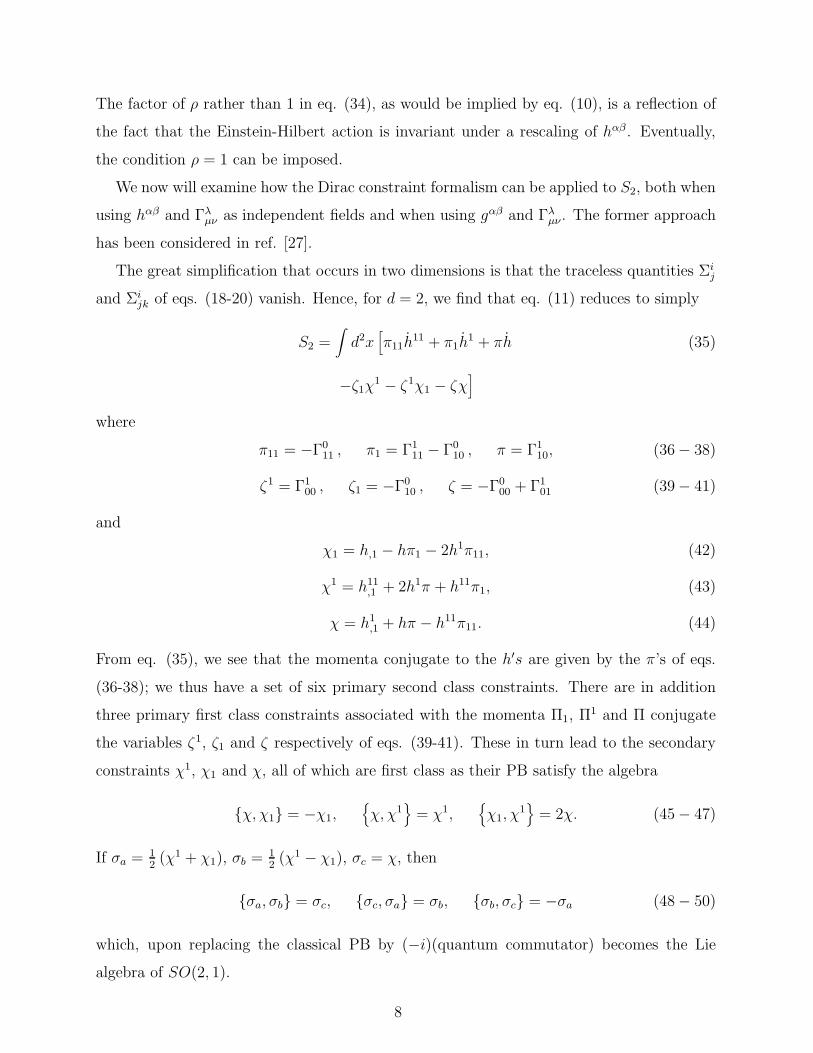
The factor of ρ rather than 1 in eq. (34), as would be implied by eq. (10), is a reflection of

the fact that the Einstein-Hilbert action is invariant under a rescaling of hαβ . Eventually,

the condition ρ = 1 can be imposed.

We now will examine how the Dirac constraint formalism can be applied to S2, both when

using hαβ and Γλµν as independent fields and when using gαβ and Γλ

µν . The former approach

has been considered in ref. [27].

The great simplification that occurs in two dimensions is that the traceless quantities Σij

and Σijk of eqs. (18-20) vanish. Hence, for d = 2, we find that eq. (11) reduces to simply

S2 =∫

d2x[

π11h11 + π1h

1 + πh (35)

−ζ1χ1 − ζ1χ1 − ζχ]

where

π11 = −Γ011 , π1 = Γ1

11 − Γ010 , π = Γ1

10, (36 − 38)

ζ1 = Γ100 , ζ1 = −Γ0

10 , ζ = −Γ000 + Γ1

01 (39 − 41)

and

χ1 = h,1 − hπ1 − 2h1π11, (42)

χ1 = h11,1 + 2h1π + h11π1, (43)

χ = h1,1 + hπ − h11π11. (44)

From eq. (35), we see that the momenta conjugate to the h′s are given by the π’s of eqs.

(36-38); we thus have a set of six primary second class constraints. There are in addition

three primary first class constraints associated with the momenta Π1, Π1 and Π conjugate

the variables ζ1, ζ1 and ζ respectively of eqs. (39-41). These in turn lead to the secondary

constraints χ1, χ1 and χ, all of which are first class as their PB satisfy the algebra

{χ, χ1} = −χ1,{

χ, χ1}

= χ1,{

χ1, χ1}

= 2χ. (45 − 47)

If σa = 12(χ1 + χ1), σb = 1

2(χ1 − χ1), σc = χ, then

{σa, σb} = σc, {σc, σa} = σb, {σb, σc} = −σa (48 − 50)

which, upon replacing the classical PB by (−i)(quantum commutator) becomes the Lie

algebra of SO(2, 1).

8

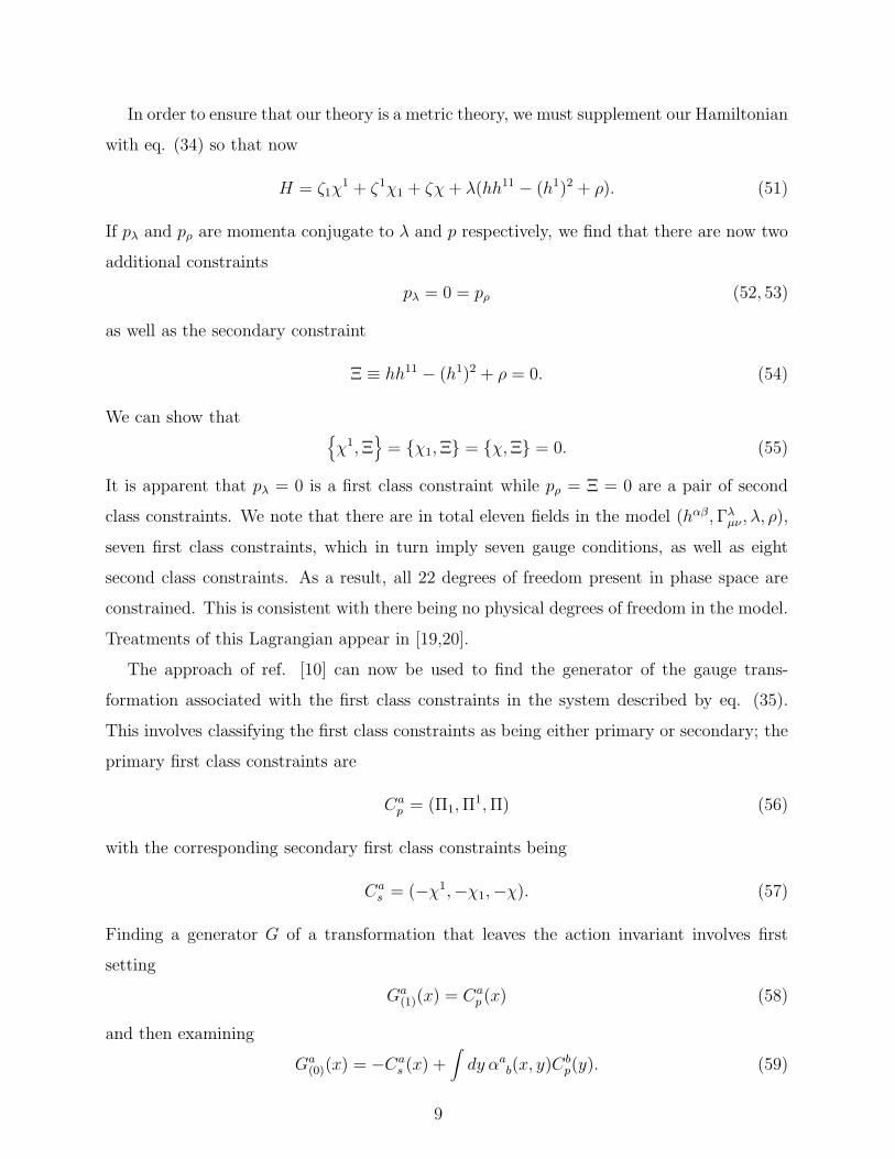
In order to ensure that our theory is a metric theory, we must supplement our Hamiltonian

with eq. (34) so that now

H = ζ1χ1 + ζ1χ1 + ζχ+ λ(hh11 − (h1)2 + ρ). (51)

If pλ and pρ are momenta conjugate to λ and p respectively, we find that there are now two

additional constraints

pλ = 0 = pρ (52, 53)

as well as the secondary constraint

Ξ ≡ hh11 − (h1)2 + ρ = 0. (54)

We can show that{

χ1,Ξ}

= {χ1,Ξ} = {χ,Ξ} = 0. (55)

It is apparent that pλ = 0 is a first class constraint while pρ = Ξ = 0 are a pair of second

class constraints. We note that there are in total eleven fields in the model (hαβ,Γλµν , λ, ρ),

seven first class constraints, which in turn imply seven gauge conditions, as well as eight

second class constraints. As a result, all 22 degrees of freedom present in phase space are

constrained. This is consistent with there being no physical degrees of freedom in the model.

Treatments of this Lagrangian appear in [19,20].

The approach of ref. [10] can now be used to find the generator of the gauge trans-

formation associated with the first class constraints in the system described by eq. (35).

This involves classifying the first class constraints as being either primary or secondary; the

primary first class constraints are

Cap = (Π1,Π

1,Π) (56)

with the corresponding secondary first class constraints being

Cas = (−χ1,−χ1,−χ). (57)

Finding a generator G of a transformation that leaves the action invariant involves first

setting

Ga(1)(x) = Ca

p (x) (58)

and then examining

Ga(0)(x) = −Ca

s (x) +∫

dy αab(x, y)C

bp(y). (59)

9

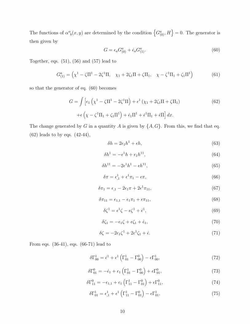
The functions of ααb(x, y) are determined by the condition

{

Ga(0), H

}

= 0. The generator is

then given by

G = ǫaGa(0) + ǫaG

a(1). (60)

Together, eqs. (51), (56) and (57) lead to

Ga(1) =

(

χ1 − ζΠ1 − 2ζ1Π, χ1 + 2ζ1Π + ζΠ1, χ− ζ1Π1 + ζ1Π1)

(61)

so that the generator of eq. (60) becomes

G =∫

[

ǫ1(

χ1 − ζΠ1 − 2ζ1Π)

+ ǫ1 (χ1 + 2ζ1Π + ζΠ1) (62)

+ǫ(

χ− ζ1Π1 + ζ1Π1)

+ ǫ1Π1 + ǫ1Π1 + ǫΠ

]

dx.

The change generated by G in a quantity A is given by {A,G}. From this, we find that eq.

(62) leads to by eqs. (42-44),

δh = 2ǫ1h1 + ǫh, (63)

δh1 = −ǫ1h+ ǫ1h11, (64)

δh11 = −2ǫ1h1 − ǫh11, (65)

δπ = ǫ1,1 + ǫ1π1 − ǫπ, (66)

δπ1 = ǫ,1 − 2ǫ1π + 2ǫ1π11, (67)

δπ11 = ǫ1,1 − ǫ1π1 + ǫπ11, (68)

δζ1 = ǫ1ζ − ǫζ1 + ǫ1, (69)

δζ1 = −ǫ1ζ + ǫζ1 + ǫ1, (70)

δζ = −2ǫ1ζ1 + 2ǫ1ζ1 + ǫ. (71)

From eqs. (36-41), eqs. (66-71) lead to

δΓ100 = ǫ1 + ǫ1

(

Γ101 − Γ0

00

)

− ǫΓ100, (72)

δΓ001 = −ǫ1 + ǫ1

(

Γ101 − Γ0

00

)

+ ǫΓ001, (73)

δΓ011 = −ǫ1,1 + ǫ1

(

Γ111 − Γ0

01

)

+ ǫΓ011, (74)

δΓ101 = ǫ1,1 + ǫ1

(

Γ111 − Γ0

01

)

− ǫΓ101, (75)

10

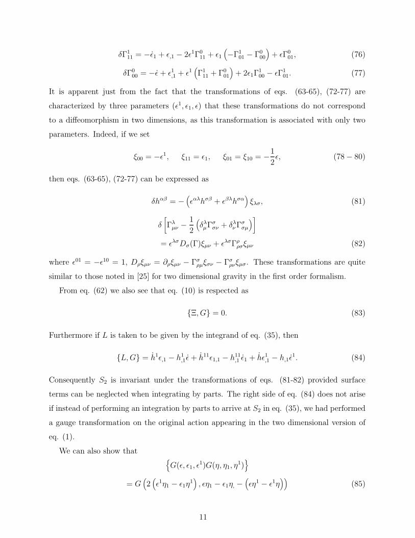
δΓ111 = −ǫ1 + ǫ,1 − 2ǫ1Γ0

11 + ǫ1(

−Γ101 − Γ0

00

)

+ ǫΓ001, (76)

δΓ000 = −ǫ+ ǫ1,1 + ǫ1

(

Γ111 + Γ0

01

)

+ 2ǫ1Γ100 − ǫΓ1

01. (77)

It is apparent just from the fact that the transformations of eqs. (63-65), (72-77) are

characterized by three parameters (ǫ1, ǫ1, ǫ) that these transformations do not correspond

to a diffeomorphism in two dimensions, as this transformation is associated with only two

parameters. Indeed, if we set

ξ00 = −ǫ1, ξ11 = ǫ1, ξ01 = ξ10 = −1

2ǫ, (78 − 80)

then eqs. (63-65), (72-77) can be expressed as

δhαβ = −(

ǫαλhσβ + ǫβλhσα)

ξλσ, (81)

δ

[

Γλµν −

1

2

(

δλµΓσ

σν + δλν Γσ

σµ

)

]

= ǫλσDσ(Γ)ξµν + ǫλσΓρρσξµν (82)

where ǫ01 = −ǫ10 = 1, Dρξµν = ∂ρξµν − Γσρµξσν − Γσ

ρνξµσ. These transformations are quite

similar to those noted in [25] for two dimensional gravity in the first order formalism.

From eq. (62) we also see that eq. (10) is respected as

{Ξ, G} = 0. (83)

Furthermore if L is taken to be given by the integrand of eq. (35), then

{L,G} = h1ǫ,1 − h1,1ǫ+ h11ǫ1,1 − h11

,1 ǫ1 + hǫ1,1 − h,1ǫ1. (84)

Consequently S2 is invariant under the transformations of eqs. (81-82) provided surface

terms can be neglected when integrating by parts. The right side of eq. (84) does not arise

if instead of performing an integration by parts to arrive at S2 in eq. (35), we had performed

a gauge transformation on the original action appearing in the two dimensional version of

eq. (1).

We can also show that{

G(ǫ, ǫ1, ǫ1)G(η, η1, η

1)}

= G(

2(

ǫ1η1 − ǫ1η1)

, ǫη1 − ǫ1η, −(

ǫη1 − ǫ1η))

(85)

11

so that the generator of the transformation of eqs. (81,82) satisfies a closed algebra. Its

structure is the same as that of eqs. (45-47). We thus see that the gauge generator satisfies

a local closed algebra with field independent structure constants. In this, the two dimen-

sional Einstein-Hilbert action more closely resembles non-Abelian gauge theory than the

four dimensional Einstein-Hilbert action when analyzed using the Dirac-ADM [7-9] analysis

of constraints.

We now consider how the two dimensional Einstein-Hilbert action can be treated if gαβ

and Γλµν are taken to be the canonical “position” variables in place of hαβ and Γλ

µν . This

eliminates the need to impose the condition of eq. (10) “by hand” in order for the theory to

be a metric theory. It also permits supplementing the action S2 with a cosmological term

Λ∫

d2x√−g. This term cannot be expressed in terms of hαβ in two dimensions.

We now find it convenient to write S2 in the form

S2 =∫

d2x[

h11ξ11 + h1ξ1 + hξ −[

ζ1(

h,1 + hξ1 + 2h1ξ11)

+ζ1(

h11,1 − 2h1ξ − h11ξ1

)

+ ζ(

h1,1 − hξ + h11ξ11

)]]

, (86)

where

ξ11 = Γ011, ξ1 = Γ0

01 − Γ111, ξ = −Γ1

01 (87 − 89)

and now h11, h1 and h are not independent variables but are defined by the equations

h11 =√−g g11, h1 =

√−g g01, h =

√−g g00. (90 − 92)

In this form, we have the canonical momenta

π11 =∂L

∂ξ11=

√−g g11, π1 =∂L

∂ξ1=

√−g g01, π =∂L

∂ξ=

√−g g00, (93 − 95)

p11 =∂L

∂g11= 0, p1 =

∂L

∂g01= 0, p =

∂L

∂g00= 0, (96 − 98)

Π1 =∂L

∂ζ1= 0, Π1 =

∂L

∂ζ1= 0, Π =

∂L

∂ζ. (99 − 101)

These are all primary constraints. The constraints of eq. (99-101) are all first class. Those

of eqs. (93-98) are not all second class, as is apparent from the fact that the matrix formed

by the PB of these constraints is of rank four, not six. This is on account of eq. (10) which

implies that if (93-95) are satisfied then

Ξ11π = ππ11 − (π1)2 + 1 = 0. (102)

12

There are in addition the secondary constraints

χ1 = π,1 + πξ1 + 2π1ξ11 = 0, (103)

χ1 = π11,1 − 2π1ξ − π11ξ1 = 0, (104)

χ = π1,1 − πξ + π11ξ11 = 0. (105)

When eq. (102) is satisfied, then the three constraints of eqs. (103-105) are no longer

independent as now

π11χ1 + πχ1 − 2π1χ = 0 . (106)

We could take four of the six constraints of eqs. (93-98) as being second class and the

remaining two to be first class; eqs. (99-101) would constitute an additional three first class

constraints. Finally, two of the three constraints of eqs. (103-105) would be first class. In

total then, there are four second class constraints and seven first class constraints. When

these are combined with seven gauge conditions, there are in total 4+7+7 = 18 restrictions

on the 18 variables gαβ, Γλµν and their conjugate momenta.

In place of taking two of the constraints of eq. (93-98) to be first class, we instead find it

convenient to take eq. (102) to be first class along with all of the constraints of eqs. (103-

105). There are still seven first class constraints and no degrees of freedom. The constraints

of eqs. (103-105) satisfy the algebra of eqs. (45-47) and have a vanishing PB with the

constraint Ξ11π of eq. (102).

The approach of Castellani [10] can again be used to find the generator of the gauge trans-

formation associated with first class constraints of eqs. (99-105). Following the approach

that led to G in eq. (62), we arrive at

G =∫

[

ǫ(

χ− ζ1Π1 + ζ1Π1)

+ ǫ1(

χ1 − 2ζ1Π − ζΠ1)

+ǫ1 (χ1 + 2ζ1Π + ζΠ1) + ǫΠ + ǫ1Π1 + ǫ1Π1 + ǫ11Ξ

11π

]

dx. (107)

From eq. (107), we recover the transformations of eqs. (63-65), (72-77) with the additional

transformations

δΓ011 = ǫ11π, (108)

δΓ101 = −ǫ11π11, (109)

δΓ111 = 2ǫ11π

1, (110)

13

δΓ000 = −ǫ11π11. (111)

With L now given by

L = π11ξ11 + π1ξ1 + πξ −(

ζ1χ1 + ζ1χ1 + ζχ

)

(112)

then it follows that

{L,G} = ǫ1,1π − ǫ1π,1 + ǫ1,1π − ǫ1π11,1 + ǫ,1π

1 − ǫπ1,1

− d

dt

[

ǫ1(

πξ1 + 2π1ξ11)

+ ǫ1(

−2π1ξ − π11ξ1)

+ ǫ(

−πξ + π11ξ11)]

− ǫ11d

dt(Ξ11

π ), (113)

so that provided surface terms can be neglected and eq. (102) is satisfied, the action S2 is

invariant.

A more direct approach is to select two of the six constraints following from eqs. (93-98)

to be first class and use the remaining four second class constraints to explicitly eliminate

four degrees of freedom. If we take eqs. (94,95, 97, 98) to be second class constraints, we

have the strong equations

p = 0 = p1, (114 − 115)

g00 = − π2

1 − (π1)2g11, g01 = − ππ1

1 − (π1)2g11 (116 − 117)

so that g00 and g01 are expressed in terms of π, π1 and g11.

The remaining five primary first class constraints present in eqs. (93-101) can now be

written using these strong equations as

Π1 = Π1 = Π = 0, p11 = 0, π11 =−1 + (π1)2

π. (118 − 122)

Furthermore, the action of eq. (86) now can be expressed as

S2 =∫

d2x

{(

−1 + (π1)2

π

)

ξ11 + π1ξ1 + πξ (123)

−[

ζ1(

π,1 + πξ1 + 2π1ξ11)

+ζ1

(

−1 + (π1)2

π

)

,1

− 2π1ξ −(

−1 + (π1)2

π

)

ξ1

+ζ

(

π1,1 − πξ + (

−1 + (π1)2

π

)

ξ11

)]}

.

14

The first three constraints of eqs. (118-122) are primary constraints that lead to the sec-

ondary first class constraints

χ1 = π,1 + πξ1 + 2π1ξ11, (124)

χ1 =

(

−1 + (π1)2

π

)

,1

− 2π1ξ −(

−1 + (π1)2

π

)

ξ1, (125)

χ = π1,1 − πξ +

(

−1 + (π1)2

π

)

ξ11. (126)

These constraints are not independent as they satisfy eq. (106) automatically. They also

obey the algebra of eqs. (45-47). If χ and χ1 are taken to be independent, we then have

χ1 =1

π

(

2π1χ− −1 + (π1)2

πχ1

)

(127)

as the dependent secondary constraint.

Together, the seven first class constraints (five primary given by eqs. (118-122) and two

secondary −χ and −χ1 result in a gauge generator

G =∫

dx

[

ǫ11p11 + ǫ11

(

π11 +−1 + (π1)2

π

)

+ ǫ1(

χ1 − ζΠ1 − 2ζ1Π)

+ǫ1 (χ1 + 2ζ1Π + ζΠ1) + ǫ(

χ− ζ1Π1 + ζ1Π1)

+ǫ1Π1 + ǫ1Π1 + ǫΠ

]

. (128)

In deriving eq. (128) using the approach of ref. [10], we have treated the secondary con-

straints of eqs. (124-126) as independent though they are related by eq. (127); strictly

speaking the approach of ref. [10] assumes that the secondary constraints are not depen-

dent. Despite this, G of eq. (128) is consistent with invariances of S2 in eq. (123).

Keeping in mind eqs. (124-126) we find that G satisfies the algebra of eq. (85). The

changes in the dynamical variables induced by G now take the form

δg11 = ǫ11 (129)

(This reflects the fact that S2 in eq. (123) is independent of g11.),

δg00 = ǫ11g00

g11+ 2ǫg00 + 2ǫ1

g00g01

g11− 2ǫ1g

01, (130)

δg01 = ǫ11g01

g11+ ǫg01 +

2ǫ1(g01)2

g11− ǫ1g

11 − ǫ1g00, (131)

15

δΓ100 = ǫ1 − ǫΓ1

00 + ǫ1(

Γ101 − Γ0

00

)

, (132)

δΓ001 = ǫ1 + ǫΓ0

01 − ǫ1(

Γ101 − Γ0

00

)

, (133)

δΓ101 = ǫ1,1 − ǫ1

(

Γ001 − Γ1

11

)

− ǫΓ101 −

g11

g00

(

ǫ11 − ǫΓ011 − ǫ1,1 − ǫ1

(

Γ001 − Γ1

11

))

, (134)

δΓ011 = ǫ11, (135)

δΓ000 = ǫ1,1 + ǫ1

(

Γ001 + Γ1

11

)

− ǫΓ101 −

g11

g00

(

ǫ11 − ǫΓ011 − ǫ1,1 − ǫ1

(

Γ001 − Γ1

11

))

−ǫ− 2ǫ1Γ100, (136)

δΓ111 = ǫ1 + ǫΓ0

01 + ǫ1(

Γ101 + Γ0

00

)

+ ǫ,1 − 2ǫ1Γ011 +

2g01

g00

(

ǫ11 − ǫΓ011

−ǫ1,1 − ǫ1(

Γ001 − Γ1

11

))

. (137)

It is not clear if there is a relationship between the transformations of eqs. (132-137) and

those of eqs. (72-77, 108-111), though eqs. (63-65) are consistent with eqs. (129-131).

We now turn to examining how the ADM approach to the canonical analysis of the

Einstein-Hilbert action expressed in first order form is related to what has been done above.

IV. THE ADM APPROACH

The canonical analysis of the four dimensional Einstein-Hilbert action in refs. [7,8] was

originally performed using gαβ as the only dynamical variable; Γλµν was given by the Christof-

fel symbol in this analysis. (For reviews of this approach, see for example [9,28,29].)

The ADM canonical Hamiltonian is also derived in the first order formalism with gαβ

and Γλµν being treated as independent variables in [23,24]. This analysis differs from what

appears in section 2 above by using the four secondary constraints of eqs. (22-23) as well

as the 26 constraints following from the equations of motion of the variables Σi, Σij and

Σijk to eliminate in total 30 of the 50 variables appearing in the original Lagrangian (10

components of gαβ and 40 components of Γλµν). However, when these equations are used,

the coefficients of the four variables Λ and Λk appearing in eq. (21) all vanish, and hence

the Lagrangian analyzed in the ADM approach only contains 50-30-4 = 16 variables; these

are gµν and Γ0ij. Four of the components of gµν appear as Lagrange multipliers in the

Hamiltonian; the six remaining components of gµν have canonical momenta composed of

the components of Γ0ij. There are thus 20 variables in all in phase space when the momenta

16

ΠA conjugate to the Lagrange multipliers A = (Λ,Λk) are considered in addition to the

16 variables appearing explicitly in the Lagrangian. There consequently are four primary

constraints (the momenta ΠA vanish) and four secondary constraints (the coefficients of the

Lagrange multipliers). These eight constraints are all first class; when combined with eight

gauge conditions there are 20-8-8=4 independent degrees of freedom in phase space. These

are the two propagating modes of the graviton plus their conjugate momenta. The four

primary and four secondary first class constraints can be used to form the generator of a

gauge transformation [10].

In sections two and three above we have not used equations of motion that are independent

of time derivatives to eliminate dynamical variables. Indeed, by using equations of motion

associated with first class constraints it is inevitable that some information about the gauge

invariance present in the initial Lagrangian would be lost. Furthermore, tertiary constraints

will not arise, and if these are first class, even more information is lost. Indeed, having

only 16 of the original 50 degrees of freedom left in the Lagrangian after using the time

independent equations of motion means that only by employing the equations of motion in

conjunction with the generator of the gauge transformation can the transformation of all 50

fields gαβ and Γλµν be found. (We note that in analyzing the canonical structure of the four

dimensional Einstein-Hilbert Lagrangian when expressed in terms of the vierbein and spin

connection, it is not necessary to employ equations of motion [12].)

Let us explicitly demonstrate what happens when the approach to the Einstein-Hilbert

Lagrangian in four dimensions used in [23,24] is applied to the action S2 in eq. (35). In this

case, the variables ζ1, ζ1 and ζ do not enter with time derivatives and hence their equations

of motion show that χ1, χ1 and χ vanish where these quantities are defined by eqs. (42-44).

They also satisfy the restriction that

h11χ1 + hχ1 − 2h1χ = (hh11 − (h1)2),1. (138)

On account of eq. (138), it is not possible to solve these equations of motion for all of π11,

π1 and π. However, if we use χ1 = χ1 = 0 we find that

π11 =1

2h1(h,1 − hπ1) , (139)

π =−1

2h1

(

h11,1 + h11π1

)

. (140)

17

Substitution of eqs. (139-140) into eq. (44) leads to

χ =1

2h1

(

(

h1)2 − hh11

)

,1(141)

and eq. (35) reduces to

S2 =∫

d2x

[

1

2h1

(

h,1h11 − h11

,1 h)

+π1

2h1

d

dt

(

(

h1)2 − hh11

)

− ζ

2h1

(

(

h1)2 − hh11 + k

)

,1

]

.

(142)

(We are free to add a constant k in eq. (142) as indicated.) The first term in eq. (142)

cancels against the second term upon integrating by parts. If now we set

H11 =π1

2h1H11 = −

(

ζ

2h1

)

,1

(143)

then eq. (142) reduces to

S2 =∫

d2x[

H11

(

2h1h1 − h11h− hh11)

(144)

−H11

(

(

h1)2 − hh11 + k

)]

.

We thus have the primary constraints

ψ1 ≡ π1 − 2h1H11 = 0 , ψ ≡ π + h11H11 , ψ11 ≡ π11 + hH11 , (145 − 147)

and

Π11 = 0 = Π11 (148 − 149)

for the momenta π1 . . .Π11 conjugate to h1 . . . H11 respectively. There is one secondary

constraint

Ξ11 = (h1)2 − hh11 + k. (150)

The equations

{

ψ1,Ξ11}

= −2h1,{

ψ1,Ξ11}

= h11,{

ψ11,Ξ11}

= h (151 − 153)

show that there are four first class constraints which we take to be

Π11 = Π11 = 0 (154 − 155)

hψ + h11ψ11 + h1ψ1 = hψ − h11ψ11 = 0 (156 − 157)

18

and two second class constraints, for which we choose

ψ1 = Ξ11 = 0. (158 − 159)

Once four gauge conditions are chosen, all ten degrees of freedom associated with h, h1, h11,

H11, H11 and their conjugate momenta are fixed.

The four first class constraints of eqs. (154-157) are all primary, so the gauge generator

is simply [10]

GI =∫

[

ǫ11Π11 + ǫ11Π

11 + ǫa(

hψ + h11ψ11 + h1ψ1

)

+ ǫb(

hψ − h11ψ11

)]

dx. (160)

It is also possible to consider the constraints Π11, ψ1, ψ and Ξ11 to be first class and Π11

and ψ11 to be second class. This entails using ψ11 = 0 to express

H11 = −−π11

h, (161)

so that we write now

ψ1 = π1 +2h1π11

h, (162)

ψ = π − h11

hπ11. (163)

Since Ξ11 is a secondary constraint associated with the primary constraint Π11, the gauge

generator now becomes

GII =∫

[

ǫ1ψ1 + ǫψ + ǫ11Ξ11 + ˙ǫ11Π

11]

dx. (164)

From eqs. (160) and (144), we see that

{GI , L} =

[

−ǫ11d

dt− ǫ11 + (2H11ǫa)

d

dt

]

Ξ11, (165)

so that on the constraint surface, L is gauge invariant under the transformation generated

by eq. (160). So also, the generator of eq. (164) leaves S2 of eq. (144) invariant on the

constraint surface.

V. DISCUSSION

In this paper, we have examined the canonical structure of the Einstein-Hilbert action

when written in first order form, using the metric and affine connection as independent

19

variables. The algebraic complexity that arises when applying the Dirac constraint formalism

in d > 2 dimensions prevents us from fully implementing this way of disentangling the

structure of these actions. However, when d = 2 it has proved possible to determine all

constraints, both using the metric density hαβ and the metric gαβ as dynamical variables.

In the former case, a new symmetry (given by eqs. (81,82)) is derived. Furthermore, in two

dimensions the algebra of constraints is local with field independent structure constants; it

is tempting to speculate that these features persist in higher dimensions. The structure of

eq. (9) suggests that this formalism may be simpler to implement when using Gλµν in place

of Γλµν . (The use of Gλ

µν will be outlined elsewhere.)

Completing the analysis of the Einstein-Hilbert action in d > 2 dimensions along the lines

proposed in section 3 is clearly a priority. Another problem that suggests itself is to fully

quantize the two dimensional Einstein-Hilbert action when using the first order formalism of

section 4 [33]. Despite the fact that the constraints serve to eliminate all canonical degrees

of freedom in this model, the structure of such theories can be of interest [19,20,30]. It would

also be worth considering what happens to the canonical structure of the two dimensional

Einstein-Hilbert actions if it were supplemented by a cosmological term or matter fields.

Its structures when written in terms of the zweibein and spin connection (as in [12]) also

merits attention. The use of these variables has been explored in [31]; it has been found that

tertiary constraints in fact arise in this approach, consistent with our own expectations.

VI. ACKNOWLEDGEMENTS

D.G.C.McKeon would like to thank NSERC for financial support and R. and D. MacKen-

zie for useful suggestions.

[1] A. Lichnerowicz, Theories relativistes de la gravitation et de l’ electromagnetisme (Masson,

Paris, 1955).

[2] M. Fierz and W. Pauli, Proc. Roy. Soc. London, Ser. A, 173, 211 (1939).

[3] D.G.C. McKeon and T.N. Sherry, Journal of Phys. A23, 4691 (1990).

[4] P.A.M. Dirac, Can. J. Math. 2, 129 (1950).

[5] P.A.M. Dirac, Proc. Roy. Soc. A 246, 326 (1958).

20

[6] P.A.M. Dirac, Lectures on Quantum Mechanics (Dover Mineola, 2001).

[7] P.A.M. Dirac, Proc. Roy. Soc. A 246, 333 (1958).

[8] R. Arnowitt, S. Deser and C.W. Misner, in Gravitation: An Introduction to Current Research

Edited by L. Witten, (Wiley, New York, 1962).

[9] C. Teitelboim, The Hamilton Structure of Space Time (Princeton notes, 1978, unpublished).

[10] L. Castellani, Ann. of Phys. N.Y. 143, 357 (1982).

[11] C. Teitelboim, Phys. Lett. B126, 41 (1983).

[12] L. Castellani, P. van Nieuwenhuizen and M. Pilati, Phys. Rev. D26, 352 (1982).

[13] R. Capouille, T. Jacobson and J. Dell, Phys. Rev. Lett. 63, 2325 (1988).

[14] T. Thiemann, gr-qc/0305080.

[15] A. Einstein, Sitz. Preuss. Akad. Wiss. phys.-math. K1, 414 (1925).

[16] M. Ferraris, M. Francaviglia and C. Reine, Gen. Rel. and Grav. 14, 243 (1982).

[17] J. Gegenberg, P.F. Kelly, R.B. Mann and D. Vincent, Phys. Rev. D37, 3463 (1988).

[18] U. Lindstrom and M. Rocek, Class. Quant. Grav. 4, L79 (1987).

[19] J.M.F. Labastida, M. Pernici and E. Witten, Nucl. Phys. B310, 611 (1988).

[20] D. Montano and J. Sonnenschein, Nucl. Phys. B313, 258 (1989).

[21] E. Martinec, Phys. Rev. D30, 1198 (1984).

[22] J. Polchinski, Nuc. Phys. B324, 1198 (1984).

[23] R. Arnowitt, S. Deser and C.W. Misner, Phys. Rev. 116, 1322 (1959).

[24] L.D. Faddeev, Sov. Phys. Usp. 25, 130 (1982).

[25] S. Deser, J. McCarthy and Z. Yang, Phys. Lett. B222, 61 (1989).

[26] S. Deser, gr-qc 9512022.

[27] N. Kiriushcheva, S.V. Kuzmin and D.G.C. McKeon, Mod. Phys. Lett. A20, 1895 (2005); ibid.

1961 (2005).

[28] A. Hanson, T. Regge and C. Teitelboim, Acad. Naz. dei Lin. 22, 3 (1976).

[29] R.M. Wald, General Relativity (U. of Chicago Press, Chicago 1984).

[30] E. Witten, Comm. Math. Phys. 117, 353 (1988).

[31] W. Kummer and H. Schutz, Eur. Phys. J. C42, 227 (2005); gr-qc/0410017.

[32] N. Kiriushcheva and S. V. Kuzmin, Mod. Phys. Lett A 21, 899 (2006).

[33] D. G. C. McKeon, Clas. Quantum Grav. 23, 3037 (2006).

21