1 A Bundle Type Dual-Ascent Approach to Linear Multicommodity Min-Cost Flow Problems ANTONIO FRANGIONI / Department of Computer Science, University of Pisa, Corso Italia 40, 56100 Pisa – Italy, Email: [email protected] GIORGIO GALLO/ Department of Computer Science, University of Pisa, Corso Italia 40, 56100 Pisa – Italy, Email: [email protected] Abstract: We present a Cost Decomposition approach for the linear Multicommodity Min-Cost Flow problem, where the mutual capacity constraints are dualized and the resulting Lagrangean Dual is solved with a dual-ascent algorithm belonging to the class of Bundle methods. Although decomposition approaches to block-structured Linear Programs have been reported not to be competitive with general-purpose software, our extensive computational comparison shows that, when carefully implemented, a decomposition algorithm can outperform several other approaches, especially on problems where the number of commodities is “large” with respect to the size of the graph. Our specialized Bundle algorithm is characterized by a new heuristic for the trust region parameter handling, and embeds a specialized Quadratic Program solver that allows the efficient implementation of strategies for reducing the number of active Lagrangean variables. We also exploit the structural properties of the single-commodity Min-Cost Flow subproblems to reduce the overall computational cost. The proposed approach can be easily extended to handle variants of the problem. Keywords: Multicommodity Flows, Bundle methods, Decomposition Methods, Lagrangean Dual 0. Introduction The Multicommodity Min-Cost Flow problem ( MMCF ), i.e. the problem of shipping flows of different nature (commodities ) at minimal cost on a network, where different commodities compete for the resources represented by the arc capacities, has been widely addressed in the literature since it models a wide variety of transportation and scheduling problems [28, 58, 68, 3, 2, 6, 11] . MMCF is a structured Linear Program (LP), but the instances arising from practical applications are often huge and the usual solution techniques are not efficient enough: this is especially true if the solution is required to be integral, since then the problem is NP -hard and most of the solution techniques (Branch & Bound, Branch & Cut …) rely on the repeated solution of the continuous version. From an algorithmic viewpoint, MMCF has motivated many important ideas that have later found broader application: examples are the column generation approach [22] and the Dantzig-Wolfe decomposition algorithm [21] . This “pushing” effect is still continuing, as demonstrated by a number of interesting recent developments [59, 31, 32, 33] . MMCF problems also arise in finding approximate solutions to several hard graph problems [10, 43] . Recently, some ε-approximation approaches have been developed for the problem [36, 60, 64] , making MMCF one of the few LPs for which approximations algorithms of practical interest are known [52, 34] .

Welcome message from author
This document is posted to help you gain knowledge. Please leave a comment to let me know what you think about it! Share it to your friends and learn new things together.
Transcript
8/7/2019 A bundle type dual-ascent approach to linear multicommodity min-cost flow problems
http://slidepdf.com/reader/full/a-bundle-type-dual-ascent-approach-to-linear-multicommodity-min-cost-flow-problems 1/30
1
A Bundle Type Dual-Ascent Approach to LinearMulticommodity Min-Cost Flow Problems
ANTONIO FRANGIONI / Department of Computer Science, University of Pisa, Corso Italia 40, 56100
Pisa – Italy, Email: [email protected]
GIORGIO GALLO/ Department of Computer Science, University of Pisa, Corso Italia 40,
56100 Pisa – Italy, Email: [email protected]
Abstract: We present a Cost Decomposition approach for the linear Multicommodity Min-CostFlow problem, where the mutual capacity constraints are dualized and the resulting Lagrangean Dualis solved with a dual-ascent algorithm belonging to the class of Bundle methods. Although
decomposition approaches to block-structured Linear Programs have been reported not to becompetitive with general-purpose software, our extensive computational comparison shows that,when carefully implemented, a decomposition algorithm can outperform several other approaches,especially on problems where the number of commodities is “large” with respect to the size of thegraph. Our specialized Bundle algorithm is characterized by a new heuristic for the trust regionparameter handling, and embeds a specialized Quadratic Program solver that allows the efficientimplementation of strategies for reducing the number of active Lagrangean variables. We also exploitthe structural properties of the single-commodity Min-Cost Flow subproblems to reduce the overallcomputational cost. The proposed approach can be easily extended to handle variants of the problem.
Keywords: Multicommodity Flows, Bundle methods, Decomposition Methods, Lagrangean Dual
0. Introduction
The Multicommodity Min-Cost Flow problem (MMCF ), i.e. the problem of shipping flows of different nature (commodities) at minimal cost on a network, where different commodities competefor the resources represented by the arc capacities, has been widely addressed in the literature since itmodels a wide variety of transportation and scheduling problems[28, 58, 68, 3, 2, 6, 11]. MMCF is astructured Linear Program (LP), but the instances arising from practical applications are often hugeand the usual solution techniques are not efficient enough: this is especially true if the solution is
required to be integral, since then the problem is NP -hard and most of the solution techniques(Branch & Bound, Branch & Cut …) rely on the repeated solution of the continuous version.
From an algorithmic viewpoint, MMCF has motivated many important ideas that have later foundbroader application: examples are the column generation approach [22] and the Dantzig-Wolfedecomposition algorithm[21]. This “pushing” effect is still continuing, as demonstrated by a number of interesting recent developments[59, 31, 32, 33].
MMCF problems also arise in finding approximate solutions to several hard graph problems[10, 43].Recently, some ε-approximation approaches have been developed for the problem [36, 60, 64], makingMMCF one of the few LPs for which approximations algorithms of practical interest are known[52, 34].
8/7/2019 A bundle type dual-ascent approach to linear multicommodity min-cost flow problems
http://slidepdf.com/reader/full/a-bundle-type-dual-ascent-approach-to-linear-multicommodity-min-cost-flow-problems 2/30
A Bundle-type approach to Multicommodity flow problems
2
In this work, we present a wide computational experience with a Cost Decomposition algorithm forMMCF . Decomposition methods have been around for 40 years, and several proposals for the“coordination phase”[22, 23, 51, 54, 61, 20] can be found in the literature. Our aim is to assess theeffectiveness of a Cost Decomposition approach based on a NonDifferentiable Optimization (NDO)
algorithm belonging to the class of “Bundle methods”[63, 39]
. To the best of our knowledge, only oneattempt[54] has previously been made to use Bundle methods in this context, and just making use of pre-existent NDO software: here we use a specialized Bundle code for MMCF . Innovative features of our code include a new heuristic for setting the trust region parameter, an efficient specializedQuadratic Program (QP) solver[24] and a Lagrangean variables generation strategy. Perhaps, the maincontribution of the paper is the extensive set of computational experiences performed: we have testedour implementation together with several other approaches on a large set of test problems of varioussize and structure. Our experience shows that the Cost Decomposition approach can be competitive,especially on problems where the number of commodities is “large” with respect to the size of thegraph.
1. Formulation and Approaches
Given a directed graph G (N ,A), with n = |N | nodes and m = |A | arcs, and a set of k
commodities, the linear Multicommodity Min-Cost Flow problem can be formulated as follows:
(MMCF )
minΣhΣ ijcij
hxij
h
Σ jx i j
h − Σ jx j i
h = b i
h ∀ i, h (a)
Σ h x i j
h ≤ u i j ∀ i , j , h (b)
0≤ x i j
h≤ u i j
h ∀ i , j (c)
where, for each arc (i, j), xij
h is the flow of commodity h, uij
h and cij
h are respectively the individual
capacity and unit cost of xij
h, and uijis the mutual capacity which bounds the total quantity of flow on
(i, j). Constraints (a) and (b) are the flow conservation and individual capacity constraints for eachcommodity, respectively, while (c) represents the mutual capacity constraints. In matrix notation,using the node-arc incidence matrix E of G, MMCF becomes
(MMCF )
minΣ hchxh
E L 0
M O M0 L EI L I
⋅
x
1
Mxk
=
≤
b1
Mbk
u
0 ≤ x h ≤ u h ∀h
This formulation highlights the block-structured nature of the problem.
MMCF instances may have different characteristics, that make them more or less suited to be solvedby a given approach: for instance, the number of commodities can be small, as in many distributionproblems, or as large as is the number of all the possible Origin / Destination pairs, as the case of traffic and telecommunication problems.

8/7/2019 A bundle type dual-ascent approach to linear multicommodity min-cost flow problems
http://slidepdf.com/reader/full/a-bundle-type-dual-ascent-approach-to-linear-multicommodity-min-cost-flow-problems 3/30
A. Frangioni and G. Gallo
3
MMCF is the prototype of many block-structured problems[33], such as Fractional Packing[59] andResource Sharing problems[31]. Common variants of MMCF are the Nonhomogeneous MMCF [4]
where (c) is replaced by A[ x1 .. . xk ] ≤ u, the Nonsimultaneous MMCF [56] where the commoditiesare partitioned in p “blocks” and only commodities within the same block compete for the capacity,
and the Equal Flow problem
[3]
where the flow on a certain set of pairs of arcs is constrained to beidentical.
Several algorithmic approaches have been proposed for MMCF : among them, we just name Column
Generation[13, 57, 8], Resource Decomposition[28, 50, 49], Primal Partitioning[23, 18], specialized Interior
Point [62, 48, 70, 19], Cost Decomposition[23, 51, 54, 61, 20, 69], Primal-Dual[67] and ε-approximation[52, 34]
methods. Unfortunately, the available surveys are either old[5, 45] or concentrated on just the “classical”approaches[4. - Chap. 17]: hence, we refer the interested reader to[25], where the relevant literature on thesubject is surveyed. Information about parallel approaches to MMCF can also be found there or in[14]
(these papers can be downloaded from http://www.di.unipi.it/~frangio/).
Our approach belongs to the class of Cost Decomposition methods: to solve MMCF , we consider itsLagrangean Relaxation with respect to the “complicating” constraints (c), i.e.
(RMGλ) ϕ( λ ) = Σh
min{ ( ch + λ )xh : Exh = bh , 0 ≤ xh ≤ uh } − λu
and solve the corresponding Lagrangean Dual
(DMMCF ) max{ ϕ( λ ) : λ ≥ 0 }.
The advantage of this approach is that the calculation of ϕ( λ ) requires the solution of k independentsingle-commodity Min-Cost Flow problems (MCF ), for which several efficient algorithms exist. The
drawback is that maximization of the nondifferentiable function ϕ is required.Many NDO algorithms can be used to maximize ϕ; among them: the (many variants of the)Subgradient method[40, 53], the Cutting Plane approach[44] (that is the dual form of the Dantzig-Wolfe
decomposition[21, 23, 42]), the Analytic Center Cutting Plane approach[30, 55] and various Bundle
methods[39, 51, 54]. The latter can also be shown[26] to be intimately related to seemingly differentapproaches such as smooth Penalty Function[61] and Augmented Lagrangean[20] algorithms, where ϕ isapproximated with a smooth function. Most of these methods only require at each step a subgradient
g( λ ) = u−Σh x
h( λ ) of ϕ, where ( x1( λ ) ... xk ( λ ) ) is any optimal solution of (RMGλ).
2. The Cost Decomposition code
It is outside the scope of the present work to provide a full description of the theory of Bundlemethods: the interested reader is referred to [39]. In [25, 26], the use of Bundle methods for Lagrangeanoptimization and their relations with other approaches (Dantzig-Wolfe decomposition, AugmentedLagrangean ...) are discusses in detail.
Bundle methods are iterative NDO algorithms that visit a sequence of points { λi } and, at each step,use (a subset of) the first-order information β = { ⟨ ϕ( λi
) , g( λi) ⟩ } (the Bundle) gathered so far to
compute a tentative ascent direction d . In the “classical” Bundle method, d is the solution of
(∆βt ) minθ{ 1/ 2|| Σi∈β giθi ||2
+ (1/ t ) αβθ : Σi∈β θi = 1 , θ ≥ 0 }

8/7/2019 A bundle type dual-ascent approach to linear multicommodity min-cost flow problems
http://slidepdf.com/reader/full/a-bundle-type-dual-ascent-approach-to-linear-multicommodity-min-cost-flow-problems 4/30
A Bundle-type approach to Multicommodity flow problems
4
where gi= g( λi
), αi= ϕ( λi
) + gi( λ − λi
) − ϕ( λ ) is the linearization error of giwith respect to the
current point λ and t > 0 is the trust region parameter . From the “dual viewpoint”, (∆βt ) can beconsidered as an approximation of the steepest ε-ascent direction finding problem; from the “primalviewpoint”, (∆βt ) can be regarded to as a “least-
square version” of the Master Problem of Dantzig-Wolfe decomposition. The Quadratic Dual of (∆βt )is
(Πβt ) maxd { ϕβ( d ) − 1/ 2t || d ||2 }
where ϕβ( d ) = mini∈β { αi + gid } is the Cutting
Plane model, i.e. the polyhedral upperapproximation of ϕ built up with the first orderinformation collected so far. A penalty term
(sometimes called stabilizing term), weighted witht , penalizes “far away” points in which ϕβ ispresumably a “bad” approximation of ϕ (Figure1): hence, t measures our “trust” in the Cutting Plane model as we move farther from the currentpoint, playing a role similar to that of the trust radius in Trust Region methods. Once d has beenfound, the value of ϕ( λ + d ) and the relative subgradient are used to adjust t [47, 63]. The current pointλ is moved (a Serious Step) only if a “sufficient” increase in the value of ϕ has been attained:otherwise (a Null Step), λ is not changed and the newly obtained first-order information is used toenrich the Cutting Plane model. Actually, when solving MMCF the “λ ≥ 0” constraints must be takeninto account: this leads to the extended problem
(Πβt ) maxd { ϕβ( d ) − 1/ 2t || d ||2 : d ≥ − λ }that guarantees feasibility of the tentative point, and can still be efficiently solved[24].
Our Bundle algorithm is described in Figure 2. At each step, the predicted increase v = ϕβ( d ) iscompared with the obtained increase ∆ϕ = ϕ( λ ) − ϕ( λ ), and a Serious Step is performed only if ∆ϕis large enough relative: in this case, t can also be increased. Otherwise, the “reliability” of the newlyobtained subgradient is tested by means of the “average linearization error” σ: if g is not believed toimprove the “accuracy” of ϕβ, t is decreased. The IncreaseT() and DecreaseT() functions areimplemented as shown in Figure 3: both the formulas are based on the idea of constructing a quadratic
function that interpolates the restriction of ϕ along d passing through ( λ , ϕ( λ ) ) and ( λ , ϕ( λ ) ) ,and choosing t as its maximizer. The latter formula is obtained by assigning the value of the derivativein λ[47], while the former one is rather obtained by assigning the value of the derivative in λ[25]. TheIncreaseT() heuristic guarantees that t will actually increase ⇔ dg > 0, which is exactly the (SS.ii)condition in [63]. Using two different heuristics has proven to be usually better than using only one of them.
d
ϕβ()
d 1
d 2
d 3
t 1
t 2
t 3
ϕ()
Figure 1: effect of the stabilizing term; fort 1 < t 2 < t 3, d i are the optimal solutions
8/7/2019 A bundle type dual-ascent approach to linear multicommodity min-cost flow problems
http://slidepdf.com/reader/full/a-bundle-type-dual-ascent-approach-to-linear-multicommodity-min-cost-flow-problems 5/30
A. Frangioni and G. Gallo
5
MMCFB
⟨ choose m1 ∈ [0, 1] , 0 < m2 , t 0 > 0 , t * > 0 and ε > 0 ⟩;y = 0; t = t 0; ⟨ calculate ϕ( y ) and g( y ) ⟩; β = { ( g( y ) , 0 ) };
repeat
⟨ β-strategy: eliminate outdated subgradients ⟩;⟨ solve (∆´;βt ) and (Π´;βt ) for θ and d ⟩; σ = αβθ;
if ( t *|| d ||2 + σ ≤ εϕ( y ) )then STOP;
else y = y + d ;
⟨ calculate ϕ( y ), g( y ) and the corresponding α ⟩;⟨ add ( g , α ) to β ⟩;if ( ∆ϕ = ϕ( y ) − ϕ( y ) ≥ m1ϕβ( d ) )
then y = y; α = α + dG; t = IncreaseT();
e l se if ( α > m2σ )
then t = DecreaseT();until( STOP );
Figure 2: the “main” of the MMCFB code
⟨ let M > 1 , m < 1 and t M ≥ t 0 ≥ t m be fixed ⟩;
IncreaseT() = max{ t , min{ t M , Mt , 2tv( v − ∆ϕ ) } }
DecreaseT() = min{ t , max{ t m , mt , ( α + ∆ϕ ) / 2α } }
Figure 3: the heuristic t -strategies
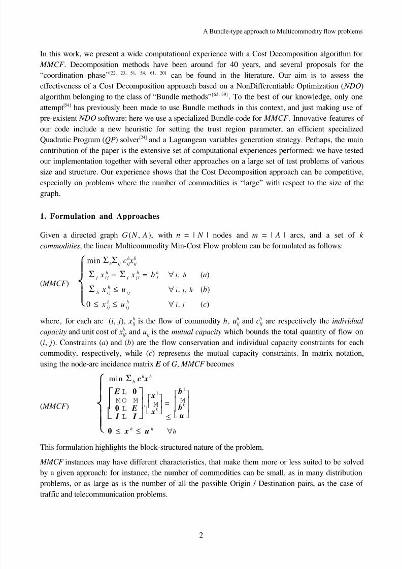
The m2 parameter, controlling the decrease of t , should be chosen “large” (≈ 3): the result is that t ischanged almost only in the early stages of the algorithm’s operations. Smaller values of m2 cause t todecrease too quickly, so yelding a very long sequence of “short” steps. This setting is remarkablydifferent from the one usually suggested in the literature, i.e. ≈ 0.9[47, 63]: the reason might be thatLagrangean functions of Linear Programs are qualitatively different from other classes of nondifferentiable functions, having an enormous number of facets which makes them extremely“kinky”. The choice of the other parameters is far less critical: m1 seems to be properly fixed to 0.1,
the (absolute and relative) safeguards on t almost never enter into play and the heuristics forincreasing and decreasing t are capable of correcting blatantly wrong initial estimates t 0. If t * has beenchosen sufficiently large, upon termination the current point λ is guaranteed to be an ε-optimalsolution of DMMCF : although selecting t * is in principle difficult, in practice it can be easily guessedby looking at a few test executions of the code.
An innovative feature of our code is the Lagrangean Variables Generation (LVG) strategy: rather thanalways working with the full vector of Lagrangean multipliers, we maintain a (hopefully small) set of “active” variables and only solve the restricted (Πβt ). Every p1 (≈ 10) iterations, we add to the activeset all “inactive” variables having the corresponding entry of d strictly positive; this is also done for
the first p2 (≈ 30) iterations, and when the algorithm would terminate because the STOP condition is

8/7/2019 A bundle type dual-ascent approach to linear multicommodity min-cost flow problems
http://slidepdf.com/reader/full/a-bundle-type-dual-ascent-approach-to-linear-multicommodity-min-cost-flow-problems 6/30
A Bundle-type approach to Multicommodity flow problems
6
verified. Usually, almost all the active variables reveal themselves in the first few iterations, and theactive set is very stable. Note that, from the primal viewpoint, the LVG strategy is a row generationscheme, where a complicating constraint is added only if it is violated by the primal unfeasiblesolution corresponding to d [16].
The LVG strategy has a dramatic impact on the time spent in solving (Πβt ), which is reduced by up toa factor of 5 even on small instances. Clearly, the LVG strategy can be beneficial only if the QP
solver efficiently supports the online creation and destruction of variables of subproblem (Πβt ): this is
the case of the specialized solver used in the code [24], which employs a two-level active set strategy forhandling the d ≥ − λ constraints. The availability of the specialized solver has been crucial fordeveloping an efficient Bundle code: other than supporting the LVG strategy, it is much faster thannon-specialized QP codes in solving sequences of (Πβt ) problems. This has been shown in [24] bycomparing it with two standard QP codes (interestingly enough, one of them being exactly the QP
solver used for the previous Bundle approach to MMCF [54]), which have been outperformed by up to
two orders of magnitude; since the coordination cost ranges from 1% to 20% of the total runningtime, a Bundle algorithm using a non-specialized QP solver would rapidly become impractical as theinstances size increases.
To keep the size of the Bundle low, we delete all the subgradients that have θi = 0 for more than afixed number (≈ 20) of consecutive iterations. We do not perform subgradients aggregation, since itusually has a negative impact on the total number of iterations.
In most cases, and especially if k is large, most of the time is spent in solving the MCF subproblems;hence, it is important to use a fast MCF solver with efficient reoptimizing capabilities. However, inmany classes of instances the MCF subproblems have a special structure that can be exploited: the
typical case is when all individual capacities uijh are either 0 or +∞ and there is only one source node
for each commodity, that is when the subproblems are Shortest Path Tree problems ( SPT ). In ourC++ code, Object-Oriented Programming techniques have been used to accomplish this: MCF
subproblems are solved with an implementation of the Relaxation algorithm[7], while SPT
subproblems are solved with classical Shortest Path algorithms[35]. Even on small problems with fewcommodities, this gives a speedup of up to four .
Object-Oriented Programming techniques have also been used in order to make it easy to developspecialized or extended versions. In fact, we already developed a parallel version of the code [14, 25], aswell as extended versions for computing lower bounds for the Fixed Charge MMCF [25, 15] and for theReserve Problem[25]. Only minor changes would be required for solving the Nonhomogeneous
MMCF , while the Nonlinear commodity-separable MMCF would only require the availability of asuitable nonlinear MCF solver.
Finally, we remark that, unlike other dual algorithms, our code is a “complete” MMCF solver, in thatupon termination it not only gives a dual optimal solution λ, but also a primal optimal solution
x = [ x1 ... x k ] = Σi∈β [ x i
1 ... x i
k ]θi
where x i
h is the solution of the h-th MCF with costs ch + λiand θ is the solution of the latest (∆βt
).Obtaining x requires keeping the flow solutions of the k MCF s relative to any subgradient in β, hence
it may considerably increase the memory requirements of the code; therefore, this feature has been

8/7/2019 A bundle type dual-ascent approach to linear multicommodity min-cost flow problems
http://slidepdf.com/reader/full/a-bundle-type-dual-ascent-approach-to-linear-multicommodity-min-cost-flow-problems 7/30
A. Frangioni and G. Gallo
7
made optional in the code, and in our experiments we have not used it. The impact on the runningtimes, however, is negligible (always well under 5%).
3. The other codes
One of the objectives of this research was to understand where a modern Cost Decomposition codestands, in terms of efficiency, among the solution methods proposed in the literature: hence, an efforthas been made to compare MMCFB with recent alternative MMCF solvers. The efficiency of CostDecomposition methods is controversial: although they have been used with success in someapplications, many researchers[37, 38] would agree that “... the folklore is that generally such schemestake a long time to converge so that they’re slower than just solving the model as a whole, althoughresearch continues. For now my advice, unless [...] your model is so huge that a good solver can’t fitit in memory, is to not bother decomposing it. It’s probably more cost effective to upgrade yoursolver, if the algorithm is limiting you ...”[27]. However, if Cost Decomposition approaches are of any
value, MMCF is probably the application where such a value shows up, as demonstrated by ourexperiments.
3.1 A general-purpose LP solver
In principle, any LP solver can be used to solve MMCF : actually, our experience shows that(according to above statement) commercial general-purpose LP solvers can be the best choice forsolving even quite large instances. This should not be surprising, since these codes are the result of an impressive amount of work and experience obtained during many years of development, andexploit the state of the art in matrix factorization algorithms, pricing rules, sophisticated data
structures, preprocessing and software technology. CPLEX 3.0[17] is one of the best commercial LP
solvers on the market: it offers Primal and Dual simplex algorithms, a Network simplex algorithm forexploiting the embedded network structure of the problems and a Barrier (Interior Point) algorithm.
Size PP PD HP HD
5 1 2 5 9 .02 2 .72 4 .73 1 .36
1 6 0 0 0 50 .90 23 .47 21 .37 6 .07
2 5 0 0 0 81 .05 14 .15 22 .65 5 .41
4 78 5 0 5 04 .0 4 1 24 .3 3 2 5. 48 1 0. 06
6 82 25 139 3.63 42 .24 18 .96 8 .10
6 1 2 7 5 1 6 4 6. 3 5 2 5 4 .1 3 1 8 5 .0 4 7 8 . 94
207733 16707 .66 492 .33 244 .89 44 .67257700 13301 .88 556 .39 165 .56 48 .55
Table 1: different simplex options for CPLEX
Size HD1 HD2 HD3 HD4
5 1 2 5 4 .08 1 .36 2 .11 1 .34
1 60 00 19 .65 5 .99 1 1.0 0 6 .0 8
2 50 00 18 .24 6 .16 1 9.7 1 5 .3 9
4 7 8 5 0 1 3 .3 5 1 1 .9 5 5 1 .0 3 1 0 .0 0
6 82 25 8 .05 1 0.76 7 1.5 9 8 .0 6
6 1 2 7 5 1 0 0 0 * 5 4 . 0 7 1 5 2 . 3 6 7 9 . 1 6
2 0 7 7 3 3 1 0 0 0 * 8 8 . 3 8 6 8 1 . 2 7 4 4 . 8 82 5 7 7 0 0 5 7 . 53 9 2 . 58 8 4 6 .6 5 4 8 .4 8
Table 2: different pricing rules for CPLEX
In our experimentation, to make the comparisons meaningful, efforts have been made to use CPLEXin its full power by repeatedly solving subsets of the test problems with different combinations of theoptimization parameters, in order to find a good setting. CPLEX can identify the network structureembedded in a LP, and efficiently solve the restricted problem to obtain a good starting base for the“Pure” Primal and Dual (PP and PD) simplex algorithms: the performances of the resulting “Hybrid”Primal and Dual algorithms (HP and HD) are reported in Table 1, where Size = mk is the number of
8/7/2019 A bundle type dual-ascent approach to linear multicommodity min-cost flow problems
http://slidepdf.com/reader/full/a-bundle-type-dual-ascent-approach-to-linear-multicommodity-min-cost-flow-problems 8/30
A Bundle-type approach to Multicommodity flow problems
8
variables of the LP and figures are the average running times over groups of several problems of thesame size. From these results, we see that a Dual approach can be 30 times faster than a Primal one,and that the “warm start” speeds up the solution by up to a factor of 70, so that the Hybrid Dualversion can be 400 times faster than the Pure Primal one. Hence, it is not unfair to regard CPLEX as
a semi-specialized algorithm for network-structured problems. Other details, such as the pricingstrategy, can have a dramatic impact on the number of iterations and hence on the performance: Table2 reports a comparison between the four available pricing rules for the Dual simplex, the standarddual pricing HD1 and three variants of the steepest-edge rule HD2-4. Performance improvements of up to a factor of 15 (and more, since the instances marked with “*” had taken much longer than 1000seconds to terminate) can be obtained by selecting the appropriate rule.
3.2 A Primal Partitioning code
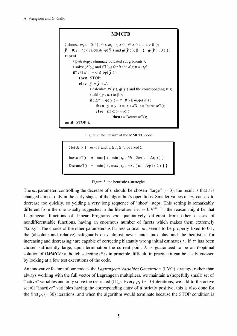
PPRN 1.0[12] is an available (in .a format at ftp://ftp-eio.upc.es/pub/onl/codes/pprn/libpprn) recent
implementation of the Reduced Gradient algorithm for theNonlinear MMCF , i.e. a Primal Partitioning approach whenapplied to the linear case. In their computational experience[18], theauthors show that it generally outperforms the known PrimalPartitioning code MCNF85[46]. In our experience, PPRN hasnever shown to be dramatically faster then CPLEX: however, thisshould not lead to the conclusion that it is inefficient. In fact,PPRN is a primal code, and it is definitely much faster than theprimal simplex of CPLEX: hence, it can be regarded as a good
representative of its class of methods.Again, an appropriate tuning of its (several) parameters cansignificantly enhance the performances. The most importantchoice concerns the Phase 0 strategy, i.e. whether the startingbase is obtained from any feasible solution of the k MCF
subproblems rather than from their optimal solutions (as in the“warm start” of CPLEX). As shown in Table 3, exploiting theoptimal solutions decreases the running times by up to a factor of 20 (Opt vs. Feas columns): moreover, appropriate selection of the
pricing rule[12]
can result in a speedup of 3, as shown in Table 4.
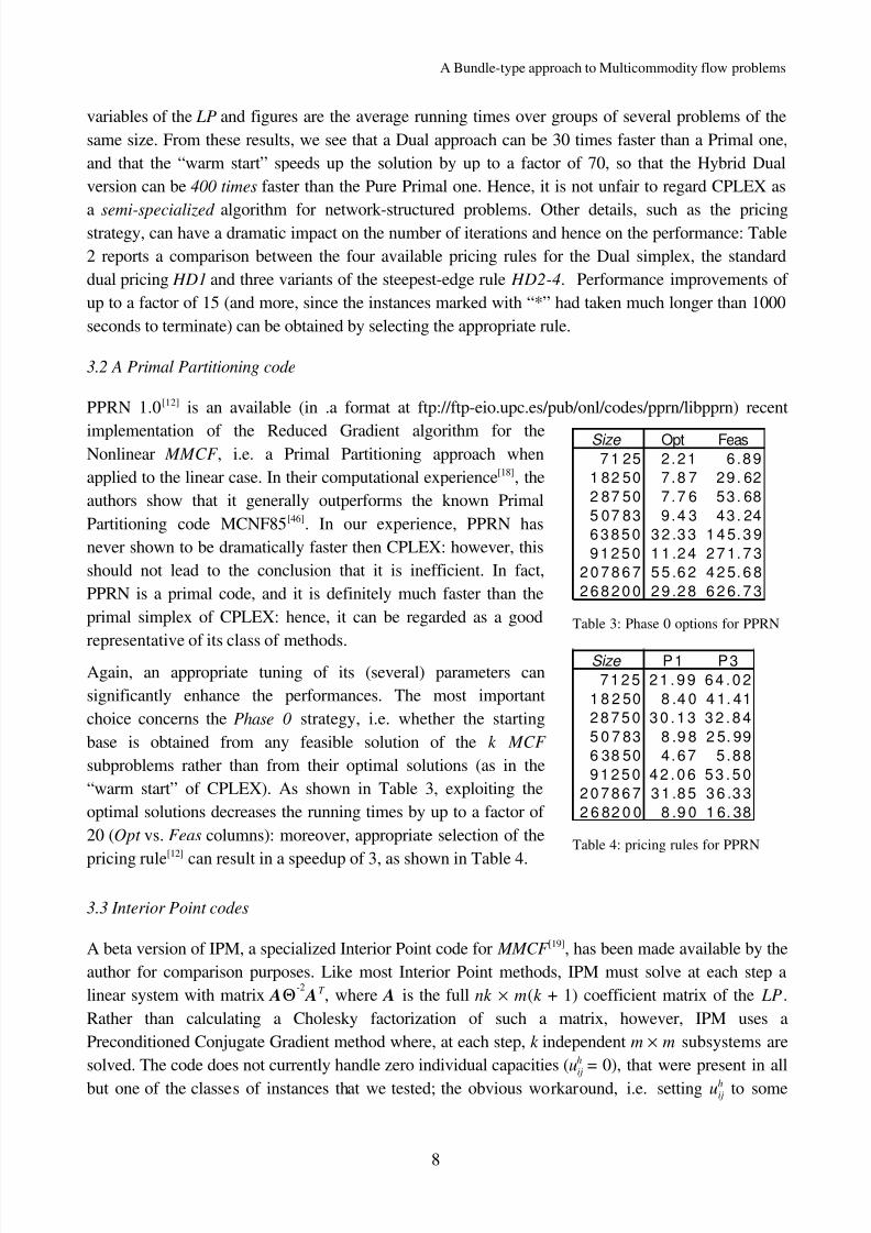
3.3 Interior Point codes
A beta version of IPM, a specialized Interior Point code for MMCF [19], has been made available by theauthor for comparison purposes. Like most Interior Point methods, IPM must solve at each step alinear system with matrix AΘ
-2AT , where A is the full nk × m(k + 1) coefficient matrix of the LP.
Rather than calculating a Cholesky factorization of such a matrix, however, IPM uses aPreconditioned Conjugate Gradient method where, at each step, k independent m × m subsystems aresolved. The code does not currently handle zero individual capacities (uij
h = 0), that were present in all
but one of the classes of instances that we tested; the obvious workaround, i.e. setting uijh to some
Size Opt Feas
7 1 25 2 .21 6 .89
1 82 50 7 .8 7 29. 62
2 87 50 7 .7 6 53. 68
5 07 83 9 .4 3 43. 24
6 3 8 5 0 3 2 .3 3 1 4 5. 3 9
9 1 2 5 0 1 1 .2 4 2 7 1. 7 3
2 0 7 8 6 7 5 5 .6 2 4 2 5. 6 8
2 6 8 2 0 0 2 9 .2 8 6 2 6. 7 3
Table 3: Phase 0 options for PPRN
Size P1 P3
7 1 2 5 2 1 . 9 9 6 4 . 0 2
1 8 2 50 8 .4 0 4 1. 41
2 8 7 5 0 3 0 . 1 3 3 2 . 8 4
5 0 7 83 8 .9 8 2 5. 99
6 38 50 4 .67 5 .88
9 1 2 5 0 4 2 . 0 6 5 3 . 5 0
2 0 7 8 6 7 3 1 .8 5 3 6 .3 3
2 6 82 0 0 8 .9 0 1 6. 38
Table 4: pricing rules for PPRN
8/7/2019 A bundle type dual-ascent approach to linear multicommodity min-cost flow problems
http://slidepdf.com/reader/full/a-bundle-type-dual-ascent-approach-to-linear-multicommodity-min-cost-flow-problems 9/30
A. Frangioni and G. Gallo
9
very small number and/or cij
h to some very large number, might result in numerical problems, yet thecode was able to solve (almost) all the instances.
Since only indirect comparisons were possible for the other specialized Interior Point methods (Cf.§3.5), we also tested two general-purpose Interior Point LP solvers: CPLEX 3.0 Barrier (that will be
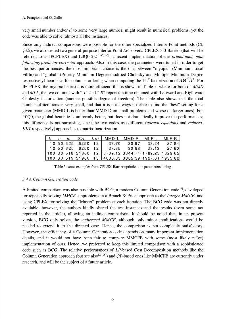
referred to as IPCPLEX) and L0Q0 2.21 [66, 65], a recent implementation of the primal-dual, pathfollowing, predictor-corrector approach. Also in this case, the parameters were tuned in order to getthe best performances: the most important choice is the one between “myopic” (Minimum LocalFillIn) and “global” (Priority Minimum Degree modified Cholesky and Multiple Minimum Degreerespectively) heuristics for columns ordering when computing the LLT factorization of AΘ
−2AT . For
IPCPLEX, the myopic heuristic is more efficient; this is shown in Table 5, where for both of MMD
and MLF , the two columns with “-L” and “-R” report the time obtained with Leftward and RightwardCholesky factorization (another possible degree of freedom). The table also shows that the totalnumber of iterations is very small, and that it is not always possible to find the “best” setting for a
given parameter (MMD-L is better than MMD-D on small problems and worse on larger ones). ForL0Q0, the global heuristic is uniformly better, but does not dramatically improve the performances;this difference is not surprising, since the two codes use different (normal equations and reduced-
KKT respectively) approaches to matrix factorization.
k n m Size I t e r MMD- L MMD-R ML F- L MLF-R
1 0 5 0 6 25 6 2 5 0 1 2 37.70 30 .97 33 .24 27.84
1 0 5 0 6 25 6 2 5 0 1 2 37.35 30 .98 33 .13 27.60
1 0 0 3 0 5 1 8 5 1 8 0 0 1 2 3 70 9 .1 2 3 3 4 4. 74 1 7 89 .2 3 1 8 2 9. 6 5
1 0 0 3 0 5 1 9 5 1 9 0 0 1 3 4 03 6 .8 3 3 3 8 2. 39 1 9 27 .0 1 1 9 3 5. 8 2
Table 5: some examples from CPLEX-Barrier optimization parameters tuning
3.4 A Column Generation code
A limited comparison was also possible with BCG, a modern Column Generation code [9], developedfor repeatedly solving MMCF subproblems in a Branch & Price approach to the Integer MMCF , andusing CPLEX for solving the “Master” problem at each iteration. The BCG code was not directlyavailable; however, the authors kindly shared the test instances and the results (even some notreported in the article), allowing an indirect comparison. It should be noted that, in its presentversion, BCG only solves the undirected MMCF , although only minor modifications would be
needed to extend it to the directed case. Hence, the comparison is not completely satisfactory.However, the efficiency of a Column Generation code depends on many important implementationdetails, and it would not have been fair to compare MMCFB with some (most likely naïve)implementation of ours. Hence, we preferred to keep this limited comparison with a sophisticatedcode such as BCG. The relative performances of LP-based Cost Decomposition methods like theColumn Generation approach (but see also[25, 26]) and QP-based ones like MMCFB are currently underresearch, and will be the subject of a future article.
8/7/2019 A bundle type dual-ascent approach to linear multicommodity min-cost flow problems
http://slidepdf.com/reader/full/a-bundle-type-dual-ascent-approach-to-linear-multicommodity-min-cost-flow-problems 10/30
A Bundle-type approach to Multicommodity flow problems
10
3.5 Other codes
The above codes do not exhaust all the proposed computational approaches to MMCF : indirectcomparison have been made also with other Interior Point methods[70, 62], different CostDecomposition approaches[61, 69] and ε-approximation algorithms[33]. The comparison concerns thePDS problems (Cf. §4.3), that are difficult MMCF s with large graphs but few commodities and MCF
subproblems: hence, the results do not necessarily provide useful information on other classes of instances, such as those arising in telecommunications, which are characterized by a large number of commodities. Furthermore, the codes were ran on a heterogeneous set of computers, ranging from(vector or massively parallel) supercomputers to (clusters of) workstations, making it difficult toextract meaningful information from the running times reported.
No comparison at all was possible with Resource Decomposition approaches[49] or Primal-Dualmethods[67]: however, the available codes are at least sufficient to draw an initial picture of the currentscenery of computational approaches to MMCF . Hopefully, other tests will come to further enhanceour understanding.
4. The test problems
The other fundamental ingredient for obtaining a meaningful computational comparison is an adequateset of test problems. Some data sets and random generators of MMCF s have been used in theliterature to test some of the proposed approaches: however, many of these test problems are small,and even the larger ones have a small number of commodities. This is probably due to the fact that,with most of the methods, the cost for solving an MMCF grows rapidly with k , so that problems with
hundreds of commodities have for long time been out of reach. For our experiments, some knowndata sets have been gathered that might be considered representative of classes of instances arising inpractice: when no satisfactory test problems were available, different random generators have beenused to produce data sets with controlled characteristics. All these instances, and some others, can beretrieved at http://www.di.unipi.it/di/groups/optimize/Data/MMCF.html together with an instance-by-instance output for all the codes listed in §3. We hope that this database will grow and will form thebasis for more accurate computational comparisons in the future.
4.1 The Canad problems
The first data set is made of 96 problems, generated with two random generators (one for bipartiteand the other for general graphs) developed to test algorithms for the Fixed Charge MMCF
problem[15]. A parameter, called capacity ratio, is available as a “knob” to produce lightly or heavilycapacitated instances. As MMCF s, these instances have proven a posteriori to be quite “easy”; on thecontrary, the corresponding Fixed Charge problems are known to be “hard”, and hence the efficientsolution of “easy” MMCF s can still have an interest. Furthermore, this data set is the only one havinginstances where the number of commodities is considerably larger that the number of nodes (up to400 vs. 30), as in some real applications. The instances are divided into the three groups:
− 32 bipartite problems (group A) with multiple sources and sinks for each commodity;
8/7/2019 A bundle type dual-ascent approach to linear multicommodity min-cost flow problems
http://slidepdf.com/reader/full/a-bundle-type-dual-ascent-approach-to-linear-multicommodity-min-cost-flow-problems 11/30
A. Frangioni and G. Gallo
11
− 32 nonbipartite problems (group B) with single source/sink for each commodity;
− 32 nonbipartite problems (group C) with multiple sources and sinks for each commodity.
The characteristics of the instances are shown in Table 6 (§5.1): for each choice of (k , n, m), two“easy” and two “hard” instances have been generated.
4.2 The Mnetgen generator
Mnetgen[1] is a well-known random generator. An improved version has been developed for our tests,where the internal random number generator has been replaced with the standard drand48()
routine, the output file format has been “standardized”[41] and a minor bug has been fixed. 216problems have been generated with the following rules: the problems are divided in 18 groups of 12problems each, each group being characterized by a pair (n, k ) for n in {64, 128, 256} and k in {4,8, ... , n} (as Mnetgen cannot generate problems with k > n). Within each group, 6 problems are
“sparse” and 6 are “dense”, with m / n respectively equal to about 3 and 8. In both these subgroups, 3problems are “easy” and 3 are “hard”, where an easy problem has mutual capacity constraints on 40%of the arcs and 10% of the arcs with an “high” cost, while these figures are 80% and 30%respectively for a hard problem. Finally, the 3 subproblems characterized by the 4-tuple ( n, k , S , D)(S ∈ {sparse, dense}, D ∈ {easy, hard}) have respectively 30%, 60% and 90% of arcs withindividual capacity constraints. Randomly generated instances are believed to be generally “easier”than real-world problems; however, the “hard” Mnetgen instances, especially if “dense”, have provento be significantly harder to solve (by all the codes) than both the “easy” ones and instances of equivalent size taken from the other sets of test problems.
4.3 The PDS problems
The PDS (Patient Distribution System) instances derive from the problem of evacuating patients froma place of military conflict. The available data represents only one basic problem, but the model isparametric in the planning horizon t (the number of days): the problems have a time-space networkwhose size grows about linearly with t . This characteristic is often encountered in MMCF models of transportation and logistic problems. However, in other types of applications k also grows with theplanning horizon, while in the PDS problems k is a constant (11); hence, the larger instances have avery large m / k ratio.
4.4 The JLF data set
This set of problems has been used in [42] to test the DW approach to MMCF : it contains various(small) groups of small real-world problems with different structures, often with SPT subproblemsand with never more than 15 commodities.
4.5 The dimacs2pprn “meta” generator
Several MMCF s, especially those arising in telecommunications, have large graphs, manycommodities and SPT subproblems; all these characteristics are separately present in some of the
previous data sets, but never in the same instance. To generate such instances, we developed a

8/7/2019 A bundle type dual-ascent approach to linear multicommodity min-cost flow problems
http://slidepdf.com/reader/full/a-bundle-type-dual-ascent-approach-to-linear-multicommodity-min-cost-flow-problems 12/30
A Bundle-type approach to Multicommodity flow problems
12
slightly enhanced version of the dimacs2pprn “meta” generator, originally proposed in [18], that allowsa great degree of freedom in the choice of the problem structure. Dimacs2pprn inputs an MCF inDIMACS standard format (ftp://dimacs.rutgers.edu/pub/netflow), i.e. a graph G with arc costs c,node deficits b , arc capacities u and three parameters k , r and f , and constructs an MMCF with k
commodities on the same graph G¯
. Deficits and capacities of the i-th subproblem are a “scaling” of those of the original MCF , i.e. k numbers { r 1 .. r k } are uniformly drawn at random from [ 1 .. r ]and the deficits and individual capacities are chosen as bh = r hb and uh = r hu; costs cij
h areindependently and uniformly drawn randomly from [ 0 .. cij ]. The mutual capacities u are initiallyfixed to f u, and eventually increased to accommodate the multiflow obtained by solving the k MCF sseparately (with random costs uncorrelated with the cij
h), in order to ensure the feasibility of theinstance. At the user’s choice, the individual capacities can then be set to +∞. This is a “meta”generator since most of the structure of the resulting MMCF is not “hard-wired” into the generator,like in Mnetgen, but depends on the initial MCF ; in turn, this initial MCF can be obtained with arandom generator. For our tests, we used the well-known Rmfgen [29], which, given two integervalues a and b, produces a graph made of b squared grids of side a, with one source and one sink atthe “far ends” of the graph. For all 6 combinations of a in {4, 8} and b in {4, 8, 16}, an “easy” and a“hard” MCF have been generated with maximum arc capacities respectively equal to 1/2 and 1/10 of the total flow to be shipped. Then, for each of these 12 MCF s, 4 MMCF s have been generated, withk in {4, 16, 64, 256}, r = 16 and f = 2k (so that the mutual capacity constraints were four times“stricter” than the original capacities u), yielding a total of 48 instances with up to one million of variables.
4.6 The BHV problems
Two sets of randomly generated undirected MMCF s have been used to test the Column Generationapproach of [9]. In both sets, the commodities are intended to be Origin / Destination pairs, but thecommodities with the same origin can be aggregated in a much smaller number of single origin -many destinations flows. The 12 “qx” problems all have 50 nodes, 130 arcs (of which 96 arecapacitated) and 585 O/D pairs that can be aggregated into 48 commodities, yielding a total LP size of 6.2.103; a posteriori, they have proven to be quite easy. The 10 “r10-x-y” problems all have 301nodes, 497 arcs (of which 297 are capacitated) and 1320 O/D pairs that can be aggregated into 270commodities, yelding a total LP size of 1.3.105. The group is divided into 5 “r10-5-y” and 5 “r10-55-y” instances that are similar, but for the fact that the arc capacities in the first group are integral while
those in the second one are highly fractional: the two subgroups have proven to be of a surprisinglydifferent “difficulty”.
5. Computational results and conclusions
In this paragraph, we report on the comparison of MMCFB with the codes described in §3 on the testproblems described in §4. The approaches being very different, it appears that the only performancemeasure which allows a meaningful comparison is the running time. In the following, we report CPUtime in seconds needed to solve the different problems; the loading and preprocessing times have not
been included. Information like the number of iterations (with different meanings for each code) or

8/7/2019 A bundle type dual-ascent approach to linear multicommodity min-cost flow problems
http://slidepdf.com/reader/full/a-bundle-type-dual-ascent-approach-to-linear-multicommodity-min-cost-flow-problems 13/30
A. Frangioni and G. Gallo
13
the time spent in different parts of the optimization process (e.g. for computing ϕ and solving (∆βt ))
has not been reported in the tables for reasons of space and clarity: all these data are however availableat the above mentioned Web page.
Unless explicitly stated, the times have been obtained on a HP9000/712-80 workstation: for the codes
run on different machines, the original figures will be reported and a qualitative estimate of the relativespeed has been obtained—if possible—by comparing the SPECint92 and SPECfp92 figures (97.1and 123.3 respectively for the HP9000/712-80). For MMCFB, CPLEX (both simplex and InteriorPoint) and L0Q0, the required relative precision was set to 10 -6: in fact, the reported values of theoptimal solution always agree in the first 6 digits. PPRN do not allow such a choice, but it alwaysobtained solutions at least as accurate as the previous codes. Upon suggestion of the authors, therelative precision required for IPM was instead set to 10 -5, as smaller values could cause numericaldifficulties to the PCG: in fact, the values obtained were often different in the sixth digit. Theprecision of the BCG code is not known to us, but should be comparable: the other codes will be
explicitly discussed later.In all the following tables, b (< m), if present, is the number of arcs that have a mutual capacityconstraint, and, for large data sets, each entry is averaged from a set of instances with similarsize = mk . The columns with the name of a code contain the relative running time; “*” means thatsome of the the instances of that group could not be solved due to memory problems, “**” means thatthe code aborted due to numerical problems and “***” indicates that the computation had to beinterrupted because the workstation was “thrashing”, i.e. spending almost all the time in pagingvirtual memory faults.
5.1 The Canad problems
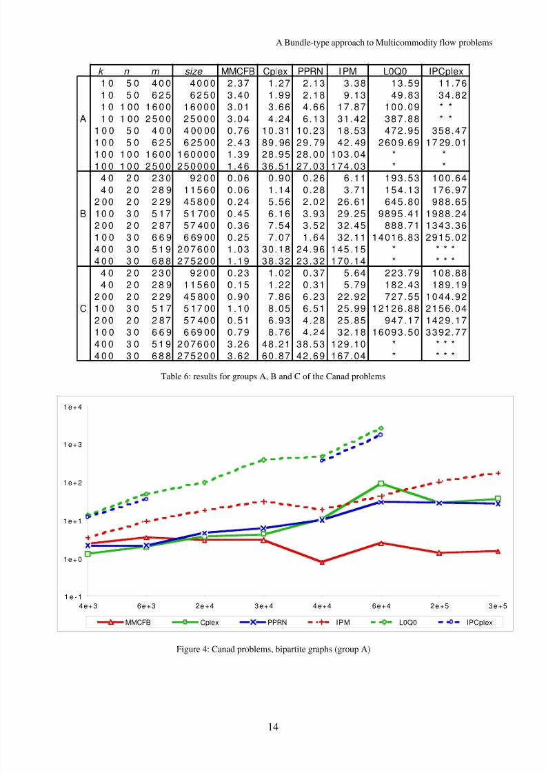
The results of the three groups of instances A, B and C are summarized in Table 6: they are alsovisualized in Figure 4, Figure 5 and Figure 6 for the three groups separately, where the running timeof each algorithm is plotted as a function of the size.
If compared to the faster code, the general-purpose Interior Point solvers are 2 to 3 orders of magnitude slower on groups B and C and 1 to 2 on group A; furthermore, they were not able to solvethe largest instances due to memory or numerical problems. The specialized IPM is (approximately) 3to 20 times faster on group A, 20 to 70 times faster on group B and 10 to 40 times faster on group C:however, it is almost never competitive with any of MMCFB, CPLEX and PPRN. Among thoselatter solvers, MMCFB is 10 to 40 times faster than CPLEX and 5 to 20 times faster than PPRN onall instances; an exception is the first half of group A, where MMCFB is less than 2 times slower.These are “difficult” small instances with few commodities, where MMCFB requires considerablymore ϕ evaluations than for all the other problems. This may lead to the conjecture that MMCFB isnot competitive on “difficult” instances, but the following experiences will show that this is true onlyif the number of commodities is also small.
8/7/2019 A bundle type dual-ascent approach to linear multicommodity min-cost flow problems
http://slidepdf.com/reader/full/a-bundle-type-dual-ascent-approach-to-linear-multicommodity-min-cost-flow-problems 14/30
A Bundle-type approach to Multicommodity flow problems
14
k n m size MMCFB Cplex PPRN I PM L0Q0 IPCplex
1 0 5 0 4 0 0 4 0 0 0 2 .37 1 .27 2 .13 3 .38 13 .59 11.76
1 0 5 0 6 2 5 6 2 5 0 3 .40 1 .99 2 .18 9 .13 49 .83 34.82
1 0 1 00 1 6 0 0 1 6 0 0 0 3 .01 3 .66 4 .66 17.87 100.09 * *
A 1 0 1 00 2 5 0 0 2 5 0 0 0 3 .04 4 .24 6 .13 31.42 387.88 * *
1 0 0 5 0 4 0 0 4 00 00 0 .76 10.31 10.23 18.53 472.95 358.471 0 0 5 0 6 2 5 6 25 00 2 .4 3 89. 96 29. 79 42. 49 260 9.69 17 29.01
1 0 0 1 0 0 1 6 0 0 1 6 0 00 0 1 .39 28.95 28.00 103 .04 * *
1 0 0 1 0 0 2 5 0 0 2 5 0 00 0 1 .46 36.51 27.03 174 .03 * *
4 0 2 0 2 3 0 9 2 0 0 0 .06 0 .90 0 .26 6 .11 193.53 100.64
4 0 2 0 2 8 9 1 1 5 6 0 0 .06 1 .14 0 .28 3 .71 154.13 176.97
2 00 2 0 2 29 4 5 8 0 0 0 .24 5 .56 2 .02 26.61 645.80 988.65
B 10 0 3 0 5 17 5 1 70 0 0 .45 6 .16 3 .93 29.25 9895.41 1988.24
2 00 2 0 2 87 5 7 40 0 0 .36 7 .54 3 .52 32.45 888.71 1343.36
1 0 0 3 0 6 6 9 6 69 00 0 .25 7 .07 1 .64 32.11 14016.83 2915.02
4 0 0 3 0 5 1 9 2 0 7 60 0 1 .03 30.18 24.96 145 .15 * * * *
4 0 0 3 0 6 8 8 2 7 5 20 0 1 .19 38.32 23.32 170 .14 * * * *
4 0 2 0 2 3 0 9 2 0 0 0 .23 1 .02 0 .37 5 .64 223.79 108.884 0 2 0 2 8 9 1 1 5 6 0 0 .15 1 .22 0 .31 5 .79 182.43 189.19
2 00 2 0 2 29 4 5 80 0 0 .90 7 .86 6 .23 22.92 727.55 1044.92
C 1 0 0 3 0 5 1 7 5 17 00 1 .10 8 .05 6 .51 25.99 12126.88 2156.04
2 00 2 0 2 87 5 7 40 0 0 .51 6 .93 4 .28 25.85 947.17 1429.17
1 0 0 3 0 6 6 9 6 69 00 0 .79 8 .76 4 .24 32.18 16093.50 3392.77
4 0 0 3 0 5 1 9 2 0 7 60 0 3 .26 48.21 38.53 129 .10 * * * *
4 0 0 3 0 6 8 8 2 7 5 20 0 3 .62 60.87 42.69 167 .04 * * * *
Table 6: results for groups A, B and C of the Canad problems
1 e - 1
1 e + 0
1 e + 1
1 e + 2
1 e + 3
1 e + 4
4 e + 3 6 e + 3 2 e + 4 3 e + 4 4 e + 4 6 e + 4 2 e + 5 3 e + 5
MMCFB Cplex PPRN IPM L0Q0 IPCplex
Figure 4: Canad problems, bipartite graphs (group A)

8/7/2019 A bundle type dual-ascent approach to linear multicommodity min-cost flow problems
http://slidepdf.com/reader/full/a-bundle-type-dual-ascent-approach-to-linear-multicommodity-min-cost-flow-problems 15/30
A. Frangioni and G. Gallo
15
1 e - 2
1 e - 1
1 e + 0
1 e + 1
1 e + 2
1 e + 3
1 e + 4
1 e + 5
9 e + 3 1 e + 4 5 e + 4 5 e + 4 6 e + 4 7 e + 4 2 e + 5 3 e + 5
MMCFB Cplex PPRN IPM L0Q0 IPCplex
Figure 5: Canad problems, generic graphs (group B)
1 e - 1
1 e + 0
1 e + 1
1 e + 2
1 e + 3
1 e + 4
1 e + 5
9 e + 3 1 e + 4 5 e + 4 5 e + 4 6 e + 4 7 e + 4 2 e + 5 3 e + 5
MMCFB Cplex PPRN IPM L0Q0 IPCplex
Figure 6: Canad problems, generic graphs (group C)
5.2 The Mnetgen problems
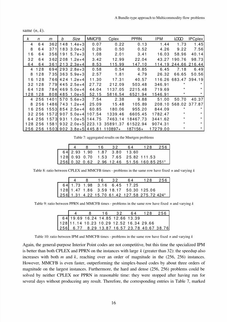
The Mnetgen problems have a wide range of different characteristics, from small to very large sizes(more than 5.105 variables), and from small to very large m / k ratios. Table 7 and Figure 7
summarize the results we have obtained; the times are the averages taken over 12 problems with the
8/7/2019 A bundle type dual-ascent approach to linear multicommodity min-cost flow problems
http://slidepdf.com/reader/full/a-bundle-type-dual-ascent-approach-to-linear-multicommodity-min-cost-flow-problems 16/30
A Bundle-type approach to Multicommodity flow problems
16
same (n, k ).
k n m b Size MMCFB Cplex PPRN IPM LOQO IPCplex
4 6 4 36 2 1 4 8 1.4e+3 0 .07 0 .22 0 .13 1 .44 1 .73 1 .45
8 6 4 37 1 1 8 3 3.0e+3 0 .26 0 .50 0 .52 4 .26 9 .22 7 .56
1 6 6 4 3 5 6 1 9 1 5.7e+3 1 .08 2 .01 3 .41 16 .03 58 .96 40 .14
3 2 6 4 3 62 2 08 1.2e+4 3 .42 12 .99 22.04 43 .27 190 .76 98 .73
6 4 6 4 3 6 1 2 1 3 2.3e+4 8 .53 115 .99 147.10 114 .19 244 .66 216.44
4 1 2 8 6 9 4 2 9 3 2.8e+3 0 .58 0 .54 0 .85 6 .45 7 .18 6 .49
8 1 2 8 7 3 5 3 6 3 5.9e+3 2 .57 1 .81 4 .79 26 .32 6 6 .65 5 0 .56
1 6 1 2 8 7 6 6 4 2 4 1.2e+4 11 .30 17 .31 40.57 116 .26 683 .47 394.19
3 2 1 2 8 7 7 9 4 4 5 2.5e+4 2 7 .72 212 .09 503.48 346 .91 * *
6 4 1 2 8 7 8 4 4 6 9 5.0e+4 44 .04 1137 .05 2215.48 719 .69 * *
1 2 8 1 2 8 8 0 8 4 8 5 1.0e+5 52 .15 5816 .54 6521.94 1546 .91 * *
4 2 5 6 1 4 0 1 5 7 0 5.6e+3 7 .54 2 .38 9 .88 51 .00 50 .70 40 .37
8 2 5 6 1 48 6 7 4 3 1.2e+4 25 .09 15 .48 105. 89 208 .10 568 .02 37 7.87
1 6 2 5 6 1 5 5 3 8 5 4 2.5e+4 60 .85 180 .06 955.20 844 .09 * *
3 2 2 56 1 5 7 2 9 07 5.0e+4 107.54 1339 .46 6605.45 1782 .47 * *6 4 2 56 1 57 3 9 3 1 1.0e+5 144.75 7463 .14 18467 .73 3441 .62 * *
1 28 2 56 1 58 1 9 3 2 2.0e+5 223.13 35891.37 61522 .94 9074 .31 * *
2 5 6 2 5 6 1 5 0 3 9 0 2 3.8e+5 4 45 .8 1 110897+ 187156+ 1 72 79 .0 0 * *
Table 7: aggregated results on the Mnetgen problems
4 8 1 6 3 2 6 4 1 2 8 2 5 6
6 4 2. 93 1. 90 1 .8 7 3 .8 0 1 3. 60
1 2 8 0. 93 0. 70 1 .5 3 7 .6 5 2 5. 82 1 11 .5 3
2 5 6 0 . 32 0 . 6 2 2 . 96 1 2. 4 6 5 1 .5 6 1 6 0. 8 5 251*
Table 8: ratio between CPLEX and MMCFB times - problems in the same row have fixed n and varying k
4 8 1 6 3 2 6 4 1 2 8 2 5 6
6 4 1. 73 1. 98 3 .1 6 6 .4 5 1 7. 25
1 2 8 1 . 47 1 .8 6 3 .5 9 1 8. 17 5 0. 30 1 25 .0 6
25 6 1 .31 4 .22 15 .70 61 .42 127 .58 275 .72 424*
Table 9: ratio between PPRN and MMCFB times - problems in the same row have fixed n and varying k
4 8 1 6 3 2 6 4 1 2 8 2 5 6
6 4 19 .69 16 .24 14 .85 12 .66 13 .39
1 2 8 1 1 . 1 4 1 0 . 2 3 1 0 . 2 9 1 2 . 5 2 1 6 . 3 4 2 9 . 6 6
2 5 6 6 .7 7 8 .2 9 1 3. 8 7 1 6. 5 7 2 3. 7 8 4 0. 6 7 3 8. 7 6
Table 10: ratio between IPM and MMCFB times - problems in the same row have fixed n and varying k
Again, the general-purpose Interior Point codes are not competitive, but this time the specialized IPMis better than both CPLEX and PPRN on the instances with large k (greater than 32): the speedup alsoincreases with both m and k , reaching over an order of magnitude in the (256, 256) instances.However, MMCFB is even faster, outperforming the simplex-based codes by about three orders of magnitude on the largest instances. Furthermore, the hard and dense (256, 256) problems could besolved by neither CPLEX nor PPRN in reasonable time: they were stopped after having run for
several days without produceing any result. Therefore, the corresponding entries in Table 7, marked

8/7/2019 A bundle type dual-ascent approach to linear multicommodity min-cost flow problems
http://slidepdf.com/reader/full/a-bundle-type-dual-ascent-approach-to-linear-multicommodity-min-cost-flow-problems 17/30
A. Frangioni and G. Gallo
17
with a “+”, are actually (mild) estimates.
1e-1
1e+0
1e+1
1e+2
1e+3
1e+4
1e+5
( 4, 6
4)
( 8, 6
4)
( 16,
64)
( 32,
64)
( 64,
64)
( 4, 1
28)
( 8, 1
28)
( 16,
128)
( 321
28)
( 64,
128)
( 128
, 128
)
( 4, 2
56)
( 8, 2
56)
( 16,
256)
( 32,
256)
( 64,
256)
( 128
, 256
)
( 256
, 256
)
MMCFB Cplex PPRN IPM LOQO IPCplex
Figure 7: aggregated results on the Mnetgen problems
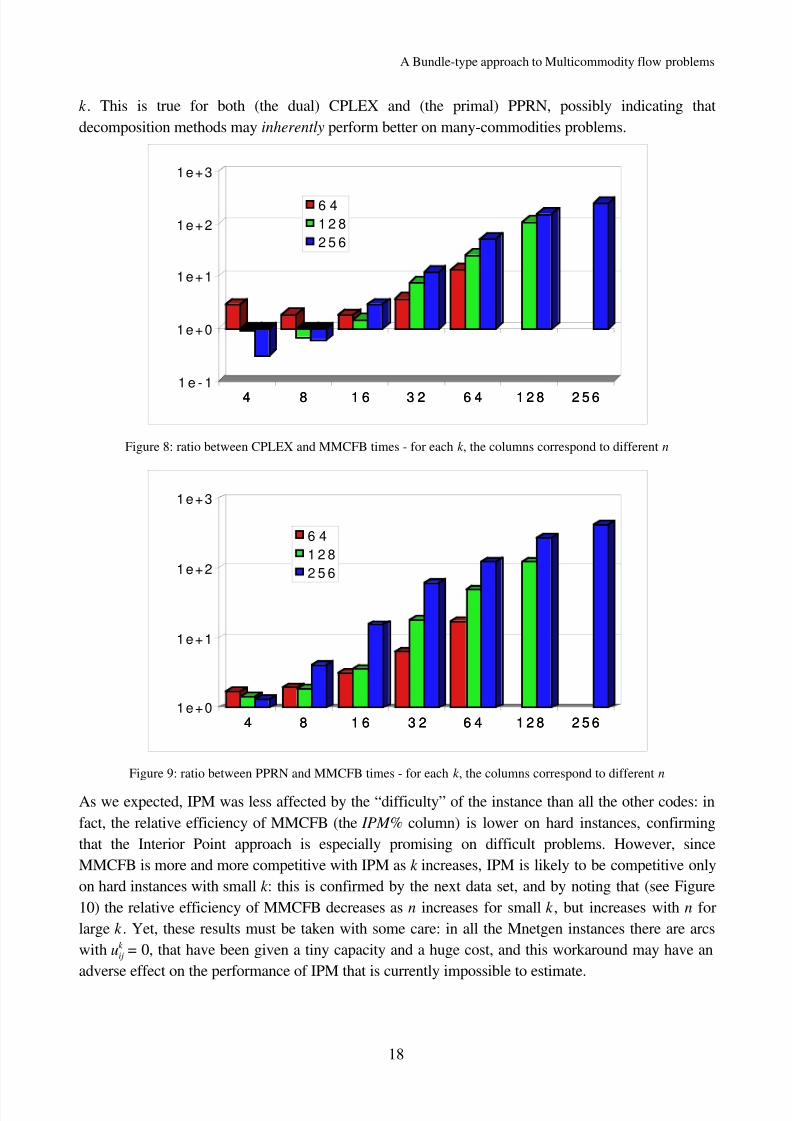
However, a closer examination of the results enlightens the weakness of MMCFB on large instanceswith few commodities. This is better seen in Table 8, Table 9 and Table 10, and the correspondingFigure 8, Figure 9 and Figure 10, where the ratio between the running times of CPLEX (respectivelyPPRN and IPM) and MMCFB is reported for different values of (n, k )—the entries marked with a“*” are those based on estimates, and should actually be larger. MMCFB is slower than CPLEX byup to a factor of 4 for instances with a large m / k ratio: more disaggregated data about some “critical”
256-nodes problems are reported in Table 11 for a better understanding of the phenomenon.Noticeably, “hard” problems (h) are really harder to solve, for all the codes, than “easy” ones (e) of the same size; moreover, they are much harder than, e.g., Canad problems of comparable size, sincea 1.6.105 variables (100, 100, 1600) Canad instance can be solved in 1.5 seconds, while a hard1.5.105 variables (64, 256, 2300) Mnetgen instance requires over 350 seconds.On problems with few commodities, MMCFB is about 2 times slower than CPLEX when theinstances are easy, and about 4 times slower in the case of hard ones. Conversely, as the number of commodities increases, the relative efficiency (the Cplex% and PPRN% columns) of MMCFB islarger on hard instances than on easy ones, and it increases with the problem size. This is probablydue to the fact that the number of ϕ evaluations depends on the “hardness” of the instance, but much
less on k , while the number of simplex iterations tends to increase under the combined effect of m and
8/7/2019 A bundle type dual-ascent approach to linear multicommodity min-cost flow problems
http://slidepdf.com/reader/full/a-bundle-type-dual-ascent-approach-to-linear-multicommodity-min-cost-flow-problems 18/30
A Bundle-type approach to Multicommodity flow problems
18
k . This is true for both (the dual) CPLEX and (the primal) PPRN, possibly indicating thatdecomposition methods may inherently perform better on many-commodities problems.
4 8 1 6 3 2 6 4 1 2 8 2 5 61 e - 1
1e+0
1e+1
1e+2
1e+3
4 8 1 6 3 2 6 4 1 2 8 2 5 6
6 4
1 2 8
2 5 6
Figure 8: ratio between CPLEX and MMCFB times - for each k , the columns correspond to different n
4 8 1 6 3 2 6 4 1 2 8 2 5 61e+0
1e+1
1e+2
1e+3
4 8 1 6 3 2 6 4 1 2 8 2 5 6
6 4
1 2 8
2 5 6
Figure 9: ratio between PPRN and MMCFB times - for each k , the columns correspond to different n
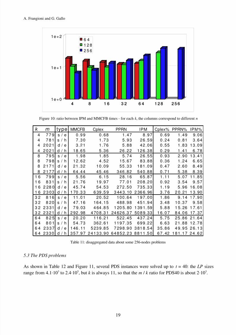
As we expected, IPM was less affected by the “difficulty” of the instance than all the other codes: infact, the relative efficiency of MMCFB (the IPM% column) is lower on hard instances, confirmingthat the Interior Point approach is especially promising on difficult problems. However, sinceMMCFB is more and more competitive with IPM as k increases, IPM is likely to be competitive onlyon hard instances with small k : this is confirmed by the next data set, and by noting that (see Figure10) the relative efficiency of MMCFB decreases as n increases for small k , but increases with n forlarge k . Yet, these results must be taken with some care: in all the Mnetgen instances there are arcswith uij
k = 0, that have been given a tiny capacity and a huge cost, and this workaround may have anadverse effect on the performance of IPM that is currently impossible to estimate.
8/7/2019 A bundle type dual-ascent approach to linear multicommodity min-cost flow problems
http://slidepdf.com/reader/full/a-bundle-type-dual-ascent-approach-to-linear-multicommodity-min-cost-flow-problems 19/30
A. Frangioni and G. Gallo
19
4 8 1 6 3 2 6 4 1 2 8 2 5 61e+0
1e+1
1e+2
4 8 1 6 3 2 6 4 1 2 8 2 5 6
6 4
1 2 8
2 5 6
Figure 10: ratio between IPM and MMCFB times - for each k , the columns correspond to different n
k m type MMCFB Cplex PPRN IPM Cplex% PPRN% IPM%
4 7 7 9 s / e 0 .99 0 .68 1 .47 8 .97 0 .69 1 .49 9.06
4 7 8 1 s / h 7 .30 1 .73 5 .93 26 .59 0 .24 0 .81 3 .64
4 2 0 2 1 d / e 3 .21 1 .76 5 .88 42 .06 0 .55 1 .83 13.09
4 2 0 2 1 d / h 18.65 5 .36 26 .22 126.38 0 .29 1 .41 6 .78
8 7 9 5 s / e 1 .98 1 .85 5 .74 26 .55 0 .93 2 .90 13.41
8 7 9 8 s / h 12.62 4 .52 15 .67 83 .88 0 .36 1 .24 6 .65
8 2 1 7 1 d / e 21.32 10.09 55 .33 181.09 0 .47 2 .60 8 .49
8 2 1 7 7 d / h 64.44 45.46 346 .82 540.88 0 .71 5 .38 8 .39
1 6 7 9 9 s / e 5 .56 6 .15 28 .16 65 .87 1 .11 5 .07 11.851 6 8 3 1 s / h 21.76 19.97 77 .01 208.20 0 .92 3 .54 9 .57
1 6 2 28 0 d / e 45.74 54.53 272 .50 735.33 1 .19 5 .96 16.08
1 6 2 3 03 d / h 1 70 .3 3 6 39 .5 9 3 44 3. 10 2 36 6. 96 3 .7 6 2 0. 21 1 3. 90
3 2 8 16 s / e 11.01 20.52 100 .64 197.00 1 .86 9 .14 17.90
3 2 8 20 s / h 47.16 164.15 488 .98 451.94 3 .48 10.37 9 .58
3 2 2 3 31 d / e 7 9. 03 4 64 .8 5 1 20 5. 80 1 39 1. 59 5 .8 8 1 5. 26 1 7. 61
3 2 2 3 2 1 d / h 2 92 . 98 4 70 8 .3 1 24 62 6 .3 7 50 8 9. 33 1 6. 0 7 8 4. 0 6 17 . 37
6 4 8 2 5 s / e 20.20 116.21 522 .45 437.24 5 .75 25.86 21.64
6 4 8 0 1 s / h 54.73 362.61 1197.35 699.22 6 .63 21.88 12.78
6 4 2 3 3 7 d / e 1 46 . 11 5 23 9 .8 5 7 29 8 .9 0 3 81 8 .5 4 3 5. 8 6 4 9. 9 5 2 6. 1 3
6 4 2 3 3 0 d / h 3 5 7. 9 7 2 4 1 3 3. 9 0 6 4 8 5 2. 2 3 8 8 1 1 .5 0 6 7 . 42 1 8 1. 1 7 2 4 . 6 2
Table 11: disaggregated data about some 256-nodes problems
5.3 The PDS problems
As shown in Table 12 and Figure 11, several PDS instances were solved up to t = 40: the LP sizesrange from 4.1.103 to 2.4.105, but k is always 11, so that the m / k ratio for PDS40 is about 2.103.

8/7/2019 A bundle type dual-ascent approach to linear multicommodity min-cost flow problems
http://slidepdf.com/reader/full/a-bundle-type-dual-ascent-approach-to-linear-multicommodity-min-cost-flow-problems 20/30
A Bundle-type approach to Multicommodity flow problems
20
1e+1
1e+2
1e+3
1e+4
1e+5
3 6 9 1 2 1 5 1 8 2 1 2 4 2 7 3 0 3 3 3 6 4 0
MMCFB
Cplex
PPRN
LOQO
IPCplex
IPM
Figure 11: results for the PDS problems
t n m b Size MMCFB Cplex PPRN IPM LOQO IPCplex
1 1 2 6 3 7 2 8 7 4.1e+3 0 .70 0 .81 1 .12 3 .80 7 .38 3 .76
2 2 5 2 7 4 6 1 8 1 8.2e+3 5 .66 2 .12 5 .60 13.38 23.57 14.52
3 3 9 0 1 2 1 8 30 3 1.3e+4 13.10 5 .32 15.88 32.22 93.91 42.93
4 5 41 1 79 0 4 21 2.0e+4 50.18 12.87 33.74 73.98 316.32 102.07
5 6 8 6 2 32 5 5 53 2.6e+4 127.03 19.54 60.16 120.34 799.49 215.09
6 8 3 5 2 82 7 6 9 6 3.1e+4 129.92 41.97 112. 3 296.30 1118.41 387.117 9 7 1 3 2 41 8 0 4 3.6e+4 2 41 .1 3 79 .3 1 1 71 .6 4 5 36. 86 1 860 .8 0 63 5. 53
8 1 1 0 4 3 6 2 9 9 0 8 4.0e+4 2 87 .0 3 9 6. 61 2 21 .4 6 4 29 .2 6 2 17 1. 42 1 03 9. 43
9 1 2 5 3 4 2 0 5 1 0 4 8 4 .6 e+ 4 4 24 .5 9 1 47 .9 3 2 72 .2 8 6 67 .9 0 3 52 3. 90 2 28 1. 92
1 0 1 3 9 9 4 7 9 2 1 1 6 9 5 .3 e+ 4 9 28 .1 4 2 07 .6 4 4 67 .4 9 8 23 .8 1 5 43 7. 82 3 48 5. 19
1 1 1 5 4 1 5 3 4 2 1 2 9 5 5 .9 e+4 8 1 3. 0 8 3 2 4. 7 8 4 9 9. 5 8 1 1 67 . 99 7 8 20 . 92 5 9 61 . 471 2 1 6 9 2 5 9 6 5 1 4 3 0 6 .6 e+ 4 8 28 .5 8 3 73 .3 5 5 60 .2 5 1 62 5. 69 1 17 85 .1 6 52 2. 1
1 3 1 8 3 7 6 5 7 1 1 5 5 6 7 .2 e+ 4 1 03 3. 7 3 15 .6 1 9 45 .1 3 2 06 0. 11 1 59 22 .9 8 28 1. 6
1 4 1 9 8 1 7 1 5 1 1 6 8 4 7 .9 e+4 2 1 98 . 5 5 2 4. 0 5 1 3 25 . 3 2 1 72 . 29 1 9 03 3 .1 1 0 27 6 .9
1 5 2 1 25 77 5 6 1 8 12 8.5e+4 1 66 6. 6 88 5. 88 1 43 1. 1 3 05 4. 57 * *
1 8 2 5 5 8 9 5 8 9 2 1 8 4 1 .1 e+ 5 2 23 7. 47 2 13 2. 57 3 09 3. 51 5 18 2. 26 * *
2 0 2 8 5 7 1 0 8 5 8 2 4 4 7 1 .2 e+ 5 3 57 1. 58 3 76 6. 72 5 21 3. 73 8 91 0. 87 * *2 1 2 9 9 6 1 1 4 0 1 2 5 5 3 1 .3 e+ 5 3 54 1. 34 5 82 3. 80 7 47 5. 30 8 23 7. 08 * *
2 4 3 4 1 9 1 3 0 6 5 2 8 9 3 1 .4 e+ 5 5 79 6. 18 1 19 36 .5 1 08 17 .8 9 15 1. 14 * *
2 7 3 8 2 3 1 4 6 1 1 3 2 0 1 1 .6 e+ 5 8 76 1. 89 2 87 90 .4 1 46 70 .2 1 16 87 .2 * *3 0 4 2 2 3 1 6 1 4 8 3 4 9 1 1 .8 e+ 5 1 03 43 .2 5 10 11 .5 1 89 95 .0 1 39 35 .1 * *
3 3 4 6 4 3 1 7 8 4 0 3 8 2 9 2 .0 e+ 5 1 54 59 .3 5 43 51 .3 2 88 69 .6 1 25 37 .9 * *
3 6 5 08 1 1 96 73 4 19 3 2.2e+5 17689.2 * 34453.8 17519.3 * *
4 0 5 65 2 2 20 59 4 67 2 2.4e+5 22888.5 * * 20384.2 * *
Table 12: results for the PDS problems
The two general-purpose Interior Point codes were not able to solve instances larger than PDS15 due
to memory problems, but even for the smaller instances they were always one order of magnitude
8/7/2019 A bundle type dual-ascent approach to linear multicommodity min-cost flow problems
http://slidepdf.com/reader/full/a-bundle-type-dual-ascent-approach-to-linear-multicommodity-min-cost-flow-problems 21/30
A. Frangioni and G. Gallo
21
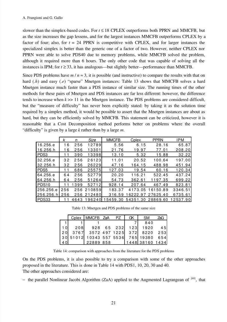
slower than the simplex-based codes. For t ≤ 18 CPLEX outperforms both PPRN and MMCFB, butas the size increases the gap lessens, and for the largest instances MMCFB outperforms CPLEX by afactor of four; also, for t = 24 PPRN is competitive with CPLEX, and for larger instances thespecialized simplex is better than the generic one of a factor of two. However, neither CPLEX nor
PPRN were able to solve PDS40 due to memory problems, while MMCFB solved the problem,although it required more than 6 hours. The only other code that was capable of solving all theinstances is IPM; for t ≥ 33, it has analogous—but slightly better—performance than MMCFB.
Since PDS problems have m / n ≈ 3, it is possible (and instructive) to compare the results with that onhard (.h) and easy (.e) “sparse” Mnetgen instances: Table 13 shows that MMCFB solves a hardMnetgen instance much faster than a PDS instance of similar size. The running times of the othermethods for these pairs of Mnetgen and PDS instances are far less different: however, the differencetends to increase when k >> 11 in the Mnetgen instance. The PDS problems are considered difficult,but the “measure of difficulty” has never been explicitly stated: by taking it as the solution time
required by a simplex method, it would be possible to assert that the Mnetgen instances are about ashard, but they can be efficiently solved by MMCFB. This statement can be criticized, however it isreasonable that a Cost Decomposition method performs better on problems where the overall“difficulty” is given by a large k rather than by a large m.
k n Size MMCFB Cplex PPRN IPM
16.256.e 1 6 2 5 6 1 2 7 8 9 5 .56 6 .15 28.16 65.87
16.256.h 1 6 2 5 6 1 3 3 0 1 21.76 19 .97 77.01 208.20
PDS3 1 1 3 9 0 1 3 3 9 8 13.10 5 .32 15.88 32.22
32.256.e 3 2 2 5 6 2 61 2 3 11.01 20 .52 100.64 197.00
32.256.h 3 2 2 56 2 6 2 2 9 47.16 164 .15 488.98 451.94
PDS5 1 1 6 8 6 2 5 5 7 5 127.03 19 .54 60.16 120.3464.256.e 6 4 2 56 5 2 7 7 9 20.20 116 .21 522.45 437.24
64.256.h 6 4 2 56 5 1 2 6 4 54.73 362 .61 1197.35 699.22
PDS10 1 1 1 3 9 9 5 2 7 1 2 928.14 207 .64 467.49 823.81
256.256.e 2 5 6 2 5 6 2 1 08 5 9 1 83 .3 7 4 17 3. 05 1 61 50 .8 9 3 34 6. 51
25 6.256. h 2 5 6 2 5 6 2 1 24 8 0 3 16 .5 9 1 62 22 .9 7 2 76 25 .4 0 6 73 5. 61
PDS33 1 1 4 6 4 3 1 9 6 2 4 0 1 54 59 . 30 5 43 5 1. 30 2 88 6 9. 60 1 2 53 7. 9 0
Table 13: Mnetgen and PDS problems of the same size
Cplex MMCFB ZaA PZ GK SM ZaG
1 1 1 7 8 4 0
1 0 2 0 8 9 2 8 6 5 2 3 2 1 2 3 1 9 2 0 4 5
2 0 3 7 6 7 3 5 7 2 4 97 1 2 2 5 3 72 8 2 2 0 2 53
3 0 51 01 2 1 03 43 5 57 55 3 6 7 6 5 19 38 0 6 5 4
4 0 2 2 8 8 9 8 5 8 1 4 4 8 3 8 1 6 0 1 4 3 4
Table 14: comparison with approaches from the literature for the PDS problems
On the PDS problems, it is also possible to try a comparison with some of the other approachesproposed in the literature. This is done in Table 14 with PDS1, 10, 20, 30 and 40.The other approaches considered are:
− the parallel Nonlinear Jacobi Algorithm (ZaA) applied to the Augmented Lagrangean of [69], that

8/7/2019 A bundle type dual-ascent approach to linear multicommodity min-cost flow problems
http://slidepdf.com/reader/full/a-bundle-type-dual-ascent-approach-to-linear-multicommodity-min-cost-flow-problems 22/30
A Bundle-type approach to Multicommodity flow problems
22
was run on a Thinking Machine CM-5 with 64 processors, each one (apparently) capable of about25 SPECfp92;
− the linear-quadratic exact penalty function method (PZ) of [61], that was run on a Cray Y-MP vectorsupercomputer, whose performances with respect to scalar architectures are very hard to assess;
− the ε-approximation algorithm (GK) of [33], that was run on a IBM RS6000-550 workstation (83.3SPECfp92, 40.7 SPECint92); the largest instances were solved to the precision of 4-5 significantdigits;
− the specialized Interior Point method (SM) of [62], that was run on a DECstation 3100 (whoseSPEC figures are unknown to us) and that obtained solutions with 8 digits accuracy;
− a modification and parallelization of the above (ZaG) that was run on a cluster of SPARCstation 20workstations [70]; unfortunately, the exact model is not specified, so that the (SPECfp92,SPECint92) can be anything between (80.1, 76.9) and (208.2, 169.4).
Unfortunately, extracting significant information from the figures is very difficult due to the differentmachine used. However, it is clear that, for these instances, the ε-approximation algorithm providesgood solutions in a very low time: in Table 15, optimal objective function values (obtained withCPLEX), lower bounds obtained by MMCFB and upper bounds obtained by GK are compared. Thereported Gaps for GK are directly drawn from [33], except for the last two problems for which anestimate of the exact optimal objective function value had been used in [33].
Cplex MMCFB GK
n O.F. Value O.F. Value Gap O.F. Value Gap
1 2 9 0 8 3 9 3 0 5 2 3 2 9 0 8 3 9 0 6 6 5 8 -8 e -0 7 2 . 9 0 8 3 9 E +1 0 3 e -0 9
2 2 8 8 5 7 8 6 2 0 1 0 2 8 8 5 7 8 3 8 0 0 2 -8 e -0 7 2 . 8 8 5 7 9 E +1 0 6 e -0 83 2 8 5 9 7 3 7 4 1 4 5 2 8 5 9 7 3 4 8 6 1 4 -9 e -0 7 2 . 8 5 9 7 4 E +1 0 1 e -0 8
4 2 8 3 4 1 9 2 8 5 8 1 2 8 3 4 1 9 0 3 3 9 6 -9 e -0 7 2 . 8 3 4 1 9 E +1 0 2 e -0 7
5 2 8 0 5 4 0 5 2 6 0 7 2 8 0 5 4 0 3 5 8 0 3 -6 e -0 7 2 . 8 0 5 4 1 E +1 0 3 e -0 7
6 2 7 7 6 1 0 3 7 6 0 0 2 7 7 6 1 0 1 5 9 1 5 -8 e -0 7 2 . 7 7 6 1 1 E +1 0 5 e -0 7
7 2 7 5 1 0 3 7 7 0 1 3 2 7 5 1 0 2 5 3 7 6 2 -4 e -0 6 2 . 7 5 1 0 7 E +1 0 1 e -0 5
8 2 7 2 3 9 6 2 7 2 1 0 2 7 2 3 9 6 0 3 6 3 4 -9 e -0 7 2 . 7 2 3 9 9 E +1 0 9 e -0 6
9 2 6 9 7 4 5 8 6 2 4 1 2 6 9 7 4 4 5 6 1 6 7 -5 e -0 6 2 . 6 9 7 4 9 E +1 0 1 e -0 5
1 0 2 6 7 2 7 09 4 9 7 6 2 6 7 2 7 03 8 8 3 0 -2 e - 0 6 2 .6 7 28 0E +1 0 3 e -0 5
2 0 2 3 8 2 1 65 8 6 4 0 2 3 8 2 1 63 7 8 4 1 -9 e - 0 7 2 .3 8 23 2E +1 0 7 e -0 5
3 0 2 1 3 8 5 44 5 7 3 6 2 1 3 8 5 44 3 2 6 2 -1 e - 0 7 2 .1 3 88 8E +1 0 2 e -0 4
4 0 1 8 8 5 5 19 8 8 2 4 1 8 8 5 5 18 1 4 5 6 -9 e - 0 7 1 .8 8 59 5E +1 0 2 e -0 4
Table 15: comparison of the relative gap of MMCFB and GK
Among the other methods, the two parallel ones seem to provide good results, since MMCFB couldnot surely achieve a speedup larger than 11 (on the same machines): however, the comparison is verydifficult, and it is perhaps better not to attempt any comment. A remark can instead be done about theconcept of “solution” that is underneath some of the figures in the table: many of the codes—forinstance (GK), (SM) and (ZaG)—use heuristic stopping criteria, essentially performing a fixednumber of iterations before stopping. A posteriori, the solutions are found to be accurate, but thealgorithm is not capable of “certifying” it by means of appropriate primal-dual estimates of the gap.

8/7/2019 A bundle type dual-ascent approach to linear multicommodity min-cost flow problems
http://slidepdf.com/reader/full/a-bundle-type-dual-ascent-approach-to-linear-multicommodity-min-cost-flow-problems 23/30
A. Frangioni and G. Gallo
23
5.4 The JLF problems
k n m b Size MMCFB Cplex PPRN I PM LOQO IPCplex
1 0 t e r m 1 0 1 9 0 5 1 0 1 4 6 5 1 0 0 0 . 2 7 0 . 8 4 1 . 0 7 9 . 1 6 2 6 . 1 7 1 0 . 9 7
10term.0 1 0 1 9 0 5 0 7 1 4 3 5 0 7 0 0 . 2 3 0 . 7 8 0 . 7 0 7 . 0 4 2 8 . 2 9 1 3 . 1 0
10t erm.50 1 0 1 9 0 4 9 8 1 3 4 4 9 8 0 2 . 0 0 0 . 8 2 1 . 2 2 7 . 9 7 1 8 . 0 5 1 1 . 6 010t er m. 100 1 0 1 9 0 4 9 1 1 2 7 4 91 0 2 . 4 0 0 . 8 6 1 . 1 0 8 . 6 9 1 9 . 2 1 1 0 . 5 8
1 5 t e r m 1 5 2 8 5 7 9 6 2 5 3 1 19 40 4 . 8 1 3 . 3 9 1 1 . 5 7 4 1 . 3 5 2 1 0 . 9 4 1 0 6 . 9 8
15term.0 1 5 2 8 5 7 4 5 2 0 2 1 11 75 1 . 9 4 2 . 7 2 1 0 . 2 3 3 0 . 3 5 1 2 3 . 2 1 4 7 . 1 5
Chen0 4 2 6 1 1 7 4 3 4 6 8 0 . 3 0 0 . 2 5 0 . 3 2 0 . 2 5 0 . 4 4 0 . 3 8
Chen1 5 3 6 1 7 4 6 5 8 7 0 0 . 9 8 0 . 6 4 0 . 7 3 0 . 4 1 0 . 9 9 0 . 7 7
Chen2 7 4 1 3 5 8 1 5 5 2 5 0 6 5 . 9 8 4 . 8 9 3 . 7 7 1 . 5 9 4 . 1 7 3 . 9 1
Chen3 1 5 3 1 1 4 9 5 6 2 2 3 5 1 . 2 2 5 . 1 8 1 . 9 6 1 . 1 0 3 . 1 2 2 . 6 2
Chen4 1 5 5 5 4 2 0 1 7 6 6 3 0 0 2 5 . 4 9 8 3 . 3 9 2 0 . 0 5 5. 9 2 4 6 . 9 2 3 2 . 7 5Chen5 1 0 6 5 5 6 9 2 4 2 5 6 9 0 5 2 . 5 8 4 8 . 7 4 4 8 . 1 2 5. 2 4 2 1 . 1 8 1 5 . 5 3
assad1.5k 3 4 7 9 8 9 8 2 9 4 0 . 0 3 0 . 1 1 0 . 0 9 0 . 3 6 0 . 3 9 0 . 2 2
assad1.6k 3 4 7 9 8 9 8 2 9 4 0 . 0 1 0 . 0 8 0 . 0 6 0 . 3 9 0 . 3 7 0 . 2 2assad3.4k 6 8 5 2 0 4 9 5 1 2 2 4 0 . 0 8 0 . 3 3 0 . 5 5 1 . 4 1 4 . 2 6 1 . 4 4
assad3.7k 6 8 5 2 0 4 9 5 1 2 2 4 0 . 1 0 0 . 2 9 0 . 5 6 1 . 5 7 4 . 2 2 1 . 4 1
Table 16: results for some of the JLF problems
Table 16 shows the results obtained on some JLF problems, those with SPT subproblems: despite thesmall number of commodities, MMCFB is still competitive on the “xterm.y” and “Assadx.y” sets.The “Chenx” problems are more “difficult” than the others, since they require an order of magnitudemore time to be solved than the “xterm.y” instances of comparable size. For this data set, the InteriorPoint codes are competitive with, and IPM largely outperforms, all the others, confirming the
potential advantage of the Interior Point technology on “hard” instances. However, such smallMMCF s are well in the range of general-purpose LP solvers, so that it makes little sense to use ad-hoc technology. In this case, other issues such as availability, ease-of-use and reoptimization shouldbe taken into account.
5.5 The dimacs2pprn problems
Due to the previous results, the general-purpose Interior Point codes were not run on this data set,that contains the largest instances of all. As described in §4.5, for any given dimension a hard and aneasy instance have been constructed: the results are separately reported in Table 17 and Table 18
respectively (note the difference in the number of mutual capacity constraints, b). As in the Mnetgencase, CPLEX ran out of memory on the largest instances, and PPRN was sometimes stopped afterhaving run for a very long time without producing a result (the “+” entries): IPM also experiencedmemory problems on the largest instances, with 1.2 millions of variables. Note that a 2.5.105
variables MMCF requires about 11, 20 and 129 megabytes of memory to be solved by MMCFB,PPRN and CPLEX respectively: MMCFB requires an order of magnitude less memory than CPLEX.
The results obtained from these instances confirm those obtained from the previous data sets:MMCFB is faster than the two simplex-based codes on all but the smallest instances, IPM iscompetitive with both CPLEX and PPRN on instances with large k but MMCFB is even more
efficient—for k = 256 it is always more than an order of magnitude faster than the other codes,

8/7/2019 A bundle type dual-ascent approach to linear multicommodity min-cost flow problems
http://slidepdf.com/reader/full/a-bundle-type-dual-ascent-approach-to-linear-multicommodity-min-cost-flow-problems 24/30
A Bundle-type approach to Multicommodity flow problems
24
approaching the three orders of magnitude as m increases. Yet, especially on large problems,MMCFB spends most of the time in the SPT solver, which suggests that substantial improvementsshould be obtained by making use of reoptimization techniques in the SPT algorithms.
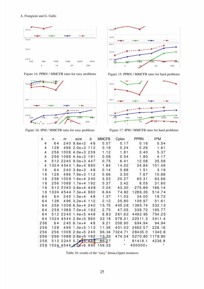
The results are also illustrated by Figure 12, Figure 13, Figure 14, Figure 15, Figure 16 and Figure
17, where the ratio of the running times of CPLEX, PPRN and IPM vs. MMCFB is reported for“hard” and “easy” instances separately. It is interesting to note that the relative efficiency of MMCFBwith respect to the simplex-based codes for k = 4 is lower on easy problems than on hard ones, whilethe converse is true for the relative efficiency of MMCFB with respect to IPM.
k n m size b MMCFB Cplex PPRN IPM
4 6 4 2 4 0 9.6e+2 2 4 0 0 .46 0 .32 0 .37 1 .23
4 1 2 8 4 9 6 2.0e+3 1 1 2 1 .30 1 .05 2 .36 2 .65
4 2 5 6 1 0 0 8 4.0e+3 1 0 0 7 21 .50 8 .85 14.82 23.13
4 2 5 6 1 0 8 8 4.4e+3 1 9 2 0 .36 1 .38 2 .22 8 .86
4 5 1 2 2 2 4 0 9.0e+3 4 4 7 5 .97 14 .39 32.26 63.44
4 1 02 4 4 54 4 1.8e+4 9 6 0 39 .76 70 .41 178.06 266.791 6 6 4 2 4 0 3.8e+3 2 4 0 0 .44 1 .23 1 .68 7 .58
1 6 1 2 8 4 9 6 7.9e+3 1 1 2 4 .31 19 .72 29.75 24.74
1 6 2 5 6 1 00 8 1.6e+4 2 4 0 64 .79 23 0.82 5 50.1 1 4 37.4 1
1 6 2 5 6 1 0 8 8 1.7e+4 1 9 2 1 .08 5 .38 22.14 39.70
1 6 5 1 2 2 24 0 3.6e+4 4 4 8 14 .15 21 8.55 4 79.9 6 5 40.9 0
1 6 1 0 2 4 4 5 4 4 7. 3e +4 9 6 0 6 9 .5 9 1 07 9 .6 3 2 7 96 .8 5 2 3 63 .0 2
6 4 6 4 2 4 0 1.5e+4 2 4 0 2 .89 50 .70 92.77 51.55
6 4 1 28 4 96 3.2e+4 1 12 9 .23 222.65 562.71 410.42
6 4 2 5 6 1 0 0 8 6 .5 e+ 4 1 0 0 8 9 4 .0 7 3 25 6 .5 2 1 00 11 .3 0 4 55 6. 5 7
6 4 2 56 1 08 8 7.0e+4 1 92 4 .37 93 .14 535.47 283.19
6 4 5 1 2 2 2 4 0 1. 4e+ 5 4 4 8 3 7. 69 2 36 2. 37 7 14 6. 33 2 70 3. 51
6 4 1 0 2 4 4 5 4 4 2 .9 e+ 5 9 6 0 2 1 5 .7 0 1 87 6 3. 9 5 2 78 7. 6 2 28 99 . 4
2 5 6 6 4 2 4 0 6.1e+4 2 4 0 17 .52 668.27 1415.55 258.87
2 5 6 1 2 8 4 9 6 1.3e+5 1 1 2 4 8. 72 3 52 5. 27 1 14 43 .5 0 5 01 .8 0
2 5 6 2 5 6 1 0 0 8 2 .6 e+ 5 1 0 0 8 45 8 .3 6 56 7 56 .9 2 0 0 0 0 0 + 6 06 9. 4 6
2 5 6 2 5 6 1 0 88 2.8e+5 1 9 2 1 5. 30 8 21 .8 6 7 83 2. 38 1 47 5. 91
2 5 6 5 1 2 2 24 0 5.7e+5 4 4 8 218 .84 * 13 8225. 0 2 2266. 8
2 5 6 1 0 2 4 4 5 4 4 1.2e+6 9 6 0 898 .51 * 4 0 0 0 0 0 + *
Table 17: results of the “hard” dimacs2pprn instances
1 e + 0
1 e + 1
1 e + 2
2 4 0 4 9 6 1 0 0 8 1 0 8 8 2 2 4 0 4 5 4 4
4 1 6 6 4 2 5 6
Figure 12: CPLEX / MMCFB ratio for easy problems
1 e - 1
1 e + 0
1 e + 1
1 e + 2
1 e + 3
2 4 0 4 9 6 1 0 0 8 1 0 8 8 2 2 4 0 4 5 4 4
4 1 6 6 4 2 5 6
Figure 13: CPLEX / MMCFB ratio for hard problems
8/7/2019 A bundle type dual-ascent approach to linear multicommodity min-cost flow problems
http://slidepdf.com/reader/full/a-bundle-type-dual-ascent-approach-to-linear-multicommodity-min-cost-flow-problems 25/30
A. Frangioni and G. Gallo
25
1e+0
1e+1
1e+2
1e+3
2 4 0 4 9 6 1 0 0 8 1 0 8 8 2 2 4 0 4 5 4 4
4 1 6 6 4 2 5 6
Figure 14: PPRN / MMCFB ratio for easy problems
1 e - 1
1e+0
1e+1
1e+2
1e+3
2 4 0 4 9 6 1 0 0 8 1 0 8 8 2 2 4 0 4 5 4 4
4 1 6 6 4 2 5 6
Figure 15: PPRN / MMCFB ratio for hard problems
1e+0
1e+1
1e+2
2 4 0 4 9 6 1 0 0 8 1 0 8 8 2 2 4 0 4 5 4 4
4 1 6 6 4 2 5 6
Figure 16: IPM / MMCFB ratio for easy problems
1e+0
1e+1
1e+2
2 4 0 4 9 6 1 0 0 8 1 0 8 8 2 2 4 0 4 5 4 4
4 1 6 6 4 2 5 6
Figure 17: IPM / MMCFB ratio for hard problems
k n m size b MMCFB Cplex PPRN IPM
4 6 4 2 4 0 9.6e+2 4 8 0 .07 0 .17 0 .16 0 .54
4 1 2 8 4 9 6 2.0e+3 1 1 2 0 .18 0 .24 0 .26 1 .61
4 2 5 6 1 0 0 8 4.0e+3 2 3 9 1 .12 1 .81 3 .40 5 .374 2 5 6 1 0 8 8 4.4e+3 1 9 1 0 .08 0 .54 1 .80 4 .17
4 5 1 2 2 2 4 0 9.0e+3 4 4 7 0 .75 6 .41 12.08 35.58
4 1 02 4 4 54 4 1.8e+4 9 60 1 .84 14.02 34.84 101.49
1 6 6 4 2 4 0 3.8e+3 4 8 0 .14 0 .88 1 .51 3 .19
1 6 1 2 8 4 9 6 7.9e+3 1 1 2 0 .66 3 .50 7 .67 10.88
1 6 2 56 1 0 0 8 1.6e+4 2 40 3 .53 20.27 65.31 63.66
1 6 2 5 6 1 0 8 8 1.7e+4 1 9 2 0 .37 3 .42 8 .05 31.60
1 6 5 1 2 2 24 0 3.6e+4 4 4 8 2 .24 43.30 275.89 166.14
1 6 1 0 24 4 5 4 4 7.3e+4 9 6 0 6 .6 4 7 4. 82 1 28 6. 26 5 14 .7 4
6 4 6 4 2 4 0 1.5e+4 4 8 1 .37 11.03 34.00 19.72
6 4 1 28 4 96 3.2e+4 1 12 2 .12 25.80 109.97 51.616 4 2 5 6 1 0 0 8 6.5e+4 2 4 0 1 5. 75 4 45 .2 8 1 39 5. 74 3 33 .1 3
6 4 2 5 6 1 08 8 7.0e+4 1 9 2 2 .75 47.05 339.72 195.77
6 4 5 1 2 2 2 4 0 1.4e+5 4 4 8 8 .8 3 2 61 .6 2 4 49 2. 95 7 54 .2 5
6 4 1 0 2 4 4 5 4 4 2 .9e +5 9 6 0 3 2. 18 9 78 .3 1 2 25 11 .3 3 41 1. 4
2 56 6 4 2 40 6.1e+4 4 8 9 .21 208.90 694.94 94.94
2 5 6 1 2 8 4 9 6 1.3e+5 1 1 2 1 1.36 4 01.0 2 2 662.5 7 228. 16
2 5 6 2 5 6 1 0 0 8 2 .6e +5 2 4 0 9 6. 34 7 32 4. 71 2 84 35 .0 1 34 0. 8
2 5 6 2 5 6 1 0 8 8 2 .8e +5 1 9 2 1 3. 33 4 74 .3 4 5 27 0. 80 1 17 8. 85
2 5 6 5 1 2 2 24 0 5.7e+5 4 4 8 85.17 * 81419.1 4236.8
2 5 6 1 0 2 4 4 5 4 4 1.2e+6 9 60 159.33 * 4 0 0 0 0 0 + *
Table 18: results of the “easy” dimacs2pprn instances

8/7/2019 A bundle type dual-ascent approach to linear multicommodity min-cost flow problems
http://slidepdf.com/reader/full/a-bundle-type-dual-ascent-approach-to-linear-multicommodity-min-cost-flow-problems 26/30
A Bundle-type approach to Multicommodity flow problems
26
5.6 The BHV problems
MMCFB Cplex BCG
I t e r Time Time I te r Time
q1 4 2 0 .63 7 .93 4 5 .06
q2 3 4 0 .51 9 .03 5 4 .15q3 4 2 0 .63 12.45 5 5 .15
q4 5 5 0 .83 16.08 6 6 .78
q5 8 5 1 .33 20.3 6 6 .78
q6 1 0 0 1 .55 26.75 7 7 .78
q7 1 0 0 1 .58 31.07 7 8 .69
q8 1 56 2 .66 37.41 8 10.66
q9 2 21 3 .76 44.96 8 10.60
q10 1 7 2 2 .92 51.95 9 12.88
q11 1 9 6 3 .37 61.58 8 12.55
q12 2 7 0 4 .75 64.96 9 15.95
Table 19: results for the “px” problems
MMCFB Cplex BCG
I t e r Time Time I t e r Time
r 1 0 - 5 - 1 2 5 8 .73 6570.19 4 3 91 6 6 2
r 1 0 - 5 - 2 2 6 9 .01 9249.35 4 2 08 6 0 7r 1 0 - 5 - 3 3 8 13. 02 659 8.73 3 23 7 3 9 8
r 1 0 - 5 - 4 2 0 7 .14 8481.97 4 1 49 5 0 1
r 1 0 - 5 - 5 2 3 8 .16 9262.55 3 6 33 4 2 0
r 1 0 - 5 5 - 1 8 7 7 311 .01 108 43.10 2 45 5 1 6 2
r 1 0 - 5 5 - 2 9 3 4 330 .21 129 78.80 2 69 0 1 9 9
r 1 0 - 5 5 - 3 1 2 43 44 5. 27 13 84 9. 00 2 6 9 4 2 2 4
r 1 0 - 5 5 - 4 9 9 9 349 .20 115 81.60 2 51 1 2 1 8
r 1 0 - 5 5 - 5 87 7 318 .00 * 2 7 0 6 2 3 4
Table 20: results for the “r10-x-y” problems
Among the available specialized solvers, only MMCFB is capable of solving undirected instances; thethree general-purpose LP solvers can be adapted for the task, but, due to the very poor resultsobtained by the IP codes, only CPLEX was actually run on these data sets. The times for the ColumnGeneration algorithm (BCG) were obtained on an IBM RS6000-590 workstation, credited for 121.6SPECint92 and 259.7 SPECfp92, i.e. essentially twice as fast as the HP9000/712-80: Table 19shows that on the easy “px” problems MMCFB is 10 times faster than BCG. The results on the otherdata set, shown in Table 20, are quite surprising: the two methods are essentially equivalent on the(highly fractional) “r10-55-y” instances, but MMCFB is able to solve the similar (integral) “r10-5-y”instances 30 times faster, while BCG needs about twice the time. A rationale for the behavior of MMCFB exists: a smaller number of trees is likely to be necessary to form the optimal flow as aconvex combination in the integral data case. However, it is unclear why the same should not be truefor the CG code: should it be proved that this is due to the Bundle-type approach, the result could berather interesting.
5.7 Conclusions
The above computational experience shows that MMCFB can be a valuable tool for solving MMCF s
with many commodities: to stress one figure, MMCFB solved the hard, dense (256, 256) Mnetgeninstances in less than 20 minutes, but more than 6 and 10 days were needed by CPLEX and PPRNrespectively, while IPM required a little less than 5 hours. As the experience with the dimacs2pprndata set shows, MMCF s with over one million of variables can be solved in less than 15 minutes of CPU time by a low-end computer, provided that the subproblems have a SPT structure. In acompanion paper[14], we also show that a somewhat “naïve” parallelization of MMCFB obtains verygood parallel efficiencies on a massively-parallel computer for the same instances for which thesequential code is more competitive, i.e. when k is large. Conversely, MMCFB does not appear to bea good choice for problems with a small number of commodities, unless the instances are very large:the PDS problems show that MMCFB can be competitive even on problems with m / k ratio largerthan 1000, but the speedup with respect to simplex-based codes is far smaller than on many-
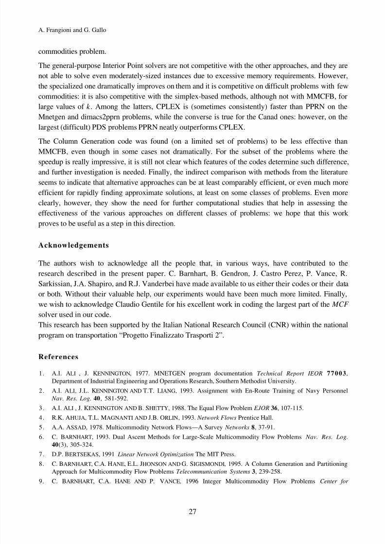
8/7/2019 A bundle type dual-ascent approach to linear multicommodity min-cost flow problems
http://slidepdf.com/reader/full/a-bundle-type-dual-ascent-approach-to-linear-multicommodity-min-cost-flow-problems 27/30
A. Frangioni and G. Gallo
27
commodities problem.
The general-purpose Interior Point solvers are not competitive with the other approaches, and they arenot able to solve even moderately-sized instances due to excessive memory requirements. However,the specialized one dramatically improves on them and it is competitive on difficult problems with few
commodities: it is also competitive with the simplex-based methods, although not with MMCFB, forlarge values of k . Among the latters, CPLEX is (sometimes consistently) faster than PPRN on theMnetgen and dimacs2pprn problems, while the converse is true for the Canad ones: however, on thelargest (difficult) PDS problems PPRN neatly outperforms CPLEX.
The Column Generation code was found (on a limited set of problems) to be less effective thanMMCFB, even though in some cases not dramatically. For the subset of the problems where thespeedup is really impressive, it is still not clear which features of the codes determine such difference,and further investigation is needed. Finally, the indirect comparison with methods from the literatureseems to indicate that alternative approaches can be at least comparably efficient, or even much more
efficient for rapidly finding approximate solutions, at least on some classes of problems. Even moreclearly, however, they show the need for further computational studies that help in assessing theeffectiveness of the various approaches on different classes of problems: we hope that this workproves to be useful as a step in this direction.
Acknowledgements
The authors wish to acknowledge all the people that, in various ways, have contributed to theresearch described in the present paper. C. Barnhart, B. Gendron, J. Castro Perez, P. Vance, R.
Sarkissian, J.A. Shapiro, and R.J. Vanderbei have made available to us either their codes or their dataor both. Without their valuable help, our experiments would have been much more limited. Finally,we wish to acknowledge Claudio Gentile for his excellent work in coding the largest part of the MCF
solver used in our code.This research has been supported by the Italian National Research Council (CNR) within the nationalprogram on transportation “Progetto Finalizzato Trasporti 2”.
References
1. A.I. ALI , J. KENNINGTON, 1977. MNETGEN program documentation Technical Report IEOR 77003,
Department of Industrial Engineering and Operations Research, Southern Methodist University.2. A.I. ALI, J.L. KENNINGTON AND T.T. LIANG, 1993. Assignment with En-Route Training of Navy Personnel
Nav. Res. Log. 40, 581-592.
3. A.I. ALI , J. KENNINGTON AND B. SHETTY, 1988. The Equal Flow Problem EJOR 36, 107-115.
4. R.K. AHUJA, T.L. MAGNANTI AND J.B. ORLIN, 1993. Network Flows Prentice Hall.
5. A.A. ASSAD, 1978. Multicommodity Network Flows—A Survey Networks 8, 37-91.
6. C. BARNHART, 1993. Dual Ascent Methods for Large-Scale Multicommodity Flow Problems Nav. Res. Log.
40(3), 305-324.
7. D.P. BERTSEKAS, 1991 Linear Network Optimization The MIT Press.
8. C. BARNHART, C.A. HANE, E.L. JHONSON AND G. SIGISMONDI, 1995. A Column Generation and PartitioningApproach for Multicommodity Flow Problems Telecommunication Systems 3, 239-258.
9. C. BARNHART, C.A. HANE AND P. VANCE, 1996 Integer Multicommodity Flow Problems Center for
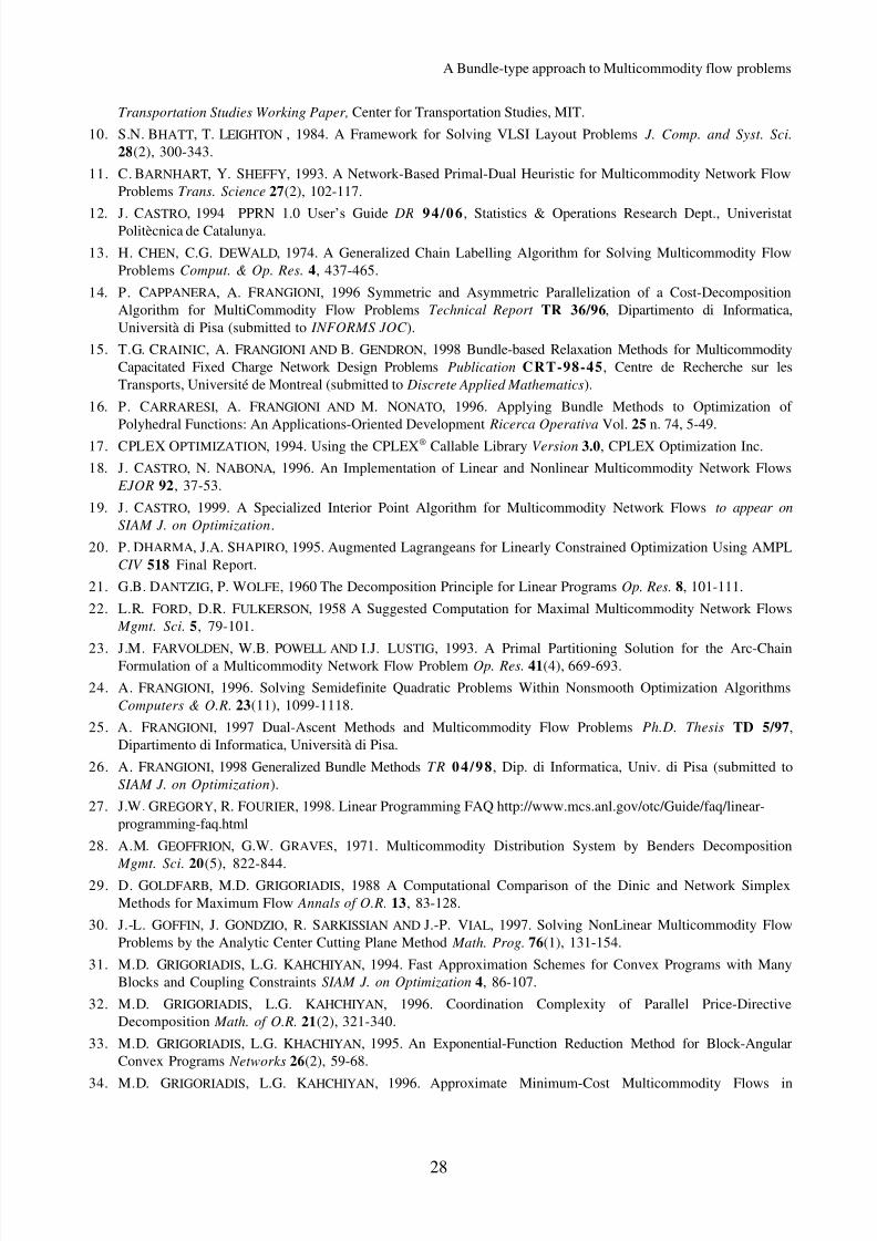
8/7/2019 A bundle type dual-ascent approach to linear multicommodity min-cost flow problems
http://slidepdf.com/reader/full/a-bundle-type-dual-ascent-approach-to-linear-multicommodity-min-cost-flow-problems 28/30
A Bundle-type approach to Multicommodity flow problems
28
Transportation Studies Working Paper, Center for Transportation Studies, MIT.
10. S.N. BHATT, T. LEIGHTON , 1984. A Framework for Solving VLSI Layout Problems J. Comp. and Syst. Sci.
28(2), 300-343.
11. C. BARNHART, Y. SHEFFY, 1993. A Network-Based Primal-Dual Heuristic for Multicommodity Network FlowProblems Trans. Science 27(2), 102-117.
12. J. CASTRO, 1994 PPRN 1.0 User’s Guide DR 94/06 , Statistics & Operations Research Dept., UniveristatPolitècnica de Catalunya.
13. H. CHEN, C.G. DEWALD, 1974. A Generalized Chain Labelling Algorithm for Solving Multicommodity FlowProblems Comput. & Op. Res. 4, 437-465.
14. P. CAPPANERA, A. FRANGIONI, 1996 Symmetric and Asymmetric Parallelization of a Cost-DecompositionAlgorithm for MultiCommodity Flow Problems Technical Report TR 36/96, Dipartimento di Informatica,Università di Pisa (submitted to INFORMS JOC ).
15. T.G. CRAINIC, A. FRANGIONI AND B. GENDRON, 1998 Bundle-based Relaxation Methods for MulticommodityCapacitated Fixed Charge Network Design Problems Publication CRT-98-45, Centre de Recherche sur lesTransports, Université de Montreal (submitted to Discrete Applied Mathematics).
16. P. CARRARESI, A. FRANGIONI AND M. NONATO, 1996. Applying Bundle Methods to Optimization of Polyhedral Functions: An Applications-Oriented Development Ricerca Operativa Vol. 25 n. 74, 5-49.
17. CPLEX OPTIMIZATION, 1994. Using the CPLEX® Callable Library Version 3.0, CPLEX Optimization Inc.
18. J. CASTRO, N. NABONA, 1996. An Implementation of Linear and Nonlinear Multicommodity Network FlowsEJOR 92, 37-53.
19. J. CASTRO, 1999. A Specialized Interior Point Algorithm for Multicommodity Network Flows to appear on
SIAM J. on Optimization.
20. P. DHARMA, J.A. SHAPIRO, 1995. Augmented Lagrangeans for Linearly Constrained Optimization Using AMPLCIV 518 Final Report.
21. G.B. DANTZIG, P. WOLFE, 1960 The Decomposition Principle for Linear Programs Op. Res. 8, 101-111.
22. L.R. FORD, D.R. FULKERSON, 1958 A Suggested Computation for Maximal Multicommodity Network FlowsMgmt. Sci. 5, 79-101.
23. J.M. FARVOLDEN, W.B. POWELL AND I.J. LUSTIG, 1993. A Primal Partitioning Solution for the Arc-ChainFormulation of a Multicommodity Network Flow Problem Op. Res. 41(4), 669-693.
24. A. FRANGIONI, 1996. Solving Semidefinite Quadratic Problems Within Nonsmooth Optimization AlgorithmsComputers & O.R. 23(11), 1099-1118.
25. A. FRANGIONI, 1997 Dual-Ascent Methods and Multicommodity Flow Problems Ph.D. Thesis TD 5/97,Dipartimento di Informatica, Università di Pisa.
26. A. FRANGIONI, 1998 Generalized Bundle Methods TR 04/98, Dip. di Informatica, Univ. di Pisa (submitted toSIAM J. on Optimization).
27. J.W. GREGORY, R. FOURIER, 1998. Linear Programming FAQ http://www.mcs.anl.gov/otc/Guide/faq/linear-programming-faq.html
28. A.M. GEOFFRION, G.W. GRAVES, 1971. Multicommodity Distribution System by Benders Decomposition
Mgmt. Sci. 20(5), 822-844.29. D. GOLDFARB, M.D. GRIGORIADIS, 1988 A Computational Comparison of the Dinic and Network SimplexMethods for Maximum Flow Annals of O.R. 13, 83-128.
30. J.-L. GOFFIN, J. GONDZIO, R. SARKISSIAN AND J.-P. VIAL, 1997. Solving NonLinear Multicommodity FlowProblems by the Analytic Center Cutting Plane Method Math. Prog. 76(1), 131-154.
31. M.D. GRIGORIADIS, L.G. KAHCHIYAN, 1994. Fast Approximation Schemes for Convex Programs with ManyBlocks and Coupling Constraints SIAM J. on Optimization 4, 86-107.
32. M.D. GRIGORIADIS, L.G. KAHCHIYAN, 1996. Coordination Complexity of Parallel Price-DirectiveDecomposition Math. of O.R. 21(2), 321-340.
33. M.D. GRIGORIADIS, L.G. KHACHIYAN, 1995. An Exponential-Function Reduction Method for Block-AngularConvex Programs Networks 26(2), 59-68.
34. M.D. GRIGORIADIS, L.G. KAHCHIYAN, 1996. Approximate Minimum-Cost Multicommodity Flows in
8/7/2019 A bundle type dual-ascent approach to linear multicommodity min-cost flow problems
http://slidepdf.com/reader/full/a-bundle-type-dual-ascent-approach-to-linear-multicommodity-min-cost-flow-problems 29/30
A. Frangioni and G. Gallo
29
O(ε-2KNM ) time Math. Prog. 75(3), 477-482.35. G. GALLO, S. PALLOTTINO, 1988. Shortest Path Algorithms Annals of O.R. 13, 3-79.
36. N. GARG, V.V. VAZIRANI AND M. YANNAKAKIS, 1993. Approximate Max-Flow Min-(Multi)Cut Theorems andtheir Applications Proc. 25th STOC , 698-707.
37. J.K. HO, E. LOUTE, 1981. An advanced implementation of the Dantzig Wolfe decomposition algorithm for linear
programming Math. Prog. 20(1), 303-326.38. J.K. HO, E. LOUTE, 1983. Computational Experience with Advanced Implementation of Decomposition
Algorithms for Linear Programming Math. Prog. 27(3), 283-290.
39. J-B. HIRIART-URRUTY, C. LEMARÉCHAL, 1993. Convex Analysis and Minimization Algorithms A Series of Comprehensive Studies in Mathematics, vol. 306, Springer-Verlag.
40. M. HELD, P. WOLFE AND H. CROWDER, 1974. Validation of Subgradient Optimization Math. Prog. 6, 62-88.
41. K.L. JONES , I.J. LUSTIG, 1992. Input Format for Multicommodity Flow Problems Program in Statistics and
Operations Research, Department of Civil Engineering and Operations Research, Princeton University .
42. K.L. JONES , I.J. LUSTIG, J.M. FARVOLDEN AND W.B. POWELL, 1993. Multicommodity Network Flows: TheImpact of Formulation on Decomposition Math. Prog. 62, 95-117.
43. P. KLEIN, A. AGRAWAL, R. RAVI AND S. RAO, 1990. Approximation Through Multicommodity Flow Proc.
31th FOCS, 726-727.44. J.E. KELLEY, 1960. The Cutting-Plane Method for Solving Convex Programs Journal of the SIAM 8, 703-712.
45. J.L. KENNINGTON, 1978. A Survey of Linear Cost Multicommodity Network Flows Op. Res. 26(2), 209-236.
46. J.L. KENNINGTON, 1978. A Primal Partitioning Code for Solving Multicommodity Flow Problems Technical
Report 79008, Department of Industrial Engineering and Operations Research, Southern Methodist University.
47. K.C. KIWIEL, 1990. Proximity Control in Bundle Methods for Convex Nondifferentiable Optimization Math.
Prog. 46, 05-122.
48. A.P. KAMATH, N.K. KARMARKAR AND K.G. RAMAKRISHNAN , 1994. Computational and Complexity Resultsfor an Interior Point Algorithm on Multicommodity Flow Problems unpublished manuscript .
49. S.A. KONTOGIORGIS, 1994. Alternating Directions Methods for the Parallel Solution of Large-Scale Block-Structured Optimization Problems Technical Report MP-TR-94-13 (PhD thesis), University of Wisconsin-
Madison.50. J. KENNINGTON, M. SHALABY, 1977. An Effective Subgradient Procedure for Minimal Cost Multicommodity
Fow Problems Mgmt. Sci. 23, 994-1004.
51. R. DE LEONE, M. GAUDIOSO AND M.F. MONACO, 1993. Nonsmooth Optimization Methods for ParallelDecomposition of Multicommodity Flow Problems Annals of O.R. 44, 299-311.
52. T. LEONG, P. SHOR AND C. STEIN, 1993 Implementation of a Combinatorial Multicommodity Flow AlgorithmProc. DIMACS Conference, New Brunswick .
53. T. LARSSON, M. PATRIKSSON AND A-B. STRÖMBERG, 1996. Conditional Subgradient Optimization—Theoryand Applications” EJOR 88, 382-403.
54. D. MEDHI, 1994. Bundle-Based Decomposition for Large-Scale Convex Optimization: Error Estimate andApplication to Block-Angular Linear Programs Math. Prog. 66A(1), 79-102.
55. O. DU MERLE, J.-L. GOFFIN AND J.-P. VIAL, 1996. On the Comparative Behaviour of Kelley’s Cutting PlaneMethod and the Analytic Center Cutting Plane Method Technical Report , HEC, Université de Genève.
56. M. MINOUX, 1989. Network Synthesis and Optimum Network Design Problems: Models, Solution Methods andApplications Networks 19, 313-360.
57. G.G. POLAK, 1992. On a Parametric Shortest Path Problem from Primal-Dual Multicommodity NetworkOptimization Networks 22, 283-295.
58. W.B. POWELL, Y. SHEFFI, 1983. The Load Planning Problem of Motor Carriers: Problem Description and aProposed Solution Approach Trans. Res. 17A, 471-480.
59. S. PLOTKIN, D.B. SHMOYS AND É. TARDOS, 1991. Fast Approximation Algorithms for Fractional Packing andCovering Problems Proc. 32th FOCS, 495-505.
60. S.A. PLOTKIN, É. TARDOS, 1993. Improved Bounds on the Max-Flow Min-Cut Ratio for Multicommodity
Flows Proc. 25th STOC , 690-697.
8/7/2019 A bundle type dual-ascent approach to linear multicommodity min-cost flow problems
http://slidepdf.com/reader/full/a-bundle-type-dual-ascent-approach-to-linear-multicommodity-min-cost-flow-problems 30/30
A Bundle-type approach to Multicommodity flow problems
61. M.C. PINAR, S.A. ZENIOS, 1994. On Smoothing Exact Penalty Functions for Convex Constrained OptimizationSIAM J. Optimization 4(3), 486-511.
62. G.L. SHULTZ, R.R. MEYER, 1991. An Interior Point Method for Block-Angular Optimization SIAM J. on
Optimization 1(4).
63. H. SCHRAMM, J. ZOWE, 1992. A Version of the Bundle Idea for Minimizing a Nonsmooth Function: ConceptualIdea, Convergence Analysis, Numerical Results SIAM J. Optimization 2(1), 121-152.
64. É. TARDOS, 1994. Approximate Min-Max Theorems and Fast Approximation Algoritms for MulticommodityFlow Problems unpublished manuscript .
65. R.J. VANDERBEI, 1994. LOQO: An Interior Point Code for Quadratic Programming SOR 94-15, PrincetonUniversity.
66. R.J. VANDERBEI, T.J. CARPENTER, 1993. Symmetric Indefinite Systems for Interior Point Methods Math. Prog.
58, 1-32.
67. S.A. ZENIOS, 1991. On the Fine-Grain Decomposition of Multicommodity Transportation Problems SIAM J. on
Optimization 1(4), 643-669.
68. A. ZAHORIK, L.J. THOMAS AND W.W. TRIGEIRO, 1984. Network Programming Models for ProductionScheduling in Multi-Stage, Multi-Item Capacitated Systems Mgmt. Sci. 30, 308-325.
69. A.A. ZAKARIAN, 1995. Nonlinear Jacobi and ε-Relaxation Methods for Parallel Network Optimization TechnicalReport MP-TR-95-17, (PhD thesis), University of Wisconsin-Madison.
70. G. ZAKERI, 1995. Multi-Coordination Methods for Parallel Solution of Block-Angular Programs Technical
Report MP-TR-95-08 (PhD thesis), University of Wisconsin-Madison.
Related Documents
![Integrierte Umlauf-und Dienstplanung im ÖPNV · Bündel-Methode (Kiwiel[1990], Helmberg[2000]) ... Coordinate Ascent Subgradient Volume Bundle+AS Dual Simplex Barrier [s] Steffen](https://static.cupdf.com/doc/110x72/5d5c142388c993b6038b47c9/integrierte-umlauf-und-dienstplanung-im-oe-buendel-methode-kiwiel1990-helmberg2000.jpg)