A branch and bound algorithm for optimal cyclic scheduling in a robotic cell with processing time windows

PLEASE SCROLL DOWN FOR ARTICLE

This article was downloaded by: [Northwest Polytechnical University]On: 14 September 2010Access details: Access Details: [subscription number 916201585]Publisher Taylor & FrancisInforma Ltd Registered in England and Wales Registered Number: 1072954 Registered office: Mortimer House, 37-41 Mortimer Street, London W1T 3JH, UK

International Journal of Production ResearchPublication details, including instructions for authors and subscription information:http://www.informaworld.com/smpp/title~content=t713696255

A branch and bound algorithm for optimal cyclic scheduling in a roboticcell with processing time windowsPengyu Yanab; Chengbin Chuc; Naiding Yanga; Ada Chea

a School of Management, Northwestern Polytechnical University, Xi'an 710072, People's Republic ofChina b Université de Technologie de Troyes, 10010 Troyes Cedex, France c Laboratoire GénieIndustriel, Ecole Centrale Paris, Grande Voie des Vignes, 92295 Châtenay-Malabry Cedex, France

First published on: 30 November 2009

To cite this Article Yan, Pengyu , Chu, Chengbin , Yang, Naiding and Che, Ada(2010) 'A branch and bound algorithm foroptimal cyclic scheduling in a robotic cell with processing time windows', International Journal of Production Research,48: 21, 6461 — 6480, First published on: 30 November 2009 (iFirst)To link to this Article: DOI: 10.1080/00207540903225205URL: http://dx.doi.org/10.1080/00207540903225205

Full terms and conditions of use: http://www.informaworld.com/terms-and-conditions-of-access.pdf

This article may be used for research, teaching and private study purposes. Any substantial orsystematic reproduction, re-distribution, re-selling, loan or sub-licensing, systematic supply ordistribution in any form to anyone is expressly forbidden.

The publisher does not give any warranty express or implied or make any representation that the contentswill be complete or accurate or up to date. The accuracy of any instructions, formulae and drug dosesshould be independently verified with primary sources. The publisher shall not be liable for any loss,actions, claims, proceedings, demand or costs or damages whatsoever or howsoever caused arising directlyor indirectly in connection with or arising out of the use of this material.

International Journal of Production ResearchVol. 48, No. 21, 1 November 2010, 6461–6480

A branch and bound algorithm for optimal cyclic scheduling in a

robotic cell with processing time windows

Pengyu Yanab, Chengbin Chuc, Naiding Yanga and Ada Chea*

aSchool of Management, Northwestern Polytechnical University, Xi’an 710072, People’sRepublic of China; bUniversite de Technologie de Troyes, 12 Rue Marie Curie, 10010 TroyesCedex, France; cLaboratoire Genie Industriel, Ecole Centrale Paris, Grande Voie des Vignes,

92295 Chatenay-Malabry Cedex, France

(Received 8 February 2009; final version received 30 July 2009)

A branch and bound algorithm is described for optimal cyclic scheduling in arobotic cell with processing time windows. The objective is to minimise the cycletime by determining the exact processing time on each machine which is limitedwithin a time window. The problem is formulated as a set of prohibited intervalsof the cycle time, which is usually applied in the robotic cyclic scheduling problemwith fixed processing times. Since both bounds of these prohibited intervals arelinear expressions of the processing times, we divide these prohibited intervalsinto a series of the subsets and transform the problem into enumerating the non-prohibited intervals of cycle time in each subset. This enumeration procedure iscompleted by an efficient branch and bound algorithm, which could find anoptimal solution by enumerating partial non-prohibited intervals. Computationalresults on the benchmark instances and randomly generated test instancesindicate that the algorithm is effective.

Keywords: robotic cell; cyclic scheduling; processing time windows; method ofprohibited intervals; branch and bound algorithm

1. Introduction

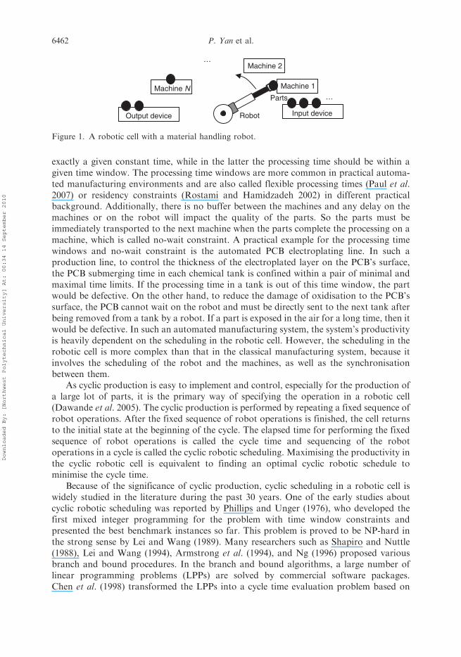
The robotic cell has been a standard tool in modern manufacturing industry, such asprinted circuit board (PCB) electroplating lines, semiconductor manufacturing systems,iron and steel industry, and aircraft manufacturing factories. A typical robotic cell, shownin Figure 1, is composed of an input device, a series of machines, an output device, and amaterial handling robot. The machines are ranged as a semicircle based on the processingtechnology demand. All the parts are available in the input device. They enter the cell fromthe input device, visit each machine successively and finally leave the cell from the outputdevice. A computer-programmed robot transports the parts in the cell. Each robottransporting operation includes: travelling to the machine where the part is located,waiting if necessary, unloading the part, moving the part to the next machine, and loadingthe part. The application of the robotic cell improves the productivity of themanufacturing systems, ensures the quality of the production and reduces the labour cost.

Generally, the part processing times in the robotic cell can be classified into thefixed and time windows. The former means that the processing time on each machine is

*Corresponding author. Email: [email protected]

ISSN 0020–7543 print/ISSN 1366–588X online

� 2010 Taylor & Francis

DOI: 10.1080/00207540903225205

http://www.informaworld.com

Downloaded By: [Northwest Polytechnical University] At: 00:34 14 September 2010

exactly a given constant time, while in the latter the processing time should be within agiven time window. The processing time windows are more common in practical automa-ted manufacturing environments and are also called flexible processing times (Paul et al.2007) or residency constraints (Rostami and Hamidzadeh 2002) in different practicalbackground. Additionally, there is no buffer between the machines and any delay on themachines or on the robot will impact the quality of the parts. So the parts must beimmediately transported to the next machine when the parts complete the processing on amachine, which is called no-wait constraint. A practical example for the processing timewindows and no-wait constraint is the automated PCB electroplating line. In such aproduction line, to control the thickness of the electroplated layer on the PCB’s surface,the PCB submerging time in each chemical tank is confined within a pair of minimal andmaximal time limits. If the processing time in a tank is out of this time window, the partwould be defective. On the other hand, to reduce the damage of oxidisation to the PCB’ssurface, the PCB cannot wait on the robot and must be directly sent to the next tank afterbeing removed from a tank by a robot. If a part is exposed in the air for a long time, then itwould be defective. In such an automated manufacturing system, the system’s productivityis heavily dependent on the scheduling in the robotic cell. However, the scheduling in therobotic cell is more complex than that in the classical manufacturing system, because itinvolves the scheduling of the robot and the machines, as well as the synchronisationbetween them.

As cyclic production is easy to implement and control, especially for the production ofa large lot of parts, it is the primary way of specifying the operation in a robotic cell(Dawande et al. 2005). The cyclic production is performed by repeating a fixed sequence ofrobot operations. After the fixed sequence of robot operations is finished, the cell returnsto the initial state at the beginning of the cycle. The elapsed time for performing the fixedsequence of robot operations is called the cycle time and sequencing of the robotoperations in a cycle is called the cyclic robotic scheduling. Maximising the productivity inthe cyclic robotic cell is equivalent to finding an optimal cyclic robotic schedule tominimise the cycle time.

Because of the significance of cyclic production, cyclic scheduling in a robotic cell iswidely studied in the literature during the past 30 years. One of the early studies aboutcyclic robotic scheduling was reported by Phillips and Unger (1976), who developed thefirst mixed integer programming for the problem with time window constraints andpresented the best benchmark instances so far. This problem is proved to be NP-hard inthe strong sense by Lei and Wang (1989). Many researchers such as Shapiro and Nuttle(1988), Lei and Wang (1994), Armstrong et al. (1994), and Ng (1996) proposed variousbranch and bound procedures. In the branch and bound algorithms, a large number oflinear programming problems (LPPs) are solved by commercial software packages.Chen et al. (1998) transformed the LPPs into a cycle time evaluation problem based on

Machine 1

Robot Input device

Parts

Machine 2

Machine N

Output device

…

…

Figure 1. A robotic cell with a material handling robot.

6462 P. Yan et al.

Downloaded By: [Northwest Polytechnical University] At: 00:34 14 September 2010

bi-valued graphs which can be solved in polynomial time. Lei and Liu (2001) studied arobot processing line which processed two distinct parts and proposed an optimal cyclicscheduling algorithm. Leung et al. (2004) tackled with a multi-robots scheduling problem.They formulated the problem as a mix integer programming and used CPLEX software tosolve it. Geismar et al. (2005) studied the robotic cell with three types of robot travel-timemetrics and developed approximation algorithms to solve the cyclic scheduling problem.

The robotic scheduling problem with fixed processing times, a special case of theproblem with time window constraints attracts the interests of many researchers (see Levneret al. 1997, Kats et al. 1999, Che et al. 2002, Che and Chu 2004, 2007, 2008, Chu 2006, andKats and Levner 2009). They all applied an efficient method called the method of prohibitedintervals (MPI) to formulate the problem and developed several polynomial algorithmsbased on the mathematical analysis of the models. Levner et al. (1997) studied a relativelysimple robotic cyclic scheduling problem where only one part is produced in a cycle. Theyformulated this problem with MPI and developed an O(N3logN) polynomial algorithm,where N is the number of the machines in the cell. Later, using the MPI, Kats et al. (1999),Che et al. (2002), Chu (2006), and Kats and Levner (2009) proposed several polynomialalgorithms for a more general robotic cyclic scheduling problem where two or more partsare produced in each cycle. Che and Chu (2004, 2005, 2007, 2008) tackled two kinds ofmore complex robotic cells, where either complex job flow or multi-robot case is considered.They also used the MPI to formulate the problems and developed some efficient branchand bound approaches to solve these two types of optimal cyclic scheduling problems.

Contrasting the cyclic robotic scheduling problems with time window constraints andthe model with fixed processing times, we find that, if using the MIP, their formulationsare similar in nature, except the processing times are taken as variables in the former, whilethey are constants in the latter. Although many efficient algorithms were developed for theproblems with fixed processing times, to the best of our knowledge, no articles applied theresults of the fixed processing time problem to the problem with time window constraints.In this paper we study an optimal robotic cyclic scheduling problem with processing timewindows, where only one part is produced in a cycle and a single robot is responsible fortransporting parts in the cell. The contributions of this paper are that:

(1) The problem is formulated for the first time as the prohibited intervals of cyclictime by using the MPI. Although the formulated model is similar with the one inLevner et al. (1997), we cannot directly use the method proposed by Levner et al.(1997) to solve the problem. It is because the bounds of the prohibited intervals inour formulation are the linear expression of the processing times while they areconstants in Levner’s.

(2) Based on the mathematical analysis of the formulation, we divided all theprohibited intervals into a series of the subsets and a theorem is presented totransfer our problem into enumerating the non-prohibited intervals of the cycletime in each of the subsets.

(3) An efficient branch and bound algorithm is developed to find the optimal cycletime by enumerating partial non-prohibited intervals. In the search tree, a set ofLPPs are transformed into cycle time evaluation problems which are solved inpolynomial time by a graph-based algorithm.

Note that a similar robotic scheduling problem also exists in more generalmanufacturing cells where the parts are not only allowed to wait on the machine but alsoallowed to wait on a robot for finite or infinite time upon completion of their processing

International Journal of Production Research 6463

Downloaded By: [Northwest Polytechnical University] At: 00:34 14 September 2010

(see Sethi et al. 1992, Ioachim and Soumis 1995, Crama and van de Klundert 1997,Sriskandarajah et al. 1998, Kamoun et al. 1999, Rostami et al. 2001, Rostami andHamidzadeh 2002 and 2004, Kim et al. 2003, Lee and Park 2005, Kim andLee 2008,Wu andZhou 2009). Detailed description and classification of robotic cells scheduling problem canbe found in (Crama et al. 2000, Dawande et al. 2005). Other similar robotic schedulingproblem are studied by Fleury et al. (2001), Lee et al. (2007), Wu and Zhou (2007), Wu et al.(2008), and Gultekin et al. (2008).

This paper is organised as follows. The problem is described and formulated inSection 2. The problem analysis and a branch and bound algorithm are described inSections 3 and 4, respectively. Section 5 gives the computational results. Finally, weconclude the study and discuss future extensions in Section 6.

2. Problem description and formulation

2.1 The problem description

The robotic cell in this study is composed of Nþ 2 machines and a computer controlledrobot. The machines are named as M0,M1, . . . , MN, MNþ1, where M0 and MNþ1 representthe input device and output device respectively. A large lot of identical parts are processedin the robotic cell and each part enters the cell from M0, visits the machines successively asM1, M2, . . . , MN, and finally leaves the cell from MNþ1. A single robot is used to moveparts from one machine to the next one. At any time the machines and the robot canhandle at most one part. The part processing on each machine has a time windowconstraint. The robotic cell adopts simple-cyclic production mode (i.e. in each productioncycle there is exactly one part entering and one part leaving the cell). As soon as a part isunloaded from a machine, it must be transported immediately to the next one. Theproblem in this study is to determine the processing time on each machine with the timewindow constraints so that the cycle time is minimised. To formulate our problem, thefollowing notations are defined:

ai The part minimal processing time on Mi, 1� i�N.bi The part maximal processing time on Mi, 1� i�N.�i The robot move time with a part fromMi toMiþ1, 0� i�N, including:

unloading the part from Mi, moving it to Miþ1 and loading it on Miþ1,which is called move i.

�i,j The robot move time without a part from Mi to Mj, 0� i, j�Nþ 1,and this empty move is called void move.

ti The part processing time on Mi, and must satisfy: ti 2 [ai, bi], 1� i�N,which are decision variables of the problem.

T The cycle time, that is the elapsed time between any two consecutiveparts entering the robotic cell, which is the objective function to beoptimised.

In the remainder of the paper, we call the parts which enter the system at 0, T, 2T , . . . ,as part 0, part 1, part 2 , . . . , respectively. That is to say, the part entering the system at kTis called part k, k� 0. We also make the following assumptions:

�i � �i, iþ1, 0 � i � N, ð1Þ

�i, j � �i, k þ �k, j, 0 � i, j, k � Nþ 1: ð2Þ

6464 P. Yan et al.

Downloaded By: [Northwest Polytechnical University] At: 00:34 14 September 2010

Relation (1) means that a move with a part needs no less time than a move without a

part between the same pair of machines. Relation (2) is commonly known as the triangle

inequality, which imposes our problem into the Euclidean case.

2.2 The problem formulation

We first define intermediate parameters as follows:

si ¼Xij¼1

ð�j�1 þ tj Þ, 1 � i � N: ð3Þ

In this definition, si denotes the completion time of part 0 on Mi, 1� i�N, which is

also the move starting time of part 0 from Mi. Without loss of generality, we set s0¼ 0.

Consequently, kTþ si denotes the completion time of part k on Mi, which is also the move

starting time of part k from Mi, k� 0 and 0� i�N. When the cycle time and the

corresponding processing time on each machine are known, then all the robot move

starting times within [0, T) are determined as follows:

Si ¼ si mode T, 0 � i � N: ð4Þ

We can get the optimal cyclic schedule of the robot moves by sorting all the Si in an

increasing order as follows:

0 ¼ S½0�5S½1�5S½2�5 � � � 5S½ j �5S½ jþ1�5 � � � 5S½N�, ð5Þ

where S[ j ] denotes the starting time of the jth robot moving operation, which means that

the robot moves a part from machine [ j ] to machine [ j ]þ 1 at time: S[j], and after that the

robot moves to machine [ jþ 1] to perform the next operation.A feasible schedule considered in this study must satisfy the following three constraints:

. Machine capacity constraints. For 1� i�N, Mi can process at most one part at

any time.. Robot capacity constraints. The robot can handle at most one part at any time.. Time window constraints. For all the parts and for any 1� i�N, the part

processing time on Mi must fall into the interval [ai, bi].

We give a mathematical formulation of the problem based on the above three

constraints. Note that the first two capacity constraints were formulated by the MPI which

was used for the fixed processing times case in Levner et al. (1997). In our formulation,

we take the processing times as decision variables and exclude some redundant constraints.The machine capacity constraints require that there is no conflict in the use of the

machines between any two parts. Due to the fact that the parts periodically and

successively enter the robotic cell, it is sufficient that there is no conflict in the use of the

machines between any adjacent parts. Consequently, for two adjacent parts, part k and

part kþ 1, k� 0, the previous part k must have been moved out from machine Mi,

1� i�N, when the next part kþ 1, is moved to Mi. We know that the move of part k from

Mi ends at kTþ siþ �i, the move of part kþ 1 from Mi� 1 starts at (kþ 1)Tþ si� 1 and the

void move time from Miþ1 to Mi� 1 is �iþ1,i� 1. Thus, the machine capacity constraints are

International Journal of Production Research 6465

Downloaded By: [Northwest Polytechnical University] At: 00:34 14 September 2010

interpreted as the following intervals forbidden for T:

T =2[Ni¼1

ð�1, si � si�1 þ �i þ �iþ1,i�1Þ: ð6Þ

For the robot capacity constraints, as the robot can handle at most one part at a time,

it must be guaranteed that there is no conflict in the use of the robot between any two

moves. That is to say, for any two moves they cannot be executed at the same time and

furthermore there must be sufficient interval time between the two moves for the robot to

perform the void move. For the move of part kþm from Mj and the move of part k from

Mi, 0� j5 i�N, k� 0, and 1�m� i� j, either the move of part kþm from Mj is

executed earlier than the move of part k from Mi or the former is executed after the latter.

For the first case, we know that the move of part kþm from Mj ends at (kþm) Tþ sjþ �j,the move of part k fromMi starts at kTþ si, and the time for void move fromMjþ1 toMi is

�jþ1,i. The robot capacity for the first case is formulated as:

T � ðsi � sj � �j � �jþ1,iÞ=m, 0 � j5 i � N, and 1 � m � i� j:

Similarly, the robot capacity for the second case is formulated as:

T � ðsi � sj þ �i þ �iþ1, jÞ=m, 0 � j5 i � N, and 1 � m � i� j:

Thus, incorporating the above two relations, we formulate the robot capacity

constraints as the following prohibited intervals for T:

T =2[Ni¼1

[i�1j¼0

[i�jm¼1

ððsi � sj � �j � �jþ1,iÞ=m, ðsi � sj þ �i þ �iþ1,jÞ=mÞ: ð7Þ

In (7), the maximum value of m is i� j. It means that between machine i and machine j,

there are at most i� j parts being processed on the machines.The processing time constraints are formulated as:

ti 2 ½ai, bi�, 1 � i � N: ð8Þ

Additionally, we define:

Qi ¼Xik¼1

tk, 1 � i � N: ð9Þ

With (3) and (9), we have:

si � sj ¼ Qi �Qj þXik¼jþ1

�k�1, 0 � j5 i � N: ð10Þ

Consequently, (6), (7) and (8) can be rewritten respectively by (10) as follows.

T =2[Ni¼1

ð�1,Qi �Qi�1 þ �i�1 þ �i þ �iþ1,i�1Þ, ð11Þ

T =2[Ni¼1

[i�1j¼0

[i�jm¼1

Qi �Qj þXi�1k¼jþ1

�k � �jþ1,i

! ,m, Qi �Qj þ

Xik¼j

�k þ �iþ1,j

!,m

!,

ð12Þ

Qi �Qi�1 2 ½ai, bi�, 1 � i � N: ð13Þ

6466 P. Yan et al.

Downloaded By: [Northwest Polytechnical University] At: 00:34 14 September 2010

Notice that when 1� i�N and j¼ i� 1, the constraints in relation (11) are stricter than

the corresponding part of the constraints in relation (12). The corresponding part of the

intervals in relation (12) with 1� i�N, j¼ i� 1, can be replaced by the intervals inrelation (11). Consequently, a compact formulation is given as follows.

Problem P. Min TSubject to

T =2[Ni¼1

[i�1j¼0

[i�jm¼1

ððQi �Qj þ �i, jÞ=m, ðQi �Qj þ �i, jÞ=mÞ, ð14Þ

Qi �Qi�1 2 ½ai, bi�, 1 � i � N: ð15Þ

The right part of relation (14) is a union of the intervals forbidden for T, and

parameters �i, j and �i, j denote the constants of the left and right bounds of the intervals

respectively. For any pair of i and j, if 1� i�N and j¼ i� 1, then �i,j¼�1,

�i,j¼ �i�1þ �iþ �iþ1,i� 1; for the otherwise, �i, j¼X i�1

k¼jþ1�k � �jþ1,i , �i,j¼

P ik¼j �kþ

�iþ1, j. The intervals in relation (14) are called prohibited intervals for T. If the value of

T falls into one of the prohibited intervals, one of the machines or robot capacity

constraints is violated and this value of T is infeasible for our problem. Contrarily, the

value of T is feasible for our problem. We use W to denote the set of the prohibitedintervals for T in relation (14) as follows.

W ¼ fððQi �Qj þ �i, jÞ=m, ðQi �Qj þ �i, jÞ=mÞ, 0 � j5 i � N, 1 � m � i� jg:

Consequently, solving problem P is searching the minimal value of T which is notcovered by any of the prohibited intervals in W and the constraints (15) are satisfied at the

same time.

3. Problem analysis

It is worthwhile to note that the bounds of intervals in W are linear expressions of the

Qi�Qj, 0� j5 i�N. Both the left and the right bounds increase when Qi�Qj increases,

and vice versa, although the lengths of the intervals do not depend on Qi�Qj. For the sakeof simplicity, in the remainder, we use Em

i, j and Fmi, j to denote the left and right bounds of

the intervals in W. The concise expression of W is:

W ¼ Emi, j, F

mi, j

� �, 0 � j5 i � N, 1 � m � i� j

n o,

where Emi, j � (Qi�Qjþ �i,j)/m and Fm

i, j� (Qi�Qjþ �i, j)/m, for 0� j5 i�N, 1�m� i� j,

and Ei�ji, j 5Ei�j�1

i, j 5 � � �5E2i, j 5E1

i, j and Fi�ji, j 5Fi�j�1

i, j 5 � � �5F 2i, j 5F1

i, j.

We divide W into a set of subsets: wi, j, 0� j5 i�N, as:

W ¼[Ni¼1

[i�1j¼0

wi, j,

where, wi,j¼ {(Ei�ji, j , F

i�ji, j ), (E

i�j�1i, j , Fi�j�1

i, j ), . . . , (E1i, j, F

1i, j)}.

International Journal of Production Research 6467

Downloaded By: [Northwest Polytechnical University] At: 00:34 14 September 2010

Thus, finding a feasible T that does not fall into any intervals in W is equivalent tofinding a value of T that does not fall into any intervals in each of wi, j, 0� j5 i�N. Foreach wi,j, we give in Theorem 1 the conditions under which T is not covered by anyintervals in wi,j.

Theorem 1: For any two adjacent prohibited intervals in wi, j: (Emþ1i, j , Fmþ1

i, j ) and (Emi, j, F

mi, j),

0� j5 i�N and 1�m� i� j� 1, if the condition: Fmþ1i, j � T�Em

i, j is satisfied, then T is notcovered by any prohibited intervals in wi,j.

Proof: See Appendix.According to the Theorem 1, the fact that T cannot be covered by any prohibited

intervals in wi,j is equivalent to guaranteeing that T falls into the non-prohibited intervalbetween a pair of adjacent prohibited intervals in wi,j, 0� j5 i�N. Notice that, any pairof adjacent intervals in wi,j may be disjointed or overlaps with each other. When they aredisjointed, a non-prohibited interval exists between them. Otherwise, no non-prohibitedinterval exists between them. These two cases are shown in Figure 2. However, we cannotknow the relative location of each pair of adjacent intervals in wi,j, since both bounds ofthe intervals are the linear expressions of Qi�Qj and they change as the value of Qi�Qj

changes. We use �wi, j to denote the subset of non-prohibited intervals of T, correspondingto wi,j and construct �wi, j as follows, even though some non-existent non-prohibitedintervals may be involved.

We construct �wi, j as:

�wi, j ¼ C1i, j, D

1i, j

h i, C 2

i, j ,D2i, j

h i, . . . , Ci�j

i, j , Di�ji, j

h in o, 0 � j5 i � N,

where,

C1i, j ¼ �1, D1

i, j ¼ Ei�ji, j , C

2i, j ¼ Fi�j

i, j , D2i, j ¼ Ei�j�1

i, j , . . . ,

Ci�ji, j ¼ F1

i, j and Di�ji, j ¼ þ1, 0 � j5 i � N:

And the Problem P is rewritten as Problem P1.Problem P1. Min TSubject to

T 2 wi, j �[i�jr¼1

Cri, j,D

ri, j

h i, 80 � j5 i � N, ð16Þ

Qi �Qi�1 2 ½ai, bi�, 1 � i � N: ð17Þ

m+1i, jF

m+1i, jF

m+1i, jE m

i, jFmi, jE

mi, jE

……For the first case: ≤

mi, jE

mi, jE

m+1i, jF

m+1i, jF

…m+1i, jE

For the second case: >

…m+1

i, jF

(a)

(b)

.

.

Figure 2. The relative location of two adjacent intervals in wi,j.

6468 P. Yan et al.

Downloaded By: [Northwest Polytechnical University] At: 00:34 14 September 2010

One way to solve Problem P1 consists of enumerating the value of r for each pair of

(i, j ), such that 1� r� i� j and 80� j5 i�N. Since each �wi, j may involve some non-

existent intervals, an efficient branch and bound algorithm is proposed in the rest of the

paper to complete this enumeration. If a non-existent interval in �wi, j is enumerated at some

node in the search tree, no feasible solution can be obtained at this node and this node is

eliminated. For example, suppose [Cri, j,D

ri, j] is a non-existent interval in �wi, j

(i.e., Cri, j 4Dr

i, j), and it is enumerated at node o in the search tree. Since Cri, j 4Dr

i, j,

constraint T2 [Cri, j, D

ri, j] cannot be satisfied and no feasible solution will be obtained at

node o. Accordingly, the procedure eliminates node o and continues to enumerate other

non-prohibited intervals. To illustrate our algorithm, an example is given in advance.Example: A robotic cell is composed of four machines: machine 1, 2, 3 and 4, and the

input device and output device share machine 0. A large lot of identical parts are processed

in this robotic cell. The minimal and maximal processing time limits on the machines 1, 2,

3 and 4 are: [40s, 1000s], [30s, 60s], [30s, 35s], and [20s, 60s] respectively. The time required

to perform the move with a part from machine i to machine iþ 1 (machine 5 is defined to

be machine 0), is (5|i – (iþ 1) mod 5|þ 5)s, i¼ 0, 1, 2, 3, 4. The time for the void move from

machine i to machine j is 5|i – j|s, i and j¼ 0, 1, 2, 3, 4. There is a single robot in the cell and

in each cycle only one part enters and leaves from the cell. For this example, by (14) and

(16), the non-prohibited intervals in each �wi, j are listed in Table 1. In each �wi, j,

0� j5 i�N, the non-prohibited intervals are indexed as: 1, 2, . . . , i� j.In the rest of this section, a definition and another theorem are given, which reduce the

number of non-prohibited intervals to be enumerated in each of �wi, j, 0� j5 i�N. As

analysis at the beginning of this section, the bounds of the intervals in each wi,j,

0� j5 i�N, are linear expressions of Qi�Qj. Meanwhile, each Qi�Qj, 0� j5 i�N, can

be expressed as following form:

Qi �Qj ¼Xik¼jþ1

ðQk �Qk�1Þ, 0 � j5 i � N: ð18Þ

So, the bounds of intervals in each wi,j, 0� j5 i�N, are the linear expression of

Xik¼jþ1

ðQk �Qk�1Þ, 0 � j5 i � N:

Table 1. The non-prohibited intervals for this example.

(i, j) �wi,j

(1, 0) [Q1�Q0þ 15, þ1);(2, 1) [Q2 � Q1þ 30, þ1);(2, 0) (�1, Q2 � Q0þ 5], [Q2� Q0þ 30, þ1);(3, 2) [Q3�Q2þ 30, þ1);(3, 1) (�1, Q3�Q1þ 5], [Q3�Q1þ 45, þ1);(3, 0) (�1, (Q3�Q0þ 10)/2], [(Q3�Q0þ 45)/2, (Q3�Q0þ 10)], [Q3�Q0þ 45, þ1);(4, 3) [Q4�Q3þ 40, þ1);(4, 2) (�1, Q4�Q2þ 5], [Q4�Q2þ 45, þ1);(4, 1) (�1, (Q4�Q1þ 10)/2], [Q4�Q1þ 50)/2, Q4�Q1þ 10], [Q4�Q1þ 50,þ1);(4, 0) (�1, (Q4�Q0þ 15)/3], [Q4�Q0þ 50)/3), (Q4�Q0þ 15)/2],

[(Q4�Q0þ 50)/2, Q4�Q0þ 15], [Q4�Q0þ 50, þ1).

International Journal of Production Research 6469

Downloaded By: [Northwest Polytechnical University] At: 00:34 14 September 2010

Due to the fact that the left bounds of the intervals in �wi, j except the first one (resp.

right bounds of the intervals in �wi, j except the last one) are the right bounds of the intervals

in wi,j (resp. left bounds of the intervals in wi,j), the bounds of intervals in �wi, j, 0� j5 i�N,

are also linear expressions ofPi

k¼jþ1 ðQk �Qk�1Þ. In other words, the bound values of Cri, j

and Dri, j in �wi, j, 1� r� i� j and 0� j5 i�N, both change when any of Qk�Qk� 1,

jþ 1� k� i, changes. If all of Qk�Qk� 1, jþ 1� k� i, are known, then the bounds of the

intervals in �wi, j can be correspondingly determined.

Definition 1: For any 1� r� i� j and 0� j5 i�N, we define the values of Cri, j and Dr

i, j

when Qk�Qk� 1¼ ak, for all jþ 1� k� i, as the min left bound and the min right bound,

denoted as c ri, j and d ri, j.

Theorem 2: For each �wi, j, 0� j5 i�N, the optimal cycle time (denoted as T*), must fall

into one of the non-prohibited intervals, whose min left bounds (i.e. c ri, j’s) are not greater than

the given upper bound of the cycle time (denoted as T 0).

Proof: It is known that the optimal cycle time cannot be greater than the upper bound of

the cycle time, that is:

T � � T 0:

For any interval [Cri, j, D

ri, j] in �wi, j, 1� r� i� j, 1� j5 i�N, if its min left bound, c ri, j, is

greater than the upper bound of cycle time, thus we have:

T � � T 05 c ri, j:

With Definition 1, we know that, for any Qk�Qk� 12 [ak, bk], jþ 1� k� i, c ri, j is the

minimal left bound of [Cri, j, D

ri, j]. That is to say, any other values of Cr

i, j cannot be smaller

than c ri, j. Consequently, we have the following relation:

T � � T 05 c ri, j � Cri, j: ð19Þ

This relation indicates that if the min left bound, c ri, j, is greater than T 0, then it is

impossible that T * falls into [Cri, j,D

ri, j]. Consequently, for each of �wi, j, 0� j5 i�N, the

optimal cycle time must be in one of the non-prohibited intervals whose min left bounds

are not greater than the upper bound of cycle time. œ

Example continued: For this example, T 0 ¼ 120 is an upper bound of cycle time and the

min left and min right bounds in �w4,1 are: c14,1¼�1, d14,1¼ 45, c 24,1¼ 65, d 24,1¼ 90,

c 34,1¼ 130, d 34,1¼þ1. The distribution of these min intervals is presented in Figure 3. The

values of min left bounds: c14,1 and c 24,1 are smaller than T 0, while the other min left bound:

c 34,1 is greater than T 0. Consequently, for the �w4,1, the optimal cycle time can only be found

in the interval: [C14,1, D

14,1] or [C

24,1, D

24,1].

Let pi,j be the number of the non-prohibited intervals in �wi, j, 1� j5 i�N, whose min

left bounds are not greater than T 0. Thus, Theorem 2 means that we only need to

T

14,1 4,1 4,1 4,14,14,1

c = −∞

T' = 120

1d = 45 2c = 65 2d = 903

d = +∞3c = 130

Figure 3. The distribution of the min non-prohibited intervals in the example.

6470 P. Yan et al.

Downloaded By: [Northwest Polytechnical University] At: 00:34 14 September 2010

enumerate the non-prohibited intervals in �wi, j, 1� j5 i�N, whose indices are not greaterthan pi,j, and the non-prohibited intervals whose indices are greater than pi,j are notrequired to be considered.

Note that the initial T 0 can be obtained with LKL algorithm by setting all theQk�Qk� 1¼ ak, for 1� k�N. The detail of the LKL algorithm is referred to Levner et al.(1997). A tighter T 0 can be found at a leaf node of the branch and bound tree, which isdescribed in the next section.

4. Branch and bound algorithm

In what follows, we describe a branch and bound algorithm to enumerate the values of r,(i.e. the indices of the non-prohibited intervals), 1� r� pi,j, for each pair of Qi�Qj, for all0� j5 i�N. For simplifying the description, in the reminder, we use r(i, j ) to denote thevalue of r for each pair of Qi�Qj. Notice that the r(i, j ) are independent; they can bedetermined in any order. Che et al. (2002) tackled a similar enumeration problem whenthey studied an m-cycle robotic scheduling problem with fixed processing times. They gavean empirical enumeration order in their branch and bound algorithm, denoted as CCCalgorithm, which implicitly enumerates the values of r(i, j ) for each pair of Qi�Qj,1� r(i, j )� i� j, 0� j5 i�N. In our study we develop a more efficient enumerationprocedure that could find an optimal solution by only enumerating partial values of r(i, j )for partial pairs of Qi�Qj, 0� j5 i�N.

Before giving our enumeration procedure, it is a prerequisite to briefly describe theCCC algorithm first. With the CCC algorithm, the r(i, j ) enumeration order for ourproblem, denoted as R, is:

R ¼ ðrð1, 0Þ, rð2, 1Þ, rð2, 0Þ, . . . , rðx, x� 1Þ, rðx, x� 2Þ, . . . ,

rðx, 0Þ, . . . , rðN, N� 1Þ, rðN,N� 2Þ, . . . , rðN, 0ÞÞ:

In the search tree, the value of r(1, 0) is first enumerated on the level 1, the values ofr(2, 1) and r(2, 0) are enumerated on the level 2 and level 3 respectively, . . . , and thisenumeration procedure dose not stop until the value of r(N, 0) is enumerated on the(Nþ 1)N/2 level. On each level, the value of r(i, j ) is enumerated as: r(i, j )¼ 1, 2, . . . , i� j,0� j5 i�N. This enumeration process means that the non-prohibited intervals ofQ1�Q0, Q2�Q1, Q2�Q0, . . . , QN�Q0 are enumerated successively from level 1 to level(Nþ 1)N/2 in the search tree. And each node, in the search tree, corresponds to a relaxedproblem of Problem P1. By solving it, we can obtain a relaxed solution to Problem P1, ifthere is the optimal solution for the relaxed problem. And at the leaf node we can obtain afeasible cycle time to Problem P1. The minimal feasible cycle time is the optimal cycle timeto our Problem.

Example continued. For our example, using CCC algorithm, consider a node atlevel 2 in the search tree corresponding to the determined set {r(1, 0)¼ 1, r(2, 1)¼ 1}.Then a relaxed solution can be obtained by solving the following linear programmingproblem:

Min T ð20Þ

Subject to

T 2 ½Q1 �Q0 þ 15, þ1Þ, ð21Þ

International Journal of Production Research 6471

Downloaded By: [Northwest Polytechnical University] At: 00:34 14 September 2010

T 2 ½Q2 �Q1 þ 30, þ1Þ, ð22Þ

Q1 �Q0 2 ½40, 100�, ð23Þ

Q2 �Q1 2 ½30, 60�, ð24Þ

By solving (20)–(24), we get: T¼ 60, and Q0¼ 0, Q1¼ 40, Q2¼ 70. With this relaxed

solution, the non-prohibited intervals of Q2�Q0 in Table 1 are determined as: (�1, 75]and [100, þ1). We find that T¼ 60 is just involved in the first non-prohibited interval

(�1, 75]. It is to say that the relaxed solution obtained by (20)–(24) is feasible for theconstraints of Q2�Q0. Thus, we set r(2, 0)¼ 1 and directly enumerate the value of ther(3, 2). This is because adding the corresponding non-prohibited interval for which

r(2, 0)¼ 1 into (20)–(24) will not change the relaxed solution.Based on the above example, we find that some r(i, j ) are redundant and can be

eliminated if we check the feasibility of the relaxed solution, on each node of the search

tree, using the constraints of those Qi�Qj, whose corresponding r(i, j ) are not enumeratedyet in R. On the other hand, with Theorem 2, we only need to enumerate the non-prohibited intervals in �wi, j whose indices are not greater than pi,j, 0� j5 i�N and we

update the value of pi,j, as soon as a tighter upper bound of T is obtained at a leaf node. Tosum up, for the optimal solution, we can enumerate less values of r(i, j ), 0� j5 i�N.

4.1 A new enumeration procedure

To better understand our enumeration procedure, we use signal ‘/’ to divide R into N sub-orders, that is, R¼ (r(1, 0)/r(2, 1), r(2, 0)/ . . . , /r(x, x� 1), r(x, x� 2), . . . , r(x, 0)/ . . . , /

r(N,N� 1), r(N, N� 2), . . . , r(N, 0)). We call sub-order:/r(x, x� 1), r(x, x� 2), . . . , r(x, 0)/as R(x) for short.

Our new enumeration procedure includes two layers. The upper layer is about the sub-order’s enumeration order, which indicates that R(1),R(2), . . . ,R(N) are enumerated

successively. The lower layer enumerates the r(i, j ) for each given sub-order, where wecheck the feasibility of the relaxed solution before enumerating r(i, j ).

As we know, any node in the search tree corresponds to a set of r(i, j ), whose values aredetermined. For example, node o in the search tree corresponds to the set {r(1, 0),

r(2, 1), . . . , r(x, j), 0� j5 x�N}, denoted as �(o), whose values of r(i, j ) are determined.With the determined values of these r(i, j ) in �(o), a relaxed problem to Problem P1 can be

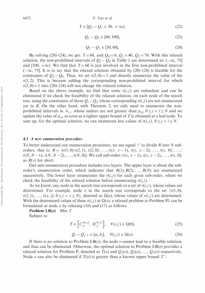
formulated at node o by relaxing (16) and (17) as follows.Problem LB(o) Min TSubject to

T 2 Crði, j Þi, j , D

rði, j Þi, j

h i, 8 ði, j Þ 2 �ð0Þ, ð25Þ

Qi �Qi�1 2 ½ai, bi�, 8ði, j Þ 2 �ðoÞ: ð26Þ

If there is no solution to Problem LB(o), the node o cannot lead to a feasible solution,and thus can be eliminated. Otherwise, the optimal solution to Problem LB(o) provides arelaxed solution for Problem P, denoted as T(o) and Q1(o), Q2(o), . . . , Qx(o) respectively.

Node o can also be eliminated if T(o) is greater than a known upper bound T 0.

6472 P. Yan et al.

Downloaded By: [Northwest Polytechnical University] At: 00:34 14 September 2010

Notice that, in �(o), R(x) is the latest enumerated sub-order and r(x, j) is the latest one

enumerated in R(x). For the rest of r(x, y) in R(x), 0� y5 j, which have not been

enumerated, we find that to enumerate r(x, y) is just to add the non-prohibited interval of

Qx�Qy into Problem LB(o). Due to the fact that the values of Qx(o) �Qy(o) may lead one

of the non-prohibited intervals of Qx�Qy involves T(o), that is to say, if it happens, to add

this non-prohibited interval into Problem LB(o) and to re-solve the Problem LB(o) have

no contribution to finding the optimal cycle time. Consequently, before enumerating the

rest of r(x, y) in R(x), 0� y5 j5 x, we first check the feasibilities of T(o) with the

non-prohibited intervals of Qx – Qy, 0� y5 j5 x. If there exists at least one pair of

Qx – Qy, such that T(o) does not fall into any of the non-prohibited intervals determined

by Qx(o) – Qy(o), then the branching from node o is to enumerate the non-prohibited

intervals of Qx – Qy and r(x, y) is accordingly added to �(o). If a pair of Qx – Qy, such that

T(o) falls into one of the non-prohibited intervals determined by Qx(o) – Qy(o), then set the

value of r(x, y) as the index of the non-prohibited interval where T(o) falls and add r(x, y)

to �(o). This process continues until for any pair of (x, y) such that 0� y5 j, T(o) falls

into its non-prohibited intervals. When this process finishes, we turn to enumerate all the

pairs of (i, j ) in the sub-order R(xþ 1). To achieve this, r(xþ 1, x) is first enumerated.

Accordingly, r(xþ 1, x) is added into �(o). The enumeration process of the rest of

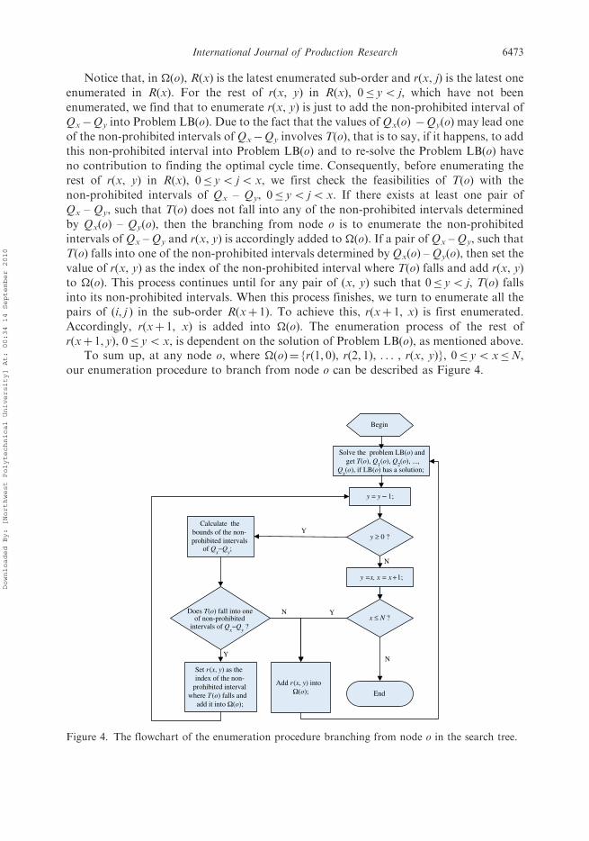
r(xþ 1, y), 0� y5 x, is dependent on the solution of Problem LB(o), as mentioned above.To sum up, at any node o, where �(o)¼ {r(1, 0), r(2, 1), . . . , r(x, y)}, 0� y5 x�N,

our enumeration procedure to branch from node o can be described as Figure 4.

y = y – 1;

y ≥ 0 ?

Calculate the bounds of the non-prohibited intervals

of Qx−Q

y;

Does T(o) fall into one of non-prohibited

intervals of Qx−Q

y ?

Set r(x, y) as the index of the non-

prohibited interval where T(o) falls and

add it into Ω(o);

Add r(x, y) into Ω(o);

y =x, x = x +1;

x ≤ N ?

End

N

Y

N

Y

Begin

N

Y

Solve the problem LB(o) and get T(o), Q1(o), Q2(o), ...,

Qx(o), if LB(o) has a solution;

Figure 4. The flowchart of the enumeration procedure branching from node o in the search tree.

International Journal of Production Research 6473

Downloaded By: [Northwest Polytechnical University] At: 00:34 14 September 2010

In this enumerate procedure, all the r(x, x – 1), 1� x�N, are first enumerated in eachsub-order. However, the rest of r(x, y), 0� y5 x – 1, that need to be enumerated are basedon the relaxed solution of Problem LB(o). It implies that the shortest enumeration order is:(r(1, 0)/r(2, 1/ . . . , /r(x, x� 1)/ . . . , /r(N, N� 1)) and the longest enumeration order is thesame as CCC’s enumeration order (i.e. R).

4.2 Solving the problem LB(o)

To solve Problem LB(o), the equivalent expression of Problem LB(o) is given as follows.Problem LB0(o) Min TSubject to

mT� �i, j � Qi �Qj � ðmþ 1ÞT� �i,j, 8 ði, j Þ 2 �ðoÞ, 1 � m � pi, j, ð27Þ

ai � Qi �Qi�1 � bi, 1 � i � N: ð28Þ

Because of its special structure, Problem LB0(o) can be transformed into a cycle timeevaluation problem in a bi-valued graph and it can be solved in polynomial time. Pleasesee Chen et al. (1998) and Che et al. (2002) for details.

4.3 Search strategy

In the branch and bound algorithm, we use the depth-first plus best lower bound rule toselect the node for the next branching. A feasible cycle time is obtained at a leaf node. Ifthe feasible cycle time is tighter than the known upper bound, then we update the upperbound as this feasible cycle time and correspondingly update the value of pi,j, for0� j5 i�N with Theorem 2. The minimal feasible cycle time at the leaf nodes is theoptimal cycle time (i.e. T * ). And with its corresponding feasible solution, Q1, Q2, . . . , QN,the optimal processing times on each machine are calculated as follows:

ti ¼ Qi �Qi�1, 1 � i � N, where Q0 ¼ 0: ð29Þ

The corresponding robot move starting times within [0, T) are determined by (4). Byordering these move starting times in increasing order as (5), an optimal cyclic schedulingin the robotic cell is obtained.

Example continued. The search tree for the example is presented in Figure 5. In thisfigure, sign ‘’ denotes the node in the tree that has a relaxed solution, sign ‘’ denotes thenode that does not have the solution and sign ‘�’ denotes that the relaxed solution obtainedat its father node is feasible for this node and Problem LB(o) is not solved at this node. In thesearch tree, for example, node r(3,0)¼ 3 is a ‘�’, that is because the relaxed solution:Q0¼ 0,Q1¼ 70, Q2¼ 100, Q3¼ 130, T¼ 105, obtained at its father node r(3,1)¼ 2, leads the valueof T to fall into the non-prohibited interval [Q3 – Q0þ 45, þ1). Thus, we just set r(3,0)¼ 3and branch from this node to enumerate the others. Using our branch and bound approach,the optimal solution is obtained in the leaf node ‘�’ in the search tree by solving the ProblemP defined by: (r(1, 0)¼ 1/r(2, 1)¼ 1, r(2, 0)¼ 1/r(3, 2)¼ 1, r(3, 1)¼ 2/r(4, 3)¼ 1, r(4, 1)¼ 2).Therefore the optimal cycle time is: T *¼ 110, with Q1¼ 70, Q2¼ 105, Q3¼ 135, Q4¼ 170,and the corresponding processing time for machine 1, 2, 3 and 4 are: t1¼ 70, t2¼ 35, t3¼ 30,and t4¼ 35, respectively. Correspondingly, by (3), the completion time of part 0 on Mi,

6474 P. Yan et al.

Downloaded By: [Northwest Polytechnical University] At: 00:34 14 September 2010

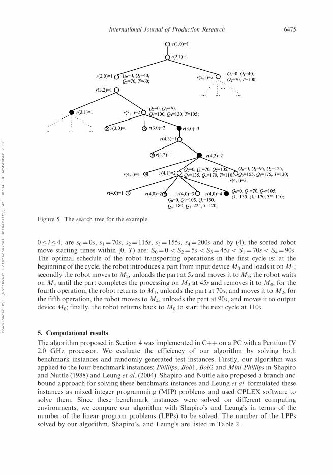
0� i� 4, are s0¼ 0s, s1¼ 70s, s2¼ 115s, s3¼ 155s, s4¼ 200s and by (4), the sorted robotmove starting times within [0, T) are: S0¼ 05S2¼ 5s5S3¼ 45s5S1¼ 70s5S4¼ 90s.The optimal schedule of the robot transporting operations in the first cycle is: at thebeginning of the cycle, the robot introduces a part from input deviceM0 and loads it onM1;secondly the robot moves toM2, unloads the part at 5s and moves it toM3; the robot waitson M3 until the part completes the processing on M3 at 45s and removes it to M4; for thefourth operation, the robot returns to M1, unloads the part at 70s, and moves it to M2; forthe fifth operation, the robot moves to M4, unloads the part at 90s, and moves it to outputdevice M0; finally, the robot returns back to M0 to start the next cycle at 110s.

5. Computational results

The algorithm proposed in Section 4 was implemented in Cþþ on a PC with a Pentium IV2.0 GHz processor. We evaluate the efficiency of our algorithm by solving bothbenchmark instances and randomly generated test instances. Firstly, our algorithm wasapplied to the four benchmark instances: Phillips, Bob1, Bob2 and Mini Phillips in Shapiroand Nuttle (1988) and Leung et al. (2004). Shapiro and Nuttle also proposed a branch andbound approach for solving these benchmark instances and Leung et al. formulated theseinstances as mixed integer programming (MIP) problems and used CPLEX software tosolve them. Since these benchmark instances were solved on different computingenvironments, we compare our algorithm with Shapiro’s and Leung’s in terms of thenumber of the linear program problems (LPPs) to be solved. The number of the LPPssolved by our algorithm, Shapiro’s, and Leung’s are listed in Table 2.

Figure 5. The search tree for the example.

International Journal of Production Research 6475

Downloaded By: [Northwest Polytechnical University] At: 00:34 14 September 2010

Note that the last instance Min Phillips was constructed by Leung in 2004, which is thetruncation of the Phillips to the first nine machines. So, we cannot know the number ofLPPs solved for this instance by Shapiro’s. Comparing the data in Table 2, we find thatour algorithm solved less LPPs than Shapiro’s for the first three instances and solved lessLPPs than the Leung’s for the instances: Phillips, Bob1 and Min Phillips, except the Bob2.Our algorithm’s improvement rates on the number of LPPs compared with Shapiro’s are:29%, 66%, 45% and N/A and with Leung’s are: 96%, 12%, �7%, and 87%. For theBob2, the LPPs solved by ours are 7% more than Leung’s. It is because, in our branch andbound approach, we use the depth-first plus best lower bound rule to select the node forthe next branching. This search strategy has a greed nature and is efficient in most cases.However, for the Bob2, a special case, if we adopt breadth-first plus best lower bound ruleto select the node, we will find that the number of the LPPs solved is much less than that ofLeung’s. On the other hand, 1800 stochastic test instances were generated to evaluate theperformance of the algorithm. All the test instances were generated with a random numberstream. Let U(c1, c2) denote a positive integer randomly drawn from a uniformdistribution with lower and upper bounds c1 and c2, respectively. Parameters used togenerate the instances were:

ai ¼ Uð20, 100Þ, �i,iþ1 ¼ �i,iþ1 ¼ Uð0, 2Þ, �i, j ¼ �j,i ¼Xj�1k¼i

�k,kþ1,

�i ¼ �i,iþ1 þ 2, 0 � i5 j � Nþ 1, N 2 f6, 8, 10, 12, 14, 16g:

In addition, we set Dp¼ {0.2, 0.4, 0.6}, which represents the range rate between theminimal and maximal processing times, i.e. Dp¼ 2(bi� ai)/(biþ ai), and then bi¼ ai(2þDp)/(2�Dp). For each given pair of (N, Dp), 100 random instances were generated.

The average CPU computation times and the average number of LPPs solved for eachpair of parameters (N, Dp) are listed in Table 3. The data in Table 3 indicate that as thenumber of machines (i.e. N) increases, the average computation times show an exponentialincreasing trend. However, as the range rate of time window (i.e. Dp) increases, the averagecomputation times show a linear increasing trend. Besides that, the data show that theaverage computation times have the same increasing trend with the average number ofLPPs solved. It is because in our algorithm, the computation time for each test mainlydepends on the number of LPPs solved and the computation time for solving each LPP. Asdescribed above, the LPP is solved in polynomial time by a graph-based algorithm, so theaverage computation times have the same increasing trend with the average number ofLPPs solved.

For further testing of the efficiency of the algorithm, we compared our newenumeration order (NEO) with the old enumeration order in CCC algorithm (CCC)

Table 2. The computational results of benchmark instances.

Instances Number of machines

Number of LPPs solved by . . .

Our algorithm Shapiro’s algorithm Leung’s algorithm

Phillips 13 2058 2896 49,321Bob1 12 1364 3985 1547Bob2 12 10,988 19,873 10,295Min Phillips 9 76 N/A 583

6476 P. Yan et al.

Downloaded By: [Northwest Polytechnical University] At: 00:34 14 September 2010

which is mentioned in Section 4. The percentages of the average computation times withNEO to that with CCC and the percentages of average number of LPPs solved by NEO tothat solved by CCC for the same random instances are listed in Table 4. Observing thedata in Table 4, it shows clearly that percentages of the average computation times withNEO to that with CCC are all smaller than 100% (the minimal percentage is 44.45% andthe maximal percentage is 87.14%), which implies that the computation times with NEOare less than that with CCC, for all the pairs of parameters (N, Dp). That is becausethe number of LPPs solved by NEO is less than that solved by CCC, which is provedby the percentages of average number of LPPs solved by NEO to that solved by CCCin Table 4 (the minimal percentage is 41.55%, and the maximal percentage is 84.79%).To sum up, it shows that our algorithm is more efficient to solve this problem.

6. Conclusion

The result of this study provides another way to solve the cyclic robotic schedulingproblem with time window constraints. The problem is to decide the processing time oneach machine to minimise the cycle time. We formulate this problem as the fixedprocessing problem based on the notion of prohibited intervals of cycle time, and it is

Table 4. The percentage of the average computation times of NEO/CCC and the percentage ofaverage number of LPPs solved of NEO/CCC.

N

Dp¼ 0.2 Dp¼ 0.4 Dp¼ 0.6

AverageCPU time LPPs solved

AverageCPU time LPPs solved

AverageCPU time LPPs solved

6 63.00% 48.38% 50.00% 41.55% 44.45% 42.89%8 50.00% 67.58% 60.47% 62.53% 83.02% 84.79%10 68.52% 60.14% 64.68% 62.27% 87.14% 83.84%12 49.68% 57.65% 67.47% 53.62% 67.34% 69.16%14 56.12% 45.63% 72.37% 62.09% 75.37% 61.43%16 48.55% 51.32% 48.85% 47.45% 78.54% 67.81%

Table 3. Average computation times and average number of LPPs solved by our algorithm.

N

Dp¼ 0.2 Dp¼ 0.4 Dp¼ 0.6

AverageCPU time(second)

Averagenumber ofLPPs solved

AverageCPU time(second)

Averagenumber ofLPPs solved

AverageCPU time(second)

Averagenumber ofLPPs solved

6 0.001 31 0.004 77 0.009 1528 0.006 145 0.043 638 0.106 130610 0.054 567 0.252 3123 1.120 680712 0.316 2031 0.704 7193 2.143 12,94114 4.690 23,125 6.891 45,631 9.348 52,43716 25.652 305,432 75.872 325,785 234.871 894,684

International Journal of Production Research 6477

Downloaded By: [Northwest Polytechnical University] At: 00:34 14 September 2010

transformed into the enumeration of the non-prohibited intervals for the optimal cycletime. This enumeration is completed by a branch and bound algorithm with a moreefficient enumeration order. As both bounds of the non-prohibited intervals are linearexpressions of the processing times, the relaxed problem at each node of the search tree issolved by a cycle time evaluation method based on bi-valued graphs. The performance ofthe algorithm was evaluated by benchmark instances and 1800 randomly generatedinstances. The computational results indicate that the proposed algorithm is efficient. Theresult of this study could be extended to more complex scheduling problems in robotic cellswhere multi-type of parts are processed or two or more robots are used.

Acknowledgements

This work was partially supported by the National Natural Science Foundation of China underGrant No. 50605052 and the Program for New Century Excellent Talents in Universities of Ministryof Education, China, under Grant No. NCET-06-0875.

References

Armstrong, R., Lei, L., and Gu, S., 1994. A bounding scheme for deriving the minimal cycle time ofa single transporter N-stage process with time windows. European Journal of Operational

Research, 78 (1), 224–227.Che, A. and Chu, C., 2004. Single-track multi-hoist scheduling problem: a collision-free resolution

based on a branch and bound approach. International Journal of Production Research, 42 (12),

2435–2456.Che, A. and Chu, C., 2005. Multi-degree cyclic scheduling of two robots in a no-wait flowshop.

IEEE Transactions on Automation Science and Engineering, 2 (2), 173–183.

Che, A. and Chu, C., 2007. Cyclic hoist scheduling in large real-life electroplating lines. ORSpectrum, 29 (3), 445–470.

Che, A. and Chu, C., 2008. Optimal scheduling of material handling devices in a PCB productionline: problem formulation and a polynomial algorithm. Mathematical Problems inEngineering, Article ID 364279, 21.

Che, A., Chu, C., and Chu, F., 2002. Multicyclic hoist scheduling with constant processing times.IEEE Transactions on Robotics and Automation, 18 (1), 69–80.

Chen, H., Chu, C., and Proth, J.-M., 1998. Cyclic scheduling of a hoist with time window

constraints. IEEE Transactions on Robotics and Automation, 14 (1), 144–152.Chu, C., 2006. A faster polynomial algorithm for 2-cyclic robotic scheduling. Journal of Scheduling,

9 (5), 435–468.

Crama, Y. and van de Klundert, J., 1997. Cyclic scheduling of identical parts in a robotic cell.Operational Research, 45 (6), 952–965.

Crama, Y., et al., 2000. Cyclic scheduling in robotic flowshops. Annals of Operations Research,

96 (1–4), 97–124.Dawande, M., et al., 2005. Sequencing and scheduling in robotic cells: Recent developments. Journal

of Scheduling, 8/5, 387–426.

Fleury, G., Gourgand, M., and Lacomme, P., 2001. Metaheuristics for the stochastic hoistscheduling problem (SHSP). International Journal of Production Research, 39 (15),

3419–3457.Geismar, H.N., Dawande, M., and Sriskandarajah, C., 2005. Approximation algorithms for k-

unit cyclic solutions in robotic cells. European Journal of Operational Research, 162 (2),

291–309.

6478 P. Yan et al.

Downloaded By: [Northwest Polytechnical University] At: 00:34 14 September 2010

Gultekin, H., Akturk, M.S., and Karasan, O.E., 2008. Scheduling in robotic cells: process flexibility

and cell layout. International Journal of Production Research, 46 (8), 2105–2121.

Ioachim, I. and Soumis, F., 1995. Schedule efficiency in a robotic production cell. International

Journal of Flexible Manufacturing Systems, 7 (1), 5–26.

Kamoun, H., Hall, N.G., and Sriskandarajah, C., 1999. Scheduling in robotic cells: Heuristic and

cell design. Operational Research, 47 (6), 821–835.

Kats, V., Levner, E., and Meyzin, L., 1999. Multiple-part cyclic hoist scheduling using a sieve

method. IEEE Transactions on Robotics and Automation, 15 (4), 704–713.

Kats, V. and Levner, E., 2009. A polynomial algorithm for 2-cyclic robotic scheduling:

a non-Euclidean case. Discrete Applied Mathematics, 157 (2), 339–355.

Kim, J. and Lee, T., 2008. Schedulability analysis of time-constrained cluster tools with bounded

time variation by an extended Petri net. IEEE Transactions on Automation Science and

Engineering, 5 (3), 490–503.Kim, J., et al., 2003. Scheduling of dual-armed cluster tools with time constraints. IEEE Transactions

on Semiconductor Manufacturing, 16 (3), 521–534.Lei, L. and Wang, T.J., 1989. A proof: the cyclic hoist scheduling problem is NP-hard. Working

Paper #89–0016. Rutgers University.Lei, L. and Liu, Q., 2001. Optimal cyclic scheduling of a robotic processing line with two-product

and time-window constraints. INFOR, Information Systems and Operational Research, 39 (2),

185–199.Lee, T.E., Lee, H.Y., and Lee, S.J., 2007. Scheduling a wet station for wafer cleaning with multiple

job flows and multiple wafer-handling robots. International Journal of Production Research,

45 (3), 487–507.

Lee, T.E. and Park, S., 2005. An extended event graph with negative places and negative tokens for

time window constraints. IEEE Transactions on Automation Science and Engineering, 2 (4),

319–332.Levner, E., Kats, V., and Levit, V., 1997. An improved algorithm for cyclic scheduling in a robotic

cell. European Journal of Operational Research, 97, 500–508.Leung, J.M.-Y., et al., 2004. Optimal cyclic multi-hoist scheduling: A mixed integer programming

approach. Operations Research, 52 (6), 965–976.Ng, W.C., 1996. A branch and bound algorithm for hoist scheduling of a circuit board production

line. International Journal of Flexible Manufacturing Systems, 8 (1), 45–65.Paul, H.J., Bierwirth, C., and Kopfer, H., 2007. A heuristic scheduling procedure

for multi-item hoist production lines. International Journal of Production Economics,

105 (1), 54–69.Phillips, L. and Unger, P., 1976. Mathematical programming solution of a hoist scheduling program.

IIE Transactions, 8 (2), 219–225.Rostami, S. and Hamidzadeh, B., 2002. Optimal scheduling techniques for cluster tools with process

module and transport-module residency constraints. IEEE Transactions on Semiconductor

Manufacturing, 15 (3), 341–349.Rostami, S. and Hamidzadeh, B., 2004. An optimal residency-aware scheduling technique for

cluster tools with buffer module. IEEE Transactions on Semiconductor Manufacturing,

17 (1), 68–73.

Rostami, S., Hamidzadeh, B., and Camporese, D., 2001. An optimal periodic scheduler for dual arm

robots in cluster tools with residency constraints. IEEE Transactions on Robotics and

Automation, 17 (5), 609–618.Sethi, S.P., et al., 1992. Sequencing of parts and robot moves in a robotic cell. International Journal

of Flexible Manufacturing Systems, 4/3 (4), 331–358.Shapiro, G. and Nuttle, H., 1988. Hoist scheduling for a part electroplating facility. IIE

Transactions, 20 (2), 157–167.

International Journal of Production Research 6479

Downloaded By: [Northwest Polytechnical University] At: 00:34 14 September 2010

Sriskandarajah, C., Hall, N.G., and Kamoun, H., 1998. Scheduling large robotic cells without

buffers. Annals of Operations Research, 76, 287–321.

Wu, N., et al., 2008. A Petri net method for schedulability and scheduling problems in single–arm

cluster tools with wafer residency time constraints. IEEE Transactions on Semiconductor

Manufacturing, 21 (2), 224–237.Wu, N. and Zhou, M., 2007. Deadlock modeling and control of semiconductor track systems using

resource-oriented Petri nets. International Journal of Production Research, 45 (15), 3439–3456.Wu, N. and Zhou, M., 2009. A closed-form solution for schedulability and optimal scheduling

of dual–arm cluster tools with wafer residency time constraint based on steady schedule

analysis. IEEE Transactions on Automation Science and Engineering, DOI: 10.1109/

TASE.2008.200865,2009.

Appendix

Proof of Theorem 1: By definition, intervals (Emþ1i, j , Fmþ1

i, j ) and (Emi, j, F

mi, j) are adjacent intervals in

wi, j and we have the following relations:

Emþ1i, j 5Em

i, j 5Fmi, j, 1 � m � i� j� 1 and 0 � j5 i � N: ðaÞ

Emþ1i, j 5Fmþ1

i, j 5Fmi, j, 1 � m � i� j� 1 and 0 � j5 i � N: ðbÞ

If the value of T satisfies the condition: Fmþ1i, j �T�Em

i, j, we have the following relation:

Fi�ji, j 5 � � � 5Fmþ2

i, j 5Fmþ1i, j � T � Em

i, j 5Em�1i, j 5 � � � 5E1

i, j:

This relation implies that, for any k such that mþ 1� k� i� j, T is greater than the right boundof interval (Ek

i, j, Fki, j), namely, T is not involved in these intervals in wi, j; and for any l such that

1� l�m, T is smaller than the left bound of interval (Eli, j, F

li, j), namely, T is not involved in these

intervals either. Consequently, for a given m, 1�m� i� j� 1, if Fmþ1i, j �T�Em

i, j, then T is notcovered by any intervals in wi, j. œ

6480 P. Yan et al.

Downloaded By: [Northwest Polytechnical University] At: 00:34 14 September 2010