A Bounded Index Test to Make Robust Heterogeneous Welfare Comparisons

A Bounded Index Test to make Robust Heterogeneous Welfare Comparisons by André DECOSTER Erwin OOGHE Public Economics Center for Economic Studies Discussions Paper Series (DPS) 05.05 http://www.econ.kuleuven.be/ces/discussionpapers/default.htm

January 2005

A bounded index test to make robust heterogeneous

welfare comparisons.∗

André Decoster and Erwin OogheCES, Katholieke Universiteit Leuven†

January, 2005

Abstract

Fleurbaey, Hagneré and Trannoy (2003) develop a bounded dominance test to makerobust welfare comparisons, which is intermediate between Ebert’s (1999) cardinal

dominance criterion –generalized Lorenz dominance applied to household incomes,divided and weighted by an equivalence scale– and Bourguignon’s (1989) ordinaldominance criterion. In this paper, we develop a more complete, but less robustbounded index test, which is intermediate between Ebert’s (1997) cardinal indextest –an index applied to household incomes, divided and weighted by the equiv-alence scale– and a (new) sequential index test –an index applied to householdincomes of the most needy only, the most and second most needy only, and so on.We illustrate the power of our test to detect welfare changes in Russia using dataof the RLMS-surveys.

1 Introduction

When income units are homogeneous in non-income characteristics, there exist many

tools to evaluate income distributions and the properties of these tools are well-known;

see Lambert (2001) for an overview. Basically, these tools can be classified in two groups.

Indices map income distributions into a comparable number measuring the welfare of

the distribution under consideration, whereas dominance criteria look for unanimity

among a “wide” class of such indices. The most well-known dominance criterion is the

generalized Lorenz dominance (GLD) criterion due to Shorrocks (1983). Unfortunately,

these tools are not well-suited to make reasonable comparisons in practice, because “At

∗We are grateful to Bart Capéau, Peter Lambert and Luc Lauwers for useful comments and help.†Center for Economic Studies, Katholieke Universiteit Leuven, Naamsestraat, 69, B-3000 Leu-

ven, Belgium. André Decoster is Professor of Economics. e-mail to andré[email protected].

Erwin Ooghe is a Postdoctoral Fellow of the Fund for Scientific Research - Flanders. e-mail to

[email protected].

1

the heart of any distributional analysis, there is the problem of allowing for differences

in people’s non-income characteristics” (Cowell and Mercader-Prats (1999)).

To make robust heterogeneous welfare comparisons, the most well-known result is Atkin-

son and Bourguignon’s (1987) sequential generalized Lorenz dominance (SGLD) crite-

rion: (i) divide all income units into different need types on the basis of non-income

characteristics and (ii) check –on the basis of the GLD criterion– whether the most

needy in one distribution dominate the most needy in another distribution, whether

the most and second most needy together in the former distribution also dominate the

most and second most needy in the other distribution, and so on. The SGLD criterion

is very robust –as it is equivalent to unanimity among a wide set of utilitarian welfare

orderings– but it has little power to rank distributions. It has been extended by Atkin-

son (1992), Jenkins and Lambert (1993), Chambaz and Maurin (1998), Lambert and

Ramos (2002), and Moyes (1999) to deal with changing demographics, poverty and/or

the principle of diminishing transfers. We also refer to Bourguignon (1989) for a related

dominance criterion.

The SGLD criterion is often called an “ordinal” dominance criterion, because the needs

classes have to be defined in an ordinal way only, i.e., a ranking of all non-income types

on the basis of needs. In contrast, practitioners often use equivalence scales to cardinalize

needs differences between income units, expressing, e.g., that (for each income level) a

couple needs m times the income of a single to reach the same living standards, with m

between 1 and 2. Equivalence scales are defined with respect to a reference type, usually

a single. Once defined, practitioners can (i) transform the heterogeneous distribution of

incomes and types into a homogeneous distribution of equivalent incomes (for reference

types) and (ii) use a standard tool (an index or dominance criterion) applied to the

vector of equivalent incomes. Depending on the chosen tool, we call it either a cardinal

index or a cardinal dominance approach.1

Fleurbaey, Hagneré and Trannoy (2003) consider a dominance criterion which is inter-

mediate between the ordinal and the cardinal approach. They propose to make welfare

comparisons using the GLD criterion for a bounded set of equivalence scale vectors.

Choosing the bounded set as small as possible, their criterion reduces to Ebert’s (1999)

cardinal GLD approach –the GLD criterion applied to household incomes, both divided

and weighted by the (unique) equivalence scale– and choosing the bounded set as wide

as possible, their criterion is equivalent with one of Bourguignon’s (1989) dominance

criteria.

The different existing ways to deal with heterogeneity, as well as the main contributions,1As noted by Pyatt (1990) and Glewwe (1991), the use of an equivalence scale may give rise to

a weighting problem. More precisely, it is not clear whether one should weight each income unit by

the number of individuals or by the equivalence scale; see Ebert (1997), Ebert and Moyes (2003) and

Shorrocks (2005), and Capéau and Ooghe (2004) for a possible solution.

2

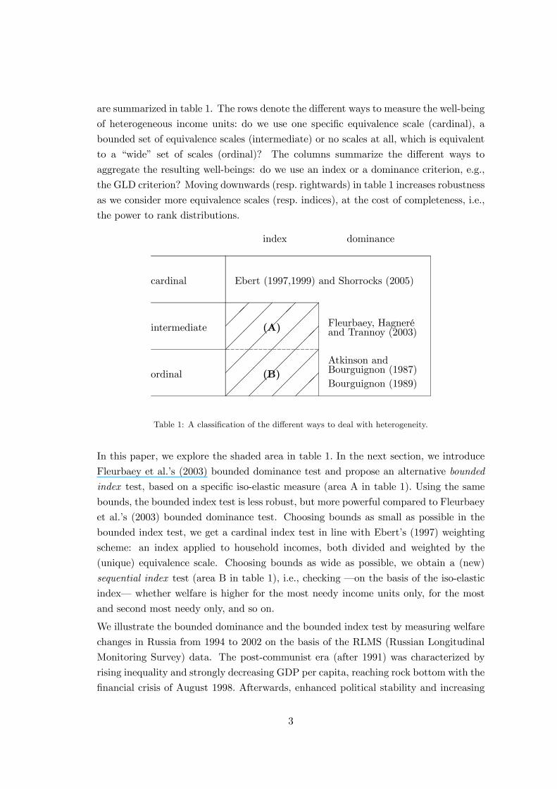
are summarized in table 1. The rows denote the different ways to measure the well-being

of heterogeneous income units: do we use one specific equivalence scale (cardinal), a

bounded set of equivalence scales (intermediate) or no scales at all, which is equivalent

to a “wide” set of scales (ordinal)? The columns summarize the different ways to

aggregate the resulting well-beings: do we use an index or a dominance criterion, e.g.,

the GLD criterion? Moving downwards (resp. rightwards) in table 1 increases robustness

as we consider more equivalence scales (resp. indices), at the cost of completeness, i.e.,

the power to rank distributions.

cardinal

intermediate

ordinal

index dominance

Ebert (1997,1999) and Shorrocks (2005)

Fleurbaey, Hagneréand Trannoy (2003)

Atkinson andBourguignon (1987)Bourguignon (1989)

(A)

(B)

Table 1: A classification of the different ways to deal with heterogeneity.

In this paper, we explore the shaded area in table 1. In the next section, we introduce

Fleurbaey et al.’s (2003) bounded dominance test and propose an alternative bounded

index test, based on a specific iso-elastic measure (area A in table 1). Using the same

bounds, the bounded index test is less robust, but more powerful compared to Fleurbaey

et al.’s (2003) bounded dominance test. Choosing bounds as small as possible in the

bounded index test, we get a cardinal index test in line with Ebert’s (1997) weighting

scheme: an index applied to household incomes, both divided and weighted by the

(unique) equivalence scale. Choosing bounds as wide as possible, we obtain a (new)

sequential index test (area B in table 1), i.e., checking –on the basis of the iso-elastic

index– whether welfare is higher for the most needy income units only, for the most

and second most needy only, and so on.

We illustrate the bounded dominance and the bounded index test by measuring welfare

changes in Russia from 1994 to 2002 on the basis of the RLMS (Russian Longitudinal

Monitoring Survey) data. The post-communist era (after 1991) was characterized by

rising inequality and strongly decreasing GDP per capita, reaching rock bottom with the

financial crisis of August 1998. Afterwards, enhanced political stability and increasing

3

oil prices led to strong growth and slowly decreasing inequality. Therefore, we expect

welfare to decrease in the first and to rise again in the second period. While the bounded

index test is able to detect such a pattern, this is not the case for the bounded dominance

test. Robustness with respect to the aggregation of well-beings, rather than with respect

to its measurement, turns out to be the main culprit.

2 Robust welfare comparisons

2.1 Notation

Consider household incomes y ∈ R+ and types k ∈ K = {1, ...,K} representing relevantnon-income characteristics; types are ordered from least (k = 1) to most needy (k = K).

A heterogeneous distribution is denoted by F = (p1, ..., pK , F1, ..., FK), with pk the

proportion of households with type k and Fk the (differentiable) income distribution

function of type k households defined over R+ with a finite support [0, sk]. We focusdirectly on the case where demographics might change, or the proportions pk may vary

over the different distributions. Household utility functions Uk : R+ → R measure theutility of a household with type k as a function of its income, with Uk (0) finite for all

k ∈ K. Social welfare in a distribution F is measured by the average household utility

in society:

W : F →W (F ) =k∈K

pksk

0UkdFk. (1)

2.2 A bounded dominance test

Fleurbaey, Hagneré and Trannoy (FHT in the sequel) consider a lower and upper bound

vector α,β ∈ RK which satisfy

(1, 1, . . . , 1) ≤ (α1 = 1,α2, . . . ,αK) ≤ (β1 = 1,β2, . . . ,βK) . (2)

Type 1 (the least needy type) will be referred to as the reference type. They impose the

following conditions on household utility functions, all assumed to be twice continuously

differentiable (a brief explanation follows; note already that the last condition depends

on an exogeneous income level a1 ∈ R+).

A1: Uk ≥ 0, for all k ∈ K,

A2: Uk ≤ 0, for all k ∈ K,

A3: Uk (αky) ≥ Uk−1 (y), for all y ∈ R+ and for all k = 2, . . . ,K,

A4: Uk (βky) ≤ Uk−1 (y), for all y ∈ R+ and for all k = 2, . . . ,K,

4

A5: a vector (a2, . . . , aK) exists s.t.

(a) Uk (ak) = U1 (a1) for all k = 2, . . . ,K

(b) Uk (ak) = U1 (a1) for all k = 2, . . . ,K

.

The marginal utility of a type is its social priority, because it tells a utilitarian social

planner where to put his money first when maximizing social welfare. Assumptions A1

and A2 are standard: all types have positive, but decreasing, social priority. In terms of

money transfers, these conditions require that more income is better (Pareto principle)

and transfers from rich to poor households of the same type improve social welfare (the

within type Pigou-Dalton transfer principle).

Assumption A3 and A4 link the social priority of the different types. Therefore, they

also tell us something about the welfare effect of money transfers between types, because

a small money transfer from a type with a lower to a type with a higher social priority,

must improve social welfare.

0

yk

yk−1

αkβk

(X) (Y) (Z)

Figure 1: Partial comparability in case of bounded equivalence scales.

Figure 1 illustrates the social priority classification of two households with adjacent

types k − 1 and k, depending on their household incomes yk−1 and yk. For all incomecombinations in zone (X), type k has a higher social priority than type k− 1, and vice-versa in zone (Z). In the area (Y), there is disagreement whether type k or k − 1 hasthe highest social priority. Notice that the disagreement zone dissapears when choosing

αk = βk, while it increases when lowering αk and/or increasing βk. Ebert (1999) and

Bourguignon (1989) correspond with the limiting cases in which (for all k = 2, . . . ,K)

either αk = βk, or αk = 1 and βk →∞.Finally, assumption A5 depends on an exogeneous income level a1 and is imposed to

deal with changing demographics. At a certain income level, social welfare is invariant

to transfers of population across need groups (A5a) and transfers of income across need

groups (A5b).

5

We denote with U (α,β, a1) the family of utility profiles (U1, ..., UK) satisfying assump-tions A1-A5, given α,β, a1. We say that a distribution F welfare dominates G according

to the family U (α,β, a1), denoted F (α,β,a1) G, if and only if the welfare difference

∆W =W (F )−W (G) is positive for all profiles in U (α,β, a1). The following proposi-tion shows how welfare dominance for (α,β,a1) can be implemented. Define functions

H1k and H

2k over R+ (for all types k ∈ K) as:

H1k (y) = pkFk (y)− qkGk (y) , and H2

k (y) =y

0H1k (x) dx. (3)

FHT (2003) prove the following result:

F , H T (2003). Consider two heterogeneous distribu-

tions F and G, an exogeneous income level a1 ≥ max s1α1, s2α1α2

, . . . , sKα1α2...αK

and

lower and upper bound vectors α,β ∈ RK which satisfy (2). Let ZK+1 : x → 0. De-

fine functions Zk recursively (starting from k = K downwards to k = 2) as Zk :

y → maxαky≤x≤βky

H2k (x) + Zk+1 (x) . We have

F (α,β,a1) G⇔ H21 (y) + Z2 (y) ≤ 0 for all y ∈ [0 , a1 ] . (4)

Note that the implementation of the FHT-criterion is far from trivial, due to the calcu-

lation of the maximum functions. In the next section, we present a simpler and more

powerful, but less robust criterion.

2.3 A bounded index test

We define an iso-elastic household utility function I, which is reminiscent of Clark,

Hemming, and Ulph’s (1981) poverty index:

I : R+ ×R++ → R : (y,m)→m1−ρ

ym

1−ρ − a1m

1−ρ , for y ≤ a10, for y > a1

, (5)

with a1 ∈ R+ an exogeneous income level, ρ the inequality aversion parameter, withρ ≥ 0, ρ = 1,2 and m an equivalence scale. We briefly explain the different parameters.

The term a1 is only introduced to ensure that the iso-elastic household utility profiles

(see below) become a subset of Fleurbaey et al.’s (2003) profiles. To put it differently,

the term a1 ensures that condition A5 will be satisfied. But, one could also leave out the

term a1 to obtain a more standard Kolm-Atkinson-Sen welfare index. The inequality

2 In case ρ = 1, the usual logarithmic case applies, i.e.,

I : R+ × R++ → R : (y,mk)→ mk ln ymk

− ln a1mk

, for y ≤ a10, for y > a1

.

6

aversion parameter is related to the cost of inequality: the higher this parameter, the

more of the average one is willing to give up for an equal society. The equivalence

scale m will be used to differentiate the household utility functions according to needs.

More precisely, to satisfy conditions A3 and A4, we consider equivalence scale vectors

m = (m1, . . . ,mK) –consisting of one equivalence scale for each household type–

which belong to the following bounded set

M (α,β) = m ∈ RK | m1 = 1 and αkmk−1 ≤ mk ≤ βkmk−1 for all k = 2, . . . ,K .

Choosing αk = 1 and βk → ∞, for all k = 2, . . . ,K,M (α,β) contains all equivalence

scales satisfying m1 = 1 ≤ m2 ≤ . . . ≤ mK ; Choosing αk = βk, for all k = 2, . . . ,K,

is choosing one specific equivalence scale vector m equal to α (and β). We denote

with I (α,β, a1, ρ) the family of iso-elastic utility profiles (I (·,m1) , . . . , I (·,mK)), onefor each vector m in M (α,β), and (α,β,a1,ρ) is the corresponding unanimity quasi-

ordering. We obtain:3

P 1. Consider two heterogeneous distributions F and G, an exogeneous

income level a1 ≥ max (s1, s2, . . . , sK), lower and upper bound vectors α,β ∈ RK whichsatisfy (2) and an inequality aversion parameter ρ ≥ 0. Let Z◦K+1 : x→ 0 and abbreviatesk0

11−ρ (y)1−ρ − (a1)1−ρ dH1

k (y) as bk. Define functions Z◦k recursively (starting from

k = K downwards to k = 3) as Z◦k : m→ minαkm≤x≤βkm

bkxρ + Z◦k+1 (x) .We have

F (α,β,a1,ρ) G if and only if b1 + b2mρ + Z ◦3 (m) ≥ 0 for all m ∈ [α2 ,β2 ] . (6)

Notice that the functions Z◦k for k = 3, . . . ,K can be easily calculated, because monotonic-

ity guarantees that the minimum can be found at one of the extremes. Furthermore, the

bounded dominance and bounded index criteria are nested, i.e., F (α,β,a1) G implies

F (α,β,a1,ρ) G, for all ρ ∈ R+.4 Finally, choosing α = β, we obtain Ebert’s cardinal

approach for indices, i.e., apply an index to household incomes, divided and weighted by

the equivalence scale. Choosing αk = 1 and βk →∞, for all k ∈ K, our next propositiontells us that (α,β,a1,ρ) reduces to a (new) sequential index test in the spirit of Atkinson

and Bourguignon (1987):

P 2. Consider two heterogeneous distributions F and G, an exogeneous

income level a1 ≥ max (s1, s2, . . . , sK), lower and upper bound vectors α = (1, . . . , 1)

and β → (1,∞, . . . ,∞) and an inequality aversion parameter ρ ≥ 0. Define all bk’s as3All proofs are in the appendix.4The family I (α,β, a1, ρ) is, strictly speaking, not a subset of U (α,β, a1), because profiles in the

former family are not (twice continuously) differentiable at (a1, . . . , a1). Still, both criteria are nested,

as we only integrate up to a1.

7

in proposition 1. We have

F (α,β,a1,ρ) G if and only ifK

k=i

bk ≥ 0 for all i = 1, . . . ,K. (7)

3 Welfare changes in Russia 1994-2002

We illustrate and compare the bounded dominance and the bounded index test by

measuring welfare changes in Russia from 1994 to 2002 on the basis of the RLMS

(Russian Longitudinal Monitoring Survey) data. But first, we briefly describe the data

and the Russian socio-economic background.

3.1 The data

The RLMS surveys starts in 1992 and describes in detail the living conditions, expen-

ditures and incomes, and socio-economic characteristics of a representative panel of

Russian households.5 They are conducted in two phases. The first phase consists of

four rounds, covering 1992 and 1993, and might be considered more or less as a pilot

survey. The second phase starts with a new panel in 1994 (round 5) and continues until

today. We use the data of the second phase only, starting from Round 5 in 1994 up

to Round 11 in 2002. In each round, we use the appropriate sample weights, delivered

by the RLMS team, to gross up the sample to a nationally representative population of

Russian households.

To measure living standards of Russian households we use non durable expenditures

in constant prices. Since consumption can be considered as the “annuity value” of

permanent income (see Blundell and Preston (1998)), we choose expenditures instead

of income as an attempt to approximate permanent income. Moreover it is well known

that expenditures on durables and luxuries are a very poor measure of the services

enjoyed from the stock of durables. Therefore we have omitted durable expenditures.6

With the three-digit inflation figures of the beginning of the nineties, and a figure not

less than 15% in 2002, the conversion from nominal expenditures to expenditures in

constant prices is of course a crucial one. Fortunately, the RLMS datasets contain

expenditures both in current and in constant prices, where the RLMS researchers have

converted the nominal ones into constant prices of 1992 by means of region specific (but

not commodity specific) price indices. In the appendix, we sketch the evolution of the

5See the website http://www.cpc.unc.edu/projects/rlms and Mroz et al. (2004) for detailed informa-

tion on this survey. The data can be freely downloaded.6Another possibility would be to impute user costs for durables. But, based on experience with

Round 9, we are confident that the laborious exercise of imputation of user costs would produce little

or no difference for our analysis; see Decoster and Verbina (2003).

8

proportion and the average real expenditures of different needs groups in the Russian

population over the different rounds.

3.2 The socio-economic background

The breakup of the Soviet Union in 1991 was followed by a complete collapse of the

traditional economic structures, and led to repeated significant declines in the real per

capita GDP. According to the World Development Indicators, real GDP per capita fell

by no less than 40% from 1990 to 1996 (World Bank (2004)). The biggest contractions

occurred in 1992 (-14.6%) and 1994 (-12.5%). And precisely at the moment when the

biggest collapse seemed to be over (in 1997 real GDP per capita increased by 1.7%),

the financial crisis of August 1998 swept away the painfully built up savings of millions

of households. Starting the index of real GDP per capita at 100 in 1990, the trough of

58 was reached in 1998. From 1999 onwards, increased political stability and rising oil

prices pushed the Russian economy into a promising growth path again. Real GDP per

capita grew by 6.8, 10.6, 5.6 and 4.8% in 1999, 2000, 2001 and 2002 respectively, which,

compared to 1990, restored the index up to 75.9.7

50

60

70

80

90

100

110

1994 1995 1996 1998 2000 2001 2002

Gini

real expenditures/capita in RLM

GDP/capita

Figure 2: Evolution of real expenditures per capita (RLMS), GDP per capita and Gini (’94=100).

7Note that this spectacular collapse of GDP per capita is smoothed away to some extent when looking

at consumption per capita in the National Accounts. According to the World Development Indicators

in the World Bank report (2004), this aggregate only contracted from 100 in 1990 to a bottom of 87.6

in 1999. In 2002, the index of consumption per capita had already recovered up to 113.3.

9

In figure 2, we show the evolution of some central concepts during the period under

consideration. We have expressed everything relative to 1994 by means of an index

taking the value of 100 in this year. The line which slopes sharply downwards represents

the average per capita real monthly expenditures in the RLMS dataset (equal to 2982

(old) Rubles in 1994). The dotted line with the triangles represents the evolution of

real monthly GDP per capita (equal to 8528 (old) Rubles in 1994). The U-shape,

with a recovery from 2000 onwards, is similar for both datasources, but much more

pronounced in the expenditure information from the RLMS-survey. This is in line with

recent findings in the debate on the evolution of world income inequality, where one

observes large discrepancies between the growth of consumption in the surveys and the

growth of either GDP or the consumption aggregate of GDP for many countries (see

Deaton (2001)). No satisfactory explanation has been given up to now for these large

differences.

The upper line with the squares shows the evolution of the Gini coefficient, calculated

on the real per capita expenditures (equal to 41.3 in 1994). We observe a slight increase

from 1994 to 1996 (from 41.3 to 44.4), followed by a slowly declining pattern from

1996 onwards (the Gini falls from 44.4 back to 39.9). Our findings fit well with the

extensive literature on the evolution of the Russian inequality. During the first years

of the transition (from 1990 to 1995) there was an unprecendented rise in inequality,

well documented, e.g., in Kislytsina (2003) and in Yemtsov (2003). Both report the

offical Gini of Goskomstat, rising from 23.3 in 1990 to 40.9 in 1994. The first rounds

of RLMS-data confirm this picture: Commander, Tolstopiatenko and Yemtsov (1999)

calculate an increase in the Gini of RLMS-incomes from 42.6 in 1992 to 45.3 in 1994.

Lokshin and Popkin (1999), also working with income data from RLMS, find a more

moderate increase from 41 in 1992 to 43 in 1995, but a pronounced rise of the Gini up

to 49 in 1996. Hence, the fact that we find the highest Gini in 1996, might fit with these

results. But for the second half of the nineties the picture differs, depending on whether

or not one uses the Goskomstat data. Kislytsina (2003), working with both sources,

finds moderately increasing inequality with Goskomstat data (from 37.5 in 1996 to 40

in 2001), but clearly declining inequality in the RLMS data, independent of whether she

works with income or expenditures.8 Our declining Gini from 1996 onwards corresponds

very well with her results.

It is striking that the extensive literature on the inequality evolution in Russia during

the transition did not pay any attention to the issue of equivalence scales. Most authors

seem to take for granted that the most sensible choice is to work with per capita con-

8Galbraith, Krytynskaia and Wang (2004) sketch a very deviating picture of sharply increasing

inequality since 1997. They use Goskomstat aggregate data.

10

cepts.9 Yet, preliminary results on the RLMS data do show a sensitivity to the scale.

If we calculate the Gini coefficient for a continuum of equivalence scales, defined by the

number of persons to the power θ, where θ varies from 0 to 1, and we then rank the

years from lowest to highest Gini of equivalent income, the ranking is not robust. The

year 1995, e.g., has the lowest Gini when calculated on household expenditures (θ = 0),

but only the fourth lowest Gini when calculated on per capita values (θ = 1). There

are corresponding rank reversals for other years. Hence some analysis of the robustness

of the results for different equivalence scales seems appropriate here.

Equally surprising is the lack of a robust analysis with respect to the choice of the

inequality measure and its underlying normative assumptions. As usual, the majority

of the papers uses the Gini coefficient to investigate inequality changes. Yet, the reported

findings do not seem to be robust to this choice either. In Commander, Tolstopiatenko

and Yemtsov (1999), e.g., inequality increases between 1992 and 1996 when judged by

means of the Gini or the bottom sensitive Theils. But when inequality is measured

by means of the top sensitive Theil, ordinally equivalent to the coefficient of variation,

inequality unambiguously decreases over the same period. More robust methods, like

the ones discussed above, are definitely appropriate.

3.3 Empirical illustration

Contrary to the existing empirical literature, we focus on welfare rather than inequality

rankings. On the one hand, we are prepared to accept at least some partiality of the

ranking of the different years, due to the required robustness. On the other hand, figure

2 gives a clear (but non-robust) picture of welfare changes in Russia. Given a steeply

decreasing average and a slightly increasing inequality in the first half of the period,

and the reverse in the second half of the period, welfare should go down in the first and

catch up again in the second period. At least, we expect a reasonably robust welfare

measure to detect parts of this U-pattern.

We use household size to divide households in 7 different needs groups, ranging from

1 to 7+ (7 or more individuals). We choose the lower bounds equal to unity: larger

households need more household income compared to smaller ones to reach the same

living standards, or α = (1, 1, . . . , 1). For the upper bounds, we ensure that the scale

itself is bounded by the number of persons in the household: in terms of per capita

income, larger households need less per capita income compared to smaller ones to

reach the same living standards, or β = 1, 21 ,32 , . . . ,

76 . Furthermore, we set a1 equal

9Exceptions are Commander, Tolstopiatenko and Yemtsov (1999), and Förster, Jesuit and Smeeding

(2002). The former show graphs of the evolution of the Gini for different equivalence scales. But,

although they find some rank reversals, they do not discuss this sensitivity. The latter use the square

root of household size as the equivalence scale.

11

to the maximal household income over the different rounds.10 Table 2 summarizes

our results for the bounded index test, for different values of the inequality aversion

parameter ρ. In the last column, we encircle the dominances which are also found by

the FHT-criterion (for the same bounds α,β and the same a1).

94 was better (+) or worse (−) compared to year (in rows) using ρ (in columns)year ρ 0.20 0.50 1.00 1.50 2.00 3.00 5.00 10.0 all

95 + + + + + + + + +

96 + + + + + +

98 + + + + + + + + +

00 + + + + + + + + +

01 + + + + + + + + +

02 + + + + +

95 was better (+) or worse (−) compared to year (in rows) using ρ (in columns)96 + + + + + − − −98 + + + + + +

00 + + + + + − − −01 + + + + + − − −02 + + + + + − − −96 was better (+) or worse (−) compared to year (in rows) using ρ (in columns)98 + + + + + + + + +

00 + + + +

01 + +

02 − − − − − −98 was better (+) or worse (−) compared to year (in rows) using ρ (in columns)00 − − − − − − − −01 − − − − − − − −02 − − − − − − − −00 was better (+) or worse (−) compared to year (in rows) using ρ (in columns)01 − − − −02 − − − − − −01 was better (+) or worse (−) compared to year (in rows) using ρ (in columns)02 + − − − − − −total 18/21 18/21 20/21 20/21 19/21 17/21 15/21 15/21 8/21

Table 2: Dominance results for the bounded index test.

The total number of rankings (in the last row) obviously depends on the choice of the

10Choosing higher values –smaller values are not allowed– decreases the number of successful rank-

ings for both the FHT-criterion and the bounded index test (especially if inequality aversion is low).

12

parameter ρ. But for a wide range of ρ-values from 0.20 to 10, the number of dominances

ranges from a minimum of 15 to a maximum of 20 (out of 21 possible comparisons). It is

clear that the serious decline in social welfare in the first half of the period, followed by

a recovery afterwards, is detected properly. In contrast, the performance of the FHT-

criterion is disappointing: only 3 out of 21 comparisons can be ranked unambiguously:

1998 is dominated by 2000, 2001 and 2002.11 It is quite striking that it cannot identify

the steep fall in average per capita expenditures up to 1998 in combination with a

slightly increasing inequality as a social welfare loss. Let us try to find out why this is

the case.

Recall table 1, which classifies the different ways to deal with heterogeneous welfare

comparisons. In table 3, we list the number of dominances (on a total of 21 bilateral

comparisons) using six different methods.

cardinal

intermediate

ordinal

index dominance

[1,11]

[15,20]

21

0

3

3

Table 3: The number of dominances for the different criteria.

While the bounded index test finds between 15 and 20 dominances –depending on the

inequality aversion parameter– the FHT-criterion only detects three dominances. If

we move upwards –e.g., by using per capita scales, i.e. α = β = 1, 21 ,32 , . . . ,

76 – we

(obviously) get a complete ranking (21 dominances) for the bounded index test and (still)

3 dominances for the FHT-criterion. This points to the fact that the lack of ranking

power of the FHT-criterion is not caused by the robustness with respect to the needs

specification, but to the robustness with respect to the concavity of the welfare function.

If we move downwards –keeping α = (1, . . . , 1) and letting β → (1,∞, . . . ,∞)– we

find in between 1 and 11 dominances, using the sequential index test (proposition 2). For

example, considering moderate values of ρ equal to 1.5 and 2, we can make 11 bilateral

comparisons each. This is in sharp contrast with the the zero score of the ordinal

dominance criteria (Bourguignon’s dominance criterion and the SGLD criterion) in the

lower-right corner.11We assess the FHT criterion for all incomes y ∈ [0, a1]. Choosing a grid, e.g., 0, a1

n, 2a1n, . . . , a1

for some n, typically adds two dominances (even for large values of n): 2000 is dominated by 2001 and

2002.

13

4 Conclusion

Fleurbaey, Hagneré and Trannoy (2003) introduce a criterion to measure welfare in a

robust way, i.e., robust with respect to both the needs specification (via a bounded set of

equivalence scales) and the aggregation procedure (via the generalized Lorenz dominance

(GLD) criterion). Choosing the bounded set of equivalence scales as small as possible,

their criterion reduces to Ebert’s (1999) cardinal GLD approach, i.e., the GLD criterion

applied to household incomes, both divided and weighted by the (unique) equivalence

scale. Choosing the bounded set as wide as possible, their criterion is equivalent with

one of Bourguignon’s (1989) dominance criteria.

We propose a bounded (iso-elastic) index test to make welfare comparisons which are

robust with respect to the needs specification, but depend on the chosen inequality

aversion parameter. Choosing the bounded set as small as possible, we get a cardinal

index test in line with Ebert’s (1997) weighting scheme: an index applied to household

incomes, both divided and weighted by the (unique) equivalence scale. Choosing bounds

as wide as possible, we obtain a (new) sequential index test, i.e., checking –on the basis

of the iso-elastic index– whether welfare is higher for the most needy income units only,

for the most and second most needy only, and so on.

In comparison with Fleurbaey et al.’s (2003) bounded dominance criterion, our cri-

terion is simple, more complete, but less robust. To illustrate the trade-off between

completeness and robustness, we compare the ranking power of the bounded dominance

and the bounded index test using the Russian RLMS (Russian Longitudinal Monitor-

ing Survey) data between 1994 and 2002. The cost of robustness with respect to the

well-being aggregation turns out to be high. Contrary to the bounded index test, the

bounded dominance criterion can hardly detect welfare changes in Russia, in spite of

the increasing inequality and strongly declining GDP per capita in the period before

the financial crisis (1994-1998), and the opposite afterwards (1998-2002). Furthermore,

their criterion performs equally badly when using household size as the sole equivalence

scale, which indicates that using generalized Lorenz dominance is the main culprit.

Therefore we think that it might be worthwile to use the bounded index test for some

selected inequality aversion parameters to make welfare comparisons, without giving up

the robustness with respect to the needs specification.

14

Proof of proposition 1

We focus on the case ρ = 1; the other case ρ = 1 is analogous. By definition of the

unanimity quasi-ordering (α,β,a1,ρ), we have F (α,β,a1,ρ) G if and only if

∆W =k∈K

sk

0I (y,mk) dH

1k (y) ≥ 0 for all m ∈M (α,β) . (8)

Because (for all k ∈ K) (i) a1 ≥ sk and (ii) the function dH1k is zero outside its support,

we can rewrite the welfare difference ∆W using the definition of I as follows:

∆W =k∈K

sk

0

mk1− ρ

y

mk

1−ρ− a1

mk

1−ρdH1

k (y)

=k∈K

(mk)ρ

sk

0

1

1− ρ(y)1−ρ − (a1)1−ρ dH1

k (y) .

Define

bk =sk

0

1

1− ρ(y)1−ρ − (a1)1−ρ dH1

k (y) for all k = 1, . . . ,K.

We have F (α,β,a1,ρ) G if and only if

k∈Kbk (mk)

ρ ≥ 0 for all m ∈M (α,β) . (9)

Let Z◦K+1 : x→ 0. Define functions Z◦k recursively (starting from k = K downwards to

k = 3) as:

Z◦k :k−1

i=1

αi,k−1

i=1

βi → R : m→ minαkm≤x≤βkm

bk (x)ρ + Z◦k+1 (x) .

We get

(9) ⇔ b1 +K

k=2

bk (mk)ρ for all m ∈M (α,β)

⇔ b1 +K−1

k=2

bk (mk)ρ + Z◦K (mK−1) ≥ 0 for all m ∈M (α,β)

⇔ b1 +K−2

k=2

bk (mk)ρ + Z◦K−1 (mK−2) ≥ 0 for all m ∈M (α,β)

⇔ . . .

⇔ b1 + b2 (m2)ρ + Z◦3 (m2) ≥ 0 for all m ∈M (α,β)

⇔ b1 + b2 (m2)ρ + Z◦3 (m2) ≥ 0 for all α2 ≤ m2 ≤ β2, as required.

15

Proof of proposition 2

Again, we focus on the case ρ = 1; the other case is analogous. Recall equation (9)

and the definition ofM (α,β). Choosing α = (1, . . . , 1) and β → (∞, . . . ,∞), we haveF (α,β,a1,ρ) G if and only if

b1 +K

k=2

bk (mk)ρ ≥ 0 for all mK ≥ mK−1 ≥ . . . ≥ m2 ≥ 1, (10)

with

bk =sk

0

1

1− ρ(y)1−ρ − (a1)1−ρ dH1

k (y) for all k = 1, . . . ,K.

We show that equation (10) is equivalent with

K

k=i

bk ≥ 0 for all i = 1, . . . ,K. (11)

Sufficiency. Suppose (11) holds; thus, choosing i = 1, we must have b1+Kk=2 bk ≥ 0.

Since (m2)ρ ≥ 1, for all m2 ≥ 1, and K

k=2 bk ≥ 0 (from (11) for i = 2) we must have

b1 + (m2)ρK

k=2

bk ≥ 0, for all m2 ≥ 1,

b1 + (m2)ρ b2 + (m2)

ρK

k=3

bk ≥ 0, for all m2 ≥ 1.

Since (m3)ρ ≥ (m2)

ρ, for all m3 ≥ m2 andKk=3 bk ≥ 0 (from (11) for i = 3) we must

have

b1 + (m2)ρ b2 + (m3)

ρK

k=3

bk ≥ 0, for all m3 ≥ m2 ≥ 1,

b1 +3

k=2

bk (mk)ρ + (m3)

ρK

k=4

bk ≥ 0, for all m3 ≥ m2 ≥ 1.

We might proceed in this way, until we finally get

b1 +K

k=2

bk (mk)ρ ≥ 0, for all mK ≥ mK−1 ≥ . . . ≥ m2 ≥ 1, as required.

Necessity. Suppose (10) holds, but not (11). More precisely, there exists a j ∈ K suchthat

K

k=j

bk < 0. (12)

16

1. First, suppose j = 1. As (10) holds, we might choose an equivalence scale vector

m = (1, ..., 1), and we obtainK

k=1

bk ≥ 0, (13)

which contradicts equation (12) for j = 1.

2. Suppose 1 < j ≤ K. Equation (12) and (13) together, we must havej−1

k=1

bk > 0. (14)

Choose an equivalence scale vector m with 1 = m1 = ... = mj−1 ≤ mj = ... = mK = η

in (10); we must havej−1

k=1

bk + (η)ρK

k=j

bk ≥ 0,

which cannot be true for all values of η ≥ 1, given equations (12) and (14).

17

Some summary statistics for the RLMS

In the next table we present (i) the proportions (denoted by p) and (ii) the average real

expenditures in Rubles of 1992 (denoted by y) of the households in the different need

groups (based on household size) over the different RLMS-rounds.

household size 1 2 3 4 5 6 7+

p 17.6 28.6 23.1 21.0 6.3 1.9 1.5

Round 5 (1994)

y 3641 7585 9174 11029 11649 10431 16007

p 18.8 27.9 22.8 20.5 6.7 1.9 1.4

Round 6 (1995)

y 3546 6750 7842 9121 10367 11700 11295

p 19.3 27.8 22.6 20.3 6.4 2.4 1.2

Round 7 (1996)

y 2990 5611 7174 8139 9811 9274 13225

p 19.6 28.1 22.6 20.0 6.1 2.1 1.5

Round 8 (1998)

y 2225 3980 5233 6417 7369 7447 9959

p 20.3 27.9 22.1 19.9 6.1 2.3 1.4

Round 9 (2000)

y 2367 4351 6378 7644 8105 9072 12767

p 21.5 27.8 21.6 19.5 6.2 1.8 1.6

Round 10 (2001)

y 2698 4982 6703 8509 9253 11448 13693

p 21.1 27.7 21.9 19.6 6.2 2.0 1.5

Round 11 (2002)

y 2772 4900 7483 8784 9147 9459 12471

18

References

[1] Atkinson, A.B. and Bourguignon, F. (1987), Income distribution and differences in

needs, in G.R. Feiwel (ed.), Arrow and the Foundations of the Theory of Economic

Policy, London:Macmillan.

[2] Blundell, R. and Preston, I. (1998), Consumption inequality and income uncer-

tainty, Quarterly Journal of Economics 113, 603-640.

[3] Bourguignon, F. (1989), Family size and social utility, Income distribution domi-

nance criteria, Journal of Econometrics 42, 67-80.

[4] Capéau, B. and Ooghe, E. (2004) On comparing heterogeneous populations: is

there really a conflict between the Pareto criterion and inequality aversion?, CES

discussion paper DPS 04.07, Leuven.

[5] Chambaz, E. and Maurin, C. (1998), Atkinson and Bourguignon’s dominance cri-

teria: extended and applied to the measurement of poverty in France, Review of

Income and Wealth 44, 497-513.

[6] Clark, S., Hemming, R. and Ulph, D. (1981), On indices for the measurement of

poverty, Economic Journal 91, 515-526.

[7] Commander S., Tolstopiatenko A. and Yemtsov R. (1999) Channels of redistribu-

tion: Inequality and poverty in the Russian transition, The Economics of Transition

7(2), 411-447.

[8] Cowell, F.A. and Mercader-Prats,M. (1999), Equivalence Scales and Inequality, in,

J. Silber (ed.), Income Inequality Measurement: From Theory to Practice, Dewen-

ter:Kluwer.

[9] Deaton A. (2001) Counting the world’s poor: problems and possible solutions,

World Bank Research Observer 16(2), 125-147.

[10] Decoster, A. and Verbina, I. (2003) Who pays indirect taxes in the Russian Feder-

ation?, WIDER Discussion Paper 2003/58, Helsinki.

[11] Ebert, U. (1997) Social welfare when needs differ: An axiomatic approach, Eco-

nomica 64, 233-244.

[12] Ebert, U. (1999) Using equivalent income of equivalent adults to rank income dis-

tributions, Social Choice and Welfare 16, 233-258.

[13] Ebert, U. and Moyes, P. (2003) Equivalence scales reconsidered, Econometrica 71

(1), 319-343.

19

[14] Fleurbaey, M., Hagneré, C. and Trannoy, A. (2003) Welfare comparisons with

bounded equivalence scales, Journal of Economic Theory 110, 309-336.

[15] Förster, M., Jesuit, D. and Smeeding, T. (2002), Regional poverty and income

inequality in Central and Eastern Europe: evidence from the Luxembourg income

study, LIS Working Paper 324, Maxwell School of Citizenship and Public Affairs

Syracuse University, New York.

[16] Galbraith, J.K., Krytynskaia, L. and Wang, Q. (2004) The experience of rising

inequality in Russia and China during the transition, European Journal of Com-

parative Economics 1(1), 87-106.

[17] Jenkins, S.P. and Lambert, P.J. (1993) Ranking income distributions when needs

differ, Review of Income and Wealth 39, 337-356.

[18] Kislitsyna, O. (2003) Income inequality in Russia during transition. How can it be

explained?, Working Paper Series No 03/08, Economics Education and Research

Consortium, Moscow.

[19] Lambert, P.J. (2001) The Distribution and Redistribution of Income. A Mathemat-

ical Analysis, 3rd edition, Manchester: Manchester University Press.

[20] Lambert, P.J. and Ramos, X. (2002) Welfare comparisons: sequential procedures

for heterogeneous populations, Economica 69, 549-562.

[21] Lokshin, M. and Popkin, B.M. (1999) The emerging underclass in the Russian fed-

eration: income dynamics 1992-96, Economic Development and Cultural Change,

47, 803-29.

[22] Moyes, P. (1999) Comparaisons de distributions hétérogènes et critères de domi-

nance, Economie et Prévision 138-139, 125-146.

[23] Mroz, T.A., Henderson, L.B.-O.M.A. and Popkin, B.M. (2004), Monitoring eco-

nomic conditions in the Russian Federation: the Russian longitudinal monitoring

survey 1992-2003, North Carolina, Carolina Population Center, University of North

Carolina at Chapel Hill.

[24] Shorrocks, A. (2005) Inequality and welfare evaluation of heterogeneous income

distributions, forthcoming in the Journal of Economic Inequality.

[25] World Bank (2004), 2004 World Development Indicators, Washington D.C.

[26] Yemtsov, R. (2003) Quo vadis: Inequality and poverty dynamics across Russian

regions in 1992-2000, WIDER Discussion Paper 2003/67, Helsinki.

20

Copyright © 2005 @ the author(s). Discussion papers are in draft form. This discussion paper is distributed for purposes of comment and discussion only. It may not be reproduced without permission of the copyright holder. Copies of working papers are available from the author.