A bottom-up optimal pavement resurfacing solution approach for large-scale networks

(This is a sample cover image for this issue. The actual cover is not yet available at this time.)

This article appeared in a journal published by Elsevier. The attachedcopy is furnished to the author for internal non-commercial researchand education use, including for instruction at the authors institution

and sharing with colleagues.

Other uses, including reproduction and distribution, or selling orlicensing copies, or posting to personal, institutional or third party

websites are prohibited.

In most cases authors are permitted to post their version of thearticle (e.g. in Word or Tex form) to their personal website orinstitutional repository. Authors requiring further information

regarding Elsevier’s archiving and manuscript policies areencouraged to visit:

http://www.elsevier.com/copyright

Author's personal copy

A bottom-up optimal pavement resurfacing solution approach forlarge-scale networks

Nakul Sathaye a,⇑, Samer Madanat b

a ECOtality North America, 333 Hegenberger Road, Oakland, CA 94621, United Statesb Department of Civil and Environmental Engineering, University of California, 109 McLaughlin Hall, Berkeley, CA 94720-1720, United States

a r t i c l e i n f o

Article history:Received 5 July 2011Received in revised form 9 December 2011Accepted 10 December 2011

Keywords:Pavement resurfacingLife-cycle costsMultiple facilitiesNetworkOptimizationPavement management systems

a b s t r a c t

Pavement management systems have been implemented across the world by transporta-tion agencies in recent decades. To support these applications, increasingly sophisticatedmethods have been developed to model pavement deterioration and solve for optimalmanagement strategies. Recently a simpler optimization approach for the system-levelresurfacing problem has been developed, which is bottom-up rather than top-down, pre-serving facility-specific features to develop informative budget allocation results (Sathayeand Madanat, 2011). In this paper we expand upon and enhance this approach for applica-tion to large-scale, heterogeneous road networks. The methodological enhancements allowfor the approach to be applied to a broader spectrum of real-world problems and efficientlyfor large-scale networks. These developments are implemented and presented in a casestudy which uses empirical models. The results are shown to be robust to deteriorationmodel uncertainty, which is consistent with previous findings for small networks and sin-gle facilities.

� 2011 Elsevier Ltd. All rights reserved.

1. Introduction

In recent decades most transportation agencies in the world have implemented some form of transportation infrastruc-ture management system, from which examples can be identified on every continent (Ferreira et al., 2011; McPherson andBennett, 2005). Such systems are undoubtedly important for policy making due to the magnitude of user and agency costsassociated with roadway maintenance. For example, in the US poor roadway infrastructure is estimated to cause $67 billionper year in repair and operating costs to motorists, and the current annual spending level for capital highway improvementsis $70 billion (American Society of Civil Engineers, 2009). In addition to costs, the environmental impacts associated withpavement management are increasingly being recognized as a crucial concern (Lidicker et al., forthcoming; Santero andHorvath, 2009; Sathaye et al., 2010).

In accordance with the increasing usage of pavement management systems by transportation agencies, many mainte-nance and repair optimization methods have been developed. The literature for system-level pavement management opti-mization approaches can be categorized as being either top-down or bottom-up, of which the former has been much morecommonly applied (Kuhn and Madanat, 2005). Top-down approaches are typically solved under the assumption that facil-ities are homogenous with respect to deterioration function and cost parameters (Durango-Cohen and Sarutipand, 2007). Acommonly cited example is the implementation by the Arizona Department of Transportation (Golabi et al., 1982). Althoughtop-down approaches are typically easy to solve, they do not capture facility-specific features and in turn can provide onlycoarse information about budget allocation for a system of heterogeneous facilities. On the other hand, bottom-up

0191-2615/$ - see front matter � 2011 Elsevier Ltd. All rights reserved.doi:10.1016/j.trb.2011.12.001

⇑ Corresponding author.E-mail address: [email protected] (N. Sathaye).

Transportation Research Part B 46 (2012) 520–528

Contents lists available at SciVerse ScienceDirect

Transportation Research Part B

journal homepage: www.elsevier .com/ locate / t rb

Author's personal copy

approaches are designed to capture facility-specific characteristics (Robelin and Madanat, 2008); however these approachestypically necessitate more complicated integer programming solution methods (Melachrinoudis and Kozanidis, 2002), suchas genetic algorithms (Chootinan et al., 2006; Yeo et al., forthcoming). A commonly cited implementation of a bottom-upapproach is in Singapore (Chan et al., 1994).

To overcome the shortcomings of the typical bottom-up and top-down optimization approaches, a novel system-levelbottom-up optimization approach with a straightforward solution method has been developed (Sathaye and Madanat,2011). The approach utilizes insights from and builds upon some of the methodological literature, which has focused onsolutions for single-facility problems using continuous, deterministic deterioration functions (Fernandez and Friesz, 1981;Friesz and Fernandez, 1979; Li and Madanat, 2002; Markow and Balta, 1985; Ouyang and Madanat, 2004, 2006). The ap-proach has also been shown to be robust to deterioration model uncertainty, which is a significant concern across the pave-ment management literature. The approach is best suited for strategic pavement management, which can be used to informpolicy making for more detailed scheduling and localized maintenance decisions. In this paper we enhance the novel bot-tom-up approach and focus on making it tractable for large network applications.

Section 2 describes the formulation and models in this paper, and presents a new solution method, which allows forapplication to a broad spectrum of real-world pavement management problems. Section 3 presents a case-study with a large,heterogeneous road network. Cost results are depicted and robustness of optimal solutions to deterioration model uncer-tainty is considered. Section 4 discusses the potential for implementation of the optimization approach in comparison to pre-vious work and concludes the paper.

2. Methodology

This section summarizes the problem formulation, and presents the solution method used in this paper. The methodologyprovides greater flexibility for application to large-scale networks relative to our previous work (Sathaye and Madanat,2011).

2.1. Formulation and models

The basic formulation for the optimal pavement resurfacing problem, includes the objective function in Eq. (1) and con-straints in Eqs. (2) and (3). Eq. (1) is the summation of total infinite horizon costs Vj across all facilities j = 1, . . ., J. Vj is com-prised of the maintenance cost for a single resurfacing activity Mj and user costs incurred between resurfacing activities Uj. sj

is the time between overlays. B represents the agency budget per time for resurfacing activities, leading to the budget con-straint shown in Eq. (2). Vj, Mj, Uj and sj are functions of the decision variable, which is trigger roughness s�j � s�j must take onvalues in the interval defined by its lowerbound sl�

j and upperbound su�j values. The formulation follows the structure of

what is commonly termed the ‘resource allocation problem’ (Ibaraki and Katoh, 1988), which we may interpret conceptuallyas the problem of determining optimal budget allocation to maximize social benefits. Such allocation problems have a longhistory of investigation (Patriksson, 2008).

mins�

j

XJ

j¼1

Vjðs�j Þ ¼XJ

j¼1

½Mjðs�j Þ þ Ujðs�j Þ�=½1� e�rsjðs�j Þ� ð1Þ

s:tXJ

j¼1

Mjðs�j Þ=sjðs�j Þ 6 B ð2Þ

s�j 2 ½sl�j ; s

u�j � ð3Þ

This bottom-up formulation differs from top-down optimization approaches in that it allows for the usage of heteroge-neous facility-specific functions which are independent from one another. In addition, it differs from typical bottom-uppavement management optimization approaches in that Vj, Mj, Uj and sj can be specified as continuous functions of the deci-sion variable s�j . As a result, calculus-based nonlinear programming methods can be easily applied to efficiently solve theproblem.

In this paper we mainly utilize the models presented in Sathaye and Madanat (2011), which are based on the realistic,empirical models presented in Ouyang and Madanat (2004). However, these papers utilize an approximation of an empir-ical deterioration function. In this paper we replace the approximate function with the exact deterioration function, whichgives an empirical relationship based on data collected in Brazil by the World Bank as part of the HDM III model (Paterson,1990).

Next, we review the previous cost and improvement models to derive Vj, Mj, and Uj as a function of s�j . Eq. (4) displays theresurfacing cost as a function of the intensity wj. mj and nj are parameters. The maximum effective resurfacing intensity wmaxj

has been shown to be optimal for the infinite-horizon (Li and Madanat, 2002) and finite-horizon problems (Ouyang andMadanat, 2006), and therefore will be substituted for wj, resulting in Eq. (5). hj and pj are parameters.

N. Sathaye, S. Madanat / Transportation Research Part B 46 (2012) 520–528 521

Author's personal copy

Mj ¼ mjwj þ nj ð4ÞMj ¼ ½mj½hjs�j þ pj� þ nj� ð5Þ

The formula for resurfacing effectiveness Gj, shown in Eq. (6), is the result of an approximation made in Ouyang and Mad-anat (2004) and the substitution of wmaxj for wj. Gmaxj is the maximum achievable resurfacing effectiveness, sþj is the rough-ness just after resurfacing, and gj is a parameter.

Gjðwj; s�j Þ ¼ s�j � sþj ¼ Gmaxjwj=wmaxj ¼ gjs�j wj=½hjs�j þ pj� ¼ gjs

�j ð6Þ

The user cost Cj is shown in Eq. (7), which is taken from Ouyang and Madanat (2004). cj and dj are parameters. Fjðt; sþj Þrepresents the deterioration function for which sj is the dependent variable. t is the time since the most recent resurfacingactivity.

CjðsjÞ ¼ cjsj þ dj ¼ cjFjðt; sþj Þ þ dj ð7Þ

This is applied to derive the formula for the discounted infinite-horizon user cost in Eq. (8).

Uj=½1� e�rsj � ¼Z sj

0CðsjÞe�rtdt

� �= 1� e�rsj½ � ¼

Z sj

0½cjFjðt; sþj Þ þ dj�e�rtdt

� �= 1� e�rsj½ � ð8Þ

Eq. (9) displays the deterioration model used in this paper, which is taken from Paterson (1990). Eq. (6) is substituted forsþj to derive the final step of Eq. (9). a, b, and q are deterioration model parameters. lj represents traffic loading in 106 ESALs/year for a single lane, and Nj is the pavement structural number.

Fjðt; sþj Þ ¼ sj ¼ ½sþj þ aljt½1þ Nj�q�ebt ¼ ½½1� gj�s�j þ aljt½1þ Nj�q�ebt ð9Þ

Eq. (10) shows the discounted infinite horizon user costs after substituting the deterioration model in Eq. (9) into Eq. (8).

Uj=½1� e�rsj � ¼cj ½e½b�r�sj�1�

½1�e�rsj �½b�r� s�j ½1� gj� �alj ½1þNj �q

½b�r� þaljsj ½1þNj �qe

½b�r�sj

½e½b�r�sj�1�

� �þ dj

r if b – r

cjsj ½s�j ½1�gj �þaljsj ½1þNj �q=2�

½1�e�rsj �

þ dj

r if b ¼ r

8>><>>: ð10Þ

2.2. Solution method

The solution method utilizes the Lagrangian dual formulation of the problem in Section 2.1. A dual approach is compu-tationally easier than the corresponding primal approach, since the problem only has a single constraint and therefore only asingle dual variable to work with. It also offers intuition, in that we are directly searching for the optimal value of the ratio ofthe marginal social benefit versus the marginal expenditure with respect to trigger roughness, which is equal for all facilitiesat optimality. The Lagrangian dual D is shown in Eq. (11), which is a commonly utilized from Bazaraa et al. (2006) for non-linear programming. K is the Lagrange multiplier. The solution method in this paper contrasts with that in Sathaye and Mad-anat (2011), which focuses on a descriptive approach with little consideration given for computational efficiency andflexibility. The method in this paper is designed to solve problems with a large number of facilities and a wide distributionof parameter values.

DðKÞ ¼maxK

infs�

j

XJ

j¼1

Vjðs�j Þ þKXJ

j¼1

Mjðs�j Þ=sjðs�j Þ � B

" #: s�j 2 ½sl�

j ; su�j � 8j ¼ 1; . . . ; J

( )ð11Þ

s:t: K P 0 ð12Þ

The first step of the solution method is to find sl�j and su�

j . su�j ¼ argmin Vj and sl�

j ¼ argmin Mj=sj, as depicted in Sathayeand Madanat (2011). These are solved for using the algorithms described in Appendix A, and are used to constrain subse-quent steps of the solution method. In addition, su�

j indicates if B is too low for a feasible solution to be achieved, sincewe must have that

PJj¼1Mj=sj 6 B where s�j ¼ su�

j 8j ¼ 1; . . . ; J.We next consider how to find the optimal solution of Eq. (11). In order to derive an expression for the solution which

solves for the infimum in braces of Eq. (11), we take its derivative with respect to s�j and set this equal to 0. This resultsin the expression shown in Eq. (13), which gives a relationship between K and the value of s�j , which is the argument ofthe infimum in Eq. (11). We define the function Yjðs�j Þ ¼ K, for which we can take the inverse to derive an expression fors�j as a function of K as shown in Eq. (14). Yj is assumed to be invertible due to the fact that it is a monotonically increasingfunction for the models and parameter values used in this paper and those of Sathaye and Madanat (2011), in the domains�j 2 ½sl�

j ; su�j �.

� dVj

ds�jðs�j Þ

,d½Mj=sj�

ds�jðs�j Þ ¼ K ¼ Yjðs�j Þ ð13Þ

Y�1j ðKÞ ¼ s�j ð14Þ

522 N. Sathaye, S. Madanat / Transportation Research Part B 46 (2012) 520–528

Author's personal copy

We can now consider the dual subproblem, as shown in Eq. (15). In order to solve this problem we take the derivativewith respect to K, as shown in Eq. (16), and set it equal to 0. As a result, we can obtain the optimal value K� since D(K)is strictly concave, and subsequently use Eq. (14) to solve for optimal values of s�j . D(K) is strictly concave due to the con-vexity features of the primal problem, as discussed in Sathaye and Madanat (2011), and the implications this has on the dualproblem (Bazaraa et al., 2006).

DðKÞ ¼ maxK

XJ

j¼1

VjðY�1j ðKÞÞ þK

XJ

j¼1

MjðY�1j ðKÞÞ=sjðY�1

j ðKÞÞ" #

� B

" #( )ð15Þ

dDðKÞdK

¼XJ

j¼1

dVjðY�1j ðKÞÞ

ds�j

dY�1j ðKÞdK

þMjðY�1j ðKÞÞ=sjðY�1

j ðKÞÞ" #

� B

þKXJ

j¼1

dY�1j ðKÞdK

dMjðY�1j ðKÞÞ=ds�j

sjðY�1j ðKÞÞ

�dsjðY�1

j ðKÞÞds�j

MjðY�1j ðKÞÞ

½sjðY�1j ðKÞÞ�

2

" #" #ð16Þ

Thus far the solution method description has been a straightforward usage of nonlinear programming duality theory.However, a complication arises due to the fact that we cannot obtain a closed-form expression for K� from dD(K)/dK. Inaddition, we cannot obtain closed-form expressions for two components of dD(K)/dK. The first is Y�1

j ðKÞ ¼ s�j , and the sec-ond is F�1

j ðs�j ; s�j ½1� gj�Þ ¼ sj, where F�1j represents the inverse function F�1

j ðsj; sþj Þ ¼ tj. However, instead of closed-formexpressions, root-finding methods can be employed, since the relationships represented by dDðKÞ=dK;Yjðs�j Þ, andFjðt; s�j ½1� gj�Þ are monotonic functions of a single variable (s�j ½1� gj� is a constant when we use Fj to solve for sj). Furtherdescription of the root-finding algorithms used to solve for K�, s�j for a given value of K, and sj for a given value of s�j canbe seen in Appendix A.

We finally note that although the derivations for the root-finding algorithms in Appendix A are somewhat lengthy, thedual approach with these algorithms allows for the solution to be reached very quickly and consistently for the large-scale,heterogeneous networks in Section 3. In addition, although a primal approach is a viable alternative, this would require theestimation of an optimal step size at each iteration. This has computational demands which are similar to calculatingY�1

j ðKÞ ¼ s�j in parallel for all facilities at each iteration, which is what we are doing for the dual. Therefore the primal prob-lem does not offer any general advantages versus the dual. Also, a primal algorithm would take steps in the space of triggerroughness variables for every facility, potentially requiring more iteration steps for large, heterogeneous networks.

3. Case study

In this section, using the methodology presented in Section 2, we provide results for a hypothetical 1000-facility examplenetwork. The facility characteristics are simulated based on assumed distributions for parameters and variables.

3.1. Parameter and variable values

Table 1 presents cost and improvement model parameter distributions used to produce the results in Section 3.2. Many ofthe parameter values used are similar to those of the case studies in Ouyang and Madanat (2004) and Sathaye and Madanat(2011). Values for cLj, cHj, mj, and nj are assumed to be drawn from a uniform distribution, denoted by U(plow, phigh), to rep-resent the variation in user and agency costs that are likely to exist across a realistic network. cLj and cHj represent the costsfor light-duty and heavy-vehicles, respectively. The reason that these are distinguished is that cHj is assumed to be correlatedwith Nj and lj, since pavement engineers design roads with stronger pavements where there is heavier traffic. Values for cHj,Nj and lj are simulated by drawing values from a standard uniform distribution xj � U(0, 1) and transforming these valuesaccording to plow + xj(phigh � plow). On the other hand, improvement model parameters are assumed to be constant, as shownin Table 1, since pavement resurfacing technology is likely to perform more or less consistently across a real-world network.

Table 2 presents the deterioration model parameter and variable distributions used in the case study. The parameter dis-tributions are used to represent the uncertainty in the pavement deterioration process. The parameter values are drawn from

Table 1Case study cost and improvement model parameter values.

Cost model parameters ($103) Improvement model parameters

cLj � U(0, 15.6) gj = 0.66cHj � U(0, 11.7) hj = 0.55cj = cLj + cHj + 27.3 pj = 18.3dj = 0mj � U(35.7, 42.3)nj � U(16, 19)r = 0.07

N. Sathaye, S. Madanat / Transportation Research Part B 46 (2012) 520–528 523

Author's personal copy

a truncated normal distribution, denoted by TN(l, r2, plow, phigh) where l represents the mean, r the standard deviation, plow

the lower endpoint of the truncated probability distribution interval, and phigh the upper endpoint of the interval. For thecase study, the parameter estimates and standard errors from Paterson (1990) are used for l and r, respectively. In orderto ensure that an unreasonable deterioration process is not simulated, plow and phigh are used to preclude the possibility thatdeterioration model parameters have signs that are different from the estimates in Paterson (1990).

The deterioration model variables, as shown in Table 2, are uniformly distributed to represent variation in pavementstrength and traffic loading across a network. Values for plow and phigh are within the ranges found for roadways internation-ally (Paterson, 1990). We additionally assume, as previously mentioned, that cHj, Nj and lj are perfectly correlated. Thisassumption represents the facts that total ESALs is strongly correlated with the number of trucks on the roadway, and thatpavement engineers construct stronger roadways where there is greater traffic loading.

3.2. Results

Two main sets of results are presented in this section. The first are for a single simulated network. The second involvesmultiple simulations to consider deterioration model uncertainty. The results are obtained quickly using a standard personalcomputer, so we do not comment on computational time.

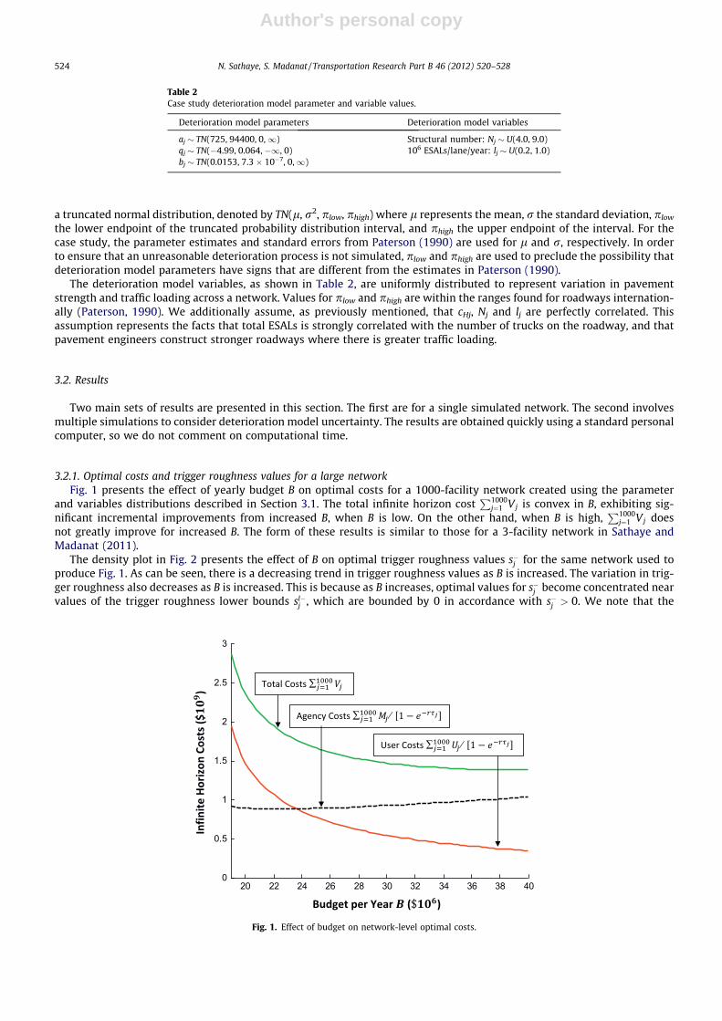
3.2.1. Optimal costs and trigger roughness values for a large networkFig. 1 presents the effect of yearly budget B on optimal costs for a 1000-facility network created using the parameter

and variables distributions described in Section 3.1. The total infinite horizon costP1000

j¼1 Vj is convex in B, exhibiting sig-nificant incremental improvements from increased B, when B is low. On the other hand, when B is high,

P1000j¼1 Vj does

not greatly improve for increased B. The form of these results is similar to those for a 3-facility network in Sathaye andMadanat (2011).

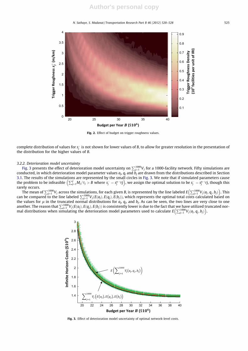
The density plot in Fig. 2 presents the effect of B on optimal trigger roughness values s�j for the same network used toproduce Fig. 1. As can be seen, there is a decreasing trend in trigger roughness values as B is increased. The variation in trig-ger roughness also decreases as B is increased. This is because as B increases, optimal values for s�j become concentrated nearvalues of the trigger roughness lower bounds sl�

j , which are bounded by 0 in accordance with s�j > 0. We note that the

Table 2Case study deterioration model parameter and variable values.

Deterioration model parameters Deterioration model variables

aj � TN(725, 94400, 0,1) Structural number: Nj � U(4.0, 9.0)qj � TN(�4.99, 0.064, �1, 0) 106 ESALs/lane/year: lj � U(0.2, 1.0)bj � TN(0.0153, 7.3 � 10�7, 0,1)

20 22 24 26 28 30 32 34 36 38 400

0.5

1

1.5

2

2.5

3

∑

∑ ⁄

∑ ⁄

Fig. 1. Effect of budget on network-level optimal costs.

524 N. Sathaye, S. Madanat / Transportation Research Part B 46 (2012) 520–528

Author's personal copy

complete distribution of values for s�j is not shown for lower values of B, to allow for greater resolution in the presentation ofthe distribution for the higher values of B.

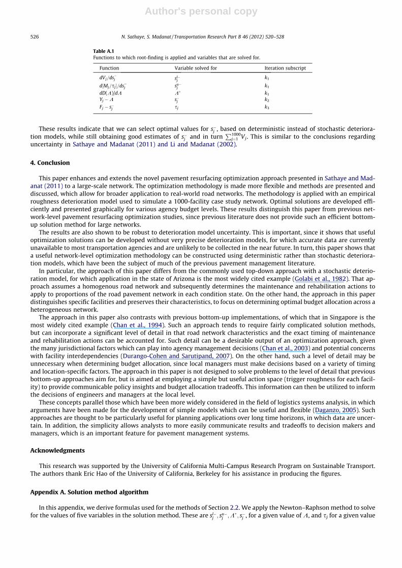
3.2.2. Deterioration model uncertaintyFig. 3 presents the effect of deterioration model uncertainty on

P1000j¼1 Vj for a 1000-facility network. Fifty simulations are

conducted, in which deterioration model parameter values aj, qj and bj are drawn from the distributions described in Section3.1. The results of the simulations are represented by the small circles in Fig. 3. We note that if simulated parameters causethe problem to be infeasible

PJj¼1Mj=sj > B where s�j ¼ su�

j 8j� �

, we assign the optimal solution to be s�j ¼ su�j 8j, though this

rarely occurs.The mean of

P1000j¼1 Vj across the simulations, for each given B, is represented by the line labeled E

P1000j¼1 Vjðaj; qj; bjÞ

� �. This

can be compared to the line labeledP1000

j¼1 VjðEðajÞ; EðqjÞ; EðbjÞÞ, which represents the optimal total costs calculated based onthe values for l in the truncated normal distributions for aj, qj, and bj. As can be seen, the two lines are very close to oneanother. The reason that

P1000j¼1 VjðEðajÞ; EðqjÞ; EðbjÞÞ is consistently lower is due to the fact that we have utilized truncated nor-

mal distributions when simulating the deterioration model parameters used to calculate EP1000

j¼1 Vjðaj; qj; bjÞ� �

.

20 25 30 35 400

0.5

1

1.5

2

2.5

3

3.5

4

0.1

0.2

0.3

0.4

0.5

0.6

0.7

0.8

0.9

Fig. 2. Effect of budget on trigger roughness values.

20 22 24 26 28 30 32 34 36 38 40

1.4

1.6

1.8

2

2.2

2.4

2.6

2.8

3

Fig. 3. Effect of deterioration model uncertainty of optimal network-level costs.

N. Sathaye, S. Madanat / Transportation Research Part B 46 (2012) 520–528 525

Author's personal copy

These results indicate that we can select optimal values for s�j , based on deterministic instead of stochastic deteriora-tion models, while still obtaining good estimates of s�j and in turn

P1000j¼1 Vj. This is similar to the conclusions regarding

uncertainty in Sathaye and Madanat (2011) and Li and Madanat (2002).

4. Conclusion

This paper enhances and extends the novel pavement resurfacing optimization approach presented in Sathaye and Mad-anat (2011) to a large-scale network. The optimization methodology is made more flexible and methods are presented anddiscussed, which allow for broader application to real-world road networks. The methodology is applied with an empiricalroughness deterioration model used to simulate a 1000-facility case study network. Optimal solutions are developed effi-ciently and presented graphically for various agency budget levels. These results distinguish this paper from previous net-work-level pavement resurfacing optimization studies, since previous literature does not provide such an efficient bottom-up solution method for large networks.

The results are also shown to be robust to deterioration model uncertainty. This is important, since it shows that usefuloptimization solutions can be developed without very precise deterioration models, for which accurate data are currentlyunavailable to most transportation agencies and are unlikely to be collected in the near future. In turn, this paper shows thata useful network-level optimization methodology can be constructed using deterministic rather than stochastic deteriora-tion models, which have been the subject of much of the previous pavement management literature.

In particular, the approach of this paper differs from the commonly used top-down approach with a stochastic deterio-ration model, for which application in the state of Arizona is the most widely cited example (Golabi et al., 1982). That ap-proach assumes a homogenous road network and subsequently determines the maintenance and rehabilitation actions toapply to proportions of the road pavement network in each condition state. On the other hand, the approach in this paperdistinguishes specific facilities and preserves their characteristics, to focus on determining optimal budget allocation across aheterogeneous network.

The approach in this paper also contrasts with previous bottom-up implementations, of which that in Singapore is themost widely cited example (Chan et al., 1994). Such an approach tends to require fairly complicated solution methods,but can incorporate a significant level of detail in that road network characteristics and the exact timing of maintenanceand rehabilitation actions can be accounted for. Such detail can be a desirable output of an optimization approach, giventhe many jurisdictional factors which can play into agency management decisions (Chan et al., 2003) and potential concernswith facility interdependencies (Durango-Cohen and Sarutipand, 2007). On the other hand, such a level of detail may beunnecessary when determining budget allocation, since local managers must make decisions based on a variety of timingand location-specific factors. The approach in this paper is not designed to solve problems to the level of detail that previousbottom-up approaches aim for, but is aimed at employing a simple but useful action space (trigger roughness for each facil-ity) to provide communicable policy insights and budget allocation tradeoffs. This information can then be utilized to informthe decisions of engineers and managers at the local level.

These concepts parallel those which have been more widely considered in the field of logistics systems analysis, in whicharguments have been made for the development of simple models which can be useful and flexible (Daganzo, 2005). Suchapproaches are thought to be particularly useful for planning applications over long time horizons, in which data are uncer-tain. In addition, the simplicity allows analysts to more easily communicate results and tradeoffs to decision makers andmanagers, which is an important feature for pavement management systems.

Acknowledgments

This research was supported by the University of California Multi-Campus Research Program on Sustainable Transport.The authors thank Eric Hao of the University of California, Berkeley for his assistance in producing the figures.

Appendix A. Solution method algorithm

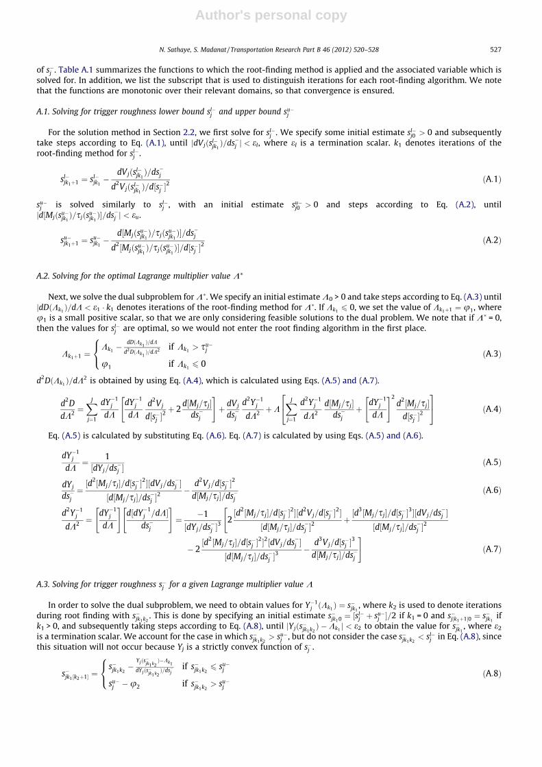
In this appendix, we derive formulas used for the methods of Section 2.2. We apply the Newton–Raphson method to solvefor the values of five variables in the solution method. These are sl�

j ; su�j ;K�; s�j , for a given value of K, and sj for a given value

Table A.1Functions to which root-finding is applied and variables that are solved for.

Function Variable solved for Iteration subscript

dVj=ds�j sl�j

k1

d½Mj=sj�=ds�j su�j k1

dD(K)/dK K� k1

Yj �K s�j k2

Fj � s�j sj k3

526 N. Sathaye, S. Madanat / Transportation Research Part B 46 (2012) 520–528

Author's personal copy

of s�j . Table A.1 summarizes the functions to which the root-finding method is applied and the associated variable which issolved for. In addition, we list the subscript that is used to distinguish iterations for each root-finding algorithm. We notethat the functions are monotonic over their relevant domains, so that convergence is ensured.

A.1. Solving for trigger roughness lower bound sl�j and upper bound su�

j

For the solution method in Section 2.2, we first solve for sl�j . We specify some initial estimate sl�

j0 > 0 and subsequentlytake steps according to Eq. (A.1), until jdVjðsl�

jk1Þ=ds�j j < el, where el is a termination scalar. k1 denotes iterations of the

root-finding method for sl�j .

sl�jk1þ1 ¼ sl�

jk1�

dVjðsl�jk1Þ=ds�j

d2Vjðsl�jk1Þ=d½s�j �

2ðA:1Þ

su�j is solved similarly to sl�

j , with an initial estimate su�j0 > 0 and steps according to Eq. (A.2), until

jd½Mjðsu�jk1Þ=sjðsu�

jk1Þ�=ds�j j < eu.

su�jk1þ1 ¼ su�

jk1�

d½Mjðsu�jk1Þ=sjðsu�

jk1Þ�=ds�j

d2½Mjðsu�jk1Þ=sjðsu�

jk1Þ�=d½s�j �

2ðA:2Þ

A.2. Solving for the optimal Lagrange multiplier value K⁄

Next, we solve the dual subproblem for K�. We specify an initial estimate K0 > 0 and take steps according to Eq. (A.3) untiljdDðKk1 Þ=dK < e1 � k1 denotes iterations of the root-finding method for K�. If Kk1 6 0, we set the value of Kk1þ1 ¼ u1, whereu1 is a small positive scalar, so that we are only considering feasible solutions to the dual problem. We note that if K� = 0,then the values for sl�

j are optimal, so we would not enter the root finding algorithm in the first place.

Kk1þ1 ¼Kk1� dDðKk1

Þ=dK

d2DðKk1Þ=dK2 if Kk1

> su�j

u1 if Kk16 0

8<: ðA:3Þ

d2DðKk1 Þ=dK2 is obtained by using Eq. (A.4), which is calculated using Eqs. (A.5) and (A.7).

d2D

dK2 ¼XJ

j¼1

dY�1j

dK

dY�1j

dKd2Vj

d½s�j �2 þ 2

d½Mj=sj�ds�j

" #þ dVj

ds�j

d2Y�1j

dK2 þKXJ

j¼1

d2Y�1j

dK2

d½Mj=sj�ds�j

þdY�1

j

dK

" #2d2½Mj=sj�

d½s�j �2

24

35 ðA:4Þ

Eq. (A.5) is calculated by substituting Eq. (A.6). Eq. (A.7) is calculated by using Eqs. (A.5) and (A.6).

dY�1j

dK¼ 1½dYj=ds�j �

ðA:5Þ

dYj

ds�j¼½d2½Mj=sj�=d½s�j �

2�½dVj=ds�j �½d½Mj=sj�=ds�j �

2 �d2Vj=d½s�j �

2

d½Mj=sj�=ds�jðA:6Þ

d2Y�1j

dK2 ¼dY�1

j

dK

" #d½dY�1

j =dK�ds�j

" #¼ �1

½dYj=ds�j �3 2½d2½Mj=sj�=d½s�j �

2�½d2Vj=d½s�j �2�

½d½Mj=sj�=ds�j �2 þ

½d3½Mj=sj�=d½s�j �3�½dVj=ds�j �

½d½Mj=sj�=ds�j �2

"

� 2½d2½Mj=sj�=d½s�j �

2�2½dVj=ds�j �½d½Mj=sj�=ds�j �

3 �d3Vj=d½s�j �

3

d½Mj=sj�=ds�j

#ðA:7Þ

A.3. Solving for trigger roughness s�j for a given Lagrange multiplier value K

In order to solve the dual subproblem, we need to obtain values for Y�1j ðKk1 Þ ¼ s�jk1

, where k2 is used to denote iterationsduring root finding with s�jk1k2

. This is done by specifying an initial estimate s�jk10 ¼ ½sl�j þ su�

j �=2 if k1 = 0 and s�j½k1þ1�0 ¼ s�jk1if

k1 > 0, and subsequently taking steps according to Eq. (A.8), until jYjðs�jk1k2Þ �Kk1 j < e2 to obtain the value for s�jk1

, where e2

is a termination scalar. We account for the case in which s�jk1k2> su�

j , but do not consider the case s�jk1k2< sl�

j in Eq. (A.8), sincethis situation will not occur because Yj is a strictly convex function of s�j .

s�jk1 ½k2þ1� ¼s�jk1k2

�Yjðs�jk1k2

Þ�Kk1

dYjðs�jk1k2Þ=ds�j

if s�jk1k26 su�

j

su�j �u2 if s�jk1k2

> su�j

8<: ðA:8Þ

N. Sathaye, S. Madanat / Transportation Research Part B 46 (2012) 520–528 527

Author's personal copy

A.4. Solving for overlay interval sj for a given trigger roughness s�j

In order to solve for sl�jk1; su�

jk1; s�jk1k2

, and indirectly for Kk1 we require a values for sj. To make the discussion more concise,we will discuss the root finding method only with sjk1k2k3 , which satisfies Fjðsjk1k2k3 ; s

þjk1k2Þ ¼ s�jk1k2

; however the same general

method is applied when solving for sl�jk1

and su�jk1

. k3 is used to denote iterations during root finding for sjk1k2 . We note that

sþjk1k2¼ s�jk1k2

½1� gj� is held constant while solving for sjk1k2 , so Fj is simplified to being a monotonic function of sj 2 ½sl�j ; su�

j �.We specify an initial estimate sjk1k20 ¼ ½sl�

j þ su�j �=2 if k2 = 0 and sjk1 ½k2þ1�0 ¼ sjk1k2 if k2 > 0, and subsequently take steps

according to Eq. (A.9), until jFjðsjk1k2k3 ; sþjk1k2Þ � s�jk1k2

j < e3 to obtain the value for sjk1k2 , where e3 is a termination scalar.

Fjðsj; sþj Þ is a strictly convex function of sj. Therefore s�jk1k2k3< sl�

j does not occur and we do not consider this case in Eq. (A.9).

sjk1k2 ½k3þ1� ¼sjk1k2k3

�Fjðsjk1k2k3

;sþjk1k2

Þ�s�jk1k2

@Fjðsjk1k2k3;sþ

jk1k2Þ=@t if sjk1k2k3

6 su�j

su�j if sjk1k2k3 > su�

j

8<: ðA:9Þ

References

American Society of Civil Engineers, 2009. Report Card for America’s Infrastructure.Bazaraa, M., Sherali, H., Shetty, C., 2006. Nonlinear Programming: Theory and Applications. Wiley-Interscience.Chan, W., Fwa, T., Tan, C., 1994. Road-maintenance planning using genetic algorithms. I: Formulation. Journal of Transportation Engineering 120 (5), 693–

709.Chan, W., Fwa, T., Tan, J.Y., 2003. Optimal fund-allocation analysis for multidistrict highway agencies. Journal of Infrastructure Systems 9 (4), 167–175.Chootinan, P., Chen, A., Horrocks, M., Bolling, D., 2006. A multi-year pavement maintenance program using a stochastic simulation-based genetic algorithm

approach. Transportation Research Part A 40 (9), 725–743.Daganzo, C., 2005. Logistics Systems Analysis, fourth ed. Springer.Durango-Cohen, P., Sarutipand, P., 2007. Capturing interdependencies and heterogeneity in the management of multifacility transportation infrastructure

systems. Journal of Infrastructure Systems 13 (2), 115–123.Fernandez, E., Friesz, T., 1981. Influence of demand-quality interrelationships on optimal policies for stage construction of transportation facilities.

Transportation Science 15 (1), 16–31.Ferreira, A., de Picado-Santos, L., Wu, Z., Flintsch, G., 2011. Selection of pavement performance models for use in the Portuguese PMS. International Journal

of Pavement Engineering 12 (1), 87–97.Friesz, T., Fernandez, E., 1979. A model of optimal transport maintenance with demand responsiveness. Transportation Research Part B 13 (4), 317–339.Golabi, K., Kulkarni, R., Way, G., 1982. A statewide pavement management system. Interfaces 12 (6), 5–21.Ibaraki, T., Katoh, N., 1988. Resource Allocation Problems: Algorithmic Approaches. MIT Press.Kuhn, K., Madanat, S., 2005. Model uncertainty and the management of a system of infrastructure facilities. Transportation Research Part C 13 (5-6), 391–

404.Li, Y., Madanat, S., 2002. A steady-state solution for the optimal pavement resurfacing problem. Transportation Research Part A 36 (6), 525–535.Lidicker, J., Sathaye, N., Madanat, S., Horvath, A. (forthcoming). Pavement resurfacing policy for minimization of life-cycle costs and greenhouse gas

emissions. Journal of Infrastructure Systems.Markow, M., Balta, W., 1985. Optimal rehabilitation frequencies for highway pavements. Transportation Research Record 1035, 31–43.McPherson, K., Bennett, C., 2005. Success Factors for Road Management Systems. East Asia Pacific Transport Unit, The World Bank.Melachrinoudis, E., Kozanidis, G., 2002. A mixed integer knapsack model for allocating funds to highway safety improvements. Transportation Research Part

A 36 (9), 789–803.Ouyang, Y., Madanat, S., 2004. Optimal scheduling of rehabilitation activities for multiple pavement facilities: exact and approximate solutions.

Transportation Research Part A 38 (5), 347–365.Ouyang, Y., Madanat, S., 2006. An analytical solution for the finite-horizon pavement resurfacing planning problem. Transportation Research Part B 40 (9),

767–778.Paterson, W.D.O., 1990. Quantifying the effectiveness of pavement maintenance and rehabilitation. In: Proceedings at the 6th REAAA Conference, Kuala

Lumpur, Malaysia.Patriksson, M., 2008. A survey on the continuous nonlinear resource allocation problem. European Journal of Operational Research 185 (1), 1–46.Robelin, C.-A., Madanat, S., 2008. Reliability-based system-level optimization of bridge maintenance and replacement decisions. Transportation Science 42

(4), 508–513.Santero, N., Horvath, A., 2009. Global warming potential of pavements. Environmental Research Letters 4 (3).Sathaye, N., Madanat, S., 2011. A bottom-up solution for the multi-facility optimal pavement resurfacing problem. Transportation Research Part B 45 (7),

1004–1017.Sathaye, N., Horvath, A., Madanat, S., 2010. Unintended impacts of increased truck loads on pavement supply-chain emissions. Transportation Research Part

A 44 (1), 1–15.Yeo, H., Yoon, Y., Madanat, S., forthcoming. Algorithms for Bottom-Up Maintenance Optimization for Heterogeneous Infrastructure Systems. Structure and

Infrastructure Engineering.

528 N. Sathaye, S. Madanat / Transportation Research Part B 46 (2012) 520–528