A Bonus-Malus Framework for Cyber Risk Insurance and ...

A Bonus-Malus Framework for Cyber Risk Insurance and

Optimal Cybersecurity Provisioning

Qikun Xiang1, Ariel Neufeld1, Gareth W. Peters2, Ido Nevat3, and Anwitaman Datta4

1Division of Mathematical Sciences, Nanyang Technological University, Singapore

2Department of Actuarial Mathematics and Statistics, Heriot-Watt University, Edinburgh, UK

3TUMCREATE, Singapore

4School of Computer Science and Engineering, Nanyang Technological University, Singapore

Abstract

The cyber risk insurance market is at a nascent stage of its development, even as the magnitude

of cyber losses is significant and the rate of cyber risk events is increasing. Existing cyber risk

insurance products as well as academic studies have been focusing on classifying cyber risk events

and developing models of these events, but little attention has been paid to proposing insurance

risk transfer strategies that incentivize mitigation of cyber loss through adjusting the premium

of the risk transfer product. To address this important gap, we develop a Bonus-Malus model

for cyber risk insurance. Specifically, we propose a mathematical model of cyber risk insurance

and cybersecurity provisioning supported with an efficient numerical algorithm based on dynamic

programming. Through a numerical experiment, we demonstrate how a properly designed cyber risk

insurance contract with a Bonus-Malus system can resolve the issue of moral hazard and benefit the

insurer.

Keywords—Cyber risk insurance, Cybersecurity, Bonus-Malus, Stochastic optimal control, Dy-

namic programming

1 Introduction

1.1 The Ever-Increasing Threat of Cyber Crimes

Over the years, the frequency and severity of cyber attacks have increased significantly globally, and will

continue to increase in the future. Recently, Cybersecurity Ventures estimated the cost of cyber crimes

to rise to 10.5 trillion USD annually by 2025 (Morgan, 2020), up from a world economic forum estimate

of 3 trillion USD for 2015. The world economic forum’s annual global risk report (Franco, 2020) regularly

puts cyber attacks and theft of data in its “Top 5 global risks in terms of likelihood”.

Cyber crime is being perpetrated on a massive scale, over a range of different actors in society, hitting

individuals in their personal environment as well as organisations. Cyber crime is also a risk type that

1

arX

iv:2

102.

0556

8v1

[m

ath.

OC

] 1

0 Fe

b 20

21

affects a large array of different organisations worldwide, e.g. government agencies, universities, financial

sectors, private corporations, and generally across all industries, including important infrastructure units

that play a key role in population security and safety, such as emergency services and health care. Such

attacks have caused breaches and significant damages to those organizations, which are vulnerable to

intrusion, and often adversely affect downstream users of the compromised services and organizations.

The damages incurred can include losses attributed to outcomes such as business interruption, loss of

data, reduced reputation and trust of the organisation, legal liabilities, intellectual property theft, and

potential for loss of life. These damages result in various degrees of financial loss, including devastating

losses as well as ongoing high frequency losses. Cyber attacks can be initiated by both malicious actors

within institutions and also external to institutions such as cyber criminals, rogue nation states, hackers,

cyber terrorists, and others with malicious intent causing significant negative impact and cost.

Cyber attacks come in a variety of forms, ranging from from denial-of-service (DoS) attacks (Gupta

and Badve, 2017), malware (Tailor and Patel, 2017), ransomware (Tailor and Patel, 2017), blackmail

(Rid and McBurney, 2012), extortion (Young and Yung, 1996), and more (Craigen, Diakun-Thibault,

and Purse, 2014; Husak, Komarkova, Bou-Harb, and Celeda, 2019). Many forms of cyber attacks can

weaponize third party infrastructure and are not bounded by geographical distance, and hence do not

require specialised equipment to devise and initiate. The seriousness of Cyber attacks has been reflected

in the U.S. President’s executive order on Strengthening the Cyber security of Federal Networks and

Critical Infrastructure, which calls for a cybersecurity framework that can “support the cybersecurity

risk management efforts of the owners and operators of the Nation’s critical infrastructure”. Cyber

risk from a financial and insurance perspective has also been developed under international banking

and insurance regulations, where the Basel III banking accords cover cyber risk as a key component of

Operational Risk captial modeling and adequacy, and the Solvency II insurance regulations discuss the

significance of an emerging cyber insurance threat that affects both insurers as well as reinsurers. For

example, see an overview of cyber risk from a financial and insurance perspective in Peters, Shevchenko,

and Cohen (2018b).

Financial and governmental regulatory bodies largely classify cyber events according to the following

categories:

1. System malfunctions/issue – own system or network is malfunctioning or creating damage to third-

party’s systems or supplier’s system not functioning, impacting own digital operations;

2. Data confidentiality breach – data stored in own system (managed on premise or hosted/managed

by third party) has been stolen and exposed;

3. Data integrity/availability – data stored in own system (managed on premise or hosted/managed

by third party) have been corrupted or deleted;

4. Malicious activity – misuse of a digital system to inflict harm (such as cyber bullying over social

platforms or phishing attempts to then delete data) or to illicitly gain profit (such as cyber fraud).

As an example, consider the Federal Information Security Management Act of 2002 (FISMA), which

2

states their working definition of cyber crime and information security in such a manner as to link the

identified operational cybersecurity risks to specific examples of consequences impacting confidential-

ity, integrity, and availability: “Information Security: means protecting information and information

systems from unauthorized access, use, disclosure, disruption, modification, or destruction in order to

provide: integrity, which means guarding against improper information modification or destruction, and

includes ensuring information non repudiation and authenticity; confidentiality, which means preserving

authorized restrictions on access and disclosure, including means for protecting personal privacy and

proprietary information; and availability, which means ensuring timely and reliable access to and use of

information.”

1.2 The Need for Better Models for Cyber Risk Insurance

Although many different security solutions have been developed and implemented in order to detect and

prevent cyber attacks, achieving a complete security protection is not feasible (Lu, Niyato, Privault,

Jiang, and Wang, 2018b). To address this problem, there is an increasing demand to develop the market

for cyber risk insurance and to understand the structuring of insurance products that will facilitate risk

transfer strategies in the context of cyber risk and financial risk, see discussions in Peters et al. (2018b);

Peters, Shevchenko, and Cohen (2018a); Marotta, Martinelli, Nanni, Orlando, and Yautsiukhin (2017);

Bohme and Schwartz (2010) and the references therein. The confluence of increasing sophistication and

frequency of cyber attacks on IT infrastructure, the increasing collections of sensitive data in private

enterprises and government agencies coupled with the onset of emerging regulatory frameworks, such as

Basel II/III and the insurance regulation of Solvency II which contain core requirements related to cyber

risk mitigation and modeling have prompted the study of questions pertaining how best to develop a

cyber risk insurance market place.

As one can see from surveys such as Marotta et al. (2017) and Shetty, Schwartz, Felegyhazi, and

Walrand (2010) the scope of such a market place is still very much in its infancy. This has occurred in

the insurance space despite the fact that banks and financial institutions rank cyber event losses in their

top three loss events systematically when reporting Operational Risk loss events under Basel II/III to

national regulators. The reason that the cyber insurance market has yet to emerge with standardised

products has largely arisen due to differences in opinion as how best to mitigate and reserve against

these loss events. From the IT perspectives, it is common to take a technology perspective to attempt

to mitigate such events in contrast to insurance or capital reserving, see discussions in Bandyopadhyay,

Mookerjee, and Rao (2009). From a financial risk perspective, risk practitioners see cyber risk from

the Operational Risk Basel II/III accord perspective and attempt to avoid insurance mitigation, instead

opting for Tier I capital reserving, as the capital reduction from Operational Risk insurance is capped

under Basel regulations with a haircut of 20%, see discussions in Peters, Byrnes, and Shevchenko (2011),

disincentivizing them to purchase insurance products that have excessive premiums. From the insurance

industry’s perspective, there is a lack of market standardisation on insurance contract specifications

that would avoid excessive premiums being required to be charged when bespoke insurance products are

designed.

3

These three perspectives are beginning to change and we believe it is now a suitable time to revisit

the perennial question of how best to set up an insurance market place for cyber risk events. From

a technological perspective, cybersecurity is achieved by applying multiple controls which span across

being preventive, detective and corrective, and thus realizing defense in depth. For instance, for defense

against a distributed denial-of-service (DDoS) attack which would violate the availability property of a

service, an organization may opt to use network traffic filtering as well as a content distribution network,

and use multiple servers to balance the network load. The life-cycle of a data breach event often involves

the initial intrusion event, subsequent escalation of privileges till the exfiltration of data. The victim

thus has a window of opportunity from the moment of intrusion to the eventual breach of the data, to

detect and prevent it. An organization may also invest in storing the data encrypted. As such, there

are various controls for ensuring confidentiality property in this instance, but each control adds to the

upfront costs of risk prevention or reduction. An organization needs to determine the quantum of its

security (risk prevention) budget and distribute this across these controls. We argue that this budget for

risk reduction needs to and can be determined in tandem with risk transfer decisions. In particular, we

want to explore a model where an organization enjoys a reduction in the cost of risk transfer as a result

of its upfront expenses in risk reductions; and like-wise an insurer benefits from a pricing model which

encourages good security posture among its customers.

1.3 The Proposed Cyber Risk Framework

We propose in this paper a perspective that combines classical market place structuring via a Bonus-

Malus framework that provides IT-specific incentive mechanisms that act to encourage sound IT gover-

nance and technology developments, whilst also allowing insurers to encourage risk reduction in their risk

pools to provide competitive insurance premium pricing. We introduce for the first time a cyber risk-

based Bonus-Malus framework and then demonstrate how to develop loss models and decision making

models under uncertainty in this framework from both individual and insurance providers’ perspectives.

1.4 Related Work

Recently, many studies analyzed the cyber risk insurance from a technology perspective. Security frame-

works involving cyber risk insurance have been developed for specific IT systems, including computer

networks (Fahrenwaldt, Weber, and Weske, 2018; Xu and Hua, 2019), heterogeneous wireless network

(Lu, Niyato, Jiang, Wang, and Poor, 2018a), wireless cellular network (Lu et al., 2018b), plug-in electric

vehicles (Hoang, Wang, Niyato, and Hossain, 2017), cloud computing (Chase, Niyato, Wang, Chaisiri,

and Ko, 2019), and fog computing (Feng, Xiong, Niyato, Wang, and Leshem, 2018).

Some studies considered the interplay between self-mitigation measures (i.e. risk reduction) and cyber

risk insurance, e.g. Pal and Golubchik (2010); Pal, Golubchik, Psounis, and Hui (2014, 2019); Khalili,

Naghizadeh, and Liu (2018); Dou, Tang, Wu, Qi, Xu, Zhang, and Hu (2020). These studies investigated

two important challenges in cyber risk insurance: risk interdependence and moral hazard. They found

that in order to incentivize the insured to invest in self-mitigation measures, some form of contract

4

discrimination, i.e. adjusting the insurance premium based on the insured’s security investment, is nec-

essary. Yang and Lui (2014); Schwartz and Sastry (2014); Zhang, Zhu, and Hayel (2017) investigated

these challenges in a networked environment, where cyber attacks can spread between neighboring nodes,

further complicating these challenges.

There are also studies which took the insured’s perspective and analyzed the security provisioning

process using dynamic models. Chase et al. (2019) developed a framework based on stochastic opti-

mization to jointly provision cyber risk insurance and cloud-based security services across multiple time

periods in cloud computing applications. Zhang and Zhu (2018) modeled the decisions on self-protections

of the insured by a Markov decision process and investigated the problem of insurance contract design.

A critical drawback of many of the existing studies is that they neglected the highly uncertain nature

of losses incurred by cyber incidents. These studies relied on over-simplified assumptions, e.g. by modeling

cyber loss as: a fixed amount (Pal and Golubchik, 2010; Pal et al., 2014; Yang and Lui, 2014; Hoang

et al., 2017; Feng et al., 2018; Dou et al., 2020), random with finite support (Chase et al., 2019; Zhang

and Zhu, 2018; Lu et al., 2018b), or random with a simple parametric distribution (Zhang et al., 2017;

Khalili et al., 2018). These assumptions limit the practicality of these studies, and their results remain

conceptual and non-applicable to realistic insurance loss modeling under a classical Loss Distributional

Approach (LDA) framework. Moreover, many of these studies do not take into account the interplay

between the upfront costs of prevention, the consequent reduced risks, and the possibility to exploit this

interplay to design practical cyber risk insurance products.

A review of cyber insurance product prospectus by major insurers, such as AIG’s CyberEgde1, Allianz

Cyber Protect2, and Chubb’s Cyber Enterprise Risk Management (Cyber ERM)3 indicates that the

insurance products in the market have yet to explicitly factor in the benefits of up-front protection, or

to incentivize and offset those costs against that of risk transfer. We introduce the Bonus-Malus system

which is frequently used in vehicle insurance products to address this gap in cyber risk product design.

1.5 Contributions

Our main contributions are as follows:

1. We introduce the Bonus-Malus system to cyber risk insurance as a mechanism to provide incentive

for the insured to adopt self-mitigation measures against cyber risk.

2. We develop a mathematical model of cyber losses and cyber risk insurance, and subsequently

analyze the optimal cybersecurity provisioning process of the insured under the stochastic optimal

control framework.

3. We develop an efficient algorithm based on dynamic programming to accurately solve the stochastic

optimal control problem, under the assumption that the loss severity follows a truncated version

1https://www.aig.com/business/insurance/cyber-insurance/, accessed on 2020-12-102https://www.agcs.allianz.com/solutions/financial-lines-insurance/cyber-insurance.html, accessed on 2020-

12-103https://www.chubb.com/us-en/business-insurance/cyber-enterprise-risk-management-cyber-erm.html,

accessed on 2020-12-10

5

of the g-and-h distribution. We also formally prove the correctness of the proposed algorithm.

4. We demonstrate through a numerical experiment that a properly designed cyber risk insurance

contract with a Bonus-Malus system can resolve the issue of moral hazard, and can provide benefits

for the insurer.

1.6 Organization of the Paper

The rest of the paper is organized as follows. In Section 2, we introduce the mathematical model of

cyber losses and cyber risk insurance with a Bonus-Malus system. In Section 3, we present the optimal

cybersecurity provisioning process and the dynamic programming algorithm. In Section 4, we introduce

the g-and-h distribution and use it as the model for loss severity. We present results from the numerical

experiment in Section 5. Finally, Section 6 concludes the paper.

2 Cyber Risk Insurance Policy and Bonus-Malus System

Let us first present an overview of our cyber risk insurance model, which begins with a specification of

the frequency and severity model under consideration in the Loss Distributional Approach (LDA) that

defines the financial loss process that results from cyber risk events. We consider T ∈ N consecutive

years, and we assume that throughout each year t, the insured may suffer a random number (Nt ∈ N)

of cyber loss events arising from cyber attack events. These loss amounts are denoted by X(t)1 , . . . , X

(t)Nt

.

The cumulative annual cyber loss in year t is therefore∑Ntk=1X

(t)k . Such a loss model is referred to as the

Loss Distributional Approach (LDA) in the study of Operational Risk. The insured has several choices

to attempt to mitigate these cyber events and reduce the risk, including enhancing the security and

resilience of their IT infrastructure and reserving Tier I capital to cover the incurred losses. In regards to

the internal IT infrastructure, it will be assumed that the insured has the option to adopt a self-mitigation

measure that can reduce the severity of cyber incidents up to a fixed amount of loss corresponding to

the effect of the self-mitigation measure. In addition, the insured can choose to purchase a cyber risk

insurance policy which gives the insured the right to claim the cumulative cyber loss incurred, up to

a maximum cap imposed by the insurance contract, in an agreed interval of time (typically annually),

minus a deductible.

2.1 Cyber Loss Model

Let us defineW :=⋃n∈Z+

n×Rn+ to be the space representing all possible combinations of realizations

of the number of events per year (frequency) and individual losses per event (severities). Let B(W) :=

σ(⋃n∈Z+

(n,B) : B ∈ B(Rn+)) be a σ-algebra on W, where B(Rn+) denotes the Borel subsets of Rn+.

Let us consider the space Ω := (W)T =W × · · · ×W︸ ︷︷ ︸T times

. For each ω = (w1, . . . , wT ) = ((n1, x(1)1 , . . . , x

(1)n1 ),

. . . , (nT , x(T )1 , . . . , x

(T )nT )) ∈ Ω, we define Wt(ω) := wt and Nt(ω) := nt for t = 1, . . . , T . Let P1 be a

probability measure on (W,B(W)), where the subscript “1” indicates that it is a probability measure

6

for the cyber incidents occuring in a single year. Let P := P1 ⊗ · · · ⊗ P1︸ ︷︷ ︸T times

, and let (Ft)t=0:T be a filtration

on Ω, defined by F0 := ∅,Ω, Ft := σ((Ws)s=1:t). Then, (Ω,FT ,P, (Ft)t=0:T ) is a filtered probability

space. Under these definitions, W1, . . . ,WT are independently and identically distributed (i.i.d.) random

variables. Let ψN (s) := E[sN1 ] denote the probability generating function (pgf) of the loss frequency

distribution. We assume that for t = 1, . . . , T ,

P[ω = ((n1, x(1)1 , . . . , x(1)

n1), . . . , (nT , x

(T )1 , . . . , x(T )

nT )) : nt = n, x(t)k ≤ zk, k = 1, . . . , n]

=P[Nt = n]

n∏k=1

FX(zk),(1)

where FX(·) is a distribution function corresponding to the severity distribution. This implies that

given the loss frequency of a year, the individual loss amounts in that year are i.i.d. We assume

that the severity distribution has finite expectation, i.e.∫R |x|dFX < ∞. For convenience, we write

Wt =(Nt, X

(t)1 , . . . , X

(t)Nt

). We use W to refer to a random variable that has the same distribution

as W1, . . . ,WT . Similarly, we use N to refer to a random variable that has the same distribution as

N1, . . . , NT , and we use X to refer to a random variable that has distribution function FX .

2.2 Self-Mitigation Measures

Let us assume that there exists D ∈ N different self-mitigation measures, and the insured makes the

decision to either adopt one of the self-mitigation measures or to not adopt any self-mitigation measure

at the beginning of each year. The self-mitigation measure d ∈ D := 0, 1, . . . , D requires an annual

investment of β(d) ∈ R+ per year, and decreases the severity of each cyber loss by up to γ(d) ∈ R+, that

is, the severity of a loss will be decreased from X to (X − γ(d))+4 with the adoption of the self-mitigation

measure d. We assume that β(0) = γ(0) = 0. Thus, if the insured decides to adopt the self-mitigation

measure d in a year, then the total loss suffered by the insured that year is given by

L(d,w) :=

n∑k=1

(xk − γ(d))+, (2)

when the corresponding loss frequency and severity that year is w = (n, x1, . . . , xn) ∈ W.

2.3 Cyber Risk Insurance Policy

Let us now consider a cyber risk insurance contract that lasts for T years. At the beginning of each year,

the insured decides whether to activate the contract. In the case that the contract has been activated

in a previous year, this corresponds to the insured deciding whether to continue the contract. If the

contract is activated, the insured pays a premium to the insurer at the start of the year, in exchange

for the insurance coverage throughout the year. If the insured decides to withdraw from the contract,

it no longer pays the premium and the contract is deactivated so that the insured receives no coverage.

We further assume that the insured pays the insurer an initial sign-on fee for fixed costs and contract

origination the first time a contract is initiated, in addition to the premium, and that this amount varies

4Throughout the paper, we use the following notations: (x)+ := maxx, 0, x∨ y := maxx, y and x∧ y := minx, y.

7

deterministically over time and will be denoted by δin(t) ≥ 0 in year t. This can be used to incentivize

the insured to activate the contract early. Furthermore, we also assume that the insured pays the insurer

a deterministic and time-dependent penalty, denoted by δout(t) ≥ 0, when it withdraws from the contract

in year t. Once withdrawn, the insured may re-activate the contract at a later year with a fixed penalty

δre ≥ 0.

Suppose that the cumulative cyber loss suffered by the insured in a year is L. At the end of the year,

the insured decides whether to make a claim to the insurer. Once the claim is processed, the insured

receives a payment of (L− ldtb)+∧ lmax from the insurer as compensation, that is, the insured covers the

loss up to the deductible ldtb ≥ 0, and the insurer covers all of the remaining loss up to the maximum

compensation lmax ≥ 0.

2.4 Bonus-Malus System

We now introduce the Bonus-Malus system to cyber risk insurance markets. Let us assume that there are

B Bonus-Malus levels in the contract, denoted by B := −B, . . . ,−1, 0, 1, . . . , B, where B+B+ 1 = B.

At t = 0, the insured starts in the initial Bonus-Malus level, denoted by b0 = 0. At the end of the t-th

year, given that the contract is still active, the insurer determines the Bonus-Malus level of the insured

based on its previous level bt−1, and the amount of insurance claims Ct that was given out to this insured

in the t-th year, that is, bt = BM(bt−1, Ct), where BM : B×R+ → B denotes the deterministic rules that

are transparent to the insured at the signing of the contract. We make the assumption that BM(b, C) is

non-decreasing in C for each b ∈ B. Even when the insured has withdrawn from the contract, we assume

that the Bonus-Malus level is still updated annually. Concretely, let us define I := no, on, off1, . . . , offT

as the set of all possible states of the cyber risk insurance contract. In I, “no” denotes that the contract

has not been signed yet, “on” denotes that the contract is continued, and “offy” denotes that the contract

is withdrawn and y ∈ Z+ represents the counter variable that is updated annually as long as the insured

does not re-activate the contract. Let BM0 : B × I → B × I be a deterministic transition function that

represents the update rules after the insured withdraws from the contract. At the end of the t-th year,

given that the contract is inactive, the insurer determines the Bonus-Malus level bt and the insurance

state it of the insured based on its Bonus-Malus level and the insurance state in the previous year, that

is, (bt, it) = BM0(bt−1, it−1). Since no such update is possible before the insured activates the contract,

it is required that BM0(b,no) = (b,no) for all b ∈ B.

With the addition of the Bonus-Malus system to the cyber risk insurance, we assume that the premium

depends on both time and the current Bonus-Malus level of the insured, and is given by pBM(b, t),

where pBM : B × 1, . . . , T → R+ is a deterministic function. The deductible and the maximum

compensation are also assumed to be dependent on both time and the Bonus-Malus level, and are given

by deterministic functions lBMdtb : B × 1, . . . , T → R+ and lBMmax : B × 1, . . . , T → R+. We define the

function λBM : B × 1, . . . , T × R+ → R+ by

λBM(b, t, l) := (l − lBMdtb (b, t))+ ∧ lBMmax(b, t) (3)

to simplify the notation when modeling the loss covered by the insurer.

8

3 Optimal Cybersecurity Provisioning and Stochastic Optimal

Control

3.1 Cybersecurity Provisioning Process

Now, having introduced the model for cyber losses and cyber risk insurance, we consider the problem of

optimal cybersecurity provisioning from the insured’s point of view.

It is assumed that the cybersecurity provisioning process takes place for T consecutive years (same

as the length of the cyber risk insurance), and each year consists of the three following stages:

1. Provision Stage. The insured decides: (i) the self-mitigation measure to adopt in this year,

denoted by dt ∈ D and (ii) whether to activate/withdraw/rejoin the cyber risk insurance contract,

denoted by ιt ∈ 0, 1.

2. Operation Stage. The random cyber risk events and the corresponding cyber losses suffered by

the insured in this year, denoted by Wt, is realized in this stage according to the model described

in Section 2.1 and Section 2.2.

3. Claim Stage. If the insurance contract is active, the insured decides whether or not to make a

claim, denoted by jt ∈ 0, 1. In the case where a claim is made, the insured receives a compensation

from the insurer corresponding to the cyber loss that year. Subsequently, the Bonus-Malus level

of the insured is updated.

Formally, let

Π :=π = (dt, ιt,jt)t=1:T : dt : Ω→ D, ιt : Ω→ 0, 1 are Ft−1-measurable,

jt : Ω→ 0, 1 is Ft-measurable, ιt = 0, jt = 1 = ∅, for t = 1, . . . , T (4)

denote the set of all possible decision policies. The conditions in the above definition are explained as

follows:

• The decisions dt, ιt are made before observing Wt, hence may depend on all available information

up to year t− 1;

• The decision jt is made after observing Wt, hence may depend on all available information up to

year t;

• The condition ιt = 0, jt = 1 = ∅ requires that the insured may only make a claim (i.e. jt = 1)

when the insurance is adopted (i.e. ιt = 1) in year t.

For t = 1, . . . , T , let ft : B × I × D × 0, 1 × 0, 1 ×W → B × I be the state transition function for

each year t, given by

ft(b, i, d, ι, j, w) :=

(BM(b, jλBM(b, t, L(d,w))), on

), if ι = 1,

BM0(b, i) if ι = 0.

(5)

9

For t = 1, . . . , T , let gt : B×I ×D×0, 1×0, 1×W → R+ be the cost function for each year t, given

by

gt(b, i, d, ι, j, w) :=β(d) + ιpBM(b, t) + δin(t)1i=no,ι=1 + δout(t)1i=on,ι=0

+ δre1i6=on,i6=no,ι=1 + L(d,w)− ιjλBM(b, t, L(d,w)),(6)

where β(d) is the investment of adopting the self-mitigation measure d, ιpBM(b) corresponds to the

cyber risk insurance premium, δin(t)1i=no,ι=1 + δout(t)1i=on,ι=0 + δre1i 6=on,i6=no,ι=1 corresponds to

the entrance/withdrawal costs, L(d,w) is the total cyber loss, and ιjλBM(b, t, L(d,w)) corresponds to

the compensation from the insurer.

Now, for any decision policy π = (dt, ιt, jt)t=1:T ∈ Π, let us define the (Ft)t=0:T -adapted controlled

stochastic process(bπt , i

πt

)t=0:T

as follows:

(bπ0 , iπ0 ) :=(0,no),

(bπt , iπt ) :=ft(b

πt−1, i

πt−1, dt, ιt, jt,Wt) for t = 1, . . . , T.

(7)

Then, gt(bπt−1, i

πt−1, dt, ιt, jt,Wt) corresponds to the cybersecurity cost in year t. For π ∈ Π, and t =

1, . . . , T , define V πt by

V πt := E[∑T

s=t+1 e−(s−t)rgs(b

πs−1, i

πs−1, ds, ιs, js,Ws)

∣∣∣Ft], (8)

where 0 < e−r ≤ 1 is the discount factor and V πT := 0.

We assume that in the cybersecurity provisioning process, the objective of the insured is to minimize

the expected value of the discounted total cybersecurity cost. This is formulated as the following finite

horizon stochastic optimal control problem:

V0 := infπ∈Π

V π0 = infπ∈Π

E[∑T

t=1 e−trgt(b

πt−1, i

πt−1, dt, ιt, jt,Wt)

]. (9)

3.2 Dynamic Programming Algorithm

The stochastic optimal control problem introduced in Section 3.1 can be solved efficiently via the dynamic

programming algorithm. The dynamic programming algorithm iteratively solves a sequence of one-

stage optimization problems and also constructs an optimal decision policy from the optimizers of these

problems. In the following, we define the values of these one-stage optimization problems, denoted by

(Vt)t=0:T , and their corresponding optimizers (dt, ιt, jt)t=1:T .

For t = T, T − 1, . . . , 0, let Vt : B × I → R+ be recursively defined as follows: for every b ∈ B, i ∈ I,

let

VT (b, i) :=0,

Vt−1(b, i) :=e−r mind∈D,ι∈0,1

E[

minj∈0,1

gt(b, i, d, ι, j,W ) + Vt

(ft(b, i, d, ι, j,W )

)].

(10)

For t = 1, . . . , T , let dt : B × I → D, ιt : B × I → 0, 1, and jt : B × I × W → 0, 1 be defined as

10

follows: for every b ∈ B, i ∈ I, let

(dt(b, i), ιt(b, i)

)∈ arg mind∈D,ι∈0,1

E[

minj∈0,1

gt(b, i, d, ι, j,W ) + Vt

(ft(b, i, d, ι, j,W )

)], (11)

jt(b, i, w) :=

1 if ιt(b, i) = 1,

[gt(b, i, dt(b, i), 1, 1, w) + Vt

(ft(b, i, dt(b, i), 1, 1, w)

)]<[gt(b, i, dt(b, i), 1, 0, w) + Vt

(ft(b, i, dt(b, i), 1, 0, w)

)],

0 otherwise.

(12)

The following theorem shows the construction of an optimal decision policy by dynamic programming.

Theorem 3.1. Let (Vt)t=0:T be defined as in (10), let the functions (dt, ιt, jt)t=1:T be defined as in (11)

and (12), and let π? = (d?t , ι?t , j

?t )t=1:T ∈ Π be recursively defined as follows:(

bπ?

0 , iπ?

0

):= (0,no),

for t =1, . . . , T, let:

d?t := dt(bπ?

t−1, iπ?

t−1

), ι?t := ιt

(bπ?

t−1, iπ?

t−1

), j?t := jt

(bπ?

t−1, iπ?

t−1,Wt

).

(13)

Then, the following holds:

V0(0,no) = V π?

0 = V0. (14)

Proof. See Appendix A.

As a consequence of Theorem 3.1, let us now introduce an algorithm based on the dynamic program-

ming principle to solve the stochastic optimal control problem (9), which is presented in Algorithm 1. In

addition to an optimal decision policy π?, Algorithm 1 also outputs the state transition probabilities and

marginal state occupancy probabilities of the Markov process(bπ?

t , iπ?

t

)t=0:T

, as well as other quantities

of interest (see Theorem 3.2(iii)). Theorem 3.2 shows the correctness of Algorithm 1, whereas Remark 3.4

shows its computational tractability.

Theorem 3.2. Let V0(0,no), π?,(P ?t)t=1:T

,(P?

t

)t=0:T

,(ζ

(m)

t

)t=1:T,m=1:M

, and(Zζ(m)

)m=1:M

be the

output of Algorithm 1. Then, the following statements hold:

(i) V(0,no) = V0 and π? is an optimal decision policy, i.e. V(0,no) = V π?

0 = V0.

(ii)(bπ?

t , iπ?

t

)t=0:T

is a discrete-time time-inhomogeneous Markov chain with transition kernels(P ?t)t=1:T

,

that is, for all t = 1, . . . , T , (b, i), (b′, i′) ∈ B × I, it holds that

P ?t[(b, i)→ (b′, i′)

]= P

[(bπ?

t , iπ?

t

)= (b′, i′)

∣∣∣(bπ?t−1, iπ?

t−1

)= (b, i)

]. (15)

Moreover, for all t = 0, . . . , T , (b, i) ∈ B × I, it holds that

P?

t (b, i) = P[(bπ?

t , iπ?

t

)= (b, i)

]. (16)

11

(iii) Assume that for all m = 1, . . . ,M , t = 1, . . . , T , b ∈ B, i ∈ I, it holds that E[∣∣ζ(m)

t (b, i,W )∣∣] <∞.

Then, for all m = 1, . . . ,M , t = 1, . . . , T , it holds that

ζ(m)

t =E[ζ

(m)t

(bπ?

t−1, iπ?

t−1,Wt

)], (17)

Zζ(m) =

T∑t=1

ζ(m)

t . (18)

Proof. See Appendix A.

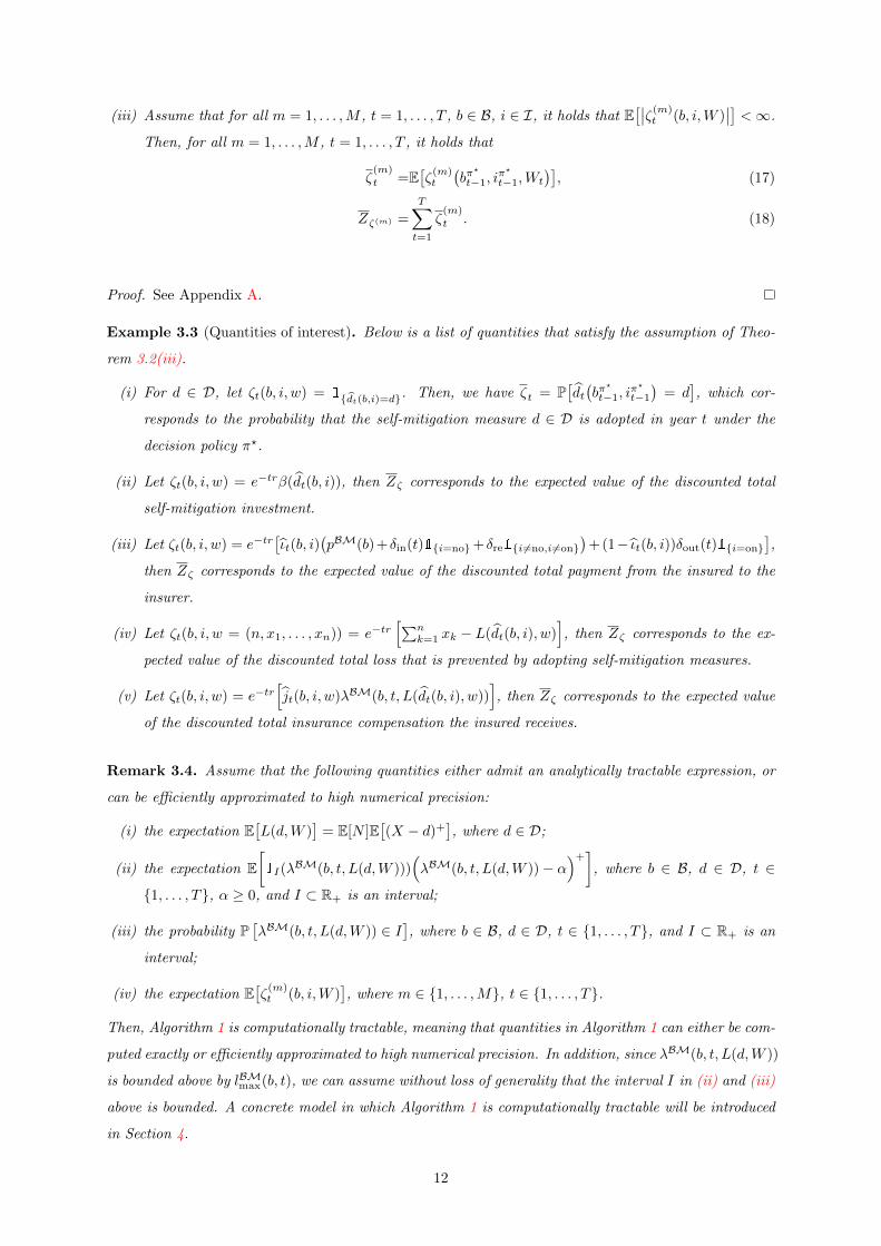
Example 3.3 (Quantities of interest). Below is a list of quantities that satisfy the assumption of Theo-

rem 3.2(iii).

(i) For d ∈ D, let ζt(b, i, w) = 1dt(b,i)=d. Then, we have ζt = P[dt(bπ?

t−1, iπ?

t−1

)= d

], which cor-

responds to the probability that the self-mitigation measure d ∈ D is adopted in year t under the

decision policy π?.

(ii) Let ζt(b, i, w) = e−trβ(dt(b, i)), then Zζ corresponds to the expected value of the discounted total

self-mitigation investment.

(iii) Let ζt(b, i, w) = e−tr[ιt(b, i)

(pBM(b)+δin(t)1i=no+δre1i6=no,i6=on

)+(1− ιt(b, i))δout(t)1i=on

],

then Zζ corresponds to the expected value of the discounted total payment from the insured to the

insurer.

(iv) Let ζt(b, i, w = (n, x1, . . . , xn)) = e−tr[∑n

k=1 xk − L(dt(b, i), w)], then Zζ corresponds to the ex-

pected value of the discounted total loss that is prevented by adopting self-mitigation measures.

(v) Let ζt(b, i, w) = e−tr[jt(b, i, w)λBM(b, t, L(dt(b, i), w))

], then Zζ corresponds to the expected value

of the discounted total insurance compensation the insured receives.

Remark 3.4. Assume that the following quantities either admit an analytically tractable expression, or

can be efficiently approximated to high numerical precision:

(i) the expectation E[L(d,W )

]= E[N ]E

[(X − d)+

], where d ∈ D;

(ii) the expectation E[1I(λ

BM(b, t, L(d,W )))(λBM(b, t, L(d,W ))− α

)+]

, where b ∈ B, d ∈ D, t ∈

1, . . . , T, α ≥ 0, and I ⊂ R+ is an interval;

(iii) the probability P[λBM(b, t, L(d,W )) ∈ I

], where b ∈ B, d ∈ D, t ∈ 1, . . . , T, and I ⊂ R+ is an

interval;

(iv) the expectation E[ζ

(m)t (b, i,W )

], where m ∈ 1, . . . ,M, t ∈ 1, . . . , T.

Then, Algorithm 1 is computationally tractable, meaning that quantities in Algorithm 1 can either be com-

puted exactly or efficiently approximated to high numerical precision. In addition, since λBM(b, t, L(d,W ))

is bounded above by lBMmax(b, t), we can assume without loss of generality that the interval I in (ii) and (iii)

above is bounded. A concrete model in which Algorithm 1 is computationally tractable will be introduced

in Section 4.

12

Algorithm 1: Dynamic Programming for Optimal Cybersecurity Provisioning

Input: B, I, D, BM, BM0, pBM, lBMdtb , lBMmax, β(·), γ(·), r,(ζ(m)(·, ·, ·)

)m=1:M

Output: V0(0,no), π?,(P ?t)t=1:T

,(P?

t

)t=0:T

,(ζ

(m)

t

)t=1:T,m=1:M

,(Zζ(m)

)m=1:M

1 VT (b, i)← 0 for all b ∈ B, i ∈ I.

2 for t = T, T − 1, . . . , 1 do

3 for b ∈ B do

4 b← BM(b, 0), b← maxBM(b, c) : c ∈ R+.

5 for b ≤ b′ ≤ b do

6 αt(b, b′)← Vt(b′, on)− Vt(b, on), Lt(b, b′)← c ∈ R+ : BM(b, c) = b′, c > αt(b, b

′).

7 for i ∈ I do

8 for d ∈ D do

9 Ht(b, i, d, 1)← Vt(b, on)−∑b≤b′≤b E

[1BM(b,λBM(b,t,L(d,W )))=b′

(λBM(b, t, L(d,W ))− αt(b, b′)

)+].

10 Ht(b, i, d, 0)← Vt(BM0(b, i)

).

11 (dt(b, i), ιt(b, i))← arg mind∈D,ι∈0,1

β(d) + ιpBM(b, t) + δin(t)1i=no,ι=1 +

δout(t)1i=on,ι=0 + δre1i 6=on,i6=no,ι=1 + E[L(d,W )

]+Ht(b, i, d, ι)

.

12 Vt−1(b, i)← e−r mind∈D,ι∈0,1

β(d) + ιpBM(b, t) + δin(t)1i=no,ι=1 +

δout(t)1i=on,ι=0 + δre1i 6=on,i6=no,ι=1 + E[L(d,W )

]+Ht(b, i, d, ι)

.

13 jt(b, i, w)← 1ιt(b,i)=11⋃b≤b′≤b Lt(b,b′)

(λBM(b, t, L(dt(b, i), w))

).

14 P ?t[(b, i)→ (b′, on)

]← 0 for all (b′, i′) ∈ B × I.

15 if ιt(b, i) = 1 then

16 for b < b′ ≤ b do

17 P ?t[(b, i)→ (b′, on)

]← P

[λBM(b, t, L(dt(b, i),W ))) ∈ Lt(b, b′)

].

18 P ?t[(b, i)→ (b, on)

]← 1−

∑b<b′≤b P

?t

[(b, i)→ (b′, on)

].

19 else

20 P ?t[(b, i)→ BM0(b, i)

]← 1.

21 P?

0(0,no)← 1, P?

0(b, i)← 0 for all (b, i) 6= (0,no).

22 for t = 1, 2, . . . , T do

23 For all (b, i) ∈ B × I, P?

t (b, i)←∑

(b′,i′)∈B×I P?t [(b′, i′)→ (b, i)]P

?

t−1(b′, i′).

24 For m = 1, . . . ,M , ζ(m)

t ←∑

(b,i)∈B×I E[ζ(m)t (b, i,W )]P

?

t−1(b, i).

25 For m = 1, . . . ,M , Zζ(m) ←∑Tt=1 ζ

(m)

t .

26 Define π? = (d?t , ι?t , j

?t )t=1:T as in (13).

27 return V0(0,no), π?,(P ?t)t=1:T

,(P?

t

)t=0:T

,(ζ

(m)

t

)t=1:T,m=1:M

,(Zζ(m)

)m=1:M

.

13

3.3 Discussion About the Pricing of the Insurance Premium

One important consideration of the cyber insurer is the choice of the annual premium. Normally, for a

fixed self-mitigation measure d ∈ D, a fixed deductible ldtb ≥ 0, and a fixed maximum compensation

lmax ≥ 0, one may consider the risk premium E[(L(d,W ) − ldtb)+ ∧ lmax]. However, these quantities

are variable in our dynamic model with the Bonus-Malus system. Moreover, the insured may choose

to change the self-mitigation measure adopted in each year, or withdraw from the cyber risk insurance

contract, thus further complicating the matter.

From the perspective of the insurer, one option is to set the premium such that the discounted expec-

tation of the difference between the total payment from the insured to the insurer and the total insurance

compensation is maximized. For simplicity, let Z ins be defined as the value of Zζ in Example 3.3(iii)

and let Zcp be defined as the value of Zζ in Example 3.3(v). Hence, Z ins − Zcp corresponds to the

discounted expectation of the difference between the total payment from the insured to the insurer and

the total insurance compensation, i.e. the insurer’s expected discounted profit, when the insured acts

optimally. Notice that Z ins − Zcp ≤ 0 due to the assumption that the insured minimizes the expected

value of the discounted total cybersecurity cost. In particular, in the absence of any regulatory mandated

requirements or external requirements, a rational insured will only consider adopting the cyber risk in-

surance if the expected value of the discounted benefit outweighs the expected value of the discounted

cost. Therefore, when the premium is set too high, the insured will choose not to adopt the cyber risk

insurance and hence Z ins = Zcp = 0. This is clearly undesirable. Another important consideration of the

insurer is the retention of customers, since the insurer needs a large homogeneous pool of risk to function.

When the premium is high, the insured may withdraw from the contract early due to a transition into a

higher Bonus-Malus level. This issue, however, can be addressed by imposing a large withdrawal penalty

δout(t), especially for later policy years (i.e. when t is close to T ). We will discuss about the problem of

setting the premium with a concrete example in Section 5.

We would like to remark that Z ins−Zcp ≤ 0 does not imply that cyber risk insurance is impractical.

These quantities are derived under the assumption that the insured follows the optimal cybersecurity

provisioning policy. In reality, the insured will typically act sub-optimally either due to the practical

complexity of the required computation being beyond the scope of decision makers or due to impartial

or incomplete information as to the severity of the risk they face. Insurers offering such products will

however build up a loss database which gives them a competitive advantage in knowing the true severity

and frequency of such events, for their potential customer base. Regulatory transparency requirements

will also play an important role in determining the profit margins that may arise if such products are

issued.

4 Modeling Cyber Loss with Truncated g-and-h Distribution

In this section, we adopt specific distributional assumptions about the random variable X, which cor-

responds to the severity of a single cyber risk event. Studies such as Maillart and Sornette (2010)

and Wheatley, Maillart, and Sornette (2016) have shown that the severity of cyber risk events have

14

heavy-tailed distributions. It is well-known that the g-and-h family introduced by Tukey (1977) contains

distributions with a wide range of skewness and kurtosis (e.g. see Figure 3 of Dutta and Perry (2006)),

which makes it suitable for modeling Operational Risk (Dutta and Perry, 2006; Peters and Sisson, 2006;

Cruz, Peters, and Shevchenko, 2015; Peters and Shevchenko, 2015). In Dutta and Perry (2006), the

following advantages of the g-and-h distribution are discussed:

• it is flexible and it fits well to real data under many different circumstances, e.g. when considering

losses of the company as a whole and when considering individual business lines or event types;

• it produces realistic estimations of the Operational Risk capital;

• it is easy to simulate random samples from.

The parameters in the g-and-h distribution can be robustly estimated based on quantiles (Xu, Iglewicz,

and Chervoneva, 2014) or L-moments (Peters, Chen, and Gerlach, 2016). Due to these properties, we

adopt the g-and-h distribution as a particular model for the severity of cyber risk events in this section.

The g-and-h distribution is a four-parameter family of distributions, given by the following definition:

X follows a g-and-h(α, ς, g, h) distribution, if

X =α+ ςYg,h(Z),

where Z ∼Normal(0, 1),

Yg,h(z) :=

exp(gz)−1

g exp(hz2

2

)if g 6= 0,

z exp(hz2

2

)if g = 0,

(19)

where α ∈ R is the location parameter, ς > 0 is the scale parameter, g ∈ R is the skewness parameter,

and h ≥ 0 is the kurtosis parameter. In this paper, we assume that the parameters α, ς, g, and h are

fixed and known. By (19), the distribution function of X is given by

FX(x) :=P[X ≤ x] = Φ(Y −1g,h

(x−ας

)), (20)

where Y −1g,h denotes the inverse function of Yg,h, and Φ denotes the distribution function of the standard

normal distribution. Even though Y −1g,h cannot be expressed analytically, it can be efficiently evaluated

using a standard root-finding procedure such as the bisection method and the Newton’s method. There-

fore, we treat Y −1g,h as a tractable function. The g-and-h distribution has the property that the m-th

moment of X exists when h < 1m (e.g. see Appendix D of Dutta and Perry (2006)). Since we consider

losses that are positively skewed and have finite expectation, from now on, we assume that g > 0 and

0 ≤ h < 1.

Since cyber losses are positive, we introduce a truncated version of the g-and-h distribution.

Definition 4.1 (Truncated g-and-h distribution). For α ∈ R, ς > 0, g > 0, h ∈ [0, 1), the random variable

X has truncated g-and-h distribution with parameters α, ς, g, h, denoted by X ∼ Tr-g-and-h(α, ς, g, h), if

X has distribution function

FX(x) := P[X ≤ x] = P[X ≤ x|X > 0], (21)

where X ∼ g-and-h(α, ς, g, h).

15

The next lemma shows some useful properties of the truncated g-and-h distribution.

Lemma 4.2. Suppose that X ∼ Tr-g-and-h(α, ς, g, h) for α ∈ R, ς > 0, g > 0, h ∈ [0, 1). Then, the

following statements hold.

(i) The distribution function of X is given by

FX(x) =

FX

(x)−FX

(0)

1−FX

(0) if x > 0,

0 if x ≤ 0,

(22)

where FX is defined in (19).

(ii) Suppose that U ∼ Uniform[0, 1], and let

XU := α+ ςYg,h

(Φ−1

(U + (1− U)FX(0)

)), (23)

then XU ∼ Tr-g-and-h(α, ς, g, h).

(iii) For any γ ≥ 0, the expectation E[(X − γ)+

]is given by:

E[(X − γ)+

]=

ς

(1− FX(0))g√

1− h

[exp

(g2

2(1− h)

)Φ

((g

1− h− Y −1

g,h

(γ−ας

))√1− h

)

− Φ(−Y −1

g,h

(γ−ας

)√1− h

)]+

(α− γ)(1− FX(γ))

1− FX(0).

(24)

Proof. See Appendix A.

Lemma 4.2(ii) allows us to efficiently generate random samples from the severity distribution FX ,

thus allowing us to approximate the distribution of quantities of interest in Example 3.3 via Monte Carlo.

Lemma 4.2(iii) shows that the Assumption (i) in Remark 3.4 is satisfied as long as the expected value of

the frequency distribution, i.e. E[N ], is also tractable. Lemma 4.2(i) provides the distribution function

that can be used to approximate the distribution function of L(d,W ). Concretely, by adopting the fast

Fourier transform (FFT) approach with exponential tilting (see e.g. Embrechts and Frei (2009); Cruz

et al. (2015)), we approximate the distribution function of L(d,W ), denoted by FL(d,W ), by a finitely

supported discrete distribution FL(d,W )(x) =∑j∈A p

(d)j 1a(d)j ≤x

, where(a

(d)j

)j∈A ⊂ R+ is a finite set

of atoms and(p

(d)j

)j∈A are the corresponding probabilities. The details of the FFT approach with expo-

nential tilting are shown in Algorithm 2. After obtaining (FL(d,W ))d∈D from Algorithm 2, the quantities

E[1I(λ

BM(b, t, L(d,W )))(λBM(b, t, L(d,W ))− α

)+]and P

[λBM(b, t, L(d,W )) ∈ I

]in Remark 3.4 can

be approximated by finite sums:

E[1I(λ

BM(b, t, L(d,W )))(λBM(b, t, L(d,W ))− α

)+] ≈∑j∈A

p(d)j 1I

(λBM

(b, t, a

(d)j

))(λBM(b, t, a

(d)j )− α

)+,

P[λBM(b, t, L(d,W )) ∈ I

]≈∑j∈A

p(d)j 1I

(λBM

(b, t, a

(d)j

)).

One may increase the granularity parameter Kgr in Algorithm 2 to increase the precision of numerical

approximation. Consequently, Assumptions (ii) and (iii) in Remark 3.4 are satisfied, and hence, Algo-

rithm 1 is tractable and efficient in this setting. In particular, Algorithm 2 only needs to be executed

once before executing Algorithm 1.

16

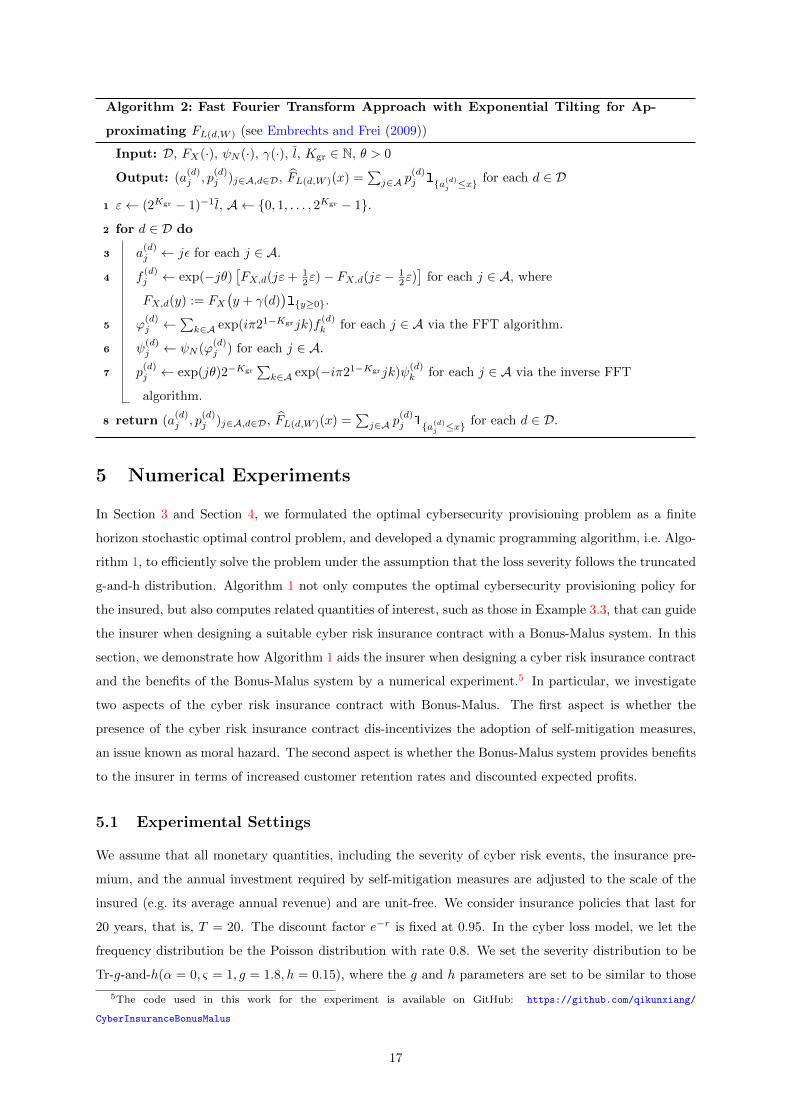
Algorithm 2: Fast Fourier Transform Approach with Exponential Tilting for Ap-

proximating FL(d,W ) (see Embrechts and Frei (2009))

Input: D, FX(·), ψN (·), γ(·), l, Kgr ∈ N, θ > 0

Output: (a(d)j , p

(d)j )j∈A,d∈D, FL(d,W )(x) =

∑j∈A p

(d)j 1a(d)j ≤x

for each d ∈ D

1 ε← (2Kgr − 1)−1l, A ← 0, 1, . . . , 2Kgr − 1.

2 for d ∈ D do

3 a(d)j ← jε for each j ∈ A.

4 f(d)j ← exp(−jθ)

[FX,d(jε+ 1

2ε)− FX,d(jε−12ε)]

for each j ∈ A, where

FX,d(y) := FX(y + γ(d)

)1y≥0.

5 ϕ(d)j ←

∑k∈A exp(iπ21−Kgrjk)f

(d)k for each j ∈ A via the FFT algorithm.

6 ψ(d)j ← ψN (ϕ

(d)j ) for each j ∈ A.

7 p(d)j ← exp(jθ)2−Kgr

∑k∈A exp(−iπ21−Kgrjk)ψ

(d)k for each j ∈ A via the inverse FFT

algorithm.

8 return (a(d)j , p

(d)j )j∈A,d∈D, FL(d,W )(x) =

∑j∈A p

(d)j 1a(d)j ≤x

for each d ∈ D.

5 Numerical Experiments

In Section 3 and Section 4, we formulated the optimal cybersecurity provisioning problem as a finite

horizon stochastic optimal control problem, and developed a dynamic programming algorithm, i.e. Algo-

rithm 1, to efficiently solve the problem under the assumption that the loss severity follows the truncated

g-and-h distribution. Algorithm 1 not only computes the optimal cybersecurity provisioning policy for

the insured, but also computes related quantities of interest, such as those in Example 3.3, that can guide

the insurer when designing a suitable cyber risk insurance contract with a Bonus-Malus system. In this

section, we demonstrate how Algorithm 1 aids the insurer when designing a cyber risk insurance contract

and the benefits of the Bonus-Malus system by a numerical experiment.5 In particular, we investigate

two aspects of the cyber risk insurance contract with Bonus-Malus. The first aspect is whether the

presence of the cyber risk insurance contract dis-incentivizes the adoption of self-mitigation measures,

an issue known as moral hazard. The second aspect is whether the Bonus-Malus system provides benefits

to the insurer in terms of increased customer retention rates and discounted expected profits.

5.1 Experimental Settings

We assume that all monetary quantities, including the severity of cyber risk events, the insurance pre-

mium, and the annual investment required by self-mitigation measures are adjusted to the scale of the

insured (e.g. its average annual revenue) and are unit-free. We consider insurance policies that last for

20 years, that is, T = 20. The discount factor e−r is fixed at 0.95. In the cyber loss model, we let the

frequency distribution be the Poisson distribution with rate 0.8. We set the severity distribution to be

Tr-g-and-h(α = 0, ς = 1, g = 1.8, h = 0.15), where the g and h parameters are set to be similar to those

5The code used in this work for the experiment is available on GitHub: https://github.com/qikunxiang/

CyberInsuranceBonusMalus

17

estimated in Dutta and Perry (2006) from real Operational Risk data (see Table 8 of Dutta and Perry

(2006)). We would like to remark that the heaviness of the tail of the loss severity distribution (i.e. the

parameter h in the truncated g-and-h distribution) determines the probability of extreme risk events

and is crucial in the computation of capital estimate (Dutta and Perry, 2006). Therefore, it is impor-

tant that we specify a realistic value of the parameter h. In Algorithm 2, we fix l = 10000, Kgr = 20,

θ = 202Kgr

= 3.0518× 10−4.

For simplicity, we consider the situation where only a single self-mitigation measure is available, that

is, D = 1. This self-mitigation measure requires an annual investment of 0.5, and has the effect of

preventing 70% of the incoming cyber risk events and decreasing the severity of the remaining events

by the 70th percentile of the severity distribution, that is, β(1) = 0.5, γ(1) = F−1X (0.7), where X ∼

Tr-g-and-h(α = 0, ς = 1, g = 1.8, h = 0.15). We consider the following simple cyber risk insurance

policy with Bonus-Malus system. Let B = −2,−1, 0, 1, and let the functions BM(bt−1, Ct) and

BM0(bt−1, it−1) be specified in Table 5.1 below.

Table 1: The BM(·, ·) and BM0(·, ·) functions that represent the Bonus-Malus update rules

BM(bt−1, Ct)Ct

= 0 > 0

bt−1

−2 −2 1

−1 −2 1

0 −1 1

1 0 1

BM0(bt−1, it−1)it−1

on off1

bt−1

−2 (−2, off1) (−1, off1)

−1 (−1, off1) (0, off1)

0 (0, off1) (0, off1)

1 (1, off1) (0, off1)

The above settings mean that when the contract is activated, the insured is migrated to level 1 in

the following policy year whenever a claim is made. When the insured does not make any claim in a

policy year, their policy is migrated downwards by one level in the following policy years until it reaches

level −2. When the contract is deactivated, if the insured’s policy is in level 1, it is migrated back to

level 0 after one year. Otherwise, the policy is migrated upwards by one level each year until it reaches

level 0. In the experiment, we let the base premium pBMbase be an adjustable parameter that is varied

between 0 and 7 with an increment of 0.005, and set the premium to be 60%, 80%, 100%, 150% of the

base premium for Bonus-Malus levels −2,−1, 0, 1, respectively. That is, we let pBM(−2, t) = 0.6pBMbase,

pBM(−1, t) = 0.8pBMbase, pBM(0, t) = pBMbase, pBM(1, t) = 1.5pBMbase for all t ∈ 1, . . . , T. We fix the

maximum compensation to be 1000, that is, lBMmax(b, t) = 1000 for all b ∈ B, t ∈ 1, . . . , T. We set the

deductible to be 0.5 for all but the last policy year, and set the deductible to be 5 for the last policy year,

that is, lBMdtb (b, t) = 0.5 for all b ∈ B, t ∈ 1, . . . , T −1 and lBMdtb (b, T ) = 5 for all b ∈ B. This is to prevent

an issue caused by the finite horizon. Since after the last policy year there is no future benefit from

the insurance policy and the insured is not incentivized to adopt the self-mitigation measure, a higher

deductible is used as the incentive in the last policy year. In addition, we let δin(t) = 0.75(t − 16)+,

δout(t) = 3 + 519 (t − 1), and δre = 3. This setting has the effect of incentivizing the insured to activate

18

0 1 2 3 4 5 6 7

base premium

0

10

20ye

ars

Without Bonus-Malus

uninsured

insured

0 1 2 3 4 5 6 7

base premium

0

10

20

ye

ars

without mitigation

with mitigation

0 1 2 3 4 5 6 7

base premium

0

10

20

ye

ars

With Bonus-Malus

uninsured

level -2

level -1

level 0

level 1

0 1 2 3 4 5 6 7

base premium

0

10

20

ye

ars

without mitigation

with mitigation

Figure 1: The retention of the cyber risk insurance policy and the expected years of adoption of the

self-mitigation measure versus the base premium.

the insurance contract early on, and dis-incentivizing withdrawal when close to the last policy year. As

a baseline for comparison, we also consider another cyber risk insurance policy without the Bonus-Malus

system, which can be modeled by letting B = 0. We fix the premium to be the base premium pBMbase,

and leave everything else identical to the policy with the Bonus-Malus system.

5.2 Results and Discussion

Figure 1 shows the expected number of years the insured’s policy spends in each of the Bonus-Malus

levels or being de-activated (uninsured) and the expected number of years the insured adopts the self-

mitigation measure. The two panels compare the cyber risk insurance policy with the Bonus-Malus

system with the one without. With the policy that does not have the Bonus-Malus system, the decisions

of the insured are completely deterministic, that is, they do not depend on the realization of losses.

When pBMbase ≤ 4.410, the optimal strategy of the insured is to purchase the cyber risk insurance every

year and only adopt the self-mitigation measure in the last policy year (due to the higher deductible in

the last policy year). When pBMbase ≥ 4.415, the optimal strategy of the insured is to never purchase the

cyber risk insurance and always adopt the self-mitigation measure. Therefore, without the Bonus-Malus

system, the issue of moral hazard is present and the insured will treat the cyber risk insurance and

the self-mitigation measure as substitute goods. On the other hand, when the Bonus-Malus system is

introduced to the cyber risk insurance policy, the decisions of the insured depend on the realization of

losses. When 4.495 ≤ pBMbase ≤ 4.930, the optimal strategy of the insured is to always purchase the cyber

risk insurance and adopt the self-mitigation measure. When 4.935 ≤ pBMbase ≤ 5.050, the optimal strategy

of the insured is to always adopt the self-mitigation measure but withdraw from the contract when

the expected future cost exceeds the expected future benefit of the insurance policy. As a result, the

retention rate, i.e. the expected proportion of years the insured activates the contract, drops when the

base premium is increased. When pBMbase ≥ 5.055, the optimal strategy of the insured is to never purchase

the cyber risk insurance and always adopt the self-mitigation measure. Hence, compared with the policy

without Bonus-Malus, the policy with Bonus-Malus incentivizes the insured to adopt the self-mitigation

measure in addition to purchasing the cyber risk insurance policy.

Figure 2 compares both the expected value of the discounted total loss prevented by the self-mitigation

measure and the expected value of the discounted profit of the insurer (defined in Section 3.3) in the

19

0 1 2 3 4 5 6 7

base premium

0

10

20p

reve

nte

d lo

ss Without Bonus-Malus

0 1 2 3 4 5 6 7

base premium

-50

0

insu

rer's p

rofit

0 1 2 3 4 5 6 7

base premium

0

10

20

pre

ve

nte

d lo

ss With Bonus-Malus

0 1 2 3 4 5 6 7

base premium

-50

0

insu

rer's p

rofit

Figure 2: The discounted total expected loss prevented by the self-mitigation measure and the discounted

expected profit of the insurer versus the base premium. Left panel: the policy without the Bonus-Malus

system. The dashed line indicates the highest base premium before the insured chooses not to purchase

cyber risk insurance. Right panel: the policy with the Bonus-Malus system. The dashed line indicates

the highest base premium before the retention drops below 100%. The dotted line indicates the highest

base premium before the insured chooses not to purchase cyber risk insurance.

two policies. The left panel of Figure 2 shows the case without Bonus-Malus. In that case, when

pBMbase ≤ 4.410, the insured will always purchase the cyber risk insurance policy but will only adopt the

self-mitigation measure in the last policy year. Hence, the discounted total expected loss prevented stays

at 0.505, while the discounted expected profit of the insurer increases as the base premium increases.

When pBMbase ≥ 4.415, the insured will not purchase the insurance policy but will always adopt the self-

mitigation measure. As a result, the discounted total expected loss prevented will be 17.183 but the

insurer will earn no profit. The most the insurer can gain before losing the insured is −10.510, when the

base premium is set to 4.410. In contrast, in the case with the Bonus-Malus system, as shown in the

right panel of Figure 2, the insurer can gain a discounted expected profit of at most −0.860 while always

retaining the insured (i.e. the insured will never withdraw from the contract), when the base premium

is set to 4.930. The insurer can gain a discounted expected profit of at most −0.006 before losing the

insured, when the base premium is set to 5.050. With both of these base premiums, the insured will

always adopt the self-mitigation measure, resulting in a discounted total expected loss prevention of

17.183.

Overall, this experiment demonstrates two benefits of the Bonus-Malus system. First, the presence

of the Bonus-Malus system incentivizes the insured to adopt the self-mitigation measure in addition

to the cyber risk insurance policy. This results in a considerable increase in the prevention of cyber

losses, which enhances the overall security of the cyberspace. Second, the Bonus-Malus system benefits

the insurer, since it allows the insurer to gain more profit from the cyber risk insurance policy while

remaining attractive to the insured.

6 Conclusion

This paper motivated the joint consideration of risk reduction and risk transfer decisions in the face of

cyber risk. We introduced a cyber risk insurance policy with a Bonus-Malus system to provide incentive

20

mechanisms to promote the adoption of cyber risk mitigation practices. We developed a model based

on the stochastic optimal control framework to analyze how a rational insured allocates funds between

risk mitigation measures and the cyber risk insurance policy. A dynamic programming-based algorithm

was then developed to efficiently solve this decision problem. A numerical experiment demonstrated

that this novel type of insurance policy can incentivize the adoption of risk mitigation measures and

can allow the insurer to profit more from the policy while remaining attractive to the insured. Future

research could investigate the effects of the risk profile, i.e. the characteristics of the loss distribution

such as the heaviness of its tail, on the effectiveness of the Bonus-Malus system and how one can tailor

Bonus-Malus-based insurance contracts for different risk profiles.

Acknowledgments

Ariel Neufeld gratefully acknowledges the financial support by his Nanyang Assistant Professorship Grant

(NAP Grant) Machine Learning based Algorithms in Finance and Insurance.

A Proofs

Proof of Theorem 3.1. In this proof, we apply dynamic programming and perform backward induction

in time to show the optimality of π?. First, one may check that d?t , ι?t are Ft−1-measurable, j?t is Ft-

measurable, and ι?t = 0, j?t = 1 = ∅ for t = 1, . . . , T . Thus, indeed π? ∈ Π. For all π = (ds, ιs, js)s=1:T ∈

Π and t ∈ 0, . . . , T, let us define Ot(π) = (ds, ιs, js)s=1:T ∈ Π as follows:(bOt(π)0 , i

Ot(π)0

):= (0,no),

for each s =1, . . . , t, let:

ds = ds, ιs = ιs, js = js,

for each s =t+ 1, . . . , T, let:

ds = ds(bOt(π)s−1 , i

Ot(π)s−1

), ιs = ιs

(bOt(π)s−1 , i

Ot(π)s−1

), js = js

(bOt(π)s−1 , i

Ot(π)s−1 ,Ws

).

(25)

By the definition above, one may check that Ot(π) ∈ Π for all π ∈ Π and t = 0, . . . , T . In particular,

when t = 0, (25) implies that O0(π) = π? for all π ∈ Π. In addition, notice that Ot+s(Ot(π)

)= Ot(π)

for all π ∈ Π and s ≥ 0.

Next, we prove the following statement by induction:

for all t = 0, . . . , T, Vt(bOt(π)t , i

Ot(π)t

)= V

Ot(π)t ≤ V πt P-a.s. for all π ∈ Π. (26)

To begin, we have by definition that OT (π) = π and VT (bπT , iπT ) = V πT = 0 P-a.s. for all π ∈ Π. Hence, (26)

holds when t = T . Now, let us suppose that for some t ∈ 1, . . . , T, it holds that Vt(bOt(π)t , i

Ot(π)t

)=

VOt(π)t ≤ V πt P-a.s. for all π ∈ Π. Let π = (ds, ιs, js)s=1:T ∈ Π be arbitrary and let Ot−1(π) :=

(ds, ιs, js)s=1:T ∈ Π. Note that (12) ensures that for every b ∈ B, i ∈ I, w ∈ W,

gt(b, i, dt(b, i), ιt(b, i), jt(b, i, w), w) + Vt(ft(b, i, dt(b, i), ιt(b, i), jt(b, i, w), w)

)= minj∈0,1

gt(b, i, dt(b, i), ιt(b, i), j, w) + Vt

(ft(b, i, dt(b, i), ιt(b, i), j, w)

).

(27)

21

Combining (27) with the definition of dt and ιt in (11), one can show that for all b ∈ B, i ∈ I, d ∈ D,

ι ∈ 0, 1, and B(W)-measurable j :W → 0, 1, it holds that

Vt−1(b, i)

=e−rE[gt(b, i, dt(b, i), ιt(b, i), jt(b, i,W ),W ) + Vt

(ft(b, i, dt(b, i), ιt(b, i), jt(b, i,W ),W )

)]≤e−rE

[gt(b, i, d, ι, j(W ),W ) + Vt

(ft(b, i, d, ι, j(W ),W )

)].

(28)

By (28), (25), the independence between Ft−1 and σ(Wt), and the induction hypothesis, it holds P-a.s.

that,

Vt−1

(bOt−1(π)t−1 , i

Ot−1(π)t−1

)=e−rE

[gt(b, i, dt(b, i), ιt(b, i), jt(b, i,W ),W )

+ Vt(ft(b, i, dt(b, i), ιt(b, i), jt(b, i,W ),W )

)]∣∣∣∣b=b

Ot−1(π)

t−1 , i=iOt−1(π)

t−1

=e−rE[gt(b

Ot−1(π)t−1 , i

Ot−1(π)t−1 , dt(b

Ot−1(π)t−1 , i

Ot−1(π)t−1 ), ιt(b

Ot−1(π)t−1 , i

Ot−1(π)t−1 ),

jt(bOt−1(π)t−1 , i

Ot−1(π)t−1 ,Wt),Wt) + Vt

(ft(b

Ot−1(π)t−1 , i

Ot−1(π)t−1 , dt(b

Ot−1(π)t−1 , i

Ot−1(π)t−1 ),

ιt(bOt−1(π)t−1 , i

Ot−1(π)t−1 ), jt(b

Ot−1(π)t−1 , i

Ot−1(π)t−1 ,Wt),Wt)

)∣∣∣∣Ft−1

]=e−rE

[gt(bOt−1(π)t−1 , i

Ot−1(π)t−1 , dt, ιt, jt,Wt

)+ Vt

(ft(bOt−1(π)t−1 , i

Ot−1(π)t−1 , dt, ιt, jt,Wt

))∣∣∣∣Ft−1

]=e−rE

[gt(bOt−1(π)t−1 , i

Ot−1(π)t−1 , dt, ιt, jt,Wt

)+ Vt

(bOt(Ot−1(π))t , i

Ot(Ot−1(π))t

)∣∣∣∣Ft−1

]=e−rE

[gt(bOt−1(π)t−1 , i

Ot−1(π)t−1 , dt, ιt, jt,Wt

)+ V

Ot−1(π)t

∣∣∣∣Ft−1

]=V

Ot−1(π)t−1 .

(29)

Now, let π = (ds, ιs, js)s=1:T ∈ Π be arbitrary and let Ot−1(π) := (ds, ιs, js)s=1:T ∈ Π. By (25), we

have that

(bπt−1, i

πt−1

)=(bOt−1(π)t−1 , i

Ot−1(π)t−1

)=(bOt(π)t−1 , i

Ot(π)t−1

)P-a.s. (30)

By (29), (27), (30), the independence between Ft−1 and σ(Wt), and the induction hypothesis, we have

22

P-a.s. that

VOt−1(π)t−1

=e−rE[

minj∈0,1

gt(b, i, dt(b, i), ιt(b, i), j,W ) + Vt

(ft(b, i, dt(b, i), ιt(b, i), j,W )

)]∣∣∣∣b=b

Ot−1(π)

t−1 , i=iOt−1(π)

t−1

≤e−rE[

minj∈0,1

gt(b, i, dt, ιt, j,W ) + Vt

(ft(b, i, dt, ιt, j,W )

)]∣∣∣∣b=b

Ot−1(π)

t−1 , i=iOt−1(π)

t−1

=e−rE[

minj∈0,1

gt(bOt−1(π)t−1 , i

Ot−1(π)t−1 , dt, ιt, j,Wt

)+ Vt

(ft(bOt−1(π)t−1 , i

Ot−1(π)t−1 , dt, ιt, j,Wt

))∣∣∣∣Ft−1

]≤e−rE

[gt(bOt−1(π)t−1 , i

Ot−1(π)t−1 , dt, ιt, jt,Wt

)+ Vt

(ft(bOt−1(π)t−1 , i

Ot−1(π)t−1 , dt, ιt, jt,Wt

))∣∣∣∣Ft−1

]=e−rE

[gt(bπt−1, i

πt−1, dt, ιt, jt,Wt

)+ Vt

(bOt(π)t , i

Ot(π)t

)∣∣∣∣Ft−1

]≤e−rE

[gt(bπt−1, i

πt−1, dt, ιt, jt,Wt

)+ V πt

∣∣∣∣Ft−1

]=V πt−1.

(31)

Combining (29) and (31), we have shown that Vt−1

(bOt−1(π)t−1 , i

Ot−1(π)t−1

)= V

Ot−1(π)t−1 ≤ V πt−1 P-a.s. for all

π ∈ Π. By induction, (26) holds for t = 0. Hence, V0

(bπ?

0 , iπ?

0

)= V π

?

0 ≤ V π0 for all π ∈ Π. Since

(bπ?

0 , iπ?

0

)= (0,no), we have V0

(bπ?

0 , iπ?

0

)= V π

?

0 = infπ∈Π Vπ0 = V0. The proof is now complete.

Proof of Theorem 3.2. To prove statement (i), it suffices to show that the two following statements hold:

(i-a) For all b ∈ B, i ∈ I, d ∈ D, ι ∈ 0, 1,

E[

minj∈0,1

gt(b, i, d, ι, j,W ) + Vt

(ft(b, i, d, ι, j,W )

)]=β(d) + ιpBM(b, t) + δin(t)1i=no,ι=1 + δout(t)1i=on,ι=0

+ δre1i 6=on,i6=no,ι=1 + E[L(d,W )

]+Ht(b, i, d, ι),

where Ht(b, i, d, ι) is defined on Line 9 and Line 10 of Algorithm 1.

(i-b) For all b ∈ B, i ∈ I, d ∈ D,

gt(b, i, d, 1, 1, w) + Vt(ft(b, i, d, 1, 1, w)

)< gt(b, i, d, 1, 0, w) + Vt

(ft(b, i, d, 1, 0, w)

)m

λBM(b, t, L(d,w)) ∈⋃

b≤b′≤b

Lt(b, b′),(32)

where b, b are defined on Line 4 of Algorithm 1, and Lt(b, b′) is defined on Line 6 of Algorithm 1.

If statements (i-a) and (i-b) hold, then one can verify that dt(b, i), ιt(b, i), jt(b, i, w) defined on Line 11

and Line 13 coincide with the definitions (11) and (12), and thus statement (i) holds as a consequence

of Theorem 3.1.

23

In statement (i-a), in the case where ι = 1, we have, by (5) and (6), that

E[

minj∈0,1

gt(b, i, d, ι, j,W ) + Vt

(ft(b, i, d, ι, j,W )

)]=E[β(d) + ιpBM(b, t) + δin(t)1i=no,ι=1 + δout(t)1i=on,ι=0 + δre1i6=on,i6=no,ι=1 + L(d,W )

]+ E

[min

j∈0,1

Vt(BM(b, jλBM(b, t, L(d,W ))), on

)− ιjλBM(b, t, L(d,W ))

]=β(d) + ιpBM(b, t) + δin(t)1i=no,ι=1 + δout(t)1i=on,ι=0 + δre1i 6=on,i6=no,ι=1 + E

[L(d,W )

]+ E

[Vt(BM(b, 0), on

)∧(Vt(BM(b, λBM(b, t, L(d,W ))), on

)− λBM(b, t, L(d,W ))

)].

Moreover, by the definition of Ht(b, i, d, ι) on Line 9, the definitions of b, b on Line 4, and the definition

of αt(b, b′) on Line 6, we have

E[Vt(BM(b, 0), on

)∧(Vt(BM(b, λBM(b, t, L(d,W ))), on

)− λBM(b, t, L(d,W ))

)]=Vt

(BM(b, 0), on

)− E

[(λBM(b, t, L(d,W ))− Vt

(BM(b, λBM(b, t, L(d,W ))), on

)+ Vt

(BM(b, 0), on

))+]

=Vt(b, on)

−∑

b≤b′≤b

E[1BM(b,λBM(b,t,L(d,W )))=b′

(λBM(b, t, L(d,W ))−

[Vt(b′, on)− Vt(b, on)

])+]

=Ht(b, i, d, 1).

Thus, statement (i-a) holds when ι = 1. In the case where ι = 0, statement (i-a) follows directly from

(5) and (6).

In statement (i-b), by (5) and (6), it holds that

gt(b, i, d, 1, 1, w) + Vt(ft(b, i, d, 1, 1, w)

)< gt(b, i, d, 1, 0, w) + Vt

(ft(b, i, d, 1, 0, w)

)m

V(BM(b, λBM(b, t, L(d,w)), on

)− λBM(b, t, L(d,w) < V

(BM(b, 0), on

).

Observe that, by the definitions of b, b on Line 4 and the definition of αt(b, b′) on Line 6, we have

c ∈ R+ : Vt(BM(b, c), on

)− c < Vt

(BM(b, 0), on

)=

⋃b≤b′≤b

c ∈ R+ : BM(b, c) = b′, c > Vt(b′, on)− Vt(b, on)

=

⋃b≤b′≤b

Lt(b, b′).

Hence, statement (i-b) holds.

Now, let us prove statement (ii). Let (b, i) ∈ B × I be fixed, let b, b be defined by Line 4, and let

Lt(b, b′) be defined by Line 6. It follows from (5) that, if ιt(b, i) = 0, then

P[(bπ?

t , iπ?

t

)= BM0(b, i)

∣∣bπ?t−1 = b, iπ?

t−1 = i]

= 1 = P ?t[(b, i)→ BM0(b, i)

],

thus showing the correctness of Line 20. Now, suppose that ιt(b, i) = 1. Then, by (5), we have that

24

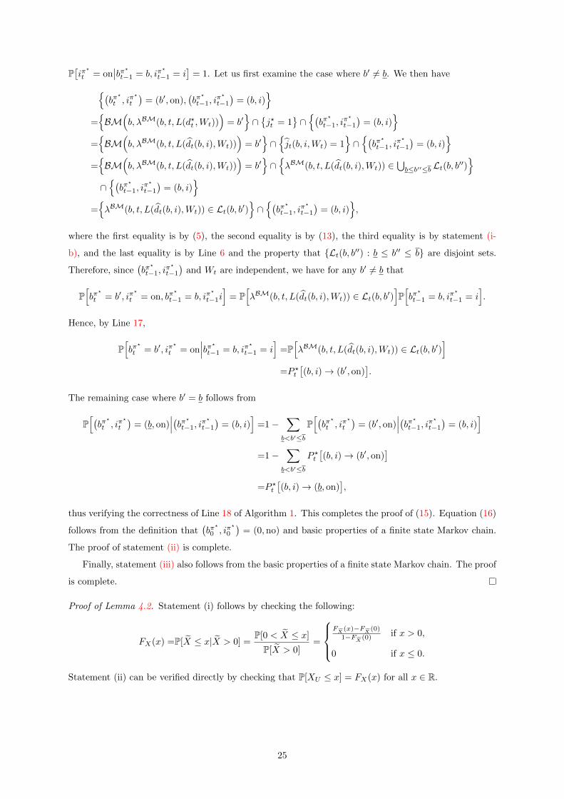
P[iπ?

t = on∣∣bπ?t−1 = b, iπ

?

t−1 = i]

= 1. Let us first examine the case where b′ 6= b. We then have(bπ?

t , iπ?

t

)= (b′, on),

(bπ?

t−1, iπ?

t−1

)= (b, i)

=BM

(b, λBM(b, t, L(d?t ,Wt))

)= b′

∩j?t = 1

∩(bπ?

t−1, iπ?

t−1

)= (b, i)

=BM

(b, λBM(b, t, L(dt(b, i),Wt))

)= b′

∩jt(b, i,Wt) = 1

∩(bπ?

t−1, iπ?

t−1

)= (b, i)

=BM

(b, λBM(b, t, L(dt(b, i),Wt))

)= b′

∩λBM(b, t, L(dt(b, i),Wt)) ∈

⋃b≤b′′≤b Lt(b, b′′)

∩(bπ?

t−1, iπ?

t−1

)= (b, i)

=λBM(b, t, L(dt(b, i),Wt)) ∈ Lt(b, b′)

∩(bπ?

t−1, iπ?

t−1

)= (b, i)

,

where the first equality is by (5), the second equality is by (13), the third equality is by statement (i-

b), and the last equality is by Line 6 and the property that Lt(b, b′′) : b ≤ b′′ ≤ b are disjoint sets.

Therefore, since(bπ?

t−1, iπ?

t−1

)and Wt are independent, we have for any b′ 6= b that

P[bπ?

t = b′, iπ?

t = on, bπ?

t−1 = b, iπ?

t−1i]

= P[λBM(b, t, L(dt(b, i),Wt)) ∈ Lt(b, b′)

]P[bπ?

t−1 = b, iπ?

t−1 = i].

Hence, by Line 17,

P[bπ?

t = b′, iπ?

t = on∣∣∣bπ?t−1 = b, iπ

?

t−1 = i]

=P[λBM(b, t, L(dt(b, i),Wt)) ∈ Lt(b, b′)

]=P ?t

[(b, i)→ (b′, on)

].

The remaining case where b′ = b follows from

P[(bπ?

t , iπ?

t

)= (b, on)

∣∣∣(bπ?t−1, iπ?

t−1

)= (b, i)

]=1−

∑b<b′≤b

P[(bπ?

t , iπ?

t

)= (b′, on)

∣∣∣(bπ?t−1, iπ?

t−1

)= (b, i)

]=1−

∑b<b′≤b

P ?t[(b, i)→ (b′, on)

]=P ?t

[(b, i)→ (b, on)

],

thus verifying the correctness of Line 18 of Algorithm 1. This completes the proof of (15). Equation (16)

follows from the definition that(bπ?

0 , iπ?

0

)= (0,no) and basic properties of a finite state Markov chain.

The proof of statement (ii) is complete.

Finally, statement (iii) also follows from the basic properties of a finite state Markov chain. The proof

is complete.

Proof of Lemma 4.2. Statement (i) follows by checking the following:

FX(x) =P[X ≤ x|X > 0] =P[0 < X ≤ x]

P[X > 0]=

FX

(x)−FX

(0)

1−FX

(0) if x > 0,

0 if x ≤ 0.

Statement (ii) can be verified directly by checking that P[XU ≤ x] = FX(x) for all x ∈ R.

25

Finally, statement (iii) can be derived from (22) as follows:

E[(X − γ)+

]=

∫ ∞γ

(x− γ)FX(dx)

=1

1− FX(0)

[∫ ∞γ

xFX(dx)− γ(1− FX(γ))

]=

ς

1− FX(0)

∫ ∞Y −1g,h( γ−ας )

Yg,h(z)Φ(dz) +(α− γ)(1− FX(γ))

1− FX(0)

=ς

1− FX(0)

1

g

∫ ∞Y −1g,h( γ−ας )

(exp(gz)− 1) exp

(hz2

2

)1√2π

exp

(−z

2

2

)dz +

(α− γ)(1− FX(γ))

1− FX(0)

=ς

1− FX(0)

1

g√

2π

[∫ ∞Y −1g,h( γ−ας )

exp

(− (1− h)z2

2+ gz

)− exp

(− (1− h)z2

2

)dz

]+

(α− γ)(1− FX(γ))

1− FX(0)

=ς

1− FX(0)

1

g√

2π

[∫ ∞Y −1g,h( γ−ας )

exp

(g2

2(1− h)

)exp

(− (1− h)

2

(z − g

1− h

)2)dz

−∫ ∞Y −1g,h( γ−ας )

exp

(− (1− h)z2

2

)dz

]+

(α− γ)(1− FX(γ))

1− FX(0)

=ς

(1− FX(0))g√

1− h

[exp

(g2

2(1− h)

)Φ

((g

1− h− Y −1

g,h

(γ−ας

))√1− h

)

− Φ(−Y −1

g,h

(γ−ας

)√1− h

)]+

(α− γ)(1− FX(γ))

1− FX(0),

where the last equality is obtained by noticing that both integrals are Gaussian integrals after a change

of variable. The proof is now complete.

References

Tridib Bandyopadhyay, Vijay S. Mookerjee, and Ram C. Rao. Why IT managers don’t go for cyber-

insurance products. Commun. ACM, 52(11):68–73, November 2009. 3

Rainer Bohme and Galina Schwartz. Modeling cyber-insurance: Towards a unifying framework. In

9th Annual Workshop on the Economics of Information Security, WEIS 2010, Harvard University,

Cambridge, MA, USA, June 7-8, 2010, 2010. 3

Jonathan Chase, Dusit Niyato, Ping Wang, Sivadon Chaisiri, and Ryan K. L. Ko. A scalable approach

to joint cyber insurance and security-as-a-service provisioning in cloud computing. IEEE Transactions

on Dependable and Secure Computing, 16(4):565–579, 2019. 4, 5

Dan Craigen, Nadia Diakun-Thibault, and Randy Purse. Defining cybersecurity. Technology Innovation

Management Review, 4(10):13–21, 2014. 2

Marcelo G. Cruz, Gareth W. Peters, and Pavel V. Shevchenko. Fundamental aspects of operational risk

and insurance analytics: A handbook of operational risk. John Wiley & Sons, 2015. 15, 16

26

Wanchun Dou, Wenda Tang, Xiaotong Wu, Lianyong Qi, Xiaolong Xu, Xuyun Zhang, and Chunhua

Hu. An insurance theory based optimal cyber-insurance contract against moral hazard. Information

Sciences, 527:576–589, 2020. 4, 5

Kabir Dutta and Jason Perry. A tale of tails: an empirical analysis of loss distribution models for

estimating operational risk capital. Technical report, Federal Reserve Bank of Boston, 2006. 15, 18

Paul Embrechts and Marco Frei. Panjer recursion versus FFT for compound distributions. Math. Methods

Oper. Res., 69(3):497–508, 2009. 16, 17

Matthias A. Fahrenwaldt, Stefan Weber, and Kerstin Weske. Pricing of cyber insurance contracts in a

network model. Astin Bull., 48(3):1175–1218, 2018. 4

Shaohan Feng, Zehui Xiong, Dusit Niyato, Ping Wang, and Amir Leshem. Evolving risk management

against advanced persistent threats in fog computing. In 2018 IEEE 7th International Conference on

Cloud Networking (CloudNet), pages 1–6, 2018. 4, 5

Emilio Granados Franco. The Global Risks Report 2020, World Economic Forum. https://www.

weforum.org/reports/the-global-risks-report-2020/, January 2020. Accessed: 2021-02-04. 1

B. B. Gupta and Omkar P. Badve. Taxonomy of dos and ddos attacks and desirable defense mechanism

in a cloud computing environment. Neural Comput. Appl., 28(12):3655–3682, December 2017. 2

Dinh Thai Hoang, Ping Wang, Dusit Niyato, and Ekram Hossain. Charging and discharging of plug-in

electric vehicles (pevs) in vehicle-to-grid (v2g) systems: A cyber insurance-based model. IEEE Access,

5:732–754, 2017. 4, 5

Martin Husak, Jana Komarkova, Elias Bou-Harb, and Pavel Celeda. Survey of attack projection, pre-

diction, and forecasting in cyber security. IEEE Communications Surveys & Tutorials, 21(1):640–660,

2019. 2

Mohammad Mahdi Khalili, Parinaz Naghizadeh, and Mingyan Liu. Designing cyber insurance policies:

The role of pre-screening and security interdependence. IEEE Transactions on Information Forensics

and Security, 13(9):2226–2239, 2018. 4, 5

Xiao Lu, Dusit Niyato, Hai Jiang, Ping Wang, and H. Vincent Poor. Cyber insurance for heterogeneous

wireless networks. IEEE Communications Magazine, 56(6):21–27, 2018a. 4

Xiao Lu, Dusit Niyato, Nicolas Privault, Hai Jiang, and Ping Wang. Managing physical layer secu-

rity in wireless cellular networks: A cyber insurance approach. IEEE Journal on Selected Areas in

Communications, 36(7):1648–1661, 2018b. 3, 4, 5

Thomas Maillart and Didier Sornette. Heavy-tailed distribution of cyber-risks. The European Physical

Journal B, 75(3):357–364, 2010. 14

Angelica Marotta, Fabio Martinelli, Stefano Nanni, Albina Orlando, and Artsiom Yautsiukhin. Cyber-

insurance survey. Computer Science Review, 24:35–61, 2017. 3

27

Steve Morgan. Cybercrime to cost the world $10.5 trillion annually by 2025. https:

//cybersecurityventures.com/cybercrime-damage-costs-10-trillion-by-2025/, Novem-

ber 2020. Accessed: 2021-02-04. 1

Ranjan Pal and Leana Golubchik. Analyzing self-defense investments in internet security under cyber-

insurance coverage. In 2010 IEEE 30th International Conference on Distributed Computing Systems,

pages 339–347, 2010. 4, 5

Ranjan Pal, Leana Golubchik, Konstantinos Psounis, and Pan Hui. Will cyber-insurance improve network

security? a market analysis. In IEEE INFOCOM 2014 - IEEE Conference on Computer Communi-

cations, pages 235–243, 2014. 4, 5

Ranjan Pal, Leana Golubchik, Konstantinos Psounis, and Pan Hui. Security pricing as enabler of cyber-

insurance a first look at differentiated pricing markets. IEEE Transactions on Dependable and Secure

Computing, 16(2):358–372, 2019. 4

Gareth W. Peters and Pavel V. Shevchenko. Advances in heavy tailed risk modeling. Wiley Handbook in

Financial Engineering and Econometrics. John Wiley & Sons, Inc., Hoboken, NJ, 2015. A handbook

of operational risk. 15

Gareth W. Peters and Scott A. Sisson. Bayesian inference, Monte Carlo sampling and operational risk.

Journal of Operational Risk, 1(3):27–50, December 2006. 15

Gareth W. Peters, Aaron D. Byrnes, and Pavel V. Shevchenko. Impact of insurance for operational risk:

is it worthwhile to insure or be insured for severe losses? Insurance Math. Econom., 48(2):287–303,

2011. 3

Gareth W. Peters, Wilson Ye Chen, and Richard H. Gerlach. Estimating quantile families of loss

distributions for non-life insurance modelling via L-moments. Risks, 4(2), 2016. 15

Gareth W. Peters, Pavel V. Shevchenko, and Ruben D. Cohen. Statistical machine learning analysis

of cyber risk data: event case studies. In Diane Maurice, Jack Freund, and David Fairman, editors,

FinTech: Growth and Deregulation, chapter 3. Risk Books, 2018a. 3

Gareth W. Peters, Pavel V. Shevchenko, and Ruben D. Cohen. Understanding cyber-risk and cyber-

insurance. In Diane Maurice, Jack Freund, and David Fairman, editors, FinTech: Growth and Dereg-

ulation, chapter 12. Risk Books, 2018b. 2, 3

Thomas Rid and Peter McBurney. Cyber-weapons. The RUSI Journal, 157(1):6–13, 2012. 2

Galina A. Schwartz and S. Shankar Sastry. Cyber-insurance framework for large scale interdependent

networks. In Proceedings of the 3rd International Conference on High Confidence Networked Systems,

HiCoNS ’14, page 145–154, New York, NY, USA, 2014. Association for Computing Machinery. 5

Nikhil Shetty, Galina Schwartz, Mark Felegyhazi, and Jean Walrand. Competitive cyber-insurance

and internet security. In Tyler Moore, David Pym, and Christos Ioannidis, editors, Economics of

Information Security and Privacy, pages 229–247. Springer US, Boston, MA, 2010. 3

28

Jinal P. Tailor and Ashish D. Patel. A comprehensive survey: ransomware attacks prevention, monitoring

and damage control. International Journal of Scientific Research, 4:2321–2705, 06 2017. 2

John W Tukey. Exploratory data analysis, volume 2. Reading, MA: Addison-Wesley, 1977. 15

Spencer Wheatley, Thomas Maillart, and Didier Sornette. The extreme risk of personal data breaches

and the erosion of privacy. The European Physical Journal B, 89(1):1–12, 2016. 14

Maochao Xu and Lei Hua. Cybersecurity insurance: Modeling and pricing. North American Actuarial

Journal, 23(2):220–249, 2019. 4

Yihuan Xu, Boris Iglewicz, and Inna Chervoneva. Robust estimation of the parameters of g-and-h

distributions, with applications to outlier detection. Computational Statistics & Data Analysis, 75:66

– 80, 2014. 15

Zichao Yang and John C.S. Lui. Security adoption and influence of cyber-insurance markets in hetero-

geneous networks. Performance Evaluation, 74:1 – 17, 2014. 5

Adam Young and Moti Yung. Cryptovirology: extortion-based security threats and countermeasures. In

Proceedings 1996 IEEE Symposium on Security and Privacy, pages 129–140, 1996. 2

Rui Zhang and Quanyan Zhu. Optimal cyber-insurance contract design for dynamic risk management

and mitigation. Preprint arXiv:1804.00998, 2018. 5

Rui Zhang, Quanyan Zhu, and Yezekael Hayel. A bi-level game approach to attack-aware cyber insurance

of computer networks. IEEE Journal on Selected Areas in Communications, 35(3):779–794, 2017. 5

29