A bioinformatic analysis of the role of mitochondrial biogenesis in human pathologies Robert Bentham A dissertation submitted in partial fulfillment of the requirements for the degree of Doctor of Philosophy of University College London. Department of Cell and Developmental Biology University College London Monday 11 th July, 2016

Welcome message from author
This document is posted to help you gain knowledge. Please leave a comment to let me know what you think about it! Share it to your friends and learn new things together.
Transcript

A bioinformatic analysis of the role ofmitochondrial biogenesis in human
pathologies
Robert Bentham
A dissertation submitted in partial fulfillment
of the requirements for the degree of
Doctor of Philosophy
of
University College London.
Department of Cell and Developmental Biology
University College London
Monday 11th July, 2016

Declaration
I, Robert Bentham, confirm that the work presented in this thesis is my own. Where
information has been derived from other sources, I confirm that this has been indicated
in the work.
July, 2016
Robert Bentham
2

Abstract
Disease states are often associated with radical rearrangements of cellular metabolism;
suggesting the transcriptome underlying these changes follows a distinctive pattern.
Identification of these patterns is complicated by the hugely heterogeneous nature
of these diseases, such as cancer, and the patterns remain hidden within noise of
large datasets. A new biclustering algorithm called Massively Correlating Biclustering
(MCbiclust) was developed to identify these patterns. Taking a large gene set such as
those known to be associated with the mitochondria, samples are selected in which
these genes are highly correlated. Rigorous benchmarking of this method with other
biclustering methods on synthetic gene expression data and an E. coli data set show it to
be superior in finding these patterns.
This method was used to identify the role mitochondrial biogenesis plays in cancer;
applied on the Cancer Cell Line Encyclopedia (CCLE) it identified differences in
mitochondrial function based on the different tissue of origin of the cell line. In patient
breast tumour samples a change in mitochondrial function was identified and linked to
differences in known breast cancer subtypes.
Breast cancer cell lines were identified that matched this pattern. Experimen-
tally testing these cell lines confirming the significant difference in gene expression
expected and also showed significant changes in mitochondrial function demonstrated
by measurements in oxygen consumption, proteomics and metabolomics.
MCbiclust has been developed into an R package. Using this method, new cancer
subtypes can be identified, based on fundamental changes to known pathways. The
benefit is twofold: first to increase understanding of these complex systems and second
to guide treatment using drug compounds known to target these pathways. The methods
described here while applied to cancer and mitochondria, are versatile and can be applied
to any large dataset of gene expression measurements.
3

Acknowledgements
First, I would like to express my utmost thanks to my supervisors Professor Gyorgy
Szabadkai and Dr. Kevin Bryson; without their support, guidance, expert knowledge,
kindness, and access to the Department of Computer Science coffee machine, this work
could have never been completed.
I would like to thank the British Heart Foundation for funding my research and
giving me the financial backing that I vitally needed.
I would like to thank Professor Michael Duchen and everyone involved with the
Szabadkai Lab both past and present: Drs. Jose Vicencio, Zhi Yao, Ronan Astin, Will
Kotiadis, Thomas Blacker and Nicoletta Plotegher for their patience in helping me with
experimental techniques and welcoming me to the lab. I would also like to thank my
fellow PhD students: Julia Hill, Jenny Sharpe, Pedro Dias, Stephanie Sundier, Neta
Amior and Gauri Bhosale, all of whom helped me enormously and better than that
made the entire experience fun! I would also like to thank Sam Ranasinghe for his
work in maintaining much of the equipment in the lab and teaching me how to use the
microscopes.
I would like to thank everyone involved in CoMPLEX, a department whose exis-
tence made possible my transition from mathematics to biological research, and without
which I certainly would never have embarked on this work.
I thank my fellow Szabadkai lab PhD student Michella Menegollo at the University
of Padova who greatly contributed to the experimental work of this project, and Dr.
Mariia Yuneva of the Crick Institute for her collaboration and help on this project.
Finally, I would have never been able to complete this huge undertaking without
the constant support of my family and friends.
4

List of my publications
The following publications were produced during my PhD but not related to the topic of
this thesis:
Astin, R., Bentham, R., Djafarzadeh, S., Horscroft, J. A., Kuc, R. E., Leung, P. S.,
Skipworth, J. R., Vicencio, J. M., Davenport, A. P., Murray, A. J. et al. (2013), ‘No
evidence for a local renin-angiotensin system in liver mitochondria’, Scientific reports
3.
Tosatto, A., Sommaggio, R., Kummerow, C., Bentham, R. B., Blacker, T. S., Berecz,
T., Duchen, M. R., Rosato, A., Bogeski, I., Szabadkai, G. et al. (2016), ‘The mito-
chondrial calcium uniporter regulates breast cancer progression via hif-1a’, EMBO
molecular medicine 8(5), 569–585.
5

Contents
Declaration 2
Abstract 3
Acknowledgements 4
List of my publications 5
List of Figures 10
List of Tables 13
Abbreviations 15
1 Introduction 19
1.1 Mitochondria . . . . . . . . . . . . . . . . . . . . . . . . . . . . . . . 19
1.1.1 The basics of mitochondrial function . . . . . . . . . . . . . . 19
1.1.2 The role of mitochondria in apoptosis and their evolutionary
history . . . . . . . . . . . . . . . . . . . . . . . . . . . . . . 21
1.2 Mitochondrial heterogeneity . . . . . . . . . . . . . . . . . . . . . . . 23
1.2.1 The mitochondrial proteome . . . . . . . . . . . . . . . . . . . 23
1.2.2 Variation across tissues and in disease . . . . . . . . . . . . . . 25
1.3 Mechanisms of regulation of the mitochondria . . . . . . . . . . . . . . 27
1.3.1 Epigenetics . . . . . . . . . . . . . . . . . . . . . . . . . . . . 28
1.3.2 Mitochondrial degradation, quality control and turnover . . . . 29
1.3.3 Mitochondrial biogenesis . . . . . . . . . . . . . . . . . . . . . 34
6

1.3.4 The transcription factor network underlying mitochondria bio-
genesis . . . . . . . . . . . . . . . . . . . . . . . . . . . . . . 38
1.4 Mitochondria and disease . . . . . . . . . . . . . . . . . . . . . . . . . 52
1.4.1 Cancer . . . . . . . . . . . . . . . . . . . . . . . . . . . . . . 52
1.4.2 Heart disease . . . . . . . . . . . . . . . . . . . . . . . . . . . 56
1.4.3 Neurodegeneration, diabetes and ageing . . . . . . . . . . . . . 57
1.5 Investigating the regulation of mitochondria . . . . . . . . . . . . . . . 60
1.5.1 Experimental methods . . . . . . . . . . . . . . . . . . . . . . 60
1.5.2 Bioinformatics . . . . . . . . . . . . . . . . . . . . . . . . . . 61
1.6 Overview and aims of thesis . . . . . . . . . . . . . . . . . . . . . . . 68
2 A novel biclustering algorithm 70
2.1 Introduction . . . . . . . . . . . . . . . . . . . . . . . . . . . . . . . . 70
2.2 Massively correlated biclustering (MCbiclust) . . . . . . . . . . . . . . 74
2.2.1 Defining a method of measuring bicluster quality . . . . . . . . 75
2.2.2 A stochastic greedy search for biclusters . . . . . . . . . . . . . 78
2.2.3 Pruning the bicluster . . . . . . . . . . . . . . . . . . . . . . . 79
2.2.4 Extending the bicluster . . . . . . . . . . . . . . . . . . . . . . 80
2.2.5 Analysing the bicluster . . . . . . . . . . . . . . . . . . . . . . 81
2.2.6 Thresholding the bicluster . . . . . . . . . . . . . . . . . . . . 83
2.2.7 Methods for dealing with multiple runs . . . . . . . . . . . . . 84
2.3 Benchmarking of massively correlated biclustering on a simulated dataset 87
2.3.1 Generation of artificial data . . . . . . . . . . . . . . . . . . . 87
2.3.2 Means of comparison between different biclustering methods . 89
2.3.3 Biclustering methods . . . . . . . . . . . . . . . . . . . . . . . 92
2.3.4 Comparison of different biclustering methods . . . . . . . . . . 95
2.4 Case study: Escherichia coli expression data . . . . . . . . . . . . . . . 98
2.4.1 Rationale . . . . . . . . . . . . . . . . . . . . . . . . . . . . . 98
2.4.2 Finding the number of distinct biclusters . . . . . . . . . . . . 99
2.4.3 Analysis of different bicluster patterns . . . . . . . . . . . . . . 101
2.4.4 Analysis of random probe sets . . . . . . . . . . . . . . . . . . 105
2.5 Conclusion . . . . . . . . . . . . . . . . . . . . . . . . . . . . . . . . 107
7

3 Bioinformatic analysis of mitochondrial biogenesis in disease 109
3.1 Introduction . . . . . . . . . . . . . . . . . . . . . . . . . . . . . . . . 109
3.1.1 Hypertrophic Cardiomyopathy (HCM) . . . . . . . . . . . . . . 110
3.1.2 Cancer cell lines . . . . . . . . . . . . . . . . . . . . . . . . . 112
3.2 Bioinformatic analysis of mitochondrial biogenesis in hypertrophic
cardiomyopathy . . . . . . . . . . . . . . . . . . . . . . . . . . . . . . 113
3.2.1 The data . . . . . . . . . . . . . . . . . . . . . . . . . . . . . . 113
3.2.2 Silhouette plots and ranking the samples . . . . . . . . . . . . . 114
3.2.3 Comparing the biclusters . . . . . . . . . . . . . . . . . . . . . 116
3.3 Bioinformatic analysis of mitochondrial biogenesis in cancer cell lines . 124
3.3.1 The data . . . . . . . . . . . . . . . . . . . . . . . . . . . . . . 124
3.3.2 Silhouette plots and comparison . . . . . . . . . . . . . . . . . 124
3.3.3 Understanding the biclusters . . . . . . . . . . . . . . . . . . . 125
3.3.4 Copy number differences . . . . . . . . . . . . . . . . . . . . . 129
3.3.5 Pharmacology differences . . . . . . . . . . . . . . . . . . . . 133
3.4 Conclusion . . . . . . . . . . . . . . . . . . . . . . . . . . . . . . . . 136
4 Bioinformatic analysis of mitochondrial biogenesis in breast cancer 140
4.1 Introduction . . . . . . . . . . . . . . . . . . . . . . . . . . . . . . . . 140
4.1.1 Breast cancer . . . . . . . . . . . . . . . . . . . . . . . . . . . 140
4.1.2 Intrinsic subtypes of breast cancer . . . . . . . . . . . . . . . . 143
4.1.3 Examining mitochondrial biogenesis in breast cancer . . . . . . 147
4.2 Bioinformatic analysis of a breast cancer sample dataset . . . . . . . . 147
4.2.1 Using a new gene set . . . . . . . . . . . . . . . . . . . . . . . 147
4.2.2 The data . . . . . . . . . . . . . . . . . . . . . . . . . . . . . . 150
4.2.3 Finding a mitochondrial related bicluster in a breast cancer dataset150
4.2.4 Mutational alterations behind the bicluster . . . . . . . . . . . . 156
4.3 Identification of a similar bicluster in a breast cancer cell line dataset . . 160
4.3.1 The data . . . . . . . . . . . . . . . . . . . . . . . . . . . . . . 160
4.3.2 Point Scoring algorithm . . . . . . . . . . . . . . . . . . . . . 161
4.3.3 Selecting breast cancer cell lines . . . . . . . . . . . . . . . . . 162
8

4.4 Experimental study of mitochondrial function in different breast cancer
cell lines . . . . . . . . . . . . . . . . . . . . . . . . . . . . . . . . . . 164
4.4.1 Methodology . . . . . . . . . . . . . . . . . . . . . . . . . . . 164
4.4.2 Results . . . . . . . . . . . . . . . . . . . . . . . . . . . . . . 170
4.5 Conclusion . . . . . . . . . . . . . . . . . . . . . . . . . . . . . . . . 177
5 Conclusions 181
Bibliography 185
Appendices 221
A MCbiclust - an R package for massively correlated biclustering 221
A.1 About . . . . . . . . . . . . . . . . . . . . . . . . . . . . . . . . . . . 221
A.2 Installation . . . . . . . . . . . . . . . . . . . . . . . . . . . . . . . . 221
A.3 Example workflow . . . . . . . . . . . . . . . . . . . . . . . . . . . . 222
B Gene set enrichment result tables 227
C Nanostring gene set 270
D Materials 274
9

List of Figures
1.1 The basic stucture of a mitochondrion . . . . . . . . . . . . . . . . . . 20
1.2 Oxidative phoshporylation (OXPHOS) system and citric acid cycle
within the mitochondrion. . . . . . . . . . . . . . . . . . . . . . . . . . 22
1.3 Variation of protein abundance of mitochondrial genes. . . . . . . . . . 25
1.4 Methods of quality control . . . . . . . . . . . . . . . . . . . . . . . . 30
1.5 Simplified overview of the mitochondrial biogenesis transcription factor
network . . . . . . . . . . . . . . . . . . . . . . . . . . . . . . . . . . 38
1.6 Regulation of peroxisome proliferator-activated receptor gamma coacti-
vator 1-a (PGC-1a) . . . . . . . . . . . . . . . . . . . . . . . . . . . 46
1.7 Mitochondrial dysfunction in the hallmarks of ageing and cancer . . . . 53
1.8 The Warburg effect . . . . . . . . . . . . . . . . . . . . . . . . . . . . 54
1.9 An RNA sequencing (RNA-seq) experiment . . . . . . . . . . . . . . . 63
2.1 Two models of mitochondrial biogenesis in gene expression data . . . . 71
2.2 Different types of biclusters . . . . . . . . . . . . . . . . . . . . . . . . 72
2.3 Work pipeline of Massively Correlating Biclustering (MCbiclust) for a
single run . . . . . . . . . . . . . . . . . . . . . . . . . . . . . . . . . 76
2.4 Work pipeline of MCbiclust for multiple runs . . . . . . . . . . . . . . 77
2.5 A visual explanation of silhouette widths . . . . . . . . . . . . . . . . . 86
2.6 Pipeline used to compare different biclustering algorithms on the syn-
thetic data . . . . . . . . . . . . . . . . . . . . . . . . . . . . . . . . . 91
2.7 Jaccard index matrix from two different discovered MCbiclust patterns
compared to the same synthetic bicluster . . . . . . . . . . . . . . . . . 94
2.8 Principal component plots from synthetic data results. . . . . . . . . . . 95
10

2.9 Receiver operator characteristics (ROC) plots comparing different bi-
clustering methods - part 1. . . . . . . . . . . . . . . . . . . . . . . . . 96
2.9 ROC plots comparing different biclustering methods - part 2 . . . . . . 97
2.10 Heat map of correlation matrix of gene-probe correlation vectors from
running MCbiclust on E. coli dataset . . . . . . . . . . . . . . . . . . . 100
2.11 Output from silhouette width analysis on E. coli data. . . . . . . . . . . 101
2.12 The different regulation of intergenic and non-intergenic regions in the
E. coli dataset . . . . . . . . . . . . . . . . . . . . . . . . . . . . . . . 103
2.13 Biclustering results of E. coli show the E3 pattern linked to genome
position . . . . . . . . . . . . . . . . . . . . . . . . . . . . . . . . . . 104
2.14 Analysing random probe sets within the E. coli dataset . . . . . . . . . 106
3.1 Possible clinical outcomes of hypertrophic cardiomyopathy (HCM) . . 111
3.2 Silhouette analysis of two sets of runs in the HCM data. . . . . . . . . . 115
3.3 The first principal component (PC1) plots of two sets of runs in the
HCM data. . . . . . . . . . . . . . . . . . . . . . . . . . . . . . . . . . 116
3.4 Average mitochondrial expression plot of Mito.1 pattern . . . . . . . . 117
3.5 Silhouette analysis set of runs in the HCM data on mitochondrial genes
without the controls. . . . . . . . . . . . . . . . . . . . . . . . . . . . 117
3.6 PC1 plots of biclusters from set of runs in the HCM data on the mito-
chondrial genes without controls. . . . . . . . . . . . . . . . . . . . . . 118
3.7 Comparison plot of the correlation vectors from the 5 biclusters found
in the HCM data. . . . . . . . . . . . . . . . . . . . . . . . . . . . . . 119
3.8 Heat map showing a module of similarly regulated mitochondrial genes
in the correlation vector values . . . . . . . . . . . . . . . . . . . . . . 122
3.9 Silhouette analysis of two sets of runs in the Cancer Cell Line Encyclo-
pedia (CCLE) data. . . . . . . . . . . . . . . . . . . . . . . . . . . . . 125
3.10 Comparison plot of the correlation vectors from the 3 found biclusters
in the CCLE data. . . . . . . . . . . . . . . . . . . . . . . . . . . . . . 126
3.11 PC1 plots of two biclusters from set of runs in the CCLE data . . . . . 127
3.12 PC1 plots of a bicluster from set of runs in the CCLE data . . . . . . . 128
11
3.13 CCLE biclustering significant copy number differences between upper
and lower forks in Mito.CV1 . . . . . . . . . . . . . . . . . . . . . . . 133
3.14 CCLE biclustering significant copy number differences between upper
and lower forks in Random.CV1 and Random.CV2 . . . . . . . . . . . 134
3.15 CCLE biclustering significant pharmacological differences between
upper and lower forks . . . . . . . . . . . . . . . . . . . . . . . . . . . 137
4.1 The PAM50 subtypes and commonly associated clinical phenotypes . . 146
4.2 The protein-protein interaction (PPI) network of mitochondrial gene
immature colon carcinoma transcript 1 (ICT1) . . . . . . . . . . . . . . 149
4.3 Silhouette analysis of three sets of runs in the breast cancer data. . . . . 151
4.4 Comparison plot of the correlation vectors from the 7 biclusters found
in the breast cancer data. . . . . . . . . . . . . . . . . . . . . . . . . . 152
4.5 PC1 plots of 4 biclusters found in the breast cancer data . . . . . . . . 153
4.6 Copy number alterations between upper/lower and luminal A/B in the
ICT1.CV1 bicluster . . . . . . . . . . . . . . . . . . . . . . . . . . . . 158
4.7 Comparison between the point score values and PC1 of the ICT1.CV1
bicluster . . . . . . . . . . . . . . . . . . . . . . . . . . . . . . . . . . 162
4.8 Comparison between the nanostring score values and PC1 the ICT1.CV1
bicluster . . . . . . . . . . . . . . . . . . . . . . . . . . . . . . . . . . 172
4.9 Representative western blot of breast cancer cell lines . . . . . . . . . . 174
4.10 Summary of the western blots analysing protein levels of different
electron transport chain (ETC) complexes . . . . . . . . . . . . . . . . 175
4.11 Differing oxygen consumption rates in the cancer cell lines . . . . . . . 176
4.12 Results of mass spectrometry of cancer cell lines from glucose labelling 178
4.13 Results of mass spectrometry of cancer cell lines from glutamine labelling179
A.1 Heatmap of correlation matrix before and after selection of genes. . . . 224
A.2 PC1 of the first 100 samples in a bicluster found in the CCLE data . . . 226
12

List of Tables
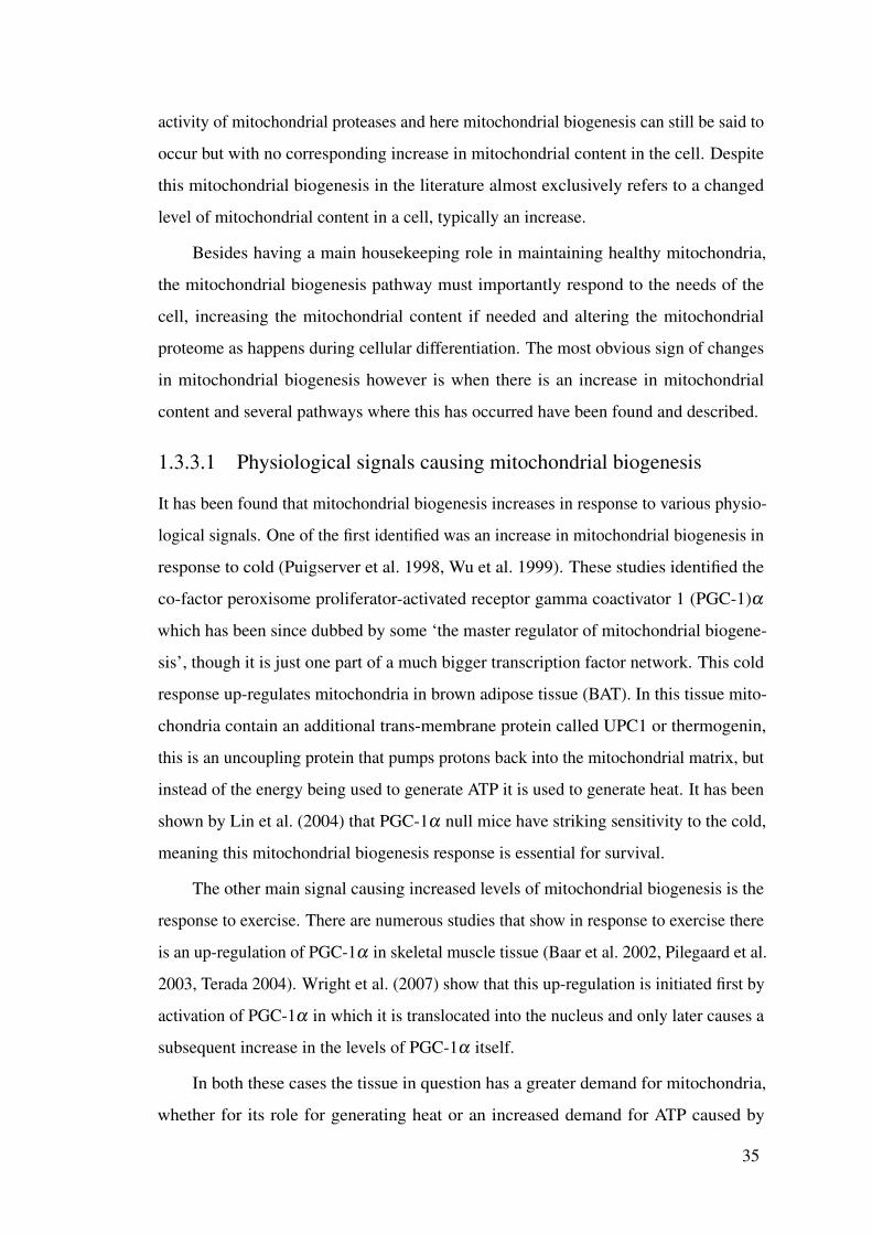
1.1 Transcription factors and coregulators in the mitochondrial biogenesis
network. . . . . . . . . . . . . . . . . . . . . . . . . . . . . . . . . . . 49
1.2 Experimental methods for measuring regulation of mitochondrial bio-
genesis and function. . . . . . . . . . . . . . . . . . . . . . . . . . . . 62
2.1 Summary of the different biclustering algorithms compared . . . . . . . 93
2.2 Comparison statistics of different biclustering methods . . . . . . . . . 98
3.1 Mitochondrial co-regulated gene module identified in two different
biclusters . . . . . . . . . . . . . . . . . . . . . . . . . . . . . . . . . 121
3.2 Significant copy number change regions for the Mito.CV1 pattern be-
tween upper and lower forks . . . . . . . . . . . . . . . . . . . . . . . 130
3.3 Significant copy number change regions for the Random.CV1 pattern
between upper and lower forks . . . . . . . . . . . . . . . . . . . . . . 132
3.4 Significant copy number change regions for the Random.CV2 pattern
between upper and lower forks . . . . . . . . . . . . . . . . . . . . . . 133
3.5 Significant pharmacological high concentration effect level changes in
the Mito.CV1 bicluster pattern . . . . . . . . . . . . . . . . . . . . . . 135
3.6 Significant pharmacological high concentration effect level changes in
the Random.CV1 bicluster pattern . . . . . . . . . . . . . . . . . . . . 136
3.7 Significant pharmacological high concentration effect level changes in
the Random.CV2 bicluster pattern . . . . . . . . . . . . . . . . . . . . 136
4.1 Previously found significant terms related to mitochondria and ribosome 148
4.2 Significant mitochondrial related gene ontology (GO) terms in biclusters
found in the breast cancer dataset. . . . . . . . . . . . . . . . . . . . . 154
13

4.3 Differences in average expression in significant mitochondria associated
GO terms between the upper and lower fork samples in bicluster ICT1.CV1156
4.4 Significant regions of copy number alterations between luminal A and
lower fork samples and luminal B and upper fork samples. . . . . . . . 159
4.5 Somatic mutations that are significant between the upper/lower fork and
luminal A/B samples . . . . . . . . . . . . . . . . . . . . . . . . . . . 160
4.6 Point Scores for breast cancer cell lines . . . . . . . . . . . . . . . . . 163
4.7 Groups of genes selected for the nanostring gene set . . . . . . . . . . . 171
4.8 Nanostring scores for breast cancer cell lines . . . . . . . . . . . . . . . 173
B.1 E. coli bicluster E1 gene enrichment results . . . . . . . . . . . . . . . 227
B.2 E. coli bicluster E2 gene enrichment results . . . . . . . . . . . . . . . 230
B.3 E. coli bicluster E3 gene enrichment results . . . . . . . . . . . . . . . 230
B.4 HCM bicluster Mito.1 gene enrichment results . . . . . . . . . . . . . . 233
B.5 HCM bicluster Random.1 gene enrichment results . . . . . . . . . . . . 237
B.6 HCM bicluster Mitonc.1 gene enrichment results . . . . . . . . . . . . 240
B.7 HCM bicluster Mitonc.2 gene enrichment results . . . . . . . . . . . . 243
B.8 HCM bicluster Mitonc.3 gene enrichment results . . . . . . . . . . . . 244
B.9 CCLE bicluster Mito.CV1 gene enrichment results . . . . . . . . . . . 246
B.10 CCLE bicluster Random.CV1 gene enrichment results . . . . . . . . . 248
B.11 CCLE bicluster Random.CV2 gene enrichment results . . . . . . . . . 251
B.12 Top 200 of 651 significant terms for ICT1 related gene set . . . . . . . 254
B.13 Breast cancer bicluster Mito.CV1 gene enrichment results . . . . . . . . 258
B.14 Breast cancer bicluster Mito.CV2 gene enrichment results . . . . . . . . 260
B.15 Breast cancer bicluster Mito.CV3 gene enrichment results . . . . . . . . 263
B.16 Breast cancer bicluster ICT1.CV1 gene enrichment results . . . . . . . 266
C.1 All the genes measured in the nanostring gene set . . . . . . . . . . . . 270
D.1 Table of materials used in this thesis . . . . . . . . . . . . . . . . . . . 274
14

Abbreviations
ADP adenosine diphosphate.
ANOVA analysis of variance.
ATP adenosine triphosphate.
BAT brown adipose tissue.
cAMP cyclic adenosine monophosphate.
CCLE Cancer Cell Line Encyclopedia.
cDNA complementary DNA.
CoRR co-location for redox regulation.
CREB cAMP response element binding protein.
DBD DNA-binding domain.
ER estrogen receptor.
ERR estrogen-related receptor.
ERRa estrogen-related receptor a .
ERRb estrogen-related receptor b .
ERRg estrogen-related receptor g .
ETC electron transport chain.
FABIA Factor Analysis for Bicluster Acquisition.
15

FPR false positive rate.
GABP GA-binding protein.
GISTIC genomic identification of significant targets in cancer.
GO gene ontology.
GSEA gene set enrichment analysis.
HCM hypertrophic cardiomyopathy.
HER2 human epidermal growth factor receptor 2.
ICD implantable cardioverter-defibrillator.
ICT1 immature colon carcinoma transcript 1.
KEGG Kyoto encyclopedia of genes and genomes.
MCbiclust Massively Correlating Biclustering.
MEF2A myocyte-specific enhancer factor 2A.
MELAS mitochondrial encephalomyopathy, lactic acidosis, and stroke-like episodes.
miRNA micro RNA.
mRNA messenger RNA.
mtDNA mitochondrial DNA.
mTOR mammalian target of rapamycin.
NAD+ nicotinamide adenine dinucleotide (oxidised).
NADH nicotinamide adenine dinucleotide (reduced).
NCoR1 nuclear receptor corepressor 1.
NPI Nottingham prognostic index.
16

NRF-1 nuclear respiration factor 1.
NRF-2 nuclear respiration factor 2.
OXPHOS oxidative phoshporylation.
PAM prediction analysis for microarrays.
PC1 the first principal component.
PCA principal component analysis.
PD Parkinson’s disease.
PGC peroxisome proliferator-activated receptor gamma coactivator.
PGC-1 peroxisome proliferator-activated receptor gamma coactivator 1.
PGC-1a peroxisome proliferator-activated receptor gamma coactivator 1-a .
PPAR peroxisome proliferator-activated receptor.
PPAR d peroxisome proliferator-activated receptor d .
PPARa peroxisome proliferator-activated receptor a .
PPARg peroxisome proliferator-activated receptor g .
PPI protein-protein interaction.
PR progesterone receptor.
PRC PGC-1 related coactivator.
q-PCR quantitative polymerase chain reaction.
RMA robust multi-array average.
ROC receiver operator characteristics.
ROR risk of recurrence.
ROS reactive oxygen species.
17

RPKM reads per kilobase per million mapped reads.
SNP single nucleotide polymorphism.
SSD signal sensing domain.
TAD trans-activating domain.
TCA tricarboxylic acid.
TF transcription factor.
TFAM transcription factor A mitochondrial.
TPR true positive rate.
tRNA transfer RNA.
YY1 Yin Yang 1.
18

Chapter 1
Introduction
1.1 Mitochondria
1.1.1 The basics of mitochondrial functionMitochondria are compartments within the cell, cellular organelles, separated from the
rest of the cell by an outer membrane and divided within itself by an inner membrane.
This double membrane organelle thus has two subspaces, the inter-membrane space and
the mitochondrial matrix.
The basic structure of a mitochondrion is given in Figure 1.1 and is remarkably
complex. The inner membrane contains numerous folds called cristae that are utilised to
maximise its surface area used for performing important biological reactions.
Inside the mitochondrial matrix there are multiple copies of mitochondrial DNA
(mtDNA) as well as mitochondrial ribosomes for the protein synthesis of 13 protein
encoding genes and 22 transfer RNAs (tRNAs). This is a system for the synthesis of
specific proteins that is separate from the normal protein synthesis pathway in the nucleus
and cytosolic ribosomes. Numerous proteins assemble into pores in both the inner
and outer membrane and are involved in the transport of biological molecules across
the membranes, composing part of a vast cellular transport and signalling networks.
In addition to the complexity of mitochondrial structure, their organisation is highly
regulated, with mitochondria fusing and dividing with the many others, forming complex
networks.
Regarding the complexity of the structure and organisation of mitochondria, it
is perhaps surprising that the function they are widely known for is merely energy
production. This suggests that provision of energy for the cell is not a simple process,
19

Figure 1.1: The basic stucture of a mitochondrion, electron microscope image taken from TheHistology Guide University of Leeds (2016).
and depends on many forms of regulation.
The standard eukaryotic cell has a basic energetic problem; the transport and storage
of energy. The cell can use energy from catabolism, the breaking down of organic matter
through metabolic pathways. However the processes that use this energy in the cell
(e.g. the synthesis of DNA, RNA and proteins as well as mechanical, signalling and
transport functions) will not always take place at either the same rate as the energy made
available by catabolism or in the same physical location. Thus for this release of energy
from catabolism to be useful to the cell, it must be able to be stored and transported
to where it is needed. This is the role adenosine triphosphate (ATP) play in the cell
and mitochondria are the organelles primarily responsible for its production. Therefore
mitochondria need to be regulated to adjust the rate of ATP production and meet the
energetic needs of the cell.
ATP stores energy in the form of chemical potential energy, the molecule contains
two phosphoanhydride bonds which when cleaved through the process of hydrolysis
release energy. This energy released then can be used to drive numerous reactions
throughout the cell.
The method mitochondria use to create ATP is through a process called oxidative
phoshporylation (OXPHOS). The process starts within the citric acid cycle (also known
20

as the tricarboxylic acid (TCA) cycle), a 9 step process that converts pyruvate to oxaloac-
etate. In the final step from malate to oxaloacetate, a coenxyme called nicotinamide
adenine dinucleotide (reduced) (NADH) is produced. NADH is the reduced form of this
molecule, and as such it is able to donate two electrons converting it to nicotinamide
adenine dinucleotide (oxidised) (NAD+). In this case the electrons are donated to the
first member of the electron transport chain (ETC), complex I.
The ETC is a series of 5 enzyme complexes on the inner mitochondrial membrane,
that pass along electrons. In doing so a proton gradient is formed with protons being
pumped from the mitochondrial matrix to the inter-membrane space. Complex V, or
ATP synthase, makes use of the potential energy from the pH gradient and electrical
potential energy by pumping protons back into the mitochondrial matrix and in doing so
coverts adenosine diphosphate (ADP) to ATP (Mitchell 1961). A diagram explaining
this process is given in Figure 1.2
1.1.2 The role of mitochondria in apoptosis and their evolutionary
history
Much more recently after the discovery of mitochondria being responsible for the energy
production in the cell, a second key role was found: apoptosis. Apoptosis is a type of
programmed cell death. In a multi-cellular organism there is often a need for certain
cells to die. This occurs during development, but it also takes place when a cell is
damaged in some way and is an essential process for homeostasis.
Mitochondrial outer membrane permeabilisation (MOMP), is considered the point
of no return for apoptosis (Chipuk et al. 2006), at this point proteins that are normally
only present in the mitochondrial inter-membrane space are released to the entire cell.
One of these proteins released during MOMP is cytochrome c. Cytochrome c, normally
part of the ETC, once released into the cell forms a cofactor with the apoptosis protease-
activating factor-1, a transcription factor that initiates the formation of the apoptosome
that causes a cascade of actions in the cell resulting in apoptosis.
MOMP is primarily regulated by family of BCL-2 proteins that act as sensors of
cellular stress and interact with proteins on the outer mitochondrial membrane. Some
such as Chipuk et al. (2006) argue that while being integral to this apoptosis pathway,
mitochondria are themselves innocent bystanders in the decision to undergo apoptosis.
21

Inter-membrane space
MATRIX
CITRIC ACID CYCLE
CICII
Q CIII
Cyc C
CIVCIII
ADP +Pi
ATP
CV
H+ H+ H+
H+
H+H+
H+
H+
H+
e-
e-
e-
e- e- e-e-
e-
NADHNAD+
+H+
Succinate Fumerate
Succinyl - CoA
a-ketoglutarate
Isocitrate Citrate
Oxaloacetate
Malate
Pyruvate
Acetyl CoAAcetyl CoA
O2 + 2 H+
H20
Figure 1.2: OXPHOS system and citric acid cycle within the mitochondrion. The blue arrowsrepresent the flow of electrons in the ETC, electrons enters the respiratory chain ateither complex I via NADH being oxidised to NAD+ or originating from succinatevia complex 2, succinate dehydrogenase, which catalyzes the oxidation of succinateto fumarate in the citric acid cycle. Electrons leave the ETC at complex IV to reduceoxygen to H2O. Throughout the electron chain, electrons are passed from donors toacceptors and at each stage this releases energy, used to pump protons across themitochondrial membrane, creating a proton gradient, which is then used to powerthe phosphorylation of ADP to ATP at complex V, or ATP synthase. NADH itselfis produced from the citric acid cycle. The green arrows in the diagram show theflow of protons in the OXPHOS system. Note this is a schematic drawing and notrepresentative of the structure of the mitochondrion.
Stress in the mitochondria however can also lead to apoptosis, with mtDNA damage
causing superoxide generation also shown to cause MOMP (Ricci et al. 2008). mtDNA
have been further shown to be involved during apoptosis, with released oxidised mtDNA
causing activation of the inflammasome, and hence inflammation of the cell during
apoptosis (Shimada et al. 2012).
Maintaining this fine balance between cell growth and cell death is not the only
22

purpose of the mitochondria within the cell and they are at the centre of many other
pathways. For example mitochondria take up calcium from the cell and are responsible
for the regulation of number of free calcium ions. In this way they are highly involved
in the calcium-signalling pathway (Szabadkai 2008).
Mitochondria have some unique properties due to their evolutionary history, and
this should be understood when attempting to understand their regulation. Mitochondria
are thought to be ancestors of what were once independently living prokaryotic cells.
It is believed that roughly 2 billion years ago a prokaryotic cell thought to be closely
related to Rickettsia prowazekii entered a host Archaea cell (Andersson et al. 1998).
This endosymbiotic event gave rise to the entire domain of the Eukaryota (Lane 2005).
Since this event occurred mitochondria are no longer free-living and possibly parasitic
bacteria, but form an essential component of the eukaryotic cell. They no longer have
a completely independent genome with the vast majority of their genes now encoded
in the cellular nucleus. They do however retain a small amount of their own DNA, the
reason for which is currently unknown. One theory called the co-location for redox
regulation (CoRR) hypothesis explains this is so certain genes will be under direct
regulatory control of the individual mitochondria, allowing them to quickly react to the
specific redox state of the organelle (Allen 1993). This DNA is also not subjected to
normal Mendelian transfer across generations but is inherited from the mother to child.
1.2 Mitochondrial heterogeneity
1.2.1 The mitochondrial proteomeAn important feature about mitochondria is their heterogeneity, between tissues, follow-
ing adaption to changing cellular conditions and even between different mitochondria
in a single cell. This is especially relevant when studying disease states in which there
has been a detrimental change in their function. One way of studying mitochondrial
heterogeneity is by examining changes in the mitochondrial proteome between these
different conditions. But to do this the proteins involved in mitochondrial function must
first be identified.
High throughput profiling of the mitochondrial proteome by Lopez et al. (2000) ini-
tially suggested that the mitochondrial proteome may contain up to 1500 proteins. Since
then there have been two main projects that aim to build a comprehensive mitochondrial
23

proteomic database.
The first is MitoCarta (Pagliarini et al. 2008, Calvo et al. 2015), released in 2008,
that identified 1098 mouse genes with strong support for mitochondrial localisation.
Recently in 2015 this dataset was updated in MitoCarta 2.0 and now contains 1158
human and mouse genes with strong support of mitochondrial localisation.
The original MitoCarta determined genes using three approaches to determine what
proteins were specific to the mitochondria.
First, seven datasets that were predictive of genes with mitochondrial function were
combined with a naive bayes integration method called Maestro originally described by
Calvo et al. (2006). The datasets described protein domain, induction, co-expression,
yeast homologues, ancestry, predicted cellular location (Emanuelsson et al. 2007) as well
as proteomics of isolated mitochondria from 14 different mouse tissues. This predicted
951 genes with estimated sensitivity of 84% and a false discovery rate of 10%.
This predicted mitochondrial gene set was then combined with two further ap-
proaches 591 genes previously identified as having strong experimental evidence for
being mitochondrial from the literature and 131 genes identified as being localised to
the mitochondria from microscopy following being tagged by fluorescent molecule GFP.
Combining these three methods the 1098 mitochondrial proteins were identified.
MitoCarta 2.0 uses the same strategy but constructed an inventory separately for
mouse and human, using updated and newly available datasets.
The other main project is MitoMiner (Smith 2009, Smith et al. 2011). MitoMiner
uses a similar strategy to MitoCarta in integrating information from various sources,
including mass spectrometry and GFP tagging studies with large genome-scale datasets
such as from Uniprot and gene ontology (GO).
Alternatively to these two main mitochondrial databases there are also the mito-
chondrial gene sets on databases such as GO and Uniprot. The issue with these datasets
however is that they provide no measure of confidence for any individual gene actually
being within the set, with much of the genes being electronically added based on a single
controversial mention in literature, or based on evidence from a distant species.
24

1.2.2 Variation across tissues and in diseaseOne of the most interesting results in studies on the determination of the mitochondrial
proteome is the high level of variation between mitochondria from different tissues.
Pagliarini et al. (2008) examined the protein expression across 14 different mouse tissues
and in many cases found that among different tissues there was a large variation in
protein expression (Figure 1.3).
Figure 1.3: Pagliarini et al. (2008) measured protein abundance across 14 different tissuesusing mass spectometry, with protein abundance measured as log10 (total MS peakintensity). They found that the majority of mitochondrial genes were not presentin all 14 tissues, and that a large number of known mitochondrial gene’s proteinproducts could not be detected by mass spectometry. Figure taken from Pagliariniet al. (2008).
While a core group of mitochondrial proteins involved in OXPHOS and the TCA
cycle was found, a large number of the mitochondrial proteome appears to be tissue
specific. In any given tissue, mitochondria were found to express an average of 760
MitoCarta genes, and between pairs of tissue types around 75% of their mitochondrial
proteins is typically shared. This means that in any given cell the entire known mito-
chondrial proteome is not expressed at one time, and the mitochondrial proteome has a
large tissue specific component.
Not just the protein make-up of the mitochondria was found to widely vary but also
the quantity, with a 30-fold difference being found between levels of cytochrome c, an
essential part of the ETC, across 19 different types of tissues (Pagliarini et al. 2008).
In addition to alterations in mitochondrial number and proteome, mitochondrial
variation encompasses physiological changes to mitochondrial function and role. Mi-
tochondria vary widely in dynamical terms between different tissue types (Kuznetsov
et al. 2009); they can be static organelles or be constantly undergoing fusion and fission
with each other to form complex networks such as is seen in cardiomyocytes, or they
25

can exist as discrete fragmented units uniformly covering the cell as is typically seen in
hepatocytes within the liver. While these variations must be linked to the function of
the cell type, it is not clear how various morphologies and arrangement of mitochondria
contribute to the cellular function (Hoitzing et al. 2015).
A final area of mitochondrial variation is that of mtDNA itself. Due to its closeness
to the electron transport chain, mtDNA is susceptible to mutations caused by reactive
oxygen species (ROS). Unlike with nuclear mutations there are numerous copies of
mtDNA in the cell, and a single mutation in one mitochondrion has little affect on the
overall physiology of the cell.
Mitochondrial heteroplasmy refers to the existence of variations in mtDNA in a
cell from these mutations. Since there are hundreds of copies of mtDNA there can be
distinct populations with different mutational differences. It has been shown that a single
mitochondrial mutation is usually present in only 1-2% of all mitochondrial genomes,
though there can be hundreds of these unique mutations meaning that the majority
of mitochondrial contain mutations (Smigrodzki 2005). This has been described as
microheteroplasm and has been hypothesised to be linked with ageing and age-related
diseases.
With mitochondrial heteroplasmy there is often a ‘phenotypic threshold effect’
where disease symptoms only become apparant when the percentage of the mitochondrial
genomes carrying a certain mutation, referred to as the mutant load, reaches a critical
value (Rossignol et al. 2003). Defective mitochondria are routinely turned over in
mitophagy, and this process means that normally the mutant load remains very low
(Kim et al. 2007). High mutant load is usually due to genetically caused mitochondrial
diseases, although high levels of mtDNA mutations also occur in cancerous cells as both
a driver and sustainer of cancer (Wallace 2012). mtDNA mutations are passed from
mother to child and the child will have varying levels of mutant load in the different
cells of their body.
Mitochondrial disease usually refer to genetic disorders caused by a mutation in
either the mtDNA or the nuclear encoded mitochondrial genes. The phenotypes for
these disorders vary enormously, with severity of the mtDNA mutational diseases also
being affected by the mutant load. These disorders show the hallmarks of mitochondrial
variability being very tissue specific in both the symptoms and the severity. There is
26

also a variety of different symptoms originating from mutations in different genes which
on malfunction you might assume would have the same overall effect. For instance a
mutation in one complex I subunit (ND1, ND4 or ND6) causes Leber’s Hereditary Optic
neuropathy (Yu-Wai-Man et al. 2009), a condition that leads to optic atrophy and vision
loss, while a mutation in a gene encoding a different subunit of complex I, ND5 causes
mitochondrial encephalomyopathy, lactic acidosis, and stroke-like episodes (MELAS),
a much more severe condition which is progressive and fatal (McKenzie et al. 2007).
The relationship between a mutation in a single mitochondrial gene and the phenotype
the mitochondrial disease represents is clearly very complicated, and demonstrates the
importance of mitochondrial variability in treating and understanding these disorders.
The origins of mitochondrial disorders can be divided into two categories: primary
where the disorder is due to genetic mutations in the mtDNA or nuclear DNA encoding
mitochondrial proteins, such as in Complex I deficiency (Fassone 2012); and secondary
where there is an important mitochondrial component in the disorder but the cause is
due to extramitochondrial genetic mutations or other effects. Secondary mitochondrial
disorders include neurodegeneration, heart disease and cancer and will be discussed in
Section 1.4.
In many of these cases mitochondrial variability is important in understanding
the cause, progression and possible treatment of the disease. While mitochondria
defects may not necessary be the etiological cause of these disorders, understanding
how mitochondria are altered in their key central role maintaining energy for the cell
may be critical for treatment.
1.3 Mechanisms of regulation of the mitochondriaThe key to understanding the cause of mitochondrial heterogeneity and its role in disease
is to understand the system that regulates the mitochondria. Regulation here refers to the
regulation of all factors varying in mitochondria heterogeneity, this includes controlling
the quantity of mitochondria as well as their dynamics and proteome make-up.
There are two main types of natural variation to be concerned about, one the
difference between populations of mitochondria of two different cell types and the other
is the difference between populations originating from the same cell type, but under
different environmental conditions. Along with these, the mechanisms that create and
27

maintain these differences will be of interest.
An understanding of these natural variations in mitochondrial function will be vital
in understanding pathological variations that result in dysfunctional mitochondria and
disease.
In this section, all mechanisms that determine the regulation of mitochondria will
be discussed. First in Section 1.3.1, I will describe the role epigentics and retrograde
signalling plays, then in Section 1.3.2 the mitochondrial degradation processes will
be described particularly with a reference to how they contribute to quality control,
mitochondrial turnover and hence mitochondrial heterogeneity when altered. Finally
in Section 1.3.3 the large topic of the regulation of mitochondrial biogenesis will be
introduced and Section 1.3.4 will give an in depth study of the transcription factor
network that regulates it.
1.3.1 Epigenetics
Many of the differences in mitochondria between different differentiated cell types can
be assumed to originate from epigenetic changes. Feinberg (2008) defines epigenetics
as ‘modifications of the DNA or associated proteins, other than DNA sequence variation,
that carry information content during cell division’. One example of this is DNA
methylation, where methyl groups are attached to strands of DNA and conserved upon
cell division by the enzyme DNA methyltransferase I.
While methylation has long been identified in being important for cellular differ-
entiation, little is known about how methylation particularly changes mitochondrial
protein gene expression during this process. It has however been shown that methylation
occurs in some mitochondrial related diseases; for instance in type 2 diabetes there is
hypermethylation of the cofactor PGC-1a , a key regulator of mitochondrial biogenesis,
leading to decreased mitochondrial density (Barres et al. 2009).
Whatever the process of how these modifications of the DNA sequence are pre-
served in cell division, they serve an important role in regulating gene expression and
allowing the formation of different cell types from the same underlying genome.
While epigenetics certainly play an important role in mitochondrial function it is
not one way, there is evidence of retrograde signalling where changes in mitochondrial
function alter the epigenetics. Mitochondria typically have a varying number of copies
28

of mtDNA in the cell, referred to as the mtDNA copy-number (Satoh 1991). Smiraglia
et al. (2008) discovered that cells with low mtDNA copy-number are susceptible to
certain methylational changes in the nuclear genome which are reversed upon restoration
of normal mtDNA copy-number.
This type of signalling could be expected to be common, with a major role of the
epigenome being to respond to a cell’s environment (Feinberg 2008). Dysregulation of
the mitochondria can happen for a variety of reasons; due to genetic mutations or failure
to adapt quickly to the changing environmental state. In either scenario these changes
result in signalling changes from within the mitochondria resulting for example changed
ROS levels or NADH/NAD+ ratio.
Recent studies confirm the importance of this signalling; Martınez-Reyes et al.
(2015) found that the oxidative TCA cycle is necessary for histone acetylation as well as
membrane potential dependent ROS generation being required for cellular proliferation
and HIF-1 activation in response to hypoxia. In cancer, Hirschey et al. (2015) reviews the
increasing evidence that dysregulation involving this retrograde signalling can contribute
to tumorigenesis, with mutations in many cytosolic and mitochondrial metobolism
enzymes being linked to both hereditary and sporadic classes of cancer. With this
there are emerging links between metabolim and epigenetic changes, in cancer this is
especially important as numerous epigenetic changes occur during tumorigenesis (Jones
1999, Feinberg 2004).
1.3.2 Mitochondrial degradation, quality control and turnover
Heterogeneity between mitochondrial populations of the same cell type must originate
from alterations in the regulation of mitochondria. With these alterations occurring for
either an adaptive or dysfunctional purpose. The two most important of these processes
are the elimination/degradation of existing mitochondria and the generation of new
mitochondria via mitochondrial biogenesis.
There are two main processes that control the degradation of mitochondrial proteins,
one is the degradation of individual mitochondrial proteins by mitochondrial proteases
(Quiros et al. 2015) and the other is the degradation of an entire mitochondrion by a
specific autophagy pathway that has been coined mitophagy (Lemasters 2005). An
overview of these two pathways is given in Figure 1.4.
29

(a)
(b)
Figure 1.4: Two mechanisms of quality control within the mitochondria. (a) is taken from Youle(2012) and shows how fission can separate damaged and functional mitochondrialcomponents, leaving the dysfunctional mitochondrion to be eliminated by mitophagy.(b) is taken from Quiros et al. (2015) and shows how mitochondrial proteases areinvolved in eliminating damaged mitochondrial proteins.
Autophagy is the cellular process that catabolises cellular components through the
encapsulation of them by a double membrane structure called the autophagosome (Yang
2010). Mitophagy is the form of autophagy that targets mitochondria. Autophagy is
known to occur in two situations: in nutrient deficient conditions where organelles are
30

catabolised for energetic purposes; and in nutrient rich conditions where the process
serves more of a quality control purpose. In regards to selective mitophagy for quality
control purposes it has been identified in both yeast and mammalian cells (for a review
see Youle (2011)).
It is known that mitophagy is important for regulating the mitochondrial number
(Kissova et al. 2004), and also required for a steady state turnover of mitochondria (Tal
et al. 2007). In particular it has been shown that mitophagy plays an important role in
eliminating damaged mitochondria through the PINK1/parkin pathway (Narendra et al.
2010) but it is also very important during development and cell differentiation.
During cell differentiation the proteome of mitochondria is known to change
(Pagliarini et al. 2008) so it would be expected that mitophagy would play an increased
role in fast elimination of the old population of mitochondria.
Importantly, any small change is the rates of mitophagy versus mitochondrial
biogenesis could be expected to result in an exponential change of the mitochondria
population levels, and as such these rates must be highly regulated. This is done
through two pathways. First, SIRT1, a deacetylase enzyme, activitates not only various
autophagy proteins but the cofactor stimulating mitochondrial biogenesis, PGC1-a
(Andres et al. 2015). Secondly, there is a co-repressor of PGC1-a , parkin interacting
substrate (PARIS) that is in turn repressed by parkin an essential protein in the mitophagy
pathway (Shin et al. 2011). Both of these pathways ensure that with increased mitophagy
there is an increase in mitochondrial biogenesis.
There are some extreme examples of mitophagy that have been well studied such as
in red blood cell development where all mitochondria are removed (Schweers et al. 2007,
Kundu et al. 2008), or in fertilised oocytes of C. elegans where paternal mitochondria
are targeted for elimination (Sato 2011). Overall however, not much is known of the
role of mitophagy in cell differentiation.
Studies have shown an important role for autophagy in the differentiation of adipose
tissue and this appears to have a mitochondrial component. Zhang et al. (2009) showed
that mice with a targeted deletion of a vital autophagy gene in adipose tissue contained
only 20% of white adipose tissue as wild-type mice and had a cytosol that contained
more mitochondria. It has therefore been suggested that mitophagy plays an important
role in adipocyte differentiation (Lu et al. 2013).
31

Cellular senecense is the phenomenon in which ageing cells cease to divide and it is
known that autophagy is involved in this process. Like cell differentiation mitochondrial
changes occur, but the role of mitophagy in this process is not clear. Though recently
Garcıa-Prat et al. (2016) demonstrated that autophagy is vital for preventing muscle stem
cell senescence with mitophagy in particular being shown as important for preventing
premature ageing.
Overall regulation of mitochondrial content via both mitophagy and mitochondrial
biogenesis is important in determining cell behaviour. Mitochondrial mass along with
mitochondrial biogenesis has been shown to increase during the G(1) phase of the cell
cycle, in which the cell increases in size before DNA replication (Lee et al. 2007),
presumably for the increased energy requirements during cell division. Additionally
during senescence mitochondrial mass has been shown to increase (Lee et al. 2002),
though in this case it most likely acts as a compensation for decreased mitochondrial
function in senescent cells.
Instead of degrading entire mitochondrion as is done in mitophagy, mitochondrial
proteases target for degradation individual proteins within a functioning mitochondria
(Quiros et al. 2015). This is however not their main and only role, for instance they are
involved in protein trafficking into the mitochondria, with peptidase PMPCP responsible
for the removal of mitochondrial import signals from many proteins (Gakh et al. 2002).
Mitochondrial proteases form the most immediate pathway that can respond to
mitochondrial damage, this can be induced from stress or proteins damaged from ROS.
They are also responsible for the degradations of non-assembled proteins resulting from
a stoichiometric imbalance between synthesis of the nuclear and mitochondrial genome.
There is a small group of proteases involved in this process, they include ATP-dependent
proteases that are present in the mitochondrial matrix or inter-membrane, collectively
they are called inter-membrane/matix ATPases associated with diverse cellular activities
proteases (i/mAAAs) (Quiros et al. 2015).
For this pathway to function efficiently there must be some mechanism for damage
sensing, AAA proteases for instance have the ability to recognise the folding state of
proteins and are thus selective for degrading misfolded proteins (Gerdes et al. 2012).
Mitophagy and mitochondrial proteases together with the process of mitochondrial
biogenesis control the quantity of mitochondria in the cell. The functioning and co-
32

ordination together of these processes control mitochondrial turnover in the cell, although
their precise modes of interaction are not entirely known there are many links between
mitochondrial proteases and mitochondrial biogenesis (Quiros et al. 2015).
Mitochondrial turnover can be measured by radioactive labelling of mitochondrial
proteins. This was first done over 50 years ago and identified that mitochondria in
different tissues have different turnover rates (Fletcher 1961, Menzies 1971); more
recently these results have been verified with an advanced labelling of nearly 500
mitochondrial proteins by Kim et al. (2012). Different tissues were found to have on
average different rates of mitochondrial turnover; for example the average half life for
mitochondrial proteins in the heart is 17.2 days but in the liver is 4.26 days. Different
protein in the mitochondria were found to have different half lives, which can vary from
a factor of hours to months. Nor was the difference in half lives between the different
tissues just a simple shift; Kim et al. (2012) found that heart and liver mitochondria have
distinct protein kinetics adding another level to mitochondrial heterogeneity.
These finding indicate that the entire mitochondrial proteome does not follow the
same life cycle in the cell, and this life cycle can change between different tissues. This
effect shows either that the role of mitochondrial proteases in degrading mitochondrial
proteins is incredibly important or a similar effect is achieved through the process of
fusion and fission of mitochondria allowing some segregation between damaged and
functional components before mitophagy. Fusion allows damaged mitochondria to be
rescued by functional mitochondria, while mitochondria forming through fission with
mainly damaged components are quickly targeted for mitophagy (Youle 2012).
Asymmetric segregation of damaged mitochondrial proteins during fission and then
elimination of the damaged mitochondria through mitophagy would indeed be a sensible
method of quality control. This process has been observed to occur in mitochondria
(Twig et al. 2008) though the exact mechanism behind it is currently unknown (Youle
2012).
It has been speculated that any dysfunction in mitochondrial quality control and
turnover over time will lead to the proliferation of many dysfunctional mitochondria in a
cell. The break down of this process has been hypothesised to be responsible for ageing
and age related diseases (Terman et al. 2010).
A key piece of evidence supporting this hypothesis is the identification of an
33

interface between mitochondrial biogenesis, mitophagy and longevity in C. elegans.
Palikaras et al. (2015) found that impairment of mitophagy in C. elegans triggers a
signalling pathway that results in enhanced DCT-1 expression. DCT-1 is the C. elegans
homologue of BNIP3, and is known to be involved in apoptosis as well as mitophagy.
This DCT-1 activated signalling pathway in turn regulates both mitochondrial biogenesis
and mitophagy. and knock down of DCT-1 was found to significantly reduce the life
span of long lived mutant C. elegans.
While mitophagy and mitochondrial proteases are undoubtedly important for mito-
chondrial quality control and turnover, they have no direct control on the contents of the
mitochondrial proteome which are uniquely controlled by the mitochondrial biogenesis
pathway. Thus to understand mitochondrial heterogeneity and how it can be altered,
mitochondrial biogenesis must be examined in depth.
1.3.3 Mitochondrial biogenesis
A major component of mitochondrial biogenesis is the process in which new proteins
are synthesised that in turn makes up new mitochondria. More generally it also refers
to protein import, lipid biosynthesis and transport as well as DNA/RNA synthesis that
must accompany this. To maintain a healthy population of mitochondria, this has to be
a continuous process, replacing mitochondrial components as they are damaged and
degraded by either mitophagy or mitochondrial proteases.
Mitochondria are not synthesised de novo but are created from the division of
existing mitochondria. Mitochondria biogenesis therefore describes the process repli-
cating the mtDNA, and the synthesising and import of mitochondrial proteins from the
cytosol, as well as synthesis of mitochondrial proteins within the mitochondria them-
selves. Of these coinciding processes the synthesis of mitochondrial proteins within the
mitochondria is likely the first pathway that can respond to environmental changes such
as physiological signals, but due to the limited number of proteins in this pathway large
mitochondrial changes can only be achieved with coordination of the full mitochondrial
biogenesis pathway.
New individual mitochondria can only be created though the process of fission, but
this is just a segregation of the components of a pre-existing mitochondrion. Even if
fission is not occurring there is still a constant turnover of proteins resulting from the
34
activity of mitochondrial proteases and here mitochondrial biogenesis can still be said to
occur but with no corresponding increase in mitochondrial content in the cell. Despite
this mitochondrial biogenesis in the literature almost exclusively refers to a changed
level of mitochondrial content in a cell, typically an increase.
Besides having a main housekeeping role in maintaining healthy mitochondria,
the mitochondrial biogenesis pathway must importantly respond to the needs of the
cell, increasing the mitochondrial content if needed and altering the mitochondrial
proteome as happens during cellular differentiation. The most obvious sign of changes
in mitochondrial biogenesis however is when there is an increase in mitochondrial
content and several pathways where this has occurred have been found and described.
1.3.3.1 Physiological signals causing mitochondrial biogenesis
It has been found that mitochondrial biogenesis increases in response to various physio-
logical signals. One of the first identified was an increase in mitochondrial biogenesis in
response to cold (Puigserver et al. 1998, Wu et al. 1999). These studies identified the
co-factor peroxisome proliferator-activated receptor gamma coactivator 1 (PGC-1)a
which has been since dubbed by some ‘the master regulator of mitochondrial biogene-
sis’, though it is just one part of a much bigger transcription factor network. This cold
response up-regulates mitochondria in brown adipose tissue (BAT). In this tissue mito-
chondria contain an additional trans-membrane protein called UPC1 or thermogenin,
this is an uncoupling protein that pumps protons back into the mitochondrial matrix, but
instead of the energy being used to generate ATP it is used to generate heat. It has been
shown by Lin et al. (2004) that PGC-1a null mice have striking sensitivity to the cold,
meaning this mitochondrial biogenesis response is essential for survival.
The other main signal causing increased levels of mitochondrial biogenesis is the
response to exercise. There are numerous studies that show in response to exercise there
is an up-regulation of PGC-1a in skeletal muscle tissue (Baar et al. 2002, Pilegaard et al.
2003, Terada 2004). Wright et al. (2007) show that this up-regulation is initiated first by
activation of PGC-1a in which it is translocated into the nucleus and only later causes a
subsequent increase in the levels of PGC-1a itself.
In both these cases the tissue in question has a greater demand for mitochondria,
whether for its role for generating heat or an increased demand for ATP caused by
35

exercise. There have however been studies linking animals undergoing calorie restriction
to an increase in mitochondrial biogenesis (Nisoli et al. 2005, Civitarese et al. 2007).
Nisoli et al. (2005) reported that 30% caloric restriction for 3 months in mice
resulted in significant increases in mitochondria in various tissues in the brain, heart,
liver and adipose tissue, which was evidenced by increased mtDNA, cytochrome c and
co-factor PGC-1a . This is slightly paradoxical as under caloric restriction in which
cells are said to be undernourished but not malnourished there is no obvious need for
additional mitochondrial biogenesis. Indeed these results have been questioned primarily
by Hancock et al. (2011).
Hancock et al. (2011) argued that it was additionally surprising that increased
mitochondrial biogenesis was observed in heart tissue, since this has previously been
shown to be maladaptive (Russell et al. 2004) and calorie restriction is known to benefit
the heart. Upon attempting to replicate the data presented by Nisoli et al. (2005),
Hancock et al. (2011) found no evidence of increased mitochondrial biogenesis in
any tissue. Civitarese et al. (2007) reported increase in muscle mtDNA during calorie
restriction in humans, however Hancock et al. (2011) argues that these results occured
without an increase in key mitochondrial enzymes without which it is not possible to
have an increase in functional mitochondria.
It is certainly true that calorie restriction has a strong protective effect on mitochon-
dria especially in response to ageing (Lee et al. 1999, McKiernan et al. 2007), and that
upon calorie restriction there are some proteomic changes as Hancock et al. (2011) noted
with a significant increase in long-chain acyl-CoA dehydrogenase protein. A further
study by Lanza et al. (2012) has shown that this protective effect occurs with no increase
in mitochondrial biogenesis.
What is likely occurring in the case of calorie restriction is not a huge increase in
mitochondrial biogenesis, but a subtle change in its regulation leading to mitochondria
that are protective against age-related loss of function of mitochondria. This process
has been described by Baltzer et al. (2010) who analysed microarray studies involving
calorie restriction. The overall interpretation of this analysis is difficult. The literature
concerns mitochondrial changes in different animal models, under different protocols
of calorie restriction and starvation. The results show that different mitochondrial
pathways are up and down regulated in various tissues, for example adipose tissue has a
36

down-regulation of the energy producing pathways.
Another simple example of this is the effect of the fasting response in liver tissue.
Upon fasting, there is a large release of fatty acids from adipose tissue that are transported
to the liver for oxidation. To cope with this there must be an up-regulation of certain
mitochondrial genes and this is largely accomplished through the up-regulation of the
transcription factor of mitochondrial genes peroxisome proliferator-activated receptor
(PPAR)a . Kersten et al. (1999) found that PPARa null mice had massive accumulation
of lipids within their livers and upon fasting had severe hypoglycaemia, hypoketonemia
and hypothermia.
It is suspected that the transcription factor network controlling mitochondrial
biogenesis has many nutrient sensing pathways, for example PGC-1 related coactivator
(PRC) is a serum inducible co-factor and appears to be a direct link between adjustments
to the mitochondrial biogenesis network and nutrient availability (Baltzer et al. 2010,
Andersson 2001).
A final physiological signal regulating mitochondrial biogenesis is the immune
response to inflammatory processes (Piantadosi 2012). The reason for this is that the
innate immune response leads to mitochondrial damage, this has been observed as long
as 40 years ago by Mela et al. (1971) but has been now linked to molecular damage
from cytokines such as the tumour necrosis factor alpha (Schulze-Osthoff et al. 1992).
Due to this, increased mitochondrial biogenesis along with the clearance of damaged
mitochondria is an important process during the immune response.
Besides the need to repair damaged mitochondria during the immune response,
mitochondria have recently been found to be central to regulating the immune response
itself. ROS generated by the mitochondria has been identified as being an important
signal to modulate the activity of macrophages (Arsenijevic et al. 2000, Rousset et al.
2006), and ERRa and PGC-1b two important members of the transcription factor (TF)
network involved in mitochondrial biogenesis have been found to be vital in producing
increased ROS production during host defence (Sonoda et al. 2007a). PPARg another
member of the mitochondrial biogenesis TF network is required for alternative activated
macrophages (Odegaard et al. 2007).
37

1.3.4 The transcription factor network underlying mitochondria
biogenesis
Figure 1.5: Overview of the mitochondrial biogenesis transcription factor network, with cofactorPGC-1a being central in the regulation. Figure taken from Scarpulla (2008).
The central dogma of molecular biology first stated by Crick (1970) is that genetic
information flows in one direction, from DNA to RNA to proteins. The control of the
proteome of the mitochondria therefore must be primarily achieved at the DNA level
and this is largely achieved by TFs, coactivators and corepressors together making up a
complicated TF network. The components of this network are highly regulated by post
translational modifications and the targets of many signalling networks.
TFs are proteins that bind to specific DNA sequences and control the rate of
transcription of genes in the proximal region where they have bound. A TF can either
act to increase or repress the transcription rate of a gene, which is also often refered to
as an up or down-regulation of that gene. TFs operate by binding to the promoter region
of the gene, located upstream of the gene itself, this is the site where RNA polymerase
initially binds to begin transcription. The action of the TF binding to the promoter either
helps the RNA polymerase binding, causing an up-regulation of that gene, or blocks it
causing down-regulation.
To do this TFs must have what is known as a DNA-binding domain (DBD) but they
also have other important domains, a trans-activating domain (TAD) and optionally a
38

signal sensing domain (SSD). A TAD is a region which has a binding site to which other
proteins can bind. These proteins are termed coactivators or corepressors which either
act to increase or decrease the rate of transcription of the genes targeted by the TF.
A SSD is a region where ligand-binding can occur possibly changing the conforma-
tion and targets of the TF. This is also the region where the TF can be phosphorylated or
bind to other TFs. In this way along with coactivators, corepressors, microRNAs and
also epigenetic changes in the actual structure of the DNA, the actions of a TF are highly
modulated.
In what follows the most important members of the transcription factor network
controlling mitochondrial biogenesis will be described. First I will describe the tran-
scription factors that are known to regulate mitochondrial genes and function then I will
discuss the important role that cofactors play in regulating these transcription factors.
Finally I will describe the role microRNAs play in regulating this network as well as the
important role signalling and post-translational modification have in modulating it.
A general review of the transcription factor network can also be found in Hock
(2009) and a simplified overview of this process is given in Figure 1.5.
1.3.4.1 DNA binding transcription factors
Nuclear respiration factor 1 (NRF-1) is a transcription factor that was first identified as
binding to the site of the cytochrome c promoter (Virbasius et al. 1993a). Since then
it has also been identified as regulating numerous other mitochondrial genes encoding
members of the OXPHOS pathway, mitochondrial transporters and mitochondrial ribo-
some proteins (Scarpulla 2008). It is also involved in regulating transcription factor A
mitochondrial (TFAM), a transcription factor that regulates genes on the mtDNA and
participates in mtDNA replication.
In this way NRF-1 has a very clear mitochondrial function, but it also regulates
many non-mitochondrial genes in particular those related to the cell-cycle and prolifera-
tion (Cam et al. 2004). In itself it is not sufficient for mitochondrial biogenesis since
increased expression does not lead to increased respiratory capacity (Baar et al. 2003).
Knockout of NRF-1 is lethal in early stage embryonic mice (Chan et al. 1998) and it is
thought that it is required for normal basal expression level of its mitochondrial targeted
genes since silencing leads to a significant suppression (Cam et al. 2004).
39

NRF-1 has many well described interactions with other proteins, it has been shown
that members of the PGC family of coactivators including PGC-1a enhance NRF-1
expression (Andersson 2001, Puigserver et al. 1998). In addition to this it is strongly
repressed by cyclin D1, a protein involved in regulating the cell cycle (Sakamaki et al.
2006, Wang et al. 2006) as well as regulated by phosphorylation (Gugneja 1997).
Nuclear respiration factor 2 (NRF-2) alternatively known as GA-binding protein
(GABP) was identified by Virbasius et al. (1993b) as binding and activating the CoxIV
promoter, a subunit of cyctochrome c oxidase or Complex IV in the ETC. Like NRF-1 it
was found to regulate many mitochondrial genes involved in OXPHOS, mitochondrial
import, and the transcription factor TFAM. GABP also regulates a large number of non-
mitochondrial genes and was first identified as a regulator of genes for important viral
pathogens and has additionally been found to be involved in the cell cycle, including the
regulation of cytosolic ribosomal genes (Rosmarin et al. 2004, Yang et al. 2007).
GABP is notable among transcription factors for being made up of a tetrametric
complex made up of two unrelated genes, GABPa and GABPb , with GABPa con-
taining the DBD and GABPb containing the TAD. In addition to this there are two
distinct but homologous genes encoded on different chromosomes for GABPb , known
as GABPb1 and GABPb2, of which GABPb1 has four different isoforms arising from
alternative mRNA splicing. These different variations of GABP components have been
found to be differently expressed across different tissues and conditions leading to
variations in function (Rosmarin et al. 2004).
Mootha et al. (2004) found that PGC-1a induces GABP expression along with
estrogen-related receptor a (ERRa) with which it forms a double positive feedback loop
that greatly enhances mitochondrial gene expression. It was also found to be induced by
Ca2+ signalling and by exercise (Ojuka et al. 2003).
The Estrogen-related receptor (ERR) family of transcription factors contain three
members ERRa , estrogen-related receptor b (ERRb ) and estrogen-related receptor g
(ERRg) and all are involved in the regulation of mitochondrial biogenesis. As the names
suggest ERRa and ERRb , the first members of the family discovered, were found
by being structurally similar to estrogen receptors of the nuclear receptor TF family
(Giguere et al. 1988). Nuclear receptors are TFs that are mainly transcriptionally active
when ligands bind to their SSD domain, despite their structural similarity to estrogen
40

receptors, neither estrogen, estrogen-like molecules nor any other known ligands bind to
members of the ERR family, thus they were some of the first known members of what
are now known as orphan nuclear receptors (O’Malley 1990).
Instead of becoming transcriptionally active upon ligand-binding members of
the ERR family were found to become transcriptionally active upon interaction with
coactivators such as those in the PGC family (Kallen et al. 2004).
ERRa is by far the most well studied of the ERR family, with it being known to
regulate genes involved in lipid oxidation, OXPHOS, the TCA cycle, mitochondrial
import and dynamics as well as response to oxidative stress (Hock 2009). It has been
recognised as being vital for PGC-1a-induced mitochondrial biogenesis (Mootha et al.
2004, Schreiber et al. 2004), in particular in response to cold, with which ERRa-null
mice fail to adapt to temperatures of 13°Celsius (Villena et al. 2007). In a complex with
PGC-1b it has also been shown to be vital for macrophage activation in the immune
response to bacterial pathogens through increased ROS signalling (Sonoda et al. 2007a).
While ERR members are known to interact with other coactivators such as nuclear
receptor coactivators 1, 2 and 3, their transcriptional activity seems to be dependent
on their relationship with PGC-1a and PGC-1b (Huss et al. 2015). Besides this they
are known to interact with transcriptional corepressor RIP140 and NCoR1 to form
complexes and repress target gene expression (White et al. 2008, Perez-Schindler et al.
2012).
Of the other two members of the family ERRg has been found to be strongly associ-
ated with ERRa (Dufour et al. 2007), both targeting many of the same promoters. ERRb
however is the least known, though it is recognised to be important in development, with
ERRb mutant mice embryos not surviving to birth (Luo et al. 1997), and stem cells
treated with RNAi molecules targeting the gene encoding ERRb negatively affecting
self-renewal properties (Ivanova et al. 2006).
ERRa has been found to be expressed across all tissues while ERRb is not present
in the immune system, and both ERRb and ERRg are absent in adult skin and bones
(Bookout et al. 2006). In addition to the difference in expression across different tissues
more mitochondrial variety arises from different splice variants of ERRb and ERRg as
well as the regulation effects of phosphorylation and sumoylation (Huss et al. 2015).
The PPAR family of transcription factors are like the ERR family, being a group
41

of nuclear receptors highly involved in the regulation of mitochondria biogenesis. The
PPAR family contains three isoforms, PPARa , PPARd also referred to as PPARb and
PPARg , all of which have distinct tissue distributions as well as physiological functions.
Peroxisome proliferator-activated receptor a (PPARa) was first identified by Isse-
mann (1990) as regulating peroxisomal proliferation after binding chemicals known to
induce peroxisome proliferation in rodent liver. Since then PPARa has been shown to
be involved in regulating fatty acid oxidation (Evans et al. 2004), the enzymes of which
are located in the mitochondrial matrix. PPARa has also been shown to be induced in
liver during the fasting response in which fatty acids have been transported from adipose
tissue (Evans et al. 2004).
In contrast to PPARa , peroxisome proliferator-activated receptor d (PPARd ) has a
broader role in oxidative metabolism within the mitochondria being a regulator of lipid
oxidation as well as promoting glucose oxidation (Hock 2009). PPARd has also been
shown to be linked to more general mitochondrial biogenesis. Mice lacking PPARd have
a decrease in mitochondrial gene expression as well as in oxidative capacity (Schuler
et al. 2006), while PPARd ligands have been shown to induce mitochondrial biogenesis
(Bastin et al. 2008). These results can be explained due to PPARd directly regulating
the co-activator PGC-1a via a PPAR response element within it’s promoter.
Peroxisome proliferator-activated receptor g (PPARg) primarily regulates lipid
synthesis and storage and as such is most abundant in adipose tissue, though it is also
present in lower levels within macrophages, muscle and liver (Evans et al. 2004). Like
PPARd , PPARg is also thought to regulate co-activator PGC-1a via a PPAR response
element, this has been shown due to increased mitochondrial biogenesis occurring with
treatment of PPARg ligands such as pioglitazone (Bogacka et al. 2005, Hondares et al.
2006).
The PPAR family has become an important therapeutic target for metabolic diseases,
especially those related to obesity and diabetes (Evans et al. 2004, Willson et al. 2000).
Agonists such as hypolipidemic fibrates bind to PPARa and by promoting the lowering
of lipid levels in the blood, provides a treatment for hyperlipidemia. Agonists for PPARg
include the thiazolidinedione (TZD) class of insulin sensitizers commonly used for
treatment of type 2 diabetes (Willson et al. 2000). In addition, a polymorphism in
the PPARg gene has been shown to possibly be protective for ischemic stroke with
42

type 2 diabetes (Lee et al. 2006). With the links between the PPARs and mitochondria
biogenesis clearly established it is clear that mitochondrial biogenesis defects are often
involved in diabetes and other metabolic diseases.
CAMP response element binding protein (CREB) is a transcription factor that
regulates genes in response to cyclic adenosine monophosphate (cAMP), a second
messenger derivative of ATP used for intracellular signalling. It is known that CREB is
involved in regulating certain key mitochondrial genes including subunits of cytochrome
c oxidase in the ETC (Scarpulla 2008). In addition, it has been found that CREB binds
to the PGC-1a promoter and directly regulates it (Herzig et al. 2001). For these reasons
CREB is certainly an important part of the mitochondrial biogenesis TF network but it
has a much wider biological function being also involved in general processes such as
cell proliferation, differentiation and adaptive responses and much more specific roles
such as in the development of memory (Shaywitz 1999).
Yin Yang 1 (YY1) is a transcription factor, that has been implicated in regulation
of cyctochrome c oxidase subunits (Scarpulla 2008). Importantly it has been shown
by Cunningham et al. (2007) to form a complex with PGC-1a in muscle to regulate
mitochondrial gene expression. It is striking that to fulfil this role YY1 requires activity
of the protein mammalian target of rapamycin (mTOR), a protein that regulates many
cellular processes involved in cell growth. mTOR is often described as a nutrient
sensor, and YY1 appears to be a link between the nutrient sensing pathways and that of
mitochondrial biogenesis.
c-Myc also commonly referred to as Myc is a transcription factor involved in the
cell cycle, apoptosis and cellular transformation and has been identified as an oncogene
being commonly mutated in many types of cancer (Dang 2012). Myc also plays an
important role in mitochondrial biogenesis being shown to bind to the promoter region
of 107 mitochondrial genes including the mitochondrial DNA TF, TFAM (Kim et al.
2008, Li et al. 2005). Myc has been identified as an important transcription factor in the
Warburg effect, a common metabolic change within mitochondria that occurs in cancer
(Wise et al. 2008).
TFAM is an important transcription factor for the mitochondrial genome originally
identified by Parisi (1991). It has been found to be essential for the regulation of the 13
genes on the mtDNA as well as being essential for maintenance of the mtDNA (Larsson
43

et al. 1998). The promoter site for TFAM contains binding sites for other TFs in the
mitochondrial biogenesis network such as NRF-1 and Myc, ensuring the coordination
of the transcription of the nuclear and mitochondrial encoded genes.
Myocyte-specific enhancer factor 2A (MEF2A) is a transcription factor in the
MEF2 family involved in cellular differentiation, notably it has been found to regulate
cytochrome c oxidase subunits and the coactivator PGC-1a , as well as itself being regu-
lated by NRF-1 (Ramachandran et al. 2008). Mice lacking MEF2A have mitochondrial
deficiencies and are susceptible to sudden cardiac death (Naya et al. 2002).
The E2F family have relatively recently been identified as being involved in mi-
tochondrial function. They are most widely known for their role in the cell cycle but
are also known to be involved in the induction of apoptosis (Benevolenskaya 2015).
Significantly Ambrus et al. (2013) found in Drosophila that E2F defective mutants were
resistant to irradiation-induced apoptosis, not due to an inability to induce the apoptotic
program but due to a mitochondrial dysfunction, this showed the E2F family’s impor-
tance in maintaining mitochondrial function, a result that has been demonstrated to be
conserved in humans. Another of the main indicators of the E2F family role in mitochon-
drial biogenesis is the great overlap in E2F binding sites with binding sites of known
mitochondrial biogenesis transcription factors (Yeo et al. 2011). E2F-1 has been shown
to repress genes that regulate energy homeostasis and mitochondrial function and has
been hypothesised to act as a metabolic switch from oxidative to glycolytic metabolism
(Blanchet et al. 2011). It is thought that E2F regulates mitochondria not only by direct
binding to promoter regions of mitochondrial genes but via interactions with other
members of the mitochondrial biogenesis transcription factor network (Benevolenskaya
2015).
1.3.4.2 Coregulators
Coregulators are proteins that directly interact with transcription factors by binding to
their TAD domain, and act to either enhance or repress the expression of their target
genes. They typically act by recruiting other proteins such as histone acetyl-transferases,
which by transferring acetyl groups to the histones which wrap DNA, make the DNA
more accessible to transcription factors. Coregulators do not always do this in a direct
manner; PGC1a , an important mitochondrial biogenesis coregulator, acts by inducing
44

a confirmational change that increases the affinity of the transcription factor complex
to recruit other coregulators that do act as histone acetyl-transferases (Liang 2006).
Coregulators that function by this or similar methods to enhance gene expression are
known to as coactivators.
Alternatively coregulators can recruit proteins such as histone deacetylase that
have the opposite function of removing these acetyl groups and making the DNA less
accessible to transcription factors. These coregulators are known as corepressors.
Coregulators can interact with a large number of different transcription factors
and can thereby regulate a large number of genes and initiate large gene expression
programs, such as the ones necessary for mitochondrial biogenesis. For this reason
there has been much focus on coregulators and particularly the peroxisome proliferator-
activated receptor gamma coactivator (PGC) family of coactivators in the control of
mitochondrial biogenesis, with many mentions in the literature referring to them as the
‘master regulators’ of mitochondrial biogenesis.
The PGC family of coactivators are composed of three members PGC-1a , PGC-1b
and PRC, of these PGC-1a was the first to be identified by Puigserver et al. (1998)
with PGC-1b and PRC being discovered by their molecular similarity (Lin et al. 2002,
Andersson 2001). These coregulators function by having a protein surface that enables
interaction with numerous transcription factors, such as NRF-1, GABP, ERRa and
PPARg , and all contain sites of post-translational modifications to allow interactions
with regulatory proteins (Hock 2009).
Due to its role in mitochondrial biogenesis, the PGC family and particularly PGC-
1a act as a signalling hub controlled by post-translational modification. These pathway
have been extensively reviewed (for instance by Scarpulla et al. (2012)) and it is worth
discussing well known examples of signalling pathways that lead to altered function of
PGC-1a .
Caloric excess has been shown to cause the coactivator SRC-3 to induce GCN5
expression that causes acetylation of PGC-1a repressing its activity (Dominy et al. 2010).
Energy deprivation leads to two signalling pathways: in one decreased glucose levels
leads to elevates levels of NAD+ this activates SIRT1 activity that through deacetylation
promotes PGC-1a activity (Gerhart-Hines et al. 2007); in the other decreased levels
of ATP and increased levels of AMP lead to the activation of AMPK that through
45

Figure 1.6: Cofactor PGC-1a is central in the regulation of mitochondrial biogenesis, and isalso a main signalling hub for regulation. Figure taken from Scarpulla (2008).
phosphorylation also promotes PGC-1a activity (Jager et al. 2007).
PGC-1a itself is a target for rapid degradation by the proteasome via ubiqitination
with a half life in the nucleus of 0.3 hours (Trausch-Azar et al. 2010). Additionally,
Rasbach et al. (2008) showed that proteasome degradation of PGC-1a occurs under basal
conditions, but under stress conditions oxidants and Ca2+ induce PGC-1a degradation
via calpain, a calcium dependent cysteine protease.
Of the three coactivators, PGC-1a and PGC-1b are the most studied and confirmed
to have a role in initiating mitochondrial biogenesis (Hock 2009). Overexpression
of both PGC-1a and PGC-1b will lead to increased mitochondrial biogenesis, and
knockout mouse models of either lead to a mild mitochondrial deficient phenotype, with
mice unable to cope with any large physiological stimulus such as the response to cold
and exercise (Lin et al. 2004, Sonoda et al. 2007b). It is supposed that this relatively
mild phenotype is due to compensation of PGC-1a for PGC-1b and vice versa when
one is knocked out, and indeed a double knockout mouse model is much more severe
with mice dying shortly after birth due to defects in high energy tissues such as the heart
and BAT (Uldry et al. 2006).
46

Though both PGC-1a and PGC-1b have similar effects both interacting with many
of the same transcription factors, it is thought that they represent different programs of
increased mitochondrial biogenesis (St-Pierre et al. 2006). For instance they have both
been found to induce distinct muscle contractile proteins (Arany et al. 2007), and have
certainly different functions such as PGC-1b ’s role in macrophage activation (Sonoda
et al. 2007a).
PRC is the third member of the PGC family and while overexpression has been
linked to an induction of OXPHOS it is not thought to be sufficient by itself to initiate
a mitochondrial biogenesis program. Instead it seems to be more involved in cellular
proliferation with expression correlation with the proliferative status of the cell (Ver-
cauteren et al. 2006) and inhibition affecting the proliferation of a cancer cell line in not
only glucose but galactose only media (Vercauteren et al. 2009), meaning that this effect
is not solely based on mitochondrial function.
RIP140 is a corepressor that has been described as the ‘antithesis of the PGC-1
coactivators’ (Hock 2009). Like the PGC family it interacts with many of the transcrip-
tion factors known to be involved in mitochondrial biogenesis, but importantly represses
their function.
Experimental work has shown that without RIP140 there is an increased expression
of mitochondrial genes both in silencing experiments and null animal models (Powelka
et al. 2006, Leonardsson et al. 2004). This corepressor adds another layer of complexity
to the regulation of mitochondrial biogenesis, it has been suggested by Hock (2009)
that together with PGC-1a it provides a switching function via PRMT1 mediated
methylation which enhances the activity of PGC-1a but suppresses RIP140 (Teyssier
et al. 2005, Huq et al. 2006).
In addition to this there seems to be a natural brake inherent in the mitochondrial
biogenesis program with ERRa being shown to regulate RIP140 (Hock 2009).
Nuclear receptor corepressor 1 (NCoR1) was identified as an additional corepressor
of mitochondrial function by Perez-Schindler et al. (2012). They found that there was
a high degree of overlap in the effect on global gene expression by NCoR1 deletion
and PGC-1a activation, and it was found that PPARd and ERRa are both regulated by
PGC-1a and NCoR1.
Catic et al. (2013) found the NCoR1 is itself a key target for proteolysis suggesting
47

that its protein levels are tightly controlled and continually need to be reduced to
maintain normal transcript levels. NCoR1 was found to especially interact with CREB
and inhibition of this proteolysis process was found to greatly diminish mitochondrial
function.
A summary of all the transcription and cofactors is given in Table 1.1.
1.3.4.3 Micro RNAs (miRNAs)
MiRNAs are short RNA molecules typically only 18 to 24 nucleotides in length, which
are not translated into proteins, but play a role in the regulation of gene expression
typically by interacting with messenger RNA (mRNA). The effect of miRNAs is usually
a repressive one, binding to mRNA to inhibit their translation or promoting their degrada-
tion (Li et al. 2012), though there are recent examples of miRNAs driving up-regulation
of their target genes (Vasudevan 2012).
The role miRNAs play in terms of regulating mitochondrial biogenesis is not com-
pletely clear, this is partly due to how individual miRNA have relatively few mRNA
targets and relatively few miRNA have been studied in detail. There is however grow-
ing evidence that miRNA form a major part of the transcriptional network regulating
mitochondrial biogenesis, the mechanisms of which are only in recent years becoming
known.
It has been known for some years that the TF Myc in addition to regulating
mitochondrial biogenesis is involved in regulating a large number of miRNA (Chang
et al. 2008). The majority of miRNA that Myc regulates it represses, this includes
miR-23a/b which targets mitochondrial glutaminase expression. This repression of
miR-23a/b results in a greater expression of mitochondrial glutaminase which is vital
for increased glutamine metabolism in proliferating cells (Gao et al. 2009). Myc also
suppresses miR-17-5p and miR-20a, these two miRNAs in turn negatively regulate
another TF involved in regulating mitochondria, E2F1, which itself is also positively
regulated by Myc (O’Donnell et al. 2005). It seems that through these means Myc is a
major hub for regulating miRNAs and as such can finely control mitochondrial function.
There are other individual miRNA that have been found to regulate mitochondrial
function, these include miR-388 targeting the gene COXIV (Aschrafi et al. 2008),
miR210 repression of iron-sulphur cluster assembly proteins ISCU1/2 (Chan et al. 2009)
48
TF Regulates ReferencesNRF-1 ETC and OXPHOS proteins, mitochondrial
ribosomes, mitochondrial transporters, TFAM,cell cycle and proliferation genes, MEF2A.
Scarpulla (2008), Camet al. (2004), Baar et al.(2003), Chan et al. (1998)
NRF-2/GABP
ETC and OXPHOS proteins, mitochondrialimport, TFAM, cell cycle genes, cytosolic ri-bosome genes.
Virbasius et al. (1993b),Rosmarin et al. (2004),Yang et al. (2007)
ERRa lipid oxidation, OXPHOS, TCA cycle, mito-chondrial import and dynamics and responseto oxidative stress, macrophage activation,PGC-1a and itself.
Hock (2009), Moothaet al. (2004), Schreiberet al. (2004), Villenaet al. (2007), Sonoda et al.(2007a)
ERRb Development, stem cell self renewal. Luo et al. (1997), Ivanovaet al. (2006)
ERRg Very similar targets to ERRa . Dufour et al. (2007)PPARa peroxisomal proliferation, fatty acid oxidation,
fasting response.Issemann (1990), Evanset al. (2004)
PPARd /b peroxisomal proliferation, fatty acid oxidation,PGC-1a .
Bastin et al. (2008), Evanset al. (2004)
PPARg lipid synthesis and storage, PGC-1a . Bogacka et al. (2005),Hondares et al. (2006),Evans et al. (2004)
CREB ETC, peroxisome proliferator-activated recep-tor gamma coactivator 1-a (PGC-1a)
Herzig et al. (2001)
YY1 cytochrome c oxidase (Complex IV of ETC) Scarpulla (2008)Myc TFAM, 107 mitochondrial genes, cell cycle,
apoptosis.Dang (2012), Kim et al.(2008), Li et al. (2005),Wise et al. (2008)
TFAM Replication and maintenance of mtDNA. Larsson et al. (1998)MEF2A Cellular differentiation, Complex IV and PGC-
1a .Ramachandran et al.(2008)
E2F-1 Cell cycle, apoptosis, overlapping bindingsites with other mitochondrial biogenesis tran-scription factors.
Yeo et al. (2011), Blanchetet al. (2011), Benevolen-skaya (2015)
Coregulators Regulates ReferencesPGC-1a NRF-1, GABP, ERRa , PPARg , etc. Lin et al. (2002), Anders-
son (2001), Hock (2009)PGC-1b Similar to PGC-1a Hock (2009)PRC Induction of OXPHOS, cellular proliferation. Vercauteren et al. (2006)RIP140 Similar to PGC-1a but repressive. Powelka et al. (2006),
Leonardsson et al. (2004)NCoR1 Similar to PGC-1a but repressive. Perez-Schindler et al.
(2012).
Table 1.1: Transcription factors and coregulators in the mitochondrial biogenesis network.
49

that are critical for the function of the electron transport chain and the miR-30 family
which is involved in regulating mitochondrial dynamics (Li et al. 2010). Besides this
miRNA have been found to be involved with regulation of mitochondrial-mediated
apoptosis and mitophagy (Li et al. 2012).
In addition to this, Barrey et al. (2011) identified miRNA within the mitochondria it-
self, regulating the transcription of the mitochondrial genome. Zhang et al. (2014) found
that one of these miRNA, miR-1 is specifically induced during muscle differentiation
and stimulates the translation of specific mitochondrial genome-encoded transcripts.
While there is a lot of recent evidence for miRNAs playing an important role
in regulating mitochondria, considering the large number of miRNAs not studied in
detail, our total understanding of the full role it plays is likely incomplete. This, while
especially true for understanding the functional role of miRNAs, also holds for the rest
of the transcription network regulating mitochondrial function previously described. In
regards to the complexity of the system it should be understood that even the most up to
date and detailed description is still a very simplified account.
1.3.4.4 Signalling and mitochondria-nuclear crosstalk
The entire transcriptional network described in detail so far in Section 1.3.4 is not a static
process based on a few inputs, but is dynamically altering in response to various signals.
It is a network made up of many component parts situated mainly in the nucleus and the
mitochondrion, and to function as a single efficient system, there must be an extensive
signalling system. This system must exist so mitochondria can react to external stimuli
such as the response to cold, but there must also be signalling within the cell between
the nucleus and mitochondria itself, modulating mitochondrial function based on the
current state of the mitochondria themselves. This is known as mitochondria-nuclear
crosstalk.
Regarding external stimuli there are several important molecules, such as AMPK
which acts as a cellular energy status sensor, for example becoming activated in en-
durance exercise and in turn activating PGC-1a , and SIRT1 which becomes active in
states such as fasting and also induces PGC-1a (Hock 2009).
Besides this cellular calcium plays a big role, the mitochondrion being central
in the cellular calcium signalling network. Calcium release from the mitochondria is
50

associated with exercise and being known to induce PGC-1a and other members of the
mitochondria transcriptional network (Hock 2009).
Regarding crosstalk, changes to the epigenome, mentioned in Section 1.3.1, in
response to mitochondrial state is just one example. Crosstalk has been known to
take place for some time, it could be said to be obvious due to the need to coordinate
mitochondrial biogenesis between both the nuclear and mitochondrial genomes (Poyton
1996). This type of crosstalk was first shown to exist in yeast (Parikh et al. 1987), but
should not be assumed to contribute much to mitochondrial heterogeneity as this process
is viewed as necessary for maintaining a cell in homeostasis, though changes in crosstalk
could drive tissue specific differences.
While maintaining homeostasis, nuclear-mitochondrial crosstalk often occurs when
the mitochondria are dysfunctional, such as in the epigenetic example with depleted
mitochondrial copy number (Feinberg 2008). Jones et al. (2012) identified 4 primary
signals from the dysfunctional mitochondria that activate a wide range of signalling
pathways and downstream nuclear transcription pathways. These are the reduction of
ATP levels, changes in the cellular NADH / NAD+ ratio, disequilibrium of free radical
production and cellular oxidative defences and deregulation of cellular calcium.
The aims of these pathways upon dysfunction are either to promote cellular survival
or the apoptosis pathway. Indeed mitochondrial dysfunction has been found to alter the
global expression of the entire cell (Epstein et al. 2001). The need for this is clear since
upon mitochondrial dysfunction the cell has perhaps to adapt to generate ATP from
glycolysis instead of from OXPHOS, and if it is to survive alter its function to cope with
its new energetic state.
Signalling is the final part of the mitochondrial biogenesis transcription network
described here, but in many ways is the most important, since the entire network’s main
function could be said to be sensory allowing mitochondrial to adapt and the cell to
survive in changing environments. It is only through these complex signalling networks
linking outside stimuli such as a change of temperature to a change of mitochondrial gene
expression, with feedback signals coming from the mitochondrion itself to modulate
this process, that this entire system can work.
Now that the entire mitochondrial transcription network has been described in
detail, what follows will be a description of how this system can become dysfunctional
51

and lead to many pathologies.
1.4 Mitochondria and diseaseMitochondria have long been known to be involved in human pathologies. This is
perhaps not surprising considering the pivotal role mitochondria play in providing
energy for the cell, any dysfunction of which could be expected to be severe. What
is surprising is the sheer variety in clinical phenotypes associated to mitochondrial
dysfunction, and this can only be caused by the huge heterogeneity of mitochondria
between different tissues and environmental conditions.
In some of these cases, the mitochondrial dysfunction is the original etiological
cause of the disease, as is the case of mitochondrial diseases discussed in Section 1.2.2.
In others it is just one part of a much more complicated disorder, and may be one of many
contributory factors, or a consequence of the disease phenotype itself. Whatever the case
may be, mitochondria and its associated regulatory network are now recognised to be a
major target for novel treatments for many diseases. As will be seen, it is dysfunctions
in the mechanisms for control of mitochondria that cause many of these underlying
disease phenotypes.
For a general review on mitochondria and disease see Duchen (2010).
1.4.1 Cancer
Cancer is a disease affecting millions, with 14.1 million new cases and 8.2 million deaths
being reported worldwide in 2012 (Torre et al. 2015). The disease is primarily charac-
terised by uncontrollable cell growth and huge heterogeneity between different cases.
Much has been described about the hallmarks of cancer, originally by Hanahan (2000)
and then developed by Hanahan (2011). The original hallmarks included uncontrollable
cell growth and evasion of apoptosis as well as the induction of angiogenesis, activating
invasion and metastasis and sustaining proliferative signalling. The updated hallmarks
also include the deregulation of cellular energetics, showing the recent importance
mitochondrial changes are recognised to have in tumorigenesis.
This importance of metabolism has been recognised partly due to the realisation the
deregulation of proliferation can not be separated from a corresponding deregulation of
energy metabolism (Hanahan 2011). In fact this is not a new observation, Otto Warburg
52

(a) (b)
Figure 1.7: Figure (a) is adapted from Hanahan (2011) and shows the hallmarks of cancer,which include deregulation of cellular energetics. Figure (b) is taken from Lopez-Otın et al. (2013) and shows that mitochondrial dysfunction is also considered ahallmark for ageing. In both figures the hallmarks related to mitochondrial functionhave been labelled with a red circle.
famously noted that in cancer cells there is often a metabolic switch from the normal
mode of producing energy from the OXPHOS pathway to using glycolysis (Warburg
1956). Glycolysis is typically only used in the absence of oxygen but in cancer cells it is
used even in the presence of oxygen, this has been called the Warburg effect.
Warburg hypothesised that this change in the metabolic state was the fundamental
cause of cancer (Warburg 1956). This however is not necessary the case, with cancer
being caused by numerous mutations affecting multiple pathways, the question is why
does this metabolic change take place when the OXPHOS pathway is 18-fold more
efficient at producing ATP.
One simple explanation could be down to the cancer’s environment which is often
lacking in oxygen, but Vander Heiden et al. (2009) proposes that the Warburg effect is
in fact beneficial to proliferating cells as it facilitates the uptake and incorporation of
nutrients. Unicellular organisms undergoing exponential growth are dependent on the
glycolytic pathway for energy, as are rapidly growing embryoninc tissue (Hanahan 2011,
Vander Heiden et al. 2009) suggesting that this is a pathway that has been conserved
between unicellular and multicellular organisms and which cancer hijacks. It is still
debated whether these metabolic changes are causal to the development of cancer
53

Figure 1.8: The Warburg effect describes the common metabolic deregulation occuring in cancercells that switch from the normal mode of producing energy via the OXPHOS path-way to using glycolysis despite its inefficiency. Figure taken from Vander Heidenet al. (2009).
or simple a consequence of them, but they are still recognised as a great potential
therapeutic target, even being referred in a recent review as “Cancer’s Achilles’ Heel”
(Kroemer 2008, Gogvadze et al. 2008).
One of the original core hallmarks of cancer is the evasion of apoptosis, and often
this occurs due to enhanced resistance to mitochondrial apoptosis. This often involves
mutations and dysregulation of the mitochondria or proteins such as the pro-apoptotic
BCL-2 family that are located on the outer mitochondrial membrane.
Considering the changes in both cancer metabolics and apoptosis, tumorigenesis
must involve significant alterations in the mitochondrial transcriptome. Indeed it has
been found that several members of the mitochondrial biogenesis transcription network
are altered in cancer.
C-Myc is an important transcription factor involved in mitochondrial biogenesis but
it is also an oncogene, commonly mutated in cancer leading it to have highly amplified
expression (Dang 2012). This increased expression of Myc has been linked to increased
genomic instability, presumably from increased ROS production caused by the up-
54

regulation of mitochondrial genes (Dang 2012). While due to the Warburg effect, the
cancer cell is often less dependent on mitochondria for OXPHOS, mitochondria are still
essential for other metabolic functions, one of these is glutamine metabolism, which
Myc enhances via its suppression of miRNA miR-23a/b (Gao et al. 2009). Myc is in
fact responsible for regulating a large number of miRNA, many like miR-23a/b involved
in mitochondrial function, and it is clear to see the deregulation of Myc would cause
deregulation of miRNAs which is known to occur in cancer (Garzon et al. 2009).
Mutations within cancer do not exclusively affect the nuclear genome but also affect
mtDNA. Horton et al. (1996) first noted a deletion in mtDNA in renal cell carcinoma, but
since then mtDNA mutations have been shown to be common in cancer (Wallace 2012).
It has also been noted that there are populations with mtDNA variations with increased
risks of developing cancer (Wallace 2012). These mutations are sometimes seen as only
passenger mutations but alterations in the ETC have been linked to increasing ROS
production thus increasing tumorigenesis (Ishikawa et al. 2008, Petros et al. 2005). They
are not however just responsible for increased ROS production but can fundamentally
alter the metabolism of the tumour cell (Wallace 2012).
One way this is done is through mtDNA mutations promoting an altered mitochon-
drial environment, which causes a direct signalling response in expression in the nuclear
genome. Another way this occurs is through known mutations in mitochondrial enzymes,
an example is a mutation in gene SDH, for succinate dehydrogenase or complex II on
the ETC. Mutations in SDH increase the levels of succinate in the cell which in turn
through signalling leads to a transcriptional change causing a more glycolytic energy
metabolism (Wallace 2012). Such mutations are common in colon and kidney cancers
as well as paragangliomas and pheochromocytomas (Bardella et al. 2011).
Other members of the transcriptional network for mitochondrial biogenesis are also
involved in cancer. ERRa has emerged as both a prognostic marker of breast cancer and
a potential therapeutic target (Stein 2006). Cyclin D1, known to repress transcription
factor GABP, is typically overexpressed in human breast cancers (Sakamaki et al. 2006).
Importantly, altered expression of the ‘master regulators’ of mitochondrial biogenesis,
the PGC family of coactivators, is frequently seen in cancer (Jones et al. 2012).
These examples illustrate the changes that can occur within the transcriptional
network controlling mitochondrial biogenesis. Accordingly, mitochondrial changes are
55
now recognised as a hallmark of cancer, and these changes must occur by modulation
of the regulation of the mitochondria. The system controlling the regulation of mito-
chondrial biogenesis is very complex, and the nature of dysfunction in cancer seem
heterogeneous, possibly affecting many different members of the network to achieve
similar results. However, greater understanding of this network and the different ways it
can be dysfunctional within cancer could lead to novel treatments.
1.4.2 Heart disease
Heart disease is a group of conditions that affect either the muscle of the heart or the
coronary vessels. It is one of the leading causes of death worldwide, with 2% of the
population of the USA suffering from heart disease and costing billions of dollars each
year (Rosca et al. 2013). The heart is an organ with high energy requirements, displaying
the greatest level of oxygen consumption, with the vast majority of the ATP production
met by the OXPHOS pathway in the mitochondria (Rosca et al. 2013).
Accordingly, the mitochondria and hence mitochondrial biogenesis are essential
for correct functioning of the heart. Double knockout of PGC-1a and PGC-1b , the
master regulators of mitochondrial biogenesis, result in mice having early postnatal
heart failure (Lai et al. 2008). Single knockouts while viable also have heart defects.
Other members of the transcription factor network have also been shown to be involved
with ERRg being important in the development of the postnatal heart (Alaynick et al.
2007).
Besides being essential for correct function of the heart, mitochondria have been
found to be especially important in cardiac hypertrophy, it often being caused by mi-
tochondrial defects (Rosca et al. 2013). Cardiac hypertrophy refers to the thickening
or enlargement of the heart muscles. Physiological cardiac hypertrophy does naturally
happen in response to exercise, but the pathological phenotype leads to a permanent hy-
pertrophy of the heart muscles that can lead to heart failure. Rosca et al. (2013) note that
in cardiac hypertrophy there is either a preservation or up-regulation of mitochondrial
pathways, which collapse in expression during heart failure. This indicates a failure
of the mitochondrial biogenesis system to match energy demand, though the precise
mechanism of this is not known (Rosca et al. 2013).
In some types of heart disease the etiological cause is directly linked to the mito-
56

chondria. For instance, hypertrophic cardiomyopathy is a form of pathological cardiac
hypertrophy that is typically caused by a genetic mutation and can often result in sudden
cardiac death. Many of these genetic alterations are linked to the mitochondria, for in-
stance polymorphisms in PGC-1a are associated with higher likelihood of hypertrophic
cardiomyopathy (Wang et al. 2007), as well as mutations in the mitochondrial ribosome
gene MRSP22 (Smits et al. 2011).
While cardiac hypertrophy can occur due to genetic mutations, it can also take
place when the heart is under stress from other conditions such as high blood pressure
in hypertension. Even in these cases, defects in the mitochondria can be involved.
Through its ability to increase cellular antioxidant defences it is thought that the
PGC-1a , and the rest of the mitochondrial biogenesis transcription network, have a
protective effect (Jones et al. 2012). This has been shown in the vascular endothelium,
the cells that line the blood vessels (Valle et al. 2005). Defects in the endothelium
cells caused by excessive ROS production can lead to endothelial dysfunction which is
closely linked to cardiovascular diseases. PGC-1a however up-regulated mitochondrial
antioxidant proteins and helps prevent ROS damage (Valle et al. 2005).
Increased expression of mitochondrial biogenesis is protective in vascular endothe-
lium cells but this is not always the case. Forced overexpression of PGC-1a can lead to
cardiomyopathy (Russell et al. 2004) and increased cell death following anoxia (Lynn
et al. 2010). Clearly mitochondria are carefully regulated in the heart, and any alterations
in their regulation can be detrimental. While there are many factors that can lead to
heart disease, such as smoking and lack of exercise, the mitochondria offer a possible
target for managing and treating heart disease, as well as possibly aiding its prevention.
This can only be done, avoiding any detrimental effects, by greater understanding of the
role of mitochondrial biogenesis in the heart.
1.4.3 Neurodegeneration, diabetes and ageing
Although the focus of this thesis will be on defects in the mitochondrial biogenesis
pathway in cancer and heart disease, these form just a subset of the pathologies mito-
chondrial dysfunction is involved in. Neurodegeneration and diabetes are two major
disorders in which mitochondrial dysfunction also play an important role (Duchen 2010).
Of these neurodegeneration describes a wide range of disorders affecting different parts
57

of the brain, sometimes being caused by genetic mutations, while diabetes is a metabolic
disorder that can itself lead to among other things heart disease.
Ageing is often not thought of as a disease, but with ageing comes a variety of age-
related diseases which include an increase likelihood of neurodegeneration, cancer and
heart disease. All of these are thought to have an important mitochondrial component.
Neurodegeneration represents the widespread progressive loss of function and death
of neurons in the brain. There are many different types of neurodegeneration ranging
from Alzheimer’s, Parkinson’s, Huntington’s and others. These diseases can either be
familial caused by inherited mutations or sporadic appearing in later life from a more
complex development. Notably however nearly all neurodegenerative diseased have
been linked to mitochondrial dysfunction playing some role in causing loss of function
or cell death (Duchen 2010).
It could be suspected that some of this dysfunction could be linked to malfunctions
in the mitochondrial biogenesis network, and indeed knockout mouse models of PGC-
1a present with symptoms of neuronal degeneration (Lin et al. 2004). Genetic studies
have also identified variations in PGC-1a as well as transcription factors TFAM and
NRF-1 with increased risk of neurodegeneration (Maruszak et al. 2011, Taherzadeh-Fard
et al. 2011). There are also increasing amount of data showing that coactivators PGC-1a
and PGC-1b could have protective functions in neurodegeneration, leading to attention
as potential targets of treatment (Handschin 2009, Jones et al. 2012).
Of all neurodegeneration diseases, Parkinson’s disease (PD) has been most strongly
linked to mitochondrial function. PD is characterised by death of dopamine generating
neurons in the substantia nigra region of the brain. Familial PD has been found to
be caused by mutations in many genes with links to the mitochondria (Mandemakers
et al. 2007). One of these is parkin, which has been shown to induce the proteasomal
degradation of the parkin-interacting substrate which is a repressor of PGC-1a (Shin
et al. 2011). This leads to the suppression of mitochondrial biogenesis following the
loss of parkin. Additionally PD disease like symptoms occur upon exposure to drugs
which target complex I of the ETC, these include MPTP, rotenone and annonacin (Exner
et al. 2012).
Diabetes or diabetes mellitus is often described as a metabolic disease and as
such it is not surprising that mitochondrial dysfunctions plays a role. Diabetes itself is
58

fundamentally linked with the hormone insulin and has two main types: type 1 diabetes
in which insulin is not produced in enough quantity by the pancreas; and type 2 where
the cells in the body become resistant to insulin. Insulin has an important role in human
metabolism by stimulating the disposal of glucose in adipose and muscle tissue as well
as inhibiting gluconeogenesis in the liver.
The link between diabetes and mitochondrial dysfunctions has been intensively
studied (Patti 2010). The mitochondrial biogenesis transcription factor network has
been found to be highly involved, particularly of the PPAR family which, as discussed
in Section 1.3.4.1, have emerged as therapeutic targets for treating diabetes. In addition
to this it has been shown that PGC-1a regulated genes are down-regulated in diabetes
(Mootha et al. 2004) and large number of studies have found that mitochondrial function
is diminished in diabetes (Patti 2010).
It is hypothesised that mitochondria play an important part in the development of
insulin resistance in obesity-related type 2 diabetes (Patti 2010). The general hypothesis
is that when excessive fuel load exceeds the oxidative capacity of the mitochondria,
if this is not compensated by either increased exercise or decreased food intake, this
chronic oversupply of fuel leads to an accumulation of lipid oxidative metabolites and it
is this disordered lipid metabolism that is thought to lead to insulin resistance and the
development of diabetes.
The role of mitochondria in ageing is much debated. Harman (1955) created the
mitochondria free radical theory of ageing, in which ROS by-products of the ETC are
responsible for causing damage which accumulate over time and cause ageing. This
theory, though only one of many on the causes of ageing, has been hugely influential
and seemingly supported by the well documented accumulation of mtDNA mutations
and diminishing mitochondrial function with age (Bratic et al. 2013).
However, recent evidence has cast doubt on this theory, due to the recognition
of ROS as being important in signalling and there being no clear correlation between
oxidative damage and life span (Bratic et al. 2013, Hekimi et al. 2011). Importantly a
genetic alteration in polymerase g which introduce mutations in mtDNA at an increased
rate, show animals ageing prematurely (Trifunovic et al. 2004), but recent evidence
states that this effect seems to be related to the early onset of dysfunctional somatic stem
cells, not increased ROS production (Ahlqvist et al. 2012).
59

Despite this, mitochondria are still recognised as being hugely important in the
ageing process. Lopez-Otın et al. (2013) describe mitochondrial dysfunction, as well
as genetic instability which includes that of the mtDNA as being hallmarks of ageing,
and it is believed that mitochondrial dysfunction contributes to ageing independently of
ROS. It is instead thought that deficiencies in the control of mitochondrial biogenesis
could be the cause of mitochondrial dysfunction associated ageing, and that perhaps
mild mitochondrial toxic treatment, known as hormesis, could trigger a beneficial
compensatory response in the transcriptional network that can help to increase lifespan
(Lopez-Otın et al. 2013). It has indeed been found that in C. elegans mild mitochondrial
stress extends lifespan (Maglioni et al. 2014).
In summary, mitochondrial dysfunction is important in cancer, heart disease, neu-
rodegeneration, diabetes and the general ageing process as well as being involved in
other conditions such as mitochondrial diseases caused by genetic mutations. Together
these pathologies affect millions of people worldwide, and cost many billions of dol-
lars in health care. Mitochondrial targeted therapies offer new possible treatments but
any new treatments can only be found by greater understanding of the regulation of
mitochondria and especially that of the mitochondrial biogenesis transcription factor
network.
1.5 Investigating the regulation of mitochondria
1.5.1 Experimental methodsSo far, what is known of mitochondria and their regulation as well as their importance
in disease have been discussed, but the experimental and bioinformatic methods used
to study them have not. The purpose of this thesis is to use novel bioinformatics
methods to investigate the regulation of mitochondria, but first it is worth discussing
existing experimental methods and how they can either be used to generate data to apply
bioinformatics techniques or support the results of a bioinformatics analysis.
Table 1.2 gives an overview of the main existing methods for assessing mitochon-
drial function, and those assessing mitochondrial biogenesis in particular are reviewed in
Medeiros (2008). Often experimental methods can only measure one aspect of mitochon-
drial function at a time, microscopy can give us vital information about the dynamics of
the mitochondrial network, as well as the number of mitochondria but say little of the
60

proteomic make-up itself.
Other methods such as the measurements of oxygen consumption are examining
specific physiological properties of the mitochondrion and give us important information
about the real effect of changes in expression of various mitochondrial proteins. A
measurement of mitochondrial oxygen consumption, along with running a western blot
can be seen as traditional experiments whose results lead to a few data points and need
to be replicated. However with modern advances in biological technology, it is now
possible from a single experiment to obtain many thousands or even millions of data
points, with these advances simple statistical analysis is often not enough to understand
results, and hence more complex bioinformatical tools are required.
In terms of measuring mitochondria, large transcriptomics datasets are now avail-
able that measure the expression of all the genes known from the mitochondrial pro-
teome.
1.5.2 Bioinformatics
1.5.2.1 Transcriptomics
Transcriptomics involves simultaneously measuring the complete set of mRNA tran-
scripts present in the cell, known as the transcriptome. For studying the regulation of
mitochondria, the transcripts encoding mitochondrial related proteins are of particular
interest, so it is this ‘mito-transcriptome’ that is the particular target of study in this
work. By examining the ‘mito-transcriptome’, not only massive up-regulations of the
mitochondrial biogenesis will be apparent but also subtler remodelling of the mitochon-
drial proteome. To do this, understanding of the technology behind transcriptomics and
the bioinformatic methods associated with them is first needed.
1.5.2.2 Microarray and RNA-Seq technology
There are two main high throughput ways of measuring transcriptomics, either with
microarray or RNA-seq technology. Of these microarray technology is the older (Schena
et al. 1995). Microarray, or more precisely complementary DNA (cDNA) microarray,
technology works by using the known cDNA sequences of an organism to produce
probes. cDNA are double stranded DNA synthesized from mRNA templates, catalysed
by the enzyme reverse transcriptase. DNA probes are produced to hybridise precisely
to segments of these known existing cDNA sequences, and these probes are attached
61

Method Purpose Further informationFluorescentmicroscopy
Using mitochondria targetingfluorescent dyes mitochondriaquantity, structure and mem-brane potential can be mea-sured.
Johnson et al. (1980) first used dyerhodamine 123 as a probe for local-isation of mitochondria. Scaduto(1999) introduced the use of TMRMfor measuring membrane poten-tial. Additionally other dies suchas Chloromethy-X-rosamine (Mi-toTracker Red) and MitoTrackerGreen are used to measure mi-tochondrial function (Pendergrasset al. 2004).
mtDNA copy-number
To measure the number ofcopies of mtDNA using real-time PCR
For a review of different PCR basedmethods see Rooney et al. (2015).
Western blots Using protein antibodies mea-sure the amount of specific mi-tochondrial related proteins.
Western blots are widely used inscience and were first developedby Towbin et al. (1979). Compa-nies such as Abcam market antibodycocktails targeting the different com-plexes of the ETC.
Oxygen Con-sumption
To measure the function ofthe ETC under different con-ditions, using specially mademachines such as those pro-duced by Seahorse Bioscienceand Oroboros.
General theory behind cellular respi-ration experiments can be found inBrand (2011). For basics behind theuse of Oroboros 2k for measuringoxygen consumption see Gnaiger(2007) and for Seahorse consult Di-vakaruni et al. (2014).
Metabolomics To measure the precisemetabolic state of the mito-chondria, including that of theTCA cycle.
For review focusing on studying mi-tochondria see Nagrath et al. (2011).
qPCR To measure accurately pre-cise numbers of transcribedRNA of important mitochon-drial genes.
A general review of qPCR is givenin VanGuilder et al. (2008).
Transcriptomics To measure the expressionlevel of all the nuclear en-coded genes, and using bioin-formatics techniques examinethose encoding mitochondrialgenes, typically looking forsignificant up or down regu-lations between different con-ditions.
A general introduction to transcrip-tomic technology is given in this re-view of RNA-Seq by Wang et al.(2009), studies such as MitoCartaby Pagliarini et al. (2008) list all theknown mitochondrial genes.
Table 1.2: Experimental methods for measuring regulation of mitochondrial biogenesis andfunction.
62

Figure 1.9: The basic steps of an RNA-seq experiment. Figure taken from Wang et al. (2009).
to a surface, making up the microarray. cDNA is then generated from prepared total
mRNA from a biological sample and labelled with a fluorescent probe. When the sample
fluorescent cDNA is hybridised with the DNA probes on the microarray, only those that
match the sequence of one of the probes remain after washing. The resulting strength of
the fluorescently labelled cDNA spot intensity can then be used as a measure of gene
expression.
Using this technique microarray technology was the first to allow simultaneous
measurements of tens of thousands of genes, enough to measure the transcription of the
entire known human genome. There are however quite a few disadvantages to microarray
data. First, microarrays are very noisy, with the hybridisation reaction depending on
the temperature as well as the pH of the experiment (Wang et al. 2009). Due to the
nature of the construction of the DNA probes, being short segments, microarrays are also
susceptible to noise from cross-hybridisation, where a single DNA probe has multiple
target cDNA (Okoniewski 2006). On top of this the dynamic range a microarray
63

measures is limited, due to background noise and saturation of the signals coming from
fluorescence. Finally microarrays are unable to detect novel transcripts, with probes
being created from the existing knowledge of cDNA sequences.
RNA-Seq technology answered many of these shortcomings (Wang et al. 2009).
Instead of making use of a hybridisation reaction, RNA-Seq uses next generation
sequencing technology to directly sequence cDNA produced from mRNA from a bi-
ological sample. Modern high-throughput sequencing technology can only sequence
relatively short reads, so the cDNA is fragmented before sequencing can begin. Once
the sequencing is complete, with the number of reads sequenced typically in the order
of millions to ensure adequate coverage of all transcripts, the reads are matched up
to a reference genomic sequence. Gene expression can then be measured by various
normalisations such as the commonly used reads per kilobase per million mapped reads
(RPKM) (Dillies et al. 2013).
1.5.2.3 Quality control and normalisation
An important part of working with transcriptomics data is normalisation. This is more
important for microarray data, but though initially claimed by Wang et al. (2009) that
RNA-Seq did not require any sophisticated normalisation it has been increasingly
recognised as an important step in analysis (Dillies et al. 2013).
For microarrays, due to the high noise level and variation, it is first important to
undertake quality control. Microarray chips could for example be scratched, or have
uneven hybridisation effecting the signal intensity, and RNA degradation is also an issue.
If the chip passes quality control, it then must be normalised to be comparable to other
experiments. It is important to remember that the strength of fluorescent signals varies
between experiments depending on the hybridisation and can not be used as an exact
measure of gene expression.
One of the most popular methods of normalisation for microarray data is called
robust multi-array average (RMA) (Irizarry et al. 2003). This method applies a back-
ground correction, normalises the arrays to have the same statistical properties with
quantile-quantile normalisation and then fits a linear model to obtain the expression
measure from each probe set targeting a gene.
Once normalisation has been done, it’s effectiveness can be assessed by a MA-
64

plot between two different arrays (Bolstad et al. 2004). For the measurements of two
different arrays x 2 X and y 2 Y , M represents the log ratio of the two values log2(x/y),
and A represents the mean average, 12 log2(xy). For two arrays that have been properly
normalised, the LOESS line should be close to the M = 0 axis.
RNA-Seq technology has less of the quality control and normalisation issues
associated with the hybridisation step used in microarrays, but instead have quality
control issues associated with the sequencing process (Li et al. 2015). These include
issues such as ensuring there is no contamination with rRNA or tRNA and ensuring that
enough reads have been sequenced. For normalisation it has been shown that RPKM
can introduce a bias for lowly expressed genes when running a differential gene analysis
(Dillies et al. 2013). For this reason Dillies et al. (2013) recommend to use a method such
as DESeq by Anders (2010) where the hypothesis that most genes are not differentially
expressed is used. DESeq constructs a scaling factor, based on the median of the ratio,
for each gene, of its total number of reads in that lane, with the geometric mean of the
total number of reads for that gene across all lanes.
1.5.2.4 Differential gene expression analysis
Once all normalisations have been completed for either microarray or RNA-Seq data,
running a differential gene expression analysis is standard. For microarray experiments,
with a dataset with 2 or more well-defined classes of samples, it is a relatively simple task
to use techniques such as LIMMA (Smyth 2005), to calculate the genes with significant
log fold changes in expression between the classes.
LIMMA, or linear models for microarray data, is a package for the statistical
programming language and environment R, that fits linear models to the expression data
for each gene, to calculate the log fold change of gene expression between different
conditions along with their associated p-values.
Finding differential gene expression with RNA-Seq data has the advantage of
working directly with count data. Sequencing a number of reads could be viewed as a
Poisson process, where the probability of sequencing a particular gene has a specific
probability. It has been shown by Marioni et al. (2008) that RNA-Seq data from technical
replicates match a Poisson distribution, suggesting that this distribution could be the
basis of a statistical test. However the Poisson distribution does not account for the
65

variation seen in biological replicates, where over-dispersion occurs at large count
numbers with variation growing faster than the mean (Anders 2010). Because of this,
many differential gene expression methods for RNA-Seq data, such as DESeq (Anders
2010), use a negative binomial distribution model for gene counts and to calculate
significance.
1.5.2.5 Gene set enrichment
Using the results of say a differential gene expression, the next step of analysis is to study
gene set enrichment. A gene set is a group of genes that share a similar function such
as all being involved in the same biological process. There is an increasing number of
gene set databases such as GO (Ashburner et al. 2000), which has ontologies describing
eukaryotic genes involved in numerous terms related to biological process, molecular
function and cellular components.
Other databases include Kyoto encyclopedia of genes and genomes (KEGG) (Kane-
hisa 2000), a widely used collection of terms listing genes involved in various biological
pathways, and more specific databases such as TRANSFAC (Matys et al. 2003) for
genes regulated by transcription factors and miRBase (Griffiths-Jones et al. 2006) for
genes regulated by various microRNAs. In addition to these databases terms can be
manually constructed for example by using the BioGRID protein-protein interaction
network (Stark et al. 2006), and selecting all the genes that interact with a protein of
interest.
One example of a gene set enrichment system is DAVID (Dennis Jr et al. 2003),
which has been widely used but is now no longer being updated, which takes gene lists
and uses a modified version of Fisher’s exact test (Fisher 1922) to find significant terms.
In general Fisher’s exact test is a common technique for finding significant terms from a
discrete list of genes.
With an ordered list of genes, other enrichment methods can be used. One of these
is gene set enrichment analysis (GSEA) developed by Subramanian et al. (2005), that
from the ordered gene list calculates an enrichment score. This score gives a higher
significance when genes from a specific term, are at the top of the list.
Gene set enrichment can use more than just ranked list but actually incorporate
continuous values such as the log fold change values from a LIMMA analysis. This is
66

the procedure used by many enrichment methods such as generally applicable gene set
enrichment, or GAGE (Luo et al. 2009), which finds significant terms by using a two
sample t-test of the log-fold change values.
There are a wide number of methods that can be used for gene set analysis of
varying statistical complexity. One of the more esoteric methods is HotNet (Vandin et al.
2011), which uses concepts from the physics of heat diffusion to find modules of the
protein-protein interaction network that are significantly enriched.
It should be noted that there are several problems with using gene set enrichment
analysis. Firstly any method is only as good as our knowledge of the biological pathways
involved. To take the GO database as an example, many genes are added to a pathway
based on automatic electronic annotation, where the evidence for association has not
be reviewed by a curator and may not be valid. In general our knowledge of biological
pathways is noisy, incomplete and lacks detail, and this certainly affects results. As has
been noted there are a number of competing methods that are possible to use, however
there is a general lack of consensus over which method is best (Maciejewski 2013).
Simpler techniques may ignore relevant biological knowledge, for instance how gene
work together, but complex techniques are difficult to create, interpret and understand.
1.5.2.6 Clustering and biclustering
The above description of analysing transcriptomic data using differential gene expression
and then gene set enrichment analysis, works well if the experimental design has two
clear conditions, but less well with big datasets that are more of a mass data collection
project for heterogeneous clinical samples. Examples of these datasets are those from
the Cancer Cell Line Encyclopedia (CCLE) (Barretina et al. 2012) and The Cancer
Genome Atlas (CGAN 2012).
In clinical data it is unclear on how to divide the samples into classes, as there are
many factors involved distinguishing them from each other, some of which will likely
be unknown. Further difficulties can arise from imperfect information, in many diseases
differences are often due to mutational variations, however this data is itself evolving
and previously different variants have been wrongly associated with a disease (Rehm
et al. 2015). Thus since there are no well-defined classes, different approaches to the
analysis of gene expression data must be used.
67

The approach used in the analysis of these datasets often can only be one of
data mining and pattern discovery. For this there is thankfully a deep literature of
possible approaches that have been used successfully. Clustering and machine learning
techniques have been successfully applied to gene expression data, a case model for this
is the development of the PAM50 gene-set for diagnosing breast cancer subtype (Parker
et al. 2009).
Clustering of gene expression data was first notably practiced by Eisen et al. (1998).
They used hierarchical clustering, computing a dendrogram containing all the samples in
a tree. This clustering can be applied on either the samples or the genes and can divide
them into groups or clusters based on similarities of their expression values. Hierarchical
clustering of this kind can be used to classify samples into different subtypes, as was
done with breast cancer samples by Perou et al. (2000). Importantly Tibshirani et al.
(2002) developed a nearest centroid classifier algorithm to classify cancer samples into
the different known clusters types from a minimal gene-set in the gene expression data.
This approach was extended for breast cancer by Parker et al. (2009) who devised a
method to classify breast cancer into its intrinsic subtype using only 50 genes. These 50
genes form the PAM50 genetic test now widely used in a clinical setting for diagnosing
breast cancer subtype.
Standard clustering techniques while successful at identifying relevant subtypes of
samples are often only useful at spotting global patterns within the data. Often modes of
regulation only effect a subset of samples, leading genes to be conditionally coregulated
only on specific cellular or environmental signals (Gasch 2002). Indeed regulation of
transcription needs to be dynamic for the organism to adapt to its environment and
survive. The problem is that when this process occurs only a subset of the samples
would have a particular subset of genes coregulated, and standard clustering techniques
would not detect this coregulation in the noise of the data. Solving this problem and
finding these samples with coregulated genes is the aim of biclustering algorithms.
1.6 Overview and aims of thesisThe aim of this thesis is to introduce novel bioinformatic methods to specifically investi-
gate the role of mitochondrial biogenesis in human pathologies. Transcriptomic datasets
will be the main target of bioinformatics methods developed in this thesis, though it
68

should be noted that alternative bioinformatic methods could and can be applied to
both genomic data as well as increasingly proteomic data to understand mitochondrial
function.
Chapter 2 will introduce a novel biclustering algorithm applied to transcriptomic
data that is designed to be ideal in identification of different regulation patterns of the
‘mito-transcriptome’. It will be shown that this algorithm is superior to existing biclus-
tering methods on a synthetic dataset and that it finds biologically relevant biclusters in
a test bacterial Escherichia coli dataset.
Chapter 3 will demonstrate the use of this biclustering algorithm in two disease
datasets, one for hypertrophic cardiomyopathy and the other for cancer cell lines.
Chapter 4 will involve a more in depth study of breast cancer using this bioin-
formatic algorithm. Patient samples with different mitochondrial regulation will be
identified and breast cancer derived cancer cell line that match these samples will be
used as a experimental model to study of these differences. This final results chapter
will thus present a pipeline for the identification and experimental study of a novel mode
of mitochondrial regulation.
Through all this work I will demonstrate that these novel bionformatic methods
have the potential to greatly further our understanding of mitochondrial biogenesis and
its role in disease.
69

Chapter 2
A novel biclustering algorithm
2.1 IntroductionFigure 2.1 shows the general idea of applying biclustering algorithms to investigate the
regulation of mitochondrial biogenesis, that is to identify subsets of samples in disease
conditions that have a similar regulation of mitochondrial genes. There are however
issues with this approach due to the limits of existing biclustering techniques which
shall be explained.
Biclustering techniques were first applied to gene expression by Cheng (2000), but
the technique itself dates back to the 1970’s in the work of Hartigan who referred to it as
direct clustering (Hartigan 1972). In its essence, biclustering algorithms select a subset
of the rows and columns of a data matrix in such a way that a particular measurement
describing the quality of the bicluster is maximised.
It is not known a priori how many significant biclusters there are within a data
matrix. The exact number will depend on the method of measuring a biclusters quality
as well as determining its significance. Additionally the method of search used will
determine how many biclusters are found, since it is impractical to exhaustively check
every possible bicluster.
Different biclustering algorithms take different approaches to these issues, with
some only capable of detecting certain types of bicluster. The various models, described
in a review by Madeira (2004), for the different types of bicluster found are shown in
Figure 2.2.
The simplest type of bicluster is the constant value bicluster, where all values in a
subset of the rows and columns have exactly the same value. Hartigan’s direct clustering
70

(a)
(b)
Figure 2.1: Two models of mitochondrial biogenesis in gene expression data, showing scatterplot of the expression of two mitochondrial genes where cartoons of cells withdifferent number of mitochondria replace sample points. In Figure (a) there isonly one mode of mitochondrial biogenesis in the sample cells, shown by onlyred mitochondria existing in each cell, and there is a strong correlation betweenbetween mitochondrial genes. In Figure (b) however there are two modes ofmitochondrial biogenesis, represented by the yellow and red mitochondria in thecells, and without knowing which samples belong to which modes, all traces ofcorrelation from the samples with the red mitochondria are lost. In heterogeneousgene expression datasets from clinical data it could be expected that there aremultiple modes representing different regulations of mitochondrial biogenesis. Abiclustering algorithm can discover these modes by finding the subset of the samplesand mitochondrial genes that have many highly correlated mitochondrial genes.
71

Figure 2.2: Different types of biclusters, figure taken from Madeira (2004).
technique searched for these by developing an algorithm that looked for subsets of the
rows and columns with a low variance score. For gene expression data these constant
value type of bicluster are not of great biological interest.
Biologically relevant biclusters were first found in gene expression data by Cheng
(2000) who developed the Cheng-Church algorithm and introduced the mean square
residue score for evaluating biclusters. This method of evaluation has since been used
by numerous other biclustering techniques such as MSB (Liu 2007), FLOC (Yang et al.
2005) and BiHEA (Gallo et al. 2009).
Due to the influence the mean square residue has had over many biclustering
techniques it is useful to understand its workings.
Definition 1 Let X represent the set of gene probes, and Y the set of samples, ai j an
element in expression matrix A, I ⇢ X and J ⇢ Y are subsets of the probes and samples
respectively. Then define the mean square residue as
H(I,J) =1
|I||J| Âi2I, j2J
(ai j�aiJ�aI j +aIJ)2 (2.1)
Where
aiJ =1|J| Â
j2Jai j, aI j =
1|I|Âi2I
ai j and aIJ =1
|I||J| Âi2I, j2J
ai j (2.2)
A submatrix is called a d -bicluster for some d � 0 if:
H(I,J) d (2.3)
is the maximum acceptable mean square residue score for a bicluster. A higher
72

value for d corresponds to a larger bicluster.
This mean square residue approach does find biological relevant biclusters but
is limited in the type of bicluster it finds. It is good at finding what is called shifting
patterns but less efficient at finding biclusters with scaling patterns (Aguilar-Ruiz 2005).
Here, shifting refers to the type of co-regulation where the gene probes increase or
decrease by similar amounts under different conditions while scaling refers to where
increases or decreases for the gene probes are more pronounced in some probes than
others. This lack of finding scaling patterns means that mean square residue based
techniques are unable to find many biologically relevant patterns. However, a logarithm
transform on gene expression data will transform scaling patterns to shifting patterns.
As gene expression data is commonly logged before analysis, a bicluster that searches
for these shifting patterns still has biological merit.
The mean square residue is just one of many methods for assessing bicluster quality,
many of these are reviewed in Pontes et al. (2015b). One of these alternative methods
would be to examine Pearson’s correlation coefficient between probes, and this has been
used successfully in some biclustering methods (Pontes et al. 2015b).
Biclustering has been shown to be an NP-complete problem (Tanay et al. 2002),
much more difficult than normal clustering. NP here refers to the set of problems that
while the solution can be verified in polynomial time there is no known method for
finding the answer in polynomial time. Practically this means that for any large dataset
an exhaustive test of every possible bicluster is impossible and some kind of heuristic
technique must be used to search for potential biclusters.
A summary of the different heuristic methods used in existing biclustering tech-
niques is given in Pontes et al. (2015a), these include methods based in iterative greedy
searches, nature inspired techniques and non metric graph based approaches.
There are several problems with using these methods for examining mitochondrial
biogenesis. Practically there is the issue that these techniques may fail to be compu-
tationally efficient on very large datasets of interest. More importantly though, these
existing biclustering algorithms are adept at finding biclusters involving relatively few
genes but often will not find biclusters involving a large number of genes. This is
particularly relevant when wishing to examine biclusters involving regulation of large
pathways accounting for hundreds if not thousands of genes involved in mitochondrial
73

function.
For the study of mitochondrial biogenesis, there is therefore a need for a new
biclustering method that is capable of finding biclusters involving large gene sets within
datasets with a large number of samples in a computationally efficient manner. This
chapter will describe such a method, demonstrate its superiority over existing techniques
using a simulated dataset and test the algorithm on a real gene expression dataset for
Escherichia coli.
Simulated datasets are essential when aiming to build new bioinformatic tools. A
new biclustering method ideally will be tested on a simulated gene expression dataset
where all the biclusters are already known. Real biological datasets do not have this
advantage.
There are a number of established methods for generating simulated gene expres-
sion data, such as GeneNetWeaver (Schaffter et al. 2011), GRENDEL (Haynes 2009),
and SynTReN (Van den Bulcke et al. 2006). Simulated data however has a major
disadvantage in being unrealistic compared to real biological data. Maier et al. (2013)
recently reviewed popular methods of generating synthetic data and showed that simu-
lated datasets are statistically very different from real biological datasets. Despite this,
synthetic datasets are a powerful tool for analysing different biclustering techniques.
As well as the many advantages real data has over synthetic, the motivation for
testing the biclustering method on a bacterial E. coli dataset, came from the hope that
due to its smaller genome and transcriptional regulation the results would be more easily
understandable. From these results the utility of this new biclustering algorithm could
more easily be demonstrated. Additionally, for relevance to the study of mitochondrial
biogenesis, E. coli could be seen as a good test case due to the mitochondrion’s bacterial
ancestry.
2.2 Massively correlated biclustering (MCbiclust)The aim of developing this biclustering algorithm is to find biclusters, composed of
large numbers of gene probes, within datasets. The hypothetical bicluster that is sought
will have probes whose expression is highly correlated across the subset of samples
in the bicluster, and it should not be viewed as important whether these correlations
are positive or negative. To achive this a novel bioinformatic method called Massively
74

Correlating Biclustering (MCbiclust) has been developed which will be described in
detail in this section.
A general data pipeline of the full method is given in Figure 2.3 and 2.4 but the
first step to creating a method to achieve this is to define a suitable quality metric.
2.2.1 Defining a method of measuring bicluster qualityAn obvious and simple way of measuring the quality of the bicluster will be as the mean
absolute average value of the probe-probe Pearson’s correlation coefficient matrix of the
subset of probes calculated from the subset of samples.
A correlation based scoring metric has been used in previous biclustering methods
as can be seen in Pontes et al. (2015b). The exact formulation of this correlation score
will be defined as follows:
Definition 2 From a gene expression dataset measuring multiple gene probes across
multiple samples, let
X = Set of all probes, Y = Set of all samples (2.4)
Then define two subsets of X and Y , I and J repectively
I ⇢ X and J ⇢ Y (2.5)
Subsets I and J form a bicluster on sets X and Y , and the strength of this bicluster
measured is based on measuring the correlations between pairs of probes in set I across
all samples in set J. The correlation between a probe i 2 I to a probe k 2 I across the
samples in J is denoted as CJi,k. Then the strength of the bicluster is measured as having
a score a based on these correlations, defined as:
aJI =
1|I|2 Â
i2IÂk2I
abs(CJi,k) (2.6)
where the function abs() refers to the absolute value. In words the score a is the average
of the absolute values of the gene-gene correlation matrix for gene-probe set I across
the samples in sample set J.
It should be noted that in this definition, the value of i is allowed to equal that of k,
75

Asinglerun
Stepsrepeatedinmul2pleruns
Selectgenesetofinterest
Runastochas2csearchforasample
“seed”
Prunethegenesetofinteresttoincludeonlythemosthighlycorrelatedgenes
Extendthebiclusterbyrankingthe
samples
AnalysethesamplesbyusingPCA
Extendthebiclusterbycalcula2nga
correla2onvector
Analysethegenesusinggeneset
enrichmentofthecorrela2onvector.
Thresholdthebicluster
Figure 2.3: The data pipeline of using MCbiclust to analyse a dataset from a single run.
76

Clusterthencorrela2onvectorsintomgroupsop2mallychosenbysilhoueCewidths
Calculatetheaveragecorrela2onvectorin
group1
Extendthebiclusterbyrankingthe
samplesaccordingtothetopgenesinthecorrela2onvector
AnalysethegeneswithgenesetenrichmentandsamplesbyPCA
Thresholdthebicluster
…
…
…
…
Calculatetheaveragecorrela2onvectorin
groupm
Extendthebiclusterbyrankingthesamplesaccordingtothetop
genesinthecorrela2onvector
AnalysethegeneswithgenesetenrichmentandsamplesbyPCA
Thresholdthebicluster
Singlerunstepsrepeatedn2mes
Comparebiclusters
Figure 2.4: The data pipeline of using MCbiclust to analyse a dataset from multiple runs.
77

this means that the diagonal values in the correlation matrix which will always equal 1
are used to calculate the score. More properly a quality score would not include these
values but with large gene sets the overall effect is relatively small and identical in size
between two biclusters containing the same number of probes. Since the method is
designed to work with large gene sets, and all comparisons of score will be done on
biclusters with the same probe length this difference is not important and the score is
kept like this due to its computational efficiency.
A high aJI value indicates that the probes in set I are being strongly co-regulated
across the samples in set J. As aJI is calculating using the absolute values of CJ
i,k, these
probes could be in either in correlation or anti-correlation with each other.
2.2.2 A stochastic greedy search for biclusters
Initially n samples are chosen at random for J and the value for aJI calculated, the
algorithm then undergoes a stochastic greedy search to find the optimum n samples to
maximise aJI . In each step of the algorithm, the sample set J is altered with one of the
n samples randomly chosen and replaced with one of the N� n samples. If after the
replacement the value for a is higher then the new set J is kept, if not then J reverts to
the old set before replacement. In this way after thousands of steps a bicluster is found.
Typically n is set to be much smaller than the total number of N samples in the dataset,
such that the greedy search can find a local maximum more easily in the possible sample
space.
It is also important to note that the probe set I is not altered during this process.
This has been deliberately made this way to ensure that the algorithm in its greedy
search is forced to find biclusters affecting a large number of genes. I can be chosen at
random or to represent a particular pathway of interest such as genes involved in the
mitochondrial proteome. Computationally the size of probe set I is limited to roughly
1500 probes due to the expense of calculating large correlation matrix in this and further
steps.
The n samples chosen by the algorithm after a set number of steps T is called the
seed of the bicluster and is used in further steps to both extend the bicluster and elucidate
its biological function. The details of how this initial algorithm functions is presented in
Algorithm 1.
78

Algorithm 1 Find a sample subset which has maximal correlation for a chosen probesubset.Precondition: J is a subset of the samples Y . I is a subset of the probes X . CJ
i,k is thecorrelation between the ith and kth probe in set I across the samples in set J. Q isthe number of iterations of the greedy search.
1: function FINDSEED(J,Y, I,Q)2: n |J| . ||: size of set, typically |J|<< |Y |3: N |Y |4: J0 J5: a 1
|I|2 Âi2I Âk2I abs(CJ0i,k)
6: for l 1 to Q do7: r1 a random integer between 1 and n8: r2 a random integer between 1 and N�n9: J⇤ J0
10: J⇤[r1] J[r2] . J0 : Y � J0
11: a⇤ 1|I|2 Âi2I Âk2I abs(CJ⇤
i,k)
12: if a⇤ > a then13: a a⇤14: J0 J⇤
15: end if16: end for17: return J0
18: end function
2.2.3 Pruning the bicluster
Once the bicluster seed n has been found, with an associated high value for a , the
correlation matrix, MJI of the bicluster can be examined. aJ
I may be further maximised
by selecting only a fraction of the probes, that is by taking out some of the rows in MJI .
It is possible to find a very high a from a bicluster with very few probes but this is not
desirable as it puts a bias against finding biclusters involving many genes. The solution
to pruning the number of probes in the bicluster without only leaving a small number is
by using hierarchical clustering, as discussed in Section 1.5.2.6.
By separating the probes into m groups I1, I2, ...Im using hierarchical clustering,
the probes which are most strongly correlated in the bicluster and those that are not
will belong to separate groups. These probe groups can then be scored to judge their
bicluster quality aJIi
for i 2 1,2, ...,m. Those groups that score less than the original aJI
are then judged to be not contributing to the strength of the bicluster and omitted. After
omitting these groups of probes, a new probe-set is created I0. Complete details of this
79

procedure is given in Algorithm 2.
Algorithm 2 Find the most highly correlating probes within a bicluster.Precondition: m is the number of groups to divide the probes into. hclust an algorithm
that computes the dendrogram result from hierarchical clustering. J0 is an output ofAlgorithm 1 and I is the same as was used for the input of that algorithm,. All othervariables as defined in Algorithm 1
1: function HICORGENES(J0,Y, I,m)2: Dend hclust(CJ0
I ) . hclust performed on the correlation matrix of probe-setI across samples J
3: Im Dend cut at a height to have m groups. . Im(i) will refer to the probes inthe ith group
4: I⇤ /05: a 1
|I|2 Âi2I Âk2I abs(CJ0i,k)
6: for l 1 to m do7: al 1
|Im(l)|2Âi2Im(l) Âk2Im(l)
abs(CJ0i,k)
8: if al > a then9: I⇤ I⇤ [ Im(l)
10: end if11: end for12: return I⇤
13: end function
2.2.4 Extending the bicluster
2.2.4.1 Samples
After finding the sample seed of n samples and highly correlating probe set I0 of the
bicluster, it is possible to extend these to find the full bicluster. For samples this is
done by finding the ranking that most conserves the correlation found. Precisely, the
remaining N� n samples in J can be ranked in terms of how well they preserve the
correlation strength of the correlation matrix.
Let Jn = J, the n+1st sample is chosen as the sample for which aJn+1I0 is maximum
with Jn+1 = Jn [ Jni for some i 2 1,2, ...,N� n. This process is repeated until all N
samples have been ranked. In this way each sample in the dataset can be ranked by how
well it fits in to the chosen bicluster. The details are explained in Algorithm 3.
2.2.4.2 Genes
A slightly different approach can be used to rank every probe measured in the gene
expression database, not just the probes in set I. A different approach is necessary due
80

Algorithm 3 Rank samples according to strength of biclusterPrecondition: All variables as defined before in Algorithms 1 and 2, with J0 being an
output of Algorithm 1 and I⇤ being an output of Algorithm 2.
1: function SAMPLESORT(J0, I⇤)2: Jord J0
3: while length(Jord)< length(J0)+ length(J0) do4: a⇤ /05: for i 1 to length(J) do6: J⇤ Jord [ J[i]7: a 1
|I|2 Âi2I⇤Âk2I⇤ abs(CJ⇤i,k)
8: a⇤ a⇤ [a9: end for
10: MaxLoc which.max(a⇤)11: Jord Jord [ J0[MaxLoc]12: end while13: return Jord14: end function
to the large number of probes present within the highly correlating probe set that would
not be ranked, as well as the large computational cost in ranking all the gene-probes.
The probes within the probe-set are again divided into m groups using hierarchical
clustering, the gene group Im with the largest aJIm
is chosen as that which represents the
bicluster best. The average gene expression for this probe-set is then calculated for the
first n ranked samples. Using this, the correlation of every probe to that of the bicluster
can be calculated, and this will be referred to as the correlation vector, CV . The details
of this are given in Algorithm 4.
Conversely this approach would not be suitable to rank the samples, as due to their
small number within the sample seed it is not practical to use hierarchical clustering
to separate them into different groups, and it would lose the direct interpretation the
ranking method has in terms of preserving correlation strength.
2.2.5 Analysing the bicluster
2.2.5.1 Genes
Using the correlation vector it is possible to run gene-set enrichment analysis to see all
the pathways that are involved in the regulation identified by the bicluster. This can
be done by using any of the methods described in Section 1.5.2.5, but as the values of
the correlation vector are not normally distributed being bounded between �1 and 1 a
81

Algorithm 4 Rank probes according to strength of biclusterPrecondition: All variables as defined before in Algorithms 1, 2 and 3, with J0 being
an output of Algorithm 1 and I⇤ being an output of Algorithm 2.
1: function GENERANK(J0, I⇤,m,M)2: Dend hclust(CJ0
I⇤)3: Im Dend cut at a height to have m groups.4: S /05: for l 1 to m do6: al 1
|Im(l)|2Âi2Im(l) Âk2Im(l)
abs(CJ0i,k)
7: S S[al8: end for9: S.MaxLoc which.max(S)
10: I⇤m Im(S.MaxLoc)
11: M⇤ MJ0I⇤m
. Gene expression matrix of samples J0 and probes I⇤m12: DJ0 Average of probes in I⇤m for samples in J0.13: C.vec /014: for i 1 to length(X) do15: b Cor(DJ0 ,MJ0
i )16: C.vec C.vec[b17: end for18: return C.vec19: end function
Mann-Whitney test (Mann 1947) can be used to test significance between genes in a
particular gene set and those that are not.
2.2.5.2 Samples
Primarily for plotting purposes but also for sample classification it is beneficial to run
a principal component analysis (PCA) on the samples. PCA is a statistical procedure
initially developed by Pearson (1901) (for a more modern review see Wold et al. (1987)
or Abdi (2010)),that undertakes a dimensional reduction on a dataset. PCA transforms a
multi-dimensional dataset by converting it to a new set of variables, this transformation
is reversible and the new set of variables are known as principal components. These
principal components are calculated as a linear combination of the original variables
and are chosen under two main restraints. Firstly they are chosen such that the first
component explains the most variation within the dataset, the second component the
second most and so on. Secondly all components must be at right angles or orthogonal
to each other, that is they are all lineally uncorrelated to each other.
82

Since the components are ranked by how much variance in the dataset they explain,
PCA is effective at dimensional reduction since the first few principal components can
explain the majority of the variance within the data.
This is done using the gene-probes which have been found to be highly correlated
in Algorithm 2 and the ordering of the samples calculated in Algorithm 3 (See Figure 2.3
and 2.4). PCA is run on a sub-matrix of the entire gene expression matrix containing
the top ranked n samples from the calculated ordering and the highly correlating probes.
With this the calculated eigenvectors from the principal component analysis are used to
fit a value for the first principal component (PC1) to every sample. When plotting the
fitted PC1 value against the sample ordering, a fork like pattern is often seen separating
the highly correlated samples into two distinct groups. Details of this are given in
Algorithm 5.
Algorithm 5 Calculate the first principal component for all the samplesPrecondition: n is the number of samples to calculate the initial PC1 values, and I⇤ is
an output of Algorithm 2 and Jord is an output of Algorithm 3. pc f un is a functionthat perfoms a principal component analysis and returns the matrix of eigenvectors.ls f it(x,y) is a function that performs the least square estimate of b in the modely = x⇤b+ e. All other variables as defined before in Algorithms 1, 2, 3 and 4
1: function PC1VEC(M, I⇤,Jord,n)2: ts Jord[(1,2,3, ...,n)]3: PC.eig pc f un(Mts
I⇤)4: PC.vec /05: for i 1 to length(Y ) do6: g ls f it(PC.eig,Jord[i])[1] . The fitted value for the first principal
component7: PC.vec PC.vec[ g8: end for9: return PC.vec
10: end function
2.2.6 Thresholding the bicluster
This biclustering method outputs a ranking of all the probes and the samples, however
this is not typical of alternative methods. It is common for methods to clearly define
exactly which samples and which probes are within the bicluster found. To generate
comparisons and provide a level of certainty that any individual sample or probe is
within the bicluster a threshold function is needed. The aim of this function is to take the
83

ranked list of samples and probes and return those that are definitely within the bicluster.
For probes the correlation vector values are used and k-means clustering is run to
divide these values into two groups. A probe should either be regulated in the bicluster
or not, and k-means separates the values into two, one with higher and lower average
absolute correlation vector values. It is this higher group that is said to be definitely in
the bicluster.
For the samples, a ranking exists but not according to simple numerical values
but to the strength of the entire correlation matrix. To classify the samples, instead the
ranking and the calculated PC1 values for each sample are used. The samples towards
the last 10% of the ranking are taken, where it is assumed that no samples are present
in the bicluster. From these samples the associated PC1 values are examined and a
suitable interval range chosen, e.g the 2.5 and 97.5 percentiles. The first ranked sample
within this interval is the first of the ranked sample not within the bicluster, and no other
samples ranked after it will be within the bicluster. In this way a precise set of probes
and samples are chosen to be present in the bicluster. Details of this method are given in
Algorithm 6.
2.2.7 Methods for dealing with multiple runs
Since the biclustering algorithm performs a greedy stochastic search, the outcome of
different runs of the algorithm will produce different results. The dataset may contain
multiple different biclusters and to find them the algorithm will need to be run multiple
times. Each run of the algorithm finds only a single bicluster sample and highly
correlating gene-probe set, different seeds may correspond to very similar biclusters,
and thus the seeds themselves are not suitable for comparison.
Instead of seeds it is best to compare the correlation vectors from multiple runs,
this compares the strength of each individual probe to the bicluster found and whether it
is positively or negatively correlated. If the results of two runs are similar, the probes
involved will be the same and thus the correlation vectors should closely match.
Therefore identifying the number of distinct biclusters found is equivalent to finding
the number of distinct clusters of correlation vectors. This can be done with the concept
of cluster silhouettes first described by Rousseeuw (1987). Silhouettes show how well
each object lies in their cluster, and therefore can judge the optimum number of clusters.
84

Algorithm 6 Threshold function to define probes and samples in biclusterPrecondition: C.vec is an output of Algorithm 4. Jord is an output of Algorithm 3
and PC.vec is an output of Algorithm 5. samp.sig is the threshold p-value fordetermining which samples and probes are within the bicluster. pb is the percentageof samples ranked at the end of the ordering to use for the threshold calculation.kmeans(x,n) is a function the clusters set x into n groups using k-means clusteringand returns a vector of length the same as x classifying the members of the set intothe groups 1,2, ...,n. quantile(x,n) is a function that calculates the n quantile of x.All other variables as defined before in Algorithms 1, 2, 3 ,4 and 5
1: function THRESHBIC(C.vec,Jord,PC.vec,samp.sig, pb)2: genes.kmeans kmeans(C.vec,2)3: g.group1 which(genes.kmeans == 1)4: g.group2 which(genes.kmeans == 2)5: if mean(abs(C.vec))[g.group1]> mean(abs(C.vec))[g.group1] then6: bic.genes g.group17: else8: bic.genes g.group29: end if
10: pn ceiling( length(Jord)pb ⇤100)
11: pc1.min quantile(PC.vec[length(Jord)� pn, ..., lenght(Jord)],samp.sig/2)12: pc1.max quantile(PC.vec[length(Jord) � pn, ..., lenght(Jord)],1 �
samp.sig/2)13: f irst.no.samp which(PC.vec > pv1.min&PC1.vec < pc1.max)[1]14: bic.samples Jord[1,2, ..., f irst.no.samp�1]15: return bic.genes,bic.samples16: end function
To do this, the average dissimilarity to other objects both within and in other clusters
is used. For an object i in a cluster A, a(i) is defined as the average dissimilarity of i to
all other objects in A. Similarly in relation to another cluster C, d(i,C) is defined as the
average dissimilarity of i to all objects in C, and b(i) is defined as the minimum d(i,C)
for all C 6= A. Using these definitions, s(i) the silhouette width of object i can be defined
as follows:
s(i) =b(i)�a(i)
max(a(i),b(i))(2.7)
In this way when s(i) is very close to 1, the object i’s dissimilarity to other objects
in the same cluster is much smaller than its dissimilarity to objects in other clusters. A
value of s(i) close to 0 indicates the object i would have been just as well-clustered if
placed in cluster C, while a negative value indicates it would have been better clustered
85

if in C.
(a) (b)
Figure 2.5: A visual explanation of silhouette widths. In Figure (a) the computation of s(i) isillustrated, there are three clusters A, B and C and object i is in cluster A, the largerthe length of the lines connecting the objects the larger the dissimilarity betweenthose objects, a(i) is calculated as the average dissimilarity of all objects in A to i,while b(i) is the minimum of the dissimilarity between object i and all the objects incluster B or cluster C. Figure (b) graphically illustrates the case where all objectsare very similar and how an artificial sample can be added to calculate the silhouettewidth for keeping all the original data in a single cluster.
Using silhouette widths, how well objects can be clustered can be easily visualised,
as seen later in Figure 2.11 on page 101. What is more useful is the optimum number of
clusters can be found by maximising the average silhouette width of all objects.
When judging how many distinct biclusters have been found, the dissimilarity score
used between two gene-probe correlation vectors, CV1 and CV2 is:
1� |cor(CV1,CV2)| (2.8)
That is 1 minus the absolute correlation between the two gene-probe correlation vectors.
It may be the case that the correlation vectors are best kept as a single cluster, as all
biclusters found are highly similar and may even be near identical. With the silhouette
method this poses a problem, as silhouette width is calculated by how well a sample
belongs in its cluster compared to being placed in an alternative cluster. This means that
an average silhouette width can not be calculated if there is only one cluster, and that
the correlation vectors will ‘optimally’ be split into two clusters even if there is little
difference between those clusters.
To get around this problem an artificial correlation vector can be added to the
data. This artificial correlation vector contains random noise, sampled from a normal
86

distribution with mean 0 and standard deviation 1, and will be so different from the other
correlation vectors, as under clustering to form its own cluster. Therefore splitting this
data into two clusters will separate the artificial correlation vector from the real ones.
Using this two group clustering, an average silhouette width can be calculated that gives
an indication if all the correlation vectors are best kept as a single cluster. This value can
then be compared to the average silhouette width for the real correlation vectors divided
into multiple clusters allowing the optimum number of clusters to be chosen. A visual
illustration of silhouette widths is given in Figure 2.5.
Following the identification of the number of distinct biclusters, an analysis of
the distinct biclusters can be made more efficient by averaging all correlation vectors
describing the same distinct biclusters together. Using this average correlation vector for
each distinct bicluster, gene set enrichment analysis can be performed to help understand
the functional role of the bicluster, and the average correlation vectors can be directly
compared with each other, identifying modules of genes with the same regulation in
both. Further gene set enrichment analysis can then be done on these distinct gene
modules.
Ranking of the samples can also be done using the average correlation vectors, by
taking the top probes in the average correlation vectors, identifying the bicluster sample
seed n which has the maximum correlation score a associated with those top probes,
and then calculating the ranking as in Section 2.2.4.1 from those initial n samples.
In practice the difference between sample rankings from the different runs identify-
ing the same bicluster is very small and since it is a computationally expensive task, it is
sufficient to only be done once for each distinct bicluster found from multiple runs.
2.3 Benchmarking of massively correlated biclustering
on a simulated dataset
2.3.1 Generation of artificial data
A synthetic dataset was created using an adapted version of the method used by Hochre-
iter et al. (2010) for the biclustering method Factor Analysis for Bicluster Acquisition
(FABIA), using the R package ‘FABIA’. This method implants a set number of multi-
plicative biclusters that match the FABIA model, into a dataset.
87

The FABIA model is a multiplicative model. According to the model, two vectors
are similar if one is a multiple of the other, biclusters without noise can therefore be
represented as the outer product of two sparse vectors, lizTi . A dataset containing p
biclusters can therefore be modelled as the summation of the outer product of p different
sparse vectors plus a matrix containing additive noise, Y.
X =p
Âi
lizTi +Y = LZ +Y (2.9)
Where L is a matrix containing the lis as columns and Z is a matrix containing vectors
zTi as rows. Using this model of biclusters, FABIA uses factor analysis to identify
biclusters within the dataset. To generate synthetic data Hochreiter et al. (2010) assumed
n = 1000 genes and l = 100 samples and implanted p = 10 biclusters using Equation 2.9
as a model.
This method was adapted to assure that there were no overlap of samples belonging
to different biclusters, meaning that each sample belonged to one and only one bicluster.
This was done by creating 8 separate synthetic datasets, using the FABIA model
by Hochreiter et al. (2010) described in Equation 2.9. Each dataset contained only
1 bicluster, on average containing approximately 500 genes and 130 samples, and
each dataset was mean centered according to the genes before being combined. Eight
biclusters were chosen so that there would be over 1000 samples in the combined
synthetic dataset, meaning the final synthetic dataset contained 1000 genes and 1059
samples.
Enforcing sample exclusiveness to a single bicluster was done primarily to make the
comparison between the different bicluster algorithms simpler. If a sample belonged to
two or more biclusters, due to each bicluster affecting a large number of the genes, there
would be a significant number of genes belonging to both biclusters and this overlap of
genes could potentially confound the classification of samples to their correct bicluster.
While biologically it is feasible for a sample to belong to multiple biclusters, the
biclusters aimed to be found by MCbiclust are very large biclusters, composed of many
genes, e.g. all the nuclear encoded mitochondrial proteins. It is perhaps less likely that
multiple of these large biclusters would be present in the same sample and for the means
of creating a synthetic dataset discounting this possibility is a reasonable assumption to
88

make. It can also be justified as the purpose of the synthetic dataset is not to model real
data but to compare different biclustering algorithms.
2.3.2 Means of comparison between different biclustering methods
A sample or gene is either a part of a found bicluster or not, in this way methods used in
the evaluation of binary classifiers can be used to compare different biclustering methods.
Sets of biclusters discovered by different biclustering methods will be compared in
various ways by using receiver operator characteristics (ROC) curves, the F1 score and
a calculated consensus score, as used by Hochreiter et al. (2010).
A ROC curve plots the true positive rate (TPR), also known as the recall, on the
y-axis against the false positive rate (FPR) on the x-axis. The TPR is the ratio of the
number of true positives in the binary classifier by the total number of the true positives
(T P) plus the number of false negatives (FN), or:
T PR = T P/(T P+FN) (2.10)
The FPR is the ratio of the number of false positives in the binary classifier over
the total number of false positives (FP) plus the number of true negatives (T N), or:
FPR = FP/(FP+T N) (2.11)
A TPR of 1 refers to the binary classifier identifying correctly all the positive
samples, while a false positive rate of 1 refers to the classifier identifying incorrectly all
the negative samples as positive. If a binary classifier is better than random it will have
a significantly higher TPR than FPR.
A ROC curve is typically calculated for different thresholds of the classifier. This
can be done for the results of MCbiclust, which give a ranked list of the genes and
samples, for which the TPR and FPR can be calculated along the entire ranked list. Other
biclustering methods typically do not give a ranked list but a set of samples or genes
calculated to be in the bicluster, these can be plotted as points on the ROC plot. Using
the threshold bicluster algorithm, Algorithm 6, that calculates a threshold to determine
which of the top samples and genes are within a given bicluster, the MCbiclust method
can be more directly compared with others.
89

Besides from ROC curves which use the TPR and FPR, another important measure
is precision, that is the number of correct positive results divided by the number of all
positive results:
Precision = T P/(T P+FP) (2.12)
Taking into account precision when assessing a binary classifier, allows the identifi-
cation of classifiers that while possibly having a high TPR, fails to identify the majority
of the positive samples. Of course a good binary classifier should have both a high
TPR and high precision, the F1 score is a measure that can judge whether this is so by
calculating the harmonic mean TPR and precision:
F1 = 2precision⇥T PRprecision+T PR
(2.13)
Providing the known set of synthetic biclusters and a set of predicted biclusters, the
consensus score, ROC curves and F1 score are calculated using the following steps (an
overview of which is given in Figure 2.6:
1. For the results of each biclustering algorithm compute the similarities between all
possible pairs of the known and predicted biclusters using the Jaccard index. The
Jaccard index is a measure of similarity between two sets A and B which is equal
to the ratio of the size of the intersection with the size of the union of sets A and
B, defined as:
J(A,B) =|A\B||A[B| (2.14)
A high Jaccard index indicates a high degree of similarity between the two sets.
2. Assign each of the predicted biclusters to one of the known synthetic biclusters
using the Munkres algorithm. The Munkres algorithm, also known as the Hun-
garian algorithm, was developed by Kuhn (1955) and is an algorithm that solves
the assignment problem. The assignment problem refers to a case when there is
a number of agents and a number of tasks that these agents can perform, each
task has some cost associated to each agent. An algorithm solving the assignment
problem assigns one agent to each task in a way that the total cost is minimised.
In the case of assigning the found biclusters from the biclustering algorithms
90

Synthe'cdata Biclusteringalgorithm
12 3 4
5
67
8
Knowntruebiclusters
12 3 4
5
67
8
Foundbiclusters
1
2
3
4
5
6
7
8
1 2 3 4 5 6 7 8
JaccardSimilarityMatrix
Sta's'cs:TPR,FPR,Precision,ConsensusscoreandROCplotscomparingeachbiclusterpairforbothgenesandsamples
Munkresalgorithm
a b c d e f g h
1 2 3 4 5 6 7 8
= = = = = = = =
Eachentry=|iandj|/|iorj|
Figure 2.6: Pipeline used to compare different biclustering algorithms on the synthetic data.
91

to the known synthetic biclusters, the found biclusters are the agents while the
known synthetic biclusters are the tasks and the cost to be minimised between
found bicluster A and synthetic bicluster B is 1� J(A,B).
3. Finally with the found biclusters assigned to synthetic biclusters, statistics can be
calculated. The consensus score, as used by Hochreiter et al. (2010), is calculated
as the sum of the Jaccard index similarities of the predicted biclusters to their
matched known biclusters and dividing by the size of the larger set. This final
division by the size of the larger set penalises any difference in the number of
predicted and known biclusters. This consensus score gives a measure of how
well the different biclustering methods identified all the synthetic biclusters.
Statistics like TPR, FPR, precision and the F1 score, previously defined, can
be calculated using the number of true/false positive/negative samples correctly
classified into each bicluster. These with the consensus score can assess how well
each found bicluster matches its assigned synthetic bicluster. From the TPR and
FPR, ROC curves can be made using the ranked gene and sample lists from the
results of the MCbiclust algorithm and the other methods represented as points.
In addition to the threshold bicluster method of determining the precise bicluster
described, in Section 2.2.6 on page 83, an optimum bicluster from the ranked list can
also be calculated as the number of n top genes and m top samples that maximises the
Jaccard Index to the known bicluster.
To calculate this optimum MCbiclust bicluster the Jaccard Index must be calculated
for every possible top n genes and m samples so that the maximum value can be chosen,
before the Munkres algorithm assigns the found patterns to the synthetic biclusters. By
doing this a Jaccard Index matrix can be constructed from the calculated values, this in
turn can be visualised as a heat map. Two examples of this Jaccard index heat map are
given in Figure 2.7, and show the Jaccard index matrix for one of the synthetic bicluster
being calculated for two different orderings found from the MCbiclust method. One of
these patterns clearly matches the synthetic bicluster while the other does not.
2.3.3 Biclustering methodsUsing the methods from Section 2.3.2, 10 different biclustering methods were compared
on the synthetic dataset. A summary of these methods is given in Table 2.1.
92

Method Description References SoftwareMCbiclust The method developed in this
Chapter, outputting a rankedlist of the genes/probes andsamples
Run with R pack-age ‘MCbiclust’for details see Ap-pendix A.
FABIA Factor analysis for biclusteracquisition.
Hochreiter et al. (2010) Run with R pack-age ‘fabia’
FABIAS A variation of the FABIAmethod using a different priordistribution in the model.
Hochreiter et al. (2010) Run with R pack-age ‘fabia’
biMax Assuming a binary data model,uses a fast divide and con-quer strategy to find biclusters,originally designed as a refer-ence method to compare dif-ferent biclustering techniques.
Prelic et al. (2006) Run with Rpackage ‘biclust’(Kaiser 2008).
CC Landmark method that orig-inally applied biclusteringmethods to gene expressiondata, strategy is to find biclus-ters which minimise the meansquare residue.
Cheng (2000) Run with Rpackage ‘biclust’(Kaiser 2008).
Plaid Biclusters form layers that aresuperposed to form the datamatrix, the algorithm aims tominimise the sum of squareerrors matching the model tothe data.
First Proposed byLazzeroni et al. (2002),the actual implementa-tion used is that of theimproved version byTurner et al. (2005)
Run with Rpackage ‘biclust’(Kaiser 2008).
ISA Iterated Signature Algorithm,designed to work on verylarge datasets, and decom-poses them into modules.
Bergmann et al. (2003) Run with R pack-age ‘isa2’ (Csardiet al. 2010).
FLOC Flexible Overlapped biClus-tering, uses a stochastic itera-tive greedy search, to find pos-sible overlapping biclusters.
Yang et al. (2003) Run with R pack-age ‘biCARE’ .
QUBIC Qualitative biclustering algo-rithm is a non-metric methodthat uses ideas from graph the-ory to find biclusters.
Li et al. (2009) Run with R pack-age ‘rqubic’.
CPB Correlated Patterns Bicluster-ing, a method utilising Pear-son’s correlation as its qualitymeasurement score.
Bozdag et al. (2009) Run with pythonscript.
Table 2.1: Summary of the different biclustering algorithms compared. Python script for CPB isavailable from: http://bmi.osu.edu/hpc/software/cpb/index.html
93

(a)
(b)
Figure 2.7: Jaccard index matrix from two different discovered MCbiclust patterns compared tothe same synthetic bicluster. (a) shows a pattern that strongly matches the syntheticbicluster, while (b) shows a pattern that has almost no relation to the syntheticbicluster.
94

(a)
−200
−100
0
100
0 250 500 750 1000Index
PC1
factor(Bicluster)12345678
(b)
−200
−100
0
100
0 250 500 750 1000Index
PC1
factor(Bicluster)12345678
(c)
−100
0
100
0 250 500 750 1000Index
PC1
factor(Bicluster)12345678
(d)
−100
0
100
200
0 250 500 750 1000Index
PC1
factor(Bicluster)12345678
(e)
−100
0
100
200
0 250 500 750 1000Index
PC1
factor(Bicluster)12345678
(f)
−100
−50
0
50
100
0 250 500 750 1000Index
PC1
factor(Bicluster)12345678
Figure 2.8: Principal component plots from synthetic data results. The x-axis show the samplesordered by how well they preserve the correlation identified in the bicluster andthe y-axis plost the values for the first principal component describing the bicluster.Using MCbiclust 6 patterns were found, and the samples coloured according to theknown synthetic biclusters clearly show that MCbiclust is indeed capable of findingthese biclusters.
2.3.4 Comparison of different biclustering methods
MCbiclust when applied to the synthetic data found 6 biclusters. This can be seen in
Figure 2.8, which plots the first principal component calculated from the found biclusters,
against the samples ordered by how well they preserve the correlation pattern present
in the bicluster. These plots have the samples colour coded to the known synthetic
biclusters in the data, and show that MCbiclust correctly identifies the known synthetic
biclusters.
For the other biclustering methods, when possible the parameters were set to find 8
biclusters the same number of embedded biclusters within the synthetic data. This was
the case for the FABIA, FABIAS, biMax, CC and FLOC methods. MCbiclust however
95

(a)Bicluster 2
0.00
0.25
0.50
0.75
1.00
0.00 0.25 0.50 0.75 1.00fpr
tpr
Samples ROC Curve w/AUC= 0.955
0.00
0.25
0.50
0.75
1.00
0.00 0.25 0.50 0.75 1.00fpr
tpr
Genes ROC Curve w/AUC= 0.984
MCb_optMCb_thrFABIA
FABIASbiMax
CCplaidISA
FLOC QUBICCPB
(b)Bicluster 4
0.00
0.25
0.50
0.75
1.00
0.00 0.25 0.50 0.75 1.00fpr
tpr
Samples ROC Curve w/AUC= 0.966
0.00
0.25
0.50
0.75
1.00
0.00 0.25 0.50 0.75 1.00fpr
tpr
Genes ROC Curve w/AUC= 0.992
MCb_optMCb_thrFABIA
FABIASbiMax
CCplaidISA
FLOC QUBICCPB
(c)Bicluster 5
0.00
0.25
0.50
0.75
1.00
0.00 0.25 0.50 0.75 1.00fpr
tpr
Samples ROC Curve w/AUC= 0.968
0.00
0.25
0.50
0.75
1.00
0.00 0.25 0.50 0.75 1.00fpr
tpr
Genes ROC Curve w/AUC= 0.988
MCb_optMCb_thrFABIA
FABIASbiMax
CCplaidISA
FLOC QUBICCPB
Figure 2.9: ROC plots comparing 3 of the 6 found biclusters using MCbiclust with their matchedsynthetic bicluster, assessing both genes and samples separately. The coloured pointsshow the matched bicluster found from other methods. Figure continued on page 97.
does not have this capability and only found 6 distinct biclusters. Five of these identified
nearly all the genes and samples in the biclusters with a 0 false positive rate. While one
pattern was a mix of two of the known biclusters, and the difference can clearly be seen
on the ROC plots in Figure 2.9. This means that MCbiclust failed to identify one of the
known synthetic biclusters.
In contrast to this the alternative methods struggled to identify any large biclusters
within the data, often only identifying very small biclusters containing relatively few
genes and samples. This is likely due to these methods being designed when datasets
were much smaller and contained relatively few samples.
Of the other methods besides MCbiclust, the two that most stood out was FABIA
96

(d)Bicluster 6
0.00
0.25
0.50
0.75
1.00
0.00 0.25 0.50 0.75 1.00fpr
tpr
Samples ROC Curve w/AUC= 0.955
0.00
0.25
0.50
0.75
1.00
0.00 0.25 0.50 0.75 1.00fpr
tpr
Genes ROC Curve w/AUC= 0.987
MCb_optMCb_thrFABIA
FABIASbiMax
CCplaidISA
FLOC QUBICCPB
(e)Bicluster 7
0.00
0.25
0.50
0.75
1.00
0.00 0.25 0.50 0.75 1.00fpr
tpr
Samples ROC Curve w/AUC= 0.979
0.00
0.25
0.50
0.75
1.00
0.00 0.25 0.50 0.75 1.00fpr
tpr
Genes ROC Curve w/AUC= 0.986
MCb_optMCb_thrFABIA
FABIASbiMax
CCplaidISA
FLOC QUBICCPB
(f)Bicluster 8
0.00
0.25
0.50
0.75
1.00
0.00 0.25 0.50 0.75 1.00fpr
tpr
Samples ROC Curve w/AUC= 0.941
0.00
0.25
0.50
0.75
1.00
0.00 0.25 0.50 0.75 1.00fpr
tpr
Genes ROC Curve w/AUC= 0.947
MCb_optMCb_thrFABIA
FABIASbiMax
CCplaidISA
FLOC QUBICCPB
Figure 2.9: Figure continued from page 96. ROC plots comparing the 3 of the 6 found biclustersusing MCbiclust with their matched synthetic bicluster, assessing both genes andsamples separately. The coloured points show the matched bicluster found fromother methods.
and ISA. FABIA had the advantage that the synthetic data was generated according
to the model FABIA uses to identify biclusters, but still the method failed to find the
complete bicluster in all cases and included false positives.
ISA is designed for use on large datasets so may also be expected to perform better.
Its biggest downfall however was the sheer number of biclusters identified, well over
500. Out of these 500, 8 were however reasonable matches for the 8 synthetic biclusters.
Despite this, even if all the erroneously identified biclusters are ignored, the set of the
best 8 still have a lower consensus score than MCbiclust and only slightly better than
the consensus score for FABIA. This is with the penalisation MCbiclust has on the
97

Method Biclusters Found Consensus Score Genes F1 Samples F1MCbiclust optimum 6 0.4368 0.8145 0.6634MCbiclust threshold 6 0.3462 0.8043 0.5864FABIA 8 0.04106 0.1962 0.549FABIAS 8 0.02475 0.2498 0.2878biMax 8 0.002343 0.5697 0.01672CC 8 0.0001895 0.02177 0.03344Plaid 2 0.004164 0.1299 0.1747ISA 504 0.001191 0.3256 0.5459FLOC 8 0.0006008 0.06603 0.03746QUBIC 9 0.0003819 0.008219 0.2113CPB 24 0.0001685 0.02989 0.06277ISA best 8 0.07504 0.3256 0.5459
Table 2.2: Comparison statistics of different biclustering methods
consensus score from only finding 6 out of the 8 patterns.
Examining the consensus score with other metrics such as the F1 score for genes
and samples as can be seen in Table 2.2 on page 98, MCbiclust clearly outperforms the
other biclustering methods. This demonstrates MCbiclust’s unique potential to identify
large scale biclusters within large datasets.
2.4 Case study: Escherichia coli expression data
2.4.1 Rationale
Escherichia coli is a gram negative bacteria that is used as a model for prokaryotic
organisms. In comparison to eukaryotic cells E. coli has a very small genome, the
K-12 strain commonly used in labs having 4290 protein encoding genes. As stated in
Section 2.1, the purpose of testing the biclustering algorithm on an E. coli dataset is that
due to its smaller genome it may prove a simpler initial model than eukaryotic cells, and
thus an easier test case to demonstrate that the biclustering algorithm works on real data.
Thus it is hoped that any analytical results concerning transcriptomic patterns of E.
coli may be better understood and that these results may even have some relevance to
examining mitochondrial biogenesis due to the many similarities between bacteria and
mitochondria.
Despite this reduction in simplicity from considering the entire eukaryotic cell,
the complexity of regulation of E. coli, like the mitochondria in the cell, is not without
difficulty and still very high. There is however enough known about the regulation
98

of genes within E. coli to provide a suitable test for the workings of the biclustering
algorithm.
Proteins such as sigma factors are used to initiate RNA synthesis, with different
sigma factors known to regulate different bacterial genes. A biclustering algorithm may
be able to pick up samples showing increased or decreased activity levels of sigma factor
regulation, depending on the level of noise in the data. The genes that are regulated by
particular sigma factors are known from databases such as RegulonDB (Gama-Castro
et al. 2011).
The E. coli dataset used is from the Many Microbes Microarray database (Faith
et al. 2008). This dataset includes 907 samples with 7459 probes, which include many
probes for non-coding intergenic regions. These intergenic regions have been classified
by Tjaden et al. (2002) as being operon elements, 5’-UTRs, 3’-UTRs, small RNAs, new
ORFs or transcripts of unknown function. The samples within the dataset are from a
wide variety of conditions, mostly involving different growing media conditions with
the addition of various drug compounds. In this way the biclustering algorithm is also
able to identify differences in regulation caused by different environmental conditions.
Overall this dataset is ideal for test purposes and has been used previously for
benchmarking bioinformatic algorithms such as by Maier et al. (2013). With this data
the biclustering algorithm was run 1000 times, each time with 1000 randomly chosen
probes. From these runs the output of the correlation vector for each found bicluster was
recorded.
2.4.2 Finding the number of distinct biclusters
After 1000 runs of the biclustering algorithm, the correlation vectors found must be
analysed to obtain the number of distinct biclusters. This is done using the silhouette
width method described in Section 2.2.7.
First however the relation between the correlation vectors can be initially visualised
by plotting a heatmap of the correlation between the correlation vectors where the corre-
lation vectors have been ordered according to the structure of a dendrogram calculated
by hierarchical clustering. This can be seen in Figure 2.10.
Using the hierarchical clustering as calculated on the heat map in Figure 2.10, the
dendrogram can be cut at various places to form k distinct clusters. To find the optimum
99

Figure 2.10: Heat map of the correlation matrix of correlation vectors, where correlation vectorsare vectors containing the correlation of every probe measured to the patternfound in the bicluster. 1000 biclusters were found by running MCbiclust 1000times on E. coli data initialised with random probe-sets, and each bicluster foundhas an associated correlation vector, describing the correlation of every probe tothe pattern found in the bicluster. The correlation vectors have been rearrangedaccording to a dendrogram calculated by hierarchical clustering.
number of distinct clusters, the average silhouette width is calculated for 1 to 20 clusters
and as can be seen in Figure 2.11 the number of optimum clusters is 3.
Using these 3 distinct bicluster groups, which will be denote as E1, E2, and E3,
containing correlation vectors from 656, 229 and 115 runs respectively, the averages of
the correlation vectors can be calculated and from these an attempt made to understand
what these biclusters represent. These biclusters are all large, after thresholding with a
sample p-value of 0.05 they were found to contain 4822, 4700 and 6086 probes and 131,
130 and 96 samples respectively.
100

(a)
Silhouette width si
−0.4 −0.2 0.0 0.2 0.4 0.6 0.8 1.0
Average silhouette width : 0.55
n = 1001 4 clusters Cj
j : nj | avei∈Cj si
1 : 656 | 0.50
2 : 229 | 0.56
3 : 115 | 0.804 : 1 | 0.00
(b)
5 10 15 20
0.35
0.40
0.45
0.50
0.55
Number of clusters
Mea
n si
lhoe
tte w
idth
Figure 2.11: Output from silhouette width analysis on E. coli data, (a) shows the silhouetteplot when the data is divided into 3 clusters, the 4th cluster of size 1 contains theartificial correlation vector used to judge whether the correlation vectors are betternot divided into multiple clusters and can be ignored from further analysis. (b)shows the mean average silhouette width as the number of clusters varies.
2.4.3 Analysis of different bicluster patterns
The first thing that can be done to understand these 3 patterns is to run a gene set
enrichment analysis, to see if there are any significant pathways. This was done in
the manner described in Section 2.2.5.1 using a Mann-Whitney test on the average
gene-probe correlation vector associated with each distinct bicluster. The terms tested
101

included GO terms related to E. coli as well as manually chosen terms of genes regulated
by Sigma factors and other E. coli transcription factors from RegulonDB (Gama-Castro
et al. 2011), additionally terms for probes that are examining genes or the intergenic
regions were added.
Tables B.1 to B.3 in Appendix B give the full results of these gene set enrichment
studies. For patterns E1, E2 and E3, 175, 25 and 196 significant terms were found
respectively, of these there is a large overlap of 132 terms which are significant in both
E1 and E3. These terms seem mostly related to biosynthetic processes but also include
terms such as ribosome biogenesis and transcription factor NanR and overall seem to be
related to E. coli proliferation.
This however does not explain the difference between E1 and E3, the difference
seems primarily related to the terms for intergenic and non-intergenic probes, both being
extremely significant in E3 with adjusted p-values of 2.355E�299 and 1.076E�187
respectively, comparatively in E1 the adjusted p-values were still very significant but
only 6.670E�29 and 8.284E�18 respectively.
Upon examining the values of the intergenic and non-intergenic regions in the
average correlation vectors, it is clear that this is the driving force of the pattern E3
along with the significant pathways regulated similarly to E1. This can be seen in
Figure 2.12(b), which shows a strong anti-correlation between the average expression
of the intergenic and non-inter-genic regions, with one outlier sample always selected in
the seed for E3 samples responsible for finding the pattern.
With the E3 pattern there is an extremely highly significant effect from the differ-
ence in expression between intergenic and non-intergenic genes, which must be assumed
to have some regulatory function possibly from microRNAs. Both E1 and E3 patterns
have multiple significant GO terms, it is not at all clear from the gene set enrichment
analysis what is driving the E2 pattern.
There are only 25 significant terms for E2, and compared to E1 and E3, these have
relatively small p-values. Interestingly some of the most significant terms are those
related to the Sigma factors, indicating that these may be driving the pattern. However if
this is the case it is odd that there are relatively few GO terms that are found significant.
One variable not tested for significance in the gene set enrichment is position on
the genome, when this is analysed the meaning of pattern E2 immediately becomes
102

(a)
●
●
●
●●
●
●
●
●
●●
●
●
●●
●
●●
●
●
●●
●
●
●
●
●
●
●
●
●
●
●
●
●
●
●
●
●
●
●
●
●
●
●●
●
●
●
●
●
●●
●
●
●
●
●
●●
●
●
●●
●
●
●
●
●
●
●
●●
●
●●
●●
●
●
●
●
●
●
●
●
●●
●
●
●
●
●
●●
●●●
●
●
●
●
●
●
●
●●●
●
●
●
●
●
●
●
●
●
●
●
●
●●
●
●
●
●
●
●
●
●
●
●●
●
●
●
●
●
●
●
●
●
●
●
●
●
●
●
●
●
●
●●
●
●
●
●
●●
●
●
●
●
●
●
●
●
●
●
●
●
●
●
●
●
●
●
●
●
●
●●
●●
●
●
●
●
●
●
●
●●
●
●
●
●
●
●
●
●
●
●
●
●●
●
●
●
●●
●●●
●
●
●
●
●
●●
●
●
●
●
●
●
●
●
●
●
●●
●
●
●
●
●
●
●
●
●
●
●
●
●
●
●
●
●
●
●
●
●
●
●
●●
●●
●
●
●
●
●
●
●
●
●
●●
●
●
●
●
●●
●
●
●
●
●
●
●
●
●
●
●
●
●●
●
●
●
●
●●●●●●
●●
●
●
●
●
●
●●
●
●●
●
●
●
●
●
●
●
●
●
●
●
●
●●
●
●
●
●
●
●
●
●
●
●
●
●
●
●●●
●
●●
●
●
●
●●
●
●
●
●●
●
●●
●
●
●
●
●
●
●
●
●
●
●
●
●
●
●●
●
●
●
●
●
●
●
●
●
●
●
●
●
●
●
●●
●
●●●
●●
●●●
●
●
●
●
●
●
●
●
●
●
●
●
●
●
●
●●
●
●
●
●
●●
●
●
●
●
●
●
●
●●●
●
●
●●
●●
●
●
●
●
●●
●
●
●●
●
●●
●
●
●
●
●
●
●
●
●●
●
●
●
●
●
●
●
●
●
●●
●
●
●●
●
●
●
●
●
●
●
●
●
●
●
●
●
●
●●
●
●
●
●
●
●
●
●
●
●
●
●
●
●
●
●
●
●
●
●
●
●
●
●
●
●
●
●
●
●
●
●
●
●
●
●
●●
●
●
●
●●●
●
●●
●
●●
●
●
●
●
●
●
●
●
●
●
●
●
●
●
●
●
●●
●
●
●
●
●
●
●
●
●●●
●
●
●
●
●
●
●
●
●
●
●
●
●
●
●●●●
●
●
●●●
●
●
●●
●
●
●
●
●
●
●●
●●●
●
●●
●
●●
●
●
●
●
●
●
●
●
●●
●
●
●
●●
●
●
●
●
●
●
●●●●
●●
●
●
●
●
●●●
●
●
●●●
●
●
●
●
●
●
●
●
●
●
●
●
●
●
●
●
●
●●
●
●
●
●
●
●
●
●●
●
●
●
●
●
●
●
●
●
●
●●●
●
●
●●
●●
●
●
●
●●●●●
●
●●
●
●●●●●
●●
●
●
●●
●
●
●
●
●
●●
●
●
●
●●●●
●
●
●
●
●
●
●●
●
●
●
●
●
●
●
●
●
●
●
●
●
●●●
●
●●
−1.0
−0.5
0.0
0.5
1.0
E1 E2 E3Correlation vector group
Cor
rela
tion
IntergenicNon Intergenic
(b)
●●
●
●●
●●●
●
●
●●
●●●
●
●
● ●
●●
●
●●●●
●
●
●●
●●●●
●●●●
●●
●
●●●
●●
●●●
●
●●
●●
●●● ●●
●●●
●
●
●
● ●
●
● ●
●●●●●
●●●●
●●
●
●●
●
●
●
●●
●
●
●
●
●
●●
●
●
●
●●
●
●
●
●
●
●●
●
●●●
●● ●
●●●
●●
●●●●
●●●
●
●
●
●
●●
●
●
●
●●●
●
●
●●●
●
●
●●●●
●
●
●
●
●
●
●
●
●●
● ●●
●●
●
●●
●
●●●
●
●●
●●
●●●
●●
●●
●
●
●●
●
●
●●●
●
●
●
●●●
●
●
●
●
● ●●●
●
●
●
●●●
●●
●
●●
●● ●●●
●
●●
●
●
●
●●
●
●
●●
●
●
●
●●
●
6.75
7.00
7.25
7.50
7.75
8.00
7.2 7.6 8.0 8.4Genes average expression level
Inte
rgen
ic re
gion
s av
erag
e ex
pres
sion
leve
l
●
●
Not uniquely associatedUnique E3
Figure 2.12: (a) shows box plots of the values of the intergenic and non-intergenic regionswithin the average correlation vectors for the three distinct biclusters, showing justhow big this difference is in E3. (b) shows for every sample in the dataset a scatterplot of the average expression value of the intergenic regions versus the averageexpression value of all the probes. There is a significant negative correlationbetween the two, with a linear model fitted between the two having a r2 value of0.609, and a p-value of 9.02e�187. The inter-genic regions on a whole seem tohave a repressive effect on the expression of the genes and there is one clear outlierwhich was always and only found in the sample seed for pattern E3, though evenwithout this outlier the relationship is highly significant with a r2 value of 0.554,and a p-value of 2.53e�159, the effect size is however much smaller and thereforeharder to detect with the biclustering algorithm over the noise of the data.
clear, with some samples having a major up-regulation of genes close to the origin of
replication. Figure 2.13 shows the genome presented as a heat-map, and then using a
sine wave as a model of the strength of the correlation vector showing that the minimum
is approximately at the origin of replication.
Further, by examining the conditions of the samples in the dataset, many have been
103
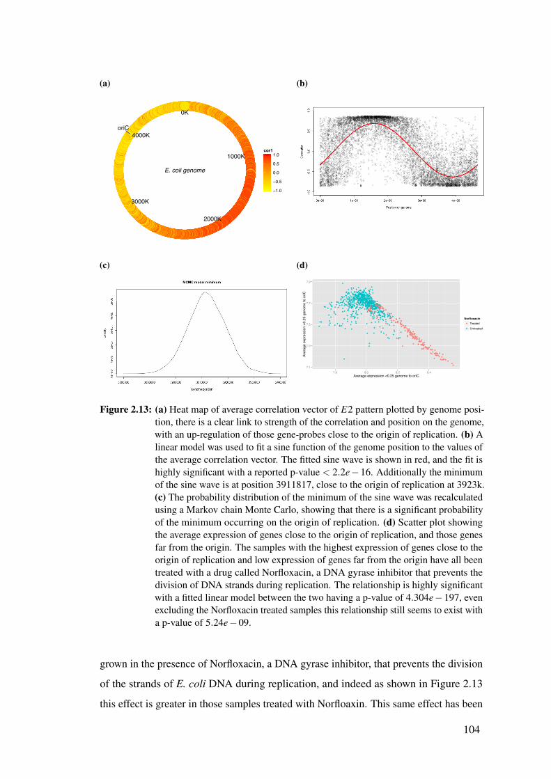
(a)
oriC
0K
1000K
2000K
3000K
4000K
E. coli genome
−1.0
−0.5
0.0
0.5
1.0cor1
(b)
(c) (d)
●●
●●●●●
●
●
●
●
●
●●
●●●
●
●●●
●
●
●
●
●
●
●
●
●
●●●
●●●●●●●●
●
●
●
●●
●●
●●●●●
●
●
●
●
●●
●
●●
●●
●
●●
●
●●●●
●●●
●
●●
●●
●
●
●
●
●●
●●●●
●
●●●●
●
●●
●●●●
●●
●●
●●
●●
●
●●
●●
●
●●
●
●
●
●●●●
●
●
●●
●●●
●
●●
●●
●●
●
●
●
●
●●
●
●
●●●●
●●
●
●
●
●
●●
●
●
●
●●
●
●●
●
●
●
●●●●●●
●
●
●
●
●
●
●
●
●
●
●
●
●
●
●
●
●●●
●
●●
●●
●
●
●
●●●
●●
●
●
●
●●
●
●
●
●
●●
●
●
●●
●
●
●
●
●●
●
●●●
●
●
●
●
●
●●●●
●
●
●
●●●●
●
●●●
●
●
●
●●●
●
●
●
●
●●●●
●●●
●●●●●●●●
●
●
●
●
●●
●●
●●
●●
●●●●●
●
●
●
●
●
●
●
●
●
●
●
●
●
●
●
●
●
●
●
●●
●
●
●
●●
●
●
●●
●
●
●
●
●●
●
●●
●
●●
●
●
●
●
●●●
●
●●●
●
●
●
●
●
●
●
●●
●●
●
●
●
●
●
●
●
●
●
●
●
●●
●●
●
●
●
●
●
●
●
●
●●
●
●●
●
●
●●
●●
●
●
●
●
●●
●
●●
●
●●●●
●
●
●
●
●
●
●
●
●
●●●
●
●
●
●
●
●
●
●
●
●●
●
●
●
●
●
●
●
●
●
●
●
●●
●●
●
●
●●
●
●
●
●
●
●
●
●●
●●
●
●
●
●
●
●●●
●
●●
●
●
●●
●
●●
●
●●●●●
●
●
●
●
●
●
●
●
●●●
●
●
●
●
●
●●●
●
●
●
●
●
●
●●
●
●
●
●
●
●
●
●
●
●
●●●
●
●
●
●●
●
●
●
●
●
●●
●
●
●
●
●
●●
●●●●
●
●
●●
●●
●●
●●●
●●
●
●
●
●
●
●
●
●
●
●
●
●
●
●●
●●●
●
●
●
●
●●●
●
●
●●
●
●
●
●
●●
●●
●
●
●
●
●●●
●
●
●
●
●●●
●●●
●
●●●
●
●
●
●●●●
●
●
●
●
●
●
●
●
●●
●●●●
●
●
●●
●
●
●
●
●●
●●
●●
●
●
●
●
●
●
●
●
●
●
●
●
●●
●
●
●
●
●
●
●
●
●
●●
●
●●●
●
●
●
●
●
●
●●
●●●
●
●
●
●
●
●
●
●
●●
●
●
●
●
●
●
●
●●
●
●
●●
●●
●
●
●
●
●
●
●
●
●
●
●
●
●
●●
●
●
●
●
●●●
●
●
●●
●●
●
●
●
●
●●
●
●
●
●●
●
●
●
●
●●●
●
●●
●
●●
●
●●●
●
●
●
●
●
●
●
●
●
●
●
●
●●
●
●
●
●
●
●
●
●●
●
●
●
●
●
●
●
●●
●
●
●●●
●
●
●●
●
●
●●●
●
●
●
●
●
●
●
●
●
●
●●
●
●
●
●
●
●
●
●
●
●
●
●
●
●
●
●
●
●
●
●
●
●
●
●
●
●
●
●●
●
●
●
●
●
●●
●
●
●
●
●●
●
●
●
●
●●
●
●
●●
●
●
●
●
●●
●●
●
●
●
●
●
●
●
●
●
●●●
●●
●
7.1
7.3
7.5
7.7
7.9
7.8 8.0 8.2 8.4Average expression <0.25 genome to oriC
Aver
age
expr
essi
on >
0.25
gen
ome
to o
riC
Norfloxacin●
●
TreatedUntreated
Figure 2.13: (a) Heat map of average correlation vector of E2 pattern plotted by genome posi-tion, there is a clear link to strength of the correlation and position on the genome,with an up-regulation of those gene-probes close to the origin of replication. (b) Alinear model was used to fit a sine function of the genome position to the values ofthe average correlation vector. The fitted sine wave is shown in red, and the fit ishighly significant with a reported p-value < 2.2e�16. Additionally the minimumof the sine wave is at position 3911817, close to the origin of replication at 3923k.(c) The probability distribution of the minimum of the sine wave was recalculatedusing a Markov chain Monte Carlo, showing that there is a significant probabilityof the minimum occurring on the origin of replication. (d) Scatter plot showingthe average expression of genes close to the origin of replication, and those genesfar from the origin. The samples with the highest expression of genes close to theorigin of replication and low expression of genes far from the origin have all beentreated with a drug called Norfloxacin, a DNA gyrase inhibitor that prevents thedivision of DNA strands during replication. The relationship is highly significantwith a fitted linear model between the two having a p-value of 4.304e�197, evenexcluding the Norfloxacin treated samples this relationship still seems to exist witha p-value of 5.24e�09.
grown in the presence of Norfloxacin, a DNA gyrase inhibitor, that prevents the division
of the strands of E. coli DNA during replication, and indeed as shown in Figure 2.13
this effect is greater in those samples treated with Norfloaxin. This same effect has been
104

previously shown to exist in Streptococcus pneumoniae by Slager et al. (2014) who
showed that upon treatments with antibiotics that stall bacterial DNA replication, there
is a up-regulation of genes close to the origin of replication. Interestingly Streptococcus
pneumoniae has evolved so that genes close to the origin of replication when up-regulated
trigger bacterial competence in response to antibiotics.
The biclustering algorithm has therefore found 3 distinct biclusters within the E.
coli data, these biclusters represent complex regulatory patterns resulting from either
transcriptional programs or response to environmental conditions.
2.4.4 Analysis of random probe sets
It can be noticed from Figures 2.12(b) and 2.13(d), that the biclusters identified both
are represented by the identification of two probe sets which are anti-correlated to each
other. That is there are two probe sets, in which when one is up-regulated, the other is
down-regulated.
It can however be observed that this is not the general case. Upon randomly dividing
the measured probes into two sets, it is relatively easy to take an average of these two
probe sets and plot in a similar manner the samples as was done in Figures 2.12(b) and
2.13(d). This can in fact be done computationally 1000 times, and Figure 2.14 shows an
example of this being done along with the distribution of the correlation between the
two probe sets.
As can be seen from 1000 randomly generated pairs of probe sets all had a strong
positive correlation and none had a correlation less than 0.86. Two things need to be
explained, why random probe sets have such a strong positive correlation and why the
probe sets found from the biclustering analysis have such strongly negative correlations?
To explain the strong positive correlation, these probe sets being random, it would
be highly unlikely if they were to share a functional role. It is possible that these average
values therefore only reflect the average value of all probes being measured of which
there is some variation across the samples. The fact that this variation exists in this
dataset, could potentially highlight an issue with normalisation as on average some
samples have a higher average gene expression value than others. These differences
however are generally small, and natural variation may indeed be expected to exist in
the average gene expression values between different biological samples.
105

(a)
(b)
Figure 2.14: (a) A scatter plot showing the average of two random probe sets for all the samplesin the E. coli dataset. The two random probe sets were created one of size 3720 andthe other of size 3719, to cover all of the 7439 probes measured. (b) A frequencyhistogram plot of the correlation between two randomly generated probe setscreated in the manner of (a) repeated 999 more times.
The biclustering analysis however has not picked out random probes but biologically
relevant patterns. In transcriptional programs, genes are only up or down-regulated in
relation to other non-changing genes, comparing the two up and down-regulated gene
sets will therefore always result in a strong negative correlation and such a negative
106

correlation is the hallmark of a non-random regulation effect.
2.5 ConclusionThe aim of this chapter was twofold, firstly to introduce a novel bioinformatic technique,
MCbiclust, that can be used to investigate mitochondrial biogenesis in disease, and
secondly to demonstrate its validity and usefulness for this role.
The first task of this was accomplished by the development of a novel biclustering
algorithm specifically designed to study mitochondrial biogenesis. The development in
detail is described in Section 2.2. Additionally information of the implementation of
this algorithm and associated methods in R will be given in Appendix A.
Once the method was fully introduced the next major task was to demonstrate its
validity in tackling the problem set of studying mitochondrial biogenesis. To do this
it had to be shown to be superior to other existing biclustering methods that were not
designed to examine such large regulation patterns exclusively.
For this aim a synthetic dataset was created that reproduced the size of a bicluster
representing mitochondrial biogenesis as well as the scale of the large datasets that are
available to study. On achieving this by various measures such as the F1 score and
examining ROC plots, MCbiclust was found to be superior to alternative methods even
though it only found 6 of the 8 synthetic biclusters.
Finally MCbiclust was demonstrated on a real dataset, containing bacterial E. coli
samples. Due to mitochondria’s bacterial origin, E. coli can be thought of as a similar
transcriptional complexity to an investigation of mitochondrial biogenesis. The method
was extremely successful in identifying biological relevant patterns, including some
involving very novel effects such as a compound causing inhibition of division of DNA
during replication leading to an up-regulation of genes close to the origin of replication.
There are perhaps some weaknesses in the current method, this mainly involves
there being one or more biclusters that dominate the results such that any other biclusters
are not found. This appears to be the case for the two synthetic biclusters that were
not identified, and was apparent in the E. coli analysis where the bicluster involving
intergenic regions was only identified due to one outlier sample, where the signal was
much stronger. It may be possible in future to build an adapted version of the method
described here which can identify these weak signal patterns.
107

Despite this, overall the method developed is a great improvement over existing
techniques and seems absolutely suitable for the investigation of mitochondrial biogen-
esis in disease. While potentially it will not be able to find all the different modes of
regulation for mitochondrial biogenesis, it has the potential to identify the major modes
of regulation present in the data. This will be the focus of the next chapter, specifically
focusing on the regulation of mitochondrial biogenesis in hypertrophic cardiomyopathy
and different cancer cell lines.
108

Chapter 3
Bioinformatic analysis of
mitochondrial biogenesis in disease
3.1 IntroductionFollowing the establishment in Chapter 2 of the Massively Correlating Biclustering
(MCbiclust) as a method for finding large scale biclusters in transcriptomic data, it is
time to attempt to use these methods for their intended aim of studying alterations of
mitochondrial biogenesis in disease.
The focus of this chapter will be on two pathologies: cancer and heart disease.
These two diseases and their relationship to mitochondrial function were previously
discussed in Section 1.4.1 on page 52 for cancer and Section 1.4.2 on page 56 for heart
disease. Both cancer and heart disease are conditions that describe a large number of
clinically distinct disorders; in both these cases MCbiclust will only be run on a single
dataset. This is so that the utility of MCbiclust in investigating mitochondrial function
can be demonstrated, as well as its suitability for a more extensive investigation of the
variety of mitochondrial biogenesis regulation in these disorders.
It has been previously shown that MCbiclust is capable of finding these patterns,
but precise knowledge of its statistical power to do so is hard to define. Say, for example
if a bicluster contains 50% of the known mitochondrial genes, roughly 500, and includes
10% of all samples, so 100 samples in a dataset containing 1000 in total; then the total
number of possible biclusters matching this is roughly 1.7⇥10439. How many of these
possible mitochondrial related biclusters represent a true biologically significant pattern?
It is not computationally possible to check them all. While MCbiclust certainly finds
109

relevant mitochondrial related biclusters it is not possible to say all relevants biclusters
have been found without checking all possibilities.
According to this purpose, for heart disease, MCbiclust will be applied to a dataset
concerning hypertrophic cardiomyopathy from Hebl et al. (2012). While for cancer
MCbiclust will be applied to a dataset from the Cancer Cell Line Encyclopeadia (Bar-
retina et al. 2012).
3.1.1 Hypertrophic Cardiomyopathy (HCM)
Hypertrophic cardiomyopathy (HCM) is a genetic cardiac disease, characterised by a
thickening of the myocardium, the muscle tissue of the heart.
HCM is more precisely characterised by a disordered arrangement of myocytes and
asymmetric patterns of left ventricle wall thickening (Maron 2015). Pathologically the
course of the disease varies considerably, and Figure 3.1 shows the possible outcomes
of which a large percentage of patients have a benign form of HCM and will not require
treatment. It is important to note that this benign form is distinct from the condition
known as athletic heart syndrome, which is a non-pathological condition in which the
heart is enlarged from regular exercise.
Overall HCM can be divided into two main subtypes, obstructive and non-
obstructive with the obstructive patients having a significantly worse prognosis if un-
treated. Obstructive here refers to a blocking of the left ventricle outflow tract caused by
wall thickening. This is a serious condition that can lead to progressive heart failure or a
stroke; it is also easily treated by surgery with a myectomy that removes a small amount
of the muscle to increase the left ventricle outflow. Patients treated with a myectomy in
a sense are fully recovered with long-term survival post operation being equivalent to
the general population.
Besides surgery, the likelihood of heart failure for both obstructive and non-
obstructive cases can be reduced through treatment by beta-blockers (Maron 2015).
In a few extreme cases neither drug treatment or surgery avoid advanced heart failure
but in even these cases, patients can receive a heart transplant and expect a full recovery.
HCM is perhaps most widely known for the minority of cases in which the patients
remain asymptomatic until undergoing sudden cardiac death, and this is one of the
leading causes of sudden death in the young and has been notable in the media for being
110

Figure 3.1: Possible clinical outcomes of HCM. Figure is taken from (Maron 2015), mostcases of HCM are benign, however for pathological outcomes they can be treatedby various means such as septal myectomy surgery, the use of an implantablecardioverter-defibrillator (ICD), drug treatment or in extreme cases a heart transplant.AF in the diagram refers to atrial fibrillation.
the cause of death of otherwise healthy young athletes (Maron 2003). Even in these
cases however if the risk of sudden death can be identified a treatment option is possible
with the use of an implantable cardioverter-defibrillator (ICD) which can detect and treat
potentially fatal arrhythmias in HCM patients (Maron 2015).
Therefore, there are possible modes of treatment for all pathological outcomes of
HCM, though in the case of preventing sudden death it is essential to determine those
patients at high risk. Due to the large rate of progress in treating HCM it has been
recently declared to be a contemporary treatable disease (Maron 2012).
It has been previously estimated that HCM effects 1 : 500 of the population (Maron
et al. 1995) though recently it has been thought that the population effected is higher and
this has recently been revised upward to 1 : 200 (Semsarian et al. 2015). This has partly
come about due to the greater use of genetic screenings, and an appreciation that there
are individuals who have a mutation causing HCM who are at risk of but not developed
the phenotypic symptoms.
HCM is best known for occurring from mutations in sarcomere proteins, proteins
111
that form the basic unit of striated muscle tissue. With more than 1000 individual
mutations causing HCM identified in 11 sarcomere protein genes (Maron et al. 2012).
In addition to this sarcomere connection there are possible reasons to suggest that the
mitochondria may play a role in the development of HCM. This is mainly due to the
apparent occurrence of HCM in various mitochondrial diseases.
Smits et al. (2011) reported a case where a mutation in the mitochondrial ribosome
gene MRPS22, caused brain anomalies as well as hypertrophic cardiomyopathy. More
generally Holmgren et al. (2003) found that out of 101 patients with mitochondrial
diseases 17 were discovered to have HCM of the non-obstructive type, suggesting that on
a whole patients with mitochondrial defects are more likely to have HCM. Additionally
Wang et al. (2007) noted that patients with polymorphisms of mitochondrial master
regulator peroxisome proliferator-activated receptor gamma coactivator 1-a (PGC-1a)
are more likely to develop HCM.
Despite this known association with mitochondrial defects, little is known about
the exact role mitochondria plays in HCM. For these reasons HCM is a good case
model for studying the role of mitochondrial biogenesis using the novel biclustering
technique developed in Chapter 2. Greater understanding of the role mitochondria plays
in HCM has the potential to lead to better determination of a patients risk of sudden
death and aid clinical decisions as well as understanding what differentiates the benign
and pathological versions of the disease.
3.1.2 Cancer cell lines
Cancer cell lines are derived from tumours taken from patients; these cells have then
gone through a process called immortalisation such that they can be grown continuously
in the lab. The first cancer cell line to be produced were HeLa cells that were taken from
a woman called Henrietta Lacks who died from cervical cancer in 1951 (Skloot 2010).
Since then HeLa and other cancer cell lines have been widely cultured and used by
scientists as an easily available model to study cancer and molecular cellular function.
Cancer cell lines are sometimes criticised for not being representative of the tumour
they derive from (Masters 2000). In some senses this is true since they are grown in
vitro in an environment very dissimilar to a real tumour, and additionally the cancer cell
line has had to undergo immortalisation involving selective pressure for certain genetic
112

changes to continuously grow in lab conditions.
Despite this they are still valuable tools; research into the gene expression profiles
of cancer cell lines reveal a distinct correspondence to their tissue of origin (Ross et al.
2000), this suggests the cancer cell lines can be used as a relevant model for studying
cancer.
What is more, studies such as Barretina et al. (2012) use cancer cell lines as a
pre-clinical model to test for drug sensitivity. Such research therefore has the potential
to identify important biomarkers in cancer, such as distinct gene expression patterns or
copynumber changes, present in both cancer cell lines and patient tumours. For this
reason cancer cell lines are an ideal model to use to investigate the role alterations in
mitochondrial biogenesis plays in cancer.
3.2 Bioinformatic analysis of mitochondrial biogenesis
in hypertrophic cardiomyopathy
3.2.1 The data
The dataset from Hebl et al. (2012) contains 107 RNA-Seq samples from patients
with HCM and 39 control samples. The disease tissue RNA was extracted from tissue
collected following septal myectomy, a surgery treatment for HCM that removes a
portion of the septum obstructing blood flow, while the control samples were collected
from healthy donor hearts. As all the patients representing HCM in this dataset have
undergone septal myectomy, the dataset only represents patients with one of the possible
pathological outcomes of the disease. This leads to some bias within the data and it is
not possible to study how differences in mitochondrial biogenesis cause some cases to
be benign and others not.
For both the HCM samples and controls 37,846 genes were measured using the
Illumina HumanHT-12 v3 Expression BeadChip. Unfortunately the publicly available
dataset (Gene Expression Omnibus accession number GSE36961) contains no additional
clinical data of interest.
The original analysis undertaken by Hebl et al. (2012) examined the differentially
expressed genes between the HCM tissue and the controls, and not whether there are
any distinct subtypes of HCM samples with a different expression profile. For this
113

reason, this dataset is ideal to search for biclusters that find distinct modes of regulation
occurring in only a subset of the samples.
The novel biclustering method MCbiclust described in Chapter 2 therefore was
applied to the HCM data. Two sets of initial runs were done, on both the control and
disease samples together. The first was a set of 1000 runs aiming to find biclusters
involving the mitochondrial genes described by MitoCarta (Pagliarini et al. 2008). The
second was a set of 1000 runs where each run used a different random gene set containing
1000 genes.
The rationale behind the runs with the random gene sets is to find general biclusters
that affect a large proportion of the transcriptome. These biclusters may be the same as
the ones found with the MitoCarta gene set, indicating significant mitochondrial change
also coincide with large scale changes affecting non-mitochondrial genes.
3.2.2 Silhouette plots and ranking the samples
The first step in the analysis for both the MitoCarta and random gene set runs is to
identify how many distinct biclusters are found, and this is done using a silhouette plot
analysis. For the MitoCarta gene runs, examining the silhouette plot seen in Figure 3.2
(a - b) shows that the optimum number of clusters is 1, with the highest silhouette width
occurring when all 1000 correlation vectors are clustered together compared against the
randomly generated correlation vector. This bicluster was named Mito.1. Similarly for
the set of random gene runs, the result from the silhouette analysis is that the optimum
number of clusters is 1, this can be seen in Figure 3.2 (c - d). This bicluster was named
Random.1.
For each of the runs, one of the sample seeds was chosen such that the correlation
score was maximum for the top 1000 genes in the average correlation vector from
the clustered groups. Using this sample seed and the top 1000 genes in the average
correlation vector, all the samples could be ranked by how well they matched the
correlation pattern.
Following the ranking of the samples, the correlation pattern can be summarised
using principal component analysis, and have the strength of the correlation in each
sample numerically quantified by the value for the first principal component. Figure 3.3
shows the first principle component plotted against the ranked samples for both biclusters
114

(a)
5 10 15 20
0.4
0.5
0.6
0.7
0.8
Number of clusters
Mea
n si
lhoe
tte w
idth
(b)
Silhouette width si
0.0 0.2 0.4 0.6 0.8 1.0
Average silhouette width : 0.85
n = 1001 2 clusters Cj
j : nj | avei∈Cj si
1 : 1000 | 0.85
2 : 1 | 0.00
(c)
5 10 15 20
0.2
0.4
0.6
0.8
Number of clusters
Mea
n si
lhoe
tte w
idth
(d)
Silhouette width si
0.0 0.2 0.4 0.6 0.8 1.0
Average silhouette width : 0.93
n = 1001 2 clusters Cj
j : nj | avei∈Cj si
1 : 1000 | 0.93
2 : 1 | 0.00
Figure 3.2: Silhouette analysis of two sets of runs in the HCM data. Figures (a) and (b) showthe mean silhouette width for different numbers of clusters and the silhouette plotfor the correlation vectors from the run on the MitoCarta genes while Figures (c)and (d) show the same but for the runs from the random gene sets. In both cases thedata was best grouped into a single cluster when ignoring the randomly generatedcorrelation vector inputted into the analysis for comparison. A single cluster isnarrowly the optimum way of clustering for the MitoCarta runs while for the randomgene set runs it is by far the best.
found.
Figure 3.3 clearly shows two distinct ‘forks’ representing the biclusters. The Mito.1
fork from the MitoCarta gene set is especially of interest as the upper fork is made
up entirely of control samples. It can be checked by examining a plot of the average
expression value of the mitochondrial genes (shown in Figure 3.4) that this signifies that
the pattern represents a down-regulation of the mitochondria in these control samples
compared to the rest of the samples in the dataset. Conversely it can be viewed that in
the disease samples there is a up-regulation of mitochondrial genes compared to this
healthy control subset. This is interesting as it represents a mode of regulation involving
the mitochondria that only occurs in healthy samples and not disease.
115

(a)
−20
−10
0
10
20
30
0 50 100 150order
PC1
factor(Status)ControlSample
(b)
−20
−10
0
10
0 50 100 150order
PC1
factor(Status)ControlSample
Figure 3.3: PC1 plots of two sets of runs in the HCM data. Figure (a) shows the PC1 plottedagainst the ranked samples from the bicluster found with the mitochondrial geneset (Mito.1 bicluster). This clearly separates control and disease samples across theranking, though there is one control sample grouped with the disease samples at thebeginning of the ranking, possibly indicating an unknown mitochondrial defect ineither that control sample or the control samples making up the upper fork. The PC1plot against the ranked samples from the bicluster found with the random gene setsis given in Figure (b) (Random.1 bicluster). This shows a difference that seems toaffect both control and disease samples, with the effect being notably stronger in asingle disease outlier sample.
Another notable point from this is that the biclustering algorithm found no biclusters
representing different types of regulation of mitochondria in any HCM samples. For
this reason it was thought important to have one more set of runs with the mitochondrial
genes but no control samples.
This was done and a silhouette analysis (Figure 3.5) was found to identify 3 distinct
biclusters, named Mitonc.1, Mitonc.2 and Mitonc.3. As done on the other two biclusters
previously found, a sample ranking was made for these 3 new biclusters as well as a
principal component analysis to summarise the correlation pattern found with the first
principal component. In the ranking of the samples, control samples were allowed back
in, since their absence from the sample seed was enough to ensure that distinct biclusters
showing mitochondrial differences between disease samples were found. PC1 plots can
be seen in Figure 3.6.
3.2.3 Comparing the biclustersOverall from the three sets of runs, 5 biclusters were identified. These can be directly
compared with each other by three means:
1. The ranking order of the samples.
116

(a)
8.6
8.7
8.8
8.9
0 50 100 150order
Aver
age
Mito
chon
dria
l gen
e ex
pres
sion
factor(Status)ControlSample
Figure 3.4: Average mitochondrial expression plot of Mito.1 pattern reveals that mitochondriaexpression is downregulated in a subset of the control samples compared to the restof the samples in the dataset.
(a)
5 10 15 20
0.55
0.65
0.75
Number of clusters
Mea
n si
lhoe
tte w
idth
(b)
Silhouette width si
−0.2 0.0 0.2 0.4 0.6 0.8 1.0
Average silhouette width : 0.83
n = 1001 4 clusters Cj
j : nj | avei∈Cj si
1 : 297 | 0.90
2 : 577 | 0.82
3 : 126 | 0.714 : 1 | 0.00
Figure 3.5: (a) and (b) show the silhouette analysis set of runs in the HCM data on mitochondrialgenes without the controls revealing three distinct biclusters. These biclusters werenot found previously when the controls were included, indicating that the overallstrength of the correlations involved must be weaker.
2. The individual values of the correlation vectors.
3. Gene set enrichment of the correlation vectors.
117

(a) Mitonc.1
10
20
30
0 50 100 150order
PC1
factor(Status)ControlSample
(b) Mitonc.2
−10
0
10
20
0 50 100 150order
PC1
factor(Status)ControlSample
(c) Mitonc.3
−20
−10
0
0 50 100 150order
PC1
factor(Status)ControlSample
Figure 3.6: PC1 plots of biclusters from set of runs in the HCM data on the mitochondrial geneswithout controls.
Since there is limited clinical information for the samples besides whether they are
a control or not, all comparisons must be done using the correlation vectors themselves.
The simplest way to do this is to numerically compare the values in the correlation
vectors themselves. Two correlation vectors describing a similar pattern will be strongly
correlated. Therefore if any of the 5 distinct correlation vectors identified are strongly
correlated to each other, it is enough to say that they are describing the same pattern.
Figure 3.7 shows all 5 bicluster correlation vectors compared by using scatter
plots, examining mitochondrial and non-mitochondrial genes separately. From this it is
apparent the bicluster identified from the random gene sets, Random.1, is highly similar
to one of the biclusters identified from the MitoCarta gene set run with no controls,
Mitonc.1. This therefore shows that there are only 4 distinct biclusters found from the 3
sets of runs that need to be examined in detail.
118

Figure 3.7: Comparison plot of the correlation vectors from the 5 biclusters found in the HCMdata. Each distinct bicluster that has been identified has an average correlationvector associated with it, that describes how each gene measured correlates withthe bicluster. These different correlation vectors can compared against each otherin a scatter plot. If there is a strong correlation between the different correlationvectors as can be seen between bicluster Random.1 and Mitonc.1this indicates thatthe two biclusters are highly similar. In this figure the lower diagonal scatter plotsin blue represent the non-mitochondrial genes, while the upper diagonal scatterplots in red represent the mitochondrial genes. The plots on the diagonal show themitochondrial and non-mitochondrial histogram for each bicluster. Two correlationvectors can be distinct, yet contain large modules of genes that are regulated in thesame way, this can be seen between the Mito.1 and Mitonc.3 biclusters that containa high density of mitochondrial genes regulated similarly in both biclusters.
It is also possible that while two correlation vectors are distinct, they share gene
modules that are regulated in similar ways. For instance, on closer examination of
Figure 3.7 between Mito.1 and Mitonc.3 there appears to be a small module of mito-
119

chondrial genes that are similarly regulated despite the majority of the mitochondrial
genes not being similarly regulated between the different biclusters.
This gene module can be examined, as can be seen in Figure 3.8, the genes in the
identified modules were selected as those that have a correlation vector greater than 0.75
in both the Mito.1 and Mitonc.3 biclusters.
168 of the total 900 mitochondrial genes measured in the HCM had a correlation
vector greater that 0.75 for the Mitonc.3 pattern, while 352 genes had a correlation
vector greater than 0.75 for the Mito.1 pattern. The intersection of these 2 groups was 86
genes, the number of genes in this intersection can be modelled using the hypergeometric
distribution, considering genes belonging to both gene sets a success.
In general with a gene set of size N with two subsets selected of size a and b and
b > a the probability of the size of the intersection being x will follow a hypergeometric
distribution:
P(x) =
�N�ab�x
��ax�
�Nb� (3.1)
In this case N = 900, a = 168 and b = 352. Using this the mean expected size of
the intersection can be calculated as b aN = 352168
900 ⇡ 65.7, and P(X � 86) = 0.00029.
Thus the size of this gene module is larger than expected if they were selected randomly,
and indicates that there are genes in the module that are co-regulated. While this is
not a huge module of co-regulated genes it is statistically significant and demonstrates
the ability of this method to find these modules of co-regulated genes between distinct
biclusters.
The group of genes in the module are given in Table 3.1 along with the correlation
vector values in the relevant biclusters, the gene list includes genes that very well may
be coregulated such as members of the electron transport chain (ETC) notably for ATP
synthase, Complex I, the fatty acid beta oxidation pathway and genes encoding the
mitochondrial ribosome.
The discovery of these co-regulated mitochondrial modules give some indication
to how the regulation of mitochondrial biogenesis functions. Presumably these modules
exist due to some effect of members of the transcription factor network controlling mito-
chondrial biogenesis. Importantly the existence of these differences in the mitochondrial
120

Mito.1 Mitonc.3ABHD11 0.94 0.77
ACAA2 0.86 0.85ACADM 0.94 0.90
ACADSB 0.95 0.76ACAT1 0.97 0.88ACN9 0.85 0.88
ACOT2 0.92 0.84AFG3L2 0.85 0.84
AIFM1 0.97 0.87AKAP1 0.89 0.93
ALDH5A1 0.98 0.94AS3MT 0.91 0.92ATAD1 0.88 0.88
ATP5F1 0.93 0.96ATP5G3 0.94 0.79ATPAF1 0.96 0.84
AUH 0.93 0.92BCKDHB 0.94 0.91
BDH1 0.93 0.76CHCHD4 0.94 0.88CHCHD7 0.96 0.86
COQ3 0.97 0.88DCI 0.80 0.80
DHTKD1 0.79 0.90DLAT 0.89 0.86DLD 0.84 0.97
EARS2 0.82 0.83EHHADH 0.96 0.83
GFM2 0.93 0.88GPAM 0.90 0.79
GTPBP8 0.94 0.91HADH 0.98 0.87
HIGD1A 0.80 0.91HRSP12 0.85 0.93HSDL2 0.94 0.83IARS2 0.87 0.86
IMMP2L 0.83 0.89IMMT 0.81 0.88LDHB 0.79 0.96
LIAS 0.95 0.85MAOB 0.98 0.95
MCCC2 0.95 0.83MCEE 0.95 0.86
Mito.1 Mitonc.3ME2 0.84 0.81
MIPEP 0.91 0.76MLYCD 0.88 0.80MOSC2 0.95 0.85
MRPL16 0.80 0.84MRPL39 0.79 0.92MRPS10 0.77 0.80
MRPS7 0.87 0.84MRRF 0.90 0.76MTX2 0.88 0.80MUT 0.92 0.78
NDUFA10 0.90 0.88NDUFAF1 0.77 0.90
NDUFB3 0.90 0.82NDUFB5 0.86 0.85NDUFB6 0.84 0.78NDUFS2 0.85 0.90
NNT 0.98 0.94OMA1 0.98 0.90
OSGEPL1 0.96 0.93OXCT1 0.93 0.81PACRG 0.88 0.88PCBD2 0.95 0.79
PCCA 0.91 0.86PECI 0.87 0.88
PET112L 0.96 0.87PHYH 0.92 0.86PINK1 0.89 0.80
PMPCB 0.91 0.81PRDX2 0.90 0.83PRDX3 0.96 0.87PTCD2 0.98 0.80
PTGES2 0.86 0.77QDPR 0.97 0.90
SARS2 0.76 0.78SCO1 0.91 0.79SDSL 0.94 0.80SIRT5 0.97 0.89
SLC25A20 0.91 0.86SUCLA2 0.97 0.94TATDN3 0.97 0.92
TOMM20 0.83 0.82UQCRC2 0.85 0.96
Table 3.1: Mitochondrial co-regulated gene module identified in two different biclusters
transcriptional program between different HCM samples also confirms that there are
subtypes with different mitochondrial regulation.
121

ACOT2
PRDX2
MRPS
7MRRF
ACAD
SBPT
CD2
EHHAD
HIMMP2L
ACN9
LIAS
QDPR
MCEE
PTGES
2MCCC2
NDUFB
6TO
MM20
MIPEP
BDH1
DCI
AIFM
1MLYCD
CHCHD4
ABHD11
SIRT
5MAO
BMRPS
10NDUFB
3SD
SLSLC25A20
BCKD
HB
AUH
GFM
2OXC
T1NDUFAF1
EARS2
PACRG
PINK1
CHCHD7
MUT
NDUFA10
IARS2
NDUFS
2PE
T112L
SARS2
PCCA
MOSC
2DHTK
D1
AFG3L2
MRPL16
NDUFB
5OSG
EPL1
TATD
N3
PRDX3
ACAT1
ATP5F1
COQ3
HSD
L2HAD
HPC
BD2
SCO1
ATP5G3
DLAT
HIGD1A
HRSP
12AC
ADM
IMMT
UQCRC2
MRPL39
ACAA
2SU
CLA2
ATPAF1
PMPC
BOMA1
ATAD
1NNT
ME2
PHYH
LDHB
ALDH5A1
MTX
2GPAM
PECI
GTP
BP8
DLD
AKAP
1AS
3MT
Mitonc.2
Random.1
Mitonc.1
Mitonc.3
Mito.1
−0.5 0 0.5Value
060
Color Keyand Histogram
Count
Figure 3.8: Heat map showing a module of similarly regulated mitochondrial genes in thecorrelation vector values. Mitochondrial genes that had correlation values greaterthan 0.75 in both the Mito.1 and Mitonc.3 biclusters were selected, this revealed alarge subgroup that has many terms related to the ETC.
3.2.3.1 Gene set enrichment
The final method of comparing the different biclusters is by using gene set enrichment.
By applying this on the correlation vectors this will find not only the significant mi-
tochondrial terms, but all the significant non-mitochondrial terms as well. Although
our primary interest is the regulation of mitochondrial biogenesis in disease models,
mitochondria have to react to changes in the cellular environment. The significant
non-mitochondrial terms therefore tell us of what wider cellular transcriptional program
the change in mitochondrial regulation is related to.
There are 998 significant gene ontology (GO) terms found from the Mito.1 pattern.
A table of the top 200 terms by significance is given in Table B.4. The vast majority of
significant terms have a negative average correlation vector value, the exceptions are
terms related to the mitochondria that have positive average correlation vector values.
This implies that when the healthy samples have a large number of downregulated
mitochondrial genes compared to the disease samples, as is seen in Figure 3.4, all
these other terms are upregulated. These up-regulated terms include strongly those
related to the immune system, ribosome biogenesis and cell proliferation. Since only the
healthy control samples had their mitochondria down-regulated during this up-regulation
122

of cellular proliferation, while the disease samples conversely had their mitochondria
up-regulated during down-regulation of cellular proliferation, it is tempting to form a
hypothesis that the switch in this regulation could lead to HCM.
The other biclusters seem to describe either different regulation between different
HCM samples or a type of regulation that exists in both HCM and control samples.
For the Random.1 and Mitonc.1 biclusters the significant terms are similar to
eachother, with 200 of the 213 significant terms of Mitonc.1 also being significant for
Random.1, and do not seem to be much related to mitochondrial function, with only
the 13 terms only significant in Mitonc.1 being related to mitochondrial function. It is
hard to see a general functional role for all these significant terms, 482 for the Random.1
pattern and 213 for the mitonc.1 pattern, with many generic high-level terms describing
broad biological processes such as binding being significant. A full table of these
significant terms is given in Table B.5 and B.6.
The Mitonc.2 and Mitonc.3 bicluster were identified as being potentially related
to mitochondrial function but not involving the control samples. The Mitonc.3 sig-
nificant terms seems to be exclusively related to the mitochondria with very few non-
mitochondrial terms being highly significant. There are relatively few Mitonc.2 signif-
icant terms and these also are fairly general and do not give much of an indication of
what the pattern in Mitonc.2 represents. The significant terms for Mitonc.2 and Mitonc.3
are given in Tables B.7 and B.8 respectively.
While not a lot is known about these biclusters due to the absence of additional
clinical data, all identified biclusters represent a real biological effect. Strikingly one of
these biclusters separated the control and disease samples, and seems to suggest a mode
of regulation not existing in either the control or disease samples. With the additional
discovery of modules of co-regulated mitochondrial genes, this demonstrates that this
technique can be used to study the role of the regulation of mitochondrial biogenesis in
disease.
123

3.3 Bioinformatic analysis of mitochondrial biogenesis
in cancer cell lines
3.3.1 The data
The Cancer Cell Line Encyclopedia (CCLE) (Barretina et al. 2012) is a dataset created
by the Broad Institute to provide detailed characterisations of a wide range of human
cancer cell lines on the gene expression level. In addition to this, the data includes the
chromosomal copy number across 947 human cancer cell lines, and has the pharmaco-
logical profiles for 24 anticancer drugs across 479 cancer cell lines. Within this dataset,
due to the heterogeneous nature of cancer, it is expected that there is large variations in
the modes of regulation. This is especially true as the total collection of cell lines come
from 36 different tumour types (Barretina et al. 2012).
For the data generated by Barretina et al. (2012), the gene expression levels were
measured from messenger RNA using Affymetrix U133 plus 2.0 arrays, while DNA
copy number was measured using high-density single nucleotide polymorphism arrays.
To measure the pharmacological profile of the cell lines, a 8-point dose-response curve
for 24 anticancer compounds was generated for 479 of the cell lines.
By using the biclustering algorithm different regulations of mitochondrial biogene-
sis as well as other pathways can be investigated in much the same way as was done for
hypertrophic cardiomyopathy. Any biclusters found can then additionally be understood
using the copy number and the pharmacological data.
Like the HCM dataset, two sets of runs were done, one using the MitoCarta genes
(Pagliarini et al. 2008) and the other using random probe sets. Both included 1000 runs
of the biclustering algorithm.
3.3.2 Silhouette plots and comparison
Once both of the sets of runs were completed, silhouette width analysis was used to
determine the number of distinct biclusters. For the MitoCarta set, it was shown that
there was only one distinct bicluster, as can be seen in Figure 3.9(a - b). For the random
probe set, the silhouette results showed that there were two distinct biclusters, this can
be seen in Figure 3.9(c - d) with three biclusters being identified from the silhouette
analysis, and no reason to include an additional set of runs as was required for the
124

analysis of the HCM dataset, the next step is to compare all the biclusters found to judge
their similarity. This is done in the same manner as in Section 3.2.3, with the different
correlation vectors being plotted against each other separately for mitochondrial and
non-mitochondrial probes, this is given in Figure 3.10.
(a)
5 10 15 20
0.2
0.3
0.4
0.5
0.6
0.7
0.8
Number of clusters
Mea
n si
lhoe
tte w
idth
(b)
Silhouette width si
0.0 0.2 0.4 0.6 0.8 1.0
Average silhouette width : 0.79
n = 1001 2 clusters Cj
j : nj | avei∈Cj si
1 : 999 | 0.79
2 : 2 | −0.05
(c)
5 10 15 20
0.60
0.65
0.70
0.75
0.80
Number of clusters
Mea
n si
lhoe
tte w
idth
(d)
Silhouette width si
−0.2 0.0 0.2 0.4 0.6 0.8 1.0
Average silhouette width : 0.82
n = 1001 3 clusters Cj
j : nj | avei∈Cj si1 : 74 | 0.55
2 : 926 | 0.84
3 : 1 | 0.00
Figure 3.9: Silhouette analysis of two sets of runs in the CCLE data. (a) and (b) show thesilhouette analysis for the correlation vectors from the run on the MitoCarta genesfinding one main cluster ignoring the randomly generated correlation vector group.(c) and (d) show the silhouette analysis for the correlation vectors from the runon the random probe sets finds two optimal clusters of correlation vectors, againignoring the group from the randomly generated correlation vector.
It can be easily seen from this that pattern Mito.CV1 and Random.CV2 are very
similar and are likely representing the same type of regulation.
3.3.3 Understanding the biclusters
3.3.3.1 Sample ordering
The samples from all the biclusters identified were ordered by the same method used
in Section 3.2.3, that is for each distinct bicluster group identifying the sample seed
125

Figure 3.10: Comparison plot of the correlation vectors from the 3 found biclusters in theCCLE data. In the scatter plots red represents mitochondrial genes and bluerepresents non-mitochondrial genes. It is easy to see that the correlation vectorsfor Random.CV2 and Mito.CV1 are extremely similar.
that maximises the correlation score with the top 1000 probes in the average correlation
vector. Once this was done the first principal component could be calculated and plotted
against the ranking of the samples.
Unlike the hypertrophic cardiomyopathy dataset there is plenty of clinical data to
examine for significance in the ranking of the samples. One of the most obvious things
to examine is the tissue of origin of the cancer cell line. Since cancer can derive from
various tissues, tissue of origin variation is one of the major sources of heterogeneity in
cancer cell lines.
The ordering of the Mito.CV1 can be seen in Figure 3.11(a) and there is a clear
dependence on tissue of origin with most of the cell line samples in the upper fork being
derived from haematopoietic and lymphoid tissue. The lower fork however is a mix of
samples from different derived tissue.
The ordering of the Random.CV1 seems to have a complicated relationship with
tissue of origin apart from haematopoietic and lymphoid tissue being at the back of
the ranking, as can be seen in Figure 3.12(a). This can be clarified by examining the
126

(a) Mito.CV1
−50
−25
0
25
50
75
0 250 500 750 1000order
PC1
factor(Tissue.origin2)bone
breast
central_nervous_system
endometrium
haematopoietic_and_lymphoid_tissue
large_intestine
liver
lung
oesophagus
other
ovary
pancreas
skin
stomach
upper_aerodigestive_tract
(b) Random.CV2
−40
0
40
0 250 500 750 1000order
PC1
factor(Tissue.origin2)bone
breast
central_nervous_system
endometrium
haematopoietic_and_lymphoid_tissue
large_intestine
liver
lung
oesophagus
other
ovary
pancreas
skin
stomach
upper_aerodigestive_tract
Figure 3.11: PC1 plots of Mito.CV1 and Random.CV2 biclusters from set of runs in the CCLEdata, both plots show the tissue of origin of the samples.
histology of the sample instead of the tissue of origin, that reveals the majority of the
samples in the bicluster to be carcinomas, as can be seen in Figure 3.12(b).
Histology of the cancer cell line here describes the structure of the cancer cell, and
the general origin of the cancer cell line. For instance carcinomas that make up the
127

(a) Random.CV1 tissue of origin
−30
0
30
0 250 500 750 1000order
PC1
factor(Tissue.origin2)bone
breast
central_nervous_system
endometrium
haematopoietic_and_lymphoid_tissue
large_intestine
liver
lung
oesophagus
other
ovary
pancreas
skin
stomach
upper_aerodigestive_tract
(b) Random.CV1 histology
−30
0
30
0 250 500 750 1000order
PC1
factor(Histology2)carcinoma
glioma
haematopoietic_neoplasm
lymphoid_neoplasm
malignant_melanoma
other
Figure 3.12: PC1 plots of bicluster, Random.CV1 from set of runs in the CCLE data, plots (a)shows the tissue of origin of the samples while plot (b) shows the histology of thesamples.
majority of all cancers originate in epithelia cells, the cells that make up the lining of
the skin and organs. Other types such as neuroblastomas originate from the cells in the
peripheral nervous system, and frequently originate in the adrenal gland. There are many
other types of histological subgroups that can be clearly seen in Figure 3.12(b) which
128

include types such as lymphomas that originate from cells from the immune system and
leukaemia that origin from the bone marrow.
The ordering of Random.CV2 should be expected to be highly similar to that
of Mito.CV1 as the gene-probe correlation vectors themselves are highly correlated.
However the resulting plot of the first principal component shown in Figure 3.11(b)
gives a much clearer separation between the upper and lower fork. The Random.CV2
clearly distinguishes haematopoietic and lymphoid derived cell lines from others, this
distinction is not as clear in the Mito.CV1 bicluster. This indicates that while there
is a significant mitochondrial component to this bicluster in a large number of the
haematopoietic and lymphoid derived cell lines, it is perhaps more clearly defined in
terms of its non-mitochondrial components.
3.3.3.2 Gene set enrichment
To further compare the biclusters the gene set enrichment of the correlation vectors can
be studied. For the Mito.CV1 pattern the top 200 of 1219 significant terms are given in
Table B.9. From this it can be seen that mitochondrial, cytosolic ribosome and general
cellular proliferation terms are all up and down-regulated together.
The Random.CV1 pattern does not seem to be related much to mitochondrial
regulation but instead seems much more related to differences in the immune system
as can be seen from examining the terms given in Table B.10. The Random.CV2
pattern unsurprisingly has significant terms that are very similar to those found from the
Mito.CV1 pattern and are given in Table B.11.
3.3.4 Copy number differences
In addition to measuring the transcriptome, the CCLE dataset also contained information
for copy number changes in the samples. In cancer there are often many copy number
alterations across the genome. Knowing the sample ranking and from the principal
component analysis which are in the upper and lower fork, it is relatively simple to
search for regions of the genome with significant copy number differences between the
upper and lower fork samples.
To do this the top 250 samples were selected, and then separated into two groups
based on the value of the first principal component using k means clustering. The 250
samples were chosen as among these samples in all the biclusters described, there was
129

a clear separation between the upper and lower forks, while statistically being a large
enough number to derive reliable p-values. Using these two groups representing the
upper and lower fork the average copy number for each group was calculated as well as
the difference between these averages.
To calculate which genes had a significant different copy number between the two
groups, a permutation technique was used. The top 250 samples were divided randomly
into two groups the same size as the groups representing the upper and lower forks.
From these new random groups the average copy number was calculated as well as
the difference. This process was done 100 times and the combined vector of the 100
differences between the random groups was used as the distribution for the difference in
copy number between two random groups.
Using this distribution, it was then possible to calculate p-values for the copy
number differences between the upper and lower fork. Since every single gene was
tested for significance, it was essential to then do a multiple hypothesis adjustment on
the calculated p-values.
After the multiple hypothesis adjustment, for the pattern Mito.CV1 there were two
main regions of significant difference, one around gene FHIT and the other around gene
CDKN2A. Full details of this are given in Table 3.2 and the copy number changes can
be seen in Figure 3.13(a).
Genenum
Genes (adj p-value) Chr Avcopy-lower
Avcopy-upper
Copychange
1 FHIT (0) 3 -1.13 -0.38 -0.744 C9orf53 (0.001), CDKN2A (0.001),
CDKN2BAS (0), CDKN2B (0)9 -0.75 -1.53 0.78
Table 3.2: Significant copy number change regions for the Mito.CV1 pattern between upper andlower forks. All genes are significant with adjusted p-value < 0.05.
Significantly both FHIT and CDKN2A are known tumour suppresors (Siprashvili
et al. 1997, Foulkes et al. 1997), thus it would appear that in the upper fork samples
FHIT is more likely to have a higher copy number while in the lower fork samples
CDKN2A is much more likely to have a higher copynumber. These results are likely
due to changed rates of gene deletion between the different forks, since there are only
two small regions it seems unlikely there is any significant change in the diploid state as
if this were the case larger regions would be significant.
130

Interestingly, both have links to the mitochondria, with FHIT having a mitochon-
drial isoform that regulates mitochondrial calcium uptake and apoptosis (Karras et al.
2014), and CDKN2A suppressing transcription factor E2F-1 activity (Hara et al. 1996),
which involvement in the regulation of mitochondrial biogenesis was discussed in
Section 1.3.4.1.
For the pattern Random.CV1 there were 12 regions of the genome with a significant
difference in copy number between the upper and lower forks. There was a very large
region on chromosome 18 containing 159 genes that has a significantly lower copy
number in the upper fork samples indicating a loss in heterozygosity event or possibly a
relative loss from a tetraploid genome for the upper fork samples. This region includes
known oncogenes such as those in the SMAD family such as SMAD4, especially known
to be associated with colorectal cancer (Miyaki et al. 1999) and gene DCC or Deleted
in Colorectal Carcinoma (Shibata et al. 1996). Indeed chromosome instability in this
region been associated with colorectal carcinogenesis (Takayama et al. 2006).
The full list of the copy number changes can be seen in Table 3.3, with a boxplot
of the average result being shown in Figure 3.14(a). Interestingly, similar to the the
Mito.CV1 bicluster oncogenes FHIT and CDKN2A were both found to be significantly
different between the upper and lower forks.
For the pattern Random.CV2, which shows a strong resemblance to the Mito.CV1
pattern, two regions of the genome were found to have significant copy number variations
between the two forks. These regions however were different from the regions discovered
in Mito.CV1, and were of the single genes TARP of chromosome 7 and ADAM6 on
chromosome 14. TARP is a gene related to the T cell receptor gamma, and has been
associated previously with cancer (Wolfgang et al. 2000) and has a significantly lower
copy number in the lower fork samples. ADAM6 may be a false positive as it is a
pseudogene with no known associations to cancer. It addition to this it is only just
significant, with upper fork samples having a slightly higher copy number. Despite this
it may have a functional role as other members of the ADAM family of genes have
previously been identified to be involved in cancer (Mochizuki 2007) and in recent
years there has been a wider appreciation of the role that pseudogenes play in cancer
(Kalyana-Sundaram et al. 2012). The full list of the significant copy number changes
can be seen in Table 3.4, with the boxplot shown in Figure 3.14(b).
131

Genenum
Genes Chr Avcopy-lower
Avcopy-upper
Copychange
2 TRIT1, MYCL1 1 0.60 -0.05 0.652 MYCNOS, MYCN 2 0.72 0.01 0.711 FHIT 3 -0.65 -2.05 1.401 CSMD1 8 -0.38 -1.17 0.791 SLC25A37 8 -0.11 -0.76 0.655 MTAP, C9orf53, CDKN2A, CDKN2BAS, CDKN2B 9 -0.12 -1.25 1.131 WWOX 16 -0.43 -1.16 0.724 C18orf34, ASXL3, NOL4, DTNA 18 0.21 -0.43 0.642 ZNF397, ZSCAN30 18 0.18 -0.45 0.634 FHOD3, C18orf10, KIAA1328, CELF4 18 0.15 -0.50 0.65159 LOC647946, hsa-mir-924, KC6, PIK3C3, RIT2, SYT4,
SETBP1, MIR4319, SLC14A2, SLC14A1, SIGLEC15,KIAA1632, PSTPIP2, ATP5A1, HAUS1, C18orf25,RNF165, LOXHD1, ST8SIA5, PIAS2, KATNAL2,TCEB3C, TCEB3CL, TCEB3B, HDHD2, IER3IP1,SMAD2, ZBTB7C, KIAA0427, SMAD7, DYM,C18orf32, MIR1539, hsa-mir-1539, RPL17, SNORD58C,U58, U58C, SNORD58A, U58A, SNORD58B, U58B,LIPG, ACAA2, SCARNA17, mgU12-22/U4-8, U91,MYO5B, MIR4320, CCDC11, MBD1, CXXC1, SKA1,MAPK4, MRO, ME2, ELAC1, SMAD4, MEX3C,DCC, MBD2, SNORA37, ACA37, POLI, STARD6,C18orf54, C18orf26, RAB27B, CCDC68, TCF4,TXNL1, WDR7, BOD1P, ST8SIA3, ONECUT2, FECH,NARS, ATP8B1, NEDD4L, MIR122, hsa-mir-122,ALPK2, MALT1, ZNF532, LOC390858, SEC11C, GRP,RAX, CPLX4, LMAN1, CCBE1, PMAIP1, MC4R,CDH20, RNF152, PIGN, KIAA1468, TNFRSF11A,ZCCHC2, PHLPP1, BCL2, KDSR, VPS4B, SER-PINB5, SERPINB12, SERPINB13, SERPINB4, SER-PINB3, SERPINB11, SERPINB7, SERPINB2, SER-PINB10, HMSD, SERPINB8, C18orf20, LOC284294,LOC400654, CDH7, CDH19, DSEL, LOC643542,TMX3, CCDC102B, DOK6, CD226, RTTN, SOCS6,CBLN2, NETO1, LOC400655, FBXO15, C18orf55,CYB5A, DKFZP781G0119, FAM69C, CNDP2, CNDP1,LOC400657, ZNF407, ZADH2, TSHZ1, C18orf62,ZNF516, LOC284276, ZNF236, MBP, GALR1, SALL3,ATP9B, NFATC1, CTDP1, KCNG2, PQLC1, HSBP1L1,TXNL4A, C18orf22, ADNP2, LOC100130522, PARD6G
18 0.10 -0.61 0.71
1 MACROD2 20 0.11 -0.70 0.81
Table 3.3: Significant copy number change regions for the Random.CV1 pattern between upperand lower forks. All genes are significant with adjusted p-value < 0.05.
What is most interesting about these results is the different copy number regions
found significant between the Mito.CV1 and Random.CV2 biclusters. In Figure 3.10
it is clear that these two correlation vectors are describing something very similar, and
both certainly have a strong mitochondrial component. Pattern Mito.CV1 however was
found whilst seeking this mitochondrial effect while Random.CV2 was not. In addition
132

Genenum
Genes (adj p-value) Chr Avcopy-lower
Avcopy-upper
Copychange
1 TARP (0) 7 -0.84 0.26 -1.111 ADAM6 (0.001) 14 0.01 0.77 -0.77
Table 3.4: Significant copy number change regions for the Random.CV2 pattern between upperand lower forks. All genes are significant with adjusted p-value < 0.05.
(a) Mito.CV1
Chr3:FHIT
Chr9: C9orf53 to CDKN2B
−6 −4 −2 0Average copynumber LR
factor(Fork)Lower
Upper
Figure 3.13: Boxplot for significant copy number differences between the upper and lower forksin Mito.CV1.
to this, the fork patterns look distinctly different in Figures 3.11(a) and 3.11(b), with
the Random.CV2 fork cleanly separately the haematopoietic and lymphoid tissue from
the rest. The only difference between the two biclusters is the focus on mitochondrial
expression for Mito.CV1, so it would appear that the difference between the forks and
the significant copy number variations is due to the effect of focusing on mitochondrial
function.
3.3.5 Pharmacology differencesAn additional data resource in the CCLE dataset is of pharmacological profiles. 479
of the cell lines were treated with 24 anticancer drugs and for each cell line the high
concentration effect level Amax was measured. Amax measures the maximum relative
133

(a) Random.CV1
Chr1: TRIT1 to MYCL1
Chr16: WWOX
Chr18: C18orf34 to DTNA
Chr18: FHOD3 to CELF4
Chr18: LOC647946 to PARD6G
Chr18: ZNF397 to ZSCAN30
Chr2: MYCNOS to MYCN
Chr20: MACROD2
Chr3: FHIT
Chr8: CSMD1
Chr8: SLC25A37
Chr9: MTAP to CDKN2B
−5.0 −2.5 0.0 2.5Average copynumber LR
factor(Fork)Lower
Upper
(b) Random.CV2
Chr14: ADAM6
Chr7: TARP
−4 −2 0 2Average copynumber LR
factor(Fork)Lower
Upper
Figure 3.14: (a - b) Boxplots for significant copy number differences between the upper andlower forks in Random.CV1 and Random.CV2. As can be seen, Random.CV1 hasnumerous regions of significantly different copy number changes.
134

growth inhibition that occurs at high levels of drug concentration.
In the analysis done on the CCLE dataset, Barretina et al. (2012) identified various
predictors to drug sensitivity, therefore it is hoped that the new groups identified could
also be predictive of drug sensitivity.
As with analysing the copy number changes, for each pattern identified the top 250
samples were selected and then divided into two groups based on whether they belonged
to the upper or lower fork. As not all the samples in the dataset were treated with the
anticancer drugs, those that had not could not be included in the analysis.
Following the selection of the appropriate samples, the average difference in
Amax was calculated between the upper and lower fork. To test for significance, as in
Section 3.3.4 a permutation method was used. In this case the samples in the upper and
lower fork were randomly reassigned into sets of the same size, and the values for Amax
recalculated. This was done 10000 times, giving a distribution of the expected value
of Amax for each of the 24 anticancer drugs across random sets identical in size to the
upper and lower fork groups. Using this distribution it was then possible to calculate
p-values and the multiple hypothesis adjusted p-values for every anti-cancer drug, and
all adjusted p-values < 0.05 were deemed significant.
The results for Mito.CV1 showed that 6 of the anti-cancer drugs have statistically
different values of Amax. This includes compounds 17-AAG, Irinotecan, L-685458,
Paclitaxel, Sorafenib and Topotecan. Details of this can be seen in Table 3.5 and
Figure 3.15(a).
Compounds Upper Amax mean Lower Amax mean Amax difference adj p-valueL-685458 -34.00 -7.05 -26.95 0.002Sorafenib -36.47 -11.45 -25.02 0Topotecan -93.21 -70.18 -23.03 0Irinotecan -93.11 -79.06 -14.06 0Paclitaxel -89.79 -79.06 -10.73 017-AAG -85.49 -77.79 -7.69 0.002
Table 3.5: Significant pharmacological high concentration effect level changes in the Mito.CV1bicluster pattern between upper and lower forks.
The results for Random.CV1 showed 5 of the anti-cancer drugs with statistically
different values of Amax between the upper and lower fork groups. These include
AZD0530, Erlotinib, Lapatinib, PD-0325901 and ZD-6474. Details of this can be seen
135

in Table 3.6 and Figure 3.15(b).
Compounds Upper Amax mean Lower Amax mean Amax difference adj p-valueLapatinib -7.56 -47.71 40.15 0Erlotinib -0.01 -37.01 37.01 0PD-0325901 -24.78 -54.62 29.83 0.0088AZD0530 -18.03 -46.05 28.02 0.0105ZD-6474 -22.08 -46.61 24.53 0.0105
Table 3.6: Significant pharmacological high concentration effect level changes in the Ran-dom.CV1 bicluster pattern between upper and lower forks.
The results for Random.CV2 should be expected to be similar to that of Mito.CV1,
but do show slight differences finding 9 compounds with statistically different values of
Amax. These are 17-AAG, Irinotecan, L-685458, Paclitaxel, Sorafenib and Topotecan like
the compounds significant for Mito.CV1, but also include PD-0325901, PD-0332991and
PHA-665752. Details of this can be seen in Table 3.7 and Figure 3.15(c).
Compounds Upper Amax mean Lower Amax mean Amax difference adj p-valueL-685458 -48.03 -5.35 -42.68 0PD-0332991 -47.52 -20.52 -27.00 0Sorafenib -37.80 -11.19 -26.61 0.0020Topotecan -94.35 -69.78 -24.58 0PHA-665752 -29.32 -6.49 -22.83 0.0020PD-0325901 -20.69 -40.48 19.79 0.0051Irinotecan -94.81 -78.77 -16.04 0Paclitaxel -89.44 -78.50 -10.94 0.003617-AAG -85.28 -76.33 -8.95 0.0176
Table 3.7: Significant pharmacological high concentration effect level changes in the Ran-dom.CV2 bicluster pattern between upper and lower forks.
3.4 ConclusionIn this chapter I applied a novel method for biclustering on disease-related dataset in
order to elucidate the heterogeneity in the regulation of mitochondrial biogenesis. This
has been a success in the way that both the HCM and CCLE dataset biclustering patterns
were found clearly related to the mitochondria, with samples being identified with higher
and lower mitochondrial biogenesis.
It is also clear that as well as identifying samples with different levels of mitochon-
drial biogenesis, it also has the potential to examine different modes of mitochondrial
biogenesis. This was done to some extent in Section 3.2.1 where the identification of a
136

(a) Mito.CV1
●
● ●
●
●
●
●●
● ● ●●●
●
17−AAG
Irinotecan
L−685458
Paclitaxel
Sorafenib
Topotecan
−120 −80 −40 0Amax
factor(Drug) factor(Fork)
LowerUpper
(b) Random.CV1
●
●●●
AZD0530
Erlotinib
Lapatinib
PD−0325901
ZD−6474
−100 −50 0 50Amax
factor(Drug) factor(Fork)
LowerUpper
(c) Random.CV2
●
● ● ●●●●
●
●●● ● ●● ● ●
●●
●
●●
● ●●●
● ●●
● ●● ●●
●●
17−AAG
Irinotecan
L−685458
Paclitaxel
PD−0325901
PD−0332991
PHA−665752
Sorafenib
Topotecan
−80 −40 0Amax
factor(Drug) factor(Fork)
LowerUpper
Figure 3.15: (a - c) Boxplots for the difference in high concentration effect level (Amax) fordifferent pharmacological compounds, between upper and lower fork samples ineach pattern found.
module of mitochondrial genes that are co-regulated in two distinct biclustering patterns
were identified in the HCM data. This module was significantly bigger than it would be
expected to be by chance and contained genes representing different functions within
the mitochondria such as the ETC and the mitochondrial ribosomes.
It is easy to imagine with the further identification of many modes of mitochondrial
biogenesis across different datasets involving different tissues, to identify many of
these significant modules and use them to elucidate which mitochondrial genes are
137

co-regulated under different conditions perhaps bringing a greater understanding to the
underlying transcription factor network.
The role of this chapter however was not to discover these mitochondrial co-
regulated modules but to understand the role that mitochondria play in disease, specifi-
cally HCM and cancer.
For the HCM data there was a very promising result found in Figure 3.3(a) where
a bicluster (Mito.1) was found with a significant difference in mitochondrial function
between two groups of samples were identified. It is especially interesting that this bi-
cluster was made up of two forks, one of which had mitochondrial genes down-regulated
and was entirely made up of control samples and the other that had mitochondrial genes
up-regulated and was almost entirely made up of disease samples with the exception of
a single control sample.
It is tempting to speculate that this control sample could actually comes from a
benign HCM sample that was undiagnosed, statistically this is not as unlikely as it
may sound as if we are to take the prevalence of HCM at 1 : 200 as is now reported
(Semsarian et al. 2015) then upon screening 39 people at random the chance of at least
one of them having HCM can be calculated as 1� 199200
39 ⇡ 0.178. It may be the case
that there is donor screening to not allow donors with unknown or benign cases of HCM
but if there was not, the probability that one or more of the control samples is in reality
a HCM sample is nearly one in five.
It was unfortunately difficult to make further conclusions from the HCM dataset
especially from the other biclusters identified, due to the lack of additional clinical data
available. The dataset is not perfect only coming from patients who have undergone
septal myectomy, which immediately has put a selection bias for a particular subtype of
patient with HCM.
Further work on studying mitochondrial regulation in HCM is greatly hampered by
this lack of further data. Therefore little more analysis on HCM can be made, without
the availability of an experimental model, or access to additional clinical data across
all forms of HCM. This is unlikely to be produced due to the very invasive procedure
required to collect it.
In comparison to this, the CCLE data has much potential for further analysis, since
cancer cell lines can be obtained and cultured. Like the HCM biclustering results, a
138
biclustering pattern was found within the CCLE data directly linked to mitochondrial
function. With the additional information from the CCLE dataset, these could be directly
linked to copy number changes and associated with the pharmacological profiles of
anti-cancer drugs.
One interesting thing to note from the MCbiclust analysis on the CCLE data is
just how few distinct biclusters were found. It could be expected in this dataset to find
multiple biclusters related to different cancer signalling pathways, but this is not the
case. The MCbiclust method is bias in selecting very large biclusters, indicating that
the number of genes involved in the mitochondrial biogenesis and cellular proliferation
bicluster found is much larger than the number of genes involved in cancer signalling
pathways . Even using random gene sets with no relation to the mitochondria, this
mitochondria related bicluster is frequently found, showing that a large number of
non-mitochondrial genes must be regulated with it.
The only issue with the CCLE analysis is that the differences found were linked to
samples from different origins. This while confirming that the alteration of mitochondrial
function is biologically relevant, is a possible confounding factor. It is simply not
possible to say whether the differences identified in copy number or the effect of anti-
cancer drugs are due to altered mitochondrial function or the large number of differences
between cancer cell lines with different histologies and tissues of origin.
For this reason further work on examining the regulation of mitochondrial biogen-
esis in cancer should exclusively look at a single type of cancer originating from the
same tissue. This would have the benefit to spot unknown differences in mitochondrial
function in seemingly similar cancers. It is also important to remember that cancer cell
lines are only an experimental model used to study cancer. If this method is ever to be
used in a clinical setting to help decide treatment, it must be demonstrated to work on
patient samples. Both of these issues will be addressed in the next chapter.
139

Chapter 4
Bioinformatic analysis of
mitochondrial biogenesis in breast
cancer
4.1 IntroductionIn Chapter 3 different regulations of the mitochondria within cancer cell lines were
identified. It was however noted that many of these differences were found to be specific
to cell lines originating from different tissue types, greatly limitting the possible clinical
applications. To be of any possible use in prognosis and deciding clinical treatment, the
biclustering method need to be demonstrated and find relevant biclusters from patient
tumour samples.
To achieve this, this chapter will examine the regulation of mitochondria biogen-
esis within breast cancer, first by studying breast tumour samples and then by using
breast cancer derived cell lines as a model to experimentally validate the mitochondrial
differences.
4.1.1 Breast cancer
Breast cancer is one of the most common forms of cancer in woman. In the United
States, in 2016 it is projected that there will be 246,660 new cases of breast cancer.
Breast cancer however has considerable better treatment available than other forms of
cancer; in females in 2016, while 29% of all new cancer cases are projected to be breast
cancer only 15% of all cancer deaths are projected to be due to it (Siegel et al. 2015).
140

Worldwide in 2012 it was estimated that there were 1,676,600 new cases of female
breast cancer and 421,900 associated deaths (Siegel et al. 2012). While breast cancer
mainly affects females, male breast cancer does occur but is rare with only 1500 new
cases diagnosed yearly in the United States (Giordano et al. 2002). Due to these
relatively small numbers the main focus of research for breast cancer treatment has been
for woman.
Female breast cancer represents a disease affecting millions of woman worldwide,
it also is a disease with a large degree of variation in both the clinical outcome and
prognosis (Zardavas et al. 2015). Historically this disease was diagnosed and treatment
decided purely on the clinical phenotypes, but today gene expression data is used to
provide both a prognosis for the cancer and to cluster the disease into different groups
with different clinical outcomes (Parker et al. 2009). The existence of these different
subtypes of breast cancer has led to a paradigm shift and now breast cancer is thought of
as group of different diseases that must be treated differently (Reis-Filho 2011).
While these new subtypes of breast cancer were discovered through the study of
gene expression data, there has been no previous focus on searching for subtypes based
on the expression of mitochondrial genes. In fact, these previous studies do not use
functionally correlated genes to identify the subtypes, and the relation of the subtypes
to metabolism has not been fully established. By using the biclustering algorithm,
Massively Correlating Biclustering (MCbiclust) presented in Chapter 2, potentially new
subtypes based on mitochondrial expression can be found and these can be compared to
known existing subtypes.
4.1.1.1 Clinical and pathological features of breast cancer
Before the use of microarray technology, breast cancer prognosis was determined using
the clinical and pathological features and first these must be understood to understand
the impact gene expression data has had. The most important of the clinical features are
a patient’s age, the tumour size, the histological grade of the tumour and whether the
cancer has spread to the lymph nodes.
Breast cancer has three different histological grades based on the appearance of
the cancer cells, grade I refers to cells which look similar to normal cells and are slow
growing, grade II refers to cells that are abnormal and are growing at an increased
141

rate, while grade III refers to cells that look very abnormal and are growing quickly.
Examining the lymph nodes are important as breast cancer can easily spread there and
once spread the chance of metastasis to other parts of the body is greatly increased.
The Nottingham prognostic index (NPI) (Haybittle et al. 1982) makes use of these
clinical phenotypes to assign the probability of 5-year survival, the index is calculated
following surgery and takes into account the tumour size, grade and the node status. The
formula used is as follows:
NPI = [0.2⇥S]+N +G (4.1)
Where S is the tumour size in centimetres, N is the node status with a score of 1 if
the cancer has spread to no nodes, 2 if 1-4 nodes and 3 for more than 4 nodes. Finally
G is the grade of the tumour, with Grade I scoring 1, II scoring 2 and III scoring 3.
Different values of this index have different probability of 5 year survival.
Additionally to these simple to measure clinical features there are three main
pathological markers of breast cancer. These are of three receptor, the estrogen receptor
(ER), the progesterone receptor (PR) and the human epidermal growth factor receptor 2
(HER2), and each is responsible for driving a particular transcriptional program. The
level of these receptors can be determined by immunohistochemistry to be significantly
up-regulated, and these tumours are called positive for that receptor. This has lead to the
sub-classification of breast cancer into groups such as ER positive and triple negative.
Standard treatment of breast cancer involves removing the tumour with surgery that
can be preceded or followed with additional neoadjuvant or adjuvant therapy. Deciding
on what course of adjuvant therapy to follow is where the sub-classifications of breast
cancer become important.
For ER positive tumours, estrogen binding to ER is responsible for driving a
proliferative program, so these cancers can be treated with hormone blocking therapies
using drugs such as tamoxifen that block the estrogen receptor. The progesterone
receptor has recently been found to act together with the estrogen receptor to drive a
particular transcriptomic program (Mohammed et al. 2015) and when a cancer is both
ER and PR positive the response to treatment is greater. HER2 positive cancers are
traditionally associated with a poorer prognosis, these cancers however can be treated
142

with the drug Trastuzumab that blocks the HER2 receptor.
Cancers that are not positive for any of these receptors are known as triple negative
breast cancer, in these cases the adjuvant options are only radiation therapy post surgery
and a course of chemotherapy.
One of the difficulties of deciding treatment is weighting up the benefit of various
adjuvant therapies. Patients with good overall prognosis post-surgery are less likely to
receive any benefits from a course of chemotherapy. This is a major problem as many
patients currently receive unnecessary chemotherapy after surgery, with only between
2 and 15% of patients actually receiving any benefit (Early Breast Cancer Trialists
Collaborative Group 2005).
To help clinicians decide on an appropriate treatment the software Adjuvant! is
commonly used (Ravdin et al. 2001). Adjuvant! uses an actuarial analysis by taking into
account all relevant clinical and pathological features to calculate the statistical benefit a
patient receives from different treatment options.
One clinical aim of studying gene expression data of breast cancer is that it can
improve on these current methods of deciding adjuvant treatment, by finding a better
method of determining which patients have good prognosis so to avoid unnecessary
treatments and by discovering new subtypes of breast cancer that require different
treatments.
4.1.2 Intrinsic subtypes of breast cancer
With the application of transcriptomics data to studying breast cancer, there are two
main approaches. The first is to create a prognostic score, similar to the NPI, from the
gene expression data. The other is to examine the gene expression data to find subtypes
that represent fundamentally different kinds of breast cancer, which require different
treatment options.
The creation of prognostic scores has been very successful, and many have been
described in the literature (Reis-Filho 2011). A successful example of one scoring
system is MammaPrint, which is available in a clinical setting and used to identify
patients that need not undergo adjuvant chemotherapy (Mook et al. 2007). These scores
however have a limited use, since the only option for ER negative tumours often is
chemotherapy, and the prognosis is unlikely to ever be good enough to justify patients
143

not undergoing adjuvant chemotherapy (Weigelt et al. 2012). Therefore much of the
hope of finding new novel treatments and better prognosis measures comes from the
identification of previously unknown subtypes of breast cancer from gene expression
values.
Perou et al. (2000) were the first to apply microarray data to search for breast cancer
subtypes. They focusing on a set of genes that varied greatly in abundance between
different tumour samples, this gene set is said to describe the intrinsic properties of
the tumour and is referred to as the intrinsic gene set. Using this gene set, the tumour
samples could be divided into distinct groups using hierarchical clustering, with each
group representing a distinct biological program, these groups became known as the
intrinsic subtypes of breast cancer.
There were originally four subtypes found by Perou et al. (2000) , basal-like,
luminal, HER2-enriched and normal-like. In later work by Sørlie et al. (2001) the
luminal group was found to be composed of at least 2 distinct subgroups, called luminal
A and luminal B and possibly a third known as luminal C . A rare subtype within the
basal group called claudin-low has also been identified and is characterised as having
lower proliferation (Herschkowitz et al. 2007).
Of these groups, the basal and luminal were named due to their similarities with the
expression of basal and luminal breast epithelia cells. Basal tumours often have worse
prognosis, often being triple negative. The HER2-enriched group is notable for the over
expression of genes linked to the HER2 receptor and has clear links with HER2 positive
breast tumours. The normal-like group is named for having similarity in expression with
normal non-cancerous tissue, and there has been some debate stating that this group
may be an artefact from tumour samples contaminated with normal tissue (Prat 2011).
The difference between the luminal groups is based on particular gene sets. Luminal
B tumours typically have higher expression of proliferation related genes than luminal
A (Reis-Filho 2011), and as such luminal A samples have the better prognosis.
Parker et al. (2009) developed a 50 gene set predictor, based on the prediction
analysis for microarrays (PAM) method (Tibshirani et al. 2002), called PAM50 for
assigning samples to belonging to basal-like, luminal A, luminal B, HER2-enriched
or normal-like tumours. The normal-like subtype is based on the expression of actual
normal breast tissue, and as such tumour samples categorised as such are likely to be so
144

due to normal tissue contamination.
The 50 gene set was chosen from a list of genes previously used as intrinsic genes
and also as being suitable for measurement from from formalin-fixed parafin-embedded
tissue. The gene set was then further minimised by selecting the top N t-test statistics
for each subgroup. In doing this the samples were then classified using a centroid-
based prediction method. In additional to the intrinsic subtype classification, a risk of
recurrence (ROR) score was trained based on the subtype classification.
The PAM50 method is now available to be used in a clinical setting to determine
the intrinsic subtype of a sample (Nielsen et al. 2014), and it will be the method used to
determine breast cancer intrinsic subtype within this chapter.
These 5 subtypes have some clear links to the clinical markers, such as HER2-
enriched group being mainly HER2 positive. An overview of the relationship between
the clinical and pathological features and the PAM50 groups can be seen in Figure 4.1.
However Parker et al. (2009) made clear that while there are some clear trends in the
distribution of ER and HER2 positive/negative status within the different subtypes, any
given subtype could be found in any ER/HER2 positive/negative status sample.
The intrinsic subtypes have been shown to be related to different clinical outcome
(Sørlie et al. 2001). It is therefore not surprising that use of the intrinsic subtypes
offers prognostic information. Nielsen et al. (2010) using the PAM50 intrinsic subtypes
identified the presence of a low risk luminal A group that received very little benefit
from adjuvant chemotherapy, while Dowsett et al. (2013) showed that the ROR score
from PAM50 offers greater prognostic information for patients following endocrine
therapy.
Stein et al. (2016) recently completed a preliminary study for a clinical trial for
patients suffering from ER-positive HER2 negative breast cancer, a group that is largely
luminal A and luminal B. The study involved using a risk of recurrence score similar to
Mamaprint in the test group to decide which patients were to receive chemotherapy. In
addition to this multiple other tests were done on these tumours including identification
of the intrinsic subtype. The preliminary study was a success and will be extended to a
larger study with 4500 patients and will aim to determine if this technology can be used
to safely reduce the number of patients receiving unnecessary chemotherapy.
One of the main outcomes of finding these intrinsic subtypes is the acceptance that
145

Figure 4.1: The PAM50 subtypes and commonly associated clinical phenotypes, adapted fromCiriello et al. (2013).
breast cancer is a collection of molecularly distinct diseases (Reis-Filho 2011). There
have been some criticism of these approaches stating that both the intrinsic subtype
and prognosis scores have only translated to incremental improvement for the patients
(Weigelt et al. 2012). Part of this is due to the difficulty in relating a prognosis score or an
intrinsic subtype to the response of a therapeutic treatment. Resistance to treatment can
occur from many mechanisms, which are not able to be detected from gene expression
technology, such as resistance originating from a small population within the tumour, a
change in the expression of a single or small number of genes, or resistance possibly
occurring due to a number of distinct mechanisms (Weigelt et al. 2012). For these
reasons analysis of the intrinsic subtypes and different prognostic scores tell us much
more about risk than possible treatment courses.
Weigelt et al. (2012) also mentions problems with the commonly used intrinsic
subtypes themselves. For instance the choice of the exact subtypes present within breast
cancer is problematic and varies due to the exact method used. As noted for the popular
PAM50 subtypes, there is not an exact relation between the subtypes and existing clinical
146

measures that you would expect, such as between HER2 positive tumours and HER2-
enriched subtype. Others have pointed out that the distinction between luminal A and
luminal B cancer is arbitrary and better described as a continuum as it is based on the
expression of proliferation related genes which are not bimodal (Weigelt et al. 2012).
4.1.3 Examining mitochondrial biogenesis in breast cancerIn this chapter, breast cancer samples will be examined in relation to mitochondrial
biogenesis related biclusters that will be found using the MCbiclust methods described
in Chapter 2. The resulting identified samples with altered mitochondrial expression
pattern must be linked to the existing clinical features used in treating breast cancer.
Since the MCbiclust method is based on gene expression data, it will be most comparable
to the known intrinsic subtypes found by the PAM50 classifier.
Using publically available gene expression datasets, biclusters involving mitochon-
drial alterations will be sought using the MCbiclust methods. Once a suitable bicluster
has been found the aim of this chapter is to investigate it in more detail using breast
cancer cell lines as an experimental model.
The hope of doing this is to demonstrate this novel mitochondrial bicluster can be
used in addition with the existing intrinsic subtypes. By doing so this has the potential to
create a better prognosis score and find subtypes of breast cancer that may be responsive
to treatments either for existing chemotherapies or to develop novel treatments targeting
mitochondria and cellular metabolism (Fulda et al. 2010).
4.2 Bioinformatic analysis of a breast cancer sample
dataset
4.2.1 Using a new gene setThe biclusters previously found using MCbiclust are strongly dependent on the gene set
they are run on. In an attempt to find mitochondrial related biclusters, the MitoCarta
gene set (Pagliarini et al. 2008) is used, and additional biclusters can be found with
random gene/probe sets that may or may not be linked to the mitochondria. While the
MitoCarta gene set is good for identifying mitochondrial related biclusters, it should be
noted that the biclusters found do not involve all the genes in the MitoCarta gene set and
also involve many other non-mitochondrial genes. Therefore there is scope for using
147

other mitochondrial related gene sets for finding alternative biclusters, and this shall be
attempted on the breast cancer data.
One choice could be to use the mitochondrial gene ontology (GO) term which
contains 1858 genes (Ashburner et al. 2000). This set includes genes with less evidence
of being mitochondrial then those in MitoCarta, as such it is not clear that this gene
set would produce better results. Instead of choosing a larger gene set, a better strategy
would be to choose a smaller mitochondria related gene set, especially as there are many
mitochondrial genes that are not strongly involved in the bicluster found.
In trying to choose this alternative mitochondria gene set, the mitochondrial related
terms that have been found significant before can be examined. One set of terms that
is often found to be significant is that of the mitochondrial ribosomes, often being
significant too with the cytosolic ribosomes. This can be seen clearly in the bicluster
identified from the MitoCarta genes in the Cancer Cell Line Encyclopedia (CCLE) data
from Section 3.3.2 that can be seen in Table 4.1.
GOID TERM adj.p.valueGO:0042254 ribosome biogenesis 1.779E-44GO:0005840 ribosome 2.607E-42GO:0005739 mitochondrion 3.385E-42GO:0005761 mitochondrial ribosome 3.911E-21GO:0022626 cytosolic ribosome 4.590E-09
Table 4.1: Significant terms found in the CCLE MitoCarta bicluster in Section 3.3.2 related tothe mitochondria and ribosome.
Indeed it is natural to assume that any alteration in the mitochondrial or cytosolic
ribosomes will be involved in changes of mitochondrial biogenesis, since it is these
ribosomes that are producing the mitochondrial proteins. Moreover, these ribosomes
provide a general link between mitochondrial and cellular proliferation, which may be
expected to exist with increased mitochondrial biogenesis. It has been noted previously
in the literature that ribosomal genes are commonly correlated together (Alon et al.
1999), further making a gene set based on ribosomal genes good for the MCbiclust
analysis.
On examination of the protein interactions of mitochondrial ribosomal proteins
there is a gene that is a clear hub in the protein-protein interaction (PPI) network,
immature colon carcinoma transcript 1 (ICT1). ICT1 is an essential mitochondrial
148

protein, which is a member of the large mitochondrial ribosome subunit, and has
functionally shown to rescue stalled mitochondrial ribosomes (Richter et al. 2010).
ICT1 has interactions with 223 other genes, 173 of which are in MitoCarta, and
include many of the mitochondrial ribosome genes, but also cytosolic ribosomes, and
members of the electron transport chain (ETC). Figure 4.2 shows the PPI network
centred on ICT1.
Figure 4.2: The PPI network of mitochondrial gene ICT1, greater node size represents greaterconnectivity and thicker edge sizes represent increased evidence supporting associa-tion. Yellow lines indicate, association is from physical evidence, while blue nodesrepresent that the associated gene is from the same organism and yellow nodes thatit is from a different organism. Graph produced from Biogrid 3.4 (Stark et al. 2006).
However, the genes in the PPI network are still relatively few and are not guaranteed
to be strongly correlated to ICT1 expression and involved in the transcriptional patterns
just because of protein interactions. For this reason an ideal gene set would be to choose
those genes that correlate most strongly with ICT1 across all the samples. The top
1000 ICT1 correlated genes were chosen as a gene set to run MCbiclust. This gene set
contains 45 of the genes in the ICT1 PPI network and 136 genes in MitoCarta. This gene
set thus contains a strong mitochondrial component, as well as genes strongly related to
149
the mitochondrial ribosomes that are likely to be in the same transcriptional patterns we
are aiming to find.
Running a gene set enrichment analysis on this gene set using gprofiler (Reimand
et al. 2007), it can be found that many mitochondrial terms are greatly significant as
well as those for the ribosome. The top results of this gene set enrichment analysis are
given in Table B.12 in Appendix B.
4.2.2 The dataTo analyse alteration of mitochondrial function in breast cancer samples, a dataset
from the Cancer Genome Atlas Network was chosen (CGAN 2012). The aims of
this large study was stated to create a comprehensive molecular portrait of breast
cancer, as such it includes data from 6 different platforms including the messenger
RNA (mRNA) expression data of 522 primary cancer samples measured on Agilent
chips, DNA methylation, copy number, micro RNA (miRNA) sequencing, whole exome
sequencing to identify somatic mutations and limited proteomic data from reverse-phase
protein arrays complement the expression data.
This is in addition to clinical data that included the PAM50 classification of the
samples, as well as the positive or negative status of the ER, PR and HER2 receptors.
One thing missing is survival data which was not available in the dataset due to the short
follow up time, at the time of the publication of the study.
The biclustering algorithm, MCbiclust, from Chapter 2 was applied to this gene
expression data, in the same manner that it was applied to datasets in Chapters 2 and
3. As before the aim was to find samples with altered mitochondrial function, so the
algorithm was run 1000 times on the set of MitoCarta genes, 1000 times on random
gene sets and 1000 times on the ICT1 related gene set discussed in Section 4.2.1.
4.2.3 Finding a mitochondrial related bicluster in a breast cancer
datasetThe aim of this section is to find a mitochondrial related bicluster in the breast cancer
data, which can be studied in depth.
As in Sections 2.4.2, 3.2.2 and 3.3.2 a silhouette width analysis was used to
determine the number of distinct bicluster patterns for the MitoCarta, random probe sets
and ICT1 related gene set runs. The results of this are given in Figure 4.3, and result in
150

a large number of distinct biclusters, 4 being found from the MitoCarta genes, 2 from
the random probe sets and 1 from the ICT1 related gene sets. One of the MitoCarta
distinct biclusters, Mito.CV4, has an negative average silhouette width, indicating that
the biclusters assigned to this group would have been better clustered in one of the other
3 groups. This indicates that this group does not describe a distinct bicluster and should
not be included in further analysis.
(a)
5 10 15 20
0.35
0.45
0.55
0.65
Number of clusters
Mea
n si
lhoe
tte w
idth
(b)
Silhouette width si
−0.4 −0.2 0.0 0.2 0.4 0.6 0.8 1.0
Average silhouette width : 0.64
n = 1000 4 clusters Cj
j : nj | avei∈Cj si
1 : 581 | 0.80
2 : 195 | 0.45
3 : 175 | 0.524 : 49 | −0.06
(c)
5 10 15 20
0.36
0.40
0.44
0.48
Number of clusters
Mea
n si
lhoe
tte w
idth
(d)
Silhouette width si
−0.5 0.0 0.5 1.0
Average silhouette width : 0.48
n = 1000 2 clusters Cj
j : nj | avei∈Cj si
1 : 310 | 0.63
2 : 690 | 0.41
(e)
5 10 15 20
0.2
0.4
0.6
0.8
Number of clusters
Mea
n si
lhoe
tte w
idth
(f)
Silhouette width si
0.0 0.2 0.4 0.6 0.8 1.0
Average silhouette width : 0.85
n = 1001 2 clusters Cj
j : nj | avei∈Cj si
1 : 1000 | 0.85
2 : 1 | 0.00
Figure 4.3: Silhouette analysis of three sets of runs in the breast cancer data, applied to theresulting correlation vectors. (a) and (b) show the silhouette analysis for the cor-relation vectors from the run on the MitoCarta gene set finding an optimum offour clusters. (c) and (d) show the silhouette analysis from the run on the randomprobe sets that finds two optimal clusters of correlation vectors. (e) and (f) show theresults from the ICT1 related gene set that found there was only one optimal cluster,ignoring the random correlation vector.
151
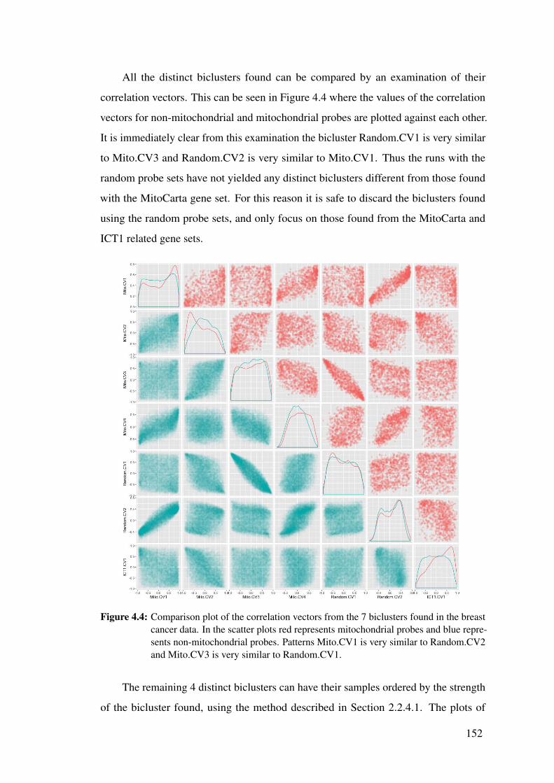
All the distinct biclusters found can be compared by an examination of their
correlation vectors. This can be seen in Figure 4.4 where the values of the correlation
vectors for non-mitochondrial and mitochondrial probes are plotted against each other.
It is immediately clear from this examination the bicluster Random.CV1 is very similar
to Mito.CV3 and Random.CV2 is very similar to Mito.CV1. Thus the runs with the
random probe sets have not yielded any distinct biclusters different from those found
with the MitoCarta gene set. For this reason it is safe to discard the biclusters found
using the random probe sets, and only focus on those found from the MitoCarta and
ICT1 related gene sets.
Figure 4.4: Comparison plot of the correlation vectors from the 7 biclusters found in the breastcancer data. In the scatter plots red represents mitochondrial probes and blue repre-sents non-mitochondrial probes. Patterns Mito.CV1 is very similar to Random.CV2and Mito.CV3 is very similar to Random.CV1.
The remaining 4 distinct biclusters can have their samples ordered by the strength
of the bicluster found, using the method described in Section 2.2.4.1. The plots of
152

these figures can be seen in Figure 4.5, where the samples are coloured according to
their PAM50 status. For biclusters Mito.CV1, Mito.CV2 and Mito.CV3, there is a clear
division between basal and luminal A tumour samples. Pattern ICT1.CV1 however
separates luminal A and B samples.
(a) Mito.CV1 (b) Mito.CV2
(c) Mito.CV3 (d) ICT1.CV1
Figure 4.5: PC1 plots of 4 biclusters found in the breast cancer data plots (a, b, c) show thethree remaining biclusters found from the MitoCarta gene set and (d) shows thebicluster found from the ICT1 related gene set. Samples are coloured according totheir PAM50 classification.
The MCbiclust method has therefore identified four potential biclusters describing
samples with expected mitochondrial differences. What is left to do is to quantify the
significance of the mitochondrial changes in this bicluster with gene set enrichment
analysis. This was done using Mann-Whitney test on GO terms as described in Sec-
tion 2.2.5.1 on the average correlation vectors of these biclusters. The top significant
gene set enrichment results can be seen in the Appendix in Tables B.13 to B.16, but
below in Table 4.2 are the significance of GO terms related to mitochondrial function in
all four of the biclusters.
153

GOID TERM ICT1.CV1adj p.value
Mito.CV1adj p.value
Mito.CV2adj p.value
Mito.CV3adjp.value
GO:0044429 mitochondrial part 5.569E-22 5.514E-04 4.048E-12 n.s.GO:0005739 mitochondrion 2.695E-21 4.290E-08 7.241E-14 n.s.GO:0005743 mitochondrial inner
membrane6.357E-17 n.s. 1.080E-09 n.s.
GO:0005740 mitochondrial envelope 9.383E-13 n.s. 1.429E-06 n.s.GO:0005761 mitochondrial ribosome 4.955E-11 n.s. 6.311E-09 n.s.GO:0031966 mitochondrial mem-
brane8.467E-11 n.s. 6.497E-06 n.s.
GO:0005759 mitochondrial matrix 5.176E-10 n.s. 3.491E-06 n.s.GO:0044455 mitochondrial mem-
brane part1.409E-09 n.s. 9.435E-04 n.s.
GO:0005746 mitochondrial respira-tory chain
1.114E-07 n.s. n.s. n.s.
GO:0005747 mitochondrial respira-tory chain complex I
7.331E-07 n.s. n.s. n.s.
GO:0007005 mitochondrion organiza-tion
1.575E-06 n.s. 4.275E-05 n.s.
GO:0042775 mitochondrial ATP syn-thesis coupled electrontransport
2.921E-04 n.s. n.s. n.s.
GO:0006120 mitochondrial electrontransport, NADH toubiquinone
5.185E-04 n.s. n.s. n.s.
GO:0005762 mitochondrial large ri-bosomal subunit
1.213E-03 n.s. n.s. n.s.
GO:0006839 mitochondrial transport 4.307E-03 n.s. 4.032E-02GO:0006626 protein targeting to mi-
tochondrion5.066E-03 n.s. 3.059E-02 n.s.
GO:0070585 protein localization tomitochondrion
1.181E-02 n.s. 4.291E-02 n.s.
GO:0072655 establishment of pro-tein localization to mi-tochondrion
1.423E-02 n.s. n.s. n.s.
GO:0005763 mitochondrial small ri-bosomal subunit
1.613E-02 n.s. n.s. n.s.
Table 4.2: Significant mitochondrial related GO terms in biclusters found in the breast cancerdataset. n.s. = non significant.
Table 4.2 shows that the ICT1.CV1 correlation vector has the most significant
mitochondrial related GO terms. Surprisingly the Mito.CV3 correlation vector, which
has 313 significant GO terms (the top 200 are given in Table B.15), but none related to the
mitochondria. Meanwhile, the Mito.CV1 correlation vector only has the generic terms
154

mitochondrion and mitochondrion part significant. Of the correlation vectors found
using the MitoCarta gene set only Mito.CV2 has a large number of mitochondrial related
GO terms significant and these are all less significant than those from the ICT1.CV1
correlation vector. Interestingly, Figure 4.4 seems to show the the non-mitochondrial
probes in Mito.CV2 and Mito.CV3 are correlated, and indeed if the significant GO terms
in Tables B.14 (for Mito.CV2) and B.15 (for Mito.CV3) are studied, both share many
terms linked to cellular proliferation. In addition to these, Mito.CV2 has significant
mitochondrial terms while Mito.CV3 has many significant terms linked to the immune
system.
Further studying of the ICT1.CV1 bicluster shows the upper fork samples have
increased mitochondrial expression compared to the lower fork samples. This can be
seen in Table 4.3 when examining the average expression of the significant mitochondria
related GO terms and shows that the difference in expression is especially great in the
mitochondrial ribosome and respiratory chain.
Of the three identified suitable biclusters, ICT1.CV1 was chosen for further analysis.
ICT1.CV1 as can be seen in Table 4.2 is the bicluster with the most associated significant
mitochondrial changes. It is also the only bicluster that separates between luminal A
and B samples in the upper and lower fork, as is seen in Figure 4.5.
Of the other three biclusters, Mito.CV3 is unsuitable due to its lack of significant
mitochondrial alterations, and Mito.CV1 and Mito.CV2 have weaker associated mito-
chondrial changes compared with ICT1.CV1. Mito.CV1 and Mito.CV2 do however
seem to represent a distinct bicluster that involves mitochondrial alterations between
basal and non-basal tumour samples, and could be of interest for investigating further.
However this will not be done due to the mitochondrial changes not being as significant
as for ICT1.CV1 and the difference between basal and non-basal tumours being less
interesting as they are widely recognised to be molecularly distinct diseases (Reis-Filho
2011). Additionally, the involvement of luminal A and B samples in ICT1.CV1 may
mean that this bicluster is relevant for determining which tumours do not benefit from
chemotherapy, a matter of current scientific interest (Stein et al. 2016).
155

GOID TERM Upper forkaverage
Lower forkaverage
GO:0005762 mitochondrial large ribosomal sub-unit
0.404 -0.249
GO:0005747 mitochondrial respiratory chaincomplex I
0.250 -0.138
GO:0005761 mitochondrial ribosome 0.237 -0.183GO:0005746 mitochondrial respiratory chain 0.223 -0.127GO:0006120 mitochondrial electron transport,
NADH to ubiquinone0.213 -0.108
GO:0042775 mitochondrial ATP synthesis cou-pled electron transport
0.198 -0.097
GO:0006626 protein targeting to mitochondrion 0.188 -0.094GO:0044455 mitochondrial membrane part 0.184 -0.076GO:0005763 mitochondrial small ribosomal sub-
unit0.147 -0.176
GO:0005743 mitochondrial inner membrane 0.144 -0.052GO:0070585 protein localization to mitochon-
drion0.128 -0.085
GO:0072655 establishment of protein localizationto mitochondrion
0.127 -0.081
GO:0006839 mitochondrial transport 0.111 -0.043GO:0044429 mitochondrial part 0.107 -0.022GO:0005740 mitochondrial envelope 0.107 -0.007GO:0031966 mitochondrial membrane 0.107 -0.005GO:0005759 mitochondrial matrix 0.107 -0.050GO:0007005 mitochondrion organization 0.095 -0.036GO:0005739 mitochondrion 0.080 0.002
Table 4.3: Differences in average expression in significant mitochondria associated GO termsbetween the upper and lower fork samples in bicluster ICT1.CV1, the upper andlower fork samples were selected using the threshold function in MCbiclust.
4.2.4 Mutational alterations behind the bicluster
The additional data in the breast cancer dataset contains two sources that may help to
explain the underlying cause of the ICT1.CV1 bicluster. This is the genetic information
present in the copy number and mutational data.
The copy number data measured by CGAN (2012) on Affymetrix 6.0 single nu-
cleotide polymorphism (SNP) arrays across 773 tumour samples, 499 of which corre-
spond to one of the 522 primary cancer samples with measured mRNA levels. Genomic
Identification of Significant Targets in Cancer 2.0 (GISTIC2.0), was used to calculate
the somatic copy number alterations, in terms of deletion or amplification, for each gene
(Mermel et al. 2011).
156

The somatic mutational data was obtained by CGAN (2012) from whole exomic
sequencing of 510 tumours, identifying across the dataset mutations in 14130 unique
genes. 463 of the samples in this dataset correspond to one of the 522 primary cancer
samples with measured mRNA levels.
For the copy number dataset, the average copy number value for every gene was
calculated for samples belonging in the upper and lower fork, as decided by the threshold
biclustering algorithm described in Section 2.2.6, and also for the luminal A and B
samples. Following this the copy number difference, between groups can be calculated,
and regions where there is a significant difference found.
Of particular interest is the difference in copy number alterations between the
upper/lower fork and luminal A/B samples. This will show for instance if there is any
copy number alterations between two luminal B samples, one a member of the upper fork
and one not. Similarly, this can also be done for two luminal A samples, one a member
of the lower fork and one not. Figure 4.6(a) show the average copy number difference
between upper and lower fork samples for every gene plotted against the average copy
number differences between luminal A and B samples. There is a general trend that
copy number alterations while occurring in similar locations are greater between the
upper and lower fork samples, with a regression analysis showing that the average copy
number change between luminal A and B samples is roughly 30% that between the
upper and lower fork samples.
Figure 4.6(b) shows the average copy number difference between upper and luminal
B samples plotted against that of the difference between lower and luminal A samples.
From this figure it is apparent that in certain locations, upper fork samples have a much
higher copy number than luminal B samples, while lower fork samples have a decrease
copy number compared to luminal A samples. Thus in this way the change between
upper and lower fork samples that is seen in Figure 4.6(a) is maximised.
To find the significant copy number alteration regions, a permutation test was used
that took the sample groups and randomly reassigned them into groups of the same size.
This was repeated 100 times to get a estimated probability distribution of copy number
alterations expected by chance, and those regions with an adjusted p-value of less than
0.05 selected as significant.
Table 4.4 shows the regions with significant differences between the different
157

(a) (b)
Figure 4.6: Copy number alterations between upper/lower and luminal A/B in the ICT1.CV1bicluster, with each point representing the average copy number change of one geneover the samples. Figure (a) shows a scatter plot of the difference between the upperand lower samples against the difference between luminal A and B samples, withthe dashed line representing y = x and the red line representing the regression linewith equation y = 0.003+0.3⇥ x and adjusted r-squared value of 0.7877 . Figure(b) shows a scatter plot of the difference between upper and luminal B against thatbetween lower and luminal A samples, with the dashed lines representing linesy = 0 and x = 0 and the red line representing the regression line with equationy =�0.02�0.369⇥ x and adjusted r-squared value of 0.4833.
groups. Two large regions stand out, one on chromosome 8 and the other on chromosome
17. The region on chromosome 8, has a significantly lower average copy number in the
lower fork samples than the luminal A, while an overlapping region has a significantly
higher average copy number in the upper fork samples than the luminal B. A similar
effect also seems to occur on a small region on chromosome 11. The chromosome 17
region has a significantly lower average copy number in the lower fork samples but is
not significantly changed between the upper fork and luminal B samples.
For the somatic mutational data the vast majority of the mutations occur infrequently.
6398 of the 14130 found mutated genes only occur once in the dataset, and only 16
mutations occur in over 5% of the tumours. The most common mutation is in the
PIK3CA gene and is present in 38.4% of the tumours.
The hypergeometric test was used to test for significant differences between the
groups. Four comparisons were tested, upper-lower, upper-luminal B, lower-luminal A
158

Numberofgenes
Cytoband Location LumAaver-age
Lowerforkaver-age
Copychange
457 8q11.1 to 8q24.3 0.48 0.14 0.3414 11q13.3 0.43 0.17 0.2551 17q21.32 to 17q21.33 0.17 -0.04 0.214 17q22 0.14 -0.06 0.202 17q22 0.16 -0.03 0.18110 17q22 to 17q24.2 0.19 -0.05 0.2511 17q24.3 to 17q25.1 0.13 -0.07 0.201 17q25.1 0.13 -0.07 0.218 17q25.1 0.13 -0.07 0.2016 17q25.1 0.12 -0.07 0.1926 17q25.1 0.11 -0.07 0.1821 17q25.2 17q25.3 0.10 -0.07 0.1788 17q25.3 0.08 -0.07 0.161 20q13.2 0.39 0.08 0.31
Numberofgenes
Cytoband Location LumBaver-age
Upperforkaver-age
Copychange
227 8q21.12 to 8q24.22 0.99 1.88 0.894 8q24.3 0.79 1.67 0.882 11q13.3 1.51 1.77 -0.267 11q13.3 1.44 1.82 0.38
Table 4.4: Significant regions of copy number alterations between luminal A and lower forksamples and luminal B and upper fork samples. All genes in the significant regionsare significant with adjusted p-value < 0.05.
and luminal B-luminal A, with only the 16 genes that were mutated in more than 5% of
the total number of tumours tested for significance.
The results of this can be seen in Table 4.5 showing that 4 genes were significantly
different between the groups. The proportion of mutated samples for genes PIK3CA,
MAP3K1 and TP53 were found to be significant between luminal A and luminal B
samples, while mutations in CDH1 were found to be significant between Upper and
Lower fork samples, with this mainly being driven by CDH1 mutations occurring much
more frequently in lower fork samples than luminal A samples.
Overall the percentage difference between the frequency of the mutations between
the upper and lower forks was greater than that between the luminal A and B samples for
all 4 of these genes. However due to the still relative low frequency of these mutations
and the few numbers of upper and lower fork samples compared to luminal A and
B, only the difference in PIK3CA and CDH1 was found to be statistically significant
between the upper and lower fork.
159

PIK3CA CDH1 MAP3K1 TP53All mutations 196 (38.43%) 34 (13.14%) 67 (6.67%) 192 (37.65%)
LumA mutations 110 (52.63%) 22 (10.53%) 55 (26.32%) 24 (11.48%)Lower mutations 21 (60%) 11 (31.43%) 12 (34.29%) 1 (2.86%)LumB mutations 38 (18.18%) 6 (2.87%) 8 (3.83%) 38 (18.18%)Upper mutations 4 (18.18%) 0 (0%) 1 (4.55%) 6 (27.27%)
LumA% - LumB % 34.45 7.66 22.49 -6.70Adj p-value 7.55e-03 0.496 1.52e-04 2.46e-05
Lower% - Upper % 41.82 31.43 29.74 -24.42Adj p-value 0.0239 0.0294 0.0900 0.109
Lower% - LumA % 7.37 20.9 7.97 -8.63Adj p-value 1 0.00262 1 0.680
Upper% - LumB % 0 -2.87 0.718 9.09Adj p-value 0.699 1 1 1
Table 4.5: Somatic mutations in genes PIK3CA, CDH1, MAP3K1 and TP53. Top half of thetable shows number of samples with mutations in these genes, with the percentage ofsamples with mutated genes given in brackets. The bottom half of the table showsthe difference in mutation percentage between that upper/lower fork and luminal A/Bsamples, and the associated p-values of these differences.
Overall the results of studying the mutational data in terms of somatic mutation
frequency and copy number alterations suggest that the genomic differences between
the upper and lower fork samples is greater than that between luminal A and luminal B.
This in turn suggests that it is these genetic differences that are driving this bicluster.
4.3 Identification of a similar bicluster in a breast can-
cer cell line dataset
4.3.1 The data
Since the breast cancer tumour samples matching this bicluster are not available for
further functional studies, it would be helpful to identify breast cancer derived cell lines
which can be used as a model. This however presents challenges in how to obtain the
cell lines that most closely resemble the type of regulation identified. Therefore before
any experimental work can be undertaken, cell lines derived from breast cancer tissue
must be selected, that match the bicluster identified.
For this purpose a dataset by Neve et al. (2006) was used that contains gene
expression data for 51 breast cancer cell lines measured with Affymetrix GeneChip
Human Genome HG-U133A. This dataset was collected to attempt to model the diverse
160

range of transcriptomic profiles identified in breast cancer, and the 51 cell lines were
shown to mirror the expression of 145 primary breast tumour samples (Neve et al. 2006).
As such this dataset should contain breast cancer cell lines that mirror the expression
that has been identified in the bicluster ICT1.CV1.
This dataset only contained 51 samples so is unsuitable for use with the MCbiclust
methods. Furthermore new biclusters are not being sought in this dataset, but cell
lines that match the previous mitochondrial related bicluster, ICT1.CV1 identified in
Section 4.2.3. To complete this purpose, a new method has to be derived.
4.3.2 Point Scoring algorithmSince the correlation vector for the ICT1 related bicluster is known, this can be used as
the basis for finding similar biclusters in other datasets. In theory, genes with positive
correlation vector values should all be up-regulated together while those with negative
values are down-regulated and vice-versa. A point scoring algorithm can be devised that
calculates in a sample how many of the positive correlation vector genes are up-regulated
together at the same time as the negative correlation vector genes are down-regulated
together.
The algorithm is simple and works as follows:
1. Take two groups of genes A and B, with A all having positive correlation vector
values and B all having negative correlation vector values.
2. The gene expression data is normalised by median centering for each gene, and
give each sample an initial score of 0.
3. For each sample +1 is added to the score for every gene in A greater than 0, and
every gene in B less than 0.
4. For each sample �1 is added for every gene in A less than 0 and every gene in B
greater than 0.
A high positive score indicates that samples have the majority of the gene in set
A upregulated while the genes in set B are downregulated. A high negative score in
contrast indicates that samples have genes in set A down-regulated while genes in set B
are up-regulated. P-values can be calculated using permutation tests that recalculate the
point score but with randomly assigning the genes in A and B.
161

To demonstrate the use of this algorithm, for the breast cancer data, the point score
was calculated for each sample based on the genes in the ICT1 related gene set, divided
into two sets based on their correlation vector values. As can be seen in Figure 4.7, the
point score values greatly match that of the first principal component.
In this case positive values represent the lower fork samples, and negative values
represent the upper fork samples.
(a) (b)
Figure 4.7: Comparison between the point score values and PC1 of the ICT1.CV1 bicluster,where the point score has been calculated from the genes in the ICT1 related geneset. (a) shows a scatter plot of PC1 against the point score values (b) shows thepoint score values plotted against the ranking of the samples. This produces thesame fork pattern that can be seen in Figure 4.5 (b). In both plots the samples arecoloured according to their PAM50 classification.
4.3.3 Selecting breast cancer cell linesThe point scoring algorithm was applied on the breast cancer cell line dataset, using the
genes in the ICT1 related gene set divided into two groups A and B based on the sign of
their corresponding correlation vector values. The result of this can be seen in Table 4.6
with the corresponding adjusted p-values.
Many of the different cell lines were significant, but not all were easily available for
experimental work. MCF7, HCC202, and MDAMB453 were chosen as representatives
of the upper fork, while MDAMB436 and HS578T were chosen as representatives of
the lower fork. While BT474 was selected as a possible control, belonging to neither the
upper or lower fork.
Since the lower fork was found to be closely related to the luminal A subtype and
the upper fork is closely related to the luminal B subtype, it is of interest to identify
162

CellLine PointScore
AdjPvalue
Subtype
SUM44PE 237 0.00E+00 LuHCC70 223 2.40E-09 BaAHCC1187 217 5.03E-10 BaAHCC1143 193 0.00E+00 BaASUM185PE 173 7.99E-07 LuMDAMB436* 169 3.71E-09 BaBBT549 125 2.19E-03 BaBHCC2185 125 4.27E-04 LuSUM52PE 119 3.30E-05 LuMDAMB468 115 4.39E-01 BaA600MPE 105 2.13E-04 LuUACC812 105 4.21E-01 LuHCC1007 95 1.67E-02 LuZR7530 93 3.03E-05 LuSUM190PT 83 9.13E-01 BaASUM225 75 1.00E+00 BaAHS578T* 71 3.85E-04 BaBHCC1937 67 1.00E+00 BaAMDAMB415 63 2.46E-02 LuHCC38 57 1.00E+00 BaBHCC1569 45 2.46E-02 BaAHCC2157 45 9.86E-01 BaAMDAMB231 37 1.00E+00 BaBSUM1315MO2 35 7.85E-02 BaBBT20 23 1.00E+00 BaASUM149PT 23 1.00E+00 BaBBT474* 17 1.00E+00 LuMDAMB175VII 17 9.86E-01 Lu
CellLine PointScore
AdjPvalue
Subtype
ZR75B -287 2.59E-31 LuLY2 -267 1.96E-20 LuT47D -217 3.35E-11 LuHCC1428 -209 5.26E-13 LuCAMA1 -191 7.99E-07 LuMDAMB361 -179 6.69E-14 LuMDAMB453* -175 1.17E-08 LuHCC202* -165 1.34E-03 LuMCF7* -157 6.55E-07 LuMDAMB157 -133 3.82E-07 BaBBT483 -95 2.59E-06 LuMCF12A -77 2.16E-05 BaBMCF10A -53 4.13E-03 BaBHCC1500 -47 4.48E-04 BaBSKBR3 -45 1.00E+00 LuMDAMB435 -43 1.00E+00 BaBHCC1954 -37 1.00E+00 BaAHBL100 -33 1.00E+00 BaBSUM159PT -31 1.00E+00 BaBAU565 -21 1.00E+00 LuZR751 -17 1.00E+00 LuHCC3153 -15 1.00E+00 BaAMDAMB134VI -7 1.00E+00 Lu
Table 4.6: Point Scores calculated for the breast cancer cell lines from Neve et al. (2006). Thesubtype of each cell line is based on the classifications made by Neve et al. (2006),into one of three groups Luminal, BasalA and BasalB. Significant (adjusted p-vale< 0.05) positive point score cell lines are coloured blue and significant negative pointscore cell lines are coloured red. Breast cancer cell lines that were available forexperimental work are denoted with an asterix (⇤).
the subtype of the cell lines. Neve et al. (2006) attempted to classify them, using the
same methodology as is used for the PAM50 classifications, but only identified three
groups Luminal, Basal A and Basal B. These clearly are not the same standard groups
found through PAM50 (Parker et al. 2009). The PAM50 classifier itself cannot be used
on these samples since it is trained on breast cancer tumour data to find known breast
cancer tumour subtypes.
Identifying the breast cancer intrinsic subtypes in cell lines has proved to be a more
difficult than expected task. Recently Prat et al. (2013) tried to identify breast cancer
163

cell lines that represented all the known subtypes and surprisingly they could find no cell
line that matched the luminal A subtype. Prat et al. (2013) hypothesised that this was
due to most breast cancer cell lines being derived from metastatic tumours more likely
to be the luminal B subtype, and that luminal A tumours in general were unsuitable for
cell culture. Another hypothesis could be that the PAM methodology fails to identify
luminal A cell lines. ICT1.CV1, the mitochondrial related bicluster whose lower fork is
strongly related to the luminal A subtype, has here been used to identify cell lines that
are seemingly similar to this luminal A subtype, at least in terms of the expression of
the genes in the bicluster. It is possible that this method has identified luminal A cell
lines where the PAM method has failed.
4.4 Experimental study of mitochondrial function in
different breast cancer cell lines
4.4.1 Methodology
4.4.1.1 Cell culture
A laminar flow cabinet was used for all cell culture, this was so a sterile environment
would be maintained. All items being placed into this cabinet were sprayed with 70%
ethanol. During all cell culture a lab coat and gloves were worn at all times, the gloves
being sprayed with 70% ethanol before being placed in the cabinet. Prior and after to
use the cabinet was cleaned using Virkon, and after use the cabinet was closed, airflow
switched off and sterilised with a UV light.
MCF7, HCC202, MDA-MB-436, Hs587t and BT474 cell lines were obtained from
Barts Cancer Institute, London. Cell lines were cultured in Dulbecco’s modified eagles
medium (DMEM) with 10% fetal bovine Serum (FBS) and Normocin (25mg/L) in 10cm
tissue culture treated sterile plates. All cell lines were cultured in a 37°C incubator set
with 5% CO2 and 95% humidity. All cell lines were passaged every 3-4 days using
Trypsin, when they were between 80% and 90% confluency.
To passage a cell line, all media was removed, and then the cells were washed with
phosphate buffered saline (PBS) (10ml). Then trypsin (0.25%, 2ml) was added to the
dish and the cells placed in the incubator for 1-2 minutes until the cells had begun to
lift from the plates. DMEM + FBS (4ml) was then added to the dish to inactivate the
164

trypsin and the resulting cell suspension was mixed with a pipette to ensure all cells
were dislodged. The cell suspension was centrifuged at 500g for 2 minutes to form a
cell pellet free of trypsin, which was resuspended in DMEM + FBS. The cell suspension
was then split at a 1:2 ratio in a fresh 10cm plate or counted to plate a particular number
of cells.
If the cells were to be counted 10µL of cell suspension were mixed with 10µL
of trypan blue and 10µL of this was pipetted onto a haemocytometer. Using a light
microscope on a 10x objective, the number of cells in each of the four corner sections
of the haemocytometer was made. An average of this count was calculated and is
multiplied by two to account for the dilution with trypan blue. An estimation of the
number of cells per ml can then be made by multiplying this value by 10000.
4.4.1.2 NanoString
Cell lines were grown in 10cm plates and total ribonucleic acid (RNA) was extracted
using the Qiagen RNeasy extraction kit, according to the manufacturer’s protocols.
Hybridisation of the reporter codeset and capture probeset to the sample RNA
was done using the nanostring nCounter Gene Expression Protocol, on RNA samples
quantified by NanoDrop to 50ng of total RNA in a maximum of 5uL of sample, incubated
in a thermocycler set to 65°C for 12 hours.
Once removed from the thermocycler the samples were proceeded immediately to
post-hybridization processing with the nCounter Prep Station.
The Prep Station was set up with the hybridized samples, sample cartridge, prep
plates and other components according to the nanostring nCounter Prep Station protocol.
The Prep Station once set up performs wash steps to remove excess probes and non-
target cellular transcripts. After washing the Target/Probe RNA complexes are eluted
off and are immobilized in the cartridge for data collection.
All consumable components required for processing samples on the Prep Station
are provided in the nCounter Master Kit, and after set up no further action is required by
the user.
Once complete, the cartridge from the Prep Station can be analysed by the nCounter
Digital Analyzer. Before analysis the reporter library file associated with the Codeset is
uploaded onto the digital analyzer. Following that a cartridge definition file is created
165

that contains the sample information for the cartridge to be run.
The cartridge was placed within the Digital Analyzer and run according to the
instructions in the nCounter Digital Analyzer protocol. The Digital analyser using a
microscope objective and a charge-coupled device (CCD) camera, creates a digital
image from which hundreds of thousands of target molecule counts are made. These are
processed by the digital analyser and counts are tabulated into a comma separated value
(CSV) format.
4.4.1.3 Western blots
A Qiagen bicinchoninic acid (BCA) protein quantification kit was used to quantify
protein samples following the manufacturers instructions. Samples were then prepared
with loading buffer and denatured by boiling as appropriate per antibody (for the
MitoProfile cocktail antibody this was for 10 minutes at 60°C). 20µg protein per well
were loaded into 4-12% BisTris NuPAGE gels at 150V in MOPS running buffer until the
samples reached the bottom of the gel. Transfer buffer was used to pre-soak the blotting
pads. PVDF membranes were then cut to size, activated in methanol then soaked in
transfer buffer. The transfer apparatus was assembled and using a wet system at 30V for
2 hours gels were transferred onto a PVDF membrane. Ponceau-S was used to check the
protein transfer and then membranes were blocked for one hour at room temperature in
Tris-buffered saline (TBS)(Tris 0.5M - NaCl 1.5M)- Tween 0.1% and 5% milk. Using
appropriate dilutions the primary antibodies were applied overnight at 4°C. Membranes
were washed 3 times for 5 minutes each time with TBS-Tween before use of a suitable
horseradish peroxidase-conjugated secondary antibody for 1 hour at room temperature
in TBS-Tween and 5% milk. Then membranes were washed 3 times for 5 minutes each
time using TBS-Tween and imaged on a BioRAD ChemiDoc system using BioRAD
ECL. When a loading control was needed, the membranes were washed once more 3
times for 5 minutes each with TBS-Tween before the primary and secondary antibody
steps were repeated using an appropriate loading control (usually beta-actin). ImageJ
(https://imagej.nih.gov/ij/) was used to analyse the resulting images and
relative intensities were normalised to the loading controls.
166

4.4.1.4 Oroboros
Oxygen consumption rates were measured using an Oroboros Oxygraph-2k high resolu-
tion respirometry system (Oroboros Instruments, Innsbruck, Austria). Cells were grown
to confluency in 10cm plates for 48 hours prior to the assay. The cells were trypsinized,
and counted so they could be diluted to 1 million cell/ml in a respiration buffer (DMEM
powder (8.3g/L), sodium pyruvate (110mg/L), glucose (1000mg/L), Glutamax 100x
(10ml/L, final concentration 2mM), Sodium bicarbonate (3.7g/L), FBS 10% and media
adjusted to 7.4pH and filter sterilised with a 0.22 Stericup). Prior to the assay, electrode
air calibration was performed with the respiration buffer, as suggested by manufacturer’s
protocol. 2ml of the cell suspension were added to each of the two chambers, and
the O2 flow signal allowed to stabilise to the basal respiration rate. Drugs were added
to the chambers using Hamilton syringes at the following concentrations and order:
oligomycin (2.5µM), carbonylcyanide-p-(trifluoromethoxy)-phenylhydrazone (FCCP)
(titrated 1µ l at a time from a 1mM stock, to produce maximal respiratory capacity), and
antimycin A (2.5µM).
Oligomycin inhibits adenosine triphosphate (ATP) synthase and therefore blocks
the main proton channel into the mitochondrial matrix, the resulting respiration rate is
due to the proton leak in the inner mitochondrial membrane. FCCP uncouples the inner
mitochondrial membrane allowing protons to freely pass across the membrane. This
equalises the mitochondrial membrane potential but also leads to the flow of electrons
in the ETC not being dependent on the number of protons in the mitochondrial matrix.
This results in a maximal respiration rate where the ETC is not limited by the number
of protons in the mitochondrial matrix. Antimycin A inhibits cytochrome C reductase
otherwise known as Complex III in the ETC. This stops all oxygen consumption from
the mitochondrial and gives us a value for non-mitochondrial respiration that can be
subtracted from the basal, leak and maximal rates to give mitochondrial specific rates.
Data were then extracted and analysed using O2K cell analysis template to give
oxygen consumption per unit cells. Significance between different groups was then
tested by one-way analysis of variance (ANOVA).
167

4.4.1.5 Gas chromatography mass spectrometry (GC-MS)
Cells were grown as described in cell culture methods but with carbon-13 labelled
glucose/galactose added to the media.
Before metabolite extraction, cell plates were taken to a cold room 500µL of
medium from each plate was put into 1.5mL tubes, for later analysis, and frozen. The
remaining media was removed and the plates placed in an ice/water bath before washing
two times with 5ml of ice-cold PBS.
To extract the metabolites the following process was used: 800µL ice-cold
methanol, containing an internal standard of 1mM scyllo-inositol, was added to the
plates; cells were then detached from the plate by scraping with a cell scraper. This
mixture was added to a 15ml tube, and the plate then washed with 400µL of methanol
and 400µL of H2O which was also added to the tube. Then 400µL of ice-cold chlo-
roform was added to each tube. The tubes were placed in a water bath sonicator in a
cold room for one hour, with 3x8 minute pulses of sonication and then centrifuged for
10 minutes at 16,000rpm at a temperature of 0°C. The supernatant was extracted and
dried in a vacuum concentrator. The cell pellet was then re-extracted with 200µL of
methanol and 100µL of H2O, this was sonicated, spun and the supernatant added to
previous supernatant tube and dried again in a vacuum concentrator. The remaining
cell pellet was used for estimating dry weight and measuring total protein. The dried
supernatant was resuspended in 50µL chloroform, 150µL methanol and 150µL H2O
and spun for 5 minutes at 0°C and 16,000rpm. The extract is then in a biphasic partition,
with the upper phase containing the polar metabolites and the lower phase containing
lipidic metabolites. The polar phase portions of each extract were then transferred to
GC-MS vial inserts and dried in a vacuum concentrator. Separate vial inserts had 10µL
of the saved cell culture medium added, with 1mM scyllo-inositol, which were also
dried in a vacuum concentrator. Each vial insert then had 30µL of methanol added,
containing 1µL of 5mM nor-leucine as another internal standard, followed by 30µL of
methanol without nor-leucine, with the vials being dried in a vacuum concentrator after
each addition.
Before running samples on the mass spectrometer, derivatiation was done to im-
prove GC separation. 20µL methoxyamine (30mg/mL in pyridine) was added to each
insert and this was vortexed briefly and then incubated at room temperature overnight,
168

Silylation was then done by adding 20µL of BSTFA + TCMS reagent to each inset and
incubating for 1 hour at room temperature.
An Agilent 7890A GC with a 5975C triple axis detector MSD (Agilent Technolo-
gies, Santa Clara, CA) was used to analyse the samples. Metabolites were separated
on an Agilent J&W 122-5532G DB-5ms capillary column (30m x 0.25mm, 0.25µm
film thickness), in splitless mode. The injector and transfer line temperatures were 270
and 280°C, respectively. The flow rate of helium carrier gas was 0.7 mL/min. The
oven temperature was programmed to hold at 70°C for 2 min, increased to 295°C at a
12.5°C/min ramp rate, increased from 295°C to 320°C at a 25°C/min ramp rate, and
held at 320°C for 3 minutes. The mass spectrometer was operated in scan mode, after a
6 minute solvent delay with a range of 50�565 mass/charge (m/z) and a scan-rate of
2.8 scans per second.
Metabolites were identified by matching retention times and fragmentation patterns
to commercially available standards. Metabolite peaks were integrated at each isotopo-
logue m/z using MassHunter Workstation software (Agilent Technologies). Peak areas
were quantified based on peak areas of known standards using nor-leucine as an internal
standard, and then metabolite levels were normalised to protein content.
Mass isotopologues were stripped of the contribution from natural abundance,
based on the chemical formula of derivitised fragment quantified. Percent enrichment
for an isotopologue was calculated by dividing the corrected intensity by the sum of
corrected intensities of all isotopologues for that metabolite. Significance of metabolite
enrichment between different samples was calculated with one-way ANOVA.
4.4.1.6 Contributions
Experimental work was done in collaboration with others, the contributions of which
are described below. Michela Menegollo, a PhD student from Padova, Italy who is also
working in the Szabadkai lab contributed to the experimental work by extracting the
RNA used in the nanostring experiments and running all western blot experiments. The
Oroboros data was collected by myself in conjunction with Cathy Qin, an undergraduate
medical student at UCL whose experimental project I supervised. The GC-MS data was
collected in collaboration with Dr Mariia Yuneva at the Crick Institute, who helped with
the metabolite extraction, ran the samples on the mass spectrometer and assisted with
169

the data analysis.
4.4.2 Results
4.4.2.1 Transcriptomics with nanostring
The first task in investigating the mitochondrial functional properties of the cell lines
was to confirm that the transcriptional differences discussed in Section 4.2.3. This
was necessary due to the relatively high level of cell line misidentification in science
(American Type Culture Collection Standards Development Organization Workgroup
2010). By confirming that the cell lines match the expected regulation, we can be sure
that they are a true representation of the cell lines from the data collected by Neve et al.
(2006) used in Section 4.3.3.
Besides confirming the transcriptional differences, there is the opportunity to gain
more precise measurements than those available from microarrays. Microarrays are
inherently noisy and have a limited dynamical range and provide a measurement that
cannot be used to find the precise count of each transcript, or measure transcripts with
low copy numbers. For this reason a different method of measuring transcriptomics was
used.
RNA sequencing (RNA-seq) while a possible method was deemed not cost ef-
fective, while methods such as quantitative polymerase chain reaction (q-PCR) while
highly accurate is not high-throughput and impractical to measure a large number of
genes across many samples. Instead it was decided to measure mRNA transcripts with
Nanostring nCounter analysis system (Malkov et al. 2009) that has the accuracy of
q-PCR but the potential for high throughput measurements of hundreds of genes.
Nanostring chips only measure a select number of genes, in this case 172, so in
order to proceed with the transcriptomics, a 172 sized gene set had to be chosen to
measure. To choose the genes in the gene set several criteria were used. This gene
set needed to include genes from which the bicluster could be confirmed and other
transcripts that may be useful in determining other features of the sample such as those
involved in the transcription network, additionally nanostring required all genes to have
GenBankIDs.
Table 4.7 gives a brief overview of the main groups of genes included in the
nanostring gene set, along with a brief description of each one. Table C.1 in Appendix C
170

gives a full overview of all the genes in the nanostring dataset.
Gene group Description Numberofgenes
Transcription factor net-work
Chosen with reference to literature, see Hock(2009)
32
mtDNA The required GenBankIDs were from Jourdainet al. (2013).
10
p53-induced genes Chosen from Sen et al. (2011), p53 genes wereof particular interest for work on a separateproject not discussed in this thesis.
25
MitoCarta Total number of genes linked to the mitochon-dria.
61
Mitochondrial geneslinked to bicluster
Chosen due to the size of the log fold changebetween the upper and lower fork. 15 pre-dicted upregulated in the upper fork and 15predicted downregulated in the upper fork .
30
Non-mitochondrial geneslinked to bicluster
Chosen due to the size of the log fold changebetween the upper and lower fork. 14 pre-dicted upregulated in the upper fork and 15predicted downregulated in the upper fork.
29
Cytosolic ribosome Chose genes that encode cytosolic ribosomeproteins.
16
Mitochondrial ribosome Chose genes that encode mitochondrial ribo-some proteins
19
ETC Genes that are members of the electron trans-port chain.
20
Control Genes chosen for their lack of correlationto genes in the bicluster present at differingamounts.
4
Table 4.7: Groups of genes selected for the nanostring gene set. Note there is some overlap inthese groups, e.g. all 10 of the mtDNA genes are in the ETC.
From these measured mRNA transcripts a scoring system had to be derived to
judge whether the sample best matched the upper or lower fork group. A similar scoring
system to the point score system used in Section 4.3.2 was used, but limited to genes
measured by the nanostring probes. This scoring system was based on the regulation of
59 genes measured by the nanostring, chosen as 29 are up-regulated in the upper fork
and 30 downregulated in the lower fork. The 29 gene up-regulated in the upper fork
gene set will be referred to as gene set Up, and the 30 gene down-regulated gene set will
be referred to as gene set Down.
After normalising the counts to the median of each gene, the score is calculated
with four values
171

1. G1pos = |which(Up > 0)|
2. G1neg = |which(Up < 0)|
3. G2pos = |which(Down < 0)|
4. G2neg = |which(Down > 0)|
The score can then be calculated as follows:
Score =G1pos�G1neg�G2pos +G2neg
59(4.2)
With 59 being the total number of genes measured by nanostring for the means of
determining the classification of the sample.
The workings of this method can be demonstrated on the original breast cancer
microarray data (CGAN 2012). In a similar way to Section 4.3.2 with the scoring system
used to find the breast cancer cell lines, this nanostring scoring system when applied
on the breast cancer dataset, recreates the fork plot and the score values are strongly
correlated to that of the first principal component as can be seen in Figure 4.8.
(a) (b)
Figure 4.8: Comparison between the nanostring score values and PC1 the ICT1.CV1 bicluster.(a) shows a scatter plot of PC1 against the nanostring score values (b) shows thenanostring score values plotted against the ranking of the samples. This producesthe same fork pattern that can be seen in Figure 4.5(b). In both plots the samplesare coloured according to their PAM50 classification.
Additionally significance can be calculated using a permutation test in which the
genes in gene set Up and Down are randomly reassigned and the score recalculated.
172

This is repeated 10000 times to get an approximate distribution of the scores which is
then used to calculate the p-value.
Cell lines MCF7, HCC202 representing the upper fork and MDA436 and Hs587t
representing the lower fork had RNA extracted. Transcripts were measured using
nanostring in triplicate in the manner described in Section 4.4.1. The nanostring data
before analysis was normalised by subtracting the average of the negative control probes
as background then normalising to the average count number of the control genes.
Table 4.8 shows the nanostring score calculated from the nanostring data. This table
shows that all cell lines have significant scores are truly representatives of their respective
forks.
Cell Line Fork Replicate Nanostring Score Adj p-valueHCC202 Upper 1 0.49 9.566E-04HCC202 Upper 2 0.46 1.548E-03HCC202 Upper 3 0.36 2.054E-02Hs578t Lower 1 -0.73 2.339E-07Hs578t Lower 2 -0.59 4.253E-05Hs578t Lower 3 -0.69 1.245E-06MCF7 Upper 1 0.69 1.418E-06MCF7 Upper 2 0.49 9.516E-04MCF7 Upper 3 0.63 8.119E-06MDA436 Lower 1 -0.22 1.339E-01MDA436 Lower 2 -0.22 1.339E-01MDA436 Lower 3 -0.46 2.433E-03
Table 4.8: Nanostring scores for breast cancer cell lines
4.4.2.2 Western Blots
The cancer cell lines HCC202, MCF7, MDA453, MDA436, Hs587t and BT474 were
grown and the levels of mitochondrial proteins were measured using western blots.
The focus was on measuring members of the ETC to assess if there were any major
differences in the proteomics of this key mitochondrial pathway.
This was achieved using the MitoProfile antibody cocktail that measures one protein
from each complex of the ETC. For normalisation purposes three additional proteins
were measured b -tubulin a housekeeping gene, GRP-75 a mitochondrial heat shock
protein and GAPDH a protein involved in glycolysis. Thus the protein levels of the
ETC could be normalised to the mitochondria, glycolysis as well as a b -tubulin general
housekeeping gene.
173

Cell lines HCC202, MCF7 and MDA453 representing the upper fork and cell
lines MDA436 and Hs587t representing the lower fork and cell line BT474 which was
included as a control were all measured. A representative blot from this work is given in
Figure 4.9.
Figure 4.10 shows the summary of all the results after being quantified and tested
for significance. It was found that Complex I and IV are upregulated in the upper fork
cell lines compared with the lower fork cell lines when normalised to the general state
of the mitochondria with GRP-75. This confirms the results from the gene set analysis
of the ICT.CV1 bicluster which showed the expression of complex I and other members
of the respiratory chain were significantly up-regulated in upper fork samples, as can be
seen in Table 4.3.
Figure 4.9: Representative western blot of breast cancer cell lines MCF7, HCC202, MDA-453,MDA-436, Hs578t and BT474. Cell lines were measured after being grown asdescribed in the cell culture methods in Section 4.4.1.1. Upper fork cell lines arecoloured red, while lower fork cell lines are coloured blue and control cell lines arecoloured black. Note that HEK-293 is not a breast cancer cell line, but derived fromhuman embryonic kidney cells and was included in the blot as an alternative controlcell line from a different tissue of origin. Figure and blot were produced by MichelaMenegollo.
4.4.2.3 Oxygen Consumption
The respiratory state of the cell lines were tested to determine whether there is a
functional difference between the upper and lower fork cell lines. Mitochondria require
oxygen to produce ATP, so any differences between the oxygen consumption will
indicate functional differences in the workings of the ETC.
To do this the cell lines were grown and measured under different conditions on the
174

Figure 4.10: Summary of the western blots analysing protein levels of different ETC complexes.Red represents the average of the upper fork cell lines, blue the average of thelower fork cell lines, and black that of BT474, a control cell line. When normalisedto b -tubulin there are no significant differences, however when normalised toGRP-75 a mitochondrial heat shock protein, there are significant differences in theprotein levels for complex I and IV, and when normalised to GAPDH a proteininvolved in glycolysis only complex I is significant, figure produced by GyorgySzabadkai.
Oroboros. Three states were measured first a basal rate of oxygen consumption, then the
leak state where ATP synthase is blocked and oxygen consumption comes from the small
amount of electron flow driven by the protons that can leak across the inner membrane.
After this the maximal state is measured by uncoupling the mitochondrial membrane.
Uncoupling refers to the state when protons can easily enter the mitochondrial matrix,
175

equalising the membrane potential and allowing electron flow in the ETC to not be
constrained by the proton gradient across the inner mitochondrial membrane.
Figure 4.11 shows the final results of the respirometry experiments showing that the
upper fork breast cancer cell lines had significantly higher respiration than the lower fork
cell lines. Thereby confirming the transcriptomic and proteomic differences affecting
the mitochondrial ETC have an effect on its functional role.
Figure 4.11: Differing oxygen consumption rates in the cancer cell lines, B = basal rate, L =leak rate and M = maximal rate. The difference between the upper and lower forkcell lines was found to be significant with a p-value < 0.05. Figure produced byGyorgy Szabadkai.
4.4.2.4 Metabolism
The metabolic fluxes through central carbon metabolism of the cell state was studied.
Cell lines HCC202, MCF7 and MDA453 representing the upper fork and cell lines
MDA436 and Hs587t representing the lower fork were grown in a medium containing
labelled carbon-13 glucose or carbon-13 glutamine and then the derived metabolites
were measured using gas chromatography mass spectrometry. This was done to give
more insight into the metabolomic differences between the upper and lower fork cell
lines besides the known mitochondrial alterations, particularly in regards to how glucose
and glutamine are utilised in the tricarboxylic acid (TCA) cycle. The main results from
this analysis are given in Figures 4.12 and 4.13.
The right side of Figure 4.12 shows how labelled glucose enters the TCA cycle
through Acetyl-CoA. This labels two carbon atoms in Acetyl-CoA and to all the follow-
176

ing intermediates, further rounds of the cycle can also produce +3 or +4 carbon labelled
intermediates. The right side of Figure 4.13 similarly shows how labelled glutamine is
metabolised through a-ketoglutarate.
To understand the efficiency of glucose and glutamine utilisation in the TCA cycle,
the fraction of labelled metabolites can be examined. In particular the reduction of non-
labelled (+0) metabolites can be examined, representing the average total incorporation
of labelled carbons from a particular substrate. Figures 4.12 and 4.13 show the reduction
of non-labelled metabolites and the fractional incorporation of labelled carbon in a
specific manner (from +1 to +n, n=the total number of carbons in a specific metabolite),
as an average for the lower and upper fork cell lines. For glucose, shown in Figure 4.12,
there is a greater reduction of non-labelled (+0) metabolites in the upper fork compared
to lower fork cell lines. For glutamine, shown in Figure 4.13, the opposite is seen as
there is a greater reduction of non-labelled (+0) in the lower fork compared to upper
fork cell lines. In both cases these reductions were found to be significant with p-values
< 0.05.
Therefore from these results we can conclude that the upper fork cell lines are more
dependent on glucose for their metabolism, while the lower fork cell lines are more
dependent on glutamine. This indicates that lower fork samples are producing more
energy via glutaminolysis, a process that has been associated to many types of cancer
(Medina 2001, Yuneva 2008).
4.5 ConclusionIn this chapter the MCbiclust biclustering method was applied to breast cancer tumour
samples. In accordance to the results of previous chapters this led to finding biclusters
whose samples had significant different regulation of the mitochondria between them.
Out of the biclusters found, the one with the most significant mitochondrial changes was
chosen for further investigation.
Within this bicluster, ICT.CV1, two groups of samples were found, one called the
upper fork that had significantly up-regulated mitochondrial genes compared with the
other group, called the lower fork. These groups seem to be comprised of subsets of the
luminal A and B subtypes of breast cancer as found by the PAM50 method. In this case,
the upper fork samples were a subset of luminal B and the lower fork samples were a
177

Figure 4.12: Results of mass spectrometry of cancer cell lines from glucose labelling, showingon the right how labelled glucose enters the TCA cycle, and on the left the utilisa-tion of metabolites aspartate, malate, and fumerate. All show greater utilisation ofthe carbon labelled glucose in the upper fork cell lines (in red) versus the lower forkcell lines (in blue), this can be seen in the differences of the fractional enrichmentfor metabolites with +1 or more labelled carbons. The fractional enrichment ofthe non-labelled +0 metabolites has had 1 subtracted from it before plotting sothat the fork with the greater reduction (the upper fork cell lines) has the greatestnegative score. Significant differences are labelled with an asterix and denotep-value < 0.05. Figure produced by Gyorgy Szabadkai.
subset of luminal A.
While there were clear and large overlap between luminal A and lower fork samples
as well as luminal B and upper fork samples, this relationship was not exact. There
were for example a small number of luminal B samples in the lower fork and luminal
A samples in the upper fork as well as luminal A/B samples that were not in either the
upper and lower fork. This shows that this method is not simply replicating the PAM50
classifications, and is possibly giving a better classification of cancer tumours.
Using additional genetic data from the breast cancer dataset as available from
CGAN (2012), the mutational differences between the upper and lower fork were found
to be significantly greater than that between luminal A and B samples for both copy
178

Figure 4.13: Results of mass spectrometry of cancer cell lines from glutamine labelling, show-ing on the right how labelled glutamine enters the TCA cycle, and on the leftthe utilisation of metabolites aspartate, malate, and fumerate. All show greaterutilisation of the carbon labelled glutamine in the lower fork cell lines (in blue)versus the upper fork cell lines (in red), this can be seen in the differences ofthe fractional enrichment for metabolites with +1 or more labelled carbons. Thefractional enrichment of the non-labelled +0 metabolites has had 1 subtracted fromit before plotting so that the fork with the greater reduction (the lower fork celllines) has the greatest negative score. Significant differences are labelled with anasterix and denote p-value < 0.05. Figure produced by Gyorgy Szabadkai.
number alterations and somatic mutations, as discussed in Section 4.2.4.
After this analysis was completed it was decided to attempt to experimentally test
samples representative of this bicluster. Since breast cancer tumour samples were not
available, cancer cell line representatives of this bicluster were identified with a novel
algorithm.
These cell lines were then obtained for experimental study. The first step was to
confirm the transcriptomic changes between the upper and lower fork samples with
nanostring, then it was shown that these transcriptomic changes corresponded with
proteomic changes in the mitochondria, particularly in terms of the proteins of the ETC,
Complex I and IV. Then this proteomic change was associated with a functional change
179

between the cell lines by examining the rate of oxygen consumpton, finding that upper
fork cell lines consume oxygen at a higher rate. Finally the metabolomics of the upper
fork and lower fork cell lines were examined, revealing that the upper fork cells were
more dependent on glucose in the TCA cycle while the lower fork cell lines were more
dependent on glutamine.
There are many directions in which this work can continue. For example a more
in depth look could be taken of the functional properties of the cell lines, such as by
examining their cell growth rates, mitochondrial membrane potential and metabolic
state. This is work that is currently being undertaken by other members of the Szabadkai
lab.
One important experiment to undertake would be to find whether the upper or lower
fork samples are more susceptible to chemotherapy with mitochondrial targeting drugs.
Another direction would be to use the nanostring chip scoring system in Section 4.4.2.1
to develop a method for classifying samples that match the bicluster. Finally it could
be tested whether incorporating knowledge of this bicluster improves breast cancer
prognosis scores.
What is perhaps more important than the specific results coming from study of this
bicluster, is the creation of a workflow pipeline, of identifying a bicluster of interest
using the MCbiclust methods, selecting cell lines that are representative of the bicluster
and finally experimental studies on these cell lines to gain greater understanding of
the regulation behind the bicluster. This generalised workflow can be applied to any
bicluster found in any type of cancer with a large enough number of suitable cancer cell
lines and is not limited to studying mitochondrial biogenesis.
The bioinformatic methods developed in this work have succeeded as aimed in
identifying mitochondrial based biclusters in the gene expression data within disease
biology. A further aim however was to use these methods to learn about the regulation
of mitochondrial biogenesis. Two breast cancer types with differences in mitochondrial
regulation have been shown to exist what is causing them is more difficult to find, and
must be the subject of future work. One thing that these results have shown is that
mitochondria are not regulated completely independently, and mitochondrial biogenesis
frequently as part of a much wider biological program such as cellular proliferation,
reaction to the immune response or response to the cold.
180

Chapter 5
Conclusions
The aim of this thesis was to develop methods to investigate the role of mitochondrial
biogenesis in disease.
As discussed in detail in the Introduction in Chapter 1, mitochondrial biogenesis is
a very complex process involving the coordination of the nuclear genome with hundreds
of copies of the mitochondrial genome scattered across the cell in the creation of
over 1000 proteins. Mitochondrial biogenesis exist as both a continuous underlying
process occuring in order to replenish mitochondria during standard mitochondrial
turnover, and as a dynamic process that can increase mitochondrial number in response to
environmental conditions. The mitochondrial proteome varies greatly between different
tissues, and this too is indicative of the varying nature of the regulation of mitochondrial
biogenesis.
Clearly due to its varying nature and our lack of a comprehensive understanding of
the system regulating mitochondrial biogenesis new tools are needed. There is however
greater urgency behind this due to the wide role mitochondria play in disease, and
the involvement of deregulation of mitochondrial biogenesis within these conditions.
Mitochondrial defects have long been known to occur in cancer, neuro-degeneration,
heart disease, diabetes and even ageing. The creation of novel tools to investigate
mitochondrial biogenesis thus will not only greatly increase our understanding of
mitochondria, but potentially reveal new targets and methods to treat these diseases.
The approach taken in this thesis to investigate mitochondrial biogenesis is with
bioinformatics, specifically by investigating a transcriptomic signature of mitochondrial
biogenesis. Using large gene expression datasets, focusing on those genes known to be
involved in the mitochondria a method to achieve this was created in Chapter 2.
181

The resulting method Massively Correlating Biclustering (MCbiclust), takes a gene
set of interest, in this case a mitochondrial related gene set. With this gene set, samples
in the dataset are found in which the average strength of the correlation of the genes in
the gene set are maximised. Further steps of the method involve ranking the samples
by how well they preserve this correlation and scoring every gene by the strength of its
correlation with the average expression of a group of genes that strongly correlate with
each other over the selected samples.
The end result of this method results in a ranking of samples and genes, from
which a precise bicluster can be thresholded, and the bicluster can be further analysed,
for instance using principal component analysis to divide the samples of the bicluster
into different forks and gene set enrichment analysis to find the significant GO terms
associated with the bicluster found.
This method is described in detail in Chapter 2 and what is more it is shown to
outperform alternative biclustering methods in finding these large scale biclusters that
resemble signs of mitochondrial biogenesis. This method is also found to be more
universal than a tool for investigating mitochondrial biogenesis when it is applied to a
bacterial E. coli dataset and found a bicluster representing the stalling of DNA replication
following treatment with an antibiotic norfloxacin.
This suitability of the method on bacterial data was another indication that it was
ideal for investigating a similar sized system, that of mitochondrial biogenesis in disease.
This investigation was first approached in Chapter 3 in which MCbiclust was applied on
a hypertrophic cardiomyopathy dataset and a cancer cell line dataset.
Hypertrophic cardiomyopathy (HCM) represents a thickening of the heart muscles,
is often undiagnosed and is one of the leading causes of sudden death in the young.
The MCbiclust method was applied to a RNA-Seq dataset of 146 samples, and
found a striking bicluster related to mitochondrial function that divided healthy control
samples into one fork and HCM samples into the other fork. This was a strong indicator
of a significant mitochondrial difference that is present in some control samples but
never in a disease samples. This bicluster was related to a down-regulation of mitochon-
drial genes corresponding to an up-regulation of cell proliferation genes in the healthy
control samples, the absence of this regulation in the HCM samples suggests a possible
mechanism by which HCM can occur.
182

Other mitochondrial biclusters were found in the HCM data involving only the
disease samples, these while involving different regulation of mitochondria did not also
involve these cell proliferation related genes, and absence of additional mutational or any
other clinical data meant that no further investigation of the meaning of these biclusters
could be undertaken.
The MCbiclust method was then applied to microarray data from the Cancer Cell
Line Encyclopedia (CCLE). Two different unique biclusters were found, only one which
was strongly related to mitochondrial function. This bicluster mainly seemed to be tissue
driven, representing differences between haematopoietic and lymphoid derived cell lines
and carcinoma derived cell lines. As with the HCM bicluster, along with mitochondrial
terms being significant, so were general cellular proliferation terms.
With the additional data in the CCLE dataset it was possible to study whether there
was any significant mutational or pharmacological differences between the samples rep-
resentative of each fork. In both cases significant regions of the copy number alterations
were found and pharmacological compounds which have significantly different effects.
The main issue with this analysis is that the differences appeared to be primarily
tissue driven. Differences between cancer cell lines derived from different tissue are
known to be very large and as such finding differences between them is not so surprising.
While this demonstrated the ability of MCbiclust to find mitochondrial based biclusters
in cancer data, it was decided that further investigation in the alterations of mitochondrial
biogenesis in cancer should be studied in only one cancer type at a time.
Chapter 4 was therefore aimed to study mitochondrial alterations in breast cancer.
This work identified a bicluster significantly related to mitochondrial function seemingly
related to the luminal A and luminal B subtypes found with PAM50. The samples in
this bicluster however had greater mutational differences than those between luminal A
and luminal B.
To understand the precise mitochondrial differences, cancer cell lines that were
representative of the bicluster were selected. These cell lines had their mitochondrial
differences experimentally verified using nanostring technology to measure mRNA
levels. In collaboration with other groups more functional differences were shown by
examining the proteomics, metabolomics and oxygen consumption levels.
The limitations of this work should be briefly discussed. There are two fundamental
183

issues with the MCbiclust algorithm. The first is that is when examining a data set it is
not known how many significant biclusters exist within it. Due to the combinatorially
large number of possibilities, no method could check them all, as such there will always
be a level of uncertainty about how many biclusters exist within a dataset, though this
can in some ways be taken into consideration by running the algorithm many times
with different random seeds and on different gene sets. There is certainly a bias in the
algorithm to find the largest possible bicluster while not finding smaller biclusters.
The second issue for MCbiclust is of one of performance, MCbiclust was not written
for speed and calculating large correlation matrices, a task that is needed to be done
thousands of times is very computationally expensive. As the R package currently exists,
it is functional especially when used in conjunction with high throughput computing
resources but there is certainly scope for improving its performance.
The other main limitation is the ability to understand the results of MCbiclust
itself. There is a very simple and obvious disconnect to the patterns that are identified
in these biclusters and the mechanisms that are causing them. In many data sets there
is a reliance on additional clinical data, and if this is lacking interpreting the biclusters
becomes very difficult, as was the case in Chapter 3 when examining HCM. With patient
samples in the absence of large amounts of clinical data, experimental models are ideally
needed. Finding an experimental model that matches a known bicluster however is a
long process in itself, as was seen in Chapter 4.
This work has ended with a novel bioinformatic method to investigate mitochon-
drial biogenesis fully established. Chapter 4 presents a work pipeline for finding a
bicluster of interest to selecting a relevant model and running experiments that could
be repeated in many different systems. Importantly the work had shown the potential
to improve treatment for disease. In the case of breast cancer there is a possibility
of creating a nanostring based assay to classify samples into this group and by doing
so possibly improving the determination of prognosis and deciding therapies. In the
case of hypertrophic cardiomyopathy the bicluster has suggested a possible means of
dysregulation that leads to the disease.
It is important to mention that the method MCbiclust developed has more general
applications than to mitochondrial biogenesis in disease, and seems particularly suitable
to bacterial datasets as was shown in the E. coli work in Chapter 2. However in the
184

investigation of mitochondrial biogenesis it is especially relevant.
It is feasible using this method and a dataset containing enough samples under
enough conditions to build an encyclopedia of the many modes of mitochondrial bio-
genesis and the co-regulation that exists with other non-mitochondrial pathways. Upon
doing so the different modes of mitochondrial biogenesis once found can be related to
the state of the transcription factor network underlying it, gaining us understanding of
the workings of that network. If this is achieved pathological modes of mitochondrial
biogenesis will be easily identified and understood and hopefully along with that insight,
treated.
185

Bibliography
Abdi, Herve & Williams, L. J. (2010), ‘Principal component analysis’, Wiley Interdisci-
plinary Reviews: Computational Statistics 2(4), 433–459.
Aguilar-Ruiz, J. S. (2005), ‘Shifting and scaling patterns from gene expression data’,
Bioinformatics 21(20), 3840–3845.
Ahlqvist, K. J., Hamalainen, R. H., Yatsuga, S., Uutela, M., Terzioglu, M., Gotz, A.,
Forsstrom, S., Salven, P., Angers-Loustau, A., Kopra, O. H. et al. (2012), ‘Somatic
progenitor cell vulnerability to mitochondrial DNA mutagenesis underlies progeroid
phenotypes in polg mutator mice’, Cell metabolism 15(1), 100–109.
Alaynick, W. A., Kondo, R. P., Xie, W., He, W., Dufour, C. R., Downes, M., Jonker, J. W.,
Giles, W., Naviaux, R. K., Giguere, V. et al. (2007), ‘ERRg directs and maintains the
transition to oxidative metabolism in the postnatal heart’, Cell metabolism 6(1), 13–24.
Allen, J. F. (1993), ‘Control of gene expression by redox potential and the requirement for
chloroplast and mitochondrial genomes’, Journal of Theoretical Biology 165(4), 609–
631.
Alon, U., Barkai, N., Notterman, D. A., Gish, K., Ybarra, S., Mack, D. & Levine,
A. J. (1999), ‘Broad patterns of gene expression revealed by clustering analysis of
tumor and normal colon tissues probed by oligonucleotide arrays’, Proceedings of the
National Academy of Sciences 96(12), 6745–6750.
Ambrus, A. M., Islam, A. B., Holmes, K. B., Moon, N. S., Lopez-Bigas, N., Benev-
olenskaya, E. V. & Frolov, M. V. (2013), ‘Loss of dE2F compromises mitochondrial
function’, Developmental cell 27(4), 438–451.
186

American Type Culture Collection Standards Development Organization Workgroup
(2010), ‘Cell line misidentification: the beginning of the end’, Nature Reviews Cancer
10(6).
Anders, Simon & Huber, W. (2010), ‘Differential expression analysis for sequence count
data’, Genome biol 11(10), R106.
Andersson, S. G., Zomorodipour, A., Andersson, J. O., Sicheritz-Ponten, T., Alsmark,
U. C. M., Podowski, R. M., Naslund, A. K., Eriksson, A.-S., Winkler, H. H. &
Kurland, C. G. (1998), ‘The genome sequence of Rickettsia prowazekii and the origin
of mitochondria’, Nature 396(6707), 133–140.
Andersson, Ulf & Scarpulla, R. C. (2001), ‘PGC-1-related coactivator, a novel, serum-
inducible coactivator of nuclear respiratory factor 1-dependent transcription in mam-
malian cells’, Molecular and cellular biology 21(11), 3738–3749.
Andres, A. M., Stotland, A., Queliconi, B. B. & Gottlieb, R. A. (2015), ‘A time to reap,
a time to sow: mitophagy and biogenesis in cardiac pathophysiology’, Journal of
molecular and cellular cardiology 78, 62–72.
Arany, Z., Lebrasseur, N., Morris, C., Smith, E., Yang, W., Ma, Y., Chin, S. & Spiegel-
man, B. M. (2007), ‘The transcriptional coactivator PGC-1b drives the formation of
oxidative type iix fibers in skeletal muscle’, Cell metabolism 5(1), 35–46.
Arsenijevic, D., Onuma, H., Pecqueur, C., Raimbault, S., Manning, B. S., Miroux, B.,
Couplan, E., Alves-Guerra, M.-C., Goubern, M., Surwit, R. et al. (2000), ‘Disruption
of the uncoupling protein-2 gene in mice reveals a role in immunity and reactive
oxygen species production’, Nature genetics 26(4), 435–439.
Aschrafi, A., Schwechter, A. D., Mameza, M. G., Natera-Naranjo, O., Gioio, A. E.
& Kaplan, B. B. (2008), ‘MicroRNA-338 regulates local cytochrome c oxidase IV
mRNA levels and oxidative phosphorylation in the axons of sympathetic neurons’,
The Journal of Neuroscience 28(47), 12581–12590.
Ashburner, M., Ball, C. A., Blake, J. A., Botstein, D., Butler, H., Cherry, J. M., Davis,
A. P., Dolinski, K., Dwight, S. S., Eppig, J. T. et al. (2000), ‘Gene ontology: tool for
the unification of biology’, Nature genetics 25(1), 25–29.
187

Baar, K., Song, Z., Semenkovich, C. F., Jones, T. E., Han, D.-H., Nolte, L. A., Ojuka,
E. O., Chen, M. & Holloszy, J. O. (2003), ‘Skeletal muscle overexpression of nu-
clear respiratory factor 1 increases glucose transport capacity’, The FASEB Journal
17(12), 1666–1673.
Baar, K., Wende, A. R., Jones, T. E., Marison, M., Nolte, L. A., Chen, M., Kelly, D. P. &
Holloszy, J. O. (2002), ‘Adaptations of skeletal muscle to exercise: rapid increase in
the transcriptional coactivator PGC-1’, The FASEB Journal 16(14), 1879–1886.
Baltzer, C., Tiefenbock, S. K. & Frei, C. (2010), ‘Mitochondria in response to nutrients
and nutrient-sensitive pathways’, Mitochondrion 10(6), 589–597.
Bardella, C., Pollard, P. J. & Tomlinson, I. (2011), ‘SDH mutations in cancer’, Biochim-
ica et Biophysica Acta (BBA)-Bioenergetics 1807(11), 1432–1443.
Barres, R., Osler, M. E., Yan, J., Rune, A., Fritz, T., Caidahl, K., Krook, A. & Zierath,
J. R. (2009), ‘Non-cpg methylation of the pgc-1a promoter through dnmt3b controls
mitochondrial density’, Cell metabolism 10(3), 189–198.
Barretina, J., Caponigro, G., Stransky, N., Venkatesan, K., Margolin, A. A., Kim, S.,
Wilson, C. J., Lehar, J., Kryukov, G. V., Sonkin, D. et al. (2012), ‘The cancer cell
line encyclopedia enables predictive modelling of anticancer drug sensitivity’, Nature
483(7391), 603–607.
Barrey, E., Saint-Auret, G., Bonnamy, B., Damas, D., Boyer, O. & Gidrol, X.
(2011), ‘Pre-microRNA and mature microRNA in human mitochondria’, PloS one
6(5), e20220.
Bastin, J., Aubey, F., Rotig, A., Munnich, A. & Djouadi, F. (2008), ‘Activation of
peroxisome proliferator-activated receptor pathway stimulates the mitochondrial
respiratory chain and can correct deficiencies in patients cells lacking its components’,
The Journal of Clinical Endocrinology & Metabolism 93(4), 1433–1441.
Benevolenskaya, Elizaveta V & Frolov, M. V. (2015), ‘Emerging links between E2F
control and mitochondrial function’, Cancer research 75(4), 619–623.
188

Bergmann, S., Ihmels, J. & Barkai, N. (2003), ‘Iterative signature algorithm for the
analysis of large-scale gene expression data’, Physical review E 67(3), 031902.
Blanchet, E., Annicotte, J.-S., Lagarrigue, S., Aguilar, V., Clape, C., Chavey, C., Fritz,
V., Casas, F., Apparailly, F., Auwerx, J. et al. (2011), ‘E2F transcription factor-1
regulates oxidative metabolism’, Nature cell biology 13(9), 1146–1152.
Bogacka, I., Xie, H., Bray, G. A. & Smith, S. R. (2005), ‘Pioglitazone induces mi-
tochondrial biogenesis in human subcutaneous adipose tissue in vivo’, Diabetes
54(5), 1392–1399.
Bolstad, B., Collin, F., Simpson, K., Irizarry, R. & Speed, T. (2004), ‘Experimental de-
sign and low-level analysis of microarray data’, International review of neurobiology
60, 25–58.
Bookout, A. L., Jeong, Y., Downes, M., Ruth, T. Y., Evans, R. M. & Mangelsdorf, D. J.
(2006), ‘Anatomical profiling of nuclear receptor expression reveals a hierarchical
transcriptional network’, Cell 126(4), 789–799.
Bozdag, D., Parvin, J. D. & Catalyurek, U. V. (2009), A biclustering method to discover
co-regulated genes using diverse gene expression datasets, in ‘Bioinformatics and
Computational Biology’, Springer, pp. 151–163.
Brand, Martin D & Nicholls, D. G. (2011), ‘Assessing mitochondrial dysfunction in
cells’, Biochemical Journal 435(2), 297–312.
Bratic, A., Larsson, N.-G. et al. (2013), ‘The role of mitochondria in aging’, The Journal
of clinical investigation 123(123 (3)), 951–957.
Calvo, S. E., Clauser, K. R. & Mootha, V. K. (2015), ‘MitoCarta2.0: an updated
inventory of mammalian mitochondrial proteins’, Nucleic acids research p. gkv1003.
Calvo, S., Jain, M., Xie, X., Sheth, S. A., Chang, B., Goldberger, O. A., Spinazzola,
A., Zeviani, M., Carr, S. A. & Mootha, V. K. (2006), ‘Systematic identification of
human mitochondrial disease genes through integrative genomics’, Nature genetics
38(5), 576–582.
189

Cam, H., Balciunaite, E., Blais, A., Spektor, A., Scarpulla, R. C., Young, R., Kluger, Y. &
Dynlacht, B. D. (2004), ‘A common set of gene regulatory networks links metabolism
and growth inhibition’, Molecular cell 16(3), 399–411.
Catic, A., Suh, C. Y., Hill, C. T., Daheron, L., Henkel, T., Orford, K. W., Dombkowski,
D. M., Liu, T., Liu, X. S. & Scadden, D. T. (2013), ‘Genome-wide map of nuclear
protein degradation shows NCoR1 turnover as a key to mitochondrial gene regulation’,
Cell 155(6), 1380–1395.
CGAN (2012), ‘Comprehensive molecular portraits of human breast tumours’, Nature
490(7418), 61–70.
Chan, J. Y., Kwong, M., Lu, R., Chang, J., Wang, B., Yen, T. B. & Kan, Y. W. (1998),
‘Targeted disruption of the ubiquitous CNC-bZIP transcription factor, nrf-1, results in
anemia and embryonic lethality in mice’, The EMBO Journal 17(6), 1779–1787.
Chan, S. Y., Zhang, Y.-Y., Hemann, C., Mahoney, C. E., Zweier, J. L. & Loscalzo,
J. (2009), ‘MicroRNA-210 controls mitochondrial metabolism during hypoxia by
repressing the iron-sulfur cluster assembly proteins ISCU1/2’, Cell metabolism
10(4), 273–284.
Chang, T.-C., Yu, D., Lee, Y.-S., Wentzel, E. A., Arking, D. E., West, K. M., Dang, C. V.,
Thomas-Tikhonenko, A. & Mendell, J. T. (2008), ‘Widespread microRNA repression
by Myc contributes to tumorigenesis’, Nature genetics 40(1), 43–50.
Cheng, Yizong & Church, G. M. (2000), Biclustering of expression data., in ‘Ismb’,
Vol. 8, pp. 93–103.
Chipuk, J., Bouchier-Hayes, L. & Green, D. (2006), ‘Mitochondrial outer membrane
permeabilization during apoptosis: the innocent bystander scenario’, Cell Death &
Differentiation 13(8), 1396–1402.
Ciriello, G., Sinha, R., Hoadley, K. A., Jacobsen, A. S., Reva, B., Perou, C. M., Sander,
C. & Schultz, N. (2013), ‘The molecular diversity of Luminal A breast tumors’, Breast
cancer research and treatment 141(3), 409–420.
190

Civitarese, A. E., Carling, S., Heilbronn, L. K., Hulver, M. H., Ukropcova, B., Deutsch,
W. A., Smith, S. R. & Ravussin, E. (2007), ‘Calorie restriction increases muscle
mitochondrial biogenesis in healthy humans’, PLoS med 4(3), e76.
Crick, F. . o. (1970), ‘Central dogma of molecular biology’, Nature 227(5258), 561–563.
Csardi, G., Kutalik, Z. & Bergmann, S. (2010), ‘Modular analysis of gene expression
data with R’, Bioinformatics 26(10), 1376–1377.
Cunningham, J. T., Rodgers, J. T., Arlow, D. H., Vazquez, F., Mootha, V. K. & Puigserver,
P. (2007), ‘mTOR controls mitochondrial oxidative function through a YY1–PGC-
1&agr; transcriptional complex’, nature 450(7170), 736–740.
Dang, C. V. (2012), ‘MYC on the path to cancer’, Cell 149(1), 22–35.
Dennis Jr, G., Sherman, B. T., Hosack, D. A., Yang, J., Gao, W., Lane, H. C., Lempicki,
R. A. et al. (2003), ‘DAVID: database for annotation, visualization, and integrated
discovery’, Genome biol 4(5), P3.
Dillies, M.-A., Rau, A., Aubert, J., Hennequet-Antier, C., Jeanmougin, M., Servant,
N., Keime, C., Marot, G., Castel, D., Estelle, J. et al. (2013), ‘A comprehensive
evaluation of normalization methods for illumina high-throughput RNA sequencing
data analysis’, Briefings in bioinformatics 14(6), 671–683.
Divakaruni, A. S., Rogers, G. W. & Murphy, A. N. (2014), ‘Measuring mitochondrial
function in permeabilized cells using the seahorse XF analyzer or a clark-type oxygen
electrode’, Current Protocols in Toxicology pp. 25–2.
Dominy, J. E., Lee, Y., Gerhart-Hines, Z. & Puigserver, P. (2010), ‘Nutrient-dependent
regulation of PGC-1a’s acetylation state and metabolic function through the enzy-
matic activities of Sirt1/GCN5’, Biochimica et Biophysica Acta (BBA)-Proteins and
Proteomics 1804(8), 1676–1683.
Dowsett, M., Sestak, I., Lopez-Knowles, E., Sidhu, K., Dunbier, A. K., Cowens, J. W.,
Ferree, S., Storhoff, J., Schaper, C. & Cuzick, J. (2013), ‘Comparison of PAM50 risk
of recurrence score with oncotype dx and ihc4 for predicting risk of distant recurrence
after endocrine therapy’, Journal of Clinical Oncology pp. JCO–2012.
191

Duchen, Michael R & Szabadkai, G. (2010), ‘Roles of mitochondria in human disease’,
Essays Biochem 47, 115–137.
Dufour, C. R., Wilson, B. J., Huss, J. M., Kelly, D. P., Alaynick, W. A., Downes, M.,
Evans, R. M., Blanchette, M. & Giguere, V. (2007), ‘Genome-wide orchestration of
cardiac functions by the orphan nuclear receptors ERRa and g’, Cell metabolism
5(5), 345–356.
Early Breast Cancer Trialists Collaborative Group (2005), ‘Effects of chemotherapy
and hormonal therapy for early breast cancer on recurrence and 15-year survival: an
overview of the randomised trials’, The Lancet 365(9472), 1687–1717.
Eisen, M. B., Spellman, P. T., Brown, P. O. & Botstein, D. (1998), ‘Cluster analysis and
display of genome-wide expression patterns’, Proceedings of the National Academy
of Sciences 95(25), 14863–14868.
Emanuelsson, O., Brunak, S., von Heijne, G. & Nielsen, H. (2007), ‘Locating proteins
in the cell using TargetP, SignalP and related tools’, Nature protocols 2(4), 953–971.
Epstein, C. B., Waddle, J. A., Hale, W., Dave, V., Thornton, J., Macatee, T. L., Garner,
H. R. & Butow, R. A. (2001), ‘Genome-wide responses to mitochondrial dysfunction’,
Molecular biology of the cell 12(2), 297–308.
Evans, R. M., Barish, G. D. & Wang, Y.-X. (2004), ‘PPARs and the complex journey to
obesity’, Nature medicine 10(4), 355–361.
Exner, N., Lutz, A. K., Haass, C. & Winklhofer, K. F. (2012), ‘Mitochondrial dysfunction
in Parkinson’s disease: molecular mechanisms and pathophysiological consequences’,
The EMBO journal 31(14), 3038–3062.
Faith, J. J., Driscoll, M. E., Fusaro, V. A., Cosgrove, E. J., Hayete, B., Juhn, F. S.,
Schneider, S. J. & Gardner, T. S. (2008), ‘Many microbe microarrays database:
uniformly normalized affymetrix compendia with structured experimental metadata’,
Nucleic acids research 36(suppl 1), D866–D870.
Fassone, Elisa & Rahman, S. (2012), ‘Complex I deficiency: clinical features, biochem-
istry and molecular genetics’, Journal of medical genetics 49(9), 578–590.
192

Feinberg, A. P. (2008), ‘Epigenetics at the epicenter of modern medicine’, Jama
299(11), 1345–1350.
Feinberg, Andrew P & Tycko, B. (2004), ‘The history of cancer epigenetics’, Nature
Reviews Cancer 4(2), 143–153.
Fisher, R. A. (1922), ‘On the interpretation of c2 from contingency tables, and the
calculation of p’, Journal of the Royal Statistical Society pp. 87–94.
Fletcher, Martin J & Sanadi, D. (1961), ‘Turnover of rat-liver mitochondria’, Biochimica
et biophysica acta 51(2), 356–360.
Foulkes, W. D., Flanders, T. Y., Pollock, P. M. & Hayward, N. K. (1997), ‘The CDKN2A
(p16) gene and human cancer.’, Molecular Medicine 3(1), 5.
Fulda, S., Galluzzi, L. & Kroemer, G. (2010), ‘Targeting mitochondria for cancer
therapy’, Nature reviews Drug discovery 9(6), 447–464.
Gakh, O., Cavadini, P. & Isaya, G. (2002), ‘Mitochondrial processing peptidases’,
Biochimica et Biophysica Acta (BBA)-Molecular Cell Research 1592(1), 63–77.
Gallo, C. A., Carballido, J. A. & Ponzoni, I. (2009), Bihea: A hybrid evolutionary ap-
proach for microarray biclustering, in ‘Advances in Bioinformatics and Computational
Biology’, Springer, pp. 36–47.
Gama-Castro, S., Salgado, H., Peralta-Gil, M., Santos-Zavaleta, A., Muniz-Rascado, L.,
Solano-Lira, H., Jimenez-Jacinto, V., Weiss, V., Garcıa-Sotelo, J. S., Lopez-Fuentes,
A. et al. (2011), ‘RegulonDB version 7.0: transcriptional regulation of escherichia
coli k-12 integrated within genetic sensory response units (gensor units)’, Nucleic
acids research 39(suppl 1), D98–D105.
Gao, P., Tchernyshyov, I., Chang, T.-C., Lee, Y.-S., Kita, K., Ochi, T., Zeller, K. I.,
De Marzo, A. M., Van Eyk, J. E., Mendell, J. T. et al. (2009), ‘c-Myc suppres-
sion of miR-23a/b enhances mitochondrial glutaminase expression and glutamine
metabolism’, Nature 458(7239), 762–765.
193

Garcıa-Prat, L., Martınez-Vicente, M., Perdiguero, E., Ortet, L., Rodrıguez-Ubreva, J.,
Rebollo, E., Ruiz-Bonilla, V., Gutarra, S., Ballestar, E., Serrano, A. L. et al. (2016),
‘Autophagy maintains stemness by preventing senescence’, Nature 529(7584), 37–42.
Garzon, R., Calin, G. A. & Croce, C. M. (2009), ‘MicroRNAs in cancer’, Annual review
of medicine 60, 167–179.
Gasch, Audrey P & Eisen, M. B. (2002), ‘Exploring the conditional coregulation of
yeast gene expression through fuzzy k-means clustering’, Genome Biol 3(11), 1–22.
Gerdes, F., Tatsuta, T. & Langer, T. (2012), ‘Mitochondrial aaa proteasestowards a
molecular understanding of membrane-bound proteolytic machines’, Biochimica Et
Biophysica Acta (BBA)-Molecular Cell Research 1823(1), 49–55.
Gerhart-Hines, Z., Rodgers, J. T., Bare, O., Lerin, C., Kim, S.-H., Mostoslavsky, R.,
Alt, F. W., Wu, Z. & Puigserver, P. (2007), ‘Metabolic control of muscle mitochon-
drial function and fatty acid oxidation through SIRT1/PGC-1a’, The EMBO journal
26(7), 1913–1923.
Giguere, V., Yang, N., Segui, P. & Evans, R. M. (1988), ‘Identification of a new class of
steroid hormone receptors’.
Giordano, S. H., Buzdar, A. U. & Hortobagyi, G. N. (2002), ‘Breast cancer in men’,
Annals of internal medicine 137(8), 678–687.
Gnaiger, E. (2007), ‘Mitochondrial pathways and respiratory control’, Textbook on
Mitochondrial Physiology, edited by E Gnaiger Innsbruck, Austria: OROBOROS
MiPNet pp. 1–95.
Gogvadze, V., Orrenius, S. & Zhivotovsky, B. (2008), ‘Mitochondria in cancer cells:
what is so special about them?’, Trends in cell biology 18(4), 165–173.
Griffiths-Jones, S., Grocock, R. J., Van Dongen, S., Bateman, A. & Enright, A. J. (2006),
‘miRBase: microRNA sequences, targets and gene nomenclature’, Nucleic acids
research 34(suppl 1), D140–D144.
194

Gugneja, Sajiv Scarpulla, R. C. (1997), ‘Serine phosphorylation within a concise amino-
terminal domain in nuclear respiratory factor 1 enhances DNA binding’, Journal of
Biological Chemistry 272(30), 18732–18739.
Hanahan, Douglas & Weinberg, R. A. (2000), ‘The hallmarks of cancer’, cell 100(1), 57–
70.
Hanahan, Douglas & Weinberg, R. A. (2011), ‘Hallmarks of cancer: the next generation’,
cell 144(5), 646–674.
Hancock, C. R., Han, D.-H., Higashida, K., Kim, S. H. & Holloszy, J. O. (2011), ‘Does
calorie restriction induce mitochondrial biogenesis? a reevaluation’, The FASEB
Journal 25(2), 785–791.
Handschin, C. (2009), ‘The biology of PGC-1a and its therapeutic potential’, Trends in
pharmacological sciences 30(6), 322–329.
Hara, E., Smith, R., Parry, D., Tahara, H., Stone, S. & Peters, G. (1996), ‘Regulation of
p16CDKN2 expression and its implications for cell immortalization and senescence.’,
Molecular and Cellular Biology 16(3), 859–867.
Harman, D. (1955), ‘Aging: a theory based on free radical and radiation chemistry’.
Hartigan, J. A. (1972), ‘Direct clustering of a data matrix’, Journal of the american
statistical association 67(337), 123–129.
Haybittle, J., Blamey, R., Elston, C., Johnson, J., Doyle, P., Campbell, F., Nicholson, R.
& Griffiths, K. (1982), ‘A prognostic index in primary breast cancer.’, British journal
of cancer 45(3), 361.
Haynes, Brian C & Brent, M. R. (2009), ‘Benchmarking regulatory network reconstruc-
tion with GRENDEL’, Bioinformatics 25(6), 801–807.
Hebl, V. B., Bos, J., Oberg, A. L., Sun, Z., Maleszewski, J. J., Ogut, O., Bishu, K., dos
Remedios, C. G., Ommen, S., Schaff, H. V. et al. (2012), ‘Transcriptome profiling of
surgical myectomy tissue from patients with hypertrophic cardiomyopathy reveals
marked overexpression of ACE2’, Circulation 126(21 Supplement), A11099.
195

Hekimi, S., Lapointe, J. & Wen, Y. (2011), ‘Taking a good look at free radicals in the
aging process’, Trends in cell biology 21(10), 569–576.
Herschkowitz, J. I., Simin, K., Weigman, V. J., Mikaelian, I., Usary, J., Hu, Z., Ras-
mussen, K. E., Jones, L. P., Assefnia, S., Chandrasekharan, S. et al. (2007), ‘Identifi-
cation of conserved gene expression features between murine mammary carcinoma
models and human breast tumors’, Genome biology 8(5), R76.
Herzig, S., Long, F., Jhala, U. S., Hedrick, S., Quinn, R., Bauer, A., Rudolph, D., Schutz,
G., Yoon, C., Puigserver, P. et al. (2001), ‘CREB regulates hepatic gluconeogenesis
through the coactivator PGC-1’, Nature 413(6852), 179–183.
Hirschey, M. D., DeBerardinis, R. J., Diehl, A. M. E., Drew, J. E., Frezza, C., Green,
M. F., Jones, L. W., Ko, Y. H., Le, A., Lea, M. A. et al. (2015), Dysregulated
metabolism contributes to oncogenesis, in ‘Seminars in cancer biology’, Vol. 35,
Elsevier, pp. S129–S150.
Hochreiter, S., Bodenhofer, U., Heusel, M., Mayr, A., Mitterecker, A., Kasim, A.,
Khamiakova, T., Van Sanden, S., Lin, D., Talloen, W. et al. (2010), ‘FABIA: factor
analysis for bicluster acquisition’, Bioinformatics 26(12), 1520–1527.
Hock, M Benjamin & Kralli, A. (2009), ‘Transcriptional control of mitochondrial
biogenesis and function’, Annual review of physiology 71, 177–203.
Hoitzing, H., Johnston, I. G. & Jones, N. S. (2015), ‘What is the function of mito-
chondrial networks? a theoretical assessment of hypotheses and proposal for future
research’, BioEssays 37(6), 687–700.
Holmgren, D., Wahlander, H., Eriksson, B., Oldfors, A., Holme, E. & Tulinius, M.
(2003), ‘Cardiomyopathy in children with mitochondrial disease clinical course and
cardiological findings’, European heart journal 24(3), 280–288.
Hondares, E., Mora, O., Yubero, P., de la Concepcion, M. R., Iglesias, R., Giralt,
M. & Villarroya, F. (2006), ‘Thiazolidinediones and rexinoids induce peroxisome
proliferator-activated receptor-coactivator (PGC)-1a gene transcription: an autoregu-
latory loop controls PGC-1a expression in adipocytes via peroxisome proliferator-
activated receptor-g coactivation’, Endocrinology 147(6), 2829–2838.
196

Horton, T. M., Petros, J. A., Heddi, A., Shoffner, J., Kaufman, A. E., Graham, S. D.,
Gramlich, T. & Wallace, D. C. (1996), ‘Novel mitochondrial DNA deletion found in
a renal cell carcinoma’, Genes, Chromosomes and Cancer 15(2), 95–101.
Huq, M. M., Gupta, P., Tsai, N.-P., White, R., Parker, M. G. & Wei, L.-N. (2006),
‘Suppression of receptor interacting protein 140 repressive activity by protein arginine
methylation’, The EMBO journal 25(21), 5094–5104.
Huss, J. M., Garbacz, W. G. & Xie, W. (2015), ‘Constitutive activities of estrogen-
related receptors: transcriptional regulation of metabolism by the ERR pathways in
health and disease’, Biochimica et Biophysica Acta (BBA)-Molecular Basis of Disease
1852(9), 1912–1927.
Irizarry, R. A., Hobbs, B., Collin, F., Beazer-Barclay, Y. D., Antonellis, K. J., Scherf, U.,
Speed, T. P. et al. (2003), ‘Exploration, normalization, and summaries of high density
oligonucleotide array probe level data’, Biostatistics 4(2), 249–264.
Ishikawa, K., Takenaga, K., Akimoto, M., Koshikawa, N., Yamaguchi, A., Imanishi, H.,
Nakada, K., Honma, Y. & Hayashi, J.-I. (2008), ‘ROS-generating mitochondrial DNA
mutations can regulate tumor cell metastasis’, Science 320(5876), 661–664.
Issemann, Isabelle & Green, S. (1990), ‘Activation of a member of the steroid hormone
receptor superfamily by peroxisome proliferators.’, Nature 347(6294), 645–650.
Ivanova, N., Dobrin, R., Lu, R., Kotenko, I., Levorse, J., DeCoste, C., Schafer, X.,
Lun, Y. & Lemischka, I. R. (2006), ‘Dissecting self-renewal in stem cells with RNA
interference’, Nature 442(7102), 533–538.
Jager, S., Handschin, C., Pierre, J. S. & Spiegelman, B. M. (2007), ‘AMP-activated
protein kinase (AMPK) action in skeletal muscle via direct phosphorylation of PGC-
1a’, Proceedings of the National Academy of Sciences 104(29), 12017–12022.
Johnson, L. V., Walsh, M. L. & Chen, L. B. (1980), ‘Localization of mitochondria in
living cells with rhodamine 123’, Proceedings of the National Academy of Sciences
77(2), 990–994.
197
Jones, A. W., Yao, Z., Vicencio, J. M., Karkucinska-Wieckowska, A. & Szabadkai, G.
(2012), ‘PGC-1 family coactivators and cell fate: Roles in cancer, neurodegeneration,
cardiovascular disease and retrograde mitochondria–nucleus signalling’, Mitochon-
drion 12(1), 86–99.
Jones, Peter A & Laird, P. W. (1999), ‘Cancer-epigenetics comes of age’, Nature genetics
21(2), 163–167.
Jourdain, A. A., Koppen, M., Wydro, M., Rodley, C. D., Lightowlers, R. N.,
Chrzanowska-Lightowlers, Z. M. & Martinou, J.-C. (2013), ‘GRSF1 regulates RNA
processing in mitochondrial RNA granules’, Cell metabolism 17(3), 399–410.
Kaiser, Sebastian & Leisch, F. (2008), ‘A toolbox for bicluster analysis in r’.
Kallen, J., Schlaeppi, J.-M., Bitsch, F., Filipuzzi, I., Schilb, A., Riou, V., Graham, A.,
Strauss, A., Geiser, M. & Fournier, B. (2004), ‘Evidence for ligand-independent
transcriptional activation of the human estrogen-related receptor a (ERRa) crystal
structure of ERRa ligand binding domain in complex with peroxisome proliferator-
activated receptor coactivator-1a’, Journal of Biological Chemistry 279(47), 49330–
49337.
Kalyana-Sundaram, S., Kumar-Sinha, C., Shankar, S., Robinson, D. R., Wu, Y.-M.,
Cao, X., Asangani, I. A., Kothari, V., Prensner, J. R., Lonigro, R. J. et al. (2012),
‘Expressed pseudogenes in the transcriptional landscape of human cancers’, Cell
149(7), 1622–1634.
Kanehisa, Minoru & Goto, S. (2000), ‘KEGG: kyoto encyclopedia of genes and
genomes’, Nucleic acids research 28(1), 27–30.
Karras, J. R., Paisie, C. A. & Huebner, K. (2014), ‘Replicative stress and the FHIT
gene: roles in tumor suppression, genome stability and prevention of carcinogenesis’,
Cancers 6(2), 1208–1219.
Kersten, S., Seydoux, J., Peters, J. M., Gonzalez, F. J., Desvergne, B. & Wahli, W.
(1999), ‘Peroxisome proliferator–activated receptor a mediates the adaptive response
to fasting’, Journal of Clinical Investigation 103(11), 1489.
198

Kim, I., Rodriguez-Enriquez, S. & Lemasters, J. J. (2007), ‘Selective degradation of
mitochondria by mitophagy’, Archives of biochemistry and biophysics 462(2), 245–
253.
Kim, J., Lee, J. & Iyer, V. R. (2008), ‘Global identification of Myc target genes reveals
its direct role in mitochondrial biogenesis and its E-box usage in vivo’, PloS one
3(3), e1798.
Kim, T.-Y., Wang, D., Kim, A. K., Lau, E., Lin, A. J., Liem, D. A., Zhang, J., Zong,
N. C., Lam, M. P. & Ping, P. (2012), ‘Metabolic labeling reveals proteome dynamics
of mouse mitochondria’, Molecular & Cellular Proteomics 11(12), 1586–1594.
Kissova, I., Deffieu, M., Manon, S. & Camougrand, N. (2004), ‘Uth1p is involved
in the autophagic degradation of mitochondria’, Journal of Biological Chemistry
279(37), 39068–39074.
Kroemer, Guido & Pouyssegur, J. (2008), ‘Tumor cell metabolism: cancer’s Achilles’
heel’, Cancer cell 13(6), 472–482.
Kuhn, H. W. (1955), ‘The hungarian method for the assignment problem’, Naval
research logistics quarterly 2(1-2), 83–97.
Kundu, M., Lindsten, T., Yang, C.-Y., Wu, J., Zhao, F., Zhang, J., Selak, M. A., Ney, P. A.
& Thompson, C. B. (2008), ‘Ulk1 plays a critical role in the autophagic clearance
of mitochondria and ribosomes during reticulocyte maturation’, Blood 112(4), 1493–
1502.
Kuznetsov, A. V., Hermann, M., Saks, V., Hengster, P. & Margreiter, R. (2009), ‘The cell-
type specificity of mitochondrial dynamics’, The international journal of biochemistry
& cell biology 41(10), 1928–1939.
Lai, L., Leone, T. C., Zechner, C., Schaeffer, P. J., Kelly, S. M., Flanagan, D. P.,
Medeiros, D. M., Kovacs, A. & Kelly, D. P. (2008), ‘Transcriptional coactivators
PGC-1a and PGC-lb control overlapping programs required for perinatal maturation
of the heart’, Genes & development 22(14), 1948–1961.
199

Lane, N. (2005), Power, sex, suicide: mitochondria and the meaning of life, OUP
Oxford.
Lanza, I. R., Zabielski, P., Klaus, K. A., Morse, D. M., Heppelmann, C. J., Bergen,
H. R., Dasari, S., Walrand, S., Short, K. R., Johnson, M. L. et al. (2012), ‘Chronic
caloric restriction preserves mitochondrial function in senescence without increasing
mitochondrial biogenesis’, Cell metabolism 16(6), 777–788.
Larsson, N.-G., Wang, J., Wilhelmsson, H., Oldfors, A., Rustin, P., Lewandoski, M.,
Barsh, G. S. & Clayton, D. A. (1998), ‘Mitochondrial transcription factor A is neces-
sary for mtDNA maintance and embryogenesis in mice’, Nature genetics 18(3), 231–
236.
Lazzeroni, L., Owen, A. et al. (2002), ‘Plaid models for gene expression data’, Statistica
sinica 12(1), 61–86.
Lee, B. C., Lee, H.-j. & Chung, J.-H. (2006), ‘Peroxisome proliferator-activated receptor-
g2 pro12ala polymorphism is associated with reduced risk for ischemic stroke with
type 2 diabetes’, Neuroscience letters 410(2), 141–145.
Lee, C.-K., Klopp, R. G., Weindruch, R. & Prolla, T. A. (1999), ‘Gene expression profile
of aging and its retardation by caloric restriction’, Science 285(5432), 1390–1393.
Lee, H.-C., Yin, P.-H., Chi, C.-W. & Wei, Y.-H. (2002), ‘Increase in mitochondrial mass
in human fibroblasts under oxidative stress and during replicative cell senescence’,
Journal of biomedical science 9(6), 517–526.
Lee, S., Kim, S., Sun, X., Lee, J.-H. & Cho, H. (2007), ‘Cell cycle-dependent mitochon-
drial biogenesis and dynamics in mammalian cells’, Biochemical and biophysical
research communications 357(1), 111–117.
Lemasters, J. J. (2005), ‘Selective mitochondrial autophagy, or mitophagy, as a targeted
defense against oxidative stress, mitochondrial dysfunction, and aging’, Rejuvenation
research 8(1), 3–5.
Leonardsson, G., Steel, J. H., Christian, M., Pocock, V., Milligan, S., Bell, J., So,
P.-W., Medina-Gomez, G., Vidal-Puig, A., White, R. et al. (2004), ‘Nuclear receptor
200

corepressor RIP140 regulates fat accumulation’, Proceedings of the National Academy
of Sciences of the United States of America 101(22), 8437–8442.
Li, F., Wang, Y., Zeller, K. I., Potter, J. J., Wonsey, D. R., O’Donnell, K. A., Kim, J.-w.,
Yustein, J. T., Lee, L. A. & Dang, C. V. (2005), ‘Myc stimulates nuclearly encoded
mitochondrial genes and mitochondrial biogenesis’, Molecular and cellular biology
25(14), 6225–6234.
Li, G., Ma, Q., Tang, H., Paterson, A. H. & Xu, Y. (2009), ‘QUBIC: a qualitative
biclustering algorithm for analyses of gene expression data’, Nucleic acids research
p. gkp491.
Li, J., Donath, S., Li, Y., Qin, D., Prabhakar, B. S. & Li, P. (2010), ‘miR-30 regulates mi-
tochondrial fission through targeting p53 and the dynamin-related protein-1 pathway’,
PLoS Genet 6(1), e1000795.
Li, P., Jiao, J., Gao, G. & Prabhakar, B. S. (2012), ‘Control of mitochondrial activity by
miRNAs’, Journal of cellular biochemistry 113(4), 1104–1110.
Li, X., Nair, A., Wang, S. & Wang, L. (2015), Quality control of RNA-Seq experiments,
in ‘RNA Bioinformatics’, Springer, pp. 137–146.
Liang, Huiyun & Ward, W. F. (2006), ‘PGC-1a : a key regulator of energy metabolism’,
Advances in physiology education 30(4), 145–151.
Lin, J., Puigserver, P., Donovan, J., Tarr, P. & Spiegelman, B. M. (2002), ‘Peroxisome
proliferator-activated receptor g coactivator 1b (PGC-1b ), a novel PGC-1-related tran-
scription coactivator associated with host cell factor’, Journal of Biological Chemistry
277(3), 1645–1648.
Lin, J., Wu, P.-H., Tarr, P. T., Lindenberg, K. S., St-Pierre, J., Zhang, C.-y., Mootha, V. K.,
Jager, S., Vianna, C. R., Reznick, R. M. et al. (2004), ‘Defects in adaptive energy
metabolism with CNS-linked hyperactivity in PGC-1a null mice’, Cell 119(1), 121–
135.
Liu, Xiaowen & Wang, L. (2007), ‘Computing the maximum similarity bi-clusters of
gene expression data’, Bioinformatics 23(1), 50–56.
201

Lopez, M. F., Kristal, B. S., Chernokalskaya, E., Lazarev, A., Shestopalov, A. I., Bog-
danova, A. & Robinson, M. (2000), ‘High-throughput profiling of the mitochondrial
proteome using affinity fractionation and automation’, Electrophoresis 21(16), 3427–
3440.
Lopez-Otın, C., Blasco, M. A., Partridge, L., Serrano, M. & Kroemer, G. (2013), ‘The
hallmarks of aging’, Cell 153(6), 1194–1217.
Lu, H., Li, G., Liu, L., Feng, L., Wang, X. & Jin, H. (2013), ‘Regulation and function of
mitophagy in development and cancer’, Autophagy 9(11), 1720–1736.
Luo, J., Sladek, R., Bader, J.-A., Matthyssen, A., Rossant, J. & Giguere, V. (1997),
‘Placental abnormalities in mouse embryos lacking the orphan nuclear receptor ERR-
b ’, Nature 388(6644), 778–782.
Luo, W., Friedman, M. S., Shedden, K., Hankenson, K. D. & Woolf, P. J. (2009), ‘GAGE:
generally applicable gene set enrichment for pathway analysis’, BMC bioinformatics
10(1), 161.
Lynn, E. G., Stevens, M. V., Wong, R. P., Carabenciov, D., Jacobson, J., Murphy, E. &
Sack, M. N. (2010), ‘Transient upregulation of PGC-1a diminishes cardiac ischemia
tolerance via upregulation of ANT1’, Journal of molecular and cellular cardiology
49(4), 693–698.
Maciejewski, H. (2013), ‘Gene set analysis methods: statistical models and methodolog-
ical differences’, Briefings in bioinformatics p. bbt002.
Madeira, Sara C & Oliveira, A. L. (2004), ‘Biclustering algorithms for biological
data analysis: a survey’, IEEE/ACM Transactions on Computational Biology and
Bioinformatics (TCBB) 1(1), 24–45.
Maglioni, S., Schiavi, A., Runci, A., Shaik, A. & Ventura, N. (2014), ‘Mitochon-
drial stress extends lifespan in c. elegans through neuronal hormesis’, Experimental
gerontology 56, 89–98.
Maier, R., Zimmer, R. & Kuffner, R. (2013), ‘A turing test for artificial expression data’,
Bioinformatics 29(20), 2603–2609.
202

Malkov, V. A., Serikawa, K. A., Balantac, N., Watters, J., Geiss, G., Mashadi-Hossein,
A. & Fare, T. (2009), ‘Multiplexed measurements of gene signatures in different
analytes using the nanostring nCounter assay system’, BMC research notes 2(1), 80.
Mandemakers, W., Morais, V. A. & De Strooper, B. (2007), ‘A cell biological perspective
on mitochondrial dysfunction in Parkinson disease and other neurodegenerative
diseases’, Journal of cell science 120(10), 1707–1716.
Mann, Henry B & Whitney, D. R. (1947), ‘On a test of whether one of two random
variables is stochastically larger than the other’, The annals of mathematical statistics
pp. 50–60.
Marioni, J. C., Mason, C. E., Mane, S. M., Stephens, M. & Gilad, Y. (2008), ‘RNA-seq:
an assessment of technical reproducibility and comparison with gene expression
arrays’, Genome research 18(9), 1509–1517.
Maron, B. J. (2003), ‘Sudden death in young athletes’, New England Journal of Medicine
349(11), 1064–1075.
Maron, B. J., Gardin, J. M., Flack, J. M., Gidding, S. S., Kurosaki, T. T. & Bild, D. E.
(1995), ‘Prevalence of hypertrophic cardiomyopathy in a general population of young
adults echocardiographic analysis of 4111 subjects in the CARDIA study’, Circulation
92(4), 785–789.
Maron, B. J., Maron, M. S. & Semsarian, C. (2012), ‘Genetics of hypertrophic car-
diomyopathy after 20 years: clinical perspectives’, Journal of the American College
of Cardiology 60(8), 705–715.
Maron, Barry J & Braunwald, E. (2012), ‘Evolution of hypertrophic cardiomyopathy to
a contemporary treatable disease’, Circulation 126(13), 1640–1644.
Maron, Barry J & Maron, M. S. (2015), ‘The 20 advances that have defined contemporary
hypertrophic cardiomyopathy’, Trends in cardiovascular medicine 25(1), 54–64.
Martınez-Reyes, I., Diebold, L. P., Kong, H., Schieber, M., Huang, H., Hensley, C. T.,
Mehta, M. M., Wang, T., Santos, J. H., Woychik, R. et al. (2015), ‘TCA cycle and
203

mitochondrial membrane potential are necessary for diverse biological functions’,
Molecular cell .
Maruszak, A., Safranow, K., Branicki, W., Gaweda-Walerych, K., Pospiech, E.,
Gabryelewicz, T., Canter, J. A., Barcikowska, M. & Zekanowski, C. (2011), ‘The
impact of mitochondrial and nuclear DNA variants on late-onset Alzheimer’s disease
risk’, Journal of Alzheimer’s Disease 27(1), 197.
Masters, J. R. (2000), ‘Human cancer cell lines: fact and fantasy’, Nature reviews
Molecular cell biology 1(3), 233–236.
Matys, V., Fricke, E., Geffers, R., Goßling, E., Haubrock, M., Hehl, R., Hornischer, K.,
Karas, D., Kel, A. E., Kel-Margoulis, O. V. et al. (2003), ‘TRANSFAC®: transcrip-
tional regulation, from patterns to profiles’, Nucleic acids research 31(1), 374–378.
McKenzie, M., Liolitsa, D., Akinshina, N., Campanella, M., Sisodiya, S., Hargreaves,
I., Nirmalananthan, N., Sweeney, M. G., Abou-Sleiman, P. M., Wood, N. W. et al.
(2007), ‘Mitochondrial ND5 gene variation associated with encephalomyopathy and
mitochondrial ATP consumption’, Journal of Biological Chemistry 282(51), 36845–
36852.
McKiernan, S. H., Tuen, V. C., Baldwin, K., Wanagat, J., Djamali, A. & Aiken, J. M.
(2007), ‘Adult-onset calorie restriction delays the accumulation of mitochondrial
enzyme abnormalities in aging rat kidney tubular epithelial cells’, American Journal
of Physiology-Renal Physiology 292(6), F1751–F1760.
Medeiros, D. M. (2008), ‘Assessing mitochondria biogenesis’, Methods 46(4), 288–294.
Medina, M. A. (2001), ‘Glutamine and cancer’, The Journal of nutrition 131(9), 2539S–
2542S.
Mela, L., Bacalzo, L. & Miller, L. (1971), ‘Defective oxidative metabolism of rat liver
mitochondria in hemorrhagic and endotoxin shock’, American Journal of Physiology–
Legacy Content 220(2), 571–577.
Menzies, Robert A & Gold, P. H. (1971), ‘The turnover of mitochondria in a variety of
204

tissues of young adult and aged rats’, Journal of Biological Chemistry 246(8), 2425–
2429.
Mermel, C. H., Schumacher, S. E., Hill, B., Meyerson, M. L., Beroukhim, R., Getz, G.
et al. (2011), ‘GISTIC2. 0 facilitates sensitive and confident localization of the targets
of focal somatic copy-number alteration in human cancers’, Genome Biol 12(4), R41.
Mitchell, P. (1961), ‘Coupling of phosphorylation to electron and hydrogen transfer by
a chemi-osmotic type of mechanism’, Nature 191(4784), 144–148.
Miyaki, M., Iijima, T., Konishi, M., Sakai, K., Ishii, A., Yasuno, M., Hishima, T., Koike,
M., Shitara, N., Iwama, T. et al. (1999), ‘Higher frequency of Smad4 gene mutation
in human colorectal cancer with distant metastasis.’, Oncogene 18(20), 3098–3103.
Mochizuki, Satsuki & Okada, Y. (2007), ‘ADAMs in cancer cell proliferation and
progression’, Cancer science 98(5), 621–628.
Mohammed, H., Russell, I. A., Stark, R., Rueda, O. M., Hickey, T. E., Tarulli, G. A.,
Serandour, A. A., Birrell, S. N., Bruna, A., Saadi, A. et al. (2015), ‘Progesterone
receptor modulates ERa action in breast cancer.’, Nature 526(7571), 144.
Mook, S., Van’t Veer, L. J., Rutgers, E. J., Piccart-Gebhart, M. J. & Cardoso, F. (2007),
‘Individualization of therapy using mammaprint® ı: From development to the MIN-
DACT trial’, Cancer Genomics-Proteomics 4(3), 147–155.
Mootha, V. K., Handschin, C., Arlow, D., Xie, X., Pierre, J. S., Sihag, S., Yang, W.,
Altshuler, D., Puigserver, P., Patterson, N. et al. (2004), ‘Erra and gabpa/b specify
PGC-1a-dependent oxidative phosphorylation gene expression that is altered in
diabetic muscle’, Proceedings of the National Academy of Sciences of the United
States of America 101(17), 6570–6575.
Nagrath, D., Caneba, C., Karedath, T. & Bellance, N. (2011), ‘Metabolomics for mito-
chondrial and cancer studies’, Biochimica et Biophysica Acta (BBA)-Bioenergetics
1807(6), 650–663.
205

Narendra, D. P., Jin, S. M., Tanaka, A., Suen, D.-F., Gautier, C. A., Shen, J., Cook-
son, M. R., Youle, R. J. et al. (2010), ‘PINK1 is selectively stabilized on impaired
mitochondria to activate parkin’, PLoS biology 8(1), 142.
Naya, F. J., Black, B. L., Wu, H., Bassel-Duby, R., Richardson, J. A., Hill, J. A. & Olson,
E. N. (2002), ‘Mitochondrial deficiency and cardiac sudden death in mice lacking the
MEF2A transcription factor’, Nature medicine 8(11), 1303–1309.
Neve, R. M., Chin, K., Fridlyand, J., Yeh, J., Baehner, F. L., Fevr, T., Clark, L., Bayani,
N., Coppe, J.-P., Tong, F. et al. (2006), ‘A collection of breast cancer cell lines for the
study of functionally distinct cancer subtypes’, Cancer cell 10(6), 515–527.
Nielsen, T. O., Parker, J. S., Leung, S., Voduc, D., Ebbert, M., Vickery, T., Davies,
S. R., Snider, J., Stijleman, I. J., Reed, J. et al. (2010), ‘A comparison of PAM50
intrinsic subtyping with immunohistochemistry and clinical prognostic factors in
tamoxifen-treated estrogen receptor–positive breast cancer’, Clinical Cancer Research
16(21), 5222–5232.
Nielsen, T., Wallden, B., Schaper, C., Ferree, S., Liu, S., Gao, D., Barry, G., Dowidar,
N., Maysuria, M. & Storhoff, J. (2014), ‘Analytical validation of the PAM50-based
prosigna breast cancer prognostic gene signature assay and ncounter analysis sys-
tem using formalin-fixed paraffin-embedded breast tumor specimens’, BMC cancer
14(1), 1.
Nisoli, E., Tonello, C., Cardile, A., Cozzi, V., Bracale, R., Tedesco, L., Falcone, S.,
Valerio, A., Cantoni, O., Clementi, E. et al. (2005), ‘Calorie restriction promotes mi-
tochondrial biogenesis by inducing the expression of eNOS’, Science 310(5746), 314–
317.
Odegaard, J. I., Ricardo-Gonzalez, R. R., Goforth, M. H., Morel, C. R., Subramanian, V.,
Mukundan, L., Eagle, A. R., Vats, D., Brombacher, F., Ferrante, A. W. et al. (2007),
‘Macrophage-specific PPAR&ggr; controls alternative activation and improves insulin
resistance’, Nature 447(7148), 1116–1120.
O’Donnell, K. A., Wentzel, E. A., Zeller, K. I., Dang, C. V. & Mendell, J. T. (2005), ‘c-
Myc-regulated microRNAs modulate E2F1 expression’, nature 435(7043), 839–843.
206

Ojuka, E. O., Jones, T. E., Han, D.-H., Chen, M. & Holloszy, J. O. (2003), ‘Raising Ca2+
in L6 myotubes mimics effects of exercise on mitochondrial biogenesis in muscle’,
The FASEB Journal 17(6), 675–681.
Okoniewski, Michał J & Miller, C. J. (2006), ‘Hybridization interactions between probe-
sets in short oligo microarrays lead to spurious correlations’, BMC bioinformatics
7(1), 276.
O’Malley, B. (1990), ‘Minireview: The steroid receptor superfamily: More excitement
predicted for the future’, Molecular Endocrinology 4(3), 363–369.
Pagliarini, D. J., Calvo, S. E., Chang, B., Sheth, S. A., Vafai, S. B., Ong, S.-E., Walford,
G. A., Sugiana, C., Boneh, A., Chen, W. K. et al. (2008), ‘A mitochondrial protein
compendium elucidates complex i disease biology’, Cell 134(1), 112–123.
Palikaras, K., Lionaki, E. & Tavernarakis, N. (2015), ‘Coordination of mitophagy and
mitochondrial biogenesis during ageing in C. elegans’, Nature .
Parikh, V. S., MoRGAN, M. M., Scott, R., Clements, L. S. & Butow, R. A. (1987),
‘The mitochondrial genotype can influence nuclear gene expression in yeast’, Science
235(4788), 576–580.
Parisi, Melissa A & Clayton, D. A. (1991), ‘Similarity of human mitochondrial tran-
scription factor 1 to high mobility group proteins’, Science 252(5008), 965–969.
Parker, J. S., Mullins, M., Cheang, M. C., Leung, S., Voduc, D., Vickery, T., Davies, S.,
Fauron, C., He, X., Hu, Z. et al. (2009), ‘Supervised risk predictor of breast cancer
based on intrinsic subtypes’, Journal of clinical oncology 27(8), 1160–1167.
Patti, Mary-Elizabeth & Corvera, S. (2010), ‘The role of mitochondria in the pathogene-
sis of type 2 diabetes’, Endocrine Reviews 31(3), 364–395.
Pearson, K. (1901), ‘On lines and planes of closest fit to systems of points in space’,
The London, Edinburgh, and Dublin Philosophical Magazine and Journal of Science
2(11), 559–572.
207
Pendergrass, W., Wolf, N. & Poot, M. (2004), ‘Efficacy of MitoTracker Green and
CMXRosamine to measure changes in mitochondrial membrane potentials in living
cells and tissues’, Cytometry Part A 61(2), 162–169.
Perez-Schindler, J., Summermatter, S., Salatino, S., Zorzato, F., Beer, M., Balwierz, P. J.,
van Nimwegen, E., Feige, J. N., Auwerx, J. & Handschin, C. (2012), ‘The corepressor
NCoR1 antagonizes PGC-1a and estrogen-related receptor a in the regulation of
skeletal muscle function and oxidative metabolism’, Molecular and cellular biology
32(24), 4913–4924.
Perou, C. M., Sørlie, T., Eisen, M. B., van de Rijn, M., Jeffrey, S. S., Rees, C. A., Pollack,
J. R., Ross, D. T., Johnsen, H., Akslen, L. A. et al. (2000), ‘Molecular portraits of
human breast tumours’, Nature 406(6797), 747–752.
Petros, J. A., Baumann, A. K., Ruiz-Pesini, E., Amin, M. B., Sun, C. Q., Hall, J., Lim,
S., Issa, M. M., Flanders, W. D., Hosseini, S. H. et al. (2005), ‘mtDNA mutations
increase tumorigenicity in prostate cancer’, Proceedings of the National Academy of
Sciences of the United States of America 102(3), 719–724.
Piantadosi, Claude A & Suliman, H. B. (2012), ‘Transcriptional control of mitochondrial
biogenesis and its interface with inflammatory processes’, Biochimica et Biophysica
Acta (BBA)-General Subjects 1820(4), 532–541.
Pilegaard, H., Saltin, B. & Neufer, P. D. (2003), ‘Exercise induces transient transcrip-
tional activation of the PGC-1a gene in human skeletal muscle’, The Journal of
physiology 546(3), 851–858.
Pontes, B., Giraldez, R. & Aguilar-Ruiz, J. S. (2015a), ‘Biclustering on expression data:
A review’, Journal of biomedical informatics 57, 163–180.
Pontes, B., Girldez, R. & Aguilar-Ruiz, J. S. (2015b), ‘Quality measures for gene
expression biclusters’, PloS one 10(3), e0115497.
Powelka, A. M., Seth, A., Virbasius, J. V., Kiskinis, E., Nicoloro, S. M., Guilherme, A.,
Tang, X., Straubhaar, J., Cherniack, A. D., Parker, M. G. et al. (2006), ‘Suppression of
oxidative metabolism and mitochondrial biogenesis by the transcriptional corepressor
RIP140 in mouse adipocytes’, The Journal of clinical investigation 116(1), 125.
208

Poyton, Robert O & McEwen, J. E. (1996), ‘Crosstalk between nuclear and mitochon-
drial genomes’, Annual review of biochemistry 65(1), 563–607.
Prat, A., Karginova, O., Parker, J. S., Fan, C., He, X., Bixby, L., Harrell, J. C., Roman,
E., Adamo, B., Troester, M. et al. (2013), ‘Characterization of cell lines derived from
breast cancers and normal mammary tissues for the study of the intrinsic molecular
subtypes’, Breast cancer research and treatment 142(2), 237–255.
Prat, Aleix & Perou, C. M. (2011), ‘Deconstructing the molecular portraits of breast
cancer’, Molecular oncology 5(1), 5–23.
Prelic, A., Bleuler, S., Zimmermann, P., Wille, A., Buhlmann, P., Gruissem, W., Hennig,
L., Thiele, L. & Zitzler, E. (2006), ‘A systematic comparison and evaluation of
biclustering methods for gene expression data’, Bioinformatics 22(9), 1122–1129.
Puigserver, P., Wu, Z., Park, C. W., Graves, R., Wright, M. & Spiegelman, B. M. (1998),
‘A cold-inducible coactivator of nuclear receptors linked to adaptive thermogenesis’,
Cell 92(6), 829–839.
Quiros, P. M., Langer, T. & Lopez-Otın, C. (2015), ‘New roles for mitochondrial
proteases in health, ageing and disease’, Nature Reviews Molecular Cell Biology .
Ramachandran, B., Yu, G. & Gulick, T. (2008), ‘Nuclear respiratory factor 1 con-
trols myocyte enhancer factor 2A transcription to provide a mechanism for coor-
dinate expression of respiratory chain subunits’, Journal of Biological Chemistry
283(18), 11935–11946.
Rasbach, K. A., Green, P. T. & Schnellmann, R. G. (2008), ‘Oxidants and Ca+ 2 induce
PGC-1a degradation through calpain’, Archives of biochemistry and biophysics
478(2), 130–135.
Ravdin, P. M., Siminoff, L. A., Davis, G. J., Mercer, M. B., Hewlett, J., Gerson, N.
& Parker, H. L. (2001), ‘Computer program to assist in making decisions about
adjuvant therapy for women with early breast cancer’, Journal of Clinical Oncology
19(4), 980–991.
209

Rehm, H. L., Berg, J. S., Brooks, L. D., Bustamante, C. D., Evans, J. P., Landrum,
M. J., Ledbetter, D. H., Maglott, D. R., Martin, C. L., Nussbaum, R. L. et al. (2015),
‘ClinGenthe clinical genome resource’, New England Journal of Medicine .
Reimand, J., Kull, M., Peterson, H., Hansen, J. & Vilo, J. (2007), ‘g:Profilera web-based
toolset for functional profiling of gene lists from large-scale experiments’, Nucleic
acids research 35(suppl 2), W193–W200.
Reis-Filho, Jorge S & Pusztai, L. (2011), ‘Gene expression profiling in breast cancer:
classification, prognostication, and prediction’, The Lancet 378(9805), 1812–1823.
Ricci, C., Pastukh, V., Leonard, J., Turrens, J., Wilson, G., Schaffer, D. & Schaffer, S. W.
(2008), ‘Mitochondrial dna damage triggers mitochondrial-superoxide generation and
apoptosis’, American Journal of Physiology-Cell Physiology 294(2), C413–C422.
Richter, R., Rorbach, J., Pajak, A., Smith, P. M., Wessels, H. J., Huynen, M. A., Smeitink,
J. A., Lightowlers, R. N. & Chrzanowska-Lightowlers, Z. M. (2010), ‘A functional
peptidyl-trna hydrolase, ICT1, has been recruited into the human mitochondrial
ribosome’, The EMBO Journal 29(6), 1116–1125.
Rooney, J. P., Ryde, I. T., Sanders, L. H., Howlett, E. H., Colton, M. D., Germ, K. E.,
Mayer, G. D., Greenamyre, J. T. & Meyer, J. N. (2015), ‘PCR based determination
of mitochondrial DNA copy number in multiple species’, Mitochondrial Regulation:
Methods and Protocols pp. 23–38.
Rosca, M. G., Tandler, B. & Hoppel, C. L. (2013), ‘Mitochondria in cardiac hypertrophy
and heart failure’, Journal of molecular and cellular cardiology 55, 31–41.
Rosmarin, A. G., Resendes, K. K., Yang, Z., McMillan, J. N. & Fleming, S. L. (2004),
‘GA-binding protein transcription factor: a review of GABP as an integrator of
intracellular signaling and protein–protein interactions’, Blood Cells, Molecules, and
Diseases 32(1), 143–154.
Ross, D. T., Scherf, U., Eisen, M. B., Perou, C. M., Rees, C., Spellman, P., Iyer, V.,
Jeffrey, S. S., Van de Rijn, M., Waltham, M. et al. (2000), ‘Systematic variation in
gene expression patterns in human cancer cell lines’, Nature genetics 24(3), 227–235.
210

Rossignol, R., Faustin, B., Rocher, C., Malgat, M., Mazat, J.-P. & Letellier, T. (2003),
‘Mitochondrial threshold effects’, Biochemical Journal 370(3), 751–762.
Rousseeuw, P. J. (1987), ‘Silhouettes: a graphical aid to the interpretation and validation
of cluster analysis’, Journal of computational and applied mathematics 20, 53–65.
Rousset, S., Emre, Y., Join-Lambert, O., Hurtaud, C., Ricquier, D. & Cassard-Doulcier,
A.-M. (2006), ‘The uncoupling protein 2 modulates the cytokine balance in innate
immunity’, Cytokine 35(3), 135–142.
Russell, L. K., Mansfield, C. M., Lehman, J. J., Kovacs, A., Courtois, M., Saffitz,
J. E., Medeiros, D. M., Valencik, M. L., McDonald, J. A. & Kelly, D. P. (2004),
‘Cardiac-specific induction of the transcriptional coactivator peroxisome proliferator-
activated receptor g coactivator-1a promotes mitochondrial biogenesis and reversible
cardiomyopathy in a developmental stage-dependent manner’, Circulation research
94(4), 525–533.
Sakamaki, T., Casimiro, M. C., Ju, X., Quong, A. A., Katiyar, S., Liu, M., Jiao, X., Li,
A., Zhang, X., Lu, Y. et al. (2006), ‘Cyclin D1 determines mitochondrial function in
vivo’, Molecular and cellular biology 26(14), 5449–5469.
Sato, Miyuki & Sato, K. (2011), ‘Degradation of paternal mitochondria by fertilization-
triggered autophagy in C. elegans embryos’, Science 334(6059), 1141–1144.
Satoh, Masaya & Kuroiwa, T. (1991), ‘Organization of multiple nucleoids and DNA
molecules in mitochondria of a human cell’, Experimental cell research 196(1), 137–
140.
Scaduto, Russell C & Grotyohann, L. W. (1999), ‘Measurement of mitochondrial
membrane potential using fluorescent rhodamine derivatives’, Biophysical journal
76(1), 469–477.
Scarpulla, R. C. (2008), ‘Transcriptional paradigms in mammalian mitochondrial bio-
genesis and function’, Physiological reviews 88(2), 611–638.
Scarpulla, R. C., Vega, R. B. & Kelly, D. P. (2012), ‘Transcriptional integration of
mitochondrial biogenesis’, Trends in Endocrinology & Metabolism 23(9), 459–466.
211

Schaffter, T., Marbach, D. & Floreano, D. (2011), ‘GeneNetWeaver: in silico benchmark
generation and performance profiling of network inference methods’, Bioinformatics
27(16), 2263–2270.
Schena, M., Shalon, D., Davis, R. W. & Brown, P. O. (1995), ‘Quantitative monitor-
ing of gene expression patterns with a complementary DNA microarray’, Science
270(5235), 467–470.
Schreiber, S. N., Emter, R., Hock, M. B., Knutti, D., Cardenas, J., Podvinec, M., Oakeley,
E. J. & Kralli, A. (2004), ‘The estrogen-related receptor a (ERRa) functions in
PPARg coactivator 1a (PGC-1a)-induced mitochondrial biogenesis’, Proceedings
of the National Academy of Sciences of the United States of America 101(17), 6472–
6477.
Schuler, M., Ali, F., Chambon, C., Duteil, D., Bornert, J.-M., Tardivel, A., Desvergne,
B., Wahli, W., Chambon, P. & Metzger, D. (2006), ‘PGC1a expression is controlled
in skeletal muscles by PPARb , whose ablation results in fiber-type switching, obesity,
and type 2 diabetes’, Cell metabolism 4(5), 407–414.
Schulze-Osthoff, K., Bakker, A., Vanhaesebroeck, B., Beyaert, R., Jacob, W. A. & Fiers,
W. (1992), ‘Cytotoxic activity of tumor necrosis factor is mediated by early damage
of mitochondrial functions. evidence for the involvement of mitochondrial radical
generation.’, Journal of Biological Chemistry 267(8), 5317–5323.
Schweers, R. L., Zhang, J., Randall, M. S., Loyd, M. R., Li, W., Dorsey, F. C., Kundu,
M., Opferman, J. T., Cleveland, J. L., Miller, J. L. et al. (2007), ‘NIX is required for
programmed mitochondrial clearance during reticulocyte maturation’, Proceedings of
the National Academy of Sciences 104(49), 19500–19505.
Semsarian, C., Ingles, J., Maron, M. S. & Maron, B. J. (2015), ‘New perspectives on
the prevalence of hypertrophic cardiomyopathy’, Journal of the American College of
Cardiology 65(12), 1249–1254.
Sen, N., Satija, Y. K. & Das, S. (2011), ‘PGC-1a , a key modulator of p53, promotes
cell survival upon metabolic stress’, Molecular cell 44(4), 621–634.
212

Shaywitz, Adam J & Greenberg, M. E. (1999), ‘CREB: a stimulus-induced transcrip-
tion factor activated by a diverse array of extracellular signals’, Annual review of
biochemistry 68(1), 821–861.
Shibata, D., Reale, M. A., Lavin, P., Silverman, M., Fearon, E. R., Steele Jr, G., Jessup,
J. M., Loda, M. & Summerhayes, I. C. (1996), ‘The DCC protein and prognosis in
colorectal cancer’, New England Journal of Medicine 335(23), 1727–1732.
Shimada, K., Crother, T. R., Karlin, J., Dagvadorj, J., Chiba, N., Chen, S., Ramanujan,
V. K., Wolf, A. J., Vergnes, L., Ojcius, D. M. et al. (2012), ‘Oxidized mitochondrial
dna activates the nlrp3 inflammasome during apoptosis’, Immunity 36(3), 401–414.
Shin, J.-H., Ko, H. S., Kang, H., Lee, Y., Lee, Y.-I., Pletinkova, O., Troconso, J. C.,
Dawson, V. L. & Dawson, T. M. (2011), ‘PARIS (ZNF746) repression of PGC-1a
contributes to neurodegeneration in Parkinson’s disease’, Cell 144(5), 689–702.
Siegel, R. L., Miller, K. D. & Jemal, A. (2015), ‘Cancer statistics, 2016’, CA: A cancer
journal for clinicians .
Siegel, R., Naishadham, D. & Jemal, A. (2012), ‘Cancer statistics, 2012’, CA: a cancer
journal for clinicians 62(1), 10–29.
Siprashvili, Z., Sozzi, G., Barnes, L. D., McCue, P., Robinson, A. K., Eryomin, V., Sard,
L., Tagliabue, E., Greco, A., Fusetti, L. et al. (1997), ‘Replacement of fhit in cancer
cells suppresses tumorigenicity’, Proceedings of the National Academy of Sciences
94(25), 13771–13776.
Skloot, Rebecca & Turpin, B. (2010), The immortal life of Henrietta Lacks, Crown
Publishers New York:.
Slager, J., Kjos, M., Attaiech, L. & Veening, J.-W. (2014), ‘Antibiotic-induced replication
stress triggers bacterial competence by increasing gene dosage near the origin’, Cell
157(2), 395–406.
Smigrodzki, Rafal M & Khan, S. M. (2005), ‘Mitochondrial microheteroplasmy and a
theory of aging and age-related disease’, Rejuvenation research 8(3), 172–198.
213

Smiraglia, D., Kulawiec, M., Bistulfi, G. L., Ghoshal, S. & Singh, K. K. (2008), ‘A
novel role for mitochondria in regulating epigenetic modifications in the nucleus’,
Cancer biology & therapy 7(8), 1182–1190.
Smith, A. C., Blackshaw, J. A. & Robinson, A. J. (2011), ‘MitoMiner: a data warehouse
for mitochondrial proteomics data’, Nucleic acids research p. gkr1101.
Smith, Anthony C & Robinson, A. J. (2009), ‘MitoMiner, an integrated database for
the storage and analysis of mitochondrial proteomics data’, Molecular & Cellular
Proteomics 8(6), 1324–1337.
Smits, P., Saada, A., Wortmann, S. B., Heister, A. J., Brink, M., Pfundt, R., Miller, C.,
Haas, D., Hantschmann, R., Rodenburg, R. J. et al. (2011), ‘Mutation in mitochondrial
ribosomal protein MRPS22 leads to cornelia de lange-like phenotype, brain abnor-
malities and hypertrophic cardiomyopathy’, European Journal of Human Genetics
19(4), 394–399.
Smyth, G. K. (2005), Limma: linear models for microarray data, in ‘Bioinformatics and
computational biology solutions using R and Bioconductor’, Springer, pp. 397–420.
Sonoda, J., Laganiere, J., Mehl, I. R., Barish, G. D., Chong, L.-W., Li, X., Scheffler,
I. E., Mock, D. C., Bataille, A. R., Robert, F. et al. (2007a), ‘Nuclear receptor ERRa
and coactivator PGC-1b are effectors of IFN-g-induced host defense’, Genes &
development 21(15), 1909–1920.
Sonoda, J., Mehl, I. R., Chong, L.-W., Nofsinger, R. R. & Evans, R. M. (2007b),
‘PGC-1b controls mitochondrial metabolism to modulate circadian activity, adap-
tive thermogenesis, and hepatic steatosis’, Proceedings of the National Academy of
Sciences 104(12), 5223–5228.
Sørlie, T., Perou, C. M., Tibshirani, R., Aas, T., Geisler, S., Johnsen, H., Hastie, T., Eisen,
M. B., van de Rijn, M., Jeffrey, S. S. et al. (2001), ‘Gene expression patterns of breast
carcinomas distinguish tumor subclasses with clinical implications’, Proceedings of
the National Academy of Sciences 98(19), 10869–10874.
St-Pierre, J., Drori, S., Uldry, M., Silvaggi, J. M., Rhee, J., Jager, S., Handschin, C.,
214

Zheng, K., Lin, J., Yang, W. et al. (2006), ‘Suppression of reactive oxygen species and
neurodegeneration by the PGC-1 transcriptional coactivators’, Cell 127(2), 397–408.
Stark, C., Breitkreutz, B.-J., Reguly, T., Boucher, L., Breitkreutz, A. & Tyers, M. (2006),
‘BioGRID: a general repository for interaction datasets’, Nucleic acids research
34(suppl 1), D535–D539.
Stein, R. C., Dunn, J. A., Bartlett, J. M., Campbell, A. F., Marshall, A., Hall, P.,
Rooshenas, L., Morgan, A., Poole, C., Pinder, S. E. et al. (2016), ‘OPTIMA prelim:
a randomised feasibility study of personalised care in the treatment of women with
early breast cancer’.
Stein, RA & McDonnell, D. (2006), ‘Estrogen-related receptor a as a therapeutic target
in cancer’, Endocrine-related cancer 13(Supplement 1), S25–S32.
Subramanian, A., Tamayo, P., Mootha, V. K., Mukherjee, S., Ebert, B. L., Gillette,
M. A., Paulovich, A., Pomeroy, S. L., Golub, T. R., Lander, E. S. et al. (2005), ‘Gene
set enrichment analysis: a knowledge-based approach for interpreting genome-wide
expression profiles’, Proceedings of the National Academy of Sciences of the United
States of America 102(43), 15545–15550.
Szabadkai, Gyorgy & Duchen, M. R. (2008), ‘Mitochondria: the hub of cellular Ca2+
signaling’, Physiology 23(2), 84–94.
Taherzadeh-Fard, E., Saft, C., Akkad, D. A., Wieczorek, S., Haghikia, A., Chan, A.,
Epplen, J. T. & Arning, L. (2011), ‘PGC-1alpha downstream transcription factors
NRF-1 and TFAM are genetic modifiers of Huntington disease’, Mol Neurodegener
6(1), 32.
Takayama, T., Miyanishi, K., Hayashi, T., Sato, Y. & Niitsu, Y. (2006), ‘Colorec-
tal cancer: genetics of development and metastasis’, Journal of gastroenterology
41(3), 185–192.
Tal, R., Winter, G., Ecker, N., Klionsky, D. J. & Abeliovich, H. (2007), ‘Aup1p, a yeast
mitochondrial protein phosphatase homolog, is required for efficient stationary phase
mitophagy and cell survival’, Journal of Biological Chemistry 282(8), 5617–5624.
215

Tanay, A., Sharan, R. & Shamir, R. (2002), ‘Discovering statistically significant biclus-
ters in gene expression data’, Bioinformatics 18(suppl 1), S136–S144.
Terada, Shin &Tabata, I. (2004), ‘Effects of acute bouts of running and swimming
exercise on PGC-1a protein expression in rat epitrochlearis and soleus muscle’,
American Journal of Physiology-Endocrinology and Metabolism 286(2), E208–E216.
Terman, A., Kurz, T., Navratil, M., Arriaga, E. A. & Brunk, U. T. (2010), ‘Mitochondrial
turnover and aging of long-lived postmitotic cells: the mitochondrial–lysosomal axis
theory of aging’, Antioxidants & redox signaling 12(4), 503–535.
Teyssier, C., Ma, H., Emter, R., Kralli, A. & Stallcup, M. R. (2005), ‘Activation of
nuclear receptor coactivator PGC-1a by arginine methylation’, Genes & development
19(12), 1466–1473.
The Histology Guide University of Leeds (2016), http://www.histology.
leeds.ac.uk/cell/cell_organelles.php. Accessed: 2016-03-15.
Tibshirani, R., Hastie, T., Narasimhan, B. & Chu, G. (2002), ‘Diagnosis of multiple
cancer types by shrunken centroids of gene expression’, Proceedings of the National
Academy of Sciences 99(10), 6567–6572.
Tjaden, B., Saxena, R. M., Stolyar, S., Haynor, D. R., Kolker, E. & Rosenow, C. (2002),
‘Transcriptome analysis of escherichia coli using high-density oligonucleotide probe
arrays’, Nucleic acids research 30(17), 3732–3738.
Torre, L. A., Bray, F., Siegel, R. L., Ferlay, J., Lortet-Tieulent, J. & Jemal, A. (2015),
‘Global cancer statistics, 2012’, CA: a cancer journal for clinicians 65(2), 87–108.
Towbin, H., Staehelin, T. & Gordon, J. (1979), ‘Electrophoretic transfer of proteins
from polyacrylamide gels to nitrocellulose sheets: procedure and some applications’,
Proceedings of the National Academy of Sciences 76(9), 4350–4354.
Trausch-Azar, J., Leone, T. C., Kelly, D. P. & Schwartz, A. L. (2010), ‘Ubiquitin
proteasome-dependent degradation of the transcriptional coactivator PGC-1a via the
n-terminal pathway’, Journal of Biological Chemistry 285(51), 40192–40200.
216

Trifunovic, A., Wredenberg, A., Falkenberg, M., Spelbrink, J. N., Rovio, A. T., Bruder,
C. E., Bohlooly-Y, M., Gidlof, S., Oldfors, A., Wibom, R. et al. (2004), ‘Prema-
ture ageing in mice expressing defective mitochondrial DNA polymerase’, Nature
429(6990), 417–423.
Turner, H., Bailey, T. & Krzanowski, W. (2005), ‘Improved biclustering of microarray
data demonstrated through systematic performance tests’, Computational statistics &
data analysis 48(2), 235–254.
Twig, G., Elorza, A., Molina, A. J., Mohamed, H., Wikstrom, J. D., Walzer, G., Stiles,
L., Haigh, S. E., Katz, S., Las, G. et al. (2008), ‘Fission and selective fusion gov-
ern mitochondrial segregation and elimination by autophagy’, The EMBO journal
27(2), 433–446.
Uldry, M., Yang, W., St-Pierre, J., Lin, J., Seale, P. & Spiegelman, B. M. (2006),
‘Complementary action of the PGC-1 coactivators in mitochondrial biogenesis and
brown fat differentiation’, Cell metabolism 3(5), 333–341.
Valle, I., Alvarez-Barrientos, A., Arza, E., Lamas, S. & Monsalve, M. (2005), ‘PGC-1a
regulates the mitochondrial antioxidant defense system in vascular endothelial cells’,
Cardiovascular research 66(3), 562–573.
Van den Bulcke, T., Van Leemput, K., Naudts, B., van Remortel, P., Ma, H., Ver-
schoren, A., De Moor, B. & Marchal, K. (2006), ‘SynTReN: a generator of synthetic
gene expression data for design and analysis of structure learning algorithms’, BMC
bioinformatics 7(1), 43.
Vander Heiden, M. G., Cantley, L. C. & Thompson, C. B. (2009), ‘Understand-
ing the warburg effect: the metabolic requirements of cell proliferation’, science
324(5930), 1029–1033.
Vandin, F., Upfal, E. & Raphael, B. J. (2011), ‘Algorithms for detecting significantly
mutated pathways in cancer’, Journal of Computational Biology 18(3), 507–522.
VanGuilder, H. D., Vrana, K. E. & Freeman, W. M. (2008), ‘Twenty-five years of
quantitative PCR for gene expression analysis’, Biotechniques 44(5), 619.
217

Vasudevan, S. (2012), ‘Posttranscriptional upregulation by microRNAs’, Wiley Interdis-
ciplinary Reviews: RNA 3(3), 311–330.
Vercauteren, K., Gleyzer, N. & Scarpulla, R. C. (2009), ‘Short hairpin RNA-mediated
silencing of PRC (PGC-1-related coactivator) results in a severe respiratory chain
deficiency associated with the proliferation of aberrant mitochondria’, Journal of
Biological Chemistry 284(4), 2307–2319.
Vercauteren, K., Pasko, R. A., Gleyzer, N., Marino, V. M. & Scarpulla, R. C. (2006),
‘PGC-1-related coactivator: immediate early expression and characterization of a
CREB/NRF-1 binding domain associated with cytochrome c promoter occupancy and
respiratory growth’, Molecular and cellular biology 26(20), 7409–7419.
Villena, J. A., Hock, M. B., Chang, W. Y., Barcas, J. E., Giguere, V. & Kralli, A.
(2007), ‘Orphan nuclear receptor estrogen-related receptor a is essential for adaptive
thermogenesis’, Proceedings of the National Academy of Sciences 104(4), 1418–1423.
Virbasius, C.-m. A., Virbasius, J. V. & Scarpulla, R. C. (1993a), ‘NRF-1, an acti-
vator involved in nuclear-mitochondrial interactions, utilizes a new DNA-binding
domain conserved in a family of developmental regulators.’, Genes & development
7(12a), 2431–2445.
Virbasius, J. V., Virbasius, C.-m. A. & Scarpulla, R. C. (1993b), ‘Identity of GABP
with NRF-2, a multisubunit activator of cytochrome oxidase expression, reveals a
cellular role for an ETS domain activator of viral promoters.’, Genes & development
7(3), 380–392.
Wallace, D. C. (2012), ‘Mitochondria and cancer’, Nature Reviews Cancer 12(10), 685–
698.
Wang, C., Li, Z., Lu, Y., Du, R., Katiyar, S., Yang, J., Fu, M., Leader, J. E., Quong, A.,
Novikoff, P. M. et al. (2006), ‘Cyclin D1 repression of nuclear respiratory factor 1
integrates nuclear DNA synthesis and mitochondrial function’, Proceedings of the
National Academy of Sciences 103(31), 11567–11572.
Wang, S., Fu, C., Wang, H., Shi, Y., Xu, X., Chen, J., Song, X., Sun, K., Wang, J., Fan,
X. et al. (2007), ‘Polymorphisms of the peroxisome proliferator-activated receptor-g
218

coactivator-1a gene are associated with hypertrophic cardiomyopathy and not with
hypertension hypertrophy’, Clinical Chemical Laboratory Medicine 45(8), 962–967.
Wang, Z., Gerstein, M. & Snyder, M. (2009), ‘RNA-Seq: a revolutionary tool for
transcriptomics’, Nature Reviews Genetics 10(1), 57–63.
Warburg, O. (1956), ‘On the origin of cancer cells’, Science 123(3191), 309–314.
Weigelt, B., Pusztai, L., Ashworth, A. & Reis-Filho, J. S. (2012), ‘Challenges translating
breast cancer gene signatures into the clinic’, Nature reviews Clinical oncology
9(1), 58–64.
White, R., Morganstein, D., Christian, M., Seth, A., Herzog, B. & Parker, M. G. (2008),
‘Role of RIP140 in metabolic tissues: connections to disease’, FEBS letters 582(1), 39–
45.
Willson, T. M., Brown, P. J., Sternbach, D. D. & Henke, B. R. (2000), ‘The PPARs: from
orphan receptors to drug discovery’, Journal of medicinal chemistry 43(4), 527–550.
Wise, D. R., DeBerardinis, R. J., Mancuso, A., Sayed, N., Zhang, X.-Y., Pfeiffer,
H. K., Nissim, I., Daikhin, E., Yudkoff, M., McMahon, S. B. et al. (2008), ‘Myc
regulates a transcriptional program that stimulates mitochondrial glutaminolysis and
leads to glutamine addiction’, Proceedings of the National Academy of Sciences
105(48), 18782–18787.
Wold, S., Esbensen, K. & Geladi, P. (1987), ‘Principal component analysis’, Chemomet-
rics and intelligent laboratory systems 2(1), 37–52.
Wolfgang, C. D., Essand, M., Vincent, J. J., Lee, B. & Pastan, I. (2000), ‘TARP: a nuclear
protein expressed in prostate and breast cancer cells derived from an alternate reading
frame of the t cell receptor g chain locus’, Proceedings of the National Academy of
Sciences 97(17), 9437–9442.
Wright, D. C., Han, D.-H., Garcia-Roves, P. M., Geiger, P. C., Jones, T. E. & Holloszy,
J. O. (2007), ‘Exercise-induced mitochondrial biogenesis begins before the increase
in muscle PGC-1a expression’, Journal of Biological Chemistry 282(1), 194–199.
219

Wu, Z., Puigserver, P., Andersson, U., Zhang, C., Adelmant, G., Mootha, V., Troy,
A., Cinti, S., Lowell, B., Scarpulla, R. C. et al. (1999), ‘Mechanisms controlling
mitochondrial biogenesis and respiration through the thermogenic coactivator PGC-
1’, Cell 98(1), 115–124.
Yang, J., Wang, H., Wang, W. & Yu, P. (2003), Enhanced biclustering on expression data,
in ‘Bioinformatics and Bioengineering, 2003. Proceedings. Third IEEE Symposium
on’, IEEE, pp. 321–327.
Yang, J., Wang, H., Wang, W. & Yu, P. S. (2005), ‘An improved biclustering method for
analyzing gene expression profiles’, International Journal on Artificial Intelligence
Tools 14(05), 771–789.
Yang, Z.-F., Mott, S. & Rosmarin, A. G. (2007), ‘The Ets transcription factor GABP is
required for cell-cycle progression’, Nature cell biology 9(3), 339–346.
Yang, Zhifen & Klionsky, D. J. (2010), ‘Eaten alive: a history of macroautophagy’,
Nature cell biology 12(9), 814–822.
Yeo, H. C., Beh, T. T., Quek, J., Koh, G., Chan, K. & Lee, D.-Y. (2011), ‘Integrated
transcriptome and binding sites analysis implicates E2F in the regulation of self-
renewal in human pluripotent stem cells’, PloS one 6(11), e27231–e27231.
Youle, Richard J & Narendra, D. P. (2011), ‘Mechanisms of mitophagy’, Nature reviews
Molecular cell biology 12(1), 9–14.
Youle, Richard J & Van Der Bliek, A. M. (2012), ‘Mitochondrial fission, fusion, and
stress’, Science 337(6098), 1062–1065.
Yu-Wai-Man, P., Griffiths, P. G., Hudson, G. & Chinnery, P. F. (2009), ‘Inherited
mitochondrial optic neuropathies’, Journal of medical genetics 46(3), 145–158.
Yuneva, M. (2008), ‘Finding an achilles heel of cancer: the role of glucose and glutamine
metabolism in the survival of transformed cells’, Cell Cycle 7(14), 2083–2089.
Zardavas, D., Irrthum, A., Swanton, C. & Piccart, M. (2015), ‘Clinical management of
breast cancer heterogeneity’, Nature reviews Clinical oncology 12(7), 381–394.
220

Zhang, X., Zuo, X., Yang, B., Li, Z., Xue, Y., Zhou, Y., Huang, J., Zhao, X., Zhou, J.,
Yan, Y. et al. (2014), ‘MicroRNA directly enhances mitochondrial translation during
muscle differentiation’, Cell 158(3), 607–619.
Zhang, Y., Goldman, S., Baerga, R., Zhao, Y., Komatsu, M. & Jin, S. (2009), ‘Adipose-
specific deletion of autophagy-related gene 7 (atg7) in mice reveals a role in adipoge-
nesis’, Proceedings of the National Academy of Sciences 106(47), 19860–19865.
221
Appendix A
MCbiclust - an R package for
massively correlated biclustering
A.1 AboutMassively Correlating Biclustering (MCbiclust) is a R package for running massively
correlating biclustering analysis on gene expression data in the manner described in
Chapter 2. All results in this work produced using the MCbiclust method were done
in R using this package which was created in the course of my PhD. The code to
run the package with a tutorial to explain its use is currently available on github:
https://github.com/rbentham/MCbiclust
A.2 InstallationFour steps need to be followed to install MCbiclust:
1. Create a folder called MCbiclust containing all the files on the github.
2. On terminal/command line, go to the directory containing the MCbiclust folder.
3. Run command R CMD build MCbiclust on the terminal/command line. This
builds the file MCbi- clust 1.0.0.tar.gz
4. While running R the package can now be installed from source
install.packages(path.to.file, repos = NULL, type="source")
222
Where “path.to.file” on windows will be replaced by the path to the file e.g. for
windows C:
MCbiclust 1.0.0.tar.gz or on linux or mac /Users/bobbybentham/MCbiclust 1.0.0.tar.gz
The package can now be loaded, with others that are necessary for the analysis as
follows:
library(MCbiclust)
library(gplots)
library(ggplot2)
A.3 Example workflowFor this example analysis, the aim is to find biclusters related to mitochondrial function
in the cancer cell line encyclopedia. For this two datasets are needed, both of which
are available on the MCbiclust package. The first in CCLE data that contains the gene
expression values found in the Cancer Cell Line Encyclopedia (CCLE) data set, the
second, Mitochondrial genes, is a list of mitochondrial genes that can be found from
MitoCarta1.0.
data(CCLE_data)
data(Mitochondrial_genes)
It is a simple procedure to create a new matrix CCLE.mito only containing the
mitochondrial genes. While there are 1023 known mitochondrial genes, not all of these
are measured in CCLE data.
mito.loc <- which(as.character(CCLE_data[,2]) %in%
Mitochondrial_genes)
CCLE.mito <- CCLE_data[mito.loc,-c(1,2)]
row.names(CCLE.mito) <- CCLE_data[mito.loc,2]
The first step in using MCbiclust is to find a subset of samples that have the
most highly correlating genes in the chosen gene expression matrix. This is done by,
calculating the associated correlation matrix and then calculating the absolute mean of
the correlations, as a correlation score.
This is achieved with function FindSeed(), the argument gem stands for gene
expression matrix, seed.size indicates the size of the subset of samples that is sought.
223

iterations indicates how many iterations of the algorithm to carry out before stopping, in
general the higher the iterations the more optimal the solution in terms of maximising
the strength of the correlation.
For reproducibility set.seed has been used to set Rs pseudo-random number gen-
erator. It should also be noted that the for gem the data matrix can not contain all the
genes, since FindSeed() involves the calculation of correlation matrices which are not
computationally efficient to compute if they involve greater than ⇡1000 genes.
set.seed(102)
CCLE.seed <- FindSeed(gem = CCLE.mito,
seed.size = 10,
iterations = 10000)
The results of FindSeed can also be visualised by examining the associated correla-
tion matrix, and viewing the result as a heatmap.
CCLE.mito.cor <- cor(t(CCLE.mito[,CCLE.seed]))
heatmap.2(CCLE.mito.cor,trace = "none")
heatmap.2 is a function from the gplots R package. As can be clearly seen from
the heat map, not all the mitochondrial genes are equally strongly correlated to each
other. There is a function in MCbiclust which automatically selects those genes that are
most strongly associated with the pattern. This function is HclustGenesHiCor() and it
works by using hierarchical clustering to select the genes into n different groups, and
then discarding any of these groups that fails to have a correlation score greater than the
correlation score from all the genes together.
CCLE.hicor.genes <- HclustGenesHiCor(CCLE.mito,CCLE.seed,cuts = 8)
CCLE.mito.cor2 <-
cor(t(CCLE.mito[as.numeric(CCLE.hicor.genes),CCLE.seed]))
CCLE.heat <- heatmap.2(CCLE.mito.cor2,trace = "none")
Figure A.1 shows the outputs of heatmap.2() of the correlation matrix before and
after the selection of the highly correlated mitochondrial genes.
Non-mitochondrial genes are likely also involved in this pattern and it is important
to identify them. All genes can be measured by how they match to this pattern in two
steps. The first step is to summarise this pattern. This is done by finding a subset of genes
224

(a) (b)
Figure A.1: Heatmap of correlation matrix before and after selection of genes.
which all strongly correlate with each other, and calculating their average expression
value. The function GeneVecFun() achieves this step. Similarly to HclustGenesHiCor()
the genes are clustered into groups using hierarchical clustering, but the best group is
judged by the correlation score multiplied by the square root of the number of genes.
This is done to bias against selecting a group of very small genes. The second function
CalcCorVector() calculates the correlation vector by calculating the correlation of the
average expression value found in the first step to every gene measured in the data set.
This value is called the correlation vector.
CCLE.gene.vec <- GeneVecFun(CCLE.mito, CCLE.seed, 10) CCLE.cor.vec
<- CalcCorVector(gene.vec = CCLE.gene.vec,
gem = CCLE_data[,-c(1,2)][,CCLE.seed])
Using the calculated correlation vector, it is a relatively simple task to perform
gene set enrichment. This can be done on any platform (e.g. DAVID, gprofiler, etc.) but
MCbiclust comes with an inbuilt function for calculating gene ontology (GO) enrichment
values using the Mann-Whitney non-parametric test.
GSE.MW <- GOEnrichmentAnalysis(gene.names =
as.character(CCLE_data[,2]), gene.values = CCLE.cor.vec,
sig.rate = 0.05)
Already all the genes in the data set have had the correlation calculated to the
pattern found. One more task that can be readily done is to order the samples according
to the strength of correlation. Function FindSeed() found the initial n samples that had a
225

very strong correlation with the gene set of interest, the n+1 sample is to be selected as
that sample which best maintains the correlation strength, this process can be simply
repeated until all or the desired number of samples are ordered.
SampleSort() is the function in MCbiclust that completes this procedure, it has 4
main inputs, the first is the gene expression matrix with all the samples and the gene
set of interest. seed is the initial subsample found with FindSeed. For increasing what
can be a very slow computation, the code can be run on multiple cores, with the number
of cores selected from the argument num.cores and instead of sorting the entire length,
only the first sort.length samples need to be ordered.
CCLE.samp.sort <-
SampleSort(CCLE.mito[as.numeric(CCLE.hicor.genes),], seed =
CCLE.seed,num.cores = 3,
sort.length = 100)
Once the samples have been sorted it is possible to summarise the correlation
pattern found using principal component analysis (PCA).
The first principal component (PC1) captures the highest variance within the data,
so if PCA is run on the found bicluster with very strong correlations between the genes,
PC1 will be a variable that summarises this correlation. PC1VecFun() is a function that
calculates the PC1 values for all sorted samples. It takes three inputs:
1. top.gem: the gene expression matrix with only the most highly correlated genes
but with all the sample data.
2. seed.sort: is the sorting of the data samples found with function SampleSort().
3. n: the number of samples used for initially calculating the weighting of PC1. If
set to 10, the first 10 samples are used to calculate the weighting of PC1 and then
the value of PC1 is calculated for all samples in the ordering.
top.mat <- CCLE.mito[as.numeric(CCLE.hicor.genes),]
pc1.vec <- PC1VecFun(top.gem = top.mat, seed.sort = CCLE.samp.sort,
n = 10)
Once the samples have been ordered and PC1 and the average gene sets calculated
it is a simple procedure to produce plots of these against the ordered samples. This is
226

done here using the ggplot2 package.
CCLE.df <- data.frame(CCLE.name =
colnames(CCLE_data)[-c(1,2)][CCLE.samp.sort],
PC1 = pc1.vec,
Order = seq(length = length(pc1.vec)))
ggplot(CCLE.df, aes(Order,PC1)) + geom_point() + ylab("PC1")
The output for this code is shown in Figure A.2.
−10
0
10
20
30
0 25 50 75 100Order
PC1
Figure A.2: PC1 of the first 100 samples in a bicluster found in the CCLE data.
The R package contains other functions involved in the MCbiclust analysis such as
for setting up and dealing with multiple runs. For further and more detailed information
on the use of MCbiclust, there is a tutorial on the github site.
227

Appendix B
Gene set enrichment result tables
Table B.1: Gene set enrichment results of average correlation vector for biclustering patternE1 found in E. coli analysis in Section 2.4.3, showing 175 significant terms withadjusted p value < 0.05.
GOID TERM Number of genes Genes in genelist p value Average correlation vector
GO:0044237 cellular metabolic process 1606 1599 1.534E-101 0.357
GO:0009058 biosynthetic process 967 962 2.068E-101 0.447
GO:0008152 metabolic process 1781 1775 2.919E-97 0.333
GO:0009987 cellular process 1891 1884 1.310E-88 0.308
GO:0006807 nitrogen compound metabolic process 1041 1038 1.531E-74 0.373
GO:0006725 cellular aromatic compound metabolic process 751 748 1.598E-68 0.417
GO:0006139 nucleobase-containing compound metabolic process 724 721 1.789E-66 0.419
GO:0009059 macromolecule biosynthetic process 515 510 4.706E-63 0.463
GO:0019538 protein metabolic process 323 318 6.877E-43 0.483
GO:0006412 translation 146 140 5.152E-39 0.673
GO:0006796 phosphate-containing compound metabolic process 445 444 4.044E-38 0.398
GO:0006793 phosphorus metabolic process 462 461 9.151E-37 0.383
GO:0019438 aromatic compound biosynthetic process 407 407 4.102E-33 0.380
GO:0016070 RNA metabolic process 364 365 1.580E-32 0.409
Intergenic Intergenic 3083 3083 6.670E-29 -0.168
GO:0065007 biological regulation 466 466 9.386E-28 0.332
GO:0008610 lipid biosynthetic process 128 129 1.004E-27 0.609
GO:0055086 nucleobase-containing small molecule metabolic process 260 259 1.004E-27 0.437
GO:0009117 nucleotide metabolic process 232 231 4.589E-25 0.436
GO:0050896 response to stimulus 503 502 1.452E-23 0.296
GO:0006629 lipid metabolic process 155 156 1.828E-23 0.513
GO:0019752 carboxylic acid metabolic process 364 364 1.127E-20 0.313
GO:0051186 cofactor metabolic process 147 147 3.588E-20 0.503
GO:0009165 nucleotide biosynthetic process 111 111 4.126E-19 0.549
GO:0009116 nucleoside metabolic process 159 158 7.772E-19 0.467
GO:0006950 response to stress 323 322 1.019E-18 0.338
GO:0006399 tRNA metabolic process 63 64 3.695E-18 0.741
GO:0006396 RNA processing 66 67 4.407E-18 0.729
GO:0051188 cofactor biosynthetic process 113 113 4.982E-18 0.551
NonIntergenic NonIntergenic 4376 4376 8.284E-18 0.090
GO:0016051 carbohydrate biosynthetic process 107 108 1.087E-17 0.532
GO:0006520 cellular amino acid metabolic process 251 251 1.342E-17 0.353
GO:0006259 DNA metabolic process 149 146 1.498E-16 0.464
GO:0009163 nucleoside biosynthetic process 53 53 3.990E-16 0.747
GO:0042455 ribonucleoside biosynthetic process 51 51 4.494E-16 0.757
GO:0006163 purine nucleotide metabolic process 145 144 8.263E-16 0.444
GO:0034470 ncRNA processing 59 60 1.987E-15 0.716
GO:0010468 regulation of gene expression 296 296 4.191E-15 0.306
GO:0000271 polysaccharide biosynthetic process 86 87 7.742E-15 0.539
GO:0043412 macromolecule modification 147 147 1.408E-14 0.423
GO:0044262 cellular carbohydrate metabolic process 149 150 1.563E-14 0.406
228

GOID TERM Number of genes Genes in genelist p value Average correlation vector
GO:0008653 lipopolysaccharide metabolic process 64 65 2.450E-14 0.613
GO:0009103 lipopolysaccharide biosynthetic process 64 65 2.450E-14 0.613
GO:0009056 catabolic process 393 392 4.429E-14 0.255
GO:0005975 carbohydrate metabolic process 306 307 2.111E-13 0.269
GO:0006164 purine nucleotide biosynthetic process 48 48 3.266E-13 0.700
GO:0044248 cellular catabolic process 248 247 8.536E-13 0.307
GO:0009152 purine ribonucleotide biosynthetic process 46 46 1.387E-12 0.697
GO:0009451 RNA modification 54 54 2.157E-12 0.680
GO:0007049 cell cycle 57 57 2.564E-12 0.662
GO:0048519 negative regulation of biological process 94 94 6.814E-12 0.501
GO:0006644 phospholipid metabolic process 52 52 9.108E-12 0.674
GO:0051301 cell division 53 53 3.279E-11 0.655
GO:0010608 posttranscriptional regulation of gene expression 48 48 6.068E-11 0.662
GO:0008654 phospholipid biosynthetic process 48 48 7.703E-11 0.670
GO:0051171 regulation of nitrogen compound metabolic process 261 261 1.570E-10 0.273
GO:0006351 transcription, DNA-templated 255 255 2.176E-10 0.274
GO:0008652 cellular amino acid biosynthetic process 169 169 3.171E-10 0.335
GO:0019439 aromatic compound catabolic process 141 140 4.758E-10 0.377
GO:0034655 nucleobase-containing compound catabolic process 135 134 7.567E-10 0.380
GO:0042254 ribosome biogenesis 33 33 1.952E-09 0.748
GO:0032774 RNA biosynthetic process 202 202 2.518E-09 0.294
GO:0006417 regulation of translation 39 39 4.513E-09 0.682
GO:0033554 cellular response to stress 201 201 6.268E-09 0.303
GO:0015949 nucleobase-containing small molecule interconversion 36 36 7.690E-09 0.715
GO:0051252 regulation of RNA metabolic process 248 248 1.034E-08 0.256
GO:0009312 oligosaccharide biosynthetic process 37 37 1.397E-08 0.661
GO:0008360 regulation of cell shape 33 33 2.599E-08 0.696
GO:0006418 tRNA aminoacylation for protein translation 25 25 2.649E-08 0.807
GO:0008033 tRNA processing 36 37 2.908E-08 0.685
GO:0043039 tRNA aminoacylation 26 26 3.631E-08 0.787
GO:2001141 regulation of RNA biosynthetic process 245 245 4.303E-08 0.249
GO:0000910 cytokinesis 38 38 4.428E-08 0.674
GO:0015992 proton transport 44 44 5.604E-08 0.583
GO:0006355 regulation of transcription, DNA-templated 244 244 6.261E-08 0.246
GO:0009244 lipopolysaccharide core region biosynthetic process 22 22 7.676E-08 0.833
GO:0016310 phosphorylation 151 151 8.269E-08 0.311
GO:0006974 cellular response to DNA damage stimulus 159 159 8.927E-08 0.323
GO:0009628 response to abiotic stimulus 83 82 1.978E-07 0.442
GO:0006261 DNA-dependent DNA replication 39 39 2.009E-07 0.619
GO:0032259 methylation 50 50 2.250E-07 0.532
GO:0000270 peptidoglycan metabolic process 39 39 3.249E-07 0.620
GO:0006260 DNA replication 49 49 4.460E-07 0.535
GO:0009311 oligosaccharide metabolic process 47 47 4.641E-07 0.526
GO:0055114 oxidation-reduction process 331 331 5.225E-07 0.190
GO:0006364 rRNA processing 24 24 1.273E-06 0.763
GO:0010629 negative regulation of gene expression 58 58 1.631E-06 0.493
GO:0009266 response to temperature stimulus 42 42 1.874E-06 0.598
GO:0016072 rRNA metabolic process 25 25 1.951E-06 0.738
GO:0006633 fatty acid biosynthetic process 38 38 2.365E-06 0.552
NanR NanR 1229 1232 2.413E-06 0.092
GO:0006006 glucose metabolic process 49 49 2.460E-06 0.501
GO:0044036 cell wall macromolecule metabolic process 33 33 2.589E-06 0.620
GO:0006119 oxidative phosphorylation 27 27 3.489E-06 0.659
GO:0044038 cell wall macromolecule biosynthetic process 30 30 3.543E-06 0.648
GO:0009273 peptidoglycan-based cell wall biogenesis 30 30 4.150E-06 0.647
GO:0006400 tRNA modification 28 28 5.011E-06 0.684
GO:0045892 negative regulation of transcription, DNA-templated 54 54 5.799E-06 0.492
GO:0046677 response to antibiotic 64 63 7.661E-06 0.418
GO:0019646 aerobic electron transport chain 22 22 8.821E-06 0.746
GO:0009252 peptidoglycan biosynthetic process 29 29 1.108E-05 0.638
GO:0006281 DNA repair 61 61 1.669E-05 0.446
GO:0006096 glycolysis 21 21 2.046E-05 0.770
GO:0001510 RNA methylation 24 24 2.255E-05 0.691
GO:0006007 glucose catabolic process 32 32 2.500E-05 0.578
GO:0009243 O antigen biosynthetic process 13 14 2.709E-05 0.824
229

GOID TERM Number of genes Genes in genelist p value Average correlation vector
GO:0042221 response to chemical 168 167 3.069E-05 0.229
GO:0009166 nucleotide catabolic process 103 102 4.148E-05 0.318
GO:0009164 nucleoside catabolic process 103 102 5.016E-05 0.313
GO:0006152 purine nucleoside catabolic process 99 98 8.512E-05 0.314
GO:0006508 proteolysis 58 59 1.014E-04 0.429
GO:0009991 response to extracellular stimulus 48 48 1.132E-04 0.476
GO:0046034 ATP metabolic process 87 87 1.357E-04 0.320
GO:0046474 glycerophospholipid biosynthetic process 21 21 1.474E-04 0.705
GO:0006744 ubiquinone biosynthetic process 16 16 1.489E-04 0.766
GO:0071555 cell wall organization 23 23 1.562E-04 0.668
GO:0042454 ribonucleoside catabolic process 101 100 1.626E-04 0.302
GO:0009226 nucleotide-sugar biosynthetic process 19 19 1.822E-04 0.636
GO:0017148 negative regulation of translation 19 19 1.924E-04 0.697
GO:0009408 response to heat 25 25 2.000E-04 0.677
GO:0015031 protein transport 50 50 2.248E-04 0.414
GO:0009156 ribonucleoside monophosphate biosynthetic process 35 35 2.345E-04 0.527
GO:0009143 nucleoside triphosphate catabolic process 97 96 2.409E-04 0.303
GO:0009636 response to toxic substance 75 74 2.868E-04 0.325
GO:0009225 nucleotide-sugar metabolic process 23 23 3.486E-04 0.553
GO:0046365 monosaccharide catabolic process 64 64 4.978E-04 0.362
GO:0090305 nucleic acid phosphodiester bond hydrolysis 44 45 5.538E-04 0.445
GO:0006760 folic acid-containing compound metabolic process 21 21 7.530E-04 0.656
GO:0006886 intracellular protein transport 14 14 9.699E-04 0.729
GO:0006413 translational initiation 12 12 1.045E-03 0.802
GO:0006464 cellular protein modification process 79 79 1.045E-03 0.296
GO:0034220 ion transmembrane transport 95 95 1.186E-03 0.260
GO:0046654 tetrahydrofolate biosynthetic process 19 19 1.296E-03 0.673
GO:0042558 pteridine-containing compound metabolic process 22 22 1.432E-03 0.615
GO:0032506 cytokinetic process 16 16 1.528E-03 0.737
GO:0009432 SOS response 20 20 1.600E-03 0.706
GO:0009396 folic acid-containing compound biosynthetic process 20 20 1.789E-03 0.644
GO:0043241 protein complex disassembly 23 23 2.130E-03 0.577
GO:0006401 RNA catabolic process 15 15 2.156E-03 0.760
GO:0006310 DNA recombination 41 38 2.190E-03 0.465
GO:0043094 cellular metabolic compound salvage 15 15 2.223E-03 0.724
GO:0009060 aerobic respiration 57 57 2.449E-03 0.377
GO:0009246 enterobacterial common antigen biosynthetic process 11 12 2.449E-03 0.784
GO:0005996 monosaccharide metabolic process 98 98 3.003E-03 0.262
GO:0033014 tetrapyrrole biosynthetic process 20 20 3.188E-03 0.613
GO:0006779 porphyrin-containing compound biosynthetic process 18 18 4.315E-03 0.627
GO:0070475 rRNA base methylation 12 12 5.535E-03 0.772
GO:0031167 rRNA methylation 14 14 5.568E-03 0.714
GO:0019318 hexose metabolic process 79 79 5.768E-03 0.276
GO:0006812 cation transport 129 129 6.002E-03 0.207
Fis Fis 515 520 7.273E-03 0.102
GO:0006811 ion transport 242 242 7.882E-03 0.145
GO:0006654 phosphatidic acid biosynthetic process 13 13 8.684E-03 0.727
GO:0000917 barrier septum assembly 13 13 9.061E-03 0.734
GO:0006221 pyrimidine nucleotide biosynthetic process 20 20 9.800E-03 0.598
GO:0006631 fatty acid metabolic process 57 57 1.040E-02 0.310
GO:0009168 purine ribonucleoside monophosphate biosynthetic process 22 22 1.040E-02 0.543
GO:0015990 electron transport coupled proton transport 23 23 1.040E-02 0.521
GO:0007059 chromosome segregation 12 12 1.146E-02 0.726
GO:0042773 ATP synthesis coupled electron transport 15 15 1.289E-02 0.665
GO:0006457 protein folding 31 31 1.373E-02 0.483
GO:0045454 cell redox homeostasis 15 15 1.377E-02 0.643
GO:0006353 DNA-templated transcription, termination 18 18 1.614E-02 0.584
GO:0016052 carbohydrate catabolic process 147 147 1.653E-02 0.188
GO:0006184 GTP catabolic process 20 19 1.785E-02 0.547
GO:0007155 cell adhesion 21 21 2.083E-02 -0.566
GO:0022610 biological adhesion 21 21 2.083E-02 -0.566
GO:0006783 heme biosynthetic process 12 12 2.285E-02 0.700
MarA MarA 81 81 2.505E-02 0.259
GO:0031555 transcriptional attenuation 14 14 2.524E-02 0.658
GO:0009257 10-formyltetrahydrofolate biosynthetic process 11 11 2.602E-02 0.735
230

GOID TERM Number of genes Genes in genelist p value Average correlation vector
Cra Cra 52 53 3.519E-02 0.328
GO:0006810 transport 546 547 3.574E-02 0.077
GO:0042168 heme metabolic process 11 11 4.150E-02 0.693
GO:0045333 cellular respiration 109 109 4.456E-02 0.219
Table B.2: Gene set enrichment results of average correlation vector for biclustering pattern E2found in E. coli analysis in Section 2.4.3, showing 25 significant terms with adjustedp value < 0.05.
GOID TERM Number of genes Genes in genelist p value Average correlation vector
Intergenic Intergenic 3083 3083 1.603E-28 -0.109
NonIntergenic NonIntergenic 4376 4376 1.518E-17 0.132
Sigma 70 Sigma 70 1262 1267 3.446E-14 0.176
Sigma 38 Sigma 38 1048 1053 2.508E-12 0.178
NanR NanR 1229 1232 1.589E-07 0.147
Sigma 24 Sigma 24 393 395 1.666E-07 0.211
GO:0009432 SOS response 20 20 2.764E-05 -0.645
GO:0001539 ciliary or bacterial-type flagellar motility 21 21 1.138E-04 0.649
Fis Fis 515 520 1.971E-04 0.162
GO:0006928 cellular component movement 31 31 2.741E-04 0.525
IclR IclR 523 526 2.741E-04 0.164
GO:0009061 anaerobic respiration 76 76 5.137E-04 0.372
GO:0006935 chemotaxis 21 21 5.685E-04 0.652
GO:0042330 taxis 21 21 5.685E-04 0.652
GO:0045333 cellular respiration 109 109 7.049E-04 0.314
GO:0042126 nitrate metabolic process 19 19 1.587E-03 0.595
GO:0042128 nitrate assimilation 19 19 1.587E-03 0.595
GO:0048870 cell motility 24 24 1.687E-03 0.550
GO:0055114 oxidation-reduction process 331 331 3.403E-03 0.182
GO:0019752 carboxylic acid metabolic process 364 364 4.308E-03 0.176
NarL NarL 180 183 7.068E-03 0.216
Sigma 32 Sigma 32 323 325 2.265E-02 0.165
GO:0008652 cellular amino acid biosynthetic process 169 169 2.613E-02 0.220
GO:0000105 histidine biosynthetic process 12 12 3.900E-02 0.695
GO:0009246 enterobacterial common antigen biosynthetic process 11 12 4.271E-02 -0.668
Table B.3: Gene set enrichment results of average correlation vector for biclustering patternE3 found in E. coli analysis in Section 2.4.3, showing 196 significant terms withadjusted p value < 0.05.
GOID TERM Number of genes Genes in genelist p value Average correlation vector
Intergenic Intergenic 3083 3083 2.355E-299 -0.422
NonIntergenic NonIntergenic 4376 4376 1.076E-187 0.622
GO:0009987 cellular process 1891 1884 1.488E-138 0.713
GO:0008152 metabolic process 1781 1775 6.671E-136 0.718
GO:0044237 cellular metabolic process 1606 1599 7.931E-125 0.720
GO:0006807 nitrogen compound metabolic process 1041 1038 2.040E-103 0.748
Sigma 70 Sigma 70 1262 1267 3.553E-84 0.634
GO:0009058 biosynthetic process 967 962 1.830E-81 0.721
GO:0006725 cellular aromatic compound metabolic process 751 748 8.023E-77 0.752
GO:0006139 nucleobase-containing compound metabolic process 724 721 3.425E-74 0.748
Sigma 38 Sigma 38 1048 1053 6.636E-74 0.638
NanR NanR 1229 1232 4.557E-73 0.630
GO:0006796 phosphate-containing compound metabolic process 445 444 4.510E-47 0.744
GO:0006793 phosphorus metabolic process 462 461 6.877E-47 0.736
GO:0009059 macromolecule biosynthetic process 515 510 1.085E-40 0.703
GO:0019438 aromatic compound biosynthetic process 407 407 2.090E-37 0.731
GO:0050896 response to stimulus 503 502 2.101E-37 0.705
GO:0006810 transport 546 547 1.223E-36 0.666
GO:0009056 catabolic process 393 392 5.703E-35 0.723
GO:0019752 carboxylic acid metabolic process 364 364 2.641E-33 0.722
231

GOID TERM Number of genes Genes in genelist p value Average correlation vector
GO:0065007 biological regulation 466 466 5.597E-33 0.691
GO:0055086 nucleobase-containing small molecule metabolic process 260 259 1.368E-32 0.786
GO:0016070 RNA metabolic process 364 365 3.484E-32 0.706
Fis Fis 515 520 3.831E-32 0.629
IclR IclR 523 526 7.372E-29 0.606
GO:0044248 cellular catabolic process 248 247 1.131E-28 0.763
GO:0009117 nucleotide metabolic process 232 231 1.958E-28 0.782
Sigma 24 Sigma 24 393 395 4.353E-27 0.613
GO:0019538 protein metabolic process 323 318 3.487E-26 0.730
Sigma 32 Sigma 32 323 325 5.505E-24 0.639
GO:0006950 response to stress 323 322 1.925E-22 0.700
GO:0009116 nucleoside metabolic process 159 158 3.166E-22 0.810
GO:0055114 oxidation-reduction process 331 331 3.305E-21 0.698
Dan Dan 270 271 4.200E-21 0.670
GO:0006163 purine nucleotide metabolic process 145 144 6.395E-21 0.823
GO:0010468 regulation of gene expression 296 296 3.675E-20 0.676
GO:0005975 carbohydrate metabolic process 306 307 7.545E-20 0.671
GO:0006520 cellular amino acid metabolic process 251 251 1.546E-19 0.705
GO:0006629 lipid metabolic process 155 156 2.850E-18 0.744
GO:0051171 regulation of nitrogen compound metabolic process 261 261 4.819E-18 0.675
GO:0006259 DNA metabolic process 149 146 5.088E-18 0.770
GO:0051186 cofactor metabolic process 147 147 2.094E-17 0.778
GO:0006351 transcription, DNA-templated 255 255 3.798E-17 0.675
GO:0034655 nucleobase-containing compound catabolic process 135 134 8.923E-17 0.779
GO:0019439 aromatic compound catabolic process 141 140 1.773E-16 0.776
GO:0051188 cofactor biosynthetic process 113 113 3.088E-16 0.819
GO:0008610 lipid biosynthetic process 128 129 3.508E-16 0.744
GO:2001141 regulation of RNA biosynthetic process 245 245 3.604E-16 0.668
GO:0043412 macromolecule modification 147 147 3.891E-16 0.766
GO:0051252 regulation of RNA metabolic process 248 248 4.314E-16 0.664
GO:0006355 regulation of transcription, DNA-templated 244 244 6.069E-16 0.667
GO:0033554 cellular response to stress 201 201 1.909E-14 0.707
GO:0009165 nucleotide biosynthetic process 111 111 2.314E-14 0.819
GO:0009164 nucleoside catabolic process 103 102 2.872E-14 0.804
GO:0006152 purine nucleoside catabolic process 99 98 6.220E-14 0.805
GO:0006811 ion transport 242 242 7.101E-14 0.653
GO:0009143 nucleoside triphosphate catabolic process 97 96 7.850E-14 0.803
GO:0009166 nucleotide catabolic process 103 102 9.210E-14 0.791
GO:0042454 ribonucleoside catabolic process 101 100 1.059E-13 0.802
GO:0032774 RNA biosynthetic process 202 202 3.378E-13 0.675
GO:0006396 RNA processing 66 67 2.682E-12 0.844
GO:0046034 ATP metabolic process 87 87 3.332E-12 0.813
NarL NarL 180 183 5.020E-12 0.660
NarP NarP 121 123 7.697E-12 0.669
GO:0006974 cellular response to DNA damage stimulus 159 159 8.242E-12 0.704
GO:0006200 ATP catabolic process 78 78 1.421E-11 0.810
GO:0008652 cellular amino acid biosynthetic process 169 169 1.777E-11 0.658
GO:0006399 tRNA metabolic process 63 64 1.982E-11 0.826
GO:0042221 response to chemical 168 167 4.385E-11 0.671
GO:0034470 ncRNA processing 59 60 1.031E-10 0.838
GO:0055085 transmembrane transport 191 191 1.831E-10 0.640
MqsA MqsA 156 157 1.976E-10 0.635
GO:0016310 phosphorylation 151 151 2.219E-10 0.699
GO:0044262 cellular carbohydrate metabolic process 149 150 1.008E-09 0.646
CRP CRP 243 247 1.226E-09 0.593
GO:0009451 RNA modification 54 54 2.731E-09 0.823
GO:0016051 carbohydrate biosynthetic process 107 108 3.069E-09 0.708
GO:0006812 cation transport 129 129 3.605E-09 0.700
GO:0048519 negative regulation of biological process 94 94 8.481E-09 0.740
GO:0008033 tRNA processing 36 37 8.829E-09 0.875
CpxR CpxR 83 83 9.030E-09 0.766
GO:0008653 lipopolysaccharide metabolic process 64 65 1.487E-08 0.744
GO:0009103 lipopolysaccharide biosynthetic process 64 65 1.487E-08 0.744
Sigma 28 Sigma 28 105 105 1.781E-08 0.729
GO:0006281 DNA repair 61 61 3.519E-08 0.808
232

GOID TERM Number of genes Genes in genelist p value Average correlation vector
GO:0000271 polysaccharide biosynthetic process 86 87 4.580E-08 0.687
GO:0006508 proteolysis 58 59 1.168E-07 0.788
OmpR OmpR 109 110 1.736E-07 0.606
MarA MarA 81 81 2.014E-07 0.722
GO:0006412 translation 146 140 3.275E-07 0.675
GO:0090305 nucleic acid phosphodiester bond hydrolysis 44 45 3.317E-07 0.851
HNS HNS 140 141 4.527E-07 0.618
GO:0015031 protein transport 50 50 5.743E-07 0.780
ArcA ArcA 173 175 9.078E-07 0.557
GO:0006400 tRNA modification 28 28 9.087E-07 0.882
GO:0007049 cell cycle 57 57 9.970E-07 0.788
GO:0009163 nucleoside biosynthetic process 53 53 1.016E-06 0.822
GO:0016052 carbohydrate catabolic process 147 147 2.403E-06 0.645
GO:0006644 phospholipid metabolic process 52 52 2.485E-06 0.733
Fur Fur 143 145 2.614E-06 0.612
GO:0009636 response to toxic substance 75 74 2.867E-06 0.728
GO:0042455 ribonucleoside biosynthetic process 51 51 3.853E-06 0.819
GO:0008654 phospholipid biosynthetic process 48 48 4.478E-06 0.739
GO:0051301 cell division 53 53 5.975E-06 0.810
GO:0006164 purine nucleotide biosynthetic process 48 48 6.153E-06 0.860
GO:0006464 cellular protein modification process 79 79 7.999E-06 0.743
GO:0006310 DNA recombination 41 38 9.754E-06 0.757
GO:0006790 sulfur compound metabolic process 66 66 1.142E-05 0.745
GO:0046677 response to antibiotic 64 63 1.155E-05 0.723
NagC NagC 111 112 1.296E-05 0.605
GO:0048518 positive regulation of biological process 59 59 1.494E-05 0.733
AsnC AsnC 125 127 1.668E-05 0.533
GO:0032259 methylation 50 50 1.907E-05 0.762
GO:0006260 DNA replication 49 49 2.006E-05 0.745
Rob Rob 75 75 2.137E-05 0.656
ExuR ExuR 62 62 2.673E-05 0.689
GO:0009605 response to external stimulus 69 69 3.199E-05 0.818
GO:0006865 amino acid transport 70 70 3.415E-05 0.673
IHF IHF 117 117 3.532E-05 0.607
GO:0009152 purine ribonucleotide biosynthetic process 46 46 4.026E-05 0.857
PhoB PhoB 56 56 4.056E-05 0.695
GO:0006261 DNA-dependent DNA replication 39 39 4.427E-05 0.771
GO:0007165 signal transduction 74 74 4.807E-05 0.690
GO:0005996 monosaccharide metabolic process 98 98 4.891E-05 0.644
GO:0006631 fatty acid metabolic process 57 57 5.479E-05 0.735
GO:0030001 metal ion transport 59 59 1.401E-04 0.695
BaeR BaeR 32 32 1.966E-04 0.810
GO:0045892 negative regulation of transcription, DNA-templated 54 54 2.394E-04 0.736
SoxS SoxS 71 71 2.637E-04 0.627
GO:0022900 electron transport chain 83 83 2.726E-04 0.663
GO:0046942 carboxylic acid transport 86 86 2.887E-04 0.604
GO:0010629 negative regulation of gene expression 58 58 3.003E-04 0.708
GO:0009991 response to extracellular stimulus 48 48 3.611E-04 0.850
GO:0009628 response to abiotic stimulus 83 82 4.810E-04 0.710
Lrp Lrp 100 100 4.980E-04 0.629
GO:0015949 nucleobase-containing small molecule interconversion 36 36 5.120E-04 0.829
GO:0042493 response to drug 49 49 6.174E-04 0.681
GO:0042254 ribosome biogenesis 33 33 6.682E-04 0.781
XylR XylR 53 53 6.877E-04 0.672
GO:0045333 cellular respiration 109 109 7.087E-04 0.652
ArgR ArgR 113 117 8.284E-04 0.558
Cra Cra 52 53 1.494E-03 0.730
GO:0000270 peptidoglycan metabolic process 39 39 1.517E-03 0.809
GO:0000160 phosphorelay signal transduction system 62 62 1.929E-03 0.655
PhoP PhoP 105 106 2.029E-03 0.578
ModE ModE 31 31 2.381E-03 0.759
GO:0000910 cytokinesis 38 38 2.412E-03 0.769
GO:0019318 hexose metabolic process 79 79 2.412E-03 0.623
GO:0001510 RNA methylation 24 24 2.422E-03 0.812
GO:0034220 ion transmembrane transport 95 95 2.575E-03 0.621
233

GOID TERM Number of genes Genes in genelist p value Average correlation vector
GO:0046474 glycerophospholipid biosynthetic process 21 21 2.575E-03 0.814
GO:0015833 peptide transport 32 32 2.639E-03 0.761
GO:0006006 glucose metabolic process 49 49 3.441E-03 0.780
GO:0009312 oligosaccharide biosynthetic process 37 37 4.176E-03 0.702
AgaR AgaR 110 111 4.702E-03 0.514
GO:0009311 oligosaccharide metabolic process 47 47 4.839E-03 0.650
MetJ MetJ 66 67 5.313E-03 0.587
GO:0006457 protein folding 31 31 6.344E-03 0.860
GO:0009156 ribonucleoside monophosphate biosynthetic process 35 35 6.504E-03 0.784
GO:0008360 regulation of cell shape 33 33 7.266E-03 0.800
GO:0006461 protein complex assembly 40 40 7.335E-03 0.682
FNR FNR 92 92 7.593E-03 0.602
UlaR UlaR 48 49 8.421E-03 0.587
NhaR NhaR 39 40 1.002E-02 0.699
AraC AraC 31 31 1.006E-02 0.803
GO:0007059 chromosome segregation 12 12 1.074E-02 0.910
GO:0043094 cellular metabolic compound salvage 15 15 1.079E-02 0.840
GO:0009061 anaerobic respiration 76 76 1.152E-02 0.637
GO:0006777 Mo-molybdopterin cofactor biosynthetic process 12 12 1.247E-02 0.851
DcuR DcuR 42 43 1.356E-02 0.682
GO:0006633 fatty acid biosynthetic process 38 38 1.394E-02 0.695
GO:0009226 nucleotide-sugar biosynthetic process 19 19 1.516E-02 0.847
Nac Nac 73 73 1.565E-02 0.487
GO:0009244 lipopolysaccharide core region biosynthetic process 22 22 1.659E-02 0.765
GO:0009273 peptidoglycan-based cell wall biogenesis 30 30 1.730E-02 0.794
GO:0044036 cell wall macromolecule metabolic process 33 33 1.759E-02 0.783
GO:0035556 intracellular signal transduction 45 45 1.845E-02 0.657
GO:0006744 ubiquinone biosynthetic process 16 16 1.957E-02 0.846
GO:0015698 inorganic anion transport 26 26 1.999E-02 0.765
GO:0006364 rRNA processing 24 24 2.045E-02 0.790
GO:0044038 cell wall macromolecule biosynthetic process 30 30 2.045E-02 0.794
PurR PurR 51 51 2.045E-02 0.667
HipB HipB 19 19 2.409E-02 0.819
GO:0010608 posttranscriptional regulation of gene expression 48 48 2.436E-02 0.705
GO:0042594 response to starvation 23 23 2.436E-02 0.873
GO:0006869 lipid transport 13 13 2.478E-02 0.899
GO:0007155 cell adhesion 21 21 2.639E-02 0.858
GO:0022610 biological adhesion 21 21 2.639E-02 0.858
GO:0009073 aromatic amino acid family biosynthetic process 24 24 3.227E-02 0.833
LexA LexA 70 70 3.234E-02 0.627
GO:0046365 monosaccharide catabolic process 64 64 3.290E-02 0.641
GO:0016072 rRNA metabolic process 25 25 3.674E-02 0.757
CytR CytR 40 40 3.691E-02 0.702
GO:0009168 purine ribonucleoside monophosphate biosynthetic process 22 22 3.799E-02 0.858
GO:0009252 peptidoglycan biosynthetic process 29 29 3.933E-02 0.790
GO:0009225 nucleotide-sugar metabolic process 23 23 4.710E-02 0.731
Table B.4: Gene set enrichment results of average correlation vector for biclustering patternMito.1 found in HCM analysis in Section 3.2.3.1, showing top 200 of 998 significantterms with adjusted p value < 0.05.
GOID TERM Number of genes Genes in genelist p value Average correlation vector
GO:0002376 immune system process 3353 2069 2.732E-55 -0.159
GO:0006950 response to stress 4845 3064 2.589E-53 -0.125
GO:0044822 poly(A) RNA binding 1170 981 1.224E-52 -0.243
GO:0003723 RNA binding 1808 1303 3.869E-47 -0.195
GO:0031981 nuclear lumen 2785 1891 1.263E-45 -0.151
GO:0006952 defense response 1956 1337 2.033E-44 -0.178
GO:0044403 symbiosis, encompassing mutualism through parasitism 847 732 6.180E-42 -0.247
GO:0044419 interspecies interaction between organisms 847 732 6.180E-42 -0.247
GO:0051704 multi-organism process 2482 1902 2.540E-41 -0.143
GO:0006955 immune response 1821 1241 3.027E-41 -0.181
GO:0044428 nuclear part 3483 2230 1.044E-40 -0.130
234

GOID TERM Number of genes Genes in genelist p value Average correlation vector
GO:0016032 viral process 770 669 4.063E-40 -0.253
GO:0050896 response to stimulus 13313 7013 6.567E-40 -0.061
GO:0044764 multi-organism cellular process 790 678 9.590E-40 -0.250
GO:0051716 cellular response to stimulus 10013 5706 6.741E-39 -0.068
GO:0007165 signal transduction 7988 4789 9.466E-38 -0.074
GO:0006613 cotranslational protein targeting to membrane 111 108 4.959E-36 -0.647
GO:0045047 protein targeting to ER 117 109 1.564E-35 -0.641
GO:0006614 SRP-dependent cotranslational protein targeting to mem-
brane
109 106 3.958E-35 -0.646
GO:0005515 protein binding 12021 7591 4.086E-35 -0.056
GO:0005829 cytosol 3022 2475 6.585E-35 -0.114
GO:0016071 mRNA metabolic process 885 535 8.858E-35 -0.264
GO:0070972 protein localization to endoplasmic reticulum 135 127 1.119E-34 -0.583
GO:0071840 cellular component organization or biogenesis 7363 4521 1.403E-34 -0.077
GO:0072599 establishment of protein localization to endoplasmic reticu-
lum
118 110 2.787E-34 -0.627
GO:0048518 positive regulation of biological process 6634 3876 3.634E-34 -0.083
GO:0045333 cellular respiration 221 148 1.127E-33 0.549
GO:0042254 ribosome biogenesis 188 139 1.254E-33 -0.537
GO:0044429 mitochondrial part 1081 711 1.331E-33 0.275
GO:0009605 response to external stimulus 2532 1822 1.632E-33 -0.128
GO:0007154 cell communication 9101 5346 4.062E-33 -0.063
GO:0023052 signaling 8975 5274 5.159E-33 -0.064
GO:0044700 single organism signaling 8975 5274 5.159E-33 -0.064
GO:0002684 positive regulation of immune system process 930 642 1.124E-32 -0.231
GO:0005925 focal adhesion 374 347 5.469E-32 -0.328
GO:0022613 ribonucleoprotein complex biogenesis 339 229 1.146E-31 -0.397
GO:0065007 biological regulation 18926 9296 2.427E-31 -0.043
GO:0001775 cell activation 1101 824 2.903E-31 -0.203
GO:0019538 protein metabolic process 7013 4216 6.101E-31 -0.076
GO:0005924 cell-substrate adherens junction 380 352 6.256E-31 -0.320
GO:0030055 cell-substrate junction 388 355 7.225E-31 -0.318
GO:0000184 nuclear-transcribed mRNA catabolic process, nonsense-
mediated decay
141 113 1.107E-30 -0.580
GO:0002682 regulation of immune system process 1544 1054 4.798E-30 -0.167
GO:0050789 regulation of biological process 17691 8861 6.885E-30 -0.043
GO:0044267 cellular protein metabolic process 5601 3442 8.997E-30 -0.084
GO:0048583 regulation of response to stimulus 4468 2819 9.778E-30 -0.093
GO:0048522 positive regulation of cellular process 5622 3479 1.539E-29 -0.082
GO:0016043 cellular component organization 7202 4443 2.985E-29 -0.069
GO:0043170 macromolecule metabolic process 14207 7230 3.323E-29 -0.050
GO:0006413 translational initiation 238 162 6.110E-29 -0.469
GO:0045087 innate immune response 1006 782 1.247E-28 -0.189
GO:0005654 nucleoplasm 1793 1283 1.269E-28 -0.141
GO:0044260 cellular macromolecule metabolic process 12514 6427 1.443E-28 -0.054
GO:0035556 intracellular signal transduction 2879 2013 1.584E-28 -0.110
GO:0050794 regulation of cellular process 16220 8406 1.638E-28 -0.042
GO:0051179 localization 7894 4588 3.776E-28 -0.066
GO:0009611 response to wounding 1117 903 5.909E-28 -0.179
GO:0010467 gene expression 7890 4323 6.117E-28 -0.068
GO:0006954 inflammatory response 649 538 9.008E-28 -0.235
GO:0005912 adherens junction 457 409 1.552E-27 -0.277
GO:0048584 positive regulation of response to stimulus 2005 1395 3.734E-27 -0.136
GO:0080134 regulation of response to stress 1172 896 5.132E-27 -0.174
GO:0016070 RNA metabolic process 6737 3662 6.233E-27 -0.072
GO:0070161 anchoring junction 478 425 7.520E-27 -0.266
GO:0031988 membrane-bounded vesicle 3783 3068 9.860E-27 -0.085
GO:0005730 nucleolus 728 600 1.001E-26 -0.224
GO:0022904 respiratory electron transport chain 146 96 1.443E-26 0.608
GO:0070887 cellular response to chemical stimulus 3061 2099 1.489E-26 -0.106
GO:0007166 cell surface receptor signaling pathway 4618 3015 2.696E-26 -0.078
GO:0005634 nucleus 8112 5475 2.998E-26 -0.056
GO:0050776 regulation of immune response 1013 709 4.591E-26 -0.195
GO:0005739 mitochondrion 2109 1334 4.690E-26 0.189
GO:0022900 electron transport chain 149 98 1.078E-25 0.594
235

GOID TERM Number of genes Genes in genelist p value Average correlation vector
GO:0005759 mitochondrial matrix 365 300 1.706E-25 0.360
GO:0051246 regulation of protein metabolic process 2545 1843 2.401E-25 -0.112
GO:0006612 protein targeting to membrane 183 162 2.428E-25 -0.439
GO:0050778 positive regulation of immune response 652 456 2.950E-25 -0.245
GO:0031982 vesicle 3913 3152 3.266E-25 -0.080
GO:0045184 establishment of protein localization 1692 1390 3.598E-25 -0.132
GO:0006415 translational termination 97 93 5.052E-25 -0.581
GO:0043230 extracellular organelle 2671 2451 5.828E-25 -0.095
GO:0065010 extracellular membrane-bounded organelle 2671 2451 5.828E-25 -0.095
GO:0070062 extracellular vesicular exosome 2669 2451 5.828E-25 -0.095
GO:0048519 negative regulation of biological process 5363 3407 7.104E-25 -0.074
GO:0000956 nuclear-transcribed mRNA catabolic process 233 174 7.188E-25 -0.415
GO:0016020 membrane 13317 7440 8.856E-25 -0.042
GO:0002253 activation of immune response 541 381 1.241E-24 -0.267
GO:0090304 nucleic acid metabolic process 7863 4108 1.854E-24 -0.063
GO:0009607 response to biotic stimulus 877 654 2.765E-24 -0.192
GO:0015031 protein transport 1553 1294 2.785E-24 -0.135
GO:0016477 cell migration 1277 960 3.146E-24 -0.159
GO:0012505 endomembrane system 4489 2929 3.751E-24 -0.083
GO:0022626 cytosolic ribosome 109 93 8.003E-24 -0.562
GO:0002757 immune response-activating signal transduction 449 333 9.364E-24 -0.285
GO:0044763 single-organism cellular process 22442 10387 9.628E-24 -0.032
GO:0071702 organic substance transport 2770 2059 1.096E-23 -0.100
GO:0043933 macromolecular complex subunit organization 1860 1441 2.003E-23 -0.119
GO:0033036 macromolecule localization 2639 1987 2.057E-23 -0.103
GO:0006401 RNA catabolic process 282 210 2.593E-23 -0.368
GO:0006396 RNA processing 993 566 3.000E-23 -0.205
GO:0071310 cellular response to organic substance 2362 1669 3.153E-23 -0.112
GO:0009987 cellular process 29906 12505 4.387E-23 -0.027
GO:1901363 heterocyclic compound binding 7008 5015 5.200E-23 -0.054
GO:0044421 extracellular region part 3939 3270 6.389E-23 -0.076
GO:0043207 response to external biotic stimulus 839 628 7.306E-23 -0.191
GO:0051707 response to other organism 839 628 7.306E-23 -0.191
GO:0097159 organic cyclic compound binding 7093 5080 1.010E-22 -0.053
GO:0006402 mRNA catabolic process 248 184 1.468E-22 -0.387
GO:0010033 response to organic substance 3172 2215 1.626E-22 -0.092
GO:0005576 extracellular region 5375 3838 1.795E-22 -0.066
GO:0044699 single-organism process 26973 11482 2.048E-22 -0.027
GO:0008283 cell proliferation 2136 1638 2.766E-22 -0.110
GO:0048523 negative regulation of cellular process 4754 3100 3.339E-22 -0.073
GO:0016482 cytoplasmic transport 1000 792 3.430E-22 -0.170
GO:0012501 programmed cell death 2391 1590 4.327E-22 -0.111
GO:0005488 binding 21458 11123 4.920E-22 -0.029
GO:0030529 ribonucleoprotein complex 744 541 6.265E-22 -0.210
GO:0051641 cellular localization 3221 2269 6.522E-22 -0.091
GO:0008104 protein localization 2180 1719 7.879E-22 -0.107
GO:0001816 cytokine production 708 511 1.272E-21 -0.214
GO:0003676 nucleic acid binding 4689 3304 1.432E-21 -0.069
GO:0009059 macromolecule biosynthetic process 7259 4077 1.519E-21 -0.058
GO:0006364 rRNA processing 125 96 1.579E-21 -0.526
GO:0051649 establishment of localization in cell 2769 1997 1.764E-21 -0.097
GO:0048870 cell motility 1374 1025 2.695E-21 -0.142
GO:0051674 localization of cell 1375 1025 2.695E-21 -0.142
GO:0070469 respiratory chain 114 63 3.000E-21 0.680
GO:0006915 apoptotic process 2351 1574 3.674E-21 -0.109
GO:0031347 regulation of defense response 640 499 4.633E-21 -0.211
GO:0005743 mitochondrial inner membrane 488 310 4.792E-21 0.327
GO:0042221 response to chemical 5076 3439 5.036E-21 -0.064
GO:0040011 locomotion 1887 1350 5.522E-21 -0.119
GO:0061024 membrane organization 927 747 5.710E-21 -0.173
GO:0044085 cellular component biogenesis 2373 1791 6.406E-21 -0.099
GO:0051234 establishment of localization 6434 3788 8.750E-21 -0.061
GO:0034645 cellular macromolecule biosynthetic process 7021 3950 1.332E-20 -0.057
GO:0002764 immune response-regulating signaling pathway 566 431 1.492E-20 -0.227
GO:0019083 viral transcription 162 153 1.534E-20 -0.402
236

GOID TERM Number of genes Genes in genelist p value Average correlation vector
GO:0071822 protein complex subunit organization 1617 1294 1.739E-20 -0.118
GO:0033365 protein localization to organelle 706 582 1.902E-20 -0.193
GO:0016072 rRNA metabolic process 134 100 2.541E-20 -0.500
GO:0044446 intracellular organelle part 9239 5803 2.700E-20 -0.046
GO:0019080 viral gene expression 172 163 2.736E-20 -0.387
GO:0010941 regulation of cell death 1719 1259 5.054E-20 -0.123
GO:0006810 transport 6295 3708 5.102E-20 -0.061
GO:0019058 viral life cycle 354 298 5.323E-20 -0.275
GO:0002252 immune effector process 751 550 6.049E-20 -0.193
GO:0015980 energy derivation by oxidation of organic compounds 436 320 6.583E-20 0.301
GO:0006139 nucleobase-containing compound metabolic process 9873 5355 7.031E-20 -0.047
GO:0050790 regulation of catalytic activity 2611 1869 8.566E-20 -0.095
GO:0045321 leukocyte activation 812 606 9.241E-20 -0.190
GO:0008219 cell death 2665 1798 1.011E-19 -0.096
GO:0016265 death 2669 1802 1.259E-19 -0.096
GO:0044455 mitochondrial membrane part 212 125 1.320E-19 0.474
GO:0043067 regulation of programmed cell death 1643 1212 1.763E-19 -0.124
GO:0042981 regulation of apoptotic process 1625 1203 1.767E-19 -0.125
GO:0044033 multi-organism metabolic process 184 172 1.910E-19 -0.367
GO:0006091 generation of precursor metabolites and energy 565 403 1.934E-19 0.270
GO:0044802 single-organism membrane organization 754 615 2.145E-19 -0.186
GO:0032268 regulation of cellular protein metabolic process 1891 1440 2.227E-19 -0.112
GO:0072594 establishment of protein localization to organelle 532 448 3.061E-19 -0.218
GO:0043228 non-membrane-bounded organelle 4369 3035 3.128E-19 -0.068
GO:0043232 intracellular non-membrane-bounded organelle 4369 3035 3.128E-19 -0.068
GO:0090150 establishment of protein localization to membrane 321 282 3.164E-19 -0.286
GO:0070727 cellular macromolecule localization 1374 1079 3.274E-19 -0.132
GO:0006886 intracellular protein transport 873 730 3.646E-19 -0.165
GO:0008150 biological process 36763 14056 4.302E-19 -0.019
GO:0043227 membrane-bounded organelle 16165 9780 4.887E-19 -0.029
GO:0005746 mitochondrial respiratory chain 106 58 8.323E-19 0.672
GO:0034613 cellular protein localization 1368 1074 1.025E-18 -0.130
GO:0044238 primary metabolic process 17640 8883 1.836E-18 -0.030
GO:0032502 developmental process 7760 4740 2.197E-18 -0.046
GO:0005575 cellular component 32553 14710 3.934E-18 -0.017
GO:0043412 macromolecule modification 4389 2817 4.151E-18 -0.067
GO:0044422 organelle part 9563 5972 4.194E-18 -0.042
GO:0050900 leukocyte migration 362 290 4.312E-18 -0.270
GO:0003674 molecular function 31584 13703 4.660E-18 -0.019
GO:0044765 single-organism transport 5155 3161 6.052E-18 -0.063
GO:0044767 single-organism developmental process 7612 4697 6.927E-18 -0.046
GO:0044249 cellular biosynthetic process 8617 4824 9.232E-18 -0.045
GO:0034660 ncRNA metabolic process 400 277 1.257E-17 -0.269
GO:0071704 organic substance metabolic process 18496 9145 1.359E-17 -0.028
GO:0005623 cell 25739 13112 1.370E-17 -0.019
GO:0044464 cell part 25736 13111 1.465E-17 -0.019
GO:1901360 organic cyclic compound metabolic process 10552 5713 1.606E-17 -0.040
GO:0009966 regulation of signal transduction 3216 2166 2.033E-17 -0.080
GO:0034470 ncRNA processing 259 194 2.611E-17 -0.326
GO:0046483 heterocycle metabolic process 10158 5508 2.670E-17 -0.042
GO:0072657 protein localization to membrane 412 361 2.889E-17 -0.239
GO:0042060 wound healing 781 640 2.908E-17 -0.171
GO:0006725 cellular aromatic compound metabolic process 10189 5523 3.670E-17 -0.041
GO:0005886 plasma membrane 6168 4188 4.212E-17 -0.046
GO:0065009 regulation of molecular function 3194 2257 5.600E-17 -0.078
GO:0006414 translational elongation 127 119 6.430E-17 -0.424
GO:0019222 regulation of metabolic process 8809 5390 6.510E-17 -0.041
GO:0046907 intracellular transport 1822 1339 7.966E-17 -0.109
GO:0032991 macromolecular complex 5558 3936 8.411E-17 -0.052
GO:0080090 regulation of primary metabolic process 7699 4866 1.028E-16 -0.043
GO:0009617 response to bacterium 461 373 1.033E-16 -0.214
GO:1902531 regulation of intracellular signal transduction 1855 1318 1.043E-16 -0.108
237

Table B.5: Gene set enrichment results of average correlation vector for biclustering patternRandom.1 found in HCM analysis in Section 3.2.3.1, showing top 200 of 482significant terms with adjusted p value < 0.05.
GOID TERM Number of genes Genes in genelist p value Average correlation vector
GO:0005488 binding 21458 11123 1.311E-44 -0.006
GO:0044238 primary metabolic process 17640 8883 1.574E-41 -0.000
GO:0071704 organic substance metabolic process 18496 9145 6.198E-41 -0.002
GO:0044424 intracellular part 20932 11034 1.515E-40 -0.010
GO:0005622 intracellular 21143 11127 2.045E-40 -0.010
GO:0008150 biological process 36763 14056 6.415E-40 -0.019
GO:0008152 metabolic process 20321 9851 7.152E-40 -0.006
GO:0043170 macromolecule metabolic process 14207 7230 1.586E-39 0.007
GO:0043227 membrane-bounded organelle 16165 9780 1.959E-39 -0.007
GO:0003674 molecular function 31584 13703 2.579E-39 -0.018
GO:0043231 intracellular membrane-bounded organelle 14352 8707 5.103E-39 -0.003
GO:0005575 cellular component 32553 14710 5.991E-39 -0.021
GO:0043226 organelle 18456 10534 4.665E-38 -0.011
GO:0009987 cellular process 29906 12505 5.618E-38 -0.017
GO:0044260 cellular macromolecule metabolic process 12514 6427 6.056E-38 0.010
GO:0044237 cellular metabolic process 17519 8675 2.878E-37 -0.004
GO:0065007 biological regulation 18926 9296 1.282E-36 -0.010
GO:0043229 intracellular organelle 16594 9609 1.386E-36 -0.009
GO:0050789 regulation of biological process 17691 8861 1.023E-35 -0.009
GO:0044464 cell part 25736 13111 1.917E-35 -0.020
GO:0005623 cell 25739 13112 2.179E-35 -0.021
GO:0050794 regulation of cellular process 16220 8406 1.148E-34 -0.008
GO:0005634 nucleus 8112 5475 3.724E-34 0.012
GO:0005515 protein binding 12021 7591 2.287E-33 -0.004
GO:0044699 single-organism process 26973 11482 5.000E-31 -0.023
GO:0080090 regulation of primary metabolic process 7699 4866 8.161E-31 0.010
GO:0031323 regulation of cellular metabolic process 7614 4816 2.436E-30 0.010
GO:0019222 regulation of metabolic process 8809 5390 4.916E-30 0.005
GO:0044763 single-organism cellular process 22442 10387 5.145E-30 -0.021
GO:0097159 organic cyclic compound binding 7093 5080 1.269E-29 0.009
GO:1901363 heterocyclic compound binding 7008 5015 1.688E-29 0.009
GO:1901360 organic cyclic compound metabolic process 10552 5713 4.536E-29 0.002
GO:0005737 cytoplasm 14272 8513 5.552E-29 -0.015
GO:0050896 response to stimulus 13313 7013 5.924E-29 -0.010
GO:0006139 nucleobase-containing compound metabolic process 9873 5355 9.623E-29 0.005
GO:0060255 regulation of macromolecule metabolic process 7210 4549 1.796E-28 0.011
GO:0006725 cellular aromatic compound metabolic process 10189 5523 2.547E-28 0.003
GO:0046483 heterocycle metabolic process 10158 5508 5.504E-28 0.002
GO:0034641 cellular nitrogen compound metabolic process 10485 5721 1.784E-27 -0.000
GO:0010467 gene expression 7890 4323 6.132E-27 0.013
GO:0051171 regulation of nitrogen compound metabolic process 5711 3790 2.861E-26 0.015
GO:0006807 nitrogen compound metabolic process 11158 6065 3.204E-26 -0.005
GO:0019219 regulation of nucleobase-containing compound metabolic
process
5589 3700 3.930E-26 0.016
GO:0051716 cellular response to stimulus 10013 5706 4.465E-26 -0.006
GO:0090304 nucleic acid metabolic process 7863 4108 5.539E-26 0.014
GO:0019538 protein metabolic process 7013 4216 1.147E-25 0.010
GO:0044249 cellular biosynthetic process 8617 4824 1.238E-25 0.004
GO:0034645 cellular macromolecule biosynthetic process 7021 3950 1.401E-25 0.014
GO:0009058 biosynthetic process 8929 4988 1.812E-25 0.002
GO:0023052 signaling 8975 5274 2.569E-25 -0.005
GO:0044700 single organism signaling 8975 5274 2.569E-25 -0.005
GO:0007165 signal transduction 7988 4789 3.407E-25 -0.001
GO:1901576 organic substance biosynthetic process 8804 4917 4.099E-25 0.002
GO:0007154 cell communication 9101 5346 8.466E-25 -0.006
GO:0048518 positive regulation of biological process 6634 3876 8.601E-25 0.009
GO:0016070 RNA metabolic process 6737 3662 8.937E-25 0.017
GO:0009059 macromolecule biosynthetic process 7259 4077 1.051E-24 0.011
GO:0031326 regulation of cellular biosynthetic process 5114 3435 1.312E-24 0.017
GO:2000112 regulation of cellular macromolecule biosynthetic process 4707 3197 3.183E-24 0.020
238

GOID TERM Number of genes Genes in genelist p value Average correlation vector
GO:0010468 regulation of gene expression 5356 3538 4.189E-24 0.015
GO:0010556 regulation of macromolecule biosynthetic process 4909 3295 8.574E-24 0.018
GO:0009889 regulation of biosynthetic process 5182 3475 1.185E-23 0.014
GO:0043167 ion binding 6315 5308 4.722E-23 -0.008
GO:0006351 transcription, DNA-templated 5382 3011 7.766E-23 0.021
GO:0051252 regulation of RNA metabolic process 4486 3022 9.377E-23 0.020
GO:0048583 regulation of response to stimulus 4468 2819 3.922E-22 0.018
GO:2001141 regulation of RNA biosynthetic process 4359 2961 4.626E-22 0.020
GO:0044267 cellular protein metabolic process 5601 3442 4.734E-22 0.013
GO:0048522 positive regulation of cellular process 5622 3479 5.469E-22 0.008
GO:0006464 cellular protein modification process 4196 2712 1.062E-21 0.024
GO:0036211 protein modification process 4196 2712 1.062E-21 0.024
GO:0006355 regulation of transcription, DNA-templated 4286 2929 1.937E-21 0.019
GO:0003676 nucleic acid binding 4689 3304 3.078E-21 0.015
GO:0048519 negative regulation of biological process 5363 3407 3.241E-21 0.007
GO:0043412 macromolecule modification 4389 2817 5.690E-21 0.020
GO:0044444 cytoplasmic part 10781 6379 1.385E-20 -0.018
GO:0032774 RNA biosynthetic process 5516 3117 1.609E-20 0.015
GO:0006950 response to stress 4845 3064 1.918E-20 0.011
GO:0035556 intracellular signal transduction 2879 2013 2.153E-20 0.033
GO:0016020 membrane 13317 7440 3.177E-20 -0.024
GO:0003824 catalytic activity 7631 4714 5.099E-20 -0.007
GO:1901362 organic cyclic compound biosynthetic process 6314 3592 1.109E-19 0.006
GO:0044767 single-organism developmental process 7612 4697 1.589E-19 -0.011
GO:0032502 developmental process 7760 4740 1.804E-19 -0.012
GO:0034654 nucleobase-containing compound biosynthetic process 6012 3419 7.420E-19 0.006
GO:0019438 aromatic compound biosynthetic process 6127 3486 8.910E-19 0.005
GO:0010646 regulation of cell communication 3631 2433 1.023E-18 0.016
GO:0032501 multicellular organismal process 9979 5997 1.516E-18 -0.022
GO:0048523 negative regulation of cellular process 4754 3100 1.660E-18 0.006
GO:0018130 heterocycle biosynthetic process 6129 3479 1.684E-18 0.005
GO:0044422 organelle part 9563 5972 2.344E-18 -0.018
GO:0044271 cellular nitrogen compound biosynthetic process 6227 3537 2.367E-18 0.004
GO:0048856 anatomical structure development 6783 4231 2.516E-18 -0.010
GO:0044707 single-multicellular organism process 9631 5814 2.625E-18 -0.022
GO:0023051 regulation of signaling 3620 2427 3.831E-18 0.015
GO:0009966 regulation of signal transduction 3216 2166 5.526E-18 0.020
GO:0006793 phosphorus metabolic process 5280 3277 1.040E-17 -0.002
GO:0007275 multicellular organismal development 6429 4159 1.594E-17 -0.011
GO:0044446 intracellular organelle part 9239 5803 1.861E-17 -0.018
GO:0006796 phosphate-containing compound metabolic process 5210 3234 2.095E-17 -0.002
GO:0048731 system development 5637 3658 2.197E-17 -0.006
GO:0006366 transcription from RNA polymerase II promoter 2334 1538 2.939E-17 0.043
GO:0007166 cell surface receptor signaling pathway 4618 3015 1.600E-16 0.000
GO:0010033 response to organic substance 3172 2215 2.280E-16 0.016
GO:0009893 positive regulation of metabolic process 3236 2243 4.510E-16 0.019
GO:0031325 positive regulation of cellular metabolic process 3037 2124 4.754E-16 0.020
GO:0044710 single-organism metabolic process 8623 4887 1.644E-15 -0.019
GO:0006357 regulation of transcription from RNA polymerase II pro-
moter
1964 1412 2.668E-15 0.041
GO:0036094 small molecule binding 2659 2295 8.995E-15 0.011
GO:0048584 positive regulation of response to stimulus 2005 1395 9.373E-15 0.035
GO:0070887 cellular response to chemical stimulus 3061 2099 1.055E-14 0.014
GO:0042221 response to chemical 5076 3439 1.305E-14 -0.010
GO:0044428 nuclear part 3483 2230 1.886E-14 0.017
GO:0071840 cellular component organization or biogenesis 7363 4521 2.312E-14 -0.019
GO:0046872 metal ion binding 4089 3566 2.579E-14 -0.011
GO:0043169 cation binding 4173 3631 2.686E-14 -0.011
GO:0000166 nucleotide binding 2357 2045 3.676E-14 0.015
GO:1901265 nucleoside phosphate binding 2358 2046 4.356E-14 0.014
GO:0010604 positive regulation of macromolecule metabolic process 2853 2029 4.900E-14 0.018
GO:0051239 regulation of multicellular organismal process 2892 2002 1.435E-13 0.009
GO:0043168 anion binding 2673 2317 2.301E-13 0.004
GO:0008219 cell death 2665 1798 2.733E-13 0.019
GO:0016265 death 2669 1802 2.743E-13 0.019
239

GOID TERM Number of genes Genes in genelist p value Average correlation vector
GO:0012505 endomembrane system 4489 2929 3.021E-13 -0.006
GO:0016043 cellular component organization 7202 4443 4.092E-13 -0.022
GO:0003723 RNA binding 1808 1303 6.196E-13 0.048
GO:0002376 immune system process 3353 2069 6.477E-13 0.011
GO:0016740 transferase activity 2851 1785 6.817E-13 0.019
GO:0051246 regulation of protein metabolic process 2545 1843 7.801E-13 0.017
GO:0031981 nuclear lumen 2785 1891 9.205E-13 0.022
GO:0051179 localization 7894 4588 1.022E-12 -0.023
GO:0048869 cellular developmental process 4670 3176 1.070E-12 -0.012
GO:0071310 cellular response to organic substance 2362 1669 1.648E-12 0.019
GO:1902531 regulation of intracellular signal transduction 1855 1318 1.944E-12 0.029
GO:0003677 DNA binding 2781 2094 3.135E-12 0.010
GO:0065008 regulation of biological quality 4124 2811 3.387E-12 -0.008
GO:0030154 cell differentiation 4368 3015 3.705E-12 -0.011
GO:0032549 ribonucleoside binding 1839 1636 3.791E-12 0.019
GO:0097367 carbohydrate derivative binding 2250 1978 3.944E-12 0.008
GO:0001882 nucleoside binding 1849 1644 4.498E-12 0.019
GO:0065009 regulation of molecular function 3194 2257 4.773E-12 0.000
GO:0032553 ribonucleotide binding 1893 1677 4.929E-12 0.017
GO:0032550 purine ribonucleoside binding 1835 1632 6.396E-12 0.018
GO:0001883 purine nucleoside binding 1838 1634 7.271E-12 0.018
GO:0010647 positive regulation of cell communication 1360 1060 8.056E-12 0.040
GO:0017076 purine nucleotide binding 1897 1683 8.088E-12 0.016
GO:0009605 response to external stimulus 2532 1822 1.203E-11 0.008
GO:0035639 purine ribonucleoside triphosphate binding 1804 1625 1.289E-11 0.017
GO:0032555 purine ribonucleotide binding 1877 1663 1.569E-11 0.016
GO:0051234 establishment of localization 6434 3788 1.671E-11 -0.020
GO:0009891 positive regulation of biosynthetic process 1857 1372 2.688E-11 0.027
GO:0031974 membrane-enclosed lumen 3621 2576 2.851E-11 -0.001
GO:0031328 positive regulation of cellular biosynthetic process 1821 1353 2.852E-11 0.027
GO:0045944 positive regulation of transcription from RNA polymerase
II promoter
963 808 3.216E-11 0.064
GO:0043233 organelle lumen 3548 2523 3.631E-11 -0.000
GO:0023056 positive regulation of signaling 1355 1054 4.402E-11 0.036
GO:0006810 transport 6295 3708 4.915E-11 -0.021
GO:0009967 positive regulation of signal transduction 1285 1000 6.669E-11 0.039
GO:0070013 intracellular organelle lumen 3486 2465 7.601E-11 0.000
GO:0033554 cellular response to stress 1930 1291 8.166E-11 0.030
GO:0010557 positive regulation of macromolecule biosynthetic process 1702 1262 8.727E-11 0.031
GO:0044425 membrane part 7949 5467 2.031E-10 -0.036
GO:0032268 regulation of cellular protein metabolic process 1891 1440 2.187E-10 0.021
GO:1902680 positive regulation of RNA biosynthetic process 1482 1118 2.306E-10 0.037
GO:0016310 phosphorylation 2583 1690 3.591E-10 0.006
GO:0005886 plasma membrane 6168 4188 3.927E-10 -0.028
GO:0006952 defense response 1956 1337 4.522E-10 0.020
GO:0045893 positive regulation of transcription, DNA-templated 1426 1086 4.534E-10 0.037
GO:0051254 positive regulation of RNA metabolic process 1517 1134 4.717E-10 0.034
GO:0048513 organ development 3828 2703 4.809E-10 -0.014
GO:0008283 cell proliferation 2136 1638 7.039E-10 0.005
GO:0051173 positive regulation of nitrogen compound metabolic process 1757 1304 8.228E-10 0.025
GO:0030554 adenyl nucleotide binding 1525 1369 8.450E-10 0.019
GO:0005524 ATP binding 1462 1319 8.747E-10 0.022
GO:0071944 cell periphery 6341 4273 1.005E-09 -0.030
GO:0005829 cytosol 3022 2475 1.121E-09 -0.007
GO:0044822 poly(A) RNA binding 1170 981 1.187E-09 0.050
GO:0032559 adenyl ribonucleotide binding 1507 1351 1.222E-09 0.019
GO:0044765 single-organism transport 5155 3161 1.224E-09 -0.019
GO:0009056 catabolic process 3733 2602 1.276E-09 -0.011
GO:0045935 positive regulation of nucleobase-containing compound
metabolic process
1714 1277 1.368E-09 0.025
GO:0010628 positive regulation of gene expression 1547 1187 1.907E-09 0.029
GO:0012501 programmed cell death 2391 1590 1.971E-09 0.008
GO:0044248 cellular catabolic process 3220 2257 2.077E-09 -0.005
GO:0006468 protein phosphorylation 1903 1288 2.849E-09 0.019
GO:0009892 negative regulation of metabolic process 2224 1621 2.977E-09 0.009
240

GOID TERM Number of genes Genes in genelist p value Average correlation vector
GO:1901575 organic substance catabolic process 3412 2396 4.435E-09 -0.009
GO:0006915 apoptotic process 2351 1574 4.510E-09 0.007
GO:0016021 integral component of membrane 5650 4543 4.859E-09 -0.035
GO:0051174 regulation of phosphorus metabolic process 2363 1633 6.978E-09 0.002
GO:0005654 nucleoplasm 1793 1283 8.645E-09 0.026
GO:0070647 protein modification by small protein conjugation or re-
moval
1004 701 9.147E-09 0.066
GO:0007399 nervous system development 2516 1837 9.230E-09 -0.006
GO:0051128 regulation of cellular component organization 2022 1496 1.007E-08 0.007
GO:0044093 positive regulation of molecular function 1953 1431 1.367E-08 0.006
GO:0019220 regulation of phosphate metabolic process 2347 1621 1.368E-08 0.001
GO:0031224 intrinsic component of membrane 5833 4652 1.472E-08 -0.036
GO:0006955 immune response 1821 1241 1.526E-08 0.019
GO:2000026 regulation of multicellular organismal development 1647 1255 1.656E-08 0.014
GO:0032879 regulation of localization 2401 1750 2.565E-08 -0.004
Table B.6: Gene set enrichment results of average correlation vector for biclustering patternMitonc.1 found in HCM analysis in Section 3.2.3.1, showing the top 200 of 213significant terms with adjusted p value < 0.05.
GOID TERM Number of genes Genes in genelist p value Average correlation vector
GO:0005488 binding 21458 11123 4.709E-23 -0.006
GO:0043170 macromolecule metabolic process 14207 7230 5.490E-22 0.006
GO:0044260 cellular macromolecule metabolic process 12514 6427 2.449E-21 0.010
GO:0005575 cellular component 32553 14710 3.484E-20 -0.016
GO:0008150 biological process 36763 14056 7.320E-20 -0.016
GO:0003674 molecular function 31584 13703 7.356E-20 -0.015
GO:0005622 intracellular 21143 11127 8.737E-20 -0.009
GO:0044424 intracellular part 20932 11034 1.055E-19 -0.008
GO:0071704 organic substance metabolic process 18496 9145 7.544E-19 -0.005
GO:0044238 primary metabolic process 17640 8883 8.686E-19 -0.004
GO:0005634 nucleus 8112 5475 1.118E-18 0.010
GO:0043231 intracellular membrane-bounded organelle 14352 8707 1.842E-18 -0.004
GO:0065007 biological regulation 18926 9296 4.199E-18 -0.010
GO:0043229 intracellular organelle 16594 9609 6.503E-18 -0.007
GO:0008152 metabolic process 20321 9851 1.053E-17 -0.008
GO:0050789 regulation of biological process 17691 8861 1.638E-17 -0.010
GO:0043226 organelle 18456 10534 2.645E-17 -0.011
GO:0009987 cellular process 29906 12505 6.498E-17 -0.017
GO:0050794 regulation of cellular process 16220 8406 6.865E-17 -0.010
GO:0043227 membrane-bounded organelle 16165 9780 8.133E-17 -0.009
GO:1901363 heterocyclic compound binding 7008 5015 2.211E-16 0.009
GO:0097159 organic cyclic compound binding 7093 5080 3.041E-16 0.008
GO:0044464 cell part 25736 13111 3.182E-16 -0.018
GO:0005623 cell 25739 13112 3.232E-16 -0.018
GO:0044237 cellular metabolic process 17519 8675 7.100E-16 -0.008
GO:0043167 ion binding 6315 5308 1.768E-15 0.001
GO:0090304 nucleic acid metabolic process 7863 4108 7.218E-15 0.013
GO:2000112 regulation of cellular macromolecule biosynthetic process 4707 3197 2.543E-14 0.019
GO:0034645 cellular macromolecule biosynthetic process 7021 3950 3.881E-14 0.012
GO:0060255 regulation of macromolecule metabolic process 7210 4549 4.235E-14 0.006
GO:0010556 regulation of macromolecule biosynthetic process 4909 3295 9.158E-14 0.016
GO:0006351 transcription, DNA-templated 5382 3011 1.041E-13 0.020
GO:0005515 protein binding 12021 7591 1.406E-13 -0.009
GO:0010468 regulation of gene expression 5356 3538 1.507E-13 0.014
GO:0009059 macromolecule biosynthetic process 7259 4077 1.641E-13 0.010
GO:0031323 regulation of cellular metabolic process 7614 4816 2.573E-13 0.002
GO:0010467 gene expression 7890 4323 3.168E-13 0.008
GO:0016070 RNA metabolic process 6737 3662 3.545E-13 0.013
GO:2001141 regulation of RNA biosynthetic process 4359 2961 3.792E-13 0.018
GO:0019222 regulation of metabolic process 8809 5390 3.909E-13 -0.002
GO:0051252 regulation of RNA metabolic process 4486 3022 4.162E-13 0.018
GO:0080090 regulation of primary metabolic process 7699 4866 4.290E-13 0.001
241

GOID TERM Number of genes Genes in genelist p value Average correlation vector
GO:0031326 regulation of cellular biosynthetic process 5114 3435 4.494E-13 0.013
GO:1901360 organic cyclic compound metabolic process 10552 5713 4.540E-13 -0.002
GO:0006355 regulation of transcription, DNA-templated 4286 2929 8.443E-13 0.018
GO:0019219 regulation of nucleobase-containing compound metabolic
process
5589 3700 1.049E-12 0.009
GO:0044699 single-organism process 26973 11482 1.220E-12 -0.022
GO:0051171 regulation of nitrogen compound metabolic process 5711 3790 1.514E-12 0.008
GO:0006725 cellular aromatic compound metabolic process 10189 5523 1.515E-12 -0.002
GO:0009889 regulation of biosynthetic process 5182 3475 1.585E-12 0.011
GO:0006139 nucleobase-containing compound metabolic process 9873 5355 2.526E-12 -0.001
GO:0046483 heterocycle metabolic process 10158 5508 4.077E-12 -0.003
GO:0034641 cellular nitrogen compound metabolic process 10485 5721 1.034E-11 -0.005
GO:0009058 biosynthetic process 8929 4988 1.157E-11 -0.001
GO:0044763 single-organism cellular process 22442 10387 1.228E-11 -0.022
GO:0044249 cellular biosynthetic process 8617 4824 1.412E-11 -0.000
GO:1901576 organic substance biosynthetic process 8804 4917 1.882E-11 -0.001
GO:0003676 nucleic acid binding 4689 3304 1.929E-11 0.013
GO:0023052 signaling 8975 5274 2.478E-11 -0.010
GO:0044700 single organism signaling 8975 5274 2.478E-11 -0.010
GO:0006464 cellular protein modification process 4196 2712 3.095E-11 0.018
GO:0036211 protein modification process 4196 2712 3.095E-11 0.018
GO:0005737 cytoplasm 14272 8513 3.891E-11 -0.015
GO:0050896 response to stimulus 13313 7013 4.624E-11 -0.017
GO:0006807 nitrogen compound metabolic process 11158 6065 4.870E-11 -0.008
GO:0032774 RNA biosynthetic process 5516 3117 5.157E-11 0.012
GO:0007154 cell communication 9101 5346 6.677E-11 -0.011
GO:0043412 macromolecule modification 4389 2817 1.920E-10 0.014
GO:0043169 cation binding 4173 3631 3.618E-10 -0.000
GO:0051716 cellular response to stimulus 10013 5706 6.050E-10 -0.014
GO:0019538 protein metabolic process 7013 4216 6.403E-10 -0.000
GO:0046872 metal ion binding 4089 3566 7.092E-10 -0.000
GO:0007165 signal transduction 7988 4789 8.409E-10 -0.011
GO:1901362 organic cyclic compound biosynthetic process 6314 3592 1.721E-09 0.003
GO:0044767 single-organism developmental process 7612 4697 3.851E-09 -0.011
GO:0032502 developmental process 7760 4740 6.132E-09 -0.012
GO:0019438 aromatic compound biosynthetic process 6127 3486 6.904E-09 0.003
GO:0048856 anatomical structure development 6783 4231 7.169E-09 -0.009
GO:0034654 nucleobase-containing compound biosynthetic process 6012 3419 1.028E-08 0.003
GO:0044267 cellular protein metabolic process 5601 3442 1.075E-08 0.004
GO:0003677 DNA binding 2781 2094 1.160E-08 0.017
GO:0035556 intracellular signal transduction 2879 2013 1.313E-08 0.017
GO:0018130 heterocycle biosynthetic process 6129 3479 1.901E-08 0.001
GO:0044271 cellular nitrogen compound biosynthetic process 6227 3537 2.003E-08 0.001
GO:0048731 system development 5637 3658 2.079E-08 -0.007
GO:0007275 multicellular organismal development 6429 4159 2.207E-08 -0.011
GO:0003824 catalytic activity 7631 4714 2.290E-08 -0.009
GO:0006366 transcription from RNA polymerase II promoter 2334 1538 3.058E-08 0.029
GO:0032501 multicellular organismal process 9979 5997 3.259E-08 -0.021
GO:0044707 single-multicellular organism process 9631 5814 1.889E-07 -0.022
GO:0006357 regulation of transcription from RNA polymerase II pro-
moter
1964 1412 2.012E-07 0.028
GO:0043168 anion binding 2673 2317 2.672E-07 0.006
GO:0032549 ribonucleoside binding 1839 1636 3.318E-07 0.019
GO:0001882 nucleoside binding 1849 1644 3.713E-07 0.019
GO:0000166 nucleotide binding 2357 2045 4.900E-07 0.012
GO:0016020 membrane 13317 7440 4.961E-07 -0.026
GO:0036094 small molecule binding 2659 2295 5.054E-07 0.008
GO:0032550 purine ribonucleoside binding 1835 1632 5.216E-07 0.019
GO:0001883 purine nucleoside binding 1838 1634 5.640E-07 0.018
GO:1901265 nucleoside phosphate binding 2358 2046 6.310E-07 0.012
GO:0032553 ribonucleotide binding 1893 1677 7.043E-07 0.017
GO:0017076 purine nucleotide binding 1897 1683 7.676E-07 0.016
GO:0010646 regulation of cell communication 3631 2433 7.723E-07 0.001
GO:0048519 negative regulation of biological process 5363 3407 1.058E-06 -0.007
GO:0032555 purine ribonucleotide binding 1877 1663 1.194E-06 0.016
242

GOID TERM Number of genes Genes in genelist p value Average correlation vector
GO:0035639 purine ribonucleoside triphosphate binding 1804 1625 1.366E-06 0.017
GO:0071840 cellular component organization or biogenesis 7363 4521 1.430E-06 -0.012
GO:0097367 carbohydrate derivative binding 2250 1978 1.540E-06 0.008
GO:0048583 regulation of response to stimulus 4468 2819 1.625E-06 -0.005
GO:0023051 regulation of signaling 3620 2427 2.424E-06 -0.001
GO:0048523 negative regulation of cellular process 4754 3100 2.641E-06 -0.006
GO:0048518 positive regulation of biological process 6634 3876 2.714E-06 -0.011
GO:0009966 regulation of signal transduction 3216 2166 3.802E-06 0.003
GO:0044444 cytoplasmic part 10781 6379 4.022E-06 -0.020
GO:0007399 nervous system development 2516 1837 5.189E-06 0.005
GO:0016740 transferase activity 2851 1785 6.840E-06 0.014
GO:0016043 cellular component organization 7202 4443 9.278E-06 -0.015
GO:0048522 positive regulation of cellular process 5622 3479 1.003E-05 -0.010
GO:0030554 adenyl nucleotide binding 1525 1369 1.043E-05 0.020
GO:0045944 positive regulation of transcription from RNA polymerase
II promoter
963 808 1.073E-05 0.046
GO:0005524 ATP binding 1462 1319 1.255E-05 0.021
GO:0032559 adenyl ribonucleotide binding 1507 1351 1.284E-05 0.020
GO:0044422 organelle part 9563 5972 1.503E-05 -0.019
GO:0012505 endomembrane system 4489 2929 1.620E-05 -0.007
GO:0044428 nuclear part 3483 2230 6.498E-05 0.008
GO:0007166 cell surface receptor signaling pathway 4618 3015 8.056E-05 -0.015
GO:0031981 nuclear lumen 2785 1891 8.796E-05 0.014
GO:0044446 intracellular organelle part 9239 5803 1.013E-04 -0.020
GO:0031325 positive regulation of cellular metabolic process 3037 2124 1.043E-04 0.001
GO:0048869 cellular developmental process 4670 3176 1.209E-04 -0.015
GO:0009893 positive regulation of metabolic process 3236 2243 1.887E-04 -0.002
GO:0033554 cellular response to stress 1930 1291 2.246E-04 0.018
GO:1902531 regulation of intracellular signal transduction 1855 1318 2.385E-04 0.011
GO:0030154 cell differentiation 4368 3015 2.675E-04 -0.015
GO:0006793 phosphorus metabolic process 5280 3277 3.637E-04 -0.015
GO:0003723 RNA binding 1808 1303 3.637E-04 0.027
GO:0016787 hydrolase activity 3107 2077 3.853E-04 -0.004
GO:0005794 Golgi apparatus 1552 1138 4.635E-04 0.020
GO:0016265 death 2669 1802 5.162E-04 0.002
GO:0006796 phosphate-containing compound metabolic process 5210 3234 5.446E-04 -0.015
GO:0045893 positive regulation of transcription, DNA-templated 1426 1086 5.598E-04 0.022
GO:0008219 cell death 2665 1798 5.654E-04 0.002
GO:1902680 positive regulation of RNA biosynthetic process 1482 1118 6.275E-04 0.020
GO:0010604 positive regulation of macromolecule metabolic process 2853 2029 6.318E-04 -0.000
GO:0003735 structural constituent of ribosome 160 144 6.594E-04 -0.260
GO:0010557 positive regulation of macromolecule biosynthetic process 1702 1262 8.995E-04 0.015
GO:0051179 localization 7894 4588 1.333E-03 -0.024
GO:0048468 cell development 2228 1682 1.462E-03 -0.003
GO:0070647 protein modification by small protein conjugation or re-
moval
1004 701 1.731E-03 0.046
GO:0005783 endoplasmic reticulum 1847 1261 1.816E-03 0.009
GO:0006950 response to stress 4845 3064 1.879E-03 -0.018
GO:0044710 single-organism metabolic process 8623 4887 1.899E-03 -0.024
GO:0044822 poly(A) RNA binding 1170 981 2.284E-03 0.035
GO:0051254 positive regulation of RNA metabolic process 1517 1134 2.539E-03 0.016
GO:0010647 positive regulation of cell communication 1360 1060 2.606E-03 0.012
GO:0009891 positive regulation of biosynthetic process 1857 1372 2.785E-03 0.007
GO:0010628 positive regulation of gene expression 1547 1187 2.968E-03 0.013
GO:0042221 response to chemical 5076 3439 2.983E-03 -0.024
GO:0043228 non-membrane-bounded organelle 4369 3035 3.200E-03 -0.014
GO:0043232 intracellular non-membrane-bounded organelle 4369 3035 3.200E-03 -0.014
GO:0031328 positive regulation of cellular biosynthetic process 1821 1353 3.321E-03 0.007
GO:0005886 plasma membrane 6168 4188 3.641E-03 -0.030
GO:0051234 establishment of localization 6434 3788 4.307E-03 -0.021
GO:0071944 cell periphery 6341 4273 4.561E-03 -0.030
GO:0004674 protein serine/threonine kinase activity 590 404 4.569E-03 0.066
GO:0005730 nucleolus 728 600 5.231E-03 0.052
GO:0006810 transport 6295 3708 6.128E-03 -0.021
GO:0048513 organ development 3828 2703 6.786E-03 -0.019
243

GOID TERM Number of genes Genes in genelist p value Average correlation vector
GO:0044431 Golgi apparatus part 904 696 7.882E-03 0.032
GO:0022008 neurogenesis 1639 1238 8.048E-03 0.002
GO:0051128 regulation of cellular component organization 2022 1496 8.852E-03 0.002
GO:0030182 neuron differentiation 1394 1072 9.085E-03 0.008
GO:0001071 nucleic acid binding transcription factor activity 1335 958 9.142E-03 0.015
GO:0005654 nucleoplasm 1793 1283 9.725E-03 0.015
GO:0010033 response to organic substance 3172 2215 9.972E-03 -0.014
GO:0009967 positive regulation of signal transduction 1285 1000 1.107E-02 0.010
GO:0003700 sequence-specific DNA binding transcription factor activity 1331 957 1.116E-02 0.014
GO:0023056 positive regulation of signaling 1355 1054 1.179E-02 0.007
GO:0048584 positive regulation of response to stimulus 2005 1395 1.199E-02 -0.002
GO:0065008 regulation of biological quality 4124 2811 1.205E-02 -0.019
GO:0045333 cellular respiration 221 148 1.212E-02 -0.250
GO:0051239 regulation of multicellular organismal process 2892 2002 1.236E-02 -0.014
GO:0048699 generation of neurons 1536 1167 1.246E-02 0.004
GO:0044391 ribosomal subunit 153 130 1.343E-02 -0.241
GO:0006468 protein phosphorylation 1903 1288 1.369E-02 0.003
GO:0022904 respiratory electron transport chain 146 96 1.483E-02 -0.300
GO:0032446 protein modification by small protein conjugation 895 624 1.535E-02 0.042
GO:0070887 cellular response to chemical stimulus 3061 2099 1.572E-02 -0.013
GO:0051173 positive regulation of nitrogen compound metabolic process 1757 1304 1.795E-02 0.005
GO:0006614 SRP-dependent cotranslational protein targeting to mem-
brane
109 106 1.831E-02 -0.262
GO:0004129 cytochrome-c oxidase activity 26 22 1.847E-02 -0.571
GO:0015002 heme-copper terminal oxidase activity 26 22 1.847E-02 -0.571
GO:0016676 oxidoreductase activity, acting on a heme group of donors,
oxygen as acceptor
26 22 1.847E-02 -0.571
GO:0072599 establishment of protein localization to endoplasmic reticu-
lum
118 110 2.059E-02 -0.256
GO:0022900 electron transport chain 149 98 2.059E-02 -0.294
GO:0070013 intracellular organelle lumen 3486 2465 2.133E-02 -0.007
GO:0051246 regulation of protein metabolic process 2545 1843 2.146E-02 -0.007
GO:0043233 organelle lumen 3548 2523 2.163E-02 -0.008
GO:0044425 membrane part 7949 5467 2.320E-02 -0.036
GO:0022626 cytosolic ribosome 109 93 2.396E-02 -0.275
Table B.7: Gene set enrichment results of average correlation vector for biclustering patternMitonc.2 found in HCM analysis in Section 3.2.3.1, showing the 25 significant termswith adjusted p value < 0.05.
GOID TERM Number of genes Genes in genelist p value Average correlation vector
GO:0044710 single-organism metabolic process 8623 4887 2.006E-06 -0.030
GO:0005515 protein binding 12021 7591 3.050E-05 -0.020
GO:0008152 metabolic process 20321 9851 4.484E-04 -0.014
GO:0006914 autophagy 212 140 5.242E-04 -0.200
GO:0070013 intracellular organelle lumen 3486 2465 5.248E-04 -0.041
GO:0005737 cytoplasm 14272 8513 7.773E-04 -0.016
GO:0043233 organelle lumen 3548 2523 1.018E-03 -0.039
GO:0071704 organic substance metabolic process 18496 9145 1.316E-03 -0.014
GO:0003824 catalytic activity 7631 4714 1.459E-03 -0.024
GO:0044422 organelle part 9563 5972 1.474E-03 -0.021
GO:0031974 membrane-enclosed lumen 3621 2576 1.500E-03 -0.038
GO:0044237 cellular metabolic process 17519 8675 2.664E-03 -0.014
GO:0044446 intracellular organelle part 9239 5803 3.550E-03 -0.020
GO:0044444 cytoplasmic part 10781 6379 3.698E-03 -0.019
GO:0044238 primary metabolic process 17640 8883 4.221E-03 -0.013
GO:0044822 poly(A) RNA binding 1170 981 1.076E-02 -0.065
GO:0009894 regulation of catabolic process 1130 809 2.313E-02 -0.060
GO:0048011 neurotrophin TRK receptor signaling pathway 281 270 2.881E-02 -0.115
GO:1901360 organic cyclic compound metabolic process 10552 5713 3.040E-02 -0.016
GO:0038179 neurotrophin signaling pathway 290 272 3.202E-02 -0.114
GO:0043227 membrane-bounded organelle 16165 9780 3.785E-02 -0.010
GO:0009056 catabolic process 3733 2602 3.827E-02 -0.030
244

GOID TERM Number of genes Genes in genelist p value Average correlation vector
GO:0005488 binding 21458 11123 4.208E-02 -0.008
GO:0005773 vacuole 606 466 4.271E-02 -0.082
GO:0044712 single-organism catabolic process 2384 1719 4.789E-02 -0.038
Table B.8: Gene set enrichment results of average correlation vector for biclustering patternMitonc.3 found in HCM analysis in Section 3.2.3.1, showing the 124 significantterms with adjusted p value < 0.05.
GOID TERM Number of genes Genes in genelist p value Average correlation vector
GO:0005739 mitochondrion 2109 1334 7.077E-32 0.141
GO:0044429 mitochondrial part 1081 711 4.360E-23 0.169
GO:0005759 mitochondrial matrix 365 300 4.700E-18 0.241
GO:0030198 extracellular matrix organization 422 357 3.513E-09 -0.207
GO:0043062 extracellular structure organization 424 358 3.877E-09 -0.207
GO:0003779 actin binding 402 350 7.029E-09 -0.206
GO:0005740 mitochondrial envelope 743 482 1.514E-08 0.129
GO:0055114 oxidation-reduction process 1187 905 6.836E-08 0.084
GO:0006935 chemotaxis 799 606 1.089E-07 -0.150
GO:0042330 taxis 799 606 1.089E-07 -0.150
GO:0031012 extracellular matrix 558 390 1.541E-07 -0.187
GO:0009653 anatomical structure morphogenesis 3188 2160 1.649E-07 -0.094
GO:0031967 organelle envelope 1166 778 1.746E-07 0.090
GO:0006955 immune response 1821 1241 2.454E-07 -0.111
GO:0031966 mitochondrial membrane 689 451 2.649E-07 0.124
GO:0006928 cellular component movement 2080 1488 3.695E-07 -0.105
GO:0048037 cofactor binding 274 236 3.811E-07 0.178
GO:0031975 envelope 1172 782 5.317E-07 0.088
GO:0040011 locomotion 1887 1350 7.393E-07 -0.107
GO:0022610 biological adhesion 1342 999 1.006E-06 -0.122
GO:0007155 cell adhesion 1334 995 1.116E-06 -0.122
GO:0050662 coenzyme binding 191 168 1.131E-06 0.212
GO:0019752 carboxylic acid metabolic process 1430 905 1.748E-06 0.074
GO:0016054 organic acid catabolic process 304 196 1.806E-06 0.184
GO:0046395 carboxylic acid catabolic process 304 196 1.806E-06 0.184
GO:0002376 immune system process 3353 2069 1.861E-06 -0.089
GO:0005743 mitochondrial inner membrane 488 310 2.972E-06 0.149
GO:0044282 small molecule catabolic process 371 255 4.350E-06 0.156
GO:0000904 cell morphogenesis involved in differentiation 954 757 4.857E-06 -0.130
GO:0006952 defense response 1956 1337 6.233E-06 -0.102
GO:0000902 cell morphogenesis 1341 1025 6.544E-06 -0.115
GO:0009611 response to wounding 1117 903 6.575E-06 -0.123
GO:0032989 cellular component morphogenesis 1428 1093 7.239E-06 -0.112
GO:0009605 response to external stimulus 2532 1822 1.135E-05 -0.091
GO:0042060 wound healing 781 640 1.267E-05 -0.138
GO:0015629 actin cytoskeleton 462 365 1.603E-05 -0.172
GO:0045333 cellular respiration 221 148 3.650E-05 0.208
GO:0019866 organelle inner membrane 531 345 3.863E-05 0.127
GO:0030036 actin cytoskeleton organization 599 451 3.992E-05 -0.155
GO:0005615 extracellular space 1277 1103 4.095E-05 -0.110
GO:0043436 oxoacid metabolic process 1574 1012 4.874E-05 0.061
GO:0009060 aerobic respiration 60 46 5.733E-05 0.384
GO:0005578 proteinaceous extracellular matrix 365 320 6.081E-05 -0.178
GO:0007599 hemostasis 622 515 6.450E-05 -0.145
GO:0006082 organic acid metabolic process 1593 1026 7.265E-05 0.059
GO:0042641 actomyosin 63 58 9.342E-05 -0.380
GO:0016491 oxidoreductase activity 984 607 1.111E-04 0.086
GO:0007596 blood coagulation 615 510 1.122E-04 -0.144
GO:0030029 actin filament-based process 677 501 1.253E-04 -0.143
GO:1990204 oxidoreductase complex 123 76 1.493E-04 0.285
GO:0005518 collagen binding 65 60 1.507E-04 -0.359
GO:0032963 collagen metabolic process 124 105 1.743E-04 -0.280
GO:0002682 regulation of immune system process 1544 1054 2.054E-04 -0.104
GO:0016477 cell migration 1277 960 2.293E-04 -0.108
245
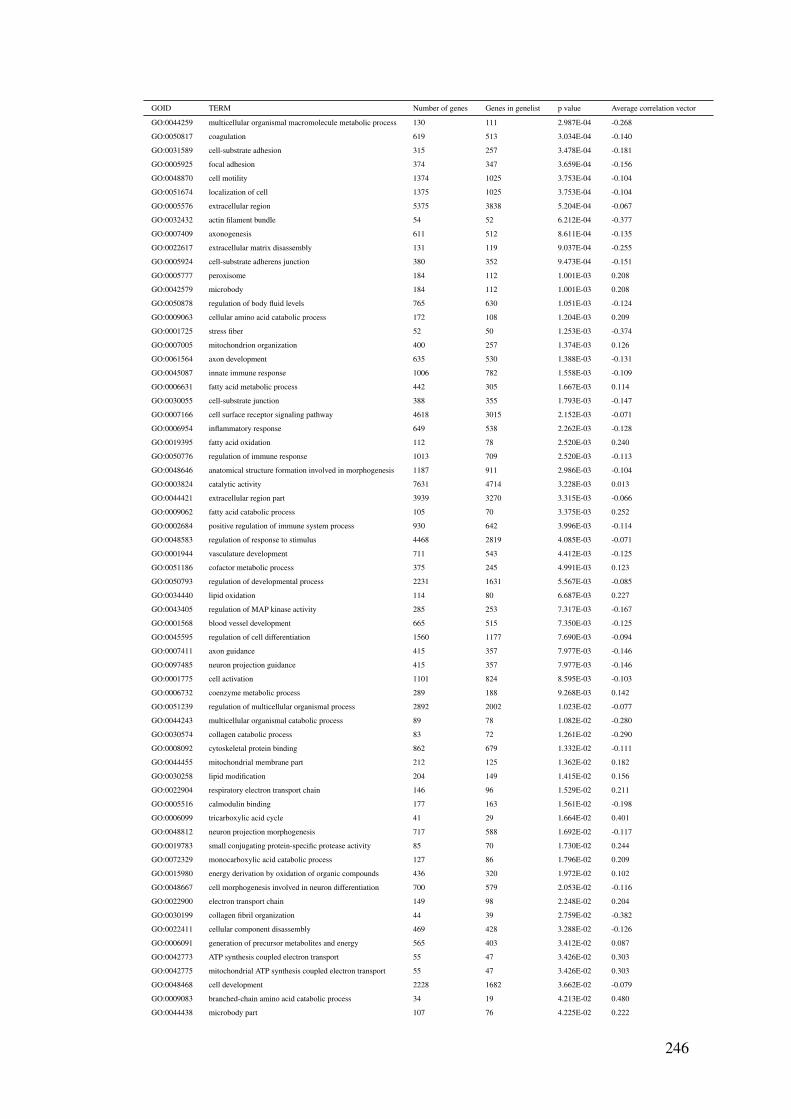
GOID TERM Number of genes Genes in genelist p value Average correlation vector
GO:0044259 multicellular organismal macromolecule metabolic process 130 111 2.987E-04 -0.268
GO:0050817 coagulation 619 513 3.034E-04 -0.140
GO:0031589 cell-substrate adhesion 315 257 3.478E-04 -0.181
GO:0005925 focal adhesion 374 347 3.659E-04 -0.156
GO:0048870 cell motility 1374 1025 3.753E-04 -0.104
GO:0051674 localization of cell 1375 1025 3.753E-04 -0.104
GO:0005576 extracellular region 5375 3838 5.204E-04 -0.067
GO:0032432 actin filament bundle 54 52 6.212E-04 -0.377
GO:0007409 axonogenesis 611 512 8.611E-04 -0.135
GO:0022617 extracellular matrix disassembly 131 119 9.037E-04 -0.255
GO:0005924 cell-substrate adherens junction 380 352 9.473E-04 -0.151
GO:0005777 peroxisome 184 112 1.001E-03 0.208
GO:0042579 microbody 184 112 1.001E-03 0.208
GO:0050878 regulation of body fluid levels 765 630 1.051E-03 -0.124
GO:0009063 cellular amino acid catabolic process 172 108 1.204E-03 0.209
GO:0001725 stress fiber 52 50 1.253E-03 -0.374
GO:0007005 mitochondrion organization 400 257 1.374E-03 0.126
GO:0061564 axon development 635 530 1.388E-03 -0.131
GO:0045087 innate immune response 1006 782 1.558E-03 -0.109
GO:0006631 fatty acid metabolic process 442 305 1.667E-03 0.114
GO:0030055 cell-substrate junction 388 355 1.793E-03 -0.147
GO:0007166 cell surface receptor signaling pathway 4618 3015 2.152E-03 -0.071
GO:0006954 inflammatory response 649 538 2.262E-03 -0.128
GO:0019395 fatty acid oxidation 112 78 2.520E-03 0.240
GO:0050776 regulation of immune response 1013 709 2.520E-03 -0.113
GO:0048646 anatomical structure formation involved in morphogenesis 1187 911 2.986E-03 -0.104
GO:0003824 catalytic activity 7631 4714 3.228E-03 0.013
GO:0044421 extracellular region part 3939 3270 3.315E-03 -0.066
GO:0009062 fatty acid catabolic process 105 70 3.375E-03 0.252
GO:0002684 positive regulation of immune system process 930 642 3.996E-03 -0.114
GO:0048583 regulation of response to stimulus 4468 2819 4.085E-03 -0.071
GO:0001944 vasculature development 711 543 4.412E-03 -0.125
GO:0051186 cofactor metabolic process 375 245 4.991E-03 0.123
GO:0050793 regulation of developmental process 2231 1631 5.567E-03 -0.085
GO:0034440 lipid oxidation 114 80 6.687E-03 0.227
GO:0043405 regulation of MAP kinase activity 285 253 7.317E-03 -0.167
GO:0001568 blood vessel development 665 515 7.350E-03 -0.125
GO:0045595 regulation of cell differentiation 1560 1177 7.690E-03 -0.094
GO:0007411 axon guidance 415 357 7.977E-03 -0.146
GO:0097485 neuron projection guidance 415 357 7.977E-03 -0.146
GO:0001775 cell activation 1101 824 8.595E-03 -0.103
GO:0006732 coenzyme metabolic process 289 188 9.268E-03 0.142
GO:0051239 regulation of multicellular organismal process 2892 2002 1.023E-02 -0.077
GO:0044243 multicellular organismal catabolic process 89 78 1.082E-02 -0.280
GO:0030574 collagen catabolic process 83 72 1.261E-02 -0.290
GO:0008092 cytoskeletal protein binding 862 679 1.332E-02 -0.111
GO:0044455 mitochondrial membrane part 212 125 1.362E-02 0.182
GO:0030258 lipid modification 204 149 1.415E-02 0.156
GO:0022904 respiratory electron transport chain 146 96 1.529E-02 0.211
GO:0005516 calmodulin binding 177 163 1.561E-02 -0.198
GO:0006099 tricarboxylic acid cycle 41 29 1.664E-02 0.401
GO:0048812 neuron projection morphogenesis 717 588 1.692E-02 -0.117
GO:0019783 small conjugating protein-specific protease activity 85 70 1.730E-02 0.244
GO:0072329 monocarboxylic acid catabolic process 127 86 1.796E-02 0.209
GO:0015980 energy derivation by oxidation of organic compounds 436 320 1.972E-02 0.102
GO:0048667 cell morphogenesis involved in neuron differentiation 700 579 2.053E-02 -0.116
GO:0022900 electron transport chain 149 98 2.248E-02 0.204
GO:0030199 collagen fibril organization 44 39 2.759E-02 -0.382
GO:0022411 cellular component disassembly 469 428 3.288E-02 -0.126
GO:0006091 generation of precursor metabolites and energy 565 403 3.412E-02 0.087
GO:0042773 ATP synthesis coupled electron transport 55 47 3.426E-02 0.303
GO:0042775 mitochondrial ATP synthesis coupled electron transport 55 47 3.426E-02 0.303
GO:0048468 cell development 2228 1682 3.662E-02 -0.079
GO:0009083 branched-chain amino acid catabolic process 34 19 4.213E-02 0.480
GO:0044438 microbody part 107 76 4.225E-02 0.222
246

GOID TERM Number of genes Genes in genelist p value Average correlation vector
GO:0044439 peroxisomal part 107 76 4.225E-02 0.222
GO:0010812 negative regulation of cell-substrate adhesion 44 37 4.459E-02 -0.363
GO:0004872 receptor activity 1940 1421 4.819E-02 -0.082
GO:0034097 response to cytokine 752 572 4.841E-02 -0.110
GO:0016790 thiolester hydrolase activity 79 58 4.918E-02 0.247
Table B.9: Gene set enrichment results of average correlation vector for biclustering patternMito.CV1 found in CCLE analysis in Section 3.3.3.2, showing the top 200 of 1219significant terms with adjusted p value < 0.05.
GOID TERM Number of genes Genes in genelist p value Average correlation vector
GO:0005739 mitochondrion 2109 1334 7.077E-32 0.141
GO:0044429 mitochondrial part 1081 711 4.360E-23 0.169
GO:0005759 mitochondrial matrix 365 300 4.700E-18 0.241
GO:0030198 extracellular matrix organization 422 357 3.513E-09 -0.207
GO:0043062 extracellular structure organization 424 358 3.877E-09 -0.207
GO:0003779 actin binding 402 350 7.029E-09 -0.206
GO:0005740 mitochondrial envelope 743 482 1.514E-08 0.129
GO:0055114 oxidation-reduction process 1187 905 6.836E-08 0.084
GO:0006935 chemotaxis 799 606 1.089E-07 -0.150
GO:0042330 taxis 799 606 1.089E-07 -0.150
GO:0031012 extracellular matrix 558 390 1.541E-07 -0.187
GO:0009653 anatomical structure morphogenesis 3188 2160 1.649E-07 -0.094
GO:0031967 organelle envelope 1166 778 1.746E-07 0.090
GO:0006955 immune response 1821 1241 2.454E-07 -0.111
GO:0031966 mitochondrial membrane 689 451 2.649E-07 0.124
GO:0006928 cellular component movement 2080 1488 3.695E-07 -0.105
GO:0048037 cofactor binding 274 236 3.811E-07 0.178
GO:0031975 envelope 1172 782 5.317E-07 0.088
GO:0040011 locomotion 1887 1350 7.393E-07 -0.107
GO:0022610 biological adhesion 1342 999 1.006E-06 -0.122
GO:0007155 cell adhesion 1334 995 1.116E-06 -0.122
GO:0050662 coenzyme binding 191 168 1.131E-06 0.212
GO:0019752 carboxylic acid metabolic process 1430 905 1.748E-06 0.074
GO:0016054 organic acid catabolic process 304 196 1.806E-06 0.184
GO:0046395 carboxylic acid catabolic process 304 196 1.806E-06 0.184
GO:0002376 immune system process 3353 2069 1.861E-06 -0.089
GO:0005743 mitochondrial inner membrane 488 310 2.972E-06 0.149
GO:0044282 small molecule catabolic process 371 255 4.350E-06 0.156
GO:0000904 cell morphogenesis involved in differentiation 954 757 4.857E-06 -0.130
GO:0006952 defense response 1956 1337 6.233E-06 -0.102
GO:0000902 cell morphogenesis 1341 1025 6.544E-06 -0.115
GO:0009611 response to wounding 1117 903 6.575E-06 -0.123
GO:0032989 cellular component morphogenesis 1428 1093 7.239E-06 -0.112
GO:0009605 response to external stimulus 2532 1822 1.135E-05 -0.091
GO:0042060 wound healing 781 640 1.267E-05 -0.138
GO:0015629 actin cytoskeleton 462 365 1.603E-05 -0.172
GO:0045333 cellular respiration 221 148 3.650E-05 0.208
GO:0019866 organelle inner membrane 531 345 3.863E-05 0.127
GO:0030036 actin cytoskeleton organization 599 451 3.992E-05 -0.155
GO:0005615 extracellular space 1277 1103 4.095E-05 -0.110
GO:0043436 oxoacid metabolic process 1574 1012 4.874E-05 0.061
GO:0009060 aerobic respiration 60 46 5.733E-05 0.384
GO:0005578 proteinaceous extracellular matrix 365 320 6.081E-05 -0.178
GO:0007599 hemostasis 622 515 6.450E-05 -0.145
GO:0006082 organic acid metabolic process 1593 1026 7.265E-05 0.059
GO:0042641 actomyosin 63 58 9.342E-05 -0.380
GO:0016491 oxidoreductase activity 984 607 1.111E-04 0.086
GO:0007596 blood coagulation 615 510 1.122E-04 -0.144
GO:0030029 actin filament-based process 677 501 1.253E-04 -0.143
GO:1990204 oxidoreductase complex 123 76 1.493E-04 0.285
GO:0005518 collagen binding 65 60 1.507E-04 -0.359
GO:0032963 collagen metabolic process 124 105 1.743E-04 -0.280
247

GOID TERM Number of genes Genes in genelist p value Average correlation vector
GO:0002682 regulation of immune system process 1544 1054 2.054E-04 -0.104
GO:0016477 cell migration 1277 960 2.293E-04 -0.108
GO:0044259 multicellular organismal macromolecule metabolic process 130 111 2.987E-04 -0.268
GO:0050817 coagulation 619 513 3.034E-04 -0.140
GO:0031589 cell-substrate adhesion 315 257 3.478E-04 -0.181
GO:0005925 focal adhesion 374 347 3.659E-04 -0.156
GO:0048870 cell motility 1374 1025 3.753E-04 -0.104
GO:0051674 localization of cell 1375 1025 3.753E-04 -0.104
GO:0005576 extracellular region 5375 3838 5.204E-04 -0.067
GO:0032432 actin filament bundle 54 52 6.212E-04 -0.377
GO:0007409 axonogenesis 611 512 8.611E-04 -0.135
GO:0022617 extracellular matrix disassembly 131 119 9.037E-04 -0.255
GO:0005924 cell-substrate adherens junction 380 352 9.473E-04 -0.151
GO:0005777 peroxisome 184 112 1.001E-03 0.208
GO:0042579 microbody 184 112 1.001E-03 0.208
GO:0050878 regulation of body fluid levels 765 630 1.051E-03 -0.124
GO:0009063 cellular amino acid catabolic process 172 108 1.204E-03 0.209
GO:0001725 stress fiber 52 50 1.253E-03 -0.374
GO:0007005 mitochondrion organization 400 257 1.374E-03 0.126
GO:0061564 axon development 635 530 1.388E-03 -0.131
GO:0045087 innate immune response 1006 782 1.558E-03 -0.109
GO:0006631 fatty acid metabolic process 442 305 1.667E-03 0.114
GO:0030055 cell-substrate junction 388 355 1.793E-03 -0.147
GO:0007166 cell surface receptor signaling pathway 4618 3015 2.152E-03 -0.071
GO:0006954 inflammatory response 649 538 2.262E-03 -0.128
GO:0019395 fatty acid oxidation 112 78 2.520E-03 0.240
GO:0050776 regulation of immune response 1013 709 2.520E-03 -0.113
GO:0048646 anatomical structure formation involved in morphogenesis 1187 911 2.986E-03 -0.104
GO:0003824 catalytic activity 7631 4714 3.228E-03 0.013
GO:0044421 extracellular region part 3939 3270 3.315E-03 -0.066
GO:0009062 fatty acid catabolic process 105 70 3.375E-03 0.252
GO:0002684 positive regulation of immune system process 930 642 3.996E-03 -0.114
GO:0048583 regulation of response to stimulus 4468 2819 4.085E-03 -0.071
GO:0001944 vasculature development 711 543 4.412E-03 -0.125
GO:0051186 cofactor metabolic process 375 245 4.991E-03 0.123
GO:0050793 regulation of developmental process 2231 1631 5.567E-03 -0.085
GO:0034440 lipid oxidation 114 80 6.687E-03 0.227
GO:0043405 regulation of MAP kinase activity 285 253 7.317E-03 -0.167
GO:0001568 blood vessel development 665 515 7.350E-03 -0.125
GO:0045595 regulation of cell differentiation 1560 1177 7.690E-03 -0.094
GO:0007411 axon guidance 415 357 7.977E-03 -0.146
GO:0097485 neuron projection guidance 415 357 7.977E-03 -0.146
GO:0001775 cell activation 1101 824 8.595E-03 -0.103
GO:0006732 coenzyme metabolic process 289 188 9.268E-03 0.142
GO:0051239 regulation of multicellular organismal process 2892 2002 1.023E-02 -0.077
GO:0044243 multicellular organismal catabolic process 89 78 1.082E-02 -0.280
GO:0030574 collagen catabolic process 83 72 1.261E-02 -0.290
GO:0008092 cytoskeletal protein binding 862 679 1.332E-02 -0.111
GO:0044455 mitochondrial membrane part 212 125 1.362E-02 0.182
GO:0030258 lipid modification 204 149 1.415E-02 0.156
GO:0022904 respiratory electron transport chain 146 96 1.529E-02 0.211
GO:0005516 calmodulin binding 177 163 1.561E-02 -0.198
GO:0006099 tricarboxylic acid cycle 41 29 1.664E-02 0.401
GO:0048812 neuron projection morphogenesis 717 588 1.692E-02 -0.117
GO:0019783 small conjugating protein-specific protease activity 85 70 1.730E-02 0.244
GO:0072329 monocarboxylic acid catabolic process 127 86 1.796E-02 0.209
GO:0015980 energy derivation by oxidation of organic compounds 436 320 1.972E-02 0.102
GO:0048667 cell morphogenesis involved in neuron differentiation 700 579 2.053E-02 -0.116
GO:0022900 electron transport chain 149 98 2.248E-02 0.204
GO:0030199 collagen fibril organization 44 39 2.759E-02 -0.382
GO:0022411 cellular component disassembly 469 428 3.288E-02 -0.126
GO:0006091 generation of precursor metabolites and energy 565 403 3.412E-02 0.087
GO:0042773 ATP synthesis coupled electron transport 55 47 3.426E-02 0.303
GO:0042775 mitochondrial ATP synthesis coupled electron transport 55 47 3.426E-02 0.303
GO:0048468 cell development 2228 1682 3.662E-02 -0.079
248

GOID TERM Number of genes Genes in genelist p value Average correlation vector
GO:0009083 branched-chain amino acid catabolic process 34 19 4.213E-02 0.480
GO:0044438 microbody part 107 76 4.225E-02 0.222
GO:0044439 peroxisomal part 107 76 4.225E-02 0.222
GO:0010812 negative regulation of cell-substrate adhesion 44 37 4.459E-02 -0.363
GO:0004872 receptor activity 1940 1421 4.819E-02 -0.082
GO:0034097 response to cytokine 752 572 4.841E-02 -0.110
GO:0016790 thiolester hydrolase activity 79 58 4.918E-02 0.247
Table B.10: Gene set enrichment results of average correlation vector for biclustering patternRandom.CV1 found in CCLE analysis in Section 3.3.3.2, showing the top 200 of1061 significant terms with adjusted p value < 0.05.
GOID TERM Number of genes Genes in genelist p value Average correlation vector
GO:0003676 nucleic acid binding 4689 3350 2.586E-91 -0.133
GO:0090304 nucleic acid metabolic process 7863 4176 3.400E-77 -0.103
GO:0005576 extracellular region 5375 3798 8.376E-77 0.214
GO:0005634 nucleus 8112 5630 1.348E-72 -0.081
GO:0044421 extracellular region part 3939 3230 4.597E-69 0.217
GO:0003677 DNA binding 2781 2080 2.747E-67 -0.149
GO:0005654 nucleoplasm 1793 1352 7.682E-66 -0.183
GO:0031981 nuclear lumen 2785 1990 2.335E-65 -0.143
GO:0044428 nuclear part 3483 2343 6.489E-63 -0.125
GO:0016070 RNA metabolic process 6737 3690 1.874E-61 -0.095
GO:0006952 defense response 1956 1314 2.036E-55 0.270
GO:0005615 extracellular space 1277 1085 3.828E-54 0.290
GO:0006139 nucleobase-containing compound metabolic process 9873 5452 5.174E-54 -0.063
GO:0043230 extracellular organelle 2671 2413 1.369E-52 0.216
GO:0065010 extracellular membrane-bounded organelle 2671 2413 1.369E-52 0.216
GO:0070062 extracellular vesicular exosome 2669 2413 1.369E-52 0.216
GO:0051276 chromosome organization 1127 741 1.776E-52 -0.232
GO:1901363 heterocyclic compound binding 7008 5069 2.535E-52 -0.065
GO:0046483 heterocycle metabolic process 10158 5608 5.391E-49 -0.057
GO:0097159 organic cyclic compound binding 7093 5136 8.291E-49 -0.060
GO:0006725 cellular aromatic compound metabolic process 10189 5618 1.582E-48 -0.056
GO:0006955 immune response 1821 1235 3.003E-48 0.262
GO:0071944 cell periphery 6341 3965 9.122E-47 0.179
GO:0031982 vesicle 3913 3116 1.369E-46 0.191
GO:0005886 plasma membrane 6168 3876 2.998E-46 0.180
GO:0032774 RNA biosynthetic process 5516 3094 4.327E-46 -0.087
GO:0031224 intrinsic component of membrane 5833 4422 4.973E-46 0.174
GO:0044451 nucleoplasm part 717 589 6.541E-46 -0.241
GO:0044425 membrane part 7949 5245 6.728E-46 0.166
GO:0031988 membrane-bounded vesicle 3783 3029 6.980E-46 0.192
GO:0016021 integral component of membrane 5650 4318 2.911E-44 0.173
GO:0006351 transcription, DNA-templated 5382 3031 1.070E-43 -0.085
GO:0051252 regulation of RNA metabolic process 4486 3046 2.535E-43 -0.084
GO:0044459 plasma membrane part 2761 2039 3.088E-43 0.215
GO:0034641 cellular nitrogen compound metabolic process 10485 5809 4.265E-43 -0.049
GO:2000112 regulation of cellular macromolecule biosynthetic process 4707 3201 2.300E-42 -0.080
GO:0034654 nucleobase-containing compound biosynthetic process 6012 3404 3.820E-42 -0.075
GO:0010467 gene expression 7890 4342 5.898E-42 -0.061
GO:0019438 aromatic compound biosynthetic process 6127 3474 5.702E-41 -0.072
GO:0003723 RNA binding 1808 1346 6.125E-41 -0.132
GO:0018130 heterocycle biosynthetic process 6129 3468 1.287E-40 -0.072
GO:1901360 organic cyclic compound metabolic process 10552 5810 1.397E-40 -0.046
GO:0002376 immune system process 3353 2071 1.443E-40 0.206
GO:2001141 regulation of RNA biosynthetic process 4359 2971 4.417E-40 -0.081
GO:0006954 inflammatory response 649 529 9.354E-40 0.338
GO:0006355 regulation of transcription, DNA-templated 4286 2936 6.760E-39 -0.080
GO:0010556 regulation of macromolecule biosynthetic process 4909 3301 1.110E-38 -0.072
GO:0044271 cellular nitrogen compound biosynthetic process 6227 3521 1.862E-38 -0.068
GO:0006397 mRNA processing 610 383 2.044E-38 -0.282
GO:0006325 chromatin organization 853 558 2.265E-38 -0.229
249

GOID TERM Number of genes Genes in genelist p value Average correlation vector
GO:0006396 RNA processing 993 629 7.450E-38 -0.204
GO:0034645 cellular macromolecule biosynthetic process 7021 3948 8.405E-38 -0.061
GO:0008380 RNA splicing 525 313 1.369E-37 -0.312
GO:0016071 mRNA metabolic process 885 537 3.668E-37 -0.222
GO:0016568 chromatin modification 661 495 6.727E-37 -0.240
GO:0005694 chromosome 905 668 7.767E-37 -0.200
GO:0031326 regulation of cellular biosynthetic process 5114 3445 1.007E-36 -0.067
GO:0031226 intrinsic component of plasma membrane 1430 1244 1.695E-36 0.239
GO:1901362 organic cyclic compound biosynthetic process 6314 3582 2.399E-36 -0.064
GO:0000278 mitotic cell cycle 1169 838 3.330E-36 -0.168
GO:0044822 poly(A) RNA binding 1170 1019 1.047E-35 -0.146
GO:0006259 DNA metabolic process 1393 841 1.459E-35 -0.168
GO:0005887 integral component of plasma membrane 1359 1199 7.192E-35 0.238
GO:0043207 response to external biotic stimulus 839 606 1.129E-34 0.303
GO:0051707 response to other organism 839 606 1.129E-34 0.303
GO:0009605 response to external stimulus 2532 1801 1.405E-34 0.205
GO:0009889 regulation of biosynthetic process 5182 3483 4.059E-34 -0.062
GO:0044260 cellular macromolecule metabolic process 12514 6531 4.486E-34 -0.034
GO:0009059 macromolecule biosynthetic process 7259 4074 6.901E-34 -0.054
GO:0010468 regulation of gene expression 5356 3560 1.198E-33 -0.061
GO:0019219 regulation of nucleobase-containing compound metabolic
process
5589 3760 1.583E-33 -0.057
GO:0009607 response to biotic stimulus 877 635 1.680E-33 0.293
GO:0007049 cell cycle 2122 1445 2.440E-33 -0.111
GO:0006807 nitrogen compound metabolic process 11158 6162 1.196E-32 -0.034
GO:0022402 cell cycle process 1520 1076 1.046E-31 -0.131
GO:1903047 mitotic cell cycle process 966 728 1.186E-31 -0.169
GO:0002682 regulation of immune system process 1544 1051 2.697E-31 0.238
GO:0070013 intracellular organelle lumen 3486 2557 3.505E-31 -0.068
GO:0006281 DNA repair 578 378 3.530E-31 -0.254
GO:0051171 regulation of nitrogen compound metabolic process 5711 3845 1.508E-30 -0.052
GO:0000375 RNA splicing, via transesterification reactions 358 214 1.782E-30 -0.347
GO:0044427 chromosomal part 783 577 1.992E-30 -0.195
GO:0009611 response to wounding 1117 890 5.677E-30 0.251
GO:0004872 receptor activity 1940 1117 6.129E-30 0.233
GO:0000377 RNA splicing, via transesterification reactions with bulged
adenosine as nucleophile
349 209 6.728E-30 -0.349
GO:0000398 mRNA splicing, via spliceosome 349 209 6.728E-30 -0.349
GO:0009986 cell surface 703 605 3.137E-29 0.288
GO:0002252 immune effector process 751 539 1.368E-28 0.293
GO:0098589 membrane region 1607 1312 1.436E-28 0.215
GO:0002684 positive regulation of immune system process 930 639 4.430E-28 0.275
GO:0001816 cytokine production 708 509 6.881E-28 0.298
GO:0043233 organelle lumen 3548 2610 1.171E-27 -0.061
GO:0031974 membrane-enclosed lumen 3621 2666 2.884E-27 -0.059
GO:0098542 defense response to other organism 438 329 1.841E-26 0.347
GO:1903034 regulation of response to wounding 393 325 2.258E-26 0.356
GO:0045087 innate immune response 1006 768 3.003E-26 0.249
GO:0009617 response to bacterium 461 358 3.867E-26 0.338
GO:0030198 extracellular matrix organization 422 356 9.629E-26 0.341
GO:0043062 extracellular structure organization 424 357 2.068E-25 0.339
GO:0038023 signaling receptor activity 1651 917 2.731E-25 0.237
GO:0031347 regulation of defense response 640 489 4.230E-25 0.293
GO:0001817 regulation of cytokine production 630 452 6.830E-25 0.300
GO:0004871 signal transducer activity 1971 1205 6.832E-25 0.212
GO:0060089 molecular transducer activity 1971 1205 6.832E-25 0.212
GO:0044770 cell cycle phase transition 530 443 1.836E-24 -0.198
GO:0001775 cell activation 1101 819 2.015E-24 0.240
GO:0042221 response to chemical 5076 3106 2.219E-24 0.155
GO:0015630 microtubule cytoskeleton 1219 860 3.312E-24 -0.126
GO:0016020 membrane 13317 7238 4.326E-24 0.128
GO:0044772 mitotic cell cycle phase transition 518 434 7.779E-24 -0.197
GO:0004888 transmembrane signaling receptor activity 1508 817 8.924E-24 0.243
GO:0032101 regulation of response to external stimulus 686 547 1.543E-23 0.274
GO:0006996 organelle organization 3692 2468 1.918E-23 -0.056
250

GOID TERM Number of genes Genes in genelist p value Average correlation vector
GO:0044249 cellular biosynthetic process 8617 4844 1.721E-22 -0.028
GO:0030529 ribonucleoprotein complex 744 528 3.930E-22 -0.160
GO:0048584 positive regulation of response to stimulus 2005 1395 5.038E-22 0.191
GO:0005813 centrosome 435 374 5.513E-22 -0.205
GO:0050776 regulation of immune response 1013 703 3.270E-21 0.241
GO:0070887 cellular response to chemical stimulus 3061 2054 6.905E-21 0.166
GO:1901576 organic substance biosynthetic process 8804 4937 1.591E-20 -0.024
GO:0022610 biological adhesion 1342 987 3.722E-20 0.211
GO:1990234 transferase complex 618 514 6.334E-20 -0.157
GO:0005681 spliceosomal complex 164 135 7.516E-20 -0.356
GO:0007155 cell adhesion 1334 982 7.941E-20 0.210
GO:0006974 cellular response to DNA damage stimulus 982 643 1.690E-19 -0.138
GO:0005783 endoplasmic reticulum 1847 1297 1.841E-19 0.189
GO:0009058 biosynthetic process 8929 5007 2.818E-19 -0.022
GO:0006950 response to stress 4845 3075 3.665E-19 0.143
GO:0044432 endoplasmic reticulum part 1158 912 5.614E-19 0.212
GO:0005815 microtubule organizing center 586 489 7.047E-19 -0.158
GO:0016569 covalent chromatin modification 447 341 7.824E-19 -0.203
GO:0051240 positive regulation of multicellular organismal process 724 565 1.287E-18 0.252
GO:0016570 histone modification 439 336 1.552E-18 -0.203
GO:0050727 regulation of inflammatory response 264 226 1.720E-18 0.361
GO:0016604 nuclear body 339 300 1.827E-18 -0.217
GO:0007165 signal transduction 7988 4490 2.144E-18 0.131
GO:0007017 microtubule-based process 631 464 2.642E-18 -0.161
GO:0000226 microtubule cytoskeleton organization 393 309 4.032E-18 -0.207
GO:0080134 regulation of response to stress 1172 899 4.698E-18 0.207
GO:1902494 catalytic complex 927 750 5.044E-18 -0.112
GO:0032991 macromolecular complex 5558 3965 5.663E-18 -0.024
GO:0002697 regulation of immune effector process 302 247 8.161E-18 0.337
GO:0003682 chromatin binding 422 385 9.164E-18 -0.187
GO:0034097 response to cytokine 752 557 1.050E-17 0.243
GO:0050865 regulation of cell activation 492 392 1.275E-17 0.283
GO:0000323 lytic vacuole 533 425 3.674E-17 0.268
GO:0005764 lysosome 533 425 3.674E-17 0.268
GO:0010033 response to organic substance 3172 2199 3.838E-17 0.154
GO:0070161 anchoring junction 478 414 4.912E-17 0.276
GO:1902533 positive regulation of intracellular signal transduction 820 659 5.633E-17 0.226
GO:0071824 protein-DNA complex subunit organization 165 132 6.133E-17 -0.349
GO:0012505 endomembrane system 4489 3002 7.334E-17 0.140
GO:0007166 cell surface receptor signaling pathway 4618 2712 9.610E-17 0.146
GO:0043231 intracellular membrane-bounded organelle 14352 8936 1.285E-16 -0.002
GO:0098552 side of membrane 311 279 1.347E-16 0.319
GO:0031012 extracellular matrix 558 388 1.561E-16 0.281
GO:0005125 cytokine activity 226 188 2.059E-16 0.369
GO:0045321 leukocyte activation 812 606 2.456E-16 0.233
GO:0048583 regulation of response to stimulus 4468 2843 4.898E-16 0.141
GO:0043229 intracellular organelle 16594 9839 5.355E-16 0.000
GO:0005102 receptor binding 1689 1199 5.508E-16 0.183
GO:0031323 regulation of cellular metabolic process 7614 4869 6.578E-16 -0.017
GO:1902589 single-organism organelle organization 2350 1660 1.221E-15 -0.056
GO:0000228 nuclear chromosome 390 330 1.328E-15 -0.191
GO:0050778 positive regulation of immune response 652 454 1.348E-15 0.255
GO:0043228 non-membrane-bounded organelle 4369 3101 2.085E-15 -0.027
GO:0043232 intracellular non-membrane-bounded organelle 4369 3101 2.085E-15 -0.027
GO:0032993 protein-DNA complex 334 244 2.240E-15 -0.225
GO:0000775 chromosome, centromeric region 214 153 2.948E-15 -0.295
GO:0051241 negative regulation of multicellular organismal process 416 355 3.077E-15 0.279
GO:0002237 response to molecule of bacterial origin 265 233 3.108E-15 0.328
GO:0005912 adherens junction 457 397 3.234E-15 0.270
GO:0042393 histone binding 139 123 3.276E-15 -0.339
GO:0002694 regulation of leukocyte activation 460 363 3.762E-15 0.276
GO:0016477 cell migration 1277 962 4.067E-15 0.192
GO:0005126 cytokine receptor binding 285 207 5.074E-15 0.344
GO:0042060 wound healing 781 632 5.124E-15 0.224
GO:0050896 response to stimulus 13313 6725 7.172E-15 0.114
251

GOID TERM Number of genes Genes in genelist p value Average correlation vector
GO:0052547 regulation of peptidase activity 447 337 1.023E-14 0.280
GO:0042742 defense response to bacterium 193 146 1.142E-14 0.396
GO:0000280 nuclear division 606 474 1.260E-14 -0.138
GO:0006261 DNA-dependent DNA replication 161 121 1.324E-14 -0.328
GO:0005773 vacuole 606 476 1.459E-14 0.243
GO:0071345 cellular response to cytokine stimulus 631 464 1.515E-14 0.243
GO:0006310 DNA recombination 273 202 2.180E-14 -0.244
GO:0005819 spindle 287 242 2.327E-14 -0.214
GO:0050900 leukocyte migration 362 288 2.587E-14 0.296
GO:0044839 cell cycle G2/M phase transition 180 163 2.654E-14 -0.274
GO:0009897 external side of plasma membrane 224 205 3.090E-14 0.340
GO:0048870 cell motility 1374 1029 3.702E-14 0.185
GO:0051674 localization of cell 1375 1029 3.702E-14 0.185
GO:0016607 nuclear speck 176 168 3.946E-14 -0.265
GO:0009888 tissue development 2160 1550 4.102E-14 0.164
GO:0000086 G2/M transition of mitotic cell cycle 178 162 4.245E-14 -0.273
GO:0030055 cell-substrate junction 388 341 4.941E-14 0.279
GO:0043170 macromolecule metabolic process 14207 7340 5.292E-14 -0.002
GO:0052548 regulation of endopeptidase activity 422 320 5.296E-14 0.280
GO:0098588 bounding membrane of organelle 2558 1891 5.427E-14 0.153
GO:0019221 cytokine-mediated signaling pathway 475 359 5.961E-14 0.265
GO:0006260 DNA replication 388 290 6.136E-14 -0.189
Table B.11: Gene set enrichment results of average correlation vector for biclustering patternRandom.CV2 found in CCLE analysis in Section 3.3.3.2, showing the top 200 of1186 significant terms with adjusted p value < 0.05.
GOID TERM Number of genes Genes in genelist p value Average correlation vector
GO:0006396 RNA processing 993 629 2.736E-101 0.677
GO:0003723 RNA binding 1808 1346 1.029E-86 0.510
GO:0031981 nuclear lumen 2785 1990 4.893E-78 0.460
GO:0044428 nuclear part 3483 2343 4.125E-74 0.436
GO:0012505 endomembrane system 4489 3002 2.136E-73 0.018
GO:0044822 poly(A) RNA binding 1170 1019 2.236E-72 0.513
GO:0098588 bounding membrane of organelle 2558 1891 3.131E-71 -0.021
GO:0030529 ribonucleoprotein complex 744 528 7.328E-70 0.633
GO:0016071 mRNA metabolic process 885 537 8.385E-67 0.632
GO:0005654 nucleoplasm 1793 1352 2.545E-66 0.489
GO:0009653 anatomical structure morphogenesis 3188 2184 4.611E-62 0.010
GO:0006397 mRNA processing 610 383 2.102E-59 0.672
GO:0022613 ribonucleoprotein complex biogenesis 339 250 2.049E-56 0.746
GO:0008380 RNA splicing 525 313 1.027E-54 0.700
GO:0005794 Golgi apparatus 1552 1173 1.452E-54 -0.067
GO:0070013 intracellular organelle lumen 3486 2557 1.810E-53 0.394
GO:0031982 vesicle 3913 3116 2.202E-53 0.060
GO:0003676 nucleic acid binding 4689 3350 1.082E-51 0.393
GO:0031974 membrane-enclosed lumen 3621 2666 4.990E-51 0.388
GO:0031988 membrane-bounded vesicle 3783 3029 7.218E-51 0.061
GO:0034660 ncRNA metabolic process 400 299 2.431E-50 0.676
GO:0043233 organelle lumen 3548 2610 4.818E-50 0.387
GO:0005783 endoplasmic reticulum 1847 1297 8.794E-49 -0.021
GO:0044421 extracellular region part 3939 3230 2.804E-48 0.077
GO:0000375 RNA splicing, via transesterification reactions 358 214 2.907E-48 0.755
GO:0000377 RNA splicing, via transesterification reactions with bulged
adenosine as nucleophile
349 209 9.253E-48 0.760
GO:0000398 mRNA splicing, via spliceosome 349 209 9.253E-48 0.760
GO:0034470 ncRNA processing 259 212 2.037E-47 0.741
GO:0005912 adherens junction 457 397 4.136E-46 -0.282
GO:0070161 anchoring junction 478 414 5.306E-46 -0.268
GO:0043230 extracellular organelle 2671 2413 1.750E-45 0.048
GO:0065010 extracellular membrane-bounded organelle 2671 2413 1.750E-45 0.048
GO:0070062 extracellular vesicular exosome 2669 2413 1.750E-45 0.048
GO:0009888 tissue development 2160 1550 1.156E-44 0.026
252

GOID TERM Number of genes Genes in genelist p value Average correlation vector
GO:0005576 extracellular region 5375 3798 8.353E-44 0.106
GO:0044431 Golgi apparatus part 904 713 1.585E-43 -0.097
GO:0044432 endoplasmic reticulum part 1158 912 5.730E-43 -0.050
GO:0098589 membrane region 1607 1312 1.947E-42 0.009
GO:0005925 focal adhesion 374 333 3.549E-41 -0.316
GO:0005924 cell-substrate adherens junction 380 338 4.963E-41 -0.310
GO:0030055 cell-substrate junction 388 341 6.150E-41 -0.305
GO:0072358 cardiovascular system development 1116 818 1.184E-40 -0.061
GO:0072359 circulatory system development 1116 818 1.184E-40 -0.061
GO:0006928 cellular component movement 2080 1497 8.602E-40 0.022
GO:0030198 extracellular matrix organization 422 356 1.914E-39 -0.239
GO:0044451 nucleoplasm part 717 589 2.093E-39 0.530
GO:0043062 extracellular structure organization 424 357 2.793E-39 -0.237
GO:0006259 DNA metabolic process 1393 841 1.418E-38 0.480
GO:0000139 Golgi membrane 624 535 2.562E-38 -0.130
GO:0040011 locomotion 1887 1358 2.393E-37 0.017
GO:0000902 cell morphogenesis 1341 1054 3.490E-37 -0.023
GO:0042254 ribosome biogenesis 188 146 7.699E-37 0.764
GO:0032989 cellular component morphogenesis 1428 1121 1.077E-36 -0.013
GO:0044425 membrane part 7949 5245 1.920E-36 0.143
GO:0030054 cell junction 1167 980 8.074E-36 -0.025
GO:0048731 system development 5637 3653 1.064E-34 0.114
GO:0005681 spliceosomal complex 164 135 1.708E-34 0.784
GO:0016192 vesicle-mediated transport 1419 1037 1.768E-34 -0.013
GO:0031090 organelle membrane 3375 2427 2.279E-34 0.069
GO:0016477 cell migration 1277 962 3.163E-34 -0.017
GO:0009966 regulation of signal transduction 3216 2194 6.245E-34 0.067
GO:0030030 cell projection organization 1349 1040 1.469E-33 -0.002
GO:0005694 chromosome 905 668 1.482E-33 0.490
GO:0001944 vasculature development 711 543 2.272E-33 -0.106
GO:0051276 chromosome organization 1127 741 8.585E-33 0.498
GO:0022610 biological adhesion 1342 987 4.257E-32 0.011
GO:0007155 cell adhesion 1334 982 7.356E-32 0.011
GO:0048856 anatomical structure development 6783 4258 8.134E-32 0.126
GO:0090304 nucleic acid metabolic process 7863 4176 9.095E-32 0.353
GO:0000904 cell morphogenesis involved in differentiation 954 767 1.344E-31 -0.043
GO:0005789 endoplasmic reticulum membrane 948 761 1.454E-31 -0.030
GO:0023051 regulation of signaling 3620 2458 3.502E-31 0.086
GO:0048646 anatomical structure formation involved in morphogenesis 1187 925 4.486E-31 -0.004
GO:0010646 regulation of cell communication 3631 2464 5.333E-31 0.087
GO:0048870 cell motility 1374 1029 7.590E-31 0.005
GO:0051674 localization of cell 1375 1029 7.590E-31 0.005
GO:0042175 nuclear outer membrane-endoplasmic reticulum membrane
network
971 776 9.223E-31 -0.024
GO:0060429 epithelium development 1252 962 2.233E-30 0.020
GO:0048858 cell projection morphogenesis 913 737 2.346E-30 -0.035
GO:0032502 developmental process 7760 4766 3.216E-30 0.135
GO:0006281 DNA repair 578 378 3.401E-30 0.545
GO:0001568 blood vessel development 665 513 4.518E-30 -0.097
GO:0022603 regulation of anatomical structure morphogenesis 843 697 7.400E-30 -0.042
GO:0007399 nervous system development 2516 1842 7.996E-30 0.074
GO:0007275 multicellular organismal development 6429 4162 1.899E-29 0.132
GO:0044767 single-organism developmental process 7612 4719 1.927E-29 0.136
GO:2000145 regulation of cell motility 608 501 2.294E-29 -0.100
GO:0016020 membrane 13317 7238 2.381E-29 0.156
GO:0005840 ribosome 251 149 3.883E-29 0.723
GO:0007154 cell communication 9101 5048 6.223E-29 0.147
GO:0023052 signaling 8975 4978 9.935E-29 0.146
GO:0044700 single organism signaling 8975 4978 9.935E-29 0.146
GO:0022008 neurogenesis 1639 1245 9.968E-29 0.043
GO:0032990 cell part morphogenesis 933 756 1.028E-28 -0.025
GO:0051179 localization 7894 4603 1.870E-28 0.135
GO:0005730 nucleolus 728 644 3.123E-28 0.454
GO:0006364 rRNA processing 125 106 3.225E-28 0.769
GO:0007165 signal transduction 7988 4490 3.754E-28 0.139
253

GOID TERM Number of genes Genes in genelist p value Average correlation vector
GO:0009887 organ morphogenesis 1011 818 4.789E-28 -0.001
GO:0040012 regulation of locomotion 685 553 5.724E-28 -0.073
GO:0016072 rRNA metabolic process 134 111 6.422E-28 0.757
GO:0031224 intrinsic component of membrane 5833 4422 6.989E-28 0.156
GO:0030334 regulation of cell migration 576 478 9.076E-28 -0.100
GO:0016021 integral component of membrane 5650 4318 9.417E-28 0.155
GO:0051270 regulation of cellular component movement 691 567 7.752E-27 -0.064
GO:0031410 cytoplasmic vesicle 1290 988 1.373E-26 0.022
GO:0044427 chromosomal part 783 577 2.154E-26 0.477
GO:0048583 regulation of response to stimulus 4468 2843 2.683E-26 0.108
GO:0048699 generation of neurons 1536 1174 2.787E-26 0.047
GO:0007167 enzyme linked receptor protein signaling pathway 1306 935 3.134E-26 0.006
GO:0048468 cell development 2228 1700 3.996E-26 0.075
GO:0071944 cell periphery 6341 3965 1.683E-25 0.150
GO:0031012 extracellular matrix 558 388 3.578E-25 -0.105
GO:0001501 skeletal system development 515 424 3.855E-25 -0.099
GO:0048869 cellular developmental process 4670 3189 4.254E-25 0.122
GO:0048514 blood vessel morphogenesis 583 448 5.136E-25 -0.091
GO:0031175 neuron projection development 943 756 7.766E-25 -0.005
GO:0048729 tissue morphogenesis 606 510 9.554E-25 -0.052
GO:0030182 neuron differentiation 1394 1078 9.933E-25 0.048
GO:0048812 neuron projection morphogenesis 717 590 1.013E-24 -0.042
GO:0003735 structural constituent of ribosome 160 97 2.857E-24 0.778
GO:0061564 axon development 635 531 8.577E-24 -0.049
GO:0008104 protein localization 2180 1688 8.701E-24 0.070
GO:0005886 plasma membrane 6168 3876 1.235E-23 0.153
GO:0050793 regulation of developmental process 2231 1648 1.531E-23 0.079
GO:0048667 cell morphogenesis involved in neuron differentiation 700 582 1.635E-23 -0.036
GO:2000026 regulation of multicellular organismal development 1647 1256 1.708E-23 0.060
GO:0042995 cell projection 1718 1367 3.670E-23 0.077
GO:0006310 DNA recombination 273 202 3.855E-23 0.642
GO:0005773 vacuole 606 476 7.406E-23 -0.082
GO:0035556 intracellular signal transduction 2879 2032 1.103E-22 0.097
GO:0048666 neuron development 1092 872 1.117E-22 0.029
GO:0007409 axonogenesis 611 513 1.424E-22 -0.048
GO:0042221 response to chemical 5076 3106 1.789E-22 0.133
GO:0048513 organ development 3828 2685 2.166E-22 0.123
GO:0051239 regulation of multicellular organismal process 2892 2012 2.633E-22 0.104
GO:0030154 cell differentiation 4368 3012 3.017E-22 0.127
GO:0044707 single-multicellular organism process 9631 5534 4.419E-22 0.166
GO:0016023 cytoplasmic membrane-bounded vesicle 1184 908 6.986E-22 0.033
GO:0005615 extracellular space 1277 1085 1.409E-21 0.078
GO:0044437 vacuolar part 374 315 1.544E-21 -0.154
GO:0022618 ribonucleoprotein complex assembly 173 121 1.803E-21 0.720
GO:0070887 cellular response to chemical stimulus 3061 2054 3.843E-21 0.108
GO:1902531 regulation of intracellular signal transduction 1855 1356 5.247E-21 0.070
GO:0071826 ribonucleoprotein complex subunit organization 180 128 6.280E-21 0.698
GO:0002009 morphogenesis of an epithelium 476 405 8.542E-21 -0.062
GO:0007507 heart development 533 420 1.425E-20 -0.057
GO:0032501 multicellular organismal process 9979 5713 1.595E-20 0.170
GO:0009100 glycoprotein metabolic process 495 366 2.127E-20 -0.084
GO:0072001 renal system development 330 263 2.317E-20 -0.133
GO:0016604 nuclear body 339 300 3.636E-20 0.520
GO:0044391 ribosomal subunit 153 84 4.234E-20 0.781
GO:0006261 DNA-dependent DNA replication 161 121 4.636E-20 0.679
GO:0006401 RNA catabolic process 282 169 4.732E-20 0.631
GO:0001525 angiogenesis 464 367 5.082E-20 -0.091
GO:0071310 cellular response to organic substance 2362 1650 6.035E-20 0.092
GO:0035295 tube development 675 566 6.377E-20 -0.011
GO:0030029 actin filament-based process 677 508 6.400E-20 -0.036
GO:0010033 response to organic substance 3172 2199 9.571E-20 0.113
GO:0071013 catalytic step 2 spliceosome 80 75 1.008E-19 0.808
GO:0006260 DNA replication 388 290 1.401E-19 0.510
GO:0001655 urogenital system development 373 300 1.929E-19 -0.102
GO:0005578 proteinaceous extracellular matrix 365 316 2.273E-19 -0.091
254

GOID TERM Number of genes Genes in genelist p value Average correlation vector
GO:0000323 lytic vacuole 533 425 4.422E-19 -0.078
GO:0005764 lysosome 533 425 4.422E-19 -0.078
GO:0033036 macromolecule localization 2639 1976 4.498E-19 0.095
GO:0016070 RNA metabolic process 6737 3690 5.286E-19 0.335
GO:0030036 actin cytoskeleton organization 599 457 6.984E-19 -0.050
GO:0061061 muscle structure development 629 479 7.464E-19 -0.028
GO:1901363 heterocyclic compound binding 7008 5069 7.506E-19 0.324
GO:0045184 establishment of protein localization 1692 1342 8.596E-19 0.069
GO:0005634 nucleus 8112 5630 1.200E-18 0.314
GO:0015031 protein transport 1553 1242 2.700E-18 0.065
GO:0044444 cytoplasmic part 10781 6514 2.868E-18 0.151
GO:0001822 kidney development 309 248 3.429E-18 -0.119
GO:0097159 organic cyclic compound binding 7093 5136 3.549E-18 0.323
GO:0006974 cellular response to DNA damage stimulus 982 643 6.602E-18 0.421
GO:0048193 Golgi vesicle transport 241 198 7.141E-18 -0.184
GO:0010647 positive regulation of cell communication 1360 1065 7.398E-18 0.058
GO:0023057 negative regulation of signaling 1127 867 8.309E-18 0.029
GO:0034330 cell junction organization 262 217 9.561E-18 -0.147
GO:0005768 endosome 818 600 9.986E-18 -0.006
GO:0010648 negative regulation of cell communication 1129 869 1.150E-17 0.030
GO:0009611 response to wounding 1117 890 1.222E-17 0.058
GO:0048598 embryonic morphogenesis 650 536 1.258E-17 0.003
GO:0023056 positive regulation of signaling 1355 1060 1.329E-17 0.059
GO:0006810 transport 6295 3693 1.406E-17 0.151
GO:0070848 response to growth factor 843 648 1.529E-17 0.014
GO:0031589 cell-substrate adhesion 315 260 1.745E-17 -0.133
GO:0044765 single-organism transport 5155 3114 1.775E-17 0.148
GO:0007411 axon guidance 415 353 1.930E-17 -0.069
GO:0097485 neuron projection guidance 415 353 1.930E-17 -0.069
GO:0050673 epithelial cell proliferation 325 283 2.342E-17 -0.089
GO:0071363 cellular response to growth factor stimulus 822 632 2.576E-17 0.011
GO:0000228 nuclear chromosome 390 330 2.823E-17 0.506
GO:0051234 establishment of localization 6434 3778 3.016E-17 0.152
GO:0009968 negative regulation of signal transduction 1081 826 3.047E-17 0.025
GO:0032879 regulation of localization 2401 1757 4.952E-17 0.113
GO:0031252 cell leading edge 336 292 6.938E-17 -0.126
GO:0000278 mitotic cell cycle 1169 838 7.755E-17 0.389
Table B.12: Top 200 of 651 significant terms for ICT1 related gene set from Section 4.2.1calculated by gprofiler
TERM ID TERM Term size Overlap size p value
GO:0044446 intracellular organelle part 7885 545 1.090E-39
GO:0044422 organelle part 8104 550 1.180E-37
TF:M00803 1 Factor: E2F; motif: GGCGSG; match class: 1 14302 699 7.990E-35
GO:0031974 membrane-enclosed lumen 4250 351 5.570E-34
TF:M00716 1 Factor: ZF5; motif: GSGCGCGR; match class: 1 16480 760 2.450E-33
TF:M00803 0 Factor: E2F; motif: GGCGSG; match class: 0 17619 787 1.950E-31
GO:0070013 intracellular organelle lumen 4140 337 1.000E-30
GO:0044424 intracellular part 13685 751 4.730E-30
GO:0043233 organelle lumen 4194 338 5.930E-30
GO:0043229 intracellular organelle 11855 684 2.580E-29
GO:0043231 intracellular membrane-bounded organelle 10791 636 9.680E-27
GO:0005622 intracellular 14067 755 8.220E-26
GO:0043227 membrane-bounded organelle 11947 678 1.780E-25
GO:0043226 organelle 12901 713 2.960E-25
GO:0000786 nucleosome 106 41 9.780E-25
GO:0044815 DNA packaging complex 112 41 1.270E-23
TF:M00716 0 Factor: ZF5; motif: GSGCGCGR; match class: 0 19516 819 5.540E-23
GO:0006996 organelle organization 3711 293 6.290E-23
GO:0044429 mitochondrial part 967 122 7.600E-23
GO:0032991 macromolecular complex 4503 335 9.550E-23
GO:0043228 non-membrane-bounded organelle 3828 298 2.000E-22
255

TERM ID TERM Term size Overlap size p value
GO:0043232 intracellular non-membrane-bounded organelle 3828 298 2.000E-22
GO:0005743 mitochondrial inner membrane 496 82 5.510E-22
GO:0031981 nuclear lumen 3435 275 6.130E-22
REAC:2299718 Condensation of Prophase Chromosomes 72 34 3.110E-21
REAC:5334118 DNA methylation 63 32 3.660E-21
GO:0044428 nuclear part 3773 290 1.130E-20
GO:0071840 cellular component organization or biogenesis 6327 420 1.420E-20
REAC:73728 RNA Polymerase I Promoter Opening 61 31 1.840E-20
GO:0006414 translational elongation 219 52 2.090E-20
GO:0019866 organelle inner membrane 551 83 1.600E-19
TF:M04687 1 Factor: BRCA1; motif: TMTCGCGAG; match class: 1 19299 807 2.030E-19
GO:0006415 translational termination 179 46 2.480E-19
TF:M04710 1 Factor: CHD2; motif: TCTCGCGAG; match class: 1 19229 805 2.590E-19
GO:0005739 mitochondrion 1699 165 3.050E-19
REAC:912446 Meiotic recombination 86 35 3.170E-19
REAC:5625886 Activated PKN1 stimulates transcription of AR (androgen
receptor) regulated genes KLK2 and KLK3
66 31 3.870E-19
REAC:427359 SIRT1 negatively regulates rRNA Expression 66 31 3.870E-19
REAC:212300 PRC2 methylates histones and DNA 71 32 4.140E-19
GO:0005740 mitochondrial envelope 720 96 5.010E-19
TF:M01240 1 Factor: BEN; motif: CAGCGRNV; match class: 1 19940 822 5.350E-19
TF:M04703 1 Factor: c-ets-1; motif: TCTCGCGAG; match class: 1 19373 808 5.530E-19
TF:M02065 1 Factor: ER81; motif: RCCGGAARYN; match class: 1 12310 590 5.910E-19
REAC:73777 RNA Polymerase I Chain Elongation 88 35 7.910E-19
REAC:3214815 HDACs deacetylate histones 94 36 9.550E-19
GO:0032993 protein-DNA complex 169 44 1.210E-18
GO:0016043 cellular component organization 6199 407 1.730E-18
TF:M04760 1 Factor: GR; motif: TCTCGCGAG; match class: 1 18786 791 3.310E-18
REAC:427413 NoRC negatively regulates rRNA expression 104 37 5.190E-18
TF:M07250 0 Factor: E2F1; motif: NNNSSCGCSAANN; match class: 0 15286 686 8.940E-18
TF:M02065 0 Factor: ER81; motif: RCCGGAARYN; match class: 0 18422 780 9.590E-18
TF:M00025 0 Factor: Elk-1; motif: NNNNCCGGAARTNN; match class:
0
16217 715 1.130E-17
REAC:5250941 Negative epigenetic regulation of rRNA expression 107 37 1.610E-17
GO:0031966 mitochondrial membrane 679 90 1.750E-17
GO:0071822 protein complex subunit organization 1879 172 1.820E-17
GO:0043933 macromolecular complex subunit organization 2636 217 2.140E-17
GO:0005840 ribosome 235 50 2.730E-17
TF:M00196 0 Factor: Sp1; motif: NGGGGGCGGGGYN; match class: 0 15939 704 6.920E-17
REAC:5625740 RHO GTPases activate PKNs 93 34 7.270E-17
REAC:977225 Amyloid fiber formation 99 35 7.480E-17
KEGG:05322 Systemic lupus erythematosus 132 39 9.410E-17
GO:0000790 nuclear chromatin 291 55 1.090E-16
TF:M00695 0 Factor: ETF; motif: GVGGMGG; match class: 0 12819 600 1.150E-16
GO:0006413 translational initiation 273 53 1.510E-16
REAC:5250913 Positive epigenetic regulation of rRNA expression 89 33 1.510E-16
REAC:5250924 B-WICH complex positively regulates rRNA expression 89 33 1.510E-16
REAC:2559582 Senescence-Associated Secretory Phenotype (SASP) 108 36 2.130E-16
GO:0070125 mitochondrial translational elongation 84 30 2.350E-16
REAC:212165 Epigenetic regulation of gene expression 136 40 3.660E-16
TF:M01660 1 Factor: GABPalpha; motif: CTTCCK; match class: 1 9803 489 4.170E-16
GO:0044238 primary metabolic process 10482 591 5.050E-16
TF:M00025 1 Factor: Elk-1; motif: NNNNCCGGAARTNN; match class:
1
9525 478 5.740E-16
TF:M00333 0 Factor: ZF5; motif: NRNGNGCGCGCWN; match class: 0 16969 733 6.020E-16
GO:0044260 cellular macromolecule metabolic process 8596 509 6.970E-16
GO:0071704 organic substance metabolic process 10808 604 7.450E-16
GO:0008152 metabolic process 12055 654 1.090E-15
GO:0005737 cytoplasm 10606 595 1.110E-15
REAC:73854 RNA Polymerase I Promoter Clearance 107 35 1.330E-15
TF:M01660 0 Factor: GABPalpha; motif: CTTCCK; match class: 0 16709 724 1.380E-15
REAC:201722 Formation of the beta-catenin:TCF transactivating complex 89 32 1.550E-15
REAC:2559580 Oxidative Stress Induced Senescence 121 37 1.820E-15
GO:0032543 mitochondrial translation 118 34 1.970E-15
GO:0000785 chromatin 442 67 2.050E-15
256

TERM ID TERM Term size Overlap size p value
GO:0044237 cellular metabolic process 10390 585 2.060E-15
REAC:73864 RNA Polymerase I Transcription 109 35 2.610E-15
GO:0000228 nuclear chromosome 494 71 3.580E-15
REAC:1500620 Meiosis 117 36 4.170E-15
REAC:5578749 Transcriptional regulation by small RNAs 104 34 4.180E-15
GO:0034641 cellular nitrogen compound metabolic process 6616 415 4.490E-15
GO:0044391 ribosomal subunit 162 39 5.530E-15
TF:M04760 0 Factor: GR; motif: TCTCGCGAG; match class: 0 20652 831 1.020E-14
REAC:5619507 Activation of HOX genes during differentiation 121 36 1.420E-14
REAC:5617472 Activation of anterior HOX genes in hindbrain development
during early embryogenesis
121 36 1.420E-14
GO:0044454 nuclear chromosome part 460 67 1.740E-14
GO:0003735 structural constituent of ribosome 223 45 2.140E-14
GO:0043624 cellular protein complex disassembly 285 51 2.960E-14
REAC:2559583 Cellular Senescence 191 45 3.080E-14
GO:0070124 mitochondrial translational initiation 84 28 3.310E-14
GO:0000788 nuclear nucleosome 43 21 3.430E-14
GO:0006807 nitrogen compound metabolic process 6922 426 3.730E-14
GO:0003723 RNA binding 1598 146 3.780E-14
GO:0043170 macromolecule metabolic process 9286 533 3.820E-14
REAC:5389840 Mitochondrial translation elongation 86 30 4.730E-14
KEGG:05034 Alcoholism 180 42 5.500E-14
TF:M02052 0 Factor: EHF; motif: CSCGGAARTN; match class: 0 15733 688 6.270E-14
GO:0070126 mitochondrial translational termination 86 28 6.710E-14
TF:M02071 0 Factor: ETV7; motif: NCCGGAANNN; match class: 0 15243 672 6.760E-14
TF:M02070 1 Factor: TEL1; motif: CNCGGAANNN; match class: 1 9180 457 6.820E-14
TF:M00986 0 Factor: Churchill; motif: CGGGNN; match class: 0 18592 775 6.840E-14
GO:0044822 poly(A) RNA binding 1179 118 1.030E-13
REAC:68886 M Phase 302 57 1.050E-13
TF:M07395 0 Factor: Sp1; motif: NGGGGCGGGGN; match class: 0 14838 658 1.050E-13
REAC:171306 Packaging Of Telomere Ends 50 23 1.400E-13
GO:0007005 mitochondrion organization 765 89 1.450E-13
GO:0043241 protein complex disassembly 309 52 2.150E-13
TF:M07056 1 Factor: Pitx2; motif: WNTAAWCCCA; match class: 1 11975 558 2.470E-13
TF:M02114 1 Factor: pitx2; motif: NNTAAWCCCA; match class: 1 11975 558 2.470E-13
TF:M07052 0 Factor: NRF-1; motif: GCGCMTGCGCN; match class: 0 2876 190 3.460E-13
GO:0031967 organelle envelope 1109 112 3.820E-13
REAC:69278 Cell Cycle, Mitotic 482 74 3.830E-13
REAC:5368287 Mitochondrial translation 92 30 3.990E-13
TF:M02102 0 Factor: NRF-1; motif: YGCGCMTGCGC; match class: 0 4374 258 4.280E-13
TF:M02070 0 Factor: TEL1; motif: CNCGGAANNN; match class: 0 16235 701 5.020E-13
GO:0031975 envelope 1115 112 5.650E-13
REAC:201681 TCF dependent signaling in response to WNT 231 48 5.740E-13
GO:1990904 ribonucleoprotein complex 717 84 7.790E-13
GO:0030529 intracellular ribonucleoprotein complex 717 84 7.790E-13
GO:0006412 translation 677 81 8.220E-13
GO:1901363 heterocyclic compound binding 5944 374 9.440E-13
GO:0043043 peptide biosynthetic process 706 83 9.680E-13
GO:0032984 macromolecular complex disassembly 320 52 9.820E-13
GO:0006334 nucleosome assembly 144 34 1.610E-12
REAC:2559586 DNA Damage/Telomere Stress Induced Senescence 78 27 2.070E-12
TF:M04687 0 Factor: BRCA1; motif: TMTCGCGAG; match class: 0 21180 839 2.090E-12
TF:M02089 0 Factor: E2F-3; motif: GGCGGGN; match class: 0 16847 718 2.420E-12
REAC:211000 Gene Silencing by RNA 133 35 2.630E-12
GO:0010467 gene expression 5430 347 2.980E-12
REAC:5368286 Mitochondrial translation initiation 86 28 3.870E-12
REAC:5419276 Mitochondrial translation termination 86 28 3.870E-12
GO:0044427 chromosomal part 751 85 3.970E-12
GO:0044267 cellular protein metabolic process 5157 333 4.070E-12
REAC:195258 RHO GTPase Effectors 290 53 5.200E-12
GO:0044444 cytoplasmic part 8003 467 6.570E-12
TF:M07063 0 Factor: Sp1; motif: GGGGCGGGGC; match class: 0 14183 629 8.020E-12
TF:M07250 1 Factor: E2F1; motif: NNNSSCGCSAANN; match class: 1 9775 471 8.670E-12
GO:0097159 organic cyclic compound binding 6027 374 9.600E-12
257

TERM ID TERM Term size Overlap size p value
REAC:504046 RNA Polymerase I, RNA Polymerase III, and Mitochon-
drial Transcription
146 36 9.660E-12
REAC:68875 Mitotic Prophase 139 35 1.130E-11
TF:M04703 0 Factor: c-ets-1; motif: TCTCGCGAG; match class: 0 21372 842 1.180E-11
GO:0065004 protein-DNA complex assembly 193 38 1.840E-11
GO:0005654 nucleoplasm 2802 208 1.990E-11
TF:M00196 1 Factor: Sp1; motif: NGGGGGCGGGGYN; match class: 1 11615 537 2.360E-11
GO:0045814 negative regulation of gene expression, epigenetic 166 35 2.460E-11
GO:0005634 nucleus 6842 411 2.510E-11
GO:0044464 cell part 16166 791 2.580E-11
GO:0005759 mitochondrial matrix 405 57 2.580E-11
TF:M00931 0 Factor: Sp1; motif: GGGGCGGGGC; match class: 0 14606 641 3.110E-11
REAC:3214847 HATs acetylate histones 144 35 3.580E-11
REAC:392499 Metabolism of proteins 1065 118 4.230E-11
TF:M02067 0 Factor: ER71; motif: ACCGGAARYN; match class: 0 9257 448 5.400E-11
REAC:3214858 RMTs methylate histone arginines 75 25 5.850E-11
GO:0034728 nucleosome organization 171 35 6.350E-11
KEGG:03010 Ribosome 132 32 6.440E-11
GO:0031497 chromatin assembly 162 34 6.870E-11
GO:0003676 nucleic acid binding 4026 271 7.330E-11
TF:M03807 0 Factor: SP2; motif: GNNGGGGGCGGGGSN; match
class: 0
12009 549 7.670E-11
GO:0005623 cell 16203 791 7.810E-11
REAC:1640170 Cell Cycle 579 78 8.870E-11
REAC:774815 Nucleosome assembly 71 24 1.280E-10
REAC:606279 Deposition of new CENPA-containing nucleosomes at the
centromere
71 24 1.280E-10
TF:M03969 0 Factor: ELF5; motif: ANSMGGAAGTN; match class: 0 6745 348 1.280E-10
GO:0043604 amide biosynthetic process 784 84 1.350E-10
TF:M04710 0 Factor: CHD2; motif: TCTCGCGAG; match class: 0 21162 835 1.690E-10
TF:M00333 1 Factor: ZF5; motif: NRNGNGCGCGCWN; match class: 1 13100 586 1.880E-10
GO:0006333 chromatin assembly or disassembly 187 36 1.960E-10
GO:0005694 chromosome 848 88 2.050E-10
TF:M00428 0 Factor: E2F-1; motif: NKTSSCGC; match class: 0 8854 430 2.110E-10
REAC:157579 Telomere Maintenance 79 25 2.250E-10
GO:0006518 peptide metabolic process 835 87 2.280E-10
GO:0071824 protein-DNA complex subunit organization 220 39 2.930E-10
TF:M00932 0 Factor: Sp1; motif: NNGGGGCGGGGNN; match class: 0 14944 648 3.830E-10
TF:M07039 0 Factor: ETF; motif: CCCCGCCCCYN; match class: 0 14296 626 3.960E-10
GO:0043234 protein complex 3793 256 4.290E-10
GO:0006342 chromatin silencing 118 28 5.290E-10
REAC:1221632 Meiotic synapsis 76 24 6.960E-10
REAC:74160 Gene Expression 1411 140 7.180E-10
TF:M03924 0 Factor: YY1; motif: NNCGCCATTNN; match class: 0 7604 379 7.220E-10
GO:0000313 organellar ribosome 73 22 1.060E-09
GO:0005761 mitochondrial ribosome 73 22 1.060E-09
REAC:194315 Signaling by Rho GTPases 403 60 1.070E-09
TF:M07056 0 Factor: Pitx2; motif: WNTAAWCCCA; match class: 0 16403 694 1.310E-09
TF:M02114 0 Factor: pitx2; motif: NNTAAWCCCA; match class: 0 16403 694 1.310E-09
GO:0034622 cellular macromolecular complex assembly 923 91 1.460E-09
GO:0019538 protein metabolic process 5770 352 1.850E-09
TF:M02052 1 Factor: EHF; motif: CSCGGAARTN; match class: 1 8304 404 2.420E-09
TF:M02066 0 Factor: PEA3; motif: RCCGGAAGYN; match class: 0 5617 296 3.080E-09
REAC:69620 Cell Cycle Checkpoints 184 37 3.390E-09
REAC:195721 Signaling by Wnt 330 52 3.970E-09
GO:0043603 cellular amide metabolic process 1004 95 4.810E-09
TF:M02089 1 Factor: E2F-3; motif: GGCGGGN; match class: 1 12682 565 4.860E-09
258

Table B.13: Gene set enrichment results of average correlation vector for biclustering patternMito.CV1 found in breast cancer analysis in Section 4.2.3, showing the 120 signifi-cant terms with adjusted p value < 0.05.
GOID TERM Number of genes Genes in genelist p value Average correlation vector
GO:0098588 bounding membrane of organelle 2558 1770 5.991E-12 0.154
GO:0044444 cytoplasmic part 10781 6195 7.827E-12 0.109
GO:0044257 cellular protein catabolic process 614 451 1.868E-11 0.249
GO:0051603 proteolysis involved in cellular protein catabolic process 592 435 3.934E-11 0.250
GO:0031090 organelle membrane 3375 2291 5.007E-11 0.138
GO:0030163 protein catabolic process 762 560 1.303E-10 0.223
GO:0019941 modification-dependent protein catabolic process 542 400 6.791E-10 0.249
GO:0012505 endomembrane system 4489 2813 1.818E-09 0.126
GO:0006511 ubiquitin-dependent protein catabolic process 531 394 2.024E-09 0.246
GO:0043632 modification-dependent macromolecule catabolic process 546 404 3.683E-09 0.242
GO:0070647 protein modification by small protein conjugation or re-
moval
1004 678 4.421E-09 0.197
GO:0005768 endosome 818 567 6.512E-09 0.212
GO:0005739 mitochondrion 2109 1317 4.290E-08 0.150
GO:0005773 vacuole 606 455 1.133E-07 0.221
GO:0032446 protein modification by small protein conjugation 895 603 1.411E-07 0.195
GO:0043230 extracellular organelle 2671 2381 1.735E-07 0.123
GO:0065010 extracellular membrane-bounded organelle 2671 2381 1.735E-07 0.123
GO:0070062 extracellular vesicular exosome 2669 2381 1.735E-07 0.123
GO:0003824 catalytic activity 7631 4533 2.062E-07 0.104
GO:0016567 protein ubiquitination 817 567 2.370E-07 0.197
GO:0000323 lytic vacuole 533 410 2.973E-07 0.227
GO:0005764 lysosome 533 410 2.973E-07 0.227
GO:0048193 Golgi vesicle transport 241 189 6.386E-07 0.304
GO:0031982 vesicle 3913 3061 8.228E-07 0.113
GO:0031988 membrane-bounded vesicle 3783 2976 1.529E-06 0.113
GO:0044248 cellular catabolic process 3220 2183 1.653E-06 0.122
GO:0044267 cellular protein metabolic process 5601 3337 2.952E-06 0.108
GO:0006508 proteolysis 1615 1166 5.042E-06 0.147
GO:0044440 endosomal part 403 302 5.697E-06 0.239
GO:1902494 catalytic complex 927 695 1.109E-05 0.168
GO:0045184 establishment of protein localization 1692 1344 1.282E-05 0.137
GO:0005794 Golgi apparatus 1552 1103 1.640E-05 0.145
GO:0009056 catabolic process 3733 2523 1.959E-05 0.113
GO:0015031 protein transport 1553 1252 2.227E-05 0.139
GO:0005737 cytoplasm 14272 8228 3.492E-05 0.086
GO:0010498 proteasomal protein catabolic process 322 262 3.709E-05 0.240
GO:0004930 G-protein coupled receptor activity 987 646 7.246E-05 -0.079
GO:0010008 endosome membrane 394 294 8.631E-05 0.227
GO:0000786 nucleosome 67 54 9.704E-05 -0.393
GO:1990104 DNA bending complex 67 54 9.704E-05 -0.393
GO:0044815 DNA packaging complex 75 59 1.111E-04 -0.373
GO:0007264 small GTPase mediated signal transduction 567 453 1.152E-04 0.194
GO:0019001 guanyl nucleotide binding 409 334 1.273E-04 0.217
GO:0043565 sequence-specific DNA binding 829 661 1.339E-04 -0.079
GO:0005525 GTP binding 370 315 1.476E-04 0.220
GO:1901575 organic substance catabolic process 3412 2316 1.684E-04 0.111
GO:0032561 guanyl ribonucleotide binding 408 333 1.794E-04 0.215
GO:0008104 protein localization 2180 1666 2.433E-04 0.121
GO:0019003 GDP binding 48 47 3.496E-04 0.477
GO:0016787 hydrolase activity 3107 1999 4.395E-04 0.114
GO:0044437 vacuolar part 374 301 4.613E-04 0.217
GO:0016874 ligase activity 468 362 5.432E-04 0.199
GO:0044429 mitochondrial part 1081 707 5.514E-04 0.155
GO:0000209 protein polyubiquitination 199 178 5.902E-04 0.262
GO:0043161 proteasome-mediated ubiquitin-dependent protein catabolic
process
296 243 6.971E-04 0.230
GO:0003008 system process 2235 1570 7.992E-04 -0.031
GO:1990234 transferase complex 618 465 8.593E-04 0.177
GO:0006892 post-Golgi vesicle-mediated transport 99 86 9.056E-04 0.360
259

GOID TERM Number of genes Genes in genelist p value Average correlation vector
GO:0044431 Golgi apparatus part 904 664 1.091E-03 0.157
GO:0000139 Golgi membrane 624 493 1.533E-03 0.173
GO:0019538 protein metabolic process 7013 4073 1.552E-03 0.093
GO:0045335 phagocytic vesicle 98 71 1.585E-03 0.386
GO:0006505 GPI anchor metabolic process 51 30 1.909E-03 0.549
GO:0006464 cellular protein modification process 4196 2626 1.972E-03 0.102
GO:0036211 protein modification process 4196 2626 1.972E-03 0.102
GO:0007186 G-protein coupled receptor signaling pathway 1476 978 2.245E-03 -0.045
GO:0005777 peroxisome 184 107 2.383E-03 0.311
GO:0042579 microbody 184 107 2.383E-03 0.311
GO:0033036 macromolecule localization 2639 1933 3.108E-03 0.110
GO:1902582 single-organism intracellular transport 1497 1104 3.537E-03 0.128
GO:0045892 negative regulation of transcription, DNA-templated 1116 833 3.739E-03 -0.056
GO:0000977 RNA polymerase II regulatory region sequence-specific
DNA binding
301 264 3.830E-03 -0.128
GO:0044710 single-organism metabolic process 8623 4735 4.344E-03 0.089
GO:0006506 GPI anchor biosynthetic process 47 28 4.542E-03 0.548
GO:0030659 cytoplasmic vesicle membrane 426 354 4.580E-03 0.191
GO:0001012 RNA polymerase II regulatory region DNA binding 304 267 4.617E-03 -0.125
GO:0051340 regulation of ligase activity 115 104 4.721E-03 0.309
GO:0009083 branched-chain amino acid catabolic process 34 19 4.940E-03 0.657
GO:0006323 DNA packaging 164 116 5.143E-03 -0.217
GO:0051348 negative regulation of transferase activity 306 264 5.244E-03 0.214
GO:0009057 macromolecule catabolic process 1291 929 6.086E-03 0.132
GO:0043412 macromolecule modification 4389 2727 6.312E-03 0.099
GO:0000151 ubiquitin ligase complex 198 155 6.608E-03 0.255
GO:0000981 sequence-specific DNA binding RNA polymerase II tran-
scription factor activity
495 358 6.865E-03 -0.100
GO:0019882 antigen processing and presentation 258 215 7.266E-03 0.230
GO:0060271 cilium morphogenesis 187 130 7.453E-03 0.280
GO:0048002 antigen processing and presentation of peptide antigen 213 176 8.050E-03 0.247
GO:0012506 vesicle membrane 444 367 8.728E-03 0.185
GO:0044281 small molecule metabolic process 4814 2936 8.982E-03 0.097
GO:0031424 keratinization 49 43 9.515E-03 -0.369
GO:0051352 negative regulation of ligase activity 76 74 9.515E-03 0.349
GO:0051444 negative regulation of ubiquitin-protein transferase activity 76 74 9.515E-03 0.349
GO:0061024 membrane organization 927 729 9.528E-03 0.144
GO:0006661 phosphatidylinositol biosynthetic process 126 87 9.761E-03 0.321
GO:0007600 sensory perception 997 720 1.051E-02 -0.054
GO:0009081 branched-chain amino acid metabolic process 40 23 1.060E-02 0.588
GO:0043167 ion binding 6315 5058 1.117E-02 0.086
GO:0050877 neurological system process 1400 1033 1.168E-02 -0.038
GO:0005774 vacuolar membrane 299 235 1.418E-02 0.216
GO:1902679 negative regulation of RNA biosynthetic process 1142 850 1.496E-02 -0.049
GO:0002474 antigen processing and presentation of peptide antigen via
MHC class I
112 96 1.624E-02 0.309
GO:0044265 cellular macromolecule catabolic process 1040 740 1.624E-02 0.138
GO:0002478 antigen processing and presentation of exogenous peptide
antigen
176 161 1.760E-02 0.249
GO:0019884 antigen processing and presentation of exogenous antigen 178 163 1.785E-02 0.247
GO:0031396 regulation of protein ubiquitination 227 194 1.816E-02 0.227
GO:0005179 hormone activity 132 107 2.143E-02 -0.205
GO:0051436 negative regulation of ubiquitin-protein ligase activity in-
volved in mitotic cell cycle
68 67 2.589E-02 0.352
GO:0044712 single-organism catabolic process 2384 1667 2.674E-02 0.110
GO:0051253 negative regulation of RNA metabolic process 1174 872 3.028E-02 -0.045
GO:0016197 endosomal transport 217 157 3.081E-02 0.244
GO:0051351 positive regulation of ligase activity 96 88 3.098E-02 0.310
GO:0000122 negative regulation of transcription from RNA polymerase
II promoter
668 570 3.193E-02 -0.065
GO:0004888 transmembrane signaling receptor activity 1508 1000 3.233E-02 -0.034
GO:0006501 C-terminal protein lipidation 27 27 3.282E-02 0.517
GO:0071103 DNA conformation change 246 167 3.399E-02 -0.157
GO:0046907 intracellular transport 1822 1305 3.485E-02 0.115
GO:0051438 regulation of ubiquitin-protein transferase activity 110 99 3.522E-02 0.293
260

GOID TERM Number of genes Genes in genelist p value Average correlation vector
GO:0000976 transcription regulatory region sequence-specific DNA
binding
366 311 3.565E-02 -0.100
GO:0006664 glycolipid metabolic process 137 93 3.599E-02 0.304
GO:0044782 cilium organization 165 117 4.631E-02 0.272
Table B.14: Gene set enrichment results of average correlation vector for biclustering patternMito.CV2 found in breast cancer analysis in Section 4.2.3, showing the top 200 of443 significant terms with adjusted p value < 0.05.
GOID TERM Number of genes Genes in genelist p value Average correlation vector
GO:0003723 RNA binding 1808 1270 9.219E-32 -0.186
GO:0044428 nuclear part 3483 2183 5.253E-31 -0.150
GO:0000278 mitotic cell cycle 1169 781 1.476E-29 -0.229
GO:0031981 nuclear lumen 2785 1856 7.638E-29 -0.156
GO:0044822 poly(A) RNA binding 1170 964 8.930E-27 -0.195
GO:1903047 mitotic cell cycle process 966 674 1.021E-24 -0.226
GO:0034660 ncRNA metabolic process 400 274 7.249E-24 -0.324
GO:0070013 intracellular organelle lumen 3486 2415 1.579E-22 -0.128
GO:0031974 membrane-enclosed lumen 3621 2527 1.103E-21 -0.124
GO:0006259 DNA metabolic process 1393 778 2.784E-20 -0.193
GO:0043233 organelle lumen 3548 2472 6.835E-20 -0.121
GO:0005654 nucleoplasm 1793 1266 1.511E-19 -0.155
GO:0022402 cell cycle process 1520 1000 4.644E-18 -0.169
GO:0006396 RNA processing 993 548 5.761E-18 -0.210
GO:0006399 tRNA metabolic process 193 119 9.289E-18 -0.419
GO:0031012 extracellular matrix 558 386 1.045E-17 0.207
GO:0009653 anatomical structure morphogenesis 3188 2109 1.624E-17 0.079
GO:0044772 mitotic cell cycle phase transition 518 416 2.259E-17 -0.240
GO:0044770 cell cycle phase transition 530 427 1.017E-16 -0.234
GO:0030529 ribonucleoprotein complex 744 529 1.443E-15 -0.205
GO:0007049 cell cycle 2122 1355 4.754E-15 -0.140
GO:0034470 ncRNA processing 259 193 1.539E-14 -0.309
GO:0005578 proteinaceous extracellular matrix 365 316 1.561E-14 0.209
GO:0005739 mitochondrion 2109 1317 7.241E-14 -0.135
GO:0005730 nucleolus 728 585 3.128E-13 -0.184
GO:0005694 chromosome 905 627 3.599E-13 -0.179
GO:0008033 tRNA processing 106 77 3.918E-12 -0.440
GO:0044429 mitochondrial part 1081 707 4.048E-12 -0.165
GO:0000902 cell morphogenesis 1341 1011 6.741E-12 0.098
GO:0000793 condensed chromosome 200 149 9.314E-12 -0.336
GO:0072358 cardiovascular system development 1116 797 1.116E-11 0.110
GO:0072359 circulatory system development 1116 797 1.116E-11 0.110
GO:0007059 chromosome segregation 197 141 1.330E-11 -0.343
GO:0022613 ribonucleoprotein complex biogenesis 339 227 1.530E-11 -0.263
GO:0007167 enzyme linked receptor protein signaling pathway 1306 921 2.227E-11 0.102
GO:0000075 cell cycle checkpoint 275 224 2.597E-11 -0.271
GO:0022610 biological adhesion 1342 951 3.070E-11 0.099
GO:0006281 DNA repair 578 354 3.483E-11 -0.216
GO:0007155 cell adhesion 1334 947 3.831E-11 0.099
GO:0000082 G1/S transition of mitotic cell cycle 256 217 7.817E-11 -0.268
GO:0032989 cellular component morphogenesis 1428 1074 8.841E-11 0.090
GO:0032993 protein-DNA complex 334 239 1.140E-10 -0.256
GO:0048285 organelle fission 644 447 1.484E-10 -0.198
GO:0010646 regulation of cell communication 3631 2365 1.854E-10 0.056
GO:0023051 regulation of signaling 3620 2357 2.115E-10 0.056
GO:0001944 vasculature development 711 537 2.247E-10 0.131
GO:0000280 nuclear division 606 426 2.444E-10 -0.201
GO:0044843 cell cycle G1/S phase transition 259 219 2.765E-10 -0.262
GO:0007067 mitotic nuclear division 428 304 4.795E-10 -0.231
GO:0031967 organelle envelope 1166 770 4.838E-10 -0.147
GO:0031975 envelope 1172 774 4.926E-10 -0.147
GO:0030334 regulation of cell migration 576 474 6.727E-10 0.138
GO:0006974 cellular response to DNA damage stimulus 982 605 6.760E-10 -0.163
261

GOID TERM Number of genes Genes in genelist p value Average correlation vector
GO:0044427 chromosomal part 783 539 8.766E-10 -0.172
GO:0001568 blood vessel development 665 508 1.033E-09 0.131
GO:0005743 mitochondrial inner membrane 488 314 1.080E-09 -0.216
GO:0030030 cell projection organization 1349 996 1.104E-09 0.089
GO:0051270 regulation of cellular component movement 691 559 1.172E-09 0.125
GO:0071103 DNA conformation change 246 167 1.193E-09 -0.289
GO:0043228 non-membrane-bounded organelle 4369 2896 1.707E-09 -0.089
GO:0043232 intracellular non-membrane-bounded organelle 4369 2896 1.707E-09 -0.089
GO:0007389 pattern specification process 506 402 1.873E-09 0.146
GO:0019866 organelle inner membrane 531 347 1.963E-09 -0.204
GO:0031145 anaphase-promoting complex-dependent proteasomal
ubiquitin-dependent protein catabolic process
89 80 1.972E-09 -0.406
GO:0042254 ribosome biogenesis 188 138 2.023E-09 -0.305
GO:0001655 urogenital system development 373 292 2.390E-09 0.175
GO:2000145 regulation of cell motility 608 496 3.230E-09 0.130
GO:0046872 metal ion binding 4089 3375 5.902E-09 0.039
GO:0000313 organellar ribosome 60 49 6.311E-09 -0.489
GO:0005761 mitochondrial ribosome 60 49 6.311E-09 -0.489
GO:0000775 chromosome, centromeric region 214 139 7.045E-09 -0.313
GO:0006928 cellular component movement 2080 1457 7.608E-09 0.069
GO:0048646 anatomical structure formation involved in morphogenesis 1187 894 1.011E-08 0.089
GO:0043169 cation binding 4173 3440 1.014E-08 0.038
GO:0030198 extracellular matrix organization 422 352 1.068E-08 0.155
GO:0043062 extracellular structure organization 424 353 1.349E-08 0.154
GO:0048468 cell development 2228 1647 1.559E-08 0.062
GO:0009966 regulation of signal transduction 3216 2101 1.655E-08 0.054
GO:0048858 cell projection morphogenesis 913 711 1.828E-08 0.101
GO:0022603 regulation of anatomical structure morphogenesis 843 669 2.311E-08 0.105
GO:0016071 mRNA metabolic process 885 514 3.511E-08 -0.162
GO:0040012 regulation of locomotion 685 548 3.762E-08 0.116
GO:0006261 DNA-dependent DNA replication 161 106 3.896E-08 -0.335
GO:0044420 extracellular matrix part 147 117 4.034E-08 0.278
GO:0072001 renal system development 330 255 4.385E-08 0.175
GO:0042590 antigen processing and presentation of exogenous peptide
antigen via MHC class I
79 77 4.441E-08 -0.373
GO:2000026 regulation of multicellular organismal development 1647 1219 5.518E-08 0.072
GO:0048514 blood vessel morphogenesis 583 445 6.481E-08 0.128
GO:0009888 tissue development 2160 1526 6.621E-08 0.063
GO:0008380 RNA splicing 525 256 6.729E-08 -0.216
GO:0051239 regulation of multicellular organismal process 2892 1958 7.054E-08 0.053
GO:0032991 macromolecular complex 5558 3799 7.678E-08 -0.077
GO:0032990 cell part morphogenesis 933 728 8.632E-08 0.096
GO:0042995 cell projection 1718 1288 8.825E-08 0.068
GO:0006260 DNA replication 388 262 1.270E-07 -0.216
GO:0002479 antigen processing and presentation of exogenous peptide
antigen via MHC class I, TAP-dependent
75 73 1.294E-07 -0.375
GO:0003002 regionalization 375 312 1.412E-07 0.151
GO:0009123 nucleoside monophosphate metabolic process 624 466 1.470E-07 -0.166
GO:0000502 proteasome complex 127 64 1.726E-07 -0.406
GO:0006397 mRNA processing 610 322 1.907E-07 -0.189
GO:0009887 organ morphogenesis 1011 803 1.951E-07 0.090
GO:0007399 nervous system development 2516 1794 1.976E-07 0.055
GO:0000904 cell morphogenesis involved in differentiation 954 742 2.472E-07 0.093
GO:0001501 skeletal system development 515 417 2.506E-07 0.129
GO:0001822 kidney development 309 240 2.612E-07 0.174
GO:0051028 mRNA transport 143 102 2.885E-07 -0.313
GO:0050911 detection of chemical stimulus involved in sensory percep-
tion of smell
451 272 3.485E-07 -0.199
GO:0004984 olfactory receptor activity 418 272 3.485E-07 -0.199
GO:0051439 regulation of ubiquitin-protein ligase activity involved in mi-
totic cell cycle
81 75 3.661E-07 -0.374
GO:0000375 RNA splicing, via transesterification reactions 358 175 4.150E-07 -0.245
GO:0051436 negative regulation of ubiquitin-protein ligase activity in-
volved in mitotic cell cycle
68 67 4.230E-07 -0.392
GO:0048731 system development 5637 3561 4.687E-07 0.034
262

GOID TERM Number of genes Genes in genelist p value Average correlation vector
GO:0007275 multicellular organismal development 6429 4034 5.115E-07 0.031
GO:0006310 DNA recombination 273 185 5.259E-07 -0.245
GO:0040011 locomotion 1887 1323 6.062E-07 0.065
GO:0050793 regulation of developmental process 2231 1584 8.097E-07 0.056
GO:0000228 nuclear chromosome 390 308 8.327E-07 -0.192
GO:0007606 sensory perception of chemical stimulus 559 347 8.660E-07 -0.175
GO:0050907 detection of chemical stimulus involved in sensory percep-
tion
492 306 9.324E-07 -0.185
GO:0000377 RNA splicing, via transesterification reactions with bulged
adenosine as nucleophile
349 170 1.044E-06 -0.243
GO:0000398 mRNA splicing, via spliceosome 349 170 1.044E-06 -0.243
GO:0007093 mitotic cell cycle checkpoint 187 163 1.186E-06 -0.259
GO:1901990 regulation of mitotic cell cycle phase transition 280 234 1.198E-06 -0.218
GO:0016477 cell migration 1277 941 1.304E-06 0.078
GO:0005643 nuclear pore 78 59 1.374E-06 -0.396
GO:0000779 condensed chromosome, centromeric region 99 75 1.395E-06 -0.378
GO:0005740 mitochondrial envelope 743 483 1.429E-06 -0.156
GO:0009161 ribonucleoside monophosphate metabolic process 606 456 1.501E-06 -0.160
GO:0007169 transmembrane receptor protein tyrosine kinase signaling
pathway
873 653 1.568E-06 0.094
GO:0000819 sister chromatid segregation 73 55 1.706E-06 -0.429
GO:0044446 intracellular organelle part 9239 5593 1.710E-06 -0.067
GO:0072395 signal transduction involved in cell cycle checkpoint 72 67 2.157E-06 -0.377
GO:0051437 positive regulation of ubiquitin-protein ligase activity in-
volved in mitotic cell cycle
73 69 2.185E-06 -0.373
GO:0016779 nucleotidyltransferase activity 154 108 2.400E-06 -0.292
GO:0005524 ATP binding 1462 1285 2.496E-06 -0.106
GO:0005509 calcium ion binding 688 583 2.953E-06 0.099
GO:0007346 regulation of mitotic cell cycle 423 349 2.971E-06 -0.180
GO:0010564 regulation of cell cycle process 535 423 3.093E-06 -0.166
GO:0007608 sensory perception of smell 482 297 3.349E-06 -0.182
GO:0005759 mitochondrial matrix 365 296 3.491E-06 -0.192
GO:0030554 adenyl nucleotide binding 1525 1336 4.061E-06 -0.103
GO:0022008 neurogenesis 1639 1211 4.168E-06 0.063
GO:0031570 DNA integrity checkpoint 172 145 4.231E-06 -0.262
GO:0030182 neuron differentiation 1394 1045 4.293E-06 0.069
GO:0051301 cell division 890 638 4.596E-06 -0.142
GO:0048870 cell motility 1374 1002 4.879E-06 0.072
GO:0051674 localization of cell 1375 1002 4.879E-06 0.072
GO:0031397 negative regulation of protein ubiquitination 115 107 4.973E-06 -0.295
GO:0022616 DNA strand elongation 44 35 5.087E-06 -0.502
GO:0001525 angiogenesis 464 366 5.140E-06 0.127
GO:0072401 signal transduction involved in DNA integrity checkpoint 71 66 5.643E-06 -0.371
GO:0072413 signal transduction involved in mitotic cell cycle checkpoint 71 66 5.643E-06 -0.371
GO:0072422 signal transduction involved in DNA damage checkpoint 71 66 5.643E-06 -0.371
GO:1902402 signal transduction involved in mitotic DNA damage check-
point
71 66 5.643E-06 -0.371
GO:1902403 signal transduction involved in mitotic DNA integrity check-
point
71 66 5.643E-06 -0.371
GO:1901987 regulation of cell cycle phase transition 290 243 6.052E-06 -0.207
GO:0006271 DNA strand elongation involved in DNA replication 41 32 6.300E-06 -0.522
GO:0048699 generation of neurons 1536 1141 6.404E-06 0.064
GO:0031966 mitochondrial membrane 689 452 6.497E-06 -0.155
GO:0009126 purine nucleoside monophosphate metabolic process 591 444 7.125E-06 -0.156
GO:0032879 regulation of localization 2401 1726 7.141E-06 0.050
GO:0051352 negative regulation of ligase activity 76 74 8.376E-06 -0.350
GO:0051444 negative regulation of ubiquitin-protein transferase activity 76 74 8.376E-06 -0.350
GO:0050657 nucleic acid transport 171 120 8.665E-06 -0.267
GO:0050658 RNA transport 171 120 8.665E-06 -0.267
GO:0051236 establishment of RNA localization 171 120 8.665E-06 -0.267
GO:0009593 detection of chemical stimulus 527 338 9.366E-06 -0.168
GO:0006412 translation 771 462 9.393E-06 -0.153
GO:0007507 heart development 533 405 1.008E-05 0.115
GO:0009167 purine ribonucleoside monophosphate metabolic process 590 443 1.010E-05 -0.155
GO:0010648 negative regulation of cell communication 1129 849 1.056E-05 0.078
263

GOID TERM Number of genes Genes in genelist p value Average correlation vector
GO:0023057 negative regulation of signaling 1127 847 1.094E-05 0.078
GO:0000777 condensed chromosome kinetochore 90 70 1.180E-05 -0.370
GO:1903321 negative regulation of protein modification by small protein
conjugation or removal
121 112 1.210E-05 -0.283
GO:0006323 DNA packaging 164 116 1.307E-05 -0.283
GO:0046930 pore complex 95 75 1.330E-05 -0.330
GO:0072431 signal transduction involved in mitotic G1 DNA damage
checkpoint
69 65 1.421E-05 -0.365
GO:1902400 intracellular signal transduction involved in G1 DNA dam-
age checkpoint
69 65 1.421E-05 -0.365
GO:1902531 regulation of intracellular signal transduction 1855 1270 1.541E-05 0.060
GO:0044452 nucleolar part 39 32 1.614E-05 -0.507
GO:0000070 mitotic sister chromatid segregation 65 47 1.623E-05 -0.438
GO:0000776 kinetochore 156 92 1.691E-05 -0.323
GO:0032559 adenyl ribonucleotide binding 1507 1318 1.692E-05 -0.101
GO:0051094 positive regulation of developmental process 971 755 1.758E-05 0.080
GO:0045333 cellular respiration 221 151 1.759E-05 -0.247
GO:0048583 regulation of response to stimulus 4468 2734 1.761E-05 0.036
GO:1901988 negative regulation of cell cycle phase transition 218 187 1.931E-05 -0.227
GO:1901991 negative regulation of mitotic cell cycle phase transition 213 182 1.990E-05 -0.229
GO:0048666 neuron development 1092 845 2.000E-05 0.074
GO:0048856 anatomical structure development 6783 4102 2.034E-05 0.026
GO:0019838 growth factor binding 137 113 2.498E-05 0.237
GO:0071363 cellular response to growth factor stimulus 822 617 2.781E-05 0.089
GO:0000077 DNA damage checkpoint 161 140 2.887E-05 -0.253
GO:0010948 negative regulation of cell cycle process 278 234 3.046E-05 -0.205
GO:1901265 nucleoside phosphate binding 2358 1976 3.089E-05 -0.086
GO:0000166 nucleotide binding 2357 1975 3.629E-05 -0.086
GO:0006977 DNA damage response, signal transduction by p53 class me-
diator resulting in cell cycle arrest
68 64 3.806E-05 -0.357
GO:0001882 nucleoside binding 1849 1591 4.027E-05 -0.093
GO:0009719 response to endogenous stimulus 1683 1236 4.030E-05 0.057
GO:0009968 negative regulation of signal transduction 1081 806 4.204E-05 0.077
Table B.15: Gene set enrichment results of average correlation vector for biclustering patternMito.CV3 found in breast cancer analysis in Section 4.2.3, showing the top 200 of313 significant terms with adjusted p value < 0.05.
GOID TERM Number of genes Genes in genelist p value Average correlation vector
GO:0000278 mitotic cell cycle 1169 781 8.565E-52 -0.270
GO:0044428 nuclear part 3483 2183 6.671E-49 -0.154
GO:0031981 nuclear lumen 2785 1856 9.984E-48 -0.165
GO:1903047 mitotic cell cycle process 966 674 3.552E-45 -0.271
GO:0022402 cell cycle process 1520 1000 3.459E-44 -0.218
GO:0007049 cell cycle 2122 1355 1.168E-41 -0.182
GO:0005654 nucleoplasm 1793 1266 2.632E-35 -0.171
GO:0003723 RNA binding 1808 1270 8.276E-31 -0.157
GO:0044772 mitotic cell cycle phase transition 518 416 6.279E-30 -0.282
GO:0044770 cell cycle phase transition 530 427 1.190E-29 -0.276
GO:0006396 RNA processing 993 548 2.113E-28 -0.233
GO:0044822 poly(A) RNA binding 1170 964 6.257E-28 -0.173
GO:0070013 intracellular organelle lumen 3486 2415 2.058E-27 -0.108
GO:0005694 chromosome 905 627 2.558E-25 -0.209
GO:0003676 nucleic acid binding 4689 3157 6.891E-25 -0.087
GO:0031974 membrane-enclosed lumen 3621 2527 7.151E-25 -0.101
GO:0043233 organelle lumen 3548 2472 8.385E-25 -0.102
GO:0005634 nucleus 8112 5260 1.139E-23 -0.067
GO:0006259 DNA metabolic process 1393 778 1.427E-23 -0.180
GO:0000280 nuclear division 606 426 2.355E-23 -0.248
GO:0000793 condensed chromosome 200 149 2.069E-22 -0.413
GO:0048285 organelle fission 644 447 4.184E-22 -0.236
GO:0007067 mitotic nuclear division 428 304 3.745E-21 -0.283
GO:0000775 chromosome, centromeric region 214 139 2.208E-20 -0.411
264

GOID TERM Number of genes Genes in genelist p value Average correlation vector
GO:0043228 non-membrane-bounded organelle 4369 2896 3.733E-19 -0.081
GO:0043232 intracellular non-membrane-bounded organelle 4369 2896 3.733E-19 -0.081
GO:0007059 chromosome segregation 197 141 9.582E-19 -0.391
GO:0044427 chromosomal part 783 539 1.170E-18 -0.195
GO:0090304 nucleic acid metabolic process 7863 3949 1.456E-18 -0.067
GO:0005730 nucleolus 728 585 1.783E-18 -0.184
GO:0051301 cell division 890 638 3.876E-18 -0.179
GO:0006397 mRNA processing 610 322 1.306E-17 -0.243
GO:0008380 RNA splicing 525 256 1.690E-17 -0.273
GO:1901363 heterocyclic compound binding 7008 4813 2.741E-17 -0.058
GO:0097159 organic cyclic compound binding 7093 4877 1.136E-16 -0.056
GO:0006281 DNA repair 578 354 2.946E-16 -0.225
GO:0006261 DNA-dependent DNA replication 161 106 6.618E-16 -0.421
GO:0000082 G1/S transition of mitotic cell cycle 256 217 2.014E-15 -0.288
GO:0044843 cell cycle G1/S phase transition 259 219 3.689E-15 -0.284
GO:0000075 cell cycle checkpoint 275 224 3.716E-14 -0.270
GO:0006974 cellular response to DNA damage stimulus 982 605 5.410E-14 -0.158
GO:0006310 DNA recombination 273 185 3.908E-13 -0.287
GO:0000228 nuclear chromosome 390 308 5.037E-13 -0.219
GO:0000776 kinetochore 156 92 6.589E-13 -0.413
GO:0016071 mRNA metabolic process 885 514 9.443E-13 -0.164
GO:0000375 RNA splicing, via transesterification reactions 358 175 1.107E-12 -0.289
GO:0010564 regulation of cell cycle process 535 423 5.260E-12 -0.180
GO:1901990 regulation of mitotic cell cycle phase transition 280 234 6.238E-12 -0.244
GO:0000779 condensed chromosome, centromeric region 99 75 6.852E-12 -0.445
GO:0006260 DNA replication 388 262 7.869E-12 -0.232
GO:0044260 cellular macromolecule metabolic process 12514 6183 8.168E-12 -0.041
GO:0051726 regulation of cell cycle 964 723 8.637E-12 -0.135
GO:1901987 regulation of cell cycle phase transition 290 243 1.222E-11 -0.236
GO:0034660 ncRNA metabolic process 400 274 1.330E-11 -0.220
GO:0005819 spindle 287 213 1.607E-11 -0.254
GO:0051276 chromosome organization 1127 678 1.666E-11 -0.136
GO:0032993 protein-DNA complex 334 239 2.834E-11 -0.237
GO:0000377 RNA splicing, via transesterification reactions with bulged
adenosine as nucleophile
349 170 3.432E-11 -0.277
GO:0000398 mRNA splicing, via spliceosome 349 170 3.432E-11 -0.277
GO:0006139 nucleobase-containing compound metabolic process 9873 5149 5.391E-11 -0.044
GO:0000819 sister chromatid segregation 73 55 5.636E-11 -0.503
GO:0032991 macromolecular complex 5558 3799 6.040E-11 -0.052
GO:0016070 RNA metabolic process 6737 3512 1.195E-10 -0.052
GO:0044451 nucleoplasm part 717 531 1.673E-10 -0.147
GO:1901988 negative regulation of cell cycle phase transition 218 187 2.215E-10 -0.258
GO:0000777 condensed chromosome kinetochore 90 70 2.299E-10 -0.435
GO:0046483 heterocycle metabolic process 10158 5298 3.116E-10 -0.041
GO:1901991 negative regulation of mitotic cell cycle phase transition 213 182 3.486E-10 -0.260
GO:0015630 microtubule cytoskeleton 1219 780 3.584E-10 -0.121
GO:0005681 spliceosomal complex 164 118 3.742E-10 -0.322
GO:0051028 mRNA transport 143 102 6.471E-10 -0.344
GO:0022613 ribonucleoprotein complex biogenesis 339 227 9.426E-10 -0.225
GO:0006725 cellular aromatic compound metabolic process 10189 5310 1.014E-09 -0.040
GO:0010948 negative regulation of cell cycle process 278 234 1.338E-09 -0.223
GO:0000070 mitotic sister chromatid segregation 65 47 1.348E-09 -0.519
GO:0071103 DNA conformation change 246 167 1.651E-09 -0.266
GO:0002682 regulation of immune system process 1544 1025 2.902E-09 0.128
GO:0034470 ncRNA processing 259 193 2.930E-09 -0.239
GO:0007346 regulation of mitotic cell cycle 423 349 3.302E-09 -0.177
GO:0010467 gene expression 7890 4156 3.746E-09 -0.044
GO:0050657 nucleic acid transport 171 120 4.229E-09 -0.306
GO:0050658 RNA transport 171 120 4.229E-09 -0.306
GO:0051236 establishment of RNA localization 171 120 4.229E-09 -0.306
GO:0022616 DNA strand elongation 44 35 7.707E-09 -0.584
GO:0006403 RNA localization 178 126 8.879E-09 -0.294
GO:0007093 mitotic cell cycle checkpoint 187 163 1.013E-08 -0.257
GO:0044425 membrane part 7949 5116 1.584E-08 0.072
GO:0044454 nuclear chromosome part 344 275 2.746E-08 -0.190
265

GOID TERM Number of genes Genes in genelist p value Average correlation vector
GO:0030529 ribonucleoprotein complex 744 529 3.851E-08 -0.133
GO:0000086 G2/M transition of mitotic cell cycle 178 151 4.764E-08 -0.264
GO:0044786 cell cycle DNA replication 43 39 5.746E-08 -0.523
GO:0043234 protein complex 4612 3227 6.331E-08 -0.048
GO:1901360 organic cyclic compound metabolic process 10552 5498 7.242E-08 -0.035
GO:1902589 single-organism organelle organization 2350 1540 7.690E-08 -0.074
GO:0006271 DNA strand elongation involved in DNA replication 41 32 7.934E-08 -0.584
GO:0044839 cell cycle G2/M phase transition 180 153 9.105E-08 -0.258
GO:0042254 ribosome biogenesis 188 138 1.160E-07 -0.264
GO:0031224 intrinsic component of membrane 5833 4330 1.560E-07 0.073
GO:0003677 DNA binding 2781 1984 1.844E-07 -0.059
GO:0000226 microtubule cytoskeleton organization 393 278 2.020E-07 -0.183
GO:0016021 integral component of membrane 5650 4230 2.459E-07 0.073
GO:0006302 double-strand break repair 166 104 3.313E-07 -0.302
GO:0034641 cellular nitrogen compound metabolic process 10485 5500 4.965E-07 -0.033
GO:0034645 cellular macromolecule biosynthetic process 7021 3800 5.233E-07 -0.040
GO:0000922 spindle pole 110 86 6.944E-07 -0.330
GO:1901265 nucleoside phosphate binding 2358 1976 7.878E-07 -0.059
GO:0006955 immune response 1821 1206 8.614E-07 0.109
GO:0000166 nucleotide binding 2357 1975 8.661E-07 -0.059
GO:0043044 ATP-dependent chromatin remodeling 56 46 9.036E-07 -0.449
GO:0031577 spindle checkpoint 58 49 9.942E-07 -0.439
GO:0015931 nucleobase-containing compound transport 210 146 1.127E-06 -0.242
GO:0044446 intracellular organelle part 9239 5593 1.300E-06 -0.032
GO:0033260 nuclear cell cycle DNA replication 34 31 1.435E-06 -0.550
GO:0016887 ATPase activity 441 351 1.922E-06 -0.151
GO:0004386 helicase activity 176 132 1.953E-06 -0.252
GO:1990234 transferase complex 618 465 2.376E-06 -0.126
GO:0006399 tRNA metabolic process 193 119 3.246E-06 -0.266
GO:0000323 lytic vacuole 533 410 4.006E-06 0.165
GO:0005764 lysosome 533 410 4.006E-06 0.165
GO:0017111 nucleoside-triphosphatase activity 862 651 4.133E-06 -0.104
GO:0051239 regulation of multicellular organismal process 2892 1958 4.313E-06 0.088
GO:0009059 macromolecule biosynthetic process 7259 3922 4.592E-06 -0.036
GO:0000794 condensed nuclear chromosome 77 64 5.501E-06 -0.360
GO:0044422 organelle part 9563 5748 5.843E-06 -0.030
GO:0006996 organelle organization 3692 2303 7.470E-06 -0.051
GO:0031570 DNA integrity checkpoint 172 145 7.494E-06 -0.232
GO:0006952 defense response 1956 1285 7.940E-06 0.101
GO:0008026 ATP-dependent helicase activity 91 82 9.540E-06 -0.308
GO:0070035 purine NTP-dependent helicase activity 91 82 9.540E-06 -0.308
GO:0007017 microtubule-based process 631 427 1.082E-05 -0.131
GO:0005643 nuclear pore 78 59 1.147E-05 -0.371
GO:0050776 regulation of immune response 1013 686 1.365E-05 0.129
GO:0032549 ribonucleoside binding 1839 1583 1.510E-05 -0.061
GO:0035639 purine ribonucleoside triphosphate binding 1804 1572 1.641E-05 -0.061
GO:0043170 macromolecule metabolic process 14207 6952 1.714E-05 -0.025
GO:0001882 nucleoside binding 1849 1591 1.731E-05 -0.061
GO:0044430 cytoskeletal part 1728 1128 1.921E-05 -0.073
GO:0007126 meiotic nuclear division 191 150 2.450E-05 -0.222
GO:0006954 inflammatory response 649 514 2.515E-05 0.143
GO:0005773 vacuole 606 455 2.648E-05 0.151
GO:0031012 extracellular matrix 558 386 2.649E-05 0.162
GO:0001883 purine nucleoside binding 1838 1581 2.715E-05 -0.060
GO:0006807 nitrogen compound metabolic process 11158 5831 2.853E-05 -0.027
GO:0032550 purine ribonucleoside binding 1835 1579 2.977E-05 -0.060
GO:0016604 nuclear body 339 265 2.978E-05 -0.160
GO:0043486 histone exchange 32 25 3.144E-05 -0.564
GO:0005813 centrosome 435 321 3.357E-05 -0.147
GO:0030397 membrane disassembly 39 38 3.868E-05 -0.456
GO:0051081 nuclear envelope disassembly 39 38 3.868E-05 -0.456
GO:0031145 anaphase-promoting complex-dependent proteasomal
ubiquitin-dependent protein catabolic process
89 80 4.504E-05 -0.307
GO:0031982 vesicle 3913 3061 4.538E-05 0.071
GO:0071944 cell periphery 6341 4023 5.721E-05 0.067
266

GOID TERM Number of genes Genes in genelist p value Average correlation vector
GO:0007077 mitotic nuclear envelope disassembly 37 36 5.848E-05 -0.465
GO:0031988 membrane-bounded vesicle 3783 2976 5.866E-05 0.071
GO:0005615 extracellular space 1277 1073 6.057E-05 0.104
GO:0017076 purine nucleotide binding 1897 1630 6.279E-05 -0.057
GO:0016817 hydrolase activity, acting on acid anhydrides 927 693 6.496E-05 -0.092
GO:0016462 pyrophosphatase activity 920 687 7.331E-05 -0.092
GO:0032553 ribonucleotide binding 1893 1624 7.333E-05 -0.057
GO:0005576 extracellular region 5375 3709 7.669E-05 0.066
GO:0032555 purine ribonucleotide binding 1877 1611 7.815E-05 -0.057
GO:0016818 hydrolase activity, acting on acid anhydrides, in phosphorus-
containing anhydrides
922 689 7.979E-05 -0.092
GO:0051321 meiotic cell cycle 202 158 8.002E-05 -0.208
GO:0002684 positive regulation of immune system process 930 620 8.781E-05 0.128
GO:0000077 DNA damage checkpoint 161 140 8.812E-05 -0.219
GO:0005886 plasma membrane 6168 3939 9.988E-05 0.066
GO:0006405 RNA export from nucleus 96 62 1.028E-04 -0.336
GO:0006353 DNA-templated transcription, termination 91 72 1.233E-04 -0.303
GO:0044459 plasma membrane part 2761 1980 1.265E-04 0.082
GO:0006364 rRNA processing 125 96 1.354E-04 -0.263
GO:0006270 DNA replication initiation 32 22 1.673E-04 -0.581
GO:0032392 DNA geometric change 74 50 1.806E-04 -0.375
GO:0005524 ATP binding 1462 1285 1.807E-04 -0.064
GO:0006200 ATP catabolic process 404 327 1.904E-04 -0.135
GO:0032508 DNA duplex unwinding 72 49 1.959E-04 -0.379
GO:0046930 pore complex 95 75 1.996E-04 -0.300
GO:0002274 myeloid leukocyte activation 142 127 2.076E-04 0.249
GO:0006323 DNA packaging 164 116 2.189E-04 -0.238
GO:0009158 ribonucleoside monophosphate catabolic process 408 331 2.271E-04 -0.134
GO:0009169 purine ribonucleoside monophosphate catabolic process 408 331 2.271E-04 -0.134
GO:0008094 DNA-dependent ATPase activity 83 67 2.322E-04 -0.319
GO:0071824 protein-DNA complex subunit organization 165 126 2.331E-04 -0.224
GO:2000145 regulation of cell motility 608 496 2.773E-04 0.135
GO:0009128 purine nucleoside monophosphate catabolic process 409 332 2.852E-04 -0.132
GO:0030334 regulation of cell migration 576 474 2.898E-04 0.137
GO:0048583 regulation of response to stimulus 4468 2734 3.246E-04 0.070
GO:0009125 nucleoside monophosphate catabolic process 411 333 3.611E-04 -0.131
GO:0006338 chromatin remodeling 135 103 3.621E-04 -0.246
GO:0071174 mitotic spindle checkpoint 45 41 3.810E-04 -0.404
GO:0044421 extracellular region part 3939 3181 3.839E-04 0.067
GO:0031055 chromatin remodeling at centromere 26 18 4.042E-04 -0.616
GO:0016072 rRNA metabolic process 134 100 4.309E-04 -0.247
GO:0051270 regulation of cellular component movement 691 559 4.495E-04 0.127
GO:0005578 proteinaceous extracellular matrix 365 316 4.667E-04 0.164
GO:0040012 regulation of locomotion 685 548 4.737E-04 0.128
GO:0008033 tRNA processing 106 77 4.769E-04 -0.285
GO:0036094 small molecule binding 2659 2219 5.002E-04 -0.043
GO:0042623 ATPase activity, coupled 298 251 5.036E-04 -0.152
GO:1903046 meiotic cell cycle process 109 80 5.062E-04 -0.281
GO:0032101 regulation of response to external stimulus 686 546 5.127E-04 0.129
Table B.16: Gene set enrichment results of average correlation vector for biclustering patternICT1.CV1 found in breast cancer analysis in Section 4.2.3, showing the top 200 of680 significant terms with adjusted p value < 0.05.
GOID TERM Number of genes Genes in genelist p value Average correlation vector
GO:0022610 biological adhesion 1342 951 2.688E-29 -0.205
GO:0007155 cell adhesion 1334 947 1.148E-28 -0.204
GO:0048583 regulation of response to stimulus 4468 2734 4.731E-26 -0.123
GO:0016477 cell migration 1277 941 3.405E-25 -0.192
GO:0040011 locomotion 1887 1323 7.986E-24 -0.161
GO:0048870 cell motility 1374 1002 8.142E-24 -0.182
GO:0051674 localization of cell 1375 1002 8.142E-24 -0.182
GO:0072358 cardiovascular system development 1116 797 1.348E-23 -0.203
267

GOID TERM Number of genes Genes in genelist p value Average correlation vector
GO:0072359 circulatory system development 1116 797 1.348E-23 -0.203
GO:0006928 cellular component movement 2080 1457 7.571E-23 -0.152
GO:0001944 vasculature development 711 537 2.238E-22 -0.239
GO:0001775 cell activation 1101 799 4.184E-22 -0.195
GO:0009653 anatomical structure morphogenesis 3188 2109 4.283E-22 -0.128
GO:0051239 regulation of multicellular organismal process 2892 1958 5.201E-22 -0.132
GO:0044429 mitochondrial part 1081 707 5.569E-22 0.194
GO:0002682 regulation of immune system process 1544 1025 1.883E-21 -0.172
GO:0005739 mitochondrion 2109 1317 2.695E-21 0.140
GO:0030334 regulation of cell migration 576 474 4.175E-21 -0.245
GO:0048584 positive regulation of response to stimulus 2005 1362 6.418E-21 -0.150
GO:0001568 blood vessel development 665 508 1.194E-20 -0.236
GO:0050793 regulation of developmental process 2231 1584 4.619E-20 -0.139
GO:0051270 regulation of cellular component movement 691 559 2.324E-19 -0.219
GO:2000026 regulation of multicellular organismal development 1647 1219 2.672E-19 -0.153
GO:2000145 regulation of cell motility 608 496 4.787E-19 -0.230
GO:0009966 regulation of signal transduction 3216 2101 7.282E-19 -0.119
GO:0006955 immune response 1821 1206 1.264E-18 -0.150
GO:0031012 extracellular matrix 558 386 1.725E-18 -0.256
GO:0044459 plasma membrane part 2761 1980 2.095E-18 -0.121
GO:0048514 blood vessel morphogenesis 583 445 6.502E-18 -0.236
GO:0019866 organelle inner membrane 531 347 1.869E-17 0.249
GO:0023051 regulation of signaling 3620 2357 2.517E-17 -0.109
GO:0032993 protein-DNA complex 334 239 2.810E-17 0.301
GO:0010646 regulation of cell communication 3631 2365 3.083E-17 -0.109
GO:0040012 regulation of locomotion 685 548 4.782E-17 -0.209
GO:0005743 mitochondrial inner membrane 488 314 6.357E-17 0.258
GO:0048731 system development 5637 3561 1.182E-16 -0.092
GO:0007275 multicellular organismal development 6429 4034 2.100E-16 -0.087
GO:0007167 enzyme linked receptor protein signaling pathway 1306 921 2.787E-16 -0.161
GO:0002684 positive regulation of immune system process 930 620 3.985E-16 -0.191
GO:0071944 cell periphery 6341 4023 6.387E-16 -0.086
GO:0048856 anatomical structure development 6783 4102 1.158E-15 -0.085
GO:0070013 intracellular organelle lumen 3486 2415 1.293E-15 0.090
GO:0045321 leukocyte activation 812 587 1.872E-15 -0.192
GO:0044767 single-organism developmental process 7612 4547 1.985E-15 -0.081
GO:0003723 RNA binding 1808 1270 3.046E-15 0.121
GO:0031226 intrinsic component of plasma membrane 1430 1210 5.942E-15 -0.137
GO:0031974 membrane-enclosed lumen 3621 2527 6.656E-15 0.087
GO:0032502 developmental process 7760 4589 8.786E-15 -0.080
GO:0005886 plasma membrane 6168 3939 8.972E-15 -0.084
GO:0042127 regulation of cell proliferation 1599 1209 1.192E-14 -0.136
GO:0001525 angiogenesis 464 366 1.592E-14 -0.237
GO:0031981 nuclear lumen 2785 1856 2.268E-14 0.099
GO:0023056 positive regulation of signaling 1355 1035 2.458E-14 -0.145
GO:0044822 poly(A) RNA binding 1170 964 2.488E-14 0.134
GO:0006259 DNA metabolic process 1393 778 3.720E-14 0.152
GO:0002376 immune system process 3353 2021 7.148E-14 -0.106
GO:0006935 chemotaxis 799 595 7.175E-14 -0.184
GO:0042330 taxis 799 595 7.175E-14 -0.184
GO:0000278 mitotic cell cycle 1169 781 8.648E-14 0.149
GO:0005887 integral component of plasma membrane 1359 1171 1.224E-13 -0.134
GO:0032879 regulation of localization 2401 1726 1.442E-13 -0.113
GO:0010647 positive regulation of cell communication 1360 1041 1.487E-13 -0.141
GO:0009967 positive regulation of signal transduction 1285 981 1.561E-13 -0.145
GO:0043233 organelle lumen 3548 2472 1.800E-13 0.084
GO:0046872 metal ion binding 4089 3375 1.815E-13 -0.086
GO:0044428 nuclear part 3483 2183 1.829E-13 0.089
GO:0030335 positive regulation of cell migration 317 259 2.170E-13 -0.269
GO:0040017 positive regulation of locomotion 356 279 2.380E-13 -0.260
GO:0009986 cell surface 703 589 4.045E-13 -0.181
GO:0050776 regulation of immune response 1013 686 4.363E-13 -0.167
GO:0009605 response to external stimulus 2532 1780 4.919E-13 -0.111
GO:0046649 lymphocyte activation 694 504 6.495E-13 -0.192
GO:0005578 proteinaceous extracellular matrix 365 316 7.015E-13 -0.242
268
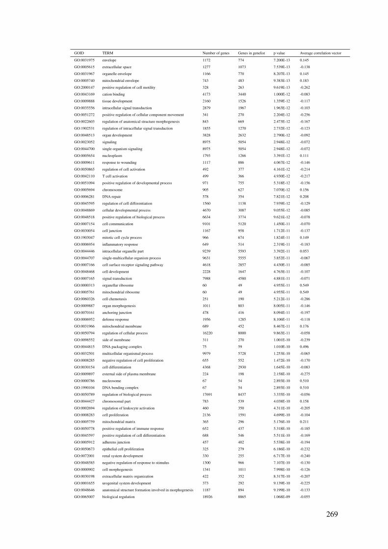
GOID TERM Number of genes Genes in genelist p value Average correlation vector
GO:0031975 envelope 1172 774 7.200E-13 0.145
GO:0005615 extracellular space 1277 1073 7.539E-13 -0.138
GO:0031967 organelle envelope 1166 770 8.207E-13 0.145
GO:0005740 mitochondrial envelope 743 483 9.383E-13 0.183
GO:2000147 positive regulation of cell motility 328 263 9.619E-13 -0.262
GO:0043169 cation binding 4173 3440 1.000E-12 -0.083
GO:0009888 tissue development 2160 1526 1.359E-12 -0.117
GO:0035556 intracellular signal transduction 2879 1967 1.963E-12 -0.103
GO:0051272 positive regulation of cellular component movement 341 270 2.204E-12 -0.256
GO:0022603 regulation of anatomical structure morphogenesis 843 669 2.473E-12 -0.167
GO:1902531 regulation of intracellular signal transduction 1855 1270 2.732E-12 -0.123
GO:0048513 organ development 3828 2632 2.790E-12 -0.092
GO:0023052 signaling 8975 5054 2.948E-12 -0.072
GO:0044700 single organism signaling 8975 5054 2.948E-12 -0.072
GO:0005654 nucleoplasm 1793 1266 3.391E-12 0.111
GO:0009611 response to wounding 1117 886 4.067E-12 -0.146
GO:0050865 regulation of cell activation 492 377 4.161E-12 -0.214
GO:0042110 T cell activation 499 366 4.930E-12 -0.217
GO:0051094 positive regulation of developmental process 971 755 5.318E-12 -0.156
GO:0005694 chromosome 905 627 7.070E-12 0.156
GO:0006281 DNA repair 578 354 7.821E-12 0.208
GO:0045595 regulation of cell differentiation 1560 1138 7.939E-12 -0.129
GO:0048869 cellular developmental process 4670 3087 9.055E-12 -0.085
GO:0048518 positive regulation of biological process 6634 3774 9.621E-12 -0.078
GO:0007154 cell communication 9101 5120 1.450E-11 -0.070
GO:0030054 cell junction 1167 958 1.712E-11 -0.137
GO:1903047 mitotic cell cycle process 966 674 1.824E-11 0.149
GO:0006954 inflammatory response 649 514 2.319E-11 -0.183
GO:0044446 intracellular organelle part 9239 5593 3.392E-11 0.053
GO:0044707 single-multicellular organism process 9631 5555 3.852E-11 -0.067
GO:0007166 cell surface receptor signaling pathway 4618 2857 4.430E-11 -0.085
GO:0048468 cell development 2228 1647 4.763E-11 -0.107
GO:0007165 signal transduction 7988 4580 4.881E-11 -0.071
GO:0000313 organellar ribosome 60 49 4.955E-11 0.549
GO:0005761 mitochondrial ribosome 60 49 4.955E-11 0.549
GO:0060326 cell chemotaxis 251 190 5.212E-11 -0.286
GO:0009887 organ morphogenesis 1011 803 8.005E-11 -0.146
GO:0070161 anchoring junction 478 416 8.094E-11 -0.197
GO:0006952 defense response 1956 1285 8.106E-11 -0.118
GO:0031966 mitochondrial membrane 689 452 8.467E-11 0.176
GO:0050794 regulation of cellular process 16220 8000 9.863E-11 -0.058
GO:0098552 side of membrane 311 270 1.001E-10 -0.239
GO:0044815 DNA packaging complex 75 59 1.010E-10 0.496
GO:0032501 multicellular organismal process 9979 5728 1.253E-10 -0.065
GO:0008285 negative regulation of cell proliferation 655 552 1.472E-10 -0.170
GO:0030154 cell differentiation 4368 2930 1.645E-10 -0.083
GO:0009897 external side of plasma membrane 224 198 2.158E-10 -0.275
GO:0000786 nucleosome 67 54 2.893E-10 0.510
GO:1990104 DNA bending complex 67 54 2.893E-10 0.510
GO:0050789 regulation of biological process 17691 8437 3.335E-10 -0.056
GO:0044427 chromosomal part 783 539 4.038E-10 0.158
GO:0002694 regulation of leukocyte activation 460 350 4.311E-10 -0.205
GO:0008283 cell proliferation 2136 1591 4.699E-10 -0.104
GO:0005759 mitochondrial matrix 365 296 5.176E-10 0.211
GO:0050778 positive regulation of immune response 652 437 5.318E-10 -0.185
GO:0045597 positive regulation of cell differentiation 688 546 5.511E-10 -0.169
GO:0005912 adherens junction 457 402 5.538E-10 -0.194
GO:0050673 epithelial cell proliferation 325 279 6.186E-10 -0.232
GO:0072001 renal system development 330 255 6.717E-10 -0.240
GO:0048585 negative regulation of response to stimulus 1300 966 7.107E-10 -0.130
GO:0000902 cell morphogenesis 1341 1011 7.998E-10 -0.126
GO:0030198 extracellular matrix organization 422 352 8.317E-10 -0.207
GO:0001655 urogenital system development 373 292 9.139E-10 -0.225
GO:0048646 anatomical structure formation involved in morphogenesis 1187 894 9.199E-10 -0.133
GO:0065007 biological regulation 18926 8865 1.068E-09 -0.055
269
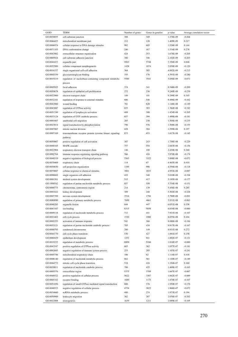
GOID TERM Number of genes Genes in genelist p value Average correlation vector
GO:0030055 cell-substrate junction 388 349 1.378E-09 -0.204
GO:0044455 mitochondrial membrane part 212 128 1.409E-09 0.317
GO:0006974 cellular response to DNA damage stimulus 982 605 1.526E-09 0.144
GO:0071103 DNA conformation change 246 167 1.534E-09 0.278
GO:0043062 extracellular structure organization 424 353 1.678E-09 -0.205
GO:0005924 cell-substrate adherens junction 380 346 2.102E-09 -0.203
GO:0044422 organelle part 9563 5748 2.356E-09 0.048
GO:0032989 cellular component morphogenesis 1428 1074 2.830E-09 -0.120
GO:0016337 single organismal cell-cell adhesion 364 305 4.002E-09 -0.215
GO:0005539 glycosaminoglycan binding 193 176 4.391E-09 -0.280
GO:0019219 regulation of nucleobase-containing compound metabolic
process
5589 3541 5.056E-09 -0.072
GO:0005925 focal adhesion 374 341 8.548E-09 -0.200
GO:0050678 regulation of epithelial cell proliferation 272 236 9.240E-09 -0.239
GO:0022900 electron transport chain 149 101 9.299E-09 0.345
GO:0032101 regulation of response to external stimulus 686 546 9.496E-09 -0.162
GO:0042060 wound healing 781 628 1.148E-08 -0.149
GO:0043087 regulation of GTPase activity 655 393 1.384E-08 -0.182
GO:0051249 regulation of lymphocyte activation 409 308 1.424E-08 -0.205
GO:0033124 regulation of GTP catabolic process 657 394 1.490E-08 -0.181
GO:0001667 ameboidal cell migration 285 238 1.504E-08 -0.235
GO:0023014 signal transduction by phosphorylation 790 576 1.509E-08 -0.155
GO:0007067 mitotic nuclear division 428 304 1.599E-08 0.197
GO:0007169 transmembrane receptor protein tyrosine kinase signaling
pathway
873 653 1.617E-08 -0.145
GO:0050867 positive regulation of cell activation 307 243 1.758E-08 -0.229
GO:0000165 MAPK cascade 757 554 2.043E-08 -0.156
GO:0022904 respiratory electron transport chain 146 100 2.430E-08 0.340
GO:0002764 immune response-regulating signaling pathway 566 416 3.870E-08 -0.174
GO:0048519 negative regulation of biological process 5363 3322 3.898E-08 -0.072
GO:0070469 respiratory chain 114 67 4.465E-08 0.410
GO:0030030 cell projection organization 1349 996 4.556E-08 -0.118
GO:0070887 cellular response to chemical stimulus 3061 2033 4.953E-08 -0.087
GO:0098602 single organism cell adhesion 422 340 5.010E-08 -0.194
GO:0001501 skeletal system development 515 417 5.195E-08 -0.177
GO:1900542 regulation of purine nucleotide metabolic process 857 558 5.334E-08 -0.151
GO:0000775 chromosome, centromeric region 214 139 5.456E-08 0.285
GO:0001822 kidney development 309 240 5.502E-08 -0.228
GO:0007399 nervous system development 2516 1794 5.790E-08 -0.091
GO:0080090 regulation of primary metabolic process 7699 4661 5.931E-08 -0.063
GO:0048285 organelle fission 644 447 6.051E-08 0.158
GO:0043167 ion binding 6315 5058 6.834E-08 -0.060
GO:0009118 regulation of nucleoside metabolic process 712 441 7.921E-08 -0.167
GO:0022402 cell cycle process 1520 1000 8.055E-08 0.104
GO:0002253 activation of immune response 541 366 8.088E-08 -0.184
GO:0033121 regulation of purine nucleotide catabolic process 705 434 9.917E-08 -0.167
GO:0000793 condensed chromosome 200 149 9.931E-08 0.272
GO:0044770 cell cycle phase transition 530 427 1.001E-07 0.158
GO:0060429 epithelium development 1252 941 1.002E-07 -0.121
GO:0019222 regulation of metabolic process 8809 5166 1.016E-07 -0.060
GO:0043547 positive regulation of GTPase activity 605 362 1.057E-07 -0.181
GO:0002683 negative regulation of immune system process 253 205 1.107E-07 -0.241
GO:0005746 mitochondrial respiratory chain 106 62 1.114E-07 0.418
GO:0006140 regulation of nucleotide metabolic process 862 561 1.120E-07 -0.149
GO:0044772 mitotic cell cycle phase transition 518 416 1.194E-07 0.160
GO:0030811 regulation of nucleotide catabolic process 706 435 1.469E-07 -0.165
GO:0005576 extracellular region 5375 3709 1.667E-07 -0.067
GO:0048522 positive regulation of cellular process 5622 3387 1.842E-07 -0.069
GO:0005102 receptor binding 1689 1175 1.870E-07 -0.107
GO:0051056 regulation of small GTPase mediated signal transduction 606 376 1.950E-07 -0.176
GO:0048523 negative regulation of cellular process 4754 3022 1.968E-07 -0.072
GO:0034660 ncRNA metabolic process 400 274 1.973E-07 0.194
GO:0050900 leukocyte migration 362 287 2.076E-07 -0.202
GO:0022008 neurogenesis 1639 1211 2.089E-07 -0.105
270

Appendix C
Nanostring gene set
Table C.1: All the genes measured in the nanostring gene set described in Section 4.4.2.1 withdescription of groups. Also included is the PGC induction score for each gene fromMitoCarta
Genes TF
net-
work
MitoCarta PGC
in-
duced
P53
in-
duced
mtDNA Control ETC Cytosolic
Ribo-
some.
Mito
ribosome
LFC
NRIP1 Yes No No No No 0 No No
PPRC1 Yes No No No No 0 No No
PPARGC1A Yes No No No No 0 No No
PPARGC1B Yes No No No No 0 No No
PPARG Yes No No No No 0 No No
PPARD Yes No No No No 0 No No
PPARA Yes No No No No 0 No No
ESRRA Yes No No No No 0 No No
ESRRB Yes No No No No 0 No No
ESRRG Yes No No No No 0 No No
GABPA Yes No No No No 0 No No
NRF1 Yes No No No No 0 No No
YY1 Yes No No No No 0 No No
CREB Yes No No No No 0 No No
MYC Yes No No No No 0 No No
PRMT1 Yes No No No No 0 No No
TFAM Yes Yes 4 No No No 0 No No
TFB1M Yes Yes No No No 0 No No
TFB2M Yes Yes No No No 0 No No
MEF2A Yes No No No No 0 No No
MYOD1 Yes No No No No 0 No No
FOXO1 Yes No No No No 0 No No
CDK7 Yes No No No No 0 No No
SIRT1 Yes No No No No 0 Yes No
FBXW7 Yes No No No No 0 No No
KAT2A Yes No No No No 0 No No
MYBBP1A Yes No No No No 0 No No
ELK1 Yes No No No No 0 No No
E2F1 Yes No No No No 0 No No
TP53 Yes No No No No 0 No No
SRF Yes No No No No 0 No No
PPARGC1A B5 -NT Yes No No No No 0 No No
ALDH5A1 No Yes 0 No No No 0 No No Mito upper fork pos LFC
BDH1 No Yes 16 No No No 0 No No Mito upper fork pos LFC
VAMP8 No Yes 2 No No No 0 No No Mito upper fork pos LFC
HSD17B8 No Yes 2 No No No 0 No No Mito upper fork pos LFC
GPT2 No Yes 0 No No No 0 No No Mito upper fork pos LFC
PXMP2 No Yes 2 No No No 0 No No Mito upper fork pos LFC
NTHL1 No Yes 0 No No No 0 No No Mito upper fork pos LFC
271

Genes TF
net-
work
MitoCarta PGC
in-
duced
P53
in-
duced
mtDNA Control ETC Cytosolic
Ribo-
some.
Mito
ribosome
LFC
OGDHL No Yes No No No 0 No No Mito upper fork pos LFC
AKAP1 No Yes 3 No No No 0 No No Mito upper fork pos LFC
SLC25A10 No Yes 0 No No No 0 No No Mito upper fork pos LFC
MRPL12 No Yes 4 No No No 0 No Yes Mito upper fork pos LFC
DHTKD1 No Yes 0 No No No 0 No No Mito upper fork pos LFC
TIMM8A No Yes 4 No No No 0 No No Mito upper fork pos LFC
SFXN4 No Yes 0 No No No 0 No No Mito upper fork pos LFC
L2HGDH No Yes 4 No No No 0 No No Mito upper fork pos LFC
TSHZ3 No Yes 0 No No No 0 No No Mito upper fork neg LFC
SLC25A24 No Yes No No No 0 No No Mito upper fork neg LFC
FTH1 No Yes 1 No No No 0 No No Mito upper fork neg LFC
ME1 No Yes No No No 0 No No Mito upper fork neg LFC
DDAH1 No Yes 0 No No No 0 No No Mito upper fork neg LFC
CYB5R2 No Yes No No No 0 No No Mito upper fork neg LFC
RAB11FIP5 No Yes 1 No No No 0 No No Mito upper fork neg LFC
HSPB7 No Yes 2 No No No 0 No No Mito upper fork neg LFC
TSPO No Yes 1 No No No 0 No No Mito upper fork neg LFC
ATP10D No Yes 2 No No No 0 No No Mito upper fork neg LFC
CLIC4 No Yes 1 No No No 0 No No Mito upper fork neg LFC
HK1 No Yes 0 No No No 0 No No Mito upper fork neg LFC
GALC No Yes 2 No No No 0 No No Mito upper fork neg LFC
CKMT2 No Yes 15 No No No 0 No No Mito upper fork neg LFC
ACOT9 No Yes 0 No No No 0 No No Mito upper fork neg LFC
ICT1 No Yes 2 No No No 0 No Yes
MRPS25 No Yes 7 No No No 0 No Yes
MRPL11 No Yes 2 No No No 0 No Yes
MRPS12 No Yes 2 No No No 0 No Yes
MRPL13 No Yes 2 No No No 0 No Yes
MRPS26 No Yes 2 No No No 0 No Yes
MRPS33 No Yes 1 No No No 0 No Yes
MRPS17 No Yes 2 No No No 0 No Yes
MRPS18B No Yes 2 No No No 0 No Yes
MRPS36 No Yes 2 No No No 0 No Yes
MRPS15 No Yes 1 No No No 0 No Yes
MRPL48 No Yes 2 No No No 0 No Yes
MRPL27 No Yes 1 No No No 0 No Yes
MRPL37 No Yes 2 No No No 0 No Yes
H2AFZ No No No No No 0 No No Non mito upper fork pos LFC
SNRPC No No No No No 0 No No Non mito upper fork pos LFC
PPIL1 No No No No No 0 No No Non mito upper fork pos LFC
SNRPF No No No No No 0 No No Non mito upper fork pos LFC
NUDT5 No No No No No 0 No No Non mito upper fork pos LFC
PAICS No No No No No 0 No No Non mito upper fork pos LFC
POLR3K No No No No No 0 No No Non mito upper fork pos LFC
RPA3 No No No No No 0 No No Non mito upper fork pos LFC
PSMA5 No No No No No 0 No No Non mito upper fork pos LFC
POLR2D No No No No No 0 No No Non mito upper fork pos LFC
THOC4 No No No No No 0 No No Non mito upper fork pos LFC
RAD51C No No No No No 0 No No Non mito upper fork pos LFC
EBP No No No No No 0 No No Non mito upper fork pos LFC
NUP85 No No No No No 0 No No Non mito upper fork pos LFC
DLC1 No No No No No 0 No No Non mito upper fork neg LFC
PHLDB1 No No No No No 0 No No Non mito upper fork neg LFC
PTRF No No No No No 0 No No Non mito upper fork neg LFC
AFAP1 No No No No No 0 No No Non mito upper fork neg LFC
AHR No No No No No 0 No No Non mito upper fork neg LFC
MFGE8 No No No No No 0 No No Non mito upper fork neg LFC
CHST3 No No No No No 0 No No Non mito upper fork neg LFC
VCL No No No No No 0 No No Non mito upper fork neg LFC
ZNF223 No No No No No 0 No No Non mito upper fork neg LFC
CCBE1 No No No No No 0 No No Non mito upper fork neg LFC
ARHGAP21 No No No No No 0 No No Non mito upper fork neg LFC
EHD2 No No No No No 0 No No Non mito upper fork neg LFC
272

Genes TF
net-
work
MitoCarta PGC
in-
duced
P53
in-
duced
mtDNA Control ETC Cytosolic
Ribo-
some.
Mito
ribosome
LFC
DSEL No No No No No 0 No No Non mito upper fork neg LFC
NAV2 No No No No No 0 No No Non mito upper fork neg LFC
COL16A1 No No No No No 0 No No Non mito upper fork neg LFC
RPL38 No No No No No 0 No Yes
EIF4A3 No No No No No 0 Yes No
EXOSC5 No No No No No 0 Yes No
RPL30 No No No No No 0 Yes No
RPL8 No No No No No 0 Yes No
WDR12 No No No No No 0 Yes No
RPS21 No No No No No 0 Yes No
NHP2L1 No No No No No 0 Yes No
APEX1 No No No No No 0 Yes No
SRP68 No No No No No 0 Yes No
RRP1B No No No No No 0 Yes No
EXOSC4 No No No No No 0 Yes No
NOLC1 No No No No No 0 Yes No
RRS1 No No No No No 0 Yes No
UTP18 No No No No No 0 Yes No
MRPL15 No Yes 3 No No No 0 No Yes
MRPL34 No Yes 3 No No No 0 No Yes
ATP5C1 No Yes 3 No No No V No No
ATP5O No Yes 3 No No No V No No
ATP5A1 No Yes 3 No No No V No No
COX5B No Yes 3 No No No IV No No
COX7B No Yes 3 No No No IV No No
COX11 No Yes 6 No No No IV No No
NDUFB5 No Yes 3 No No No I No No
NDUFA6 No Yes 3 No No No I No No
NDUFB10 No Yes 4 No No No I No No
NDUFS3 No Yes 3 No No No I No No
ACTA2 No No Yes No No 0 No No
APAF1 No No Yes No No 0 No No
ARID3A No No Yes No No 0 No No
BAX No Yes 0 Yes No No 0 No No
BID No Yes 2 Yes No No 0 No No
CASP1 No No Yes No No 0 No No
CAV1 No No Yes No No 0 No No
CTSD No No Yes No No 0 No No
DNMT1 No No Yes No No 0 No No
EEF1A1 No No Yes No No 0 No No
FAS No No Yes No No 0 No No
HIC1 No No Yes No No 0 No No
IRF5 No No Yes No No 0 No No
KRT8 No No Yes No No 0 No No
LGALS3 No No Yes No No 0 No No
LRDD No No Yes No No 0 No No
MMP2 No No Yes No No 0 No No
PMS2 No No Yes No No 0 No No
PTK2 No No Yes No No 0 No No
PYCARD No No Yes No No 0 No No
RFWD2 No No Yes No No 0 No No
SCD No No Yes No No 0 No No
TGFA No No Yes No No 0 No No
PUMA No No Yes No No 0 No No
PMAIP1 (NOXA) No No Yes No No 0 No No
SCD5 No No No No Yes 0 No No
CCDC85B No No No No Yes 0 No No
ARF1 No No No No Yes 0 No No
SUMO3 No No No No Yes 0 No No
MT-CO1 No No No Yes No IV No No
MT-CO2 No No No Yes No IV No No
MT-CYB No No No Yes No III No No
MT-ND1 No No No Yes No I No No
273

Genes TF
net-
work
MitoCarta PGC
in-
duced
P53
in-
duced
mtDNA Control ETC Cytosolic
Ribo-
some.
Mito
ribosome
LFC
MT-ND2 No No No Yes No I No No
MT-ND3 No No No Yes No I No No
MT-ND4 No No No Yes No I No No
MT-ND4L No No No Yes No I No No
MT-ND5 No No No Yes No I No No
MT-ND6 No No No Yes No I No No
274

Appendix D
Materials
Below is a table of the materials used in this thesis
Table D.1: Table of materials used in this thesis.
Material Source Other infor-
mation
Tissue culture
DMEM Gibco 31966-021
Fetal bovine serum Gibco 10500-064
Glutamax Gibco 35050-038
Normocin InvivoGen ant-nr-2
Trypan blue Gibco 15250-061
Trysin Gibco 25200-056 0.25%
Antibodies
GAPDH Santa Cruz sc-25778
b -tubulin Santa Cruz sc-9104
GRP75 Santa Cruz sc-1058 1:2000
Oxphos cocktail Novex 458199 1:1000
Western blots
Blotting pads Invitrogen LC2010
ECL GE Healthcare PRN2106
Ladder BioRad 161-0375
MES running buffer Novex NP0002 20X
NuPAGE 10% gels Novex NP0301BOX 1mmx10wells
275

Material Source Other infor-
mation
NuPAGE LDS Sample buffer Novex NP0007 4X
Ponceau S Sigma P7170
PVDF membranes Immobilin P IPVH00010
Transfer buffer Novex NP0006 20X
Tween Sigma P1379
Kits
RNeasy Mini Kit Qiagen 74106
Chemicals
Antimycin A Sigma A8674
Carbonyl cyanide-4-
(trifluoromethoxy) phenylhy-
drazone (FCCP)
Sigma C2920
DMEM powder Sigma D5030
Glucose Sigma G8270
Oligomycin Sigma 75371
Phoshate buffered saline
(PBS)
Gibco 14190-094
Sodium pyruvate Sigma P8574
Nanostring
nCounter Master Kit Nanostring technologies NAA-
AKIT-192
nCounter Gene Expression
(GX) CodeSet
Nanostring technologies GXA-
P1CS-096
GC-MC
scyllo-Inositol Sigma I8132
Nor-leucine Sigma N8513
Methoxyamine hydrochloride Sigma 226904
Pyridine Sigma 270970
BSTFA + TMCS Supleco 33155-U 99:1
276
Related Documents