A bijective proof of Macdonald’s reduced word formula · Discrete Mathematics and Theoretical Computer Science DMTCS vol. (subm.), by the authors, 1–1 A bijective proof of Macdonald’s

Discrete Mathematics and Theoretical Computer Science DMTCS vol. (subm.), by the authors, 1–1

A bijective proof of Macdonald’s reducedword formula

Sara C. Billey1† and Alexander E. Holroyd2‡ and Benjamin J. Young2§

1Department of Mathematics, University of Washington, Box 354350, Seattle, WA 98195, USA2Microsoft Research, 1 Microsoft Way, Redmond, WA 98052, USA 3Department of Mathematics, 1222 University ofOregon, Eugene, OR 97403

received 2015-11-16, revised 2016-3-29, accepted 2016-2-11.

We describe a bijective proof of Macdonald’s reduced word identity using pipe dreams and Little’s bumping al-gorithm. The proof extends to a principal specialization of the identity due to Fomin and Stanley. Our bijectivetools also allow us to address a problem posed by Fomin and Kirillov from 1997, using work of Wachs, Lenart andSerrano-Stump.

Nous donnons une preuve bijective de l’identite des mots reduits de Macdonald, en utilisant des “pipe dreams” etl’algorithme “bumping” de Little. La preuve est etendue a une specialisation principale de l’identite due a Fominet Stanley. La methode bijective nous permet aussi de traiter un probleme pose par Fomin et Kirillov en 1997, enutilisant les travaux de Wachs, Lenart et Serrano-Stump.

Keywords: reduced words, Schubert polynomials, RC graphs, pipe dreams, bijective proof, algorithmic bijection

1 IntroductionMacdonald gave a remarkable formula connecting a weighted sum of reduced words for permutationswith the number of terms in a Schubert polynomial Sπ(x1, . . . , xn). For a permutation π ∈ Sn, let `(π)be its inversion number and let R(π) denote the set of its reduced words. (See Section 2 for definitions.)

Theorem 1.1 (Macdonald [Mac91, (6.11)]) Given a permutation π ∈ Sn with `(π) = p, one has∑(a1,a2,...,ap)∈R(π)

a1 · a2 · · · ap = p! Sπ(1, . . . , 1). (1.1)

For example, the permutation [3, 2, 1] ∈ S3 has 2 reduced words, R([3, 2, 1]) = {(1, 2, 1), (2, 1, 2)}.The inversion number is `([3, 2, 1]) = 3, and the Schubert polynomial Sπ is the single term x21x2. Weobserve that Macdonald’s formula holds: 1 · 2 · 1 + 2 · 1 · 2 = 3! · 1.

†Email: [email protected]. Billey was partially supported by grant DMS-1101017 from the NSF.‡Email: [email protected].§Email: [email protected].

subm. to DMTCS c© by the authors Discrete Mathematics and Theoretical Computer Science (DMTCS), Nancy, France

2 Sara C. Billey and Alexander E. Holroyd and Benjamin J. Young

1234

1 4 3 21234

3 1 4 21234

3 1 2 41234

2 1 3 41234

1 2 3 4

_ _ 1 _ _ _1 _ 21 1 22 1 2

1

2

3

4

1

2

3

4

1

2

3

4

1

2

3

4

1

2

3

4

1

2

3

4

1

2

3

4

1

3

2

4

1

3

4

2

4

1

3

2

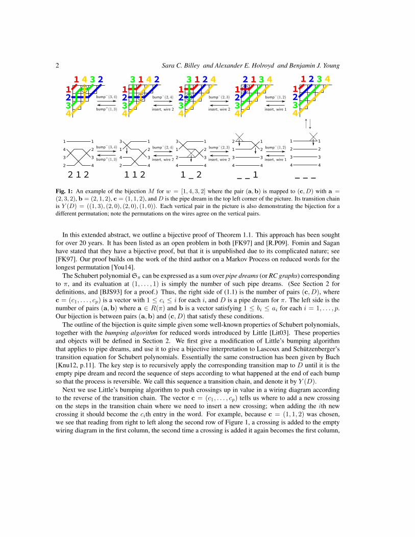
Fig. 1: An example of the bijection M for w = [1, 4, 3, 2] where the pair (a,b) is mapped to (c, D) with a =(2, 3, 2), b = (2, 1, 2), c = (1, 1, 2), and D is the pipe dream in the top left corner of the picture. Its transition chainis Y (D) = ((1, 3), (2, 0), (2, 0), (1, 0)). Each vertical pair in the picture is also demonstrating the bijection for adifferent permutation; note the permutations on the wires agree on the vertical pairs.

In this extended abstract, we outline a bijective proof of Theorem 1.1. This approach has been soughtfor over 20 years. It has been listed as an open problem in both [FK97] and [R.P09]. Fomin and Saganhave stated that they have a bijective proof, but that it is unpublished due to its complicated nature; see[FK97]. Our proof builds on the work of the third author on a Markov Process on reduced words for thelongest permutation [You14].

The Schubert polynomial Sπ can be expressed as a sum over pipe dreams (or RC graphs) correspondingto π, and its evaluation at (1, . . . , 1) is simply the number of such pipe dreams. (See Section 2 fordefinitions, and [BJS93] for a proof.) Thus, the right side of (1.1) is the number of pairs (c, D), wherec = (c1, . . . , cp) is a vector with 1 ≤ ci ≤ i for each i, and D is a pipe dream for π. The left side is thenumber of pairs (a,b) where a ∈ R(π) and b is a vector satisfying 1 ≤ bi ≤ ai for each i = 1, . . . , p.Our bijection is between pairs (a,b) and (c, D) that satisfy these conditions.

The outline of the bijection is quite simple given some well-known properties of Schubert polynomials,together with the bumping algorithm for reduced words introduced by Little [Lit03]. These propertiesand objects will be defined in Section 2. We first give a modification of Little’s bumping algorithmthat applies to pipe dreams, and use it to give a bijective interpretation to Lascoux and Schutzenberger’stransition equation for Schubert polynomials. Essentially the same construction has been given by Buch[Knu12, p.11]. The key step is to recursively apply the corresponding transition map to D until it is theempty pipe dream and record the sequence of steps according to what happened at the end of each bumpso that the process is reversible. We call this sequence a transition chain, and denote it by Y (D).

Next we use Little’s bumping algorithm to push crossings up in value in a wiring diagram accordingto the reverse of the transition chain. The vector c = (c1, . . . , cp) tells us where to add a new crossingon the steps in the transition chain where we need to insert a new crossing; when adding the ith newcrossing it should become the cith entry in the word. For example, because c = (1, 1, 2) was chosen,we see that reading from right to left along the second row of Figure 1, a crossing is added to the emptywiring diagram in the first column, the second time a crossing is added it again becomes the first column,

Macdonald’s reduced word formula 3

and the third time a crossing is added it becomes the second column. The row of the added crossing isdetermined by placing its feet on the wire specified by the corresponding step of the transition chain. Eachnew crossing is immediately pushed up in value, initiating a Little bump. The result is a reduced wiringdiagram for π corresponding to a reduced word a = (a1, a2, . . . , ap). If we bumping processes, we obtaina vector b = (b1, . . . , bp) of the same length such that ai ≥ bi for all i, as required. See Figure 1 for anillustration of the algorithm. Each step is reversible.

A computer implementation of this bijection will be made available at http://www.math.washington.edu/˜billey/papers/macdonald/.

1.1 Further results: q-analogOur bijective proof extends to a q-analog of (1.1) that was conjectured by Macdonald and subsequentlyproved by Fomin and Stanley. To state this formula, let q be a formal variable. Define the q-analog of apositive integer k to be [k] = [k]q := (1+ q+ q2+ · · ·+ qk−1). The q-analog of the factorial k! is definedto be [k]! = [k]q! := [k][k − 1] · · · [1]. (We use the blackboard bold symbol ! to distinguish it from theordinary factorial of k.) For a = (a1, a2, . . . , ap) ∈ R(π), define the co-major index

comaj(a) :=∑

1≤i≤p:ai<ai+1

i.

Theorem 1.2 (Fomin and Stanley [FS94, Thm. 2.4]) Given a permutation π ∈ Sn with `(π) = p, onehas ∑

a=(a1,a2,...,ap)∈R(π)

[a1] · [a2] · · · [ap] qcomaj(a) = [p] ! Sπ(1, q, q2, . . . , qn−1). (1.2)

Continuing with the example π = [3, 2, 1], we observe that the q-analog formula indeed holds: q[1] ·[2] · [1]+ q2[2] · [1] · [2] = q(1+ q)+ q2(1+ q)2 = q+2q2+2q3+ q4 = [3] ! ·q = [3] ! ·S[3,2,1](1, q, q

2).Our proof of Theorem 1.2 is omitted from this abstract due to space constraints. Our approach is to

define statistics on (a,b) pairs and on (c,D) pairs, and interpret the left and right sides of Theorem 1.2 asa statement about the corresponding generating functions. We then show that our map M preserves thesestatistics.

1.2 Further results: Fomin-Kirillov identityIn 1997, Fomin and Kirillov published an extension to Theorem 1.2 in the case where π is a dominantpermutation whose Rothe diagram is the partition λ (see Section 2 for definitions of these terms). To stateit we need the following definitions:

Let rppλ(x) be the set of weak reverse plane partitions whose entries are all in the range [0, x] forx ∈ N. This is the set of x-bounded fillings of λ with rows and columns weakly increasing to the rightand down. Given a weak reverse plane partition R, let |R| be the sum of its entries. Let

[rppλ(x)]q =∑

R∈rppλ(x)

q|R|.

Finally, for π = [π1, . . . , πn], let 1x × π = [1, 2, . . . , x, π1 + x, π2 + x, . . . , πn + x].

4 Sara C. Billey and Alexander E. Holroyd and Benjamin J. Young

Theorem 1.3 [FK97, Thm. 3.1] For any partition λ ` p, we have the following identity for all x ∈ N∑(a1,a2,...,ap)∈R(σλ)

qcomaj(a1,a2,...,ap)[x+ a1] · [x+ a2] · · · [x+ ap] (1.3)

= [p] ! S1x×σλ(1, q, q2, . . . , qx+p) (1.4)

= [p] ! qb(λ) [rppλ(x)]q (1.5)

where b(λ) =∑i(i− 1)λi.

Fomin-Kirillov proved this non-bijectively, using known results from Schubert calculus, and asked fora bijective proof. Using our results, together with results of Lenart [Len04], and Serrano and Stump[SS11, SS12], we are able to provide a bijective proof. We omit this proof from the abstract. See also[BJS93, Woo04] for connections to plane partitions.

2 Background2.1 PermutationsWe recall some basic notation and definitions relating to permutations which are standard in the theory ofSchubert polynomials. We refer the reader to [LS82, Mac91, Man01] for references.

For π ∈ Sn, an inversion of π is an ordered pair (i, j), with 1 ≤ i < j ≤ n, such that π(i) > π(j).The length `(π) is the number of inversions of π. We write tij for the transposition which swaps i and j,and we write si = ti,i+1 (1 ≤ i ≤ n− 1). The si are called simple transpositions; they generate Sn as aCoxeter group.

We will often write a permutation π in one-line notation, [π(1), π(2), . . . , π(n)]. If π(j) > π(j + 1),then we say that π has a descent at j.

An alternate notation for a permutation π is its Lehmer code, or simply code, which is n-tuple

(L(π)1, L(π)2, . . . , L(π)n)

where L(π)i denotes the number of inversions (i, j) with the first coordinate fixed. The permutation π issaid to be dominant if its code is a weakly decreasing sequence.

2.2 Reduced wordsLet π ∈ Sn be a permutation. A word for π is a k-tuple of numbers a = (a1, . . . , ak) (1 ≤ ai < n) suchthat

sa1sa2 . . . sak = π.

Throughout this paper we will identify Sn with its image under the standard embedding ι : Sn ↪→ Sn+1;observe that this map sends Coxeter generators to Coxeter generators, so a word for π is also a word forι(π). If k = `(π), then we say that a is reduced. The reduced words are precisely the minimum-lengthways of representing π in terms of the simple transpositions. For instance, the permutation 321 ∈ S3 hastwo reduced words: 121 and 212.

WriteR(π) for the set of all reduced words of the permutation π. The setR(π) has received much study,largely due to interest in Bott-Samelson varieties and Schubert calculus. Its size has an interpretation interms of counting standard tableaux and the Stanley symmetric functions [LS82, Lit03, Sta84, EG87].

Macdonald’s reduced word formula 5

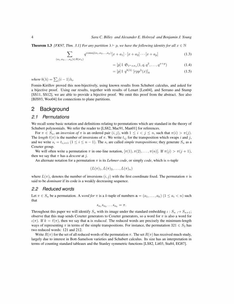
Fig. 2: The wiring diagram for the reduced word (4, 3, 5, 6, 4, 3, 5) ∈ R([1, 2, 6, 5, 7, 3, 4]) showing the intermediatepermutations on the left and a simplified version of the same wiring diagram on the right. The crossings in positions2 and 6 are both in row 3.

7

6

5

4

3

2

1

7

6

4

5

3

2

1

7

6

4

3

5

2

1

7

4

6

3

5

2

1

4

7

6

3

5

2

1

4

7

3

6

5

2

1

4

7

3

5

6

2

1

4

3

7

5

6

2

1 1

2

3

4

5

6

7

7

1

2

3

4

5

6

Define the wiring diagram for a word a as follows. First, for 0 ≤ t ≤ k, define πt ∈ Sn by

πt = sa1sa1 · · · sat .

In particular, when t = 0 the product on the right is empty, so that π0 is the identity permutation. Also,πk = π. The ith wire of a is defined to be the piecewise linear path joining the points (πt(i), t) for0 ≤ t ≤ k. We will consistently use “matrix coordinates” to describe wiring diagrams, so that (i, j) refersto row i (numbered from the top of the diagram) and column j (numbered from the left). The wiringdiagram is the union of these n wires. See Figure 2 for an example.

For all t ≥ 1, observe that between columns t−1 and t in the wiring diagram, precisely two wires i andj intersect. This configuration is called a crossing. One can identify a crossing by its position t. When theword a is reduced, the minimality of the length of a ensures that any two wires cross at most once. In thiscase, we can also identify a crossing by the unordered pair {i, j} of wires which are involved. In a wiringdiagram, we call at the row of the crossing at position t.

2.3 Little’s bumping algorithm

Little’s algorithm [Lit03] is a map on reduced words. It was introduced to study the decomposition ofStanley symmetric functions into Schur functions in a bijective way. Later, Little’s algorithm was foundto be related to the RSK [Lit05] and Edelman-Greene [HY14] algorithms; it has been extended to signedpermutations [BHRY14] and affine permutations [LS05]. We describe here a variant of the algorithm,which is the key building block for our bijective proofs. Our exposition follows that of [You14].

Definition 2.1 Let a = (a1, . . . , ak) be a word. Define the push up, push down and deletion of a at

6 Sara C. Billey and Alexander E. Holroyd and Benjamin J. Young

position t, respectively, to be

P−t a = (a1, . . . , at−1, at − 1, at+1, . . . , ak),

P+t a = (a1, . . . , at−1, at + 1, at+1, . . . , ak),

Dta = (a1, . . . , at−1, at+1, . . . , ak).

In [You14], the notation P↑ was used to represent P−, and P↓ was used to represent P+.

Definition 2.2 Let a be a word. If Dta is reduced, then we say that a is nearly reduced at t.

The term “nearly reduced” was coined by Lam et al [LLM+14, Chapter 3], who uses “t-marked nearlyreduced”. Words that are nearly reduced at t may or may not also be reduced; however, every reducedword a is nearly reduced at some index t. For instance, any reduced word a of length k is nearly reducedat 1 and also at k.

In order to define our variant of Little’s bumping map, we need the following lemma, which to ourknowledge first appeared in [Lit03, Lemma 4], and was later generalized to arbitrary Coxeter systemsin [LS05, Lemma 21].

Lemma 2.3 If a is not reduced, but is nearly reduced at t, then a is nearly reduced at exactly one otherposition t′ 6= t.

Definition 2.4 In the situation of Lemma 2.3, we say that t′ forms a defect with t in a, and writeDefectt(a) = t′.

Note that in Definition 2.4, in the wiring diagram of a, the two wires crossing in position t cross inexactly one other position t′.

Definition 2.5 A word b is a bounded word for another word a if the words have the same length and1 ≤ bi ≤ ai for all i. A bounded pair (for a permutation π) is an ordered pair (a,b) such that a is areduced word (for π) and b is a bounded word for a. Let BoundedPairs(π) be the set of all boundedpairs for π.

Algorithm 2.6 (Bounded Bumping Algorithm) The following is a modification of Little’s generalizedbumping algorithm, defined in [Lit03]. See Figure 3 for an example.Input: (a′,b′, t0, d), where a′ is a word that is nearly reduced at t0, b′ is a bounded word for a′, andd ∈ {−,+} is a direction.Output: (a,b, i, t), where a is a reduced word, b is a bounded word for a, i is a wire number, and t is aposition.

1. Initialize a← a′,b← b′, t← t0.

2. a←Pdt a, b←Pd

t b.

3. If bt = 0, let i be the larger-numbered of the two wires swapped by the crossing at position t of a.Return (Dta,Dtb, i, t) and stop.

4. If a is reduced, return (a,b, i, 0) and stop.

5. t← Defectt(a); Go to step 2.

Macdonald’s reduced word formula 7

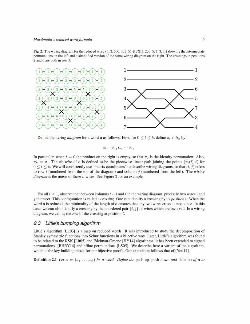
Fig. 3: An example of the Little bump algorithm with inputs (a,b, 4,−), with a = (4, 3, 5, 6, 4, 3, 5) and b = a.The arrows indicate which crossing will move up in the next step.

Observe that a need not be a reduced word in order for Algorithm 2.6 to be well-defined. Rather, a needonly be nearly reduced at t0. Note also that the algorithm only halts in step 3 when d = −.

There are two significant differences between Little’s map θr in [Lit03] and the map defined by Al-gorithm 2.6, other than the indexing. One difference is that θr shifts the entire word down (by applying∏t P

+t , in our terminology) if a crossing is pushed onto the zero line, whereas Algorithm 2.6 does not;

our step 3 prevents this situation from occurring. The second difference is that Little’s map acts only onthe word and not its bounded word; Little’s map does not have an equivalent of step 3.

Since the algorithm for Little’s θr terminates [Lit03], so does Algorithm 2.6. Similarly, if Algorithm 2.6is applied to (a′,b′) and terminates during step 4 returning (a,b, i, 0), then comaj(a) = comaj(a′); thisis essentially because Little’s map θr also preserves the comajor index (and indeed the descent set). If itterminates during step 3, the algorithm has a complicated effect on comaj a, whose description we omitfrom this abstract; it is needed for our proof of Theorem 1.2.

2.4 Pipe Dreams and Schubert PolynomialsSchubert polynomials Sπ for π ∈ Sn are a generalization of Schur polynomials that were invented byLascoux and Schutzenberger in the early 1980s [LS82]. They have been widely used over the past 30years in research. An excellent summary of the early work on these polynomials appears in Macdonald’s“Notes on Schubert polynomials” [Mac91]; see also the book by Manivel for a more recent treatment[Man01].

A pipe dream D is a finite subset of Z+ × Z+. We will usually draw a pipe dream as a modifiedwiring diagram as follows. Place a + at every point (i, j) ∈ D; place a pair of elbows at every point(i, j) ∈ Z+ × Z+ \D. This creates wires connecting points on the left side of the diagram to points on

8 Sara C. Billey and Alexander E. Holroyd and Benjamin J. Young

52134

5

2

5

6

4

1

3

1 2 3 4 5 6

Fig. 4: A reduced pipe dream for w = [3, 1, 4, 6, 5, 2]. The corresponding reduced word is a = (5, 2, 1, 3, 4, 5) andxD = x31x2x3x5.

the top. If the wires are numbered 1, 2, 3, . . . across the top of the diagram, then the corresponding wiresreading down the left side of the diagram form a finitely supported permutation π of the positive integerscalled the permutation of D; again, we identify Sn with its image under the inclusion Sn ↪→ SN, and thusthe finiteness of D means that π ∈ Sn for some n. We only need to draw a finite number of wires ina triangular array to represent a pipe dream since for all large enough wires there are no crossings. SeeFigure 4 for an example.

Following the terminology for reduced words, we say that D is reduced if π is the permutation of D,and `(π) = |D|. We write RP(π) for the set of all reduced pipe dreams for π. We say that the weight ofa pipe dream D is

xD =∏

(i,j)∈D

xi

where x1, x2, . . . are formal variables.

Definition 2.7 The Schubert polynomial of π ∈ Sn is defined to be

Sπ =∑

D∈RP(π)

xD.

For example, the top line of Figure 1 shows pipe dreams for 5 different permutations. The pipe dreamin the middle of the figure for [3, 1, 2, 4] is unique so S[3,1,2,4] = x1x2. The pipe dream on the left for[1, 4, 3, 2] is not the only one. There are 5 pipe dreams for w = [1, 4, 3, 2] in total and

S[1,4,3,2] = x21x2 + x21x3 + x1x2x3 + x22x3 + x1x22.

There are many other equivalent definitions of Schubert polynomials [LS82, BJS93, FS94, BB93].Note that pipe dreams are also called pseudo-line arrangements and RC-graphs in the literature. See[KM05, Kog00] for other geometric and algebraic interpretations of individual pipe dreams.

We call the elements of D ∈ RP(π) crossings or occupied positions, and the elements of (i, j) ∈Z+ × Z+ \ D unoccupied positions. Each crossing involves two wires, which are said to enter thecrossing horizontally and vertically.

As explained in [BB93], a reduced pipe dream D is precisely a reduced word together with some extrainformation about where to place the crossings. More precisely, if D is a reduced pipe dream, and we

Macdonald’s reduced word formula 9

replace each crossing (i, j) ∈ D with the value (j + i − 1) and then read the values along the rows ofD from right to left, and then read the rows top to bottom (see Figure 4, right picture), we get a reducedword for the permutation of D.

This map from pipe dreams to reduced words is not bijective; to obtain a bijection, we need to introducethe notion of compatible sequence from [BB93]. The compatible sequence is read from D by reading therow numbers of the crossings in the same order (reading the values along the rows of D right to left, andthen reading the rows top to bottom). Note the compatible sequence contains the same information as themonomial xD. The compatible sequences for the reduced word (a1, a2, . . . , ap) may be characterized asthe set of sequences (i1, i2, . . . , ip) which have the following three properties:

1. i1 ≤ i2 ≤ . . . ≤ ip,

2. aj < aj+1 implies ij < ij+1,

3. ij ≤ aj for all j.

For example, Figure 4 shows the pipe dream corresponding with reduced word (5, 2, 1, 3, 4, 5) andcompatible sequence (1, 1, 1, 2, 3, 5).

Finally, the bounded word associated to D is read from D by reading the column numbers of thecrossings, again in the same order. Observe that D can be reconstructed from its associated reduced wordand bounded word.

3 Transition equationTo describe the bijection M from cD-pairs to bounded pairs, we will first consider a sequence of pipedreams starting with D and moving toward the empty pipe dream. This is done using Algorithm 2.6,following steps from the transition equation due to Lascoux-Schutzenberger.

Theorem 3.1 (Lascoux and Schutzenberger, Transition Equation) [Mac91, 4.16] For all permutationsπ with `(π) > 0, the Schubert polynomial Sπ is determined by the recurrence

Sπ = xrSν +∑i<r

l(π)=l(νtir)

Sνtir (3.1)

where r is the last descent of π, s is the largest index such that πs < πr, ν = πtrs. The base case of therecurrence is Sid = 1.

Proof: (sketch) Algorithm 2.6 can be used to prove this theorem bijectively. Indeed, in this case, ouralgorithm coincides with an algorithm of Buch, described first in [Knu12, p.11].

Suppose that D′ is a pipe dream associated to π. Let (a′,b′) be the reduced word and bounded wordassociated to the pipe dream D′. Let π be the permutation associated to D′, and let r, s be as in Theo-rem 3.1. By construction, `(ν) = `(pi)−1 since the inversions of ν are exactly the same as the inversionsof π except for the pair (r, s). Therefore, if t′ is the position of the r, s-wire crossing in the wiring dia-gram for a, then a is nearly reduced in position t′. This is a key observation used in prior work as well[Lit03, LS82, Gar02]. Apply Algorithm 2.6 with arguments (a′,b′, t′,−), with output (a,b, i, t). Sinceb is encoding the column number, Algorithm 2.6 returns a pair (a,b) which is associated to a new pipe

10 Sara C. Billey and Alexander E. Holroyd and Benjamin J. Young

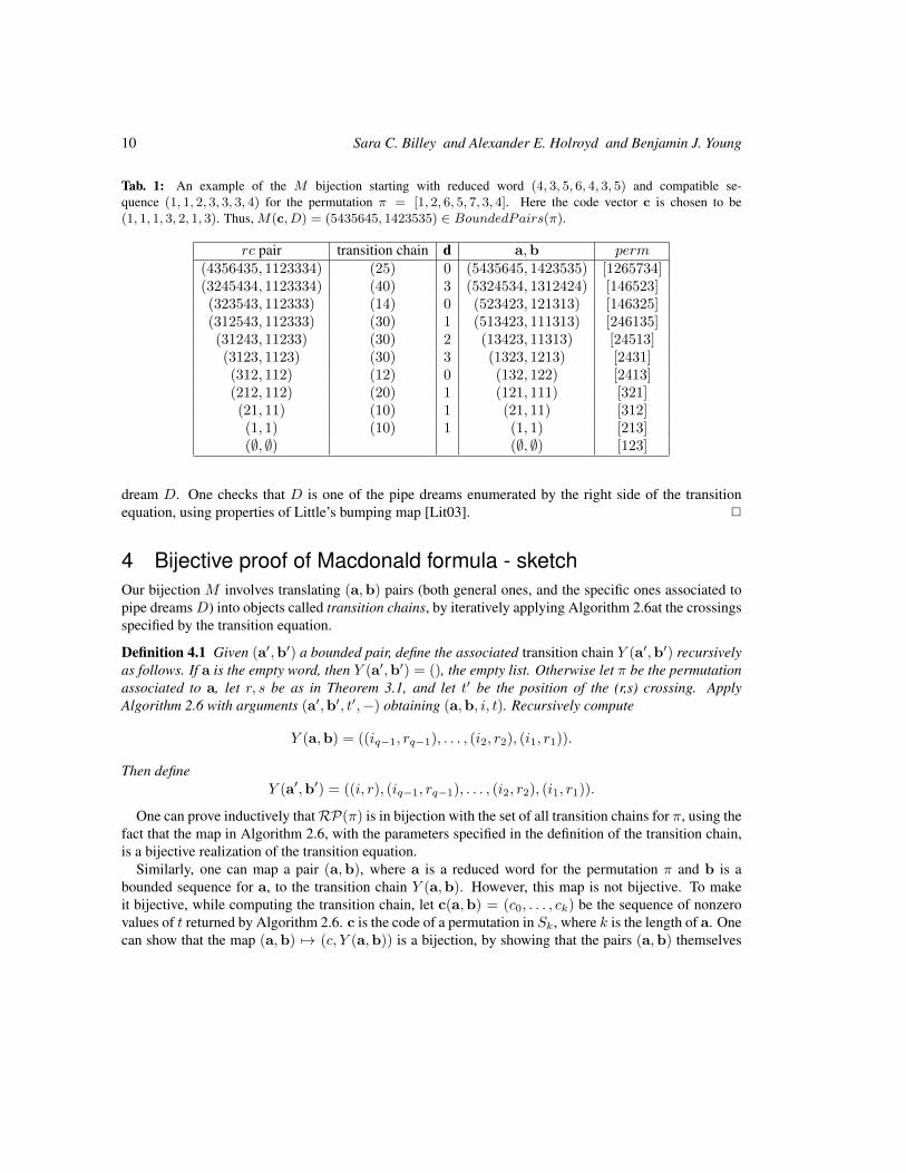
Tab. 1: An example of the M bijection starting with reduced word (4, 3, 5, 6, 4, 3, 5) and compatible se-quence (1, 1, 2, 3, 3, 3, 4) for the permutation π = [1, 2, 6, 5, 7, 3, 4]. Here the code vector c is chosen to be(1, 1, 1, 3, 2, 1, 3). Thus, M(c, D) = (5435645, 1423535) ∈ BoundedPairs(π).

rc pair transition chain d a,b perm(4356435, 1123334) (25) 0 (5435645, 1423535) [1265734](3245434, 1123334) (40) 3 (5324534, 1312424) [146523](323543, 112333) (14) 0 (523423, 121313) [146325](312543, 112333) (30) 1 (513423, 111313) [246135](31243, 11233) (30) 2 (13423, 11313) [24513](3123, 1123) (30) 3 (1323, 1213) [2431](312, 112) (12) 0 (132, 122) [2413](212, 112) (20) 1 (121, 111) [321](21, 11) (10) 1 (21, 11) [312](1, 1) (10) 1 (1, 1) [213](∅, ∅) (∅, ∅) [123]

dream D. One checks that D is one of the pipe dreams enumerated by the right side of the transitionequation, using properties of Little’s bumping map [Lit03]. 2

4 Bijective proof of Macdonald formula - sketchOur bijection M involves translating (a,b) pairs (both general ones, and the specific ones associated topipe dreamsD) into objects called transition chains, by iteratively applying Algorithm 2.6at the crossingsspecified by the transition equation.

Definition 4.1 Given (a′,b′) a bounded pair, define the associated transition chain Y (a′,b′) recursivelyas follows. If a is the empty word, then Y (a′,b′) = (), the empty list. Otherwise let π be the permutationassociated to a, let r, s be as in Theorem 3.1, and let t′ be the position of the (r,s) crossing. ApplyAlgorithm 2.6 with arguments (a′,b′, t′,−) obtaining (a,b, i, t). Recursively compute

Y (a,b) = ((iq−1, rq−1), . . . , (i2, r2), (i1, r1)).

Then defineY (a′,b′) = ((i, r), (iq−1, rq−1), . . . , (i2, r2), (i1, r1)).

One can prove inductively thatRP(π) is in bijection with the set of all transition chains for π, using thefact that the map in Algorithm 2.6, with the parameters specified in the definition of the transition chain,is a bijective realization of the transition equation.

Similarly, one can map a pair (a,b), where a is a reduced word for the permutation π and b is abounded sequence for a, to the transition chain Y (a,b). However, this map is not bijective. To makeit bijective, while computing the transition chain, let c(a,b) = (c0, . . . , ck) be the sequence of nonzerovalues of t returned by Algorithm 2.6. c is the code of a permutation in Sk, where k is the length of a. Onecan show that the map (a,b) 7→ (c, Y (a,b)) is a bijection, by showing that the pairs (a,b) themselves

Macdonald’s reduced word formula 11

satisfy a variant of the transition equation for bounded pairs. Unfortunately we need to omit the details ofthis argument.

Thus, the desired bijection which proves Macdonald’s reduced word identity is the composition of thefirst transition chain bijection with the inverse of the second.

Definition 4.2 Given (c,D) a CD pair, compute (a′,b′) associated to D, and then compute Y (a′,b′).Then, compute a new bounded pair (a,b) from Y (a′,b′), inserting the crossings at positions indicatedby the code vector c. Define M(c,D) to be (a,b).

An example of this bijection appears in Table 1. Full details will appear in the full version of thisextended abstract.

AcknowledgementsMany thanks to Connor Ahlbach, Sami Assaf, Anders Buch, Sergey Fomin, Peter McNamara, RichardStanley, Dennis Stanton, Joshua Swanson, and Marisa Viola for helpful discussions on this work. We aregrateful to Anna Ben-Hamou for help with the French translation of our abstract.

References[BB93] Nantel Bergeron and Sara Billey. RC-graphs and Schubert polynomials. Experimental Mathe-

matics, 2(4):257–269, 1993.

[BHRY14] Sara Billey, Zachary Hamaker, Austin Roberts, and Benjamin Young. Coxeter-Knuth graphsand a signed Little map for type B reduced words. Electron. J. Combin., 21(4):Paper 4.6, 39,2014.

[BJS93] Sara Billey, W. Jockusch, and R. Stanley. Some Combinatorial Properties of Schubert Polyno-mials. J. Alg. Comb., 2:345–374, 1993.

[EG87] Paul Edelman and Curtis Greene. Balanced tableaux. Advances in Mathematics, 63(1):42–99,1987.

[FK97] Sergey Fomin and Anatol N Kirillov. Reduced words and plane partitions. Journal of AlgebraicCombinatorics, 6(4):311–319, 1997.

[FS94] S. Fomin and R. P. Stanley. Schubert Polynomials and the NilCoxeter Algebra. Adv. Math.,103:196–207, 1994.

[Gar02] Adriano Garsia. The Saga of Reduced Factorizations of Elements of the Symmetric Group.Laboratoire de combinatoire et d’informatique mathematique, 2002.

[HY14] Zachary Hamaker and Benjamin Young. Relating Edelman-Greene insertion to the Little map.J. Algebraic Combin., 40(3):693–710, 2014.

[KM05] Allen Knutson and Ezra Miller. Grobner geometry of Schubert polynomials. Ann. of Math. (2),161(3):1245–1318, 2005.

12 Sara C. Billey and Alexander E. Holroyd and Benjamin J. Young

[Knu12] Allen Knutson. Schubert polynomials and symmetric functions; notes for the Lisbon combina-torics summer school 2012. unpublished, July 28, 2012. http://www.math.cornell.edu/˜allenk/schubnotes.pdf.

[Kog00] Mikhail Kogan. Schubert geometry of Flag Varieties and Gelfand-Cetlin theory. PhD thesis,Massachusetts Institute of Technology, 2000.

[Len04] Cristian Lenart. A unified approach to combinatorial formulas for Schubert polynomials. J.Algebraic Combin., 20(3):263–299, 2004.

[Lit03] D.P. Little. Combinatorial aspects of the Lascoux-Schutzenberger tree. Advances in Mathemat-ics, 174(2):236–253, 2003.

[Lit05] David P. Little. Factorization of the Robinson–Schensted–Knuth correspondence. Journal ofCombinatorial Theory, Series A, 110(1):147–168, 2005.

[LLM+14] Thomas Lam, Luc Lapointe, Jennifer Morse, Anne Schilling, Mark Shimozono, and MikeZabrocki. k-Schur Functions and Affine Schubert Calculus. Fields Institute Monographs, 2014.

[LS82] A. Lascoux and M.-P. Schutzenberger. Polynomes de Schubert. C.R. Acad. Sci. Paris, 294:447–450, 1982.

[LS05] Thomas Lam and Mark Shimozono. A Little bijection for affine Stanley symmetric functions.Sem. Lothar. Combin., 54A, 2005.

[Mac91] I.G. Macdonald. Notes on Schubert Polynomials, volume 6. Publications du LACIM, Universitedu Quebec a Montreal, 1991.

[Man01] Laurent Manivel. Symmetric Functions, Schubert Polynomials and Degeneracy Loci, volume 6of SMF/AMS Texts and Monographs. American Mathematical Society, 2001.

[R.P09] R.P.Stanley. Permutations, November 2009. http://www-math.mit.edu/˜rstan/papers/perms.pdf.

[SS11] Luis Serrano and Christian Stump. Generalized triangulations, pipe dreams, and simplicialspheres. In 23rd International Conference on Formal Power Series and Algebraic Combina-torics (FPSAC 2011), Discrete Math. Theor. Comput. Sci. Proc., AO, pages 885–896. Assoc.Discrete Math. Theor. Comput. Sci., Nancy, 2011.

[SS12] Luis Serrano and Christian Stump. Maximal fillings of moon polyominoes, simplicial com-plexes, and Schubert polynomials. Electron. J. Combin., 19(1):Paper 16, 2012.

[Sta84] R. Stanley. On the number of reduced decompositions of elements of Coxeter groups. Europ.J. Combinatorics, 5:359–372, 1984.

[Woo04] A. Woo. Catalan numbers and Schubert polynomials for w = 1(n+1)...2. ArXiv Mathematicse-prints, July 2004.

[You14] B. Young. A Markov growth process for Macdonald’s distribution on reduced words. ArXive-prints, September 2014.