A Bayesian Perspective on Case Selection

A Bayesian Perspective on Case Selection

Tasha Fairfield and A.E. Charman

Adapted from Chapter 11 in Social Inquiry and Bayesian Inference: Rethinking Qualitative

Research, October 2019.

1. INTRODUCTION

Case selection is a matter of ongoing debate in comparative and multi-method research that

combines large-N analysis with qualitative case studies. The voluminous literature contains a

proliferation of case selection strategies and a noteworthy lack of consensus on which strategies

serve which ends, and through what underlying logic. This paper presents a far simpler Bayesian

perspective on case selection, where the single overarching principle is to maximize information

that will help develop, refine, and/or compare hypotheses. If hypotheses are yet to be invented

or articulated clearly, we aim to study cases that will be rich in information. Once hypotheses

become better specified, we seek cases that are likely to provide information that discriminates

between rival explanations. In the latter context, optimal case selection is governed by a single

mathematical expression that quantifies expected information gain—the weight of evidence we

anticipate a given case to provide in favor of the true hypothesis, taking into account that from

the outset we do not know what evidence we will find when we examine a given case, and

we do not know which hypothesis is correct. In principle, optimal Bayesian case selection for

theory testing always entails maximizing expected information gain; this single principle either

supplants or subsumes all other case selection strategies discussed in the literature.

In practice, formally maximizing expected information gain to conduct optimal Bayesian case

selection is infeasible, given the impossibility of foreseeing all possible evidentiary outcomes in

advance (Fairfield & Charman 2019). Nevertheless, we can extract useful heuristic guidelines for

case selection that aim to approximate the full Bayesian prescription. Some of these guidelines

diverge sharply from existing recommendations, while many others are similar to approaches

commonly followed in qualitative research, but generally without recognition of their Bayesian

rationale. We also emphasize that the mathematical properties of expected information gain

ensure that we can expect to learn from any case that we study. While good practice entails

2

putting some careful thought into case selection, we accordingly advocate spending less time

and e↵ort on this stage of research design than is generally the norm.

Our approach to case selection di↵ers fundamentally from frequentism, where the goal is to es-

timate population-level parameters, and the central case-selection principal is random sampling

from a pre-specified population. In contrast, Bayesianism entails information-based inference

and accordingly employs an information-theoretic approach to case-selection. Instead of es-

timating population-level parameters, we compare causal hypotheses that have clearly stated

scope conditions delineating the range of contexts to which they apply. Each case we study

provides some overall aggregate weight of evidence that we use to update the odds on our hy-

potheses; we gain confidence that a given hypothesis will explain other cases that fall within

its scope to the extent that the evidence gathered from the cases studied so far increases the

posterior odds on that hypothesis relative to rivals. In this sense, we use case evidence to learn

about the plausibility of (more or less) general causal hypotheses that make predictions for

as yet unobserved cases. Our information-theoretic goal then is to select those cases that will

adjudicate between rival hypotheses as e�ciently as possible—that is, to study the cases that

are likely to provide the largest weight of evidence in favor of the best explanation (the greatest

expected information gain).

Our approach to generalization—a common concern in the case selection literature—also di↵ers

fundamentally from frequentism, which asks whether there is bias in the sample that may un-

dermine external validity and lead to findings that fail to hold for the population of cases from

which the sample was drawn. Within Bayesianism, in contrast, generalization entails refining a

theory by broadening its scope conditions. (Alternatively, we might find that we need to narrow

the scope conditions as we iterate between theory refinement and data analysis.) Case selec-

tion to test scope conditions follows the same information-theoretic principles described above;

in this situation, we seek to study additional cases that will help adjudicate most e�ciently

between the refined hypothesis and salient rivals.

With respect to Humphreys and Jacobs’ (2015) Bayesian approach, we share a similar overar-

ching goal of finding cases with high “probative value.” However, we operationalize probative

value using a logarithmic scale, as is standard in information theory, not a linear scale. We

diverge more sharply from Humphreys and Jacobs’ approach in eschewing discussion of the pro-

portion of causal types in a population and instead focusing directly on the causal hypotheses

3

of interest and their stated scope of applicability.

The remainder of the paper proceeds as follows. Section 2 overviews recent literature on case

selection and provides a map through the terminological terrain that highlights fault-lines of

debate and analytic lacunae. Section 3 begins with a brief overview of the conceptual distinc-

tions between Bayesianism and frequentism that give rise to di↵erent approaches to inference

and case selection. We then present the basic mechanics of Bayesian inference that we will use

in Section 4, where we define expected information gain and develop our approach to case selec-

tion. Using the concept of expected information gain, we provide a Bayesian conceptualization

of critical cases and a precise mathematical statement of our ex-ante expectations about test

strength. Section 5 elaborates practical heuristic guidelines that arise from our Bayesian per-

spective. Finally, Section 6 applies our Bayesian framework to critique literature on most-likely

cases and least-likely cases. We explicate ambiguities and analytic pitfalls in the way they have

been conceptualized, from Eckstein (1975) through more contemporary treatments, and argue

that these notions should be replaced by expected information gain, which provides the only

sensible probabilistic way to evaluate how strong a test a given case will provide.

2. TOURING THE TERRAIN

KKV (1994) and the response from RSI (2004) stimulated a surge of interest in the logic of

case selection that has not abated. While this literature contains many helpful suggestions and

insights, charting the landscape of case selection strategies is challenging given the large number

of approaches that have been proposed, adjusted, and reinterpreted, as well as the overlapping

and sometimes contested purposes these strategies aim to serve. Table 1 classifies over two-

dozen case selection strategies in an e↵ort to elucidate commonalities and disagreements. While

the table is not comprehensive, we have aimed to include the most familiar and widely discussed

strategies from recent literature. We organize these strategies according to six primary guiding

principles: outliers & extremes, model-concordance, variation, representativeness, control, and

informativeness.1 Several of these organizing principles are grounded in frequentist thinking—

1 Two of the strategies fall under more than one guiding principle. We have placed Lieberman’s (2005) “on-the-line” cases under model-concordance as the primary principle, although this strategy also espouses variation,and we double-list Seawright and Gerring’s (2008) “typical cases” under both model-concordance and repre-sentativeness.

4

variation and representativeness are central concerns in orthodox statistical inference, and the

model-concordance strategies, as well as many of the outliers & extremes strategies, aim to

incorporate case studies and large-N analysis within an (at least implicitly) frequentist approach

to multi-method research.2 The principal of control is grounded in an experimental, potential

outcomes approach to inference. In contrast, the strategies grouped under the principle of

informativeness come closest to the Bayesian approach that we will elaborate in Section 4.

While our six guiding principals are not mutually exclusive, they represent our best e↵ort

toward a taxonomy of the literature.

Table 1 highlights several sources of potential confusion and/or lack of consensus. First, dif-

ferent terms are sometimes used for strategies that are closely analogous and/or overlapping.

Seawright and Gerring’s (2008) “diverse cases,” Lieberman’s (2005) “on-the-line” cases, and

Seawright and Gerring’s “typical cases” share many similarities. “On-the-line” cases appear

to combine “typical” and “diverse” selection strategies—the latter two categories as defined

by Seawright and Gerring are not disjoint. Likewise, there is substantial conceptual overlap

between Seawright and Gerring’s “extreme” and “diverse” case selection strategies in that both

aim to include a wide range of variation along a key variable.

Second, we find disagreements regarding what ends analogous strategies serve. For “extreme

value cases” on the independent variable, Van Evera (1997) designates the purpose as theory

testing, whereas Seawright and Gerring (2008) assert that this approach is for developing the-

ory. Among the model-concordance strategies, Gerring’s (2007) “pathway cases” and Goertz’s

(2016:61) “causal mechanism cases” are very similar in looking for cases that manifest both

the independent variable(s) X and the dependent variable Y of interest while minimizing the

possibility of overdetermination or the presence of confounders—aside from di↵erences in the

technical criteria advocated for identifying these cases in relation to an established large-N

cross-case relationship.3 Yet Goertz (2016:56) implicitly frames “causal mechanism” cases as

aiding theory testing by: “confirm[ing] that the proposed causal mechanism is in fact working

for this observation,” whereas Gerring (2007:238) holds that “pathway cases” are for developing

theory: “not to confirm or disconfirm a causal hypothesis (because that hypothesis is already

well established) but rather to clarify a hypothesis. More specifically, the case study serves to

2 Goertz also discusses applications within QCA.3 See Goertz (2016:214-17), Gerring (2007:242-46).

5

elucidate causal mechanisms.”

Third, the literature o↵ers multiple di↵erent case selection strategies for any given purpose,

without clear guidelines regarding which strategies are applicable or optimal under particular

circumstances, and often without clearly explaining the inferential logic through which a given

strategy is thought to achieve its designated purpose(s). Table 1 includes more than 13 strategies

with the designated goal of theory testing, and more than six strategies with the designated

goal of theory development; both the theory-testing and the theory-developing strategies are

interspersed across the six overarching case-selection principles. This issue is salient not only

at the aggregate level of the case selection literature, but also within individual studies. For

example, Van Evera (1997) presents eleven case selection criteria,4 seven of which serve for

theory building and eight of which aid theory testing. While Van Evera (1997) o↵ers many

useful suggestions that are often refreshingly grounded in common sense, from a methodological

perspective, the logic of these strategies and how they di↵er is not always adequately elucidated.

Likewise, Seawright and Gerring’s (2008) seven strategies overlap in their attributed uses: four

allow theory development while six can be used for testing. Here too, the rationale for why a

given strategy serves the designated purpose is not fully expounded; the authors’ emphasis is

instead on how to implement each selection technique.

Table 1 also highlights a number of additional points of contention in the literature. With regard

to outliers & extremes, should we focus on all o↵-line cases (Seawright and Gerring’s (2008)

“deviant cases”), or only those with (X,¬Y ) (Goertz’s (2016) “falsification-scope cases”)? Sim-

ilarly, with regard to model-concordance, should we focus just on cases with (X,Y ) (Goertz’s

(2016) “causal mechanism cases”), or cases with (¬X,¬Y ) as well (Lieberman’s (2005) “on-the-

line cases,” Seawright and Gerring’s (2008) “typical cases”)? When examining (X,Y ) cases,

there is also debate about whether over-determination should be avoided (Goertz 2016, Gerring

2007), or whether it is in fact preferable (Slater), or at least unproblematic (Beach and Pedersen

2016:17), to choose cases for which other explanations are plausible, beyond the hypothesis that

X alone causes Y . Turning to strategies classified under informativeness, we find substantial

lack of clarity or consensus in definitions and explications of critical cases. We will discuss the

literature on most-likely and least-likely cases in Section 6 after we develop a precise Bayesian

definition of a critical case.

4 Not all of these appear in Table I.

6

Finally, the literature leaves open several important questions. The one point of consensus

across the literature appears to be that case selection requires first enumerating the population,

but how should we proceed when the “population” of cases is not well-defined in advance, cannot

be precisely enumerated or delineated, or does not remain stable over time? Such situations

may well be the norm rather than the exception in social science, even though frequentist

statistical inference requires that all elements of the sampling or data generation process must

be articulated in advance. Goertz (2016:53) advises that “it is almost always a good idea to

start with the complete, if provisional, list,” but it is di�cult to conceive how a list could be

both.

Similarly, how should cases be selected when scores on key variables cannot easily be assessed

for even a moderate number of cases, let alone for what is considered the full population? In

many situations, scoring independent and dependent variables for a case may in itself require

in-depth research to obtain new information (as well as refinement of theory and concepts in

light of that new information in order to define the causal variables of interest). Yet in the

absence of readily-available and reliable large-N datasets, most of the strategies discussed in the

multi-method literature simply are not applicable. The qualitative methods literature does not

provide satisfactory answers here either. For instance, how can we identify a “crucial case” or a

“divergent predictions case” ahead of time, before actually conducting an in-depth case study?

Many typologies for clarifying case selection can only be e↵ectively applied retrospectively

during case analysis, yet at that stage, such classifications are largely irrelevant for causal

inference in the light of actual case data obtained. We will address these questions from a

Bayesian perspective after presenting the basics of Bayesian inference.

3. INTRODUCTION TO BAYESIAN REASONING FOR QUALITATIVE RESEARCH

This section begins by clarifying the di↵erences in the way the Bayesianism and frequentism—

the epistemological framework that underpins classical statistics—conceptualize and apply

probability (Section 3.1). We then introduce Bayes’ rule and explain how to apply Bayesian

reasoning in qualitative research (Section 3.2), with a brief example (Section 3.3).5 Section 3.4

5 See Fairfield & Charman (2017) for more detailed guidance on applying Bayesian reasoning to qualitativeresearch.

7

introduces a simple additive form of Bayes’ rule and defines the weight of evidence, an intuitive

concept introduced by I.J. Good that measures how strongly an evidentiary observation sup-

ports a given hypothesis over rivals. Section 3.5 then draws on this concept to explicate how

Bayesian inference proceeds when analyzing more than a single case.

3.1. Conceptualizing Probability

Bayesianism and frequentism di↵er first and foremost in how they define probability. Frequen-

tism conceptualizes probability as a limiting proportion in an infinite series of random trials or

repeated experiments. For example, the probability that a coin lands “heads’” on a given toss

is equated with the fraction of times it turns up heads in an infinite sequence of throws. In this

view, probability reflects a state of nature—e.g., a property of the coin (fair or weighted) and

the flipping process (random or rigged). In contrast, Bayesianism understands probability as

a degree of belief based on a state of knowledge. The probability an individual assigns to the

next toss of a coin represents her strength of confidence about the outcome after taking into

account all relevant information she knows. Two observers watching the same coin flip would

rationally assign di↵erent probabilities to the proposition “the next toss will produce heads” if

they have di↵erent information about the coin or tossing procedure. For example, an observer

who has had the opportunity to examine the coin in advance and discerns that it is weighted

in favor of heads would rationally place a higher probability on that outcome than an observer

who is not privy to such information.

The Bayesian notion of probability o↵ers multiple advantages—most centrally: it fits better

with how people intuitively reason under uncertainty; it can be applied to any proposition,

including causal hypotheses, which would be nonsensical from a frequentist perspective; it is

well suited for explaining unique events or working with a small number of cases, without need

to sample from a larger population; and inferences can be made from limited amounts of infor-

mation, using any relevant evidence (e.g., open-ended interviews, historical records), above and

beyond data generated from stochastic processes. These features make Bayesianism especially

appropriate for qualitative research, which evaluates competing explanations for complex so-

ciopolitical phenomena using evidence that cannot naturally be conceived as random samples

(e.g., information from expert informants, legislative records, archival sources). Strictly speak-

ing, “frequentist inference is inapplicable to the nonstochastic setting,” (Western & Jackman

8

1994:413).

The school of Bayesianism we advocate as the foundation for scientific inference—logical

Bayesianism—seeks to represent the rational degree of belief we should hold in propositions

given the information we possess, independently of hopes, subjective opinion, or personal

predilections. In Boolean logic, truth-values of all propositions are known with certainty. But

in most real-world contexts, we have limited and/or imperfect information, and we are always

at least somewhat unsure about whether a proposition is true or false. Bayesian probability is

an “extension of logic” (Jaynes 2003) in that it provides a prescription for how to reason when

we have incomplete knowledge and are thus uncertain about the truth of propositions. When

degrees of belief assume limiting values of zero (impossibility) or one (certainty), Bayesian

probability automatically reduces to Boolean logic.

3.2. Bayesian Inference

Intuitively speaking, Bayesian reasoning is simply a process of updating our views about which

hypothesis best explains the phenomena or outcomes of interest as we learn additional infor-

mation. We begin by identifying two or more alternative hypotheses. The literature we have

read along with our own previous experiences and observations give us an initial sense, or

“prior” view, about how plausible each hypothesis is—e.g., before heading into the field or the

archives, do we believe the median-voter theory is a much stronger contender for explaining lev-

els of redistribution in democracies than approaches focusing instead on the power of organized

actors including business associations and social movements? Or are we highly dubious that

the median-voter hypothesis provides an accurate explanation for the politics of inequality? As

our research proceeds, we ask whether the evidence we gather fits better with one hypothesis

as opposed to another. When we have finished collecting data, we arrive at a “posterior” view

regarding which hypothesis is most plausible. Bayes’ rule provides a mathematical framework

for how we should revise our confidence in a given hypothesis, considering both our previous

knowledge and the information we discovered during our research. If we remain too uncertain

about which hypothesis performs best after analyzing the data in hand, we may continue our

research and collect additional evidence.

Stated more formally, Bayesian inference generally proceeds by assigning prior probabilities to

9

salient rival hypotheses.6 These prior probabilities represent our rational degree of belief (or

confidence) in the truth of each hypothesis taking into account all relevant initial knowledge, or

background information (I), that we possess. Symbolically, we represent the prior probability

for hypothesis H as P (H | I). This follows the conventional notation whereby a conditional

probability P (A |B) represents the rational degree of belief that we should hold in proposition

A given proposition B—that is, how likely is A if we take proposition B to be true. We then

consider evidence E obtained during the investigation at hand. The evidence includes all obser-

vations (beyond our background information) that bear on the plausibility of the hypotheses.

Finally, we employ Bayes’ rule to update our degree of confidence in hypothesis H in light of

evidence E. Because inference always involves comparing hypotheses, we will work with the

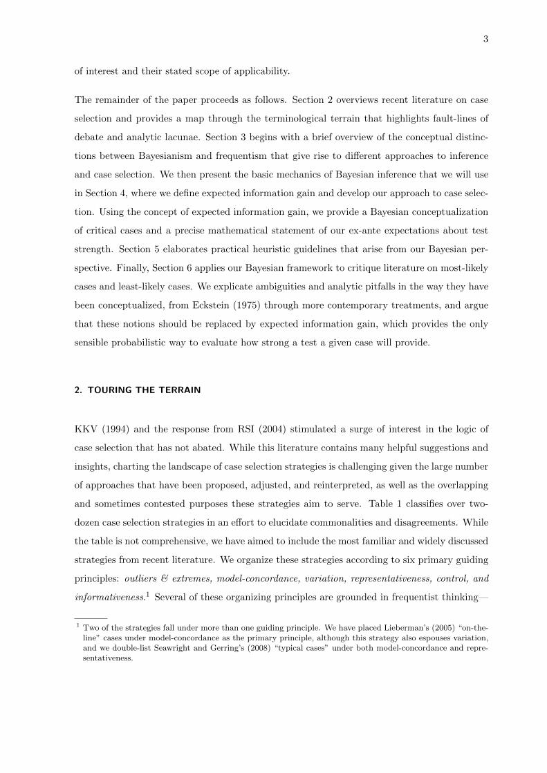
odds-ratio form of Bayes’ rule:

posterior odds = prior odds ⇥ likelihood ratio

P (Hi |E I)P (Hj |E I) =

P (Hi | I)P (Hj | I) ⇥ P (E |Hi I)

P (E |Hj I) ,(1)

The posterior odds on the left-hand side of equation (1) tell us how much more plausible one

hypothesis Hi is relative to a rival hypothesis Hj in light of the evidence learned as well as the

background information we initially brought to the problem, while the prior odds on the right-

hand side is the plausibility of Hi compared to Hj based only on our background information.

For posterior odds and prior odds, we can think in terms of how willing we would be to bet

in favor of one hypothesis vs. the other. The likelihood ratio7—the second factor on the right-

hand side of (1)—represents how plausible, or expected, the evidence is under one hypothesis

relative to the other, or in other words, how likely the evidence would be if we assume Hi is

true, compared to how likely the evidence would be if we instead assume Hj is true. According

to Bayes’ rule, how much we end up favoring one hypothesis over another depends on both our

prior views and the extent to which the evidence weighs in favor of one hypothesis over another.

Assessing likelihood ratios P (E |Hi I)/P (E |Hj I) is therefore the critical inferential step that

tells us whether evidence E should make us more or less confident than we were initially in

one hypothesis relative to a rival. The likelihood ratio can be thought of as the probability of

observing E in a hypothetical world where Hi is true, relative to the probability of observing E

6 As we elaborate elsewhere, it is always possible to begin with a set of causal factors or causal hypothesesthat are non-rival and create from them a set of hypotheses that are mutually exclusive (Fairfield & Charman2017).

7 What we call the likelihood ratio is sometimes referred to as the Bayes factor.

10

in an alternative world where Hj is true. When evaluating likelihoods of the form P (E |Hi I),we must in e↵ect (a) suppress our awareness that E is a known fact, and (b) suppose that

Hi is correct, even though the actual status of the hypothesis is uncertain. Recall that in the

notation of conditional probability, everything that appears to the right of the vertical bar is

either known, or assumed as a matter of conjecture when reasoning about the probability of

the proposition to the left of the bar. In qualitative research, we need to “mentally inhabit the

world” of each hypothesis (Hunter 1984) and ask how surprising (low probability) or expected

(high probability) the evidence E would be in each respective world. If E seems less surprising

in the “Hi world” relative to the “Hj world,” then that evidence increases our odds on Hi vs.

Hj . Again, we gain confidence in a given hypothesis to the extent that it makes the evidence

we observe more plausible compared to rivals.

3.3. Example: State-Building in Latin America

To illustrate how Bayesian reasoning can be applied in qualitative social science, suppose we

are interested in whether the resource-curse hypothesis, or the warfare hypothesis (assumed

mutually exclusive), provides a better explanation for institutional under-development:

HR = Mineral resource dependence is the central factor hindering institutional development

in Latin America. Mineral wealth makes collecting taxes irrelevant and creates incentives for

subsidies and patronage, instead of building administrative capacity.

HW = Absence of warfare is the central factor hindering institutional development in Latin

America. Without external threats that necessitate e↵ective military defense, leaders lack in-

centives to collect taxes and build administrative capacity.

For simplicity, suppose we have no relevant background knowledge about state-building. We

would then reasonably assign even prior odds, such that our log-odds will equal one. We now

learn the following information about Peru:

E1 = Peru faced persistent military threats following independence, its economy was long

dominated by mineral exports, and it never developed an e↵ective state.

Intuitively, E1 strongly favors the resource-curse hypothesis. Applying Bayesian reasoning, we

must evaluate the likelihood ratio P (E1 |HR I)/P (E1 |HW I). Imagining a world where HR is

11

the correct hypothesis, mineral dependence in conjunction with weak state capacity is exactly

what we would expect, and external threats are not surprising given that a weak state with

mineral resources could be an easy and attractive target for invasion. In the alternative world

of HW , E1 would be quite surprising; something very unusual, and hence improbable, must

have happened for Peru to end up with a weak state if the warfare hypothesis is nevertheless

correct, because weak state capacity despite military threats contradicts the expectations of the

theory. Because E1 is much more probable under HR relative to HW—that is, P (E1 |HR I) ismuch greater than P (E1 |HW I)—the likelihood ratio is large, and it significantly boosts our

confidence in the resource-curse hypothesis.

Our posterior log-odds in light of E1, which now strongly favor HR over HW , in turn become

our prior log-odds when we move forward to consider an additional evidentiary observation

E2. Updating proceeds iteratively is this manner until we decide to terminate our research and

report our findings, or until a new or refined hypothesis comes to light. In the later situation,

we would need to go back and set up a di↵erent inferential problem that compares the revised

set of hypotheses in light of our background information and all of the evidence obtained thus

far.

3.4. Bayes’ Rule in Log-Odds Form

If we take the logarithm of both side of Bayes’ rule (1), we obtain a particularly simple, additive

relationship that is easy to remember and easy to use:

logh P (Hj |E I)P (Hk |E I)

i= log

h P (Hj | I)P (Hk | I)

P (E |Hj I)P (E |Hk I)

i

= logh P (Hj | I)P (Hk | I)

i+ log

h P (E |Hj I)P (E |Hk I)

i

posterior log-odds = prior log-odds + weight of evidence ,

(2)

where we have used the fundamental property that the logarithm of a product equals the sum

of the logarithms. The weight of evidence (Good 1983), which is just the the logarithm of the

likelihood ratio, conveys the probative value of the evidence—namely, how much it supports

one hypothesis compared to another (setting aside our prior beliefs about the hypotheses). We

will denote the weight of evidence in favor of hypothesis Hj relative to hypothesis Hk as:

WoE (Hj : Hk) = logh P (E |Hj I)P (E |Hk I)

i. (3)

12

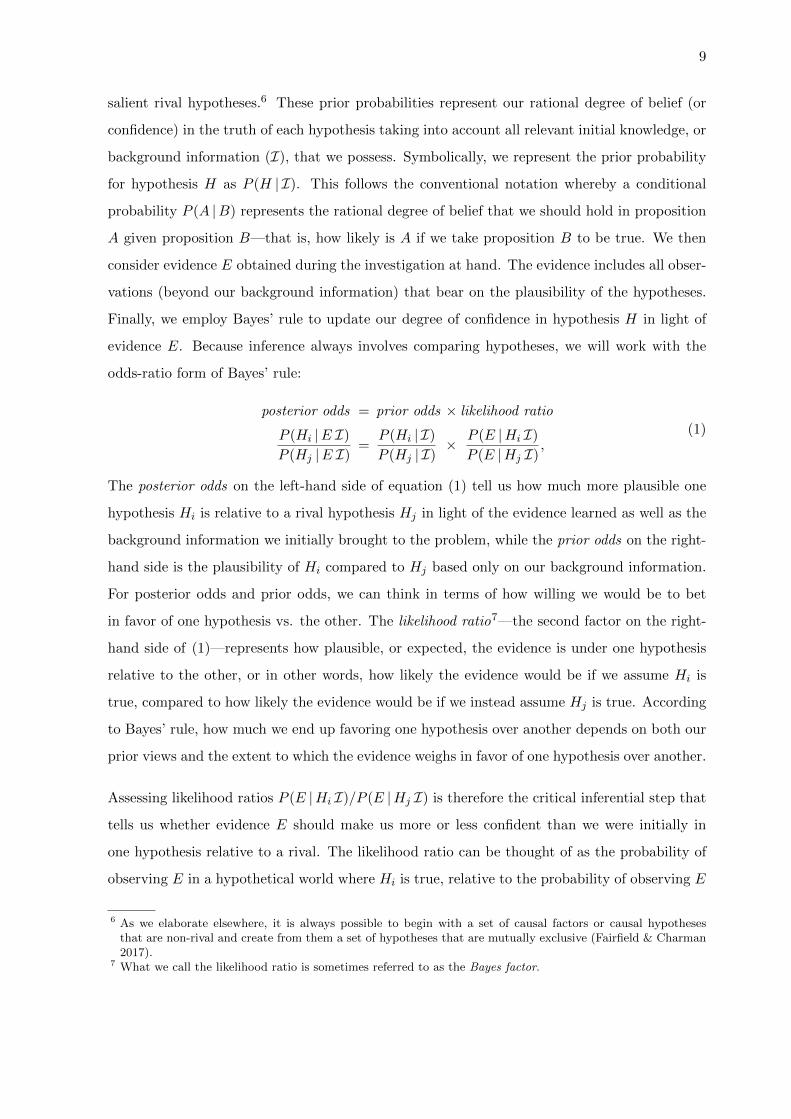
As the term suggests, the weight of evidence is additive. In particular, when the aggregate

or total evidence E can be decomposed into a conjunction of separate pieces, such that E =

(E1E2 · · ·EN ), the overall or net weight of evidence (3) can itself be broken down into the sum

of weights for each distinct piece of evidence:

WoE (Hj : Hk) = logh P (EN |E1E2 · · ·EN�1Hj I)P (EN |E1E2 · · ·EN�1Hk I) · · ·

P (E2 |E1Hj I)P (E2 |E1Hk I)

P (E1 |Hj I)P (E1 |Hk I)

i

= logh P (EN |E1E2 · · ·EN�1Hj I)P (EN |E1E2 · · ·EN�1Hk I)

i+ log

h P (E2 |E1Hj I)P (E2 |E1Hk I)

i+ log

h P (E1 |Hj I)P (E1 |Hk I)

i

= WoEN (Hj : Hk , E1 · · ·EN�1) + · · ·+WoE2 (Hj : Hk , E1) +WoE1 (Hj : Hk) ,

(4)

where our notation denotes that for each successive piece of evidence we must take into ac-

count possible logical dependencies with previously-analyzed evidence, a task that we discuss

elsewhere (Fairfield & Charman 2017).8

Beyond the simplicity of equation (2) and the additivity of weights of evidence, there are deeper

reasons for using logarithms. As explained in Fairfield & Charman (2017), a logarithmic scale

allows us to better handle very large or very small probabilities and a↵ords better consistency

with human sensory perception, when compared to a linear scale.

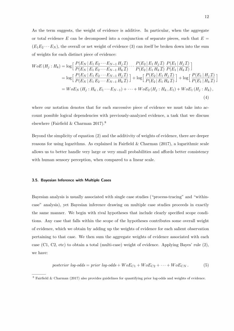
3.5. Bayesian Inference with Multiple Cases

Bayesian analysis is usually associated with single case studies (“process-tracing” and “within-

case” analysis), yet Bayesian inference drawing on multiple case studies proceeds in exactly

the same manner. We begin with rival hypotheses that include clearly specified scope condi-

tions. Any case that falls within the scope of the hypotheses contributes some overall weight

of evidence, which we obtain by adding up the weights of evidence for each salient observation

pertaining to that case. We then sum the aggregate weights of evidence associated with each

case (C1, C2, etc) to obtain a total (multi-case) weight of evidence. Applying Bayes’ rule (2),

we have:

posterior log-odds = prior log-odds+WoEC1 +WoEC2 + · · ·+WoECN . (5)

8 Fairfield & Charman (2017) also provides guidelines for quantifying prior log-odds and weights of evidence.

13

To the extent that the N cases already studied increase our confidence in the truth of one

hypothesis relative to rivals, as reflected in our posterior log-odds, we become more confident

that this hypothesis successfully explains other, as-yet unobserved cases that fall within its

scope. This is an iterative process, where we can always add additional cases and revise theory

and scope conditions.

Returning to the state-building example, notice first that the two hypotheses we considered

include scope conditions that restrict their predictions to Latin American countries—in other

words, these hypotheses say nothing at all about institutional under-development in, for ex-

ample, Eastern Europe. Suppose a thorough investigation of the Peruvian case yields a weight

of evidence WoEP in favor of HR over HW . We then proceed to analyze the Venezuelan case

and obtain a weight of evidence of WoEV in favor of HR over HW . Starting from even prior

odds, our posterior log-odds then favor HR by an amount (WoEP + WoEV ), which we will

assume for illustration corresponds to a very strong degree of confidence in the resource-curse

relative to the warfare hypothesis. Moving forward, we accordingly have a very strong degree

of confidence that the resource curse will explain institutional under-development better than

the warfare hypothesis for any other Latin American case. Of course, we are conducting prob-

abilistic inference with incomplete information, so we might discover evidence in another case

that leads us to revise our views about these hypotheses.

If we wish to generalize our hypotheses beyond Latin America, we begin by articulating revised

versions with broader scope conditions; for example:

H 0R = Mineral resource dependence is the central factor hindering institutional development

in the global south. Mineral wealth makes collecting taxes irrelevant and creates incentives for

subsidies and patronage, instead of building administrative capacity.

H 0W = Absence of warfare is the central factor hindering institutional development in the

global south. Without external threats that necessitate e↵ective military defense, leaders lack

incentives to collect taxes and build administrative capacity.

Because Peru and Venezuela also fall within the scope of these generalized hypotheses, our

previous study of these two cases give us a very strong degree of confidence in H 0R vs. H 0

W , just

as these cases led us to very strongly favor HR over HW . But as a next step, we would want

to examine cases from another developing region—perhaps India or Egypt. While studying

14

additional Latin American cases will contribute to our inference, seeking cases from other

developing regions will be the most e↵ective way to assess how well H 0R fares against H 0

W .

4. OPTIMAL BAYESIAN CASE SELECTION

Logical Bayesianism provides a comprehensive, information-theoretic approach to choosing

cases for hypothesis testing. In principle, the single overarching case-selection criterion should

entail maximizing anticipated informativeness; the more we expect to learn, the more “criti-

cal,” or inferentially decisive, the case becomes. More precisely, we seek cases that maximize

expected information gain—the anticipated weight of evidence in favor of whichever hypothesis

under consideration provides the best explanation. We begin with a general introduction to the

information-theoretic approach, where we invoke an analogy to e�cient questioning. Readers

who prefer to skip mathematical details may proceed directly from this introduction to Section

4.4, where we present some practical caveats and principled insights, given that in practice,

calculating expected information gain in anything but a very rough approximation generally

will not be feasible.

4.1. Introduction to the Information-Theoretic Perspective

Logical Bayesianism is closely connected to information theory, which provides a framework for

e�cient questioning. The idea is to figure out which cases we should select in order to adjudicate

between rival hypotheses as quickly as possible. We can think of experimentation or observation

as communication with the physical or social world; the observable features of the world are

messages transmitted—usually with noise—to the researcher, who endeavors to decode the

signals. The simplest scenarios involve hypotheses that make deterministic predictions, and

observations with negligible measurement error that reveal one among a finite number of possible

evidentiary outcomes. The real world is rarely so straightforward, but such scenarios illustrate

some of the salient issues that arise in case selection and suggest some general strategies.

Consider first the classic game of “twenty questions,” where we ask a series of yes-or-no queries

to figure out what subject a friend has in mind. Here we have an essentially infinite number of

possible hypotheses as to what the subject may be, with evidentiary outcomes that entail either

15

a “yes” or a “no” answer. To e�ciently reduce uncertainty, instead of asking questions designed

to eliminate one specific possibility at a time (e.g., Barak Obama, duck-billed platypus, earl-grey

gelato) we should aim to ask questions that halve the remaining possible hypotheses at each

stage (e.g., something like: “is or was the subject a living organism?”). This strategy may not

be optimally informative with respect to any one hypothesis, but this approach is optimal for

winnowing down sets of hypotheses. Likewise, optimal case selection should not be conducted

with a single hypothesis in mind, but instead with the aim of e�ciently distinguishing between

salient rival explanations.

As a second example, consider Wason’s (1968) “selection task,” or four-card problem, which

in contrast to “twenty questions” involves a finite number of hypotheses, as well as a finite

number of noiseless evidentiary outcomes. Four cards are displayed on a table, as in Figure

1. We know that each card has a number on one side, and a color on the other side that can

be either red or blue. We are given a hypothesis about the relationship between numbers and

colors on the cards: H = If a card has an even number on one face, its opposite face must be

red. Given what we observe on the table—a 3, a blue face, an 8, and a red face, which card(s)

should we turn over to definitively test whether this hypothesis is true or false? The goal is to

flip as many cards as needed to be sure, but no more.

Here is an ex: suppose we have four cards, and we know that each of them has a

nmbr on one side and a color on the other side—either R or B.

We have a H about the relationship btwn nmbrs and colors on the cards—the

proposition is that if a card has an EVEN nmbr on one face, its op face is RED.

Given these four cards, which ones shld you turn over to test wthr this H is T or F?

Take a couple minutes to think about it, and then we’ll do a poll. [HANDOUT, START TP][email protected], psw: Peppercorn7

[Answer: 8-card AND blue card.]

19

FIG. 1 Wason’s (1968) “selection task”

To solve the problem, first notice that H = It is not the case that if a card has an even number

on one face, its opposite face must be red, logically implies the proposition: There is at least one

even card that is blue on the other side. Accordingly, we need to turn over the 8 and check its

color. If this card is blue, then H is false and we are done. If it is instead red, then H becomes

more plausible, but we need to turn over another card before we can can reach a definitive

conclusion. The second card that we need to check is that with the blue face. If it has an even

number on the other side, then H is false. If it instead has an odd number, then H is true

(assuming that the 8 card turned out to be red on its other face). It does not matter whether

we flip the blue card or the 8 card first. The important point is that these are the two cards

16

that will provide useful information for figuring out whether the hypothesis is true or false.

Nothing is learned by flipping the 3, because neither H nor H says anything about what color

we should expect to find on the back of an odd card. We are also wasting time and e↵ort if we

flip the red card, because both possible outcomes (odd or even) are equally consistent with H

and H—notice that H only tells us what to expect if we know one side to be even; it does not

tell us what we should find on the opposite side of a red card.

The four-card problem provides an analogy for purposive sampling, where we make decisions

about which cases (cards in this instance) to investigate based on the hypotheses under consid-

eration and the information we are likely to learn, rather than selecting at random. Moreover,

this example illustrates that random sampling—the guiding principle within frequentism—can

actually be a sub-optimal strategy for case selection. If we were to randomly choose two cards

to flip, the probability of drawing the blue card and the 8 card—the only two cards that provide

useful information for assessing the hypotheses—is only 1/6. It turns out that in many situa-

tions, random sampling is sub-optimal—we can do better by employing an information-theoretic

approach that directs us to identify cases with maximum informativeness.

Wason’s (1960) “sequence task” provides a third example, involving the following setup. We

are asked to infer a particular rule (determined by the experimenter) that is used to generate

sequences of three integers. We are given one instance of a sequence satisfying the rule (e.g.,

2, 4, 6). We can then propose additional three-number sequences as test cases and will be told

whether or not each such test sequence satisfies the rule. This example is an analogue for infer-

ence involving an infinite number of potential “cases” with which to assess an infinite number

of possible hypotheses, none of which can be definitively confirmed.9 While the sequence task

might more naturally serve as an analogy for experimental rather than observational research,

since we generate the “cases” ourselves, some useful insights for case selection nevertheless

emerge from this problem.

Given the goal of e�ciently narrowing down the field of candidate hypotheses with as few

test sequences as possible (i.e., examining as few cases as possible), choosing at random would

once again be suboptimal—in fact, that approach would be about the most ine�cient strategy

9 In the original experiment, Wason (1960:131) told participants: “When you feel highly confident that you havediscovered it [the rule], and not before, you are to write it down and tell me what it is.” If the proposed rule wascorrect, the experiment ended, so in this sense the participants hypothesis was confirmed in practice. OtherwiseWason (1960:132) allowed the participant to continue inventing hypotheses and proposing test sequences.

17

imaginable. Proposing trial sequences that conform to a pet hypothesis is also suboptimal.

Wason (1960) observed that many participants followed this kind of approach and succumbed

to confirmation bias—they became too confident too quickly in incorrect, often overly-complex

rules. A Popperian perspective would suggest that we should aim to falsify hypotheses rather

than confirm them. But that approach would also be ine�cient, just as eliminating possibilities

one by one in the twenty-questions game is ine�cient.

From a Bayesian or information-theoretic perspective, we should try to choose the test cases

that discriminate most e↵ectively between rival hypotheses. A natural strategy for the sequence

task entails generating an initial set of ten or so reasonably plausible hypotheses (based per-

haps on an assumption that if the rule were too complicated, the experimenter would have

trouble judging in a timely manner whether proposed trial sequences obeyed it or not), orga-

nizing them into families or classes by identifying more general hypotheses and sub-hypotheses

that are more specific or more restricted instances thereof, and then choosing test cases that

di↵erentiate between classes of hypotheses. This approach helps eliminate multiple candidate

rules with a single test case, regardless of whether we discover that our test sequence fits or

violates the experimenter’s rule. For example, if we learn that (6, 4, 2) does not fit, we can elim-

inate hypotheses postulating “all triples of integers,” “all even integers,” and “all arithmetic

sequences”10 along with more restricted hypotheses that fall within that class (e.g., “sequences

where each integer di↵ers by ±2 from its predecessor”). If we instead learn that (6, 4, 2) sat-

isfies the sequence-generation rule, we can eliminate hypotheses postulating “three increasing

integers” and any more specific variants thereof (e.g., “sequences where each integer di↵ers by

+2 from its predecessor”), and so forth. If none of our initial hypotheses survive after propos-

ing several test sequences, we can go back, invent more possibilities, and repeat this process.

Likewise, case selection in social science can be an iterative process that proceeds alongside

theory development.

In sum, an information-theoretic perspective reveals that (i) random selection is generally not an

optimal strategy for case selection,11 and (ii) cases should not be chosen in an e↵ort to confirm

a given hypothesis, nor to submit a single hypothesis to repeated attempts at falsification.

10 Such sequences are characterized by a constant di↵erence between consecutive terms.11 Jaynes (2003:532), an outspoken advocate of logical Bayesianism in the physical sciences, asserts much more

generally that: “Whenever there is a randomized way of doing something, there is a nonrandomized way thatyields better results from the same data, but requires more thinking.”

18

Instead, we should aim to examine cases for which rival hypotheses, or sets of rival hypotheses,

make the most divergent evidentiary predictions, or in other words, those cases we expect to be

most informative. In Bayesian terms, we want to choose cases that we anticipate will provide

a large weight of evidence—the quantity in Bayes’ rule that governs updating.

4.2. Discrimination Information

The first step toward quantifying anticipated informativeness entails recognizing that we cannot

know for certain what evidence we will discover before we actually investigate a given case C. At

least in principle, however, we could use our background information to anticipate the di↵erent

sorts and combinations of clues we might find, estimate their respective weights of evidence for

the hypotheses that we are considering, and then average over all of the anticipated evidentiary

possibilities.

Proceeding formally, we begin with the assumption (included in the background information I)that we have a finite, mutually-exclusive and exhaustive set of hypotheses {Hj}.12 The logical

negation of any one of the hypotheses is then the disjunction over the remaining alternatives:

H j =_

6=j

H` = H1 or · · · Hj�1 orHj+1 or · · ·HN . (6)

We also assume that we have delineated a complete and mutually exclusive set of possible

evidentiary outcomes for the case, {Ek}. Each possible Ek represents the composite information

that could be learned from the case, given a research strategy SC . To illustrate with a simple

example, suppose our cases are democratic countries and our data gathering strategy (SC)

entails soliciting interviews with the president and the opposition leader and asking each a

specific yes/no question. One possible evidentiary outcome would be E1 = President says yes

and opposition says no. A second outcome could be E2 = President could not be interviewed and

opposition says no. Assuming that each of the two informants is associated with three possible

“clue outcomes” (yes, no, or could not be interviewed), we would have a set of 3⇥3 = 9 possible

evidentiary outcomes Ek. (In real-world case studies, the possible set of evidentiary outcomes

will of course be vastly larger.)

12 The assumption of exhaustivenes is necessary for posing a well-specified inferential problem (Jaynes 2003). Ifa new hypothesis comes to mind in the future, we simply start over with a new, expanded or revised set ofhypotheses that we provisionally consider to be exhaustive. Bayesian inference is always tentative inference tothe best existing explanation.

19

The discrimination information D(Hj : H j |SC Hj I) also known as the relative entropy, quan-

tifies the expected weight of case evidence in favor of Hj relative to H j when we assume that

Hj is in fact true:

D(Hj : H j |SC Hj I) =X

k

P (Ek |SC Hj I) loghP (Ek |SC Hj I)P (Ek |SC H j I)

i. (7)

In other words, expression (7) averages the possible weights of evidence (the log of the likelihood

ratio), each weighted by its respective likelihood under Hj .13

The Gibbs inequality (a mathematical theorem from statistical mechanics) guarantees that the

discrimination information is nonnegative:

D(Hj : H j |SC Hj I) � 0, (8)

with equality if and only if P (Ek |SC Hj I) = P (Ek |SC H j I) for every possible evidentiary

outcome Ek. This latter situation would mean that we cannot learn anything about the truth

of Hj from the case, which would seem to be extremely rare in practice. Aside from such

special situations, we have the nontrivial fact that, on average, we always expect to find evi-

dence favoring a hypothesis, assuming that it is indeed true. This expectation must hold for

every hypothesis, even though: (i) for any given hypothesis, some of the possible clues must

produce non-negative weights of evidence while others must yield non-positive weights of evi-

dence (because a hypothesis cannot be confirmed by all possible evidence—otherwise we could

boost its credence without bothering to actually gather any evidence from the case); and (ii),

any given clue must be associated with non-negative weights of evidence for some hypotheses

and non-positive weights for others (the same evidence cannot boost the plausibility of ev-

ery hypothesis, otherwise the sum of their probabilities would exceed unity). Small values of

D(Hj : H j |SC Hj I) suggest that the case is expected to be uninformative about Hj if that

hypothesis is true, in the sense that Hj does not tend to make sharp predictions for this case

that di↵er from those predicted by its plausible rivals. A large value of D(Hj : H j |SC Hj I)instead predicts that if Hj is in fact true, the case will provide strong evidence supporting

this conclusion. In other words, small values of D(Hj : H j |SC Hj I) indicate that the case

prospectively provides a weak test for Hj , while large values indicate that the case constitutes

a prospectively strong test for Hj .

13 Although not manifest, the generalized discrimination information implicitly (and inconveniently) depends onthe priors P (Hj | I).

20

We can also construct the “dual” discrimination information for H j versus Hj ,

D(H j : Hj |SC H j I) =X

k

P (Ek |SC H j I) loghP (Ek |SC H j I)P (Ek |SC Hj I)

i, (9)

which likewise satisfies the Gibbs inequality:

D(H j : Hj |SC H j I) � 0 , (10)

with equality if and only if P (Ek |SC Hj I) = P (Ek |SC H j I) for all possible observational

outcomes. This inequality ensures that if Hj is assumed false (i.e., one of the concrete rival

hypotheses postulated under I is true instead, but we do not know which), then we expect to

find some evidence tending to disconfirm Hj . A low value for D(H j : Hj |SC H j I) indicates

that the case is expected to be uninformative when Hj is false, whereas a high value indicates

that the case is expected to strongly disconfirm Hj if it is false.

If we single out a particular hypothesis of primary interest, we can make a formal correspon-

dence between discrimination information and a generalized version of Van Evera’s (1997) test

typology that allows for non-binary evidentiary outcomes (Figure 2). Large values for both the

discrimination information D(Hj : H j |SC Hj I) and its dual D(H j : Hj |SC H j I) indicate a

prospective doubly-decisive case, where we expect to learn a lot about the truth of Hj regardless

of which clues we eventually discover. In contrast, small values of both D(Hj : H j |SC Hj I)and D(H j : Hj |SC H j I) indicate a prospective straw-in-the-wind case, which we expect to

provide little information about the truth of Hj .

Mismatches between the discrimination information and its dual yield Van Evera’s other two

test types. A large value of D(Hj : H j |SC Hj I) and small value of D(H j : Hj |SC H j I)corresponds to a prospective smoking-gun case for Hj (or equivalently, a hoop case for H j).

Conversely, a small value of D(Hj : H j |SC Hj I) and large value of D(H j : Hj |SC H j I)indicates a prospective hoop test for Hj (or equivalently, a smoking-gun test for H j). It is

important to emphasize that characterizing a case prospectively as a smoking-gun test does not

imply that we have a strong expectation of finding smoking-gun evidence upon studying that

case. On the contrary, in a smoking-gun test, it is much more likely that we will not actually

find the smoking gun. However, the case provides the potential for a large weight of evidence

in favor of Hj , if the smoking-gun evidence is indeed observed.

When working with prospective Van Evera test types for case selection, we must keep three

critical points in mind. First, the posterior informativeness of a case study for Hj vs. H j , based

21

2"D (H0 ; H1)

D (H

1 ; H

0)

Smoking gun for H1 or Hoop test for H0

Smoking gun for H0 or Hoop test for H1

Doubly decisive

Straw in the wind

FIG. 2 Prospective Van Evera case types classified in terms of discrimination information for a set of

binary MEE hypotheses

on the actual observations we make, may be higher or lower than the prior expectation. Second,

a case may be more or less informative (in either prospective expectation or retrospective

actuality) for adjudicating between some other hypothesis Hk 6=j and its negation. This latter

point is particularly salient for prospective straw-in-the-wind cases. We might not want to

discard studying such cases before considering whether we stand to learn substantial information

about the truth of one of the other plausible rival hypotheses Hk for k 6= j. Third, we emphasize

again that from a Bayesian perspective, the goal is not to try to confirm or falsify a single

hypothesis of interest Hj , but rather to adjudicate between all plausible rival hypotheses.

4.3. Expected Information Gain

Given that we do not know which of the hypotheses under consideration is correct, a better

approach to case selection involves averaging the expected weight of case evidence, D(Hj :

H j |SC Hj I), over all of the hypotheses, each weighted by its respective prior probability. The

22

resulting expression is the expected information gain associated with case C:

D(SC, I) =X

j

P (Hj | I)D(Hj : H j |SC I)

=X

j

P (Hj | I)X

k

P (Ek |Hj SC I) loghP (Ek |SC Hj I)P (Ek |SC H j I)

i

=X

j

P (Hj | I)X

k

P (Ek |Hj SC I)WoE (Hj : H j , SC) .

(11)

In essence, the expected information gain D averages the weight of evidence over our uncertainty

about what clues we will discover (as represented by the likelihoods for Ek), and (ii) our

uncertainty regarding which hypothesis is correct (as represented by the prior probabilities).

In plain language, expected information gain is the anticipated weight of evidence in favor of

whichever hypothesis is true.

Invoking the Gibbs inequality as before, expected information gain must be nonnegative:

D(SC, I) � 0, (12)

and can vanish if and only if P (Ek |SC Hj I) = P (Ek |SC H j I) for all evidentiary outcomes and

all hypotheses under consideration. For any given case, there is of course no guarantee that the

evidence uncovered will point toward the true hypotheses; case evidence might be misleading.

However, on average (i.e., across all plausible Hj and potential Ek), any case is expected to

provide evidentiary weight in favor of the true hypothesis.

4.4. Practical Caveats and Principled Insights

The good news is that maximizing expected information gain, D(SC, I), provides a cogent,

mathematically-grounded principle to guide case selection for theory testing. Recall that this

quantity (equation 11) represents the anticipated weight of evidence in favor of the true hypoth-

esis, which we obtain by averaging the weight of evidence over all possible evidentiary outcomes

for the case, weighted by the respective likelihoods, and then average over all of the plausible

hypotheses, weighted by the respective prior probabilities.

The bad news is that prospects for prospectively calculating anything but a very rough approxi-

mation to D(SC, I) are daunting—we would have to assess likelihoods for all possible evidence in

the cases under consideration. We do have some freedom in deciding how to partition the space

23

of possible observations, so we could try to work with a relatively course level of granularity

in order to contain the total number of distinct possible outcomes we must consider. However,

as discussed in Fairfield & Charman (2019), it is not unusual for the likelihoods of case-based

evidence to depend on subtle details of phrasing, timing, body language of informants, etc.

The power of evidence to discriminate between hypotheses might very well lie in features that

cannot easily be foreseen. We therefore face a formidable tradeo↵: if we adopt too fine-grained

a partition, tracking and assessing all of the possible observations becomes cumbersome, ine�-

cient, and ultimately unattainable given the impossibility of anticipating all salient details that

could arise. If we make do with too course a partition, the evidentiary possibilities we consider

will be too vague and insu�cient for (or ine�cient at) adjudicating between hypotheses.

Another di�culty with trying to calculate expected information gain is that likelihoods depend

critically on the search strategy we following for finding evidence in the case. In line with

the analogy of Bayesian inference as a dialogue with the data, the actual manner in which we

gather evidence within a case typically is not pre-determined; instead, it is a highly dynamic

and interactive process that is contingent on evidence gathered previously. Recall that the case

evidence Ej will typically consist of the conjunction of multiple observations or clues such that:

P (Ej |SC H I) = P (Ej1Ej2 · · · |SC H I)= P (Ej1 |SC H I)P (Ej2 |Ej1SC H I)P (Ej3 |Ej2Ej1SC H I) · · · .

(13)

Any real-world search strategy SC may become highly complex, since particular clues may

prompt follow-up questions and e↵orts to dig deeper that may direct us to pursue certain sources

more diligently or even to discover sources we were not aware of previously. Given unforeseeable

contingencies, it will be prohibitively di�cult to spell out SC explicitly in advance for all forks

in the investigative path—the tree of possibilities will be too intricate and profuse.14 Even if

one could foresee all possibilities, there will be too many to analyze in any detail in advance.

By contrast, whereas D depends on likelihoods, Bayesian updating once the evidence is in hand

depends only on likelihood ratios, P (Ej |SC H1 I)/P (Ej |SC H2 I), which makes conditioning

on the search strategy largely irrelevant. Whatever search strategy ultimately produced the

evidence, and however likely or unlikely we were to obtain that evidence, post-facto, the di↵er-

ence in likelihoods depends only on which hypothesis we condition on. Accordingly, post-data

14 Nevertheless, despite appearances, our formal notation does at least allow for such highly contingent or path-dependent search strategies—the problem is simply that of prospectively specifying SC.

24

inference is a far simpler task than prospectively calculating expected information gain. To

illustrate, suppose that our research involves interviewing politicians to find out why a tax cut

was enacted. The search strategy entails working hard to gain access to members of parliament.

But it is so unlikely from the outset that we would be able to interview the prime minister that

we do not plan to invest much e↵ort to that end. If Ek represents some kind of information we

could imagine receiving from an interview with the prime minister, Ek will contribute negligi-

bly to expected information gain, simply because the likelihood of obtaining any information

directly from the prime minister is so low. But now suppose that once in the field, by a stroke

of luck we meet the prime minister’s top aid, who then arranges a brief interview with the

prime minister. Post facto, how likely it was that we would be able to access the prime min-

ister is irrelevant, because obtaining access was essentially equally unlikely regardless of which

hypothesis provides the best explanation for the tax cut.

As a normative goal or prescriptive ideal, logical Bayesianism ignores the di�culty of calculating

quantities such as expected information gain; it presumes a sort of “logical omniscience,” where

the implications of propositions are presumed immediately known, and the temporal or eco-

nomic costs of information acquisition and information processing are largely ignored. At best,

we can aspire to approximate this ideal, taking practical limitations into account. For example,

it can be tedious to carry forward many di↵erent rival hypotheses, so instead of maximizing

expected information gain overall, it might make sense to try to find a “nail-in-the-co�n” case

for one or more of the least plausible hypotheses, which might then lose enough credence to be

e↵ectively removed from serious consideration.

Yet however di�cult to quantify in practice, expected information gain does tells us in principle

what we should look for in a case that is intended to test theory. From a Bayesian perspective,

the goal is not to try to confirm a primary hypothesis a la Hempel, nor to create an opportunity

for falsifying this hypotheses a la Popper, but to distinguish between alternative hypotheses,

considered on equal footing.

Our formal discussion of expected information gain fortifies this common-sense advice and

allows us to end on a highly encouraging note. If we wish to reduce our uncertainty over a set

of hypotheses, or to gain credence in the true hypothesis, then prospectively, we always expect

to learn from studying any given case. In that sense, there are no bad cases, just varying degrees

of better cases. Therefore, all is not lost if we end up (unknowingly) choosing sub-optimal cases;

25

a priori we can still expect the case study to contribute something to knowledge accumulation.

5. HEURISTIC BAYESIAN CASE SELECTION

In light of the obstacles facing e↵orts to perform truly optimized case selection, this section

o↵ers practical, Bayesian-inspired advice and considers how this advice either di↵ers from or

helps substantiate prevailing recommendations in the literature. While some of our suggestions

clearly break with extant views, many are matters of common sense and/or correspond to well-

established practices in qualitative research. Regarding the latter category, our goal in large

measure is precisely to show that Bayesianism justifies and underpins many widespread practices

that most scholars would probably consider intuitively reasonable, but without necessarily being

able to provide a consistent or coherent rationale as to why.

5.1. If substantial knowledge is available prior to case selection, aim to choose cases that

maximize some approximation to, or proxy for, expected information gain. If less is known about

potential cases a priori, seek cases that are anticipated to be data rich. If even less is known,

prioritize practical concerns and curtail e↵ort spent on case selection.

As elaborated in Section 4, we should aim to choose the cases that will be most informa-

tive; however, very often we will not have enough knowledge or resources ahead of time to

be able to make anything resembling a mathematically optimal choice a priori. For example,

as discussed in Section 2, much of the literature assumes that scores on key independent and

dependent variables are known in advance of case selection, yet for many innovative qualitative

research projects, this information itself is often produced only during the course of in-depth

case research. In such situations, we advocate prioritizing practical concerns and moving on

to in-depth data collection. Among other factors, salient practical concerns include language

skills, safety of the research venue, quality of secondary sources, access to archives and relevant

documentation, accessibility of key informants, and budget or time constraints.

26

5.2. There is no need to list all known cases before choosing some for in-depth investigation.

The near-universally espoused advice to begin the case selection process by enumerating all

possible cases is grounded in a frequentist approach to inference, where the population and

the procedure for sampling from that population must be fully specified before data collection

and analysis. From a Bayesian perspective, however, we regard this advice as misguided and

unnecessary. Qualitative research generally does not (and quite possibly cannot) aspire to

estimate numerical values for population-level parameters; as such, case selection does not

require randomly sampling from a pre-defined population, and in this sense at least, selection

bias cannot be an issue. Moreover, providing readers with a list of cases that were not chosen

for close analysis provides no salient information for evaluating inferences drawn from the

cases that actually were studied. In contrast to frequentism, where inference is always based

on considerations of what would happen under (often only imagined) repetitions of the same

sampling procedure, cases (or data) that were not investigated (or not obtained) play no direct

role in Bayesian analysis. Within a Bayesian framework, we are concerned with (1) conducting

sound inferences based on the actual evidence at hand—without ignoring salient information

and without allowing subjective hopes or counterfactual speculations to a↵ect our analysis—and

(2) articulating scope conditions in a manner that attempts to balance explanatory power and

generality—or stated di↵erently, accuracy and simplicity.15 If scholars are concerned that the

studied cases are unusual or misleading, such that the theoretical argument would not fare well

against rivals if the breadth of analysis were expanded, then follow-up research to strengthen

inferences can be conducted on additional cases within the original scope of the theory, and/or

extensions of the research can be carried out to assess and refine the theory in new contexts

that push the boundaries of the original scope conditions.16

Our Bayesian perspective is particularly salient considering that delineating the entire popula-

tion of applicable cases ahead of time would often be prohibitively di�cult. Because Bayesian

analysis invites an iterative dialog with the data where we may generate and refine hypotheses

and scope conditions as we gather new information, we are free to add cases as our research

progresses. In many situations, new cases will be constantly generated over time; consider

15 To that end, Bayesianism automatically incorporates an “Occam razor” that penalizes complexity beyondwhat is needed to explain the data (Fairfield & Charman 2019).

16 See Fairfield & Charman (2020) for discussion of continued research and extended research in the context ofdebates on replication and reliability of inference.

27

for example research on policy initiatives (e.g., tax reform or social policy innovation), elec-

toral campaigns, populist leaders, or transitions between democratic and authoritarian regimes.

When case selection follows a multi-level process (e.g., choosing countries and then identifying

salient reform episodes, court cases, or protest events within those countries), ongoing fieldwork

may be necessary to discover relevant cases within the macroscopic unit; information may not

be available outside of the country to identify salient cases in advance of consulting primary

documents or interviewing local experts.17

While Bayesian case selection need not begin with a fully enumerated population, it can cer-

tainly be useful to list a number of salient cases from the outset. At early stages of research,

considering preliminary information known about a substantial range of cases can stimulate

ideas about plausible hypotheses and scope conditions. In addition, we will argue that includ-

ing diverse cases is a sound guideline for case selection (Section 5.4).

5.3. Provide a clear and honest rationale for focusing on particular cases and excluding others.

We advocate a common-sense approach to explaining case selection that provides an honest

rationale for the decisions made and a useful orientation for readers, without invoking the

frequentist logic of sampling from a population. To the first point, there is no need to pretend

that a particular case was selected as a strong test of theory in instances when insu�cient

information was available ahead of time to e↵ectively assess expected information gain. If a

case ends up providing strong discriminating evidence, it stands on its merit as a strong test

retrospectively, whatever the initial reasons for including it in the study. This perspective

relates to the broader point that post facto framing of iterative research as conforming to a

linear deductive template should be avoided—so doing is as senseless as it is dishonest, given

that Bayesian analysis allows and indeed encourages iterative research.

Providing a rationale for focussing on particular cases is a matter of transparency that facilitates

scrutiny by other scholars. A well-reasoned discussion of how choices were made helps dispel

concerns that the author may have deliberately avoided cases that were anticipated to contradict

the favored hypothesis, and allows readers to more easily assess whether justifiable claims have

17 See Fairfield (2015: Appendix 1.3).

28

been made about scope, or whether more research is needed to substantiate generalizations.

To these ends, useful information would include reasons for not examining case(s) that readers

might otherwise naturally expect the study to cover. For example, one might wonder why

Kurtz’s (2009) research on Latin American state building does not discuss the paradigmatic case

of Venezuela, which played a key role in generating the resource-curse hypothesis (Karl 1997),

or El Salvador, a prime Latin American example of labor-repressive agriculture (Wood 2000).

Since Kurtz (2009) argues that labor-repressive agriculture, not resource wealth, is the primary

factor deterring institutional development, these cases would seem highly salient, although the

author may well have had good reason to anticipate that less would be learned relative to

the countries he did examine.18 Additionally, highlighting salient cases for follow-up research

or extensions to other contexts can encourage knowledge accumulation by facilitating future

tests of the theory or refinement thereof. Qualitative research regularly includes preliminary

discussions of how findings and hypotheses might apply in other contexts—whether in di↵erent

regions, countries, time-periods, or policy areas.

Boas (2016) is an excellent example of the kind of case-selection rationale we have in mind.

Boas (2016:34) provides a concise step-by step account of how he identified secondary country

cases for additional assessment of his “success-contagion” theory, which aims to explain salient

features of electoral campaign strategies (extent of cleavage priming, nature of candidate link-

ages to citizens, the degree of policy focus). After identifying countries that satisfy the theory’s

primary scope conditions—third-wave democracies—he focuses on those that (i) retained good

Freedom Houses scores on political rights (3 or lower) from 2000–06, and (ii) conducted enough

elections (at least 4) following the transition from authoritarian rule. The latter criterion il-

lustrates astute use of background knowledge, given that the primary case studies suggest that

candidates’ campaign strategies converge only after several rounds of learning from previous

elections. Boas (2016) then explains his rationale for excluding several countries on the basis of

unusual electoral institutions or inadequate information, and he notes that he includes several

countries that continued to hold elections despite democratic backsliding after 2006. Readers

might wonder why the 2006 cuto↵ matters and what might be learned by examining countries

that experienced democratic backsliding prior to 2006 but also continued to hold elections. Yet

with these clear case-selection criteria, interested scholars could easily identify such countries

18 Kurtz (2009) of course provides a detailed rationale for why the countries he does study merit comparison.

29

and conduct additional research. There are however two aspect of Boas’s (2016:28-29, 34) case-

selection discussion that diverge from our recommendations: occasional language referring to

population-based sampling, and an emphasis on testing theory with cases other than those used

to build the theory (Boas 2016:28-29)—both are unnecessary within a Bayesian framework.

5.4. Diversity among cases is generally good.

Seeking diversity when selecting cases is generally useful for several (related) reasons. First,

diverse cases are more likely to provide logically independent weights of evidence, such that

we gain more information regarding the truth of competing hypotheses from a given number

of observations. Consider for instance Fairfield’s (2015) hypothesis that strong business power

deters progressive tax reform. After a certain point, we may not learn much more about the

truth of this hypothesis by examining additional instances of unsuccessful progressive tax initia-

tives in Country X where business has multiple strong sources of political power. Accumulated

background information about previous failed reforms in this country (EX1 , . . . , EXN ) may

in itself strongly predict any evidence we find in the additional case (EXN+1), such that the

likelihood P (EXN+1|EX1 · · ·EXN Hi I) will tend to be quite high under essentially any of the

hypotheses Hi under consideration. In contrast, evidence from a case of failed reform in Coun-

try Y where business also has multiple sources of power may be more (logically) independent of

EX1 , . . . , EXN , and hence better able to discriminate between the business-power hypothesis

and rivals even after conditioning on all of the previous observations.19

Second, examining diverse cases can provide more stringent tests, especially if the theories in

question make di↵erent kinds of predictions in di↵erent contexts. In other words, we are able

to test more aspects of a complex theory. Theories will often explicitly or implicitly consist

of the conjunction of several di↵erent claims that emerge in di↵erent contexts. Suppose we

are considering hypotheses of the form H1 = Ha ^ Hb, H2 = Ha ^ H 0b, H3 = H 0

a ^ Hb, and

H4 = H 0a ^ H 0

b. These hypotheses inherit exclusivity from their conjuncts, assuming that Ha

is exclusive of H 0a, and Hb is exclusive of H 0

b. If we only look at cases where Hb and H 0b are

silent—that is, cases in which predictions are implicates of Ha or H 0a (due to scope or other

conditions), then such cases alone cannot possibly adjudicate between H1 and H3, or between

19 See Fairfield & Charman (2017) on handling logical dependence.

30

H2 and H4. Suppose H1 posits that democratization occurs via mass pressure from below in

countries with legacies of strong labor unions (Ha), but via international pressure in countries

where labor was historically weak (Hb); a second hypothesis H2 holds that democratization

occurs via mass pressure in countries with legacies of strong labor unions (Ha), but via intra-

elite conflict in countries where labor was historically weak (H 0b); and a third possibility H3

proposes that democratization occurs via pressure from business in countries with legacies of

strong labor unions (H 0a), but via international pressure in countries where labor was historically

weak (Hb). In this instance, it would clearly be important to consider cases of democratization

from both types of countries.

Third and relatedly, diversity helps assess and demarcate scope limitations. To assess di↵erent

scope conditions for related hypotheses of the form H1 = If A1 then B; H2 = If A2 then B ; etc.,

we must examine cases which di↵er meaningfully in the antecedent conditions A1, A2, . . . . For

instance, if we have shown that a theory works well in middle-income countries, examining a low-

income country may provide evidence that the theory holds more broadly, or that it applies only

to intermediate levels of development. Diversity among cases regarding geographical location,

time period, level of inequality, and so forth can serve similar purposes.

With respect to existing literature on case selection, as a rule of thumb, “maximizing variation”

on the dependent variable and plausible independent variables certainly contributes to diver-

sity; this practice is common throughout comparative case-study research. However we stress

again that in contrast to frequentist prescriptions, the aim in Bayesian qualitative case-study

research is not to obtain a representative sample from some defined population, or to avoid

bias arising from “selecting on the dependent variable.” The goal is to e�ciently adjudicate

between rival explanations, which may often benefit from intentionally choosing cases with di-

verse features or variation on certain dimensions. Incorporating diversity on any factors that

may be relevant—including dependent variables, confounding variables, contributing factors,

and scope conditions—can often be helpful both for testing theory and assessing its scope.

A best practice would entail endeavoring to find at least one case where the advocated theory

does not seem to perform well, in order to locate boundary conditions and signal to readers

that the severe tests were not deliberately avoided. Boas (2016:198-204) is a model in this

regard as well. Among his ten secondary case studies to assess the generality of the success

contagion theory, he includes three countries where electoral campaigns have not conformed to

31

predictions. His analysis delineates concrete, theoretically compelling (as opposed to ad-hoc)

scope limitations for his theory and usefully provides preliminary alternative explanations for

these misfit cases (Boas 2016:205-7).

5.5. Similarities among cases can be useful for testing theories that ascribe di↵erent roles to a

given causal factor.

Research designs often aim to construct “structured focused comparisons” (George 1979, George

and Bennett 2004: Chapter 3) that hold some factor constant across cases in order to highlight

the role of a particular explanatory variable. This approach is especially useful when comparing

theories that make di↵erent predictions about the role of a given variable; one hypothesis

may focus on X as the primary explanatory factor for Y , whereas a rival hypothesis implies

that Y is unrelated to X. Here it is sensible to examine cases that vary on X but manifest

similarities on other plausible causal factors beyond X. The logic is not that we are exercising

experimental control over assignment and can hence ascribe a causal e↵ect to a treatment

variable by randomizing away the influence of confounders, but rather than we are finding a

set of cases with high expected information gain, in that taken together, these cases are likely

to serve as a doubly-decisive test as to whether factor X matters for Y .

Kurtz’s (2009) paired comparison of state-building in Peru and Chile is an instructive ex-

ample. Both countries experienced commodity booms during early stages of institutional

development—they shared the same natural resource: nitrates—and both countries experi-

enced external warfare—indeed, they entered into armed conflict with each other. Yet they

di↵er in that Peru’s agricultural economy relied on labor-repressive agriculture, whereas Chile’s

did not. These cases accordingly provide promising ground for assessing Kurtz’s hypothesis

that labor-repressive agriculture deters institutional development against rivals that focus on

the role of resource wealth or warfare.

32

5.6. Cases that appear overdetermined, in the sense that prior knowledge about key variable

scores suggests they may be consistent with multiple hypotheses, need not be avoided.

Suppose we are interested in adjudicating between two rival hypotheses that aim to explain

outcome Y . H1 posits that the presence of X1 causes Y through some particular mechanism,

while H2 holds that X2 causes Y through some other stated mechanism. Suppose further that

case selection is informed by known cross-case scores on X1, X2, and Y . Cases for which initial

(X1, X2, Y ) information is compatible with both H1 and H2 do not give us any expectations

a priori about which way within-case evidence will lean, or how strongly that evidence will

favor one explanation over the other. Nevertheless, H1 and H2 may well make very di↵erent

predictions about the kinds of evidence we should find in the case, and resourceful scholars can

be highly successful at uncovering discriminating evidence. As such, advice (often informed

by a frequentist perspective) to avoid cases where multiple possible causes or confounders are

present (Goertz 2016, Gerring 2007), is overstated.

Examples of research that produced highly decisive evidence upon examining such cases in-

clude Slater’s (2009) work on popular collective action against dictatorships and Fairfield’s

(2015) work on business power and progressive tax reform. For Slater, democratic protest in

the Philippines and Burma followed both precipitous economic decline and appeals by commu-

nal elites to nationalist and religious sentiments, consistent with rival hypotheses that focus

respectively on one or the other of these two causal factors. Yet close examination of historical

records and primary accounts revealed information about timing and causal sequences as well

as other kinds of evidence that weigh strongly in favor of the nationalist-religious appeals hy-

pothesis over the economic decline hypothesis. Turning to Fairfield, the absence of significant

corporate tax increases following democratization in Chile is consistent from the outset with

both a capital mobility (structural power) hypothesis, and a political engagement (instrumental

power) hypothesis—given business’s strong capacity for collective action. Yet in-depth inter-

views with decision-makers produced evidence that strongly favored the instrumental-power

explanation.

While our Bayesian perspective clarifies that we can indeed learn from cases where multiple

possible causes are present, it also reveals that such cases have no intrinsic advantage for

adjudicating between rival theories—they do not necessarily provide stronger tests than cases

that a priori manifest only a single plausible cause of the outcome of interest. Ultimately, the

33

strength of the test depends on the weight of the evidence we discover, independently of our

case selection strategy.

5.7. To adjudicate between di↵erent causal mechanisms that may underpin an established model

(H = X causes Y ), select model-conforming cases.

Multi-methods literature highlights an important role for qualitative case studies in learning

about causal mechanisms, in situations where we begin with a strong cross-case (X,Y ) cor-

relation or an accepted high-level model (H = X causes Y ). Our advice for such research

conforms to our overarching recommendation for case selection: if existing knowledge allows,

choose cases that maximize (some approximation of) expected information gain. The only

di↵erence is that in the current situation, we are adjudicating between rival “sub-hypotheses”

that posit distinct causal mechanisms or pathways leading from X to Y , rather than adjudi-

cating between higher-level theories that posit rival explanations for the outcome (e.g., H =

Z causes Y ). Ross (2004) provides a frequentist-oriented example that could be understood in

these Bayesian terms. He begins with an “established” high-level hypothesis, HR = resource

wealth promotes civil conflict, which finds correlational support in statistical analyses. Ross

then identifies seven plausible causal mechanisms—which we would describe as sub-hypotheses

HRi—to be assessed through scrutiny of case-study literature.20

If (X,Y ) values are the only available information at the time of case selection, our rule of

thumb would follow advice to select model-conforming cases that fit well with the large-N ,

X-Y relationship (corresponding to Lieberman’s (2005) “on-the-line cases” or Seawright and

Gerring’s (2008) “typical cases”). Model-conforming cases practically by definition provide

fertile ground for examining causal mechanisms—these are the set of cases that are compatible

with H, and hence the cases where we should best be able to learn about causal mechanisms

underpinning H, as opposed to assessing high-level rival hypotheses that might account for

o↵-line cases and/or identifying scope limitations of the working model.

20 To the extent that Ross’s scrutiny of available sources constitutes true “evidence of absence,” his study providesstrong weight of evidence against two of the originally theorized mechanisms (looting and grievance). It isworth noting that from a Bayesian perspective, the fact that several of the selected cases display no plausiblecausal mechanisms connecting resource wealth to conflict suggests the need to assess the higher-level hypothesisHR against alternative explanations of civil war. This is particularly true of the relationship between naturalresources and onset of civil war; Ross finds no plausible causal mechanisms for 8 of the 13 cases examined.

34

In contrast, Seawright (2016:86-7) departs from this common advice by counterintuitively

proposing that “deviant cases” (o↵-line) are the appropriate choice for learning about “unknown

or incompletely understood causal pathways,” whereas “typical cases” (on-line) are essentially

never useful to this end. Seawright (2016:87) argues that o↵-line cases serve to investigate

heterogeneity of e↵ect size within hypothesized causal pathway(s) W (i.e., unusual e↵ects of

X on W , or unusual e↵ects of W on Y relative to the population average), or to investigate

“an unusual direct e↵ect [of X] on Y , net of the causal pathway of interest.”21 Seawright

seems to presume that the basic features of the X-Y model still hold in o↵-line cases. Such an

assertion is not always justified. A more likely scenario is that the mechanism simply does not

apply across all cases for example due to some as-yet unidentified scope conditions, and some

entirely di↵erent explanation (e.g. H 0 = Q causes Y ) is needed to understand these deviant

cases. Alternatively, some large “error term” may have perturbed the results in an o↵-line case,

indicating that the underlying mechanism governing on-line cases will either be obscured by

noise, or will at best be di�cult to observe.

To illustrate our perspective, consider again Fairfield’s (2015) hypothesis that stronger business

power deters progressive taxation, which for the sake of argument could be represented by a

regression model. Whereas the hypothesis holds well in 47 cases across the three countries

examined, substantial tax increases were enacted despite strong business power in two Chilean

cases, and substantial tax increases were blocked despite weak business power in two Argentine

cases. Analysis of the latter cases reveals an unusual dynamic whereby radical reform design

and government strategic errors provoked e↵ective contestation despite weak business power,

while analysis of the former cases highlights unusual contextual conditions that compelled

business to strategically acquiesce to tax increases (Fairfield 2015:299, 301). None of these

four “anomalous” cases elucidates the core causal mechanisms that underpin the more general

relationship between strong business power and absence of progressive tax reform.

While we have argued against “representative” or “random” sampling in qualitative research,

here we encounter a situation where choosing “typical” cases does make sense. Generally

speaking, we seek informativeness vis-a-vis the particular question we are asking. “Typical”

often connotes “unsurprising,” which would imply uninformativeness. But here, the typical

21 In our view, the latter scenario essentially declares the absence or irrelevance of pathway W , without addressingthe question of how X then produces Y , although Seawright may instead associate this scenario with “findingout about unknown...causal pathways.”

35

cases are deemed typical based only on (X,Y ) values under an established or assumed regression

relationship, and the questions of interest pertain to the underlying mechanisms responsible for

these observed correlations. Cases typical in this sense can still o↵er informative clues regarding

the causal sub-hypotheses, and they are well suited for making generalizable conclusions.

Turning to a related debate in the multi-methods literature, whether it makes more sense to look

only at cases with high values ofX and Y (or for categorical variables, X and Y both present) or

also cases with low values of X and Y (or both absent) depends on the nature of the hypothesis.

If the primary goal is to explain why Y occurs, in a situation where low values (or absence) of

Y is the obvious default outcome, then examining ‘high-high’ cases would be a sensible starting

point, consistent with Goertz’s (2016) emphasis on the “(1, 1) cell.” Suppose we are interested

in understanding why living in greater proximity to power lines might appear to cause higher

cancer rates in children, or the likelihood of spontaneous mass protest in relation to economic

decline. In the first instance, the absence of cancer in children does not beg explanation, whereas

assessing whether living next to a power line creates biophysical changes would be critical for

identifying a plausible causal link to cancer. Similarly, in the second example, the best starting

place to identify or adjudicate between causal mechanisms would be a (relatively rare) instance

of spontaneous mass protest.

In most situations, however, looking at cases with varying locations along the regression line

will be useful. Theories often aim to explain both high and low values (or occurrence and

non-occurrence) of Y (e.g., state strength versus weakness, enactment of progressive versus

regressive economic policies), such that examining causal pathways in cases near both ends of

the X-Y curve will be of interest. For example, Singh’s (2015) multi-methods research on sub-

national identities and social policy in India includes an informative analysis of Uttar Pradesh,

a “(0,0)” case in which the absence of sub-nationalism in this province led to minimal welfare

development. While this study might be an exception to Goertz’s (2016) observation that multi-

methods designs almost always select case studies from the “(1, 1) cell,” studies of (0,0) cases

are common in qualitative research designs (e.g., Fairfield 2015, Garay 2016, Kurtz 2009, Slater

2009:214). How much work such case studies do for highlighting causal mechanisms, beyond

providing careful scoring of the X-Y values that help to establish the overall causal correlation,

naturally varies according to the nature of the project and the quality of the case-study evidence

uncovered.

36

If resources are limited, (0, 0) cases arguably are not the first to consider; however, even if the

research justifiably focuses on understanding occurrences of Y , as in the cancer epidemiology or

spontaneous protest examples, (0, 0) cases can still serve an important role in clarifying causal

mechanisms that operate in (1, 1) cases by providing a useful foil or baseline for comparison.

That baseline may be the simple absence of the causal mechanisms suggested by (1, 1) cases.

Or the baseline could reveal that some dynamics initially thought to be part of the (1, 1) causal

process are present more broadly and may not actually play a dominant role in bringing about

Y .

To illustrate, consider Goertz’s (2016) example of Snow’s famous investigation of the Broad

Street cholera epidemic, where a (0, 0) case would be a healthy person residing far from the

water pump, whereas a (1, 1) “causal mechanism” case would be a sick person residing near

the pump. We would certainly want to examine instances of the latter in order to learn about

causal mechanisms—this is in fact the logical starting point for discovery—but (0, 0) cases can

also provide important information. Suppose the working hypothesis supported by large-N

correlational data is simply that residential proximity to the Broad Street pump causes cholera.

We might theorize two di↵erent causal mechanisms: H1 = people living near the pump obtain

their drinking water from that source, which carries the disease; and H2 = people living near

the pump shop at the adjacent butcher store, which sells contaminated meat that transmits

the disease. Useful (0, 0) cases that could provide discriminating information to adjudicate

between causal pathways H1 and H2 would include healthy people residing elsewhere who

regularly travel in to the community surrounding the pump. For example, case studies of some

such individuals might reveal that they make weekend shopping trips to get a good price on

meat from the butcher but do not stay in the community long enough to come in contact with

pump water, which would provide a strong weight of evidence in favor of mechanism H1 over

H2. Alternatively, we might find that these healthy individuals regularly drink water during

tea-time visits with friends residing near the pump, but they do not stay for dinner and hence

do not consume meat from the butcher shop. The latter instance would lend a strong weight

of evidence in favor of H2 over H1. We thus disagree with Goertz’s (2016:61) view that “(0,0)”

cases “have little or no role to play” for understanding causal mechanisms.

37

6. A REQUIEM FOR MOST-LIKELY AND LEAST-LIKELY CASES

We now return to the social science literature on critical cases, or equivalently, crucial cases,

which have played an important role in qualitative methods ever since Eckstein’s (1974) forma-

tive discussion. Indeed, “most-likely cases” and “least-likely cases” are among the most familiar

terms in qualitative case selection literature. Yet while authors agree that “most-likely cases”

should be disconfirming if the hypothesis performs poorly, whereas “least-likely cases” should

provide di�cult tests and hence strong support for the hypothesis if it passes, we find that the

literature is fraught with ambiguities, inconsistencies or even contradictions, and questionable

inferential logic (Table 2).

The crux of the problem entails defining what exactly it means for a case to be “most-likely”

or “least-likely.” Within a Bayesian framework, probabilities apply to logical propositions, and

all probabilities are conditional on some body of background information and assumptions.

For example, the conditional probability P (H | I) represents the rational degree of belief that

we should hold in hypothesis H given background knowledge I. Yet the literature is unclear

regarding precisely what assertion about the nature of the case, the predictions of the hypoth-

esis, or both, should be regarded as “likely” or “unlikely,” and what should be taken as the

conditioning information. In and of itself, a case does not possess a probability. Nor can we

meaningfully speak of “the probability that a hypothesis explains a case”—a hypothesis with

specified scope conditions is a claim about the world that is either true or false. A hypothesis

may be applicable in the sense that it makes prediction in some cases but not in others, and

we may need to revise scope conditions in light of case evidence, but we cannot assert that a

hypothesis is true in some cases but false in others. Stated di↵erently, a hypothesis has only

one probability under a given state of knowledge; the probability that a hypothesis is correct

cannot vary depending on which case we choose to investigate. The only way to meaningful

way to interpret a question regarding “the probability that a hypothesis explains a case” would

be to ask instead about the joint probability that (i) the hypothesis is true and (ii) the case in

question falls within its scope. But this interpretation in itself does not help us identify cases

that will provide strong tests or clarify what a most-likely or least-likely case might mean.

An additional problem is that the literature usually attempts to gauge “likely” or “unlikely”

with respect to a single theory, without reference to concrete alternatives. Yet from a Bayesian

perspective, the plausibility of hypotheses must always be compared rather than assessed in

38

absolute terms—theory-testing entails asking which of at least two rival hypotheses provides

the best explanation in light of the data obtained. Eckstein (2000:31) recognizes the importance

of rival hypotheses in discussing critical cases, yet he falls short of precisely articulating the

inferential logic in asserting that such cases “must closely fit a theory if one is to have confidence

in the theory’s validity, or, conversely, must not fit equally well any rule contrary to that

proposed”—we may recover the definition of a doubly-decisive test by replacing “or conversely”

with “and,” such that the evidence fits very well with the hypothesis but very poorly with

rivals.22 The role of rival hypotheses tends to become less clear in subsequent discussions of

most/least-likely cases. Here we find an odd asymmetry in that rival hypotheses appear more

often in discussions of least-likely cases than in discussions of most-likely cases.23

The following discussion begins by surveying di↵erent possible interpretations of most-likely

and least-likely cases as they have been treated in the literature (Section 6.1). We then dis-

cuss potential pitfalls with an inferential logic that is often associated with least-likely cases,

which Levy (2002) terms the “Sinatra inference” (Section 6.2). Our goal throughout is to dis-

cern the best-light, most sensible interpretation of the ideas that widely-cited authors in this

literature have tried to convey.24 Upon careful scrutiny, however, we conclude that the intu-

itions articulated by and large do not map onto Bayesian principles—a finding that is all the

more remarkable considering that many of the authors included in Table 2 invoke Bayesianism

(either informally or formally) as the underlying rationale for the most/least-likely case logic.

Accordingly, we advocate retiring the notion of most/least likely cases (Section 6.3).

22 It is worth highlighting here that Bacon’s instantia cruces and Hooke’s experimentum cruces, the forebearsof Eckstein’s crucial cases, refer to observations which can definitively distinguish between two or more rivalhypotheses.

23 Consider the authors summarized in Table 2. For least-likely cases, RSI (2004), Levy (2002), George andBennett (2004), Bennett and Elman (2007), and Gerring (2007) explicitly mention rival hypotheses in somemanner at some point, and rival hypotheses seem to be implicit in Eckstein’s (2000) discussion. But formost-likely cases, only George and Bennett (2004) discuss rival hypotheses explicitly, and only Gerring (2007)includes rivals implicitly. Turning to the two authors who explicitly adopt a Bayesian framework, the roleof rival hypotheses is treated inconsistently (Rohlfing 2012), and occasionally incorrectly (Rapport 2015; seeAppendix D for elaboration).

24 For reference, Table 2 provides authors’ definitions of most/least-likely cases in own their words, along withcritiques of the ambiguities and inconsistencies they contain.

39

6.1. Approaches to Defining Critical Cases

At least five possible interpretations of “most-likely” and “least-likely cases” can be taken

from the literature. These interpretations focus respectively on (1) scope conditions, (2) prior

probabilities, (3) the likelihood of the case evidence conditional on the theory, (4) the marginal

(or unconditional) likelihood of case evidence, and (5) divergent likelihoods of case evidence

under rival hypotheses. None of these interpretations is satisfactory for prospectively identifying

critical cases at the case-selection stage of research; however, the relative likelihoods approach

does capture the notion of a strong test—at least in a retrospective sense, once the evidence is

in hand.

6.1.1. Scope Conditions

In defining critical cases, Levy (2002) sensibly requires a most-likely case to satisfy all of the

assumptions of the theory; whereas he proposes that: “a least-likely case design identifies cases

in which the theory’s scope conditions are satisfied weakly if at all,” (Levy 2002:144). This

approach is problematic because by construction, a theory makes no predictions for a case that

falls outside its scope conditions. That is, beyond its intended range of application, a theory

is silent. Therefore, studying a least-likely case defined as per this strong understanding of the

scope criteria would not allow us to draw any inferences about the truth of the theory. We

might learn useful information that would help us reevaluate or generalize the scope conditions,

but refining a theory in this manner is a di↵erent task from testing an existing theory in a case

where it makes concrete predictions.25

A close look at the least-likely case example Levy provides—Allison’s (1971) study of the Cuban

missile crisis—helps pinpoint some analytic ambiguities regarding the scope-condition criteria

that can be resolved by stating the theory to be tested more carefully. Levy (2002:145) recounts:

Allison argued that the missile crisis was a least-likely case for the organizational

and bureaucratic models of decision making and a most likely case for the rational-

unitary model. We might expect organizational routines and bureaucratic politics

25 Both Van Evera (1997:34-35) and Rapport (2015:439-440) make similar critiques of this scope-conditionsunderstanding of least-likely cases.

40

to a↵ect decision making on budgetary issues and on issues of low politics, but

not in cases involving the most severe threats to national security, where rational

calculations to maximize the national interest should dominate...

At first glance, it might appear that Allison (1971) has chosen a case outside the scope of the

organizational-bureaucratic theory (HOB). But if the scope of HOB is restricted to non-crisis

domains of international security policy, such as military procurement, budgetary allocation,

and formation of military doctrine, then we cannot draw any inferences about the truth of HOB

by examining a case of severe national security threats, for the reasons discussed above. How-

ever, the second sentence in Levy’s explication of Allison’s study suggests that the theory being

testing is not HOB, but a di↵erent hypothesis, HOB/RC = Organizational-bureaucratic factors

dominate in non-crisis domains of international security policy, whereas rational calculations

dominate in instances of severe security threats. The Cuban case, which involved a severe se-

curity threat, falls squarely within the scope of HOB/RC, which predicts that a rational-choice

logic should govern decision-making. Without bringing in further information, it is not clear

whether the Cuban missile crisis should be regarded as a critical case for HOB/RC, but we can

at least hope to update our confidence in HOB/RC by studying this case.

[Another possible way to interpret this example, which may reflect more closely what Levy had

in mind,26 is to think in terms of a logistic regression, where the values of the independent

variable(s) a↵ect the probability of the outcome. Here, the hypothesis to be tested would be

H = The probability that rational calculations prevail over organizational-bureaucratic factors

in policymaking increases with the perceived severity of the security threat. We will return to

this interpretation in Section 6.2 when we discuss the “Sinatra inference.” Note however that

the severity of the threat is a causal variable in the model, not a scope condition.]

6.1.2. Prior Probabilities

Another criterion alluded to in the literature focusses on the prior probability of the hypothesis

to be tested. Some authors appear to associate a high prior probability for H with a most-likely

26 Personal communication, August 28, 2018.

41

case, and a low prior probability forH with a least-likely case (Rapport 2015:433, Beach 2018).27

This is a potential alternative interpretation of Levy’s (2002:145) approach; his statement:

“We might expect [emphasis added] organizational routines and bureaucratic politics to a↵ect

decision making on budgetary issues and on issues of low politics, but not in cases involving

the most severe threats to national security, where rational calculations ... should dominate”

suggests that HOB/RC is very plausible a priori: P (HOB/RC | I) is high. Conversely, the rival

hypothesis HOB/OB = Organizational-bureaucratic factors dominate in both non-crisis domains

of international security policy and in instances of severe security threats, would have a low

prior probability.

However, the problem with this interpretation is that priors on hypotheses do not vary across

cases. The background information I on which we base the prior probability is fixed—it nec-

essarily includes not just everything relevant that we know from the outset about the case at

hand (IC1), but also whatever we already know about every other case within the scope of

our hypotheses that we might select for closer scrutiny (IC2 IC3 IC4 ...). Therefore, all cases

satisfying the scope conditions of a given hypothesis would have to have exactly the same sta-

tus on the “most” to “least-likely” continuum under that hypothesis. In Levy’s example, all

salient cases would have to be considered “least-likely” for HOB/OB and “most-likely” for the

rival HOB/RC. This interpretation accordingly fails to capture the intent of the most/least-likely

concept, since it does not admit the possibility that di↵erent cases may provide tests of varying

strength.

In sum, while hypotheses can make case-specific predictions, it is extremely di�cult to make

sense of the idea that a hypothesis holds true or does not hold true in a particular case (recall

that a hypothesis makes no predictions whatsoever for cases that do not satisfy its scope condi-

tions). If we are uncertain from the outset about whether a given case falls within the scope of

the hypothesis, we might colloquially speak about the probability that the hypothesis explains

that case, but we should not conflate this meaning with the prior probability on the hypothesis

itself. Once we investigate that case more closely, we will either discover that it does satisfy the

scope conditions and then use the case evidence to update the probability on the hypothesis

relative to rivals, or we will find that it falls outside the scope and hence is irrelevant to testing

27 At other points Rapport appears to invoke di↵erent understandings, including (but not limited to) the marginallikelihood interpretation discussed in Section 6.1.4.

42

the hypothesis.

Alternatively, we could try to interpret a least/most-likely case to mean that HC—a restriction,

or specialization, of the broader theory H that applies only to case C—has a low/high prior

probability. For example, HOB/OB would yield the Cuban-case-restricted hypothesisHC(OB/OB) =

Organizational-bureaucratic factors dominated in the decision-making process surrounding the

Cuban missile crisis. This approach allows cases to be “more likely” or “less likely,” in the sense

that the prior probability for each case-restricted hypothesis will be di↵erent. Here P (HC1 | I)is determined by our background knowledge IC1 about case C1; whatever we know about other

cases (IC2 IC3 IC4 . . . ) is irrelevant, since HC1 is explicitly case-specific.

However, using restricted hypotheses would come at the price of any ability to generalize con-

clusions beyond single cases. By construction, HC1 is silent about any other cases C2, C3, C4 . . . .

Testing HC1 can raise or lower our confidence in HC1 compared to rival case-C1-restricted hy-

potheses, H 0C1, H 00

C1, . . . , but evidence from case C1 does not update our confidence in HC2

vs. H 0C2, or HC3 vs. H 0

C3, etc., nor does it tell us anything about the more broadly scoped

hypotheses H,H 0, H 00 . . . from which they were derived. Yet presumably these more broadly

scoped hypotheses are the primary propositions of interest.

Moreover, this interpretation of most/least likely is problematic in that the prior on a

hypothesis—whether H or HC—does not determine the strength of the test. Test strength

instead depends on the relative likelihoods of the evidence we discover upon investigating the

case. While we could decide to select cases based on priors for HC1 , HC2 , . . . , and then use the

case evidence to test H against H 0, H 00, . . . , there is no compelling reason to anticipate that a

case Ck with a relatively low value for the prior on the case-restricted hypothesis, P (HCk | I),would be especially informative for assessing the more broadly scoped hypothesis H versus its

rivals. Appendix C provides more examples to further clarify the why the prior-probability

interpretation of most/least-likely cases does not work.

6.1.3. Likelihood of Case Evidence

A third approach to defining most/least-likely cases focuses on the likelihood of case-specific

evidence under a given theory. Suppose P (EC |SC H I) denotes the likelihood of finding some

evidence, clue, or outcome EC after following a search strategy SC in case C. A most-likely case

43

for a hypothesis H would be associated with a large value for the likelihood P (EC |SC H I),such that the hyppothesis strongly predicts EC in this case, while a least-likely case would be

associated with a low value for P (EC |SC H I). Consider Eckstein’s (2000:31) example of a

most-likely case:

Malinowski’s (1926) study of a highly primitive, communistic ... society, to de-

termine whether automatic, spontaneous obedience to norms in fact prevailed in

it, as was postulated by other anthropologists. The society selected was a ‘most-

likely’ case—the very model of primitive, communistic society—and the finding

was contrary to the postulate...

Here we presumably have an anthropological theoryH that strongly predicts an evidentiary out-

come EC = Signatures of spontaneous obedience in primitive societies, such that P (EC |SC H I)is high. Levy (2002) and Gerring (2007:238) appear to classify Lijphart’s (1968) Netherlands

case as most-likely on similar grounds: pluralist theory H strongly predicted that the absence of

cross-cutting cleavages in this country would lead to EC = High levels of conflict and instability

in the Netherlands, such that P (EC |SC H I) is high. In both of these instances, whereas the

theory at hand predicted EC with high probability, the authors instead discovered EC , such

that H failed the “most-likely case” test.

There are two key problems with the likelihood approach. First, from a case selection perspec-

tive, we generally do not know what evidence we will find in advance of actually investigating

the case. Nevertheless, some scholars seem to incorporate the evidentiary outcome implicitly

when defining most-likely and least-likely cases; Gerring (2007) does so explicitly by describ-

ing least-likely cases as “confirming” and most-likely cases as “disconfirming” (Table 2), while

Rohlfing (2012:62) lists “failed most-likely” and “passed least-likely” as types of “selection

strategy.” Similarly, usage of these terms in empirical work seems to be primarily retrospective.

Our searches did not find any studies that describe prospectively choosing a most-likely case

for which evidence ends up conforming to the theory’s predictions, nor a least-likely case that

failed to produce evidence concordant with the theory in question. Yet if our understanding

of most/least-likely cases is to have any ex-ante traction, then more often than not we should

discover the unsurprising evidentiary outcome upon investigating such cases. Second, even if we

do discover the unexpected outcome, the hypothesis in question does not necessarily fail/pass

44

a strong test. Test strength is a function of the likelihood ratio, not the likelihood under a sin-

gle hypothesis of interest. The unexpected evidence discovered could have a similar likelihood

under a rival hypothesis, such that the case provides only a very weak test and we learn little

about which hypothesis is correct.

6.1.4. Marginal Likelihood of Case Evidence

A fourth possible way to interpret what it means for a case to be least-likely or most-likely is

to focus on the marginal likelihood of the evidence, P (E | I), in comparison to the conditional

likelihood P (E |H I). Most discussions of critical cases assume that the theory makes strong

predictions, such that there exists some case evidence or clue EC for which P (EC |SC H I) ishigh. A least-likely scenario would then be a case for which we do not expect to find this piece

of evidence conditional on our background information alone; that is, P (EC |SC I) is low. In

contrast, for a most-likely case, we are not surprised to discover EC regardless of the truth of

H, such that P (EC |SC I) is also high. When examining a least-likely case, if contrary to prior

expectations we do find EC , we would have cause to strongly increase our confidence in H,

given that the updating factor P (EC |SC H I)/P (EC |SC I) appearing in Bayes’ theorem will

be large. When examining a most-likely case, if EC does indeed turn up as expected a priori,

the theory might be said to “survive a plausibility probe” (KKV 1994:209) in that the posterior

probability for H will not change much, since the ratio P (EC |SC H I)/P (EC |SC I) will be

close to one.

One could potentially use this interpretation to make mathematical sense of Rapport’s

(2015:431) statement that least-likely cases “pose di�cult tests of theories, in that ... one

would not expect a theory’s expectations to be borne out by a review of the case evidence.” If

we assume that the words “expect” and “expectations” are intended to have di↵erent mean-

ings, we could associate the second term with the predictions of the working hypothesis,

P (EC |SC H I), and the first term with our ex-ante expectations about what we will find,

namely, a weighted average of the predictions of all plausible hypotheses under consideration,

P (EC |SC I) = PiP (Hi | I)P (EC |Hi I). It is important to stress that this marginal likelihood

is the probability of finding some case-specific evidence EC in the particular case C; contrary

to Rapport’s (2015:449) treatment, it is not the relative frequency of some analogous evidence

across a population of cases. We discuss this point further in Appendix D.

45

This marginal-likelihood approach is an improvement over the conditional likelihood interpre-

tation of most/least-likely cases discussed previously, because the marginal likelihood takes into

account expectations across di↵erent hypotheses, rather than attempting a classification based

on a single hypothesis. However, it is still inadequate. Suppose that against prior expectations,

EC is discovered in a case deemed least-likely in the present sense. While the probability of H

is substantially boosted, we cannot necessarily conclude that H comes out ahead, because one

of the rival theories might predict EC just as strongly and will be equally rewarded by Bayes’

theorem.28 Likewise, discovering EC in a most-likely case does not necessarily imply that H

performs worst, because one of the competing hypotheses might perform just as poorly.

6.1.5. Divergent Likelihoods

A fifth interpretation focuses on divergent (or discriminating) likelihoods of the evidence under

rival hypotheses. Suppose a theory HN strongly predicts EC under search strategy SC in

case C, whereas a rival theory HP strongly predicts EC , such that P (EC |SC HN I) is high

but P (EC |SC HP I) is low. If we subsequently discover EC upon examining the case, the

likelihood ratio strongly favors HN over HP , and we can update our relative confidence in

these theories accordingly. Several authors appear to discuss least-likely cases for HN in this

manner, where HP often plays the role of some “prevailing” theory and HN that of a “new”

explanation to be tested against it (e.g. Bennett and Elman 2007:173). Consider Eckstein’s

(2000:31) example: “Michel’s inquiry into the ubiquitousness of oligarchy in organizations,

based on the argument that certain organizations (those consciously dedicated to grass-roots

democracy...) are least likely, or very unlikely, to be oligarchic if oligarchy were not universal.”

Here HP = Organizations that promote democratic ideals are non-oligarchic, which predicts

EC = Absence of oligarchy in the case of an organization espousing grass-roots democracy,

whereas Michel actually discovers EC = Presence of oligarchy, in accord with HN = Oligarchy

is ubiquitous in organizations. Gerring’s discussion of Tsai’s (2007) study of village governance

in China could also be interpreted as focusing on divergent likelihoods under rival hypotheses.

28 If P (EC |SC I) is low, not all of the rivals can assign high probability to EC , because P (EC |SC I) is justthe average likelihood conditional on each of the MEE hypotheses, weighted by their prior probabilities. If weconsider only one rival hypothesis, then the probability of H can increase only if the probability of the rivaldecreases. But with three or more hypotheses, it is possible for the evidence to be unexpected a priori butstrongly predicted by more than one hypothesis.

46

Gerring (2007:236) describes the Li Settlement as a least-likely case for Tsai’s hypothesis, HN

= High social solidarity leads to good governance. Prevailing rival explanations (HP ) that focus

on other causal factors strongly predicted poor governance (EC) for this case, whereas HN

correctly predicted good governance (EC).

Using the likelihood-based terminology discussed earlier (Section 6.1.3), one might say that

Eckstein’s and Gerring’s case examples are “most-likely for HP ” and “least-likely for HN” with

respect to EC , since P (EC |SC HP I) is high while P (EC |SC HN I) is low. Several authors

appear to follow this approach (Levy 2002, George and Bennett 2004). However, using the

labels most-likely and least-likely in this manner obscures the fact that all that matters for

testing hypotheses is the value of the likelihood ratio. Updating depends on the quantity

P (EC |SC HP I)/P (EC |SC HN I)—not on P (EC |SC HP I) or P (EC |SC HN I) separately.

Accordingly, a case need not be “most likely” for one hypothesis and “least likely” for a rival

in order to constitute a strong test; a case that is most likely for HN in some absolute sense,

and also most-likely for HP in that same absolute sense, could nevertheless strongly favor HP ,

as long as the evidence is much more probable under HP as compared to HN .29

6.1.6. Van Evera Tests

Leaving aside ambiguous language, we can identify a loose correspondence between most/least-

likely cases and Van Evera’s (1997) process-tracing tests. The underlying logic that many

authors appear to have in mind for most-likely cases is simply that of Van Evera’s hoop test,

where successfully jumping through the hoop provides only moderate support for hypothesis,

but failing is strongly disconfirmatory. Cases that are said to be most-likely with respect to one

hypothesis and least-likely with respect to a rival would correspond to Van Evera’s “divergent

predictions cases,” or doubly-decisive tests, where we learn a lot about which theory is correct

regardless of the test outcome. Logically speaking, it should therefore follow that least-likely

cases correspond to Van Evera’s smoking-gun tests, where a clue is unexpected a priori but if

29 Some authors do recognize the importance of the likelihood ratio. Rohlfing (2002:196) for example notes that“the general guideline for Bayesian case studies ... is to maximize the di↵erence between the conditional likeli-hood of [the evidence under] the working proposition and the null hypothesis [better stated: rival hypotheses].”Yet while this statement takes us in the right direction (as discussed in Section 4, we want to maximize theexpected di↵erence between the logarithms of the likelihoods) we still lack a precise articulation of how to goabout identifying a case that can be expected to provide a strong weight of evidence ex-ante.

47

found provides a strong boost to the theory. Rohfling (2012:183) explicitly asserts the latter

equivalence; Bennett & Elman (2007:173) also seem to have this approach in mind (see Table

2).

These rough correspondences underscore a fundamental problem with treatments of the

most/least-likely characterization: there is no single dimension along which cases can be ordered

with respect to a single hypothesis from most-likely to least-likely that does the inferential work

intended. Van Evera’s test typology requires (at minimum) a two-dimensional parameterization,

involving dichotomous evidentiary outcomes (a binary clue, E or E) and dichotomous hypothe-

ses (e.g., H0 or H1, considered mutually exclusive and exhaustive). As we show elsewhere, a

test is then characterized by the two weights of evidence WoE (H0 : H1) and WoE (H0 : H1).

Least-likely and most-likely cases are presumed to provide strong tests if a particular eviden-

tiary outcome occurs (E in a least-likely case, E in most-likely case), yet the strength of the

test that the case provides simply cannot be assessed with respect to a single theory H.

The connections between most/least-likely cases and Van Evera’s (1997) test typology also

highlight a second di�culty mentioned earlier: the ex-ante problem. Retrospectively, test

classification is superfluous, since updating depends only on the weight of evidence for the

realized data and is always governed by the logic of Bayes’ theorem. Prospectively, however, we

do not know what evidence we will observe. A most/least-likely case may o↵er the possibility

of an outcome leading to a strong degree of confirmation or disconfirmation of one hypothesis

in comparison to rival(s), but if observing that particular evidentiary outcome is very unlikely,

anticipated test strength must su↵er. Importantly, we cannot expect to be surprised by the

data30—for instance, setting out to find a smoking gun is not a good case selection strategy,

because smoking guns are unlikely to be found.

Assessing the prospective strength of a test thus requires more than pointing out the possi-

bility of highly probative evidence. As explained in Section 4.2, we need to average over all

possible evidentiary observations, which allows us to characterize Van Evera’s tests in terms of

discrimination information. And we should also average over our uncertainty regarding which

30 As an amusing example, scientists recently discovered fossilized bones of a giant three-foot tall pre-historicparrot in New Zealand and named the bird Heracles inexpectatus (nicknamed squawkzilla). The lead scientisttold the press: “To have a parrot that big is surprising. This thing was way outside of expectations.” Whenasked about the research team’s plans to return to the site of the discovery for further excavation, he remarked:“We can’t go and plan to dig up a giant parrot. [But] if we turn over a lump of dirt and find one, we’ll be verypleased.” (New York Times Aug. 6, 2019: nytimes.com/2019/08/06/science/giant-parrot-new-zealand.html)

48

hypothesis is correct, whereby we obtain the expected information gain associated with a given

case (Section 4.3).

6.1.7. Nested Regression Models

Several authors use terms reminiscent of regression models when discussing the inferential

logic of least-likely cases (RSI 2004, Levy 2002, and Gerring 2007). Consider for example

RSI (2004:335): “A least-likely case often has extreme values on variables associated with

rival hypotheses, such that we might expect these other variables to negate the causal e↵ect

predicted by the theory.” Note that as stated, this assertion is problematic, considering that

rival theories cannot simultaneously operate to produce a causal e↵ect, nor compete for control

over the outcome in a case.31 However we can make sense of this statement if we interpret

it to mean that a simple hypothesis of interest, H1, which asserts that X1 alone causes the

outcome, is a member of some larger class of nested regression models, H, which also contains

alternative theories that invoke X1 along with additional independent variables X2, X3, . . .

acting and interacting in various ways. Suppose we choose a case for which the additional

variables X2, X3, . . . are expected to strongly influence the outcome according to the most

plausible alternative theories contained in H, in the sense that those variables take on extreme

values that, according to these more elaborate theories, will tend to push in the opposite

direction of what the simpler model H1 predicts. If H1 nevertheless works in this case, then we

have evidence suggesting that we need not resort to a more complex model that includes the

X2, X3, . . . variables.

Gerring’s (2007:236) example of Tsai’s (2007) case study can be interpreted according to this

logic, where least-likely cases are “villages that evidence a high level of social solidarity but

which, along other dimensions, would be judged least likely to develop good governance,”

such that “...all other plausible causal factors for [the good governance] outcome have been

minimized.”

This regression-like inferential logic is sound in principle, and even in purely qualitative research

it may sometimes be fruitful to pose hypotheses that are analogous to regression models. How-

31 If theories are truly rival, meaning mutually exclusive, only one can operate, although this one theory mightinvoke multiple variables acting in concert or in opposition.

49

ever, rival hypotheses cannot always be sensibly fit into this type of “nested model” structure.

The goal may be to test very di↵erent causal explanations that invoke distinct independent

variables and unrelated causal mechanisms, rather than to ascertain whether the “fit” would

be improved by adding additional control or explanatory variables to the working hypothesis.

6.2. Rethinking the “Sinatra Inference”

Most-likely and least-likely cases have been closely associated with a popular inferential logic

that can pose additional pitfalls. Levy (2002:144) provides the most explicit articulation of this

logic, which he describes as the Sinatra inference: if a theory can make it in a least-likely case,

it can make it anywhere—that is, a theory that survives a test in a most-likely case can be

anticipated to work in any other, “more-likely” case. Conversely, the inverse Sinatra inference

holds that if a theory cannot make it in a most-likely case, it cannot make it anywhere—we do

not expect the theory to work in “less-likely” cases if it has come up short in a most-likely case

(Levy 2002:144).

If the Sinatra inference simply means that hypothesis H has passed a severe test based on the

case evidence discovered, such that the posterior odds in favor of H relative to the rival(s)

are substantially boosted and we accordingly gain confidence in using H to make predictions

about new cases that fall within its defined scope, then this reasoning is perfectly sound from

a Bayesian perspective. However, the Sinatra analogy seems to imply a di↵erent interpretation

that is not justified within Bayesianism: if we find that the theory is successful in a least-likely

case, then it becomes even more probable that the theory will work in all other cases that we

had initially ranked as “more likely” for the theory. That is, a case we previously judged to be

“moderately likely” for H somehow gets boosted in status to become a “very likely” case, and

so forth.

This later interpretation of the Sinatra logic is problematic—aside from all of the previously-

discussed di�culties inherent in ascertaining what it means for a case to be least likely with

respect to a hypothesis—because it suggests that the least-likely case lends support to the

theory above and beyond whatever weight of evidence an examination of that case produced,

or through some means other than simply increasing our posterior probability on the hypothesis.

Suppose that two cases A and B each end up yielding the same weight of evidence in favor of

50

H relative to a rival H 0. Case A cannot be more or less informative than case B on the grounds

that before conducting the test, we judged case A to be “least likely,” or “less likely,” for H

relative to case B. Whichever (or both) of these two cases we choose to test our theory, we

become more confident that H is correct to the extent that the weight of evidence increases

the posterior odds on H versus H 0. Post facto—once we have conducted the case study and

observed the relevant clues and outcomes—two tests that provide the same weight of evidence

constitute tests of equivalent retrospective strength. Our prior expectations about what we

might have found in the case, or which case we had expected to provide a stronger test, become

irrelevant to the inference we draw once the data are in hand.

A related problem with this interpretation of the Sinatra logic arises from that fact that prospec-

tively, we would not expect a least-likely case for H to produce a large weight of evidence in

favor of H. If the case does end up doing so despite prior expectations, it would be wise to

revisit the assumptions that informed our prior judgments, and perhaps the theory itself, before

postulating that H can “make it anywhere.” The very fact that we observed something unex-

pected signals grounds for caution—e.g., we may have mischaracterized the case as least-likely

ex-ante, we may have misjudged the nature of auxiliary or antecedent (scope) conditions for

our theory, we may have misestimated the prevalence and/or typical values of relevant variables

within the set of considered cases. While the least-likely case evidence does boost the credibil-

ity of H (relative to rivals) in the scenario at hand, we might also anticipate the possibility of

unexpected evidence in other cases, such that we should not conclude ahead of time that all

other cases will weigh in favor of the theory.

To further elucidate the potential pitfalls, consider an analogy to classroom testing, where

an instructor assesses student learning via an online exam that can be programmed to present

questions in some specified order. The analog of a “least-likely” approach would entail beginning

the exam with what the instructor a priori judges to be the hardest problem. Suppose a student

answers this first, ostensibly most di�cult problem correctly. Can we conclude that because

the student succeeded on this question, s/he will have no trouble with any of the subsequent,

ostensibly easier problems? Taken to an extreme, the Sinatra logic suggests that the instructor

can program the online test to end if the student gets this first question right and confidently

award an ‘A’ on the exam (i.e., accept hypothesis HA = The student merits an A).32 But

32 In this vein, Beach and Pedersen (2016:19) go so far as to assert that finding that a hypothesis holds “where

51

this strategy would clearly be ill-advised. The student’s answer could have been a fluke. Or

the instructor may have misjudged the relative di�culty of the exam questions, such that the

student would find subsequent questions harder than problem #1. Furthermore, the student

may have studied only the topic covered in this particular question, but not others. Indeed,

question di�culty is multi-dimensional and may be highly context dependent or sensitive to

characteristics of the student body that are not well known before the exam is administered.

In any of these scenarios, the student’s grade may well come out below an ‘A’ (i.e., HA) if

required to complete all of the exam questions.

Likewise, a testing analogy for the “most-likely” logic would entail giving the easiest question

first, and assigning an ‘F’ on the exam (i.e., taking this evidence to confirm HF = The student

merits an F ) if the student answers this one question incorrectly, reasoning that if s/he fails

this question, s/he will also fail questions that the instructor views as more di�cult. The same

caveats apply. The student’s first answer may have resulted from distraction or a keyboard error,

the instructor’s ranking of question di�culty may be inaccurate from the student’s perspective,

and/or the student might perform di↵erentially on distinct types of problems, such that the

exam grade might turn out very di↵erently if the student were allowed to tackle all of the

questions (i.e., HF may be the correct hypothesis). Additionally, the goal is typically not

to adjudicate between HA vs. HA or HF vs. HF , but instead to reliably assess hypotheses

HA, HA�, HB+, HB, . . . , HF that discriminate between finer gradations of understanding. To

this end, the most informative questions tend not to lie at the extremes of di�culty (where

almost everyone or almost no one can answer correctly), but instead near the inflection points.33

Generally speaking, if exam time is limited, neither choosing only what we believe to be the

most di�cult question, nor using what we deem to be the easiest question, serves as an e↵ective

strategy for assessing hypotheses about student learning. Selecting discriminating questions and

diverse questions is a much better idea.

Likewise, in social science we should seek cases that are anticipated to be discriminating vis-a-

vis rival explanations, and cases that are expected to test a range of di↵erent implications of

one least expects it enables one to infer across cases that it should therefore be everywhere,” implying we havedefinitively confirmed the theory. This conclusion is clearly fallacious.

33 Item Response Theory has been developed to disentangle just these sorts of issues. It models each test questionin terms of a logistic regression, predicting the probability that a person with given ability level (or levels acrossmultiple topical or conceptual dimensions) will answer correctly, and includes parameters that account notonly for the ability of the student but also an a posteriori assessment of the di�culty of the question, and thee↵ects of chance guessing.

52

the theories, rather than focusing on a single case which may not be as informative as initially

anticipated, and may only speak to a limited range of theoretical implications. A case deemed

most/least-likely with regard to some particular aspect of a theory could well provide a hard

test for the theory in that regard, but only a weak test with respect to other important aspects

of the theory—just as exam questions may tap di↵erent areas of student knowledge and ability.

Let us now reexamine the Sinatra logic as Levy applies it to the Cuban missile crisis example.

For simplicity, we restrict the hypotheses to the realm of security crises, so that we aim to test

HRC = Rational calculations dominate decision-making in instances of severe threats, versus

HOB = Organizational-bureaucratic factors dominate decision-making in instances of severe

threats. Levy (2002:145) characterizes the Cuban missile crisis as a least-likely case for HOB,

and following the Sinatra logic, asserts that: “If Allison could show that bureaucratic and

organizational factors had a significant impact on key decisions in the Cuban missile crisis, we

would have good reasons to expect that these factors would be important in a wide range of

other situations.” If this assertion means that we have raised the posterior probability on HOB,

with the stated scope conditions, such that “other situations” means “other cases of severe

threats that fall within the scope of HOB,” then the reasoning is entirely valid. If instead this

assertion means we now expect organizational-bureaucratic factors to apply in other realms

of foreign policy beyond international security—for the sake of illustration, take trade policy

(although this area is admittedly not what Levy has in mind)—then we are revising the scope

conditions and ought to pursue further tests. The Cuban case as a test of HOB says nothing

about whether organizational-bureaucratic factors will be relevant in the realm of foreign trade.

In some situations, however, we can make sense of the generalization logic underlying the

Sinatra intuition by invoking logistic-regression-type models. Suppose our hypothesis models

the probability of outcome Y as a sigmoidal function of the independent variable(s) X, with

an unknown point of inflection. If we observe Y in a case with the least favorable value(s) of

X, we have some evidence to suggest that the logistic curve rises rapidly with X such that the

probability of Y is high over the entire range of X. Conversely, if Y fails to occur in a case

with the most favorable value(s) of X, we have some evidence suggesting that the probability

of Y remains low over the full range of X.

To illustrate, consider a di↵erent aspect of Levy’s (2002:157) reasoning for the Cuba example:

“if the rational-unitary model cannot explain state behavior in an international crisis as acute

53

as the one in 1962, we would have little confidence that it could explain behavior in situations of

non-crisis decision making.” Here we can model the underlying causal relationship as a logistic

regression, where the severity of crisis increases the probability that decision-making will be

dominated by rational calculations. If we find that at the highest level of crisis—approximated

by the Cuban missile crisis—rational calculations do not govern decision making, we can rule

out most of the “risk-level” parameter space for the location of the inflection point in the

logistic regression model. Accordingly, the probability of rational calculations dominating will

be low for most other instances of international security policymaking. Two caveats apply to

this logistic regression interpretation. First, caution is needed when extrapolating from a single

case, without filling in data points elsewhere along the X axis. Second, not all hypotheses can

be modeled in this manner.

6.3. Moving Forward: Retire the Most/Least-Likely Case

Even though the notion of most-likely and least-likely cases has a long history in qualitative

methods, our analysis shows that the intuition scholars seem to have in mind cannot be spelled

out clearly in Bayesian terms, except perhaps for special situations when the rival theories of

interest can be articulated as nested models, or when we are working with a logistic regression

model. If we instead take Bayesian probability as the starting point and ask how we might

prospectively identify cases that will provide strong tests of rival hypotheses, we are led to the

information-theoretic quantities defined in Section 4. While we can make associations between

discrimination information (Section 4.2) and Van Evera’s test types, we stress that neither a

prospective hoop test nor a prospective smoking-gun test justifies a “Sinatra inference” logic—

this logic can only make sense if we are working with a logistic-regression model as described

in Section 6.2. Accordingly, we believe the best way to preclude confusion is to set aside e↵orts

to classify cases as most/least likely—and even set aside discrete test-type typologies—and

focus instead on the fact that updating is always a matter of degree, and whatever our a priori

expectations about the probative value of a particular case, our inferences depend only on the

evidence that we ultimately obtain.

54

7. CONCLUSION

This paper has articulated a Bayesian approach to case selection that is grounded in information

theory, as opposed to a frequentist approach relying on random sampling from a pre-defined

population. The core principle underlying our Bayesian approach is to seek those cases that

will be most informative. At early stages of research, any information-rich case will be useful

for inventing hypotheses. Once we have clearly articulated a set of rival hypotheses, the goal

becomes choosing cases that we anticipate will serve as strong tests—namely, cases that can

be expected to provide a large weight of evidence in favor of whichever hypothesis provides the

best explanation. From this perspective, “critical cases” should not be thought of in terms of a

“most/least-likely” logic, which we have argued is di�cult to reconcile with Bayesian reasoning,

but simply as cases that maximize anticipated weight of evidence in favor of the best hypothesis

under consideration.

While in principle, the optimal Bayesian approach to case selection involves maximizing our

mathematical measure of expected information gain, in practice, this task will be usually be

prohibitively di�cult. Yet the properties of this mathematical measure tell us that prospec-

tively, we can expect to learn from any case we choose. So despite the fact that practical

realities will generally prevent us from identifying the optimal case(s) ahead of time, we can

still expect that on average, the (possibly sub-optimal) case(s) we do study will bring us closer

to the best explanation.

Finally, we emphasize that retrospectively, after the evidence is in hand, whatever we expected

or hoped we might learn from studying a particular case beforehand becomes irrelevant to

inference. Cases do not carry any extra inferential import from rankings or judgements made

a priori. We simply update the probabilities on rival hypotheses in accord with the weight of

evidence that the studied case actually provides, which may be stronger, weaker, or as decisive

as we anticipated ahead of time. To the extent that the case-study evidence boosts the posterior

probability on a particular hypothesis H above the salient rivals, we gain confidence that this

hypothesis will also explain other cases that satisfy its stated scope conditions. Learning then

proceeds iteratively, as we examine additional cases and potentially revise the scope conditions

of our hypothesis—whether generalizing by broadening the scope of applicability, or narrowing

down the scope to avoid overreach and loss of accuracy.

55

Inventing hypotheses Seek information-rich cases.

Comparing hypotheses In principle, maximize expected information gain—i.e. anticipated weight

of evidence in favor of the best hypothesis.

In practice, curtail e↵orts to identify optimal cases, prioritize pragmatic

considerations, and proceed to gather evidence on the chosen case(s).

Seek diversity among cases, with the goal of obtaining logically indepen-

dent evidence across cases and testing multiple aspects of theory.

Cases that are similar across many possible causal factors apart from X

can potentially serve jointly as an informative test of whether X matters

for Y .

When starting with an accepted high-level model asserting that X causes

Y , model-conforming cases provide fertile ground for adjudicating be-

tween hypotheses that posit di↵erent mechanisms through which X leads

to Y .

Provide a clear rationale for focussing on a particular set of cases to signal

that severe tests have not been deliberately avoided and to facilitate

scholarly scrutiny and follow-up research.

Assessing scope Seek diversity among cases, with the goal of identifying scope limitations.

Include a case where the advocated theory does not seem to perform well,

in order to identify boundary conditions.

Provide a clear rationale for focussing on the selected cases to facilitate

scholarly scrutiny of the argument’s scope.

TABLE I Guidelines for Case Selection

8. REFERENCES

Allison, G.T. 1971. Essence of Decision. New York: Little Brown.

Beach, Derek. 2018.“Look Before you Leap.” Paper prepared for the American Political Science

Association Annual Conference, Boston.

Beach, Derek, and Rasmus Pedersen. 2016. “Selecting Appropriate Cases When Tracing Causal

Mechanisms,” Sociological Methods & Research https://doi.org/10.1177/0049124115622510

Bennett, Andrew, and Colin Elman. 2007. “Case Study Methods in the International Relations

56

Subfield.” Comparative Political Studies 40(2):170-195.

Boas, Taylor. 2016. Presidential Campaigns in Latin America: Electoral Strategies and Success

Contagion. Cambridge University Press.

Brady, Henry, and David Collier (RSI). 2010. Rethinking Social Inquiry. Lanham: Rowman

and Littlefield.

Eckstein, Harry. 2000. “Case Study and Theory in Political Science,” Chapter 6 in Case Study

Method, eds. Roger Gomm, Martyn Hammersley, and Peter Foster, Sage Research Methods.

http://dx.doi.org/10.4135/9780857024367.d11

Fairfield, Tasha. 2015. Private Wealth and Public Revenue in Latin America: Business Power

and Tax Politics. Cambridge University Press.

Fairfield, Tasha, and A.E. Charman 2017. “Explicit Bayesian Analysis for Process Tracing,”

Political Analysis 25(3):363-380.

Fairfield, Tasha, and A.E. Charman. 2019. “The Bayesian Foundations of Iterative Research in

Qualitative Social Science: A Dialogue with the Data.” Perspectives on Politics 17(1):154-167.

Fairfield, Tasha, and A.E. Charman. 2020. “Reliability of Inference: Analogs of Replication in

Qualitative Research.” In The Production of Knowledge: Enhancing Progress in Social Science,

Eds. Colin Elman, John Gerring, and James Mahoney. Cambridge University Press.

Garay, Candelaria. 2007. “Social Policy and Collective Action: Unemployed Workers, Com-

munity Associations, and Protest in Argentina,” Politics & Society 35:301-328.

George, Alexander. 1979. “Case studies and theory development.” In Lauren, P., ed. Diplo-

macy: New Approaches in Theory, History, and Policy. New York: Free Press, 43?68.

George, Alexander, and Andrew Bennett. 2005. Case Studies and Theory Development. Cam-

bridge, MA: MIT Press.

Gerring, John. 2007. “Is There a (Viable) Crucial-Case Method?” Comparative Political Studies

40(3):231-253.

Goertz, Gary. 2017. Multimethod Research, Causal Mechanisms, and Case Studies Princeton

University Press.

57

Good, I.J. 1983. Good Thinking. University of Minnesota Press..

Humphreys, Macartan, and Alan Jacobs. 2015. “Mixing Methods: A Bayesian Approach.”

American Political Science Review. 109(4):653-73.

Jaynes, E.T. 2003. Probability Theory: The Logic of Science. Cambridge University Press.

Karl, Terry. 1997. The Paradox of Plenty. University of California Press.

King, Gary, Robert Keohane, and Sidney Verba (KKV). 1994. Designing Social Inquiry. Prince-

ton University Press.

Kurtz, Marcus. 2009.“The Social Foundations of Institutional Order: Reconsidering War and

the ‘Resource Curse’ in Third World State Building.” Politics & Society 37(4):479–520.

Levy, Jack. 2002. In Brecher, Michael, and Frank Harvey, Eds., Evaluating Methodology in

International Studies. University of Michigan Press.

Levy, Jack. 2008. “Case Studies: Types, Designs, and Logics of Inference.” Conflict Manage-

ment and Peace Science 25:1-18.

Lieberman, Evan. 2005. “Nested Analysis as a Mixed-method Strategy for Comparative Re-

search.” American Political Science Review 99(3):435-452.

Lijphart, A. 1968. The Politics of Accommodation: Pluralism and Democracy in the Nether-

lands. Berkeley: University of California Press.

Patton, Michael Quinn. 2001. Qualitative Research and Evaluation Methods. Thousand Oaks,

CA: Sage.

Rapport, Aaron. 2015. “Hard Thinking about Hard and Easy Cases in Security Studies,”

Security Studies 24(3):431-465.

Rohlfing, Ingo. 2012. Case Studies and Causal Inference. Palgrave Macmillan.

Ross, Michael. 2004. “How Do Natural Resources Influence Civil War? Evidence from Thirteen

Cases.” International Organization 58(1):35-67.

Seawright, Jason. 2016. Multi-Method Social Science. Cambridge University Press.

58

Seawright, Jason, and John Gerring. 2008. “Case Selection Techniques in Case Study Research,

A Menu of Qualitative and Quantitative Options.” Political Research Quarterly 61(2):294-308.

Singh, Purna. 2015. “Subnationalism and Social Development: A Comparative Analysis of

Indian States.” World Politics 67(3):506-62.

Slater, Dan. 2009. “Revolutions, Crackdowns, and Quiescence: Communal Elites and Demo-

cratic Mobilization in Southeast Asia.” American Journal of Sociology 115(1):203-254.

Tsai, Lily. 2007. Accountability without Democracy: How Solidary Groups Provide Public

Goods in Rural China. Cambridge, UK: Cambridge University Press.

Van Evera, Stephen. 1997. Guide to Methods for Students of Political Science. Ithaca, NY:

Cornell University Press.

Wason, P.C. 1968. “Reasoning about a rule.” Quarterly Journal of Experimental Psychology

20(3):273?281.

Wason, P.C. 1960. “On the failure to eliminate hypotheses in a conceptual task.” Quarterly

Journal of Experimental Psychology 12(3):129-140.

Western Bruce, and Simon Jackman. 1994. “Bayesian Inference for Comparative Research.”

American Political Science Review 88(2):412-423.

Wood, Elisabeth. 2000. Forging Democracy from Below: Insurgent Transitions in South Africa

and El Salvador. New York: Cambridge University Press.

GUIDING PRINCIPLE Selection Strategy

PROCEDURE PURPOSE (e.g. developing, testing, or generalizing theory)

Outliers and Extremes

“Outlier Cases” Van Evera

Choose cases where the outcome is poorly explained by existing theories.

Developing theory

“Deviant Cases” Seawright & Gerring, Levy

Choose cases with IV and DV values that deviate from an established cross-case relationship.

Developing theory (primary use) Testing theory (less common): “disconfirming a deterministic proposition” (p.302)

Seawright 2016 Finding ‘omitted variables,’ ‘testing hypotheses about causal paths,’ defining scope conditions (p.77)

“Off-the-Line Cases” Lieberman

Choose “at least one case that has not been well predicted by the best-fitting statistical model,” with a focus on the DV. p. 445

Developing theory: model-building in multi-methods research, when a preliminary model is not sufficiently robust. p. 445.

“Extreme Value Cases” Seawright & Gerring

Choose cases that take on extreme values on the IV or on the DV relative to that variable’s population mean.

Developing theory

“Extreme Value Cases on the IV” Seawright 2016

Finding ‘omitted variables,’ ‘testing hypotheses about causal paths,’ defining scope conditions (p.77)

“Extreme Value Cases” on SV Van Evera

Choose cases with extreme values on the study variable (SV). The researcher may be interested in this variable’s causes, or its effects.

Developing theory “If values on the SV are very high, its causes (or effects...) should be present in unusual abundance, hence these causes (or effects) should stand out against the background of the case more clearly” and vice versa. (p. 80)

“Extreme Value Cases” on IV Van Evera

Choose cases with extreme values on the IV.

Testing theory “Such cases offer strong tests because the theory’s predictions about the case are certain and unique” (p. 79)

“Extreme Value Cases” with X, ~Y Van Evera

Choose cases where the causal factor is strongly present but the outcome is absent

Assessing scope conditions

“Falsification-Scope Cases” (X, ~Y) Goertz

Choose cases where the causal factor is present but the outcome is absent.

Testing: disconfirming a hypothesized causal mechanism in multi-method research Assessing scope conditions

! !

GUIDING PRINCIPLE Selection Strategy

PROCEDURE PURPOSE (e.g. developing, testing, or generalizing theory)

Model-Concordance

“On-the-Line Cases” Lieberman

For an accepted model of a cross-case relationship, choose cases that fit with the model’s predictions, and maximize variation on the IV.

Testing: “assessing the strength of a particular model” in multi-methods research.

“Typical / Representative Cases” Seawright & Gerring

Begin with a stable cross-case relationship; select low-residual (on-lier) cases.

Testing: “to probe causal mechanisms that may either confirm or disconfirm a given theory”

“Causal Mechanism Cases” Goertz

Begin with an established cross-case relationship. Select cases where the IV and DV are both present, following various regression-based criteria. Avoid over-determination.

Testing: confirming that “the proposed causal mechanism is in fact working for this observation” in multi-methods research

“Pathway Cases” Gerring

Begin with an established cross-case relationship. Look for cases close to the regression line that show scores on Y that are “strongly influenced by the theoretical variable of interest Xi, taking all other factors into account (X2)” p. 242

Developing theory: elucidating causal mechanisms and thus clarifying the X!Y hypothesis.

Variation

Maximize Variation on the DV KKV

Select cases that encompass the full range of the DV.

“Diverse Cases” on IV or on DV Seawright & Gerring

Select cases that maximize variance on the relevant dimension.

Developing theory: “generating hypotheses”

“Diverse Cases” that follow the hypothesized X–Y relationship Seawright & Gerring

Select cases that capture the full range of values along the X-Y relationship

Testing theory: “confirmatory hypothesis testing”

“Large within-case variance on the IV” Van Evera

Select cases with large within-case variance on the IV. “The more within-case variance in the IV’s value, the more predictions we have to test.” P.82

Testing theory

Representativeness

Random Sampling Herron & Quinn 2014 (See also Fearon & Laitin 2008)

Chose cases via random selection from the population; advocated when selecting 5 or more cases.

Testing theory: estimating population-level average casual effects

“Typical / Representative Cases” Seawright & Gerring

If there is a strong cross-case relationship such that most cases are on-line, then cases that are typical of that relationship will also tend to be representative of the population.

Testing theory: “to probe causal mechanisms that may either confirm or disconfirm a given theory”

“Cases with Prototypical Background Characteristics” Van Evera

Choose cases with “average or typical background conditions, on the grounds that theories that pass the tests these cases pose are more likely to travel well, applying widely to other cases” p. 84

Generalizability

! !

GUIDING PRINCIPLE Selection Strategy

PROCEDURE PURPOSE (e.g. developing, testing, or generalizing theory)

Control

“Most Similar Cases” Seawright & Gerring, Nielsen 2016 (See also Mill 1872, Przeworski & Teune 1970, Lijphart 1971)

Choose cases that are “similar on all the measured independent variables, except the independent variable of interest” p. 304. using matching strategies when starting with a large-N dataset.

“Exploratory if the hypothesis is X- or Y-centered; confirmatory if X/Y-centered” S&G p. 298. Testing: “helps to rule out alternative causes” in combination with process tracing N p. 574.

“Most Different Cases” Seawright & Gerring (See also Mill)

Choose cases where “just one independent variable as well as the dependent variable covary, and all other plausible independent variables show different values” p. 306

Theory Testing: “to eliminate necessary causes” p. 298

Informativeness

“Data Rich Cases” Van Evera (see also Flybjerg’s “Information Rich” cases)

Select cases that are rich in data to maximize learning

Developing and testing theory using process tracing

“Divergence of Predictions” Van Evera

Select cases for which “competing theories make divergent predictions” p.88

Testing Theory

“Crucial Cases” Eckstein

The case “must closely fit a theory if one is to have confidence in the theory’s validity, or, conversely, must not fit equally well any rule contrary to that proposed”

Testing Theory

“Most Likely Case” Choose a case that is “strongly expected to conform to the prediction of a particular theory.” RSI p. 339

Invalidation

“Least Likely Case” Choose a case that is “strongly expected not to conform to the prediction of the theory.” RSI p. 339

Confirmation

M

ost-Likely C

ase (ML

C)

Least-L

ikely Case (L

LC

) E

ckstein (1975)

“ ‘Most-likely’ or ‘least-likely’ cases—

cases that ought, or ought not, to invalidate or confirm theories, if any cases can be expected to do so.” p.149

Parsing the above literally, we obtain:

“MLC

s ought to invalidate theories, if any cases can be expected to do so.” C

ontradiction: prospectively, a MLC

ought to support a theory.

MLC

example: “M

alinowski’s (1926) study of a highly prim

itive, comm

unistic ... society, to determ

ine whether autom

atic, spontaneous obedience to norms in

fact prevailed in it, as was postulated by other anthropologists. The society

selected was a ‘m

ost-likely’ case—the very m

odel of primitive, com

munistic

society—and the finding w

as contrary to the postulate...” “The ‘m

ost-likely’ case ... [seems especially tailored] to invalidation.” p.149

Am

biguity: Does not clearly distinguish betw

een prospective and retrospective assessm

ents. Only if the theory’s predictions are not born out--contrary to

expectations--can the case cast doubt on that theory. Interpretation: P(Ec|Sc H

I) is high, but Ec is not observed. (Section 3.1.3: likelihood approach) A

lternative interpretation: The example m

ay suggest a failed hoop test for H

(Section 3.3)

“LLCs ought not to confirm

theories, if any cases can be expected to do so.” LLC

example: “M

ichel’s inquiry into the ubiquitousness of oligarchy in organizations, based on the argum

ent that certain organizations (those consciously dedicated to grass-roots dem

ocracy...) are least likely, or very unlikely, to be oligarchic if oligarchy were

not universal.” “The ‘least-likely’ case ... seem

s especially tailored to confirmation...” p.149

Am

biguity: Does not clearly distinguish betw

een prospective and retrospective assessm

ents. Only if the theory’s predictions are realized--contrary to expectations

that a LLC “ought not to confirm

” the theory--can the case support that theory. Interpretation: Im

plicitly, the example suggests that P(Ec|Sc H

I) is high, P(Ec|Sc ~H

I) is low, and Ec is observed, increasing our confidence in H

. (Section 3.1.5: divergent likelihoods approach)

Overarching C

ritique: What it m

eans to say a case “ought to support” or “ought not to support” a theory remains unclear. A theory cannot predict evidence that runs

counter to the expectations of that very theory—w

e must understand predictions to be evidentiary outcom

es with high probability under H

. Prospectively, anticipations of evidence that is dam

aging to a theory must be based on other, rival theories, or averaged over all theories, yet rival theories are not explicitly discussed here.

Retrospectively, test strength depends not on whether evidence fits w

ith theory’s predictions, but how w

ell it fits with the theory relative to rivals.

KK

V

(1994) “If predictions of w

hat appears to be an implausible theory conform

with

observations of a ‘most-likely’ observation, the theory w

ill not have passed a rigorous test but w

ill have survived a ‘plausibility probe’ and may be w

orthy of further scrutiny.” p.209 Inconsistencies (external): O

ther authors who invoke prior probabilities

associate MLC

s with a high value of P(H

|I), not a low value (an im

plausible theory). M

ost authors focus on failing the test, rather than passing the test. A

mbiguity: D

oes not clearly define a most-likely observation. D

oes it mean

that P(Ec|Sc H I) is high? O

r that P(E|Sc I) is high, or P(Ec|Sc H’ I) is high for

a prevalent rival H’? Based on w

hat conditioning information do w

e expect the likelihood of case evidence to be high? M

ost sensible interpretation: P(H|I) is low

(implausible theory), P(Ec|Sc H

I ) is high (H

predicts Ec), and P(Ec|Sc I) is high (Ec is an a priori ‘most-likely

observation’). If Ec is found, then P(H|Ec I) does not differ m

uch from P(H

|I). (Section 3.1.4: m

arginal likelihood approach, combined w

ith a low prior

probability) C

ritique: no discussion of rival hypotheses. H m

ight well pass a “strong test”

upon observing Ec if one of the rivals does not predict Ec as strongly.

“If the investigator chooses a case study that seems on a priori grounds unlikely to

accord with theoretical predictions—

a ‘least-likely’ observation—but the theory turns

out to be correct regardless, the theory will have passed a difficult test, and w

e will

have reason to support it with greater confidence.” p.209

Inconsistency (internal): In contrast to the MLC

discussion, there is no reference to P(H

|I). A

mbiguity: D

oes not clearly define a least-likely observation. If H predicts Ec, then

P(Ec|Sc H I) m

ust be high. But a priori we do not expect to find Ec upon exam

ining the case. D

oes this mean that P(Ec|Sc I) is low

, or P(Ec|Sc H’ I) is low

for a prevalent rival H

’, or P(H|I) is low

? M

ost sensible interpretation: P(Ec|Sc H I) is high (theory H

predicts Ec), P(Ec|Sc I) is low

(an a priori ‘least-likely observation’), but Ec is found. (Section 3.1.4: marginal

likelihood approach) C

ritique: No discussion of rival hypotheses. Finding Ec does not necessarily im

ply that H

passes a difficult test, because a rival might predict Ec just as strongly.

!

M

ost-Likely C

ase (ML

C)

Least-L

ikely Case (L

LC

) L

evy (2002)

“A m

ost-likely case is one that almost certainly m

ust be true if the theory is true, in the sense that all the assum

ptions of a theory are satisfied and all the conditions hypothesized to contribute to a particular outcom

e are present, so the theory m

akes very strong predictions regarding outcomes in that case. If a

detailed analysis of a most-likely case dem

onstrates that the theory’s predictions are not satisfied, then our confidence in the theory is seriously underm

ined.” p.143 Interpretation: P(Ec|Sc H

I) is high (theory makes a strong prediction for the

case), but we do not find Ec upon exam

ining the case. (Section 3.1.3: likelihood approach) C

ritique: no discussion of rival hypotheses. H m

ay perform no w

orse, or even better, than com

peting explanations.

“A m

ost-likely case design can involve selecting cases where the scope

conditions for a theory are fully satisfied.” p.144 C

ritique: all cases within the theory’s scope w

ould be ‘equally-likely’—no one

case would be any ‘m

ore-likely’ or ‘most-likely’ for the theory.

“Most-likely case designs follow

the inverse Sinatra inference—if I cannot

make it there I cannot m

ake it anywhere.” p.144

“A least-likely case design... selects ‘hard’ cases in w

hich the predictions of a theory are quite unlikely to be satisfied because few

of its facilitating conditions are satisfied. If those predictions are nevertheless found to be valid, our confidence in the theory is increased, and w

e have good reasons to believe that the theory will hold in other

situations that are even more favorable for the theory.” p.144

“A least-likely case design identifies cases in w

hich the theory’s scope conditions are satisfied w

eakly if at all.” p.144 Interpretation: a LLC

is one that falls outside of the theory’s scope (Section 3.1.1). C

ritique: a theory makes no predictions for cases outside its scope, so cases that do

not satisfy scope conditions cannot be used to test the theory. “Least-likely case research designs follow

... the ‘Sinatra inference’—if I can m

ake it there I can m

ake it anywhere.” p.144

Critique: incorrectly suggests that a theory is penalized or rew

arded above and beyond the weight of evidence actually obtained, based on som

e ex-ante ranking of cases. If tw

o cases produce the same w

eight of evidence, they constitute tests of equal strength, regardless of our ex-ante expectations. (Section 3.2) “M

ost-likely and least-likely case designs are often based on a strategy of selecting cases with extrem

e values on the independent variables, which should produce

extreme outcom

es on the dependent variable, at least for hypotheses positing monotonically increasing or decreasing functional relationships.” p.144

Interpretation: Under various unstated assum

ptions, we can interpret this as a logistic regression approach (Section 3.2).

“The power of m

ost-likely and least-likely case analysis is further strengthened by defining most likely and least likely not only in term

s of the predictions of a particular theory but also in term

s of the predictions of leading alternative theories.” p. 144 Interpretation: H

ints at divergent likelihoods approach (Section 3.1.5). “The strongest support for a theory com

es when a case is least likely for a particular theory and m

ost likely for the rival theory, and when observations are consistent w

ith the predictions of the theory but not those of its com

petitor.” p. 144-145 M

ost sensible interpretation: If we apply the likelihood definition of the M

LC, and adopt a parallel definition of a LLC

, we can only m

ake sense of this statement if w

e take it m

ean that P(Ec|Sc H I) is low

(LLC for theory H

), and P(~Ec|Sc H’ I) is high (M

LC for rival H

’ with respect to the opposite outcom

e ~Ec, so that the theories m

ake different predictions). If P(Ec | Sc H’ I) is also m

uch lower than P(Ec| Sc H

I), then observing Ec will strongly support H

. (See related critique of George &

Bennett.)

!!

M

ost-Likely C

ase (ML

C)

Least-L

ikely Case (L

LC

) G

eorge &

Bennett

(2004)

Summ

arizing Eckstein: “In a most-likely case, the independent variables posited

by a theory are at values that strongly posit an outcome or posit an extrem

e outcom

e. ... Most-likely cases, he notes, are tailored to cast strong doubt on

theories if the theories do not fit...” p.121 Interpretation: P(Ec|Sc H

I) is high, but Ec is not observed. (Section 3.1.3: likelihood approach)

Summ

arizing Eckstein: “In a least-likely case, the independent variables in a theory are at values that only w

eakly predict an outcome or predict a low

-magnitude outcom

e. ...least-likely cases can strengthen support for theories that fit even cases w

here they should be w

eak.” p.121 A

mbiguity: W

hat does it mean for a theory to fit a case w

here it “should be weak”? If

the theory itself weakly predicts Ec in a given case, then the above statem

ent seems to

suggest that finding Ec supports the theory, but this can only be true if rivals predict that outcom

e even more w

eakly. Otherw

ise, we have cause to either revise the theory

or increase confidence in a rival that predicted the outcome m

ore strongly. Should we

instead take the statement to m

ean that the theory is weak relative to rivals, in the

sense that P(H|I) is com

paratively low (Section 3.1.2)? Alternatively, should w

e understand that cases w

here the theory “should be weak” are cases that fall outside

the theory’s scope conditions (Section 3.1.1)? “O

ne must consider not only w

hether a case is most or least likely for a given theory, but w

hether it is also most or least likely for alternative theories.” p.121

Interpretation: Hints at divergent likelihoods approach (Section 3.1.5).

“The strongest possible supporting evidence for a theory is a case that is least likely for that theory but most likely for all alternative theories, and one w

here the alternative theories collectively predict an outcom

e very different from that of the least-likely theory. If the least-likely theory turns out to be accurate, it deserves full

credit for a prediction that cannot also be ascribed to other theories. ...Theories that survive such a difficult test may prove to be generally applicable to m

any types of cases, as they have already proven their robustness in the presence of countervailing m

echanisms.” p.121-122

Most sensible interpretation: P(Ec | Sc H

I) is low (LLC

for H w

ith respect to outcome Ec), P(Ec |Sc H

’ I) is high (MLC

for rival H’ w

ith respect to Ec), but we do not

find Ec, which supports H

, since P(~Ec | Sc H I) m

ust be high (H predicts ~Ec) and P(~Ec | Sc H

’ I) must be low

(H’ predicts Ec). (Section 3.1.5: divergent likelihoods

approach, or Section 3.3: smoking-gun approach)

Alternative interpretation: The last sentence shifts gears and suggests instead a regression logic, w

here the hypotheses under consideration are nested models (Section

3.3). Note that the discussion of “countervailing m

echanisms,” w

hich suggests that different variable within a given m

odel are pushing in opposite directions, contradicts the previous discussion of alternative theories, w

hich we w

ould understand to be mutually exclusive.

“The best possible evidence for weakening a theory is w

hen a case is most likely for that theory and for alternative theories, and all these theories m

ake the same

prediction. If the prediction proves wrong, the failure of the theory cannot be attributed to the countervailing influence of variables from

other theories (again, left-out variables can still w

eaken the strength of this inference). This might be called an easiest test case. If a theory and all the alternatives fail in such a case, it should be

considered a deviant case and it might prove fruitful to look for an undiscovered causal path or variable. A

theory’s failure in an easiest test case calls into question its applicability to m

any types of cases.” p.122 C

ontradiction: A literal reading of the first sentence suggests that P(Ec|Sc H I) is high (M

LC for H

), and P(Ec|Sc H’ I) is also high (M

LC for alternative theories H

’ that m

ake same prediction). But this case w

ould then be the worst place to look for evidence that w

ould weaken H

, because all theories perform w

ell if Ec is found and badly if Ec is not found. Regardless of the evidentiary outcom

e, we at best obtain a very sm

all weight of evidence in favor of one theory over the other, m

eaning that H w

ill not be substantially underm

ined. A

mbiguity: W

e would understand “alternative theories” as discussed in the first sentence to be m

utually exclusive, yet “countervailing influence of variables from other

theories” in the second sentence seems to suggest that they are not m

utually exclusive, and that the authors instead have in mind a regression logic.

Critique: If w

e are comparing rival hypotheses, then one of them

may do som

ewhat better than the others, depending on how

strongly each theory predicted the incorrect outcom

e Ec. In that sense, the theory in question does not necessarily “fail” an easy test, although we m

ay well w

ant to revise the theory or devise a new one. A sim

ilar critique follow

s if what the authors have in m

ind is a set of nested models that contains other m

utually exclusive hypotheses with additional independent variables that

might be relevant for the outcom

e but are not included in H. In the scenario posed, all of these m

odels (incorrectly) predict Ec (the case is most-likely for all of the

theories considered), but presumably H

predicts Ec with som

ewhat low

er probability since it does not include additional independent variables that would together push

even more strongly tow

ard Ec in this case. As such, if we observe ~Ec, H

would be som

ewhat strengthened relative to the m

ultivariate rivals, not weakened.

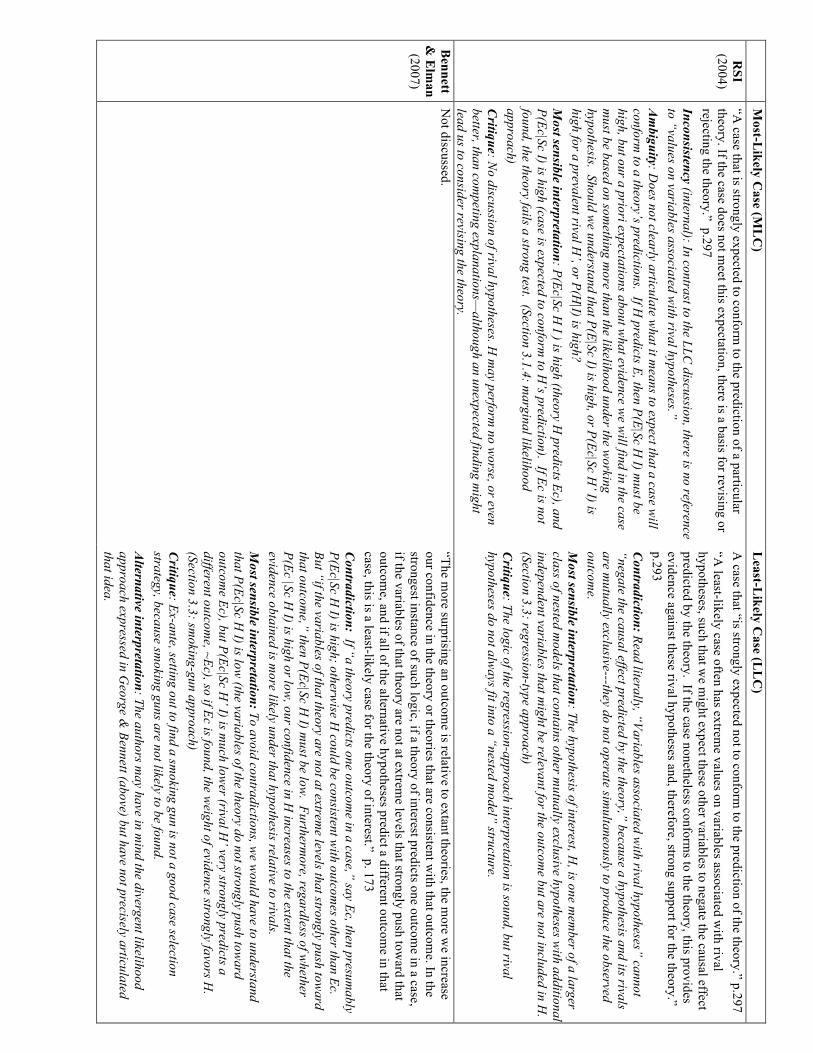
M

ost-Likely C

ase (ML

C)

Least-L

ikely Case (L

LC

) R

SI (2004)

“A case that is strongly expected to conform

to the prediction of a particular theory. If the case does not m

eet this expectation, there is a basis for revising or rejecting the theory.” p.297 Inconsistency (internal): In contrast to the LLC

discussion, there is no reference to “values on variables associated w

ith rival hypotheses.” A

mbiguity: D

oes not clearly articulate what it m

eans to expect that a case will

conform to a theory’s predictions. If H

predicts E, then P(E|Sc H I) m

ust be high, but our a priori expectations about w

hat evidence we w

ill find in the case m

ust be based on something m

ore than the likelihood under the working

hypothesis. Should we understand that P(E|Sc I) is high, or P(Ec|Sc H

’ I) is high for a prevalent rival H

’, or P(H|I) is high?

Most sensible interpretation: P(Ec|Sc H

I ) is high (theory H predicts Ec), and

P(Ec|Sc I) is high (case is expected to conform to H

’s prediction). If Ec is not found, the theory fails a strong test. (Section 3.1.4: m

arginal likelihood approach) C

ritique: No discussion of rival hypotheses. H

may perform

no worse, or even

better, than competing explanations—

although an unexpected finding might

lead us to consider revising the theory.

A case that “is strongly expected not to conform

to the prediction of the theory.” p.297 “A

least-likely case often has extreme values on variables associated w

ith rival hypotheses, such that w

e might expect these other variables to negate the causal effect

predicted by the theory. If the case nonetheless conforms to the theory, this provides

evidence against these rival hypotheses and, therefore, strong support for the theory.” p.293

C

ontradiction: Read literally, “Variables associated with rival hypotheses” cannot

“negate the causal effect predicted by the theory,” because a hypothesis and its rivals are m

utually exclusive---they do not operate simultaneously to produce the observed

outcome.

Most sensible interpretation: The hypothesis of interest, H

, is one mem

ber of a larger class of nested m

odels that contains other mutually exclusive hypotheses w

ith additional independent variables that m

ight be relevant for the outcome but are not included in H

. (Section 3.3: regression-type approach) C

ritique: The logic of the regression-approach interpretation is sound, but rival hypotheses do not alw

ays fit into a “nested model” structure.

Bennett

& E

lman

(2007)

Not discussed.

“The more surprising an outcom

e is relative to extant theories, the more w

e increase our confidence in the theory or theories that are consistent w

ith that outcome. In the

strongest instance of such logic, if a theory of interest predicts one outcome in a case,

if the variables of that theory are not at extreme levels that strongly push tow

ard that outcom

e, and if all of the alternative hypotheses predict a different outcome in that

case, this is a least-likely case for the theory of interest.” p. 173 C

ontradiction: If “a theory predicts one outcome in a case,” say Ec, then presum

ably P(Ec|Sc H

I) is high; otherwise H

could be consistent with outcom

es other than Ec. But “if the variables of that theory are not at extrem

e levels that strongly push toward

that outcome,” then P(Ec|Sc H

I) must be low

. Furthermore, regardless of w

hether P(Ec |Sc H

I) is high or low, our confidence in H

increases to the extent that the evidence obtained is m

ore likely under that hypothesis relative to rivals. M

ost sensible interpretation: To avoid contradictions, we w

ould have to understand that P(Ec|Sc H

I) is low (the variables of the theory do not strongly push tow

ard outcom

e Ec), but P(Ec|Sc H’ I) is m

uch lower (rival H

’ very strongly predicts a different outcom

e, ~Ec), so if Ec is found, the weight of evidence strongly favors H

. (Section 3.3: sm

oking-gun approach) C

ritique: Ex-ante, setting out to find a smoking gun is not a good case selection

strategy, because smoking guns are not likely to be found.

Alternative interpretation: The authors m

ay have in mind the divergent likelihood

approach expressed in George &

Bennett (above) but have not precisely articulated that idea.

!!

M

ost-Likely C

ase (ML

C)

Least-L

ikely Case (L

LC

) G

erring (2007)

“A m

ost-likely case is one that, on all [1] dimensions except the [2] dim

ension of theoretical interest, is predicted to achieve a certain outcom

e and yet does not. It is therefore disconfirm

atory.” p. 232 C

ontradiction: This definition taken literally is logically equivalent to the definition provided for a least-likely case. If w

e apply the same interpretation

of uses [1] and [2] of “dimensions” as for uses [3] and [4], respectively, then

all of the variables X2, X3... associated with the m

ore complex rival hypotheses

push toward outcom

e Ec, whereas the variable X1 associated w

ith the simpler

working hypothesis H

pushes toward ~Ec, and this case w

ould be confirmatory

for H, not disconfirm

atory. In essence, compared to the least-likely case

definition, the outcome has sim

ply been labeled ~Ec instead of Ec: the more

complex rival hypotheses that include X1 along w

ith X2, X3... predict an incorrect outcom

e (e.g. Ec), whereas H

, predicts the correct outcome (~Ec).

Most sensible interpretation: To salvage this M

LC definition, w

e would need to

interpret use [1] of “dimensions” as the independent variable(s) X1 in the

working hypothesis H

, and use [2] (rather awkw

ardly) as the dependent variable of interest (Ec vs. ~Ec). W

ith this generous interpretation, we could

then recover the likelihood approach (Section 3.1.3), where P(Ec|Sc H

I) is high, but ~Ec is observed.

“A least-likely case is one that, on all [3] dim

ensions except the [4] dimension of

theoretical interest, is predicted not to achieve a certain outcome and yet does so. It is

confirmatory.” p. 232

Most sensible interpretation: W

e understand use [4] of “dimensions” to m

ean independent variable X1 that is central to the w

orking hypothesis H, and use [3] to

mean independent variables X2, X3... associated w

ith more com

plex rival hypotheses that also include X1. If H

predicts outcome Ec, and Ec is in fact observed, then H

is (to som

e degree) strengthened relative to the rivals that predicted ~Ec due to the (countervailing) role of the additional independent variables X2, X3.... (Section 2.3: regression-type approach) C

ritique: The regression logic in our interpretation is sound, but rival hypotheses do not alw

ays fit into a “nested model” structure.

Beach &

Pedersen

(2016)

“A m

ost-likely case is one where other conditions except the X

in focus suggests that Y

should occur but it does not, implying that w

e can disconfirm X

being a cause across the population.” p. 19 C

ontradiction: This statement follow

s Gerring’s (2007) definition (above) w

ith “dim

ensions" understood (as in Gerring’s least-likely case) to be the

independent variable X1 of the working hypothesis H

. Taking Beach &

Pedersen’s statement at face value, other variables X2, X3... that are not

relevant to hypothesis H predict Y, w

hereas X1 does not, and the observed outcom

e is ~Y. But this case cannot be interpreted as most-likely for H

, and it certainly cannot disconfirm

H, since X1 assum

es values in this case that correctly predict ~Y.

“A least-likely case is w

here other conditions except X point in the direction of Y

not occurring but it does, enabling us to infer that given that it occurred w

here we least

expected it, it should also occur in more probable places. It is vital to note that the

likelihood of a causal relationship occurring in a case is based on theoretical reasons, for exam

ple, contextual conditions that are more/less conducive determ

ine the likelihood of the causal relationship occurring.” p. 19-20 M

ost sensible interpretation: see comm

ents on Gerring above.

Critique: Strong articulation of the Sinatra logic, w

hich can only be justified if we

employ a logistic regression m

odel. C

ritique: The final sentence has little sound discernable meaning. If “contextual

conditions” are theorized to affect the likelihood of X producing Y, then those conditions m

ust be explicitly included within the hypothesis that is being tested.

!!

Rohlfing (2012)

“A m

ost-likely case has a relatively high probability of confirming the proposition under scrutiny, w

hile a least-likely case goes hand in hand with a com

paratively low

probability.” p. 84 “The conditional probability of interest” for identifying a most/least-case is “P(E|H

& case), m

eaning that the probability of collecting confirming

evidence–E–is conditional on the assumption that H

is correct and in light of theory-relevant features of the chosen case.” p. 86 A

mbiguity: W

hat it means to include the “case” in the conditioning inform

ation is unclear, since the background information I (om

itted in Rohlfing’s notation) includes everything relevant w

e know about all cases. Likew

ise, the reference to “theory-relevant features” of the case is ambiguous; all details that w

e initially know about the

case should be included as background information.

Inaccuracy: P(E|H I) is the probability of finding evidence E if H

is true, not the probability of finding “confirming evidence”---the extent to w

hich evidence supports or confirm

s a hypothesis depends on likelihood ratios. Here w

e have an instance where sloppy language m

ay lead to sloppy thinking. If we call E “confirm

ing evidence,” regardless of how

large or small the likelihood is under H

, then whenever w

e observe E, we are tem

pted to think that it does indeed confirm H

, even though E may

instead weigh in favor of a rival hypothesis that predicts this evidence m

ore strongly. Interpretation: U

sing better notation, this definition asserts that a MLC

is characterized by a high value for P(Ec|Sc H I), w

hile a LLC is characterized by a low

value for P(Ec|Sc H

I). (Section 3.1.3: likelihood approach) C

ritique: This definition cannot capture the prospective notion expressed in the first quotation. If a MLC

means that P(Ec|Sc H

I) is high, then the theory makes a strong

prediction for the case, but before examining the case, that fact alone gives us no cause to believe that this case w

ill actually produce Ec; furthermore, w

hether Ec will

“confirm” H

depends on how strongly rival hypotheses predict that sam

e outcome. Sim

ilarly, knowing that P(Ec|Sc H

I) is low on its ow

n does not tell us whether w

e will

find Ec in the case. Moreover, finding Ec need not confirm

H; if P(Ec|Sc H

I) is low, there m

ay well be a rival theory that predicts Ec w

ith higher probability.

“The larger the conditional probability of the working hypothesis relative to the null hypothesis, the sm

aller the likelihood ratio is and the greater the confidence in the w

orking hypothesis following a successful test. A

least-likely case for the working hypothesis can m

eet this criterion but only if the conditional likelihood of the null hypothesis is m

uch smaller. Sim

ilarly, a most-likely case for the w

orking hypothesis offers considerable inferential leverage only when the conditional probability of the

null proposition is smaller.” p.196

Translation: Using correct term

inology and a better convention for the likelihood ratio, the above quote would instead read: “The larger the posterior probability of the

working hypothesis relative to a rival in light of the evidence, the larger the likelihood ratio, P(Ec | Sc H

I)/P(Ec | Sc H’ I), and the greater the confidence in the w

orking hypothesis follow

ing a successful test. A least-likely case for the working hypothesis, w

here P(Ec | Sc H I) is low

(following Rohlfing’s previous likelihood approach),

can meet this criterion but only if the likelihood of the case evidence conditional on the rival hypothesis is m

uch smaller than the likelihood of the evidence conditional on

the working hypothesis. Sim

ilarly, a most-likely case for the w

orking hypothesis, where P(Ec | Sc H

I) is high, offers considerable inferential leverage only when the

likelihood of the case evidence under the rival hypothesis is smaller than the likelihood of the evidence under the w

orking hypothesis.” Interpretation: C

orrectly notes that test strength depends on likelihood ratios. Associates a LLC w

ith a successful smoking gun-test: P(E|Sc H

I) is low, but P(E | Sc H

’ I) is m

uch lower for rivals, such that finding Ec supports H

. Read literally, associates a MLC

with a doubly-decisive test: P(Ec |Sc H

I) is high, but P(Ec|Sc H’ I) is m

uch low

er. Elsewhere, Rohlfing (p. 183) explicitly associates a M

LC w

ith a failed hoop test: P(Ec|Sc H I) is high, P(Ec |Sc H

’ I) is somew

hat lower, but w

e observe ~Ec. Presum

ably the intent here was to say instead that a M

LC for H

produces significant inferential leverage under the surprising outcome ~Ec for H

. C

ritique: A retrospective assessment of test strength once evidence has been found is not useful for prospective case selection.

Rapport

(2015) “ ‘Least likely’ (LL) and ‘m

ost likely’ (ML) cases, [are] also referred to as ‘hard’ and ‘easy’ cases, respectively. The form

er pose difficult tests of theories, in that—unlike M

L cases—one w

ould not expect a theory’s expectations to be borne out by a review of the case evidence.” p. 431

Most sensible interpretation: O

ne could make m

athematical sense of this statem

ent by associating “a theory’s expectations” with the predictions of the w

orking hypothesis, P(Ec | Sc H

I), and associating the earlier use of the term “expect” w

ith our ex-ante anticipation of what w

e will find, P(E|Sc I), w

hich is a weighted average

of the predictions of all plausible hypotheses under consideration. (Section 3.1.4: marginal likelihood approach).

Inaccuracy: In the formal Bayesian analysis, incorrectly identifies the m

arginal likelihood P(E|I) with the relative frequency of evidence E in a population (Appendix B).

The “Bayesian ... approach ... defines a case as LL or M

L according to a researcher’s prior confidence that the theory being tested offers a valid explanation for the outcom

e of interest in other, similar cases.” p. 433 (see also p. 450)

Interpretation: P(H|I) is low

for a LLC and high for a M

LC. (Section 3.1.2: prior probability approach)

Critique: Priors do not vary across cases.

61

Appendix C: Understanding Why Prior Probabilities Do Not Vary Across Cases

In Section 6.1.2, we argued that prior probabilities on hypotheses are determined by a given

state of background knowledge and cannot vary depending on which case we select to study.

This appendix provides some additional examples to help illustrate this point, which may seem

counterintuitive given the way language is used colloquially—while we are making decisions

about how to define or revise the scope conditions for a hypothesis, we might loosely speak

about the probability that our hypothesis explains a given case, but this meaning should not be

conflated with the Bayesian prior probability of a well-articulated, concretely-scoped hypothesis.

The overarching remedy is to carefully define the hypothesis space before making statements

about prior probabilities.

Analogies to medical testing may be one source of confusion regarding the relationship between

prior probabilities on hypotheses and specific cases.34 It is generally recognized that when

diagnosing diseases, the base rate used for the priori probability should correspond to a group

of subjects who are as similar as possible to the patient on characteristics that are known to

matter for susceptibility to the suspected illnesses. Suppose two patients display symptoms

that often accompany prostrate cancer: Martin, a 74 year-old American male, and Cheng, a

22 year-old Chinese male. In the first instance, we might use for our prior the incidence of

prostrate cancer among American men in the age group 70–75, whereas in the second instance,

we would instead use a base rate for this disease among 20–25 year-olds, ideally based on studies

of Asian men, since we know that prostrate cancer is much less common among younger men,

and also less common among Asian males (possibly due to diet). One might then think that we

have case-specific prior probabilities for the prostrate cancer hypothesis—we might be tempted

to say that Martin is a “most-likely case” for prostrate cancer, whereas Cheng is a “least-likely

case” for prostrate cancer.

The flaw in this reasoning is that the di↵erent prior probabilities in question do not correspond

to the same hypothesis. In the first instance, we are considering the hypothesis HMPC = Martin

has prostrate cancer, whereas in the second instance, we are considering a distinct hypothesis

HCPC = Cheng has prostrate cancer. These are two case-specific hypotheses. Whatever evidence

we obtain from subjecting Martin to various medical tests has no direct implications for the

34 See Appendix D for discussion of additional misconceptions arising from medical testing examples.

62

hypothesis that Cheng has prostrate cancer, and vice versa. Note also that we need to specify

the salient rival hypothesis for each problem, which would posit that the patient in question has

a di↵erent condition that produces similar symptoms (the most plausible alternative disease

a✏icting Martin may not be the most plausible alternative disease a✏icting Cheng).

A critical point to stress again in this discussion is that hypotheses and their scope conditions

must be clearly articulated before we can assign probabilities and conduct Bayesian inference.

As we emphasized in Chapter 3, a well-posed hypothesis includes a statement of any relevant

scope conditions that circumscribe the range of cases to which it applies. Once we have defined

the scope of the hypothesis, all background knowledge we have about cases that fall within

its scope contributes to the prior probability of that hypothesis—regardless of whether the

information we know about a given case seems to support or to undermine the hypothesis

relative to the rival(s) under consideration.

As an example, suppose we are considering a hypothesis from the literature that is understood to

apply to all developing countries—to be concrete, takeHSE = Stolen elections are the key causal

factor that motivates democratic mobilization in developing countries, [via mechanism M ]. Now

suppose we have salient background knowledge about two developing countries—Serbia and the

Philippines. Let’s say our background information about the Serbian case moderately supports

HSE over the rival hypothesisHCE = Autonomous communal elites are the key causal factor that

motivates democratic mobilization in developing countries, but our background knowledge of

the Philippines (from reading Slater (2009)) strongly supports HCE over HSE .35 Our prior odds

on HSE vs. HCE then weakly favor the communal-elites hypothesis. These are our prior odds

regardless of which developing country we choose to study next—whether China, the Ukraine,

Venezuela, or Burma. If our study will involve additional research on the Serbian and/or

Philippine case(s), our prior odds still weakly favor HCE over HSE . These prior odds remain

unchanged regardless of whether we plan to gather new evidence for the Serbian case first, or

for the Philippine case first. Even though we have di↵erent background information for each

individual case, the priors on HSE vs. HCE reflect our combined background information about

both cases. Because neither of these hypotheses is case-specific, we cannot have case-specific

priors, and it would not make sense to assert that we have a di↵erent degree of confidence that

HSE provides a better explanation than HCE for the Serbian case compared to the Philippine

35 See Chapter 4.

63

case.

Now we might instead decide that in light of our background information, it is worth modifying

the scope conditions on the stolen-elections hypothesis. One approach would be to limit its

scope to Eastern Europe and then conduct additional research on Eastern European cases to

see whether the evidence further supports this narrower stolen-elections hypothesis over rivals.

Our new hypothesis, HEESE , does not apply to the Philippines, so any background information

we have about that case is irrelevant to the prior odds on HEESE vs. a rival that includes Eastern

Europe within its scope. So here it makes no sense to ask about the probability that HEESE

explains the Philippines, because this case lies outside its scope. And again our prior odds

remain fixed regardless of which Eastern European case we study next.

Alternatively, we might pose a new hypothesis that applies to both Eastern European and

Asian cases: HS/C = Stolen elections are the key factor that motivates democratic mobilization

in Eastern Europe, whereas autonomous communal elites are the key factor that motivates

democratic mobilization in Asia, and compare it to the original hypothesis HSE , which holds

that the stolen-elections logic applies in both regions. Now our Serbian background information

(IS) favors neither HS/C nor HSE , while our Philippine background information (IP ) stronglysupports H over HSE . Our prior odds, based on IS IP , then strongly supports HS/C over HSE .

Again, these prior odds are determined by our unique state of knowledge IS IP , which remains

unchanged regardless of which county in Eastern Europe or Asia we contemplate studying.

64

Appendix D: Understanding Marginal Likelihoods in the Context of Case-Based Research

Another misconception regarding the application of probabilistic reasoning to case selection in

qualitative research concerns the interpretation of the marginal likelihood in Bayes’ rule—it is

sometimes incorrectly taken to be the relative frequency of some evidence E in a population

of cases. This misconception, which is evident in Rapport’s (2015) analysis, may be fairly

widespread and thus merits some careful attention.

Referring to Bayes’ rule in the following form (where we have explicitly including the background

information, which the author omits):

P (H |E I) = P (H | I)P (E |H I)P (E | I) , (D1)

Rapport (2015:448) writes that: “Bayesian inference rests on three legs: the strength of one’s

prior beliefs about a theory, how closely evidence in a case fits theoretical expectations, and the

typicality of the evidence in a case.” We have argued that Bayesian inference in fact depends on

how much better or worse the evidence fits the respective expectations of competing theories, as

becomes more evident when working with the odd-ratio version of Bayes’ rule. But the greater

concern at hand is whether “typicality of the evidence in a case” is gauged by comparison across

cases, or by comparison across theories.

Rapport (2015:448) defines P (E | I) in Bayes’ rule as “the overall probability of observing E

at all given its prevalence in the population of interest—the broader class from which the case

is drawn.” Rapport (2015:449) accordingly asserts that: “one’s confidence in the theory ...

increases if the evidence one observes rarely occurs in comparable cases,” thinking this should

make the denominator P (E | I) in Bayes’ rule small and hence boost posterior probability.

However, P (E | I) has nothing to do with the prevalence of evidence E in other cases. This

marginal probability should instead reflect our surprise at seeing the evidence E in the case

at hand, based on our prior confidence in rival theoretical explanations that might account for

the evidence—not on some sort of relative frequency of how often similar evidence arises across

cases. Later in his discussion of Bayes’ rule, Rapport (2015:448) correctly writes that “P (E)

captures all the ways the evidence might have been generated in addition to the mechanisms

specified by the theory of interest.” But throughout, he conflates these two very di↵erent

notions: a weighted average across di↵erent cases, and a weighted average across di↵erent

65

theories.36

The confusion regarding P (E | I) may be dispelled by (1) using notation that explicitly cap-

tures the potentially case-specific nature of the evidence, and (2) remembering that Bayesian

probabilities are often unrelated to relative frequencies, as elaborated below.

1. Handling Case-Specific Evidence

In qualitative research, we work with detailed evidence that is often specific to a particular

case. To help keep this reality in mind, we will denote evidence gathered from case Ck as ECk .

With this more explicit notation, Bayes’ rule becomes:

P (HA |ECkI) = P (HA | I) P (ECk |HA I)P (ECk | I)

(D2)

Our background information may also contain case-specific knowledge, which we can highlight

by writing I = (I1 · · · Ik · · · ) I0, where a term Ik represents facts specific to case Ck, and I0contains common background knowledge, which at minimum specifies the mutually exclusive

and exhaustive hypotheses {HA, HB, ...} under consideration. Using the law of total probability,

we can decompose the marginal likelihood P (ECk | I) as follows:

P (ECk | I) = P (HA | I)P (ECk |HA I1 · · · Ik · · · I0)+ P (HB | I)P (ECk |HB I1 · · · Ik · · · I0) + · · · .

(D3)

This notation should clarify that the marginal likelihood has little to do with the prevalence of

similar-looking evidence that might be found in other cases. It is the likelihood of occurrence

of the particular evidence ECk in the particular case Ck, given the relevant background infor-

mation Ik I0, averaged over the possible hypotheses that might underpin the case dynamics,

weighted by our prior confidence in these rival explanations.37 If we include enough detail

36 This misconception may also underlie Rapport’s (2015:435) earlier claim that the Bayesian “approach attendsmore to the population from which a case was drawn and defines a case as LL [least likely] or ML [most likely]according to a researcher’s prior confidence that the theory being tested o↵ers a valid explanation for theoutcome of interest in other, similar cases.” Compared to more conventional attitudes to qualitative researchthat tend to be grounded in extrapolations of frequentist reasoning, Bayesian conceptualizations are far less,not more, tied to “populations from which a case was drawn,” and allow the researcher to assess within-caseevidence on its own terms rather than exclusively in comparison to “other, similar cases.”

37 It is possible for outside evidence to a↵ect the likelihoods and marginal likelihoods in the case under inves-tigation, but only indirectly. These probabilities are conditional on I1I2 · · · , which might include evidencepreviously collected in other cases. In turn, this previous evidence might have been used for instance to tune

66

(regarding specific events in the country, direct quotations from a particular politician), we can

always ensure that the “evidence one observes rarely occurs in comparable cases,” (Rapport

2015:449)—for instance, it would hardly make sense to ask whether we might observe Cardinal

Sin of the Philippines calling the people into the streets to protect retreating coup leaders fol-

lowing Marcos’ fraudulent election when conducting a case study of democratic mobilization in

Vietnam or Burma. Yet the uniqueness of the evidence to the case is not what increases our

confidence in a theory; it is the uniqueness of the evidence to a theory that boosts the posterior

probability.

In sum, for qualitative social science, marginal likelihoods in Bayes’ theorem generally do not

reflect “prevalence in the population” of cases (Rapport 2015:449), because we typically observe

a unique piece or body of evidence in the context of a particular case. Even if we were to coarse-

grain the evidence into broad “clue types” for the sake of greater comparability across cases,

the marginal probability of evidence ECk cannot be equated with the relative frequency of its

clue type in some population of interest. Outside of survey research, cases or case evidence can

rarely be viewed as random samples drawn from some delineated and exchangeable population.

2. Bayesian Probabilities vs. Relative Frequencies

Introductions to Bayes’ theorem routinely include what we might call a “dreaded diagnosis”

example from medical testing, similar to our worked example at the end of Chapter 2. Such cal-

culations nicely highlight the importance of taking prior information into account, but they may

also lead to some confusion between Bayesian probabilities and frequencies that can contributes

to misinterpretations of the marginal likelihood in the context of case selection.

Reprising our Chapter 2 example, suppose Patient X tests positive (+) for disease D according

to some standard diagnostic test ⌧ . How worried should X be? The answer will depend

on information about the reliability of the diagnostic test, and prior expectations about the

prevalence of the disease. Assume we know nothing else about the particulars of X’s medical

model parameters, which then can a↵ect the likelihoods generated by the theories regarding new evidence ob-served in the current case Ck. But this indirect influence acts primarily through the hypotheses, and does notseem to be what Rapport had in mind. Note also that if we alter the set of hypotheses under consideration, weare changing the common background information I0, and P (ECk | I) will accordingly change as well. Hence,contrary to Rapport’s (2015:449) assertion, the numerical value of the denominator P (ECk | I) definitely neednot remain “constant” as the researcher “goes back and forth between theory and evidence in di↵erent cases.”

67

condition or history other than the results of the test, but we do have information I about the

past performance of the test on a large number of other patients, and about the prevalence of

the disease in the general population. The probability of interest is then:

P (D | ⌧+ I) = P (D | I)P (⌧+ |D I)P (⌧+ | I) =

P (D | I)P (⌧+ |D I)P (D | I)P (⌧+ |D I) + P (D | I)P (⌧+ |D I) . (D4)

The hypotheses in question concern whether patient X su↵ers from the disease (D) or not

(D), and the evidence consists of a positive result on a diagnostic test ⌧+. The point of the

example is to emphasize that even if the true positive rate P (⌧+ |D I) is moderately high (but

definitely less than perfect), and the false positive rate P (⌧+ |D I) is moderately (but not

extremely) small, then the posterior probability of having the disease can still be much smaller

than the true positive rate of the test, if overall the disease is extremely rare in the sense that

P (D | I) ⌧ P (D | I) = 1� P (D | I).

A common misunderstanding that seems to be taken from this type of example is that prior

probabilities can be identified with base rates, and marginal likelihoods can be identified with

relative frequencies in a population. These assumptions are unproblematic in the above ex-

ample, but they are not justifiable more generally. In the medical testing example, the prior

P (D | I) could be estimated as the fraction of individuals from the population (or more practi-

cally, from a random sample drawn from the population) that do su↵er from the disease, and

the marginal likelihood P (⌧+ | I) could be estimated as the overall fraction of individuals who

(would) test positive because we are e↵ectively treating all individual cases as exchangeable

samples drawn at random from the larger population. However, if we include more specific in-

formation about the condition of patient X into our background information, replacing I with

more detailed IX , then P (D | IX) can no longer be interpreted as the base rate of the disease

in the overall population; it instead represents our prior belief that X has the disease given

this patient-specific medical information, and P (⌧+ | IX) is the probability that the particular

patient X will test positive whether su↵ering from the disease or not. In the idealized limiting

case where IX contains exceptionally detailed physiological information about X and biological

information about both the test and the disease, then P (⌧+ | IX) would have essentially nothing

to do with any population of other patients, but should instead reflect our knowledge of how the

individual physiology of X and the biochemical operation of the test might e↵ect the outcome

of the test in this one case.

In the original formulation of the medical example,

68

(i) the propositions of interest concern whether a particular patient X has a disease D or

not;

(ii) the population of all possible patients is considered exchangeable, meaning in this context

that we know nothing about X other than the test result, and X is assumed to have the

same propensities as any other patient; and

(iii) the possible evidentiary outcomes (i.e, the test results ⌧+ or ⌧�) are course-grained and

could be measured for any individual patient.

In this context, the marginal probability P (⌧+ | I) can be consistently estimated as a rela-

tive frequency across cases in the population. But in qualitative case research, where we are

interested in the marginal probability P (ECk | I),

(i0) the propositions of interest are often general explanatory theories which we hope apply

to all cases satisfying the stated scope conditions;

(ii0) cases are known or expected to have unique features, and hence are not exchangeable;

and

(iii0) the possible evidentiary outcomes tend to be fine-grained, are not easily denumerable,

and generally vary from case to case.

Therefore, in the latter context, P (ECk | I) cannot be interpreted or estimated as a rate of

prevalence in some population of cases.