A Bayesian hierarchical mixture model with continuous-time ...

Bowdoin College Bowdoin College

Bowdoin Digital Commons Bowdoin Digital Commons

Honors Projects Student Scholarship and Creative Work

2021

A Bayesian hierarchical mixture model with continuous-time A Bayesian hierarchical mixture model with continuous-time

Markov chains to capture bumblebee foraging behavior Markov chains to capture bumblebee foraging behavior

Max Thrush Hukill Bowdoin College

Follow this and additional works at: https://digitalcommons.bowdoin.edu/honorsprojects

Part of the Apiculture Commons, Bioinformatics Commons, Biostatistics Commons, Data Science

Commons, Entomology Commons, Statistical Methodology Commons, and the Statistical Models

Commons

Recommended Citation Recommended Citation Hukill, Max Thrush, "A Bayesian hierarchical mixture model with continuous-time Markov chains to capture bumblebee foraging behavior" (2021). Honors Projects. 300. https://digitalcommons.bowdoin.edu/honorsprojects/300

This Open Access Thesis is brought to you for free and open access by the Student Scholarship and Creative Work at Bowdoin Digital Commons. It has been accepted for inclusion in Honors Projects by an authorized administrator of Bowdoin Digital Commons. For more information, please contact [email protected].

A Bayesian hierarchical mixture model withcontinuous-time Markov chains to capture

bumblebee foraging behavior

An Honors Paper for the Department of MathematicsBy Max Thrush Hukill

Bowdoin College, 2021© 2021 Max Thrush Hukill

Abstract

Some say that unto bees a share isgiven of divine intelligence...

–Virgil, Georgics IV: 221–222

The standard statistical methodology for analyzing complex case-control studies inethology is often limited by approaches that force researchers to model distinct aspects ofbiological processes in a piecemeal, disjointed fashion. By developing a hierarchical Bayesianmodel, this work demonstrates that statistical inference in this context can be done using asingle coherent framework. To do this, we construct a continuous-time Markov chain (CTMC)to model bumblebee foraging behavior. To connect the experimental design with the CTMC,we employ a mixture model controlled by a logistic regression on the two-factor design matrix.We then show how to infer these model parameters from experimental data using Markovchain Monte Carlo and interpret the results from a motivating experiment.

1

Acknowledgements

Despite the tragedy of the past fifteen months, the following people have risen to the occasionand made this experience a profoundly fulfilling capstone project for my undergraduateeducation. I am honored to have had the priviledge to work with all of them.

This project would not have been possible were it not for the efforts of Professor PattyJones and her lab. They supplied the data and initial statistical analyses, in addition to thebiological motivation for my model. For all of this, I am deeply grateful.

I want to thank the Bowdoin Mathematics Department for offering me a wonderful placeto grow intellectually these past four years. Not only have they supported me throughoutthis project in hosting and encouraging my two honors talks, but they’ve instilled in me apassion for mathematical learning that will persist for years to come. I particularly want tothank Professor William Barker, Professor Naomi Tanabe, and Sam Harder for bringing meinto the major in the first place, and for solidifying my deep love of mathematical problemsolving. I am so fortunate to have met them when I did.

I want to thank my classmates over the years who have made the major the experience thatit has been. The collaboration, care, and sense of humor that have defined my time herewill remain in my fondest memories. Along those lines, I am particularly indebted to JayaBlanchard, Dan Ralston, John Hood, Junyoung Hwang, Josh George, Charlotte Hall, BryanVargas, Huma Dadachanji, Juliana Taube, Sam Harder, and Connor Fitch.

I want to thank my advisor, Professor Jack O’Brien, for his integral role in my intellectualand statistical development. Ever since I entered his office as a curious calculus student, hehas encouraged my study of probability and statistics with remarkable conviction. From hisgenuinely inspirational lectures, to his reliable assistance in office hours, to his bravery indebugging code, to his empathetic and deeply interested support as a research advisor, Jackhas demonstrated the best of what the small liberal arts college experience has to offer. Icould not be more grateful to him.

I want to thank my parents, Jane Thrush and Warren Hukill, and my partner, MiraiHutheesing, for their steadfast support and willingness to endure ceaseless presentationpractice. I simply could not have done this without you three.

Finally, I want to thank the brave bumblebees who gave their humble lives to make thisscience possible. Humanity owes you all.

2

Preface

In their little bodies beats a mightyspirit.

–Virgil, Georgics IV: 83

The following thesis presents a novel implementation of continuous-time Markov chainsfor statistical analysis. I begin with the mathematical foundations for the work, taking anabridged tour through probability theory, Markov processes, and Markov chain Monte Carloinference methodology. I then present the motivating biological experiment, going throughthe intricacies of the set-up and standard approach to statistical analysis. After reflecting onthe limitations of those current methods, I present the novel Bayesian hierarchical mixturemodel that defines the core of my work. After fully specifying the model, I offer an outline ofmy inference strategy, relying principally on Markov chain Monte Carlo, coded entirely inbase R. With the tools defined, I then present simulation studies to test the theoretical limitsof the algorithm. I proceed then to applying the inference algorithm to real data collected bythe lab of Dr. Patty Jones at Bowdoin College. I apply various model checking methods tointerrogate the veracity of the parametric inference accomplished by my model. I concludewith next steps, both immediate and more sophisticated, for augmenting this solution to animportant statistical problem.

Please note that I fully built, tested, and applied two distinct algorithms: one usingcontinuous-time Markov chains, and one using discrete-time Markov chains as an approxima-tion. The latter has been moved to the appendix for clarity. The second appendix containschapter-specific hints, such as proofs, supplementary figures, and interesting details. Feelfree to jump between the main body of the work and these appendices. I, for one, foundit immensely helpful to keep the discrete-time approximation in mind when developing thecontinuous-time model. Thank you for your readership!

The code for both models and all figures will be supplied in an open-source manner onGitHub. In the coming summer of 2021, we will be translating this work into a manuscriptfor journal submission, at which point the code will become available. For those members ofposterity interested in this information, please reach out to me at [email protected].

3

Contents

1 Mathematical Background 6

1.1 Probability and statistical theory . . . . . . . . . . . . . . . . . . . . . . . . 6

1.1.1 Fundamentals . . . . . . . . . . . . . . . . . . . . . . . . . . . . . . . 6

1.1.2 Likelihoods . . . . . . . . . . . . . . . . . . . . . . . . . . . . . . . . 7

1.2 Markov chains . . . . . . . . . . . . . . . . . . . . . . . . . . . . . . . . . . . 8

1.2.1 Discrete-time Markov chains . . . . . . . . . . . . . . . . . . . . . . . 8

1.2.2 Continuous-time Markov chains . . . . . . . . . . . . . . . . . . . . . 8

1.3 Markov chain Monte Carlo . . . . . . . . . . . . . . . . . . . . . . . . . . . . 10

2 Experimental Design 14

2.1 Experimental motivation . . . . . . . . . . . . . . . . . . . . . . . . . . . . . 14

2.1.1 Physical description and core questions . . . . . . . . . . . . . . . . . 14

2.1.2 Translation of video data into coordinates . . . . . . . . . . . . . . . 15

2.2 Standard approach to statistical analysis . . . . . . . . . . . . . . . . . . . . 16

2.2.1 Generalized linear-mixed models . . . . . . . . . . . . . . . . . . . . . 16

2.2.2 Limitations of the standard method . . . . . . . . . . . . . . . . . . . 18

3 Statistical Model 20

3.1 The Journey Model . . . . . . . . . . . . . . . . . . . . . . . . . . . . . . . . 20

3.1.1 Hierarchical model . . . . . . . . . . . . . . . . . . . . . . . . . . . . 22

3.1.2 Foraging journey as a continuous-time Markov chain . . . . . . . . . 23

3.1.3 Regression effects . . . . . . . . . . . . . . . . . . . . . . . . . . . . . 23

3.1.4 Training data: the missing link . . . . . . . . . . . . . . . . . . . . . 24

3.2 Continuous-time model . . . . . . . . . . . . . . . . . . . . . . . . . . . . . . 25

3.2.1 CTMC likelihood . . . . . . . . . . . . . . . . . . . . . . . . . . . . . 26

4 Inference 28

4.1 Transforming the state space . . . . . . . . . . . . . . . . . . . . . . . . . . . 28

4

4.2 Continuous-Time Markov chain inference . . . . . . . . . . . . . . . . . . . . 28

4.2.1 Move 1: Metropolis-Hastings sampling of regression coefficients . . . 29

4.2.2 Move 2: Metropolis-Hastings sampling of rate matrix parameters . . 30

4.2.3 Move 3: Training state posterior calculation . . . . . . . . . . . . . . 30

4.2.4 Compound CTM Algorithm . . . . . . . . . . . . . . . . . . . . . . . 31

4.3 Convergence . . . . . . . . . . . . . . . . . . . . . . . . . . . . . . . . . . . . 32

5 Simulation Studies 34

6 Data Analysis 40

6.1 Regression and training results . . . . . . . . . . . . . . . . . . . . . . . . . . 40

6.2 Model checking . . . . . . . . . . . . . . . . . . . . . . . . . . . . . . . . . . 43

6.3 Dwell-times revisited . . . . . . . . . . . . . . . . . . . . . . . . . . . . . . . 45

7 Future Directions 47

Appendices 49

A Discrete-Time Model 50

A.1 Discrete-Time Model . . . . . . . . . . . . . . . . . . . . . . . . . . . . . . . 50

A.1.1 Link between journey data and training state . . . . . . . . . . . . . 50

A.1.2 Link between training state and experimental design . . . . . . . . . 52

A.1.3 Hierarchical model . . . . . . . . . . . . . . . . . . . . . . . . . . . . 52

A.2 Discrete-Time Algorithm . . . . . . . . . . . . . . . . . . . . . . . . . . . . . 53

A.2.1 Move 1: Gibbs sampler for updating the transition matrices . . . . . 53

A.2.2 Move 2: Metropolis-Hastings sampling of the regression coefficients . 54

A.2.3 Move 3: Training state posterior calculation in the DTM . . . . . . . 54

A.2.4 Compound DTM Algorithm . . . . . . . . . . . . . . . . . . . . . . . 55

A.3 Simulation Studies . . . . . . . . . . . . . . . . . . . . . . . . . . . . . . . . 56

A.4 Real Data . . . . . . . . . . . . . . . . . . . . . . . . . . . . . . . . . . . . . 59

A.5 Model Checking . . . . . . . . . . . . . . . . . . . . . . . . . . . . . . . . . . 64

B Chapter-Specific Appendices 65

5

Chapter 1

Mathematical Background

1.1 Probability and statistical theory

1.1.1 Fundamentals

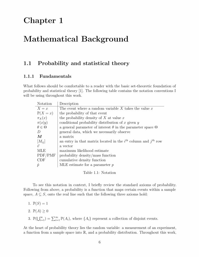
What follows should be comfortable to a reader with the basic set-theoretic foundation ofprobability and statistical theory [1]. The following table contains the notation conventions Iwill be using throughout this work.

Notation DescriptionX = x The event where a random variable X takes the value xP(X = x) the probability of that eventπX(x) the probability density of X at value xπ(x|y) conditional probability distribution of x given yθ ∈ Θ a general parameter of interest θ in the parameter space ΘD general data, which we necessarily observeM a matrix[Mij] an entry in that matrix located in the ith column and jth row~v a vectorMLE maximum likelihood estimatePDF/PMF probability density/mass functionCDF cumulative density functionp̂ MLE estimate for a parameter p

Table 1.1: Notation

To see this notation in context, I briefly review the standard axioms of probability.Following from above, a probability is a function that maps certain events within a samplespace, A ⊆ S, onto the real line such that the following three axioms hold:

1. P(S) = 1

2. P(A) ≥ 0

3. P(⋃∞i=1) =

∑∞i=1 P(Ai), where {Ai} represent a collection of disjoint events.

At the heart of probability theory lies the random variable: a measurement of an experiment,a function from a sample space into R, and a probability distribution. Throughout this work,

6

I will refer to individual event probabilities with P and probability distributions with π. Forexample, if I flip a fair coin with outcomes X ∈ {H,T}, the probability of landing on heads isP(H) = 0.5. However, the probability mass of my Bernoulli random variable X at the pointrepresenting heads would be written as π(X = H) = 0.5. These reflect the same process, butwith different emphases.

1.1.2 Likelihoods

At the heart of classical (or frequentist) statistics lies the concept of the likelihood, a functionthat encodes the probability of the data given the model parameters. For example, supposewe had a series of data independently and identically distributed (iid) from the same Poissonrandom variable. We would write this

x1, x2, . . . , xNiid∼ Poisson(λ).

We would then write the likelihood as

L(D|Θ) = π(X1 = x1, X2 = x2, . . . Xn = xn) =N∏i=1

π(Xi = xi|λ) =N∏i=1

e−λλxi

xi!.

Notice, it is composed of a product of probability density/mass functions, following fromthe assumption of independence. As we’ll soon see, these likelihood structures can becomearbitrarily complex to cope with real data.

Much of classical statistics focuses on deriving maximum likelihood estimates (MLEs)for Θ. In an MLE, the log of the likelihood is maximized, yielding the parameter values that(unsurprisingly) maximize the value of the likelihood. The MLE provides the fit of Θ with D,without including any other information that the researcher may have about Θ.

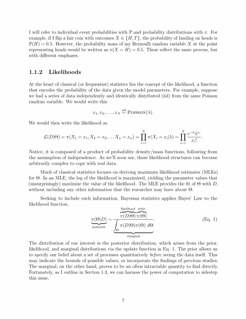
Seeking to include such information, Bayesian statistics applies Bayes’ Law to thelikelihood function,

π(Θ|D)︸ ︷︷ ︸posterior

=

likelihood︷ ︸︸ ︷π(D|Θ)

prior︷ ︸︸ ︷π(Θ)∫

Θ

π(D|Θ)π(Θ) dΘ︸ ︷︷ ︸marginal

. (Eq. 1)

The distribution of our interest is the posterior distribution, which arises from the prior,likelihood, and marginal distributions via the update function in Eq. 1. The prior allows usto specify our belief about a set of processes quantitatively before seeing the data itself. Thismay indicate the bounds of possible values, or incorporate the findings of previous studies.The marginal, on the other hand, proves to be an often intractable quantity to find directly.Fortunately, as I outline in Section 1.3, we can harness the power of computation to sidestepthis issue.

7

1.2 Markov chains

Markov chains are a foundational stochastic process ubiquitous in scientific modeling. Theconcept of Markov chains forms a consistent through line for this thesis in two key ways:how I model the data, and how I infer the model parameters. Specifically, the data aremodelled by a novel continuous-time Markov chain, while the guiding inference strategy relieson Markov chain Monte Carlo—a method for simulating a Markov chain to approximate adistribution of interest. The stochastic process introduction has been adapted from [2], [3],and [4].

1.2.1 Discrete-time Markov chains

A stochastic process in discrete time s ∈ N is a sequence of random variables Xs indexed bytime, represented X = {Xs : s ∈ N}. The range of Xs is called the state space S, with eachXs taking a state within S. In discrete time, the Markov property states that

P(Xt = j|X0 = i0, X1 = i1, . . . , Xt−2 = it−2, Xt−1 = i) = P(Xt = j|Xt−1 = i)

= Pij,

where indices {i0, . . . , it−2, i, j} ∈ N, and states {Xi} ∈ S for all indices. In other words, thesystem’s future behavior does not depend on its past behavior, given its present state. (Astochastic process that has the Markov property is said to be a Markov chain.) Note thatthe notation Pij reflects the probability of transitioning from state i to state j in one timestep. We can then define the transition matrix specific to a given Markov chain:

P = [Pij],

with the necessary condition that∑

j∈S Pij = 1. This condition ensures that we’ve formed aprobability mass function for the process of going from state i to the next state j; that is, alloptions of j are not only enumerated, but they’re assigned probabilities that will sum to 1.Consequently, transition matrices are square of size |S| × |S|.

1.2.2 Continuous-time Markov chains

To extend the ideas of a DTMC to continuous time, we’ll consider cases of discretely valuedspaces, but now with time on the positive real line, as we experience it in the natural world.The Markov Property can be defined in these contexts as well: in a continuous stochasticprocess, denoted {X(t)|t ≥ 0} with some arbitrary state space S, the Markov property isdefined as

P(X(t) = j|X(s) = i,X(tn−1) = in−1, . . . , X(t1) = i1) = P(X(t) = j|X(s) = i)

where 0 ≤ t1 ≤ t2 ≤ · · · ≤ tn−1 ≤ s ≤ t is any non-decreasing sequence of n + 1 times(ignoring zero), and i1, i2, . . . , in−1, i, j ∈ S are any n+ 1 states [3].

8

There are two critical features of this definition. First, these processes forget their past,as the conditional probability that depends on the entire chain’s past is indistinguishablefrom that which is only conditioned on the previous state. I refer to this as memorylessness.Second, at least here, these processes are time-homogeneous: for any s ≤ t and any statesi, j ∈ S, we find that

P(X(t) = j|X(s) = i) = P(X(t− s) = k|X(0) = i).

The time spent in any given state i, denoted ti, is a random variable called the dwell-time .In the appendix corresponding to this chapter, I show that these dwell-times are necessarilyexponentially distributed. Recall the definition of the exponential random variable with meanλ−1,

π(x|λ) = λe−λx.

Using the exponential nature of dwell-times, we can consider an equivalent constructionof a CTMC that will make certain things easier to work with. Consider the following processusing |S| alarm clocks.

1. We begin in some state i of the chain at time t = 0.

2. At t = 0, we set |S| alarm clocks, one for each possible state j ∈ S (with j 6= i) thatthe chain could transition to. These alarm clocks are exponential random variableswith rates, λi,j.

3. When the first alarm clock detonates, we transition to that state. This is now state j.

4. We reset the alarm clocks and continue.

This process is clearly a Markov chain in continuous time, but with dwell-times arising fromminima of various exponentials. We can cluster these exponential rate parameters into arate matrix Q. Note, this is of the same square form as the DTMC transition matrices,although instead of representing probabilities, it represents infinitesimal rates. However, thediagonal entries are still undefined: in the CTMC construction it no longer makes sense totransition back to the current state; the dwell-time construction already accounts for that.In the DTMC, we’d “transition” each time unit regardless of whether or not we’d actuallymoved; in the CTMC, we dwell for a certain amount of time until we transition to a newstate. As such, the diagonal entries of Q must be equal to the negative of the sum of thecorresponding row:

−Qi,i ≡∑i,j 6=i

Qi,j.

The rate matrix (also called the infinitesimal or generator matrix), in conjunction witha state space and starting distribution, are sufficient to uniquely define a CTMC [3]. Thisthen is the critical object of study in much the same way that a transition matrix functionsfor DTMCs. We will use this rate matrix to develop a CTMC likelihood (see Chapter 3).

9

To better understand these infinitesimal rate matrices, we will consider the instantaneoustransition matrix at a given time, P (t). We’ll need to employ the Chapman-Kolmogorovequations in continuous time [3]. The change in the transition probabilities can be given as apair of matrix differential equations, stated

P ′i,j =∑k∈S

Pi,k(t)Qk,j or in matrix form P ′(t) = P (t)Q (Forward)

P ′i,j =∑k∈S

Qi,kPk,j(t) or in matrix form P ′(t) = QP (t) (Backward)

These are simple first order differential equations in matrix form, and so often tractable.Just as the solution to the initial value problem f ′(t) = cf(t) with f(0) = f0 is f(t) = f(0)ect,the solution to these equations will be the matrix exponential.

P (t) = eQt ≡∞∑n=0

Qntn

n!,

where P (0) = I. This is the unique solution to the Chapman-Kolmogorov equations, anddemonstrates the theoretical (if not practical) power the rate matrix has, in that it directlydetermines each instantaneous transition matrix for the CTMC [3]. (Proofs in cited sources.)

1.3 Markov chain Monte Carlo

Markov chain Monte Carlo (MCMC) is a powerful tool used across disciplines of modernscience to recover complex probability distributions that cannot be analyzed exactly. Thesheer quantity and diversity of applications of MCMC have earned it a place among themost important advances in empiricism to date, with one of its key examples, the Metropolis-Metropolis-Hastings algorithm (MHA), often cited as among the top-ten most importantalgorithms of the 20th Century [5], [6], [7]. It has been a paradigm-shifting development fornot just statistics, but the use of probabilistic models across the sciences.

The details supporting MCMC have been left as citations. I will sketch the contours ofthe theory leading up to it (particularly the proof of the MHA, located in the appendix) inorder to buttress intuition for this revolutionary idea.1

To begin, recall the definition of the posterior from Bayes’ Law:

π(Θ|D)︸ ︷︷ ︸posterior

=π(D|Θ)π(Θ)∫

Θπ(D|Θ)π(Θ) dΘ

.

Our interest lies in the posterior distribution, and how to draw samples from it. Suppose wehave no way to solve the integral analytically. Fortunately, MCMC allows sampling from the

1Please note, the following abridged tour of the theory behind MCMC contains elements that have beenadapted from the very elegant synopsis composed by my friend and classmate, Huma Dadachanji (Bowdoin2020), for our Bayesian statistics course in December 2019. See [2] for more complete details.

10

posterior distribution. Then, with these samples, we can construct an approximation of theposterior distribution.

A Markov chain is said to be ergodic when it meets the following three criteria:

• Irreducible: each state of the Markov chain can communicate with all other states(meaning for all states i there exists some path to state j in finite steps).

• Aperiodic: the chain contains no closed loops that induce periodic cycles.

• Recurrent: the chain has a positive probability of returning to each state.

The power behind ergodicity lies in the Fundamental Limit Theorem for Ergodic MarkovChains, which states that the limiting distribution of an ergodic Markov chain is the uniquestationary distribution (proof in Debrow, Chapter 3.10). The following paragraph furtherdevelops these definitions.

Consider a stochastic transition matrix P with state space S, where the states representvalues for our parameters of interest, θ ∈ Θ. Indeed, this means that our state space hasbecome infinite, and P is thus referred to as a kernel. We can now define the stationarydistribution, which is a row vector ~λθ = {λθ : θ ∈ Θ} over the state space such that λP = λ fora given Markov chain. Notice, the action of the Markov chain does not alter this distribution.Next, let us define a limiting distribution of a Markov chain, which is a row vector such that

λi = limN→∞

1

N

N∑m=1

Pmij ,

for all initial states i. This means that the distribution of λ is independent of the startingstate. As it turns out, limiting distributions are necessarily stationary distributions. But thenthe question arises, is my given stationary distribution the one and only limiting distribution?Hence the power of ergodicity (see above).

The last piece we need is reversibility, a condition met by Markov chains that satisfy

πjPji = πiPij,

for all i, j ∈ S, where π is a stationary distribution. It can be shown that if a reversible chainis also ergodic, then π must be the one and only stationary distribution of P (proof in [2],Chapter 5). This condition is known as detailed balance.

The goal of MCMC then rests in constructing a P whose limiting (and thus stationary)distribution is a specific posterior distribution, π(θ|D). We now know this can be accomplishedby ensuring that the chain is reversible and ergodic. This can be achieved using the Metropolis-Hastings Algorithm (MHA).

The Metropolis-Metropolis-Hastings Algorithm. We seek to sample from atarget distribution, π∗, but cannot do so directly. However, we are able to sample from astochastic matrix Q that can propose a new state j given a current state i (using S as thestate space for both of these matrices). We can then construct the following Markov chain:

11

• Initialize the chain X0 to some state i ∼ α, where α is a distribution over S. Set t = 1.

• For t > 0:

– Propose (sample) j from Qij.

– Then, calculate

αij =π∗(j) ·Qji

π∗(i) ·Qij

.

– Sample U ∼ UNIFORM(0, 1).

– If U < αij,

∗ Xt+1 ← j

– Else

∗ Xt+1 ← Xt

– Set t = t+ 1.

If Q is ergodic, the MHA constructs a Markov chain X with a stationary distribution ofπ∗ (proven in appendix). Despite its apparent brevity, this algorithm possesses a staggeringquantity of potential.

Consider the specific case where π∗ is our posterior of interest π(Θ|D). Notice thebeauty of the Metropolis-Hastings ratio when we incorporate that fact:

αij =Qji

Qij

· π∗(j)

π∗(i)

=Qji

Qij

· π(D|Θj)π(Θj)∫Θπ(D|Θ)π(Θ) dΘ

÷ π(D|Θi)π(Θi)∫Θπ(D|Θ)π(Θ) dΘ

=Qji

Qij

· π(D|Θj)π(Θj)

π(D|Θi)π(Θi).

Sometimes the universe is kind to us—the intractable integrals of the marginal cancel, meaningwe only need to specify the posterior up to proportionality, which we can do using only thelikelihood and prior.

While we can rest assured that our Markov chains will eventually converge and enableour sampling of an arbitrarily complex posterior, in practice this may be slow. Indeed, itoften ends up being more art than science in getting these chains to converge in feasiblewindows of time. As such, when we can, we’d like to simplify the above procedure as muchas possible. We can often guarantee that our proposed values are always good enough to beaccepted, and so omit the middle accept/reject step.

An algorithm that accomplishes exactly that is the Gibbs Sampler, which proposes newstates of the chain from the full posterior distribution.

The Gibbs Sampler. The following is adapted from [8]. Suppose we have a K-dimensional posterior parameterized Θ = {θ1, θ2, . . . , θk}. We seek to iteratively sample fromthe conditional probability distribution π(θk|D,Θ−k), where k is one parameter in Θ and Θ−krepresents the set of all parameters in Θ other than k. The algorithm proceeds as follows:

12

• Initialize the chain to X0 by assigning values from each of the k prior distributions. Sett = 1.

• For t > 0:

– For each k ∈ K:

∗ Sampleθ∗k ∼ π(θ

(t)k |D,Θ−k)

∗ Set θ(t+1)k ← θ∗k

– Set t = t+1.

This is a special case of the MHA where we’ve bypassed the checking step. To seethis exactly, we will substitute the conditional posterior for the proposal distribution, andevaluate the MH-ratio. First, observe that by conditioning

π(Θ|D) = π(Θk,Θ−k|D) = π(Θk|D,Θ−k)π(Θ−k|D).

(For notation purposes, I will replace the i, j notation with the presence of an asterisk toindicate the subsequent state.) Then, we can evaluate the MH-ratio as

αij =Qji

Qij

· π(D|Θ∗)π(Θ∗)

π(D|Θ)π(Θ)

=π(Θ|D,Θ−k)π(Θ∗|D,Θ∗−k)

· π(D|Θ∗)π(Θ∗)

π(D|Θ)π(Θ)

=π(Θ|D,Θ−k)π(Θ∗|D,Θ∗−k)

·π(Θ∗|D,Θ∗−k)π(Θ∗−k)

π(Θ|D,Θ−k)π(Θ−k)

=π(Θ∗−k)

π(Θ−k)= 1.

The last equality follows from the fact that Θ−k = Θ∗−k as k is the only difference between Θand Θ∗. Since αij = 1, we have P(U ≤ αij) = 1, so no checking step is needed.

The natural question, of course, is how we can sample the conditional posterior inthe first place. In our discrete-time inference (and in the typical Gibbs sampler), we relyon a phenomenon known as conjugacy, a powerful algebraic trick for certain probabilitydistributions. Conjugacy occurs when a particular pair of likelihood and prior distributionsyields a posterior distribution of the same form as the prior. The idea is to multiply the priorand likelihood PDFs, which are necessarily proportional to the posterior, and algebraicallymanipulate the expression until it is proportional to a PDF of the prior distribution (althoughthis time with new parameters, of course).

13

Chapter 2

Experimental Design

2.1 Experimental motivation

The motivation for this work is ecological in nature. At the Bowdoin College Department ofBiology, the lab of Patricia Jones studies bumblebee (Bombus impatiens) ethology—withparticular interest in the interplay between color and secondary metabolites, in how theyaffect behavior. Our task in this project has been to develop a statistical procedure foranalyzing one particular class of experiment conducted in her lab. The following chapterwill outline the experimental design and standard statistical methodology for this class ofexperiment, setting the stage for our novel statistical work.

2.1.1 Physical description and core questions

The fundamental question of the experiment asks, do the bees show a preference fortheir training color, given their nectar treatment? The experiment was comprised ofthree phases: the initialization phase, the training phase, and the experimental phase. Duringthe initialization phase, bumblebees from 10 colonies were permitted to forage freely in theexperimental enclosure, with pollen supplied ad libitum (as needed). The enclosure, a 114cmx 69cm x 30.5cm plywood box with a clear plexiglass top, was positioned in a natural lightgreenhouse, and was attached to a clear tube with a sliding door to control entry. Inside thebox, a grid of clear, artificial “flower” tiles (Perspex squares 22mm x 23mm x 3mm) sat atopglass vials containing 30% sucrose solution (the base nectar). This occurred for at least 2days to permit bees within each colony time to learn to forage from artificial flowers in theenclosure.

With the basic initialization phase complete, the training phase then commenced.Instead of clear tiles with basic sucrose, each colony was assigned a specific treatment regimento probe the effects of training color (blue or white) and secondary metabolites (caffeineor ethanol) on the training process. The bees had either 12 blue or 12 white tiles in theirenclosure (Perspex Blue 727 or Perspex White); each flower contained either control (30%sucrose by volume), 10−5M caffeine (in 30% sucrose), or 1% ethanol (in 30% sucrose). Shownbelow is the design matrix for all experiments, forming a two factor case-control. Eachcolony received exactly one color treatment and one nectar treatment, along with a letterclassification (the number of individuals in the colony in parentheses).

14

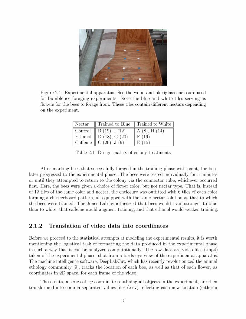
Figure 2.1: Experimental apparatus. See the wood and plexiglass enclosure usedfor bumblebee foraging experiments. Note the blue and white tiles serving asflowers for the bees to forage from. These tiles contain different nectars dependingon the experiment.

Nectar Trained to Blue Trained to White

Control B (19), I (12) A (8), H (14)Ethanol D (18), G (20) F (19)Caffeine C (20), J (9) E (15)

Table 2.1: Design matrix of colony treatments

After marking bees that successfully foraged in the training phase with paint, the beeslater progressed to the experimental phase. The bees were tested individually for 5 minutesor until they attempted to return to the colony via the connector tube, whichever occurredfirst. Here, the bees were given a choice of flower color, but not nectar type. That is, insteadof 12 tiles of the same color and nectar, the enclosure was outfitted with 6 tiles of each colorforming a checkerboard pattern, all equipped with the same nectar solution as that to whichthe bees were trained. The Jones Lab hypothesized that bees would train stronger to bluethan to white, that caffeine would augment training, and that ethanol would weaken training.

2.1.2 Translation of video data into coordinates

Before we proceed to the statistical attempts at modeling the experimental results, it is worthmentioning the logistical task of formatting the data produced in the experimental phasein such a way that it can be analyzed computationally. The raw data are video files (.mp4)taken of the experimental phase, shot from a birds-eye-view of the experimental apparatus.The machine intelligence software, DeepLabCut, which has recently revolutionized the animalethology community [9], tracks the location of each bee, as well as that of each flower, ascoordinates in 2D space, for each frame of the video.

These data, a series of xy-coordinates outlining all objects in the experiment, are thentransformed into comma-separated values files (.csv) reflecting each new location (either a

15

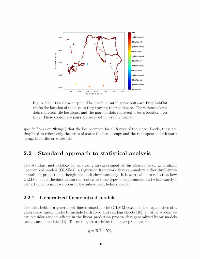
Figure 2.2: Raw data output. The machine intelligence software DeepLabCuttracks the location of the bees as they traverse their enclosure. The various coloreddots represent tile locations, and the maroon dots represent a bee’s location overtime. These coordinate pairs are received in .csv file format.

specific flower or “flying”) that the bee occupies, for all frames of the video. Lastly, these aresimplified to reflect only the series of states the bees occupy and the time spent in each state:flying, blue tile, or white tile.

2.2 Standard approach to statistical analysis

The standard methodology for analyzing an experiment of this class relies on generalizedlinear-mixed models (GLMMs), a regression framework that can analyze either dwell-timesor training proportions, though not both simultaneously. It is worthwhile to reflect on howGLMMs model the data within the context of these types of experiments, and what exactly Iwill attempt to improve upon in the subsequent, holistic model.

2.2.1 Generalized linear-mixed models

The idea behind a generalized linear-mixed model (GLMM) extends the capabilities of ageneralized linear model to include both fixed and random effects [10]. In other words, wecan consider random effects in the linear prediction process that generalized linear modelscannot accommodate [11]. To see this, let us define the linear predictor η as

η = X~β + Y~γ,

16

where X is an N × p matrix of p predictor variables; Y is an N × q matrix of q random-effectvariables; ~β is a p× 1 column vector of fixed-effect regression coefficients; and ~γ is a q × 1column vector of random-effects. But in order to relate this linear predictor to an outcome inour data D, we need a link function, g(·). In order to ensure the regression model, g has theproperty

g(E(D|~β,~γ)) = η,

in reference to the conditional expectation of D given our predictors.

In this context, the relevant random variable is a Poisson GLMM, used in instances ofcount data. Recall the probability mass function of the Poisson distribution,

P(X = k) =λke−λ

k!,

with a corresponding link function defined

g(·) = ln(·).

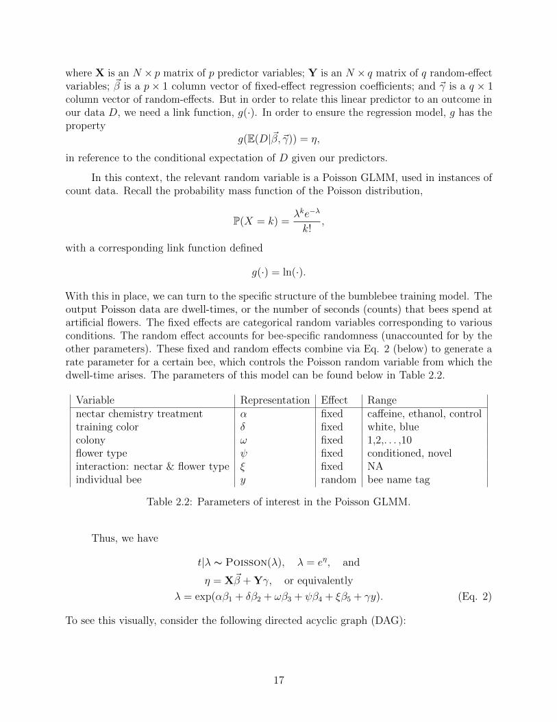
With this in place, we can turn to the specific structure of the bumblebee training model. Theoutput Poisson data are dwell-times, or the number of seconds (counts) that bees spend atartificial flowers. The fixed effects are categorical random variables corresponding to variousconditions. The random effect accounts for bee-specific randomness (unaccounted for by theother parameters). These fixed and random effects combine via Eq. 2 (below) to generate arate parameter for a certain bee, which controls the Poisson random variable from which thedwell-time arises. The parameters of this model can be found below in Table 2.2.

Variable Representation Effect Rangenectar chemistry treatment α fixed caffeine, ethanol, controltraining color δ fixed white, bluecolony ω fixed 1,2,. . . ,10flower type ψ fixed conditioned, novelinteraction: nectar & flower type ξ fixed NAindividual bee y random bee name tag

Table 2.2: Parameters of interest in the Poisson GLMM.

Thus, we have

t|λ ∼ Poisson(λ), λ = eη, and

η = X~β + Yγ, or equivalently

λ = exp(αβ1 + δβ2 + ωβ3 + ψβ4 + ξβ5 + γy). (Eq. 2)

To see this visually, consider the following directed acyclic graph (DAG):

17

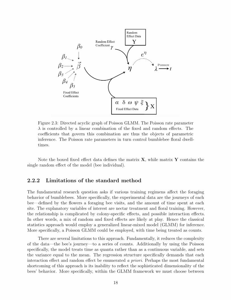
Figure 2.3: Directed acyclic graph of Poisson GLMM. The Poisson rate parameterλ is controlled by a linear combination of the fixed and random effects. Thecoefficients that govern this combination are thus the objects of parametricinference. The Poisson rate parameters in turn control bumblebee floral dwell-times.

Note the boxed fixed effect data defines the matrix X, while matrix Y contains thesingle random effect of the model (bee individual).

2.2.2 Limitations of the standard method

The fundamental research question asks if various training regimens affect the foragingbehavior of bumblebees. More specifically, the experimental data are the journeys of eachbee—defined by the flowers a foraging bee visits, and the amount of time spent at eachsite. The explanatory variables of interest are nectar treatment and floral training. However,the relationship is complicated by colony-specific effects, and possible interaction effects.In other words, a mix of random and fixed effects are likely at play. Hence the classicalstatistics approach would employ a generalized linear-mixed model (GLMM) for inference.More specifically, a Poisson GLMM could be employed, with time being treated as counts.

There are several limitations to this approach. Fundamentally, it reduces the complexityof the data—the bee’s journey—to a series of counts. Additionally by using the Poissonspecifically, the model treats time as quanta rather than as a continuous variable, and setsthe variance equal to the mean. The regression structure specifically demands that eachinteraction effect and random effect be enumerated a priori. Perhaps the most fundamentalshortcoming of this approach is its inability to reflect the sophisticated dimensionality of thebees’ behavior. More specifically, within the GLMM framework we must choose between

18

modeling the dwell-times or the training states, when instead we ought to model themtogether in the same model. To this end, I have developed a hierarchical model to answerthe questions posed by the GLMM regression, without sacrificing the nuance of the foragingdata.

19

Chapter 3

Statistical Model

To overcome the limitations of the GLMM, our model seeks to directly tie the complexityof foraging behavior to the experimental design. How do we answer the questions posed bythe regression: how do the various treatment regimes affect foraging behavior? To this end,I present a hierarchical Bayesian mixture model featuring continuous-time Markov chains.Overall, the complete model consists of three components arranged in a hierarchy, with fullyspecified probability distributions. At the level of the foraging data, I use a continuous-timeMarkov chain model to describe the path that the bees take. At the level of the designmatrix, I employ a logistic regression model to describe the treatment effects. In betweenthese two components, I apply a mixture model structure to stochastically link the results ofthe treatment to the Markov chain. This last piece represents what it means for a bee to besuccessfully trained, or remain untrained. We will now explore each of these pieces of thehierarchy in turn.

3.1 The Journey Model

We begin with two principle assumptions: spatial independence , and memorylessness1.Recalling Figure 2.2, the raw data output consists of a series of coordinates describing a bee’slocation over time. By assuming spatial independence , we assume that the state spacecan be simplified to S = {B,F,W}. That is, a bee must occupy only one of three states:occupying a white flower, occupying a blue tile, or flying between them.

Several factors justify spatial independence. First, the “flowers” are colored tiles thatare identical in every way except for color. Furthermore, each tile of the same color iseffectively indistinguishable from the other members of its class. However, by the nature ofthe experiment, one might suggest that the different locations of each tile within the apparatusrender every individual tile unique. While this may seem relevant at first glance, the sizeof the experiment is small enough that we can expect the bees to not factor this spatialinformation into account. Bumblebees routinely traverse vast distances when foraging, relyingon acute eyesight and olfaction to target and visit different nectar sources [12]. As such,any supposed travel-related, visual, or olfactory disparities between tiles can be reasonablyignored, as they likely do not factor into the bees’ decision-making processes.

1I make a third modeling assumption called training , which is detailed in Chapter 4, section 4.1Transforming the state space.

20

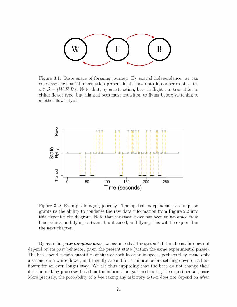
Figure 3.1: State space of foraging journey. By spatial independence, we cancondense the spatial information present in the raw data into a series of statess ∈ S = {W,F,B}. Note that, by construction, bees in flight can transition toeither flower type, but alighted bees must transition to flying before switching toanother flower type.

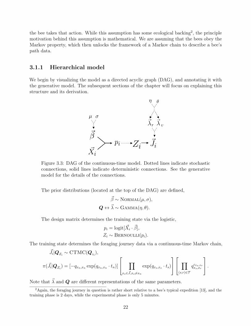
Figure 3.2: Example foraging journey. The spatial independence assumptiongrants us the ability to condense the raw data information from Figure 2.2 intothis elegant flight diagram. Note that the state space has been transformed fromblue, white, and flying to trained, untrained, and flying; this will be explored inthe next chapter.

By assuming memorylessness , we assume that the system’s future behavior does notdepend on its past behavior, given the present state (within the same experimental phase).The bees spend certain quantities of time at each location in space: perhaps they spend onlya second on a white flower, and then fly around for a minute before settling down on a blueflower for an even longer stay. We are thus supposing that the bees do not change theirdecision-making processes based on the information gathered during the experimental phase.More precisely, the probability of a bee taking any arbitrary action does not depend on when

21

the bee takes that action. While this assumption has some ecological backing2, the principlemotivation behind this assumption is mathematical. We are assuming that the bees obey theMarkov property, which then unlocks the framework of a Markov chain to describe a bee’spath data.

3.1.1 Hierarchical model

We begin by visualizing the model as a directed acyclic graph (DAG), and annotating it withthe generative model. The subsequent sections of the chapter will focus on explaining thisstructure and its derivation.

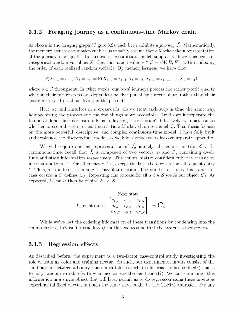
Figure 3.3: DAG of the continuous-time model. Dotted lines indicate stochasticconnections, solid lines indicate deterministic connections. See the generativemodel for the details of the connections.

The prior distributions (located at the top of the DAG) are defined,

~β ∼ Normal(µ, σ),

Q↔ ~λ ∼ Gamma(η, θ).

The design matrix determines the training state via the logistic,

pi = logit[ ~Xi · ~β],

Zi ∼ Bernoulli(pi).

The training state determines the foraging journey data via a continuous-time Markov chain,

~Ji|QZi∼ CTMC(Qzi

),

π( ~Ji|QZi) = [−qxn,xn exp(qxn,xn · tn)]

∏xs∈ ~J,xs 6=xn

exp(qxs,xs · ts)

∏(s,r)∈T

qcxs,xrxs,xr

.Note that ~λ and Q are different representations of the same parameters.

2Again, the foraging journey in question is rather short relative to a bee’s typical expedition [13], and thetraining phase is 2 days, while the experimental phase is only 5 minutes.

22

3.1.2 Foraging journey as a continuous-time Markov chain

As shown in the foraging graph (Figure 3.2), each bee i exhibits a journey ~Ji. Mathematically,the memorylessness assumption enables us to safely assume that a Markov chain representationof the journey is adequate. To construct the statistical model, suppose we have a sequence ofcategorical random variables Xt that can take a value s ∈ S = {W,B, F}, with t indexingthe order of each realized random variable. By memorylessness, we have that

P(Xt+1 = st+1

∣∣Xt = st) = P(Xt+1 = st+1

∣∣Xt = st, Xt−1 = st−1, . . . , X1 = s1),

where s ∈ S throughout. In other words, our bees’ journeys possess the rather poetic qualitywherein their future steps are dependent solely upon their current state, rather than theirentire history. Talk about living in the present!

Here we find ourselves at a crossroads: do we treat each step in time the same way,homogenizing the process and making things more accessible? Or do we incorporate thetemporal dimension more carefully, complicating the situation? Effectively, we must choosewhether to use a discrete- or continuous-time Markov chain to model ~Ji. This thesis focuseson the more powerful, descriptive, and complex continuous-time model. I have fully builtand explained the discrete-time model, as well; it is attached as its own separate appendix.

We will require another representation of ~Ji, namely, the counts matrix, Ci. Incontinuous-time, recall that ~Ji is composed of two vectors, ~ti and ~xi, containing dwell-time and state information respectively. The counts matrix considers only the transitioninformation from ~xi. For all entries a ∈ ~xi except the last, there exists the subsequent entryb. Thus, a → b describes a single class of transition. The number of times this transitionclass occurs in ~xi defines ca,b. Repeating this process for all a, b ∈ S yields our object Ci. Asexpected, Ci must then be of size |S| × |S|:

Next state

Current state

cT,T cT,F cT,NcF,T cF,F cF,NcN,T cN,F cN,N

=C i.

While we’ve lost the ordering information of these transitions by condensing into thecounts matrix, this isn’t a true loss given that we assume that the system is memoryless.

3.1.3 Regression effects

As described before, the experiment is a two-factor case-control study investigating therole of training color and training nectar. As such, our experimental inputs consist of thecombination between a binary random variable (to what color was the bee trained?), and aternary random variable (with what nectar was the bee trained?). We can summarize thisinformation in a single object that will later permit us to do regression using these inputs asexperimental fixed effects, in much the same way sought by the GLMM approach. For any

23

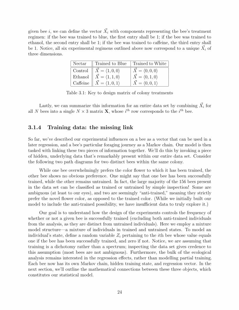
given bee i, we can define the vector ~Xi with components representing the bee’s treatmentregimen: if the bee was trained to blue, the first entry shall be 1; if the bee was trained toethanol, the second entry shall be 1; if the bee was trained to caffeine, the third entry shallbe 1. Notice, all six experimental regimens outlined above now correspond to a unique ~Xi ofthree dimensions.

Nectar Trained to Blue Trained to White

Control ~X = 〈1, 0, 0〉 ~X = 〈0, 0, 0〉Ethanol ~X = 〈1, 1, 0〉 ~X = 〈0, 1, 0〉Caffeine ~X = 〈1, 0, 1〉 ~X = 〈0, 0, 1〉

Table 3.1: Key to design matrix of colony treatments

Lastly, we can summarize this information for an entire data set by combining ~Xi forall N bees into a single N × 3 matrix X, whose ith row corresponds to the ith bee.

3.1.4 Training data: the missing link

So far, we’ve described our experimental influences on a bee as a vector that can be used in alater regression, and a bee’s particular foraging journey as a Markov chain. Our model is thentasked with linking these two pieces of information together. We’ll do this by invoking a pieceof hidden, underlying data that’s remarkably present within our entire data set. Considerthe following two path diagrams for two distinct bees within the same colony.

While one bee overwhelmingly prefers the color flower to which it has been trained, theother bee shows no obvious preference. One might say that one bee has been successfullytrained, while the other remains untrained. In fact, the large majority of the 156 bees presentin the data set can be classified as trained or untrained by simple inspection! Some areambiguous (at least to our eyes), and two are seemingly “anti-trained,” meaning they strictlyprefer the novel flower color, as opposed to the trained color. (While we initially built ourmodel to include the anti-trained possibility, we have insufficient data to truly explore it.)

Our goal is to understand how the design of the experiments controls the frequency ofwhether or not a given bee is successfully trained (excluding both anti-trained individualsfrom the analysis, as they are distinct from untrained individuals). Here we employ a mixturemodel structure—a mixture of individuals in trained and untrained states. To model anindividual’s state, define a random variable Zi pertaining to the ith bee whose value equalsone if the bee has been successfully trained, and zero if not. Notice, we are assuming thattraining is a dichotomy rather than a spectrum; inspecting the data set gives credence tothis assumption (most bees are not ambiguous). Furthermore, the bulk of the ecologicalanalysis remains interested in the regression effects, rather than modelling partial training.Each bee now has its own Markov chain, hidden training state, and regression vector. In thenext section, we’ll outline the mathematical connections between these three objects, whichconstitutes our statistical model.

24

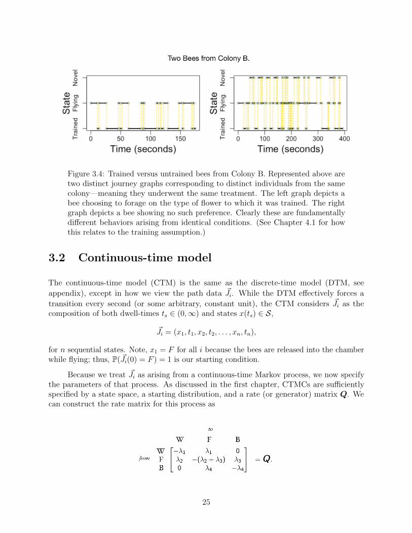
Figure 3.4: Trained versus untrained bees from Colony B. Represented above aretwo distinct journey graphs corresponding to distinct individuals from the samecolony—meaning they underwent the same treatment. The left graph depicts abee choosing to forage on the type of flower to which it was trained. The rightgraph depicts a bee showing no such preference. Clearly these are fundamentallydifferent behaviors arising from identical conditions. (See Chapter 4.1 for howthis relates to the training assumption.)

3.2 Continuous-time model

The continuous-time model (CTM) is the same as the discrete-time model (DTM, see

appendix), except in how we view the path data ~Ji. While the DTM effectively forces a

transition every second (or some arbitrary, constant unit), the CTM considers ~Ji as thecomposition of both dwell-times ts ∈ (0,∞) and states x(ts) ∈ S,

~Ji = (x1, t1, x2, t2, . . . , xn, tn),

for n sequential states. Note, x1 = F for all i because the bees are released into the chamberwhile flying; thus, P( ~Ji(0) = F ) = 1 is our starting condition.

Because we treat ~Ji as arising from a continuous-time Markov process, we now specifythe parameters of that process. As discussed in the first chapter, CTMCs are sufficientlyspecified by a state space, a starting distribution, and a rate (or generator) matrix Q. Wecan construct the rate matrix for this process as

25

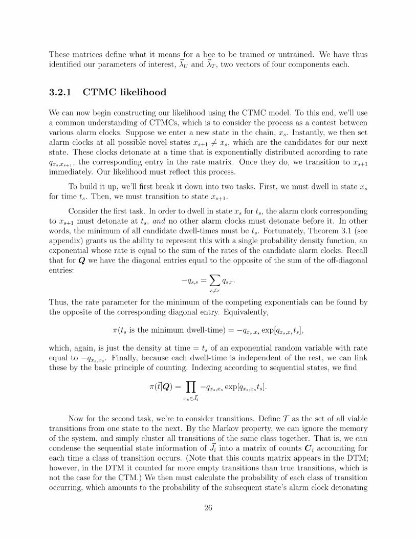
These matrices define what it means for a bee to be trained or untrained. We have thusidentified our parameters of interest, ~λU and ~λT , two vectors of four components each.

3.2.1 CTMC likelihood

We can now begin constructing our likelihood using the CTMC model. To this end, we’ll usea common understanding of CTMCs, which is to consider the process as a contest betweenvarious alarm clocks. Suppose we enter a new state in the chain, xs. Instantly, we then setalarm clocks at all possible novel states xs+1 6= xs, which are the candidates for our nextstate. These clocks detonate at a time that is exponentially distributed according to rateqxs,xs+1 , the corresponding entry in the rate matrix. Once they do, we transition to xs+1

immediately. Our likelihood must reflect this process.

To build it up, we’ll first break it down into two tasks. First, we must dwell in state xsfor time ts. Then, we must transition to state xs+1.

Consider the first task. In order to dwell in state xs for ts, the alarm clock correspondingto xs+1 must detonate at ts, and no other alarm clocks must detonate before it. In otherwords, the minimum of all candidate dwell-times must be ts. Fortunately, Theorem 3.1 (seeappendix) grants us the ability to represent this with a single probability density function, anexponential whose rate is equal to the sum of the rates of the candidate alarm clocks. Recallthat for Q we have the diagonal entries equal to the opposite of the sum of the off-diagonalentries:

−qs,s =∑s 6=r

qs,r.

Thus, the rate parameter for the minimum of the competing exponentials can be found bythe opposite of the corresponding diagonal entry. Equivalently,

π(ts is the minimum dwell-time) = −qxs,xs exp[qxs,xsts],

which, again, is just the density at time = ts of an exponential random variable with rateequal to −qxs,xs . Finally, because each dwell-time is independent of the rest, we can linkthese by the basic principle of counting. Indexing according to sequential states, we find

π(~t|Q) =∏xs∈ ~Ji

−qxs,xs exp[qxs,xsts].

Now for the second task, we’re to consider transitions. Define T as the set of all viabletransitions from one state to the next. By the Markov property, we can ignore the memoryof the system, and simply cluster all transitions of the same class together. That is, we cancondense the sequential state information of ~Ji into a matrix of counts Ci accounting foreach time a class of transition occurs. (Note that this counts matrix appears in the DTM;however, in the DTM it counted far more empty transitions than true transitions, which isnot the case for the CTM.) We then must calculate the probability of each class of transitionoccurring, which amounts to the probability of the subsequent state’s alarm clock detonating

26

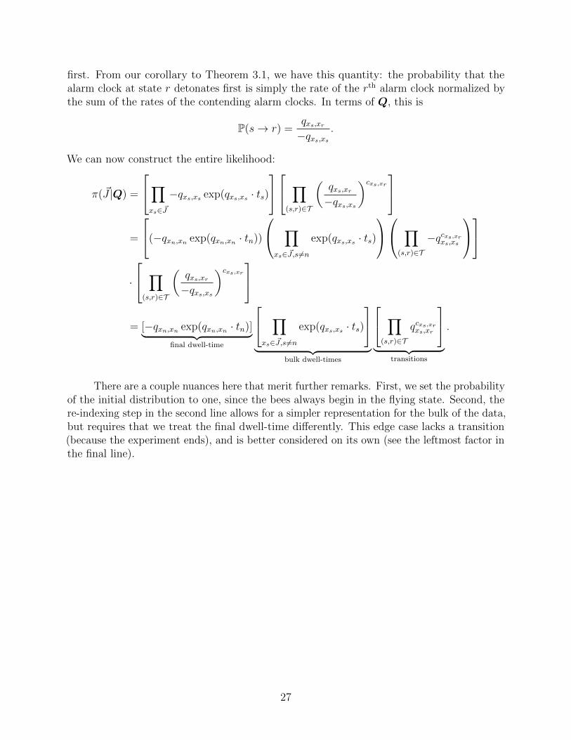
first. From our corollary to Theorem 3.1, we have this quantity: the probability that thealarm clock at state r detonates first is simply the rate of the rth alarm clock normalized bythe sum of the rates of the contending alarm clocks. In terms of Q, this is

P(s→ r) =qxs,xr−qxs,xs

.

We can now construct the entire likelihood:

π( ~J |Q) =

∏xs∈ ~J

−qxs,xs exp(qxs,xs · ts)

∏(s,r)∈T

(qxs,xr−qxs,xs

)cxs,xr=

(−qxn,xn exp(qxn,xn · tn))

∏xs∈ ~J,s6=n

exp(qxs,xs · ts)

∏(s,r)∈T

−qcxs,xrxs,xs

·

∏(s,r)∈T

(qxs,xr−qxs,xs

)cxs,xr= [−qxn,xn exp(qxn,xn · tn)]︸ ︷︷ ︸

final dwell-time

∏xs∈ ~J,s6=n

exp(qxs,xs · ts)

︸ ︷︷ ︸

bulk dwell-times

∏(s,r)∈T

qcxs,xrxs,xr

︸ ︷︷ ︸

transitions

.

There are a couple nuances here that merit further remarks. First, we set the probabilityof the initial distribution to one, since the bees always begin in the flying state. Second, there-indexing step in the second line allows for a simpler representation for the bulk of the data,but requires that we treat the final dwell-time differently. This edge case lacks a transition(because the experiment ends), and is better considered on its own (see the leftmost factor inthe final line).

27

Chapter 4

Inference

The following algorithm contains various flavors of the Metropolis-Hastings Algorithm, asper my discussion in Chapter 1. According to the model, the regression and journey processparameters are always conditionally independent of each other, given the training state.This allows us to completely ignore the regression parameters when updating the journeyprocess parameters, provided we have the training information (and vice-versa). Furthermore,the training posteriors are automatically defined when we condition upon both the journeyprocess and regression parameters. So, while the training state might be a hidden variable, itmakes sampling much more accessible.

Note that all inference was accomplished using the open source statistical programminglanguage R [14]. Many plots are made possible by the ggplot2 environment from HadleyWickham’s tidyverse [15].

4.1 Transforming the state space

When coding the algorithm, we have to be slightly more specific in what we mean by“trained.” Recall that all of our state spaces thus far have been explicitly defined as {W,F,B},representing the two flower types and flight. Recall further that each bee was exposed toeither blue or white in the training phase. As such, we want our Markov chains to actuallymodel the training states, rather than what flower the bee is on, because that’s what the restof the model seeks to explain. To that end, we perform a mapping from S ∈ {B,F,W} toS ′ ∈ {T, F,N}, before running the algorithm. These states are trained (the flower color ofthe training phase), flying, or novel (the opposite flower color of the training phase). (Wecould also refer to the novel state as the “antitrained” state, in honor of the two renegadebees that actively disobeyed their training.) This allows us to format all Markov chains (andthus all transition, Dirichlet, and rate matrices, in both discrete- and continuous-time) suchthat each state is assigned a sequential index (T = 1, F = 2, N = 3). I refer to this mappingas the third assumption of the model, the training assumption, and puts figure 3.4 in bettercontext.

4.2 Continuous-Time Markov chain inference

The algorithm is broken down into update routines that attempt to sample from the conditionalposterior of each variable class. Careful tempering and ordering aid convergence.

28

4.2.1 Move 1: Metropolis-Hastings sampling of regression coeffi-cients

When it comes to updating the regression coefficients ~β, no conjugacy comes readily tomind. As such, we must recourse to the computationally slower (but still revolutionary!)Metropolis-Metropolis-Hastings algorithm of 1970. Again, our goal is to sample from themarginal posterior distribution of (~β|X, ~λ, ~Z), which can be simplified to (~β|X, ~Z) by theaforementioned conditional independence structure. Recalling the key to the design matrixfrom Chapter 2, there are three weight parameters and one intercept parameter that need tobe sampled (two binary, one ternary variable in this logistic regression).

Recall the explanation of the MHA in the first chapter. At the heart of the MHA wehave the MH ratio, used in the expression

A = min

(1,π∗(x′t+1)Q(xt|x′t+1)

π∗(xt)Q(x′t+1|xt)

),

where π∗ refers to a target distribution, and Q refers to the proposal distribution (sometimesreferred to as a transition kernel). Additionally, note that x′t+1 has merely been proposedfrom Q, rather than being installed in the chain (hence the prime demarcation). In thiscase, our target distribution is the posterior, and our proposal distribution is a normaldistribution, seeing as the parameters of interest are real numbers. For example, Q(xt|x′t+1)takes the density of a normal distribution with mean xt+1 and standard deviation equal toour predetermined walk parameter. To represent the target posterior distribution, we applyBayes’s Law,

π∗(x′t+1)

π∗(xt)=π(~β′t+1|X, ~Z)

π(~βt|X, ~Z)

=π(~Z|~β′t+1,X)π(~β′t+1)

π(X)÷ π(~Z|~βt,X)π(~βt)

π(X)

=π(~Z|~β′t+1,X)π(~β′t+1)

π(~Z|~βt,X)π(~βt)

=

[∏i logit(~β′t+1 ·X)Zi(1− logit(~β′t+1 ·X))1−Z1

] [∏k

exp[−(β′k,t+1−µk)2/(2σ2

k)]

σk√

2π

][∏

i logit(~β′t ·X)Zi(1− logit(~β′t ·X))1−Z1

] [∏k

exp[−(β′k,t−µk)2/(2σ2

k)]

σk√

2π

] ,

where i indexes each bee, and k each ~β component. Note, the two prior distributions (π(~β))simply obey the density of a normal distribution, with predetermined mean µk and standarddeviation σk defined for each component of ~β. The likelihood refers to i independent Bernoullioutcomes weighted according to pi = logit( ~Xi · ~β). Clearly, this ratio is readily computable

when conditioned upon ~Z.

With this ratio calculated, we accept the proposal state ~β′t+1 as ~βt+1 with probability A.(Note, the minimum statement simply prevents the probability from exceeding unity.)

29

4.2.2 Move 2: Metropolis-Hastings sampling of rate matrix pa-rameters

Recall from the hierarchical model that each of the two rate matrices is defined by fourrate parameters, denoted ~λZi

∈ {~λT , ~λU} with ~λ ∈ R4>0. We then have eight parameters to

find, with no conjugacy relationship to aid our search. As such, we recourse to Metropolis-Hastings, using our likelihood from the previous chapter, and Gamma(shape = 1.5, rate= 1.5) distributions for our priors on each. (Note, the prior for the real data runs is morenuanced, as I discuss in the next section.)

For the proposal distribution, we have to be careful that the proposed parameters donot become negative (the domain of an exponential random variable is strictly positive).Instead of using a normally distributed random walk with the old parameter set as the mean(as is done in the discrete-time case), we’ll use a proportionality-based variant that avoidsproposing non-positive parameters. We draw a scale factor R from

R ∼ Uniform

(x

1 + x,1 + x

x

),

and multiply it by the current λ to yield the proposed update. The key here is that theHastings ratio is symmetric; in other words, the probability of proposing state Θi from Θj

doesn’t change if we swap i and j. We found that x = 3 aids convergence.

4.2.3 Move 3: Training state posterior calculation

In the case where we hold the rate matrix and regression parameters constant, we can samplefrom the training state posterior directly. First, recall that because Zi ∼ Bernoulli(pi),there are only two possible outcomes of Zi, denoted m ∈ {Trained,Untrained}. As such,the Law of Total Probability enables direct posterior sampling: we know the likelihood andprior of both possible states, which defines an unnormalized posterior (it lacks the marginal,which is the normalizing constant from Bayes’s Law). Then, by dividing through with theiraggregate, we can find the posterior up to a constant.

To that end, we must consider the prior and likelihood. The prior is simply the underlyingprobability of training given the treatment regimen. The likelihood is the probability of thejourney data occurring if it is distributed as a continuous-time Markov chain with rate matrixQ. (For ease of reading, we group ~Ji, Ci, and ~Xi as data D; and we use Q to represent boththe trained and untrained matrices). We can see all this mathematically as

π(Zi = m|D, ~β,Q)︸ ︷︷ ︸posterior

∝∑∀m

(π( ~Ji|Qm)︸ ︷︷ ︸

likelihood

· π(Zi = m| ~Xi, ~β)︸ ︷︷ ︸prior

)

∝ L( ~Ji|QT ) ·(

logit( ~Xi · ~β)︸ ︷︷ ︸pi

)+ L( ~Ji|QU) ·

(1− logit( ~Xi · ~β)︸ ︷︷ ︸

1−pi

),

30

where the likelihood, as derived in Chapter 3, is

L( ~Ji|Q) =

∏s∈ ~J

−qs,s exp(qs,s · ts)

∏(s,r)∈T

(qs,r−qs,s

)cs,r ,where we simplify the notation by replacing xs with just s.

Because we’ve defined all states that the unnormalized posterior can take, we cannormalize these states by dividing through with their sum. Thus, for an example of one ofthe posterior probabilities, consider the probability of being trained:

π(Zi = T |D, ~β,Q) =

L( ~Ji|QT ) ·(

logit( ~Xi · ~β)

)[L( ~Ji|QT ) ·

(logit( ~Xi · ~β)

)]+

[L( ~Ji|QU) ·

(1− logit( ~Xi · ~β)

)]

=

∏s∈ ~J

−qT,s,s exp(qT,s,s · ts)

∏(s,r)∈T

(qT,s,r−qT,s,s

)cs,r · (logit( ~Xi · ~β))

÷

(∏s∈ ~J

−qT,s,s exp(qT,s,s · ts)

∏(s,r)∈T

(qT,s,r−qT,s,s

)cs,r · (logit( ~Xi · ~β))

+

∏s∈ ~J

−qU,s,s exp(qU,s,s · ts)

∏(s,r)∈T

(qU,s,r−qU,s,s

)cs,r · (1− logit( ~Xi · ~β)))

.

We’ve thus fully specified the posterior distribution for the training state. By evaluating thisexpression, we find the posterior probabilities of training versus untraining, which then makesupdating ~Z equivalent to a series of weighted coin tosses.

4.2.4 Compound CTM Algorithm

Each of the three classes of moves requires that we condition upon one of the three majorvariables that we seek to update. As such, the algorithm proceeds in a step-wise manner,doing exactly one of the moves for each next step. The order and frequency of these moves isup to us. This—along with tuning parameters like priors and proposal dispersion—is wherescience becomes art.

To set up the algorithm, we must define all parameters for each prior distribution.For the regression coefficients, ~β ∈ R4. These can, in theory, be any real number, but thelogistic likelihood becomes zero for many combinations; after some experimentation, we usednormal distributions with mean = 0 and standard deviation = 8 for all four components. Therate matrix parameters ~λ must be greater than zero for the exponential to be defined, thatis λ ∈ R>0. We employ the disperse Gamma(1.5, 1.5) generally, but take a more nuancedapproach for the real data.

31

For the real data, I have crafted a more involved, data-related prior structure. TheCTM has trouble converging to a sensibly separated mixture on its own. In other words, itfrequently collapses into a state where all bees are identically trained, or eventually sticksto a local mode wherein the majority of bees are not sensibly classified. To combat theseproblems, I reflected on what prior information we have that wasn’t being included in themodel.

By using a process known as tempering the chain, we can hone the parameters to asomewhat reasonable place very rapidly, before letting the chain freely update. We do thisby ignoring one of the three parameter classes. By ignoring the regression coefficients, wecan ask the Q and ~Z parameters to come to some reasonable agreement independently ofthe regression; similarly, by ignoring the rate matrices, we can ask the ~β and ~Z parametersto come to some sort of agreement. Then, when we run the chain with these parameterstogether, each parameter will have a far more reasonable starting position, which cuts downon computation time significantly.

According to the exploratory data analysis, most bees clearly occupy either a trained oruntrained state, which we can identify graphically. If we could represent those states in termsof CTMC rate matrices, we could inform our prior distribution on ~λ accordingly. To thatend, I selected two sets of bees (that I’ll call training set candidates) that appeared, by eye,to be unequivocally either trained or untrained. I further limited the selection to bees thatperformed at least 20 transitions (relatively high data quality). Of the 154 bees in total, 22trained and 40 untrained bees met this criteria. I then ran 10 parallel chains in the followingfashion: 10 bees from each training set were randomly sampled and treated as fixed. Then,2,000 rate matrix MH moves were run, and the last quarter were stored. Looking over theten runs, the convergence was consistent enough (even across different training sets!) to usethese matrices as the priors. Effectively, these values informed the shape and rate parametersof our prior gamma distribution (details in the appendix for Chapter 6). This obviated the

need for a Q-~Z tempering process and label switching check1 in the full, real data runs. Note,the ~β − ~Z pair was still tempered.

Because of the prior search procedure, the regression coefficients are updated threetimes as frequently as the other two parameter classes, with ~λ being updated 2.5 times morefrequently than ~Z (due to the variability in a random-walk MH).

4.3 Convergence

Each run consisted of two thousand tempering iterations, followed by 200,000 unconstrainediterations. The algorithm recorded one out of every 500 states to increase storage efficiencyand reduce autocorrelation (see plots below). I ran ten chains in parallel for an effective

sample size of roughly 8,000 per ~β component (with similarly large values for the otherparameters). Across all chains, I found specific convergence to a single mode, with the medianposterior samples for each independent runs being similar.

1See details of the discrete-time inference algorithm for a discussion of the label-switching problem [16].

32

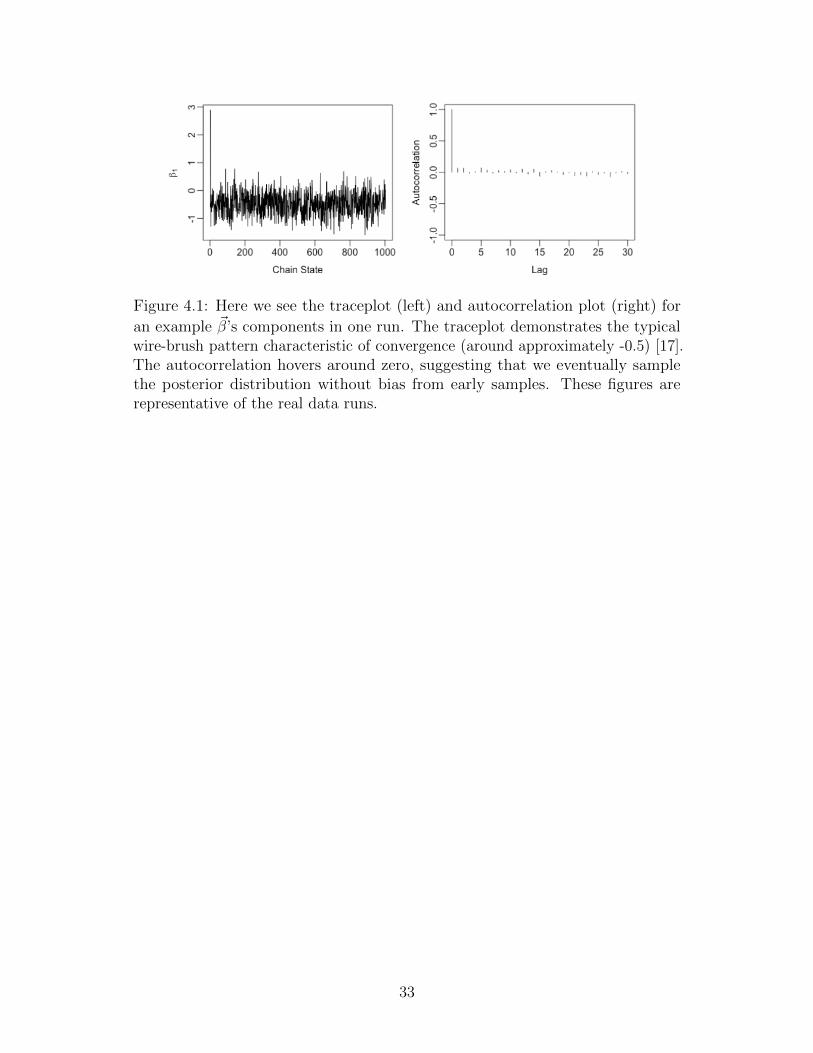
Figure 4.1: Here we see the traceplot (left) and autocorrelation plot (right) for

an example ~β’s components in one run. The traceplot demonstrates the typicalwire-brush pattern characteristic of convergence (around approximately -0.5) [17].The autocorrelation hovers around zero, suggesting that we eventually samplethe posterior distribution without bias from early samples. These figures arerepresentative of the real data runs.

33

Chapter 5

Simulation Studies

Before we apply the model to the experimental data, we want to have some understandingof and confidence in its ability to infer a variety of hypothetical parameters given the sizeof our datasets. To accomplish this, we employ simulation studies, where we simulate dataaccording to the hierarchical model with known parameters of our own choosing, and thenattempt to retrieve those parameters using the model. Obviously, we will not tell the modelthe true parameters; instead, we will assume knowledge of only priors, and use the inferencealgorithm to find the values.

Since we aim to generate hypothetical data according to the model, we need to definethe parameters governing the underlying process. Recall that the regression parameterscontrol the training probabilities as a function of the experimental design, and the rate matrixparameters control the journeys. With this in mind, consider the following simulation routine:

1. Define an underlying regression vector that, through experimentation, yields stableinference:

βintercept βblue βEtOH βcaff

-0.74 1.5 -1.5 0.02

Table 5.1: Hypothetical regression vector for simulation studies

2. Assign randomly generated regression effects ~X to each of the N bees. We now have afully defined pi for each bee i, as pi = logit(~β · ~Xi).

3. Simulate one Bernoulli random variable weighted pi for each of the N bees: this amountsto assigning the bees their underlying training status.

4. Define what those training statuses imply by specifying two rate matrices, QU and QT .

5. For each bee, simulate a continuous-time Markov chain journey according to QZi(the

relevant rate matrix, as determined by the training status). These journeys are (atleast) t seconds long1.

The algorithm receives only the simulated ~Ji and ~Xi information (reflecting realistic condi-

tions), and is tasked to infer Q, ~β, and ~Z.

1The CTMC simulation routine requires a minimum total flight duration. When adding a dwell-timewould exceed this threshold, the time and subsequent transition are still recorded, but the journey ceases.

34

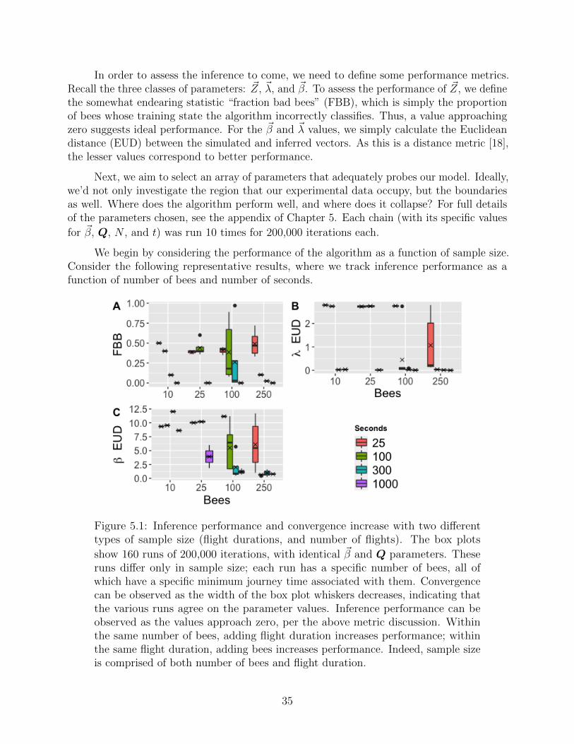
In order to assess the inference to come, we need to define some performance metrics.Recall the three classes of parameters: ~Z, ~λ, and ~β. To assess the performance of ~Z, we definethe somewhat endearing statistic “fraction bad bees” (FBB), which is simply the proportionof bees whose training state the algorithm incorrectly classifies. Thus, a value approachingzero suggests ideal performance. For the ~β and ~λ values, we simply calculate the Euclideandistance (EUD) between the simulated and inferred vectors. As this is a distance metric [18],the lesser values correspond to better performance.

Next, we aim to select an array of parameters that adequately probes our model. Ideally,we’d not only investigate the region that our experimental data occupy, but the boundariesas well. Where does the algorithm perform well, and where does it collapse? For full detailsof the parameters chosen, see the appendix of Chapter 5. Each chain (with its specific values

for ~β, Q, N , and t) was run 10 times for 200,000 iterations each.

We begin by considering the performance of the algorithm as a function of sample size.Consider the following representative results, where we track inference performance as afunction of number of bees and number of seconds.

Figure 5.1: Inference performance and convergence increase with two differenttypes of sample size (flight durations, and number of flights). The box plots

show 160 runs of 200,000 iterations, with identical ~β and Q parameters. Theseruns differ only in sample size; each run has a specific number of bees, all ofwhich have a specific minimum journey time associated with them. Convergencecan be observed as the width of the box plot whiskers decreases, indicating thatthe various runs agree on the parameter values. Inference performance can beobserved as the values approach zero, per the above metric discussion. Withinthe same number of bees, adding flight duration increases performance; withinthe same flight duration, adding bees increases performance. Indeed, sample sizeis comprised of both number of bees and flight duration.

35

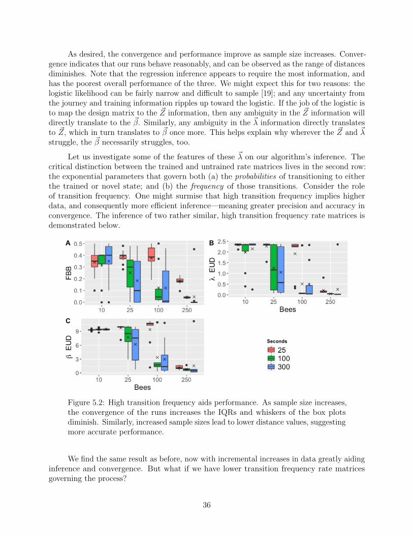
As desired, the convergence and performance improve as sample size increases. Conver-gence indicates that our runs behave reasonably, and can be observed as the range of distancesdiminishes. Note that the regression inference appears to require the most information, andhas the poorest overall performance of the three. We might expect this for two reasons: thelogistic likelihood can be fairly narrow and difficult to sample [19]; and any uncertainty fromthe journey and training information ripples up toward the logistic. If the job of the logistic isto map the design matrix to the ~Z information, then any ambiguity in the ~Z information willdirectly translate to the ~β. Similarly, any ambiguity in the ~λ information directly translatesto ~Z, which in turn translates to ~β once more. This helps explain why wherever the ~Z and ~λstruggle, the ~β necessarily struggles, too.

Let us investigate some of the features of these ~λ on our algorithm’s inference. Thecritical distinction between the trained and untrained rate matrices lives in the second row:the exponential parameters that govern both (a) the probabilities of transitioning to eitherthe trained or novel state; and (b) the frequency of those transitions. Consider the roleof transition frequency. One might surmise that high transition frequency implies higherdata, and consequently more efficient inference—meaning greater precision and accuracy inconvergence. The inference of two rather similar, high transition frequency rate matrices isdemonstrated below.

Figure 5.2: High transition frequency aids performance. As sample size increases,the convergence of the runs increases the IQRs and whiskers of the box plotsdiminish. Similarly, increased sample sizes lead to lower distance values, suggestingmore accurate performance.

We find the same result as before, now with incremental increases in data greatly aidinginference and convergence. But what if we have lower transition frequency rate matricesgoverning the process?

36

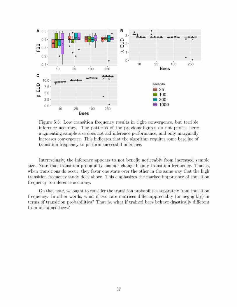
Figure 5.3: Low transition frequency results in tight convergence, but terribleinference accuracy. The patterns of the previous figures do not persist here:augmenting sample size does not aid inference performance, and only marginallyincreases convergence. This indicates that the algorithm requires some baseline oftransition frequency to perform successful inference.

Interestingly, the inference appears to not benefit noticeably from increased samplesize. Note that transition probability has not changed: only transition frequency. That is,when transitions do occur, they favor one state over the other in the same way that the hightransition frequency study does above. This emphasizes the marked importance of transitionfrequency to inference accuracy.

On that note, we ought to consider the transition probabilities separately from transitionfrequency. In other words, what if two rate matrices differ appreciably (or negligibly) interms of transition probabilities? That is, what if trained bees behave drastically differentfrom untrained bees?

37

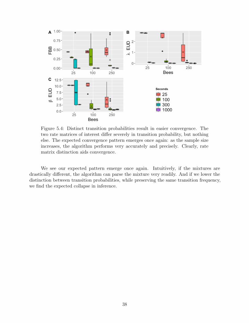
Figure 5.4: Distinct transition probabilities result in easier convergence. Thetwo rate matrices of interest differ severely in transition probability, but nothingelse. The expected convergence pattern emerges once again: as the sample sizeincreases, the algorithm performs very accurately and precisely. Clearly, ratematrix distinction aids convergence.

We see our expected pattern emerge once again. Intuitively, if the mixtures aredrastically different, the algorithm can parse the mixture very readily. And if we lower thedistinction between transition probabilities, while preserving the same transition frequency,we find the expected collapse in inference.

38

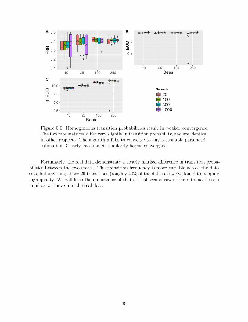
Figure 5.5: Homogeneous transition probabilities result in weaker convergence.The two rate matrices differ very slightly in transition probability, and are identicalin other respects. The algorithm fails to converge to any reasonable parametricestimation. Clearly, rate matrix similarity harms convergence.

Fortunately, the real data demonstrate a clearly marked difference in transition proba-bilities between the two states. The transition frequency is more variable across the datasets, but anything above 20 transitions (roughly 40% of the data set) we’ve found to be quitehigh quality. We will keep the importance of that critical second row of the rate matrices inmind as we move into the real data.

39

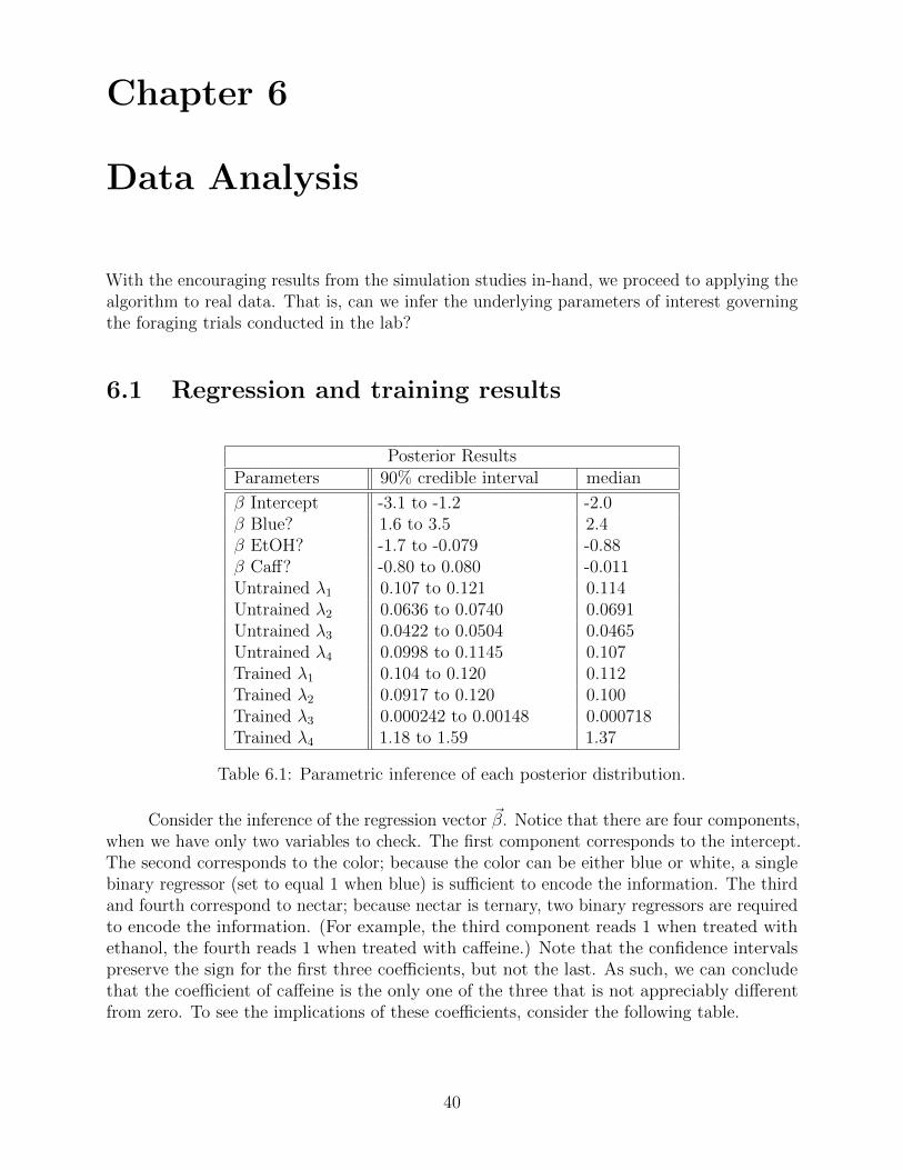
Chapter 6

Data Analysis

With the encouraging results from the simulation studies in-hand, we proceed to applying thealgorithm to real data. That is, can we infer the underlying parameters of interest governingthe foraging trials conducted in the lab?

6.1 Regression and training results

Posterior ResultsParameters 90% credible interval median

β Intercept -3.1 to -1.2 -2.0β Blue? 1.6 to 3.5 2.4β EtOH? -1.7 to -0.079 -0.88β Caff? -0.80 to 0.080 -0.011Untrained λ1 0.107 to 0.121 0.114Untrained λ2 0.0636 to 0.0740 0.0691Untrained λ3 0.0422 to 0.0504 0.0465Untrained λ4 0.0998 to 0.1145 0.107Trained λ1 0.104 to 0.120 0.112Trained λ2 0.0917 to 0.120 0.100Trained λ3 0.000242 to 0.00148 0.000718Trained λ4 1.18 to 1.59 1.37

Table 6.1: Parametric inference of each posterior distribution.

Consider the inference of the regression vector ~β. Notice that there are four components,when we have only two variables to check. The first component corresponds to the intercept.The second corresponds to the color; because the color can be either blue or white, a singlebinary regressor (set to equal 1 when blue) is sufficient to encode the information. The thirdand fourth correspond to nectar; because nectar is ternary, two binary regressors are requiredto encode the information. (For example, the third component reads 1 when treated withethanol, the fourth reads 1 when treated with caffeine.) Note that the confidence intervalspreserve the sign for the first three coefficients, but not the last. As such, we can concludethat the coefficient of caffeine is the only one of the three that is not appreciably differentfrom zero. To see the implications of these coefficients, consider the following table.

40

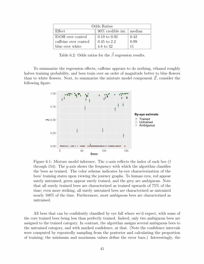
Odds RatiosEffect 90% credible int. median

EtOH over control 0.19 to 0.92 0.42caffeine over control 0.45 to 2.2 0.99blue over white 4.8 to 32 11

Table 6.2: Odds ratios for the ~β regression results.

To summarize the regression effects, caffeine appears to do nothing, ethanol roughlyhalves training probability, and bees train over an order of magnitude better to blue flowersthan to white flowers. Next, to summarize the mixture model component ~Z, consider thefollowing figure.

Figure 6.1: Mixture model inference. The x-axis reflects the index of each bee (1through 154). The y-axis shows the frequency with which the algorithm classifiesthe bees as trained. The color scheme indicates by-eye characterization of thebees’ training states upon viewing the journey graphs. To human eyes, red appearsurely untrained, green appear surely trained, and the grey are ambiguous. Notethat all surely trained bees are characterized as trained upwards of 75% of thetime; even more striking, all surely untrained bees are characterized as untrainednearly 100% of the time. Furthermore, most ambiguous bees are characterized asuntrained.

All bees that can be confidently classified by eye fall where we’d expect, with some ofthe core trained bees being less than perfectly trained. Indeed, only two ambiguous bees areassigned to the trained category. In contrast, the algorithm assigns several ambiguous bees tothe untrained category, and with marked confidence, at that. (Note the confidence intervalswere computed by repeatedly sampling from the posterior and calculating the proportionof training; the minimum and maximum values define the error bars.) Interestingly, the

41

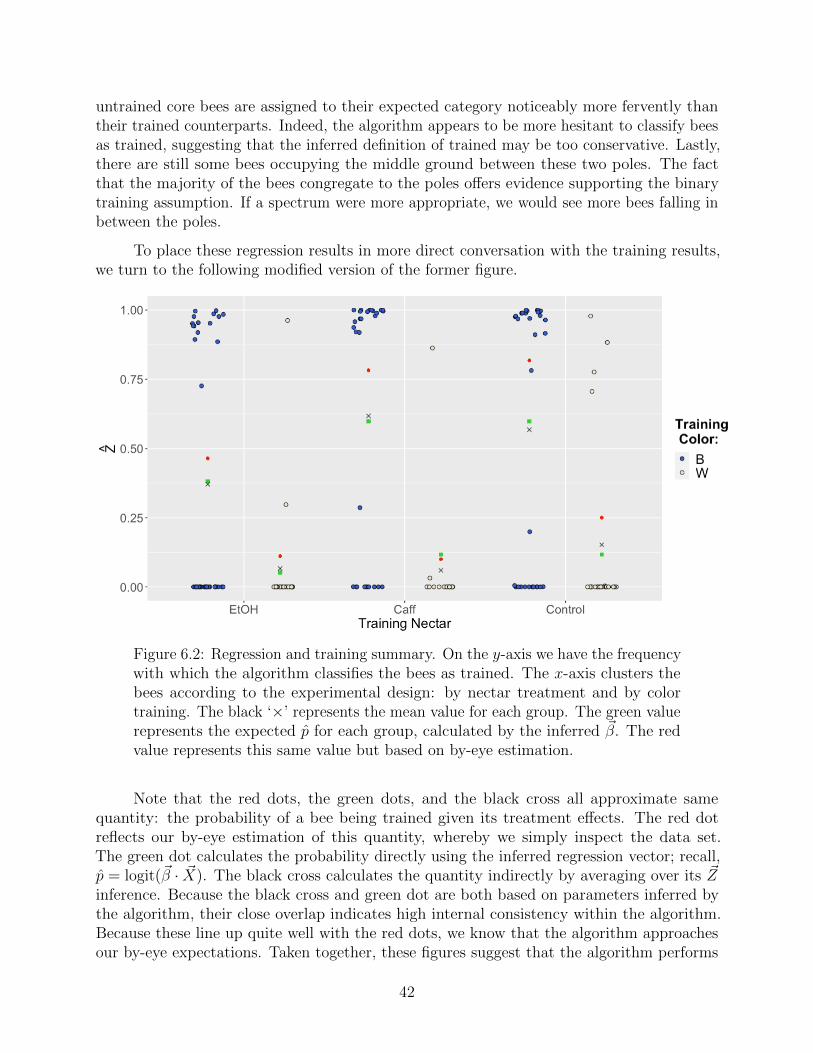
untrained core bees are assigned to their expected category noticeably more fervently thantheir trained counterparts. Indeed, the algorithm appears to be more hesitant to classify beesas trained, suggesting that the inferred definition of trained may be too conservative. Lastly,there are still some bees occupying the middle ground between these two poles. The factthat the majority of the bees congregate to the poles offers evidence supporting the binarytraining assumption. If a spectrum were more appropriate, we would see more bees falling inbetween the poles.

To place these regression results in more direct conversation with the training results,we turn to the following modified version of the former figure.

Figure 6.2: Regression and training summary. On the y-axis we have the frequencywith which the algorithm classifies the bees as trained. The x-axis clusters thebees according to the experimental design: by nectar treatment and by colortraining. The black ‘×’ represents the mean value for each group. The green valuerepresents the expected p̂ for each group, calculated by the inferred ~β. The redvalue represents this same value but based on by-eye estimation.

Note that the red dots, the green dots, and the black cross all approximate samequantity: the probability of a bee being trained given its treatment effects. The red dotreflects our by-eye estimation of this quantity, whereby we simply inspect the data set.The green dot calculates the probability directly using the inferred regression vector; recall,p̂ = logit(~β · ~X). The black cross calculates the quantity indirectly by averaging over its ~Zinference. Because the black cross and green dot are both based on parameters inferred bythe algorithm, their close overlap indicates high internal consistency within the algorithm.Because these line up quite well with the red dots, we know that the algorithm approachesour by-eye expectations. Taken together, these figures suggest that the algorithm performs

42

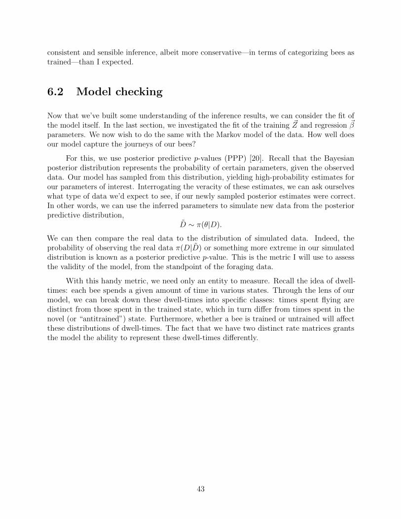
consistent and sensible inference, albeit more conservative—in terms of categorizing bees astrained—than I expected.

6.2 Model checking

Now that we’ve built some understanding of the inference results, we can consider the fit ofthe model itself. In the last section, we investigated the fit of the training ~Z and regression ~βparameters. We now wish to do the same with the Markov model of the data. How well doesour model capture the journeys of our bees?

For this, we use posterior predictive p-values (PPP) [20]. Recall that the Bayesianposterior distribution represents the probability of certain parameters, given the observeddata. Our model has sampled from this distribution, yielding high-probability estimates forour parameters of interest. Interrogating the veracity of these estimates, we can ask ourselveswhat type of data we’d expect to see, if our newly sampled posterior estimates were correct.In other words, we can use the inferred parameters to simulate new data from the posteriorpredictive distribution,

D̃ ∼ π(θ|D).

We can then compare the real data to the distribution of simulated data. Indeed, theprobability of observing the real data π(D|D̃) or something more extreme in our simulateddistribution is known as a posterior predictive p-value. This is the metric I will use to assessthe validity of the model, from the standpoint of the foraging data.

With this handy metric, we need only an entity to measure. Recall the idea of dwell-times: each bee spends a given amount of time in various states. Through the lens of ourmodel, we can break down these dwell-times into specific classes: times spent flying aredistinct from those spent in the trained state, which in turn differ from times spent in thenovel (or “antitrained”) state. Furthermore, whether a bee is trained or untrained will affectthese distributions of dwell-times. The fact that we have two distinct rate matrices grantsthe model the ability to represent these dwell-times differently.

43

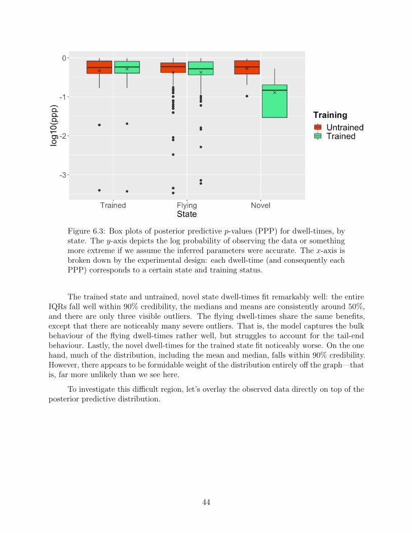
Figure 6.3: Box plots of posterior predictive p-values (PPP) for dwell-times, bystate. The y-axis depicts the log probability of observing the data or somethingmore extreme if we assume the inferred parameters were accurate. The x-axis isbroken down by the experimental design: each dwell-time (and consequently eachPPP) corresponds to a certain state and training status.

The trained state and untrained, novel state dwell-times fit remarkably well: the entireIQRs fall well within 90% credibility, the medians and means are consistently around 50%,and there are only three visible outliers. The flying dwell-times share the same benefits,except that there are noticeably many severe outliers. That is, the model captures the bulkbehaviour of the flying dwell-times rather well, but struggles to account for the tail-endbehaviour. Lastly, the novel dwell-times for the trained state fit noticeably worse. On the onehand, much of the distribution, including the mean and median, falls within 90% credibility.However, there appears to be formidable weight of the distribution entirely off the graph—thatis, far more unlikely than we see here.

To investigate this difficult region, let’s overlay the observed data directly on top of theposterior predictive distribution.

44

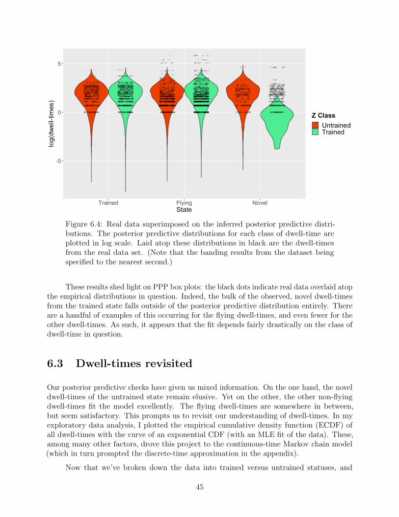
Figure 6.4: Real data superimposed on the inferred posterior predictive distri-butions. The posterior predictive distributions for each class of dwell-time areplotted in log scale. Laid atop these distributions in black are the dwell-timesfrom the real data set. (Note that the banding results from the dataset beingspecified to the nearest second.)

These results shed light on PPP box plots: the black dots indicate real data overlaid atopthe empirical distributions in question. Indeed, the bulk of the observed, novel dwell-timesfrom the trained state falls outside of the posterior predictive distribution entirely. Thereare a handful of examples of this occurring for the flying dwell-times, and even fewer for theother dwell-times. As such, it appears that the fit depends fairly drastically on the class ofdwell-time in question.

6.3 Dwell-times revisited

Our posterior predictive checks have given us mixed information. On the one hand, the noveldwell-times of the untrained state remain elusive. Yet on the other, the other non-flyingdwell-times fit the model excellently. The flying dwell-times are somewhere in between,but seem satisfactory. This prompts us to revisit our understanding of dwell-times. In myexploratory data analysis, I plotted the empirical cumulative density function (ECDF) ofall dwell-times with the curve of an exponential CDF (with an MLE fit of the data). These,among many other factors, drove this project to the continuous-time Markov chain model(which in turn prompted the discrete-time approximation in the appendix).

Now that we’ve broken down the data into trained versus untrained statuses, and

45

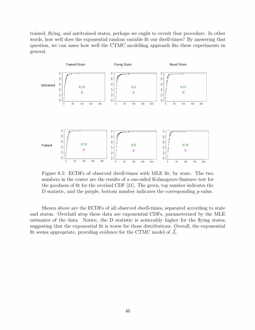
trained, flying, and antitrained states, perhaps we ought to revisit that procedure. In otherwords, how well does the exponential random variable fit our dwell-times? By answering thatquestion, we can asses how well the CTMC modelling approach fits these experiments ingeneral.

Figure 6.5: ECDFs of observed dwell-times with MLE fit, by state. The twonumbers in the center are the results of a one-sided Kolmogorov-Smirnov test forthe goodness of fit for the overlaid CDF [21]. The green, top number indicates theD statistic, and the purple, bottom number indicates the corresponding p-value.

Shown above are the ECDFs of all observed dwell-times, separated according to stateand status. Overlaid atop these data are exponential CDFs, parameterized by the MLEestimates of the data. Notice, the D statistic is noticeably higher for the flying states,suggesting that the exponential fit is worse for those distributions. Overall, the exponentialfit seems appropriate, providing evidence for the CTMC model of ~Ji.

46

Chapter 7

Future Directions

We’ve seen the continuous-time Markov chain modeling approach produce results that matchand expand upon our understanding of the biology. As outlined in the appendix, the discrete-time model excels at rapid inference with very weak prior information, resulting in reasonabletraining classification and regression inference. The discrete-time Markov chain model ofthe data thus proves sufficient to a first approximation at making our desired inference,including an approximation of the dwell-time distributions. The continuous-time model,while computationally more intensive, models time notably better than the DTM. We seeexcellent fit for the floral dwell-times, with the exception of those pertaining to the novelstate and untrained status.

The continuous-time algorithm requires more prior information than its discrete-timecounterpart. The CTM is more fragile: without help in parsing which rate matrices corre-sponded to which training states, it sticks to local modes wherein all bees are classified inthe same state. To avoid both this issue and the label-switching problem, we instituted amore sophisticated, empirical prior search. We translated our ideas on how trained versusuntrained bees behave into rate matrices, which helped the algorithm converge consistentlyand faster. These rate matrices fit the floral dwell-times even better, and modelled timemore honestly. However, the issues of the DTM persisted, as the flying and novel-traineddwell-times resulted in suboptimal posterior predictive p-values.

I originally assumed that I would be following a progression from discrete-time, tocontinuous-time, to then loosening the exponential dwell-time requirement. This last featurewould require a semi-Markov process, which in addition to being more difficult to model(not to mention the memorylessness property would be lost), actually seems unnecessary.Recall that the exponential dwell-time fit is far from the greatest issue: in addition to beingmostly consistent across the floral dwell-times from a goodness-of-fit perspective, the posteriorpredictive p-values are quite promising. Indeed, the weakest part of the exponential fit—theflying dwell-times—is also the least biologically pertinent part of the model.

In general, the CTM appeared to be a more specific, consistent, and confident versionof the DTM. However, this resulted in more conservative estimates, where some bees thatare likely more trained than untrained were classified as entirely untrained. I am confidentthis stems from the prior being too rigid. The prior I’ve outlined represents a first attempt; Ihave yet to fine-tune how much weight to give the initial rate matrices, and how much leewayto give the algorithm to find a compromise between the bees that are unequivocally trainedand those that aren’t quite there. We can likely accomplish this with less strict rate matrices,rather than replacing the ~Z dichotomy with a spectrum. This process of prior refinement isthe most immediate and attainable next step.

47

While in my exploratory data analysis I’ve repeatedly found evidence suggesting thatcolony doesn’t require an explicit random effect, we have begun to glimpse that training mightactually look different depending on training color. The DTM argued that blue increasestraining over 5 to 1, and the CTM doubled that figure. A more honest phenomenon is likelythat training simply looks different depending on color. Perhaps white training is simply lesssevere: we ought to model this at the ~λ level, rather than the ~Z level. As a more exciting nextstep, I will begin to build out a regression scheme on the rate matrix parameters themselves,allowing the training treatments to explicitly affect the definition of training (in additionto the latent probability of training that we currently model). I will likely use HamiltonianMonte Carlo to accomplish this [22].

The work thus far has not only served to offer reasonable first results, but validatedthe usefulness of modeling these types of experiments from a Bayesian context. In the nearfuture I hope to offer the insect ethology community the toolkit to holistically, thoroughly,and efficiently analyze secondary metabolite training experiments.

48

Appendices

49

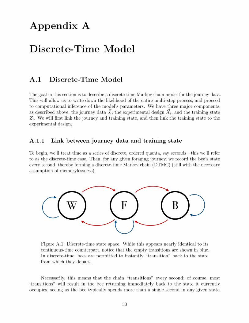
Appendix A

Discrete-Time Model

A.1 Discrete-Time Model

The goal in this section is to describe a discrete-time Markov chain model for the journey data.This will allow us to write down the likelihood of the entire multi-step process, and proceedto computational inference of the model’s parameters. We have three major components,as described above, the journey data ~Ji, the experimental design ~Xi, and the training stateZi. We will first link the journey and training state, and then link the training state to theexperimental design.

A.1.1 Link between journey data and training state

To begin, we’ll treat time as a series of discrete, ordered quanta, say seconds—this we’ll referto as the discrete-time case. Then, for any given foraging journey, we record the bee’s stateevery second, thereby forming a discrete-time Markov chain (DTMC) (still with the necessaryassumption of memorylessness).

Figure A.1: Discrete-time state space. While this appears nearly identical to itscontinuous-time counterpart, notice that the empty transitions are shown in blue.In discrete-time, bees are permitted to instantly “transition” back to the statefrom which they depart.

Necessarily, this means that the chain “transitions” every second; of course, most“transitions” will result in the bee returning immediately back to the state it currentlyoccupies, seeing as the bee typically spends more than a single second in any given state.

50

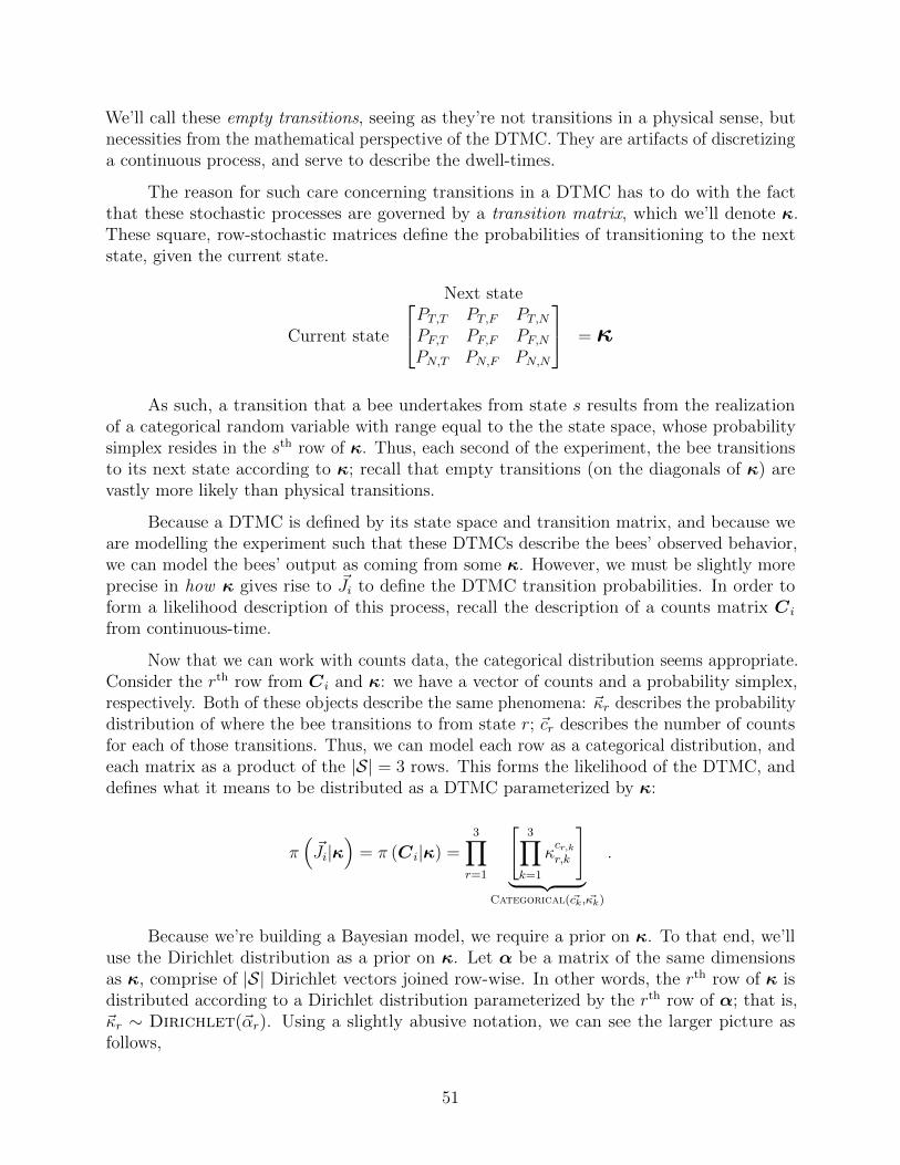
We’ll call these empty transitions, seeing as they’re not transitions in a physical sense, butnecessities from the mathematical perspective of the DTMC. They are artifacts of discretizinga continuous process, and serve to describe the dwell-times.

The reason for such care concerning transitions in a DTMC has to do with the factthat these stochastic processes are governed by a transition matrix, which we’ll denote κ.These square, row-stochastic matrices define the probabilities of transitioning to the nextstate, given the current state.

Next state

Current state

PT,T PT,F PT,NPF,T PF,F PF,NPN,T PN,F PN,N

=κ

As such, a transition that a bee undertakes from state s results from the realizationof a categorical random variable with range equal to the the state space, whose probabilitysimplex resides in the sth row of κ. Thus, each second of the experiment, the bee transitionsto its next state according to κ; recall that empty transitions (on the diagonals of κ) arevastly more likely than physical transitions.

Because a DTMC is defined by its state space and transition matrix, and because weare modelling the experiment such that these DTMCs describe the bees’ observed behavior,we can model the bees’ output as coming from some κ. However, we must be slightly moreprecise in how κ gives rise to ~Ji to define the DTMC transition probabilities. In order toform a likelihood description of this process, recall the description of a counts matrix Ci

from continuous-time.

Now that we can work with counts data, the categorical distribution seems appropriate.Consider the rth row from Ci and κ: we have a vector of counts and a probability simplex,respectively. Both of these objects describe the same phenomena: ~κr describes the probabilitydistribution of where the bee transitions to from state r; ~cr describes the number of countsfor each of those transitions. Thus, we can model each row as a categorical distribution, andeach matrix as a product of the |S| = 3 rows. This forms the likelihood of the DTMC, anddefines what it means to be distributed as a DTMC parameterized by κ:

π(~Ji|κ

)= π (Ci|κ) =

3∏r=1

[3∏

k=1

κcr,kr,k

]︸ ︷︷ ︸

Categorical( ~ck, ~κk)

.

Because we’re building a Bayesian model, we require a prior on κ. To that end, we’lluse the Dirichlet distribution as a prior on κ. Let α be a matrix of the same dimensionsas κ, comprise of |S| Dirichlet vectors joined row-wise. In other words, the rth row of κ isdistributed according to a Dirichlet distribution parameterized by the rth row of α; that is,~κr ∼ Dirichlet(~αr). Using a slightly abusive notation, we can see the larger picture asfollows,

51

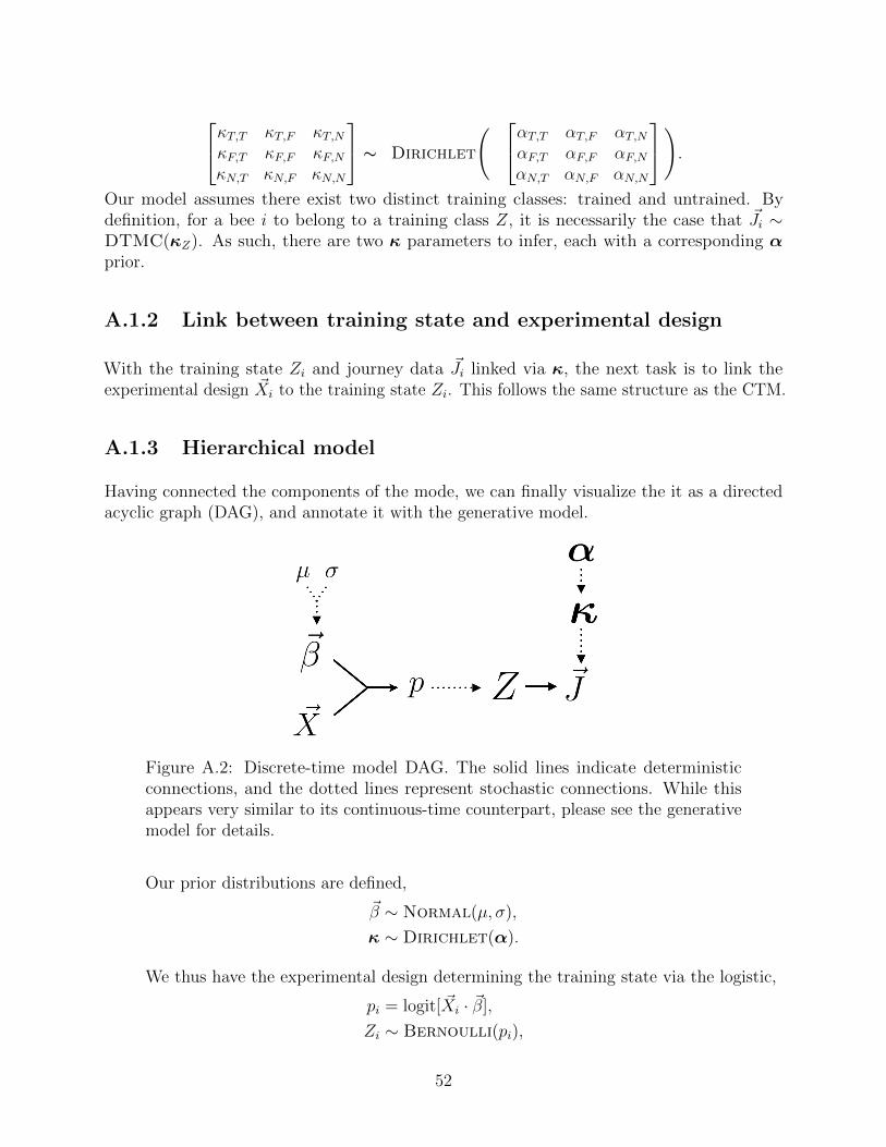
κT,T κT,F κT,NκF,T κF,F κF,NκN,T κN,F κN,N

∼ Dirichlet

( αT,T αT,F αT,NαF,T αF,F αF,NαN,T αN,F αN,N

).Our model assumes there exist two distinct training classes: trained and untrained. Bydefinition, for a bee i to belong to a training class Z, it is necessarily the case that ~Ji ∼DTMC(κZ). As such, there are two κ parameters to infer, each with a corresponding αprior.

A.1.2 Link between training state and experimental design

With the training state Zi and journey data ~Ji linked via κ, the next task is to link theexperimental design ~Xi to the training state Zi. This follows the same structure as the CTM.

A.1.3 Hierarchical model

Having connected the components of the mode, we can finally visualize the it as a directedacyclic graph (DAG), and annotate it with the generative model.

Figure A.2: Discrete-time model DAG. The solid lines indicate deterministicconnections, and the dotted lines represent stochastic connections. While thisappears very similar to its continuous-time counterpart, please see the generativemodel for details.

Our prior distributions are defined,

~β ∼ Normal(µ, σ),

κ ∼ Dirichlet(α).

We thus have the experimental design determining the training state via the logistic,

pi = logit[ ~Xi · ~β],

Zi ∼ Bernoulli(pi),

52

and the training state determining the journey data,

~Ji|κZi∼ DTMC(κZi

),

π( ~Ji|κZi) =

3∏r=1

[3∏

k=1

κcr,kr,k

].

A.2 Discrete-Time Algorithm

As outlined before, the DTM algorithm alternates between updating the transition matrices κ,the regression coefficients ~β, and the training states ~Z. Once again, time is the differentiatingfeature; it will affect not just the Markov chain likelihood, but the training state posteriors(and ultimately the regression coefficients). The following explanation of each type of movewill outline how we sample from each conditional posterior.

A.2.1 Move 1: Gibbs sampler for updating the transition matrices

For this process, we know that the transition matrices and their Dirichlet parameters areconditionally independent of the regression parameters, given the training states. Thus, wecan consider only the Dirichlet and transition matrices with the training states. Recall thediscussion from the previous section. The ith row of κ (the transition matrix) is distributedas a Dirichlet of the form Diric(κi,1, κi,2, κi,3|αi,1, αi,2, αi,3), or more succinctly Diric(~κi|~αi),for i ∈ S.

To develop this idea, consider the probability density of the Dirichlet distribution,

π(κi, . . . , κk|α1, . . . , αk) =1

B(~α)

K∏i=1

καi−1i ,

where∑k

i=1 κi = 1, and κi ≥ 0 for all i ∈ {1, . . . , K}; and the normalizing constant in termsof the multivariate beta function is

B(~α) =

∏Ki=1 Γ(αi)

Γ(∑K

i=1 αi).

We can use this function to demonstrate that the Dirichlet distribution is a conjugate priorof the categorical distribution (shown in the appendix)1. Recall that conjugacy refers toa particular pair of prior and likelihood distributions interacting such that the posteriordistribution is of the same form as the prior.

As a typical Gibbs sampler, this type of move is effectively sampling from the conditionaldistribution of the three ~κ’s, conditioned upon a given set of training outcomes ~Z. Suppose

1Note that the appendix demonstrates multinomial-Dirichlet conjugacy, which is a slightly more generalform of what our model requires.

53

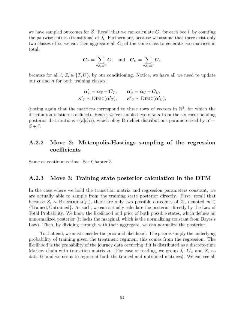
we have sampled outcomes for ~Z. Recall that we can calculate Ci for each bee i, by countingthe pairwise entries (transitions) of ~Ji. Furthermore, because we assume that there exist onlytwo classes of α, we can then aggregate all Ci of the same class to generate two matrices intotal:

CT =∑∀Zi=T

Ci and CU =∑∀Zi=U

Ci,

because for all i, Zi ∈ {T, U}, by our conditioning. Notice, we have all we need to updateour α and κ for both training classes:

α′T = αT +CT , α′U = αU +CU ,

κ′T ∼ Diric(α′

T ), κ′U ∼ Diric(α′

U),

(noting again that the matrices correspond to three rows of vectors in R3, for which thedistribution relation is defined). Hence, we’ve sampled two new κ from the six correspondingposterior distributions π(~κ|~c, ~α), which obey Dirichlet distributions parameterized by ~α′ =~α + ~c.

A.2.2 Move 2: Metropolis-Hastings sampling of the regressioncoefficients

Same as continuous-time. See Chapter 3.

A.2.3 Move 3: Training state posterior calculation in the DTM

In the case where we hold the transition matrix and regression parameters constant, weare actually able to sample from the training state posterior directly. First, recall thatbecause Zi ∼ Bernoulli(pi), there are only two possible outcomes of Zi, denoted m ∈{Trained,Untrained}. As such, we can actually calculate the posterior directly by the Law ofTotal Probability. We know the likelihood and prior of both possible states, which defines anunnormalized posterior (it lacks the marginal, which is the normalizing constant from Bayes’sLaw). Then, by dividing through with their aggregate, we can normalize the posterior.

To that end, we must consider the prior and likelihood. The prior is simply the underlyingprobability of training given the treatment regimen; this comes from the regression. Thelikelihood is the probability of the journey data occurring if it is distributed as a discrete-timeMarkov chain with transition matrix κ. (For ease of reading, we group ~Ji, Ci, and ~Xi asdata D; and we use κ to represent both the trained and untrained matrices). We can see all

54

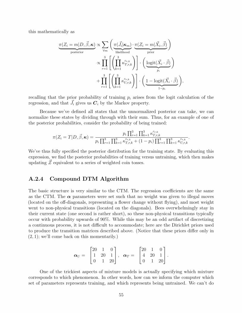
this mathematically as

π(Zi = m|D, ~β,κ)︸ ︷︷ ︸posterior

∝∑∀m

(π( ~Ji|κm)︸ ︷︷ ︸

likelihood

·π(Zi = m| ~Xi, ~β)︸ ︷︷ ︸prior

)

∝3∏r=1

[(3∏

k=1

κcr,kT,r,k

)]·(

logit( ~Xi · ~β)︸ ︷︷ ︸pi

)

+3∏r=1

[(3∏

k=1

κcr,kU,r,k

)]·(

1− logit( ~Xi · ~β)︸ ︷︷ ︸1−pi

),

recalling that the prior probability of training pi arises from the logit calculation of theregression, and that ~Ji gives us Ci by the Markov property.

Because we’ve defined all states that the unnormalized posterior can take, we cannormalize these states by dividing through with their sum. Thus, for an example of one ofthe posterior probabilities, consider the probability of being trained:

π(Zi = T |D, ~β,κ) =pi∏3

r=1

∏3k=1 κ

cr,kT,r,k

pi∏3

r=1

∏3k=1 κ

cr,kT,r,k + (1− pi)

∏3r=1

∏3k=1 κ

cr,kU,r,k

.

We’ve thus fully specified the posterior distribution for the training state. By evaluating thisexpression, we find the posterior probabilities of training versus untraining, which then makesupdating ~Z equivalent to a series of weighted coin tosses.

A.2.4 Compound DTM Algorithm

The basic structure is very similar to the CTM. The regression coefficients are the sameas the CTM. The α parameters were set such that no weight was given to illegal moves(located on the off-diagonals, representing a flower change without flying), and most weightwent to non-physical transitions (located on the diagonals). Bees overwhelmingly stay intheir current state (one second is rather short), so these non-physical transitions typicallyoccur with probability upwards of 90%. While this may be an odd artifact of discretizinga continuous process, it is not difficult to accommodate; here are the Dirichlet priors usedto produce the transition matrices described above. (Notice that these priors differ only in(2, 1); we’ll come back on this momentarily.)

αU =

20 1 01 20 10 1 20

, αT =

20 1 04 20 10 1 20

.One of the trickiest aspects of mixture models is actually specifying which mixture

corresponds to which phenomenon. In other words, how can we inform the computer whichset of parameters represents training, and which represents being untrained. We can’t do

55

this after the fact—the regression coefficients change depending on whether the algorithmassigns the proper κ parameters or switches them (each of these labeling schemes beingequally likely). To that end, we employ a step in the algorithm that we call the unmixingstep. After the first round of tempering the κ parameters with the training states, we inspectthe training states of a group of bees whose training states are obvious from inspecting thedata. These are called core bees, and only ever visit their trained flower. Overwhelmingly,these bees are all either classified as ones or zeros. In the case that they are zero, we switchthem to one, and reassign which κ and α parameters go to which training state. This isknown as the label switching problem [16].

Recall the transformation of the state space in Chapter 4. When we discuss (2, 1) ofa transition matrix, we know that, independent of the training color, we are investigatingthe probability of going from flying to the trained state. Thus, when our prior assigns moreweight to that entry, it reflects our prior belief that a trained bee will choose a trained statemore frequently than a novel state. However, should the label switching problem occur(which still happens, but less frequently), we switch the priors as well, because they make theargument that trained and untrained bees behave differently a priori of the data.

A.3 Simulation Studies

Note that this these studies are very similar to their continuous-time counterparts. Notethat a novel performance metric will be employed to assess the distance in κ. Because eachrow of κ represents a probability distribution, we calculate the row-wise Jenson-ShannonDivergence (JSD) [23] of each estimated κ from the underlying κ (as such, the calculatedvalue reflects the sum of six different JSD values). Once again, identical matrices will haveJSD equal to zero. The following demonstrates convergence for the DTM (again, parameterslocated in the appendix for Chapter 5).

56

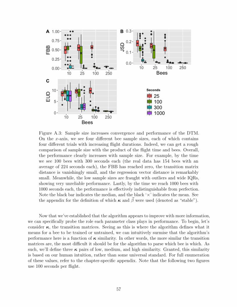
Figure A.3: Sample size increases convergence and performance of the DTM.On the x-axis, we see four different bee sample sizes, each of which containsfour different trials with increasing flight durations. Indeed, we can get a roughcomparison of sample size with the product of the flight time and bees. Overall,the performance clearly increases with sample size. For example, by the timewe see 100 bees with 300 seconds each (the real data has 154 bees with anaverage of 224 seconds each), the FBB has reached zero, the transition matrixdistance is vanishingly small, and the regression vector distance is remarkablysmall. Meanwhile, the low sample sizes are fraught with outliers and wide IQRs,showing very unreliable performance. Lastly, by the time we reach 1000 bees with1000 seconds each, the performance is effectively indistinguishable from perfection.Note the black bar indicates the median, and the black ‘×’ indicates the mean. Seethe appendix for the definition of which κ and ~β were used (denoted as “stable”).

Now that we’ve established that the algorithm appears to improve with more information,we can specifically probe the role each parameter class plays in performance. To begin, let’sconsider κ, the transition matrices. Seeing as this is where the algorithm defines what itmeans for a bee to be trained or untrained, we can intuitively surmise that the algorithm’sperformance here is a function of κ similarity. In other words, the more similar the transitionmatrices are, the most difficult it should be for the algorithm to parse which bee is which. Assuch, we’ll define three κ pairs of low, medium, and high similarity. Granted, this similarityis based on our human intuition, rather than some universal standard. For full enumerationof these values, refer to the chapter-specific appendix. Note that the following two figuresuse 100 seconds per flight.

57

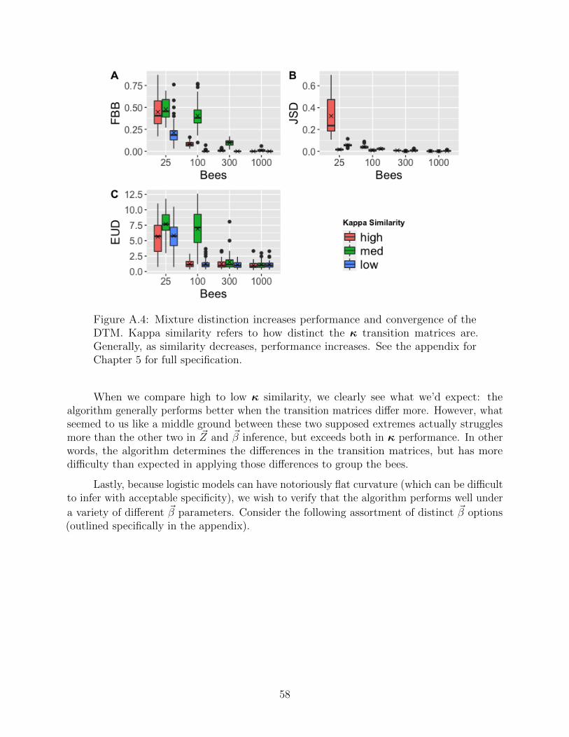
Figure A.4: Mixture distinction increases performance and convergence of theDTM. Kappa similarity refers to how distinct the κ transition matrices are.Generally, as similarity decreases, performance increases. See the appendix forChapter 5 for full specification.

When we compare high to low κ similarity, we clearly see what we’d expect: thealgorithm generally performs better when the transition matrices differ more. However, whatseemed to us like a middle ground between these two supposed extremes actually strugglesmore than the other two in ~Z and ~β inference, but exceeds both in κ performance. In otherwords, the algorithm determines the differences in the transition matrices, but has moredifficulty than expected in applying those differences to group the bees.

Lastly, because logistic models can have notoriously flat curvature (which can be difficultto infer with acceptable specificity), we wish to verify that the algorithm performs well under

a variety of different ~β parameters. Consider the following assortment of distinct ~β options(outlined specifically in the appendix).

58

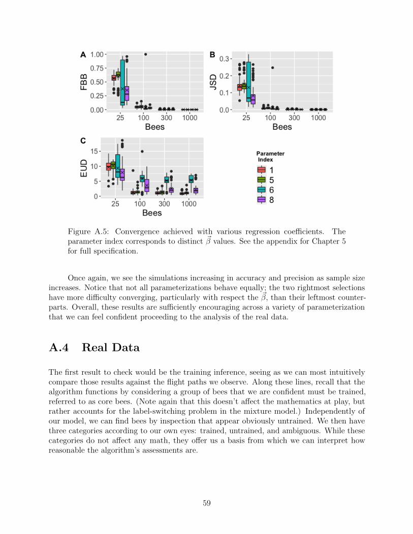
Figure A.5: Convergence achieved with various regression coefficients. Theparameter index corresponds to distinct ~β values. See the appendix for Chapter 5for full specification.

Once again, we see the simulations increasing in accuracy and precision as sample sizeincreases. Notice that not all parameterizations behave equally; the two rightmost selectionshave more difficulty converging, particularly with respect the ~β, than their leftmost counter-parts. Overall, these results are sufficiently encouraging across a variety of parameterizationthat we can feel confident proceeding to the analysis of the real data.

A.4 Real Data

The first result to check would be the training inference, seeing as we can most intuitivelycompare those results against the flight paths we observe. Along these lines, recall that thealgorithm functions by considering a group of bees that we are confident must be trained,referred to as core bees. (Note again that this doesn’t affect the mathematics at play, butrather accounts for the label-switching problem in the mixture model.) Independently ofour model, we can find bees by inspection that appear obviously untrained. We then havethree categories according to our own eyes: trained, untrained, and ambiguous. While thesecategories do not affect any math, they offer us a basis from which we can interpret howreasonable the algorithm’s assessments are.

59

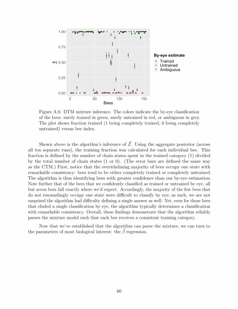
Figure A.6: DTM mixture inference. The colors indicate the by-eye classificationof the bees: surely trained in green, surely untrained in red, or ambiguous in grey.The plot shows fraction trained (1 being completely trained, 0 being completelyuntrained) versus bee index.

Shown above is the algorthm’s inference of ~Z. Using the aggregate posterior (acrossall ten separate runs), the training fraction was calculated for each individual bee. Thisfraction is defined by the number of chain states spent in the trained category (1) dividedby the total number of chain states (1 or 0). (The error bars are defined the same wayas the CTM.) First, notice that the overwhelming majority of bees occupy one state withremarkable consistency: bees tend to be either completely trained or completely untrained.The algorithm is thus identifying bees with greater confidence than our by-eye estimation.Note further that of the bees that we confidently classified as trained or untrained by eye, allbut seven bees fall exactly where we’d expect. Accordingly, the majority of the few bees thatdo not resoundingly occupy one state were difficult to classify by eye; as such, we are notsurprised the algorithm had difficulty defining a single answer as well. Yet, even for those beesthat eluded a single classification by eye, the algorithm typically determines a classificationwith remarkable consistency. Overall, these findings demonstrate that the algorithm reliablyparses the mixture model such that each bee receives a consistent training category.

Now that we’ve established that the algorithm can parse the mixture, we can turn tothe parameters of most biological interest: the ~β regression.

60

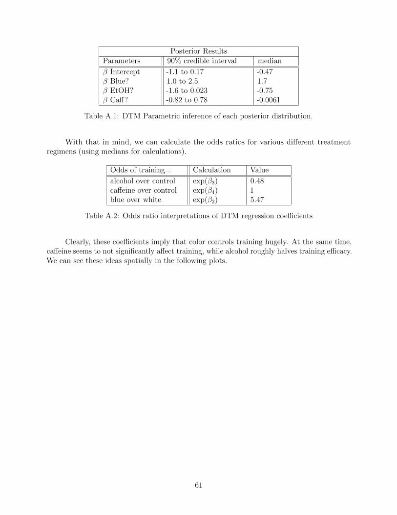
Posterior ResultsParameters 90% credible interval median

β Intercept -1.1 to 0.17 -0.47β Blue? 1.0 to 2.5 1.7β EtOH? -1.6 to 0.023 -0.75β Caff? -0.82 to 0.78 -0.0061

Table A.1: DTM Parametric inference of each posterior distribution.

With that in mind, we can calculate the odds ratios for various different treatmentregimens (using medians for calculations).

Odds of training... Calculation Value

alcohol over control exp(β3) 0.48caffeine over control exp(β4) 1blue over white exp(β2) 5.47

Table A.2: Odds ratio interpretations of DTM regression coefficients

Clearly, these coefficients imply that color controls training hugely. At the same time,caffeine seems to not significantly affect training, while alcohol roughly halves training efficacy.We can see these ideas spatially in the following plots.

61

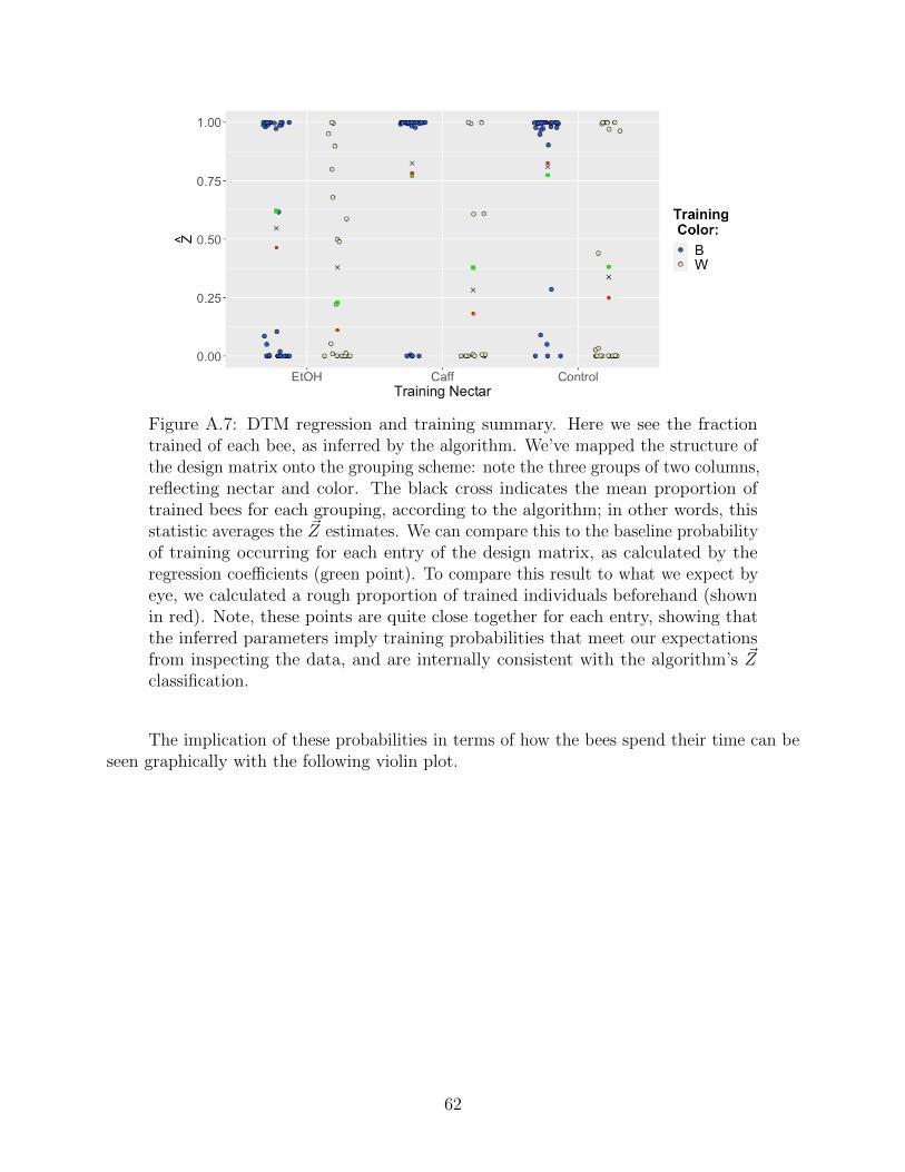
Figure A.7: DTM regression and training summary. Here we see the fractiontrained of each bee, as inferred by the algorithm. We’ve mapped the structure ofthe design matrix onto the grouping scheme: note the three groups of two columns,reflecting nectar and color. The black cross indicates the mean proportion oftrained bees for each grouping, according to the algorithm; in other words, thisstatistic averages the ~Z estimates. We can compare this to the baseline probabilityof training occurring for each entry of the design matrix, as calculated by theregression coefficients (green point). To compare this result to what we expect byeye, we calculated a rough proportion of trained individuals beforehand (shownin red). Note, these points are quite close together for each entry, showing thatthe inferred parameters imply training probabilities that meet our expectationsfrom inspecting the data, and are internally consistent with the algorithm’s ~Zclassification.

The implication of these probabilities in terms of how the bees spend their time can beseen graphically with the following violin plot.

62

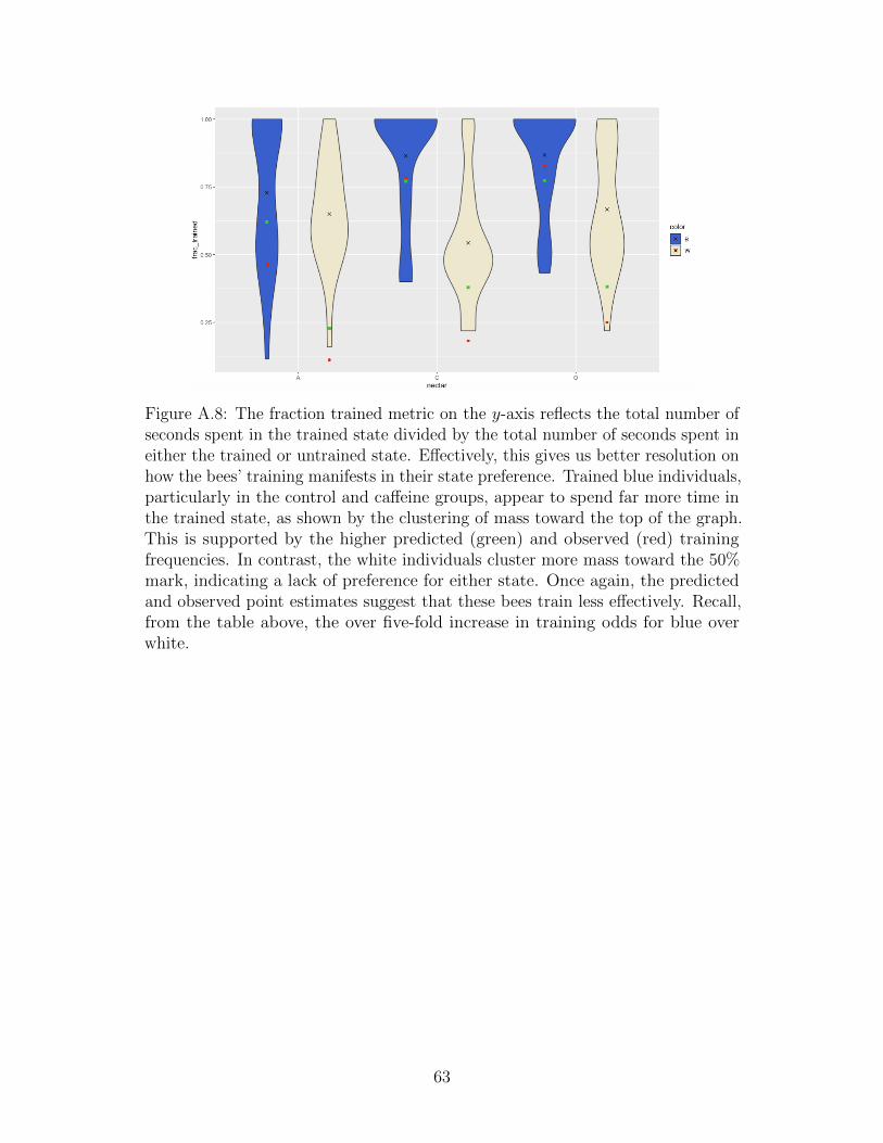
Figure A.8: The fraction trained metric on the y-axis reflects the total number ofseconds spent in the trained state divided by the total number of seconds spent ineither the trained or untrained state. Effectively, this gives us better resolution onhow the bees’ training manifests in their state preference. Trained blue individuals,particularly in the control and caffeine groups, appear to spend far more time inthe trained state, as shown by the clustering of mass toward the top of the graph.This is supported by the higher predicted (green) and observed (red) trainingfrequencies. In contrast, the white individuals cluster more mass toward the 50%mark, indicating a lack of preference for either state. Once again, the predictedand observed point estimates suggest that these bees train less effectively. Recall,from the table above, the over five-fold increase in training odds for blue overwhite.

63

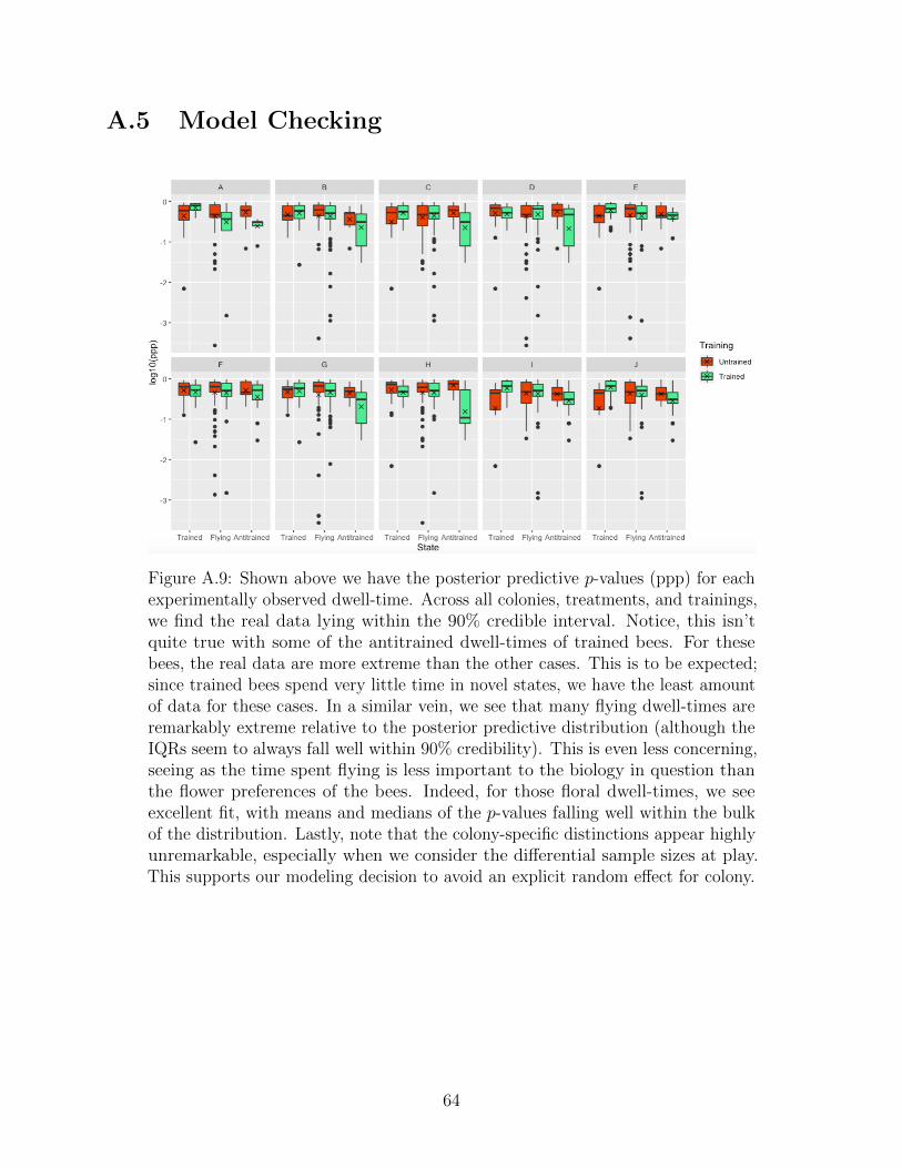
A.5 Model Checking

Figure A.9: Shown above we have the posterior predictive p-values (ppp) for eachexperimentally observed dwell-time. Across all colonies, treatments, and trainings,we find the real data lying within the 90% credible interval. Notice, this isn’tquite true with some of the antitrained dwell-times of trained bees. For thesebees, the real data are more extreme than the other cases. This is to be expected;since trained bees spend very little time in novel states, we have the least amountof data for these cases. In a similar vein, we see that many flying dwell-times areremarkably extreme relative to the posterior predictive distribution (although theIQRs seem to always fall well within 90% credibility). This is even less concerning,seeing as the time spent flying is less important to the biology in question thanthe flower preferences of the bees. Indeed, for those floral dwell-times, we seeexcellent fit, with means and medians of the p-values falling well within the bulkof the distribution. Lastly, note that the colony-specific distinctions appear highlyunremarkable, especially when we consider the differential sample sizes at play.This supports our modeling decision to avoid an explicit random effect for colony.

64

Appendix B

Chapter-Specific Appendices

65

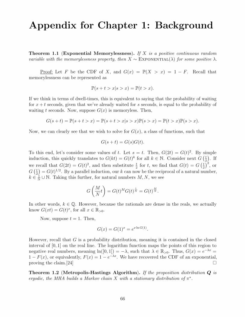
Appendix for Chapter 1: Background

Theorem 1.1 (Exponential Memorylessness). If X is a positive continuous randomvariable with the memorylessness property, then X ∼ Exponential(λ) for some positive λ.

Proof: Let F be the CDF of X, and G(x) = P(X > x) = 1 − F . Recall thatmemorylessness can be represented as

P(s+ t > x|s > x) = P(t > x).

If we think in terms of dwell-times, this is equivalent to saying that the probability of waitingfor x+ t seconds, given that we’ve already waited for s seconds, is equal to the probability ofwaiting t seconds. Now, suppose G(x) is memoryless. Then,

G(s+ t) = P(s+ t > x) = P(s+ t > x|s > x)P(s > x) = P(t > x)P(s > x).

Now, we can clearly see that we wish to solve for G(x), a class of functions, such that

G(s+ t) = G(s)G(t).

To this end, let’s consider some values of t. Let s = t. Then, G(2t) = G(t)2. By simpleinduction, this quickly translates to G(kt) = G(t)k for all k ∈ N. Consider next G

(t2

). If

we recall that G(2t) = G(t)2, and then substitute t2

for t, we find that G(t) = G(t2

)2, or

G(t2

)= G(t)1/2. By a parallel induction, our k can now be the reciprocal of a natural number,

k ∈ 1N ∪ N. Taking this further, for natural numbers M,N , we see

G

(M

Nt

)= G(t)MG(t)

1N = G(t)

MN .

In other words, k ∈ Q. However, because the rationals are dense in the reals, we actuallyknow G(xt) = G(t)x, for all x ∈ R>0.

Now, suppose t = 1. Then,

G(x) = G(1)x = ex lnG(1).

However, recall that G is a probability distribution, meaning it is contained in the closedinterval of [0, 1] on the real line. The logarithm function maps the points of this region tonegative real numbers, meaning ln([0, 1]) = −λ, such that λ ∈ R>0. Thus, G(x) = e−λx =1− F (x), or equivalently, F (x) = 1− e−λx. We have recovered the CDF of an exponential,proving the claim.[24]

Theorem 1.2 (Metropolis-Hastings Algorithm). If the proposition distribution Q isergodic, the MHA builds a Markov chain X with a stationary distribution of π∗.

66

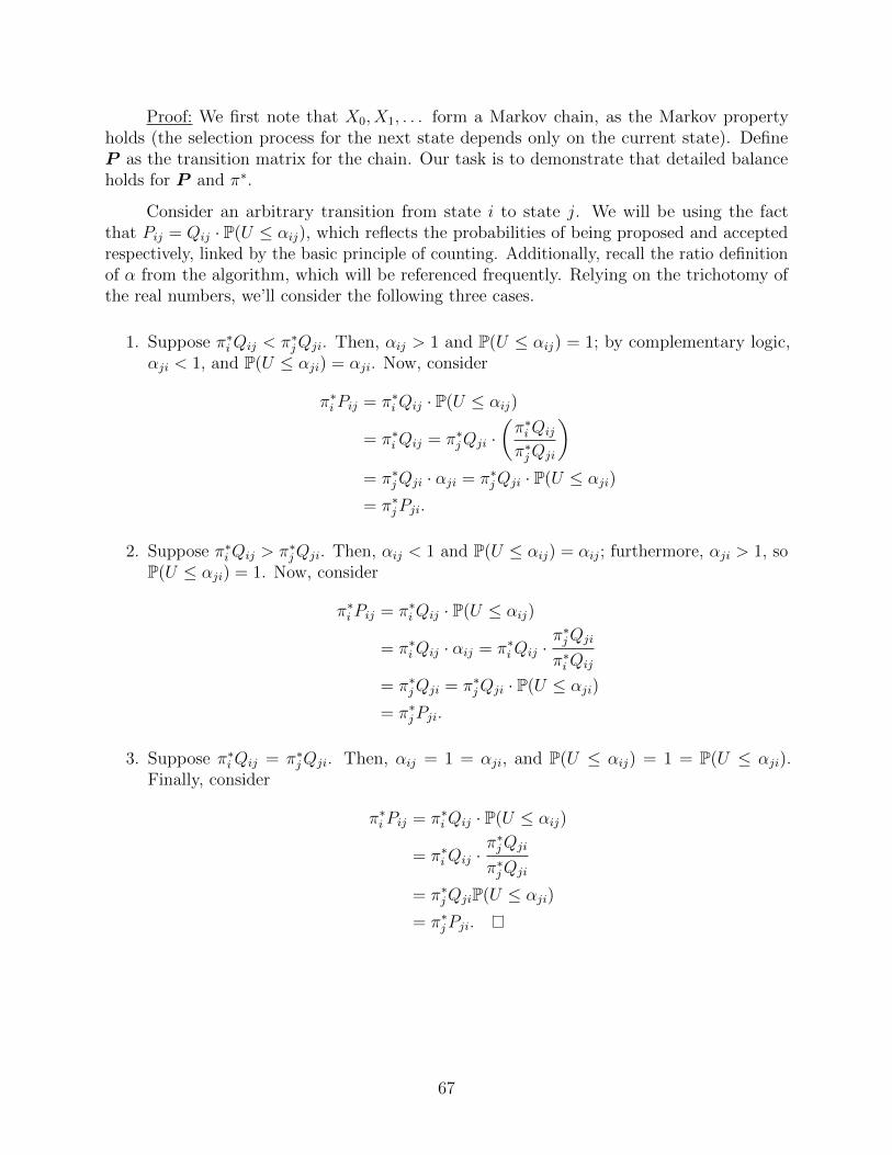
Proof: We first note that X0, X1, . . . form a Markov chain, as the Markov propertyholds (the selection process for the next state depends only on the current state). DefineP as the transition matrix for the chain. Our task is to demonstrate that detailed balanceholds for P and π∗.

Consider an arbitrary transition from state i to state j. We will be using the factthat Pij = Qij · P(U ≤ αij), which reflects the probabilities of being proposed and acceptedrespectively, linked by the basic principle of counting. Additionally, recall the ratio definitionof α from the algorithm, which will be referenced frequently. Relying on the trichotomy ofthe real numbers, we’ll consider the following three cases.

1. Suppose π∗iQij < π∗jQji. Then, αij > 1 and P(U ≤ αij) = 1; by complementary logic,αji < 1, and P(U ≤ αji) = αji. Now, consider

π∗i Pij = π∗iQij · P(U ≤ αij)

= π∗iQij = π∗jQji ·(π∗iQij

π∗jQji

)= π∗jQji · αji = π∗jQji · P(U ≤ αji)

= π∗jPji.

2. Suppose π∗iQij > π∗jQji. Then, αij < 1 and P(U ≤ αij) = αij; furthermore, αji > 1, soP(U ≤ αji) = 1. Now, consider

π∗i Pij = π∗iQij · P(U ≤ αij)

= π∗iQij · αij = π∗iQij ·π∗jQji

π∗iQij

= π∗jQji = π∗jQji · P(U ≤ αji)

= π∗jPji.

3. Suppose π∗iQij = π∗jQji. Then, αij = 1 = αji, and P(U ≤ αij) = 1 = P(U ≤ αji).Finally, consider

π∗i Pij = π∗iQij · P(U ≤ αij)

= π∗iQij ·π∗jQji

π∗jQji

= π∗jQjiP(U ≤ αji)

= π∗jPji.

67

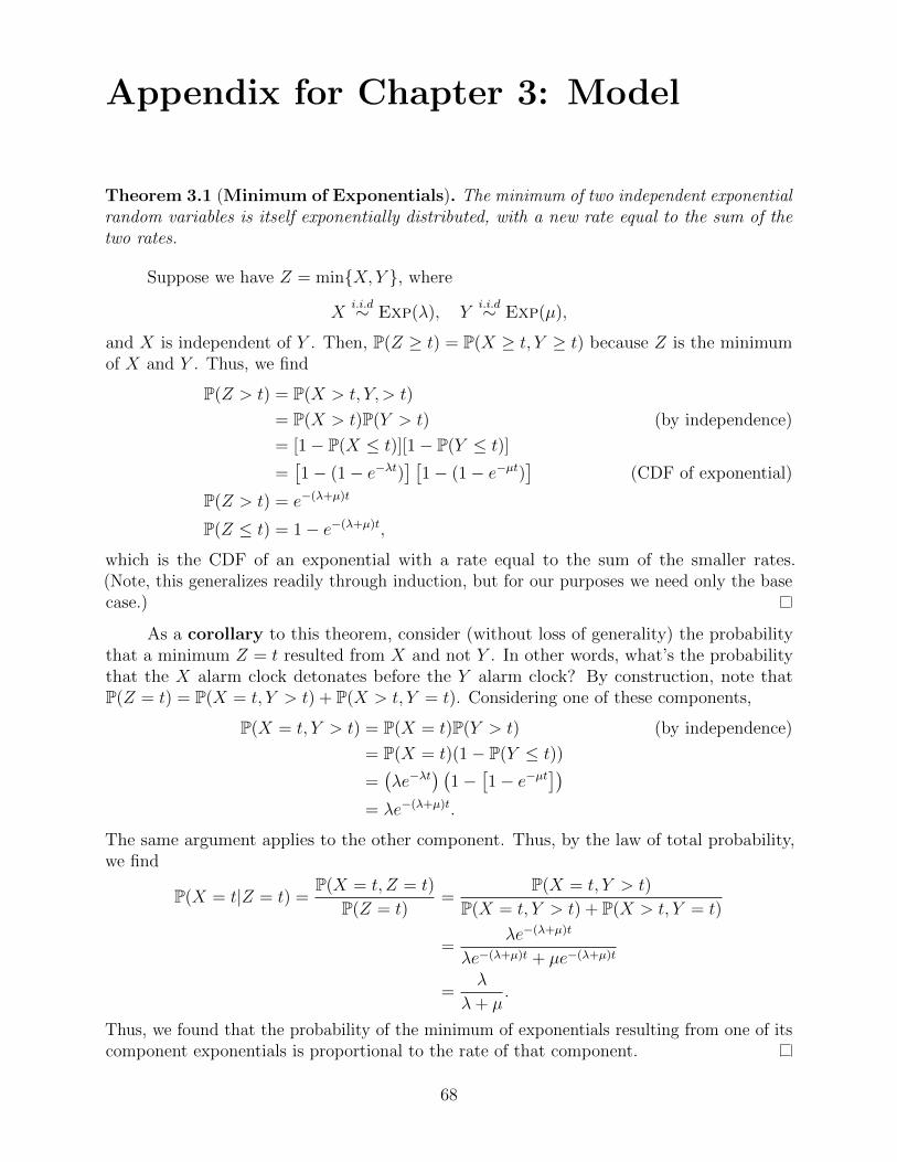
Appendix for Chapter 3: Model

Theorem 3.1 (Minimum of Exponentials). The minimum of two independent exponentialrandom variables is itself exponentially distributed, with a new rate equal to the sum of thetwo rates.

Suppose we have Z = min{X, Y }, where

Xi.i.d∼ Exp(λ), Y

i.i.d∼ Exp(µ),

and X is independent of Y . Then, P(Z ≥ t) = P(X ≥ t, Y ≥ t) because Z is the minimumof X and Y . Thus, we find

P(Z > t) = P(X > t, Y,> t)

= P(X > t)P(Y > t) (by independence)

= [1− P(X ≤ t)][1− P(Y ≤ t)]

=[1− (1− e−λt)

] [1− (1− e−µt)

](CDF of exponential)

P(Z > t) = e−(λ+µ)t

P(Z ≤ t) = 1− e−(λ+µ)t,

which is the CDF of an exponential with a rate equal to the sum of the smaller rates.(Note, this generalizes readily through induction, but for our purposes we need only the basecase.)

As a corollary to this theorem, consider (without loss of generality) the probabilitythat a minimum Z = t resulted from X and not Y . In other words, what’s the probabilitythat the X alarm clock detonates before the Y alarm clock? By construction, note thatP(Z = t) = P(X = t, Y > t) + P(X > t, Y = t). Considering one of these components,

P(X = t, Y > t) = P(X = t)P(Y > t) (by independence)

= P(X = t)(1− P(Y ≤ t))

=(λe−λt

) (1−

[1− e−µt

])= λe−(λ+µ)t.

The same argument applies to the other component. Thus, by the law of total probability,we find

P(X = t|Z = t) =P(X = t, Z = t)

P(Z = t)=

P(X = t, Y > t)

P(X = t, Y > t) + P(X > t, Y = t)

=λe−(λ+µ)t

λe−(λ+µ)t + µe−(λ+µ)t

=λ

λ+ µ.

Thus, we found that the probability of the minimum of exponentials resulting from one of itscomponent exponentials is proportional to the rate of that component.

68

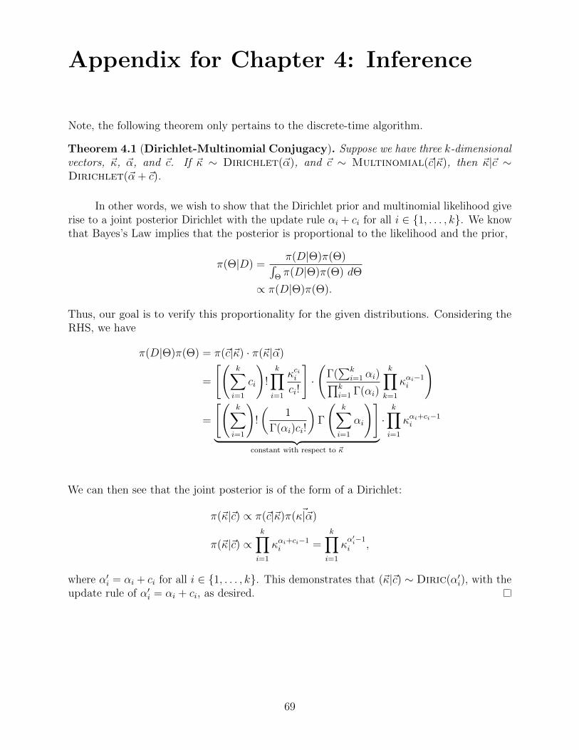
Appendix for Chapter 4: Inference

Note, the following theorem only pertains to the discrete-time algorithm.

Theorem 4.1 (Dirichlet-Multinomial Conjugacy). Suppose we have three k-dimensionalvectors, ~κ, ~α, and ~c. If ~κ ∼ Dirichlet(~α), and ~c ∼ Multinomial(~c|~κ), then ~κ|~c ∼Dirichlet(~α + ~c).

In other words, we wish to show that the Dirichlet prior and multinomial likelihood giverise to a joint posterior Dirichlet with the update rule αi + ci for all i ∈ {1, . . . , k}. We knowthat Bayes’s Law implies that the posterior is proportional to the likelihood and the prior,

π(Θ|D) =π(D|Θ)π(Θ)∫

Θπ(D|Θ)π(Θ) dΘ

∝ π(D|Θ)π(Θ).

Thus, our goal is to verify this proportionality for the given distributions. Considering theRHS, we have

π(D|Θ)π(Θ) = π(~c|~κ) · π(~κ|~α)

=

[(k∑i=1

ci

)!k∏i=1

κciici!

]·

(Γ(∑k

i=1 αi)∏ki=1 Γ(αi)

k∏k=1

καi−1i

)

=

[(k∑i=1

)!

(1

Γ(αi)ci!

)Γ

(k∑i=1

αi

)]︸ ︷︷ ︸

constant with respect to ~κ

·k∏i=1

καi+ci−1i

We can then see that the joint posterior is of the form of a Dirichlet:

π(~κ|~c) ∝ π(~c|~κ)π( ~κ|~α)

π(~κ|~c) ∝k∏i=1

καi+ci−1i =

k∏i=1

κα′i−1i ,

where α′i = αi + ci for all i ∈ {1, . . . , k}. This demonstrates that (~κ|~c) ∼ Diric(α′i), with theupdate rule of α′i = αi + ci, as desired.

69

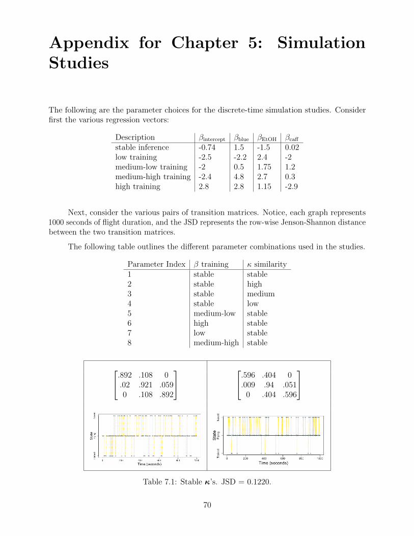
Appendix for Chapter 5: SimulationStudies

The following are the parameter choices for the discrete-time simulation studies. Considerfirst the various regression vectors:

Description βintercept βblue βEtOH βcaff

stable inference -0.74 1.5 -1.5 0.02low training -2.5 -2.2 2.4 -2medium-low training -2 0.5 1.75 1.2medium-high training -2.4 4.8 2.7 0.3high training 2.8 2.8 1.15 -2.9

Next, consider the various pairs of transition matrices. Notice, each graph represents1000 seconds of flight duration, and the JSD represents the row-wise Jenson-Shannon distancebetween the two transition matrices.

The following table outlines the different parameter combinations used in the studies.

Parameter Index β training κ similarity1 stable stable2 stable high3 stable medium4 stable low5 medium-low stable6 high stable7 low stable8 medium-high stable

.892 .108 0.02 .921 .0590 .108 .892

.596 .404 0.009 .94 .051

0 .404 .596

Table 7.1: Stable κ’s. JSD = 0.1220.

70

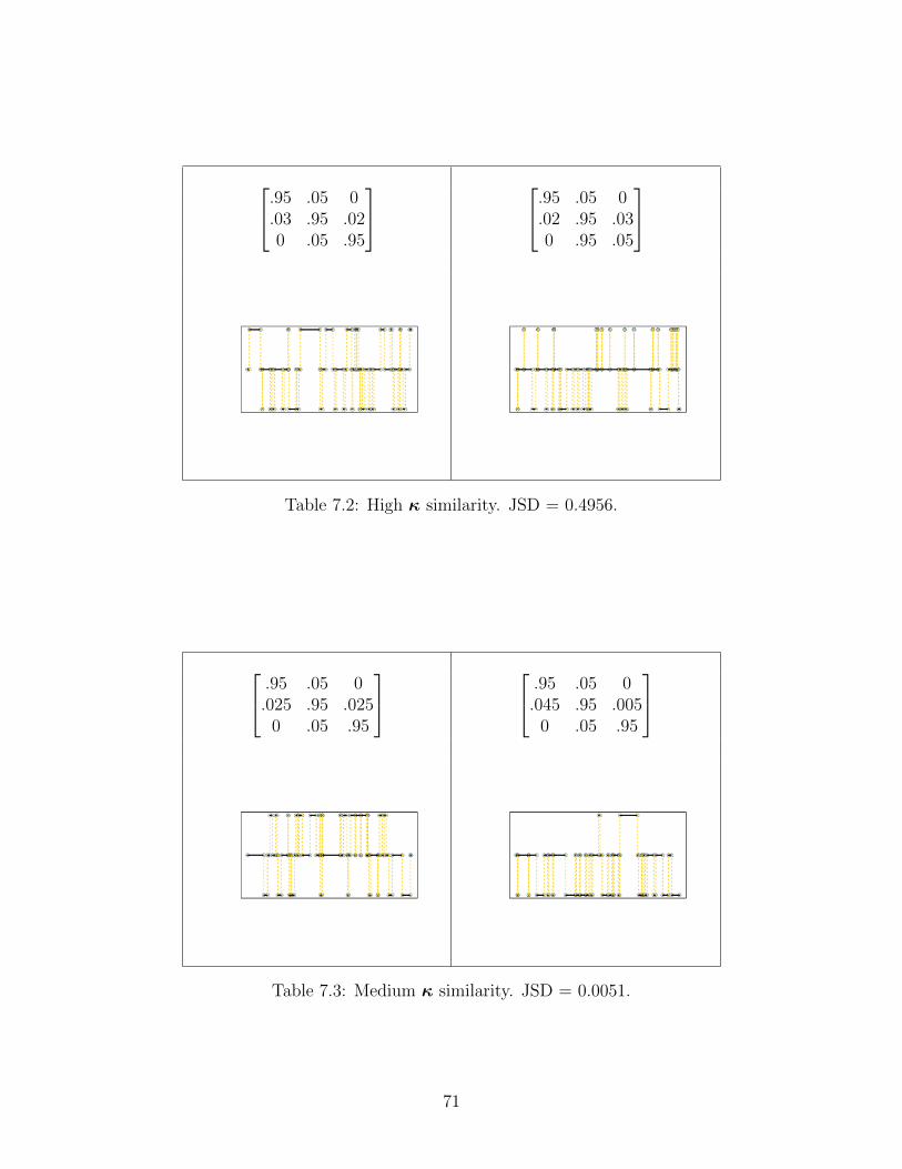
.95 .05 0.03 .95 .020 .05 .95

.95 .05 0.02 .95 .030 .95 .05

Table 7.2: High κ similarity. JSD = 0.4956.

.95 .05 0.025 .95 .025

0 .05 .95

.95 .05 0.045 .95 .005

0 .05 .95

Table 7.3: Medium κ similarity. JSD = 0.0051.

71

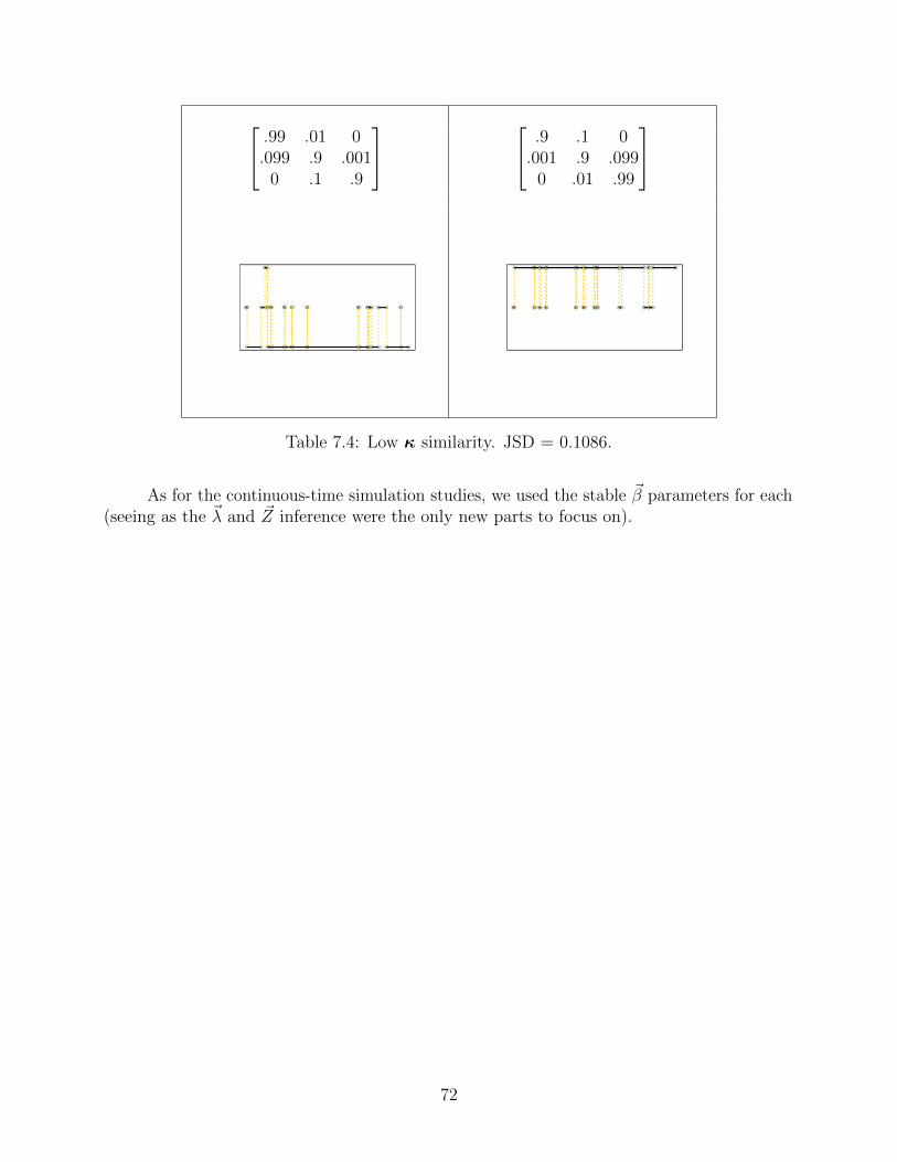
.99 .01 0.099 .9 .001

0 .1 .9

.9 .1 0.001 .9 .099

0 .01 .99

Table 7.4: Low κ similarity. JSD = 0.1086.

As for the continuous-time simulation studies, we used the stable ~β parameters for each(seeing as the ~λ and ~Z inference were the only new parts to focus on).

72

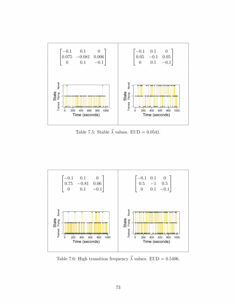
−0.1 0.1 00.075 −0.081 0.006

0 0.1 −0.1

−0.1 0.1 00.05 −0.1 0.05

0 0.1 −0.1

Table 7.5: Stable ~λ values. EUD = 0.0541.

−0.1 0.1 00.75 −0.81 0.06

0 0.1 −0.1

−0.1 0.1 00.5 −1 0.50 0.1 −0.1

Table 7.6: High transition frequency ~λ values. EUD = 0.5406.

73

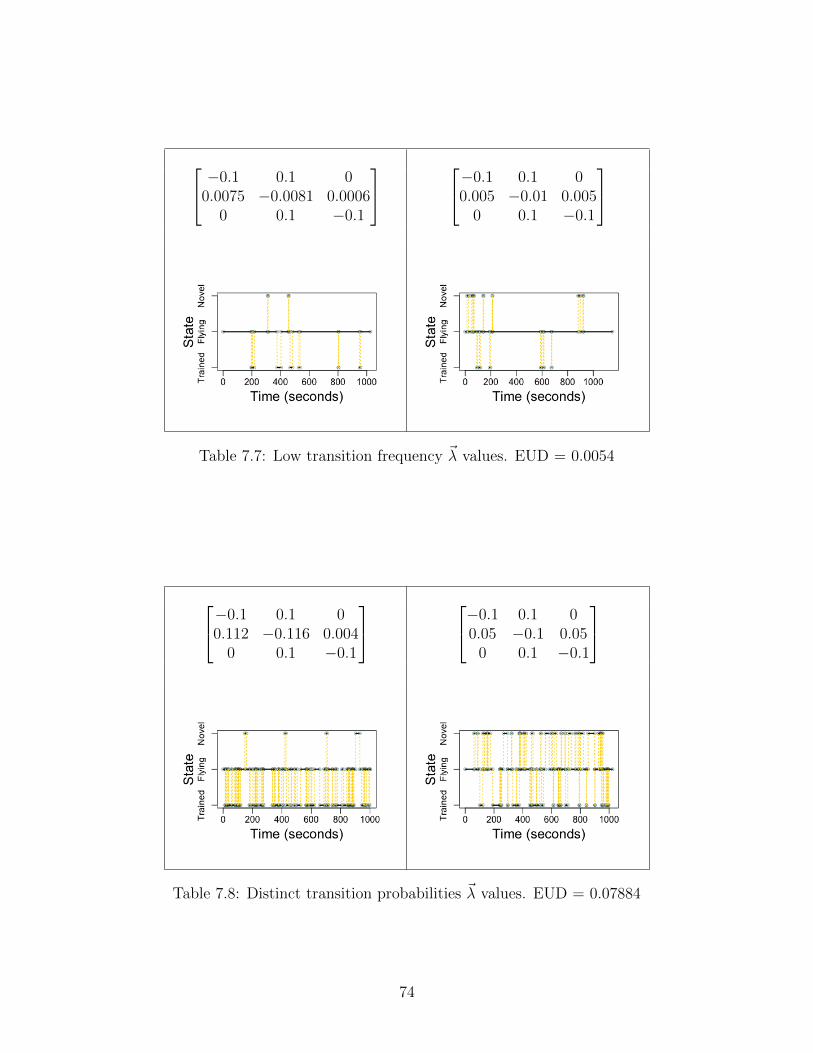
−0.1 0.1 00.0075 −0.0081 0.0006

0 0.1 −0.1

−0.1 0.1 00.005 −0.01 0.005

0 0.1 −0.1

Table 7.7: Low transition frequency ~λ values. EUD = 0.0054

−0.1 0.1 00.112 −0.116 0.004

0 0.1 −0.1

−0.1 0.1 00.05 −0.1 0.05

0 0.1 −0.1

Table 7.8: Distinct transition probabilities ~λ values. EUD = 0.07884

74

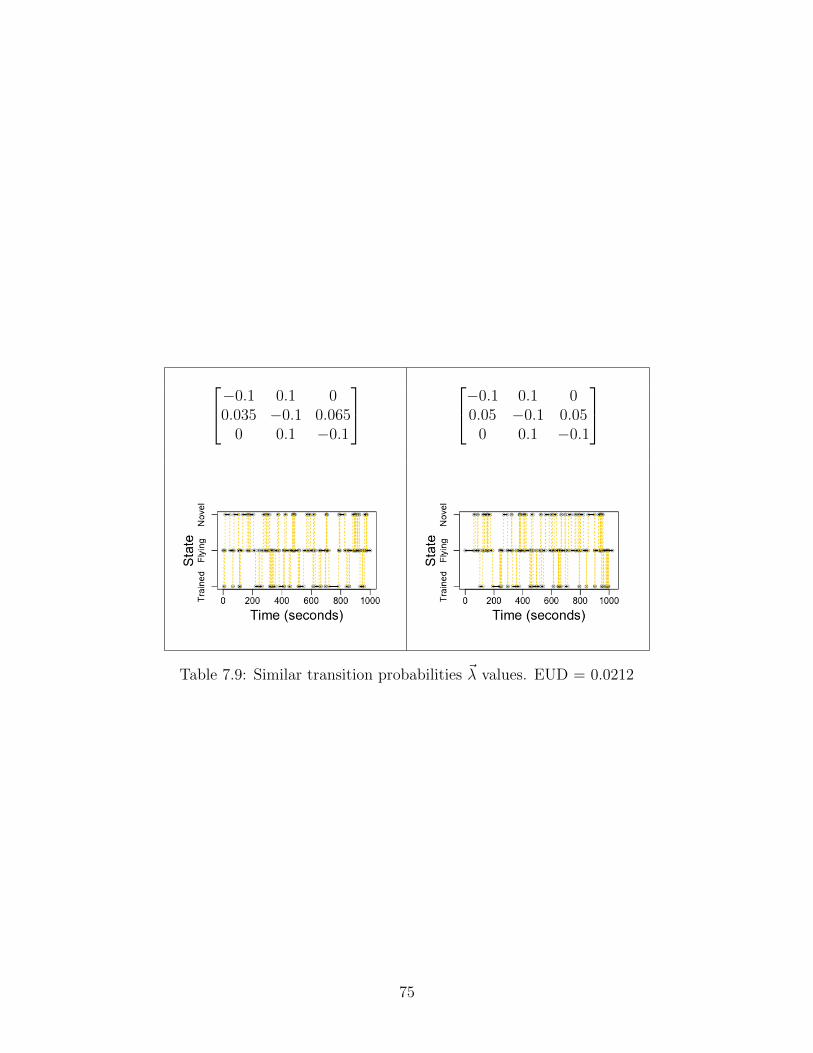
−0.1 0.1 00.035 −0.1 0.065

0 0.1 −0.1

−0.1 0.1 00.05 −0.1 0.05

0 0.1 −0.1

Table 7.9: Similar transition probabilities ~λ values. EUD = 0.0212

75

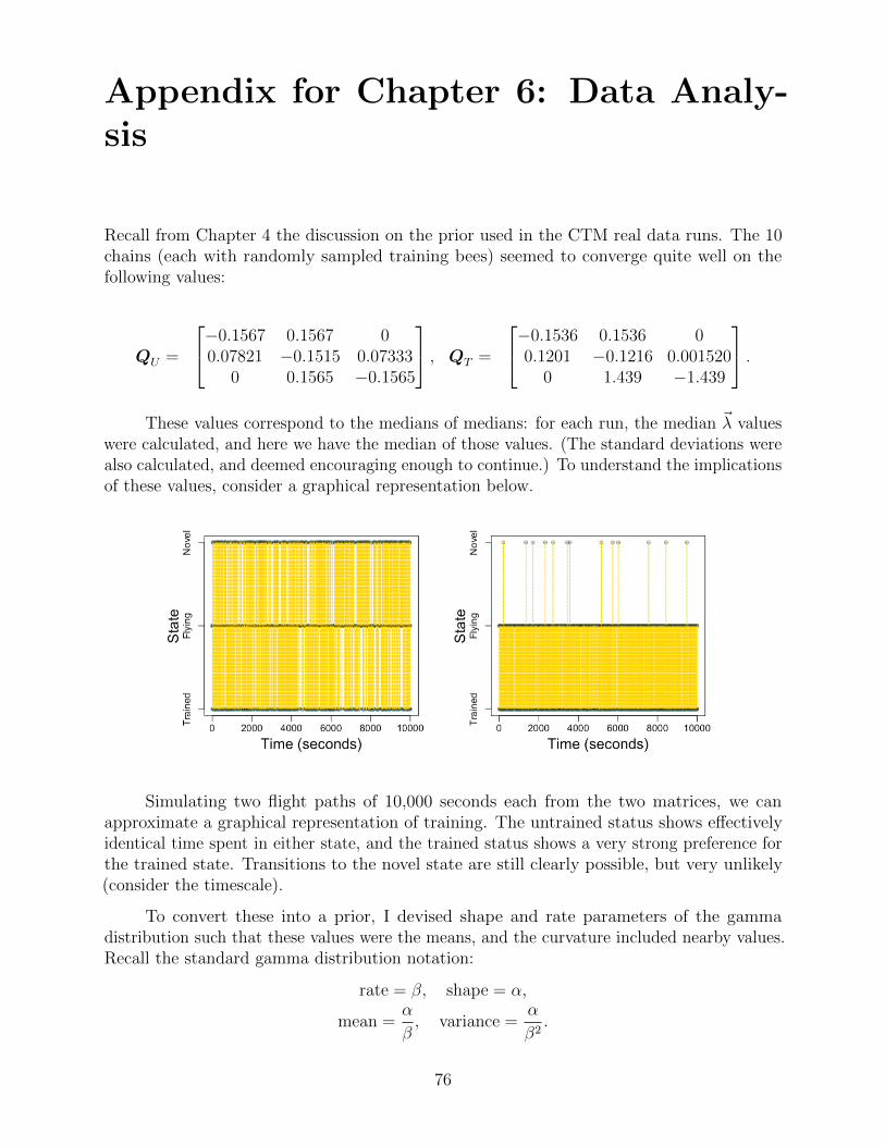
Appendix for Chapter 6: Data Analy-sis

Recall from Chapter 4 the discussion on the prior used in the CTM real data runs. The 10chains (each with randomly sampled training bees) seemed to converge quite well on thefollowing values:

QU =

−0.1567 0.1567 00.07821 −0.1515 0.07333

0 0.1565 −0.1565

, QT =

−0.1536 0.1536 00.1201 −0.1216 0.001520

0 1.439 −1.439

.These values correspond to the medians of medians: for each run, the median ~λ values

were calculated, and here we have the median of those values. (The standard deviations werealso calculated, and deemed encouraging enough to continue.) To understand the implicationsof these values, consider a graphical representation below.

Simulating two flight paths of 10,000 seconds each from the two matrices, we canapproximate a graphical representation of training. The untrained status shows effectivelyidentical time spent in either state, and the trained status shows a very strong preference forthe trained state. Transitions to the novel state are still clearly possible, but very unlikely(consider the timescale).

To convert these into a prior, I devised shape and rate parameters of the gammadistribution such that these values were the means, and the curvature included nearby values.Recall the standard gamma distribution notation:

rate = β, shape = α,

mean =α

β, variance =

α

β2.

76

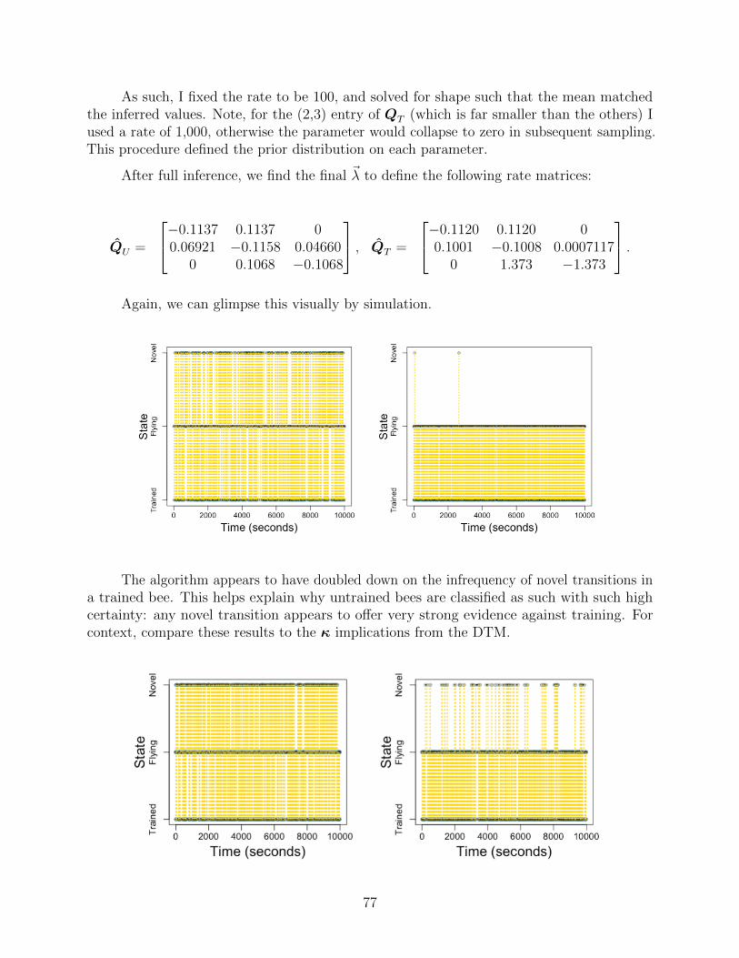
As such, I fixed the rate to be 100, and solved for shape such that the mean matchedthe inferred values. Note, for the (2,3) entry of QT (which is far smaller than the others) Iused a rate of 1,000, otherwise the parameter would collapse to zero in subsequent sampling.This procedure defined the prior distribution on each parameter.

After full inference, we find the final ~λ to define the following rate matrices:

Q̂U =

−0.1137 0.1137 00.06921 −0.1158 0.04660

0 0.1068 −0.1068

, Q̂T =

−0.1120 0.1120 00.1001 −0.1008 0.0007117

0 1.373 −1.373

.Again, we can glimpse this visually by simulation.

The algorithm appears to have doubled down on the infrequency of novel transitions ina trained bee. This helps explain why untrained bees are classified as such with such highcertainty: any novel transition appears to offer very strong evidence against training. Forcontext, compare these results to the κ implications from the DTM.

77

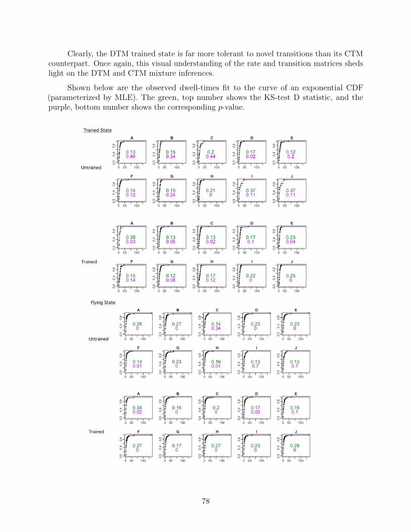
Clearly, the DTM trained state is far more tolerant to novel transitions than its CTMcounterpart. Once again, this visual understanding of the rate and transition matrices shedslight on the DTM and CTM mixture inferences.

Shown below are the observed dwell-times fit to the curve of an exponential CDF(parameterized by MLE). The green, top number shows the KS-test D statistic, and thepurple, bottom number shows the corresponding p-value.

78

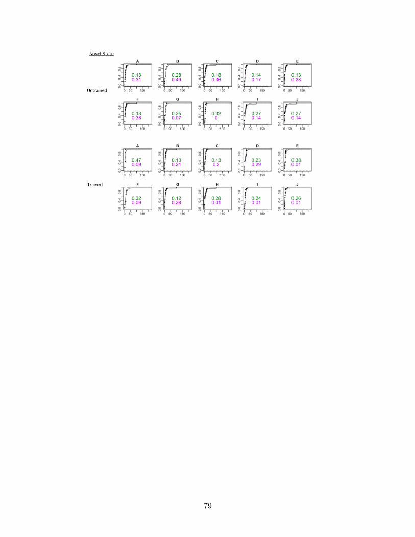
79

Bibliography

1. Ross, S. M. A First Course in Probability Fifth. isbn: 0137463146 9780137463145013895772X 9780138957728 (Prentice Hall, Upper Saddle River, N.J., 1998).

2. Dobrow, R. P. Introduction to stochastic processes with R eng. isbn: 1118740718 (JohnWiley and Sons, Inc., Hoboken, New Jersey, 2016).

3. Sigman, K. Lecture notes on Stochastic Modeling I 2009. http://www.ieor.columbia.edu/~sigman/stochastic-I.html.

4. Whitt, W. Continuous-time Markov chains. Dept. of Industrial Engineering and Opera-tions Research, Columbia University, New York (2006).

5. Hitchcock, D. B. A History of the Metropolis-Hastings Algorithm. The AmericanStatistician 57, 254–257. issn: 00031305. http://www.jstor.org/stable/30037292(2003).

6. Metropolis, N., Rosenbluth, A. W., Rosenbluth, M. N., Teller, A. H. & Teller, E. Equationof State Calculations by Fast Computing Machines. The Journal of Chemical Physics21, 1087–1092. https://doi.org/10.1063/1.1699114 (1953).

7. Hastings, W. K. Monte Carlo Sampling Methods Using Markov Chains and TheirApplications. Biometrika 57, 97–109. issn: 00063444. http://www.jstor.org/stable/2334940 (1970).

8. Gundersen, G. Feb. 2020. http://gregorygundersen.com/blog/2020/02/23/gibbs-sampling/.

9. Mathis, A. et al. Markerless tracking of user-defined features with deep learning. CoRRabs/1804.03142. arXiv: 1804.03142. http://arxiv.org/abs/1804.03142 (2018).

10. Introduction to Generalized Linear Mixed Models https://stats.idre.ucla.edu/

other/mult-pkg/introduction-to-generalized-linear-mixed-models/.

11. Mcculloch, C. E. & Neuhaus, J. M. in Wiley StatsRef: Statistics Reference Online (Amer-ican Cancer Society, 2014). isbn: 9781118445112. eprint: https://onlinelibrary.wiley.com/doi/pdf/10.1002/9781118445112.stat07540. https://onlinelibrary.wiley.com/doi/abs/10.1002/9781118445112.stat07540.

12. Visual acuity of the honey bee retina and the limits for feature detection. ScientificReports 7, 45972. https://doi.org/10.1038/srep45972 (2017).

13. Osborne, J. L. et al. Bumblebee flight distances in relation to the forage landscape.Journal of Animal Ecology 77, 406–415. eprint: https://besjournals.onlinelibrary.wiley.com/doi/pdf/10.1111/j.1365-2656.2007.01333.x. https://besjournals.onlinelibrary.wiley.com/doi/abs/10.1111/j.1365-2656.2007.01333.x (2008).

14. R Core Team. R: A Language and Environment for Statistical Computing R Foundationfor Statistical Computing (Vienna, Austria, 2019). https://www.R-project.org/.

15. Wickham, H. et al. Welcome to the tidyverse. Journal of Open Source Software 4, 1686(2019).

80

16. Jasra, A., Holmes, C. C. & Stephens, D. A. Markov Chain Monte Carlo Methods andthe Label Switching Problem in Bayesian Mixture Modeling. Statistical Science 20,50–67. https://doi.org/10.1214/088342305000000016 (2005).

17. Hoff, P. D. A First Course in Bayesian Statistical Methods 1st. isbn: 0387922997(Springer Publishing Company, Incorporated, 2009).

18. Endres, D. M. & Schindelin, J. E. A new metric for probability distributions. IEEETransactions on Information Theory 49, 1858–1860 (2003).

19. Gelman, A., Carlin, J. B., Stern, H. S. & Rubin, D. B. Bayesian Data Analysis 2nd ed.(Chapman and Hall/CRC, 2004).

20. Meng, X.-L. Posterior Predictive p-Values. The Annals of Statistics 22, 1142–1160. issn:00905364. http://www.jstor.org/stable/2242219 (1994).

21. Massey, F. J. The Kolmogorov-Smirnov Test for Goodness of Fit. Journal of the AmericanStatistical Association 46, 68–78. issn: 01621459. http://www.jstor.org/stable/2280095 (1951).

22. Betancourt, M. A Conceptual Introduction to Hamiltonian Monte Carlo 2018. arXiv:1701.02434 [stat.ME].

23. Wong, A. K. C. & You, M. Entropy and Distance of Random Graphs with Applicationto Structural Pattern Recognition. IEEE Transactions on Pattern Analysis and MachineIntelligence PAMI-7, 599–609 (1985).

24. Joe Blitzstein. Lecture 17: Moment Generating Functions. Harvard Stat 110 https:

//www.youtube.com/watch?v=N8O6zd6vTZ8&t=586s. Online; accessed 14 April 2021.2006.

81