A Bayesian approach for inverse modeling, data assimilation, and conditional simulation of spatial random fields

A Bayesian approach for inverse modeling, data assimilation,and conditional simulation of spatial random fields

Yoram Rubin,1 Xingyuan Chen,1 Haruko Murakami,2 and Melanie Hahn1

Received 20 October 2009; revised 16 February 2010; accepted 27 April 2010; published 6 October 2010.

[1] This paper addresses the inverse problem in spatially variable fields such as hydraulicconductivity in groundwater aquifers or rainfall intensity in hydrology. Common to all theseproblems is the existence of a complex pattern of spatial variability of the target variablesand observations, the multiple sources of data available for characterizing the fields, thecomplex relations between the observed and target variables and the multiple scales andfrequencies of the observations. The method of anchored distributions (MAD) that wepropose here is a general Bayesian method of inverse modeling of spatial random fields thataddresses this complexity. The central elements of MAD are a modular classification ofall relevant data and a new concept called “anchors.” Data types are classified by the waythey relate to the target variable, as either local or nonlocal and as either direct or indirect.Anchors are devices for localization of data: they are used to convert nonlocal, indirectdata into local distributions of the target variables. The target of the inversion is thederivation of the joint distribution of the anchors and structural parameters, conditional to allmeasurements, regardless of scale or frequency of measurement. The structural parametersdescribe large‐scale trends of the target variable fields, whereas the anchors capturelocal inhomogeneities. Following inversion, the joint distribution of anchors and structuralparameters is used for generating random fields of the target variable(s) that are conditionedon the nonlocal, indirect data through their anchor representation. We demonstrate MADthrough a detailed case study that assimilates point measurements of the conductivity withhead measurements from natural gradient flow. The resulting statistical distributions ofthe parameters are non‐Gaussian. Similarly, the moments of the estimates of the hydraulichead are non‐Gaussian.We provide an extended discussion ofMADvis à vis other inversionmethods, including maximum likelihood and maximum a posteriori with an emphasis onthe differences between MAD and the pilot points method.

Citation: Rubin, Y., X. Chen, H. Murakami, and M. Hahn (2010), A Bayesian approach for inverse modeling, data assimilation,and conditional simulation of spatial random fields, Water Resour. Res., 46, W10523, doi:10.1029/2009WR008799.

1. Introduction

[2] This paper presents a new approach for inverse mod-eling called method of anchored distributions (MAD). MADis an inverse method focused on estimating the distributionsof parameters in spatially variable fields. MAD addressesseveral of the main challenges facing inverse modeling.These challenges fall into two broad categories: data assim-ilation and modularity.[3] Data assimilation in inverse modeling is the challenge

of using multiple and complementary types of data as sourcesof information relevant to the target variable(s). In hydro-geological applications, for example, onemay be interested inmapping the spatial distribution of the hydraulic conductivityK [cf. Kitanidis and Vomvoris, 1983; Kitanidis, 1986, 1991,1995, 1997a, 1997b; Carrera and Neuman, 1986a, 1986b;

Hernandez et al., 2006] using measurements of the hydraulichead, measurements of concentrations and travel timesobtained from solute transport experiments [Bellin andRubin, 2004], and measurements of geophysical attributesobtained from geophysical surveys.[4] Another example is the mapping of ocean circulation,

which relies on a variety of data types (e.g., temperature,density, velocity vector components) obtained from shipsurveys, moored instruments, buoys drifting freely on orfloating below the ocean surface, and satellites. These dataare measured over a wide range of scales and frequencies,and they need to be assimilated to yield accurate circulationmodels.[5] In a third example, air quality management requires

constructing maps of dry deposition pollution levels. Ideally,such maps would be based on a dense network of monitoringstations, but generally such networks do not exist. Alternativeand related information must be used instead. For example,there are two main sources of information for dry depositionlevels in the United States: one is pollution measurements at a

1Department of Civil and Environmental Engineering, University ofCalifornia, Berkeley, California, USA.

2Department of Nuclear Engineering, University of California,Berkeley, California, USA.

Copyright 2010 by the American Geophysical Union.0043‐1397/10/2009WR008799

This article has been corrected because of errors introduced in theProduction Cycle.

WATER RESOURCES RESEARCH, VOL. 46, W10523, doi:10.1029/2009WR008799, 2010

W10523 1 of 23

sparse set of about 50 monitoring stations called CASTNet,with spacing between stations on the order of hundred ofkilometers, and the other is the output of regional scale airquality models with grid resolution on the order of a fewkilometers [Fuentes and Raftery, 2005].[6] In all these cases, the observations can be related to the

target variables by functions that relate measurement to targetvariables. The challenge in all these cases is to combinethe multiple sources of data into a coherent map of thetarget variables without introducing external factors such assmoothing and weighting.[7] To address such a wide range of problems we would

need to address the challenge of modularity. Modularitymeans an inverse modeling approach that is not tied to par-ticular models or data types and maintains the flexibilityto accommodate a wide range of models and data types.Inverse methodology and the numerical simulation of data‐generating processes have become very closely intertwined,in a way that makes them very limited in applications. (“Data‐generating processes” in this document refers to the naturalprocesses that result in a quantity being measured. Theseprocesses are usually simulated by numerical codes.) This canbe attributed to the increasing complexity of the processesthat are being analyzed and of the computational techniquesneeded for their analysis. For example, inverse modeling inhydrogeology evolved from Theis’ type‐curve matching intomodern studies that include complex and specialized ele-ments such as (1) adaptive and parallel computing techniques,(2) geophysical modeling of electromagnetic fields and of thepropagation of seismic waves, and (3) complex multi com-ponent chemical reactions. The range of skills needed forimplementing these elements forced researchers to build theinversion procedure around their own or favorite numericalcodes. As a result, the potential for expanding the rangeof applications beyond the original application, for example,by changing the data types or the numerical models used,is limited. Modularity is a strategy for alleviating this diffi-culty by pursuing a model‐independent inverse modelingframework.[8] This paper, through presentation of the MAD concept,

explores all these issues using a Bayesian framework. Atheoretical approach is developed and demonstrated with twosubsurface flow problems.

2. Data Classification and Anchor Definitions

[9] This section presents several of the principles under-lying the MAD concept. It summarizes for completeness andexpands a few developments included in an unpublishedmanuscript by Zhang and Rubin (Inverse modeling of spatialrandom fields, unpublished manuscript, 2008) and in a con-ference presentation by Zhang and Rubin [2008]. The MADapproach to inverse modeling is built around two elements.The first element is data classification. The second element isa strategy for localization of nonlocal data. The localizationstrategy intends to create a unified approach for dealing withall types of data. These two elements are integrated into (1) aBayesian formalism for data assimilation and (2) a forwardmodeling strategy in the form of conditional simulation. Theintegration of these two elements is done in a modular formthat can accommodate a wide variety of data types andmultiple ways in which these data can be related to the targetvariables of interest. The rationale for formulating the inverse

problem using a statistical formalism has been amply dis-cussed in the literature [e.g., Kitanidis, 1986; Rubin, 2003]and is not repeated here for the sake of brevity.[10] We consider a spatial random process denoted by Y(x),

where x is the space coordinate. As discussed earlier, Y couldbe a variable in any number of fields. It could represent, forexample, the hydraulic conductivity in hydrogeologicalapplications. In this case, inverse modeling would focus onthe conductivity field based on measurements of pressureinduced by a pumping test, concentration data from a tracerexperiment, or the arrival times of seismic waves at multiplelocations obtained from a geophysical survey [Hoverstenet al., 2006; Hou et al., 2006]. The entire field of Y isdenoted by ~Y . A realization of ~Y is denoted by ~y. Given data zthat is related to ~y, the goal is to derive the conditional dis-tribution of the field, p(~y|z), and to generate random samplesfrom that distribution.[11] The ~Y field is defined through a vector of model

parameters (q, J). The q part of this vector includes a set ofparameters that are designed to capture the global trends of Y,and it can assume different forms. For example, if one selectsa geostatistical approach for modeling the global trends of Y[cf. Rubin and Seong, 1994; Seong and Rubin, 1999], qwould include parameters such as the mean of Y and theparameters of its spatial covariance. An alternative formula-tion of q could involve a zonation‐based approach [e.g.,Poeter and Hill, 1997], whereby q includes the values of Yat various zones of the model domain. It could also be ahybrid approach of these two concepts, whereby the modeldomain is subdivided into geological units, with each of thegeological units characterized by a different geostatisticalmodel [cf. Rubin, 1995; Dai et al., 2004; Ritzi et al., 2004;Rubin et al., 2006]. The J component of this vector consistsof the anchored distributions. Anchored distributions oranchors, in short, are devices used to capture the local effectsor, in other words, all the elements or features of ~Y that cannotbe captured using the global parameters represented by q(provided that the local effects have an impact on the data). Intheir simplest form, anchors would be error‐free measure-ments of Y. Other forms of anchors include measurements ofY coupled with error distributions and/or anchors that areobtained by inversion. The anchors are defined in detail insection 2.2.[12] The overall strategy for deriving p(~yjz) is to derive

a joint conditional distribution of the model parameters,p(q, Jjz), which would in turn allow us to generate multiplerealizations of ~Y that maintain the global trends and capturethe local effects. The distribution p(q, Jjz) should be generaland flexible enough to accommodate a wide range of for-mulations of the vector (q, J), as well as a wide range of datatypes that could be folded into the vector z.

2.1. Data Classification

[13] The concept of anchors is built around a generalapproach for classifying data based on the relation of the datato the attribute y and the support volumes of the data and theattribute. There are two classifiers that are commonly used todescribe such relationships: local and nonlocal. Data could bemeasured over the same support as y and be modeled as afunction of the collocated y, and in this case, wewould refer tothem as local. Otherwise, they would be nonlocal. As we willshow below, these relations could be captured using anchors.

RUBIN ET AL.: METHOD OF ANCHORED DISTRIBUTIONS W10523W10523

2 of 23

Weshall refer to local and nonlocal data as TypeA andTypeB,respectively, and we will use za and zb to denote the Type Aand Type B data, respectively. The vectors za and zb aregeneral symbols for data and may include any or all of thefollowing: measurements, descriptions of statistical rela-tions, and measurement errors. Type A and Type B datarefer to on‐site data. Information in the form of expertopinion or from similar fields is treated differently fallsunder the category of prior information.[14] Type A data can be related to y through the equation,

za ¼ y xað Þ þ ea; ð1Þ

where y is a known function and ea is a vector of length na ofzero‐mean errors. The vector za could include measurementsof Y, and in that case ea would represent measurement error. Itcan include predictions of y obtained by regression or throughthe use of petrophysical models [cf. Ezzedine et al., 1999],and in that case ea would represent regression or modelingerror. In the case where y is permeability, for example, TypeA data could include measurements of permeability obtainedusing permeameters or predicted permeability from soil tex-ture and grain size distributions using petrophysical models[cf. Ezzedine et al., 1999; Mavko et al., 1998].[15] Type B data include all the data that cannot be clas-

sified as Type A. Type B data are functions of the y field or asection of it that is larger than the volume support of the ymeasurement defined by TypeA data. The Type B data can bedescribed by the following equation,

zb ¼ M ~yð Þ þ eb; ð2Þ

where M is a known function, numerical or analytical, of thespatial field, representing one or more physical processes, andeb is a vector of length nb zero‐mean errors. It is recalled thatthe tilde sign over a variable denotes a field of that variable.The vector zb can include a wide range of data types thatcould be obtained from multiple sources. In hydrogeologicalapplications, zb could include data obtained from small‐ andlarge‐scale pumping tests, solute transport experiments,continuous observations of hydraulic heads, and geophysicalsurveys. With data from multiple sources, M in equation (2)should be viewed as a collective name for all models thatrelate the data to ~y, including, for example, flow and trans-port simulators and geophysical simulators.

2.2. The Concept of Anchors

[16] With Type A and Type B data available, the inver-sion’s final goal becomes the generation of Y fields condi-tioned on both data types. This could be done through theconditional distribution p(~yjza, zb). The major challenge inderiving this distribution is the absence of a simple devicethat would guarantee that the simulated/generated fields arealready conditioned on the Type B data. This would save theneed to verify that the generated fields are conditioned on theType B data without repeated use of M. We will constructsuch a device in the form of anchors.[17] Anchors are model devices in the form of local sta-

tistical distributions of Y, intended to establish connectionsbetween the unknown Y field and the data z = (za, zb). Usinganchors and structural parameters, we will be able to generateY fields that are conditioned on Type A and Type B data aswell as on the inferred distributions of the structural param-

eters. Conceptually, structural parameters describe globaltrends and spatial associations, whereas anchors capture localfeatures. We should emphasize at this point that anchorsare not pilot points. There are fundamental conceptual andtechnical differences that are discussed in great details insection 8.[18] Anchors are always given as statistical distributions,

but there is a different correspondence between anchors andType A data than for anchors and Type B data. In the case ofType A data, anchors are given in the form of statisticaldistributions representing the Y values plus measurement(or regression) error, and we have one anchor per one Type Ameasurement. Type B measurements, on the other hand,could be represented by more than one anchor, with eachanchor possibly corresponding to one or several Type Bmeasurements. Anchors are planted at multiple locations,with the idea that they would capture the informationcontained in the Type B measurements that is relevant to theY field. This is achieved by transforming the Type B data intomultiple anchors at known locations based on our knowledgeof the Y field and the nonlocal data generation process M.The transformation of Type B data into anchors changes boththe form of the data as well as the location of the information.Subsequently, simulations conditioned on these anchors are,to a large degree, conditioned on both Type A and Type Bdata.[19] Anchor placement is an important element of MAD:

obviously, we would want to place the anchors such that theycapture all the relevant information contained in the data. Thisis trivial for Type A data because in that case the anchors arecollocated with the measurements. It is a complex issue in thecase of Type B data because of the complex averaging appliedon Y by the Type B process. This issue will be discussed insection 6. Leaving the anchor placement question aside fornow, we will proceed to discuss how the statistical distribu-tions are determined for a given set of anchor locations.[20] In our approach, the anchors are viewed as model

parameters, similar to the structural parameters, and as such,will be determined by inversion. Denote the vector of anchorsby J = (Ja, Jb), where Ja, located at known locations xa,are the anchors corresponding to Type A data, whereas Jb,located at chosen locations xb, are the anchors correspondingto Type B data. The goal of the inversion is to derive the jointanchor‐parameter distribution p(q, Jjza, zb). Once this dis-tribution is defined, any random draw of (q, J) from thisdistribution contains all the information needed for generat-ing conditional realizations. The derivation of this distribu-tion is the subject of section 2.2.1.2.2.1. MAD With Type A and Type B Data[21] Whereas MAD in general uses both Type A and

Type B data, it also can be used for inverse modeling whenonly Type A or Type B data are available. These cases arepresented in this section. As a starting point, let us considerthe derivation of p(q, Jjza, zb), the joint distribution ofthe model parameters, including structural parameters andanchors, conditional to Type A and Type B data. Followingthe anchor notations defined in the previous section, it canbe shown that

p q;Jjza; zbð Þ / p q;Jjzað Þp zbjq;J; zað Þ¼ p Jajzað Þp qjJa; zað Þp Jbjq;Ja; zað Þp zbjq;J; zað Þ¼ p Jajzað Þp qjJað Þp Jbjq;Jað Þp zbjq;Jð Þ: ð3Þ

RUBIN ET AL.: METHOD OF ANCHORED DISTRIBUTIONS W10523W10523

3 of 23

Equation (3) is a Bayesian model that relates model para-meters to data and to prior information in the form of a pos-terior probability. In equation (3), the posterior probability issimplified by dropping za whenever it is coupled with Ja asconditions (i.e., to the right of ‘|’), under the assumption thatthe information provided by the anchors Ja encapsulates theinformation provided by za, thus rendering the conditioningon za superfluous.[22] In equation (3), p(zbjq, J) denotes the likelihood of

the Type B data, which is the key for relating the posteriordistribution of the model parameters with the Type B data.p(q, Jjza) has the dual role of being the posterior probabilitygiven Type A data, as well as a prior probability, precedingthe introduction of Type B data. The distribution p(Jajza)is derived from the Type A data. The distribution p(qjJa) isdiscussed in section 3.1 below. The distribution p(Jbjq, Ja)is the prior of the anchors Jb given Type A data and thestructural parameters vector q.[23] Equation (3) highlights the role of the anchored dis-

tribution as the mechanism for connecting between Type Aand Type B data, without making any specific modelingassumption to relate them. The only opening in equation (3)for ambiguity is in the relationships between the variousType B data that are included in the likelihood functionand the target variables. This can be dealt with in one of twoways. First, this relationship may be known or can safely beassumed or derived from physical principles using statisticalmodeling assumptions [cf. Hoeksema and Kitanidis, 1984;Dagan, 1985; Rubin and Dagan, 1987a, 1987b]. Otherwise,the likelihood function can be defined nonparametrically andderived numerically based on extensive numerical simula-tions. Both approaches can be implemented in MAD. In thecase study pursued here, we employed the second option.2.2.2. MAD With Type A Data Only[24] In the presence of Type A data only, equation (3)

simplifies to

p q;Jajzað Þ ¼ p Jajzað Þp qjJað Þ: ð4Þ

Since Type A data is local, the role of the anchors here islimited to modeling measurement or regression errors, andso the anchors here are measured or regressed, unlike theanchors corresponding to Type B data, which are inverted.[25] The distribution p(Jajza) represents the probabilities

of the various ensembles of anchor values that are plausiblein light of the Type A data and the distribution of themeasurement/regression errors. These ensembles can lead tovarious structural parameter combinations that are summa-rized in the distribution p(qjJa).[26] If a prior distribution for q is available [seeWoodbury

and Rubin, 2000;Hou and Rubin, 2005;Kass andWasserman,1996], we could use p(qjJa) / p(Jajq)p(q) to accommodatethe prior.[27] The application of MAD in this case includes a

sequence of three steps. First, the anchor distributions need tobe defined. Working with Type A data, the anchors are notobtained by inversion: they are determined based on themeasurement and/or regression errors. At the next step thedistribution of q is to be determined based on Ja [e.g.,Hoeksema and Kitanidis, 1984; Kitanidis, 1986; Diggle andRibeiro, 2006] and in the final step, this distribution is usedin conjunction with za to generate realizations of the Y fieldfrom the distribution p(~yjq, za).

[28] When the Type A data are error‐free, equation (4)could be simplified by noting that in this case the anchorsare equal to the measurements. In this case, the anchornotation could be ignored altogether, and the posterior dis-tribution of the structural parameters is given by

p qjzað Þ ¼ czap qð Þp zajqð Þ; ð5Þ

where p(q) is the prior distribution of the structural param-eters vector, p(zajq) is the likelihood and cza is a normalizingfactor. This case is in line with the studies of [e.g., Hoeksemaand Kitanidis, 1984; Michalak and Kitanidis, 2003].[29] The final step of this process consists of generating

realizations from the conditional distribution p(~yjza). Inthe studies cited in the previous paragraph, the distributionp(~yjq, za) was obtained by standard conditioning proceduresfor multivariate normal distributions. Distributions other thanmultivariate normal could also be used. Diggle and Ribeiro[2006] used trans‐Gaussian transforms to deal with non-normal distributions.2.2.3. MAD With Type B Data Only[30] In the absence of Type A data, equation (3) simplifies

as follows: p(Jajza)p(qjJa) becomes p(q). Next, p(Jbjq, Ja)becomes p(Jbjq). Finally, p(zbjq, J) becomes p(zbjq, Jb),leading to the following definition of the posterior,

p q;Jbjzbð Þ / p qð Þp Jbjqð Þp zbjq;Jbð Þ; ð6Þ

with the main difference compared to the previous cases isthat the prior is not informed by the Type A data.

3. Inverse Modeling With MAD

[31] The critical elements in application of equation (3)include the following: determination of the prior, the place-ment of the anchors, the derivation of the likelihood functionand the application of MAD for predictions. In this section,we discuss these elements individually (except the anchorplacement issue, which is discussed in section 5), and thenwe will show how they combine together into a modularalgorithm.

3.1. The Prior

[32] The prior for the entire model appears indirectly inequation (3) through the relation p(qjJa)/ p(q)p(Jajq). Theprior p(q) summarizes the information that is available on qprior to taking any measurements at the site or by ignoringthem. There is a large number of alternatives that could beused here. Broad statistical perspective is provided by Kassand Wasserman [1996], Woodbury and Ulrych, [1993],Woodbury and Rubin [2000], Hou and Rubin [2005], andDiggle and Ribeiro [2006]. There are many ideas on howto model the prior, and they can all be implemented here, atthe modeler’s discretion.

3.2. Modeling of the Likelihood

[33] An extensive body of literature is devoted to esti-mating multidimensional distributions that could be used forestimating the likelihood [cf. Scott and Sain, 2005]. As inthe case of the prior, there are multiple strategies that onecould pursue here. These strategies fall in general into twocategories: parametric and nonparametric. In the parametric

RUBIN ET AL.: METHOD OF ANCHORED DISTRIBUTIONS W10523W10523

4 of 23

approach, the likelihood model is postulated, leaving only theneed to estimate its parameters. In many cases, a normaldistribution is adopted for the likelihood [cf. Dagan, 1985;Carrera and Neuman, 1986a, 1986b; Hoeksema andKitanidis, 1984; Kitanidis, 1986; Rubin and Dagan, 1987a,1987b].[34] The nonparametric approach is more general because

it covers a wide range of distributions. The appeal of non-parametric methods lies in their ability to reveal structure inthe data that might be missed by parametric methods. Thisadvantage could be associated with a heavy price tag: non-parametric methods are often much more computationallydemanding than their parametric counterparts. The MADalgorithm (see next section) is flexible in its ability to employboth parametric and nonparametric methods. Several alter-natives for calculating the likelihood function are sum-marized in the work of Scott and Sain [2005] and Newtonand Raftery [1994]. For the particular applications dis-cussed below, we employed the algorithms described byHayfield and Racine [2008], which are part of the R‐Package[R Development Core Team, 2007].[35] Both approaches are suitable for MAD and can be

implemented at the modeler’s discretion. The overridingconsideration should be the selection of the most appropriaterepresentation of the likelihood, and this depends on the data.For example, when zb is composed of pressure head mea-surements measured in a uniform‐in‐the‐average flow in anaquifer domain characterized by small variance of the logconductivity, a multivariate normal likelihood function isappropriate because the head can be expressed as linearfunction of the log conductivity [Dagan, 1985]. We selectedto present here a nonparametric approach because it is more

general and because it is not commonly used in groundwaterapplications.[36] The likelihood p(zbjq, J) in equation (3) is estimated

using numerical simulations, as follows. For any given (q,J),we generate multiple conditional realizations of the Y field;with each realization, a forward model provides a predictionof zb in the form of ~zb. In other words, zb is viewed as ameasured outcome from random process, whereas ~zb is oneof many possible realizations, each corresponding to aparticular realization of (q, J). The ensemble of ~zb consti-tutes a sample of zb, and it is used for estimating the like-lihood at zb.[37] Nonparametric estimation of statistical distributions

requires a large number of forward simulations. When mul-tiple data types are involved, that would include conditionalsimulation of the Y field followed by forward modeling. InMAD, there are two elements that combine to reduce thecomputational effort. First, we do not need to evaluate thelikelihood p(zbjq, J) for every possible combination of zbvalues, but only for the particular set of values that weremeasured, thus requiring a smaller number of samples toensure convergence. Second, the dimension of the parametersvector (q, J) is small compared to full‐grid inversion.

3.3. A Flowchart for MAD

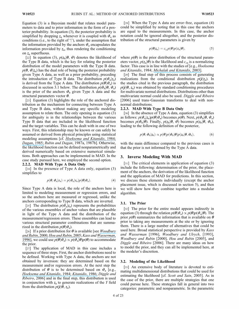
[38] The MAD approach is represented schematically inFigure 1, using the notation provided in equation (3). Figure 1shows the modular structure of the MAD approach. There arethree blocks in MAD, labeled Blocks I, II, and III, respec-tively, and two auxiliary blocks, labeled Auxiliary Blocks Aand B.

Figure 1. Graphical representation of the MAD approach. Anchors here refer to both Type A and Type Banchors (with variations depending on the application). Forward simulations in Block II refer to simulationsneeded for estimating the likelihood (see section 3.3).

RUBIN ET AL.: METHOD OF ANCHORED DISTRIBUTIONS W10523W10523

5 of 23

3.3.1. Block I[39] Block I is the preprocessing module, and it is focused

on the Type A data. It computes the joint distribution ofstructural parameters (q) and anchors (J) based on the TypeA data as well as any prior knowledge on the parameter vectorq. As noted earlier, there is a wide range of ideas that could beimplemented through this block. There is no particularapproach to modeling the prior that is hard‐wired intoMAD. The output of Block I is the conditional distributionp(q, Jjza), which is the posterior distribution of q withrespect to za. If we view zb as the “main” data, then thisprovides a prior of (q,J) for the Bayesian analysis of zb that iscarried out in Block II.3.3.2. Block II[40] Block II is the likelihood analysis module. It in-

corporates Type B data through the likelihood functionp(zbjq, J). When combined with the Block I product,p(q, Jjza), where J are the anchor values at locations xu, ityields the posterior p(q, Jjza, zb). The likelihood functionp(zbjq, J) is linked to observations by a forward model M,through the relationship zb = M(~y) + e. This relationship iscomposed of two elements: random field generation andforward simulation. The joint distribution of J and q fromBlock I is used to generate conditional realizations of the Yfield ~y. With each realization, the forward modelM generatesa realization of the Type B data that would eventually be partof the ensemble used to evaluate the likelihood function.Several forward models can be employed simultaneously,depending on the number of different Type B data employedin the inversion process, as indicated by the vertical barlinked to forward simulations. Examples for M functionsinclude flow models, solute fate and transport models, andgeophysical models. The positioning of Models I and IIwithin Block II and the positioning of Models III, IV asexternal but linkable elements to Block II intend to signifythe flexibility to plug in user‐supplied models in addition tohard‐wired models.3.3.3. Block III[41] Block III is the prediction block. It covers the post-

inversion analyses needed for predicting a future, unknownprocess of interest. It can connect directly to Block I inthe absence of Type B data. The forward simulation stepin Block III can guide the selection of anchor locations inBlock II. A simple way to do it is by evaluating alterna-tive anchor placement schemes. As with the other blocks,Block III could be linked with a wide range of forward sim-ulation codes and computational techniques.[42] The prediction block is built around multiple condi-

tional realizations of the random field. Each of these reali-zations is generated using a realization of parameters andanchors drawn from the joint distribution of q and J. Gen-erating random fields from the joint distribution of q and J isadvantageous because many alternative combinations of bothJ and q could be evaluated, leading to a more completecharacterization of uncertainties associated with the model.This is in contrast to the commonly usedmaximum likelihood(ML) or maximum a posteriori (MAP) approaches, both ofwhich present the uncertainties of Y corresponding to a fixedset of the model parameters.[43] The auxiliary blocks include Block A, which is dedi-

cated for anchor placement analysis, and Block B, which isdedicated for model inter‐comparison (both topics are dis-cussed in the next section). They are not considered as core

blocks because they contain elective procedures that are notabsolutely necessary for a complete application of MAD.

4. Measurement Errors, Parametric Errors,and Conceptual Modeling Errors

[44] An important element of any inverse modeling,including MAD, is the forward model M. Once a realizationof Y is generated in the form of a field ~y, M(~y) could be usedto generate the field or possibly a number of fields ~zb,corresponding to all Type B attributes. A subset of ~zb,specifically those values generated at xb, could be used toconstruct a sample of the likelihood p(zbjq, J). One canreasonably expect that the values generated by M(~y) at xbwould be different from zb, because of parametric errors,conceptual modeling errors, numerical modeling errors andmeasurement errors. Parametric error refers to estimationerrors in the parameters of a particularM, whereas conceptualmodeling errors refer to errors in formulating the conceptsthat underlie the model M.[45] It is recalled that equation (1) defines the mea-

surement/regression error associated with Type A data.Equation (2) defines the errors associated with Type B datadue to measurement and parameter errors for a given modelM. By introducing these errors into equation (3), we couldaccount explicitly for the impact of these errors on the pos-terior distribution. equation (3) could be expanded to includethe error terms as follows:

p q;Jjza; zbð Þ /Z

p Jajya; eað Þp qjJað Þp Jbjq;Jað Þ� p zbjq;J; ebð Þp eð Þde: ð7Þ

The error in the Type A data is represented by ea. Theparameter error is represented by eb, and it covers errors inJb

and in the structural parameters q. e = (ea, eb) and p(e)denotes its distribution. p(Jajya, ea) is the distribution ofanchors given measured (or regressed) Y values and the dis-tribution of the measurement/regression errors.[46] For demonstration, consider the case of zero error in

the Type A data. This distribution becomes the Dirac functionp(Jajya, ea) = d(Ja − ya), which means that the anchorscorresponding to the Type A data are equal to the measuredvalues. On the basis of that, equation (7) becomes:

p q;Jjza; zbð Þ / p qjyað Þp Jbj�; yað ÞZ

p zbjq;Jb; ya; ebð Þp ebð Þdeb:

Equation (7) does not account for the errors associated withthe formulation of M, because it considers only a single,deterministically known modelM, and thus, we cannot knowhow M would compare against the perfect, error‐free model(which in itself is an elusive concept). Note that a “deter-ministically known” model does not exclude from con-sideration parameter errors, it only assumes that the modelformulation is taken to be correct.[47] One idea on how to depart from the confines of a

single model is to formulate and evaluate several alternativeand plausible models and with this minimize the risk impliedby betting on a single model. This is the approach pursued byHoeting et al. [1999], Neuman [2003], and Ye et al. [2008],which we apply here for the MAD algorithm. The idea hereis to formulate N alternative forward models: Mi, i = 1, .., N.

RUBIN ET AL.: METHOD OF ANCHORED DISTRIBUTIONS W10523W10523

6 of 23

Each alternative model is defined by a different set ofparameters: a model Mi is defined by a corresponding set ofparameters (qi,Ji).N could be large, reflecting thewide rangeof choices that could be made in the model formulationprocess. Such choices could include, for example, the selec-tion of a particular correlation model for Y or selecting aparticular multivariate distribution of Y from several availablealternatives. These choices could also reflect decisions aboutnumerical implementation, such as the selection of grid sizeand time step.[48] Alternative models imply alternative combinations

of structural parameters and anchors. Assuming thatMi, i = 1, ..,N, are theNmodels under consideration and qi,Ji

are the set of parameters corresponding to Mi, equation (3)and each of its derivatives (e.g., equation (7)) could bewritten for each of the N combinations qi, Ji instead of asingle q, J combination. Solving the inverse problem wouldmean deriving the posterior distribution for each of thesecombinations.[49] To account for the multiple models in predictions,

each of these models need to be weighted by a probability

p(Mi) such thatPNi¼1

p(Mi) = 1. The role of p(Mi) is to reflect the

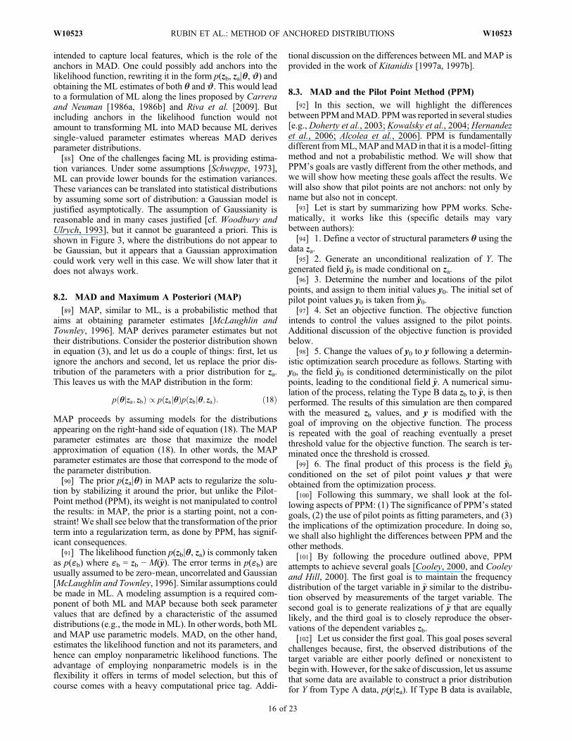
plausibility of the corresponding model. With these defini-tions, any variable of interest can be predicted in a variety ofways. For example, one could average the expected valueof variable y at the maximum likelihood point of each ofthe models using hyi = P

iy(M̂ i)p(M̂ i) where ^ denotes the

maximum likelihood point. The major challenge here is todetermine the model probabilities p(Mi). Derivation of theprobabilities p(Mi), i = 1, .., N, is pursued by Hoeting et al.[1999], Neuman [2003], and Ye et al. [2008]. In our sub-sequent discussion, we shall refer to this approach as thediscrete model approach.[50] In the discrete approach, each of the models Mi is

defined by a different set of parameters qi, Ji and a proba-bility p(Mi). Defining the likelihood functions requires acomputational effort that scales up with the number of modelsand the number of parameters in eachmodel. This effort couldbe reduced if parameters could be used to distinguish betweenconceptual models. We refer to this idea as broad spectrummodel selection because a single parameter could be used torepresent a broad spectrum of models. It can complementdiscrete model selection or replace it, depending on theapplication.[51] To demonstrate this idea, we will consider the selec-

tion of the spatial covariance of Y. The literature suggestsseveral authorized covariance models, e.g., normal, expo-nential, etc. Combinations of authorized models are alsolikely candidates. For each case one could consider isotropicand anisotropic models [Rubin, 2003, chapter 2]. One caneasily identify N alternative models that could be used inequation (4), and each of them could be associated with aprobability p(Mi). Representing all or a subset of thesealternatives using equation (4) is a possibility, as discussedearlier. The alternative we propose here is to consider theMatérn family of covariance functions [Matérn, 1986], givenby [cf. Nowak et al., 2010]

c ‘ð Þ ¼ �2

2��1G �ð Þ ‘ð Þ�B� ‘ð Þ; ð8Þ

where ‘2 =Pnsi¼1

(ri /li)2, ri, i = 1, .., ns are the components of the

lag vector r, li are the corresponding scales, ns is the spacedimensionality selected for modeling, and s2 is the varianceof Y. B� is the modified Bessel function of the third kind oforder � [Abramowitz and Stegun, 1965, section 10.2]. � ≥ 0is a shape parameter because it controls the shape of thecovariance function. For example, � = 0.5, 1,∞ correspond tothe exponential, Whittle and Gaussian covariance models,respectively. The shape factor � can assume any nonnegativevalue, and as such, searching over the range of � valuesamounts to screening an infinite number of models. Theadvantages are obvious: we can evaluate an infinite numberof covariance models instead of a finite number. Furthermore,we do not need to assign probability to each of these models.Instead, a distribution for � is obtained by inverse modeling.Embedding this concept in MAD is straightforward: it issufficient to introduce � into the structural parameters vector.The MAD procedure would yield its distribution, with anyvalue in this distribution representing a different covariancemodel.[52] The discrete approach and the broad spectrum

approach can be combined: a discrete approach could be usedfor those components of the model that cannot be definedbased on the broad spectrum approach (e.g., alternativenumerical schemes), and the broad spectrum approach couldbe applied for the rest. The Matérn family of covariances canbe used for a wide range of situations where spatial variabilityis of concern, and as such holds a potential for reducing thecomputational effort and the limitations of working a finenumber of alternatives of the discrete approach.

5. Placement of Anchors

[53] Where to place the anchors? The answer depends onwhat we want to accomplish with the anchors. The deriva-tion of equation (3) assumes that conditioning on the data z =(za, zb) is equivalent to conditioning on the anchors J =(Ja, Jb). Because of that, placement of the anchors intends tomeet this requirement. This provides us with a clear guidelineon placement of the anchors. This is a challenge because itis difficult to know where to place the anchors in a field thatis poorly characterized. Consider, for example, the declinein water‐table elevation. This decline could be controlled bythe presence of local features such as high‐ and/or low‐conductivity areas. Obviously, we would want to capturethese features, and this could be done by proper placementof anchors. However, the locations of these features may notbe known a priori and we could consider placement of mul-tiple anchors, under the assumption that this will secure ourability to identify the important local features. At the sametime, we should consider that anchors are model parameters,and as such, more is not necessarily better. Hence, a strategyis needed that would place the anchors such that all theimportant information is captured using a small number ofanchors.[54] We propose a strategy for placing anchors that is built

around two steps. In the first step, the anchors are placedbased on geological conditions, the characterization goals andthe method(s) of data acquisition. The second step is a test ofsufficiency. The first step is built around physical principles,judgment, and experience, whereas the second step is moremechanistic in nature, and intends to capitalize on increase in

RUBIN ET AL.: METHOD OF ANCHORED DISTRIBUTIONS W10523W10523

7 of 23

our understanding of the site’s geology. Before discussingthis approach in detail, we will provide some general back-ground information.[55] There are several findings from previous studies that

are relevant in this context. Bellin et al. [1992] investigatedsolute transport in heterogeneous media numerically andindicated that the spatial resolution of numerical models thatwould capture accurately the effects of spatial heterogeneityon solute transport is of the order of a quarter of the integralscale of the log conductivity. This dependence, however,does not mean that all information collected in a transportexperiment could be localized: it only means that the data issensitive to local data in the aggregate. For example, thespatial moments of large solute plumes depend on spatialvariability only in the aggregate, whereas the moments ofsmall plumes, on the other hand, depend very much on localeffects [Rubin et al., 1999, 2003]. In another example,Sánchez‐Vila et al. [1999] showed that the large‐time draw-down response measured during a pumping test led totransmissivity values that were the same regardless of thelocation of the observation well. The transmissivity backedout from such data is the effective transmissivity that is sen-sitive to spatial variability only in the aggregate. In such casethere is no use for anchors, and the inverse modeling (seeequation (3)) should be limited to identifying structuralparameters q [cf. Copty et al., 2008]. However, early timedrawdown in wells and in observation wells is reflective oflocal conditions at their respective locales and would con-stitute ideal locations for anchors.[56] In order to localize Type B information, one would

need to identify first the Type B data types that could belocalized and the locales that are the most sensitive to suchdata. An attractive strategy for identifying such locales issensitivity analysis. Castagna and Bellin [2009] used a sen-sitivity analysis for such purpose in the context of hydraulictomography. Vasco et al. [2000] used a sensitivity analysis inthe context of tracer tomography. Both studies indicated thatcertain locales (in both cases they were near the injectionwells and observation wells) are much more sensitive tononlocal data than others. Such locales are prime targets forplacement of anchors.[57] Castagna and Bellin [2009] found that the most sen-

sitive locales are close to the tomographic wells. The areasthat are a bit removed from thewells are less sensitive but theyare uniformly sensitive. Placement of anchors over areas ofuniform sensitivity should reflect geological conditions, andin particular, the heterogeneity’s characteristic length scales.From Castagna and Bellin [2009], we conclude that in cross‐hole tomography, anchors should be placed 0.25 IY apart,where IY is the integral scale of the log conductivity. Thechallenge here is in the fact that the integral scale may notknown a priori. However, reliable prior information could beobtained from field studies conducted in similar formations[e.g., Scheibe and Freyberg, 1995; Hubbard et al., 1999;Rubin, 2003, chapter 2; Sun et al., 2008; Ritzi et al., 2004;Ramanathan et al., 2008; Rubin et al., 2006] that could assistin a preliminary analysis. Additional anchors could be placedbased on the test of sufficiency discussed below.[58] We discussed thus far the placement of anchors based

on sensitivity analysis and geological conditions. The nextidea to explore here is placing anchors where they would bethe most beneficial in terms of predictions. We refer to thispractice as targeted anchor placement. The posterior distri-

bution p(q,Jjza, zb) in equation (3) could bemodified into theform p(q, J(1)jza, zb) where J(1) is a subset of J and it con-tains those anchors that are potentially the most beneficial forprediction. One could also consider working with a subset ofzb that correspond to J(1). For example, if one is interested indetailed analysis of transport processes in a subdomain, thenit would make sense to place J(1) over that subdomain only.This would have the benefit of (possibly significant) reduc-tion in the computational effort associated with the inversion.We should note, however, that targeted placement could berisky proposition because anchors and parameters are esti-mated simultaneously, and the elimination of anchors couldaffect the accuracy of the estimated structural parameters. Forexample, estimating the integral scale would require severalanchor pairs to be placed at distances on the order of IY[Castagna and Bellin, 2009]. So targeted placement isrecommended only when a compelling case could be madeto support it.[59] Once an initial set of anchors is placed and the

corresponding inversion is completed, a test of sufficiencycould follow. Consider a set of anchors Jb

(1) and a nonover-lapping set of test anchors Jb

(t). The set Jb(t) intends to verify

that all the relevant and extractable information containedin zb has been captured by Jb

(1). This condition would beachieved when the marginal distributions of the test anchorsin Jb

(t) do not change as additional anchors are added to Jb(1).

Let us further consider an expanded anchor set, Jb(2), which

includes Jb(1) and a few additional anchors placed at poten-

tially valuable locations covering the same subdomain asJb(1). When the test set Jb

(t) satisfies the following condition,

p JðtÞb

���Jð1Þb

� �¼ p JðtÞ

b

���Jð2Þb

� �; ð9Þ

for an increasingly large Jb(2), then we could say that that Jb

(1)

captures all the information contained in zb, because theadditional anchors are redundant in terms of informationcontent.[60] By looking at the marginal distributions of each the

test anchors individually, we could determine locationswhere introducing additional of anchors into the set Jb

(1) iswarranted. Such locations could represent local features thataffect the observations and that were not captured by theoriginal set of anchors. This point is discussed further insection 6. Our discussion there shows how the density func-tions of the dependent variables converge to stable asymptoticlimits as more anchors are added, which is a clear indicationthat the optimal number of anchors is reached because noadditional information could be extracted form the data.[61] It is possible that the condition stipulated in

equation (9) would be attained without any of these dis-tributions being equal to p(Jb

(t)jzb), meaning that the anchorsdid not capture all the information contained in the actualdata for example when the anchors are placed at locationsthat are too remote to be of consequence. In order to avoidthat possibility, the recommendations from the studies dis-cussed above regarding spacing and sensitivity analysiscould be implemented.[62] Targeted placement could be applied in a variety of

combinations. For example, a dense grid of anchors could beplaced where prediction accuracy is critical, whereas a low‐density grid could be used for the rest of the domain. Thehigh‐density portion of the grid will be effective for capturing

RUBIN ET AL.: METHOD OF ANCHORED DISTRIBUTIONS W10523W10523

8 of 23

local features, whereas the low‐density grid would be usefulfor estimating the global trend parameters. In another exam-ple, anchors could be placed in the locations that are mostbeneficial for predictions. This is the idea of network designthat was pursued by Janssen et al. [2008] and Tiedeman et al.[2003, 2004].

6. Case Study

[63] The goal of this case study is to determine the spatialdistribution of the transmissivity using a sparse network ofType A and Type B data. The case study consists of the fol-lowing steps. In the first step, we generated a spatially vari-able conductivity field for a given set of structural parameters.In the second step, we solved the flow equation for a givenset of boundary conditions, to get the spatial distribution ofthe pressure field. The conductivity field and the computedpressure fields are taken as the baseline case. Conductivitiesand pressures at selected locations were selected as Type Aand Type B data, respectively. Other values are used forevaluating the quality of the inversion and for testing thepredictive capabilities of the inferred model.

6.1. Background and Methods

[64] The target variable is the log‐transform of the trans-missivity, which we will denote by Y. The informationavailable for inversion includes Type A data in the form of Ymeasurements, and Type B data in the form of pressuremeasurements, taken at multiple locations. Hence, the datavector available for inversion is z = (za, zb), where za(xa) in-cludes na measurements of Y taken at the vector of locationsxa of length na, whereas zb(xb) includes nb pressure mea-surements taken at xb.[65] The flow field is at steady state, and is uniform in

the average, resulting from pressure difference across twoopposing boundaries and no‐flow boundary conditions at theother two boundaries. With this, the target variable andobservations can be related through the flow equation givenin Appendix A, which constitutes the forward model M (seeequation (2)).[66] Inverse modeling consists of two stages, as shown in

Figure 1. The first stage is the derivation of the joint distri-bution of the anchors and the structural parameters, as spec-ified in equation (3) (this part of the inversion is covered byBlocks I and II of Figure 1). In the second stage, this distri-bution is introduced into Block III, to be used for generatingmultiple realizations of the Y field. Following this route, wedefine a vector of structural parameters q for Y and a vector ofanchorsJ (see equation (3)). The vectorJ is a vector of ordern1 + n2, defined by J = (Ja, Jb), where Ja is a vector of ordern1 = na, corresponding to na measurements of Y, and Jb is avector of order n2, corresponding to the number of anchorsused to localize the nb pressure measurements. In out studywe’ll assume that the Type A data are error‐free, hence thetwo vectors Ja, za are identical. Furthermore, Ja is nownonrandom, saving the need to derive its distribution.[67] Following equation (3), and recalling that Ja is non-

random, i.e., p(Jajza) = d(Ja − za) with d being Dirac’s deltafunction, we can integrate Ja out of equation (3), leaving uswith the joint anchors and structural parameters distributiongiven by

p q;Jbjza; zbð Þ / p qjzað Þp Jbjq; zað Þp zbjq;Jb; zað Þ: ð10Þ

In equation (10), p(qjza) is given by equation (5), p(Jbjq, za)is the prior distribution of Jb given the structural parametersand the Type A data, and p(zbjq, Jb, za) is the likelihoodfunction. These terms will be addressed below.6.1.1. Derivation of p(qjza)[68] Following equation (5), this derivation requires one to

define p(q) and p(zajq). To derive p(q), we modeled Y a spacerandom function defined by an expected value and an iso-tropic spatial covariance (i.e., l1 = l2 = I) of the type given byequation (8) with � = 0.5 and ns = 2. With this formulation,the vector of structural parameters is q = (I, s2, m),corresponding (from left to right) to the integral scale, vari-ance and the design matrix for the expected value of Y, oforder d, where d > 1 corresponds to nonstationary situations.In stationary situations, d = 1, and m contains only one termwhich is the expected value of Y. For the prior distribution ofthe vector of parameters, we specified the following distri-bution, following Jeffreys [1946] multiparameter rule andPericchi [1981, equation 2.4],

p qð Þ ¼ p m; �2; I� � ¼ p �2;mjI� �

p Ið Þ / �� dþ1ð Þp Ið Þ: ð11Þ

[69] In our case study we assumed a stationary Y field,leading to d = 1. In this case all the terms in m are equal to m.[70] The conditional prior for s2 and m, p(s2, mjI) /

s−(d+1), is noninformative with regard to s2 and m, i.e., theprior densities of m and log(s2) are both flat on (−∞, ∞).These modeling choices follow Box and Tiao [1973,sections 1.3, 2.2–2.4, 8.2].Diggle and Ribeiro [2006, p. 161]adopted the same prior and noted that it is an improper priorbecause its integral over the parameter space is infinite. Theycommented, however, that formal substitution of this priorinto equation (5) leads to a proper distribution.[71] The unspecified component p(I) is flexible. It was

taken to be uniform and bounded in our case study. Alter-native models could be used as well [cf. Hou and Rubin,2005]. The other distribution appearing in equation (5),p(zaj�), is modeled as a multivariate normal distribution withmean and covariance as defined above,

p zajqð Þ ¼ 2��2� ��na=2jRj�1=2 exp � 1

2�2za �mk k2R�1

� �; ð12Þ

where R is the correlation matrix between the various loca-tions in xa and kakA2 is shorthand for aT Aa. The selection of amultivariate normal distribution for p(zaj�) is based on theobservation that Y was found to be normal in many casestudies [see Rubin, 2003, chapter 2].6.1.2. Derivation of p(###bjq, za)[72] The conditional distribution of Jb (xb) (of length nb)

given the structural parameters vector q and the conditioningdata za(xa) is given by

p Jbjq; zað Þ ¼ 2��2� ��nb=2

���Rxbjxa����1=2

� exp � 1

2�2za �mJb jza

2R�1xb jxa

� �; ð13Þ

where the conditional mean and covariance of Jb are givenby

mJbjza ¼ mþ R xbjxað ÞR�1 xa; xað Þ zb �mð Þ ð14Þ

RUBIN ET AL.: METHOD OF ANCHORED DISTRIBUTIONS W10523W10523

9 of 23

and

Rxb jxa ¼ R xb; xbð Þ � R xb; xað ÞR�1 xa; xað ÞR xa; xbð Þ: ð15Þ

6.1.3. Derivation of the Likelihood Functionp(zbjq, ###b, za)[73] We adopted a nonparametric approach and it is esti-

mated following the procedure outlined in section 4.2.

6.2. Results

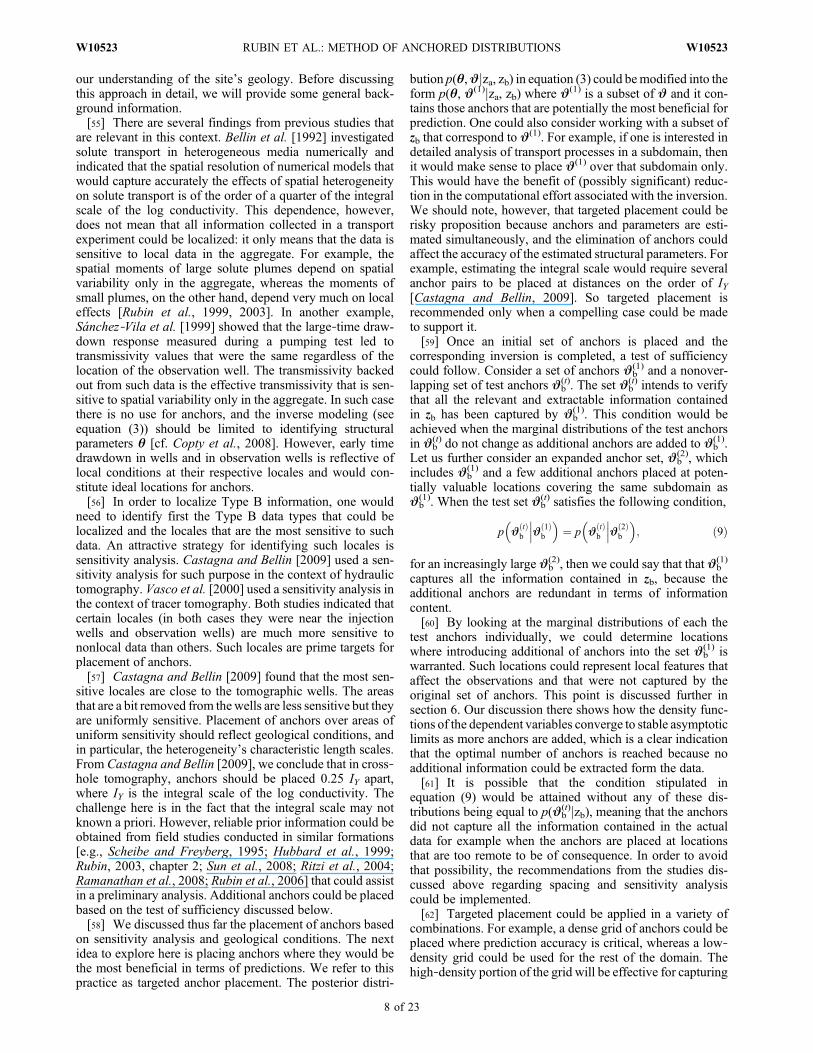
[74] Figure 2 is an aerial view of the aquifer with the lo-cations of the Type A and Type B data and with severalcombinations of anchors. The mean flow direction is parallelto the y axis (see Appendix A for additional information).

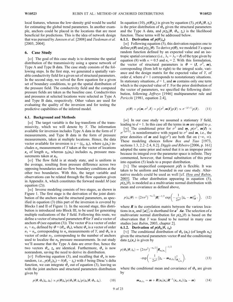
MAD was applied to each of these cases in order to evaluateusing different numbers and locations of the anchors.[75] Figure 3 shows the posterior distributions of the length

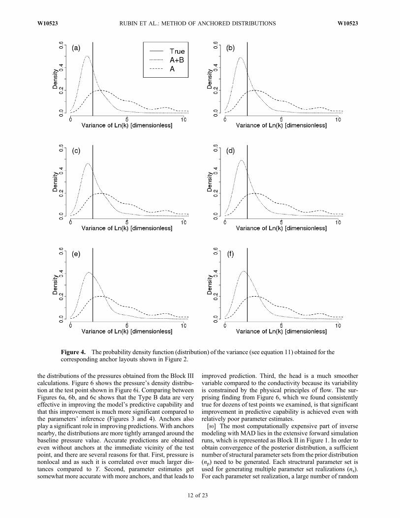
scale parameter I obtained using the various layouts of dataand anchors shown in Figure 2. We note that augmenting thedata base with Type B data has a favorable effect, leading todistributions that are narrower compared with those obtainedusing Type A data only. Adding anchors also has a favorableeffect. Figure 3f depicts the mode of the distribution just nextto the actual value of the scale. The posterior distribution isnot much of an improvement compared to the prior. The scaleis relatively large compared to the aquifer’s domain. Thedomain would need to be much larger than the scale in orderto be ergodic with respect to the scale.[76] Figure 4 shows the marginal distributions for the

variance s2. Here we note that the contribution of the Type B

Figure 2. Various layouts showing the locations of Type A data, Type B data, and anchors. Thenumber of anchors used in each configuration is as follows: (a) no anchors used; (b) 11 anchors;(c) 11 anchors; (d) 11 anchors; (e) 19 anchors; (f) 36 anchors.

RUBIN ET AL.: METHOD OF ANCHORED DISTRIBUTIONS W10523W10523

10 of 23

data is more significant compared to what we saw in Figure 3even when no use is made of anchors. We could also note thatthe mode of the distribution is getting somewhat closer to theactual value as the number of anchors increase, but theimprovement is minor. The variance is a statistic much easierto infer than the scale, because the scale is a compoundaggregate of length scales of the various geological units inthe aquifer [cf. Ritzi et al., 2004; Rubin et al., 2006; Sunet al., 2008].[77] For accurate prediction of processes (e.g., prediction

of pressures, in this case study), is it critical to be able toobtain accurate parameter estimates? This is an importantquestion because the goal of studies such as this is not theestimation of the geostatistical model parameters.Diggle andRibeiro [2006, p. 160] speculated that difficulties in esti-mating the parameters may not necessarily translate into poorestimates of the processes. This question is addressed below.

[78] Figure 5 evaluates the combined impact of measure-ments and anchors on a couple of transects along the aquifer.Two transects are examined. The transect on the left is sur-rounded by measurements and anchors. The other one issomewhat removed from the measurement locations, andrelies mostly on anchors as sources of local information. Bothtransects show tighter bounds as the data base is augmentedwith Type B data (Figure 5b) and with the addition of anchors(Figure 5c). The transect on the right shows only a minorimprovement as anchors are introduced due to the largerdistance from the measurement locations.[79] A different way to evaluate the quality of the inversion

results is to evaluate the improvement of the inferred model’spredictive capability for various combinations of data andanchors. This can be done through application of Block III(see Figure 1). We selected several test points throughout theaquifer’s domain and compared the baseline pressures with

Figure 3. The probability density function (distribution) of the scale (see equation (11)) obtained for thecorresponding anchor layouts shown in Figure 2.

RUBIN ET AL.: METHOD OF ANCHORED DISTRIBUTIONS W10523W10523

11 of 23

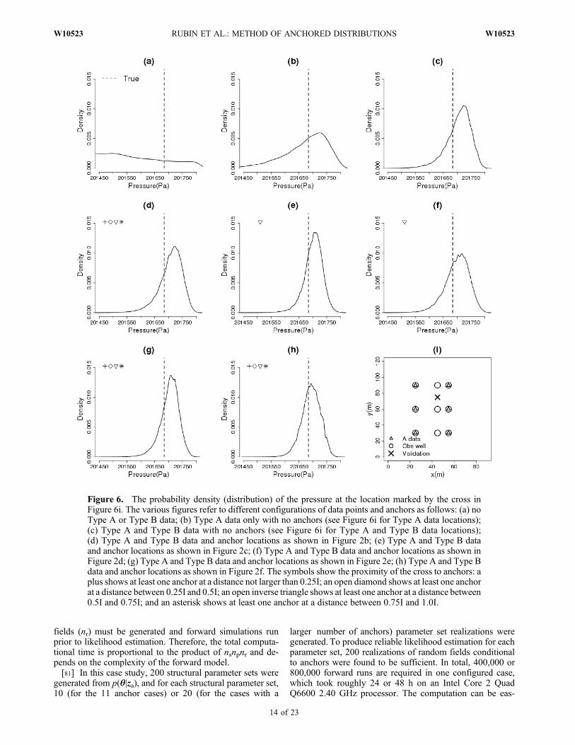
the distributions of the pressures obtained from the Block IIIcalculations. Figure 6 shows the pressure’s density distribu-tion at the test point shown in Figure 6i. Comparing betweenFigures 6a, 6b, and 6c shows that the Type B data are veryeffective in improving the model’s predictive capability andthat this improvement is much more significant compared tothe parameters’ inference (Figures 3 and 4). Anchors alsoplay a significant role in improving predictions. With anchorsnearby, the distributions are more tightly arranged around thebaseline pressure value. Accurate predictions are obtainedeven without anchors at the immediate vicinity of the testpoint, and there are several reasons for that. First, pressure isnonlocal and as such it is correlated over much larger dis-tances compared to Y. Second, parameter estimates getsomewhat more accurate with more anchors, and that leads to

improved prediction. Third, the head is a much smoothervariable compared to the conductivity because its variabilityis constrained by the physical principles of flow. The sur-prising finding from Figure 6, which we found consistentlytrue for dozens of test points we examined, is that significantimprovement in predictive capability is achieved even withrelatively poor parameter estimates.[80] The most computationally expensive part of inverse

modeling with MAD lies in the extensive forward simulationruns, which is represented as Block II in Figure 1. In order toobtain convergence of the posterior distribution, a sufficientnumber of structural parameter sets from the prior distribution(np) need to be generated. Each structrural parameter set isused for generating multiple parameter set realizations (ns).For each parameter set realization, a large number of random

Figure 4. The probability density function (distribution) of the variance (see equation 11) obtained for thecorresponding anchor layouts shown in Figure 2.

RUBIN ET AL.: METHOD OF ANCHORED DISTRIBUTIONS W10523W10523

12 of 23

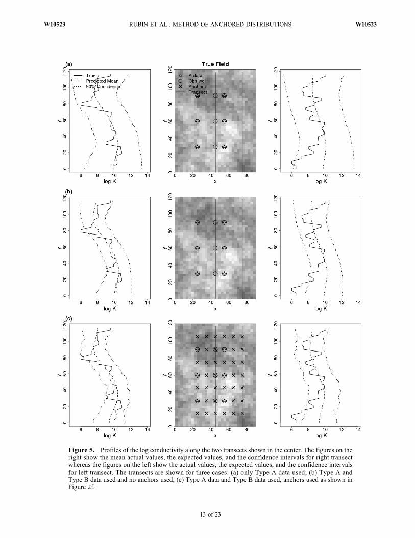
Figure 5. Profiles of the log conductivity along the two transects shown in the center. The figures on theright show the mean actual values, the expected values, and the confidence intervals for right transectwhereas the figures on the left show the actual values, the expected values, and the confidence intervalsfor left transect. The transects are shown for three cases: (a) only Type A data used; (b) Type A andType B data used and no anchors used; (c) Type A data and Type B data used, anchors used as shown inFigure 2f.

RUBIN ET AL.: METHOD OF ANCHORED DISTRIBUTIONS W10523W10523

13 of 23

fields (nr) must be generated and forward simulations runprior to likelihood estimation. Therefore, the total computa-tional time is proportional to the product of nsnpnr and de-pends on the complexity of the forward model.[81] In this case study, 200 structural parameter sets were

generated from p(q|za), and for each structural parameter set,10 (for the 11 anchor cases) or 20 (for the cases with a

larger number of anchors) parameter set realizations weregenerated. To produce reliable likelihood estimation for eachparameter set, 200 realizations of random fields conditionalto anchors were found to be sufficient. In total, 400,000 or800,000 forward runs are required in one configured case,which took roughly 24 or 48 h on an Intel Core 2 QuadQ6600 2.40 GHz processor. The computation can be eas-

Figure 6. The probability density (distribution) of the pressure at the location marked by the cross inFigure 6i. The various figures refer to different configurations of data points and anchors as follows: (a) noType A or Type B data; (b) Type A data only with no anchors (see Figure 6i for Type A data locations);(c) Type A and Type B data with no anchors (see Figure 6i for Type A and Type B data locations);(d) Type A and Type B data and anchor locations as shown in Figure 2b; (e) Type A and Type B dataand anchor locations as shown in Figure 2c; (f) Type A and Type B data and anchor locations as shown inFigure 2d; (g) Type A and Type B data and anchor locations as shown in Figure 2e; (h) Type A and Type Bdata and anchor locations as shown in Figure 2f. The symbols show the proximity of the cross to anchors: aplus shows at least one anchor at a distance not larger than 0.25I; an open diamond shows at least one anchorat a distance between 0.25I and 0.5I; an open inverse triangle shows at least one anchor at a distance between0.5I and 0.75I; and an asterisk shows at least one anchor at a distance between 0.75I and 1.0I.

RUBIN ET AL.: METHOD OF ANCHORED DISTRIBUTIONS W10523W10523

14 of 23

ily parallelized because the forward runs of Block II (seeFigure 1) on different parameter combinations can be con-ducted independently.

7. Updating With Multiple Data Sets

[82] Inverse modeling is a complex process of data accu-mulation and assimilation. Multiple data types and data setscould be acquired for the purpose of enhancing the qualityof the inversion. Most commonly, data sets are acquiredsequentially and at times over extended periods of time. Suchprocess of data acquisition necessitates repeated applicationsof the inverse modeling algorithm. Bayesian methods arevery efficient in this regard. Consider for example, a casewhere zb = (zb

(1), zb(2)), where zb

(1) and zb(2) are two subsets of data

collected at different times, and the set of anchors Jb = (Jb(1),

Jb(2)) corresponding to zb = (zb

(1), zb(2)). The two sets, Jb

(1) andJb(2), may be identical or may overlap to some extent

(meaning that a few anchors may appear in both sets). Withthis, the likelihood in equation (3), p(zbjq, J), can be modi-fied as follows,

p zbjq;Jð Þ ¼ p zð1Þb ; zð2Þb

���q;Ja;Jð1Þb ;Jð2Þ

b

� �

¼ p zð2Þb

���zð1Þb ; q;Ja;Jð1Þb ;Jð2Þ

b

� �p zð1Þb

���q;Ja;Jð1Þb ;Jð2Þ

b

� �

¼ p zð2Þb

���q;Ja;Jð1Þb ;Jð2Þ

b

� �p zð1Þb

���q;Ja;Jð1Þb ;Jð2Þ

b

� �:

ð16Þ

In the second line, zb(1) is removed from the list of conditioning

terms because its informational content is captured by Jb(1). If

zb(1) and zb

(2) do not overlap spatially (e.g., two pump testsconducted in two different and far‐apart subdomains), thenthe likelihood could be simplified further into the form,

p zb���q;J� �

¼ p zð2Þb

���q;Ja;Jð2Þb

� �p zð1Þb

���q;Ja;Jð1Þb

� �: ð17Þ

Updating the likelihood in MAD is performed using atwo‐step approach as follows. In the first step, when zb

(1) isthe only data set available, the likelihood is equal to p(zb

(1)jq,Ja, Jb

(1), Jb(2)) or p(zb

(1)jq, Ja, Jb(1)), depending on whether

equation (16) or (17) is used. Substituting these distributionsinto equation (3) leads to a posterior given Type A data andzb(1). The second step takes place when zb

(2) becomes available.In that case, the likelihood is given by the products givenin equation (16) or (17). This would require us to com-pute only the conditional distributions of zb

(2), because theconditional distribution of zb

(1) is already known from thefirst step. This procedure can be expanded to include anynumber of additional data sets, zb

(3), ..., zb(N), with each new

data set introduced being used to update the posterior distri-bution, without requiring recomputation of the previouslycomputed likelihood(s).[83] In contrast, the problem with optimization‐based

method (such as the pilot points method, see section 8) is thatoptimal results obtained based on zb

(1) cannot be used as astarting point for an update based on zb

(2). For example, in thecase of pilot points (see section 8), one could only speculatethat the optimized pilot points, obtained using initial set ofdata, could be used as a starting point for further updating.

And so, once zb(2) is acquired, the optimization‐based

parameter search must start anew.

8. MAD vis à vis Other Inversion Methods

[84] This section discusses the similarities and dissim-ilarities between MAD and several other inverse modelingapproaches for the purpose of adding perspective. We willidentify and discuss differences in the assumptions and con-cepts employed, and we will look at some results. This dis-cussion is not intended to be a comprehensive review, butrather to highlight a few points in order to clearly positionMAD vis à vis other methods.[85] Inverse modeling in hydrology may (or may not)

include elements of estimation and simulation. Estimationrefers to obtaining estimates for parameters of interest basedprimarily on statistical laws or considerations on one hand, oron meeting fitting criteria, on the other. Similarly, simulationrefers to generating a single or multiple realizations of theparameters based on statistical laws or one or more fittingcriteria. One can thus define two conceptual approaches, ordomains, to inverse modeling: one that is defined by statis-tical laws and one that is defined by fitting criteria. Theboundaries between these two domains are not sharp, but theyare useful in trying to map the terrain of inverse modeling:Inverse modeling can be defined based on how they arepositioned, in terms of their primary goals or products (withsome variations between authors) on the spectrum defined bythese two domains.[86] The methods of maximum likelihood (ML) and

maximum a posteriori (MAP) are positioned on the proba-bilistic side of the spectrum and they focus primarily onestimation. In MAP, for example, following the MAP con-cept, one gets a MAP estimate, whereas drawing samplesfrom the MAP distribution, if available, would amount tosimulation. The pilot point method is positioned on the fittingside of spectrum, with a focus on simulation because it isdefined by an objective function that is based on one or morefitting criteria, and because it produces some sort of condi-tional simulations. MAD is positioned on the probabilisticside of the spectrum, and it includes elements from bothestimation and simulation, as will be explained in our sub-sequent discussion.

8.1. MAD and Maximum Likelihood (ML)

[87] MAD and ML are both probabilistic methods. Thedifference between MAD and ML is that ML is focused onfinding an estimate of the unknown parameter, and is thus anestimation theory method, whereas MAD focuses on ob-taining the distribution of the unknown parameter, and is thusa Bayesian method. It can be shown that MAD is an exten-sion of the ML logic. For example, the ML approach ofKitanidis and Vomvoris [1983] can be related to MADthrough equation (3). ML focuses on the likelihood term inequation (3), namely, p(zb, zajq), and aims at estimating thevector q. Usually, a modeling assumption is madewith regardto this distribution and the parameters of the assumed dis-tribution comprise the vector q. The ML parameter esti-mates are those that maximize the model approximation ofp(zb, zajq), or in other words, the probability of observingthe data. The parameter vector q models the global trends ofthe target variable (e.g., through its moments), and it is not

RUBIN ET AL.: METHOD OF ANCHORED DISTRIBUTIONS W10523W10523

15 of 23

intended to capture local features, which is the role of theanchors in MAD. One could possibly add anchors into thelikelihood function, rewriting it in the form p(zb, zajq, J) andobtaining the ML estimates of both q and J. This would leadto a formulation of ML along the lines proposed by Carreraand Neuman [1986a, 1986b] and Riva et al. [2009]. Butincluding anchors in the likelihood function would notamount to transforming ML into MAD because ML derivessingle‐valued parameter estimates whereas MAD derivesparameter distributions.[88] One of the challenges facing ML is providing estima-

tion variances. Under some assumptions [Schweppe, 1973],ML can provide lower bounds for the estimation variances.These variances can be translated into statistical distributionsby assuming some sort of distribution: a Gaussian model isjustified asymptotically. The assumption of Gaussianity isreasonable and in many cases justified [cf. Woodbury andUlrych, 1993], but it cannot be guaranteed a priori. This isshown in Figure 3, where the distributions do not appear tobe Gaussian, but it appears that a Gaussian approximationcould work very well in this case. We will show later that itdoes not always work.

8.2. MAD and Maximum A Posteriori (MAP)

[89] MAP, similar to ML, is a probabilistic method thataims at obtaining parameter estimates [McLaughlin andTownley, 1996]. MAP derives parameter estimates but nottheir distributions. Consider the posterior distribution shownin equation (3), and let us do a couple of things: first, let usignore the anchors and second, let us replace the prior dis-tribution of the parameters with a prior distribution for za.This leaves us with the MAP distribution in the form:

p qjza; zbð Þ / p zajqð Þp zbjq; zað Þ: ð18Þ

MAP proceeds by assuming models for the distributionsappearing on the right‐hand side of equation (18). The MAPparameter estimates are those that maximize the modelapproximation of equation (18). In other words, the MAPparameter estimates are those that correspond to the mode ofthe parameter distribution.[90] The prior p(zajq) in MAP acts to regularize the solu-

tion by stabilizing it around the prior, but unlike the Pilot‐Point method (PPM), its weight is not manipulated to controlthe results: in MAP, the prior is a starting point, not a con-straint! We shall see below that the transformation of the priorterm into a regularization term, as done by PPM, has signif-icant consequences.[91] The likelihood function p(zbjq, za) is commonly taken

as p(eb) where eb = zb − M(~y). The error terms in p(eb) areusually assumed to be zero‐mean, uncorrelated and Gaussian[McLaughlin and Townley, 1996]. Similar assumptions couldbe made in ML. A modeling assumption is a required com-ponent of both ML and MAP because both seek parametervalues that are defined by a characteristic of the assumeddistributions (e.g., the mode in ML). In other words, both MLand MAP use parametric models. MAD, on the other hand,estimates the likelihood function and not its parameters, andhence can employ nonparametric likelihood functions. Theadvantage of employing nonparametric models is in theflexibility it offers in terms of model selection, but this ofcourse comes with a heavy computational price tag. Addi-

tional discussion on the differences between ML and MAP isprovided in the work of Kitanidis [1997a, 1997b].

8.3. MAD and the Pilot Point Method (PPM)

[92] In this section, we will highlight the differencesbetween PPM andMAD. PPMwas reported in several studies[e.g., Doherty et al., 2003; Kowalsky et al., 2004; Hernandezet al., 2006; Alcolea et al., 2006]. PPM is fundamentallydifferent fromML,MAP andMAD in that it is amodel‐fittingmethod and not a probabilistic method. We will show thatPPM’s goals are vastly different from the other methods, andwe will show how meeting these goals affect the results. Wewill also show that pilot points are not anchors: not only byname but also not in concept.[93] Let is start by summarizing how PPM works. Sche-

matically, it works like this (specific details may varybetween authors):[94] 1. Define a vector of structural parameters q using the

data za.[95] 2. Generate an unconditional realization of Y. The

generated field ~y0 is made conditional on za.[96] 3. Determine the number and locations of the pilot

points, and assign to them initial values y0. The initial set ofpilot point values y0 is taken from ~y0.[97] 4. Set an objective function. The objective function

intends to control the values assigned to the pilot points.Additional discussion of the objective function is providedbelow.[98] 5. Change the values of y0 to y following a determin-

istic optimization search procedure as follows. Starting withy0, the field ~y0 is conditioned deterministically on the pilotpoints, leading to the conditional field ~y. A numerical simu-lation of the process, relating the Type B data zb to ~y, is thenperformed. The results of this simulation are then comparedwith the measured zb values, and y is modified with thegoal of improving on the objective function. The processis repeated with the goal of reaching eventually a presetthreshold value for the objective function. The search is ter-minated once the threshold is crossed.[99] 6. The final product of this process is the field ~y0

conditioned on the set of pilot point values y that wereobtained from the optimization process.[100] Following this summary, we shall look at the fol-

lowing aspects of PPM: (1) The significance of PPM’s statedgoals, (2) the use of pilot points as fitting parameters, and (3)the implications of the optimization procedure. In doing so,we shall also highlight the differences between PPM and theother methods.[101] By following the procedure outlined above, PPM

attempts to achieve several goals [Cooley, 2000, and Cooleyand Hill, 2000]. The first goal is to maintain the frequencydistribution of the target variable in ~y similar to the distribu-tion observed by measurements of the target variable. Thesecond goal is to generate realizations of ~y that are equallylikely, and the third goal is to closely reproduce the obser-vations of the dependent variables zb.[102] Let us consider the first goal. This goal poses several

challenges because, first, the observed distributions of thetarget variable are either poorly defined or nonexistent tobegin with. However, for the sake of discussion, let us assumethat some data are available to construct a prior distributionfor Y from Type A data, p(yjza). If Type B data is available,

RUBIN ET AL.: METHOD OF ANCHORED DISTRIBUTIONS W10523W10523

16 of 23

it should be used as additional source of information, leadingto p(yjzb, za). These distributions could be different, and it isreasonable to expect that they will, because the Type B databrings additional information into consideration. And so weshould ask ourselves whether it is reasonable or helpful toconsider p(yjza) as a constraint. MAP andMAD recognize thesignificance of the prior, but they do not use it as a constraint:they use it as a starting point, because they recognize that itcould change if we have informative Type B data. Similarly,ML does not use p(yjza) as a constraint.[103] The second PPM goal [Cooley and Hill, 2000] is the

generation of equally likely realizations of the target vari-able field ~y. This goal is challenging on several counts. First,generating a realization is a Bayesian concept. Within clas-sical statistics we have the concept of generating conditionalrealizations of estimates, which can be obtained by somehowperturbing the data. PPM is not a Bayesian concept nor anestimation method, so it is unclear what the PPM realizationsrepresent. Second, there is a question of semantics here: inorder to qualify multiple realizations as equally likely, oneneeds to have a statistical model to quantify that likelihood inthe first place, which PPM does not have. So perhaps a moreaccurate adjective to use instead of “equally likely” would be“equally drawn.” Third, even if one assumes that PPM cangenerate equally likely realizations, the advantage of workingwith such realizations is questionable, because for predictionone would want to consider more likely and less likely rea-lizations, or in short, random sampling. Random sampling isthe key for sampling the complete probability space withoutbias. It is a fundamental tenet of statistics that samples mustbe drawn at random [Mugunthan and Shoemaker, 2006]in order to prevent bias. Equally likely realizations do notamount to random sampling, as shown in the next para-graph. MAD, in contrast, produces plausible realizations, withvarious degrees of plausibility, as measured by probability.[104] Let us be more specific with regard to the third point

of the last paragraph. PPM considers only realizations thatcross a preset threshold value defined for the objectivefunction. That means that realizations that do not cross thethreshold will not be admitted into the pool of realizations.But the rejected realizations may be defined by nonzeroprobability, and hence should not be eliminated from consid-eration. Surprisingly, it is not only poor‐performing (“poor”from the PPM objective function sense) realizations thatare rejected by PPM, but also the superior realizations arerejected, because the PPM search algorithm stops once thepreset threshold is crossed, and no efforts are made to fur-ther improve them. We can conclude then that PPM under‐samples the probability space, and is potentially biased. Thebias effect due to optimization was noted in Mugunthan andShoemaker [2006, p. W10428] where a comment is madeon “…bias introduced during optimization because of over‐sampling of high goodness‐of‐fit regions of the parameter…”These effects may be small or large, we cannot say. For acredible application, PPM applications must show that thiseffect is small.[105] An important implication of the biased sampling is

that PPM cannot assign probabilities to realizations. Conse-quently, users cannot assign probabilities to events that aremodeled based on the PPM realizations. In MAD, on theother hand, no optimization is used and no threshold cri-teria are set, thus avoiding all these issues altogether. The

probability space is sampled exhaustively and withoutbias, and realizations can be associated with probabilitiesusing the posterior distributions or by looking at histogramsof events.[106] Let us now take a look at the role of the pilot points in

achieving the PPM third goal, which is the reproduction of theobservations. PPM uses pilot points as fitting parameters.PPM uses many pilot points for that, and in fact it encouragesthe user to add as many pilot points as one would need[Doherty, 2003]. This aspect of PPM underlies its need to usethe plausibility term (synonymous with the more often usedregularization term) discussed in Step 4 of the algorithm. Theplausibility term is used to control the problem of using anumber of fitting parameters (the pilot points) that can farexceed the number of observations. Tikhonov and Arsenin[1977] showed theoretically that it is possible for a modelto fit observations exactly when the number of parameters isequal to the number of data, and that additional parametersrender the problem singular unless regularization is applied.This situation applies to PPM, and was confirmed in a studyof PPMbyAlcolea et al. [2006, p. 1679] who commented thatover‐parameterization (in the form of a large number of pilotpoints) “…leads to instability of the optimization problem”and that “…instability implies…large values of some modelparameters due to unbounded fluctuations … large jumps inthe value of hydraulic properties…” etc. This instability isbrought under control in PPM by the regularization term[which is referred to as the plausibility term in Alcolea et al.,2006]. The weight assigned to the plausibility term can bemade arbitrarily large (or small) depending on the magnitudeif the instability. That effect, although beneficial from theinstability perspective, is the root cause of PPM’s biasedsampling because it controls the extent of censoring (fromboth the “bad” and “good” realizations sides, as discussedearlier). It should also be noted that “…the degree of datareproduction is a poor indicator of the accuracy of estimates”[Kitanidis, 2007].[107] In additional to creating instability, pilot points can

lead to artifacts in the generated fields. Because in PPM theintroduction of additional pilot points is the only PPMmechanism for improvingmodel performance and addressingneglected elements (such as three‐dimensional flow,unsteady flow, recharge and leakage, geological discontinu-ity and such), it could lead to the appearance of artificialfeatures in the target variable field realizations [see Cooley,2000, p. 1162]. Alcolea et al. [2006, p.1679], confirmed theexistence of this effect and indicated that it could be con-trolled by regularization, but it is unclear how and to whatextent. Kitanidis [2007] also confirmed the existence of thiseffect when he noted that “By over‐weighting the datareproduction penalty, the data are reproduced more closelyandmore details appear in the image that is estimated from theoptimization but the image is also more affected by spuriousfeatures.” Studies such as Hernandez et al. [2006] suggestthat the artifact issue can be brought under control, but it isunclear what constitutes an artifact (except after it shows up)and how this aspect of the simulation can be managed. Tosummarize, the plausibility term, in addition to controllinginstability, is also used for reducing artifacts. But in theabsence of any indication to the contrary, one can onlyspeculate on how efficient it is in doing so.

RUBIN ET AL.: METHOD OF ANCHORED DISTRIBUTIONS W10523W10523

17 of 23

[108] The fundamental difference between PPM and MADin this regard is thatMAD is a Bayesianmethodwhereas PPMis a model‐fitting method. Specifically, anchors are not fittingparameters: they are devices for reducing data into a suit-ably convenient form. PPM attempts to fit measurementsby adding pilot points and tweaking their assigned values,whereas MAD does not fit anything: it is built around esti-mating statistical distribution of the differences between ob-servations and model predictions. MAD can use parametersto model distributions, but it does not adjust point estimates.[109] The likelihood function inMAD is the only subject of

estimation. Estimating the likelihood function in MAD isunlike the fitting exercise of PPM because of the number ofdata points involved. In PPM the number of data points islimited to the number of measurements, whereas in MAD thenumber of data points corresponds to the number of differ-ences between measurements and predictions, which can beset arbitrarily high (it depends on the number of Monte Carlorealizations generated for the purpose of estimating the like-lihood function). For example, consider the case of N mea-surements. PPM attempts to fit the N measurements with anumber of pilot points that can far exceedN, whereas inMADthe number of data points is on the order of N × 106 or more.Theoretically, there is no limit on the number of realizationsthat could be generated, and hence stability is not an issue inMAD.[110] The issue of stability is demonstrated in Figure 6.

Figure 6 shows the marginal distribution of the pressure at avalidation point (this is a point not used for inversion, but fortesting the quality of the predictions). The pressure distribu-tion is shown here for different numbers of anchors. Thedistribution does not show any sign of instability as thenumber of anchors increases. Similar stability was observedfor dozens of points spread all over the simulated domain.Figure 6 demonstrates that MAD does not have a stabilityproblem, despite the fact that it does not use any regulariza-tion term. It also highlights the issue of anchor placement (seesection 5), the point being that the convergence of the sta-tistical distributions of the target variables provides an indi-cation that the number of anchors used reached a satisfactorylevel in terms of the ability to extract information form thedata. Such a measure of sufficiency is not available withPPM.

8.4. Comparison With Hernandez et al. [2006]

[111] This section includes a brief comparison of MADwith the PPM case study presented by Hernandez et al.[2006], subsequently referred to as H06. The case studyfocuses on a rectangular flow domain with spatially variableY = ln(conductivity). The spatial variability is modeled usinga stationary mean and an exponential spatial covariance withvariance of Y, sY

2, equal to 4, and an integral scale equal to 1.The hydraulic head gradient was defined by a head differenceof 10 length units. For both the head and Y, measurementerrors were added to the data, defined by a unit variance. Weimplemented the same models in our case study. We did nothave access to the baseline Y field of H06, and we generatedour own baseline field using the same spatial variabilitymodel.[112] As discussed earlier, there are fundamental differ-

ences between MAD and PPM and we shall not repeat them

here. In this section we shall focus on specific details relatedto the implementation of MAD and PPM to this case studyand on some results. The first difference between MAD andH06 is with regard to estimating the parameters of the spatialvariability model. H06 provides estimates for the parametersbased on alternative criteria of optimality, whereas MADconsiders the statistical parameters as random variables andderives their distributions.[113] The second difference concerns the statistical model

that was employed for modeling the joint distribution of theheads and Y. H06 assumed the heads to be spatially uncor-related. Their model amounts to assuming that the heads aredeterministic variables subject to uncertainty due to spatiallyuncorrelated errors (which is the structure often assumedfor measurement error). This assumption is not in line withthe approach employed by H06 for modeling of Y, whichassumed Y to be a spatially correlated space random function.H06 also assumed the heads to be uncorrelated with Y,whereas Y was assumed to be normally distributed and spa-tially correlated. These assumptions are not in line withmultiple studies and observations that showed the heads to bespatially correlated and cross‐correlated with Y, and further-more, to be normally distributed only for sY

2 smaller than 1[Rubin, 2003]. This statistical model was employed in otherstudies as well [cf. Kowalsky et al., 2004]. Regardless ofwhether this model is justified or not, the point we want tomake is that PPM assumptions are made which may besimplified or restrictive. MAD, in contrast, does not requiremaking any assumption in this regard, and it derives a non-parametric posterior distribution.[114] We chose to demonstrate the differences with two

sets of results. The first set of results focuses on the hydraulicheads, and the second set focuses on the geostatisticalparameters. Figure 7 shows the actual and expected values ofthe hydraulic head along the centerline of the flow domain.We also show the 95% confidence intervals obtained withMAD as well as those identified by H06 and given in theirFigure 5. Our 95% confidence intervals are taken directlyfrom the head distribution (see Figure 8) whereas H06 ob-tained theirs by computing the variance of the head throughthe ensemble of realizations and assuming a Gaussian dis-tribution. Comparison of confidence intervals shows ourconfidence intervals to be somewhat larger than those pre-dicted by H06. As discussed earlier, PPM censors suboptimalas well as above‐threshold optimal realizations, which leadsto underestimation of the confidence intervals and explainsthis difference. H06 upper confidence interval near the leftboundary allows the head to vary above the head at theboundary, and similarly, the head is allowed to vary below thelower bound set by the right boundary. This is an outcome ofthe assumption of Gaussianity. In MAD, however, the upperand lower bounds of the distributions next to the boundariesare bounded correctly, because the distribution is derived, notpostulated.[115] Figure 8 shows the head distributions at different

locations along the transect shown in Figure 7. The dis-tributions are shown on q‐q plots, so that we could evaluatetheir departure from Gaussianity. We note that the head dis-tributions are non‐Gaussian throughout the flow domain.They are strongly skewed next to the boundaries becauseof the constraints imposed by the nearby boundaries. Thedeparture from Gaussianity is much less pronounced around

RUBIN ET AL.: METHOD OF ANCHORED DISTRIBUTIONS W10523W10523

18 of 23

the center of the flow domain (Figure 8c), but the departurefrom Gaussianity is still pronounced at the tails. H06, on theother hand, assumes the heads to be Gaussian throughoutthe transect. One consequence of that assumption is that headsare allowed to be larger than 10 and smaller than zero next tothe upper and lower boundaries, respectively. As noted ear-lier, MAD does not assume posterior distributions, but ratherinfers them, and a consequence of that is the flexibility toobtain a variety of distributions, and a better compliance withthe underlying physics.[116] Our next set of results deals with estimates of the

geostatistical parameters, whichMADprovides in the form ofstatistical distributions. Figure 9a shows the probabilitydensity functions obtained by MAD for three different sets ofdata and error levels. In all cases the distributions are well‐aligned with the theoretical the actual value, which is around1 unit length. H06 deals with this parameter in their Figure 14.They do not provide distributions. Instead, they attempt toidentify an optimal value by analyzing various performancecriteria for a wide range of parameter values. Theoretically,these criteria should peak at the vicinity of the actual values.Of the five evaluation criteria tested in Figure 14 of H06, nonepeaked at around 1, but instead peaked at around zero.[117] Figure 9(b) provides our results for the variance. All

cases we analyzed show well‐defined peaks somewherebetween 4 and 5 (with the higher values corresponding to thecase with large measurement error on the heads). Results inH06 for this parameter are provided in their Figures 13 and16. The evaluation criteria they used did not peak at the actualvalues. A few criteria show preference toward high values,but without displaying a well‐defined peak. The variousevaluation criteria in H06 are not consistent in the trends theydisplay. For example, in Figure 13 of H06 one the evaluationcriteria identified the variance at around 0.5 whereas theothers seem to prefer 6. This leaves unclear which criteriashould be selected a priori as the most reliable. We speculatethat this insensitivity or underperformance of the evaluationcriteria in H06 could be related (1) to the elimination of the

high‐probability and low‐probability events due to the use ofoptimality criteria as discussed in section 8.3 and (2) to theuse of multiple fitting parameters, in the form of pilot points,which masks the actual spatial structure by introducing arti-facts. This possibility was alluded to in the works of Cooley[2000] and Cooley and Hill [2000].

9. Summary

[118] We presented a Bayesian method for inversemodeling of spatially variable fields, called the method ofanchored distributions (MAD). This work expands in someparts on work done by Z. Zhang and Y. Rubin (unpublishedmanuscript, 2008). MAD is general in the sense that it is notlimited to particular data type or types or to any particularmodels. MAD is built around two new elements. The firstelement is a concept called anchored distributions and thesecond is a data classification scheme. On the basis of thesetwo concepts, various types of data can be combined, orassimilated, systematically into an improved image of therandom field.[119] MAD’s basic approach is to model the spatially

variable fields as random fields. In MAD, the random fieldis modeled through a combination of structural parametersand anchors. Structural parameters capture the global trendsand statistical characteristics of the random fields, whereasanchored distributions capture the local effects. Anchoreddistributions are statistical devices that extract informationfrom data that is directly or indirectly and locally or non-locally related to the target variable. The information iscaptured in the form of statistical distributions of the targetvariable.[120] Data used for inversion is classified by the way it

is related to the target variable. We distinguish betweendata that is local and directly related to the target variables(Type A) and to data that is nonlocal and indirectly related tothe target variables (Type B). Both types of data are rep-resented using anchors. In the case of Type A data, anchors

Figure 7. The hydraulic head along the center line of the flow domain. Reference denotes the actual head.The predicted mean is obtained using MAD based on the posterior distributions of the parameters and an-chors. The 95% confidence intervals shown are those obtained by MAD and by Hernandez et al. [2006],denoted here by H06.

RUBIN ET AL.: METHOD OF ANCHORED DISTRIBUTIONS W10523W10523

19 of 23

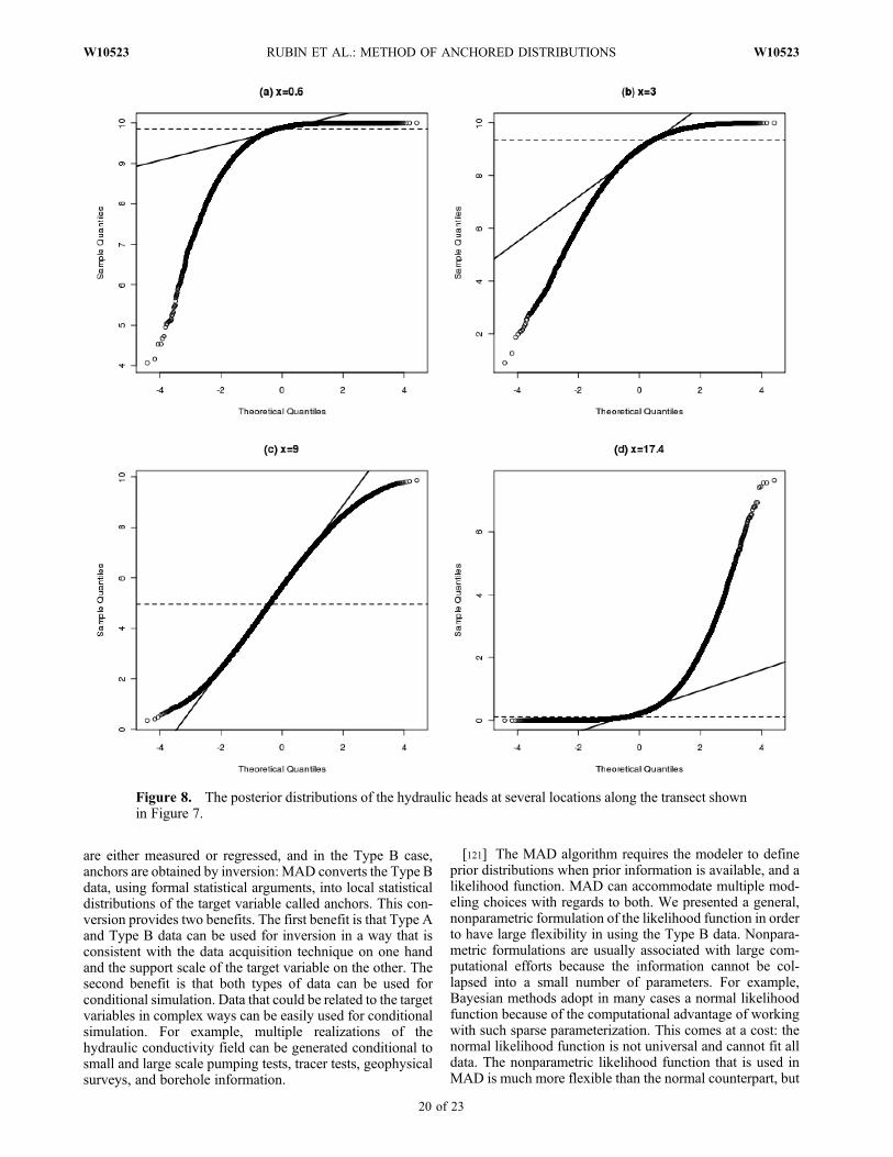
are either measured or regressed, and in the Type B case,anchors are obtained by inversion: MAD converts the Type Bdata, using formal statistical arguments, into local statisticaldistributions of the target variable called anchors. This con-version provides two benefits. The first benefit is that Type Aand Type B data can be used for inversion in a way that isconsistent with the data acquisition technique on one handand the support scale of the target variable on the other. Thesecond benefit is that both types of data can be used forconditional simulation. Data that could be related to the targetvariables in complex ways can be easily used for conditionalsimulation. For example, multiple realizations of thehydraulic conductivity field can be generated conditional tosmall and large scale pumping tests, tracer tests, geophysicalsurveys, and borehole information.

[121] The MAD algorithm requires the modeler to defineprior distributions when prior information is available, and alikelihood function. MAD can accommodate multiple mod-eling choices with regards to both. We presented a general,nonparametric formulation of the likelihood function in orderto have large flexibility in using the Type B data. Nonpara-metric formulations are usually associated with large com-putational efforts because the information cannot be col-lapsed into a small number of parameters. For example,Bayesian methods adopt in many cases a normal likelihoodfunction because of the computational advantage of workingwith such sparse parameterization. This comes at a cost: thenormal likelihood function is not universal and cannot fit alldata. The nonparametric likelihood function that is used inMAD is much more flexible than the normal counterpart, but

Figure 8. The posterior distributions of the hydraulic heads at several locations along the transect shownin Figure 7.

RUBIN ET AL.: METHOD OF ANCHORED DISTRIBUTIONS W10523W10523

20 of 23

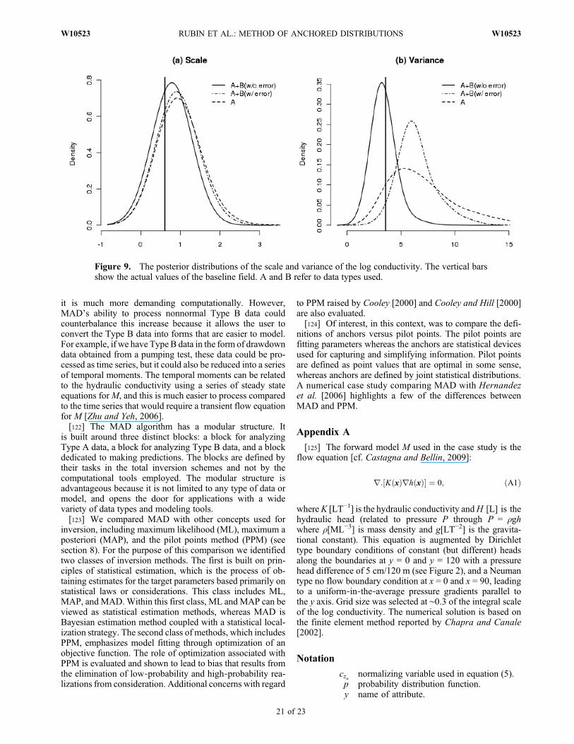
it is much more demanding computationally. However,MAD’s ability to process nonnormal Type B data couldcounterbalance this increase because it allows the user toconvert the Type B data into forms that are easier to model.For example, if we have Type B data in the form of drawdowndata obtained from a pumping test, these data could be pro-cessed as time series, but it could also be reduced into a seriesof temporal moments. The temporal moments can be relatedto the hydraulic conductivity using a series of steady stateequations forM, and this is much easier to process comparedto the time series that would require a transient flow equationfor M [Zhu and Yeh, 2006].[122] The MAD algorithm has a modular structure. It

is built around three distinct blocks: a block for analyzingType A data, a block for analyzing Type B data, and a blockdedicated to making predictions. The blocks are defined bytheir tasks in the total inversion schemes and not by thecomputational tools employed. The modular structure isadvantageous because it is not limited to any type of data ormodel, and opens the door for applications with a widevariety of data types and modeling tools.[123] We compared MAD with other concepts used for

inversion, including maximum likelihood (ML), maximum aposteriori (MAP), and the pilot points method (PPM) (seesection 8). For the purpose of this comparison we identifiedtwo classes of inversion methods. The first is built on prin-ciples of statistical estimation, which is the process of ob-taining estimates for the target parameters based primarily onstatistical laws or considerations. This class includes ML,MAP, and MAD.Within this first class, ML andMAP can beviewed as statistical estimation methods, whereas MAD isBayesian estimation method coupled with a statistical local-ization strategy. The second class of methods, which includesPPM, emphasizes model fitting through optimization of anobjective function. The role of optimization associated withPPM is evaluated and shown to lead to bias that results fromthe elimination of low‐probability and high‐probability rea-lizations from consideration. Additional concerns with regard

to PPM raised by Cooley [2000] and Cooley and Hill [2000]are also evaluated.[124] Of interest, in this context, was to compare the defi-

nitions of anchors versus pilot points. The pilot points arefitting parameters whereas the anchors are statistical devicesused for capturing and simplifying information. Pilot pointsare defined as point values that are optimal in some sense,whereas anchors are defined by joint statistical distributions.A numerical case study comparing MAD with Hernandezet al. [2006] highlights a few of the differences betweenMAD and PPM.

Appendix A

[125] The forward model M used in the case study is theflow equation [cf. Castagna and Bellin, 2009]:

r: K xð Þrh xð Þ½ � ¼ 0; ðA1Þ

whereK [LT−1] is the hydraulic conductivity andH [L] is thehydraulic head (related to pressure P through P = rghwhere r[ML−3] is mass density and g[LT−2] is the gravita-tional constant). This equation is augmented by Dirichlettype boundary conditions of constant (but different) headsalong the boundaries at y = 0 and y = 120 with a pressurehead difference of 5 cm/120 m (see Figure 2), and a Neumantype no flow boundary condition at x = 0 and x = 90, leadingto a uniform‐in‐the‐average pressure gradients parallel tothe y axis. Grid size was selected at ∼0.3 of the integral scaleof the log conductivity. The numerical solution is based onthe finite element method reported by Chapra and Canale[2002].

Notation

cza normalizing variable used in equation (5).p probability distribution function.y name of attribute.

Figure 9. The posterior distributions of the scale and variance of the log conductivity. The vertical barsshow the actual values of the baseline field. A and B refer to data types used.

RUBIN ET AL.: METHOD OF ANCHORED DISTRIBUTIONS W10523W10523

21 of 23

Y the SRF (space random function) of int-erest, for example the log conductivity.

~y a realization of the Y field.q vector of structural parameters describing t-

he spatial variability of Y.J = (Ja, Jb) vector of anchors corresponding to both

Type A and Type B data. The subscripts“a” and “b” refer to Type A data and TypeB data, respectively.

na number of Type A data.nb number of Type B data.

z = (za, zb) vector of Type A and Type B data of lengthna + nb.

~zb a realization of the zb field.x generic coordinate.

(xa, xb) vector of data locations. The vector xa de-notes the coordinates of za, etc.

x# = (x#a, x#b

) vector of anchor locations. The vector x#adenotes locations of anchors related to TypeA data. x#a and xa are identical.

M amodel, numerical or analytical, relating~y to~zb. For example, it could represent a flowmodel. When we have more than one typeof data in ~zb, then M would be a collectivename for all relevant models. Alternatively,Mi, i = 1, ..,N is used to denotemultiplemod-els.

e model error, composed of the two error vec-tors mentioned below.

ea error associated with Type A anchors.eb error associated with Type B anchors and

structural parameters

Notations: boldface type denotes vectors or fields.Superscript: when in parenthesis, denotes subset, e.g., J(1) isa subset of J.Subscripts: when a running index is used, denote the com-ponents of a vector. Otherwise denote name of a relatedvariable or data type.Notation for statistical distributions: p(..) is used to denotestatistical distributions. Different statistical distributions aredenoted by the name of the variables in parenthesis: p(q)and p(J) denote two different statistical distributions, notthe same statistical distribution estimated at different points.

[126] Acknowledgments. The authors wish to thank Peter Kitanidisfor stimulating discussions on this paper. This study has been funded bythe U. S. DOE Office of Biological and Environmental Research, Environ-mental Remediation Science Program (ERSP), through DOE‐ERSP grantDE‐FG02‐06ER06‐16 as part of Hanford 300 Area Integrated FieldResearch Challenge Project. This research used resources of the NationalEnergy Research Scientific Computing Center, which is supported bythe Office of Science of the U. S. Department of Energy under contractDE‐AC02‐05CH11231.

ReferencesAbramowitz, M., and I. A. Stegun (1965), Handbook of Mathematical

Functions, Dover, New York.Alcolea, A., J. Carrera, and A. Medina (2006), Pilot points method incor-

porating prior information for solving the groundwater flow inverseproblem, Adv. Water Resour., 29, 1678–1689.

Bellin, A., and Y. Rubin (2004), On the use of peak concentration arrivaltimes for the inference of hydrogeologic parameters, Water Resour. Res.,40, W07401, doi:10.1029/2003WR002179.

Bellin, A., P. Salandin, and A. Rinaldo (1992), Simulation of dispersion inheterogeneous porous formations: Statistics, first‐order theories, conver-

gence of computations, Water Resour. Res., 28(9), 2211–2227,doi:10.1029/92WR00578.

Box, G. E. P., and G. C. Tiao (1973), Bayesian Inference in StatisticalAnalysis, Addison‐Wesley, Reading, Mass.

Carrera, J., and S. P. Neuman (1986a), Estimation of aquifer parametersunder transient and steady state conditions: 1. Maximum likelihoodmethod incorporating prior information, Water Resour. Res., 22(2),199–210, doi:10.1029/WR022i002p00199.

Carrera, J., and S. P. Neuman (1986b), Estimation of aquifer parametersunder transient and steady state conditions: 2. Uniqueness, stability,and solution algorithms, Water Resour. Res., 22(2), 211–227.

Castagna, M., and A. Bellin (2009), A Bayesian approach for inversion ofhydraulic tomographic data, Water Resour. Res., 45, W04410,doi:10.1029/2008WR007078.

Chapra, S. C., and R. P. Canale (2002), Numerical Methods for Engineers,4th ed., McGraw‐Hill.

Copty, N. K., P. Trinchero, X. Sanchez‐Vila, M. S. Sarioglu, and A. N.Findikakis (2008), Influence of heterogeneity on the interpretation ofpumping test data in leaky aquifers, Water Resour. Res., 44, W11419,doi:10.1029/2008WR007120.

Cooley, R. L. (2000), An analysis of the pilot point methodology forautomated calibration of an ensemble of conditionally simulated trans-missivity fields, Water Resour. Res., 36(4), 1159–1163, doi:10.1029/2000WR900008.

Cooley, R. L., and M. C. Hill (2000), Comment on Ramarao et al. [1995]and LaVenue et al. [1995], Water Resour. Res., 36(9), 2795–2797,doi:10.1029/2000WR900174.

Dagan, G. (1985), Stochastic modeling of groundwater flow by uncondi-tional and conditional probabilities: The inverse problem, Water Resour.Res., 21(1), 65–72.

Dai, Z., R. W. Ritzi, C. Huang, Y. Rubin, and D. F. Dominic (2004), Trans-port in heterogeneous sediments with multimodal conductivity and hier-archical organization across scales, J. Hydrol., 294(1–3), 68–86.

Diggle, P. J., and P. J. Ribeiro (2006), Model‐Based Geostatistics, SpringerSeries in Statistics, Springer, New York.

Doherty, J. (2003), Groundwater model calibration using pilot points andregularization, Ground Water, 41(2), 170–177.

Ezzedine, S., Y. Rubin, and J. Chen (1999), Hydrogeological geophys-ical Bayesian method for subsurface site characterization: Theory andapplication to the LLNL Superfund Site, Water Resour. Res, 35(9),2671–2683.

Fuentes, M., and A. E. Raftery (2005), Model evaluation and spatial inter-polation by Bayesian combination of observations with outputs fromnumerical models, Biometrics, 61, 36–45.

Hayfield, T., and J. S. Racine (2008), P: Nonparametric econometrics: Thenp package, J. Stat. Software, 27(5), 1–32.

Hernandez, A. F., S. P. Neuman, A. Guadagnini, and J. Carrera (2006),Inverse stochastic moment analysis of steady state flow in randomly het-erogeneous media, Water Resour. Res., 42, W05425, doi:10.1029/2005WR004449.

Hoeksema, R. J., and P. K. Kitanidis (1984), An application of the geo-statistical approach to the inverse problem in two‐dimensional ground-water modeling, Water Resour. Res., 20(7), 1003–1020, doi:10.1029/WR020i007p01003.

Hoeting, J. A., D. MADigan, A. E. Raftery, and C. T. Volinsky (1999),Bayesian model averaging: A tutorial, Stat. Sci., 14(4), 382–417.

Hou, Z., and Y. Rubin (2005), On minimum relative entropy concepts andprior compatibility issues in vadose zone inverse and forward modeling,Water Resour. Res., 41(12), W12425, doi:10.1029/2005WR004082.

Hou, Z., Y. Rubin, G. M. Hoversten, D. Vasco, and J. Chen (2006), reser-voir parameter identification using minimum relative entropy basedBayesian inversion of seismic AVA and marine CSEM data, Geophysics,71(6), O77–O88.

Hoversten, G. M., F. Cassassuce, E. Gasperikova, G. A. Newman, Y. Rubin,Z. Hou, and D. Vasco (2006), Direct reservoir parameter estimation usingjoint inversion of marine seismic AVA & CSEM data, Geophysics, 71(3),C1–C13.

Hubbard, S., Y. Rubin, and E. Majer (1999), Spatial correlation structureestimation using geophysical and hydrogeological data, Water Resour.Res., 35(6), 1809–1825, doi:10.1029/1999WR900040.

Janssen, G. M. C. M., J. R. Valstar, and S. E. A. T. M. van der Zee (2008),Measurement network design including travel time determinations tominimize model prediction uncertainty, Water Resour. Res., 44,W02405, doi:10.1029/2006WR005462.

Jeffreys, H. (1946), An invariant form for the prior probability in estimationproblems, Proc. R. Soc. London, A186, 453–461.

RUBIN ET AL.: METHOD OF ANCHORED DISTRIBUTIONS W10523W10523

22 of 23

Kass, R. E., and L. Wasserman (1996), The selection of prior distributionsby formal rules, J. Am. Stat. Assoc., 91(435), 1343–1370.

Kitanidis, P. K. (1986), Parameter uncertainty in estimation of spatialfunctions: Bayesian analysis, Water Resour. Res., 22(4), 499–507,doi:10.1029/WR022i004p00499.

Kitanidis, P. K. (1991), Orthonormal residuals in geostatistics: Model crit-icism and parameter estimation, Math. Geol., 23(5), 741–758.

Kitanidis, P. K. (1995), Quasi‐linear geostatistical theory for inversing,Water Resour. Res., 31(10), 2411–2419, doi:10.1029/95WR01945.

Kitanidis, P. K. (1997a), Introduction to Geostatistics: Applications inHydrogeology, Cambridge Univ. Press., New York.

Kitanidis, P. K. (1997b), Comment on “A reassessment of the groundwaterinverse problems” by D. McLaughlin and L.R. Townley, Water Resour.Res., 33(9), 2199–2202, doi:10.1029/97WR00998.

Kitanidis, P. K. (2007), On stochastic inverse modeling, in SubsurfaceHydrology Data Integration for Properties and Processes, edited byD. W. Hyndman, F. D. Day Lewis and K. Singha, pp. 19–30, AGU,Washington, D. C.

Kitanidis, P. K., and E. G. Vomvoris (1983), A geostatistical approach tothe inverse problem in groundwater modeling (steady state) and one‐dimensional simulations, Water Resour. Res., 19(3), 677–690,doi:10.1029/WR019i003p00677.

Kowalsky, M. B., S. Finsterle, and Y. Rubin (2004), Estimating flowparameter distributions using ground‐penetrating radar and hydrologicalmeasurements during transient flow in the vadose zone, Adv. WaterResour., 27, 583–599.

Matérn, B. (1986), Spatial Variation, second ed., Springer, Berlin,Germany.

Mavko, G., T. Mukerji, and J. Dvorkin (1998), The Rock PhysicsHandbook, Cambridge Univ. Press, New York.

Michalak, A. M., and P. K. Kitanidis (2003), A method for enforcingparameter nonnegativity in Bayesian inverse problems with an applicationto contaminant source identification, Water Resour. Res., 39(2), 1033,doi:10.1029/2002WR001480.

Mugunthan, P., and C. A. Shoemaker (2006), Assessing the impacts ofparameter uncertainty for computationally expensive groundwater models,Water Resour. Res., 42, W10428, doi:10.1029/2005WR004640.

Neuman, S. P. (2003), Maximum likelihood Bayesian averaging of alterna-tive conceptual‐mathematical models, Stoch. Environ. Res. Risk Assess.,17(5), 291–305, doi:10.1007/s00477-003-0151-7.

Newton, M. A., and A. E. Raftery (1994), Approximate Bayesian inferencewith the weighted likelihood bootstrap, J. Roy. Stat. Soc., Ser. B, 56(1),3–48.

Nowak, W., F. P. J. de Barros, and Y. Rubin (2010), Bayesian geostatisticaldesign: Task‐driven optimal site investigation when the geostatisticalmodel is uncertain, Water Resour. Res., 46, W03535, doi:10.1029/2009WR008312.

Pericchi, L. R. (1981), A Bayesian approach to transformation to normality,Biometrika, 68(1), 35–43.

Poeter, E. P., and M. C. Hill (1997), Inverse models: A necessary next stepin ground‐water models, Ground Water, 35(2).

R Development Core Team (2007), R: A Language and Environment forStatistical Computing, R Foundation for Statistical Computing, Vienna,Austria.

Ramanathan, R., R. W. Ritzi, and C.C. Huang (2008), Linking hierarchicalstratal architecture to plume spreading in a Lagrangian‐based transportmodel, Water Resour. Res., 44, W04503, doi:10.1029/2007WR006282.

Ritzi, R. W., Z. Dai, D. F. Dominic, and Y. Rubin (2004), Spatial correla-tion of permeability in cross‐stratified sediment with hierarchical archi-tecture, Water Resour. Res., 40, W03513, doi:10.1029/2003WR002420.

Riva, M., A. Guadagnini, S. P. Neuman, E. B. Janetti, and B. Malama(2009), Inverse analysis of stochastic moment equations for transientflow in randomly heterogeneous media, Adv. Water Resour., 32,1495–1507.

Rubin, Y. (1995), Flow and transport in bimodal heterogeneous formation,Water Resour. Res., 31(10), 2461–2468, doi:10.1029/95WR01953.

Rubin, Y. (2003), Applied Stochastic Hydrogeology, Oxford University,Wellington Square, Oxford.

Rubin, Y., and G. Dagan (1987a), Stochastic identification of transmissivityand effective recharge in steady groundwater flow: 1. Theory, WaterResour. Res., 23(7), 1185–1192, doi:10.1029/WR023i007p01185.

Rubin, Y., and G. Dagan (1987b), Stochastic identification of transmissivityand effective recharge in steady groundwater flow: 2. Case study, WaterResour. Res., 23(7), 1193–1200, doi:10.1029/WR023i007p01193.

Rubin, Y., and K. Seong (1994), Investigation of flow and transport incertain cases of nonstationary conductivity fields, Water Resour. Res.,30(11), 2901–2912, doi:10.1029/94WR01950.

Rubin, Y., A. Sun, R. Maxwell, and A. Bellin (1999), The concept of blockeffective macrodispersion, J. Fluid Mech, 395, 161–180.

Rubin, Y., A. Bellin, and A. Lawrence (2003), On the use of block‐effective macrodispersion for numerical simulation of transport in het-erogeneous formations, Water Resour. Res., 39(9), 1242, doi:10.1029/2002WR001727.

Rubin, Y., I. A. Lunt, and J. S. Bridge (2006), Spatial variability in riversediments and its link with river channel geometry, Water Resour.Res., 42, W06D16, doi:10.1029/2005WR004853.

Sánchez‐Vila, X., P. M. Meier, and J. Carrera (1999), Pumping tests in het-erogeneous aquifers: An analytical study of what can be obtained fromtheir interpretation using Jacob’s method, Water Resour. Res., 35(4),943–952, doi:10.1029/1999WR900007.

Scott, D. W., and S. R. Sain (2005), Multidimensional density estimation,in Data Mining and Data Visualization, Handbook of Statistics, vol. 24,edited by C. R. Rao, E. J. Wegman, and J. L. Solka, pp. 229–262,Elsevier, Amsterdam, Netherlands.

Scheibe, T. D., and D. L. Freyberg (1995), Use of sedimentological infor-mation for geometric simulation of natural porous media structure, WaterResour. Res., 31(12), 3259–3270, doi:10.1029/95WR02570.

Schweppe, F. (1973), Uncertain Dynamic Systems: Modelling, Estimation,Hypothesis Testing, Identification and Control, Prentice‐Hall.

Seong, K., and Y. Rubin (1999), Field investigation of the WIPP Site(New Mexico) using a non stationary stochastic model with a trendinghydraulic conductivity, Water Resour. Res., 35(4), 1011–1018,doi:10.1029/1998WR900107.

Sun, A. Y., R. W. Ritzi, and D. W. Sims (2008), Characterization and mod-eling of spatial variability in a complex alluvial aquifer: Implications onsolute transport, Water Resour. Res., 44, W04402, doi:10.1029/2007WR006119.

Tiedeman, C. R., M. C. Hill, F. A. D’Agnese, and C. C. Faunt (2003),Methods for using groundwater model predictions to guide hydrogeolo-gic data collection, with application to the Death Valley regional ground-water flow system, Water Resour. Res., 39(1), 1010, doi:10.1029/2001WR001255.

Tiedeman, C. R., D. M. Ely, M. C. Hill, and G. M. O’Brien (2004), Amethod for evaluating the importance of system state observations tomodel predictions, with application to the Death Valley regional ground-water flow system, Water Resour. Res., 40, W12411, doi:10.1029/2004WR003313.

Tikhonov, A. N., and V. Y. Arsenin (1977), Solutions of Ill‐Posed Pro-blems, 258 pp., John Wiley, New York.

Vasco, D. W., H. Keers, and K. Karasaki (2000), Estimation of reservoirproperties using transient pressure data: An asymptotic approach, WaterResour. Res., 36(12), 3447–3465, doi:10.1029/2000WR900179.

Woodbury, A., and Y. Rubin (2000), A full‐Bayesian approach to param-eter inference from tracer travel time moments and investigation of scaleeffects at the Cape Cod experimental site, Water Resour. Res., 36(1),159–171, doi:10.1029/1999WR900273.

Woodbury, A. D., and T. J. Ulrych (1993), Minimum relative entropy:Forward probabilistic modeling, Water Resour. Res., 29(8), 2847–2860,doi:10.1029/93WR00923.

Ye, M., P. D. Meyer, S. P. Neuman (2008), On model selection criteria inmultimodel analysis, Water Resour. Res., 44, W03428, doi:10.1029/2008WR006803.

Zhang, Z., and Y. Rubin (2008), MAD: A new method for inverse model-ing of spatial random fields with applications in hydrogeology, EosTrans. AGU, 89(53), Fall Meet. Suppl., Abstract H44C‐07.

Zhu, J., and T. C. J. Yeh (2006), Analysis of hydraulic tomography usingtemporal moments of drawdown recovery data, Water Resour. Res., 42,W02403, doi:10.1029/2005WR004309.

X. Chen, M. Hahn, and Y. Rubin, Department of Civil andEnvironmental Engineering, 627 Davis Hall, University of California,Berkeley, CA 94720, USA. ([email protected])H. Murakami, Department of Nuclear Engineering, University of

California, Berkeley, CA, USA.

RUBIN ET AL.: METHOD OF ANCHORED DISTRIBUTIONS W10523W10523

23 of 23