A. Appendix - SpringerLink

A. Appendix

A.1. Cross-Correlation Between SinusoidalSignals

This section provides the mathematic demonstration of Eq. 2.12, whichresults from Eq. 2.11, applying common trigonometric identities. The startingpoint is Eq. 2.11, which is a general expression for the cross-correlationbetween two sinusoidal signals. For completeness, we rewrite the equationhere:

cq,r(τ) = limT→∞

12T

∫ T

−Tq∗(t)r(t+ τ)dt

= limT→∞

12T

∫ T

−T[Aq0 +Aq cos(ωt− θq)][Ar0 +Ar cos(ω(t+ τ)− θr)]dt

(A.1)

Differently from [368], we start pointing out that cosines with argumentsdepending linearly on t will lead to a null contribution when integratingalong a number of periods that tends to infinity. In general:

limT→∞

12T

∫ T

−Tcos (at+ b)dt = 0

limT→∞

12T

∫ T

−Tsin (at+ b)dt = 0

(A.2)

where a and b are arbitrary constants. Considering Eq. A.2, the product inEq. A.1 yields only two non-null terms:

cq,r(τ) = limT→∞

12T

∫ T

−T[Aq0Ar0 +AqAr cos(ωt− θq) cos(ω(t+ τ)− θr)]dt

© Springer Fachmedien Wiesbaden GmbH 2017M. Heredia Conde, Compressive Sensing for the Photonic MixerDevice, DOI 10.1007/978-3-658-18057-7

396 A. Appendix

Now consider the following trigonometric identities for the products ofsines and cosines:

cos (α) cos (β) = 12 (cos (α− β) + cos (α+ β))

sin (α) sin (β) = 12 (cos (α− β)− cos (α+ β))

sin (α) cos (β) = 12 (sin (α+ β) + sin (α− β))

cos (α) sin (β) = 12 (sin (α+ β)− sin (α− β))

(A.3)

Applying the first identity in Eq. A.3 we can transform the product intoa sum:

cq,r(τ) = limT→∞

12T

∫ T

−T

Aq0A

r0 +AqAr

12

[cos(ω(t+ τ)− θr − ωt+ θq)

+ cos(ω(t+ τ)− θr + ωt− θq)]dt

from which the second term can be neglected due to Eq. A.2, and, denotingthe relative phase shift as θdepth = θr − θq, we obtain:

cq,r(τ) = limT→∞

12T

∫ T

−T

[Aq0A

r0 + AqAr

2 cos(ωτ − θdepth)]dt

= Aq0Ar0 + AqAr

2 cos(ωτ − θdepth)

A.2. Cross-Correlation Between Periodic SignalsIn general, the signals involved in the cross-correlation (Eq. A.1) mightnot be exactly sinusoidal. A more realistic hypothesis is to suppose thatthey will be periodic of identical fundamental frequency but, in generaldifferent waveforms. This is the case considered in Eq. 2.14, where theFourier representation is used to decompose the non-sinusoidal, yet periodic,signals, q(t) and r(t) implied in the cross-correlation. In this section wedemonstrate that Eq. 2.15 is equivalent to Eq. 2.14. For completeness, werewrite the original equation here:

A.2. Cross-Correlation Between Periodic Signals 397

cq,r(τ) = limT→∞

12T

∫ T

−T

Aq0 +

∞∑n=1

[Aqn,1 sin (nωt− θq)

+Aqn,2 cos (nωt− θq)]

Ar0 +

∞∑n=1

[Arn,1 sin (nωt+ ωτ − θr)

+Arn,2 cos (nωt+ ωτ − θr)]dt

(A.4)

It is clear that most of the terms of the integral are products of sinusoidalsignals of different frequencies, which are multiples of the fundamentalfrequency. These terms can be neglected due to Eq. A.5, which is animmediate consequence of the orthogonality of the Fourier basis.

limT→∞

12T

∫ T

−Tcos (n1ωt+ θ1) cos (n2ωt+ θ2)dt = 0

limT→∞

12T

∫ T

−Tsin (n1ωt+ θ1) sin (n2ωt+ θ2)dt = 0

limT→∞

12T

∫ T

−Tsin (n1ωt+ θ1) cos (n2ωt+ θ2)dt = 0

limT→∞

12T

∫ T

−Tcos (n1ωt+ θ1) sin (n2ωt+ θ2)dt = 0

∀n1, n2 ∈ N,n1 6= n2

(A.5)Developing the product of Fourier series and eliminating these cross-terms

from Eq. A.4, we obtain:

cq,r(τ) = limT→∞

12T

∫ T

−T

Aq0A

r0 +

∞∑n=1

[Aqn,1A

rn,1 sin (nωt− θq) sin (nωt+ ωτ − θr)

+Aqn,1Arn,2 sin (nωt− θq) cos (nωt+ ωτ − θr)

+Aqn,2Arn,1 cos (nωt− θq) sin (nωt+ ωτ − θr)

+Aqn,2Arn,2 cos (nωt− θq) cos (nωt+ ωτ − θr)

]dt

398 A. Appendix

At this point we use the identities in Eq. A.3 to transform the productsof sines and cosines into sums, yielding:

cq,r(τ) = limT→∞

12T

∫ T

−T

(Aq0A

r0 + 1

2

∞∑n=1

Aqn,1A

rn,1

[cos (nωt− θq − nωt− ωτ + θr)

− cos (nωt− θq + nωt+ ωτ − θr)]

+Aqn,1Arn,2

[sin (nωt− θq + nωt+ ωτ − θr)

+ sin (nωt− θq − nωt− ωτ + θr)]

+Aqn,2Arn,1

[sin (nωt− θq + nωt+ ωτ − θr)

− sin (nωt− θq − nωt− ωτ + θr)]

+Aqn,2Arn,2

[cos (nωt− θq − nωt− ωτ + θr)

+ cos (nωt− θq + nωt+ ωτ − θr)])

dt

The arguments of the sines and cosines can now be simplified. Sinusoidalfunctions with arguments being a lineal function of t can be eliminateddue to Eq. A.2. We also use the trivial identities cos (α) = cos (−α) andsin (α) = − sin (−α) to obtain the desired sign for the arguments. If weadditionally denote the relative phase shift as θdepth = θr − θq, we obtain:

cq,r(τ) = limT→∞

12T

∫ T

−T

Aq0A

r0 + 1

2

∞∑n=1

[Aqn,1A

rn,1 cos (ωτ − θdepth)

−Aqn,1Arn,2 sin (ωτ − θdepth) +Aqn,2Arn,1 sin (ωτ − θdepth)

+Aqn,2Arn,2 cos (ωτ − θdepth)

]dt

A.3. Phase Shift, Amplitude and Offset Estimation 399

Provided that there is no dependency on n in the trigonometric functions,we can extract them from the summation. In addition, since the sines andcosines no longer depend on t, the integral can be trivially evaluated andthe limit solved, yielding:

cq,r(τ) = Aq0Ar0 + 1

2

[ ∞∑n=1

Aqn,1Arn,1 +Aqn,2A

rn,2

]cos (ωτ − θdepth)

+[ ∞∑n=1

Aqn,2Arn,1 −A

qn,1A

rn,2

]sin (ωτ − θdepth)

A.3. Phase Shift, Amplitude and OffsetEstimation

This section provides the proofs of Eq. 2.18, Eq. 2.20 and Eq. 2.21, whichcalculate the depth (by means of the phase shift), amplitude and DC offset,respectively, from the PMD measurements. For the proofs we take Eq. 2.12as starting point, with the following change of variables:

A0 = Aq0Ar0, A = AqAr

2where A0 is the DC offset and A is the amplitude. Eq. 2.12 is evaluatedfor the four sampling points typically considered in PMD systems, namely,θ ∈ 0, 90, 180, 270 (recall τ = θ/ω). Therefore, for one of the pixelchannels four measurements are obtained:

I0 = A0 +A cos (0− θdepth)I90 = A0 +A cos (90− θdepth)I180 = A0 +A cos (180− θdepth)I270 = A0 +A cos (270− θdepth)

Considering trivial trigonometric identities, the previous expressions canbe rewritten as:

400 A. Appendix

I0 = A0 +A cos (θdepth)I90 = A0 +A sin (θdepth)I180 = A0 −A cos (θdepth)I270 = A0 −A sin (θdepth)

(A.6)

Now, subtracting the expressions in Eq. A.6 two by two we can eliminatethe offset:

I270 − I90 = −2A sin (θdepth)I180 − I0 = −2A cos (θdepth)

(A.7)

Dividing the two expressions in Eq. A.7 by each other we obtain

I270 − I90

I180 − I0= tan (θdepth)

which, is equivalent to Eq. 2.18:

θdepth = arctan(D270 −D90

D180 −D0

)

Provided that sin2 (θ)+cos2 (θ) = 1, ∀θ, the square sum of the expressionsin Eq. A.7 further eliminates θdepth

(I270 − I90)2 + (I180 − I0)2 = (2A)2

and the amplitude is therefore:

A =√

(I270 − I90)2 + (I180 − I0)2

2

The offset is trivially obtained averaging the four measurements in Eq. A.6:

A0 = I0 + I90 + I180 + I270

4

A.4. Depth Measurement Uncertainty 401

A.4. Depth Measurement UncertaintyIn this section we derive Eq. 2.28 from Eq. 2.19 by error propagation andthen Eq. 2.29 from Eq. 2.28 in the case of Poisson noise. For completeness,we rewrite Eq. 2.19:

d = c

4πfmodarctan

(D270 −D90

D180 −D0

)= c

4πfmodarctan

((IA270 − IB270)− (IA90 − IB90)(IA180 − IB180)− (IA0 − IB0)

)Provided that the reference signal controlling the integration in the A and

B channels can be considered the same but displaced half a period, we couldsimplify the previous equation into a two-phases or in a one-channel form, asdone in Appendix A.3. This is more convenient, since, if the channel readouts,Iθ, follow a Poisson distribution, Dθ would follow a Skellam distributionwhose variance would be the sum of those of IAθ and IBθ , since Dθ = IAθ − IBθ .Applying the variance formula for uncertainty propagation to the one-channel(A or B) form of the previous equation, we obtain

∆d = c

4πfmod

√(δθdepth

δI0∆I0

)2+(δθdepth

δI90∆I90

)2

+(δθdepth

δI180∆I180

)2+(δθdepth

δI270∆I270

)2

which is equivalent to the error propagation schema presented in [278].Differentiating the arctangent function with respect to each Iθ, we obtainthe partial derivatives

δθdepth

δI0= (I270 − I90)

(I180 − I0)2 + (I270 − I90)2

δθdepth

δI90= −(I180 − I0)

(I180 − I0)2 + (I270 − I90)2

δθdepth

δI180= −(I270 − I90)

(I180 − I0)2 + (I270 − I90)2

δθdepth

δI270= (I180 − I0)

(I180 − I0)2 + (I270 − I90)2

402 A. Appendix

which, in combination with the previous uncertainty propagation formula,yield

∆d = c

4πfmod

1(2A)2

√(I270 − I90)2∆2I0 + (I180 − I0)2∆2I90

+(I270 − I90)2∆2I180 + (I180 − I0)2∆2I270

= c

4πfmod

1(2A)2

√(I270 − I90)2(∆2I0 + ∆2I180)

+(I180 − I0)2(∆2I90 + ∆2I270)

where A is the amplitude, given by Eq. 2.20. In order to derive Eq. 2.29from the previous, we suppose the measurement noise to follow a Poissondistribution and make ∆Iθ =

√Iθ, ∀θ.

∆d = c

4πfmod

1(2A)2

√(I270 − I90)2(I0 + I180)

+(I180 − I0)2(I90 + I270)

We now substitute all the measurements by the expressions in Eq. A.6and obtain:

∆d = c

4πfmod

1(2A)2

√(−2A sin (θdepth))2(2A0) + (−2A cos (θdepth))2(2A0)

= c

4πfmod

1(2A)2 2A

√2A0

= c

4πfmod

√2A0

2A

A.5. Optical Power Received by a PixelIn this section we provide the derivation of Eq. 2.31, which calculates theoptical power received by a pixel from the optical power emitted by the lightsource and the parameters of the optical setup and the scene.For simplicity, we consider a spherical light distribution over a certain

FOV for the light source, i. e., the light power density is uniform over any

A.5. Optical Power Received by a Pixel 403

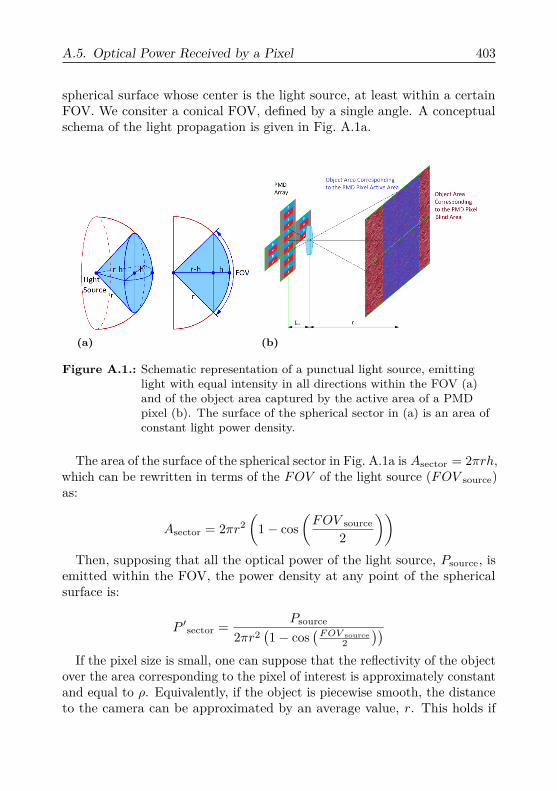
spherical surface whose center is the light source, at least within a certainFOV. We consiter a conical FOV, defined by a single angle. A conceptualschema of the light propagation is given in Fig. A.1a.

(a) (b)

Figure A.1.: Schematic representation of a punctual light source, emittinglight with equal intensity in all directions within the FOV (a)and of the object area captured by the active area of a PMDpixel (b). The surface of the spherical sector in (a) is an area ofconstant light power density.

The area of the surface of the spherical sector in Fig. A.1a is Asector = 2πrh,which can be rewritten in terms of the FOV of the light source (FOV source)as:

Asector = 2πr2(

1− cos(FOV source

2

))Then, supposing that all the optical power of the light source, Psource, is

emitted within the FOV, the power density at any point of the sphericalsurface is:

P ′sector = Psource

2πr2(1− cos

(FOV source

2))

If the pixel size is small, one can suppose that the reflectivity of the objectover the area corresponding to the pixel of interest is approximately constantand equal to ρ. Equivalently, if the object is piecewise smooth, the distanceto the camera can be approximated by an average value, r. This holds if

404 A. Appendix

the ratio between the r and flens (focal length of the lens) is not too large.Otherwise the pixel area would correspond to a large area in the object plane.From Fig. A.1b it is clear that, if the active area of the PMD pixel is of size[a× b]pixel, then the corresponding area in the object plane is [a× b]object,where: [

ab

]object

= r

flens

[ab

]pixel

Consequently, the object area reflecting the illumination light that iscaptured by the pixel can be derived from the pixel active area, Apixel, as:

Aobject =(

r

flens

)2Apixel

For a simplified schema of the active area of PMD pixels, we refer toFig. 2.8b. For a full characterization of the pixel response for the differentpixel areas, the reader is referred to Section 4.3.1. Clearly, the power reflectedby the the object region of area Aobject is:

Pobject = (P ′sectorAobject)ρ

If we suppose that the object is a Lambertian reflector, the light is notreflected with equal intensity in all directions, but it follows the so-calledLambert’s cosine law or Lambert’s emission law. According to it, the intensityalong a certain direction is directly proportional to the cosine of the anglebetween that direction and the surface normal. This is independent fromthe angle of incidence of the illumination. For simplicity, we suppose thatthe lens and the illumination are approximately in the same point, so thatwe can use r to denote also the distance from the object to the lens. In orderto obtain the power collected by the lens from that reflected by the object,the reflected light has to be integrated over the field collected by the lens.Supposing coaxiality between surface normal and principal axis of the lens,it can be showed that the optical power reaching the lens is given by:

Plens =(rlens

r

)2Pobject

where rlens is the radius of the lens aperture. We omit the demonstrationhere, since it has already been provided in [278]. If the power losses of theoptical system are modeled with an attenuation factor klens, then the powereffectively received at the sensitive area of the pixel is Ppixel = klensPlens,which, making use of the previous equalities, yields:

A.6. Experimental Evaluation of the Delay in the Illumination 405

Ppixel = Apixelρr2lensklens

2πr2f2lens(1− cos

(FOV source

2))Psource

= Apixelρklens

8π(rf#)2(1− cos

(FOV source

2))Psource

where f# = flens2rlens

is the f -number of the lens.

A.6. Experimental Evaluation of the DelayIntroduced in the Illumination ControlSignal in a ToF Camera with ModularIllumination

In this section we provide a brief summary of the experiments that werecarried out to find out the time delay that the Illumination Control Signal(ICS) experiences due to the cables and the electronics between the cameraand the LED and the LED itself. This is similar to the phase homogeneitytest performed in [278] for a simpler illumination system. The systemwe analyze is the medium-range ToF system of [283], which can provide amaximum optical power of 91 W in the NIR. The camera is a ZESS Multicam[216, 304], which integrates both a PMD and a color sensor in a single systemwith a common optical path. We focus on the illumination system, which iscomposed by 13 LED modules, with different orientations in an attempt toprovide a homogeneous illumination over a relatively wide FOV. Each LEDmodule features two LEDs, together with two independent control circuits,which are mostly signal amplifiers with a MOSFET for driving the LED.The LEDs are Osram SFH-4750, with 3.5 W optical power and an emissionspectrum between 775 nm and 900 nm, approximately, showing a narrowpeak at 856 nm. The LEDs are equipped with an optical grade PMMAcollimator of ±5.5 FWHM (Full Width at Half Maximum) half angle and38 mm diameter.

Several experiments were carried out, but here we refer only to one ofthem, in which the time delay between the ICS, generated by the MultiCam,and the optical signal emitted by each LED was calculated.

406 A. Appendix

A.6.1. MethodologyThe ICS is sensed at the entry of each LED module by means of electronicprobes, while the optical signal requires the use of a fast photodiode. Bothsignals are acquired simultaneously using an oscilloscope. The acquiredinterval is in the middle of one of the four pulse trains that are generatedper PMD acquisition. This way, the amplitude of the signals is stable duringthe acquisition. The results were found to be independent from in which ofthe four pulse trains the measurements are gathered. Consequently, we onlyprovide the results for one of them. Since both electrical input and opticaloutput are periodic signals of 20 MHz fundamental frequency, we cannotresolve delays greater than one period, i. e., 50 ns without ambiguity.

We use the center of gravity of the acquired waveforms as reference pointto calculate their relative shift. The position of a signal in time is given bythe abscissa of the center of gravity of the area under the curve, consideringonly one signal period. This way, we take into account not only delays dueto signal propagation, but also the effective delay, also due to slow risingand falling times of the LEDs and other signal distortions. The abscissa ofthe center of gravity can be calculated as

t =

∫ t0+T

t0

t s(t) dt∫ t0+T

t0

s(t) dt(A.8)

where s(t) is the periodic signal of period T , and t0 is a starting point, whichhas to be defined in the same way in both signals, e. g., detecting the start ofthe rising edge. This calculation is done for several signal periods, in orderto obtain mean values and standard deviations of the delays.

A.6.2. Experimental SetupA high-speed silicon fixed-gain photodetector (Thorlabs PDA10A-EC) with150 MHz bandwidth is used to sense the illumination signal. To this end, itis mounted on a tube (201 mm length, 30 mm diameter), equipped with aplain metallic adapter at the other side, that allows stable fixation to theLED modules. The tube avoids disturbance from neighboring LEDs andbackground light during the measurements. The spectral sensitivity of thephotodetector (200 nm and 1100 nm) ensures that all power emitted by theLED is being sensed. The output of the photo detector and of the ICS probes

A.6. Experimental Evaluation of the Delay in the Illumination 407

are connected using coaxial cables (of 1.5 m and 2 m length, respectively) toan oscilloscope (Tektronix TDS 3032B) of 300 MHz bandwidth and 2.5 Gs/sacquisition rate.One can argue that it would be easier to activate only the LED being

measured at a time, instead of using a tube to avoid interference betweenoptical signals, but this approach would modify the system with respect tothe normal operating conditions. Different load in the power line, togetherwith absence of eventual interferences between signals that might appear innormal operation, may lead to different delays. The complete ToF system ismounted on a rotary table, which is, in turn, fixed to a table. This allowsrotating the system with small angular steps and positioning the modules ina convenient position for measurement. The experimental setup is shown inFig. A.2.

Figure A.2.: Experimental setup for measuring the delay of the optical sig-nals with respect to the Illumination Control Signal (ICS). Theimages show the MultiCam, surrounded by the 13 double LEDmodules, mounted on a rotary table, fixed to the table. The tubu-lar coupling between LED module and photodetector ensuressensing only the desired signal, with minimal power loss. Theoscilloscope shows both the ICS and the photodetector output.

The two signals are acquired during 2µs at 2.5 gigasamples per second,i. e., around 40 periods per signal are considered. The same acquisitionprocedure is repeated for all 26 LEDs.

A.6.3. ResultsIn order to facilitate the presentation of results, the modules are numberedfrom 1 to 13 and the LEDs of each module are called upper or lower dependingon their position in the module. For clarity, a schema with the module

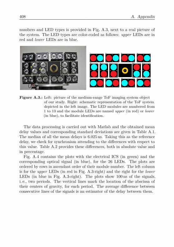
408 A. Appendix

numbers and LED types is provided in Fig. A.3, next to a real picture ofthe system. The LED types are color-coded as follows: upper LEDs are inred and lower LEDs are in blue.

Figure A.3.: Left: picture of the medium-range ToF imaging system objectof our study. Right: schematic representation of the ToF systemdepicted in the left image. The LED modules are numbered from1 to 13 and the module LEDs are named upper (in red) or lower(in blue), to facilitate identification.

The data processing is carried out with Matlab and the obtained meandelay values and corresponding standard deviations are given in Table A.1.The median of all the mean delays is 6.025 ns. Taking this as the referencedelay, we check for synchronism attending to the differences with respect tothis value. Table A.2 provides these differences, both in absolute value andin percentage.Fig. A.4 contains the plots with the electrical ICS (in green) and the

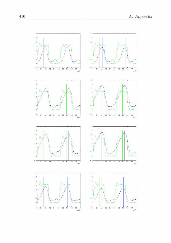
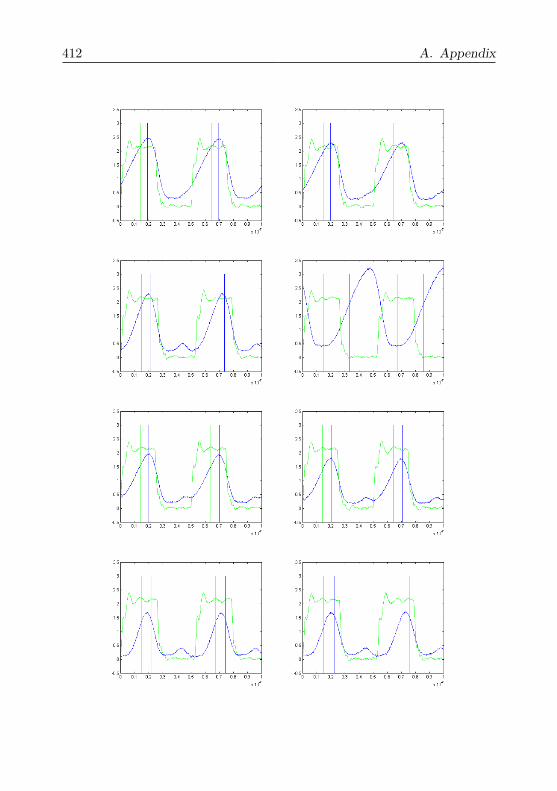
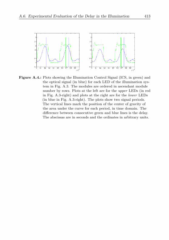
corresponding optical signal (in blue), for the 26 LEDs. The plots areordered by rows in ascendant order of their module number. The left columnis for the upper LEDs (in red in Fig. A.3-right) and the right for the lowerLEDs (in blue in Fig. A.3-right). The plots show 100 ns of the signals,i. e., two periods. The vertical lines mark the location of the abscissa oftheir centers of gravity, for each period. The average difference betweenconsecutive lines of the signals is an estimator of the delay between them.

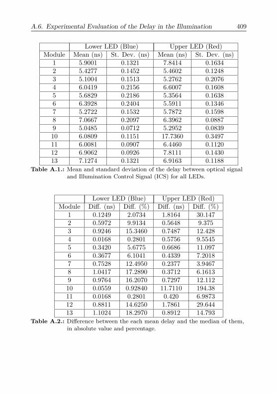
A.6. Experimental Evaluation of the Delay in the Illumination 409

Lower LED (Blue) Upper LED (Red)Module Mean (ns) St. Dev. (ns) Mean (ns) St. Dev. (ns)

1 5.9001 0.1321 7.8414 0.16342 5.4277 0.1452 5.4602 0.12483 5.1004 0.1513 5.2762 0.20764 6.0419 0.2156 6.6007 0.16085 5.6829 0.2186 5.3564 0.16386 6.3928 0.2404 5.5911 0.13467 5.2722 0.1532 5.7872 0.15988 7.0667 0.2097 6.3962 0.08879 5.0485 0.0712 5.2952 0.083910 6.0809 0.1151 17.7360 0.349711 6.0081 0.0907 6.4460 0.112012 6.9062 0.0926 7.8111 0.143013 7.1274 0.1321 6.9163 0.1188

Table A.1.: Mean and standard deviation of the delay between optical signaland Illumination Control Signal (ICS) for all LEDs.

Lower LED (Blue) Upper LED (Red)Module Diff. (ns) Diff. (%) Diff. (ns) Diff. (%)

1 0.1249 2.0734 1.8164 30.1472 0.5972 9.9134 0.5648 9.3753 0.9246 15.3460 0.7487 12.4284 0.0168 0.2801 0.5756 9.55455 0.3420 5.6775 0.6686 11.0976 0.3677 6.1041 0.4339 7.20187 0.7528 12.4950 0.2377 3.94678 1.0417 17.2890 0.3712 6.16139 0.9764 16.2070 0.7297 12.11210 0.0559 0.92840 11.7110 194.3811 0.0168 0.2801 0.420 6.987312 0.8811 14.6250 1.7861 29.64413 1.1024 18.2970 0.8912 14.793

Table A.2.: Difference between the each mean delay and the median of them,in absolute value and percentage.

410 A. Appendix

A.6. Experimental Evaluation of the Delay in the Illumination 411

412 A. Appendix

A.6. Experimental Evaluation of the Delay in the Illumination 413

Figure A.4.: Plots showing the Illumination Control Signal (ICS, in green) andthe optical signal (in blue) for each LED of the illumination sys-tem in Fig. A.3. The modules are ordered in ascendant modulenumber by rows. Plots at the left are for the upper LEDs (in redin Fig. A.3-right) and plots at the right are for the lower LEDs(in blue in Fig. A.3-right). The plots show two signal periods.The vertical lines mark the position of the center of gravity ofthe area under the curve for each period, in time domain. Thedifference between consecutive green and blue lines is the delay.The abscissas are in seconds and the ordinates in arbitrary units.

414 A. Appendix

A.7. Mutual and Matrix CoherencesThis section provides the proofs of Eq. 3.40 and Eq. 3.52. Eq. 3.40 providesa lower bound on the mutual coherence between rows of the sensing matrixΦΦΦ and columns of the dictionary ΨΨΨ in the very specific case of ΨΨΨ ∈ Rn×nbeing an orthonormal basis of Rn by columns and the rows of ΦΦΦ ∈ Rm×nbeing selected from another orthonormal basis of Rn. Provided that ΨΨΨ is anorthonormal basis of the space, any n-dimensional vector can be expressedin terms of the basis elements without power loss. Specifically, for the rowsof ΦΦΦ we can write

n∑j=1

∣∣∣〈~φi, ~ψj〉∣∣∣2 = 1, ∀1 ≤ i ≤ m

where ~φi denotes the ith row of ΦΦΦ and ~ψj denotes the jth column of ΨΨΨ. Theinner product in this expression provides the bridge towards the mutualcoherence (recall Eq. 3.39) and a lower bound on the sum can be triviallyestablished by substituting each term by that of maximum value, that is:

n∑j=1

∣∣∣〈~φi, ~ψj〉∣∣∣2 = 1 ≤n∑j=1

maxj

∣∣∣〈~φi, ~ψj〉∣∣∣2 = nmaxj

∣∣∣〈~φi, ~ψj〉∣∣∣2 , ∀1 ≤ i ≤ mProvided that the previous inequality holds ∀i, the maximization can be

extended also along i and the inequality remains true, yielding

1 ≤ nmaxi,j

∣∣∣〈~φi, ~ψj〉∣∣∣2 , ∀1 ≤ i ≤ m, 1 ≤ j ≤ n

and from Eq. 3.39 immediately follows

1√n≤ µ (ΦΦΦ,ΨΨΨ) ≤ 1

Let’s now derive the general lower bound on µ (AAA) given in Eq. 3.52 forthe case of ΦΦΦ with unit norm rows and ΨΨΨ with unit norm columns, withoutany further hypothesis on the resulting measurement matrix AAA = ΦΦΦΨΨΨ. Thenormalization requirement is just for simplification of the derivations, sinceit allows omitting the denominator in the right hand side of Eq. 3.39. Let’sstart rewriting the dot product between two different columns of AAA in termsof ΦΦΦ and ΨΨΨ:

A.7. Mutual and Matrix Coherences 415

|〈~ai,~aj〉| =∣∣∣(~ψ>i ΦΦΦ>

)(ΦΦΦ~ψj

)∣∣∣=

∣∣∣∣∣∣∣∣∣[〈~ψ>i , ~φ>1 〉 〈~ψ>i , ~φ>2 〉 . . . 〈~ψ>i , ~φ>m〉

]〈~φ1, ~ψj〉〈~φ2, ~ψj〉

...〈~φm, ~ψj〉

∣∣∣∣∣∣∣∣∣

=

∣∣∣∣∣m∑k=1〈~φk, ~ψi〉〈~φk, ~ψj〉

∣∣∣∣∣By means of a recursive triangular inequality, the absolute value of the

summation in last line of the previous expression can be used as a lowerbound for the corresponding sum of absolute values, namely,

|〈~ai,~aj〉| =

∣∣∣∣∣m∑k=1〈~φk, ~ψi〉〈~φk, ~ψj〉

∣∣∣∣∣ ≤m∑k=1

∣∣∣〈~φk, ~ψi〉∣∣∣ ∣∣∣〈~φk, ~ψj〉∣∣∣Clearly, each term in the latter sum is upper-bounded by the mutual

coherence, as defined in Eq. 3.39. Therefore, we have that

|〈~ai,~aj〉| ≤m∑k=1

∣∣∣〈~φk, ~ψi〉∣∣∣ ∣∣∣〈~φk, ~ψj〉∣∣∣ ≤ mµ2 (ΦΦΦ,ΨΨΨ)

Dividing both sides of the latter inequality by ‖~ai‖2‖~aj‖2 6= 0 and seekingthe maximum value among all possible column pairs with i 6= j yields

maxi<j

|〈~ai, ~aj〉|‖~ai‖2‖~aj‖2

≤ maxi<j

mµ2 (ΦΦΦ,ΨΨΨ)‖~ai‖2‖~aj‖2

Clearly, the left hand term is the matrix coherence of AAA, µ (AAA), as definedin Eq. 3.42. Additionally, suppose that there exists a nonzero lower boundC on the l2 norm of the columns of AAA, which has to be true, unless somecolumn of AAA is the zero vector. Note that the latter case is inadmissible inpractice, since it would imply that the sparse coefficient corresponding tothe dictionary atom for which the corresponding column of AAA is null cannotbe retrieved. Then, one can immediately obtain Eq. 3.52 from the previousinequality:

416 A. Appendix

µ (AAA) ≤ 1C2mµ

2 (ΦΦΦ,ΨΨΨ)

C = min1≤i≤n

‖~ai‖2

A.8. Adaptive High Dynamic Range:Complementary Material

This section complements the experimental evaluation of the Adaptive HDRmethod presented in Section 4.2.2.4 with some additional material that wasomitted in that section for brevity.

A.8.1. Böhler Star DetailThe inclusion of Böhler stars in Exp. 1 of Section 4.2.2.4 has as objectivecomparing the different experimental cases in terms of lateral resolution. Asstated in that section, our AHDR approach brings an improvement of theeffective lateral resolution (see Table 4.1) of ToF cameras. Such improvementbecomes perceptible in, e. g., the lower Böhler star of the panel in the imagesof Fig. 4.10. For the sake of clarity, in Fig. A.5 we provide a detail ofthe depth images of the star, for the two single exposures and our AHDRapproach, together with a reference color image of the Böhler star. The caseof exhaustive HDR has been omitted, but the corresponding result does notdiffer much from Fig. A.5c. Our adaptive approach (Fig. A.5d) performsvisibly better than a single acquisition with an exposure time adapted tothe stars panel (0.1 ms, Fig. A.5c).

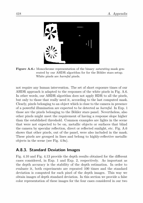
A.8.2. Saturating MaskThe so-called saturating mask is just a 2D representation of the set ofall pixels considered harmful. As explained in Section 4.2.2.3, a pixel isconsidered harmful if the slope of the response curve in exposure domain ishigher than a threshold, for any of the channels, at any of the four doubleraw images. There is only one mask per set of PMD raw images. Theharmful pixels are stored as ones in the mask and the rest as zeros. In orderto provide a better understanding of the mask, Fig. A.6 depicts the maskobtained in Exp. 1. The corresponding scene is depicted in Fig. 4.9a.

Despite its sharpness, recall that the mask is automatically generated froma considerable amount of raw data taken at different exposures and does

A.8. Adaptive High Dynamic Range: Complementary Material 417

(a) Color Image (b) Single Exposure: 2 ms

(c) Single Exposure: 0.1 ms (d) AHDR

Figure A.5.: Detail of the depth estimation for the lower Böhler star of thepanel in Exp. 1. The images are a detail of the corresponding im-ages in Fig. 4.10. The results obtained from two single-exposureacquisitions at 2 ms (b) and 0.1 ms (c) are compared to the resultof our AHDR approach (d). The result of the intensive HDR al-gorithm is omitted to include a frontal color image of the star (a).It is hard to recognize any 3D structure in (b) without the helpof (a). c©2015 IEEE.

418 A. Appendix

Figure A.6.: Monochrome representation of the binary saturating mask gen-erated by our AHDR algorithm for for the Böhler stars setup.White pixels are harmful pixels.

not require any human intervention. The set of short exposure times of ourAHDR approach is adapted to the responses of the white pixels in Fig. A.6.In other words, our AHDR algorithm does not apply HDR to all the pixels,but only to those that really need it, according to the last computed mask.Clearly, pixels belonging to an object which is close to the camera in presenceof a powerful illumination are expected to be detected as harmful. In Exp. 1those are the pixels belonging to the Böhler stars panel. Nevertheless, alsoother pixels might meet the requirement of having a response slope higherthan the established threshold. Common examples are lights in the scenethat were not expected to be on, metallic objects or surfaces that blindthe camera by specular reflection, direct or reflected sunlight, etc. Fig. A.6shows that other pixels, out of the panel, were also included in the mask.These pixels are grouped in lines and belong to highly-reflective metallicobjects in the scene (see Fig. 4.9a).

A.8.3. Standard Deviation ImagesFig. 4.10 and Fig. 4.13 provide the depth results obtained for the differentcases considered, in Exp. 1 and Exp. 2, respectively. As important asthe depth accuracy is the stability of the depth estimation. In order toevaluate it, both experiments are repeated 100 times and the standarddeviation is computed for each pixel of the depth images. This way weobtain images of depth standard deviation. In this section we provide a falsecolor representation of these images for the four cases considered in our two

A.8. Adaptive High Dynamic Range: Complementary Material 419

experimental setups, namely, the exhaustive HDR algorithm, two cases ofsingle acquisition at short and long exposure times and our Adaptive HighDynamic Range (AHDR) approach.

A.8.3.1. Böhler Stars Experiment

In this section standard deviation images for each of the depth imagescomputed in the Exp. 1 of Section 4.2.2.4 (corridor with Böhler stars) areprovided. The results are represented as false color images in Fig. A.7. Thisfigure complements Fig. 4.10 by providing per-pixel depth uncertainty.Fig. A.7a is the standard deviation image delivered by the exhaustive

HDR algorithm presented in Section 4.2.2.1 using a dataset of 200 raw imagesets, acquired at exposure times from 0.01 to 2 ms, with 0.01 ms step. Thisimage should be taken as a reference of lowest deviation, so that the closerwe get to this result, the better our method is. Note the extremely lowdeviations: below 5mm for most pixels and submillimetric for some pixelsbelonging to the Böhler stars panel. The false color range is [0, 0.01] m.Fig. A.7b shows the result obtained for a fixed exposure time of 2 ms,

which is proper for sensing the corridor but not the panel with the Böhlerstars. Indeed, subcentimetric deviations are observed for many pixels of thefrontal wall, even when some pixels exhibit depth measurements higher than14 m. In contrast, some pixels of the Böhler stars panel exhibit deviationshigher than 1 cm, due to SBI-related noise. Note that the noise patternobserved in Fig. 4.10b coincides with that present in Fig. A.7b, i. e., pixelswith high depth error due to SBI limited operative range also show lowstability. In general, for this exposure time, the overall result is good fora PMD-based camera in terms of standard deviation, below 4 cm for mostpixels.

The complementary case to the previous uses an exposure time adapted tothe Böhler stars panel, at one meter from the camera. As one could expectand can be observed in Fig. A.7c, this leads to very low standard deviationsfor the panel surface (mostly below 1 cm), at the cost of huge deviationsalong the rest of the scene (typically over 20 cm), also in coherence withFig. 4.10c. Note that the range of the false color representation has beenchanged to [0, 0.5] m, in order to avoid an appearance of binary image.Finally, the standard deviation image obtained for our AHDR algorithm

is shown in Fig. A.7d. The short exposure times used to accurately sensethe Böhler stars panel allow subcentimetric deviations in the panel surface,sometimes lower than 2 mm. The rest of the scene offers a deviation dis-tribution coincident with that shown in Fig. A.7b, since only raw images

420 A. Appendix

(a) HDR (b) Single Exposure: 2 ms

(c) Single Exposure: 0.1 ms (d) AHDR

Figure A.7.: Standard deviation images obtained from 100 different executionsof Exp. 1. The corresponding MultiCam color image is given inFig. 4.9a. The reference standard deviation image, obtained fromthe result of the intensive HDR algorithm is shown in (a). Twocases of single exposure times of 2 ms and 0.1 ms are given in (b)and (c), respectively. In both cases no HDR algorithm is applied.Finally, (d) shows the depth standard deviation image obtainedwhen applying our AHDR approach. c©2015 IEEE.

A.8. Adaptive High Dynamic Range: Complementary Material 421

acquired at the reference exposure time (2 ms, in this case) are used for thepixels not contained in the saturating mask. In both figures the false colorrange is [0, 0.1] m.

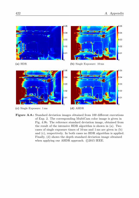
A.8.3.2. Laboratory Experiment

The standard deviation results we present in this section correspond to theExp. 2 of Section 4.2.2.4. The results are depicted in four false color imagesin Fig. A.8.Fig. A.8a is to be taken as reference and shows the standard deviation

image obtained when applying the basic HDR algorithm to a dataset of 100raw image sets, acquired at exposure times from 0.1 to 10 ms, with 0.1 msstep. Fig. A.8b is the result obtained for a fixed exposure time of 10 ms,which is appropriate for sensing the large scene. The standard deviationresult is coherent with Fig. 4.13b. Relatively low standard deviations areobserved for the far background (typically lower than 1 cm). Note the higherdeviations registered for pixels lying on planes that are not perpendicularto the illumination direction, such as ceiling or lateral walls. Also from thestandard deviation image it is clear that there is a problem with the depthestimation for the apple pixels for such a high exposure time. Very diversestandard deviations are registered in this area, breaking the smoothness ofthe deviation image. Values go from 0.28 mm up to 1.23 cm.

The standard deviations registered for the complementary case, i. e., depthestimation using a single acquisition at short exposure time, are depicted inFig. A.8c. As one could expect, the deviation is lower for those areas thatare close to the camera, e.g., the apple or the table. Note that the irregulardeviation values registered for the apple in Fig. 4.13b are not present inFig. A.8c, due to the absence of saturation. Values vary from as little as0.1 mm up to 2 mm, suggesting an accurate depth estimation.Finally, Fig. A.8d confirms the good quality of the results delivered by

our AHDR algorithm. Note the smooth distribution over the apple surface,very close to the result obtained for exhaustive HDR (Fig. A.8a), which istaken as reference. All apple pixels but one show a standard deviation lowerthan 5 mm.

A.8.4. Runtime ResultsAs explained in the Section 4.2.2.3, when the scene change due to theintroduction of an intrusive object close to the camera is detected, theadaptation process is triggered. A dense dataset of raw image sets at

422 A. Appendix

(a) HDR (b) Single Exposure: 10 ms

(c) Single Exposure: 1 ms (d) AHDR

Figure A.8.: Standard deviation images obtained from 100 different executionsof Exp. 2. The corresponding MultiCam color image is given inFig. 4.9b. The reference standard deviation image, obtained fromthe result of the intensive HDR algorithm is shown in (a). Twocases of single exposure times of 10 ms and 1 ms are given in (b)and (c), respectively. In both cases no HDR algorithm is applied.Finally, (d) shows the depth standard deviation image obtainedwhen applying our AHDR approach. c©2015 IEEE.

A.9. Inverse Freeman-Tukey Transformation for Poisson Data 423

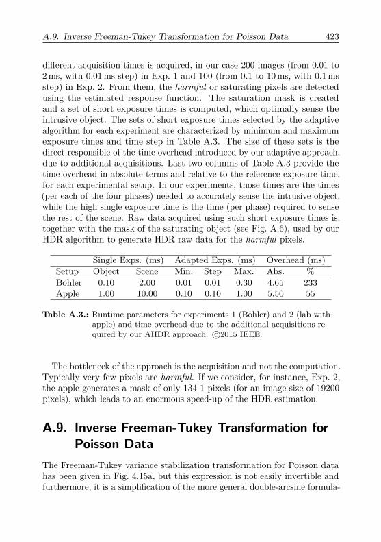
different acquisition times is acquired, in our case 200 images (from 0.01 to2 ms, with 0.01 ms step) in Exp. 1 and 100 (from 0.1 to 10 ms, with 0.1 msstep) in Exp. 2. From them, the harmful or saturating pixels are detectedusing the estimated response function. The saturation mask is createdand a set of short exposure times is computed, which optimally sense theintrusive object. The sets of short exposure times selected by the adaptivealgorithm for each experiment are characterized by minimum and maximumexposure times and time step in Table A.3. The size of these sets is thedirect responsible of the time overhead introduced by our adaptive approach,due to additional acquisitions. Last two columns of Table A.3 provide thetime overhead in absolute terms and relative to the reference exposure time,for each experimental setup. In our experiments, those times are the times(per each of the four phases) needed to accurately sense the intrusive object,while the high single exposure time is the time (per phase) required to sensethe rest of the scene. Raw data acquired using such short exposure times is,together with the mask of the saturating object (see Fig. A.6), used by ourHDR algorithm to generate HDR raw data for the harmful pixels.

Single Exps. (ms) Adapted Exps. (ms) Overhead (ms)Setup Object Scene Min. Step Max. Abs. %Böhler 0.10 2.00 0.01 0.01 0.30 4.65 233Apple 1.00 10.00 0.10 0.10 1.00 5.50 55

Table A.3.: Runtime parameters for experiments 1 (Böhler) and 2 (lab withapple) and time overhead due to the additional acquisitions re-quired by our AHDR approach. c©2015 IEEE.

The bottleneck of the approach is the acquisition and not the computation.Typically very few pixels are harmful. If we consider, for instance, Exp. 2,the apple generates a mask of only 134 1-pixels (for an image size of 19200pixels), which leads to an enormous speed-up of the HDR estimation.

A.9. Inverse Freeman-Tukey Transformation forPoisson Data

The Freeman-Tukey variance stabilization transformation for Poisson datahas been given in Fig. 4.15a, but this expression is not easily invertible andfurthermore, it is a simplification of the more general double-arcsine formula-

424 A. Appendix

tion, for binomial distributions. Profiting from trigonometric identities, it hasbeen shown that the Freeman-Tukey double-arcsine transformation (Eq. A.9)admits a closed-form inverse transformation [328], given by Eq. A.10,

t = arcsin√

λ

n+ 1 + arcsin√λ+ 1n+ 1 (A.9)

p(t) = 12

1− sgn (cos t)

√1−

[sin t+ 1

n

(sin t− 1

sin t

)]2 (A.10)

where p and n are the parameters of the binomial distribution B(n, p), namely,probability of success and number of independent experiments. Recall thatthe Poisson distribution is a limit case of the binomial distribution, whenp → 0 and n → ∞. In the Poisson case, P (λ), we are interested inthe number of occurrences or successes, λ = p n. The direct Freeman-Tukey transformation for the Poisson case can be derived from Eq. A.9 asy = lim

n→∞

√n+ 1 t. Consequently, we can pursuit an inverse transformation

x(y) for the Poisson case from Eq. A.10 as:

x(y) = lim(t= y√

n+1

)n→∞

n p(t)

We substitute p(t) in the previous expression by Eq. A.10 and make use of

the trigonometric limit approximation limε→0

sin ε ' ε− ε3

6 , which derives fromthe corresponding Taylor expansion, neglecting the terms of order equal orhigher than five. We obtain the following polynomial:

x(y) = lim(t= y√

n+1

)n→∞

n

2

1−

√1−

(n t+ 5t

6 −1t

n

)2

Note that the signature of the cosine has been left away, since in thePoisson case: lim

ε→0cos ε = 1. At this point, we get rid of the square root by

using the limit approximation limε→0

√1− ε ' ε− ε

2 , which derives, in turn,from the first order Taylor expansion. Substituting and operating we get:

x(y) = lim(t= y√

n+1

)n→∞

14

(√n t+ 5t

6√n− 1t√n

)2

A.10. Fluorescence Lifetime Microscopy and ToF Imaging 425

Executing the implicit changes of variables t = y√n+1 , we get a function

of the transformed variable, y:

x(y) = limn→∞

14

( √n√

n+ 1y + 5

6√n√n+ 1

y −√n+ 1√n

y−1)2

The limit can be now trivially calculated, yielding the inverse transforma-tion presented in Eq. 4.16:

x(y) =(y − y−1

2

)2

A.10. Fluorescence Lifetime Microscopy and ToFImaging

Fluorescence is the phenomenon of light emission by an atom or moleculeshortly after the absorption of photons, typically < 10−8 s [276]. This effectcan be exploited, for instance, to enhance the contrast in biological andmedical imaging, by using fluorophores. The emitted radiation is always oflower energy than the excitation radiation, that is, there is a shift towardshigher wavelengths, known as Stokes’ shift in honor to George Gabriel Stokes,who introduced the term fluorescence in the mid 19th century.

The intrinsic properties of a fluorophore include [322] quantum efficiency,fluorescence decay profile in time domain, the excitation and emission spectraand the response to polarized light. From these properties, the decay profileis of great importance, since determining it allows recognizing the materialproducing the fluorescence or, at least, making it distinguishable fromneighboring or background materials. Suppose that the fluorescent materialis excited with a pulse of light that describes a Dirac delta function in timedomain. The resulting time-dependent emission is the impulse responsefunction, which can be accurately described as a sum of exponential functions.A common way of parameterizing this function is given by:

iδ(t) =∑i

αie− tτi (A.11)

where αi are the preexponential factors and τi the decay times. Eq. A.11 isable to represent almost any decay law, but if the decay is purely exponential,a single exponential function suffices and only a pair of parameters, α, τ isto be determined. In logarithmic scale, it is easy to observe that log iδ(t) is

426 A. Appendix

a linear function of time, with offset α and slope − 1τ . If the material is a

mix of few fluorophores with a single decay time, each τi in Eq. A.11 is thedecay time of each component. Obviously, if the constituent decay times aretoo closely spaced, resolving them becomes challenging.From now on we focus on the case of a single decay time. In order to

obtain the parameters characterizing the decay profile, measurements aregathered either in time-domain or in frequency-domain. In time-domainfluorometry, the sample is excited with a short pulse of light, as close aspossible to a Dirac delta function, and the time-dependent intensity of theemitted light is recorded. From these intensity measurements the offsetand slope of log iδ(t) can be calculated, yielding the parameters α, τ . If thedecay times are of few nanoseconds, data acquisition at a very high samplingrate becomes necessary to obtain an acceptable number of sample points ofiδ(t). To circumvent that difficulty, MCP PMTs or fast SPADs are used incombination with modern TCSPC boards, which can already offer jitters of< 1 ps [35]. The basic principle of TCSPC is to emit the excitation pulserepeatedly and register the arrival of photons emitted by the sample andtheir time of arrival with respect to the time of emission of the excitationpulse. This way, very accurate decay profiles can be obtained, as a histogramof photon time of arrival generated by pulse repetition.

Alternatively, fluorometry can be carried out in frequency domain, in whichcase the sample is excited with intensity-modulated light, typically accordingto a sinusoidal waveform. The emitted waveform is the convolution of theexcitation one with the decay function, which is an exponential or a sum ofexponential functions. Regardless of the shape of the decay function, if theexcitation is sinusoidally-modulated, the resulting waveform is also sinusoidal,with rescaled amplitude and phase-shifted. For a single-exponential decay,the decay time τ can be calculated using a single modulation frequency fmodas

τ = tan ∆φ2πfmod

(A.12)

where ∆φ denotes phase shift. A derivation of Eq. A.12 can be found in[276]. This method is also known as phase modulation.

Parallelism With ToF Depth Imaging As in fluorometry, ToF systemsmay also operate in time or frequency domains. For instance, pulsed systemswith SPADs for detecting the echo arrival operate natively in time domain,while PMD pixels require continuous emission of sinusoidally-modulated

A.10. Fluorescence Lifetime Microscopy and ToF Imaging 427

light to compute the phase shift that the depth to measure causes in theecho. In phase-shift-based ToF systems, the response function of the scenecan be modeled as a Dirac delta function (Eq. 2.8) or as a sum of Dirac deltafunctions in presence of MPI (see the multipath paragraph in Section 2.4.1for details on MPI).

Note the similarity between the environment response function for a ToFsystem in the case of a finite number of paths (Eq. 4.32) and Eq. A.11.Actually, if the scene response is modeled as a weighted sum of exponen-tial functions, both responses coincide. This is not a meaningless idea,since diffuse MPI offen lead to close-to-exponential environmental responses.In [221], modeling the environmental response as a sum of exponentially-modified Gaussian functions allow facing both specular and diffuse MPI andenables ToF depth imaging in scattering media. The exponentially-modifiedGaussian is obtained via convolution of the Gaussian and exponential func-tions. Consequently, it models both an exponential decay and a Gaussianlow-pass filter, which can be related to the limited bandwidth of the mea-surement instruments. In other words, exponential decays may appear asexponentially-modified Gaussian functions when measured. Consequently,methods as that in [221] are transferable to fluorometry.

Conceptually, phase-modulation-based fluorometry and phase-shift-baseddepth sensing are equivalent, since in both cases the information we wantto retrieve is conveyed by the phase shift undergone by a AMCW lightsignal. Once the phase shift is computed, Eq. A.12 yields the decay timein fluorometry, while Eq. 2.1 yields the depth in depth sensing. NowadaysTCSPC boards offer one to four parallel channels, while using a, e. g., 19kPMD chip would be equivalent to have 19.2× 103 parallel channels.

Therefore, the question that arises is: can TCSPC systems be successfullysubstituted by commercial ToF cameras? The answer depends on theapplication. The use of PMD chips poses a limitation in the maximummodulation frequency. If the decay is too fast, the phase resolution offeredby a PMD device may be insufficient to resolve the phase shift. Accordingto [370], the optimal modulation frequency of the excitation signal to sensea fluorophore of decay time τ is 1

10τ . Consequently, if the decay times are inthe nanosecond range, using a PMD array as detector is feasible and allowsgenerating large FLIM images while achieving very short acquisition times.For instance, supposing an exposure time for the PMD chip of 1 ms andnegligible positioning times of the stepper unit, a FLIM image of 19 Mpixcould be obtained in one second. This is far beyond the acquisition rates ofsingle-channel TCSPC systems, which typically need few seconds to gatherimages of few thousand pixels. Conversely, one could obtain a stream of

428 A. Appendix

FLIM video with moderate resolution in real time.

Related Work Already in the early years of the PMD technology, FLIMwas presented as a potential application, patented in [187]. In [173] theSwissRanger SR-2 ToF sensor, with 124× 160 pixels (equivalent to a PMD19k), is used as detector in a FLIM setup. Eight equally-spaced phases, i. e.,π4 phase step, are acquired and the phase shift is computed as usually usingEq. 2.6.

A complete mathematical formulation for the use of a ToF sensor in FLIMis given in [44], where the excitation signal is only required to be periodic,which allows for unified expressions for both TD-FLIM (periodically repeateddelta functions) and FD-FLIM (sinusoidal modulation). They also model theemitted signal as a convolution between the excitation signal and a certainresponse function. In order to account for a depth displacement betweensample and sensor, the sample response function is a displaced exponential,where the displacement corresponds to the depth, as in conventional ToF.Additionally, since reflected excitation light that did not cause emission canalso reach the sensor, the total response function is modeled as the sum of adepth-related (delta) response function and the sample-related (exponential)response function. This last consideration can be discarded if an opticalfilter is used to block the excitation wavelength.

The main contribution of [44] is to provide general frameworks for recover-ing the decay time τ and an eventual depth displacement of the sample dmod.Both in TD-FLIM and FD-FLIM the problem is solved via minimization ofan error function that measures the distance between the observations andmodel predictions in an appropriate domain (response domain in TD-FLIMand phase domain in FD-FLIM). The FLIM-oriented camera introduced byPCOr [176] features a proprietary CMOS ToF chip with 1008×1008 pixels.The pixel principle of operation coincides with that of PMD pixels and thecamera performs FD-FLIM with 40 MHz maximum modulation frequency.

A.11. The CS-PMD Camera PrototypeThe goal of this section is to provide a visual overview of the CS-PMDcamera prototype, complementing the general hardware description givenin Section 5.2. The prototype is built on a rail, to ensure perfect align-ment between the optical elements and accurate mechanical adjustments.Fig. A.9 shows a front view of the system, where all principal componentsare visible. We refer to Fig. 5.4 for understanding of the setup. In short

A.11. The CS-PMD Camera Prototype 429

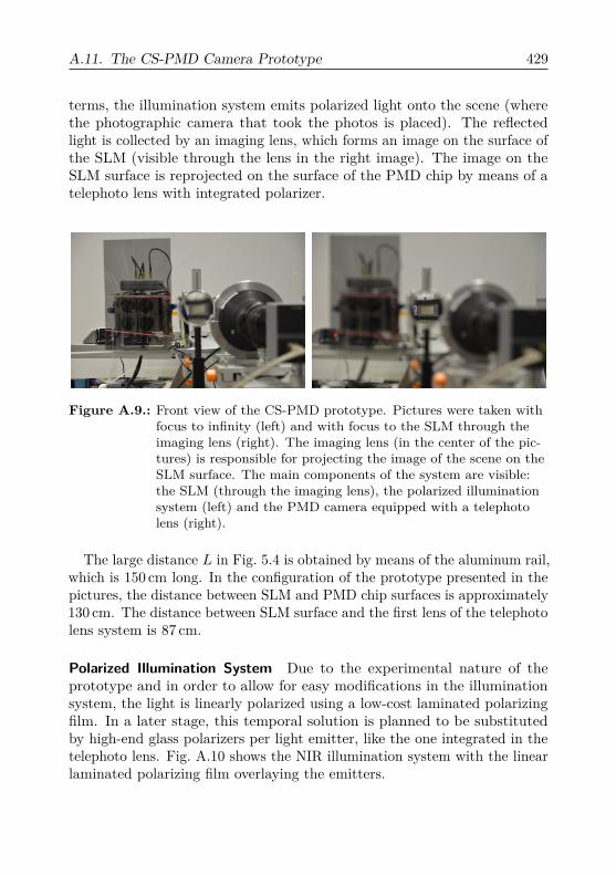
terms, the illumination system emits polarized light onto the scene (wherethe photographic camera that took the photos is placed). The reflectedlight is collected by an imaging lens, which forms an image on the surface ofthe SLM (visible through the lens in the right image). The image on theSLM surface is reprojected on the surface of the PMD chip by means of atelephoto lens with integrated polarizer.

Figure A.9.: Front view of the CS-PMD prototype. Pictures were taken withfocus to infinity (left) and with focus to the SLM through theimaging lens (right). The imaging lens (in the center of the pic-tures) is responsible for projecting the image of the scene on theSLM surface. The main components of the system are visible:the SLM (through the imaging lens), the polarized illuminationsystem (left) and the PMD camera equipped with a telephotolens (right).

The large distance L in Fig. 5.4 is obtained by means of the aluminum rail,which is 150 cm long. In the configuration of the prototype presented in thepictures, the distance between SLM and PMD chip surfaces is approximately130 cm. The distance between SLM surface and the first lens of the telephotolens system is 87 cm.

Polarized Illumination System Due to the experimental nature of theprototype and in order to allow for easy modifications in the illuminationsystem, the light is linearly polarized using a low-cost laminated polarizingfilm. In a later stage, this temporal solution is planned to be substitutedby high-end glass polarizers per light emitter, like the one integrated in thetelephoto lens. Fig. A.10 shows the NIR illumination system with the linearlaminated polarizing film overlaying the emitters.

430 A. Appendix

(a) (b)

Figure A.10.: Front view of the polarized illumination system (a) and detailof the emitters (b). The system is mounted on an arm that isfirmly attached to the main rail. The arm location can be ad-justed parallelly to the rail and the illumination system can bedisplaced linearly along the arm and rotated along the verticalaxis, normal to the plane defined by the rail and the arm. Eachemitter is equipped with a collimator to restrict the FOV of theillumination to that of the camera.

The illumination system in mounted on an arm, which is firmly attached tothe rail at a position that can be adjusted (Fig. A.10a). The location of thesystem on the arm and its yaw can also be adjusted, so that it appropriatelyilluminates the scene observed by the CS-PMD camera. The illuminationmodules are similar to those of the medium-range illumination system [283]analyzed in Appendix A.6. Our system features only two modules, orientedvertically. Each module has two NIR emitters with independent controlcircuits, still driven by the same ICS. The NIR emitters are also the OsramSFH-4750 LEDs, with 3.5 W optical power and a narrow emission peak at856 nm. Consequently, the maximum optical power of the system is 14 W. Inorder to adjust the FOV of the illumination system to that of the CS-PMDcamera, all LEDs are equipped with an optical grade PMMA collimator of±2 FWHM (Full Width at Half Maximum) half angle and 38 mm diameter.The optical efficiency of the collimator is 92%. Both illumination modules aresynchronously driven by the ICS signal coming from the CS-PMD moduleof the camera.

A.11. The CS-PMD Camera Prototype 431

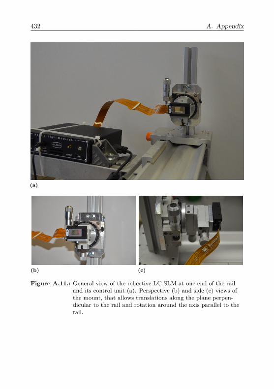
Spatial Modulation: LC-SLM As introduced in Section 5.2, the 2D spatialcodes are superimposed to the scene image by means of a reflective LC-SLM,before reprojection on the PMD chip. The SLM is a Holoeye LC-R 1080,featuring an array of 1200 × 1920 pixels with 90% fill factor. The SLMis reconfigured to a resolution of 1200 × 1600 (160 inactive SLM columnsat both sides of the array), in order to fit the aspect ratio of the PMDarray. The SLM is mounted at one end of the rail by means of a platformwith a special mount that allows accurately positioning and orienting theSLM. Ideally, the SLM and PMD surfaces should be parallel and the centersof their respective active areas aligned along the same normal. Fig. A.11provides images of the SLM and the adjustable mount.

The mount allows displacements along the vertical and horizontal axes ofthe SLM (perpendicular to the rail direction) with micrometer resolution.To this end, two translation stages with manual adjustment are mountedon top of each other along the desired directions (Fig. A.11c). Additionally,rotation of the SLM around the axis parallel to the rail (perpendicular tothe previous two) is achieved by means of a rotation stage with minuteresolution (Fig. A.11b). Both the translational stages and the rotational oneare adjusted by hand via their respective fine-adjustment screws.

PMD Camera with Telephoto Lens The image at the SLM is reprojectedon the PMD ship by means of a telephoto lens. We use a Nikon Nikkor ED300mm 1:2.8 objective. The lens system includes 11 elements in 9 groups plusa dust-proof glass plate before the first element. The diameter of the firstlens is approximately 110 mm. The objective has a built-in port for drop-inpolarizers and filters (see Fig. A.12b), where we place a linear polarizer. Inorder to maximize the contrast, the orientation of the polarizer has to becarefully adjusted so that it is either the same or crossed with respect tothat of the polarizer of the illumination system. The Nikon F mount ofthe objective is adapted to the C-mount of the MultiCam housing we usefor our CS-PMD camera by means of a Hama adapter. Additionally, inorder to restrict the FOV to the small SLM window, we make use of threeC-mount extension tubes of 40 mm each, located between the adapter andthe camera. Thanks to the extension, one can meet the requirement of alarge L (Fig. 5.4) and a restricted FOV. Fig. A.12a shows the CS-PMDcamera with the objective.

The linear polarizer that is integrated in the telephoto lens system is thehight transmittance Heliopan Polfilter 8015 of 39 mm diameter and 0.5 mmthickness, with an SH-PMC coating (16 Layer Super Hard Multi-Coated).While the SH-PMC coating reduces reflections below 0.2% in the visible

432 A. Appendix

(a)

(b) (c)

Figure A.11.: General view of the reflective LC-SLM at one end of the railand its control unit (a). Perspective (b) and side (c) views ofthe mount, that allows translations along the plane perpen-dicular to the rail and rotation around the axis parallel to therail.

A.11. The CS-PMD Camera Prototype 433

(a) (b)

Figure A.12.: Nikon Nikkor ED 300mm 1:2.8 objective attached to the C-mount of a MultiCam housing by means of an adapter and anextension tube of 120 mm (a). A detailed view of the objective(b) shows the port for drop-in polarizers, before the adapter.

spectrum, the performance degrades in the NIR (around 2%), but is stillbetter than having no coating (8%) or a single-layer coating (4%).

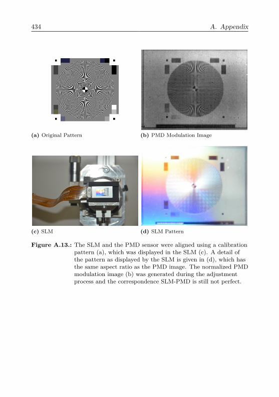
Calibration Pattern Test In order to achieve a perfect alignment betweenSLM and PMD sensor, a calibration pattern is displayed in the SLM andthe output of the PMD camera is visualized. The fine-adjustment screws ofthe SLM mount are then manually adjusted until the SLM pattern perfectlyfits the active area of the PMD array. An intermediate result of the processis given in Fig. A.13.The size of the calibration pattern (Fig. A.13a) is 1200 × 1600 and is

displayed by the SLM at full resolution. Fig. A.13c was acquired with aDSLR camera equipped with a linear polarizer, which was oriented as thepolarizer integrated in the telephot lens. Therefore, the detail in Fig. A.13dis just a high resolution image of what the PMD camera sees. The resolutionof the PMD sensor is ten times lower than that of the SLM. Consequently,the highest spatial frequencies of the pattern are lost in Fig. A.13b, whichprovides the PMD modulation image (amplitude of the modulated light)after normalization. Fig. A.13b was obtained directly from PMD raw data,without any processing.

434 A. Appendix

(a) Original Pattern (b) PMD Modulation Image

(c) SLM (d) SLM Pattern

Figure A.13.: The SLM and the PMD sensor were aligned using a calibrationpattern (a), which was displayed in the SLM (c). A detail ofthe pattern as displayed by the SLM is given in (d), which hasthe same aspect ratio as the PMD image. The normalized PMDmodulation image (b) was generated during the adjustmentprocess and the correspondence SLM-PMD is still not perfect.

A.12. Depth Measurement Uncertainty in the CS-PMD System 435

A.12. Depth Measurement Uncertainty in theCS-PMD System

In this section we derive Eq. 5.12 from Eq. 5.8 by error propagation. Forcompleteness, we first rewrite Eq. 5.8, which calculates the (ambiguous)depth for a single frequency (fi) from its two coefficients xsin

fi, xcosfi

:

di = dui

2π arctan(xsinfi

xcosfi

)− d0

i

dui = c

2fi

For further information, see Section 5.3.2. For simplicity, we operate inphase domain, where the previous equation can be rewritten as:

tan (θi − θ0i ) =

xsinfi

xcosfi

(A.13)

Similarly to Appendix A.4, we now apply the variance formula for uncer-tainty propagation, which reads

∆θi =

√√√√( δθiδxsinfi

)2

∆2xsinfi

+(

δθiδxcosfi

)2

∆2xcosfi

(A.14)

Both partial derivatives in Eq. A.14 can be easily calculated by differenti-ating Eq. A.13. We first differentiate with respect to xsin

fi. The phase offset

θ0i can be left away, since it does not affect the partial derivatives.

δ(tan θi)δθi

δθiδxsinfi

= 1xcosfi

1cos2 θi

δθiδxsinfi

= 1xcosfi

δθiδxsinfi

= 1xcosfi

cos2 θi

δθiδxsinfi

= 1xcosfi

(xcosfi

)2

(xcosfi

)2 + (xcosfi

)2 =xcosfi

(xcosfi

)2 + (xcosfi

)2

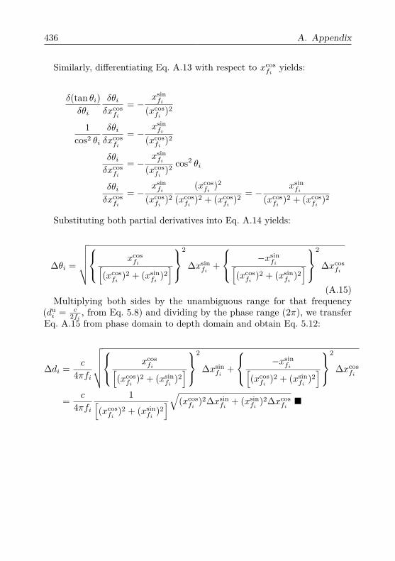
436 A. Appendix

Similarly, differentiating Eq. A.13 with respect to xcosfi

yields:

δ(tan θi)δθi

δθiδxcosfi

= −xsinfi

(xcosfi

)2

1cos2 θi

δθiδxcosfi

= −xsinfi

(xcosfi

)2

δθiδxcosfi

= −xsinfi

(xcosfi

)2 cos2 θi

δθiδxcosfi

= −xsinfi

(xcosfi

)2

(xcosfi

)2

(xcosfi

)2 + (xcosfi

)2 = −xsinfi

(xcosfi

)2 + (xcosfi

)2

Substituting both partial derivatives into Eq. A.14 yields:

∆θi =

√√√√√ xcos

fi[(xcosfi

)2 + (xsinfi

)2]

2

∆xsinfi

+

−xsinfi[

(xcosfi

)2 + (xsinfi

)2]

2

∆xcosfi

(A.15)Multiplying both sides by the unambiguous range for that frequency

(dui = c

2fi , from Eq. 5.8) and dividing by the phase range (2π), we transferEq. A.15 from phase domain to depth domain and obtain Eq. 5.12:

∆di = c

4πfi

√√√√√ xcos

fi[(xcosfi

)2 + (xsinfi

)2]

2

∆xsinfi

+

−xsinfi[

(xcosfi

)2 + (xsinfi

)2]

2

∆xcosfi

= c

4πfi1[

(xcosfi

)2 + (xsinfi

)2]√(xcos

fi)2∆xsin

fi+ (xsin

fi)2∆xcos

fi

References[1] 3D Image Sensor D-IMager. https://www.panasonic-electric-

works.com/eu-asset/pl/downloads/ds_dimager_flyer_en.pdf.[Online; accessed 06-May-2016]. 2010.

[2] J. B. Abbiss and W. T. Mayo. “Deviation-free Bragg cell frequency-shifting”. In: Appl. Opt. 20.4 (Feb. 1981), pp. 588–553. doi: 10.1364/AO.20.000588. url: http://ao.osa.org/abstract.cfm?URI=ao-20-4-588.

[3] M. Abolbashari, G. Babaie, F. Magalhães, M. V. Correia, F. M.Araújo, A. S. Gerges, and F. Farahi. “Biological imaging with highdynamic range using compressive imaging technique”. In: vol. 8225.2012, pp. 82251X–82251X–7. doi: 10.1117/12.907365. url: http://dx.doi.org/10.1117/12.907365.

[4] M. Abolbashari, F. Magalhães, F. M. M. Araújo, M. V. Correia,and F. Farahi. “High dynamic range compressive imaging: a pro-grammable imaging system”. In: Optical Engineering 51.7 (2012),pp. 071407–1–071407–8. doi: 10.1117/1.OE.51.7.071407. url:http://dx.doi.org/10.1117/1.OE.51.7.071407.

[5] D. Achlioptas. “Database-friendly Random Projections: Johnson-Lindenstrauss with Binary Coins”. In: J. Comput. Syst. Sci. 66.4(June 2003), pp. 671–687. issn: 0022-0000. doi: 10.1016/S0022-0000(03)00025-4. url: http://dx.doi.org/10.1016/S0022-0000(03)00025-4.

[6] M. Aharon, M. Elad, and A. Bruckstein. “K -SVD: An Algorithm forDesigning Overcomplete Dictionaries for Sparse Representation”. In:IEEE Transactions on Signal Processing 54.11 (Nov. 2006), pp. 4311–4322. issn: 1053-587X. doi: 10.1109/TSP.2006.881199.

[7] M. Aharon and M. Elad. “Sparse and Redundant Modeling of ImageContent Using an Image-Signature-Dictionary”. In: SIAM Journal onImaging Sciences 1.3 (2008), pp. 228–247. doi: 10.1137/07070156X.eprint: http://dx.doi.org/10.1137/07070156X. url: http://dx.doi.org/10.1137/07070156X.

© Springer Fachmedien Wiesbaden GmbH 2017M. Heredia Conde, Compressive Sensing for the Photonic MixerDevice, DOI 10.1007/978-3-658-18057-7

438 References

[8] N. Ahmed, T. Natarajan, and K. R. Rao. “Discrete Cosine Trans-form”. In: IEEE Transactions on Computers C-23.1 (Jan. 1974),pp. 90–93. issn: 0018-9340. doi: 10.1109/T-C.1974.223784.

[9] O. K. Al-Shaykh, I. Moccagatta, and H. Chen. “JPEG-2000: anew still image compression standard”. In: Signals, Systems amp;Computers, 1998. Conference Record of the Thirty-Second AsilomarConference on. Vol. 1. Nov. 1998, 99–103 vol.1. doi: 10.1109/ACSSC.1998.750835.

[10] M. A. Albota, R. M. Heinrichs, D. G. Kocher, D. G. Fouche, B. E.Player, M. E. O’Brien, B. F. Aull, J. J. Zayhowski, J. Mooney, B. C.Willard, and R. R. Carlson. “Three-dimensional imaging laser radarwith a photon-counting avalanche photodiode array and microchiplaser”. In: Appl. Opt. 41.36 (Dec. 2002), pp. 7671–7678. doi: 10.1364/AO.41.007671. url: http://ao.osa.org/abstract.cfm?URI=ao-41-36-7671.

[11] M. Albrecht. “Untersuchung von Photogate-PMD-Sensorenhinsichtlich qualifizierender Charakterisierungsparameter und-methoden”. PhD thesis. Siegen, Germany: Department of ElectricalEngineering and Computer Science, 2007, p. 229.

[12] J. B. Allen and L. R. Rabiner. “A unified approach to short-timeFourier analysis and synthesis”. In: Proceedings of the IEEE 65.11(Nov. 1977), pp. 1558–1564. issn: 0018-9219. doi: 10.1109/PROC.1977.10770.

[13] F. J. Anscombe. “The Transformation of Poisson, Binomial, andNegative-Binomial Data”. In: Biometrika 35.3/4 (1948), pp. 246–254.issn: 00063444. doi: 10.2307/2332343. url: http://dx.doi.org/10.2307/2332343.

[14] K. J. Arrow, L. Hurwicz, and H. Uzawa. Studies in linear and non-linear programming. Stanford Math. Stud. Social Sci. Stanford, CA:Cambridge Univ. Press, 1958.

[15] G. A. Atkinson and E. R. Hancock. “Recovery of surface orienta-tion from diffuse polarization”. In: IEEE Transactions on ImageProcessing 15.6 (June 2006), pp. 1653–1664. issn: 1057-7149. doi:10.1109/TIP.2006.871114.

[16] T. Azuma and A. Morimura. “Image Composite Method and ImageComposite Device”. Pat. 1996-154201. June 1996.

References 439

[17] R. Balan, P. Casazza, and Z. Landau. “Redundancy for localizedframes”. In: Israel Journal of Mathematics 185.1 (2011), pp. 445–476. issn: 1565-8511. doi: 10.1007/s11856- 011- 0118- 1. url:http://dx.doi.org/10.1007/s11856-011-0118-1.

[18] R. H. Bamberger and M. J. T. Smith. “A filter bank for the directionaldecomposition of images: theory and design”. In: IEEE Transactionson Signal Processing 40.4 (Apr. 1992), pp. 882–893. issn: 1053-587X.doi: 10.1109/78.127960.

[19] C. Bamji. “CMOS-compatible three-dimensional image sensor IC”.Pat. US Patent 6,323,942. Nov. 2001. url: http://www.google.com/patents/US6323942.

[20] C. Bamji and E. Charbon. “Systems for CMOS-compatible three-dimensional image sensing using quantum efficiency modulation”.Pat. US Patent 6,580,496. June 2003. url: http://www.google.com/patents/US6580496.

[21] C. Bamji, H. Yalcin, X. Liu, and E. Eroglu. “Method and systemto differentially enhance sensor dynamic range”. Pat. US Patent6,919,549. July 2005. url: http : / / www . google . de / patents /US6919549.

[22] C. S. Bamji, P. O’Connor, T. Elkhatib, S. Mehta, B. Thompson, L. A.Prather, D. Snow, O. C. Akkaya, A. Daniel, A. D. Payne, T. Perry,M. Fenton, and V. H. Chan. “A 0.13 µm CMOS System-on-Chipfor a 512 × 424 Time-of-Flight Image Sensor With Multi-FrequencyPhoto-Demodulation up to 130 MHz and 2 GS/s ADC”. In: IEEEJournal of Solid-State Circuits 50.1 (Jan. 2015), pp. 303–319. issn:0018-9200. doi: 10.1109/JSSC.2014.2364270.

[23] R. Bamler and P. Hartl. “Synthetic Aperture Radar Interferometry”.In: Inverse Problems 14 (Aug. 1998), pp. 1–54. doi: 10.1088/0266-5611/14/4/001. url: http://iopscience.iop.org/article/10.1088/0266-5611/14/4/001.

[24] R. Baraniuk. “Compressive Sensing [Lecture Notes]”. In: SignalProcessing Magazine, IEEE 24.4 (July 2007), pp. 118–121. issn:1053-5888. doi: 10.1109/MSP.2007.4286571.

[25] R. Baraniuk, V. Cevher, M. Duarte, and C. Hegde. “Model-BasedCompressive Sensing”. In: Information Theory, IEEE Transactionson 56.4 (Apr. 2010), pp. 1982–2001. issn: 0018-9448. doi: 10.1109/TIT.2010.2040894.

440 References

[26] R. Baraniuk, M. Davenport, R. DeVore, and M. Wakin. “A SimpleProof of the Restricted Isometry Property for Random Matrices”.In: Constructive Approximation 28.3 (2008), pp. 253–263. issn: 1432-0940. doi: 10.1007/s00365-007-9003-x. url: http://dx.doi.org/10.1007/s00365-007-9003-x.

[27] N. P. Barnes and L. B. Petway. “Variation of the Verdet constant withtemperature of terbium gallium garnet”. In: J. Opt. Soc. Am. B 9.10(Oct. 1992), pp. 1912–1915. doi: 10.1364/JOSAB.9.001912. url:http://josab.osa.org/abstract.cfm?URI=josab-9-10-1912.

[28] R. Barrett, M. Berry, T. F. Chan, J. Demmel, J. Donato, J. Dongarra,V. Eijkhout, R. Pozo, C. Romine, and H. V. der Vorst. Templatesfor the Solution of Linear Systems: Building Blocks for IterativeMethods, 2nd Edition. Philadelphia, PA: SIAM, 1994.

[29] J. Barry, E. Lee, and D. Messerschmitt. “Stochastic Signal Process-ing”. English. In: Digital Communication. Springer US, 2004, pp. 57–111. isbn: 978-1-4613-4975-4. doi: 10.1007/978-1-4615-0227-2_3.url: http://dx.doi.org/10.1007/978-1-4615-0227-2_3.

[30] M. S. Bartlett. “The Square Root Transformation in Analysis ofVariance”. English. In: Supplement to the Journal of the RoyalStatistical Society 3.1 (1936), pp. 68–78. issn: 14666162. url: http://www.jstor.org/stable/2983678.

[31] Basler Lab Time-of-Flight Cameras. http://www.i2s-vision.fr/upload/BAS1409_ToF_EN_web.pdf. [Online; accessed 06-May-2016].2016.

[32] Basler Time-of-Flight Camera. http://s.baslerweb.com/media/documents/BAS1603_ToF_Brochure_EN_SAP0022_web2.pdf. [On-line; accessed 06-May-2016]. 2016.

[33] S. Battiato, A. Castorina, and M. Mancuso. “High Dynamic RangeImaging for Digital Still Camera: An Overview”. In: Journal ofElectronic Imaging 12.3 (2003), pp. 459–469. doi: 10 . 1117 / 1 .1580829. url: http://dx.doi.org/10.1117/1.1580829.

[34] P. W. Baumeister. “Optical Tunneling and Its Applications to OpticalFilters”. In: Appl. Opt. 6.5 (May 1967), pp. 897–905. doi: 10.1364/AO.6.000897. url: http://ao.osa.org/abstract.cfm?URI=ao-6-5-897.

References 441

[35] W. Becker. The Bh TCSPC Handbook: Time-correlated Single PhotonCounting Modules SPC-130, SPC-134, SPC-130 EM, SPC-134 EM,SPC-140, SPC-144, SPC-150, SPC-154, SPC-630, SPC-730, SPC-830 ; Simple-Tau Systems, SPCM Software, SPCImage Data Analysis.Becker et Hickl, 2012. url: http://www.becker-hickl.de/pdf/SPC-handbook-6ed-12-web.pdf.

[36] S. Beigpour, A. Kolb, and S. Kunz. “A Comprehensive Multi-Illuminant Dataset for Benchmarking of the Intrinsic Image Al-gorithms”. In: June 2015.

[37] Z. Ben-Haim and Y. C. Eldar. “Performance bounds for sparseestimation with random noise”. In: Statistical Signal Processing,2009. SSP ’09. IEEE/SP 15th Workshop on. Aug. 2009, pp. 225–228.doi: 10.1109/SSP.2009.5278597.

[38] Z. Ben-Haim and Y. C. Eldar. “The Cramèr-Rao Bound for Estimat-ing a Sparse Parameter Vector”. In: IEEE Transactions on SignalProcessing 58.6 (June 2010), pp. 3384–3389. issn: 1053-587X. doi:10.1109/TSP.2010.2045423.

[39] Z. Ben-Haim, Y. C. Eldar, and M. Elad. “Coherence-Based Perfor-mance Guarantees for Estimating a Sparse Vector Under RandomNoise”. In: IEEE Transactions on Signal Processing 58.10 (Oct. 2010),pp. 5030–5043. issn: 1053-587X. doi: 10.1109/TSP.2010.2052460.

[40] J. J. Benedetto and M. Fickus. “Finite Normalized Tight Frames”.In: Advances in Computational Mathematics 18.2 (2003), pp. 357–385. issn: 1572-9044. doi: 10.1023/A:1021323312367. url: http://dx.doi.org/10.1023/A:1021323312367.

[41] A. Beurling. “Sur les intégrales de Fourier absolument convergenteset leur application à une transformation fonctionelle”. In: IX Congr.Math. Scand. Helsinki, Finland, 1938, pp. 345–366.

[42] G. Beylkin. “On the Representation of Operators in Bases of Com-pactly Supported Wavelets”. In: SIAM Journal on Numerical Anal-ysis 29.6 (1992), pp. 1716–1740. doi: 10.1137/0729097. eprint:http://dx.doi.org/10.1137/0729097. url: http://dx.doi.org/10.1137/0729097.

[43] A. Bhandari, M. Feigin, S. Izadi, C. Rhemann, M. Schmidt, andR. Raskar. “Resolving multipath interference in Kinect: An inverseproblem approach”. In: SENSORS, 2014 IEEE. Nov. 2014, pp. 614–617. doi: 10.1109/ICSENS.2014.6985073.

442 References

[44] A. Bhandari, C. Barsi, and R. Raskar. “Blind and reference-freefluorescence lifetime estimation via consumer time-of-flight sensors”.In: Optica 2.11 (Nov. 2015), pp. 965–973. doi: 10.1364/OPTICA.2.000965. url: http://www.osapublishing.org/optica/abstract.cfm?URI=optica-2-11-965.

[45] A. Bhandari, A. Kadambi, R. Whyte, C. Barsi, M. Feigin, A. Dor-rington, and R. Raskar. “Resolving multipath interference in time-of-flight imaging via modulation frequency diversity and sparseregularization”. In: Opt. Lett. 39.6 (Mar. 2014), pp. 1705–1708. doi:10.1364/OL.39.001705. url: http://ol.osa.org/abstract.cfm?URI=ol-39-6-1705.

[46] A. Bhatti, ed. Stereo Vision. Janeza Trdine 9, 51000 Rijeka, Croatia:InTech, 2008. isbn: 978-953-7619-22-0. doi: 10.5772/5898. url:http://www.intechopen.com/books/stereo_vision.

[47] L. Binqiao, S. Zhongyan, and X. Jiangtao. “Wide dynamic rangeCMOS image sensor with in-pixel double-exposure and synthesis”.In: Journal of Semiconductors 31.5 (2010), p. 055002. url: http://stacks.iop.org/1674-4926/31/i=5/a=055002.

[48] J. R. Bitner, G. Ehrlich, and E. M. Reingold. “Efficient Generation ofthe Binary Reflected Gray Code and Its Applications”. In: Commun.ACM 19.9 (Sept. 1976), pp. 517–521. issn: 0001-0782. doi: 10.1145/360336.360343. url: http://doi.acm.org/10.1145/360336.360343.

[49] F. Blais, M. Picard, and G. Godin. “Accurate 3D acquisition offreely moving objects”. In: 3D Data Processing, Visualization andTransmission, 2004. 3DPVT 2004. Proceedings. 2nd InternationalSymposium on. Sept. 2004, pp. 422–429. doi: 10.1109/TDPVT.2004.1335269.

[50] J. D. Blanchard, M. Cermak, D. Hanle, and Y. Jing. “Greedy Algo-rithms for Joint Sparse Recovery”. In: IEEE Transactions on SignalProcessing 62.7 (Apr. 2014), pp. 1694–1704. issn: 1053-587X. doi:10.1109/TSP.2014.2301980.

[51] R. G. Bland. “New Finite Pivoting Rules for the Simplex Method”.In: Mathematics of Operations Research 2.2 (1977), pp. 103–107. doi:10.1287/moor.2.2.103. eprint: http://dx.doi.org/10.1287/moor.2.2.103. url: http://dx.doi.org/10.1287/moor.2.2.103.

References 443

[52] L. Blinov and V. Chigrinov. Electrooptic Effects in Liquid CrystalMaterials. Partially Ordered Systems. Springer New York, 1996.isbn: 9780387947082. url: http://www.springer.com/us/book/9780387947082.

[53] T. Blumensath and M. Davies. “Sparse and shift-Invariant repre-sentations of music”. In: IEEE Transactions on Audio, Speech, andLanguage Processing 14.1 (Jan. 2006), pp. 50–57. issn: 1558-7916.doi: 10.1109/TSA.2005.860346.

[54] T. Blumensath and M. E. Davies. “Gradient Pursuits”. In: IEEETransactions on Signal Processing 56.6 (June 2008), pp. 2370–2382.issn: 1053-587X. doi: 10.1109/TSP.2007.916124.

[55] T. Blumensath and M. E. Davies. “Sampling Theorems for SignalsFrom the Union of Finite-Dimensional Linear Subspaces”. In: IEEETransactions on Information Theory 55.4 (Apr. 2009), pp. 1872–1882.issn: 0018-9448. doi: 10.1109/TIT.2009.2013003.

[56] T. Blumensath and M. E. Davies. “Normalized Iterative Hard Thresh-olding: Guaranteed Stability and Performance”. In: IEEE Journalof Selected Topics in Signal Processing 4.2 (Apr. 2010), pp. 298–309.issn: 1932-4553. doi: 10.1109/JSTSP.2010.2042411.

[57] T. Blumensath and M. E. Davies. “Iterative Thresholding for SparseApproximations”. In: Journal of Fourier Analysis and Applications14.5 (2008), pp. 629–654. issn: 1531-5851. doi: 10.1007/s00041-008-9035-z. url: http://dx.doi.org/10.1007/s00041-008-9035-z.

[58] B. G. Bodmann and J. Haas. “Achieving the orthoplex bound and con-structing weighted complex projective 2-designs with Singer sets”. In:CoRR abs/1509.05333 (Sept. 2015). arXiv: 1509.05333 [math.FA].url: http://arxiv.org/abs/1509.05333.

[59] B. G. Bodmann, P. G. Casazza, and G. Kutyniok. “A quantitativenotion of redundancy for finite frames”. In: Applied and Compu-tational Harmonic Analysis 30.3 (2011), pp. 348 –362. issn: 1063-5203. doi: http://dx.doi.org/10.1016/j.acha.2010.09.004.url: http://www.sciencedirect.com/science/article/pii/S1063520310001090.

444 References

[60] W. Böhler, V. M. Bordas, and A. Marbs. “Investigating laser scanneraccuracy”. In: ed. by O. Atlan. Vol. 34. 5/C15. Antalya, Turkey: In-ternational Committee for Documentation of Cultural Heritage, Oct.2003, pp. 696–701. url: http://cipa.icomos.org/fileadmin/template/doc/antalya/189.pdf.

[61] W. Böhler and A. Marbs. “3D Scanning Instruments”. In: Proceedingsof the CIPA WG 6 International Workshop on Scanning for CulturalHeritage Recording. Corfu, Greece, Sept. 2002.

[62] R. W. Boyd. Nonlinear Optics, Third Edition. 3rd. Academic Press,2008. isbn: 0123694701, 9780123694706.

[63] J. Brenner and L. Cummings. “The Hadamard Maximum Determi-nant Problem”. English. In: The American Mathematical Monthly79.6 (1972), pp. 626–630. issn: 00029890. url: http://www.jstor.org/stable/2317092.

[64] J. Burg. “Maximum entropy spectral analysis”. PhD thesis. 1975.[65] J. Butters and J. Leendertz. “Speckle pattern and holographic tech-

niques in engineering metrology”. In: Optics & Laser Technology 3.1(1971), pp. 26 –30. issn: 0030-3992. doi: http://dx.doi.org/10.1016/S0030-3992(71)80007-5. url: http://www.sciencedirect.com/science/article/pii/S0030399271800075.

[66] B. Büttgen. Extending Time-of-flight Optical 3D-imaging to ExtremeOperating Conditions. Sierke, 2007. isbn: 9783933893925. url: http://d-nb.info/983752990.

[67] B. Büttgen, M.-A. El Mechat, F. Lustenberger, and P. Seitz.“Pseudonoise Optical Modulation for Real-Time 3-D Imaging WithMinimum Interference”. In: Circuits and Systems I: Regular Papers,IEEE Transactions on 54.10 (Oct. 2007), pp. 2109–2119. issn:1549-8328. doi: 10.1109/TCSI.2007.904598.

[68] B. Büttgen, F. Lustenberger, and P. Seitz. “Demodulation PixelBased on Static Drift Fields”. In: Electron Devices, IEEE Trans-actions on 53.11 (Nov. 2006), pp. 2741–2747. issn: 0018-9383. doi:10.1109/TED.2006.883669.

[69] B. Büttgen and P. Seitz. “Robust Optical Time-of-Flight RangeImaging Based on Smart Pixel Structures”. In: Circuits and SystemsI: Regular Papers, IEEE Transactions on 55.6 (July 2008), pp. 1512–1525. issn: 1549-8328. doi: 10.1109/TCSI.2008.916679.

References 445

[70] B. Büttgen, T. Oggier, R. Kaufmann, P. Seitz, and N. Blanc. “Demon-stration of a novel drift field pixel structure for the demodulation ofmodulated light waves with application in three-dimensional imagecapture”. In: Proc. SPIE. Vol. 5302. 2004, pp. 9–20. doi: 10.1117/12.525654. url: http://dx.doi.org/10.1117/12.525654.

[71] B. Büttgen, T. Oggier, M. Lehmann, R. Kaufmann, and F. Lusten-berger. “CCD/CMOS Lock-in pixel for range imaging: challenges,limitations and state-of-the-art”. In: In Proceedings of 1st RangeImaging Research Day at ETH. Sept. 2005, pp. 21–32.

[72] B. Büttgen, T. Oggier, M. Lehmann, R. Kaufmann, S. Neukom,M. Richter, M. Schweizer, D. Beyeler, R. Cook, C. Gimkiewicz, C.Urban, P. Metzler, P. Seitz, and F. Lustenberger. “High-speed andhigh-sensitive demodulation pixel for 3D imaging”. In: Proc. SPIE.Vol. 6056. 2006, pp. 605603–605603–12. doi: 10.1117/12.642305.url: http://dx.doi.org/10.1117/12.642305.

[73] P. L. Butzer, P. J. S. G. Ferreira, J. R. Higgins, S. Saitoh, G.Schmeisser, and R. L. Stens. “Interpolation and Sampling: ET Whit-taker, K. Ogura and Their Followers”. In: The journal of Fourier anal-ysis and applications 17.2 (2011), pp. 320–354. issn: 1069-5869. doi:10.1007/s00041-010-9131-8. url: http://publications.rwth-aachen.de/record/191884.

[74] B. Buxbaum, J. Frey, H. Kraft, T. MÖller, and Z. Xu. “TOF-Pixel und Verfahren zu dessen Betrieb”. Pat. DE Patent App.DE200,510,056,774. May 2005. url: http://www.google.com/patents/DE102005056774A1?cl=de.

[75] B. Buxbaum. Optische Laufzeitentfernungsmessung und CDMAauf Basis der PMD-Technologie mittels phasenvariabler PN-Modulation. German. Vol. 17. ZESS Forschungsberichte. Aachen,Germany: Shaker Verlag, 2002, p. 218. isbn: 3-8265-9805-9. url:http://www.shaker.de/de/content/catalogue/index.asp?lang=de&ID=6&category=102.

[76] B. Buxbaum, R. Schwarte, T. Ringbeck, M. Grothof, and X. Luan.“MSM-PMD as correlation receiver in a new 3D-ranging system”. In:Proc. SPIE. Vol. 4546. 2002, pp. 145–153. doi: 10.1117/12.453994.url: http://dx.doi.org/10.1117/12.453994.

446 References

[77] B. Buxbaum, R. Schwarte, T. Ringbeck, H.-G. Heinol, Z. Xu, J.Olk, W. Tai, Z. Zhang, and X. Luan. “A new approach in opticalbroadband communication systems: a high integrated optical phaselocked loop based on a mixing and correlating sensor, the PhotonicMixer Device (PMD)”. In: Proceedings / OPTO 98, InternationalerKongress und Fachausstellung für Optische Sensorik, Messtechnikund Elektronik, 18. - 20. Mai 1998, Kongresszentrum Erfurt. 1998,pp. 59 –64.

[78] E. J. Candès and T. Tao. “Decoding by Linear Programming”. In:IEEE Trans. Inf. Theor. 51.12 (Dec. 2005), pp. 4203–4215. issn:0018-9448. doi: 10.1109/TIT.2005.858979. url: http://dx.doi.org/10.1109/TIT.2005.858979.

[79] E. Candès, J. Romberg, and T. Tao. “Robust uncertainty princi-ples: exact signal reconstruction from highly incomplete frequencyinformation”. In: Information Theory, IEEE Transactions on 52.2(Feb. 2006), pp. 489–509. issn: 0018-9448. doi: 10.1109/TIT.2005.862083.

[80] E. Candès and M. Wakin. “An Introduction To Compressive Sam-pling”. In: Signal Processing Magazine, IEEE 25.2 (Mar. 2008),pp. 21–30. issn: 1053-5888. doi: 10.1109/MSP.2007.914731.

[81] E. Candès and J. Romberg. “Sparsity and incoherence in compressivesampling”. In: Inverse Problems 23.3 (June 2007), pp. 969–985. url:http://resolver.caltech.edu/CaltechAUTHORS:CANip07.

[82] E. J. Candès. “Compressive sampling”. In: Proceedings oh the Inter-national Congress of Mathematicians. Aug. 2006, pp. 1433–1452.

[83] E. J. Candès. “The restricted isometry property and its implicationsfor compressed sensing”. In: Comptes Rendus Mathematique 346.9-10(2008), pp. 589 –592. issn: 1631-073X. doi: http://dx.doi.org/10.1016/j.crma.2008.03.014. url: http://www.sciencedirect.com/science/article/pii/S1631073X08000964.

[84] E. J. Candès, L. Demanet, D. Donoho, and L. Ying. “Fast DiscreteCurvelet Transforms”. In: Multiscale Modeling & Simulation 5.3(2006), pp. 861–899. doi: 10.1137/05064182X. eprint: http://dx.doi.org/10.1137/05064182X. url: http://dx.doi.org/10.1137/05064182X.

References 447

[85] E. J. Candès and D. L. Donoho. “Ridgelets: a key to higher-dimensional intermittency?” In: Philosophical Transactions ofthe Royal Society of London A: Mathematical, Physical andEngineering Sciences 357.1760 (1999), pp. 2495–2509. issn:1364-503X. doi: 10 . 1098 / rsta . 1999 . 0444. eprint: http ://rsta.royalsocietypublishing.org/content/357/1760/2495.full.pdf. url: http://rsta.royalsocietypublishing.org/content/357/1760/2495.

[86] E. J. Candès, Y. C. Eldar, D. Needell, and P. Randall. “Compressedsensing with coherent and redundant dictionaries”. In: Applied andComputational Harmonic Analysis 31.1 (2011), pp. 59 –73. issn: 1063-5203. doi: http://dx.doi.org/10.1016/j.acha.2010.10.002.url: http://www.sciencedirect.com/science/article/pii/S1063520310001156.

[87] E. J. Candès and Y. Plan. “Near-ideal model selection by l1 mini-mization”. In: Ann. Statist. 37.5A (Oct. 2009), pp. 2145–2177. doi:10.1214/08- AOS653. url: http://dx.doi.org/10.1214/08-AOS653.

[88] E. J. Candès and J. Romberg. “Robust Signal Recovery from Incom-plete Observations”. In: Image Processing, 2006 IEEE InternationalConference on. Oct. 2006, pp. 1281–1284. doi: 10.1109/ICIP.2006.312579.

[89] E. J. Candès and J. Romberg. l1-magic: Recovery of Sparse Signalsvia Convex Programming. 2005.

[90] E. J. Candès and J. Romberg. “Quantitative Robust UncertaintyPrinciples and Optimally Sparse Decompositions”. In: Found. Com-put. Math. 6.2 (Apr. 2006), pp. 227–254. issn: 1615-3375. doi:10.1007/s10208- 004- 0162- x. url: http://dx.doi.org/10.1007/s10208-004-0162-x.

[91] E. J. Candès, J. K. Romberg, and T. Tao. “Stable signal recoveryfrom incomplete and inaccurate measurements”. In: Communicationson Pure and Applied Mathematics 59.8 (2006), pp. 1207–1223. issn:1097-0312. doi: 10.1002/cpa.20124. url: http://dx.doi.org/10.1002/cpa.20124.

[92] E. J. Candès and T. Tao. “Near-Optimal Signal Recovery FromRandom Projections: Universal Encoding Strategies?” In: IEEETransactions on Information Theory 52.12 (Dec. 2006), pp. 5406–5425. issn: 0018-9448. doi: 10.1109/TIT.2006.885507.

448 References

[93] E. J. Candès and T. Tao. “The Dantzig selector: Statistical estimationwhen p is much larger than n”. In: Ann. Statist. 35.6 (Dec. 2007),pp. 2313–2351. doi: 10.1214/009053606000001523. url: http://dx.doi.org/10.1214/009053606000001523.

[94] E. J. Candès. “Ridgelets: theory and applications”. PhD thesis.Department of Statistics, Stanford University, 1998.

[95] C. Carathéodory. “Über den Variabilitätsbereich der Koeffizien-ten von Potenzreihen, die gegebene Werte nicht annehmen”. In:Mathematische Annalen 64.1 (1907), pp. 95–115. issn: 1432-1807.doi: 10.1007/BF01449883. url: http://dx.doi.org/10.1007/BF01449883.

[96] C. Carathéodory. “Über den variabilitätsbereich der fourier’schenkonstanten von positiven harmonischen funktionen”. In: Rendicontidel Circolo Matematico di Palermo (1884-1940) 32.1 (1911), pp. 193–217. issn: 0009-725X. doi: 10.1007/BF03014795. url: http://dx.doi.org/10.1007/BF03014795.

[97] D. Caspi, N. Kiryati, and J. Shamir. “Range imaging with adaptivecolor structured light”. In: Pattern Analysis and Machine Intelligence,IEEE Transactions on 20.5 (May 1998), pp. 470–480. issn: 0162-8828.doi: 10.1109/34.682177.

[98] A. Chambolle and T. Pock. “A First-Order Primal-Dual Algorithmfor Convex Problems with Applications to Imaging”. In: J. Math.Imaging Vis. 40.1 (May 2011), pp. 120–145. issn: 0924-9907. doi:10.1007/s10851- 010- 0251- 1. url: http://dx.doi.org/10.1007/s10851-010-0251-1.

[99] V. Chandar. A negative result concerning explicit matrices with therestricted isometry property. Tech. rep. 2008.

[100] V. Chandrasekaran, M. B. Wakin, D. Baron, and R. G. Baraniuk.“Surflets: a sparse representation for multidimensional functionscontaining smooth discontinuities”. In: Information Theory, 2004.ISIT 2004. Proceedings. International Symposium on. June 2004,pp. 563–. doi: 10.1109/ISIT.2004.1365602.

[101] V. Chandrasekaran, M. B. Wakin, D. Baron, and R. G. Baraniuk.“Representation and Compression of Multidimensional PiecewiseFunctions Using Surflets”. In: IEEE Transactions on InformationTheory 55.1 (Jan. 2009), pp. 374–400. issn: 0018-9448. doi: 10.1109/TIT.2008.2008153.

References 449

[102] E. Charbon. “Techniques for CMOS single photon imaging andprocessing”. In: ASIC, 2005. ASICON 2005. 6th International Con-ference On. Vol. 1. Oct. 2005, pp. 1163–1168. doi: 10.1109/ICASIC.2005.1611239.

[103] E. Charbon, H.-J. Yoon, and Y. Maruyama. “A Geiger mode APDfabricated in standard 65nm CMOS technology”. In: Electron DevicesMeeting (IEDM), 2013 IEEE International. Dec. 2013, pp. 27.5.1–27.5.4. doi: 10.1109/IEDM.2013.6724705.

[104] R. Chartrand. “Exact Reconstruction of Sparse Signals via Non-convex Minimization”. In: IEEE Signal Processing Letters 14.10(Oct. 2007), pp. 707–710. issn: 1070-9908. doi: 10.1109/LSP.2007.898300.

[105] R. Chartrand and W. Yin. “Iteratively reweighted algorithms forcompressive sensing”. In: 2008 IEEE International Conference onAcoustics, Speech and Signal Processing. Mar. 2008, pp. 3869–3872.doi: 10.1109/ICASSP.2008.4518498.

[106] J. Chen and X. Huo. “Theoretical Results on Sparse Representationsof Multiple-Measurement Vectors”. In: Signal Processing, IEEETransactions on 54.12 (Dec. 2006), pp. 4634–4643. issn: 1053-587X.doi: 10.1109/TSP.2006.881263.

[107] S. Chen, S. A. Billings, and W. Luo. “Orthogonal least squaresmethods and their application to non-linear system identification”.In: International Journal of Control 50.5 (1989). Address: London,pp. 1873–1896. url: http://eprints.soton.ac.uk/251147/.

[108] S. S. Chen, D. L. Donoho, and M. A. Saunders. “Atomic decomposi-tion by basis pursuit”. In: SIAM Journal on Scientific Computing20 (1998), pp. 33–61.

[109] N. Chenouard and M. Unser. “Learning Steerable Wavelet Frames”.In: Proceedings of the Ninth International Workshop on SamplingTheory and Applications (SampTA’11). Singapore, Republic of Sin-gapore: SampTA, May 2011. url: http : / / bigwww . epfl . ch /publications/chenouard1102.pdf.

[110] V. Cheung, B. J. Frey, and N. Jojic. “Video epitomes”. In: 2005IEEE Computer Society Conference on Computer Vision and PatternRecognition (CVPR’05). Vol. 1. June 2005, pp. 42–49. doi: 10.1109/CVPR.2005.366.

450 References

[111] A. Cohen, W. Dahmen, and R. Devore. “Compressed sensing andbest k-term approximation”. In: J. Amer. Math. Soc (2009), pp. 211–231.

[112] A. Cohen, R. DeVore, P. Petrushev, and H. Xu. “Nonlinear approxi-mation and the space BV(R2)”. In: American Journal of Mathematics121 (1999), pp. 587–628. doi: 10.1353/ajm.1999.0016.

[113] R. Coifman, F. Geshwind, and Y. Meyer. “Noiselets”. In: Appliedand Computational Harmonic Analysis 10.1 (2001), pp. 27 –44. issn:1063-5203. doi: http://dx.doi.org/10.1006/acha.2000.0313.url: http://www.sciencedirect.com/science/article/pii/S1063520300903130.

[114] R. R. Coifman and M. V. Wickerhauser. “Entropy-based algorithmsfor best basis selection”. In: IEEE Transactions on InformationTheory 38.2 (Mar. 1992), pp. 713–718. issn: 0018-9448. doi: 10.1109/18.119732.

[115] A. Colaço, A. Kirmani, G. Howland, J. Howell, and V. Goyal. “Com-pressive depth map acquisition using a single photon-counting de-tector: Parametric signal processing meets sparsity”. In: ComputerVision and Pattern Recognition (CVPR), 2012 IEEE Conference on.June 2012, pp. 96–102. doi: 10.1109/CVPR.2012.6247663.

[116] N. Collings, W. A. Crossland, P. J. Ayliffe, D. G. Vass, and I. Under-wood. “Evolutionary development of advanced liquid crystal spatiallight modulators”. In: Appl. Opt. 28.22 (Nov. 1989), pp. 4740–4747.doi: 10.1364/AO.28.004740. url: http://ao.osa.org/abstract.cfm?URI=ao-28-22-4740.

[117] R. M. Conroy, A. A. Dorrington, R. Künnemeyer, and M. J. Cree.“Range imager performance comparison in homodyne and heterodyneoperating modes”. In: Proc. SPIE. Vol. 7239. 2009, pp. 723905–723905–10. doi: 10.1117/12.806139. url: http://dx.doi.org/10.1117/12.806139.

[118] J. H. Conway, N. J. A. Sloane, and E. Bannai. Sphere-packings,Lattices, and Groups. New York, NY, USA: Springer-Verlag NewYork, Inc., 1987. isbn: 0-387-96617-X.

[119] J. Cooley and J. Tukey. “An Algorithm for the Machine Calculationof Complex Fourier Series”. In: Mathematics of Computation 19.90(1965), pp. 297–301.

References 451

[120] S. F. Cotter, B. D. Rao, K. Engan, and K. Kreutz-Delgado. “Sparsesolutions to linear inverse problems with multiple measurementvectors”. In: IEEE Transactions on Signal Processing 53.7 (July2005), pp. 2477–2488. issn: 1053-587X. doi: 10.1109/TSP.2005.849172.

[121] Cotton, A. and Mouton, H. “Sur la biréfringence magnétique desliquides purs. Comparaison avec le phénomène électro-optique deKerr”. In: J. Phys. Theor. Appl. 1.1 (1911), pp. 5–52. doi: 10.1051/jphystap:01911001010500. url: http://dx.doi.org/10.1051/jphystap:01911001010500.

[122] R. Craigen and J. Jedwab. Comment on "The Hadamard circulantconjecture". Tech. rep. arXiv:1111.3437. Nov. 2011. url: http://cds.cern.ch/record/1399299.

[123] M. S. Crouse, R. D. Nowak, and R. G. Baraniuk. “Wavelet-basedstatistical signal processing using hidden Markov models”. In: IEEETransactions on Signal Processing 46.4 (Apr. 1998), pp. 886–902.issn: 1053-587X. doi: 10.1109/78.668544.

[124] W. Dai and O. Milenkovic. “Subspace Pursuit for CompressiveSensing Signal Reconstruction”. In: IEEE Transactions on Informa-tion Theory 55.5 (May 2009), pp. 2230–2249. issn: 0018-9448. doi:10.1109/TIT.2009.2016006.

[125] G. B. Dantzig and M. N. Thapa. Linear Programming 1: Introduction.Secaucus, NJ, USA: Springer-Verlag New York, Inc., 1997. isbn: 0-387-94833-3.

[126] S. Das and N. Ahuja. “Active stereo based surface reconstruction”. In:Intelligent Control, 1990. Proceedingsof the 5th IEEE InternationalSymposium on. Vol. 1. Sept. 1990, pp. 233–238. doi: 10.1109/ISIC.1990.128463.

[127] S. Dasgupta and A. Gupta. “An elementary proof of a theorem ofJohnson and Lindenstrauss”. In: Random Structures & Algorithms22.1 (2003), pp. 60–65. issn: 1098-2418. doi: 10.1002/rsa.10073.url: http://dx.doi.org/10.1002/rsa.10073.

[128] I. Daubechies. “The wavelet transform, time-frequency localizationand signal analysis”. In: IEEE Transactions on Information Theory36.5 (Sept. 1990), pp. 961–1005. issn: 0018-9448. doi: 10.1109/18.57199.

452 References

[129] I. Daubechies. Ten Lectures on Wavelets. Society for Industrial andApplied Mathematics, 1992. doi: 10 . 1137 / 1 . 9781611970104.eprint: http : / / epubs . siam . org / doi / pdf / 10 . 1137 / 1 .9781611970104. url: http : / / epubs . siam . org / doi / abs / 10 .1137/1.9781611970104.

[130] I. Daubechies. “Orthonormal bases of compactly supported wavelets”.In: Communications on Pure and Applied Mathematics 41.7 (1988),pp. 909–996. issn: 1097-0312. doi: 10.1002/cpa.3160410705. url:http://dx.doi.org/10.1002/cpa.3160410705.

[131] I. Daubechies, R. DeVore, M. Fornasier, and C. S. Güntürk. “Iter-atively reweighted least squares minimization for sparse recovery”.In: Communications on Pure and Applied Mathematics 63.1 (2010),pp. 1–38. issn: 1097-0312. doi: 10.1002/cpa.20303. url: http://dx.doi.org/10.1002/cpa.20303.

[132] J. G. Daugman. “Complete discrete 2-D Gabor transforms by neuralnetworks for image analysis and compression”. In: IEEE Transac-tions on Acoustics, Speech, and Signal Processing 36.7 (July 1988),pp. 1169–1179. issn: 0096-3518. doi: 10.1109/29.1644.

[133] J. G. Daugman. “Two-dimensional spectral analysis of corticalreceptive field profiles”. In: Vision Research 20.10 (1980), pp. 847–856. issn: 0042-6989. doi: http://dx.doi.org/10.1016/0042-6989(80 ) 90065 - 6. url: http : / / www . sciencedirect . com /science/article/pii/0042698980900656.

[134] J. G. Daugman. “Uncertainty relation for resolution in space, spatialfrequency, and orientation optimized by two-dimensional visual cor-tical filters”. In: J. Opt. Soc. Am. A 2.7 (July 1985), pp. 1160–1169.doi: 10.1364/JOSAA.2.001160. url: http://josaa.osa.org/abstract.cfm?URI=josaa-2-7-1160.

[135] M. A. Davenport. “Random observations on random observations:Sparse signal acquisition and processing”. PhD thesis. Departmentof Electrical and Computer Engineering at Rice University, Aug.2010. url: http://dsp.rice.edu/sites/dsp.rice.edu/files/publications/thesis/2010/madphdthesis.pdf.

[136] M. Davidovic, M. Hofbauer, K. Schneider-Hornstein, and H. Zim-mermann. “High Dynamic Range Background Light Suppression fora TOF Distance Measurement Sensor in 180nm CMOS”. In: Sen-sors, 2011 IEEE. 2011, pp. 359–362. doi: 10.1109/ICSENS.2011.6127060.

References 453

[137] M. Davies and Y. Eldar. “Rank Awareness in Joint Sparse Recovery”.In: Information Theory, IEEE Transactions on 58.2 (Feb. 2012),pp. 1135–1146. issn: 0018-9448. doi: 10.1109/TIT.2011.2173722.

[138] P. E. Debevec and J. Malik. “Recovering High Dynamic RangeRadiance Maps from Photographs”. In: SIGGRAPH. 1997, pp. 369–378. url: http : / / dblp . uni - trier . de / db / conf / siggraph /siggraph1997.html#DebevecM97.

[139] P. Delsarte, J. Goethals, and J. Seidel. “Bounds for systems of lines,and Jacobi polynomials”. In: Philips Research Reports 30 (1975),pp. 91–105. issn: 0031-7918.

[140] P. B. Denyer, D. Renshaw, and S. Smith. “Intelligent CMOS imaging”.In: Proc. SPIE. Vol. 2415. 1995, pp. 285–291. doi: 10.1117/12.206525. url: http://dx.doi.org/10.1117/12.206525.

[141] R. A. DeVore. “Nonlinear Approximation”. In: Acta Numerica 7(1998), pp. 51–150.

[142] R. A. DeVore. “Deterministic constructions of compressed sensingmatrices”. In: Journal of Complexity 23.4-6 (2007). Festschrift forthe 60th Birthday of Henryk Woźniakowski, pp. 918–925. issn: 0885-064X. doi: http://dx.doi.org/10.1016/j.jco.2007.04.002.url: http://www.sciencedirect.com/science/article/pii/S0885064X07000623.

[143] A. Dib, N. Beaufort, and F. Charpillet. “A real time visual SLAMfor RGB-D cameras based on chamfer distance and occupancy grid”.In: International conference on advanced intelligent mechatronics.Besançon, France, July 2014, pp. 652 –657. doi: 10.1109/AIM.2014.6878153. url: https://hal.inria.fr/hal-01090998.

[144] A. G. Dimakis, R. Smarandache, and P. O. Vontobel. “LDPC Codesfor Compressed Sensing”. In: IEEE Transactions on InformationTheory 58.5 (May 2012), pp. 3093–3114. issn: 0018-9448. doi: 10.1109/TIT.2011.2181819.

[145] DMD 101: Introduction to Digital Micromirror Device (DMD) Tech-nology. http://www.ti.com/lit/an/dlpa008a/dlpa008a.pdf.[Online; accessed 26-August-2015]. 2013.

[146] M. N. Do and M. Vetterli. “The contourlet transform: an efficientdirectional multiresolution image representation”. In: IEEE Trans-actions on Image Processing 14.12 (Dec. 2005), pp. 2091–2106. issn:1057-7149. doi: 10.1109/TIP.2005.859376.

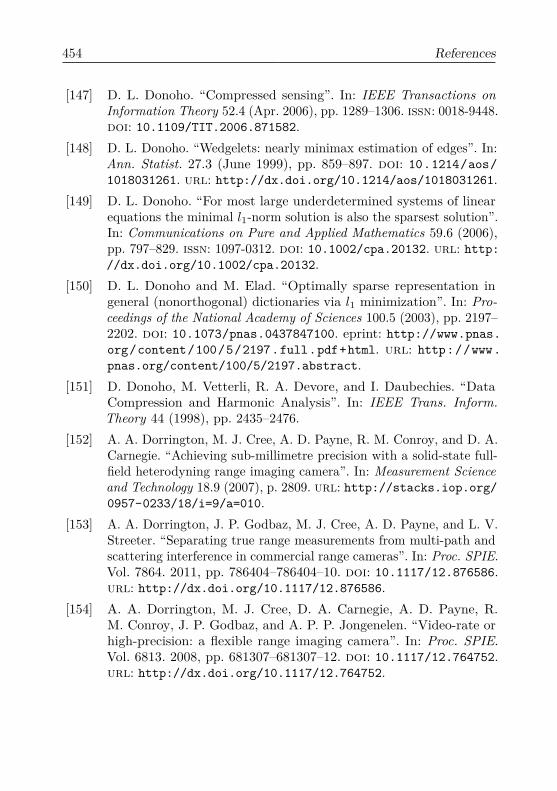
454 References

[147] D. L. Donoho. “Compressed sensing”. In: IEEE Transactions onInformation Theory 52.4 (Apr. 2006), pp. 1289–1306. issn: 0018-9448.doi: 10.1109/TIT.2006.871582.

[148] D. L. Donoho. “Wedgelets: nearly minimax estimation of edges”. In:Ann. Statist. 27.3 (June 1999), pp. 859–897. doi: 10.1214/aos/1018031261. url: http://dx.doi.org/10.1214/aos/1018031261.

[149] D. L. Donoho. “For most large underdetermined systems of linearequations the minimal l1-norm solution is also the sparsest solution”.In: Communications on Pure and Applied Mathematics 59.6 (2006),pp. 797–829. issn: 1097-0312. doi: 10.1002/cpa.20132. url: http://dx.doi.org/10.1002/cpa.20132.

[150] D. L. Donoho and M. Elad. “Optimally sparse representation ingeneral (nonorthogonal) dictionaries via l1 minimization”. In: Pro-ceedings of the National Academy of Sciences 100.5 (2003), pp. 2197–2202. doi: 10.1073/pnas.0437847100. eprint: http://www.pnas.org/content/100/5/2197.full.pdf+html. url: http://www.pnas.org/content/100/5/2197.abstract.

[151] D. Donoho, M. Vetterli, R. A. Devore, and I. Daubechies. “DataCompression and Harmonic Analysis”. In: IEEE Trans. Inform.Theory 44 (1998), pp. 2435–2476.

[152] A. A. Dorrington, M. J. Cree, A. D. Payne, R. M. Conroy, and D. A.Carnegie. “Achieving sub-millimetre precision with a solid-state full-field heterodyning range imaging camera”. In: Measurement Scienceand Technology 18.9 (2007), p. 2809. url: http://stacks.iop.org/0957-0233/18/i=9/a=010.

[153] A. A. Dorrington, J. P. Godbaz, M. J. Cree, A. D. Payne, and L. V.Streeter. “Separating true range measurements from multi-path andscattering interference in commercial range cameras”. In: Proc. SPIE.Vol. 7864. 2011, pp. 786404–786404–10. doi: 10.1117/12.876586.url: http://dx.doi.org/10.1117/12.876586.

[154] A. A. Dorrington, M. J. Cree, D. A. Carnegie, A. D. Payne, R.M. Conroy, J. P. Godbaz, and A. P. P. Jongenelen. “Video-rate orhigh-precision: a flexible range imaging camera”. In: Proc. SPIE.Vol. 6813. 2008, pp. 681307–681307–12. doi: 10.1117/12.764752.url: http://dx.doi.org/10.1117/12.764752.

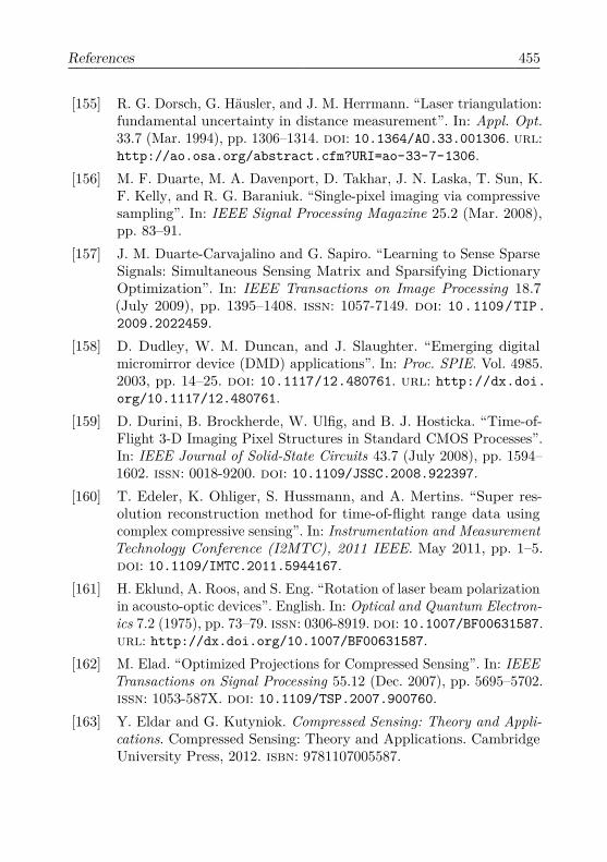
References 455

[155] R. G. Dorsch, G. Häusler, and J. M. Herrmann. “Laser triangulation:fundamental uncertainty in distance measurement”. In: Appl. Opt.33.7 (Mar. 1994), pp. 1306–1314. doi: 10.1364/AO.33.001306. url:http://ao.osa.org/abstract.cfm?URI=ao-33-7-1306.

[156] M. F. Duarte, M. A. Davenport, D. Takhar, J. N. Laska, T. Sun, K.F. Kelly, and R. G. Baraniuk. “Single-pixel imaging via compressivesampling”. In: IEEE Signal Processing Magazine 25.2 (Mar. 2008),pp. 83–91.

[157] J. M. Duarte-Carvajalino and G. Sapiro. “Learning to Sense SparseSignals: Simultaneous Sensing Matrix and Sparsifying DictionaryOptimization”. In: IEEE Transactions on Image Processing 18.7(July 2009), pp. 1395–1408. issn: 1057-7149. doi: 10.1109/TIP.2009.2022459.

[158] D. Dudley, W. M. Duncan, and J. Slaughter. “Emerging digitalmicromirror device (DMD) applications”. In: Proc. SPIE. Vol. 4985.2003, pp. 14–25. doi: 10.1117/12.480761. url: http://dx.doi.org/10.1117/12.480761.

[159] D. Durini, B. Brockherde, W. Ulfig, and B. J. Hosticka. “Time-of-Flight 3-D Imaging Pixel Structures in Standard CMOS Processes”.In: IEEE Journal of Solid-State Circuits 43.7 (July 2008), pp. 1594–1602. issn: 0018-9200. doi: 10.1109/JSSC.2008.922397.

[160] T. Edeler, K. Ohliger, S. Hussmann, and A. Mertins. “Super res-olution reconstruction method for time-of-flight range data usingcomplex compressive sensing”. In: Instrumentation and MeasurementTechnology Conference (I2MTC), 2011 IEEE. May 2011, pp. 1–5.doi: 10.1109/IMTC.2011.5944167.

[161] H. Eklund, A. Roos, and S. Eng. “Rotation of laser beam polarizationin acousto-optic devices”. English. In: Optical and Quantum Electron-ics 7.2 (1975), pp. 73–79. issn: 0306-8919. doi: 10.1007/BF00631587.url: http://dx.doi.org/10.1007/BF00631587.

[162] M. Elad. “Optimized Projections for Compressed Sensing”. In: IEEETransactions on Signal Processing 55.12 (Dec. 2007), pp. 5695–5702.issn: 1053-587X. doi: 10.1109/TSP.2007.900760.

[163] Y. Eldar and G. Kutyniok. Compressed Sensing: Theory and Appli-cations. Compressed Sensing: Theory and Applications. CambridgeUniversity Press, 2012. isbn: 9781107005587.

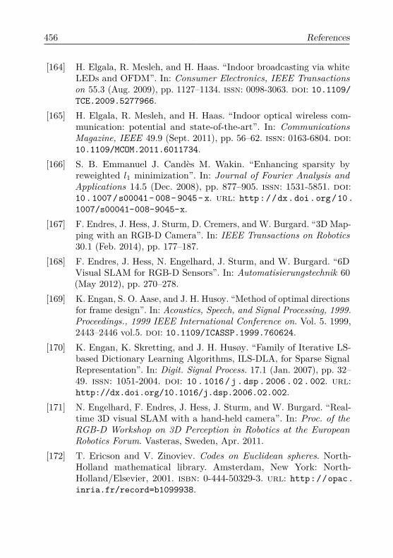
456 References

[164] H. Elgala, R. Mesleh, and H. Haas. “Indoor broadcasting via whiteLEDs and OFDM”. In: Consumer Electronics, IEEE Transactionson 55.3 (Aug. 2009), pp. 1127–1134. issn: 0098-3063. doi: 10.1109/TCE.2009.5277966.

[165] H. Elgala, R. Mesleh, and H. Haas. “Indoor optical wireless com-munication: potential and state-of-the-art”. In: CommunicationsMagazine, IEEE 49.9 (Sept. 2011), pp. 56–62. issn: 0163-6804. doi:10.1109/MCOM.2011.6011734.

[166] S. B. Emmanuel J. Candès M. Wakin. “Enhancing sparsity byreweighted l1 minimization”. In: Journal of Fourier Analysis andApplications 14.5 (Dec. 2008), pp. 877–905. issn: 1531-5851. doi:10.1007/s00041- 008- 9045- x. url: http://dx.doi.org/10.1007/s00041-008-9045-x.

[167] F. Endres, J. Hess, J. Sturm, D. Cremers, and W. Burgard. “3D Map-ping with an RGB-D Camera”. In: IEEE Transactions on Robotics30.1 (Feb. 2014), pp. 177–187.

[168] F. Endres, J. Hess, N. Engelhard, J. Sturm, and W. Burgard. “6DVisual SLAM for RGB-D Sensors”. In: Automatisierungstechnik 60(May 2012), pp. 270–278.

[169] K. Engan, S. O. Aase, and J. H. Husoy. “Method of optimal directionsfor frame design”. In: Acoustics, Speech, and Signal Processing, 1999.Proceedings., 1999 IEEE International Conference on. Vol. 5. 1999,2443–2446 vol.5. doi: 10.1109/ICASSP.1999.760624.

[170] K. Engan, K. Skretting, and J. H. Husøy. “Family of Iterative LS-based Dictionary Learning Algorithms, ILS-DLA, for Sparse SignalRepresentation”. In: Digit. Signal Process. 17.1 (Jan. 2007), pp. 32–49. issn: 1051-2004. doi: 10.1016/j.dsp.2006.02.002. url:http://dx.doi.org/10.1016/j.dsp.2006.02.002.

[171] N. Engelhard, F. Endres, J. Hess, J. Sturm, and W. Burgard. “Real-time 3D visual SLAM with a hand-held camera”. In: Proc. of theRGB-D Workshop on 3D Perception in Robotics at the EuropeanRobotics Forum. Vasteras, Sweden, Apr. 2011.

[172] T. Ericson and V. Zinoviev. Codes on Euclidean spheres. North-Holland mathematical library. Amsterdam, New York: North-Holland/Elsevier, 2001. isbn: 0-444-50329-3. url: http://opac.inria.fr/record=b1099938.

References 457

[173] A. Esposito, T. Oggier, H. Gerritsen, F. Lustenberger, andF. Wouters. “All-solid-state lock-in imaging for wide-field fluo-rescence lifetime sensing”. In: Opt. Express 13.24 (Nov. 2005),pp. 9812–9821. doi: 10 . 1364 / OPEX . 13 . 009812. url: http ://www.opticsexpress.org/abstract.cfm?URI=oe-13-24-9812.

[174] M. Fazel, H. Hindi, and S. P. Boyd. “Log-det heuristic for matrix rankminimization with applications to Hankel and Euclidean distancematrices”. In: American Control Conference. Vol. 3. 2003. doi: 10.1109/ACC.2003.1243393.

[175] P. Feng and Y. Bresler. “Spectrum-blind minimum-rate samplingand reconstruction of multiband signals”. In: Acoustics, Speech, andSignal Processing, 1996. ICASSP-96. Conference Proceedings., 1996IEEE International Conference on. Vol. 3. May 1996, 1688–1691 vol.3. doi: 10.1109/ICASSP.1996.544131.

[176] Fluorescence Lifetime Imaging - Application Simplified. http://www.pco.de/fileadmin/user_upload/pco-product_sheets/pco.flim_data_sheet.pdf. [Online; accessed 30-May-2016]. 2016.

[177] D. Fofi, T. Sliwa, and Y. Voisin. “A comparative survey on invisiblestructured light”. In: Proc. SPIE. Vol. 5303. 2004, pp. 90–98. doi: 10.1117/12.525369. url: http://dx.doi.org/10.1117/12.525369.

[178] A. Foi. Optimization of variance-stabilizing transformations. 2009.url: http://www.cs.tut.fi/~foi.

[179] S. Foix, G. Alenya, and C. Torras. “Lock-in Time-of-Flight(ToF) Cameras: A Survey”. In: Sensors Journal, IEEE 11.9 (2011),pp. 1917–1926. issn: 1530-437X. doi: 10.1109/JSEN.2010.2101060.

[180] M. Fornasier and H. Rauhut. “Compressive Sensing”. In: Handbookof Mathematical Methods in Imaging. Ed. by O. Scherzer. Springer,2011, pp. 187–228. doi: 10.1007/978-0-387-92920-0_6.

[181] A. Fossati, J. Gall, H. Grabner, X. Ren, and K. Konolige. ConsumerDepth Cameras for Computer Vision: Research Topics and Appli-cations. Springer Publishing Company, Incorporated, 2012. isbn:1447146395, 9781447146391.

[182] S. Foucart. “Hard Thresholding Pursuit: An Algorithm for Com-pressive Sensing”. In: SIAM Journal on Numerical Analysis 49.6(2011), pp. 2543–2563. doi: 10 . 1137 / 100806278. eprint: http ://dx.doi.org/10.1137/100806278. url: http://dx.doi.org/10.1137/100806278.

458 References

[183] S. Foucart, A. Pajor, H. Rauhut, and T. Ullrich. “The Gelfandwidths of -balls for”. In: Journal of Complexity 26.6 (2010), pp. 629–640. issn: 0885-064X. doi: http://dx.doi.org/10.1016/j.jco.2010.04.004. url: http://www.sciencedirect.com/science/article/pii/S0885064X10000282.

[184] S. Foucart and H. Rauhut. A Mathematical Introduction toCompressive Sensing. Birkhäuser Basel, 2013. isbn: 0817649476,9780817649470.

[185] J. E. Fowler. “The Redundant Discrete Wavelet Transform andAdditive Noise”. In: IEEE Signal Processing Letters 12.9 (2005),pp. 629–632. issn: 1070-9908. doi: 10.1109/LSP.2005.853048.

[186] M. Fox and R Ispasoiu. “Quantum wells, superlattices, and band-gap engineering”. In: Springer Handbook of Electronic and PhotonicMaterials. Ed. by S. Kasap and P. Capper. Springer Handbook ofElectronic and Photonic Materials. Springer, 2006, pp. 1021–1039.isbn: 9780387291857. url: https://books.google.de/books?id=rVVW22pnzhoC.

[187] G. Frank. “Verfahren und Vorrichtung zur Bestimmung vonProbeneigenschaften über zeitaufgelöste Lumineszenz”. Pat. DEPatent App. DE1,999,151,154. May 2001. url: http://www.google.com/patents/DE19951154A1?cl=de.

[188] B. Freedman, A. Shpunt, M. Machline, and Y. Arieli. “Depth map-ping using projected patterns”. Pat. US Patent App. 11/899,542. Oct.2008. url: http://www.google.com/patents/US20080240502.

[189] D. Freedman, Y. Smolin, E. Krupka, I. Leichter, and M. Schmidt.“SRA: Fast Removal of General Multipath for ToF Sensors”. English.In: Computer Vision – ECCV 2014. Ed. by D. Fleet, T. Pajdla, B.Schiele, and T. Tuytelaars. Vol. 8689. Lecture Notes in ComputerScience. Springer International Publishing, 2014, pp. 234–249. isbn:978-3-319-10589-5. doi: 10.1007/978-3-319-10590-1_16. url:http://dx.doi.org/10.1007/978-3-319-10590-1_16.

[190] M. F. Freeman and J. W. Tukey. “Transformations Related to theAngular and the Square Root”. In: Ann. Math. Statist. 21.4 (Dec.1950), pp. 607–611. doi: 10.1214/aoms/1177729756. url: http://dx.doi.org/10.1214/aoms/1177729756.

References 459

[191] K. P. F.R.S. “LIII. On lines and planes of closest fit to systems ofpoints in space”. In: Philosophical Magazine Series 6 2.11 (1901),pp. 559–572. doi: 10.1080/14786440109462720. eprint: http://dx.doi.org/10.1080/14786440109462720. url: http://dx.doi.org/10.1080/14786440109462720.

[192] S. Fuchs. “Multipath Interference Compensation in Time-of-FlightCamera Images”. In: Pattern Recognition (ICPR), 2010 20th Inter-national Conference on. Aug. 2010, pp. 3583–3586. doi: 10.1109/ICPR.2010.874.

[193] S. Fuchs, M. Suppa, and O. Hellwich. “Compensation for Multipathin ToF Camera Measurements Supported by Photometric Calibrationand Environment Integration”. English. In: Computer Vision Systems.Ed. by M. Chen, B. Leibe, and B. Neumann. Vol. 7963. Lecture Notesin Computer Science. Springer Berlin Heidelberg, 2013, pp. 31–41.isbn: 978-3-642-39401-0. doi: 10.1007/978-3-642-39402-7_4.url: http://dx.doi.org/10.1007/978-3-642-39402-7_4.

[194] D. Gabor. “Theory of communication. Part 1: The analysis of infor-mation”. In: Electrical Engineers - Part III: Radio and Communi-cation Engineering, Journal of the Institution of 93.26 (Nov. 1946),pp. 429–441. doi: 10.1049/ji-3-2.1946.0074.

[195] R. Gallager. “Low-density parity-check codes”. In: IRE Transactionson Information Theory 8.1 (Jan. 1962), pp. 21–28. issn: 0096-1000.doi: 10.1109/TIT.1962.1057683.

[196] R. G. Gallager. “Low-Density Parity-Check Codes”. PhD thesis.Cambridge MA, 1963.

[197] L. Gan, T. T. Do, and T. D. Tran. “Fast compressive imagingusing scrambled block Hadamard ensemble”. In: Signal ProcessingConference, 2008 16th European. Aug. 2008, pp. 1–5.

[198] L. Gao, J. Liang, C. Li, and L. V. Wang. “Single-shot compressedultrafast photography at one hundred billion frames per second”.In: Nature 516.7529 (Dec. 2014), pp. 74–77. issn: 0028-0836. doi:10.1038/nature14005. url: \urlhttp://dx.doi.org/10.1038/nature14005.

[199] S. Gautam and D. Vaintrob. A Novel Approach to the SphericalCodes Problem. Tech. rep. Massachusetts Institute of Technology,2012.

460 References

[200] S. A. Gersgorin. “Über die abgrenzung der eigenwerte einer Ma-trix”. In: Bulletin de l’Académie des Sciences de l’URSS. Classe desSciences Mathématiques et na 6 (1931), pp. 749–754. url: http://www.mathnet.ru/links/9372171f9b618598dad64a5ad1d40eef/im5235.pdf.

[201] A. C. Gilbert, S. Guha, P. Indyk, S. Muthukrishnan, and M. Strauss.“Near-optimal Sparse Fourier Representations via Sampling”. In:Proceedings of the Thiry-fourth Annual ACM Symposium on Theoryof Computing. STOC ’02. Montreal, Quebec, Canada: ACM, 2002,pp. 152–161. isbn: 1-58113-495-9. doi: 10.1145/509907.509933.url: http://doi.acm.org/10.1145/509907.509933.

[202] A. C. Gilbert, S. Muthukrishnan, and M. J. Strauss. “Approximationof Functions over Redundant Dictionaries Using Coherence”. In:Proceedings of the Fourteenth Annual ACM-SIAM Symposium onDiscrete Algorithms. SODA ’03. Baltimore, Maryland: Society forIndustrial and Applied Mathematics, 2003, pp. 243–252. isbn: 0-89871-538-5. url: http://www.math.lsa.umich.edu/~annacg/papers/GMS03.cat.pdf.

[203] J. P. Godbaz, M. J. Cree, and A. A. Dorrington. “Closed-form in-verses for the mixed pixel/multipath interference problem in AMCWlidar”. In: Proc. SPIE. Vol. 8296. 2012, pp. 829618–829618–15. doi:10.1117/12.909778. url: http://dx.doi.org/10.1117/12.909778.

[204] I. F. Gorodnitsky and B. D. Rao. “Sparse signal reconstructionfrom limited data using FOCUSS: a re-weighted minimum normalgorithm”. In: IEEE Transactions on Signal Processing 45.3 (Mar.1997), pp. 600–616. issn: 1053-587X. doi: 10.1109/78.558475.

[205] Y. Gousseau and J.-M. Morel. “Are Natural Images of BoundedVariation?” In: SIAM Journal on Mathematical Analysis 33.3 (2001),pp. 634–648. doi: 10.1137/S0036141000371150. eprint: http://dx.doi.org/10.1137/S0036141000371150. url: http://dx.doi.org/10.1137/S0036141000371150.

[206] J. E. Greivenkamp. “Generalized Data Reduction For HeterodyneInterferometry”. In: Optical Engineering 23.4 (1984), pp. 234350–234350–. doi: 10.1117/12.7973298. url: http://dx.doi.org/10.1117/12.7973298.

References 461

[207] R. Grosse, M. K. Johnson, E. H. Adelson, and W. T. Freeman.“Ground-truth dataset and baseline evaluations for intrinsic im-age algorithms”. In: International Conference on Computer Vision(ICCV). 2009, pp. 2335–2342. doi: http://dx.doi.org/10.1109/ICCV.2009.5459428.

[208] S. Guđmundsson, H. Aanæaes, and R. Larsen. “Environmental Ef-fects on Measurement Uncertainties of Time-of-Flight Cameras”.In: Signals, Circuits and Systems, 2007. ISSCS 2007. InternationalSymposium on. Vol. 1. July 2007, pp. 1–4. doi: 10.1109/ISSCS.2007.4292664.

[209] M. Gupta, S. K. Nayar, M. Hullin, and J. Martin. “Phasor Imaging:A Generalization Of Correlation-Based Time-of-Flight Imaging”. In:ACM Transactions on Graphics (TOG), presented at SIGGRAPH2015 34.5 (Oct. 2015).

[210] A. Haar. “Zur Theorie der orthogonalen Funktionensysteme”. In:Mathematische Annalen 69.3 (), pp. 331–371. issn: 1432-1807. doi:10 . 1007 / BF01456326. url: http : / / dx . doi . org / 10 . 1007 /BF01456326.

[211] J. Hadamard. “Résolution d’une question relative aux déterminants”.In: Bull. Sci. Math. 17 (1893), pp. 240–246.

[212] S. M. Han, T. Takasawa, K. Yasutomi, S. Aoyama, K. Kagawa, and S.Kawahito. “A Time-of-Flight Range Image Sensor With BackgroundCanceling Lock-in Pixels Based on Lateral Electric Field ChargeModulation”. In: IEEE Journal of the Electron Devices Society 3.3(May 2015), pp. 267–275. issn: 2168-6734. doi: 10.1109/JEDS.2014.2382689.

[213] M. Hansard, S. Lee, O. Choi, and R. Horaud. Time of Flight Cameras:Principles, Methods, and Applications. SpringerBriefs in ComputerScience. Springer, 2013.

[214] P. Hariharan. Optical Interferometry. Electronics & Electrical. Aca-demic Press, 2003. isbn: 9780123116307. url: https://books.google.de/books?id=EGdMO3rfVj4C.

[215] P. Hariharan. Basics of Interferometry. Elsevier Science, 2010. isbn:9780080465456. url: https://books.google.com.br/books?id=sWbGSSQ6fPYC.

462 References

[216] K. Hartmann and R. Schwarte. “Detection of the phase and ampli-tude of electromagnetic waves”. Pat. US7238927 B1. July 2007. url:https://www.google.com/patents/US7238927.

[217] J. Haupt, R. M. Castro, and R. Nowak. “Distilled Sensing: AdaptiveSampling for Sparse Detection and Estimation”. In: IEEE Transac-tions on Information Theory 57.9 (Sept. 2011), pp. 6222–6235. issn:0018-9448. doi: 10.1109/TIT.2011.2162269.

[218] Z. He, T. Ogawa, and M. Haseyama. “The simplest measurementmatrix for compressed sensing of natural images”. In: Image Pro-cessing (ICIP), 2010 17th IEEE International Conference on. Sept.2010, pp. 4301–4304. doi: 10.1109/ICIP.2010.5651800.

[219] A. Hedayat, N. J. A. N. J. A. Sloane, and J. Stufken. Orthogonalarrays : theory and applications. Springer series in statistics. NewYork: Springer, 1999. isbn: 0-387-98766-5. url: http://opac.inria.fr/record=b1097587.

[220] F. Heide, M. B. Hullin, J. Gregson, and W. Heidrich. “Low-budgetTransient Imaging Using Photonic Mixer Devices”. In: ACM Trans-actions on Graphics 32.4 (July 2013), 45:1–45:10. issn: 0730-0301.doi: 10.1145/2461912.2461945. url: http://doi.acm.org/10.1145/2461912.2461945.

[221] F. Heide, L. Xiao, A. Kolb, M. B. Hullin, and W. Heidrich. “Imagingin scattering media using correlation image sensors and sparse convo-lutional coding”. In: Opt. Express 22.21 (Oct. 2014), pp. 26338–26350.doi: 10.1364/OE.22.026338. url: http://www.opticsexpress.org/abstract.cfm?URI=oe-22-21-26338.

[222] H. G. Heinol. “Untersuchung und Entwicklung von modulation-slaufzeitbasierten 3D-Sichtsystemen”. German. PhD thesis. Siegen,Germany: Department of Electrical Engineering and Computer Sci-ence, 2001, p. 157.

[223] P. Henry, M. Krainin, E. Herbst, X. Ren, and D. Fox. “Rgbd mapping:Using depth cameras for dense 3d modeling of indoor environments”.In: In RGB-D: Advanced Reasoning with Depth Cameras Workshopin conjunction with RSS. 2010.

[224] High Definition Lidar HDL-64E S2. http://velodynelidar.com/lidar/products/brochure/HDL-64E%20S2%20datasheet_2010_lowres.pdf. [Online; accessed 27-July-2014]. 2014.

References 463

[225] B. Höfflinger. High-Dynamic-Range (HDR) Vision: Microelectronics,Image Processing, Computer Graphics (Springer Series in AdvancedMicroelectronics). Secaucus, NJ, USA: Springer-Verlag New York,Inc., 2007. isbn: 3540444327.

[226] H. A. Höfler, V. Jetter, and E. E. Wagner. “3D profiling by opticaldemodulation with an image intensifier”. In: Proc. SPIE. Vol. 3640.1999, pp. 21–27. doi: 10.1117/12.341068. url: http://dx.doi.org/10.1117/12.341068.

[227] E. Horn and N. Kiryati. “Toward optimal structured light patterns”.In: 3-D Digital Imaging and Modeling, 1997. Proceedings., Interna-tional Conference on Recent Advances in. May 1997, pp. 28–35. doi:10.1109/IM.1997.603845.

[228] J. P. Hornak. “The Basics of MRI”. 1996. url: http://www.cis.rit.edu/htbooks/mri/.

[229] L. Hornbeck. “Spatial light modulator and method”. Pat. US Patent5,061,049. Oct. 1991. url: http://www.google.com/patents/US5061049.

[230] G. A. Howland, D. J. Lum, M. R. Ware, and J. C. Howell. “Photoncounting compressive depth mapping”. In: CoRR abs/1309.4385(2013). url: http://arxiv.org/abs/1309.4385.

[231] X.-Y. Hu, E. Eleftheriou, and D. M. Arnold. “Progressive edge-growth Tanner graphs”. In: Global Telecommunications Conference,2001. GLOBECOM ’01. IEEE. Vol. 2. 2001, 995–1001 vol.2. doi:10.1109/GLOCOM.2001.965567.

[232] X.-Y. Hu, E. Eleftheriou, and D. M. Arnold. “Regular and irregularprogressive edge-growth tanner graphs”. In: IEEE Transactions onInformation Theory 51.1 (Jan. 2005), pp. 386–398. issn: 0018-9448.doi: 10.1109/TIT.2004.839541.

[233] A. S. Huang, A. Bachrach, P. Henry, M. Krainin, D. Fox, and N.Roy. “Visual odometry and mapping for autonomous flight using anRGB-D camera”. In: In Proc. of the Intl. Sym. of Robot. Research.2011.

[234] B. Hurley, P. Hurley, and T. Hurley. “The Hadamard circulant conjec-ture”. In: Bulletin of the London Mathematical Society (2011). doi:10.1112/blms/bdq112. eprint: http://blms.oxfordjournals.org/content/early/2011/01/24/blms.bdq112.full.pdf+html.

464 References

url: http://blms.oxfordjournals.org/content/early/2011/01/24/blms.bdq112.abstract.

[235] IFM O1D100. https://www.ifm.com/products/gb/ds/O1D100.htm. 2015.

[236] J. Illade-Quinteiro, V. Brea, P. López, and D. Cabello. “Time-of-Flight Chip in Standard CMOS Technology with In-Pixel AdaptiveNumber of Accumulations”. In: IEEEE International Symposium onCircuits and Systems. 2016.

[237] Y. Inoue, H. Yoshida, H. Kubo, and M. Ozaki. “Deformation-Free,Microsecond Electro-Optic Tuning of Liquid Crystals”. In: AdvancedOptical Materials 1.3 (2013), pp. 256–263. issn: 2195-1071. doi:10.1002/adom.201200028. url: http://dx.doi.org/10.1002/adom.201200028.

[238] Y. Inoue, H. Yoshida, and M. Ozaki. “Nematic liquid crystalnanocomposite with scattering-free, microsecond electro-opticresponse”. In: Opt. Mater. Express 4.5 (May 2014), pp. 916–923.doi: 10.1364/OME.4.000916. url: http://www.osapublishing.org/ome/abstract.cfm?URI=ome-4-5-916.

[239] S. Izadi, D. Kim, O. Hilliges, D. Molyneaux, R. Newcombe, P. Kohli,J. Shotton, S. Hodges, D. Freeman, A. Davison, and A. Fitzgibbon.“KinectFusion: Real-time 3D Reconstruction and Interaction Usinga Moving Depth Camera”. In: Proceedings of the 24th Annual ACMSymposium on User Interface Software and Technology. UIST ’11.Santa Barbara, California, USA: ACM, 2011, pp. 559–568. isbn:978-1-4503-0716-1. doi: 10.1145/2047196.2047270. url: http://doi.acm.org/10.1145/2047196.2047270.

[240] P. Jacquot. “Speckle Interferometry: A Review of the PrincipalMethods in Use for Experimental Mechanics Applications”. In: Strain44.1 (2008), pp. 57–69. issn: 1475-1305. doi: 10.1111/j.1475-1305.2008.00372.x. url: http://dx.doi.org/10.1111/j.1475-1305.2008.00372.x.

[241] B. Jaffe, W. Cook, and H. Jaffe. Piezoelectric ceramics. Non-metallicsolids. Academic Press, 1971. isbn: 9780123795502. url: https://books.google.de/books?id=ZApTAAAAMAAJ.

References 465

[242] T. S. Jayram and D. P. Woodruff. “Optimal Bounds for Johnson-Lindenstrauss Transforms and Streaming Problems with SubconstantError”. In: ACM Trans. Algorithms 9.3 (2013), p. 26. doi: 10.1145/2483699.2483706. url: http://doi.acm.org/10.1145/2483699.2483706.

[243] D. Jiménez, D. Pizarro, M. Mazo, and S. Palazuelos. “Modellingand correction of multipath interference in time of flight cameras”.In: Computer Vision and Pattern Recognition (CVPR), 2012 IEEEConference on. June 2012, pp. 893–900. doi: 10.1109/CVPR.2012.6247763.

[244] W. B. Johnson and J. Lindenstrauss. “Extensions of Lipschitz mapsinto a Hilbert space”. In: Contemporary Mathematics 26 (1984),pp. 189–206.

[245] N. Jojic, B. J. Frey, and A. Kannan. “Epitomic analysis of appearanceand shape”. In: Computer Vision, 2003. Proceedings. Ninth IEEEInternational Conference on. Oct. 2003, 34–41 vol.1. doi: 10.1109/ICCV.2003.1238311.

[246] P. Jost, P. Vandergheynst, S. Lesage, and R. Gribonval. “MoTIF: AnEfficient Algorithm for Learning Translation Invariant Dictionaries”.In: 2006 IEEE International Conference on Acoustics Speech andSignal Processing Proceedings. Vol. 5. May 2006, pp. 857–860. doi:10.1109/ICASSP.2006.1661411.

[247] G. Kabatiansky and V. Levenshtein. “On Bounds for Packings ona Sphere and in Space”. In: Probl. Peredachi Inf. 14.1 (1978). (inRussian), pp. 3–25.

[248] A. Kadambi, R. Whyte, A. Bhandari, L. Streeter, C. Barsi, A.Dorrington, and R. Raskar. “Coded time of flight cameras: sparsedeconvolution to address multipath interference and recover timeprofiles”. In: ACM Transactions on Graphics (TOG) 32.6 (2013),p. 167.

[249] A. Kadambi, V. Taamazyan, S. Jayasuriya, and R. Raskar. “Fre-quency Domain TOF: Encoding Object Depth in Modulation Fre-quency”. In: CoRR abs/1503.01804 (2015). url: \urlhttp://arxiv.org/abs/1503.01804.

[250] A. Kadambi, V. Taamazyan, B. Shi, and R. Raskar. “Polarized 3D:High-Quality Depth Sensing with Polarization Cues”. In: Interna-tional Conference on Computer Vision (ICCV). 2015.

466 References

[251] T. Kahlmann, F. Remondino, H. Ingensand, H.-G. Maas, and D.Schneider. Calibration for increased accuracy of the range imagingcamera SwissRanger. 2006.

[252] S. Karlin and . Studden William J. Tchebycheff systems: with appli-cations in analysis and statistics. English. Pure and applied mathe-matics. Interscience Publishers New York, 1966, xviii, 586 p.

[253] G. N. Karystinos and D. A. Pados. “New bounds on the total squaredcorrelation and optimum design of DS-CDMA binary signature sets”.In: IEEE Transactions on Communications 51 (1 2003), pp. 48–51.doi: 10.1109/TCOMM.2002.807628.

[254] S. M. Kay. Fundamentals of Statistical Signal Processing: EstimationTheory. Upper Saddle River, NJ, USA: Prentice-Hall, Inc., 1993.isbn: 0-13-345711-7.

[255] W. Kazmi, S. Foix, G. Alenyà, and H. J. Andersen. “Indoor andoutdoor depth imaging of leaves with time-of-flight and stereo visionsensors: Analysis and comparison”. In: ISPRS Journal of Photogram-metry and Remote Sensing 88.0 (2014), pp. 128 –146. issn: 0924-2716.doi: http://dx.doi.org/10.1016/j.isprsjprs.2013.11.012.url: http://www.sciencedirect.com/science/article/pii/S0924271613002748.

[256] M. Keller, J. Orthmann, A. Kolb, and V. Peters. “A SimulationFramework for Time-Of-Flight Sensors”. In: Signals, Circuits andSystems, 2007. ISSCS 2007. International Symposium on. Vol. 1.July 2007, pp. 1–4. doi: 10.1109/ISSCS.2007.4292667.

[257] M. Keller, D. Lefloch, M. Lambers, S. Izadi, T. Weyrich, and A. Kolb.“Real-time 3D reconstruction in dynamic scenes using point-basedfusion”. In: 3D Vision-3DV 2013, 2013 International Conference on.IEEE. 2013, pp. 1–8.

[258] S. Kelly and M. O’Neill. “Chapter 1 - Liquid crystals for electro-optic applications”. In: Handbook of Advanced Electronic andPhotonic Materials and Devices. Ed. by H. S. Nalwa. Burlington:Academic Press, 2001, pp. 1 –66. isbn: 978-0-12-513745-4. doi:http://dx.doi.org/10.1016/B978- 012513745- 4/50057- 3.url: http://www.sciencedirect.com/science/article/pii/B9780125137454500573.

References 467

[259] H. Kharaghani and B. Tayfeh-Rezaie. “A Hadamard matrix of order428”. In: Journal of Combinatorial Designs 13.6 (2005), pp. 435–440.issn: 1520-6610. doi: 10.1002/jcd.20043. url: http://dx.doi.org/10.1002/jcd.20043.

[260] K. Khoshelham and S. O. Elberink. “Accuracy and resolution ofkinect depth data for indoor mapping applications”. In: Sensors 12.2(2012), pp. 1437–1454.

[261] A. Kirmani, A. Benedetti, and P. Chou. “SPUMIC: Simultaneousphase unwrapping and multipath interference cancellation in time-of-flight cameras using spectral methods”. In: Multimedia and Expo(ICME), 2013 IEEE International Conference on. July 2013, pp. 1–6.doi: 10.1109/ICME.2013.6607553.

[262] A. Kirmani, A. Colaço, F. N. C. Wong, and V. K. Goyal. “Exploitingsparsity in time-of-flight range acquisition using a single time-resolvedsensor”. In: Opt. Express 19.22 (Oct. 2011), pp. 21485–21507. doi:10.1364/OE.19.021485. url: http://www.opticsexpress.org/abstract.cfm?URI=oe-19-22-21485.

[263] A. Kirmani, A. Colaço, F. N. C. Wong, and V. K. Goyal. “CoDAC:A compressive depth acquisition camera framework.” In: ICASSP.IEEE, 2012, pp. 5425–5428. isbn: 978-1-4673-0046-9. url: http://dblp.uni- trier.de/db/conf/icassp/icassp2012.html#KirmaniCWG12.

[264] A. Kirmani, T. Hutchison, J. Davis, and R. Raskar. “Looking Aroundthe Corner Using Ultrafast Transient Imaging”. In: Int. J. Comput.Vision 95.1 (Oct. 2011), pp. 13–28. issn: 0920-5691. doi: 10.1007/s11263-011-0470-y. url: http://dx.doi.org/10.1007/s11263-011-0470-y.

[265] Z. Knittl. Optics of Thin Films. A Wiley - Interscience Publication.John Wiley, 1976. url: https://books.google.de/books?id=xVv0oAEACAAJ.

[266] D. D. Kosambi. “Statistics in function space”. In: Journal of theIndian Mathematical Society 7 (1943), pp. 76–88. issn: 0019-5839.

[267] J. Kovačević and A. Chebira. “Life Beyond Bases: The Adventof Frames (Part I)”. In: IEEE Signal Processing Magazine 24.4(July 2007), pp. 86–104. issn: 1053-5888. doi: 10.1109/MSP.2007.4286567.

468 References

[268] J. Kovačević and A. Chebira. “Life Beyond Bases: The Adventof Frames (Part II)”. In: IEEE Signal Processing Magazine 24.5(Sept. 2007), pp. 115–125. issn: 1053-5888. doi: 10.1109/MSP.2007.904809.

[269] H. Kraft, J. Frey, T. Moeller, M. Albrecht, M. Grothof, B. Schink, H.Hess, and B. Buxbaum. “3D-Camera of High 3D-Frame Rate, Depth-Resolution and Background Light Elimination Based on ImprovedPMD (Photonic Mixer Device)-Technologies”. In: 2004, pp. 95–100.url: http://www2.uni- siegen.de/~reg- st2/3D- View/doc/Opto04_4.2.pdf.

[270] F. Krahmer and R. Ward. “New and Improved Johnson-LindenstraussEmbeddings via the Restricted Isometry Property”. In: SIAM Jour-nal on Mathematical Analysis 43.3 (2011), pp. 1269–1281. doi:10 . 1137 / 100810447. eprint: http : / / dx . doi . org / 10 . 1137 /100810447. url: http://dx.doi.org/10.1137/100810447.

[271] M. G. Krein and A. A. Nudel’man. The Markov moment problemand extremal problems: ideas and problems of P. L. Čebyšev and A.A. Markov and their further development. English. Translations ofmathematical monographs. translated from the Russian by IsraelProgram for Scientific Translations, translated by D. Louvish. Provi-dence (R.I.): American Mathematical Society, 1977, v, 417 p. ; isbn:0-8218-4500-4.

[272] S. Krstulović and R. Gribonval. “Mptk: Matching Pursuit MadeTractable”. In: 2006 IEEE International Conference on AcousticsSpeech and Signal Processing Proceedings. Vol. 3. May 2006, pp. III–III. doi: 10.1109/ICASSP.2006.1660699.

[273] C. La and M. Do. “Tree-Based Orthogonal Matching Pursuit Al-gorithm for Signal Reconstruction”. In: Image Processing, 2006IEEE International Conference on. Oct. 2006, pp. 1277–1280. doi:10.1109/ICIP.2006.312578.

[274] D. Labate, W.-Q. Lim, G. Kutyniok, and G. Weiss. “Sparse mul-tidimensional representation using shearlets”. In: vol. 5914. 2005,59140U–59140U–9. doi: 10.1117/12.613494. url: http://dx.doi.org/10.1117/12.613494.

[275] J. C. Lagarias, J. A. Reeds, M. H. Wright, and P. E. Wright. “Con-vergence Properties of the Nelder-Mead Simplex Method in LowDimensions”. In: SIAM Journal of Optimization 9 (1998), pp. 112–147.

References 469

[276] J. R. Lakowicz. Principles of fluorescence spectroscopy. NewYork: Springer, 2006. isbn: 978-0-387-31278-1. url: http://www.springer.com/in/book/9780387312781.

[277] M. Lambers, S. Hoberg, and A. Kolb. “Simulation of Time-of-FlightSensors for Evaluation of Chip Layout Variants”. In: IEEE SensorsJournal 15.7 (July 2015), pp. 4019–4026. issn: 1530-437X. doi:10.1109/JSEN.2015.2409816.

[278] R. Lange. “3D Time-of-Flight Distance Measurement with CustomSolid-State Image Sensors in CMOS/CCD-Technology”. PhD thesis.Department of Electrical Engineering and Computer Science atUniversity of Siegen, 2000. url: http://dokumentix.ub.uni-siegen.de/opus/volltexte/2006/178/pdf/lange.pdf.

[279] R. Lange and P. Seitz. “Solid-state time-of-flight range camera”. In:Quantum Electronics, IEEE Journal of 37.3 (Mar. 2001), pp. 390–397. issn: 0018-9197. doi: 10.1109/3.910448.

[280] B. Langmann. Wide Area 2D/3D Imaging: Development, Analysisand Applications. SpringerLink : Bücher. Springer Fachmedien Wies-baden, 2014. isbn: 9783658064570. url: http://www.springer.com/us/book/9783658064563.

[281] B. Langmann, K. Hartmann, and O. Loffeld. “Comparison of DepthSuper-Resolution Methods for 2D/3D Images”. In: InternationalJournal of Computer Information Systems and Industrial Manage-ment Applications 3 (2011), pp. 635–645.

[282] B. Langmann, K. Hartmann, and O. Loffeld. “Depth Camera Tech-nology Comparison and Performance Evaluation”. In: ICPRAM (2).2012, pp. 438–444.

[283] B. Langmann, K. Hartmann, and O. Loffeld. “Real-time ImageStabilization for ToF Cameras on Mobile Platforms”. In: A State-of-the-Art Survey on Time-of-Flight and Depth Imaging: Sensors,Algorithms, and Applications. Ed. by M. Grzegorzek, C. Theobalt,R. Koch, and A. Kolb. Vol. 8200. Lecture Notes in Computer Science.Springer, 2013, pp. 289–301.

[284] B. Langmann, K. Hartmann, and O. Loffeld. “Increasing the Accu-racy of Time-of-Flight Cameras for Machine Vision Applications”.In: Comput. Ind. 64.9 (Dec. 2013), pp. 1090–1098. issn: 0166-3615.doi: 10.1016/j.compind.2013.06.006. url: http://dx.doi.org/10.1016/j.compind.2013.06.006.

470 References

[285] P.-J. Lapray, B. Heyrman, and D. Ginhac. “HDR-ARtiSt: an adaptivereal-time smart camera for high dynamic range imaging”. English.In: Journal of Real-Time Image Processing (2014), pp. 1–16. issn:1861-8200. doi: 10.1007/s11554-013-0393-7. url: http://dx.doi.org/10.1007/s11554-013-0393-7.

[286] D. E. Lazić, H. Zörlein, and M. Bossert. “Low Coherence SensingMatrices Based on Best Spherical Codes”. In: Systems, Communica-tion and Coding (SCC), Proceedings of 2013 9th International ITGConference on. Jan. 2013, pp. 1–6.

[287] E. Le Pennec and S. Mallat. “Sparse geometric image representationswith bandelets”. In: IEEE Transactions on Image Processing 14.4(Apr. 2005), pp. 423–438. issn: 1057-7149. doi: 10.1109/TIP.2005.843753.

[288] H. Lee and D. Lee. “A gain-shape vector quantizer for image coding”.In: Acoustics, Speech, and Signal Processing, IEEE InternationalConference on ICASSP ’86. Vol. 11. Apr. 1986, pp. 141–144. doi:10.1109/ICASSP.1986.1169096.

[289] J. A. Leendertz. “Interferometric displacement measurement onscattering surfaces utilizing speckle effect”. In: Journal of Physics E:Scientific Instruments 3.3 (1970), p. 214. url: http://stacks.iop.org/0022-3735/3/i=3/a=312.

[290] D. Lefloch, T. Weyrich, and A. Kolb. “Anisotropic Point-BasedFusion”. In: International Conference on Information Fusion (FU-SION). ISIF. July 2015.

[291] M. Lehmann, T. Oggier, B. Büttgen, C. Gimkiewicz, M. Schweizer, R.Kaufmann, F. Lustenberger, and N. Blanc. Smart Pixels for Future3D-TOF Sensors. June 2005. url: http://ci.nii.ac.jp/naid/10017286586/en/.

[292] S. Lesage, R. Gribonval, F. Bimbot, and L. Benaroya. “Learningunions of orthonormal bases with thresholded singular value decompo-sition”. In: Proceedings. (ICASSP ’05). IEEE International Confer-ence on Acoustics, Speech, and Signal Processing, 2005. Vol. 5. Mar.2005, v/293–v/296 Vol. 5. doi: 10.1109/ICASSP.2005.1416298.

[293] V. Levenshtein. “Bounds for packings of metric spaces and some oftheir applications”. In: Problemy Kibernet 40 (1983). (in Russian),pp. 43–110.

References 471

[294] D. Leviatan and V. Temlyakov. “Simultaneous greedy approximationin Banach spaces”. In: Journal of Complexity 21.3 (2005), pp. 275–293. issn: 0885-064X. doi: http://dx.doi.org/10.1016/j.jco.2004.09.004. url: http://www.sciencedirect.com/science/article/pii/S0885064X04000871.

[295] S. Li, Q. Li, G. Li, X. He, and L. Chang. “Simultaneous SensingMatrix and Sparsifying Dictionary Optimization for Block-sparseCompressive Sensing”. In: 2013 IEEE 10th International Conferenceon Mobile Ad-Hoc and Sensor Systems. Oct. 2013, pp. 597–602. doi:10.1109/MASS.2013.98.

[296] Z. Li and B. V. K. V. Kumar. “A class of good quasi-cyclic low-density parity check codes based on progressive edge growth graph”.In: Signals, Systems and Computers, 2004. Conference Record of theThirty-Eighth Asilomar Conference on. Vol. 2. Nov. 2004, 1990–1994Vol.2. doi: 10.1109/ACSSC.2004.1399513.

[297] J. S. Lim. Two-dimensional Signal and Image Processing. UpperSaddle River, NJ, USA: Prentice-Hall, Inc., 1990. isbn: 0-13-935322-4.

[298] J. Lin, Y. Liu, M. B. Hullin, and Q. Dai. “Fourier Analysis onTransient Imaging by Multifrequency Time-of-Flight Camera”. In:IEEE Conference on Computer Vision and Pattern Recognition(CVPR). June 2014.

[299] D. V. Lindley. “On a Measure of the Information Provided by anExperiment”. In: Ann. Math. Statist. 27.4 (Dec. 1956), pp. 986–1005.doi: 10.1214/aoms/1177728069. url: http://dx.doi.org/10.1214/aoms/1177728069.

[300] M. Lindner and A. Kolb. “Lateral and Depth Calibration of PMD-Distance Sensors”. In: Advances in Visual Computing. Vol. 2. Int.Symp. on Visual Computing. Springer, Nov. 2006, pp. 524–533.

[301] S. Lloyd. “Least squares quantization in PCM”. In: IEEE Transac-tions on Information Theory 28.2 (Mar. 1982), pp. 129–137. issn:0018-9448. doi: 10.1109/TIT.1982.1056489.

[302] O. E. Loepprich. “Lokalisation und Verfolgung von Personen inEchtzeit unter Verwendung kooperierender 2D / 3D-Kameras”.PhD thesis. Siegen, Germany: Fakultät IV: Naturwissenschaftlich-Technische Fakultät, 2014, p. 177. url: http://dokumentix.ub.uni-siegen.de/opus/volltexte/2014/804/.

472 References

[303] M. G. Löfdahl and H. Eriksson. “Algorithm for resolving 2ÏĂ ambigu-ities in interferometric measurements by use of multiple wavelengths”.In: Optical Engineering 40.6 (2001), pp. 984–990. doi: 10.1117/1.1365936. url: http://dx.doi.org/10.1117/1.1365936.

[304] O. Lottner. Investigations of Optical 2D/3D-Imaging with DifferentSensors and Illumination Configurations. en. Vol. 29. ZESS-Forschungsberichte. Aachen, Germany: Shaker Verlag, 2011, p. 202.isbn: 978-3-8440-0787-9. url: http : / / www . shaker . de / de /content/catalogue/index.asp?lang=de&ID=6&category=102.

[305] H. Lu, X. Long, and J. Lv. “A Fast Algorithm for Recovery ofJointly Sparse Vectors based on the Alternating Direction Methods.”In: AISTATS. Ed. by G. J. Gordon, D. B. Dunson, and M. Dudík.Vol. 15. JMLR Proceedings. JMLR.org, 2011, pp. 461–469. url:http://dblp.uni-trier.de/db/journals/jmlr/jmlrp15.html\#LuLL11.

[306] W. Lu, K. Kpalma, and J. Ronsin. “Sparse Binary Matrices of LDPCCodes for Compressed Sensing”. In: Data Compression Conference(DCC), 2012. Apr. 2012, pp. 405–405. doi: 10.1109/DCC.2012.60.

[307] W. Lu, W. Li, K. Kpalma, and J. Ronsin. “Near-optimal BinaryCompressed Sensing Matrix”. In: CoRR abs/1304.4071 (2013). url:http://arxiv.org/abs/1304.4071.

[308] Y. Lu and M. N. Do. “A New Contourlet Transform with SharpFrequency Localization”. In: 2006 International Conference on ImageProcessing. Oct. 2006, pp. 1629–1632. doi: 10.1109/ICIP.2006.312657.

[309] X. Luan. “Experimental Investigation of Photonic Mixer Deviceand Development of TOF 3D Ranging Systems Based on PMDTechnology”. English. PhD thesis. Siegen, Germany: Department ofElectrical Engineering and Computer Science, 2001, p. 136.

[310] X. Luan, R. Schwarte, Z. Zhang, Z. Xu, H.-G. Heinol, B. Buxbaum,T. Ringbeck, and H. Hess. “Three-dimensional intelligent sensingbased on the PMD technology”. In: Proc. SPIE. Vol. 4540. 2001,pp. 482–487. doi: 10.1117/12.450695. url: http://dx.doi.org/10.1117/12.450695.

References 473

[311] A. Lutoborski and V. N. Temlyakov. “Vector greedy algorithms”. In:Journal of Complexity 19.4 (2003), pp. 458 –473. issn: 0885-064X.doi: http://dx.doi.org/10.1016/S0885- 064X(03)00026- 8.url: http://www.sciencedirect.com/science/article/pii/S0885064X03000268.

[312] B. C. Madden. Extended Intensity Range Imaging. Technical ReportMS-CIS-93-96. 401 Walnut Street, Room 301C, Philadelphia, PA19104, USA: GRASP Laboratory, University of Pennsylvania, Dec.1993.

[313] J. Mairal, G. Sapiro, and M. Elad. “Learning Multiscale SparseRepresentations for Image and Video Restoration”. In: MultiscaleModeling & Simulation 7.1 (2008), pp. 214–241. doi: 10.1137/070697653. url: http://dx.doi.org/10.1137/070697653.

[314] D. Malacara, M. Servín, and Z. Malacara. Interferogram Analysis forOptical Testing. Optical Science and Engineering. Taylor & Francis,1998. isbn: 9780824799403. url: https : / / books . google . de /books?id=f3\_zsjvWrZoC.

[315] S. G. Mallat. “A theory for multiresolution signal decomposition: thewavelet representation”. In: IEEE Transactions on Pattern Analysisand Machine Intelligence 11.7 (July 1989), pp. 674–693. issn: 0162-8828. doi: 10.1109/34.192463.

[316] S. G. Mallat and Z. Zhang. “Matching pursuits with time-frequencydictionaries”. In: IEEE Transactions on Signal Processing 41.12 (Dec.1993), pp. 3397–3415. issn: 1053-587X. doi: 10.1109/78.258082.

[317] S. Mallat. “Geometrical grouplets”. In: Applied and ComputationalHarmonic Analysis 26.2 (2009), pp. 161 –180. issn: 1063-5203.doi: http : / / dx . doi . org / 10 . 1016 / j . acha . 2008 . 03 . 004.url: http://www.sciencedirect.com/science/article/pii/S1063520308000444.

[318] S. Mallat. A Wavelet Tour of Signal Processing, Third Edition:The Sparse Way. 3rd. Academic Press, 2008. isbn: 0123743702,9780123743701.

[319] R. Malz. Codierte Lichtstrukturen für 3-D-Messtechnik und Inspek-tion. Berichte aus dem Institut für Technische Optik der UniversitätStuttgart. Inst. für Technische Optik, 1992. isbn: 9783923560134.url: https://books.google.de/books?id=cEt2tgAACAAJ.

474 References

[320] S. Mann and R. W. Picard. “On Being ’Undigital’ With Digital Cam-eras: Extending Dynamic Range By Combining Differently ExposedPictures”. In: Proceedings of IS&T. 1995, pp. 442–448.

[321] Y. Mao and A. H. Banihashemi. “A heuristic search for good low-density parity-check codes at short block lengths”. In: Communica-tions, 2001. ICC 2001. IEEE International Conference on. Vol. 1.June 2001, 41–44 vol.1. doi: 10.1109/ICC.2001.936269.

[322] L. Marcu, P. French, and D. Elson. Fluorescence Lifetime Spec-troscopy and Imaging: Principles and Applications in BiomedicalDiagnostics. CRC Press, 2014. isbn: 9781439861684. url: https://books.google.es/books?id=6xvcBQAAQBAJ.

[323] S. Mendelson, A. Pajor, and N. Tomczak-Jaegermann. “UniformUncertainty Principle for Bernoulli and Subgaussian Ensembles”. In:Constructive Approximation 28.3 (2008), pp. 277–289. issn: 1432-0940. doi: 10.1007/s00365-007-9005-8. url: http://dx.doi.org/10.1007/s00365-007-9005-8.

[324] Y. Meyer. “Principe d’incertitude, bases hilbertiennes et algèbresd’opérateurs”. fre. In: Séminaire Bourbaki 28 (1985-1986), pp. 209–223. url: http://eudml.org/doc/110062.

[325] Y. Meyer. Wavelets and Operators. Vol. 1. Cambridge Books Online.Cambridge University Press, 1993. isbn: 9780511623820. url: http://dx.doi.org/10.1017/CBO9780511623820.

[326] A. Michelson. Studies in Optics. The Univ. of Chicago Science Series.University of Chicago Press, 1927. isbn: 9780226523880. url: https://books.google.de/books?id=FXazQgAACAAJ.

[327] D. A. B. Miller. “Quantum-well self-electro-optic effect devices”. In:Opt. Quantum Electron. 22 (Feb. 1990), pp. 61–98. url: https://ee.stanford.edu/~dabm/133.pdf.

[328] J. J. Miller. “The Inverse of the Freeman âĂŞ Tukey Double ArcsineTransformation”. In: The American Statistician 32.4 (1978), pp. 138–138. doi: 10.1080/00031305.1978.10479283. eprint: http://dx . doi . org / 10 . 1080 / 00031305 . 1978 . 10479283. url: http ://dx.doi.org/10.1080/00031305.1978.10479283.

References 475

[329] F. Mochizuki, K. Kagawa, S.-i. Okihara, M.-W. Seo, B. Zhang, T.Takasawa, K. Yasutomi, and S. Kawahito. “6.4 Single-shot 200Mfps5×3-aperture compressive CMOS imager.” In: 2015 IEEE Interna-tional Solid-State Circuits Conference - (ISSCC) Digest of TechnicalPapers. IEEE, Feb. 2015, pp. 1–3. isbn: 978-1-4799-6224-2. doi:10.1109/ISSCC.2015.7062953. url: http://dx.doi.org/10.1109/ISSCC.2015.7062953.

[330] T. Möller, H. Kraft, J. Frey, M. Albrecht, and R. Lange. “Robust 3DMeasurement with PMD Sensors”. In: Proceedings of the 1st RangeImaging Research Day at ETH. Sept. 2005, pp. 3–906467.

[331] R. Morano, C. Ozturk, R. Conn, S. Dubin, S. Zietz, and J. Nissano.“Structured light using pseudorandom codes”. In: Pattern Analysisand Machine Intelligence, IEEE Transactions on 20.3 (Mar. 1998),pp. 322–327. issn: 0162-8828. doi: 10.1109/34.667888.

[332] C. J. Morgan. “Least-squares estimation in phase-measurement in-terferometry”. In: Opt. Lett. 7.8 (Aug. 1982), pp. 368–370. doi:10.1364/OL.7.000368. url: http://ol.osa.org/abstract.cfm?URI=ol-7-8-368.

[333] J. Morlet, G. Arens, E. Fourgeau, and D. Giard. “Wave propaga-tion and sampling theory; Part I, Complex signal and scattering inmultilayered media”. In: Geophysics 47.2 (1982), pp. 203–221. issn:0016-8033. doi: 10.1190/1.1441328. eprint: http://geophysics.geoscienceworld.org/content/47/2/203.full.pdf. url: http://geophysics.geoscienceworld.org/content/47/2/203.

[334] J. Morlet, G. Arens, E. Fourgeau, and D. Giard. “Wave propagationand sampling theory; Part II, Sampling theory and complex waves”.In: Geophysics 47.2 (1982), pp. 222–236. issn: 0016-8033. doi: 10.1190/1.1441329. eprint: http://geophysics.geoscienceworld.org/content/47/2/222.full.pdf. url: http://geophysics.geoscienceworld.org/content/47/2/222.

[335] F. Mufti and R. Mahony. “Statistical analysis of signal measurementin time-of-flight cameras”. In: ISPRS Journal of Photogrammetryand Remote Sensing 66.5 (2011), pp. 720 –731. issn: 0924-2716.doi: http://dx.doi.org/10.1016/j.isprsjprs.2011.06.004.url: http://www.sciencedirect.com/science/article/pii/S0924271611000724.

476 References

[336] K. K. Mukkavilli, A. Sabharwal, E. Erkip, and B. Aazhang. “Onbeamforming with finite rate feedback in multiple-antenna systems”.In: IEEE Transactions on Information Theory 49.10 (Oct. 2003),pp. 2562–2579. issn: 0018-9448. doi: 10.1109/TIT.2003.817433.

[337] S. Muthukrishnan. “Data Streams: Algorithms and Applications”.In: Proceedings of the Fourteenth Annual ACM-SIAM Symposiumon Discrete Algorithms. SODA ’03. Baltimore, Maryland: Societyfor Industrial and Applied Mathematics, 2003, pp. 413–413. isbn: 0-89871-538-5. url: http://dl.acm.org/citation.cfm?id=644108.644174.

[338] N. Naik, A. Kadambi, C. Rhemann, S. Izadi, R. Raskar, and S. B.Kang. “A Light Transport Model for Mitigating Multipath Interfer-ence in Time-of-flight Sensors”. In: CVPR, June 2015. url: http://research.microsoft.com/apps/pubs/default.aspx?id=245068.

[339] B. K. Natarajan. “Sparse Approximate Solutions to Linear Systems”.In: SIAM Journal on Computing 24.2 (1995), pp. 227–234. doi:10.1137/S0097539792240406. eprint: http://dx.doi.org/10.1137/S0097539792240406. url: http://dx.doi.org/10.1137/S0097539792240406.

[340] S. K. Nayar and V. Branzoi. “Adaptive dynamic range imaging:Optical control of pixel exposures over space and time”. In: ICCV.2003, pp. 1168–1175.

[341] S. K. Nayar, G. Krishnan, M. D. Grossberg, and R. Raskar. “FastSeparation of Direct and Global Components of a Scene Using HighFrequency Illumination”. In: ACM Trans. Graph. 25.3 (July 2006),pp. 935–944. issn: 0730-0301. doi: 10.1145/1141911.1141977. url:http://doi.acm.org/10.1145/1141911.1141977.

[342] S. K. Nayar and T. Mitsunaga. “High dynamic range imaging: spa-tially varying pixel exposures”. In: Computer Vision and PatternRecognition, 2000. Proceedings. IEEE Conference on. Vol. 1. IEEE,2000, 472–479 vol.1. isbn: 0-7695-0662-3. doi: 10.1109/cvpr.2000.855857. url: http://dx.doi.org/10.1109/cvpr.2000.855857.

[343] S. K. Nayar and T. Mitsunaga. “Method and apparatus for obtaininghigh dynamic range images”. Pat. US8610789 B1. May 2011. url:https://www.google.com.tr/patents/US8610789.

References 477

[344] D. Needell and J. Tropp. “CoSaMP: Iterative signal recovery fromincomplete and inaccurate samples”. In: Applied and Computa-tional Harmonic Analysis 26.3 (2009), pp. 301 –321. issn: 1063-5203. doi: http://dx.doi.org/10.1016/j.acha.2008.07.002.url: http://www.sciencedirect.com/science/article/pii/S1063520308000638.

[345] D. Needell and R. Vershynin. “Signal Recovery From Incompleteand Inaccurate Measurements Via Regularized Orthogonal MatchingPursuit”. In: IEEE Journal of Selected Topics in Signal Processing4.2 (Apr. 2010), pp. 310–316. issn: 1932-4553. doi: 10.1109/JSTSP.2010.2042412.

[346] D. Needell and J. A. Tropp. “CoSaMP: Iterative Signal Recovery fromIncomplete and Inaccurate Samples”. In: Commun. ACM 53.12 (Dec.2010), pp. 93–100. issn: 0001-0782. doi: 10.1145/1859204.1859229.url: http://doi.acm.org/10.1145/1859204.1859229.

[347] D. Needell and R. Vershynin. “Uniform Uncertainty Principle andSignal Recovery via Regularized Orthogonal Matching Pursuit”. In:Found. Comput. Math. 9.3 (Apr. 2009), pp. 317–334. issn: 1615-3375.doi: 10.1007/s10208-008-9031-3. url: http://dx.doi.org/10.1007/s10208-008-9031-3.

[348] M. Neubauer and A. Radcliffe. “The maximum determinant of±1 matrices”. In: Linear Algebra and its Applications 257 (1997),pp. 289 –306. issn: 0024-3795. doi: http://dx.doi.org/10.1016/S0024-3795(96)00147-4. url: http://www.sciencedirect.com/science/article/pii/S0024379596001474.

[349] R. A. Newcombe, S. Izadi, O. Hilliges, D. Molyneaux, D. Kim, A.J. Davison, P. Kohli, J. Shotton, S. Hodges, and A. Fitzgibbon.“KinectFusion: Real-time Dense Surface Mapping and Tracking”.In: Proceedings of the 2011 10th IEEE International Symposium onMixed and Augmented Reality. ISMAR ’11. Washington, DC, USA:IEEE Computer Society, 2011, pp. 127–136. isbn: 978-1-4577-2183-0.doi: 10.1109/ISMAR.2011.6092378. url: http://dx.doi.org/10.1109/ISMAR.2011.6092378.

[350] T. L. N. Nguyen and Y. Shin. “Deterministic sensing matrices incompressive sensing: a survey”. In: The Scientific World Journal 2013(2013), p. 192795. issn: 1537-744X. url: http://www.biomedsearch.com/nih/Deterministic-sensing-matrices-in-compressive/24348141.html.

478 References

[351] C. Niclass, A. Rochas, P.-A. Besse, and E. Charbon. “Design andcharacterization of a CMOS 3-D image sensor based on single photonavalanche diodes”. In: Solid-State Circuits, IEEE Journal of 40.9(Sept. 2005), pp. 1847–1854. issn: 0018-9200. doi: 10.1109/JSSC.2005.848173.

[352] C. Niclass, A. Rochas, P.-A. Besse, and C. Charbon. “A CMOSsingle photon avalanche diode array for 3D imaging”. In: Digestof Technical Papers - ISSCC. Vol. 47. San Francisco - CA, 2004,pp. 90–91.

[353] H. Nyquist. “Certain Topics in Telegraph Transmission Theory”.In: Transactions of the American Institute of Electrical Engineers47.2 (Apr. 1928), pp. 617–644. issn: 0096-3860. doi: 10.1109/T-AIEE.1928.5055024.

[354] T. Oggier, B. Büttgen, F. Lustenberger, G. Becker, B. Rüegg, andA. Hodac. “Swissranger SR3000 and first experiences based on minia-turized 3D-TOF cameras”. In: Proceedings of the 1st Range ImagingResearch Day at ETH. Sept. 2005.

[355] T. Oggier, M. Lehmann, R. Kaufmann, M. Schweizer, M. Richter, P.Metzler, G. Lang, F. Lustenberger, and N. Blanc. “An all-solid-stateoptical range camera for 3D real-time imaging with sub-centimeterdepth resolution (SwissRanger)”. In: Proc. SPIE. Vol. 5249. 2004,pp. 534–545. doi: 10.1117/12.513307. url: http://dx.doi.org/10.1117/12.513307.

[356] K. Ogura. “On a Certain Transcendental Integral Function In theTheory of Interpolation”. In: Tohoku Mathematical Journal, FirstSeries 17 (1920), pp. 64–72.

[357] B. A. Olshausen. “Sparse coding of time-varying natural images”.In: Journal of Vision 2.7 (Nov. 2002), pp. 130–130. issn: 1534-7362.doi: 10.1167/2.7.130.

[358] OPT8241 3D Time-of-Flight Sensor. http://www.ti.com/lit/ds/symlink/opt8241.pdf. [Online; accessed 06-May-2016]. 2015.

[359] M. O’Toole, F. Heide, L. Xiao, M. B. Hullin, W. Heidrich, and K. N.Kutulakos. “Temporal Frequency Probing for 5D Transient Analysisof Global Light Transport”. In: ACM Trans. Graph. 33.4 (July 2014),87:1–87:11. issn: 0730-0301. doi: 10.1145/2601097.2601103. url:\urlhttp://doi.acm.org/10.1145/2601097.2601103.

References 479

[360] M. O’Toole, R. Raskar, and K. N. Kutulakos. “Primal-dual Codingto Probe Light Transport”. In: ACM Trans. Graph. 31.4 (July 2012),39:1–39:11. issn: 0730-0301. doi: 10.1145/2185520.2185535. url:http://doi.acm.org/10.1145/2185520.2185535.

[361] Y. Pati, R. Rezaiifar, and P. Krishnaprasad. “Orthogonal match-ing pursuit: recursive function approximation with applicationsto wavelet decomposition”. In: Signals, Systems and Computers,Twenty-Seventh Asilomar Conference on. Nov. 1993, 40–44 vol.1.doi: 10.1109/ACSSC.1993.342465.

[362] A. Payne et al. “7.6 A 512×424 CMOS 3D Time-of-Flight imagesensor with multi-frequency photo-demodulation up to 130MHz and2GS/s ADC”. In: Solid-State Circuits Conference Digest of TechnicalPapers (ISSCC), 2014 IEEE International. Feb. 2014, pp. 134–135.doi: 10.1109/ISSCC.2014.6757370.

[363] A. D. Payne, A. A. Dorrington, M. J. Cree, and D. A. Carnegie.“Improved measurement linearity and precision for AMCW time-of-flight range imaging cameras”. In: Appl. Opt. 49.23 (Aug. 2010),pp. 4392–4403. doi: 10.1364/AO.49.004392. url: http://ao.osa.org/abstract.cfm?URI=ao-49-23-4392.

[364] A. D. Payne, A. P. Jongenelen, D. A. A. Dorrington, M. J. Cree,and P. D. A. Carnegie. “Multiple Frequency Range Imaging toRemove Measurement Ambiguity”. In: 9th Conference on Optical 3-D Measurement Techniques. 2009, pp. 139 –148. isbn: 978-3-9501492-5-8.

[365] W. B. Pennebaker and J. L. Mitchell. JPEG Still Image Data Com-pression Standard. 1st. Norwell, MA, USA: Kluwer Academic Pub-lishers, 1992. isbn: 0442012721.

[366] M. Perenzoni, N. Massari, D. Stoppa, L. Pancheri, M. Malfatti, andL. Gonzo. “A 160× 120-pixels range camera with on-pixel correlateddouble sampling and nonuniformity correction in 29.1 µm pitch”. In:ESSCIRC, 2010 Proceedings of the. Sept. 2010, pp. 294–297. doi:10.1109/ESSCIRC.2010.5619836.

[367] C. Peters, J. Klein, M. B. Hullin, and R. Klein. “Solving Trigono-metric Moment Problems for Fast Transient Imaging”. In: ACMTrans. Graph. (Proc. SIGGRAPH Asia) 34.6 (Nov. 2015). doi:10.1145/2816795.2818103.

480 References

[368] V. Peters. “Phänomenologische Modellierung und multistatischeSimulation von Time-of-Flight 3D PMD Kameras”. PhD thesis.Siegen, Germany: Fakultät IV: Naturwissenschaftlich-TechnischeFakultät, 2013. url: http://dokumentix.ub.uni- siegen.de/opus/volltexte/2013/700/.

[369] G. Peyré and S. Mallat. “Surface compression with geometric ban-delets”. In: ACM Transactions on Graphics (Proc. SIGGRAPH’2005)24.3 (July 2005), pp. 601–608. issn: 0730-0301. doi: doi:10.1145/1073204.1073236. url: http://www.cmap.polytechnique.fr/~mallat/papiers/PeyreMallatSIGGRAPH05.pdf.

[370] J. Philip and K. Carlsson. “Theoretical investigation of the signal-to-noise ratio in fluorescence lifetime imaging”. In: J. Opt. Soc. Am. A20.2 (Feb. 2003), pp. 368–379. doi: 10.1364/JOSAA.20.000368. url:http://josaa.osa.org/abstract.cfm?URI=josaa-20-2-368.

[371] Pixelated Polarizers. http://moxtek.com/wp-content/uploads/pdfs / Pixelated - Polarizers - OPT - DATA - 10052 . pdf. [Online;accessed 01-March-2016]. 2016.

[372] M. Plaue. Analysis of the PMD Imaging System. Technical Report.Interdisciplinary Center for Scientific Computing, University of Hei-delberg, 2006.

[373] M. D. Plumbley, S. A. Abdallah, T. Blumensath, and M. E. Davies.“Sparse Representations of Polyphonic Music”. In: Signal Process.86.3 (Mar. 2006), pp. 417–431. issn: 0165-1684. doi: 10.1016/j.sigpro.2005.06.007. url: http://dx.doi.org/10.1016/j.sigpro.2005.06.007.

[374] PMD Photonics 19k-S3. http : / / pmdtec . com / html / pdf /pmdPhotonICs _ 19k _ S3 . pdf. [Online; accessed 21-March-2014].2014.

[375] J. Portilla. “Image restoration through l0 analysis-based sparse opti-mization in tight frames”. In: 2009 16th IEEE International Confer-ence on Image Processing (ICIP). Nov. 2009, pp. 3909–3912. doi:10.1109/ICIP.2009.5413975.

[376] J. Posdamer and M. Altschuler. “Surface measurement by space-encoded projected beam systems”. In: Computer Graphics and ImageProcessing 18.1 (1982), pp. 1 –17. issn: 0146-664X. doi: http://dx.doi.org/10.1016/0146-664X(82)90096-X. url: http://www.sciencedirect.com/science/article/pii/0146664X8290096X.

References 481

[377] T. D. A. Prasad, K. Hartmann, W. Weihs, S. E. Ghobadi, and A.Sluiter. “First steps in enhancing 3D vision technique using 2D/3Dsensors”. In: CVWW’06: Proceedings of the Computer Vision WinterWorkshop 2006. Ed. by O. Chum and V. Franc. Prague, CzechRepublic: Czech Society for Cybernetics and Informatics, Feb. 2006,pp. 82–86.

[378] E. Prati. “Propagation in gyroelectromagnetic guiding systems”.In: Journal of Electromagnetic Waves and Applications 17.8 (2003),pp. 1177–1196. doi: 10.1163/156939303322519810. eprint: http://dx.doi.org/10.1163/156939303322519810. url: http://dx.doi.org/10.1163/156939303322519810.

[379] M. Proesmans, L. Van Gool, and A. Oosterlinck. “One-shot active3D shape acquisition”. In: Pattern Recognition, 1996., Proceedingsof the 13th International Conference on. Vol. 3. Aug. 1996, 336–340vol.3. doi: 10.1109/ICPR.1996.546966.

[380] R. Pryputniewicz and E. Pryputniewicz. “Determination of Dy-namic Characteristics of MEMS Engines Rotating at High Speeds”.In: Proceedings of the IMAC-XXII Conference & Expositionon Structural Dynamics - Linking Test to Design. 2004. url:\urlhttp://sem-proceedings.com/22i/sem.org-IMAC-XXII-Conf-s21p04-Determination-Dynamic-Characteristics-MEMS-Engines-Rotating-High.pdf.

[381] S. Qian and D. Chen. “Discrete Gabor transform”. In: IEEE Trans-actions on Signal Processing 41.7 (July 1993), pp. 2429–2438. issn:1053-587X. doi: 10.1109/78.224251.

[382] J. Radon. “Über die Bestimmung von Funktionen durch ihre In-tegralwerte längs gewisser Mannigfaltigkeiten”. In: Berichte überdie Verhandlungen der Königlich-Sächsischen Akademie der Wis-senschaften zu Leipzig, Mathematisch-Physische Klasse 69 (1917),pp. 262–277.

[383] H. Rapp, M. Frank, F. A. Hamprecht, and B. Jahne. “A Theoreticaland Experimental Investigation of the Systematic Errors and Sta-tistical Uncertainties of Time-Of-Flight-Cameras”. In: Int. J. Intell.Syst. Technol. Appl. 5.3/4 (Nov. 2008), pp. 402–413. issn: 1740-8865.doi: 10.1504/IJISTA.2008.021303. url: http://dx.doi.org/10.1504/IJISTA.2008.021303.

482 References

[384] H. Rauhut. “On the impossibility of uniform sparse reconstructionusing greedy methods”. In: Sampl. Theory Signal Image Process. 7.2(2008), pp. 197–215. issn: 1530-6429.

[385] REAL3TM image sensor family - 3D depth sensing based onTime-of-Flight. http : / / www . infineon . com / dgdl / Infineon -REAL3 + Image + Sensor + Family - PB - v01 _ 00 - EN . PDF ? fileId =5546d462518ffd850151a0afc2302a58. [Online; accessed 04-February-2016]. Nov. 2015.

[386] A. Reichinger. Kinect Pattern Uncovered. https : / / azttm .wordpress . com / 2011 / 04 / 03 / kinect - pattern - uncovered/.[Online; accessed 12-August-2015]. 2015.

[387] Ringbeck and B. Hagebeuker. “A 3D time of flight camera for objectdetection”. In: Optical 3-D Measurement Techniques, ETH Zürich.2007. url: http://www.ifmefector.biz/obj/O1D_Paper-PMD.pdf.

[388] T. Ringbeck, T. Möller, and B. Hagebeuker. “Multidimensionalmeasurement by using 3-D PMD sensors”. In: Advances in RadioScience 5 (2007), pp. 135–146. doi: 10.5194/ars-5-135-2007. url:http://www.adv-radio-sci.net/5/135/2007/.

[389] R. Rubinstein, A. M. Bruckstein, and M. Elad. “Dictionaries forSparse Representation Modeling”. In: Proceedings of the IEEE 98.6(June 2010), pp. 1045–1057. issn: 0018-9219. doi: 10.1109/JPROC.2010.2040551.

[390] R. Rubinstein, M. Zibulevsky, and M. Elad. “Double Sparsity: Learn-ing Sparse Dictionaries for Sparse Signal Approximation”. In: IEEETransactions on Signal Processing 58.3 (Mar. 2010), pp. 1553–1564.issn: 1053-587X. doi: 10.1109/TSP.2009.2036477.

[391] M. Rudelson and R. Vershynin. “On sparse reconstruction fromFourier and Gaussian measurements”. In: Communications on Pureand Applied Mathematics 61.8 (2008), pp. 1025–1045. issn: 1097-0312.doi: 10.1002/cpa.20227. url: http://dx.doi.org/10.1002/cpa.20227.

[392] K. Rupp. “GPU-Accelerated Non-negative Matrix Factorization forText Mining”. In: NVIDIA GPU Technology Conference 2012. 2012,p. 77.

References 483

[393] K. Rupp, F. Rudolf, and J. Weinbub. “ViennaCL - A High Level Lin-ear Algebra Library for GPUs and Multi-Core CPUs”. In: Intl. Work-shop on GPUs and Scientific Applications. 2010, pp. 51–56.

[394] E. B. Saff and A. B. J. Kuijlaars. “Distributing many points on asphere”. In: The Mathematical Intelligencer 19.1 (1997), pp. 5–11.issn: 0343-6993. doi: 10.1007/BF03024331. url: http://dx.doi.org/10.1007/BF03024331.

[395] P. Sallee and B. A. Olshausen. “Learning Sparse Multiscale ImageRepresentations”. In: Advances in Neural Information ProcessingSystems 15. Ed. by S. Thrun and K. Obermayer. Cambridge, MA:MIT Press, 2002, pp. 1327–1334. url: http://books.nips.cc/papers/files/nips15/VS11.pdf.

[396] H. Sarbolandi, D. Lefloch, and A. Kolb. “Kinect range sensing:Structured-light versus Time-of-Flight Kinect”. In: Computer Vi-sion and Image Understanding 139 (2015), pp. 1 –20. issn: 1077-3142. doi: http://dx.doi.org/10.1016/j.cviu.2015.05.006.url: http://www.sciencedirect.com/science/article/pii/S1077314215001071.

[397] D. Scharstein and R. Szeliski. “High-accuracy Stereo Depth MapsUsing Structured Light”. In: Proceedings of the 2003 IEEE Com-puter Society Conference on Computer Vision and Pattern Recogni-tion. CVPR’03. Madison, Wisconsin: IEEE Computer Society, 2003,pp. 195–202. isbn: 0-7695-1900-8, 978-0-7695-1900-5. url: http://dl.acm.org/citation.cfm?id=1965841.1965865.

[398] M. Schmidt and B. Jähne. “A Physical Model of Time-of-Flight3D Imaging Systems, Including Suppression of Ambient Light”. In:Dynamic 3D Imaging. Ed. by A. Kolb and R. Koch. Vol. 5742.Lecture Notes in Computer Science. Springer, 2009, pp. 1–15. isbn:978-3-642-03777-1.

[399] R. Schmidt. “Multiple emitter location and signal parameter esti-mation”. In: IEEE Transactions on Antennas and Propagation 34.3(Mar. 1986), pp. 276–280. issn: 0018-926X. doi: 10.1109/TAP.1986.1143830.

[400] T. J. Schulz and D. L. Snyder. “Image recovery from correlations”.In: J. Opt. Soc. Am. A 9.8 (Aug. 1992), pp. 1266–1272. doi: 10.1364/JOSAA.9.001266. url: http://josaa.osa.org/abstract.cfm?URI=josaa-9-8-1266.

484 References

[401] T. J. Schulz and D. G. Voelz. “Signal recovery from autocorrelationand cross-correlation data”. In: J. Opt. Soc. Am. A 22.4 (Apr. 2005),pp. 616–624. doi: 10.1364/JOSAA.22.000616. url: http://josaa.osa.org/abstract.cfm?URI=josaa-22-4-616.

[402] R. Schwarte. “Verfahren und vorrichtung zur bestimmung der phasen-und/oder amplitudeninformation einer elektromagnetischen welle”.Pat. WO Patent App. PCT/DE1997/001,956. Mar. 1998. url: http://www.google.com/patents/WO1998010255A1?cl=un.

[403] R. Schwarte. “Dynamic 3D-Vision”. In: Electron Devices for Mi-crowave and Optoelectronic Applications, 2001 International Sympo-sium on. 2001, pp. 241–248. doi: 10.1109/EDMO.2001.974314.

[404] R. Schwarte, H.-G. Heinol, B. Buxbaum, T. Ringbeck, Z. Xu, andK. Hartmann. “Principles of three-dimensional imaging techniques”.In: Sensors and imaging. - (Handbook of computer vision and ap-plications ; Vol. 1). Ed. by B. Jähne. 1999. isbn: 0-12-379771-3(Einzelbd.)

[405] R. Schwarte, H.-G. Heinol, Z. Xu, and K. Hartmann. “New active 3Dvision system based on rf-modulation interferometry of incoherentlight”. In: Proc. SPIE. Vol. 2588. 1995, pp. 126–134. doi: 10.1117/12.222664. url: http://dx.doi.org/10.1117/12.222664.

[406] R. Schwarte, Z. Xu, H.-G. Heinol, J. Olk, R. Klein, B. Buxbaum,H. Fischer, and J. Schulte. “New electro-optical mixing and correlat-ing sensor: facilities and applications of the photonic mixer device(PMD)”. In: Proc. SPIE. Vol. 3100. 1997, pp. 245–253. doi: 10.1117/12.287751. url: http://dx.doi.org/10.1117/12.287751.

[407] R. M. Schwarte. “Breakthrough in multichannel laser-radar technol-ogy providing thousands of high-sensitive lidar receivers on a chip”. In:Proc. SPIE. Vol. 5575. 2004, pp. 126–136. doi: 10.1117/12.573727.url: http://dx.doi.org/10.1117/12.573727.

[408] R. M. Schwarte. “Real Time 3D-perception by TOF-echoing 3D-Video Cameras”. In: Dynamic Perception: Workshop of the GI Sec-tion ’computer Vision,’ Eberhard Karls University Tübingen, MaxPlanck Institute for Biological Cybernetics. Ed. by U. Ilg, H. Bülthoff,and H. Mallot. Tübingen: IOS Press, Incorporated, Nov. 2004, pp. 217–226. isbn: 9781586034801. url: http://www2.uni-siegen.de/~reg-st2/3D-View/doc/DynPerc28082004_R_Schwarte.pdf.

References 485

[409] U. Seger, U. Apel, and B. Höfflinger. “HDRC-Imagers for NaturalVisual Perception”. In: Handbook of Computer Vision and Applica-tions. Ed. by B. Jahne, P. Geissler, and H. Haussecker. 1st. Vol. 1:Sensors and Imaging. San Diego, CA, USA: Academic Press, 1999,pp. 223–235. isbn: 0-12-379771-3.

[410] U. Seger, H.-G. Graf, and M. Landgraf. “Vision assistance in sceneswith extreme contrast”. In: Micro, IEEE 13.1 (Feb. 1993), pp. 50–56.issn: 0272-1732. doi: 10.1109/40.210524.

[411] P. Seitz. “Unified analysis of the performance and physical limitationsof optical rangeimaging techniques”. In: Proceedings of the 1st RangeImaging Research Day at ETH. Sept. 2005, pp. 9–19.

[412] C. E. Shannon. “A Mathematical Theory of Communication”. In:SIGMOBILE Mob. Comput. Commun. Rev. 5.1 (Jan. 2001), pp. 3–55. issn: 1559-1662. doi: 10.1145/584091.584093. url: http://doi.acm.org/10.1145/584091.584093.

[413] C. Shannon. “Communication in the Presence of Noise”. In: Proceed-ings of the IRE 37.1 (Jan. 1949), pp. 10–21. issn: 0096-8390. doi:10.1109/JRPROC.1949.232969.

[414] J. M. Shapiro. “Embedded image coding using zerotrees of waveletcoefficients”. In: IEEE Transactions on Signal Processing 41.12 (Dec.1993), pp. 3445–3462. issn: 1053-587X. doi: 10.1109/78.258085.

[415] B. Sharp. “Special Issue on Holography and Speckle MetrologyElectronic speckle pattern interferometry (ESPI)”. In: Optics andLasers in Engineering 11.4 (1989), pp. 241 –255. issn: 0143-8166.doi: http://dx.doi.org/10.1016/0143- 8166(89)90062- 6.url: http://www.sciencedirect.com/science/article/pii/0143816689900626.

[416] M. J. Shensa. “The discrete wavelet transform: wedding the a trousand Mallat algorithms”. In: IEEE Transactions on Signal Processing40.10 (Oct. 1992), pp. 2464–2482. issn: 1053-587X. doi: 10.1109/78.157290.

[417] M.-H. Shin, J.-S. Kim, and H.-Y. Song. “Generalization of Tanner’sminimum distance bounds for LDPC codes”. In: IEEE Communi-cations Letters 9.3 (Mar. 2005), pp. 240–242. issn: 1089-7798. doi:10.1109/LCOMM.2005.03002.

486 References

[418] A. Shpunt and Z. Zalevsky. “Depth-varying light fields for threedimensional sensing”. Pat. US Patent App. 11/724,068. May 2008.url: http://www.google.com/patents/US20080106746.

[419] E. P. Simoncelli, W. T. Freeman, E. H. Adelson, and D. J. Heeger.“Shiftable multiscale transforms”. In: IEEE Transactions on Infor-mation Theory 38.2 (Mar. 1992), pp. 587–607. issn: 0018-9448. doi:10.1109/18.119725.

[420] A. Spickermann, D. Durini, A. Süss, W. Ulfig, W. Brockherde, B. J.Hosticka, S. Schwope, and A. Grabmaier. “CMOS 3D image sensorbased on pulse modulated time-of-flight principle and intrinsic lateraldrift-field photodiode pixels”. In: 37th European Solid State CircuitsConference (ESSCIRC) 2011, Proceedings of the. Sept. 2011, pp. 111–114. doi: 10.1109/ESSCIRC.2011.6044927.

[421] T. Spirig. Smart CCD/CMOS Based Image Sensors with Pro-grammable, Real-time, Temporal and Spatial Convolution Capabilitiesfor Applications in Machine Vision and Optical Metrology. 1997.url: https://books.google.de/books?id=hK3QNwAACAAJ.

[422] T. Spirig, M. Marley, and P. Seitz. “The multitap lock-in CCDwith offset subtraction”. In: Electron Devices, IEEE Transactions on44.10 (Oct. 1997), pp. 1643–1647. issn: 0018-9383. doi: 10.1109/16.628816.

[423] T. Spirig and P. Seitz. “Vorrichtung und verfahren zur detektion unddemodulation eines intensitätsmodulierten strahlungsfeldes”. Pat.WO Patent App. PCT/EP1995/004,235. May 1996. url: https://www.google.com/patents/WO1996015626A1?cl=un.

[424] C. Starr, C. Evers, and L. Starr. Biology: Concepts and Applica-tions. Brooks/Cole biology series. Thomson, Brooks/Cole, 2006. isbn:9780534462239. url: https : / / books . google . de / books ? id =RtSpGV\_Pl\_0C.

[425] T. R. Stephan Hussmann and B. Hagebeuker. “A PerformanceReview of 3D TOF Vision Systems in Comparison to Stereo Vi-sion Systems”. In: Stereo Vision. Ed. by A. Bhatti. Janeza Trdine9, 51000 Rijeka, Croatia: InTech, 2008. isbn: 978-953-7619-22-0.doi: 10.5772/5898. url: http://www.intechopen.com/books/stereo_vision/a_performance_review_of_3d_tof_vision_systems_in_comparison_to_stereo_vision_systems.

References 487

[426] M. Stojnic, F. Parvaresh, and B. Hassibi. “On the Reconstruction ofBlock-Sparse Signals With an Optimal Number of Measurements”. In:IEEE Transactions on Signal Processing 57.8 (Aug. 2009), pp. 3075–3085. issn: 1053-587X. doi: 10.1109/TSP.2009.2020754.

[427] D. Stoppa, L. Viarani, A. Simoni, L. Gonzo, M. Malfatti, and G.Pedretti. “A 50× 30-pixel CMOS Sensor for TOF-based Real Time3D Imaging”. In: In Proceedings of the 2005 Workshop on Charge-Coupled Devices and Advanced Image Sensors. Karuizawa, Nagano,Japan, 2005.

[428] R. Swcharte. “Method and device for the recording and processingof signal waves”. Pat. EP Patent 1,332,594. Feb. 2001. url: http://www.google.com/patents/EP1332594B1?cl=en.

[429] P. T. Sylvain Sardy Andrew G. Bruce. “Block Coordinate RelaxationMethods for Nonparametric Wavelet Denoising”. In: Journal ofComputational and Graphical Statistics 9.2 (2000), pp. 361–379. issn:10618600. url: http://www.jstor.org/stable/1390659.

[430] S. J. Szarek. “Condition numbers of random matrices”. In: Journal ofComplexity 7.2 (1991), pp. 131 –149. issn: 0885-064X. doi: http://dx.doi.org/10.1016/0885-064X(91)90002-F. url: http://www.sciencedirect.com/science/article/pii/0885064X9190002F.

[431] M. Taibleson. “Shorter Notes: Fourier Coefficients of Functions ofBounded Variation”. In: Proceedings of the American MathematicalSociety 18.4 (1967), pp. 766–766. issn: 00029939, 10886826. url:http://www.jstor.org/stable/2035460.

[432] R. Tanner. “A recursive approach to low complexity codes”. In: IEEETransactions on Information Theory 27.5 (Sept. 1981), pp. 533–547.issn: 0018-9448. doi: 10.1109/TIT.1981.1056404.

[433] R. M. Tanner. “Minimum-distance bounds by graph analysis”. In:IEEE Transactions on Information Theory 47.2 (Feb. 2001), pp. 808–821. issn: 0018-9448. doi: 10.1109/18.910591.

[434] H. Tian and S. U. D. of Applied Physics. “Noise analysis in CMOSimage sensors”. PhD thesis. 2000. url: http://www-isl.stanford.edu/~abbas/group/papers_and_pub/hui_thesis.pdf.

[435] C. Tomasi and R. Manduchi. “Bilateral filtering for gray and colorimages”. In: Computer Vision, 1998. Sixth International Conferenceon. Jan. 1998, pp. 839–846. doi: 10.1109/ICCV.1998.710815.

488 References

[436] J. A. Tropp. “Greed is good: algorithmic results for sparse approxi-mation”. In: IEEE Transactions on Information Theory 50.10 (Oct.2004), pp. 2231–2242. issn: 0018-9448. doi: 10.1109/TIT.2004.834793.

[437] J. A. Tropp. “Just relax: convex programming methods for identifyingsparse signals in noise”. In: IEEE Transactions on InformationTheory 52.3 (Mar. 2006), pp. 1030–1051. issn: 0018-9448. doi: 10.1109/TIT.2005.864420.

[438] J. A. Tropp, A. C. Gilbert, and M. J. Strauss. “Simultaneous sparseapproximation via greedy pursuit”. In: Proceedings. (ICASSP ’05).IEEE International Conference on Acoustics, Speech, and SignalProcessing, 2005. Vol. 5. Mar. 2005, v/721–v/724 Vol. 5. doi: 10.1109/ICASSP.2005.1416405.

[439] J. Tropp and A. Gilbert. “Signal Recovery From Random Measure-ments Via Orthogonal Matching Pursuit”. In: Information Theory,IEEE Transactions on 53.12 (Dec. 2007), pp. 4655–4666. issn: 0018-9448. doi: 10.1109/TIT.2007.909108.

[440] J. A. Tropp, A. C. Gilbert, and M. J. Strauss. “Algorithms forSimultaneous Sparse Approximation: Part I: Greedy Pursuit”. In:Signal Process. 86.3 (Mar. 2006), pp. 572–588. issn: 0165-1684. doi:10.1016/j.sigpro.2005.05.030. url: http://dx.doi.org/10.1016/j.sigpro.2005.05.030.

[441] Y. T. Tsai. “Method and apparatus for extending the dynamic rangeof an electronic imaging system”. Pat. US5309243 A. May 1994. url:http://www.google.com.tr/patents/US5309243.

[442] C. Urquhart and J. Siebert. “Development of a precision activestereo system”. In: Intelligent Control, 1992., Proceedings of the1992 IEEE International Symposium on. Aug. 1992, pp. 354–359.doi: 10.1109/ISIC.1992.225115.

[443] C. Veerappan, J. Richardson, R. Walker, D.-U. Li, M. W. Fishburn, Y.Maruyama, D. Stoppa, F. Borghetti, M. Gersbach, R. K. Henderson,et al. “A 160× 128 single-photon image sensor with on-pixel 55ps10b time-to-digital converter”. In: Solid-State Circuits ConferenceDigest of Technical Papers (ISSCC), 2011 IEEE International. IEEE.2011, pp. 312–314.

References 489

[444] V. Velisavljević, B. Beferull-Lozano, M. Vetterli, and P. L. Dragotti.“Directionlets: anisotropic multidirectional representation with sep-arable filtering”. In: IEEE Transactions on Image Processing 15.7(July 2006), pp. 1916–1933. issn: 1057-7149. doi: 10.1109/TIP.2006.877076.

[445] A. Velten, D. Wu, A. Jarabo, B. Masia, C. Barsi, E. Lawson, C.Joshi, D. Gutierrez, M. G. Bawendi, and R. Raskar. “Capturing andVisualizing Light in Motion”. In: ACM Transactions of Graphics32.4 (2013).

[446] M. Vetterli, P. Marziliano, and T. Blu. “Sampling signals with finiterate of innovation”. In: IEEE Transactions on Signal Processing 50.6(June 2002), pp. 1417–1428. issn: 1053-587X. doi: 10.1109/TSP.2002.1003065.

[447] M. Viager. Analysis of Kinect for mobile robots. Individual course re-port. 2800 Kgs. Lyngby, Denmark: Technical University of Denmark,Mar. 2011.

[448] R. Vidal, Y. Ma, and S. Sastry. “Generalized principal componentanalysis (GPCA)”. In: IEEE Transactions on Pattern Analysis andMachine Intelligence 27.12 (Dec. 2005), pp. 1945–1959. issn: 0162-8828. doi: 10.1109/TPAMI.2005.244.

[449] O. Vietze. Active Pixel Image Sensors with Application SpecificPerformance Based on Standard Silicon CMOS Processes. 1997. url:https://books.google.de/books?id=6cwsmgEACAAJ.

[450] O. Vietze and P. Seitz. “Active pixels for image sensing with pro-grammable, high dynamic range”. In: Advanced Technologies, Intel-ligent Vision, 1995. AT’95. Oct. 1995, pp. 15–18. doi: 10.1109/AT.1995.535969.

[451] A. Vinogradov, A. Dorofeenko, A. Merzlikin, Y. Strelniker, A. Lisyan-sky, A. Granovsky, and D. Bergman. “Enhancement of the Faradayand Other Magneto-Optical Effects in Magnetophotonic Crystals”.English. In: Magnetophotonics. Ed. by M. Inoue, M. Levy, and A. V.Baryshev. Vol. 178. Springer Series in Materials Science. SpringerBerlin Heidelberg, 2013, pp. 1–17. isbn: 978-3-642-35508-0. doi:10.1007/978-3-642-35509-7_1. url: http://dx.doi.org/10.1007/978-3-642-35509-7_1.

[452] W. Voigt. Magneto- und elektrooptik. Mathematische vorlesungenan der Universität Göttingen. III. B. G. Teubner, 1908. url: https://books.google.de/books?id=S9tYAAAAYAAJ.

490 References

[453] F. M. Wahl. In: DAGM-Symposium. Ed. by G. Hartmann. Informatik-Fachberichte. Springer, Feb. 18, 2002, pp. 12–17. isbn: 3-540-16812-5.

[454] M. B. Wakin, J. K. Romberg, H. Choi, and R. G. Baraniuk. “Wavelet-domain approximation and compression of piecewise smooth im-ages”. In: IEEE Transactions on Image Processing 15.5 (May 2006),pp. 1071–1087. issn: 1057-7149. doi: 10.1109/TIP.2005.864175.

[455] H. Wang and J. Vieira. “2-D wavelet transforms in the form ofmatrices and application in compressed sensing”. In: IntelligentControl and Automation (WCICA), 2010 8th World Congress on.July 2010, pp. 35–39. doi: 10.1109/WCICA.2010.5553961.

[456] M. Weber. CRC Handbook of Laser Science and Technology Sup-plement 2: Optical Materials. Laser & Optical Science & Technol-ogy. Taylor & Francis, 1994. isbn: 9780849335075. url: https ://books.google.de/books?id=RVqeAGKkesEC.

[457] L. Wei and W. Qi. “Optimization in Multi-Frequency InterferometryRanging: Theory and Experiment”. In: CoRR abs/1202.1424 (2012).url: http://arxiv.org/abs/1202.1424.

[458] C. Weimann, M. Fratz, H. Wölfelschneider, W. Freude, H. Höfler,and C. Koos. “Synthetic-wavelength interferometry improved withfrequency calibration and unambiguity range extension”. In: Appl.Opt. 54.20 (July 2015), pp. 6334–6343. doi: 10.1364/AO.54.006334.url: http://ao.osa.org/abstract.cfm?URI=ao-54-20-6334.

[459] P. Weinberger. “John Kerr and his effects found in 1877 and 1878”.In: Philosophical Magazine Letters 88.12 (2008), pp. 897–907. doi:10.1080/09500830802526604. eprint: http://dx.doi.org/10.1080/09500830802526604. url: http://dx.doi.org/10.1080/09500830802526604.

[460] Y. Weiss, H. S. Chang, and W. T. Freeman. “Learning CompressedSensing”. In: Forty-Fifth Annual Allerton Conference. University ofIllinois at Urbana-Champaign, IL, USA, Sept. 2007.

[461] L. Welch. “Lower bounds on the maximum cross correlation ofsignals (Corresp.)” In: Information Theory, IEEE Transactions on20.3 (May 1974), pp. 397–399. issn: 0018-9448. doi: 10.1109/TIT.1974.1055219.

[462] J. Whitaker. The Electronics Handbook, Second Edition. ElectricalEngineering Handbook. CRC Press, 2005. isbn: 9781420036664. url:https://books.google.de/books?id=9VHMBQAAQBAJ.

References 491

[463] E. T. Whittaker. “XVIII.—On the Functions which are representedby the Expansions of the Interpolation-Theory”. In: Proceedings of theRoyal Society of Edinburgh 35 (Jan. 1915), pp. 181–194. issn: 0370-1646. doi: 10.1017/S0370164600017806. url: http://journals.cambridge.org/article_S0370164600017806.

[464] B. Wilburn, N. Joshi, V. Vaish, E.-V. Talvala, E. Antunez, A. Barth,A. Adams, M. Horowitz, and M. Levoy. “High Performance Imag-ing Using Large Camera Arrays”. In: ACM Trans. Graph. 24.3(July 2005), pp. 765–776. issn: 0730-0301. doi: 10.1145/1073204.1073259. url: http://doi.acm.org/10.1145/1073204.1073259.

[465] S. Wilhelm, B. Gröbler, M. Gluch, and H. Heinz. Confocal LaserScanning Microscopy. [Online; accessed 31-July-2014]. Carl Zeiss.

[466] R. M. Willett and R. D. Nowak. “Platelets: a multiscale approach forrecovering edges and surfaces in photon-limited medical imaging”. In:IEEE Transactions on Medical Imaging 22.3 (Mar. 2003), pp. 332–350. issn: 0278-0062. doi: 10.1109/TMI.2003.809622.

[467] J. Wilson and J. Hawkes. Optoelectronics: an introduction. PrenticeHall International Series in Optoelectronics. Prentice Hall Europe,1998. isbn: 9780131039612. url: https : / / books . google . de /books?id=TBZRAAAAMAAJ.

[468] L. B. Wolff. “Polarization Vision: A New Sensory Approach to ImageUnderstanding”. In: Image Vision Comput. 15.2 (Feb. 1997), pp. 81–93. issn: 0262-8856. doi: 10.1016/S0262-8856(96)01123-7. url:http://dx.doi.org/10.1016/S0262-8856(96)01123-7.

[469] J. C. Wyant. “White light interferometry”. In: Proc. SPIE. Vol. 4737.2002, pp. 98–107. doi: 10.1117/12.474947. url: http://dx.doi.org/10.1117/12.474947.

[470] C. W. Wyckoff. An Experimental Extended Response Film. TechnicalReport NO. B-321. Boston, Massachusetts: Edgerton, Germeshausen& Grier, Inc., Mar. 1961.

[471] Xbox One Sensor. http://www.xbox.com/en- US/xbox- one/innovation. 2014.

[472] P. Xia, S. Zhou, and G. B. Giannakis. “Achieving the Welch boundwith difference sets”. In: IEEE Transactions on Information Theory51.5 (May 2005), pp. 1900–1907. issn: 0018-9448. doi: 10.1109/TIT.2005.846411.

492 References

[473] H. Xiao and A. H. Banihashemi. “Improved progressive-edge-growth(PEG) construction of irregular LDPC codes”. In: Global Telecom-munications Conference, 2004. GLOBECOM ’04. IEEE. Vol. 1. Nov.2004, 489–492 Vol.1. doi: 10.1109/GLOCOM.2004.1377995.

[474] Z. Xu. Investigation of 3D-imaging Systems Based on Mod-ulated Light and Optical RF-interferometry (ORFI). ZESS-Forschungsberichte. Shaker, 1999. isbn: 9783826567360. url:https://books.google.de/books?id=lGUgAAAACAAJ.

[475] Z. Xu, H. Kraft, T. Moeller, and J. Frey. “Signalverarbeitungselek-tronik”. Pat. DE Patent App. DE200,410,016,626. Oct. 2004. url:http://www.google.com/patents/DE102004016626A1?cl=de.

[476] Z. Xu, T. Perry, and G. Hills. “Method and system for multi-phasedynamic calibration of three-dimensional (3D) sensors in a time-of-flight system”. Pat. US Patent 8,587,771. Nov. 2013. url: http://www.google.com/patents/US8587771.

[477] W. Yan, Q. Wang, and Y. Shen. “Shrinkage-Based AlternatingProjection Algorithm for Efficient Measurement Matrix Constructionin Compressive Sensing”. In: IEEE Transactions on Instrumentationand Measurement 63.5 (May 2014), pp. 1073–1084. issn: 0018-9456.doi: 10.1109/TIM.2014.2298271.

[478] S. Yang, M. Wang, and L. Jiao. “Advances in Neural Networks –ISNN 2005: Second International Symposium on Neural Networks,Chongqing, China, May 30 - June 1, 2005, Proceedings, Part I”. In:ed. by J. Wang, X. Liao, and Z. Yi. Berlin, Heidelberg: Springer BerlinHeidelberg, 2005. Chap. A New Adaptive Ridgelet Neural Network,pp. 385–390. isbn: 978-3-540-32065-4. doi: 10.1007/11427391_61.url: http://dx.doi.org/10.1007/11427391_61.

[479] L. Ying, L. Demanet, and E. J. Candès. “3D discrete curvelet trans-form”. In: vol. 5914. 2005, pp. 591413–591413–11. doi: 10.1117/12.616205. url: http://dx.doi.org/10.1117/12.616205.

[480] G. Zach, M. Davidovic, and H. Zimmermann. “Extraneous-lightresistant multipixel range sensor based on a low-power correlatingpixel-circuit”. In: Proceedings of the ESSCIRC 2009. Athens, Sept.2009, pp. 236–239. doi: 10.1109/ESSCIRC.2009.5326018.

References 493

[481] F. Zappa, M. Ghioni, S. Cova, L. Varisco, B. Sinnis, A. Morrison,and A. Mathewson. “Integrated array of avalanche photodiodes forsingle-photon counting”. In: Solid-State Device Research Conference,1997. Proceeding of the 27th European. Sept. 1997, pp. 600–603. doi:10.1109/ESSDERC.1997.194500.

[482] L. Zhang, B. Curless, and S. M. Seitz. “Rapid Shape Acquisition Us-ing Color Structured Light and Multi-pass Dynamic Programming”.In: The 1st IEEE International Symposium on 3D Data Processing,Visualization, and Transmission. Padova, Italy, June 2002, pp. 24–36.

[483] Q. Zhang and A. Benveniste. “Wavelet networks”. In: IEEE Trans-actions on Neural Networks 3.6 (Nov. 1992), pp. 889–898. issn:1045-9227. doi: 10.1109/72.165591.

[484] Y. Zhang. “Theory of Compressive Sensing via l1-Minimization: aNon-RIP Analysis and Extensions”. In: Journal of the OperationsResearch Society of China 1.1 (2013), pp. 79–105. issn: 2194-6698.doi: 10.1007/s40305-013-0010-2. url: http://dx.doi.org/10.1007/s40305-013-0010-2.

[485] Z. Zhang. “Untersuchung und Charakterisierung von PMD(Photomischdetektor)-Strukturen und ihren Grundschaltungen”.German. PhD thesis. Siegen, Germany: Department of Elec-trical Engineering and Computer Science, 2003, p. 171. url:https://books.google.de/books?id=69AinQEACAAJ.

[486] H. Zörlein and M. Bossert. “Coherence Optimization and Best Com-plex Antipodal Spherical Codes”. In: IEEE Transactions on SignalProcessing 63.24 (Dec. 2015), pp. 6606–6615. issn: 1053-587X. doi:10.1109/TSP.2015.2477052.

[487] H. Zörlein, F. Akram, and M. Bossert. “Dictionary Adaptation inSparse Recovery Based on Different Types of Coherence”. In: CoRRabs/1307.3901 (2013). url: http://arxiv.org/abs/1307.3901.

[488] S. Zug, F. Penzlin, A. Dietrich, T. T. Nguyen, and S. Albert. “Arelaser scanners replaceable by Kinect sensors in robotic applications?”In: Robotic and Sensors Environments (ROSE), 2012 IEEE Interna-tional Symposium on. Nov. 2012, pp. 144–149. doi: 10.1109/ROSE.2012.6402619.

[489] A. Zvezdin and V. Kotov. Modern Magnetooptics and Magnetoop-tical Materials. Condensed Matter Physics. CRC Press, 1997. isbn:9781420050844. url: https : / / books . google . de / books ? id =hQ7Xk7MToRoC.

494 References

[490] C. Zwyssig, J. W. Kolar, and S. D. Round. “Megaspeed Drive Sys-tems: Pushing Beyond 1 Million r/min”. In: IEEE-ASME Trans-actions on Mechatronics 14 (5 2009), pp. 564–574. doi: 10.1109/TMECH.2008.2009310.

Publications

First author[H1] M. Heredia Conde, K. Hartmann, and O. Loffeld. “Subpixel Spatial

Response of PMD Pixels”. In: Imaging Systems and Techniques(IST), 2014 IEEE International Conference on. Oct. 2014, pp. 297–302. doi: 10.1109/IST.2014.6958492.

[H2] M. Heredia Conde, K. Hartmann, and O. Loffeld. “Turning a ToFcamera into an illumination tester: Multichannel waveform recoveryfrom few measurements using compressed sensing”. In: 3D Imaging(IC3D), 2014 International Conference on. Dec. 2014, pp. 1–8. doi:10.1109/IC3D.2014.7032582.

[H3] M. Heredia Conde, K. Hartmann, and O. Loffeld. “A CompressedSensing Framework for Accurate and Robust Waveform Reconstruc-tion and Phase Retrieval Using the Photonic Mixer Device”. In:Photonics Journal, IEEE 7.3 (June 2015), pp. 1–16. issn: 1943-0655.doi: 10.1109/JPHOT.2015.2427747.

[H4] M. Heredia Conde, K. Hartmann, and O. Loffeld. “Adaptive HighDynamic Range for Time-of-Flight Cameras”. In: IEEE Transactionson Instrumentation & Measurement 64.7 (July 2015), pp. 1885–1906.issn: 0018-9456. doi: 10.1109/TIM.2014.2377993.

[H5] M. Heredia Conde, K. Hartmann, and O. Loffeld. “Crosstalk charac-terization of PMD pixels using the spatial response function at sub-pixel level”. In: IS&T/SPIE Electronic Imaging. Three-DimensionalImage Processing, Measurement (3DIPM), and Applications 2015.Vol. 9393. Feb. 2015, pp. 93930L–93930L–11. doi: 10.1117/12.2083353. url: http://dx.doi.org/10.1117/12.2083353.

[H6] M. Heredia Conde, K. Hartmann, and O. Loffeld. “SimultaneousMultichannel Waveform Recovery of Illumination Signals Using Com-pressed Sensing”. In: Photonics Technology Letters, IEEE 27.4 (Feb.2015), pp. 431–434. issn: 1041-1135. doi: 10 . 1109 / LPT . 2014 .2377021.

© Springer Fachmedien Wiesbaden GmbH 2017M. Heredia Conde, Compressive Sensing for the Photonic MixerDevice, DOI 10.1007/978-3-658-18057-7

496 Coauthor

[H7] M. Heredia Conde, K. Hartmann, and O. Loffeld. “Structure andRank Awareness for Error and Data Flow Reduction in Phase-Shift-Based ToF Imaging Systems Using Compressive Sensing”. In: 3rdInternational Workshop on Compressed Sensing Theory and its Ap-plications to Radar, Sonar and Remote Sensing (CoSeRa). June2015, pp. 144–148.

[H8] M. Heredia Conde, B. Zhang, K. Kagawa, and O. Loffeld. “Low-LightImage Enhancement for Multiaperture and Multitap Systems”. In:Photonics Journal, IEEE 8.2 (Apr. 2016), pp. 1–25. issn: 1943-0655.doi: 10.1109/JPHOT.2016.2528122.

[H9] M. Heredia Conde, K. Hartmann, and O. Loffeld. “Simple AdaptiveProgressive Edge-Growth Construction of LDPC Codes for Close(r)-to-Optimal Sensing in Pulsed ToF”. In: 4th International Workshopon Compressed Sensing Theory and its Applications to Radar, Sonar,and Remote Sensing (CoSeRa 2016). Aachen, Germany, Sept. 2016,pp. 80–84.

[H10] M. Heredia Conde, D. Shahlaei, V. Blanz, and O. Loffeld. “Effi-cient and Robust Inverse Lighting of a Single Face Image UsingCompressive Sensing”. In: The IEEE International Conference onComputer Vision (ICCV) Workshops. Dec. 2015, pp. 226–234. doi:10.1109/ICCVW.2015.38.

Coauthor[L1] O. Loffeld, T. Espeter, and M. Heredia Conde. “From Weighted Least

Squares Estimation to Sparse CS Reconstruction: l1-Minimization inthe Framework of Recursive Kalman Filtering”. In: 3rd InternationalWorkshop on Compressed Sensing Theory and its Applications toRadar, Sonar and Remote Sensing (CoSeRa). June 2015, pp. 149–153. doi: 10.1109/CoSeRa.2015.7330282.

[L2] O. Loffeld, A. Seel, M. Heredia Conde, and L. Wang. “A NullspaceBased L1 Minimizing Kalman Filter Approach to Sparse CS Re-construction”. In: 11th European Conference on Synthetic ApertureRadar (EUSAR 2016). Hamburg, Germany, June 2016.

[L3] O. Loffeld, A. Seel, M. Heredia Conde, and L. Wang. “Sparse CSReconstruction by Nullspace-based l1 Minimizing Kalman Filter-ing”. In: 11th International Conference on Communications (COMM2016). Bucharest, Romania, June 2016.