A : A S M A VARIANCE REDUCTION

Under review as a conference paper at ICLR 2021

ADAM+: A STOCHASTIC METHOD WITH ADAPTIVEVARIANCE REDUCTION

Anonymous authorsPaper under double-blind review

ABSTRACT

Adam is a widely used stochastic optimization method for deep learning applica-tions. While practitioners prefer Adam because it requires less parameter tuning,its use is problematic from a theoretical point of view since it may not converge.Variants of Adam have been proposed with provable convergence guarantee, butthey tend not be competitive with Adam on the practical performance. In thispaper, we propose a new method named Adam+ (pronounced as Adam-plus).Adam+ retains some of the key components of Adam but it also has several no-ticeable differences: (i) it does not maintain the moving average of second mo-ment estimate but instead computes the moving average of first moment estimateat extrapolated data points; (ii) its adaptive step size is formed not by dividingthe square root of second moment estimate but instead by dividing the root ofthe norm of first moment estimate. As a result, Adam+ requires few parametertuning, as Adam, but it enjoys a provable convergence guarantee. Our analysisfurther shows that Adam+ enjoys adaptive variance reduction, i.e., the variance ofthe stochastic gradient estimator reduces as the algorithm converges, hence enjoy-ing an adaptive convergence. We also propose a more general variant of Adam+

with different adaptive step sizes and establish their fast convergence rate. Ourempirical studies on various deep learning tasks, including image classification,language modeling, and automatic speech recognition, demonstrate that Adam+

significantly outperforms Adam and achieves comparable performance with best-tuned SGD and momentum SGD.

1 INTRODUCTION

Adaptive gradient methods (Duchi et al., 2011; McMahan & Streeter, 2010; Tieleman & Hinton,2012; Kingma & Ba, 2014; Reddi et al., 2019) are one of the most important variants of StochasticGradient Descent (SGD) in modern machine learning applications. Contrary to SGD, adaptive gra-dient methods typically require little parameter tuning still retaining the computational efficiency ofSGD. One of the most used adaptive methods is Adam (Kingma & Ba, 2014), which is consideredby practitioners as the de-facto default optimizer for deep learning frameworks. Adam computes theupdate for every dimension of the model parameter through a moment estimation, i.e., the estimatesof the first and second moments of the gradients. The estimates for first and second moments areupdated using exponential moving averages with two different control parameters. These movingaverages are the key difference between Adam and previous adaptive gradient methods, such asAdagrad (Duchi et al., 2011).

Although Adam exhibits great empirical performance, there still remain many mysteries aboutits convergence. First, it has been shown that Adam may not converge for some objective func-tions (Reddi et al., 2019; Chen et al., 2018b). Second, it is unclear what is the benefit that themoving average brings from theoretical point of view, especially its effect on the convergence rate.Third, it has been empirically observed that adaptive gradient methods can have worse generaliza-tion performance than its non-adaptive counterpart (e.g., SGD) on various deep learning tasks dueto the coordinate-wise learning rates (Wilson et al., 2017).

The above issues motivate us to design a new algorithm which achieves the best of both worlds,i.e., provable convergence with benefits from the moving average and enjoying good generalizationperformance in deep learning. Specifically, we focus on the following optimization problem:

minw∈Rd

F (w),

1


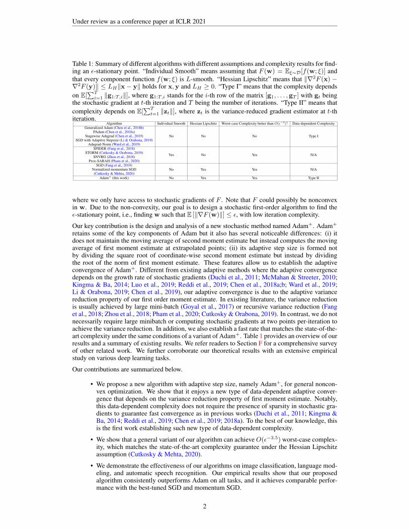
Table 1: Summary of different algorithms with different assumptions and complexity results for find-ing an ε-stationary point. “Individual Smooth” means assuming that F (w) = Eξ∼D[f(w; ξ)] andthat every component function f(w; ξ) is L-smooth. “Hessian Lipschitz” means that ‖∇2F (x) −∇2F (y)‖ ≤ LH‖x− y‖ holds for x,y and LH ≥ 0. “Type I” means that the complexity dependson E[

∑Ti=1 ‖g1:T,i‖], where g1:T,i stands for the i-th row of the matrix [g1, . . . ,gT ] with gt being

the stochastic gradient at t-th iteration and T being the number of iterations. “Type II” means thatcomplexity depends on E[

∑Tt=1 ‖zt‖], where zt is the variance-reduced gradient estimator at t-th

iteration.Algorithm Individual Smooth Hessian Lipschitz Worst-case Complexity better than O(ε−4)? Data-dependent Complexity

Generalized Adam (Chen et al., 2018b)PAdam (Chen et al., 2018a)

Stagewise Adagrad (Chen et al., 2019)SGD with Adaptive Stepsize (Li & Orabona, 2019)

Adagrad-Norm (Ward et al., 2019)

No No No Type I

SPIDER (Fang et al., 2018)STORM (Cutkosky & Orabona, 2019)

SNVRG (Zhou et al., 2018)Prox-SARAH (Pham et al., 2020)

Yes No Yes N/A

SGD (Fang et al., 2019)Normalized momentum SGD(Cutkosky & Mehta, 2020)

No Yes Yes N/A

Adam+ (this work) No Yes Yes Type II

where we only have access to stochastic gradients of F . Note that F could possibly be nonconvexin w. Due to the non-convexity, our goal is to design a stochastic first-order algorithm to find theε-stationary point, i.e., finding w such that E [‖∇F (w)‖] ≤ ε, with low iteration complexity.

Our key contribution is the design and analysis of a new stochastic method named Adam+. Adam+

retains some of the key components of Adam but it also has several noticeable differences: (i) itdoes not maintain the moving average of second moment estimate but instead computes the movingaverage of first moment estimate at extrapolated points; (ii) its adaptive step size is formed notby dividing the square root of coordinate-wise second moment estimate but instead by dividingthe root of the norm of first moment estimate. These features allow us to establish the adaptiveconvergence of Adam+. Different from existing adaptive methods where the adaptive convergencedepends on the growth rate of stochastic gradients (Duchi et al., 2011; McMahan & Streeter, 2010;Kingma & Ba, 2014; Luo et al., 2019; Reddi et al., 2019; Chen et al., 2018a;b; Ward et al., 2019;Li & Orabona, 2019; Chen et al., 2019), our adaptive convergence is due to the adaptive variancereduction property of our first order moment estimate. In existing literature, the variance reductionis usually achieved by large mini-batch (Goyal et al., 2017) or recursive variance reduction (Fanget al., 2018; Zhou et al., 2018; Pham et al., 2020; Cutkosky & Orabona, 2019). In contrast, we do notnecessarily require large minibatch or computing stochastic gradients at two points per-iteration toachieve the variance reduction. In addition, we also establish a fast rate that matches the state-of-the-art complexity under the same conditions of a variant of Adam+. Table 1 provides an overview of ourresults and a summary of existing results. We refer readers to Section F for a comprehensive surveyof other related work. We further corroborate our theoretical results with an extensive empiricalstudy on various deep learning tasks.

Our contributions are summarized below.

• We propose a new algorithm with adaptive step size, namely Adam+, for general noncon-vex optimization. We show that it enjoys a new type of data-dependent adaptive conver-gence that depends on the variance reduction property of first moment estimate. Notably,this data-dependent complexity does not require the presence of sparsity in stochastic gra-dients to guarantee fast convergence as in previous works (Duchi et al., 2011; Kingma &Ba, 2014; Reddi et al., 2019; Chen et al., 2019; 2018a). To the best of our knowledge, thisis the first work establishing such new type of data-dependent complexity.

• We show that a general variant of our algorithm can achieve O(ε−3.5) worst-case complex-ity, which matches the state-of-the-art complexity guarantee under the Hessian Lipschitzassumption (Cutkosky & Mehta, 2020).

• We demonstrate the effectiveness of our algorithms on image classification, language mod-eling, and automatic speech recognition. Our empirical results show that our proposedalgorithm consistently outperforms Adam on all tasks, and it achieves comparable perfor-mance with the best-tuned SGD and momentum SGD.

2


Algorithm 1 Adam+: Good default settings for the tested machine learning problems are α =0.1, a = 1, β = 0.1, ε0 = 10−8.

1: Require: α, a ≥ 1: stepsize parameters2: Require: β ∈ (0, 1): Exponential decay rates for the moment estimate3: Require: gt(w): unbiased stochastic gradient with parameters w at iteration t4: Require: w0: Initial parameter vector5: z0 = g0(w0)6: for t = 0, . . . , T do7: Set ηt = αβa

max(‖zt‖1/2,ε0)8: wt+1 = wt − ηtzt9: wt+1 = (1− 1/β)wt + 1/β ·wt+1

10: zt+1 = (1− β)zt + βgt+1(wt+1)11: end for

2 ALGORITHM AND THEORETICAL ANALYSISIn this section, we introduce our algorithm Adam+ (presented in Algorithm 1) and establish itsconvergence guarantees. Adam+ resembles Adam in several aspects but also has noticeable differ-ences. Similar to Adam, Adam+ also maintains an exponential moving average of first moment (i.e.,stochastic gradient), which is denoted by zt, and uses it for updating the solution in line 8. However,the difference is that the stochastic gradient is evaluated on an extrapolated data point wt+1, whichis an extrapolation of two previous updates wt and wt+1. Similar to Adam, Adam+ also uses anadaptive step size that is proportional to 1/‖zt‖1/2. Nonetheless, the difference lies at its adaptivestep size is directly computed from the square root of the norm of first moment estimate zt. Incontrast, Adam uses an adaptive step size that is proportional to 1/

√vt, where vt is an exponential

moving average of second moment estimate. These two key components of Adam+, i.e., extrap-olation and adaptive step size from the root norm of the first moment estimate, make it enjoy twonoticeable benefits: variance reduction of first moment estimate and adaptive convergence. We shallexplain these two benefits later.

Before moving to the theoretical analysis, we would like to make some remarks. First, it is worthmentioning that the moving average estimate with extrapolation is inspired by the literature ofstochastic compositional optimization (Wang et al., 2017). Wang et al. (2017) showed that the ex-trapolation helps balancing the noise in the gradients, reducing the bias in the estimates and givinga faster convergence rate. Here, our focus and analysis techniques are quite different. In fact, Wanget al. (2017) focuses on the compositional optimization while we consider a general nonconvex op-timization setting. Moreover, the analysis in (Wang et al., 2017) mainly deals with the error of thegradient estimator caused by the compositional nature of the problem, while our analysis focuseson carefully designing adaptive normalization to obtain an adaptive and fast convergence rates. Asimilar extrapolation scheme has been also employed in the algorithm NIGT by Cutkosky & Mehta(2020). In later sections, we will also provide a more general variant of Adam+ which subsumesNIGT as a special case.

Another important remark is that the update of Adam+ is very different from the famous Nesterov’smomentum method. In Nesterov’s momentum method, the update of wt+1 uses the stochastic gradi-ent at an extrapolated point wt+1 = wt+1 +γ(wt+1−wt) with a momentum parameter γ ∈ (0, 1).In contrast, in Adam+ the update of wt+1 is using the moving average estimate at an extrapolatedpoint wt+1 = wt+1 + (1/β − 1)(wt+1 −wt). Finally, Adam+ does not employ coordinate-wiselearning rates as in Adam, and hence it is expected to have better generalization performance ac-cording to Wilson et al. (2017).

2.1 ADAPTIVE VARIANCE REDUCTION AND ADAPTIVE CONVERGENCE

In this subsection, we analyze Adam+ by showing its variance reduction property and adaptiveconvergence. To this end, we make the following assumptions.

Assumption 1. There exists positive constants L,∆, LH , σ and an initial solution w0 such that

(i) F is L-smooth, i.e., ‖∇F (x)−∇F (y)‖ ≤ L ‖x− y‖ , ∀x,y ∈ Rd.

3


(ii) For ∀x ∈ Rd, we have access to a first-order stochastic oracle at time t gt(x) such thatE [gt(x)] = ∇F (x), E ‖gt(x)−∇F (x)‖2 ≤ σ2.

(iii) ∇F is a LH -smooth mapping, i.e., ‖∇2F (x)−∇2F (y)‖ ≤ LH‖x− y‖,∀x,y ∈ Rd.

(iv) F (w0)− F∗ ≤ ∆ <∞, where F∗ = infw∈Rd F (w).

Remark: Assumption 1 (i) and (ii), (iv) are standard assumptions made in literature of stochasticnon-convex optimization (Ghadimi & Lan, 2013). Assumption (iii) is the assumption that deviatesfrom typical analysis of stochastic methods. We leverage this assumption to explore the benefit ofmoving average, extrapolation and adaptive normalization. It is also used in some previous worksfor establishing fast rate of stochastic first-order methods for nonconvex optimization (Fang et al.,2019; Cutkosky & Mehta, 2020) and this assumption is essential to get fast rate due to the hardnessresult in (Arjevani et al., 2019). It is also the key assumption for finding a local minimum in previousworks (Carmon et al., 2018; Agarwal et al., 2017; Jin et al., 2017).

We might also assume that the stochastic gradient estimator in Algorithm 1 satisfies the followingvariance property.

Assumption 2. Assume that E[‖g0(w0) − ∇F (w0)‖2] ≤ σ20 and E[‖gt(wt) − ∇F (wt)‖2] ≤

σ2m, t ≥ 1.

Remark: When g0 (resp. gt) is implemented by a mini-batch stochastic gradient with mini-batchsize S, then σ2

0 (resp. σ2m) can be set as σ2/S by Assumption 1 (ii). We differentiate the initial

variance and intermediate variance because they contribute differently to the convergence.

We first introduce a lemma to characterize the variance of the moving average gradient estimator zt.

Lemma 1. Suppose Assumption 1 and Assumption 2 hold and a ≥ 1. Then, there exists a sequenceof random variables δt satisfying ‖zt −∇F (wt)‖ ≤ δt for ∀t ≥ 0,

E[δ2t+1

]≤(

1− β

2

)E[δ2t]

+ 2β2σ2m + E

[CL2

H‖wt+1 −wt‖4

β3

]≤(

1− β

2

)E[δ2t]

+ 2β2σ2m + E

[CL2

Hα4β4a−3‖zt‖2

],

where C = 1944.

Remark: Note that δt is an upper bound of ‖zt − ∇F (wt)‖, the above lemma can be used toillustrate the variance reduction effect for the gradient estimator zt. To this end, we can bound‖zt‖2 ≤ 2δ2t + 2‖∇F (wt)‖2, then the term CL2α4β4a−3δ2t can be canceled with −β/4δ2t withsmall enough α. Hence, we have Eδ2t+1 ≤ (1 − β/4)E[δ2t ] + 2β2σ2

m + cE[‖∇F (wt)‖2] with asmall constant c. As the algorithm converges with E[‖∇F (wt)‖2] and β decreases to zero, thevariance of zt will also decrease. Indeed, the above recursion of zt’s variance resembles that of therecursive variance reduced gradient estimators (e.g., SPIDER (Fang et al., 2018), STORM (Cutkosky& Orabona, 2019)). The benefit of using Adam+ is that we do not need to compute stochasticgradient twice at each iteration.

We can now state our convergence rates for Algorithm 1.

Theorem 1. Suppose Assumption 1 and Assumption 2 hold. Suppose ‖∇F (w)‖ ≤ G for anyw ∈ Rd. By choosing the parameters such that α4 ≤ 1

36CL2H

, α ≤ 14L , a = 1 and ε0 = βa, we have

1

T

T∑t=1

E ‖∇F (wt)‖2 ≤GE

[∑Tt=1 ‖zt‖

]T

+∆

αT+

18σ20

βT+ 30βσ2

m . (1)

In addition, suppose the initial batch size is T0 and the intermediate batch size is m, and chooseβ = T−b with 0 ≤ b ≤ 1, we have

1

T

T∑t=1

E ‖∇F (wt)‖2 ≤E[G∑Tt=1 ‖zt‖

]T

+∆

αT+

18σ2

T 1−bT0+

30σ2

mT b. (2)

4


Theorem 2. Suppose Assumption 1 and Assumption 2 hold. By choosing parameters such that640α3L

3/2H ≤ 1/120, a = 1, ε0 = 0, β = 1/T s with s = 2/3 then it takes T = O

(ε−4.5

)number

of iterations to ensure that

1

T

T∑t=1

E[‖∇F (wt)‖3/2

]≤ ε3/2, 1

TE[ T∑t=1

δ3/2t

]≤ ε3/2 .

Remarks:• From Theorem 1, we can observe that the convergence rate of Adam+ crucially depends on

the growth rate of E[∑T

t=1 ‖zt‖], which gives a data-dependent adaptive complexity. If

E[∑T

t=1 ‖zt‖]≤ Tα with α < 1, then the algorithm converges. Smaller α implies faster

convergence. Our goal is to ensure that 1T

∑Tt=1 E‖∇F (wt)‖2 ≤ ε2. Choosing b = 1−α,

m = O(1) and T0 = T 1−α = O(ε−2), and we end up with T = O(ε−

21−α

)complexity.

• Theorem 2 shows that in the ergodic sense, the Algorithm Adam+ always converges, andthe variance gets smaller when the number of iteration gets larger. Theorem 2 rules outthe case that the magnitude of zt converges to a constant and the bound (2) in Theorem 1becomes vacuous.

• To compare with Adam-style algorithms (e.g., Adam, AdaGrad), these algorithms’ con-vergence depend on the growth rate of stochastic gradient, i.e.,

∑di=1 ‖g1:T,i‖/T , where

g1:T,i = [g1,i, . . . , gT,i] denotes the i-th coordinate of all historical stochastic gradients.Hence, the data determines the growth rate of stochastic gradient. If the stochastic gradi-ents are not sparse, then its growth rate may not be slow and these Adam-style algorithmsmay suffer from slow convergence. In contrast, for Adam+ the convergence can be ac-celerated by the variance reduction property. Note that we have E

[∑Tt=1 ‖zt‖

]/T ≤

E[∑T

t=1(δt + ‖∇F (wt)‖)]/T . Hence, Adam+’s convergence depends on the variance

reduction property of zt.

2.2 A GENERAL VARIANT OF ADAM+: FAST CONVERGENCE WITH LARGE MINI-BATCH

Next, we introduce a more general variant of Adam+ by making a simple change. In particu-lar, we keep all steps the same as in Algorithm 1 except the adaptive step size is now set asηt = αβa

max(‖zt‖p,ε0) , where p ∈ [1/2, 1) is parameter. We refer to this general variant of Adam+

as power normalized Adam+ (Nadam+). This generalization allows us to compare with some ex-isting methods and to establish fast convergence rate. First, we notice that when setting p = 1 anda = 5/4 and β = 1/T 4/7, Nadam+ is almost the same as the stochastic method NIGT (Cutkosky& Mehta, 2020) with only some minor differences. However, we observed that normalizing by ‖zt‖leads to slow convergence in practice, so we are instead interested in p < 1. Below, we will showthat NAdam+ with p < 1 can achieve a fast rate of 1/ε3.5, which is the same as NIGT.Theorem 3. Under the same assumption as in Theorem 1, further assume σ2

0 = σ2/T0 and σ2m =

σ2/m. By using the step size ηt = αβ4/3

max(‖zt‖2/3,ε0)in Algorithm 1 with CL2α4 ≤ 1/14, ε0 = 2β4/3,

in order to have E [‖∇F (wτ )‖] ≤ ε for a randomly selected solution wτ from {w1, . . . ,wT }, it suf-fice to set β = O(ε1/2), T = O(ε−2), the initial batch size T0 = 1/β = O(ε−1/2), the intermediatebatch size as m = 1/β3 = O(ε−3/2), which ends up with the total complexity O(ε−3.5).

Remark: Note that the above theorem establishes the fast convergence rate for Nadam+ with p =2/3. Indeed, we can also establish a fast rate of Adam+ (where p = 1/2) in the order ofO(1/ε3.625)with details provided in the Appendix E.

3 EXPERIMENTS

In this section, we conduct empirical studies to verify the effectiveness of the proposed algorithmon three different tasks: image classification on CIFAR10 and CIFAR100 dataset (Krizhevsky et al.,

5


0 100 200 300 400

Number of Epochs

0.9

0.92

0.94

0.96

0.98

1

Tra

inin

g A

ccu

racy

ResNet18 training on CIFAR10

SGD

Momentum SGD

Adagrad

Adam

NIGT

Adam+

0 100 200 300 400

Number of Epochs

0.75

0.8

0.85

0.9

0.95

Test

Accu

racy


SGD

Momentum SGD

Adagrad

Adam

NIGT

Adam+

Figure 1: Comparison of optimization methods for ResNet18 Training on CIFAR10.

2009), language modeling on Wiki-Text2 dataset (Merity, 2016) and automatic speech recognitionon SWB-300 dataset (Saon et al., 2017). We choose tasks from different domains to demonstratethe applicability for the real-world deep learning tasks in a broad sense. The detailed descriptionis presented in Table 2. We compare our algorithm Adam+ with SGD, momentum SGD, Adagrad,NIGT and Adam. We choose the same random initialization for each algorithm, and run a fixednumber of epochs for every task. For Adam we choose the default setting β1 = 0.9 and β2 = 0.999as in the original Adam paper.

Table 2: Summary of setups in the experiments.Domain Task Architecture Dataset

Computer Vision Image Classification ResNet18 CIFAR10Computer Vision Image Classification VGG19 CIFAR100

Natural Language Processing Language Modeling Two-layer LSTM Wiki-Text2Automatic Speech Recognition Speech Recognition Six-layer BiLSTM SWB-300

3.1 IMAGE CLASSIFICATION

CIFAR10 and CIFAR100 In the first experiment, we consider training ResNet18 (He et al., 2016)and VGG19 (Simonyan & Zisserman, 2014) to do image classification task on CIFAR10 and CI-FAR100 dataset respectively. For every optimizer, we use batch size 128 and run 350 epochs. ForSGD and momentum SGD, we set the initial learning rate to be 0.1 for the first 150 epochs, and thelearning rate is decreased by a factor of 10 for every 100 epochs. For Adagrad and Adam, the initiallearning rate is tuned from {0.1, 0.01, 0.001} and we choose the one with the best performance. Thebest initial learning rates for Adagrad and Adam are 0.01 and 0.001 respectively. For NIGT, wetune the their momentum parameter from {0.01, 0.1, 0.9} (the best momentum parameter we foundis 0.9) and the learning rate is chosen the same as in SGD. For Adam+, the learning rate is set ac-cording to Algorithm 1, in which we choose β = 0.1 and the value of α is the same as the learningrate used in SGD. We report training and test accuracy versus the number of epochs in Figure 1 forCIFAR10 and Figure 2 for CIFAR100. We observe that our algorithm consistently outperforms allother algorithms on both CIFAR10 and CIFAR100, in terms of both training and testing accuracy.Notably, we have some interesting observations for the training of VGG19 on CIFAR100. First, bothAdam+ and NIGT significantly outperform SGD, momentum SGD, Adagrad and Adam. Second,Adam+ achieves almost the same final accuracy as NIGT, and Adam+ converges much faster in theearly stage of the training.

3.2 LANGUAGE MODELING

Wiki-text2 In the second experiment, we consider the language modeling task on WikiText-2dataset. We use a 2-layer LSTM (Hochreiter & Schmidhuber, 1997). The size of word embeddingsis 650 and the number of hidden units per layer is 650. We run every algorithm for 40 epochs, withbatch size 20 and dropout ratio 0.5. For SGD and momentum SGD, we tune the initial learning ratefrom {0.1, 0.2, 0.5, 5, 10, 20} and decrease the learning rate by factor of 4 when the validation error

6


0 100 200 300 400

Number of Epochs

0.85

0.9

0.95

1

Tra

inin

g A

ccu

racy

VGG19 training on CIFAR100

SGD

Momentum SGD

Adagrad

Adam

NIGT

Adam+

0 100 200 300 400

Number of Epochs

0.3

0.4

0.5

0.6

0.7

Test

Accu

racy

VGG19 training on CIFAR100

SGD

Momentum SGD

Adagrad

Adam

NIGT

Adam+

Figure 2: Comparison of optimization methods for VGG19 training on CIFAR100.

0 10 20 30 40

Number of Epochs

0

50

100

150

200

Tra

inin

g P

erp

lexit

y

LSTM Training on Wikitext-2

SGD

Momentum SGD

Adagrad

Adam

NIGT

Adam+

0 10 20 30 40

Number of Epochs

50

100

150

200

250

300

350

Test

Perp

lexit

y

LSTM Training on Wikitext-2

SGD

Momentum SGD

Adagrad

Adam

NIGT

Adam+

Figure 3: Comparison of optimization methods for two-layers LSTM training on WikiText-2.

saturates. For Adagrad and Adam, we tune the initial learning rate from {0.001, 0.01, 0.1, 1.0}. Wereport the best performance for these methods across the range of learning rate. The best initiallearning rates for Adagrad and Adam are 0.01 and 0.001 respectively. For NIGT, we tune theinitial value of learning rate from the same range as in SGD, and tune the momentum parameter βfrom {0.01, 0.1, 0.9}, and the best parameter choice is β = 0.9. The learning rate and β are bothdecreased by a factor of 4 when the validation error saturates. For Adam+, we follow the sametuning strategy as NIGT.

We report both training and test perplexity versus the number of epochs in Figure 3. From the Fig-ure, we have the following observations: First, in terms of training perplexity, our algorithm achievescomparable performance with SGD and momentum SGD and outperforms Adagrad and NIGT, andit is worse than Adam. Second, in terms of test perplexity, our algorithm outperforms Adam, Ada-grad, NIGT and momentum SGD, and it is comparable to SGD. An interesting observation is thatAdam does not generalize well even if it has fast convergence in terms of training error, which isconsistent with the observations in (Wilson et al., 2017).

3.3 AUTOMATIC SPEECH RECOGNITION

SWB-300 In the third experiment, we consider the automatic speech recognition task on SWB-300dataset (Saon et al., 2017). SWB-300 contains roughly 300 hours of training data of over 4 millionsamples (30GB) and roughly 6 hours of held-out data of over 0.08 million samples (0.6GB). Eachtraining sample is a fusion of FMLLR (40-dim), i-Vector (100-dim), and logmel with its delta anddouble delta. The acoustic model is a long short-term memory (LSTM) model with 6 bi-directionallayers. Each layer contains 1,024 cells (512 cells in each direction). On top of the LSTM layers,there is a linear projection layer with 256 hidden units, followed by a softmax output layer with32,000 (i.e., 32,000 classes) units corresponding to context-dependent HMM states. The LSTMis unrolled with 21 frames and trained with non-overlapping feature sub-sequences of that length.This model contains over 43 million parameters and is about 165MB large. The training takesabout 20 hours on 1 V100 GPU. To compare, we adopt the well-tuned Momentum SGD strategyas described in (Zhang et al., 2019) for this task as the baseline: batch size is 256, learning rate is

7


0 5 10 15 20

Number of Epochs

1

1.5

2

2.5

3

3.5

4

Tra

inin

g L

oss

LSTM Training on SWB-300

SGD

Momentum SGD

Adagrad

Adam

NIGT

Adam+

0 5 10 15 20

Number of Epochs

1

1.5

2

2.5

3

3.5

4

Test

Lo

ss

LSTM Training on SWB-300

SGD

Momentum SGD

Adagrad

Adam

NIGT

Adam+

Figure 4: Comparison of optimization methods for six-layers LSTM training on SWB-300.

0 2 4 6 8 10 12 14

104

0

2

4

6

8

1010

4 ResNet18 training on CIFAR10

Adam+

0 5 10 15

104

0

2

4

6

8

10

1210

4VGG19 training on CIFAR100

Adam+

Figure 5: The growth of quantity∑ti=1 ‖zi‖ in Adam+

0.1 for the first 10 epochs and then annealed by√

0.5 for another 10 epochs, with momentum 0.9.We grid search the learning rate of Adam and Adagrad from {0.1, 0.01, 0.001}, and report the bestconfiguration we have found (Adam with learning rate 0.001 and Adagrad with learning rate 0.01).For NIGT, we also follow the same learning rate setup (including annealing) as in Momentum SGDbaseline. In addition, we fine tuned β in NIGT by exploring β in {0.01, 0.1, 0.9} and reported thebest configuration (β=0.9). For Adam+, we follow the same learning rate and annealing strategy asin the Momentum SGD and tuned β in the same way as in NGIT, reporting the best configuration(β=0.01). From Figure 4, Adam+ achieves the indistinguishable training loss and held-out loss w.r.t.well-tuned Momentum SGD baseline and significantly outperforms the other optimizers.

3.4 GROWTH RATE OF∑ti=1 ‖zi‖

In this subsection, we consider the growth rate of∑ti=1 ‖zi‖, since they crucially affect the conver-

gence rate as shown in Theorem 1. We report the results of both ResNet18 training on CIFAR10dataset and VGG19 training on CIFAR100 dataset. From Figure 5, we can observe that it quicklyreaches a plateau and then grows at a very slow rate with respect to the number of iterations. Thisphenomenon verifies the variance reduction effect and also explains the reason why Adam+ enjoysa fast convergence speed in practice.

4 CONCLUSIONIn this paper, we design a new algorithm named Adam+ to train deep neural networks efficiently.Different from Adam, Adam+ updates the solution using moving average of stochastic gradientscalculated at the extrapolated points and adaptive normalization on only first-order statistics ofstochastic gradients. We establish data-dependent adaptive complexity results for Adam+ fromthe perspective of adaptive variance reduction, and also show that a variant of Adam+ achievesstate-of-the-art complexity. Extensive empirical studies on several tasks verify the effectiveness ofthe proposed algorithm. We also empirically show that the slow growth rate of the new gradientestimator, providing the reason why Adam+ enjoys fast convergence in practice.

8


REFERENCES

Naman Agarwal, Zeyuan Allen-Zhu, Brian Bullins, Elad Hazan, and Tengyu Ma. Finding approxi-mate local minima faster than gradient descent. In Proceedings of the 49th Annual ACM SIGACTSymposium on Theory of Computing, pp. 1195–1199, 2017.

Zeyuan Allen-Zhu and Elad Hazan. Variance reduction for faster non-convex optimization. InInternational conference on machine learning, pp. 699–707, 2016.

Yossi Arjevani, Yair Carmon, John C Duchi, Dylan J Foster, Nathan Srebro, and Blake Woodworth.Lower bounds for non-convex stochastic optimization. arXiv preprint arXiv:1912.02365, 2019.

Yair Carmon, John C Duchi, Oliver Hinder, and Aaron Sidford. Accelerated methods for nonconvexoptimization. SIAM Journal on Optimization, 28(2):1751–1772, 2018.

Jinghui Chen, Dongruo Zhou, Yiqi Tang, Ziyan Yang, and Quanquan Gu. Closing the gener-alization gap of adaptive gradient methods in training deep neural networks. arXiv preprintarXiv:1806.06763, 2018a.

Xiangyi Chen, Sijia Liu, Ruoyu Sun, and Mingyi Hong. On the convergence of a class of Adam-typealgorithms for non-convex optimization. arXiv preprint arXiv:1808.02941, 2018b.

Zaiyi Chen, Zhuoning Yuan, Jinfeng Yi, Bowen Zhou, Enhong Chen, and Tianbao Yang. Universalstagewise learning for non-convex problems with convergence on averaged solutions. In Interna-tional Conference on Learning Representations, 2019.

Ashok Cutkosky and Harsh Mehta. Momentum improves normalized SGD. arXiv preprintarXiv:2002.03305, 2020.

Ashok Cutkosky and Francesco Orabona. Momentum-based variance reduction in non-convex SGD.In Advances in Neural Information Processing Systems, pp. 15236–15245, 2019.

John Duchi, Elad Hazan, and Yoram Singer. Adaptive subgradient methods for online learning andstochastic optimization. Journal of Machine Learning Research, 12(Jul):2121–2159, 2011.

Cong Fang, Chris Junchi Li, Zhouchen Lin, and Tong Zhang. Spider: Near-optimal non-convex op-timization via stochastic path-integrated differential estimator. In Advances in Neural InformationProcessing Systems, pp. 689–699, 2018.

Cong Fang, Zhouchen Lin, and Tong Zhang. Sharp analysis for nonconvex SGD escaping fromsaddle points. arXiv preprint arXiv:1902.00247, 2019.

Saeed Ghadimi and Guanghui Lan. Stochastic first-and zeroth-order methods for nonconvex stochas-tic programming. SIAM Journal on Optimization, 23(4):2341–2368, 2013.

Priya Goyal, Piotr Dollár, Ross Girshick, Pieter Noordhuis, Lukasz Wesolowski, Aapo Kyrola, An-drew Tulloch, Yangqing Jia, and Kaiming He. Accurate, large minibatch SGD: Training imagenetin 1 hour. arXiv preprint arXiv:1706.02677, 2017.

Kaiming He, Xiangyu Zhang, Shaoqing Ren, and Jian Sun. Deep residual learning for image recog-nition. In Proceedings of the IEEE conference on computer vision and pattern recognition, pp.770–778, 2016.

Sepp Hochreiter and Jürgen Schmidhuber. Long short-term memory. Neural computation, 9(8):1735–1780, 1997.

Chi Jin, Rong Ge, Praneeth Netrapalli, Sham M Kakade, and Michael I Jordan. How to escapesaddle points efficiently. arXiv preprint arXiv:1703.00887, 2017.

Rie Johnson and Tong Zhang. Accelerating stochastic gradient descent using predictive variancereduction. In Advances in neural information processing systems, pp. 315–323, 2013.

Diederik P Kingma and Jimmy Ba. Adam: A method for stochastic optimization. arXiv preprintarXiv:1412.6980, 2014.

9


Alex Krizhevsky, Vinod Nair, and Geoffrey Hinton. CIFAR-10 and CIFAR-100 datasets. URl:https://www. cs. toronto. edu/kriz/cifar. html, 6:1, 2009.

Lihua Lei, Cheng Ju, Jianbo Chen, and Michael I Jordan. Non-convex finite-sum optimization viaSCSG methods. In Advances in Neural Information Processing Systems, pp. 2348–2358, 2017.

Kfir Levy. Online to offline conversions, universality and adaptive minibatch sizes. In Advances inNeural Information Processing Systems, pp. 1613–1622, 2017.

Xiaoyu Li and Francesco Orabona. On the convergence of stochastic gradient descent with adaptivestepsizes. In The 22nd International Conference on Artificial Intelligence and Statistics, pp. 983–992, 2019.

Liyuan Liu, Haoming Jiang, Pengcheng He, Weizhu Chen, Xiaodong Liu, Jianfeng Gao, and JiaweiHan. On the variance of the adaptive learning rate and beyond. arXiv preprint arXiv:1908.03265,2019.

Liangchen Luo, Yuanhao Xiong, Yan Liu, and Xu Sun. Adaptive gradient methods with dynamicbound of learning rate. arXiv preprint arXiv:1902.09843, 2019.

H Brendan McMahan and Matthew Streeter. Adaptive bound optimization for online convex opti-mization. arXiv preprint arXiv:1002.4908, 2010.

Stephen Merity. The WikiText long term dependency language modeling dataset. Salesforce Meta-mind, 9, 2016.

Nhan H Pham, Lam M Nguyen, Dzung T Phan, and Quoc Tran-Dinh. ProxSARAH: An efficientalgorithmic framework for stochastic composite nonconvex optimization. Journal of MachineLearning Research, 21(110):1–48, 2020.

Sashank J Reddi, Ahmed Hefny, Suvrit Sra, Barnabas Poczos, and Alex Smola. Stochastic variancereduction for nonconvex optimization. In International conference on machine learning, pp. 314–323, 2016.

Sashank J Reddi, Satyen Kale, and Sanjiv Kumar. On the convergence of Adam and beyond. arXivpreprint arXiv:1904.09237, 2019.

George Saon, Gakuto Kurata, Tom Sercu, Kartik Audhkhasi, Samuel Thomas, Dimitrios Dimitri-adis, Xiaodong Cui, Bhuvana Ramabhadran, Michael Picheny, Lynn-Li Lim, Bergul Roomi, andPhil Hall. English conversational telephone speech recognition by humans and machines. InInterspeech, 2017.

Karen Simonyan and Andrew Zisserman. Very deep convolutional networks for large-scale imagerecognition. arXiv preprint arXiv:1409.1556, 2014.

Tijmen Tieleman and Geoffrey Hinton. Lecture 6.5-rmsprop, coursera: Neural networks for machinelearning. University of Toronto, Technical Report, 2012.

Mengdi Wang, Ethan X Fang, and Han Liu. Stochastic compositional gradient descent: algorithmsfor minimizing compositions of expected-value functions. Mathematical Programming, 161(1-2):419–449, 2017.

Zhe Wang, Kaiyi Ji, Yi Zhou, Yingbin Liang, and Vahid Tarokh. SpiderBoost and momentum:Faster variance reduction algorithms. In Advances in Neural Information Processing Systems, pp.2406–2416, 2019.

Rachel Ward, Xiaoxia Wu, and Leon Bottou. AdaGrad stepsizes: Sharp convergence over noncon-vex landscapes. In International Conference on Machine Learning, pp. 6677–6686, 2019.

Ashia C Wilson, Rebecca Roelofs, Mitchell Stern, Nati Srebro, and Benjamin Recht. The marginalvalue of adaptive gradient methods in machine learning. In Advances in Neural InformationProcessing Systems, pp. 4148–4158, 2017.

Yang You, Igor Gitman, and Boris Ginsburg. Scaling SGD batch size to 32k for imagenet training.arXiv preprint arXiv:1708.03888, 6, 2017.

10


Yang You, Jing Li, Sashank Reddi, Jonathan Hseu, Sanjiv Kumar, Srinadh Bhojanapalli, XiaodanSong, James Demmel, Kurt Keutzer, and Cho-Jui Hsieh. Large batch optimization for deeplearning: Training BERT in 76 minutes. arXiv preprint arXiv:1904.00962, 2019.

Jingzhao Zhang, Hongzhou Lin, Suvrit Sra, and Ali Jadbabaie. On complexity of finding stationarypoints of nonsmooth nonconvex functions. arXiv preprint arXiv:2002.04130, 2020.

Wei Zhang, Xiaodong Cui, Ulrich Finkler, Brian Kingsbury, George Saon, David Kung, and MichaelPicheny. Distributed deep learning strategies for automatic speech recognition. In ICASSP’2019,May 2019.

Dongruo Zhou, Pan Xu, and Quanquan Gu. Stochastic nested variance reduction for nonconvexoptimization. In Advances in Neural Information Processing Systems, pp. 3921–3932, 2018.

11


A PROOF OF LEMMA 1

Proof. The proof is similar to that of Lemma 12 in (Wang et al., 2017). Define

ζ(t)k =

{β(1− β)t−k if t ≥ k > 0

(1− β)t−k if t ≥ k = 0(3)

By the definition of ζ(k)t and the update of Algorithm 1, we have

ζ(t+1)k = (1− β)ζ

(t)k ,

t∑k=0

ζ(t)k = 1, wt =

t∑k=0

ζ(t)k wt+1, zt+1 =

t∑k=0

ζ(t)k ∇f(wt+1; ξt+1).

Define mt+1 =∑tk=0 ζ

(t)k ‖wt+1 − wk+1‖2, nt+1 =

∑tk=0 ζ

(t)k [∇f(wk+1; ξk+1)− F (wk+1)],

where∇f(wk+1; ξk+1) is an unbiased stochastic first-order oracle for F (wk+1) with bounded vari-ance σ2

m. Note that∇F is a LH -smooth mapping (according to Assumption 1 (iii)), then by Lemma10 of (Wang et al., 2017), we have

‖zt −∇F (wt)‖2 ≤ (LHmt + ‖nt‖)2 ≤ 2L2Hm

2t + 2‖nt‖2.

Define qt+1 =∑tk=0 ζ

(t)k ‖wt+1 − wk+1‖. According to Lemma 11 (a) and (b) of (Wang et al.,

2017), we have

mt+1 + 4q2t+1 ≤(

1− β

2

)(mt + 4q2t

)+

18

β‖wt+1 −wt‖2.

Taking squares on both sides of the inequality and using the fact that (a+b)2 ≤ (1+ β2 )a2+(1+ 2

β )b2

for β > 0, we have(mt+1 + 4q2t+1

)2 ≤ (1 +β

2

)(1− β

2

)2 (mt + 4q2t

)2+

(1 +

2

β

)324

β2‖wt+1 −wt‖4

≤(

1− β

2

)(mt + 4q2t )2 +

972

β3‖wt+1 −wt‖4 ,

(4)

where the last inequality holds since 1/β ≥ 1.

Define δ2t = 2L2H(mt + 4q2t )2 + 2 ‖nt‖2, then we have ‖zt −∇F (wt)‖2 ≤ δ2t for all t. Denote

Ft+1 by the σ-algebra generated by ξ1, . . . , ξt+1. Taking the summation of (4) and according to thebound of nt derived in Lemma 11 (c) of (Wang et al., 2017), we have

E[δ2t+1|Ft+1

]≤(

1− β

2

)δ2t + 2β2σ2

m +1944L2

H ‖wt+1 −wt‖4

β3,

Taking expectation on both sides yields

E[δ2t+1

]≤(

1− β

2

)E[δ2t]

+ 2β2σ2m + E

[1944L2

H‖wt+1 −wt‖4

β3

].

Note that ηt = αβa

max(‖zt‖1/2,ε0), we have

E[δ2t+1

]≤(

1− β

2

)E[δ2t]

+ 2β2σ2m + E

[CL2α4β4a−3‖zt‖2

].

B PROOF OF THEOREM 1

Proof. By Lemma 1 and the update rule of Algorithm 1, we have

E[δ2t+1

]≤(

1− β

2

)E[δ2t]

+ 2β2σ2m + E

[CL2

Hα4β4a‖zt‖4

β3(max(‖zt‖1/2, ε0))4

]≤(

1− β

2

)E[δ2t]

+ 2β2σ2m + E

[2CL2

Hα4β4(‖δt‖2 + ‖∇F (wt)‖2)

β3

],

(5)

12


where the second inequality holds since (max(‖zt‖1/2, ε0))4 ≥ ‖zt‖2 and ‖zt‖2 ≤ 2‖δt‖2 +

2 ‖∇F (wt)‖2.

Note that 2CL2Hα

4 ≤ 1/18. Plugging it in (5), we have

8β

18E[δ2t]≤ E

[δ2t − δ2t+1

]+ 2β2σ2

m + E[β

18‖∇F (wt)‖2

]. (6)

Summing over t = 1, . . . , T on both sides of (6) and with some simple algebra, we haveT∑t=1

E[δ2t]≤

T∑t=1

E

[3(δ2t − δ2t+1

)β

]+

T∑t=1

5βσ2m +

T∑t=1

E[

1

8‖∇F (wt)‖2

]. (7)

By Assumption 1 (i) and by the property of L-smooth function, we know that

F (wt+1) ≤ F (wt) +∇>F (wt)(wt+1 −wt) +L

2‖wt+1 −wt‖2

=F (wt)− ηt∇>F (wt)zt +η2tL

2‖zt‖2

≤ F (wt)− ηt∇>F (wt)(zt −∇F (wt) +∇F (wt)) + η2tL(‖zt −∇F (wt)‖2 + ‖∇F (wt)‖2

)= F (wt)− (ηt − η2tL)‖∇F (wt)‖2 − ηt∇>F (wt)(zt −∇F (wt)) + η2tL ‖zt − F (wt)‖2

≤ F (wt)−(ηt

2− η2tL

)‖∇F (wt)‖2 +

(ηt2

+ η2tL)‖zt − F (wt)‖2 .

Noting that ηt = αβa

max(‖zt‖1/2,ε0), α ≤ 1/4L and ε0 = βa, we know that ηtL ≤ 1/4. Hence we

have

‖∇F (wt)‖2 ≤4(F (wt)− F (wt+1))

ηt+ 3‖zt −∇F (wt)‖2.

Taking summation over t = 1, . . . , T and taking expectation yieldT∑t=1

E ‖∇F (wt)‖2 ≤ E

[T∑t=1

4(F (wt)− F (wt+1))

ηt

]+ 3

T∑t=1

E‖zt −∇F (wt)‖2

≤ E

[T∑t=1

4(F (wt)− F (wt+1))

ηt

]+ 3

T∑t=1

E[δ2t].

(8)

Combining (7) and (8) yieldsT∑t=1

E ‖∇F (wt)‖2 ≤ E

[T∑t=1

4(F (wt)− F (wt+1))

ηt

]+

T∑t=1

E

[9(δ2t − δ2t+1

)β

]

+

T∑t=1

15βσ2m +

T∑t=1

E[

3

8‖∇F (wt)‖2

].

By some simple algebra, we haveT∑t=1

E ‖∇F (wt)‖2 ≤ E

[T∑t=1

8(F (wt)− F (wt+1))

ηt

]+

T∑t=1

E

[18(δ2t − δ2t+1

)β

]+

T∑t=1

30βσ2m.

Then we have

1

T

T∑t=1

E ‖∇F (wt)‖2 ≤ E

[T∑t=1

8 max(‖zt‖1/2, ε0

)(F (wt)− F (wt+1))

αβaT

]+

18σ20

βT+30βσ2

m. (9)

Noting that |F (wt)− F (wt+1)| ≤ Gηt‖zt‖, we have

1

T

T∑t=1

E ‖∇F (wt)‖2 ≤8GE

[∑Tt=1 ‖zt‖

]T

+∆

αT+

18σ20

βT+ 30βσ2

m. (10)

13


C PROOF OF THEOREM 2

Before introducing the proof, we first introduce several lemmas which are useful for our analysis.

Lemma 2. Adam+ with ηt = αβ

max(‖zt‖1/2,ε0)and ε0 = 0 satisfies

F (wt+1)− F (wt) ≤ αβ(−‖∇F (wt)‖3/2

6+ 9‖zt −∇F (wt)‖3/2

)+

64α4β4L3

3.

Proof. By the L-smoothness and the update of the algorithm, we have

F (wt+1)− F (wt) ≤ ∇>F (wt)(wt+1 −wt) +L‖wt+1 −wt‖2

2

≤ −αβ · 〈∇F (wt), zt〉max

(‖zt‖1/2, ε0

) +α2β2L‖zt‖2(

max(‖zt‖1/2, ε0

))2 . (11)

Define ∆t = zt −∇F (wt). If ‖∇F (wt)‖ ≥ 2‖∆t‖, we have

− 〈zt,∇F (wt)〉max

(‖zt‖1/2, ε0

) = − ‖∇F (wt)‖2 + 〈∆t,∇F (wt)〉max

(‖∇F (wt) + ∆t‖1/2, ε0

)≤ − ‖∇F (wt)‖2

2‖∇F (wt) + ∆t‖1/2≤ −‖∇F (wt)‖3/2

3

≤ −‖∇F (wt)‖3/2

3+ 8‖∆t‖3/2.

(12)

If ‖∇F (wt)‖ ≤ 2‖∆t‖, we have


(‖zt‖1/2, ε0

) = − ‖∇F (wt)‖2 + 〈∆t,∇F (wt)〉max

(‖∇F (wt) + ∆t‖1/2, ε0

)≤ 6‖∆t‖2

‖∆t‖1/2= 6‖∆t‖3/2 ≤ −

‖∇F (wt)‖3/2

3+ 8‖∆t‖3/2.

(13)

By (12) and (13), we have


(‖zt‖1/2, ε0

) ≤ −‖∇F (wt)‖3/2

3+ 8‖∆t‖3/2. (14)

By (11) and (14), we have

F (wt+1)− F (wt) ≤ αβ(‖∇F (wt)‖3/2

3+ 8‖∆t‖3/2

)+ α2β2L‖zt‖

= αβ

(−‖∇F (wt)‖3/2

3+ 8‖∆t‖3/2

)+ α2β2Lmin

x>0

(2‖zt‖3/2

3x+x2

3

)≤ αβ

(−‖∇F (wt)‖3/2

3+ 8‖∆t‖3/2

)+ α2β2L

(2‖zt‖3/2

3(8αβL)+

64α2β2L2

3

)≤ αβ

(−‖∇F (wt)‖3/2

6+ 9‖∆t‖3/2

)+

64α4β4L3

3,

where the last inequality holds because ‖zt‖3/2 ≤ 2‖∇F (wt)‖3/2 + 2‖∆t‖3/2.

Lemma 3. For Adam+ with ηt = αβ

max(‖zt‖1/2,ε0), there exist random variables δt such that

E[δ3/2t+1

]≤(

1− β

2

)E[δ3/2t

]+ 2β3/2σ3/2 + E

[320L

3/2H ‖wt+1 −wt‖3

β2

].

14


Proof. The proof shares the similar spirit of Lemma 12 in (Wang et al., 2017), but we adapt theproof for our purpose. Define

ζ(t)k =

{β(1− β)t−k if t ≥ k > 0

(1− β)t−k if t ≥ k = 0(15)

By the definition of ζ(k)t and the update of Algorithm 1, we have

ζ(t+1)k = (1− β)ζ

(t)k ,

t∑k=0

ζ(t)k = 1, wt =

t∑k=0

ζ(t)k wt+1, zt+1 =

t∑k=0

ζ(t)k ∇f(wt+1; ξt+1).

Define mt+1 =∑tk=0 ζ

(t)k ‖wt+1 − wk+1‖2, nt+1 =

∑tk=0 ζ

(t)k [∇f(wk+1; ξk+1)− F (wk+1)],

where∇f(wk+1; ξk+1) is an unbiased stochastic first-order oracle for F (wk+1) with bounded vari-ance σ2. Note that ∇F is a LH -smooth mapping (according to Assumption 1), then by Lemma 10of (Wang et al., 2017), we have

‖zt −∇F (wt)‖3/2 ≤ (LHmt + ‖nt‖)3/2 ≤ 2L3/2H m

3/2t + 2‖nt‖3/2.

Define qt+1 =∑tk=0 ζ

(t)k ‖wt+1 − wk+1‖. According to Lemma 11 (a) and (b) of (Wang et al.,

2017), we have

mt+1 + 4q2t+1 ≤(

1− β

2

)(mt + 4q2t

)+

18

β‖wt+1 −wt‖2.

Taking the power 3/2 on both sides of the inequality and using the fact that (a + b)3/2 ≤√1 + β

2 a3/2 +

√1 + 2

β b3/2 for β > 0, we have(

mt+1 + 4q2t+1

)3/2≤(

1 +β

2

)1/2(1− β

2

)3/2 (mt + 4q2t

)3/2+

(1 +

2

β

)1/280

β3/2‖wt+1 −wt‖3

≤(

1− β

2

)(mt + 4q2t )3/2 +

160

β2‖wt+1 −wt‖3 ,

(16)

where the last inequality holds since 1/β ≥ 1.

By the definition of nt, we have nt+1 = (1 − β)nt + β(∇f(wt+1) − F (wt+1)). Denote Ft+1 bythe σ-algebra generated by ξ1, . . . , ξt+1. Noting that

E[‖nt+1‖3/2|Ft+1

]≤(E[‖nt+1‖2|Ft+1

])3/4 ≤ (1− β/2)3/2‖nt‖3/2 + β3/2σ3/2, (17)

where the last inequality holds by invoking Lemma 11(c) of (Wang et al., 2017). Define δ3/2t =

2L3/2H (mt + 4q2t )3/2 + 2‖nt‖3/2, then we have ‖zt −∇F (wt)‖3/2 ≤ δ

3/2t for all t. According

to (16) and (17), we have

E[δ3/2t+1|Ft+1

]≤(

1− β

2

)‖δt‖3/2 + 2β3/2σ3/2 +

320L3/2H ‖wt+1 −wt‖3

β2.

Taking expectation on both sides yields

E[δ3/2t+1

]≤(

1− β

2

)E[δ3/2t

]+ 2β3/2σ3/2 + E

[320L

3/2H ‖wt+1 −wt‖3

β2

].

Lemma 4. Adam+ with learning rate ηt = αβ

max(‖zt‖1/2,ε0)and 640α3L

3/2H ≤ 1/120 satisfies

1

T

T∑t=1

E[‖∇F (wt)‖3/2

]≤ 101∆

αβT+

2727E[δ3/21

]βT

+ 4545β1/2σ3/2 +3β3L3/2

100.

To ensure that 1T

∑Tt=1 E

[‖∇F (wt)‖3/2

]≤ ε3/2, we can choose β = ε3, T = O(ε−9/2).

15


Proof. By Lemma 3 and noting that ηt = αβ

max(‖zt‖1/2,ε0), we have

E[δ3/2t+1

]≤(

1− β

2

)E[δ3/2t

]+ 2β3/2σ3/2 + E

[320L

3/2H α3β3‖zt‖3/2

β2

]

≤(

1− β

2

)E[δ3/2t

]+ 2β3/2σ3/2 + E

[640L

3/2H α3β

(‖∇F (wt)‖3/2 + ‖δt‖3/2

)].

(18)

Note that 640α3L3/2H ≤ 1/120. Plugging it into (18), we have

59β

120E[δ3/2t

]≤ E

[δ3/2t − δ3/2t+1

]+ 2β3/2σ3/2 + E

[β

120‖∇F (wt)‖3/2

]. (19)

Summing over t = 1, . . . , T on both sides of (19) and with some simple algebra, we haveT∑t=1

E[δ3/2t

]≤

T∑t=1

E

[3(δ

3/2t − δ3/2t+1)

β

]+

T∑t=1

5β1/2σ3/2 +

T∑t=1

E[

1

59‖∇F (wt)‖2/3

].

By Lemma 2, taking expectation on both sides, we have

E [F (wt+1)− F (wt)] ≤ αβ

(−E[‖∇F (wt)‖3/2

]6

+ 9E[δ3/2t

])+

64α4β4L3

3. (20)

Summing (20) over t = 1, . . . , T yields

5

504αβ

T∑t=1

E[‖∇F (wt)‖3/2

]≤ F (w1)−F∗+αβ

27E[δ3/21

]β

+

T∑t=1

45β1/2σ3/2

+64α4β4L3T

3.

Hence, we have

1

T

T∑t=1

E[‖∇F (wt)‖3/2

]≤ 101∆

αβT+

2727E[δ3/21

]β

+ 4545β1/2σ3/2 + 2155α3β3L3

≤ 101∆

αβT+

2727E[δ3/21

]βT

+ 4545β1/2σ3/2 +3β3L3/2

100.

Lemma 5. Under the same setting of Lemma 4, we know that to ensure that 1T

∑Tt=1 E

[δ3/2t

]≤

ε3/2, we need T = O(ε−9/2) iterations.

Proof. From (19) and Lemma 4, we haveT∑t=1

59β

120E[δ3/2t

]≤ E

[δ3/21

]+ 2β3/2σ3/2T +

T∑t=1

E[β

120‖∇F (wt)‖3/2

].

Noting that β = T−b with 0 < b < 1, then we know that there exists a universal constant C > 0such that

1

T

T∑t=1

59

120E[δ3/2t

]≤

E[δ3/21

]T 1−b +

2σ3/2

T b/2+

1

T

T∑t=1

E[

1

120‖∇F (wt)‖3/2

]. (21)

Take b = 23 . From Lemma 4, we know that it takes T = O(ε−9/2) iterations to ensure that

1T

∑Tt=1 E

[‖∇F (wt)‖3/2

]≤ ε3/2. In addition, From (21), we know that it takes T = O(ε−9/2)

iterations to ensure that 1T

∑Tt=1 E

[δ3/2t

]≤ ε3/2.

We can easily prove Theorem 2 by incorporating the results in Lemma 4 and Lemma 5. It is alsoevident to see that if β = 1/T s with 0 < s < 1, then it takes T = O (poly(1/ε)) number ofiterations to ensure that 1

T

∑Tt=1 E

[δ3/2t

]≤ ε3/2 and 1

T

∑Tt=1 E

[‖∇F (wt)‖3/2

]≤ ε3/2 hold

simultaneously.

16


D PROOF OF THEOREM 3

Proof. Define γt = min(

βa

‖zt‖2/3, β

a

ε0

)with ε0 = 2βa. Then we know that ηt = αγt and γt ≤ 1

2 .

Note that α ≤ 1L , so we have ηt ≤ 1

2L . By the L-smoothness of F , we have

F (wt+1) ≤ F (wt) +∇>F (wt)(wt+1 −wt) +L

2‖wt+1 −wt‖2

≤ F (wt)− ηt∇>F (wt)zt +

(η2tL

2+γt2L

)‖zt‖2 −

1

2Lγt‖zt‖2

= F (wt)− ηt∇>F (wt) (zt −∇F (wt) +∇F (wt)) +

(η2tL

2+γt2L

)‖zt‖2 −

1

2Lγt‖zt‖2

(a)

≤ F (wt)− ηt∇>F (wt) (zt −∇F (wt) +∇F (wt)) +(η2tL+

γtL

)(‖zt −∇F (wt)‖2 + ‖∇F (wt)‖2

)− 1

2Lγt‖zt‖2

(b)

≤ F (wt)−ηt2‖∇F (wt)‖2 +

ηt2‖zt −∇F (wt)‖2 +

(η2tL+

γtL

)(‖zt −∇F (wt)‖2 + ‖∇F (wt)‖2

)− 1

2Lγt‖zt‖2

= F (wt)−(ηt

2− η2tL−

γtL

)‖∇F (wt)‖2 +

(η2tL+

γtL

+ηt2

)‖zt −∇F (wt)‖2 −

1

2Lγt‖zt‖2

(c)

≤ F (wt)−1

2Lγt‖zt‖2 +

1

L‖zt −∇F (wt)‖2 ,

(22)where (a) holds since ‖zt‖2 ≤ 2‖zt−∇F (wt)‖2 +2‖∇F (wt)‖2, (b) holds since−∇>F (wt)zt ≤12

(‖∇F (wt)‖2 + ‖zt −∇F (wt)‖2

), (c) holds due to ηt

2 − η2tL−

γtL ≥ 0 (since ηt ≤ 1

2L , we haveηt2 − η

2tL ≥ 1

2L and note that γtL ≤12L ).

By the definition of γt, we have

γt‖zt‖2 ≥ β2a‖zt‖2/3 min

(‖zt‖2/3

βa,‖zt‖4/3

βaε0

)= β2a‖zt‖2/3 min

(‖zt‖2/3

βa,‖zt‖4/3

2β2a

)(a)

≥ β2a‖zt‖2/3(‖zt‖2/3

βa− 1

2

)= βa‖zt‖4/3 −

β2a‖zt‖2/3

2,

(23)

where (a) holds since x ≥ x− 12 , x

2

2 ≥ x−12 hold for any x and let x = ‖zt‖2/3

βa .

Combining (22) and (23), we have

βa‖zt‖4/3 ≤ γt‖zt‖2 +β2a‖zt‖2/3

2≤ 2L (F (wt)− F (wt+1)) +

β2a‖zt‖2/3

2+ 2‖zt −∇F (wt)‖2

= 2L (F (wt)− F (wt+1)) + βa‖zt‖4/3 ·βa

2‖zt‖2/3+ 2‖zt −∇F (wt)‖2.

If βa

2‖zt‖2/3≤ 1

2 , we have βa‖zt‖4/3 ≤ 4L (F (wt)− F (wt+1))+4‖zt−∇F (wt)‖2. If βa

2‖zt‖2/3>

12 , then βa > ‖zt‖2/3, and hence we have βa‖zt‖4/3 ≤ β3a. As a result, we have

βa‖zt‖4/3 ≤ 4L (F (wt)− F (wt+1)) + 4‖zt −∇F (wt)‖2 + β3a. (24)

Taking summation on both sides of (24) over t = 1, . . . , T yields

T∑t=1

‖zt‖4/3 ≤ 4L

T∑t=1

F (wt)− F (wt+1)

βa+

T∑t=1

4

βa‖zt −∇F (wt)‖2 + β2aT. (25)

Define ∆t = zt −∇F (wt), then we have

‖∇F (wt)‖4/3 ≤ 2‖zt‖4/3 + 2‖∆t‖4/3. (26)

17


Hence,

T∑t=1

‖zt‖4/3 + ‖∇F (wt)‖4/3

(a)

≤ 2

T∑t=1

‖∆t‖4/3 + 12L

T∑t=1

F (wt)− F (wt+1)

βa+

T∑t=1

12

βa‖zt −∇F (wt)‖2 + 3β2aT

(b)

≤T∑t=1

4

3

(‖∆t‖2

βa+β2a

2

)+ 12L

T∑t=1

F (wt)− F (wt+1)

βa+

T∑t=1

12


≤ 12L

T∑t=1

F (wt)− F (wt+1)

βa+

T∑t=1

14

βa‖zt −∇F (wt)‖2 + 4β2aT,

(27)where (a) holds due to (25) and (26), (b) holds because minx>0

c2

x + x2

2 = 3c4/3

2 .

By Lemma 1, we know that

E[δ2t+1

]≤(

1− β

2

)E[δ2t]

+ 2β2σ2 + E[CL2η4t ‖zt‖4

β3

](a)

≤(

1− β

2

)E[δ2t]

+ 2β2σ2 + E[CL2α4β4a‖zt‖4

max(‖zt‖8/3, ε40)β3

]≤(

1− β

2

)E[δ2t]

+ 2β2σ2 + E[CL2α4β4a−3‖zt‖4/3

].

Note that CL2α4 ≤ 1/14, we have

β

2E[δ2t]≤ E

[δ2t − δ2t+1

]+ 2β2σ2 + E

[β4a−3‖zt‖4/3

14

]. (28)

Taking summation on both sides of (28) over t = 1, . . . , T , we have

T∑t=1

E[δ2t]≤

E[δ21]

β+ 2βσ2T +

T∑t=1

E[β4a−4‖zt‖4/3

14

]

=E[δ21]

β+ 2βσ2T +

T∑t=1

E[βa‖zt‖4/3

14

],

(29)

where the last equality holds since a = 4/3.

Taking expectation on both sides of (27) and combining (29), we have

T∑t=1

E[‖zt‖4/3 + ‖∇F (wt)‖4/3

]≤ 12L∆

βa+

14E[δ21]

β1+a+

28βσ2T

βa+

T∑t=1

E[‖zt‖4/3

]+ 4β2aT.

As a result, we have

1

T

T∑t=1

E[‖∇F (wt)‖4/3

]≤ 12L∆

βaT+

14E[δ21]

β1+aT+

28βσ2

βa+ 4β2a.

Suppose initial batch size is T0, the intermediate batch size is m, and a = 4/3, then we have

1

T

T∑t=1

E[‖∇F (wt)‖4/3

]≤ 12L∆

β4/3T+

14σ2

β7/3T0T+

28σ2

β1/3m+ 4β8/3. (30)

We can choose β = O(ε1/2), T = O(ε−2), the initial batch size T0 = 1/β = O(ε−1/2), the interme-diate batch size as m = 1/β3 = O(ε−3/2), which ends up with the total complexity O(ε−3.5).

18


E A NEW VARIANT OF ADAM+

Theorem 4. Assume that ‖∇f(w; ξ)‖ ≤ G almost surely for every w ∈ Rd. Choose ηt =αβa

max(‖zt‖1/2,ε0)with a = 4/3, and we have

1

T

T∑t=1

E[‖∇F (wt)‖3/2

]≤ 12L∆

βaT+

14E[δ21]

β1+aT+

28βσ2

βa+ 4β3a.

Denote the initial batch size and the intermediate batch size are T0 andm respectively, then we have

1

T

T∑t=1

E[‖∇F (wt)‖3/2

]≤ 12L∆

βaT+

14σ2

T0Tβ1+a+

28σ2

βa−1m+ 4β3a.

To ensure that 1T

∑Tt=1 E

[‖∇F (wt)‖3/2

]≤ ε3/2, we choose β = ε3/8, T = O(1/ε2), the initial

batch size is T0 = 1/ε3/8 andm = 1/ε1.625, then the total computational complexity isO(1/ε3.625).

Proof. Define γt = min(

βa

‖zt‖1/2, β

a

ε0

)with ε0 = 2βa. Then we know that ηt = αγt and γt ≤ 1

2 .

Note that α ≤ 1L , so we have ηt ≤ 1

2L . By the L-smoothness of F , we have

F (wt+1) ≤ F (wt) +∇>F (wt)(wt+1 −wt) +L

2‖wt+1 −wt‖2

≤ F (wt)− ηt∇>F (wt)zt +

(η2tL

2+γt2L

)‖zt‖2 −

1

2Lγt‖zt‖2

= F (wt)− ηt∇>F (wt) (zt −∇F (wt) +∇F (wt)) +

(η2tL

2+γt2L

)‖zt‖2 −

1

2Lγt‖zt‖2

(a)

≤ F (wt)− ηt∇>F (wt) (zt −∇F (wt) +∇F (wt)) +(η2tL+

γtL

)(‖zt −∇F (wt)‖2 + ‖∇F (wt)‖2

)− 1

2Lγt‖zt‖2

(b)

≤ F (wt)−ηt2‖∇F (wt)‖2 +

ηt2‖zt −∇F (wt)‖2 +

(η2tL+

γtL

)(‖zt −∇F (wt)‖2 + ‖∇F (wt)‖2

)− 1

2Lγt‖zt‖2

= F (wt)−(ηt

2− η2tL−

γtL

)‖∇F (wt)‖2 +

(η2tL+

γtL

+ηt2

)‖zt −∇F (wt)‖2 −

1

2Lγt‖zt‖2

(c)

≤ F (wt)−1

2Lγt‖zt‖2 +

1

L‖zt −∇F (wt)‖2 ,

(31)where (a) holds since ‖zt‖2 ≤ 2‖zt−∇F (wt)‖2 +2‖∇F (wt)‖2, (b) holds since−∇>F (wt)zt ≤12

(‖∇F (wt)‖2 + ‖zt −∇F (wt)‖2

), (c) holds due to ηt

2 − η2tL−

γtL ≥ 0 (since ηt ≤ 1

2L , we haveηt2 − η

2tL ≥ 1

2L and note that γtL ≤12L ).

By the definition of γt, we have

γt‖zt‖2 ≥ β2a‖zt‖min

(‖zt‖1/2

βa,‖zt‖βaε0

)= β2a‖zt‖min

(‖zt‖1/2

βa,‖zt‖2β2a

)(a)

≥ β2a‖zt‖(‖zt‖1/2

βa− 1

2

)= βa‖zt‖3/2 −

β2a‖zt‖2

,

(32)

where (a) holds since x ≥ x− 12 , x

2

2 ≥ x−12 hold for any x and let x = ‖zt‖1/2

βa .

Combining (31) and (32), we have

βa‖zt‖3/2 ≤ γt‖zt‖2 +β2a‖zt‖

2≤ 2L (F (wt)− F (wt+1)) +

β2a‖zt‖2

+ 2‖zt −∇F (wt)‖2

= 2L (F (wt)− F (wt+1)) + βa‖zt‖3/2 ·βa

2‖zt‖1/2+ 2‖zt −∇F (wt)‖2.

19


If βa

2‖zt‖1/2≤ 1

2 , we have βa‖zt‖4/3 ≤ 4L (F (wt)− F (wt+1))+4‖zt−∇F (wt)‖2. If βa

2‖zt‖1/2>

12 , then βa > ‖zt‖1/2, and hence we have βa‖zt‖3/2 ≤ β4a. As a result, we have

βa‖zt‖3/2 ≤ 4L (F (wt)− F (wt+1)) + 4‖zt −∇F (wt)‖2 + β4a. (33)

Taking summation on both sides of (33) over t = 1, . . . , T yields

T∑t=1

‖zt‖3/2 ≤ 4L

T∑t=1

F (wt)− F (wt+1)

βa+

T∑t=1

4

βa‖zt −∇F (wt)‖2 + β3aT. (34)

Define ∆t = zt −∇F (wt), then we have

‖∇F (wt)‖3/2 ≤ 2‖zt‖3/2 + 2‖∆t‖3/2. (35)

Hence, we have

T∑t=1

‖zt‖3/2 + ‖∇F (wt)‖3/2

(a)

≤ 2

T∑t=1

‖∆t‖3/2 + 12L

T∑t=1

F (wt)− F (wt+1)

βa+

T∑t=1

12


(b)

≤T∑t=1

3

2

(‖∆t‖2

βa+β3a

3

)+ 12L

T∑t=1

F (wt)− F (wt+1)

βa+

T∑t=1

12


≤ 12L

T∑t=1

F (wt)− F (wt+1)

βa+

T∑t=1

14

βa‖zt −∇F (wt)‖2 + 4β3aT,

(36)where (a) holds due to (34) and (35), (b) holds because minx>0

c2

x + x3

3 = 4c3/2

3 .

By Lemma 1, we know that

E[δ2t+1

]≤(

1− β

2

)E[δ2t]

+ 2β2σ2 + E[CL2

Hη4t ‖zt‖4

β3

](a)

≤(

1− β

2

)E[δ2t]

+ 2β2σ2 + E[CL2

Hα4β4a‖zt‖4

max(‖zt‖2, ε40)β3

]≤(

1− β

2

)E[δ2t]

+ 2β2σ2 + E[CL2

Hα4β4a−3‖zt‖2

].

Note that CL2Hα

4 ≤ 114G1/2 , we have

β

2E[δ2t]≤ E

[δ2t − δ2t+1

]+ 2β2σ2 + E

[β4a−3‖zt‖2

14G1/2

]. (37)

Taking summation on both sides of (37) over t = 1, . . . , T , we have

T∑t=1

E[δ2t]≤

E[δ21]

β+ 2βσ2T +

T∑t=1

E[β4a−4‖zt‖2

14

]

=E[δ21]

β+ 2βσ2T +

T∑t=1

E[βa‖zt‖2

14G1/2

]

≤E[δ21]

β+ 2βσ2T +

T∑t=1

E[βa‖zt‖3/2

14

],

(38)

where the equality holds since a = 4/3 and last inequality holds since ‖zt‖ ≤ G.

20


Taking expectation on both sides of (36) and combining (38), we have

T∑t=1

E[‖zt‖3/2 + ‖∇F (wt)‖3/2

]≤ 12L(F (w1)− F∗)

βa+

14E[δ21]

β1+a+

28βσ2T

βa+

T∑t=1

E[‖zt‖3/2

]+ 4β3aT.

As a result, we have

1

T

T∑t=1

E[‖∇F (wt)‖3/2

]≤ 12L(F (w1)− F∗)

βaT+

14E[δ21]

β1+aT+

28βσ2

βa+ 4β3a.

F RELATED WORK

Adaptive Gradient Methods Adaptive gradient methods were first proposed in the framework ofonline convex optimization (Duchi et al., 2011; McMahan & Streeter, 2010), which dynamicallyincorporate knowledge of the geometry of the data to perform more informative gradient-basedlearning. This type of algorithm was proved to have fast convergence if stochastic gradients aresparse (Duchi et al., 2011). Based on this idea, several other adaptive algorithms were proposed totrain deep neural networks, including Adam (Kingma & Ba, 2014), Amsgrad (Reddi et al., 2019),RMSprop (Tieleman & Hinton, 2012). There are many work trying to analyze variants of adaptivegradient methods in both convex and nonconvex case (Chen et al., 2018a; 2019; 2018b; Luo et al.,2019; Chen et al., 2018a;b; Ward et al., 2019; Li & Orabona, 2019; Chen et al., 2019). Notably,all of these works are able to establish faster convergence rate than SGD, based on the assumptionthat stochastic gradients are sparse. However, this assumption may not hold in deep learning. Incontrast, our algorithm can have faster convergence than SGD even if stochastic gradients are notsparse, since our algorithm’s new data-dependent adaptive complexity does not rely on the sparsityof stochastic gradients.

Variance Reduction Methods Variance reduction is a technique to achieve fast rates for finitesum and stochastic optimization problems. It was first proposed for finite-sum convex optimiza-tion (Johnson & Zhang, 2013) and then it was extended in finite-sum nonconvex (Allen-Zhu &Hazan, 2016; Reddi et al., 2016; Zhou et al., 2018) and stochastic nonconvex (Lei et al., 2017; Fanget al., 2018; Wang et al., 2019; Pham et al., 2020; Cutkosky & Orabona, 2019) optimization. Toprove faster convergence rate than SGD, all these works make the assumption that the objectivefunction is an average of individual functions and each one of them is smooth. In contrast, ouranalysis does not require such an assumption and to achieve a faster-than-SGD rate.

Other Related Work Arjevani et al. (2019) show that SGD is optimal for stochastic nonconvexsmooth optimization, if one does not assume that every component function is smooth. There arerecent work trying to establish faster rate than SGD, when the Hessian of the objective function isLipschitz (Fang et al., 2019; Cutkosky & Mehta, 2020). There are several empirical papers, includ-ing LARS (You et al., 2017) and LAMB (You et al., 2019)), which utilize both moving averageand normalization for training of deep neural networks with large-batch sizes. Zhang et al. (2020)consider an algorithm for finding stationary point for nonconvex nonsmooth problems. Levy (2017)considers convex optimization setting and design algorithms which adapts to the smoothness pa-rameter. Liu et al. (2019) introduced Rectified Adam to alleviate large variance at the early stage.However, none of them establish data-dependent adaptive complexity as in our paper.

G ADAM+ WITH FIXED LEARNING RATE

We report the results on image classification with CIFAR10 on ResNet18. We further consideredthe Adam+ with fixed learning rate 0.1 and do not employ any learning rate annealing scheme.We report our result on Figure 6, in which "Adam+ Fixed Stepsize" uses the default setting ofAlgorithm 1. As we can see from the Figure, Adam+ with fixed stepsize still outperforms Adam,

21


0 100 200 300 400

Number of Epochs

0.75

0.8

0.85

0.9

0.95

Test

Accu

racy


SGD

Momentum SGD

Adagrad

Adam

Adam+ Fixed Stepsize

NIGT

Adam+

Figure 6: Comparison of Adam+ and Adam+ with Fixed Stepsize

0 2 4 6 8 10 122

4

6

8

10

12

14ResNet18 training on CIFAR10

Adam+

y=0.8*x+log(20)

Figure 7: log(∑ti=1 ‖zi‖) versus log(t)

Adagrad and momentum SGD. If we use the same learning rate scheduler of SGD for Adam+, thenAdam+ performs the best.

H GROWTH RATE ANALYSIS OF∑t

i=1 ‖zi‖

We provide the log-log plot (log(∑ti=1 ‖zi‖) versus log(t)) for the ResNet18 training on CIFAR10

experiment, as illustrated in Figure 7. We can see that the slope is around 0.8. Although the slope isnot small, we can see from Figure 5 that the slope becomes almost zero after the iteration 6 × 104

(which corresponds to the epoch number 154). At this particular epoch, the training and test accuracyare not the best so we need to keep the training until epoch 350. Then our algorithm Adam+ is able

22


to take advantage of the slow growth rate of∑ti=1 ‖zi‖ for large t and enjoys faster convergence,

which is consistent with Figure 1.

23

A : A S M A VARIANCE REDUCTION

Documents