A 427181

7/28/2019 A 427181

http://slidepdf.com/reader/full/a-427181 1/91

NAVAL

POSTGRADUATE

SCHOOL MONTEREY, CALIFORNIA

THESIS

SENSOR FUSION FOR BOOST PHASE INTERCEPTION OF BALLISTIC MISSILES

by I. Gokhan Humali September 2004

Thesis Co-Advisor: Phillip E. Pace Thesis Co-Advisor: Murali Tummala Approved for public release; distribution is unlimited

7/28/2019 A 427181


THIS PAGE INTENTIONALLY LEFT BLANK

7/28/2019 A 427181


NSN 7540-01-280-5500

Standard

Form

298

(Rev.

2-89)

Prescribed by ANSI Std. 239-18

i

REPORT DOCUMENTATION PAGE Form Approved OMB No. 0704-0188 Public reporting burden for this collection of information is estimated to average 1 hour per response, including the time for reviewing instruction, searching existing data sources, gathering and maintaining the data needed, and completing and reviewing the collection of information. Send comments regarding this burden estimate or any other aspect of this collection of information, including suggestions for reducing this burden, to Washington headquarters Services, Directorate for Information Operations and Reports, 1215 Jefferson Davis Highway, Suite 1204, Arlington, VA 22202-4302, and to the Office of Management and Budget, Paperwork Reduction Project (0704-0188) Washington DC 20503. 1. AGENCY USE ONLY (Leaveblank) 2. REPORT DATE

September 2004 3. REPORT TYPE AND DATES COVERED Master’s Thesis

4. TITLE AND SUBTITLE: Sensor Fusion for Boost Phase Interception of Ballistic Missiles 5. FUNDING NUMBERS 6. AUTHOR(S) Ismail Gokhan Humali 7. PERFORMING ORGANIZATION NAME(S) AND ADDRESS(ES)

Center for Joint Services Electronic Warfare Naval Postgraduate School Montere , CA 93943-5000

8. PERFORMING ORGANIZATION REPORT NUMBER

9. SPONSORING /MONITORING AGENCY NAME(S) AND ADDRESS(ES) Missile Defense Agency

10. SPONSORING/MONITORING AGENCY REPORT NUMBER

11. SUPPLEMENTARY NOTES The views expressed in this thesis are those of the author and do not reflect the official policy or position of the Department of Defense or the U.S. Government. 12a. DISTRIBUTION / AVAILABILITY STATEMENT Approved for public release; distribution is unlimited 12b. DISTRIBUTION CODE 13. ABSTRACT (maximum 200 words)

In the boost phase interception of ballistic missiles, determining the exact position of a ballistic missile has a significant importance. Several sensors are used to detect and track the missile. These sensors differ from each other in many different aspects. The outputs of radars give range, elevation and azimuth information of the target while space based infrared sensors give elevation and azimuth information. These outputs have to be combined (fused) achieve better position information for the missile. The architecture that is used in this thesis is decision level fusion architecture. This thesis examines four algorithms to fuse the results of radar sensors and space based infrared sensors. An averaging technique, a weighted averaging technique, a Kalman filtering approach and a Bayesian technique are compared. The ballistic missile boost phase segment and the sensors are modeled in MATLAB. The missile vector and dynamics are based upon Newton’s laws and the simulation uses an earth-centered coordinate system. The Bayesian algorithm has the best performance resulting in a rms missile position error of less than 20 m. 14. SUBJECT TERMS Ballistic Missile Defense System, Boost Phase Interception, Sensor Fusion, Radar design, IR satellites 15. NUMBER OF

PAGES 91

16. PRICE CODE 17. SECURITY CLASSIFICATION OF REPORT

Unclassified 18. SECURITY CLASSIFICATION OF THIS PAGE

Unclassified 19. SECURITY CLASSIFICATION OF ABSTRACT

Unclassified 20. LIMITATION OF ABSTRACT

UL

7/28/2019 A 427181



ii

7/28/2019 A 427181


Approved for public release; distribution is unlimited

SENSOR FUSION FOR BOOST PHASE INTERCEPTION OF BALLISTIC MISSILES

I. Gokhan Humali 1

st Lieutenant, Turkish Air Force B.Eng, Turkish Air Force Academy, 1996

Submitted in partial fulfillment of the requirements for the degree of

MASTER OF SCIENCE IN SYSTEMS ENGINEERING

from the

NAVAL POSTGRADUATE SCHOOL September 2004

Author: Ismail Gokhan Humali

Approved by: Phillip E. Pace Co-Advisor

Murali Tummala Co-Advisor

Dan Boger Chairman, Department of Information Sciences

iii

7/28/2019 A 427181



iv

7/28/2019 A 427181


ABSTRACT

In the boost phase interception of ballistic missiles, determining the exact position of a ballistic missile has a significant importance. Several sensors are used to detect and track the missile. These sensors differ from each other in many different aspects. The outputs of radars give range, elevation and azimuth information of the target while space based infrared sensors give elevation and azimuth information. These outputs have to be combined (fused) achieve better position information for the missile. The architecture that is used in this thesis is decision level fusion architecture. This thesis examines four algorithms to fuse the results of radar sensors and space based infrared sensors. An averaging technique, a weighted averaging technique, a Kalman filtering approach and a Bayesian technique are compared. The ballistic missile boost phase segment and the sensors are modeled in MATLAB. The missile vector and dynamics are based upon Newton’s laws and the simulation uses an earth-centered coordinate system. The Bayesian algorithm has the best performance resulting in a rms missile position error of less than 20 m.

v

7/28/2019 A 427181



vi

7/28/2019 A 427181


TABLE OF CONTENTS

I. INTRODUCTION.......................................................................................................1 A. NATIONAL MISSILE DEFENSE ................................................................1 B. THESIS OUTLINE.........................................................................................2

II. SENSORS ....................................................................................................................3 A. IR SENSORS ...................................................................................................3

1. IR Signature of Target Missile...........................................................3 2. Infrared Sensor Design.......................................................................9

B. RADAR ..........................................................................................................14 1. Radar Equations ...............................................................................14 2. Radar Parameters .............................................................................17 3. Position of Radar Sensors ................................................................17 4.

Radar

Results

....................................................................................21

III. DATA FUSION ARCHITECTURE .......................................................................25

A. FUSION MODEL .........................................................................................25 B. DATA FUSION NODE DESIGN ................................................................26

1. Data Alignment .................................................................................26 2. Data Association................................................................................27 3. State Estimation ................................................................................27

C. PROCESSING ARCHITECTURES...........................................................27 1. Direct Fusion .....................................................................................27 2. Feature Level Fusion ........................................................................28 3. Decision Level Fusion .......................................................................29

IV DECISION LEVEL FUSION ALGORITHMS .....................................................31 A. AVERAGING TECHNIQUE ......................................................................31 B. WEIGHTED AVERAGING TECHNIQUE ..............................................34 C. KALMAN FILTERING...............................................................................37 D. BAYESIAN TECHNIQUE ..........................................................................43

1 Theory ................................................................................................43 2. Implementation .................................................................................44 3. Results ................................................................................................45

V. CONCLUSION .........................................................................................................47 A. CONCLUSIONS ...........................................................................................47 B. RECOMMENDATIONS..............................................................................47

APPENDIX MATLAB CODES........................................................................................... 49 LIST OF REFERENCES ..................................................................................................... 73 INITIAL DISTRIBUTION LIST ........................................................................................ 75

vii

7/28/2019 A 427181



viii

7/28/2019 A 427181


LIST OF FIGURES

Figure 1. Spectral intensity of Titan IIIB at angle of attack of 7.4 deg (From Ref 5)......5 Figure 2. Radiant exitance of Titan IIIB (1035 K)...........................................................6 Figure 3. Atmospheric transmittance calculated using Searad.........................................7 Figure 4. The change of the plume at the atmosphere (From Ref 5) ...............................8 Figure 5. Radiance map of Titan IIIB for MWIR at altitudes 18 km (a) and 118 km

(b) (From Ref 5)................................................................................................ 8 Figure 6. Satellite with infrared sensor ..........................................................................10 Figure 7. Intersection volume of infrared sensors..........................................................11 Figure 8. Target area seen in the detector area...............................................................12 Figure 9. Illustration of the process determining the intersection volume .....................13 Figure 10. Intersection volume matrix with true target position indicated ......................13 Figure 11. Radar cross section of the ballistic missile for four stages [From Ref 9] .......16 Figure 12. The possible radar positions and ballistic missile trajectories towards San Francisco and Washington DC ....................................................................... 18 Figure 13. Number of times S/N exceeds the threshold (headed to SF) ..........................19 Figure 14. Number of times SNR exceeds the threshold (headed to Washington)..........20 Figure 15. Locations of launch site and radar sensors .....................................................21 Figure 16. The rms error of RF1 (arbitrary position) .......................................................22 Figure 17. The rms error of RF2 (arbitrary position) .......................................................22 Figure 18. The rms error of RF1 using optimal positions ................................................23 Figure 19. The rms error of RF2 using optimal positions ................................................24 Figure 20. JDL Data Fusion Model (After Ref, 11 pg. 16-18).........................................25 Figure 21. Direct level fusion (After Ref 11, pg. 1-7)......................................................28 Figure

22.

Feature

level

fusion

(After

Ref

11,

pg.

1-7)....................................................29

Figure 23. Decision level fusion (After Ref 11, pg. 1-7) .................................................30 Figure 24. True target position, sensed positions by radars and arithmetic mean of

sensed positions of the target .......................................................................... 31 Figure 25. The rms error of (a) RF1 and (b) RF2.............................................................32 Figure 26. The rms error of averaging technique .............................................................33 Figure 27. True target position, sensed positions by radars and weighted averaging

position of the target ....................................................................................... 35 Figure 28. The rms error of (a) RF1 and (b) RF2.............................................................35 Figure 29. The rms error of weighted averaging technique estimation of target

position............................................................................................................ 36 Figure

30.

Kalman

filtered

errors

for

RF1:

(a)

range,

(b)

elevation

and

(c)

azimuth.......39

Figure 31. Overall position error after using Kalman filter for RF1 ................................40 Figure 32. Kalman filtered errors for RF2: (a) range, (b) elevation and (c) azimuth.......41 Figure 33. Overall position error after using Kalman filter for RF2 ................................41 Figure 34. The rms error for weighted averaging technique after RF1 and RF2

outputs are Kalman filtered............................................................................. 42

ix

7/28/2019 A 427181


Figure 35. The PDFs of radars’ measurements and infrared sensors’ IFOV

intersection volume ......................................................................................... 44 Figure 36. The rms position error using Bayesian technique...........................................45

x

7/28/2019 A 427181


LIST OF TABLES

Table 1. Length of the stages of Peacekeeper ballistic missile .....................................16 Table 2. Radar parameters ............................................................................................17 Table 3. Optimum radar positions (for launch angles to San Francisco and

Washington, DC) ............................................................................................ 20 Table 4. Average rms error for radars and averaging technique...................................33 Table 5. Average rms error for radar sensors and weighted averaging technique........36 Table 6. Average rms error for radar sensors and Kalman filtering .............................43 Table 7. Average error for radar sensors and Bayesian technique................................46

xi

7/28/2019 A 427181



xii

7/28/2019 A 427181


ACKNOWLEDGMENTS

to my father M. Yuksel…

I’d like

to

thank

my

advisors

Professors

Phillip

E.

Pace

and

Murali

Tummala

for

their support in the completion of this thesis and also Prof. Brett Michael for giving me the opportunity to work on this exciting project.

I’d like to thank my lovely wife Aylin for her support throughout my education at the Naval Postgraduate School.

This work was supported by the Missile Defense Agency.

xiii

7/28/2019 A 427181



xiv

7/28/2019 A 427181


I. INTRODUCTION

A. NATIONAL MISSILE DEFENSE The national Missile Defense Act of 1999 states the policy of the United States

for deploying a National Missile Defense system capable of intercepting a limited number of ballistic missiles armed with weapons of mass destruction, fired towards the US [1]. The threat of an intercontinental ballistic missile attack has increased due to the proliferation of ballistic missile technology.

The ballistic missile attack has three phases: boost, midcourse, and terminal. Defending against the attack in each of these phases has its advantages and disadvantages.

A boost phase defense system is designed to intercept the ballistic missile in the first three or four minutes of the ballistic missile flight [2]. In this phase, the engine of the ballistic missile ignites and thrusts the missile. To detect and track the ballistic missile in the boost phase is easier due the bright and hot plume of the missile. One of the advantages of intercepting the ballistic missile in this phase is the difficulty for it to deploy countermeasures. The other advantage is that if the defense cannot intercept the incoming missile in this initial phase, there is still a chance to intercept it in the other phases. The disadvantage of boost phase interception is the time and the geographical limitation. The defense should locate the ground based interceptor missile as close as possible to the ballistic missile launch site due to the short engagement time.

A midcourse defense system covers the phase after the ballistic missile’s booster burns out and ends when the missile enters the atmosphere [2]. This phase takes approximately 20 minutes, which is the longest of the three phases. In this phase, the ballistic missile is traveling in the vacuum of space. Any countermeasures deployed by the missile in this phase can be extremely effective. For example, the ballistic missile can release many lightweight decoys. The decoys expand in space where there is no drag causing them to travel at the same speed as the actual warhead. Using some reflectors, heaters, coolers, etc., these decoys can imitate the warhead successfully, which makes the discrimination of the warhead extremely hard.

1

7/28/2019 A 427181


The terminal phase of the ballistic missile starts when the warhead reenters the

atmosphere. The decoys and the debris are not an issue in this phase because they will be slowed due to the atmospheric drag, and the warhead can be identified easily. The interception in this phase is the last opportunity for the defense. As the target of the ballistic missile is unknown, the defense has to consider stationing many interceptors throughout the country to cover the entire U.S.

The interception of the ballistic missile in these phases has completely different technical requirements. Therefore, any type of ballistic missile defense system can only operate in its specific region. The study in this thesis is focused on the boost phase interception.

In order to detect and track the ballistic missile more accurately in the boost phase, different types of sensors are used with different capabilities. These sensors provide a position estimation of the ballistic missile. Since the sensors provide the target’s position to the interceptor, the most accurate position of the ballistic missile is critical. The more accurate the position estimation, the higher the interception probability. In this study, the fusion of two space based infrared sensors and two ground based radar sensors is investigated. The purpose is to achieve better position estimation by combining the outputs of these sensors. Four algorithms are investigated to fuse the results and reduce the positional error of the target. These include an averaging technique, a weighted average technique, a Kalman filter based algorithm and a Bayesian approach.

B. THESIS OUTLINE The thesis is organized as follows. In Chapter II, the infrared and radar sensor

design issues are discussed. Chapter III describes the sensor fusion model used here as well as the processing architectures. In Chapter IV, the four algorithms that can be used in sensor fusion are presented, and the results are compared. Conclusions about the work are discussed in Chapter V. Appendix A includes the MATLAB code used in this thesis.

2

7/28/2019 A 427181


W sr µm-1

W cm

sr

µm

-1

II. SENSORS

There are many sensors that can be used to sense, i.e, detect and track ballistic missiles or targets. In this study, we consider two types of sensors, namely, radar sensors and satellite based infrared (IR) sensors. For the interception of ballistic missiles in the boost phase, the sensors must provide complete coverage throughout the journey of the missile. The output of the sensors must be reliable because the sensor outputs are used in the guidance of the interceptor until the kill vehicle is launched and begins to track the missile using its own sensors.

A. IR SENSORS 1. IR Signature of Target Missile The important parameter used in determining the spectral bandwidth of the

infrared sensor’s detector is the rocket plume signature in the IR band. In this discussion, we use the measurement results of a Titan III ballistic missile as an example to design the satellite based infrared sensors.

A target’s spectral radiant intensity is a function of the temperature. In a given direction, the spectral radiant intensity of the target is defined as the integration of the spectral radiance (for the projected area) in that direction [3]. The spectral radiant intensity is given by

I L AT -1 (2-1-1) where AT is the area of the target, and the spectral radiance L is calculated as a Lambertian source as

L M

-2 -1 (2-1-2)

where M is the spectral radiant exitance (emittance) of the target. For target temperatures above zero degrees Kelvin (0 K), the radiation is called

blackbody radiation [4] if the emissivity is one. Two simple facts are true for blackbody 3

7/28/2019 A 427181


W m µm-1

c1 = 2 hc = 3.741810 W m c2 = ch / k = 1.4387 10 m K

radiation: (1) if the temperature of the body is higher, the emission of flux is higher and (2) the flux spectral distribution shifts to shorter wavelengths when the temperature of the target increases. The emissivity characteristic of the body, however, does not affect these rules.

The temperature and the emissivity determine the spectral distribution and magnitude of the target’s radiation. The radiant exitance of the target is given by

M M B (2-1-3) where is the spectral (hemispherical) emissivity and M B is radiant exitance of a blackbody, which can be expressed using Plank’s equation as

M B c1

5 e 1

c2 /T 1 -2

(2-1-4)

where = wavelength, m

16 2

T = absolute temperature, K c = speed of light = 310

8 m/s h = Planck’s constant = 6.626 10

34 W s2 k = Boltzmann’s constant = 1.3807 10

23 W s K -1

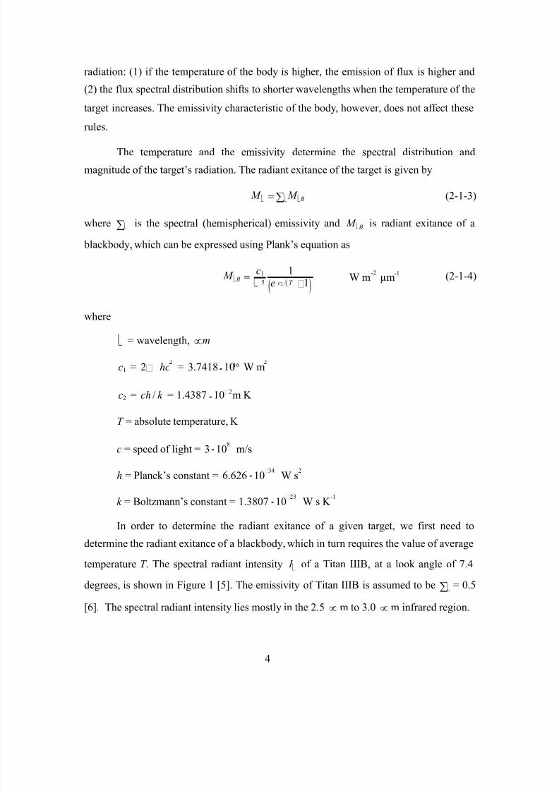
In order to determine the radiant exitance of a given target, we first need to determine the radiant exitance of a blackbody, which in turn requires the value of average temperature T . The spectral radiant intensity I of a Titan IIIB, at a look angle of 7.4 degrees, is shown in Figure 1 [5]. The emissivity of Titan IIIB is assumed to be = 0.5 [6]. The spectral radiant intensity lies mostly in the 2.5 m to 3.0 m infrared region.

4

7/28/2019 A 427181


S p e c t r a l I n t e n s i t y

( k W / s r -

m

T K (2-1-5)

T

60 50 40 30 20 10 0 2.0 2.5 3.0 3.5 4.0 4.5 5.0

Wavelength ( ) Figure 1. Spectral intensity of Titan IIIB at angle of attack of 7.4 deg (From Ref 5)

In Figure 1, the maximum intensity value occurs around peak = 2.8 m . The average temperature T of the target’s plume can then be calculated using Wien’s law as [7]:

2897.8 peak

where peak is the wavelength at which the peak value of spectral radiant intensity occurs (in m). From (2-1-5), for peak 2.8 m (see Figure 1), the target’s average temperature can be calculated as 1035 K.

From (2-1-3) and (2-1-4) and using T = 1035 K, the radiant exitance M of Titan IIIB is calculated and plotted as shown in Figure 2. By comparing the plots in Figures 1 and 2, the peak values in both cases occur at a wavelength of ~2.8 m as desired. If the radiant spectral intensity shown in Figure 1 is assumed to be due to just to the rocket plume, then by (2-1-1) the plume area can be approximated as

I 2.8m

L2.8m

I 2.8m

M 2.8m 600 m2 (2-1-6)

5

7/28/2019 A 427181


1.15 Wcm-2 . If we assume that the surface area of the plume as 600 m [8], then the

I P 550kWsr -

Figure 2. Radiant exitance of Titan IIIB (1035 K)

To calculate the radiant exitance within the detector band 2 2

M M d

M Bd 1 1

where the limits from Figure 2 are 1 3 m (2-1-7)

and 2 5 m , which gives 2

radiation intensity of the plume is M AT (2-1-8)

Before choosing the detector for the infrared sensor, we need to consider the effects of the atmosphere. The effects of the atmosphere are predominant for altitudes up to 15 km from the surface of the Earth. Although that is a small part of the boost phase, for early detection of the target launch, the atmospheric effects must be taken into account.

6

7/28/2019 A 427181


The atmosphere is made up of many different gases and aerosols. Some gases in

the atmosphere are: nitrogen, oxygen, argon, neon, carbon dioxide and water vapor. Aerosols include dirt, dust, sea salt, water droplets, and pollutants. The concentration of these gases differs from place to place. Most of the attenuation in the 2.5 m to 2.9 m region is caused by carbon dioxide and water vapor. Using a Searad model the atmospheric transmittance is calculated. In this model, we used 1976 US standard atmosphere, maritime extinction (visibility 23 km), air mass character (ICSTL) of 3, and no clouds or rain. The atmospheric transmittance results of the Searad calculations are shown in Figure 3. The atmospheric transmittance is not uniform for 3 m 5 m . Several absorption areas in the transmittance spectrum can be identified.

Figure 3. Atmospheric transmittance calculated using Searad From Figure 2, the plume energy is concentrated in the infrared region of about 2.8 m . Consequently, we may choose the midwave infrared region of 3-5 m for designing the

7

7/28/2019 A 427181


detector. Note that the transmittance plot in Figure 3 depicts some absorption about that wavelength.

The atmosphere not only affects the transmittance, but also affects the shape and size of the target plume. Because of the change in pressure and the concentration of the gases in the atmosphere, the size and shape of the plume changes with altitude. An example of these effects is shown in Figure 4 for the plume in the afterburning stage, the continuous flow regime, the molecular flow regime and the vacuum limit. The plume

Figure 4. The change of the plume at the atmosphere (From Ref 5) grows bigger with increasing altitude, and it gets smaller after it goes out of the atmosphere. The size of the plume diameter is about 10-100 meters at the beginning of the boost phase. At an altitude of 60 km (continuous flow regime) the diameter of the plume

begins

to

expand,

and

at an

altitude

of

160

km

(molecular

flow

regime)

it has

a

maximum diameter of 1-10 km. At 300 km, the diameter decreases to 1-10 m due to the vacuum limit. The change in radiance is shown in Figure 5 for the Titan IIIB for altitudes 18 km and 118 km.

Scale: 320x450 m (a)

Scale: 4.5 x 6.0 km (b)

Figure 5. Radiance map of Titan IIIB for MWIR at altitudes 18 km (a) and 118 km (b) (From Ref 5)

8

7/28/2019 A 427181


view (IFOV) of the detector d 2 and the focal length f 1 :

A typical side dimension for a square detector size is Ad 2 30 m . The diameter D of

2.44

Using a sensor design with focal length f 1 1.5 m gives d 2 =20 rad , and the diameter

For mixed terrain, the radiance of the background is L = 300 10 Wsr cm-2

[Ref 6, pg. 210]. For d 2 = 20 m and the satellite at RC = 1000 km above the ground, a footprint of 20 m 20 m square results in an area of 400 m . The total radiation

1

D I P I RC 2

SCR P S C D I C I C R P

2

2. Infrared Sensor Design The infrared sensors are low orbit staring type focal plane arrays on satellites. The

missile is a point target for the infrared sensors because of the large distance between the sensors and the target [2]. The detector area Ad depends on the instantaneous field of

1

Ad d f 12 m2 (2-1-9)

1 the sensor optics is calculated using diffraction as

D m (2-1-10) d 2 f 1

1 D = 24.4 cm.

6 -1 1

2 intensity becomes I C = 1.2 kWsr

-1 . Given these results, the signal-to-clutter ratio (SCR) can be expressed as

S T 4 R P 4 RC

(2-1-11)

where S T is the signal power from the target, S C is the clutter power, I P is the radiation intensity of the plume, I C is the radiation intensity of clutter, R P is the range between IR sensor and the plume, and RC is the range between IR sensor and the clutter.

9

7/28/2019 A 427181


SCR 26 dB

At launch, the initial SCR is estimated by setting range of the plume R P RC . We then have

I P 550 kW I C 1.2 kW

(2-1-12)

The SCR is high enough throughout the boost phase that we can assume that the infrared sensor will track the target continuously.

The most important infrared sensor parameter used in the fusion algorithm is the IFOV. The IFOV dictates the spatial resolution of each detector. The infrared sensor, the sensor’s field of view (FOV) and the IFOV are shown in Figure 6. The target missile’s plume and a footprint on the Earth are shown to be within the sensor’s IFOV.

SENSOR

IFOV MISSILE FOV

FOOTPRINT PLUME

Figure 6. Satellite with infrared sensor Infrared sensors are passive sensors. They give the azimuth and elevation

information of the target. The azimuth, elevation and range information are required to guide the intercept missile. To derive the target range information, the intersection of each infrared sensor’s IFOV is used. In Figure 7, the intersection area of two IFOVs is shown.

10

7/28/2019 A 427181


IR Sensor #1

IR Sensor #2

INTERSECTION VOLUME OF IFOVs

Figure 7. Intersection volume of infrared sensors. For the exact location of the satellites, the IFOV values of each sensor and the

azimuth and elevation angles to the target are assumed to be known. By using triangulation and the two intersecting IFOV cones, a volume can be derived that contains the target plume. As the target is a point source, the source area as seen by the sensor array can be anywhere within the detector area as illustrated in Figure 8. The detector will declare that there is a target regardless of source area’s position within the detector area. From this, we have the knowledge of the detector element that has the target image and the IFOV cone that contains the target. Additionally, the position of the IR satellite is known. The IFOV and the satellite position information are sent to the fusion center and used to find the intersection volume (as depicted in Figure 7) in order to determine the location of the ballistic missile.

11

7/28/2019 A 427181


IFOV

Mid line of IFOV Source area

Detector area Figure 8. Target area seen in the detector area

In the simulation, the true vector of target-to-satellite is determined. Then angles and from the satellite to the target are calculated. A random uniformly distributed error is added to the and angles. As the target must be within the IFOV lines, we choose the error value so that the midline of the IFOV can move up to IFOV / 2 radians. We repeat these steps for satellite number two. Now we have the midlines for both satellites. The target is within the intersection volume of these two IFOV cones. This volume is found and used in the sensor fusion algorithm to find the most probable location of the target. To determine the intersection volume, we search the points (in one meter increments) in the space to find which points are in both the IFOV cones to determine the intersection volume. These points are collected with their coordinates in a matrix. This matrix is the intersection volume matrix. Figure 9 illustrates the collection of points to form the intersection volume. The desired target is assumed to be present in this volume. The intersection volume matrix is shown in Figure 10.

12

7/28/2019 A 427181


our simulation), the footprint will be ~640 k m . In order to reduce the foot print size to

These points are only in one of the IFOV

This point is in both IFOV’s We put this points coordinates to the matrix

Sat #1

Sat #2

This point is not in either IFOV cones

Arbitrary points in space that we check if they are both in two IFOV cones Figure 9. Illustration of the process determining the intersection volume

True target position Points defining the intersection volume

Figure 10. Intersection volume matrix with true target position indicated The infrared sensor’s range to the target directly affects the size of the matrix. The

volume within the IFOV cone increases with range. If we use high earth orbit satellites (like Defense Support Program DSP satellites), for a given IFOV value (20 rad in

2

13

7/28/2019 A 427181


more reasonable values (footprint is around 400 m in this work), we choose low earth

T T RnP G G 4 maxkTBF

is the Boltzmann’s constant (1.38 10 J/deg ), B is the receiver’s input bandwidth, F is

BW

/S N (2-2-2)

T

2 orbit satellites (1000 km above Earth’s surface).

B.

RADAR

The forward based radar systems are operated in X-band with a low pulse repetition frequency (PRF). The reason an X-band radar is chosen is that the high resolution capability of this radar provides a good capability for tracking ballistic targets in the boost phase. The resolution capability of a radar is related to the beamwidth as given by [2]

Dr

where Dr is the antenna diameter. The other issue that has to be addressed is the unambiguous range Ru of the radar. The range Ru must be large enough to be able to track the target throughout the boost phase, which can be up to 2,000 km (for a liquid propellant ballistic missile).

1. Radar Equations The radar parameters determine the accuracy of the track information being

provided to the sensor fusion. The radar single pulse signal-to-noise ratio S / N required at the input to the receiver can be calculated as

3 4

where P is the peak power of the transmitter, n is the compression factor (n = 1 if no pulse compression is used) [6], GT and G R are the transmit and receive gains of the antenna, σ is radar cross section of the missile target, λ is the wavelength of the radar, k

23 the system noise factor, and L is the total loss. In our simulation, we assume that the

14

7/28/2019 A 427181


az el - -

antenna gain G R = GT . The bandwidth is B = 1/ where is the pulsewidth. The system noise temperature is 290 K and L is 1.

In the radar simulation, we add angular and range errors to the actual target position in order to generate the radar output. The noise added is Gaussian with its variance calculated for range and azimuth angle as

range c 1 2 k (2S / N ) N i (2-2-3)

B k (2S / N ) N i

where c is speed of light, B is the 3-dB beamwidth of the antenna, N i is the number of coherently integrated pulses, and k is the antenna error slope and is between 1 and 2 (for our scenario k = 1.7 for a monopulse antenna [6]).

The radar cross section of the ballistic missile plays an important role in sensing its position. From (2-2-2), S / N is directly proportional to the radar cross section of the ballistic missile. In (2-2-3) and (2-2-4), the variances of the range and angular errors are calculated using the S / N . Therefore, the radar cross section of the missile plays a significant role in the error variance. Figure 11 shows the radar cross section of a ballistic missile in X-band (10 GHz) for all four stages of the missile [9]. The fourth stage is the payload. The similarity of the radar cross section of the different stages is significant. Even as the length of the missile decreases (jettisoning the canisters), the radar cross section of the missile does not change appreciably. The lengths of the stages are shown in Table 1.

15

7/28/2019 A 427181


Figure 11. Radar cross section of the ballistic missile for four stages [From Ref 9]

Table 1. Length of the stages of Peacekeeper ballistic missile

16

Length of the stage Remaining length of the missile

Stage 1 8.175 m 21.8 m Stage 2 5.86 m 13.625 m Stage 3 2.3 m 7.765 m Stage 4 5.45 m 5.45 m

7/28/2019 A 427181


The beamwidth is 0.5 degrees, and the pulse repetition frequency is 150 Hz.

2. Radar Parameters The radar parameters used in the boost phase simulation are shown in Table 2.

The main issues that are taken into account in selecting these parameters are range and resolution. The pulsewidth assumed is 50 s , and the number of pulses integrated is 20.

Table 2. Radar parameters

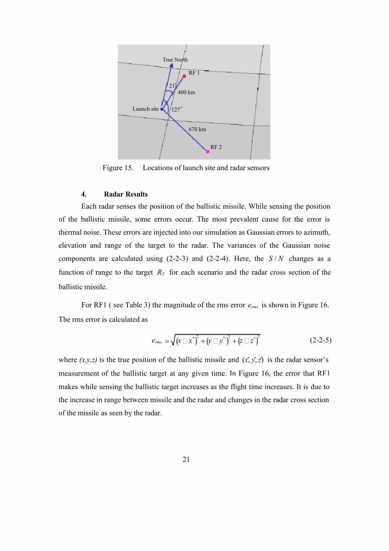
3. Position of Radar Sensors Positioning of the radar sensors play an important role in tracking the ballistic

missile target in the boost phase. During the travel of the ballistic missile, it is sensed from many different aspects by either radar. The continuous motion and change of aspects cause fluctuations in radar cross section of the ballistic missile. These fluctuations in radar cross section directly affect the results of the signal-to-noise ratio and the error of

17

Band X-band Frequency 10 GHz Peak power ( P T ) 500 kW Antenna diameter ( Dr ) 4.15 m Antenna efficiency ( ) 0.68 Antenna gain ( Gr Gt ) 50 dB Noise factor ( F ) 4 Number of pulses integrated ( N i ) 20 Beamwidth ( B ) 0.5 degrees Pulsewidth ( ) 50 s PRF ( F R ) 150 Hz

7/28/2019 A 427181


7/28/2019 A 427181


according to Figure 13 is 127 (the angle between true north, launch site and radar

the radar has changed to 95 with a range of 680-880 km; that is, the launch angle

Figure 13. Number of times S/N exceeds the threshold (headed to SF) 0

location) and 600-1000 km from launch site. If we locate the radar position corresponding to the peak values in this figure, the radar will track the missile closely for the entire boost phase. Since we do not know the exact heading of the missile, we have to examine other heading possibilities and check if the radar positions have their S / N exceed this threshold.

In Figure 14, the number of times the S / N of the radar exceeds the threshold is shown for a missile launched to hit Washington, DC. In Figure 14, the best position of

0 changes the best location for the radar sensors.

Using the simulation, we optimized the position of the radar systems; the best positions of the radar systems are listed in Table 3 (for both launch angles to San Francisco and Washington, DC). For optimization, we permutated the possible locations of the radar sensors and checked how many times both the radar sensors’ S / N exceeds

19

7/28/2019 A 427181


launch site and the radar sensors are shown in Figure 15.

Figure 14. Number of times SNR exceeds the threshold (headed to Washington) the threshold. As a result, the positions shown in Table 3 have one or both radar sensor’s S / N exceeding the threshold throughout the boost phase. The location of the

Table 3. Optimum radar positions (for launch angles to San Francisco and Washington, DC)

20

Angle between true north, launch site and radar

Distance between launch site and radar

RF1 21 degrees 400 km RF2 127 degrees 670 km

7/28/2019 A 427181


21

x xˆ2 y yˆ 2 z z ̂ 2 ˆ ˆ ˆ

True North RF 1

0 400 km

Launch site 127 0

670 km RF 2

Figure 15. Locations of launch site and radar sensors

4. Radar Results Each radar senses the position of the ballistic missile. While sensing the position

of the ballistic missile, some errors occur. The most prevalent cause for the error is thermal noise. These errors are injected into our simulation as Gaussian errors to azimuth, elevation and range of the target to the radar. The variances of the Gaussian noise components are calculated using (2-2-3) and (2-2-4). Here, the S / N changes as a function of range to the target RT for each scenario and the radar cross section of the ballistic

missile.

For RF1 ( see Table 3) the magnitude of the rms error erms is shown in Figure 16.

The rms error is calculated as erms (2-2-5)

where (x,y,z) is the true position of the ballistic missile and ( x, y, z ) is the radar sensor’s measurement of the ballistic target at any given time. In Figure 16, the error that RF1 makes while sensing the ballistic target increases as the flight time increases. It is due to the increase in range between missile and the radar and changes in the radar cross section of the missile as seen by the radar.

21

7/28/2019 A 427181


Figure 16. The rms error of RF1 (arbitrary position) For RF2, the rms error versus flight time plot is shown in Figure 17. The rms

Figure 17. The rms error of RF2 (arbitrary position) 22

7/28/2019 A 427181


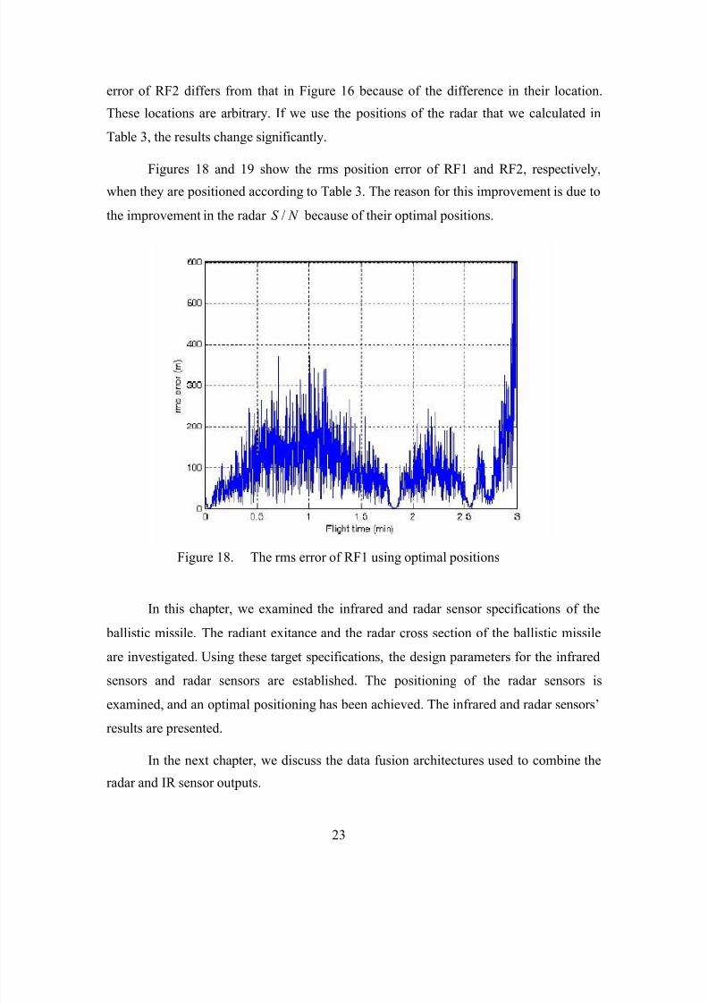
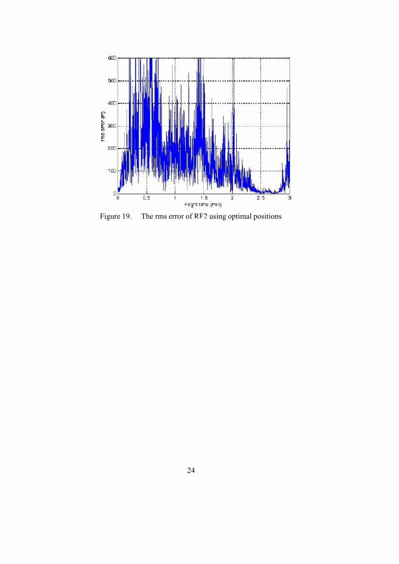
error of RF2 differs from that in Figure 16 because of the difference in their location. These locations are arbitrary. If we use the positions of the radar that we calculated in Table 3, the results change significantly.

Figures 18

and

19

show

the

rms

position

error

of

RF1

and

RF2,

respectively,

when they are positioned according to Table 3. The reason for this improvement is due to the improvement in the radar S / N because of their optimal positions.

Figure 18. The rms error of RF1 using optimal positions

In this chapter, we examined the infrared and radar sensor specifications of the ballistic missile. The radiant exitance and the radar cross section of the ballistic missile are investigated. Using these target specifications, the design parameters for the infrared sensors and radar sensors are established. The positioning of the radar sensors is examined, and an optimal positioning has been achieved. The infrared and radar sensors’ results are presented.

In the next chapter, we discuss the data fusion architectures used to combine the radar and IR sensor outputs.

23

7/28/2019 A 427181


Figure 19. The rms error of RF2 using optimal positions

24

7/28/2019 A 427181


7/28/2019 A 427181


according to the type of fusion processing used. The data fusion node performs the data alignment, data association and position or state estimation functions. The results of the data fusion are sent to a resource management function. The resource management function plans and controls the available resources (weapons, sensors, guidance and control, and process control) using the fused information and the user directives. The weapons and sensors are selected using the results of the resource management decisions. The response systems then react to the environment according to the resource management

In the following sections, two important functions of the model are discussed further: the data fusion node design and the fusion processing algorithms.

B. DATA FUSION NODE DESIGN The data fusion node performs three major functions: data alignment, data

association, and state estimation. Each of these is described below. 1. Data Alignment Data alignment also known as data preparation or common referencing [Ref 11,

pg. 16-30] changes or modifies the data that come from the sensors so that this data can be associated and compared. Data alignment modifies the sensor data to appropriate formats, and translates the information to the correct spatio-temporal coordinate system. It also compensates for the misalignments during changes between these dimensions.

Data alignment executes five processes that include common formatting, time propagation, coordinate conversion, misalignment compensation, and evidential conditioning. In the common formatting process, the data is being tested and transformed to system standard data units and types. The fused track data are updated to predict the expected location so that the new sensor inputs can be associated with them in the time propagation function. The data that come from separate sensors are converted to a common coordinate system. In this study, the coordinate systems for radars and infrared sensors are different from each other, but through data alignment they are converted to the Earth centric Cartesian coordinate system. In the misalignment compensation, the

26

7/28/2019 A 427181


data are corrected for the parallax between sensors. In the evidential conditioning, some confidence values are assigned to the data that come from each sensor [11].

2. Data Association In the data association function, the data that belong to the same target are

associated for improved position estimation. Data association is executed in three steps [11]: hypothesis generation, hypothesis evaluation and hypothesis selection. Using hypothesis generation, the solution space is reduced to a practical number. Feasibility gating of prior tracks or data clustering is used for hypothesis generation. Kinematic, parametric and a priori data are used for evaluating these hypotheses and a score is assigned to each hypothesis. The hypothesis selection uses these scores to select one or more sets of data to be used in the next step, which is state estimation. Data association is not used in this study since only one target is being tracked [11].

3. State Estimation The state estimation estimates and predicts the target position using the data that

come from data association. There are many algorithms to estimate the position of the target. The algorithms that we use in this study include averaging (arithmetic), weighting (using S / N ), Kalman filter and Bayesian techniques. These algorithms will be described in detail in Chapter IV.

C. PROCESSING ARCHITECTURES There are three basic architectures for multisensor data fusion: direct fusion of

feature vectors that are representations of sensor data, and decision level sensor fusion. 1. Direct Fusion Direct fusion uses raw data to fuse the sensor outputs. In Figure 21, the direct

fusion architecture is shown. The data received from the sensors are first subjected to the data association function. The associated data are then fused together. This is followed by the feature extraction operation. The results of the feature extraction block are then sent to position estimation. These fused positions are sent to the resource management, and guidance and control unit guides the interceptor missile to intercept the ballistic missile.

27

7/28/2019 A 427181


F e a t u r e

e x

t r a c t i o n

F e a t u r e

e x

t r a c t i o n

D a t a l e

v e l f u

s i o n

D a t a l e

v e l f u

s i o n

J o i n

t D e c i s i o n

A s s o c i a

t i o n

Data Fusion node

Sensor#1

Sensor#2

Sensor#3

Sensor#4

Figure 21.

Direct

level

fusion

(After

Ref

11,

pg.

1-7)

Direct fusion has the potential to achieve the best target position estimation. Another advantage of direct fusion is that, at the end of the fusion process, the targets can be detected even if the sensors cannot detect the target by themselves individually.

Direct fusion architecture gives the best results, but it also has some disadvantages. The data flow from the sensors to the fusion center is large, and the bandwidth needs are great. Direct fusion has the highest computational effort. With this fusion architecture, position estimations are based on the information from the sensors by evaluating the raw data. The registration accuracies play an important role, so direct fusion is very sensitive to registration errors. The sensors are required to be the same or similar; in this work, they are not. Since a variety of sensors (passive infrared sensors and active radar sensors) are used in this thesis in a ballistic missile interception task, the direct fusion architecture is not considered.

2. Feature Level Fusion Feature level fusion combines the features of the targets that are detected in the

each sensor’s domain. In Figure 22, the feature level fusion architecture is shown. The sensors must detect the targets in advance to be able to use this fusion process. The sensors extract the features for each target, and these features create a feature space for target detection [12]. The sensors process and extract the features of the measurement

28

7/28/2019 A 427181


A s s o c i a

t i o n

F e a t u r e l e

v e l f u

s i o n

J o i n

t D e c i s i o n

J o i n

t D e c i s i o n

outputs individually and then these processed data are sent to the association module in the fusion center. After the data are associated, they are fused in the feature level fusion center. A joint decision is formed and sent to the resource management module.

Data Fusion node Sensor#1 Processing/

Feature extraction Sensor#2 Processing/

Feature extraction Sensor#3 Processing/

Feature extraction

Sensor#4 Processing/ Feature extraction Figure 22. Feature level fusion (After Ref 11, pg. 1-7)

This type of fusion reduces the demand on registration, and the bandwidth required for the data to flow from each sensor to the fusion center is low compared to direct fusion.

This kind of fusion is often used for infrared sensors, but in ballistic missile interception missions all the sensors are not infrared. The features that the radar sensors and infrared sensors extract are different (infrared sensors use the plume temperature while the radar sensors use the radar cross section of the ballistic missile). As a result, we do not use this kind of fusion processing in this work.

3. Decision Level Fusion Decision level fusion combines the local decisions of independent sensors. The

decision level

fusion

architecture

is

shown

in

Figure

23.

For

this

kind

of

fusion

process,

the sensors must make preliminary decisions. The raw data in the sensors are processed in the sensor, and only the results that have the position estimation of the ballistic missile are sent to the fusion center. In the fusion center, the processed position data of the ballistic missile are associated. This associated data are then fused to achieve more

29

7/28/2019 A 427181


D e c i s i o n l e

v e l f u

s i o n

D e c i s i o n l e

v e l f u

s i o n

J o i n

t D e c i s i o n

A s s o c i a

t i o n

accurate position estimation. The fused data are sent to the resource management module, and the interceptor is guided accordingly.

Data Fusion node Sensor#1

Sensor#2

Sensor#3

Sensor#4

Processing

Processing

Processing

Processing

Figure 23. Decision level fusion (After Ref 11, pg. 1-7)

This data fusion process is less sensitive to spatial misregistration than the direct and feature level fusion approaches [11]. That is, it allows a more accurate association of the targets that contain registration errors. One of the advantages of this type of data fusion is the simplicity of adding and subtracting the sensors to the fusion system. The variety of the sensors does not affect the results from this fusion architecture.

In this chapter, the JDL fusion model is considered. The data fusion node design and the data alignment, data association, and state estimation functions of the fusion node are described. Direct fusion, feature level fusion, and decision level fusion architectures are described, and their relative advantages and disadvantages for the ballistic missile intercept in the boost phase are presented. The decision level fusion is selected as the architecture for the algorithms described in Chapter IV.

30

7/28/2019 A 427181


1 x1, y1, z 1 p2 x2 , y2 , z 2 ˆ a ( x, y, z ) (4-1-1)

ˆ ˆ ˆ

IV DECISION LEVEL FUSION ALGORITHMS

A decision level fusion architecture is used in the simulation. Below, the decision level fusion algorithms examined are described. They include an averaging technique, a weighted averaging technique, a Kalman filtering, and a Bayesian technique.

A. AVERAGING TECHNIQUE The first fusion algorithm investigated is an averaging technique. The sensors

process their own data and they send these decisions to the fusion center. In this work, this data is the position of the ballistic missile sensed by each sensor. The averaging technique computes the fused position as an arithmetic mean using the formula

2 where pa ( x, y, z ) is the position estimation of the averaging technique, and p1 x1, y1, z 1 and p2 x2 , y2 , z 2 are the position estimations of RF1 and RF2, respectively.

An example of the sensed positions from both RF1 and RF2 are shown in Figure 24. In Figure 24, the target’s true position, estimated positions as sensed by RF1 and

Figure 24. True target position, sensed positions by radars and arithmetic mean of sensed positions of the target

31

7/28/2019 A 427181


RF2, and the arithmetic mean of the sensed positions are shown at an arbitrary time instant. The RF1 sensor senses the target with a 158-m position error, RF2 sensor senses it with a 64-m error, and the fused or arithmetic mean position is 95 m away from true target position. In this case, however, the fused position of the target is worse than RF2 results. This situation, however, is not always true. For example, if the magnitude of the sensed position by one radar is opposite that of the other radar’s, then the arithmetic mean position will be better than that given by either of the radars individually.

We examine the cumulative error sensed by the radars and also the arithmetic mean position through simulation. The rms error computed using (2-2-5) of RF1 and RF2 obtained from MATLAB simulation are shown in Figure 25. The arithmetic mean of these errors is shown in Figure 26. We observe that the cumulative position estimation error of RF1 is the worst of all; the results of the arithmetic mean position are better than the RF2’s results, but RF1 gives the best results among these three.

(a) (b) Figure 25. The rms error of (a) RF1 and (b) RF2

32

7/28/2019 A 427181


7/28/2019 A 427181


ˆ ˆ

ˆ ˆ

ˆ

B. WEIGHTED AVERAGING TECHNIQUE The next sensor fusion algorithm that we investigate is the weighted average

method. In this algorithm, the sensors process their own data and send these decisions to the fusion center. These decisions are the positions of the ballistic missile sensed by each sensor.

The weighted average algorithm is similar to the averaging method; however, in weighted average method, we weigh the sensor data by using the radar sensors’ S / N for every time sample. The S / N for the radar sensors are calculated using (2-2-2). In the weighted average algorithm, the higher the S / N , the larger the weight for that target estimate. The weighted average of the target position is calculated using

pw ( x, y, z ) p1( x1, y1, z 1) (S / N )1

p2 ( x2 , y2 , z 2 ) (S / N )2 (S / N )1 (S / N )2 (4-2-1)

where pw ( x, y, z ) is the fused target position vector using weighted averaging technique, p1( x1, y1, z 1) is the position vector of the target sensed by RF1, (S / N )1 is the signal to noise ratio of RF1, p2 ( x2 , y2 , z 2 ) is the position vector of the target sensed by RF2, and (S / N )2 is the signal to noise ratio of RF2.

An example of these sensed and weighted average positions is shown in Figure 27. In this example, RF1 senses the target with a 125-m position error, RF2 senses the same target with a 44-m error, and the weighted average position is 36 m away from the true target position. The fused position of the target is better than both radar sensor results.

The cumulative error sensed by the radars is examined, and the weighted average position computed in a MATLAB simulation. We observe that the cumulative position estimation error for the weighted averaging technique is better than that of both radars. The rms error plots of the radar sensors are shown again in Figure 28. The results of the weighted averaging technique are shown in Figure 29. By comparing the results of Figure 28 and 29, the weighted averaging technique provides the best position estimate among the three plots.

34

7/28/2019 A 427181


1

Figure 27. True target position, sensed positions by radars and weighted averaging position of the target

(a) (b) Figure 28. The rms error of (a) RF1 and (b) RF2

35

7/28/2019 A 427181


Figure 29. The rms error of weighted averaging technique estimation of target position The average rms errors erms , computed as given by (4-1-2), are shown in Table 5.

For the averaging technique (see Table 4), the average rms error was 102 m., which was worse than that of RF1. The weighted averaging technique provides a significant improvement

over

these

results.

The

average

error

due

to

weighted

averaging

technique

is 68 m.

Table 5. Average rms error for radar sensors and weighted averaging technique

36

erms in m RF1 99 RF2 157 Weighted averaging technique. 68

7/28/2019 A 427181


7/28/2019 A 427181


P (t | t ) K (t ) RK (t )T I K (t ) H (t ) P (t | t 1) I K (t ) H (t )

ˆ ˆ ˆ

ˆ

ˆ

r ˆ ˆ

P (t | t 1) F (t 1) P (t 1| t 1) F (t 1)T Q(t 1) , (4-3-6)

the Kalman gain can be calculated using the following formula: K (t ) P (t | t 1) H (t )T H (t ) P (t | t 1) H (t )T R(t ) 1

(4-3-7) The equation of the optimum estimate of the ballistic missile state vector is given by

x(t | t ) x(t | t 1) K (t ) z (t ) H (t ) x(t | t 1) and the update for the error covariance update is

T

(4-3-8)

(4-3-9) By repeating the equations recursively, the updated state estimations can be found.

The Kalman filter processes the measurements coming from the sensors in real time and smooths the outputs of the radar sensors’ range, elevation and azimuth information to obtain better target position estimates. Error in range r , elevation , and azimuth are computed using

r err r r err

err

(4-3-10)

where ( r err , err , err ) are error components, ( r , , ) are true values, and ( ˆ, , ) are the measurements (sensor data) or estimates of the Kalman filter. The Kalman filtered range, elevation, and azimuth error of RF1 are shown in Figure 30. The blue lines represent the error for the range, elevation, and azimuth sensed by the RF1. The black line is the Kalman filtered error for the azimuth, elevation, and range for RF1. By using the Kalman filter, the fluctuations of the error have been reduced significantly in all three plots.

The rms position error for RF1 can be computed by first converting from the spherical to the Cartesian coordinates and then using (2-2-5). The rms position errors for sensor data (blue line) and Kalman filtered data (black line) are shown in Figure 31.

38

7/28/2019 A 427181


e r r o r ( m )

e r r o r ( r a d i a n s )

e r r o r ( r a d i a n s )

Clearly, the Kalman filter helps reduce the rms position error. Next, the Kalman filtered position estimates for both RF1 and RF2 will be fused using weighted averaging.

(a) (b)

(c) Figure 30. Kalman filtered errors for RF1: (a) range, (b) elevation and (c) azimuth

39

7/28/2019 A 427181


Figure 31. Overall position error after using Kalman filter for RF1 Figure 32 shows the range, elevation, and azimuth error plots for sensor data

(blue) and Kalman filtered data (black) for RF2. The fluctuations of the rms error diminished in all three plots. Figure 33 shows the rms position error for sensor (blue) and Kalman filtered (black) data. As in Figure 31, the Kalman helps reduce the rms position error of RF2 significantly.

40

7/28/2019 A 427181


7/28/2019 A 427181


To fuse the Kalman filtered radar sensor outputs, the weighted averaging

technique is used. The rms error of the Kalman filtered and sensor data are combined using (4-2-1). The signal-to-noise ratios are used for weighing the Kalman filtered RF1 and RF2 outputs. Weighted average results of the Kalman filtered rms error are shown in Figure 34.

Figure 34. The rms error for weighted averaging technique after RF1 and RF2 outputs are Kalman filtered

Table 6 lists the average rms errors erms for RF1, RF2, and the weight averaged Kalman filtered errors. The average error for Kalman filtering is 52 m, which is about half that of RF1 and one third that of RF2. From Table 4, recall that the averaging technique has produced an average rms error of 102 m. From Table 5, the weighted averaging technique has produced an average rms error of 68 m. The Kalman filtered algorithm is clearly better than those two algorithms.

42

7/28/2019 A 427181


7/28/2019 A 427181


7/28/2019 A 427181


7/28/2019 A 427181


7/28/2019 A 427181


V. CONCLUSION

In this thesis, the multiple sensor fusion in the boost phase of a ballistic missile intercept is examined. Measurements of RF and IR sensors are considered for fusion here. The fused sensor outputs lead to better guidance of the intercept missile and tracking of the ballistic missile. A MATLAB simulation is used to model the ballistic missile and the infrared and radar sensors. Four different data fusion algorithms are simulated and their results compared. A. CONCLUSIONS

From the results of the IR sensor analysis, in the designing of infrared sensors, 3 m to 5 m band should be used for detecting and tracking the ballistic missile. The infrared sensor satellites should be low earth orbit (LEO) satellites as the higher orbital satellites increase the IFOV intersection volume. The signal-to-clutter ratio, which plays an important role in detecting the ballistic missile, must be high enough to detect and track the ballistic missile for the entire boost phase. In this thesis, the triangulation of the instantaneous field of view for the infrared sensors is used to obtain the range information.

For the radar sensors, the positions of the radar sensors play an important role in detecting and tracking the ballistic missile.

The decision level fusion for combining the sensor outputs is considered in this work. Four sensor fusion algorithms are investigated. In the averaging technique, the fused results are not always better than these of the individual sensor outputs. The weighted averaging technique performs better than the averaging technique. The Kalman filtering approach helps decrease the sensor rms errors significantly. The Bayesian technique has the best performance of all four fusion algorithm investigated here. B. RECOMMENDATIONS

This thesis investigated a single target scenario. In a future study, fusion algorithms for intercepting multiple ballistic missiles in the boost phase may be investigated. The issues of association and correlation need to be addressed.

47

7/28/2019 A 427181


In this thesis, the interceptor missile is not included; only the detection, tracking

and position estimation of the ballistic missile is studied. In a future study, the effects of sensor fusion on the interceptor missile’s kill vehicle effectiveness may be quantified.

The ballistic

missile

may

use

electronic

attack

techniques,

such

as jamming,

throughout the boost phase. The effects of electronic attack on fusion performance may be studied in a future work.

48

7/28/2019 A 427181


APPENDIX MATLAB CODES

The MATLAB codes to simulate the sensors, ballistic missile and compute the algorithms are included in this appendix.

%gokhan humali 2004 NPS %sensor fusion for boost phase interception of ballistic missile

clear; clc;

%Constants Re = 6371e3; %Earth radius (m) Me = 5.9742e24; %Earth mass (kg) Gc = 6.673e-11; %Gravitational constant (m^3 kg^-1 s^-2) g0 = Gc * Me / (Re ^ 2); %Gravitational Acceleration (sea level) c = 299792458; %Speed of light (m/s)

t = 0; %Time (s) dt = 0.1; %Time increment (s)

posEarth = [0; 0; 0]; %Earth's center position

degRad = pi/180; %Degree to Radian conversion

%target information balMisLatH = 'N'; %Bal. Mis. launch site latitude hemisphere balMisLatD = 41; %Bal. Mis. launch site latitude (degree) balMisLatM = 00; %Bal. Mis. launch site latitude (minute)

balMisLonH = 'E'; %Bal. Mis. launch site longitude hemisphere balMisLonD = 129; %Bal. Mis. launch site longitude (degree)

49

7/28/2019 A 427181


7/28/2019 A 427181


7/28/2019 A 427181


velBM = magVelBM * unBMvel; %velocity of ballistic missile grndTrckBM = posBM; %ground track of BM %target information ends

%infrared sensor information hIR1 = 1000e3; %Height of infrared sensor 1 (above ground) (m) hIR2 = 1000e3; %Height of infrared sensor 2 (above ground) (m)

IR1LatH = 'N'; %infrared sensor (IR1) latitude hemisphere IR1LatD = 36; %IR1 latitude (degree) IR1LatM = 00; %IR1 latitude (minute)

IR1LonH = 'E'; %IR1 longitude hemisphere IR1LonD = 132; %IR1 longitude (degree) IR1LonM = 00; %IR1 longitude (minute)

IR2LatH = 'N'; %infrared sensor (IR2) latitude hemisphere IR2LatD = 46; %IR2 latitude (degree) IR2LatM = 00; %IR2 latitude (minute)

IR2LonH = 'E'; %IR2 longitude hemisphere IR2LonD = 132; %IR2 longitude (degree) IR2LonM = 00; %IR2 longitude (minute)

%change the geographical coordinates of the IR sensors to cartesian [thetaIR1 phiIR1] = geo2sph(IR1LatH, IR1LatD, IR1LatM, IR1LonH, IR1LonD,

IR1LonM); [xIR1,

yIR1,

zIR1]

=

sph2car(thetaIR1,

phiIR1,

(Re

+

hIR1));

posIR1 = [xIR1; yIR1; zIR1];

[thetaIR2 phiIR2] = geo2sph(IR2LatH, IR2LatD, IR2LatM, IR2LonH, IR2LonD, IR2LonM);

[xIR2, yIR2, zIR2] = sph2car(thetaIR2, phiIR2, (Re + hIR2)); 52

7/28/2019 A 427181


posIR2 = [xIR2; yIR2; zIR2];

IFOV1 = 20e-6; %IFOV of infrared sensor #1 IFOV2 = 20e-6; %IFOV of infrared sensor #2 %infrared sensor information ends

%Ballistic Missile RCS information for X band radar (from kuzun thesis) load POstage1_X; %load rcs data of bal. mis. for stage 1 (x band) balMisRCSstg1X = Sth; load POstage2_X; %load rcs data of bal. mis. for stage 2 (x band) balMisRCSstg2X = Sth; load POstage3_X; %load rcs data of bal. mis. for stage 3 (x band) balMisRCSstg3X = Sth; load POstage4_X; %load rcs data of bal. mis. for stage 4 (x band) balMisRCSstg4X = Sth;

rcsOrgAngMono = 0:360; %angle incriments in the original rcs table rcsInc = 0:0.1:360; %angle incriments for interpolation

%interpolation of rcs data to 0.1 degrees increments rcsXstg1 = interp1(rcsOrgAngMono, balMisRCSstg1X, rcsInc); rcsXstg2 = interp1(rcsOrgAngMono, balMisRCSstg2X, rcsInc); rcsXstg3 = interp1(rcsOrgAngMono, balMisRCSstg3X, rcsInc); rcsXstg4 = interp1(rcsOrgAngMono, balMisRCSstg4X, rcsInc);

%radar sensor information RF1LatH = 'N'; %radar sensor 1 (RF1) latitude hemisphere RF1LatD = 44; %RF1 latitude (degree) RF1LatM = 34; %RF1 latitude (minute)

RF1LonH = 'E'; %RF1 longitude hemisphere RF1LonD = 130; %RF1 longitude (degree) RF1LonM = 48; %RF1 longitude (minute)

53

7/28/2019 A 427181


RF2LatH = 'N'; %radar sensor 2 (RF2) latitude hemisphere RF2LatD = 37; %RF2 latitude (degree) RF2LatM = 21; %RF2 latitude (minute)

RF2LonH = 'E'; %RF2 longitude hemisphere RF2LonD = 135; %RF2 longitude (degree) RF2LonM = 04; %RF2 longitude (minute)

%change the geographical coordinates of the radar sensors to cartesian [thetaRF1 phiRF1] = geo2sph(RF1LatH, RF1LatD, RF1LatM, RF1LonH, RF1LonD,

RF1LonM); [xRF1, yRF1, zRF1] = sph2car(thetaRF1, phiRF1, Re); posRF1 = [xRF1; yRF1; zRF1];

[thetaRF2 phiRF2] = geo2sph(RF2LatH, RF2LatD, RF2LatM, RF2LonH, RF2LonD, RF2LonM);

[xRF2, yRF2, zRF2] = sph2car(thetaRF2, phiRF2, Re); posRF2 = [xRF2; yRF2; zRF2];

%radar sensor specifications PtR1 = 1e6; %RF1 peak power (w) PtR2 = 1e6; %RF2 peak power (w) DR1 = 4.15; %RF1 antenna diameter (m) DR2 = 4.15; %RF2 antenna diameter (m) fR1 = 10e9; %RF1 frequency (Hz) fR2 = 10e9; %RF2 frequency (Hz) roR1 = 0.68; %RF1 antenna efficiency roR2 = 0.7; %RF2 antenna efficiency tauR1 = 50e-6; %RF1 pulsewidth tauR2 = 50e-6; %RF2 pulsewidth FR1 = 4; %RF1 noise figure FR2 = 4; %RF2 noise figure

54

7/28/2019 A 427181


nR1 = 20; %RF1 # of pulses being integrated nR2 = 20; %RF2 # of pulses being integrated kT0 = 4e-21; %Watts/Hz kAng = 1.7; %k value for angle kRan = 1.7; %k value for angle lamR1 = c ./ fR1; %wavelength of RF1 lamR2 = c ./ fR2; %wavelength of RF2 AeR1 = pi .* ((DR1 ./ 2) ^ 2); %RF1 antenna physical area AeR2 = pi .* ((DR2 ./ 2) ^ 2); %RF2 antenna physical area GR1 = (4 * pi * roR1 * AeR1 / (lamR1 ^ 2)); %RF1 antenna gain GR2 = (4 * pi * roR2 * AeR2 / (lamR2 ^ 2)); %RF2 antenna gain beamWR1Deg = 65 * lamR1 / DR1; %RF1 beamwidth (degree) beamWR2Deg = 65 * lamR2 / DR2; %RF2 beamwidth (degree) beamWR1 = beamWR1Deg * degRad; %RF1 beamwidth (radian) beamWR2 = beamWR2Deg * degRad; %RF2 beamwidth (radian) %radar sensor information ends

%initial values for misc variables magDiffBM_RF1 = 0; %mag of dif of true BM position and sensed pos. by RF1 magDiffBM_RF2

=

0;

%mag

of

dif

of

true

BM

position

and

sensed

pos.

by

RF2

magDifAritMean = 0; %mag of dif of true BM pos and arit mean of RF1 and RF2 results magDifWeiAve = 0; %mag of dif of true BM pos and weighted ave of RF1 and RF2 results magDifWeiIR = 0; %mag of dif of true BM pos and weighted ave of RF1 and RF2 in IR volume

%Arrays timeArr = []; %Simulation time array posArrBM = []; %Ballistic missile position array grndTrckArrBM = []; %Ballistic missile ground track array distArrBM = []; %Ballistic missile ground distance array velArrBM = []; %Ballistic missile velocity array

55

7/28/2019 A 427181


difArrBM_RF1 = []; %Array of difference between true pos of BM and RF1 sensed difArrBM_RF2 = []; %Array of difference between true pos of BM and RF2 sensed difAritMeanBM_RF = []; %Array of diff between true pos of BM and arit mean of RF sensor outputs difWeiArrBM_RF = []; %Array of diff between true pos of BM and weighted ave. pos of RF sensor outputs difWeiArrIR = []; %Array of diff between true pos of BM and weighted ave pos of RF sensor outputs using IR volume

flag1 = 1;

while t < nexStgTime4 %assign ISPT and dMdt values for each stage if t < nexStgTime2

if flag1 == 1 ISPT = balMisISPstg1; dMdt = dMdtStg1; flag1 = 2;

end stageBM = 1;

elseif (nexStgTime2 <= t) & (t < nexStgTime3) if flag1 == 2

totMass = totMass - canWeiStg1; ISPT = balMisISPstg2; dMdt = dMdtStg2; flag1 = 3;

end stageBM = 2;

elseif (nexStgTime3 <= t) & (t < nexStgTime4) if flag1 == 3

totMass = totMass - canWeiStg2; ISPT = balMisISPstg3; dMdt = dMdtStg3;

56

7/28/2019 A 427181


flag1 = 4;

end stageBM = 3;

else totMass = totMass - canWeiStg3; ISPT = balMisISPstg4; dMdt = dMdtStg4; stageBM = 4;

end

%magnitude of position vector of Ballistic missile magPosBM = sqrt(posBM(1) ^ 2 + posBM(2) ^ 2 + posBM(3) ^ 2); %unit vector of ballistic missile position vector unPosBM = posBM / magPosBM; gBM = (Gc * Me) / (magPosBM ^ 2); %gravitational acceleration of BM

velBM = velBM + accBM * dt; %velocity vector of BM %magnitude of velocity vector of BM magVelBM = sqrt(velBM(1) ^ 2 + velBM(2) ^ 2 + velBM(3) ^ 2); unBMvel

=

velBM

/ magVelBM;

%unit

vector

of

vel

vec

of

BM

magWeiBM = totMass * gBM; %magnitude of weight vector of ball missile unMagWeiBM = -unPosBM; %unit vec of weight vector of ball missile weiVec = unMagWeiBM * magWeiBM; %weight vector of ballistic missile

magThrBM = dMdt * gBM * ISPT; %magnitude of thrust vector of ball missile unThrBM = unBMvel; %unit vector of thrust vec of ball missile thrBM = magThrBM * unThrBM; %thrust vector of ballistic missile totForceBM = weiVec + thrBM; %total force on ballistic missile accBM = totForceBM / totMass; %acceleration of ballistic missile

totMass = totMass - dMdt * dt; %total mass of the ballistic missile 57

7/28/2019 A 427181


7/28/2019 A 427181


RCS2 = rcsXstg3(RF2RCSIndex);

else RCS1 = rcsXstg4(RF1RCSIndex); RCS2 = rcsXstg4(RF2RCSIndex);

end

vecBM_RF1 = posBM - posRF1; %Vector between Ballistic missile and RF1 %Magnitude of Ballistic missile - RF1 vector magBM_RF1 = sqrt((vecBM_RF1(1) ^ 2) + (vecBM_RF1(2) ^ 2) +

(vecBM_RF1(3) ^ 2)); %True angle between Ballistic missile and RF1 trueAngBM_RF1 = atan2(vecBM_RF1(2), vecBM_RF1(1));

vecBM_RF2 = posBM - posRF2; %Vector between target and RF2 %Magnitude of Ballistic missile - RF2 vector magBM_RF2 = sqrt((vecBM_RF2(1) ^ 2) + (vecBM_RF2(2) ^ 2) +

(vecBM_RF2(3) ^ 2)); %True angle between Ballistic missile and RF2 trueAngBM_RF2 = atan2(vecBM_RF2(2), vecBM_RF2(1));

SNR1 = PtR1 * (GR1^2) * (lamR1 ^2) * (10^(RCS1 / 10)) * tauR1 / (((4 * pi) ^3) * kT0 * FR1 * (magBM_RF1 ^ 4)); %SNR of RF1

SNR2 = PtR2 * (GR2^2) * (lamR2 ^2) * (10^(RCS2 / 10)) * tauR2 / (((4 * pi) ^3) * kT0 * FR2 * (magBM_RF2 ^ 4)); %SNR of RF2

%Sigma of angle error of RF1 sigAngleRF1 = beamWR1 / (kAng * sqrt(2 * SNR1 * nR1)); %Sigma of angle error of RF2 sigAngleRF2 = beamWR2 / (kAng * sqrt(2 * SNR2 * nR2)); errAzRF1 = sigAngleRF1 * randn; %Erroneous angle for RF1 errAzRF2 = sigAngleRF2 * randn; %Erroneous angle for RF2

errElRF1 = sigAngleRF1 * randn; %Erroneous angle for RF1 59

7/28/2019 A 427181


7/28/2019 A 427181


7/28/2019 A 427181


7/28/2019 A 427181


7/28/2019 A 427181


7/28/2019 A 427181


grid

%figure of true bal mis position and shifted position using IR (weighted) figure plot((timeArr / 60), difWeiArrIR); title('True bal mis position vs. final algorithm weighted(RF1, RF2, IR1, IR2)'); xlabel('Flight time (min)'); ylabel('rms error (m)'); axis([0 3 0 600]); grid

%figure of infrared intersection volume and bal mis figure for i = 1:size(volArray,2)

plot3(volArray(1,i), volArray(2,i), volArray(3,i)); hold on

end axis square plot3(posBM(1), posBM(2), posBM(3), 'or')

disp(['Sum of errors of dif between bal mis and sensed by RF1 =' num2str(sum(difArrBM_RF1)) ' m']);

disp(['Sum of errors of dif between bal mis and sensed by RF2 =' num2str(sum(difArrBM_RF2)) ' m']);

disp(['Sum of errors of dif between bal mis and arithmetic mean position =' num2str(sum(difAritMeanBM_RF)) ' m']);

disp(['Sum of errors of dif between bal mis and weighted position =' num2str(sum(difWeiArrBM_RF)) ' m']);

disp(['Sum of errors of dif between bal mis and final algorithm (wei) =' num2str(sum(difWeiArrIR)) ' m']);

65

7/28/2019 A 427181


7/28/2019 A 427181


%gokhan humali 2004 %conversion of geographic coordinates to spherical coordinates

function [thet, phi] = geo2sph(latH, latD, latM, lonH, lonD, lonM)

deg2rad = pi / 180; latDegree = latD + latM / 60; latRad = latDegree * deg2rad;

lonDegree = lonD + lonM / 60; lonRad = lonDegree * deg2rad;

if latH == 'N' thet = pi / 2 - latRad;

elseif latH == 'S' thet = pi / 2 + latRad;

end

if lonH == 'E' phi

=

lonRad;

elseif lonH == 'W'

phi = 2 * pi - lonRad; end

%gokhan humali 2004 %conversion of spherical coordinates to cartesian coordinates

function [x, y, z] = sph2car(thet, phi, R) x = sin(thet) * cos(phi) * R; y = sin(thet) * sin(phi) * R; z = cos(thet) * R;

67

7/28/2019 A 427181


%gokhan humali 2004 %excitance of the ballistic missile plume at temperature T

clear;clc;

lam=linspace(1,14,1000); h = 6.625e-34; c = 3e8; k = 1.38e-23; T = 1035; emissivity = 0.5; c1 = 3.7417749e4; c2 = 1.4387e4;

gh = exp(h.*c./(lam.*k.*T));

M = c1 ./ (lam .^ 5 .* (exp(c2./(lam.*T))-1));

figure plot(lam,M*1e4)

%multiply

with

1e4

to

convert

the

result

to

m^-2

xlabel('Wavelength (micrometer)') ylabel('Radiant exitance of blackbody (W/(m^2 micrometer))') grid

figure plot(lam,M*emissivity*1e4) xlabel('Wavelength (micrometer)') ylabel('Radiant exitance of graybody (W/(m^2 micrometer))') grid

68

7/28/2019 A 427181


%gokhan humali 2004 %computes the midline of the infrared sensor's IFOV.

function errTIR = midIRline(posTar, posIR, IFOV)

flag = 1; vecTIR = posTar - posIR; %vector from IR sat. to ballistic missile %magnitude of the vector between IR sat. and ballistic missile magVecTIR = sqrt(vecTIR(1) ^ 2 + vecTIR(2) ^ 2 + vecTIR(3) ^ 2); %theta angle for the vector between IR sat. and bal. mis. theta = atan2(vecTIR(2), vecTIR(1)); %phi angle for the vector between IR sat. and bal. mis. phi = acos(vecTIR(3) / magVecTIR);

while flag ran_1 = rand - 0.5; %first random number between -0.5 to 0.5 ran_2 = rand - 0.5; %second random number between -0.5 to 0.5 %components of the new vector between IR sat. and bal. mis. with adding random

number times IFOV x = magVecTIR * cos(theta + ran_1 * IFOV) * sin(phi + ran_2 * IFOV); y = magVecTIR * sin(theta + ran_1 * IFOV) * sin(phi + ran_2 * IFOV); z = magVecTIR * cos(phi + ran_2 * IFOV); errTIR = [x; y; z]; magErrTIR = sqrt(errTIR(1) ^ 2 + errTIR(2) ^ 2 + errTIR(3) ^ 2);

%check the new vector if it is really inside IFOV/2 a = dot(errTIR, vecTIR); b

=

magErrTIR

*

magVecTIR;

d = acos(a / b); if (d <= (IFOV / 2))

flag = 0; end

end 69

7/28/2019 A 427181


%gokhan humali 2004 %conversion of topographic coordinates to cartesian coordinates [After kuzun thesis]

function [x, y, z] = top2car(az, el, latH, latD, latM, lonH, lonD, lonM)

deg2rad = pi / 180; if latH == 'N'

lat = (latD + latM / 60) * deg2rad; elseif latH == 'S'

lat = -(latD + latM / 60) * deg2rad; end

if lonH == 'E' lon = (lonD + lonM / 60) * deg2rad;

elseif lonH == 'S' lon = -(lonD + lonM / 60) *deg2rad;

end

HA = sin(el); EA

=

cos(el)

*

cos(az);

NA = cos(el) * sin(az);

%Rotation vector T = [ -sin(lat)*cos(lon) -sin(lon) cos(lat)*cos(lon)

-sin(lat)*sin(lon) cos(lon) cos(lat)*sin(lon) cos(lat) 0 sin(lat) ];

solVec = [0; 0; 0]; solVec = T * [EA; NA; HA];

x = solVec(1); y = solVec(2); z = solVec(3);

70

7/28/2019 A 427181


%gokhan humali 2004 %IR intersection volume function volArr = volumeIR(posTar, positIR1, positIR2, errorTIR1, errorTIR2, IFOV_1, IFOV_2)

magErrTIR1 = sqrt(errorTIR1(1) ^ 2 + errorTIR1(2) ^ 2 + errorTIR1(3) ^ 2); magErrTIR2 = sqrt(errorTIR2(1) ^ 2 + errorTIR2(2) ^ 2 + errorTIR2(3) ^ 2); volArr = []; for i = (posTar(1) - 25):(posTar(1) + 25)

for j = (posTar(2) - 25):(posTar(2) + 25) for k = (posTar(3) - 25):(posTar(3) + 25)

tempT = [i; j; k]; tempTIR1 = tempT - positIR1; tempTIR2 = tempT - positIR2; magTempTIR1 = sqrt(tempTIR1(1) ^ 2 + tempTIR1(2) ^ 2 +

tempTIR1(3) ^ 2); magTempTIR2 = sqrt(tempTIR2(1) ^ 2 + tempTIR2(2) ^ 2 +

tempTIR2(3) ^ 2);

a1 = dot(tempTIR1, errorTIR1); b1 = magTempTIR1 * magErrTIR1; d1 = acos(a1 / b1);

a2 = dot(tempTIR2, errorTIR2); b2 = magTempTIR2 * magErrTIR2; d2 = acos(a2 / b2);

if (d1 <= (IFOV_1 / 2)) & (d2 <= (IFOV_2 / 2)) volArr = [volArr tempT];

end end

end end

71

7/28/2019 A 427181


7/28/2019 A 427181


LIST OF REFERENCES

1. http://www.state.gov/t/np/rls/fs/20902.htm /Accessed 09/04 2. Andrew M. Sessler, John M. Cornwall, Bob Dietz, Steve Fetter, Sherman Frankel,

Richard L. Garwin, et al., “Countermeasures: A technical evaluation of the operational effectiveness of the planned US national missile defense system,” Union of Concerned Scientists, MIT Security Studies Program, Cambridge, Massachusetts, April 2000

3. Monroe Schlessinger, Infrared Technology Fundamentals, p. 33, Marcel Dekker, New York, NY, 1995

4. R.G. Driggers, P. Cox, and T. Edwards, Introduction to Infrared and Electro- optical Systems, p. 97, Artech House, Norwood, MA, 1999

5. Theodore A. Postol, “Science, Technology, and Attack Tactics Relevant to National Missile Defense Systems”, pp.39-62, (unpublished), Washington, DC, June 18, 2001

6. Filippo Neri, Introduction to Electronic Defense Systems, p206, Artech House, Norwood, MA, 2001

7. Phillip E. Pace, Notes for EC3700 (Introduction to Joint Services Electronic Warfare), Naval Postgraduate School, 2004 (unpublished)

8. David H. Pollock, Editor, The Infrared & Electro-Optic Systems Handbook , Vol. 7, p. 100, SPIE Optical Engineering Press, Bellingham, WA, 1996

9. K.Uzun, “Requirements and limitations of Boost Phase Ballistic Missile Intercept Systems”, Master’s Thesis, Naval Postgraduate School, Monterey, CA, Sept 2004

10. Merrill I. Skolnik, Introduction to Radar Systems, p.223, McGraw Hill, New York, 2001

11. David L. Hall, James Llinas , Handbook of Multisensor Data Fusion, p1-7, CRC Press, Washington, DC, 2001

73

7/28/2019 A 427181


12. M. Kokar, K. Kim, “Review of Multisensor Data Fusion Architectures and

Techniques,” IEEE Spectrum, 1993 13. P. E. Pace, M. D. Nash, D. P. Zulaica, A. A. Di Mattesa, A. Hosmer, “Relative

Targeting Architectures for Captive-Carry HIL Missile Simulator Experiments”, IEEE Transactions on Aerospace and Electronic Systems, Vol. 37, No. 3, July 2001

14. K. V. Ramachandra, Kalman Filtering Techniques for Radar Tracking , p. 3, Marcel Dekker, New York, NY, 2000

74

7/28/2019 A 427181


A 427181

Documents