9781137415462 01 prexxvii · PDF file · 2015-08-14Consequences of autocorrelation for the OLS estimators 159 A general approach 159 A more mathematical approach 160 Detecting...

Contents

List of Figures xxi

List of Tables xxiii

Preface xxvii

Acknowledgements xxx

Part I Statistical Background and Basic Data Handling 1

1 Fundamental Concepts 3Introduction 4A simple example 4A statistical framework 6Properties of the sampling distribution of the mean 7Hypothesis testing and the central limit theorem 8

Central limit theorem 10Conclusion 13

2 The Structure of Economic Data and Basic Data Handling 14Learning objectives 14The structure of economic data 15

Cross-sectional data 15Time series data 15Panel data 16

Basic data handling 17Looking at raw data 17Graphical analysis 17Summary statistics 19

Part II The Classical Linear Regression Model 27

3 Simple Regression 29Learning objectives 29Introduction to regression: the classical linear regression model (CLRM) 30

Why do we do regressions? 30The classical linear regression model 30

ix

Copyrighted material – 9781137415462


x Contents

The Ordinary Least Squares (OLS) method of estimation 32Alternative expressions for β 34

The assumptions of the CLRM 35General 35The assumptions 36Violations of the assumptions 37

Properties of the OLS estimators 38Linearity 38Unbiasedness 39Efficiency and BLUEness 40Consistency 42

The overall goodness of fit 43Problems associated with R2 44

Hypothesis testing and confidence intervals 45Testing the significance of the OLS coefficients 46Confidence intervals 47

How to estimate a simple regression in EViews and Stata 48Simple regression in EViews 48Simple regression in Stata 48Reading the Stata simple regression results output 49Reading the EViews simple regression results output 49

Presentation of regression results 50Economic theory applications 50

Application 1: the demand function 50Application 2: the production function 51Application 3: Okun’s law 52Application 4: the Keynesian consumption function 52

Computer example: the Keynesian consumption function 53Solution 53

Questions and exercises 58

4 Multiple Regression 62Learning objectives 62Introduction 64Derivation of multiple regression coefficients 64

The three-variable model 64The k-variables case 65Derivation of the coefficients with matrix algebra 66The structure of the X′X and X′Y matrices 67The assumptions of the multiple regression model 68The variance–covariance matrix of the errors 69

Properties of multiple regression model OLS estimators 69Linearity 69Unbiasedness 70Consistency 70BLUEness 70

R2 and adjusted R2 72General criteria for model selection 73



Contents xi

Multiple regression estimation in EViews and Stata 74Multiple regression in EViews 74Multiple regression in Stata 74Reading the EViews multiple regression results output 75

Hypothesis testing 75Testing individual coefficients 75Testing linear restrictions 75

The F-form of the Likelihood Ratio test 77Testing the joint significance of the Xs 78

F-test for overall significance in EViews 78Adding or deleting explanatory variables 79

Omitted and redundant variables test in EViews 79How to perform the Wald test in EViews 80

The t test (a special case of the Wald procedure) 80The Lagrange Multiplier (LM) test 81

The LM test in EViews 82Computer example: Wald, omitted and redundant variables tests 82

A Wald test of coefficient restrictions 83A redundant variable test 83An omitted variable test 84Computer example: commands for Stata 84

Financial econometrics application: the Capital Asset Pricing Modelin action 87

A few theoretical remarks regarding the CAPM 87The empirical application of the CAPM 89EViews programming and the CAPM application 90Advanced EViews programming and the CAPM application 96


Part III Violating the Assumptions of the CLRM 101

5 Multicollinearity 103Learning objectives 103Introduction 104Perfect multicollinearity 104Consequences of perfect multicollinearity 105Imperfect multicollinearity 106Consequences of imperfect multicollinearity 107Detecting problematic multicollinearity 109

Simple correlation coefficient 109R2 from auxiliary regressions 109

Computer examples 110Example 1: induced multicollinearity 110Example 2: with the use of real economic data 112




xii Contents

6 Heteroskedasticity 117Learning objectives 117Introduction: what is heteroskedasticity? 118Consequences of heteroskedasticityfor OLS estimators 120

A general approach 120A mathematical approach 121

Detecting heteroskedasticity 124The informal way 124The Breusch–Pagan LM test 125The Glesjer LM test 128The Harvey–Godfrey LM test 130The Park LM test 131

Criticism of the LM tests 133The Goldfeld–Quandt test 133White’s test 135

Computer example: heteroskedasticity tests 137The Breusch–Pagan test 138The Glesjer test 140The Harvey–Godfrey test 140The Park test 141The Goldfeld–Quandt test 142White’s test 144Commands for the computer example in Stata 144Engle’s ARCH test 146Computer example of the ARCH-LM test 147

Resolving heteroskedasticity 148Generalized (or weighted) least squares 148

Computer example: resolving heteroskedasticity 150Questions and exercises 153

7 Autocorrelation 156Learning objectives 156Introduction: what is autocorrelation? 157What causes autocorrelation? 157First- and higher-order autocorrelation 158Consequences of autocorrelationfor the OLS estimators 159

A general approach 159A more mathematical approach 160

Detecting autocorrelation 162The graphical method 162Example: detecting autocorrelation using the graphical method 162The Durbin–Watson test 164Computer example of the DW test 166The Breusch–Godfrey LM test for serial correlation 167Computer example of the Breusch–Godfrey test 168Durbin’s h test in the presence of lagged dependent variables 170Computer example of Durbin’s h test 171



Contents xiii

Resolving autocorrelation 172When ρ is known 173Computer example of the generalized differencing approach 173When ρ is unknown 175Computer example of the iterative procedure 176Resolving autocorrelation in Stata 178

Questions and exercises 178Appendix 178

8 Misspecification: Wrong Regressors, Measurement Errors and WrongFunctional Forms 180

Learning objectives 180Introduction 181Omitting influential or including non-influential explanatory variables 181

Consequences of omitting influential variables 181Including a non-influential variable 182Omission and inclusion of relevant and irrelevant variablesat the same time 183

The plug-in solution in the omitted variable bias 183Various functional forms 185

Introduction 185Linear-log functional form 185Reciprocal functional form 186Polynomial functional form 186Functional form including interaction terms 187Log-linear functional form 188The double-log functional form 188The Box–Cox transformation 189

Measurement errors 190Measurement error in the dependent variable 191Measurement error in the explanatory variable 191

Tests for misspecification 193Normality of residuals 193The Ramsey RESET test for general misspecification 195Tests for non-nested models 197

Computer example: the Box–Cox transformation in EViews 199Approaches in choosing an appropriate model 202

The traditional view: average economic regression 202The Hendry ‘general to specific approach’ 203

Questions and Exercises 204

Part IV Topics in Econometrics 207

9 Dummy Variables 209Learning objectives 209Introduction: the nature of qualitative information 210



xiv Contents

The use of dummy variables 210Intercept dummy variables 210Slope dummy variables 212The combined effect of intercept and slope dummies 214

Computer example of the use of dummy variables 215Using a constant dummy 216Using a slope dummy 216Using both dummies together 217

Special cases of the use of dummy variables 218Using dummy variables with multiple categories 218Using more than one dummy variable 220Using seasonal dummy variables 221

Computer example of dummy variables with multiple categories 222Financial econometrics application: the January effect inemerging stock markets 224

Tests for structural stability 227The dummy variable approach 227The Chow test for structural stability 227

Financial econometrics application: the day-of-the-week effect in action 228Questions 230

10 Dynamic Econometric Models 231Learning objectives 231Introduction 232Distributed lag models 232

The Koyck transformation 233The Almon transformation 235Other models of lag structures 236

Autoregressive models 236The partial adjustment model 236A computer example of the partial adjustment model 237The adaptive expectations model 239Tests of autocorrelation in autoregressive models 241

Exercises 241

11 Simultaneous Equation Models 243Learning objectives 243Introduction: basic definitions 244Consequences of ignoring simultaneity 245The identification problem 245

Basic definitions 245Conditions for identification 246Example of the identification procedure 247A second example: the macroeconomic model of aclosed economy 247



Contents xv

Estimation of simultaneous equation models 248Estimation of an exactly identified equation: the ILS method 249Estimation of an over-identified equation: the TSLS method 249

Computer example: the IS–LM model 250Estimation of simultaneous equations in Stata 253

12 Limited Dependent Variable Regression Models 254Learning objectives 254Introduction 255The linear probability model 255Problems with the linear probability model 256

Di is not bounded by the (0,1) range 256Non-normality and heteroskedasticity of the disturbances 257The coefficient of determination as a measure of overall fit 257

The logit model 258A general approach 258Interpretation of the estimates in logit models 259Goodness of fit 260A more mathematical approach 261

The probit model 263A general approach 263A more mathematical approach 264Multinomial and ordered logit and probit models 265Multinomial logit and probit models 266Ordered logit and probit models 266

The Tobit model 267Computer example: probit and logit models in EViews and Stata 267

Logit and probit models in EViews 267Logit and probit models in Stata 270

Part V Time Series Econometrics 273

13 ARIMA Models and the Box–Jenkins Methodology 275Learning objectives 275An introduction to time series econometrics 276ARIMA models 276Stationarity 277Autoregressive time series models 277

The AR(1) model 277The AR(p) model 279Properties of the AR models 281

Moving average models 282The MA(1) model 282The MA(q) model 282Invertibility in MA models 283Properties of the MA models 284

ARMA models 285



xvi Contents

Integrated processes and the ARIMA models 285An integrated series 285Example of an ARIMA model 286

Box–Jenkins model selection 286Identification 287Estimation 288Diagnostic checking 288The Box–Jenkins approach step by step 289

Computer example: the Box–Jenkins approach 289The Box–Jenkins approach in EViews 289The Box–Jenkins approach in Stata 293


14 Modelling the Variance: ARCH–GARCH Models 297Learning objectives 297Introduction 298The ARCH model 299

The ARCH(1) model 300The ARCH(q) model 300Testing for ARCH effects 301Estimation of ARCH models by iteration 301Estimating ARCH models in EViews 302A more mathematical approach 306

The GARCH model 309The GARCH(p, q) model 309The GARCH(1,1) model as an infinite ARCH process 309Estimating GARCH models in EViews 310

Alternative specifications 311The GARCH in mean or GARCH-M model 312Estimating GARCH-M models in EViews 313The threshold GARCH (TGARCH) model 316Estimating TGARCH models in EViews 316The exponential GARCH (EGARCH) model 317Estimating EGARCH models in EViews 318Adding explanatory variables in the mean equation 319Adding explanatory variables in the variance equation 319Estimating ARCH/GARCH-type models in Stata 320Advanced EViews programming for the estimation of GARCH-typemodels 322

Application: a GARCH model of UK GDP and the effect ofsocio-political instability 326


15 Vector Autoregressive (VAR) Models and Causality Tests 333Learning objectives 333Vector autoregressive (VAR) models 334

The VAR model 334Pros and cons of the VAR models 335



Contents xvii

Causality tests 336The Granger causality test 336The Sims causality test 338

Financial econometrics application: financial development and economicgrowth – what is the causal relationship? 338

Estimating VAR models and causality tests in EViews and Stata 341Estimating VAR models in EViews 341Estimating VAR models in Stata 344

16 Non-Stationarity and Unit-Root Tests 347Learning objectives 347Introduction 348Unit roots and spurious regressions 348

What is a unit root? 348Spurious regressions 351Explanation of the spurious regression problem 353

Testing for unit roots 355Testing for the order of integration 355The simple Dickey–Fuller (DF) test for unit roots 355The augmented Dickey–Fuller (ADF) test for unit roots 357The Phillips–Perron (PP) test 357

Unit-root tests in EViews and Stata 359Performing unit-root tests in EViews 359Performing unit-root tests in Stata 361

Application: unit-root tests on various macroeconomic variables 362Financial econometrics application: unit-root tests for thefinancial development and economic growth case 364


17 Cointegration and Error-Correction Models 367Learning objectives 367Introduction: what is cointegration? 368

Cointegration: a general approach 368Cointegration: a more mathematical approach 369

Cointegration and the error-correction mechanism (ECM): a generalapproach 370

The problem 370Cointegration (again) 371The error-correction model (ECM) 371Advantages of the ECM 371

Cointegration and the error-correction mechanism: a moremathematical approach 372

A simple model for only one lagged term of X and Y 372A more general model for large numbers of lagged terms 374

Testing for cointegration 376Cointegration in single equations: the Engle–Granger approach 376Drawbacks of the EG approach 378The EG approach in EViews and Stata 379Cointegration in multiple equations and the Johansen approach 380Advantages of the multiple-equation approach 381



xviii Contents

The Johansen approach (again) 381The steps of the Johansen approach in practice 382The Johansen approach in EViews and Stata 387

Financial econometrics application: cointegration tests for the financialdevelopment and economic growth case 392

Monetization ratio 393Turnover ratio 396Claims and currency ratios 396A model with more than one financial development proxy variable 398


18 Identification in Standard and Cointegrated Systems 402Learning objectives 402Introduction 403Identification in the standard case 403The order condition 405The rank condition 406

Identification in cointegrated systems 406A worked example 408Computer example of identification 410

Conclusion 412

19 Solving Models 413Learning objectives 413Introduction 414Solution procedures 414Model add factors 416Simulation and impulse responses 417Stochastic model analysis 418Setting up a model in EViews 420Conclusion 423

20 Time-Varying Coefficient Models: A New Way of Estimating Bias-FreeParameters 424

Learning objectives 424Introduction 425TVC estimation 426

Theorem 1 427Coefficient drivers 428

Assumption 1 (auxiliary information) 428Assumption 2 428

Choosing coefficient drivers 429First requirement: selecting the complete driver set 429Second requirement: splitting the driver set 430

Financial econometrics application: rating agencies’ decisions andthe sovereign bond spread between Greece and Germany 433

Conclusion 438



Contents xix

Part VI Panel Data Econometrics 439

21 Traditional Panel Data Models 441Learning objectives 441Introduction: the advantages of panel data 442The linear panel data model 443Different methods of estimation 443

The common constant method 443The fixed effects method 444The random effects method 445The Hausman test 446

Computer examples with panel data 447Inserting panel data in EViews 447Estimating a panel data regression in EViews 451The Hausman test in EViews 452

Inserting panel data into Stata 453Estimating a panel data regression in Stata 455The Hausman test in Stata 456

22 Dynamic Heterogeneous Panels 457Learning objectives 457Introduction 458Bias in dynamic panels 458

Bias in the simple OLS estimator 458Bias in the fixed effects model 459Bias in the random effects model 459

Solutions to the bias problem (caused by the dynamic nature of the panel) 459Bias of heterogeneous slope parameters 460Solutions to heterogeneity bias: alternative methods of estimation 461

The mean group (MG) estimator 461The pooled mean group (PMG) estimator 462

Application: the effects of uncertainty in economic growth and investment 464Evidence from traditional panel data estimation 464Mean group and pooled mean group estimates 465

23 Non-Stationary Panels 467Learning objectives 467Introduction 468Panel unit-root tests 468

The Levin and Lin (LL) test 469The Im, Pesaran and Shin (IPS) test 470The Maddala and Wu (MW) test 471Computer examples of panel unit-root tests 471

Panel cointegration tests 473Introduction 473The Kao test 474The McCoskey and Kao test 475The Pedroni tests 476The Larsson et al. test 477

Computer examples of panel cointegration tests 478



xx Contents

Part VII Using Econometric Software 483

24 Practicalities of Using EViews and Stata 485About EViews 486

Starting up with EViews 486Creating a workfile and importing data 488Copying and pasting data 488Verifying and saving the data 489Examining the data 489Commands, operators and functions 490

About Stata 491Starting up with Stata 491The Stata menu and buttons 492Creating a file when importing data 493Copying/pasting data 493

Cross-sectional and time series data in Stata 494First way – time series data with no time variable 494Second way – time series data with time variable 495Time series – daily frequency 495Time series – monthly frequency 496All frequencies 497

Saving data 497Basic commands in Stata 497Understanding command syntax in Stata 499

Appendix: Statistical Tables 501

Bibliography 507

Index 513



1Fundamental Concepts

CHAPTER CONTENTS

Introduction 4A simple example 4A statistical framework 6Properties of the sampling distribution of the mean 7Hypothesis testing and the central limit theorem 8Conclusion 13

3



4 Statistical background and basic data handling

Introduction

This chapter outlines some of the fundamental concepts that lie behind much of therest of this book, including the ideas of a population distribution and a sampling distri-bution, the importance of random sampling, the law of large numbers and the centrallimit theorem. It then goes on to show how these ideas underpin the conventionalapproach to testing hypotheses and constructing confidence intervals.

Econometrics has a number of roles in terms of forecasting and analysing real dataand problems. At the core of these roles, however, is the desire to pin down the mag-nitudes of effects and test their significance. Economic theory often points to thedirection of a causal relationship (if income rises we may expect consumption to rise),but theory rarely suggests an exact magnitude. Yet, in a policy or business context,having a clear idea of the magnitude of an effect may be extremely important, andthis is the realm of econometrics.

The aim of this chapter is to clarify some basic definitions and ideas in order to givethe student an intuitive understanding of these underlying concepts. The accountgiven here will therefore deliberately be less formal than much of the material later inthe book.

A simple example

Consider a very simple example to illustrate the idea we are putting forward here.Table 1.1 shows the average age at death for both men and women in the 15 Europeancountries that made up the European Union (EU) before its enlargement.

Simply looking at these figures makes it fairly obvious that women can expect tolive longer than men in each of these countries, and if we take the average across all

Table 1.1 Average age at death for theEU15 countries (2002)

Women Men

Austria 81.2 75.4Belgium 81.4 75.1Denmark 79.2 74.5Finland 81.5 74.6France 83.0 75.5Germany 80.8 74.8Greece 80.7 75.4Ireland 78.5 73.0Italy 82.9 76.7Luxembourg 81.3 74.9Netherlands 80.6 75.5Portugal 79.4 72.4Spain 82.9 75.6Sweden 82.1 77.5UK 79.7 75.0

Mean 81.0 75.1Standard deviation 1.3886616 1.2391241



Fundamental concepts 5

countries we can clearly see that again, on a Europe-wide basis, women tend to livelonger than men. However, there is quite considerable variation between the countries,and it might be reasonable to ask whether in general, in the world population, wewould expect women to live longer than men.

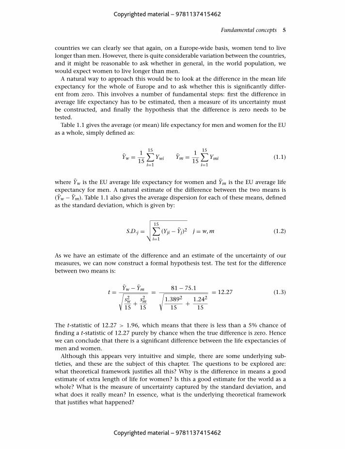
A natural way to approach this would be to look at the difference in the mean lifeexpectancy for the whole of Europe and to ask whether this is significantly differ-ent from zero. This involves a number of fundamental steps: first the difference inaverage life expectancy has to be estimated, then a measure of its uncertainty mustbe constructed, and finally the hypothesis that the difference is zero needs to betested.

Table 1.1 gives the average (or mean) life expectancy for men and women for the EUas a whole, simply defined as:

Yw = 115

15∑i=1

Ywi Ym = 115

15∑i=1

Ymi (1.1)

where Yw is the EU average life expectancy for women and Ym is the EU average lifeexpectancy for men. A natural estimate of the difference between the two means is(Yw − Ym). Table 1.1 also gives the average dispersion for each of these means, definedas the standard deviation, which is given by:

S.D.j =√√√√ 15∑

i=1

(Yji − Yj)2 j = w, m (1.2)

As we have an estimate of the difference and an estimate of the uncertainty of ourmeasures, we can now construct a formal hypothesis test. The test for the differencebetween two means is:

t = Yw − Ym√s2w

15+ s2

m15

= 81 − 75.1√1.3892

15+ 1.242

15

= 12.27 (1.3)

The t-statistic of 12.27 > 1.96, which means that there is less than a 5% chance offinding a t-statistic of 12.27 purely by chance when the true difference is zero. Hencewe can conclude that there is a significant difference between the life expectancies ofmen and women.

Although this appears very intuitive and simple, there are some underlying sub-tleties, and these are the subject of this chapter. The questions to be explored are:what theoretical framework justifies all this? Why is the difference in means a goodestimate of extra length of life for women? Is this a good estimate for the world as awhole? What is the measure of uncertainty captured by the standard deviation, andwhat does it really mean? In essence, what is the underlying theoretical frameworkthat justifies what happened?




A statistical framework

The statistical framework that underlies the approach above rests on a number of keyconcepts, the first of which is the population. We assume that there is a population ofevents or entities that we are interested in. This population is assumed to be infinitelylarge and comprises all the outcomes that concern us. The data in Table 1.1 are for theEU15 countries for the year 2002. If we were interested only in this one year for thisone set of countries, then there would be no statistical question to be asked. Accordingto the data, women lived longer than men in that year in that area. That is simply afact. But the population is much larger; it comprises all men and women in all periods,and to make an inference about this population we need some statistical framework.It might, for example, just be chance that women lived longer than men in that oneyear. How can we determine this?

The next important concepts are random variables and the population distribution.A random variable is simply a measurement of any event that occurs in an uncertainway. So, for example, the age at which a person dies is uncertain, and therefore theage of an individual at death is a random variable. Once a person dies, the age atdeath ceases to be a random variable and simply becomes an observation or a num-ber. The population distribution defines the probability of a certain event happening;for example, it is the population distribution that would define the probability of aman dying before he is 60 (Pr(Ym < 60)). The population distribution has variousmoments that define its shape. The first two moments are the mean (sometimes calledthe expected value, E(Ym) = μYm , or the average) and the variance (E(Ym−μYm )2, whichis the square of the standard deviation and is often defined as σ2

Ym).

The moments described above are sometimes referred to as the unconditionalmoments; that is to say, they apply to the whole population distribution. But we canalso condition the distribution and the moments on a particular piece of information.To make this clear, consider the life expectancy of a man living in the UK. Table 1.1tells us that this is 75 years. What, then, is the life expectancy of a man living in theUK who is already 80? Clearly not 75! An unconditional moment is the moment forthe complete distribution under consideration; a conditional moment is the momentfor those members of the population who fulfil some condition, in this case being 80.We can consider a conditional mean E(Ym|Yim = 80), in this case the mean of menaged 80, or conditional higher moments such as the conditional variance, which willbe the subject of a later chapter. This is another way of thinking of subgroups of thepopulation; we could think of the population as consisting of all people, or we couldthink of the distribution of the population of men and women separately. What wewould like to know about is the distribution of the population we are interested in,that is, the mean of the life expectancy of all men and all women. If we could mea-sure this, again there would be no statistical issue to address; we would simply knowwhether, on average, women live longer than men. Unfortunately, typically we canonly ever have direct measures on a sample drawn from the population. And we haveto use this sample to draw some inference about the population.

If the sample obeys some basic properties we can proceed to construct a methodof deriving inference. The first key idea is that of random sampling: the individ-uals who make up our sample should be drawn at random from the population.The life expectancy of a man is a random variable; that is to say, the age at deathof any individual is uncertain. Once we have observed the age at death and the




observation becomes part of our sample it ceases to be a random variable. The dataset then comprises a set of individual observations, each of which has been drawnat random from the population. So our sample of ages at death for men becomesYm = (Y1m, Y2m, . . . , Ynm). The idea of random sampling has some strong implications:because any two individuals are drawn at random from the population they should beindependent of each other; that is to say, knowing the age at death of one man tellsus nothing about the age at death of the other man. Also, as both individuals havebeen drawn from the same population, they should have an identical distribution.So, based on the assumption of random sampling, we can assert that each of the obser-vations in our sample should have an independent and identical distribution; this isoften expressed as IID.

We are now in a position to begin to construct a statistical framework. We wantto make some inference about a population distribution from which only a samplehas been observed. How can we know whether the method we choose to analyse thesample is a good one or not? The answer to this question lies in another concept,called the sampling distribution. If we draw a sample from our population, let’s sup-pose we have a method for analysing that sample. It could be anything; for example,take the odd-numbered observations and sum them and divide by 20. This will giveus an estimate. If we had another sample this would give us another estimate, and ifwe kept drawing samples this would give us a whole sequence of estimates based onthis technique. We could then look at the distribution of all these estimates, and thiswould be the sampling distribution of this particular technique. Suppose the estima-tion procedure produces an estimate of the population mean which we call Ym, thenthe sampling distribution will have a mean and a variance E(Ym) and E(Ym − E(Ym))2;in essence, the sampling distribution of a particular technique tells us most of whatwe need to know about the technique. A good estimator will generally have the prop-erty of unbiasedness, which implies that its mean value is equal to the populationfeature we want to estimate. That is, E(Ym) = η, where η is the feature of the pop-ulation we wish to measure. In the case of unbiasedness, even in a small sample weexpect the estimator to get the right answer on average. A slightly weaker require-ment is consistency; here we only expect the estimator to get the answer correct ifwe have an infinitely large sample, limn→∞ E(Ym) = η. A good estimator will be eitherunbiased or consistent, but there may be more than one possible procedure whichhas this property. In this case we can choose between a number of estimators on thebasis of efficiency; this is simply given by the variance of the sampling distribution.

Suppose we have another estimation technique, which gives rise to↔Y, which is also

unbiased; then we would prefer Y to this procedure if var(Y) < var(↔Y). This simply

means that, on average, both techniques get the answer right, but the errors made bythe first technique are, on average, smaller.

Properties of the sampling distribution of the mean

In the example above, based on Table 1.1, we calculated the mean life expectancy ofmen and women. Why is this a good idea? The answer lies in the sampling distribu-tion of the mean as an estimate of the population mean. The mean of the samplingdistribution of the mean is given by:




E

(1n

n∑i=1

Yi

)= 1

n

n∑i=1

E(Yi) =1n

n∑i=1

μY = μY (1.4)

So the expected value of the mean of a sample is equal to the population mean, andhence the mean of a sample is an unbiased estimate of the mean of the populationdistribution. The mean thus fulfils our first criterion for being a good estimator. Butwhat about the variance of the mean?

var(Y) = E(Y − μY )2 = E

⎛⎝ 1

n2

n∑i=1

n∑j=1

(Yi − μY )(Yj − μY )

⎞⎠

= 1n2

⎛⎝ n∑

i=1

var(Yi) +n∑

i=1

n∑j=1,j�=i

cov(Yi, Yj)

⎞⎠ = σ2

Yn

(1.5)

So the variance of the mean around the true population mean is related to the samplesize that is used to construct the mean and the variance of the population distribution.As the sample size increases, the variance in the population shrinks, which is quiteintuitive, as a large sample gives rise to a better estimate of the population mean. Ifthe true population distribution has a smaller mean the sampling distribution willalso have a smaller mean. Again, this is very intuitive; if everyone died at exactly thesame age the population variance would be zero, and any sample we drew from thepopulation would have a mean exactly the same as the true population mean.

Hypothesis testing and the central limit theorem

It would seem that the mean fulfils our two criteria for being a good estimate of thepopulation as a whole: it is unbiased and its efficiency increases with the sample size.However, before we can begin to test a hypothesis about this mean, we need some ideaof the shape of the whole sampling distribution. Unfortunately, while we have deriveda simple expression for the mean and the variance, it is not in general possible toderive the shape of the complete sampling distribution. A hypothesis test proceeds bymaking an assumption about the truth; we call this the null hypothesis, often referredto as H0. We then set up a specific alternative hypothesis, typically called H1. The testconsists of calculating the probability that the observed value of the statistic couldhave arisen purely by chance, assuming that the null hypothesis is true. Suppose thatour null hypothesis is that the true population mean for age at death for men is 70, H0:E(Ym) = 70. Having observed a mean of 75.1, we might then test the alternative that itis greater than 70. We would do this by calculating the probability that 75.1 could arisepurely by chance when the true value of the population mean is 70. With a continuousdistribution the probability of any exact point coming up is zero, so strictly what weare calculating is the probability of drawing any value for the mean that is greater than75.1. We can then compare this probability with a predetermined value, which we callthe significance level of the test. If the probability is less than the significance level,we reject the null hypothesis in favour of the alternative. In traditional statistics the




significance level is usually set at 1%, 5% or 10%. If we were using a 5% significancelevel and we found that the probability of observing a mean greater than 75.1 was 0.01,as 0.01 < 0.05 we would reject the hypothesis that the true value of the populationmean is 70 against the alternative that it is greater than 70.

The alternative hypothesis can typically be specified in two ways, which give rise toeither a one-sided test or a two-sided test. The example above is a one-sided test, as thealternative was that the age at death was greater than 70, but we could equally havetested the possibility that the true mean was either greater or less than 70, in whichcase we would have been conducting a two-sided test. In the case of a two-sided testwe would be calculating the probability that a value either greater than 75.1 or lessthan 70 − (75.1 − 70) = 64.9 could occur by chance. Clearly this probability would behigher than in the one-sided test.

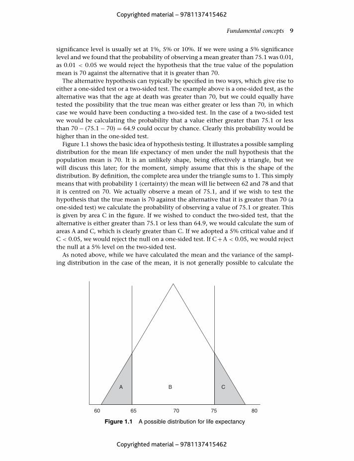
Figure 1.1 shows the basic idea of hypothesis testing. It illustrates a possible samplingdistribution for the mean life expectancy of men under the null hypothesis that thepopulation mean is 70. It is an unlikely shape, being effectively a triangle, but wewill discuss this later; for the moment, simply assume that this is the shape of thedistribution. By definition, the complete area under the triangle sums to 1. This simplymeans that with probability 1 (certainty) the mean will lie between 62 and 78 and thatit is centred on 70. We actually observe a mean of 75.1, and if we wish to test thehypothesis that the true mean is 70 against the alternative that it is greater than 70 (aone-sided test) we calculate the probability of observing a value of 75.1 or greater. Thisis given by area C in the figure. If we wished to conduct the two-sided test, that thealternative is either greater than 75.1 or less than 64.9, we would calculate the sum ofareas A and C, which is clearly greater than C. If we adopted a 5% critical value and ifC < 0.05, we would reject the null on a one-sided test. If C+A < 0.05, we would rejectthe null at a 5% level on the two-sided test.

As noted above, while we have calculated the mean and the variance of the sampl-ing distribution in the case of the mean, it is not generally possible to calculate the

60 65 70 75 80

BA C

Figure 1.1 A possible distribution for life expectancy




shape of the complete distribution. However, there is a remarkable theorem whichdoes generally allow us to do this as the sample size grows large. This is the central limittheorem.

Central limit theorem

If a set of data is IID with n observations, (Y1, Y2, . . . Yn), and with a finite variancethen as n goes to infinity the distribution of Y becomes normal. So as long as n isreasonably large we can think of the distribution of the mean as being approximatelynormal.

This is a remarkable result; what it says is that, regardless of the form of the popula-tion distribution, the sampling distribution will be normal as long as it is based on alarge enough sample. To take an extreme example, suppose we think of a lottery whichpays out one winning ticket for every 100 tickets sold. If the prize for a winning ticketis $100 and the cost of each ticket is $1, then, on average, we would expect to earn $1per ticket bought. But the population distribution would look very strange; 99 out ofevery 100 tickets would have a return of zero and one ticket would have a return of$100. If we tried to graph the distribution of returns it would have a huge spike at zeroand a small spike at $100 and no observations anywhere else. But, as long as we drawa reasonably large sample, when we calculate the mean return over the sample it willbe centred on $1 with a normal distribution around 1.

The importance of the central limit theorem is that it allows us to know what thesampling distribution of the mean should look like as long as the mean is based on areasonably large sample. So we can now replace the arbitrary triangular distribution inFigure 1.1 with a much more reasonable one, the normal distribution.

A final small piece of our statistical framework is the law of large numbers. Thissimply states that if a sample (Y1, Y2, . . . Yn) is IID with a finite variance then Y isa consistent estimator of μ, the true population mean. This can be formally stated asPr(|Y−μ| < ε) → 1 as n → ∞, meaning that the probability that the absolute differencebetween the mean estimate and the true population mean will be less than a smallpositive number tends to one as the sample size tends to infinity. This can be provedstraightforwardly, since, as we have seen, the variance of the sampling distribution ofthe mean is inversely proportional to n; hence as n goes to infinity the variance ofthe sampling distribution goes to zero and the mean is forced to the true populationmean.

We can now summarize: Y is an unbiased and consistent estimate of the true popu-lation mean μ; it is approximately distributed as a normal distribution with a variancewhich is inversely proportional to n; this may be expressed as N(μ, σ2/n). So if we sub-tract the population mean from Y and divide by its standard deviation we will create avariable which has a mean of zero and a unit variance. This is called standardizing thevariable.

Y − μ√σ2/n

∼ N(0, 1) (1.6)




One small problem with this formula, however, is that it involves σ2. This is thepopulation variance, which is unknown, and we need to derive an estimate of it. Wemay estimate the population variance by:

S2 = 1n − 1

n∑i=1

(Yi − Y)2 (1.7)

Here we divide by n−1 because we effectively lose one observation when we estimatethe mean. Consider what happens when we have a sample of one. The estimate of themean would be identical to the one observation, and if we divided by n = 1 we wouldestimate a variance of zero. By dividing by n − 1 the variance is undefined for a sampleof one. Why is S2 a good estimate of the population variance? The answer is that it isessentially simply another average; hence the law of large numbers applies and it willbe a consistent estimate of the true population variance.

Now we are finally in a position to construct a formal hypothesis test. The basic testis known as the student ‘t’ test and is given by:

t = Y − μ√S2/n

(1.8)

When the sample is small this will follow a student t-distribution, which can be lookedup in any standard set of statistical tables. In practice, however, once the sample islarger than 30 or 40, the t-distribution is almost identical to the standard normaldistribution, and in econometrics it is common practice simply to use the normaldistribution. The value of the normal distribution that implies 0.025 in each tail ofthe distribution is 1.96. This is the critical value that goes with a two-tailed test at a5% significance level. So if we want to test the hypothesis that our estimate of the lifeexpectancy of men of 75.1 actually is a random draw from a population with a meanof 70, then the test would be:

t = 75.1 − 70√S2/3.87

= 5.1.355

= 14.37

This is greater than the 5% significance level of 1.96, and so we would reject thenull hypothesis that the true population mean is 70. Equivalently, we could evaluatethe proportion of the distribution that is associated with an absolute t-value greaterthan 4.1, which would then be the probability value discussed above. Formally theprobability or p-value is given by:

p-value = PrH0 (|Y − μ| > |Yact − μ|) = PrH0 (|t| > |tact |)

So if the t-value is exactly 1.96 the p-value will be 0.05, and when the t-value isgreater than 1.96 the p-value will be less than 0.05. They contain exactly the sameinformation, simply expressed in a different way. The p-value is useful in other cir-cumstances, however, as it can be calculated for a range of different distributionsand can avoid the need to consult statistical tables, as its interpretation is alwaysstraightforward.




69.3 70 70.71 75.1

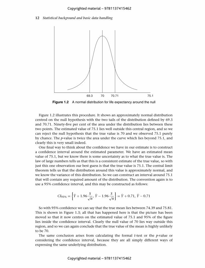
Figure 1.2 A normal distribution for life expectancy around the null

Figure 1.2 illustrates this procedure. It shows an approximately normal distributioncentred on the null hypothesis with the two tails of the distribution defined by 69.3and 70.71. Ninety-five per cent of the area under the distribution lies between thesetwo points. The estimated value of 75.1 lies well outside this central region, and so wecan reject the null hypothesis that the true value is 70 and we observed 75.1 purelyby chance. The p-value is twice the area under the curve which lies beyond 75.1, andclearly this is very small indeed.

One final way to think about the confidence we have in our estimate is to constructa confidence interval around the estimated parameter. We have an estimated meanvalue of 75.1, but we know there is some uncertainty as to what the true value is. Thelaw of large numbers tells us that this is a consistent estimate of the true value, so withjust this one observation our best guess is that the true value is 75.1. The central limittheorem tells us that the distribution around this value is approximately normal, andwe know the variance of this distribution. So we can construct an interval around 75.1that will contain any required amount of the distribution. The convention again is touse a 95% confidence interval, and this may be constructed as follows:

CI95% ={

Y + 1.96S√n

, Y − 1.96S√n

}= Y + 0.71, Y − 0.71

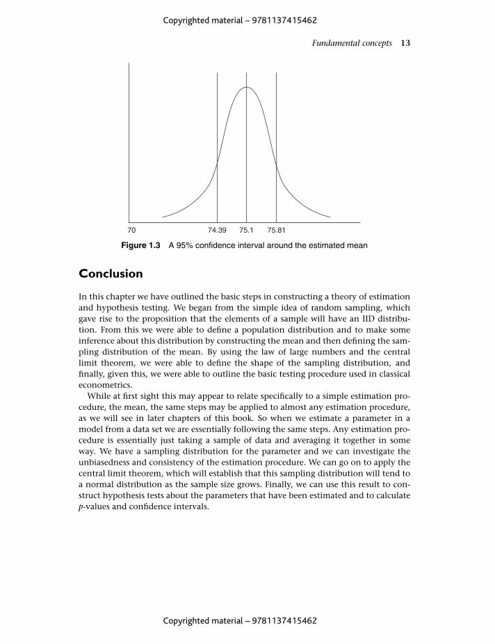
So with 95% confidence we can say that the true mean lies between 74.39 and 75.81.This is shown in Figure 1.3; all that has happened here is that the picture has beenmoved so that it now centres on the estimated value of 75.1 and 95% of the figurelies inside the confidence interval. Clearly the null value of 70 lies way outside thisregion, and so we can again conclude that the true value of the mean is highly unlikelyto be 70.

The same conclusion arises from calculating the formal t-test or the p-value orconsidering the confidence interval, because they are all simply different ways ofexpressing the same underlying distribution.




74.3970 75.1 75.81

Figure 1.3 A 95% confidence interval around the estimated mean

Conclusion

In this chapter we have outlined the basic steps in constructing a theory of estimationand hypothesis testing. We began from the simple idea of random sampling, whichgave rise to the proposition that the elements of a sample will have an IID distribu-tion. From this we were able to define a population distribution and to make someinference about this distribution by constructing the mean and then defining the sam-pling distribution of the mean. By using the law of large numbers and the centrallimit theorem, we were able to define the shape of the sampling distribution, andfinally, given this, we were able to outline the basic testing procedure used in classicaleconometrics.

While at first sight this may appear to relate specifically to a simple estimation pro-cedure, the mean, the same steps may be applied to almost any estimation procedure,as we will see in later chapters of this book. So when we estimate a parameter in amodel from a data set we are essentially following the same steps. Any estimation pro-cedure is essentially just taking a sample of data and averaging it together in someway. We have a sampling distribution for the parameter and we can investigate theunbiasedness and consistency of the estimation procedure. We can go on to apply thecentral limit theorem, which will establish that this sampling distribution will tend toa normal distribution as the sample size grows. Finally, we can use this result to con-struct hypothesis tests about the parameters that have been estimated and to calculatep-values and confidence intervals.



Index

Adaptive expectations model, 236,239–241

Adjusted R2, defined, 72–73Akaike information criterion, defined, 73

ADF tests and, 357, 360, 363, 364ARIMA modelling and, 288

Almon lag procedure, 233, 235–236AR(1), see First-order autoregressive process

(AR(1)), pth-order autoregressiveprocess ARCH effects and ARCHmodels

ARCH models, general approach, 299–308computer example, 302–306mathematical approach, 306–309

ARCH tests for heteroskedasticity, 146–148computer example, 147–148steps for, 147

ARIMA models, defined, 275computer example, 289–294estimating and forecasting with, 288

Augmented Dickey–Fuller test (ADF),general, 357cointegration equation and, 376–377computer example, 362–365steps for, 359–360

Autocorrelation, defined, 157ARCH tests and, 146causes of, 157computer examples, 162, 167, 169, 172,

175, 177consequences of ignoring, 159–161detecting, graphical method, 162detecting, tests for, 164–173first-order, 158higher-order, 158lagged dependent variable and, 171–172residual plot and, 162resolving, 174–178

Autoregressive (AR) Models, 277–281Auxiliary regressions, 108–109

heteroskedasticity and, 126–137LM test approach and, 126–137

Bar graph, 18Base year, defined, 21–22Best linear unbiased estimators

in multiple regression, 70–72in simple regression, 38–40

Box–Cox transformation, 189–201computer example, l99–201

Breusch–Godfrey test, 168–170computer example, 169

Breusch–Pagan test, 125–128computer example, 127–128

CAPM, 87–97advanced Eviews programming, 96–97Eviews commands, 93–96Eviews programming, 90–93steps in the application, 89–90

Causality, defined, 336computer example, 338–341Granger causality test, 336–338Sims causality test, 338testing for, 334–335

Central limit theorem, 8–10Chi-square test, defined, 80Chow test, defined, 227–228Cobb–Douglas production function, 23,

51–52double log model and, 188–189

Cochrane–Orcutt iterative procedure,175–176

vs Hildreth–Lu search procedure, 176Coefficients

correlation, 109drivers, 428–429dummy, 216–219first-order autocorrelation, 158testing linear restrictions of, 75–77testing the significance of the OLS, 46–47

Cointegration, defined, 368computer example, 392–399and the ECM, general approach, 371and the ECM, mathematical approach,

372

513



514 Index

Cointegration, defined – continuedEngle and Granger approach, 380–390Johansen approach, 368–375mathematical approach, 372–376in panel data, 473–478testing for, 376–379, 387–391

Conditional variance, 98–289Confidence interval, 12–14, 45–46Consistency of OLS estimators,

in simple regression, 42–43in multiple regression, 70

Constant returns to scale, 75–76Constant term

dummy variables and, 211Consumer price index, 21Consumption income relationship, 52Correlation

first-order serial, see AutocorrelationCorrelogram

for ARIMA models, 277, 278, 282, 285in Eviews, 289–290

Cross-sectional datadefined, 15in Eviews, 48in Stata, 494

Day-of-the-week effect, 229–232Data, 14–16

base period and, 21–22basic handling, 17–21cross-sectional, 15entering in EViews, 488–489entering in Stata, 493–497panel, 16–17time series, 15–16

Diagnostic checking in ARIMA modelling,286, 288

Dickey-Fuller tests, 355–357computer example, 362–365performing in EViews, 359performing in Stata, 361

Differencing, 23generalized differencing approach, 173in spurious regressions, 351

Distributed lag models, 232–236Almon transformation and, 235–236Koyck transformation and, 233–235

Double-log model, 188–189Dummy variables, defined, 210

Chow test, 227–228day-of-the-week effect, 229–232dependent variables, 244–261effect of, 210–215multiple categories, 222–224seasonal, 221–222slope shift using, 216–217structural change testing, 225–228trap, 219–220trap and exact multicollinearity, 106

Durbin h-test, 170–172

Durbin–Watson testfor serial correlation, 164–167

Dynamic modelsin panel data, 458in time series data, 232–241

Efficiency of the OLS coefficients, 40–41E-GARCH model, 317–318

computer example, 318Equation

reduced form, 245–246simultaneous, 244–253

Error(s)correction model, see Error-correctionmodel, measurementnormality of, 194specification, 181

Error-correction model, defined, 371cointegration and, 370computer example, 392–399

Estimationwith ARIMA models, 288of simultaneous equation models,

248–249OLS method, 32–35time-varying coefficient method,

426–428using dummy variables, 215–222

Estimator(s)best linear unbiased, 38–40, 69–72consistency, 42–43, 70efficiency, 40unbiasedness, 39–40, 70

EViews software, basics, 486–490Exact identification, 246Exact multicollinearity, 104–106Excel and OLS estimation, 53–55

F-form of the likelihood ratio test, 77Finite prediction error, 73First-order autocorrelation coefficient, 158First-order autoregressive process (AR(1)),

defined, 277miscellaneous derivations with, 277–278

Fitted straight line, 31–33Fixed effects model, 444–445F-test for overall significance, 78–79Function(s)

autocorrelation, 281–284Cobb–Douglas production, 23, 51, 76–77

impulse response, 417Functional forms, 185–189

double-log, 188–189including interaction terms, 187linear-log, 185–186logarithmic, 180log-linear, 188polynomial, 186–187reciprocal, 186



Index 515

GARCH models, defined, 399advanced Eviews programming, 322–326application, 326–329computer examples, 302–326in Stata, 320–321

Generalized least squares, 148–149General to specific approach, 203–204Glesjer test, 128–130

computer example in EViews, 129computer example in Stata, 129–130

GMM estimators, 459Goldfeld–Quandt test, 133–135

computer example, 134–135Goodness of fit, defined, 43–44

in limited dependent variable model,260–261

measurement of, 43–44Granger causality test, 336–338

application, 338–341computer example, 343–344steps for, 336–338

Hendry/LSE approach, 203–204Heteroskedasticity

computer examples, 137–149consequences of, 120–122defined, 117illustration of, 117–118resolving, 149–153testing for, 124–135

Heteroskedasticity consistent estimationmethod, 150

Hildreth–Lu search procedure, 175–176vs Cochrane–Orcutt research procedure,

175Histogram, 18–20

and normality tests, 194–195Homoskedasticity, 36, 118, 298Hypothesis testing

and the central limit theorem, 8–10confidence intervals and, 45–46p-value approach, 47rule of thumb, 46–47steps to, 46testing individual coefficients, 75testing linear restrictions, 75testing the significance of OLS

coefficients, 46

Identification problem, defined, 245–246,287

cointegrated systems and, 406–411computer example, 250–253, 410–411conditions for, 246example of, 247–248order condition and, 405rank condition and, 406

Im, Pesaran and Shin panel unit-root test,470

Imperfect multicollinearity, 106–107Impulse response functions, 417

Indirect least squares, 248Instrumental variables, 426, 456Integrated of order d, 285, 351Integrated of order one, 350–351Integration

Dickey–Fuller tests of, 342–344Phillips–Perron tests of, 344–346testing for the order of, 342

Intercept termdummy variables and, 210–212, 214–215

Invertibility in MA models, 283

January effect application, 224–225Joint significance, 78–79

Kao panel cointegration test, 473Keynesian model, 53–57Koyck lag model, 233–235

Lagged dependent variablesadaptive expectations model and,

239–241partial adjustment model and, 236–237serial correlation and, 170

Lagrange multiplier (LM) test, 81–82for heteroskedasticity, 125–133in EViews, 82for serial correlation, 167–168for testing linear restrictions, 75–76

Larsson et al. panel cointegration test,477–478

Least squares method, defined, 32derivation of solutions for the multiple

model, 64–66derivation of solutions for the simple

model, 32–35derivation of solutions with matrix

algebra, 66–67Levin and Lin panel unit-root test, 469–470Likelihood ratio test, 77

F-form of, 77–78Limited dependent variable regression,

254–271Linear-log model, 185–186Linear probability model, 255

problems with, 256–257Ljung–Box test statistic, 288Logit model, 258

computer example, 267–270general approach, 258–259goodness of fit and, 260interpretation of estimates, 259–260mathematical approach, 261–262in Stata, 270

Log-linear model, 188Log-log model, 188–189Long-run behaviour, error-correction

model and, 370



516 Index

Maddala and Wu panel unit-root test, 471Marginal effect

of functional forms, 185–189interpretation of, 185, 189

Marginal propensity to consume, 52, 187,213, 241

McCoskey and Kao panel cointegrationtest, 475

Mean group estimator, 461–462Misspecification, 31, 37, 77, 181–204

tests for, 193–197RESET test, 195

Model(s)adaptive expectations, 239–241ARCH, 297–327ARIMA, 275–295autoregressive, 236-241, 277–282distributed lag, 232–236double-log, 188–189dynamic, 232, 458E-GARCH, 318error correction, 370–374fixed effects, 444–445GARCH, 309–311GARCH-M, 312Hendry/LSE approach, 203–204Keynesian, 53Koyck, 233–235with lagged dependent variables, 171,

236–238linear-log, 185–186linear panel data, 417linear probability model, 245Logit, 258–263log-linear, 188log-log, 188–189multinomial Logit, 265–266multinomial Probit, 265–266partial adjustment, 236–237polynomial, 186–187Probit, 263–264random effect, 445–446reciprocal, 186solving, 414–423TGARCH, 317–318Tobit, 267VAR, 333–336

Modellingaverage economic regression, 202–203general to specific, 202–203Hendry/LSE approach, 203–204simple to general, 194traditional view, 202–203

Moving average models, 282–285Multicollinearity

computer examples, 110–115consequences of, 105–106, 107–109defined, 104detecting, 109–110

exact, 106–107imperfect, 106–107perfect, 104–106

Multinomial Logit model, 266Multinomial Probit model, 266Multiple regression computer examples,

82–84defined, 64in Eviews, 74goodness of fit and, 72hypothesis testing and, 75–82in Stata, 74

Non-nested models, tests for, 197–199Nonstationarity, defined, 348

and spurious regression, 351and unit roots, 355–358

OLS, see Ordinary least squaresOmitted variables, 84–85

LM tests for, 84Bias, 182and the plug-in solution, 183–184

Order condition, 246, 405Ordinary Least Squares, defined, 32

GLS procedure and, 149heteroskedasticity and consequences,

120–124serial correlation and consequences,

159–162Overidentification, defined, 248Overparametrized model, 286

Panel data, defined, 16–17advantages of, 442common constant, 443cointegration and, 473–478different methods of estimation, 443dynamic, 458estimating in Eviews, 451estimating in Stata, 456fixed effects, 444–445Hausman test, 446heterogeneous, 434inserting in EViews, 447–450inserting in Stata, 453–456linear model, 443random effects, 445–446unit root tests, 468–473

Park test, 142Partial adjustment model, 236–237

computer example, 237–239Partial autocorrelation function, 282, 288,

295Pedroni panel cointegration test, 476–477Perfect multicollinearity, 106–107Pooled mean group estimator, 462–464Pooling assumption, 442, 460



Index 517

Probit model, 263–264computer example, 267–271general approach, 263mathematical approach, 264

Production function, 51pth-order autoregressive process (AR(p)),

279–280pth-order serial correlation, 158–159p-value approach, 47

Qualitative information, defined, 210dummy variables and, 210–214with multiple categories, 222slope term and, 212–213with multiple categories, 218–220

R2, 44problems with, 44–45

R2 adjusted for degrees of freedom, 72Random effects model, 445–446Rank condition, 246, 406Reciprocal functional form, 186Redundant variables, 79–84, 182–183Regression

Dickey–Fuller, 355–357Multiple, 64–96Simple, 29–58spurious, 348sum of squares, 43–44

Regressions specification error test (RESET),195–197

Residual, defined, 21test of normality, 193

Robust inference, 123, 162

Scatter plots, 18, 31detecting autocorrelation, 162–164detecting heteroskedasticity, 124–126in Eviews, 18simple regression, 31spurious regressions, 352–353in Stata, 19

Seasonal dummies, 221–222application, 224–225

Serial correlation, see AutocorrelationSignificantly different from zero, 5, 47Simple linear regression model, 30

computer examples, 53–57interpretation of coefficients, 50

Simple to general modelling, 202–203Simultaneous equation model, 244

consequences of ignoring simultaneity,244

estimation of, 248–250identification problem, 245structure of reduced forms, 245–246

Specification error, defined, 181, 195

Spurious correlation, 348–350Spurious regression, 348–350Stata software, basics, 491–499Stationarity, defined, 277Stationary time series, 277Structural breaks, 17, 18, 287Structural change, 226

Test(ing)For ARCH effects, 301for autocorrelation, 162–174for causality, 336–338for cointegration, Engle–Grangerapproach, 376–379for cointegration, Johansen approach,

379–387of goodness of fit, 73, 260for heteroskedasticity, 124–133hypothesis, 8–10, 45–47individual coefficients, 46, 75for the joint significance of the Xs,

78–79linear restrictions, 75–77for misspecification, 193–199for structural change, 228–229

Time-varying coefficient models, 425–438choosing coefficient drivers, 429–433coefficient drivers, 428–429estimation, 426–428

Time series data, 15–16Time series models, see ARIMA modelsTotal sum of squares, 43–44t test, 47, 80–81TVC models, see Time-varying coefficient

models

Unbiasedness of OLS coefficientsmultiple regression, 70simple regression, 39–40

Unit roots, defined, 348–353in Eviews, 359Dickey–Fuller test and, 355–357panel data and, 442–445Phillips–Perron test, 357–359in Stata, 361

VAR models, see Vector autoregressivemodels

Variable(s)dummy, 210instrumental, 426, 430, 459lagged dependent, 171–172omitted, 181–182qualitative, 210redundant, 182–183

Variationexplained, 44total, 44unexplained, 44



518 Index

Vector autoregressive (VAR) models,334–336

pros and cons, 335–336in Eviews, 341–344in Stata, 344

Wald test, defined, 77computer example, 82–84

performing in EViews, 80Weighted least squares, 148–150White’s heteroskedasticity consisted

estimation, 150White’s test, 135–137, 144

computer example, 144in Eviews, 136in Stata, 137



9781137415462 01 prexxvii · PDF file · 2015-08-14Consequences of autocorrelation for the OLS estimators 159 A general approach 159 A more mathematical approach 160 Detecting...

Documents