9.7 and 9.10 Taylor Polynomials and Taylor Series.

9.7 and 9.10Taylor Polynomials and

Taylor Series

Suppose we wanted to find a fourth degree polynomial of the form:

2 3 40 1 2 3 4P x a a x a x a x a x

ln 1f x x at 0x that approximates the behavior of

If we make f (0) = P(0), f ’(0) = P’(0), f ’’(0) = P’’(0), and so on, then we would have a pretty good approximation.

2 3 40 1 2 3 4P x a a x a x a x a x ln 1f x x

ln 1f x x

0 ln 1 0f

2 3 40 1 2 3 4P x a a x a x a x a x

00P a 0 0a

1

1f x

x

10 1

1f

2 31 2 3 42 3 4P x a a x a x a x

10P a 1 1a

2

1

1f x

x

10 1

1f

22 3 42 6 12P x a a x a x

20 2P a 2

1

2a

3

12

1f x

x

0 2f

3 46 24P x a a x

30 6P a 3

2

6a

4

4

16

1f x

x

4 0 6f

4424P x a

440 24P a 4

6

24a

2 3 41 2 60 1

2 6 24P x x x x x

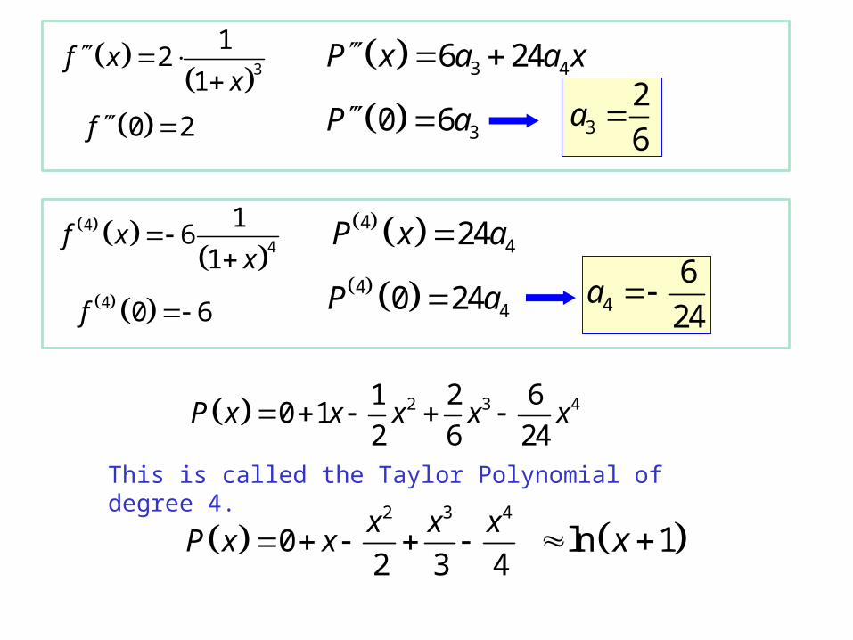
This is called the Taylor Polynomial of degree 4.

ln 1x 2 3 4

02 3 4

x x xP x x

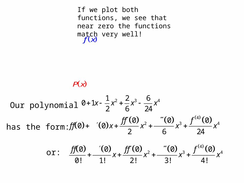
Our polynomial 2 3 41 2 6

0 12 6 24

x x x x

has the form: 42 3 40 0 0

0 02 6 24

f f ff f x x x x

or: 42 3 40 0 0 0 0

0! 1! 2! 3! 4!

f f f f fx x x x

P x

f x

If we plot both functions, we see that near zero the functions match very well!

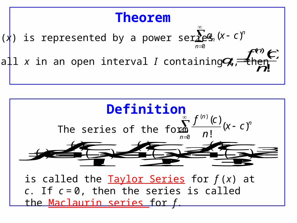
Definition

The series of the form

2 3

1! 2! 3!

f c f c f cf c x c x c x c

Theorem

If f (x) is represented by a power series

for all x in an open interval I containing c, then( ) ( )

!

n

n

f ca

n

is called the Taylor Series for f (x) at c. If c = 0, then the series is called the Maclaurin series for f .

0

( )nn

n

a x c

( )

0

( )( )

!

nn

n

f cx c

n

cosf x x 0 1f

sinf x x 0 0f

cosf x x 0 1f

sinf x x 0 0f

4 cosf x x 4 0 1f

2 4 6 8 10

cos 1 2! 4! 6! 8! 10!

x x x x xx

2 3 4cos2! 3!

1 0

4!

11 0x x x x x

Example

( ) cosf x xFind the Maclaurin series for

( ) cos 2f x x

Rather than start from scratch, we can use the function that we already know:

2 4 6 8 102 2 2 2 2

cos 2 1 2! 4! 6! 8! 10!

x x x x xx

Example

Find the Maclaurin series for

2 4 6 8 10

cos 1 2! 4! 6! 8! 10!

x x x x xx

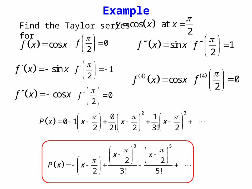
cos at 2

y x x

2 3

0 10 1

2 2! 2 3! 2P x x x x

cosf x x 02

f

sinf x x 12

f

cosf x x 02

f

sinf x x 12

f

4 cosf x x 4 02

f

3 5

2 2

2 3! 5!

x xP x x

ExampleFind the Taylor series for

sin x

cos x

sin x

cos x

sin x

0

1

0

1

0

0nf nf x

2 3 4sin2

0 1 00 1

! 3! 4!x x x x x

3 5 7

sin 3! 5! 7!

x x xx x

Example

Find the Maclaurin series for ( ) sinf x x

2 30 00 0

2! 3!

f fP x f f x x x

1( )

1f x

x

11 x

21 x

32 1 x

46 1 x

524 1 x

1

1

2

6 3!

24 4!

0nf nf x

2 3 42 31

1 2! 3!

! 4!1

!1

4x x x x

x

2 3 411

1x x x x

x

This is a geometric series witha = 1 and r = x.

Example

Find the Maclaurin series for

2 30 00 0

2! 3!

f fP x f f x x x

( ) ln 1f x x

ln 1 x

11 x

21 x

32 1 x

46 1 x

0

1

1

2

6 3!

0nf nf x

2 3 4ln 12

1

! 3! 4

20 1

!

3!x x x x x

2 3 4

ln 12 3 4

x x xx x

Example

Find the Maclaurin series for

2 30 00 0

2! 3!

f fP x f f x x x

( ) xf x e

xe

xe

xe

xe

xe

1

1

1

1

1

0nf nf x

2 3 41 1 11 1

2! 3! 4!xe x x x x

2 3 4

12! 3! 4!

x x x xe x

Example

Find the Maclaurin series for

2 3 4

12! 3! 4!

x x x xe x

An amazing use for infinite series:

Substitute xi for x.

2 3 4 5 6

1 2! 3! 4! 5! 6!

xi xi xi xi xi xie xi

2 2 3 3 4 4 5 5 6 6

1 2! 3! 4! 5! 6!

xi x i x i x i x i x ie xi

2 3 4 5 6

1 2! 3! 4! 5! 6!

xi x x i x x i xe xi

2 4 6 3 5

1 2! 4! 6! 3! 5!

xi x x x x xe i x

Factor out the i terms.

Euler’s Formula

2 4 6 3 5

1 2! 4! 6! 3! 5!

xi x x x x xe i x

This is the series for cosine.

This is the series for sine.

cos sinxie ix x Let x

cos sinie i

1 0ie i

1 0ie This amazing identity contains the five most famous numbers in mathematics, and shows that they are interrelated.

Taylor series are used to estimate the value of functions (at least theoretically - nowadays we can usually use the calculator or computer to calculate directly.)

An estimate is only useful if we have an idea of how accurate the estimate is.

When we use part of a Taylor series to estimate the value of a function, the end of the series that we do not use is called the remainder. If we know the size of the remainder, then we know how close our estimate is.

Ex: Use to approximate over .2 4 61 x x x 2

1

1 x 1,1

the truncation error is , which is .8 10 12 x x x 8

21

x

x

When you “truncate” a number, you drop off the end.

Taylor’s Theorem with Remainder

If f has derivatives of all orders in an open interval I containing a, then for each positive integer n and for each x

in I:

2

2! !

nn

n

f fa af f f Rx a a x a x a x a xn

Lagrange Form of the Remainder

11

1 !

nn

n

f cR x x a

n

Remainder after partial sum Sn

where c is between

a and x.

This is also called the remainder of order n or the error term.

This is called Taylor’s Inequality.

Taylor’s Inequality

Lagrange Form of the Remainder

11

1 !

nn

n

f cR x x a

n

If M is the maximum value of on the interval

between a and x, then:

1nf x

1

1 !n

n

MR x x a

n

Note that this looks just

like the next term in the

series, but “a” has been

replaced by the number

“c” in . 1nf c

Find the Lagrange Error Bound when is used

to approximate and .

2

2

xx

ln 1 x 0.1x ln 1f x x 1

1f x x

21f x x

32 1f x x

22

0 00

1 2!

f ff f x x Rx x

Remainder after 2nd order term

2

202

xf x Rx x

On the interval , decreases, so

its maximum value occurs at the left end-point.

.1,.1 3

2

1 x

3

2

1 .1M

3

2

.9 2.74348422497

32.7435 .1

3!nR x 0.000457

Lagrange Error Bound

x ln 1 x2

2

xx error

.1 .0953102 .095 .000310

.1 .1053605 .105 .000361