91.204.201 Computing IV Chapter Three: imgproc module Image Processing Part I Xinwen Fu.

91.204.201 Computing IV

Chapter Three: imgproc moduleImage Processing

Part I

Xinwen Fu

CS@UML

References Application Development in Visual Studio Reading assignment: Chapter 3

An online OpenCV Quick Guide with nice examples

By Dr. Xinwen Fu 2

CS@UML

Outline 3.1 Smoothing Images

3.2 Eroding and Dilating

3.3 More Morphology Transformations

3.4 Image Pyramids

3.5 Basic Thresholding Operations

3.6 Making your own linear filters!

3.7 Adding borders to your images

By Dr. Xinwen Fu 3

3.8 Sobel Derivatives

3.9 Laplace Operator

3.10 Canny Edge Detector

3.11 Hough Line Transform

3.13 Hough Circle Transform

3.14 Remapping

CS@UML

Smoothing Smoothing, also called blurring, is a simple

and frequently used image processing operation.

There are many reasons for smoothing. Reduce noise

Other uses later

By Dr. Xinwen Fu 4

CS@UML

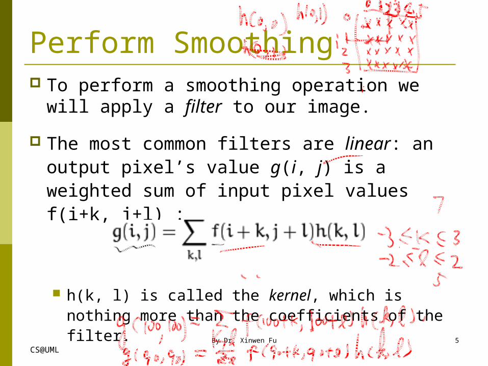
Perform Smoothing To perform a smoothing operation we will

apply a filter to our image.

The most common filters are linear: an output pixel’s value g(i, j) is a weighted sum of input pixel values f(i+k, j+l) :

h(k, l) is called the kernel, which is nothing more than the coefficients of the filter.

By Dr. Xinwen Fu 5

CS@UML

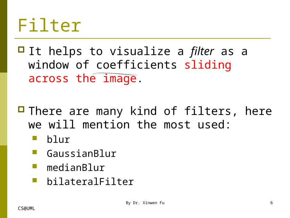
Filter It helps to visualize a filter as a window of

coefficients sliding across the image.

There are many kind of filters, here we will mention the most used: blur GaussianBlur medianBlur bilateralFilter

By Dr. Xinwen Fu 6

CS@UML

Normalized Box Filter This filter is the simplest of all! Each

output pixel is the mean of its kernel neighbors All of them contribute with equal weights

The kernel is below:

By Dr. Xinwen Fu 7

CS@UML

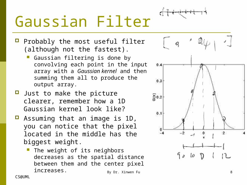
Gaussian Filter Probably the most useful filter

(although not the fastest). Gaussian filtering is done by

convolving each point in the input array with a Gaussian kernel and then summing them all to produce the output array.

Just to make the picture clearer, remember how a 1D Gaussian kernel look like?

Assuming that an image is 1D, you can notice that the pixel located in the middle has the biggest weight. The weight of its neighbors decreases

as the spatial distance between them and the center pixel increases.

By Dr. Xinwen Fu 8

CS@UML

2D Gaussian Remember that a 2D Gaussian can be

represented as :

where µ is the mean (the peak) and σ represents the variance (per each of the variables x and y)

By Dr. Xinwen Fu 9

CS@UML

Median Filter The median filter run through each

element of the signal (in this case the image) and replace each pixel with the median of its neighboring pixels (located in a square neighborhood around the evaluated pixel).

By Dr. Xinwen Fu 10

CS@UML

Bilateral Filter Sometimes the filters do not only dissolve the

noise, but also smooth away the edges. To avoid this (at certain extent at least), use a bilateral

filter. The bilateral filter also considers the neighboring

pixels with weights assigned to each of them. These weights have two components, the first of which

is the same weighting used by the Gaussian filter. The second component takes into account the difference

in intensity between the neighboring pixels and the evaluated one.

For a more detailed explanation you can check this link

By Dr. Xinwen Fu 11

CS@UML

Bilateral filtering function

Where

One example - Shift-invariant Gaussian filtering

Domain filter where

Range filter where

Bilateral Filter - Gaussian Case

By Dr. Xinwen Fu 12

CS@UML

Example Code Loads an image

Applies 4 different kinds of filters (explained in Theory) and show the filtered images sequentially

By Dr. Xinwen Fu 13

CS@UML




3.4 Image Pyramids




By Dr. Xinwen Fu 14






3.14 Remapping

CS@UML

Morphological Operations A set of operations based on shapes.

Morphological operations apply a structuring element to an input image and generate an output image.

Two basic morphological operations: Erosion and Dilation. Removing noise Isolation of individual elements and joining

disparate elements in an image. Finding of intensity bumps or holes in an image

By Dr. Xinwen Fu 15

CS@UML

Dilation

By Dr. Xinwen Fu 16

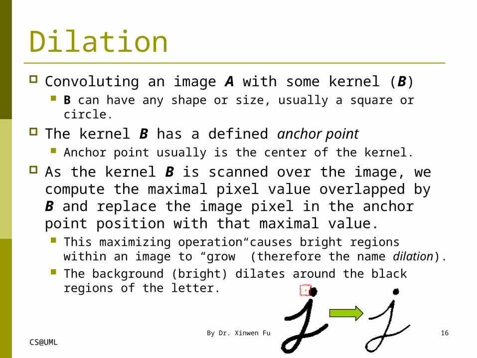
Convoluting an image A with some kernel (B) B can have any shape or size, usually a square or circle.

The kernel B has a defined anchor point Anchor point usually is the center of the kernel.

As the kernel B is scanned over the image, we compute the maximal pixel value overlapped by B and replace the image pixel in the anchor point position with that maximal value. This maximizing operation causes bright regions within

an image to “grow” (therefore the name dilation). The background (bright) dilates around the black regions

of the letter.

CS@UML

Erosion Compute a local minimum over the area of

the kernel B. As the kernel B is scanned over the image, we

compute the minimal pixel value overlapped by B and replace the image pixel under the anchor point with that minimal value.

In the result below, the bright areas of the image (the background, apparently), get thinner, whereas the dark zones (the “writing”) gets bigger.

By Dr. Xinwen Fu 17

CS@UML

Example Code Load an image (can be RGB or grayscale) Create two windows (one for dilation output, the

other for erosion) Create a set of 2 Trackbars for each operation:

The first trackbar “Element” returns either erosion_elem or dilation_elem

The second trackbar “Kernel size” return erosion_size or dilation_size for the corresponding operation.

Every time we move any slider, the user’s function Erosion or Dilation will be called and it will update the output image based on the current trackbar values.

By Dr. Xinwen Fu 18

CS@UML




3.4 Image Pyramids




By Dr. Xinwen Fu 19






3.14 Remapping

CS@UML

Opening Obtained by erosion of an image followed by

dilation. Useful for removing small objects (it is assumed

that the objects are bright on a dark foreground)

For example, the image at the left is the original and the image at the right is the result after applying the opening transformation. We can observe that the small spaces in the corners of

the letter tend to disappear.

By Dr. Xinwen Fu 20

CS@UML

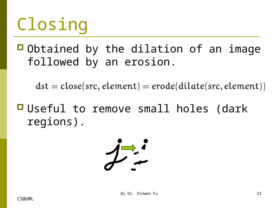
Closing Obtained by the dilation of an image

followed by an erosion.

Useful to remove small holes (dark regions).

By Dr. Xinwen Fu 21

CS@UML

Morphological Gradient It is the difference between the dilation

and the erosion of an image.

It is useful for finding the outline of an object as can be seen below:

By Dr. Xinwen Fu 22

CS@UML

Top Hat It is the difference between an input image

and its opening.

By Dr. Xinwen Fu 23

CS@UML

Black Hat It is the difference between the closing

and its input image

By Dr. Xinwen Fu 24

CS@UML

Example Code Load an image Create a window to display results of the

Morphological operations Create 3 Trackbars for the user to enter

parameters of morphology operation

By Dr. Xinwen Fu 25

CS@UML




3.4 Image Pyramids




By Dr. Xinwen Fu 26






3.14 Remapping

CS@UML

Theory Two possible options of converting an

image to a size different than its original: Upsize the image (zoom in) or Downsize it (zoom out).

We analyze first the use of Image Pyramids, which are widely applied in a huge range of vision applications.

By Dr. Xinwen Fu 27

CS@UML

Image Pyramid An image pyramid is a collection of images - all

arising from a single original image - that are successively downsampled until some desired stopping point is reached.

There are two common kinds of image pyramids: Gaussian pyramid: Used to downsample images Laplacian pyramid: Used to reconstruct an upsampled

image from an image lower in the pyramid (with less resolution)

We’ll use the Gaussian pyramid.

By Dr. Xinwen Fu 28

CS@UML

Gaussian Pyramid Imagine the pyramid as a set of layers

The higher the layer, the smaller the size.

Every layer is numbered from bottom to top, so layer (i+1) (denoted as Gi+1) is smaller than layer i (Gi).

By Dr. Xinwen Fu 29

CS@UML

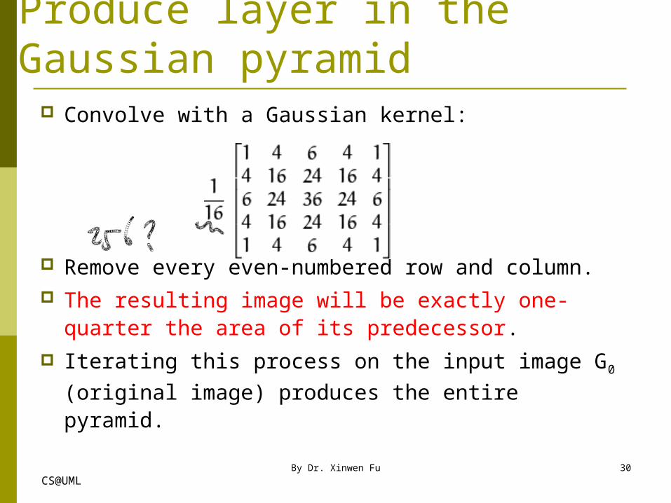
Produce layer in the Gaussian pyramid

Convolve with a Gaussian kernel:

Remove every even-numbered row and column. The resulting image will be exactly one-quarter

the area of its predecessor. Iterating this process on the input image G0

(original image) produces the entire pyramid.

By Dr. Xinwen Fu 30

CS@UML

Upsample The procedure above was useful to downsample an

image. What if we want to make it bigger?

First, upsize the image to twice the original in each dimension, wit the new even rows and columns filled with zeros (0)

Perform a convolution with the same kernel shown above (multiplied by 4) to approximate the values of the “missing pixels”

These two procedures (downsampling and upsampling as explained above) are implemented by the OpenCV functions pyrUp and pyrDown

By Dr. Xinwen Fu 31

CS@UML

Example Code

By Dr. Xinwen Fu 32

CS@UML




3.4 Image Pyramids




By Dr. Xinwen Fu 33






3.14 Remapping

CS@UML

What is Thresholding? Simplest segmentation method

Example: Separate out regions of an image corresponding to objects which we want to analyze.

This separation is based on the variation of intensity between the object pixels and the background pixels.

To differentiate the pixels we are interested in from the rest (which will eventually be rejected), we perform a comparison of each pixel intensity value with respect to a threshold (determined according to the problem to solve).

Once we have separated properly the important pixels, we can set them with a determined value to identify them (i.e. we can assign them a value of 0 (black), 255 (white) or any value that suits your needs).

By Dr. Xinwen Fu 34

CS@UML

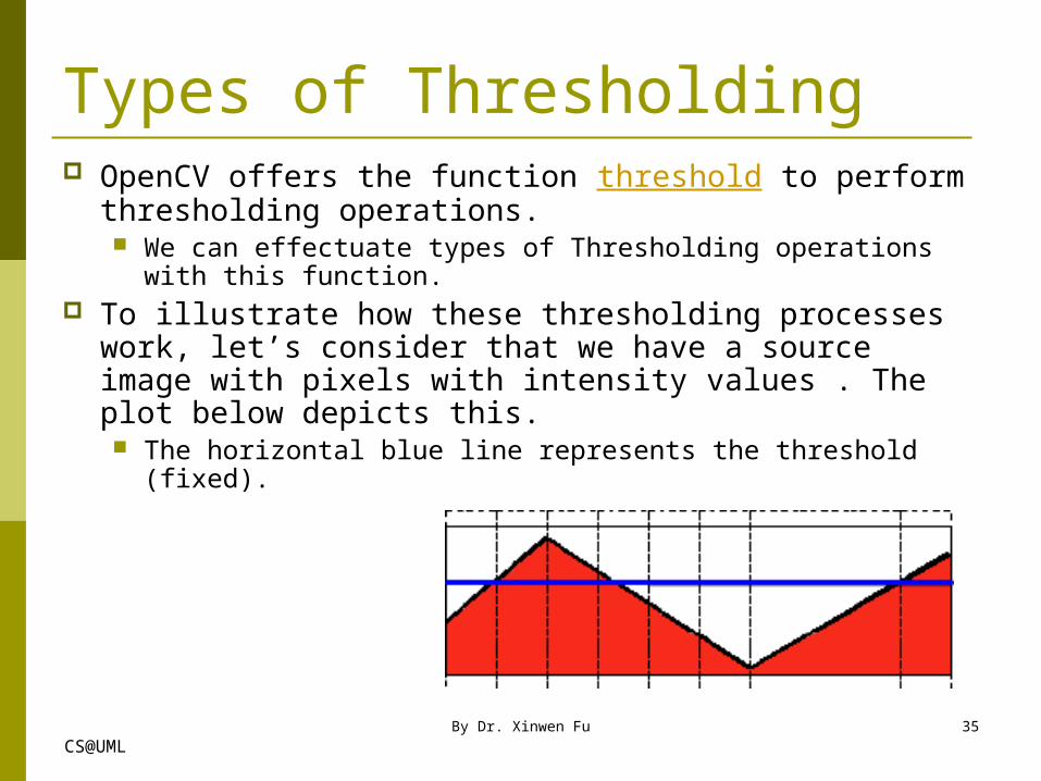
Types of Thresholding OpenCV offers the function threshold to perform

thresholding operations. We can effectuate types of Thresholding operations with

this function. To illustrate how these thresholding processes work,

let’s consider that we have a source image with pixels with intensity values . The plot below depicts this. The horizontal blue line represents the threshold (fixed).

By Dr. Xinwen Fu 35

CS@UML

Threshold Binary This thresholding operation can be expressed as:

So, if the intensity of the pixel src(x, y) is higher than thresh, then the new pixel intensity is set to a maxVal. Otherwise, the pixels are set to 0.

By Dr. Xinwen Fu 36

CS@UML

Threshold Binary, Inverted This thresholding operation can be

expressed as:

If the intensity of the pixel is higher than , then the new pixel intensity is set to a 0. Otherwise, it is set to maxVal.

By Dr. Xinwen Fu 37

CS@UML

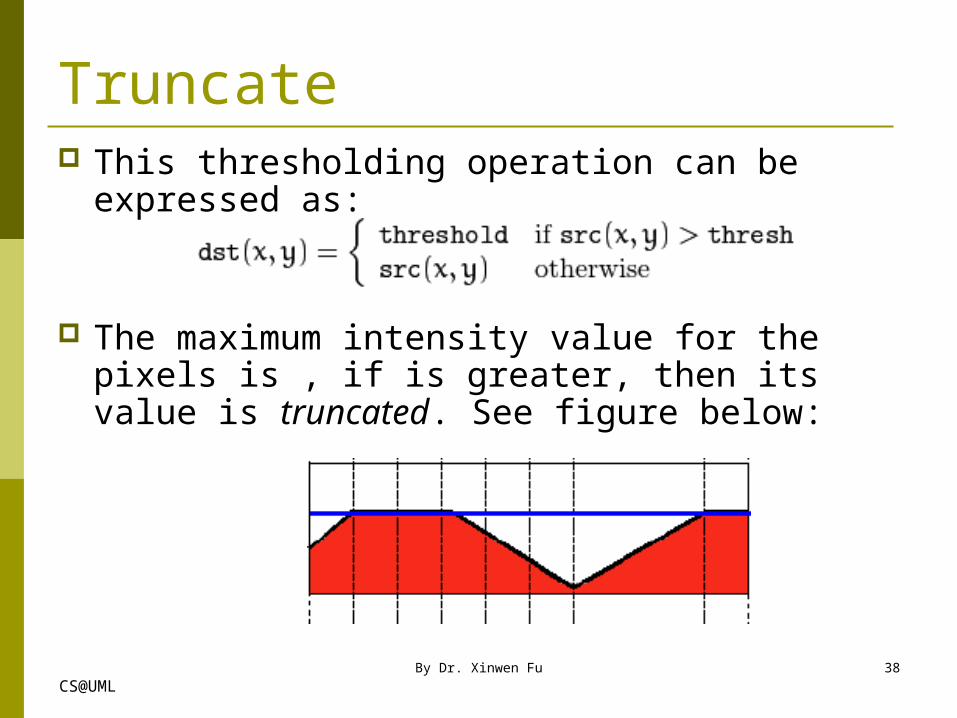
Truncate This thresholding operation can be expressed

as:

The maximum intensity value for the pixels is , if is greater, then its value is truncated. See figure below:

By Dr. Xinwen Fu 38

CS@UML

Threshold to Zero This operation can be expressed as:

If src(x,y) is lower than thresh, the new pixel value will be set to .

By Dr. Xinwen Fu 39

CS@UML

Threshold to Zero, Inverted This operation can be expressed as:

If src(x, y) is greater than thresh, the new pixel value will be set to 0.

By Dr. Xinwen Fu 40

CS@UML

Example Code

By Dr. Xinwen Fu 41

CS@UML




3.4 Image Pyramids




By Dr. Xinwen Fu 42






3.14 Remapping

CS@UML

Convolution In a very general sense, convolution is an

operation between every part of an image and an operator (kernel).

A kernel is essentially a fixed size array of numerical coefficients along with an anchor point in that array, which is typically located at the center.

By Dr. Xinwen Fu 43

CS@UML

How does convolution with a kernel work? Assume you want to know the resulting value of a

particular location in the image. The value of the convolution is calculated in the following way:1. Place the kernel anchor on top of a determined pixel,

with the rest of the kernel overlaying the corresponding local pixels in the image.

2. Multiply the kernel coefficients by the corresponding image pixel values and sum the result.

3. Place the result to the location of the anchor in the input image.

4. Repeat the process for all pixels by scanning the kernel over the entire image.

By Dr. Xinwen Fu 44

CS@UML

Equation of Convolution Expressing the procedure above in the

form of an equation we would have:

Fortunately, OpenCV provides you with the function filter2D so you do not have to code all these operations.

By Dr. Xinwen Fu 45

CS@UML

Example Code Loads an image Performs a normalized box

filter. For instance, for a kernel of size size =3, the kernel would be:

The program will perform the filter operation with kernels of sizes 3, 5, 7, 9 and 11.

The filter output (with each kernel) will be shown during 500 milliseconds

By Dr. Xinwen Fu 46

CS@UML




3.4 Image Pyramids




By Dr. Xinwen Fu 47






3.14 Remapping

CS@UML

Theory In our previous tutorial we learned to use

convolution to operate on images.

how to handle the boundaries? How can we convolve them if the evaluated points are at

the edge of the image?

What most of OpenCV functions do is to copy a given image onto another slightly larger image and then automatically pads the boundary This way, the convolution can be performed over the

needed pixels without problems (the extra padding is cut after the operation is done).

By Dr. Xinwen Fu 48

CS@UML

OpenCV Making Borders We will briefly explore two ways of

defining extra padding (border) for an image: BORDER_CONSTANT: Pad the image with a

constant value (i.e. black or 0)

BORDER_REPLICATE: The row or column at the very edge of the original is replicated to the extra border.

By Dr. Xinwen Fu 49

CS@UML

Example Code Load an image Let the user choose what kind of padding use in

the input image. There are two options: Constant value border: Applies a padding of a constant

value for the whole border. This value will be updated randomly each 0.5 seconds.

Replicated border: The border will be replicated from the pixel values at the edges of the original image.

The user chooses either option by pressing ‘c’ (constant) or ‘r’ (replicate)

The program finishes when the user presses ‘ESC’

By Dr. Xinwen Fu 50

CS@UML




3.4 Image Pyramids




By Dr. Xinwen Fu 51






3.14 Remapping

CS@UML

Theory1. One of the most important

convolutions is the computation of derivatives in an image (or an approximation to them).

detect the edges present in the image. For instance:

2. In an edge, the pixel intensity changes in a notorious way

A good way to express changes is by using derivatives.

A high change in gradient indicates a major change in the image

By Dr. Xinwen Fu 52

CS@UML

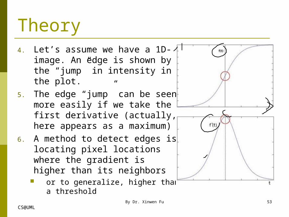
Theory4. Let’s assume we have a 1D-

image. An edge is shown by the “jump” in intensity in the plot.

5. The edge “jump” can be seen more easily if we take the first derivative (actually, here appears as a maximum)

6. A method to detect edges is locating pixel locations where the gradient is higher than its neighbors

or to generalize, higher than a threshold

By Dr. Xinwen Fu 53

CS@UML

Sobel Operator The Sobel Operator is a discrete

differentiation operator. It computes an approximation of the gradient of an image intensity function.

The Sobel Operator combines Gaussian smoothing and differentiation.

By Dr. Xinwen Fu 54

CS@UML

Formulation - We calculate two derivatives: Horizontal changes:

This is computed by convolving with a kernel with odd size. For example for a kernel size of 3, would be computed as:

Vertical changes: This is computed by convolving with a kernel with odd size. For example for a kernel size of 3, would be computed as:

By Dr. Xinwen Fu 55

CS@UML

Formulation - We calculate two derivatives: At each point of the

image we calculate an approximation of the gradient in that point by combining both results above:

Although sometimes the following simpler equation is used:

By Dr. Xinwen Fu 56

CS@UML

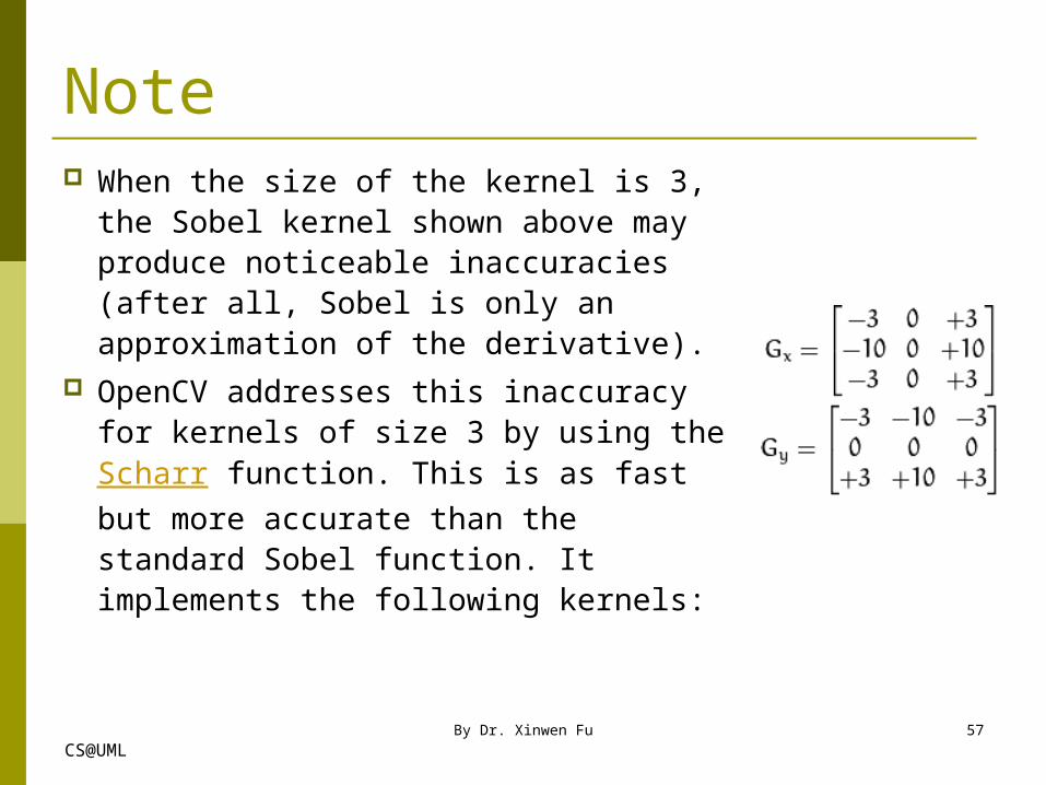
Note When the size of the kernel is 3, the

Sobel kernel shown above may produce noticeable inaccuracies (after all, Sobel is only an approximation of the derivative).

OpenCV addresses this inaccuracy for kernels of size 3 by using the Scharr function. This is as fast but more accurate than the standard Sobel function. It implements the following kernels:

By Dr. Xinwen Fu 57

CS@UML

Example Code Applies the Sobel Operator and generates as output

an image with the detected edges bright on a darker background.

You can check out more information of this function in the OpenCV reference (Scharr). Also, in the sample code, you will notice that above the code for Sobel function there is also code for the Scharr function commented. Uncommenting it (and obviously commenting the Sobel stuff) should give you an idea of how this function works.

By Dr. Xinwen Fu 58

CS@UML




3.4 Image Pyramids




By Dr. Xinwen Fu 59






3.14 Remapping

CS@UML

Theory Sobel Operator as based on the fact that in the edge

area, the pixel intensity shows a “jump” or a high variation of intensity.

Getting the first derivative of the intensity, we observed that an edge is characterized by a maximum, as it can be seen in the figure:

By Dr. Xinwen Fu 60

CS@UML

And...what happens if we take the second derivative? The second derivative is zero! So, we can also use this

criterion to attempt to detect edges in an image. However, note that zeros will not only appear in edges

(they can appear in other meaningless locations); This can be solved by applying filtering where needed.

By Dr. Xinwen Fu 61

CS@UML

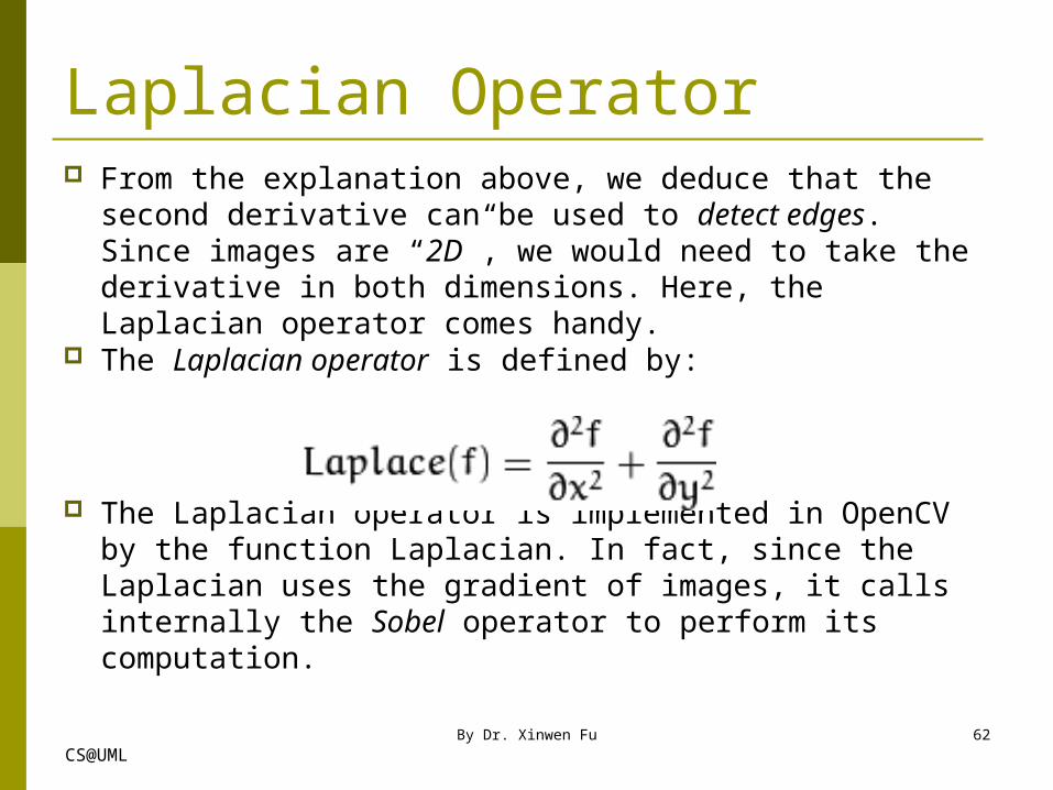
Laplacian Operator From the explanation above, we deduce that the

second derivative can be used to detect edges. Since images are “2D”, we would need to take the derivative in both dimensions. Here, the Laplacian operator comes handy.

The Laplacian operator is defined by:

The Laplacian operator is implemented in OpenCV by the function Laplacian. In fact, since the Laplacian uses the gradient of images, it calls internally the Sobel operator to perform its computation.

By Dr. Xinwen Fu 62

CS@UML

Example Code Loads an image Remove noise by applying a Gaussian blur

and then convert the original image to grayscale

Applies a Laplacian operator to the grayscale image and stores the output image

Display the result in a window

By Dr. Xinwen Fu 63

CS@UML




3.4 Image Pyramids




By Dr. Xinwen Fu 64






3.14 Remapping

CS@UML

Theory The Canny Edge detector was developed by

John F. Canny in 1986. Also known to many as the optimal detector, Canny algorithm aims to satisfy three main criteria: Low error rate: Meaning a good detection of only

existent edges. Good localization: The distance between edge

pixels detected and real edge pixels have to be minimized.

Minimal response: Only one detector response per edge.

By Dr. Xinwen Fu 65

CS@UML

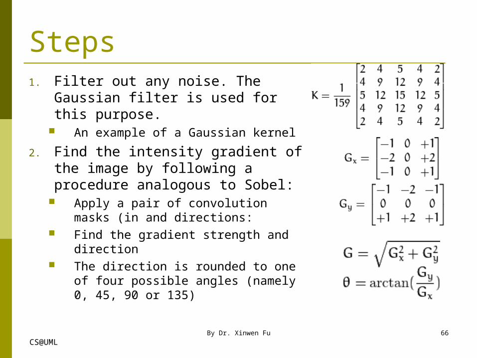
Steps1. Filter out any noise. The Gaussian

filter is used for this purpose. An example of a Gaussian kernel

2. Find the intensity gradient of the image by following a procedure analogous to Sobel:

Apply a pair of convolution masks (in and directions:

Find the gradient strength and direction

The direction is rounded to one of four possible angles (namely 0, 45, 90 or 135)

By Dr. Xinwen Fu 66

CS@UML

Steps (Cont’d) Non-maximum suppression is applied.

This removes pixels that are not considered to be part of an edge and only thin lines (candidate edges) will remain.

Hysteresis: The final step. Canny does use two thresholds (upper and lower): If a pixel gradient is higher than the upper threshold, the

pixel is accepted as an edge If a pixel gradient value is below the lower threshold, then

it is rejected. If the pixel gradient is between the two thresholds, then it

will be accepted only if it is connected to a pixel that is above the upper threshold.

Canny recommended a upper:lower ratio between 2:1 and 3:1.

By Dr. Xinwen Fu 67

CS@UML

Example Code Asks the user to enter a numerical value to

set the lower threshold for our Canny Edge Detector (by means of a Trackbar)

Applies the Canny Detector and generates a mask (bright lines representing the edges on a black background).

Applies the mask obtained on the original image and display it in a window.

By Dr. Xinwen Fu 68

CS@UML




3.4 Image Pyramids




By Dr. Xinwen Fu 69






3.14 Remapping

CS@UML

Hough Line Transform The Hough Line Transform is a transform

used to detect straight lines.

To apply the Transform, first an edge detection pre-processing is desirable.

By Dr. Xinwen Fu 70

CS@UML

How does it work?1. A line in the image space

can be expressed with two variables. In the Cartesian coordinate

system: Parameters: (m, b). In the Polar coordinate

system: Parameters: (r, θ) For Hough Transforms, we will

express lines in the Polar system. Hence, a line equation can be written as:

Arranging the terms: r= xcosθ + ysinθ

By Dr. Xinwen Fu 71

CS@UML

How does it work? (Cont’d)2. For each point (x0, y0), the

family of lines that goes through it is defined as: Meaning that each pair (rθ, θ)

represents each line that passes by (x0, y0).

3. For a given (x0, y0), we plot the family of lines that goes through it, and we get a sinusoid. For instance, for x0 =8 and y0 =6

we get the following plot (in a plane – θ, r)

We consider only points such that r > 0 and 0 < θ < 2ϖ.

By Dr. Xinwen Fu 72

CS@UML

How does it work? (Cont’d)4. Do the same operation

above for all the points in an image. If the curves of two different points intersect in the plane θ - r , that means that both points belong to a same line.

For instance, following with the example above and drawing the plot for two more points: x1=9, y1=4 and x2=12, y2=3, we get left figure:

The three plots intersect in one single point (0.925, 9.6), these coordinates are the parameters (θ, r) or the line in which (x0 =8, y0 =6), (x1=9, y1=4) and (x2=12, y2=3) lay.By Dr. Xinwen Fu 73

CS@UML

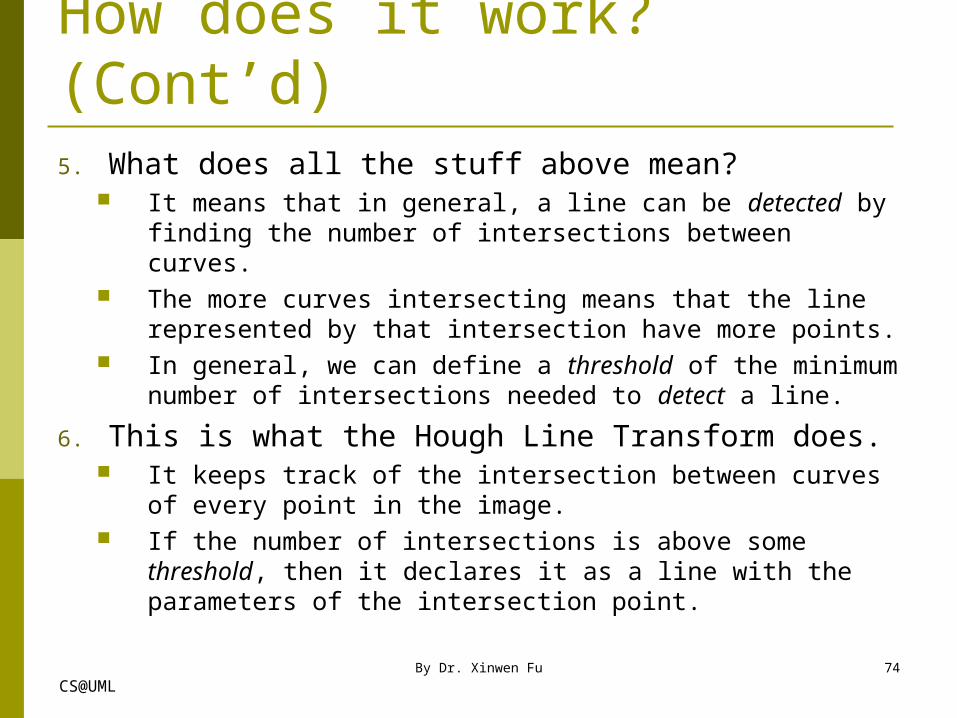
How does it work? (Cont’d)5. What does all the stuff above mean?

It means that in general, a line can be detected by finding the number of intersections between curves.

The more curves intersecting means that the line represented by that intersection have more points.

In general, we can define a threshold of the minimum number of intersections needed to detect a line.

6. This is what the Hough Line Transform does. It keeps track of the intersection between curves of

every point in the image. If the number of intersections is above some threshold,

then it declares it as a line with the parameters of the intersection point.

By Dr. Xinwen Fu 74

CS@UML

Standard and Probabilistic Hough Line Transform The Standard Hough Transform

It consists in pretty much what we just explained in the previous section. It gives you as result a vector of couples

In OpenCV it is implemented with the function HoughLines

The Probabilistic Hough Line Transform A more efficient implementation of the Hough Line

Transform. It gives as output the extremes of the detected lines

In OpenCV it is implemented with the function HoughLinesP

By Dr. Xinwen Fu 75

CS@UML

Example Code Loads an image Applies either a Standard Hough Line

Transform or a Probabilistic Line Transform.

Display the original image and the detected line in two windows.

By Dr. Xinwen Fu 76

CS@UML




3.4 Image Pyramids




By Dr. Xinwen Fu 77






3.14 Remapping

CS@UML

Hough Circle Transform Hough Circle Transform works in

a roughly analogous way to the Hough Line Transform explained in the previous tutorial.

In the line detection case, a line was defined by two parameters (r, θ) .

In the circle case, we need three parameters to define a circle: where (xcenter, ycenter) define the

center position (green point) and r is the radius, which allows us to completely define a circle

By Dr. Xinwen Fu 78

CS@UML

Hough gradient method For sake of efficiency, OpenCV implements

a detection method slightly trickier than the standard Hough Transform: The Hough gradient method.

For more details, please check the book Learning OpenCV or your favorite Computer Vision bibliography

By Dr. Xinwen Fu 79

CS@UML

Example Code Loads an image and blur it to reduce the

noise Applies the Hough Circle Transform to the

blurred image . Display the detected circle in a window.

By Dr. Xinwen Fu 80

CS@UML




3.4 Image Pyramids




By Dr. Xinwen Fu 81






3.14 Remapping

CS@UML

What is remapping Taking pixel from one place in the image and

locate them in another position in a new image. To accomplish the mapping process, it might be

necessary to do some interpolation for non-integer pixel locations, since there will not always be a one-to-one-pixel correspondence between source and destination images.

We can express the remap for every pixel (x, y) location as: where g() is remapped image, f() the source image and

h(x, y) is the mapping function that operates on (x, y).

By Dr. Xinwen Fu 82

CS@UML

remap Let’s think in a quick example.

Imagine that we have an image and, say, we want to do a remap such that:

What would happen? It is easily seen that the image would flip in the direction.

E.g, consider the input image: observe how the red circle changes

positions with respect to x (considering x the horizontal direction):

In OpenCV, the function remap offers a simple remapping implementation.

By Dr. Xinwen Fu 83

CS@UML

Example Code Loads an image Each second, apply 1 of 4 different

remapping processes to the image and display them indefinitely in a window.

Wait for the user to exit the program

By Dr. Xinwen Fu 84

CS@UMLBy Dr. Xinwen Fu 85

91.204.201 Computing IV Chapter Three: imgproc module Image Processing Part I Xinwen Fu.

Documents

uml filter

uml gaussian filter

uml median filter

uml bilateral filter

useful filter

xinwen fu6 slide

xinwen fu2 slide

xinwen fu9 slide