Introduction Insertion Sort Selection Sort Bubble Sort Quick Sort Merge Sort Lower Bound Count Sort Conclusion 9. Sorting Frank Stephan March 20, 2014

Welcome message from author
This document is posted to help you gain knowledge. Please leave a comment to let me know what you think about it! Share it to your friends and learn new things together.
Transcript

Introduction Insertion Sort Selection Sort Bubble Sort Quick Sort Merge Sort Lower Bound Count Sort Conclusion
9. Sorting
Frank Stephan
March 20, 2014

Introduction Insertion Sort Selection Sort Bubble Sort Quick Sort Merge Sort Lower Bound Count Sort Conclusion
Introduction
Sorting
Given a list (ai , . . . , an) of n elements output a permutation(a′i , . . . , a
′n) such that a′i ≤ a′j whenever i ≤ j .
Many Algorithms!
Insertion sort, selection sort, bubble sort, quick sort, count sort,bucket sort, etc.

Introduction Insertion Sort Selection Sort Bubble Sort Quick Sort Merge Sort Lower Bound Count Sort Conclusion
Introduction
AlgoRythmics
http://www.youtube.com/user/AlgoRythmics
Introduction Insertion Sort Selection Sort Bubble Sort Quick Sort Merge Sort Lower Bound Count Sort Conclusion
Insertion Sort
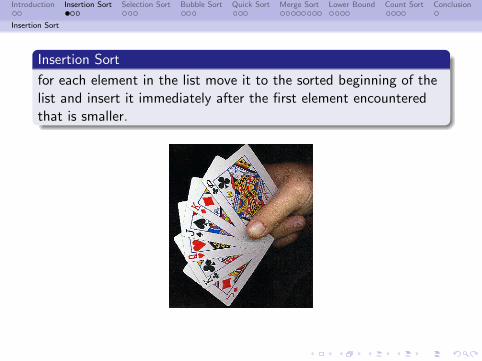
Insertion Sort
for each element in the list move it to the sorted beginning of thelist and insert it immediately after the first element encounteredthat is smaller.
Introduction Insertion Sort Selection Sort Bubble Sort Quick Sort Merge Sort Lower Bound Count Sort Conclusion
Insertion Sort
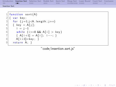
1 f u n c t i o n s o r t (A)2 va r key ;3 f o r ( j =1; j<A. l e n g t h ; j++)4 key = A[ j ] ;5 i = j−16 wh i l e ( i>=0 && A[ i ] > key )7 A[ i +1] = A[ i ] ; i −−; 8 A[ i +1]=key ; 9 r e t u r n A ;
”code/insertion sort.js”
Introduction Insertion Sort Selection Sort Bubble Sort Quick Sort Merge Sort Lower Bound Count Sort Conclusion
Insertion Sort
Insertion Sort
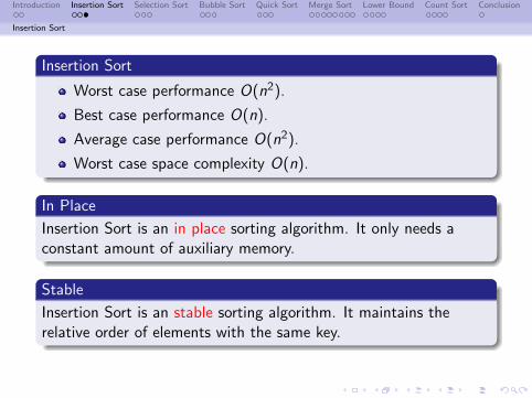
Worst case performance O(n2).
Best case performance O(n).
Average case performance O(n2).
Worst case space complexity O(n).
In Place
Insertion Sort is an in place sorting algorithm. It only needs aconstant amount of auxiliary memory.
Stable
Insertion Sort is an stable sorting algorithm. It maintains therelative order of elements with the same key.
Introduction Insertion Sort Selection Sort Bubble Sort Quick Sort Merge Sort Lower Bound Count Sort Conclusion
Selection Sort
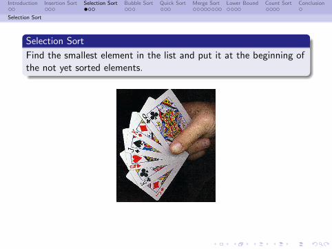
Selection Sort
Find the smallest element in the list and put it at the beginning ofthe not yet sorted elements.

Introduction Insertion Sort Selection Sort Bubble Sort Quick Sort Merge Sort Lower Bound Count Sort Conclusion
Selection Sort
1 f u n c t i o n s o r t (A)2 va r i , j , key , tmp ;3 f o r ( i =0; i<A. l e n g t h ; i++)4 key = i ;5 f o r ( j= i +1; j < A. l e n g t h ; j++)6 i f (A [ j ] < A[ key ] ) key=j ; 7 tmp=A[ key ] ; A [ key ] = A[ i ] ; A [ i ] = tmp ; 8 r e t u r n A ;
”code/selection sort.js”
Introduction Insertion Sort Selection Sort Bubble Sort Quick Sort Merge Sort Lower Bound Count Sort Conclusion
Selection Sort
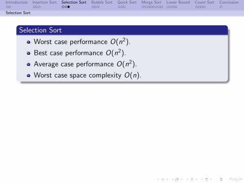
Selection Sort
Worst case performance O(n2).
Best case performance O(n2).
Average case performance O(n2).
Worst case space complexity O(n).

Introduction Insertion Sort Selection Sort Bubble Sort Quick Sort Merge Sort Lower Bound Count Sort Conclusion
Bubble Sort
Bubble Sort
Move up the largest elements in the list.
Introduction Insertion Sort Selection Sort Bubble Sort Quick Sort Merge Sort Lower Bound Count Sort Conclusion
Bubble Sort
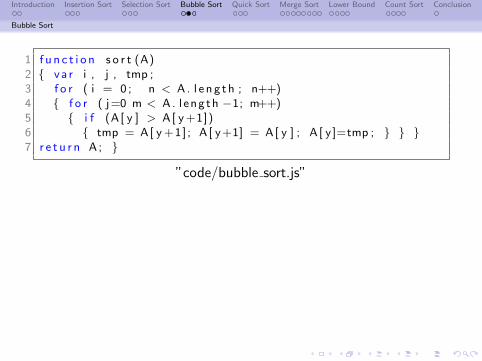
1 f u n c t i o n s o r t (A)2 va r i , j , tmp ;3 f o r ( i = 0 ; n < A. l e n g t h ; n++)4 f o r ( j=0 m < A. l eng th −1; m++)5 i f (A [ y ] > A[ y+1])6 tmp = A[ y+1] ; A [ y+1] = A[ y ] ; A [ y ]=tmp ; 7 r e t u r n A ;
”code/bubble sort.js”
Introduction Insertion Sort Selection Sort Bubble Sort Quick Sort Merge Sort Lower Bound Count Sort Conclusion
Bubble Sort
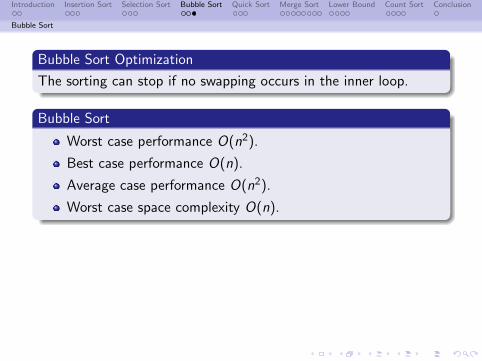
Bubble Sort Optimization
The sorting can stop if no swapping occurs in the inner loop.
Bubble Sort
Worst case performance O(n2).
Best case performance O(n).
Average case performance O(n2).
Worst case space complexity O(n).
Introduction Insertion Sort Selection Sort Bubble Sort Quick Sort Merge Sort Lower Bound Count Sort Conclusion
Quick Sort
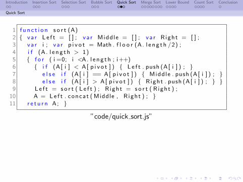
Quick Sort
Choose an element in the list. Let us call it the pivot. Move allelements smaller than the pivot element at the beginning of thelist. Repeat the operation for both the list before the pivot and thelist after the pivot.
Introduction Insertion Sort Selection Sort Bubble Sort Quick Sort Merge Sort Lower Bound Count Sort Conclusion
Quick Sort
1 f u n c t i o n s o r t (A)2 va r L e f t = [ ] ; va r Middle = [ ] ; va r R ight = [ ] ;3 va r i ; v a r p i v o t = Math . f l o o r (A . l e n g t h /2) ;4 i f (A . l e n g t h > 1)5 f o r ( i =0; i <A. l e n g t h ; i++)6 i f (A [ i ] < A[ p i v o t ] ) L e f t . push (A[ i ] ) ; 7 e l s e i f (A [ i ] == A[ p i v o t ] ) Middle . push (A[ i ] ) ; 8 e l s e i f (A [ i ] > A[ p i v o t ] ) Right . push (A[ i ] ) ; 9 L e f t = s o r t ( L e f t ) ; R ight = s o r t ( R ight ) ;
10 A = Le f t . concat ( Middle , R ight ) ; 11 r e t u r n A ;
”code/quick sort.js”
Introduction Insertion Sort Selection Sort Bubble Sort Quick Sort Merge Sort Lower Bound Count Sort Conclusion
Quick Sort
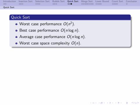
Quick Sort
Worst case performance O(n2).
Best case performance O(n log n).
Average case performance O(n log n).
Worst case space complexity O(n).
Introduction Insertion Sort Selection Sort Bubble Sort Quick Sort Merge Sort Lower Bound Count Sort Conclusion
Merge Sort
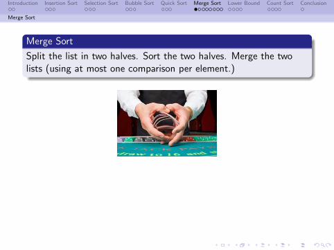
Merge Sort
Split the list in two halves. Sort the two halves. Merge the twolists (using at most one comparison per element.)

Introduction Insertion Sort Selection Sort Bubble Sort Quick Sort Merge Sort Lower Bound Count Sort Conclusion
Merge Sort
Merge Sort
1 f u n c t i o n s o r t (A)2 va r r e s u l t ;3 i f (A . l e n g t h >1)4 va r p i v o t = Math . f l o o r (A . l e n g t h / 2) ;5 va r L e f t = A. s l i c e (0 , p i v o t ) ;6 va r R ight = A. s l i c e ( p i vo t , A . l e n g t h ) ;7 L e f t = s o r t ( L e f t ) ; R ight = s o r t ( R ight ) ;8 r e s u l t = merge ( Le f t , R ight ) ; 9 e l s e r e s u l t = A;
10 r e t u r n r e s u l t ;
”code/merge sort.js”
Introduction Insertion Sort Selection Sort Bubble Sort Quick Sort Merge Sort Lower Bound Count Sort Conclusion
Merge Sort
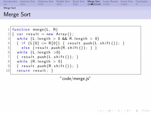
Merge Sort
1 f u n c t i o n merge (L , R)2 va r r e s u l t = new Array ( ) ;3 wh i l e (L . l e n g t h > 0 && R. l e n g t h > 0)4 i f ( L [ 0 ] <= R [ 0 ] ) r e s u l t . push (L . s h i f t ( ) ) ; 5 e l s e r e s u l t . push (R . s h i f t ( ) ) ; 6 wh i l e (L . l e n g t h >0)7 r e s u l t . push (L . s h i f t ( ) ) ; 8 wh i l e (R . l e n g t h > 0)9 r e s u l t . push (R . s h i f t ( ) ) ;
10 r e t u r n r e s u l t ;
”code/merge.js”

Introduction Insertion Sort Selection Sort Bubble Sort Quick Sort Merge Sort Lower Bound Count Sort Conclusion
Merge Sort
Recurrence Relation
The number of comparisons is T (n) defined by the followingrecurrence relation (equation).
If n ≤ 2 then T (n) = 1
else T (n) = 2 · T (n
2) + n
How to solve a recurrence equation?
Introduction Insertion Sort Selection Sort Bubble Sort Quick Sort Merge Sort Lower Bound Count Sort Conclusion
Merge Sort
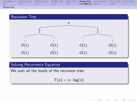
Recursion Tree
n
n2
· · ·
O(1)
O(1)
· · ·
O(1)
O(1)
n2
· · ·
O(1)
O(1)
· · ·
O(1)
O(1)
Solving Recurrence Equation
We sum all the levels of the recursion tree.
T (n) = n · log(n)
Introduction Insertion Sort Selection Sort Bubble Sort Quick Sort Merge Sort Lower Bound Count Sort Conclusion
Merge Sort
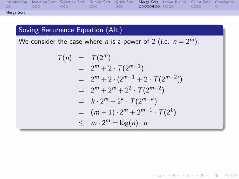
Soving Recurrence Equation (Alt.)
We consider the case where n is a power of 2 (i.e. n = 2m).
T (n) = T (2m)
= 2m + 2 · T (2m−1)
= 2m + 2 · (2m−1 + 2 · T (2m−2))
= 2m + 2m + 22 · T (2m−2)
= k · 2m + 2k · T (2m−k)
= (m − 1) · 2m + 2m−1 · T (21)
≤ m · 2m = log(n) · n
Introduction Insertion Sort Selection Sort Bubble Sort Quick Sort Merge Sort Lower Bound Count Sort Conclusion
Merge Sort
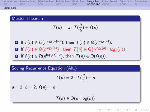
Master Theorem
T (n) = a · T (n
b) + f (n)
1 If f (n) ∈ O(nlogb(a)−ε), then T (n) ∈ Θ(nlogb(a)).
2 If f (n) ∈ Θ(nlogb(a)) , then T (n) ∈ Θ(nlogb(a) · logb(n))
3 If f (n) ∈ Ω(nlogb(a)+ε), then T (n) ∈ Θ(f (n)).
Soving Recurrence Equation (Alt.)
T (n) = 2 · T (n
2) + n
a = 2, b = 2, f (n) = n.
T (n) ∈ Θ(n · log(n))

Introduction Insertion Sort Selection Sort Bubble Sort Quick Sort Merge Sort Lower Bound Count Sort Conclusion
Merge Sort
Merge Sort
Worst case performance O(n log n).
Best case performance O(n log n).
Average case performance O(n log n).
Worst case space complexity O(n).

Introduction Insertion Sort Selection Sort Bubble Sort Quick Sort Merge Sort Lower Bound Count Sort Conclusion
Lower Bound
What can we Expect?
A sorting algorithm can compare, copy and move elements.No other information is available.
The running time of a sorting algorithm depends on thenumber of comparisons.

Introduction Insertion Sort Selection Sort Bubble Sort Quick Sort Merge Sort Lower Bound Count Sort Conclusion
Lower Bound
Sorting Two Elements
There are only two possible cases. One comparison allows sortingtwo elements.
If e1 ≤ e2 then (e1, e2) is sorted.
Else (e2, e1) is sorted.

Introduction Insertion Sort Selection Sort Bubble Sort Quick Sort Merge Sort Lower Bound Count Sort Conclusion
Lower Bound
Sorting Three Elements
There are only six possible cases. Three comparisons allow sortingthree elements.
If e1 ≤ e2 and e2 ≤ e3 and e1 ≤ e3 then (e1, e2, e3) is sorted.
If e1 ≤ e2 and e2 ≤ e3 and e3 < e1 is impossible.
If e1 ≤ e2 and e3 < e2 and e1 < e3 then (e1, e3, e2) is sorted.
If e1 ≤ e2 and e3 < e2 and e3 < e1 then (e3, e1, e2) is sorted.
If e2 < e1 and e2 < e3 and e1 < e3 then (e2, e1, e3) is sorted.
If e2 < e1 and e2 ≤ e3 and e3 < e1 then (e2, e3, e1) is sorted.
If e2 < e1 and e3 < e2 and e1 < e3 is impossible
If e2 < e1 and e3 < e2 and e3 < e1 then (e3, e2, e1) is sorted.

Introduction Insertion Sort Selection Sort Bubble Sort Quick Sort Merge Sort Lower Bound Count Sort Conclusion
Lower Bound
Sorting n Elements
There are n! possible cases (permutation of n elements).
With m comparisons we can cater for 2m cases (someimpossible).
We need m comparisons such that 2m ≥ n!.
n! > (n/2)n/2; thus log(n!) > log(n/2) · n/2.
Therefore m > n/2 · log(n/2).
Lower Bound
Sorting is Ω(n log(n)).

Introduction Insertion Sort Selection Sort Bubble Sort Quick Sort Merge Sort Lower Bound Count Sort Conclusion
Count Sort
Count Sort
If the list contains numbers between 0 and some known maximum,possibly with some duplicates, we count just count the number ofoccurrences of each number and insert each number as many timesas it occurs in the list in increasing order.

Introduction Insertion Sort Selection Sort Bubble Sort Quick Sort Merge Sort Lower Bound Count Sort Conclusion
Count Sort
1 f u n c t i o n c o u n t s o r t (A)2 va r i , j ;3 va r count = new Array ( ) ;4 f o r ( i i n A)5 count [A[ i ] ] = 0 ; 6 f o r ( i i n A)7 count [A[ i ] ]++; 8 va r B = new Array ( ) ; va r k=0;9 f o r ( i i n count )
10 f o r ( j =0; j<count [ i ] ; j++)11 B[ k ] = i ; k++; 12 r e t u r n B ; 13 // The loop ” f o r i i n count ” l e t s14 // i go i n a s c end i ng nume r i c a l o r d e r .
”code/count sort.js”
Load the sorting algorithm into a browser
Introduction Insertion Sort Selection Sort Bubble Sort Quick Sort Merge Sort Lower Bound Count Sort Conclusion
Count Sort
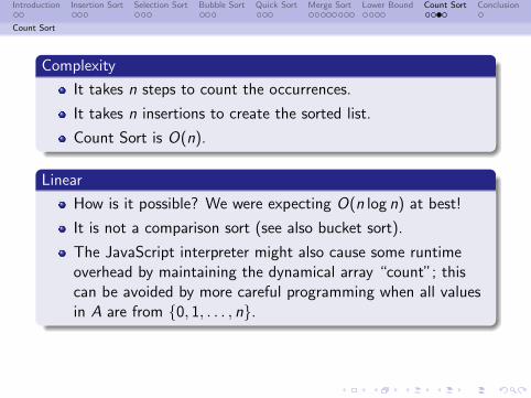
Complexity
It takes n steps to count the occurrences.
It takes n insertions to create the sorted list.
Count Sort is O(n).
Linear
How is it possible? We were expecting O(n log n) at best!
It is not a comparison sort (see also bucket sort).
The JavaScript interpreter might also cause some runtimeoverhead by maintaining the dynamical array “count”; thiscan be avoided by more careful programming when all valuesin A are from 0, 1, . . . , n.

Introduction Insertion Sort Selection Sort Bubble Sort Quick Sort Merge Sort Lower Bound Count Sort Conclusion
Count Sort
1 f u n c t i o n c o u n t s o r t (A)2 va r i , j ; v a r max = 0 ;3 f o r ( i i n A)4 i f (A [ i ]>max) max = A[ i ] ; 5 va r count = new Array (max+1) ;6 f o r ( i =0; i<=max ; i++)7 count [ i ] = 0 ; 8 f o r ( i i n A)9 count [A[ i ] ]++;
10 va r B = new Array ( ) ; va r k=0;11 f o r ( i =0; i<=max ; i++)12 f o r ( j =0; j<count [ i ] ; j++)13 B[ k ] = i ; k++; 14 r e t u r n B ; 15 // Run Time i s O(A . l e n g t h+max) ;
”code/count sort static.js”
Load the sorting algorithm into a browser

Introduction Insertion Sort Selection Sort Bubble Sort Quick Sort Merge Sort Lower Bound Count Sort Conclusion
Attribution
Attribution
The images and media files used in this presentation are either inthe public domain or are licensed under the terms of the GNU FreeDocumentation License, Version 1.2 or any later version publishedby the Free Software Foundation, the Creative CommonsAttribution-Share Alike 3.0 Unported license or the CreativeCommons Attribution-Share Alike 2.5 Generic, 2.0 Generic and 1.0Generic license.
Related Documents