Image Processing - Laboratory 9: Image filtering in the spatial and frequency domains 1 9. Image filtering in the spatial and frequency domains 9.1. Introduction In this laboratory the convolution operator will be presented. This operator is used in the linear image filtering process applied in the spatial domain (in the image plane by directly manipulating the pixels) or in the frequency domain (applying a Fourier transform, filtering and then applying the inverse Fourier transform. Examples of such filters are: low pass filters (for smoothing) and high pass filters (for edge enhancement). 9.2. The convolution process in the spatial domain The convolution process implies the usage of a convolution mask/kernel H (usually with symmetric shape and size ×, with w=2k+1) which is applied on the source image according to (9.2). (, ) = ∗ (9.1) (, ) = ∑ ∑ (, ) ⋅ ( + − , + − ) −1 =0 −1 =0 (9.2) This implies the scanning of the source image IS, pixel by pixel, ignoring the first and last k rows and columns (Fig. 9.1) and the computation of the intensity value in the current position (i, j) of the destination image ID using (9.2). The convolution mask is positioned spatially with its central element over the current position (i, j). Fig. 9.1 Illustration of the convolution process. The convolution kernels can have also non-symmetrical shapes (the central/reference element is not positioned in the center of symmetry). Convolution with such kernels is applied in a similar way, but such examples will not be presented in the current laboratory. 9.2.1. Low-pass filters Low-pass filters are used for image smoothing and noise reduction (see the lecture material). Their effect is an averaging of the current pixel with the values of its neighbors, observable as a “blurring” of the output image (they allow to pass only the low frequencies of the image). All elements of the kernels used for low-pass filtering have positive values. Therefore, a common practice used to scale the result in the intensity domain of the output image is to divide the result of the convolution with the sum of the elements of the kernel:

Welcome message from author
This document is posted to help you gain knowledge. Please leave a comment to let me know what you think about it! Share it to your friends and learn new things together.
Transcript
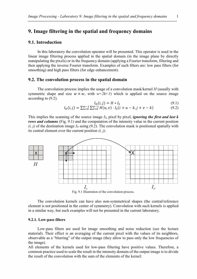
Image Processing - Laboratory 9: Image filtering in the spatial and frequency domains
1
9. Image filtering in the spatial and frequency domains
9.1. Introduction
In this laboratory the convolution operator will be presented. This operator is used in the
linear image filtering process applied in the spatial domain (in the image plane by directly
manipulating the pixels) or in the frequency domain (applying a Fourier transform, filtering and
then applying the inverse Fourier transform. Examples of such filters are: low pass filters (for
smoothing) and high pass filters (for edge enhancement).
9.2. The convolution process in the spatial domain
The convolution process implies the usage of a convolution mask/kernel H (usually with
symmetric shape and size 𝑤 ×𝑤, with w=2k+1) which is applied on the source image
according to (9.2).
𝐼𝐷(𝑖, 𝑗) = 𝐻 ∗ 𝐼𝑆 (9.1)
𝐼𝐷(𝑖, 𝑗) = ∑ ∑ 𝐻(𝑢, 𝑣) ⋅ 𝐼𝑆(𝑖 + 𝑢 − 𝑘, 𝑗 + 𝑣 − 𝑘)𝑤−1𝑣=0
𝑤−1𝑢=0 (9.2)
This implies the scanning of the source image IS, pixel by pixel, ignoring the first and last k
rows and columns (Fig. 9.1) and the computation of the intensity value in the current position
(i, j) of the destination image ID using (9.2). The convolution mask is positioned spatially with
its central element over the current position (i, j).
Fig. 9.1 Illustration of the convolution process.
The convolution kernels can have also non-symmetrical shapes (the central/reference
element is not positioned in the center of symmetry). Convolution with such kernels is applied
in a similar way, but such examples will not be presented in the current laboratory.
9.2.1. Low-pass filters
Low-pass filters are used for image smoothing and noise reduction (see the lecture
material). Their effect is an averaging of the current pixel with the values of its neighbors,
observable as a “blurring” of the output image (they allow to pass only the low frequencies of
the image).
All elements of the kernels used for low-pass filtering have positive values. Therefore, a
common practice used to scale the result in the intensity domain of the output image is to divide
the result of the convolution with the sum of the elements of the kernel:

Technical University of Cluj-Napoca, Computer Science Department
2
𝐼𝐷(𝑖, 𝑗) =1
𝑐∑ ∑ 𝐻(𝑢, 𝑣) ⋅ 𝐼𝑆(𝑖 + 𝑢 − 𝑘, 𝑗 + 𝑣 − 𝑘)𝑤−1
𝑣=0𝑤−1𝑢=0 (9.3)
where:
𝑐 = ∑ ∑ 𝐻(𝑢, 𝑣)𝑤−1𝑣=0
𝑤−1𝑢=0 (9.4)
Example kernel matrices:
Mean filter (3x3):
111
111
111
9
1 (9.5)
Gaussian filter (3x3):
121
242
121
16
1 (9.6)
a. b. c.
Fig. 9.2 a. Original image; b. Result obtained by applying a 3x3 mean filter. c. Result obtained by applying a 5x5
mean filter.
9.2.2. High-pass filters
These filters will highlight regions with step intensity variations, such as edges (will allow to
pass the high frequencies).
The kernels used for edge detection have the sum of their elements equal to 0:
Laplace filters (edge detection) (3x3):
010
141
010
(9.7)
or
111
181
111
(9.8)

Image Processing - Laboratory 9: Image filtering in the spatial and frequency domains
3
High-pass filters (3x3):
010
151
010
(9.9)
or
111
191
111
(9.10)
a. b. c.
Fig. 9.3 a. The result of applying the Laplace edge detection filter (9.8) on the original image (Fig. 9.2a); b. The
result of applying the Laplace edge detection filter (9.8) on the blurred image from Fig. 9.2b (previously filtered
with the 3x3 mean filter); c. The result obtained by filtering the original image with the high-pass filter (9.10)
9.3. Image filtering in the frequency domain
The 1D discrete Fourier transform (DFT) of an array of N real or complex numbers is an
array of N complex numbers, given by:
21
0
, 0... 1
jknN
N
k n
n
X x e k N
(9.11)
The inverse discrete Fourier transform (IDFT) is given by:
21
0
1, 0... 1
jknN
N
n k
k
x X e n NN
(9.12)
The 2D DFT is performed by applying the 1D DFT on each row of the input image and
then on each column of the previous result. The 2D IDTF is performed by applying the 1D
IDFT on each column of the DFT “image” and then on each row of the previous result. The set
of complex numbers which are the result of the DFT may also be represented in polar
coordinates (magnitude, phase). The set of (real) magnitudes represent the frequency power
spectrum of the original array.
The DFT and its inverse are usually performed using the Fast Fourier Transform recursive
approach, which reduces the computation time from 2( )O n to ( ln )O n n , which represents a
significant speed increase, especially in the case of 2D image processing, where a 2 2( )O n m
complexity would be intractable for large images as opposed to the almost linear in number of
pixels ( ln( ))O nm nm complexity.
Technical University of Cluj-Napoca, Computer Science Department
4
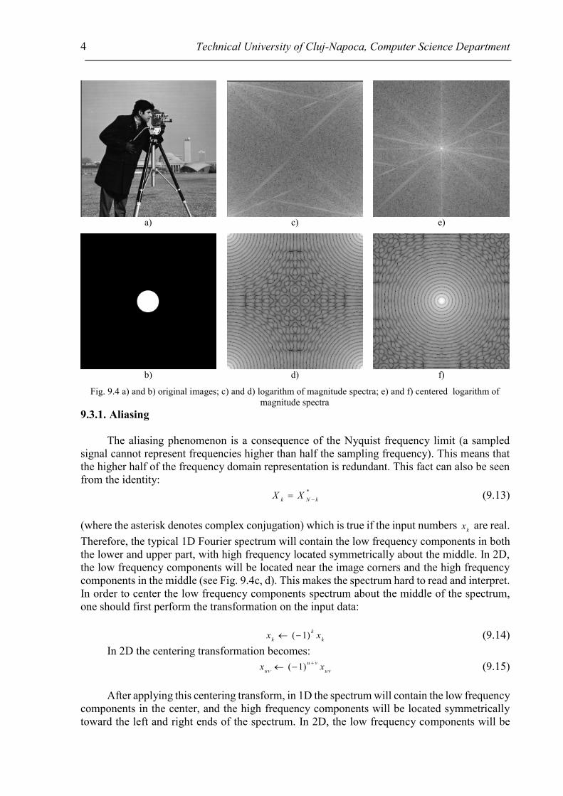
9.3.1. Aliasing
The aliasing phenomenon is a consequence of the Nyquist frequency limit (a sampled
signal cannot represent frequencies higher than half the sampling frequency). This means that
the higher half of the frequency domain representation is redundant. This fact can also be seen
from the identity:
*
k N kX X
(9.13)
(where the asterisk denotes complex conjugation) which is true if the input numbers k
x are real.
Therefore, the typical 1D Fourier spectrum will contain the low frequency components in both
the lower and upper part, with high frequency located symmetrically about the middle. In 2D,
the low frequency components will be located near the image corners and the high frequency
components in the middle (see Fig. 9.4c, d). This makes the spectrum hard to read and interpret.
In order to center the low frequency components spectrum about the middle of the spectrum,
one should first perform the transformation on the input data:
( 1)k
k kx x (9.14)
In 2D the centering transformation becomes:
( 1)u v
uv uvx x
(9.15)
After applying this centering transform, in 1D the spectrum will contain the low frequency
components in the center, and the high frequency components will be located symmetrically
toward the left and right ends of the spectrum. In 2D, the low frequency components will be
a)
c)
e)
b)
d)
f)
Fig. 9.4 a) and b) original images; c) and d) logarithm of magnitude spectra; e) and f) centered logarithm of
magnitude spectra

Image Processing - Laboratory 9: Image filtering in the spatial and frequency domains
5
located in the middle of the image, while various high frequency components will be located
toward the edges.
The magnitudes located on any line passing through the DFT image center represent the
1D frequency spectrum components of the original image, along the direction of the line. Every
such line is therefore symmetrical about its middle (the image center).
a)
b)
c)
d)
Fig. 9.5 Fourier transforms of sine image waves a) and c). The center point in b) and d) represent the DC
component, the other two symmetrical points are due to the sine wave frequency.
9.3.2. Ideal low-pass and high-pass filters in frequency domain
The convolution in spatial domain is equivalent to scalar multiplication in frequency
domain. Therefore, especially for large convolution kernels, it is computationally convenient to
perform convolution in the frequency domain.
The algorithm for filtering in the frequency domain is:
a) Perform the image centering transform on the original image (9.15)
b) Perform the DFT transform
c) Alter the Fourier coefficients according to the required filtering
d) Perform the IDFT transform
e) Perform the image centering transform again (this undoes the first centering transform).
An ideal low pass filter will alter all the Fourier coefficients that are further away from
the image center (W/2, H/2) than a given distance R, by turning them to zero (W is the image
width and H is the image height):
2 2
2
'
2 2
2
, 2 2
0 , 2 2
uv
uv
H WX u v R
X
H Wu v R
(9.16)
An ideal high-pass filter will alter all Fourier coefficients that are at a distance less than
R from the image center (W/2, H/2), by turning them to 0.
2 2
2
'
2 2
2
, 2 2
0 , 2 2
uv
uv
H WX u v R
X
H Wu v R
(9.17)

Technical University of Cluj-Napoca, Computer Science Department
6
The results of filtering with ideal low- and high-pass filtering are presented in Fig. 9.6 b)
and c). Unfortunately, the corresponding spatial filters Fig. 9.6 e) and d) are not FIR (they have
an infinite support) and keep oscillating away from their centers. Because of this, the low-pass
and high-pass filtered images have a disturbing ringing wavy aspect. In order to correct this,
the cutoff in the frequency domain must be smoother, as presented in the next section.
a)
b)
c)
d)
e)
f)
g)
Fig. 9.6 a) original image; b) result of ideal low-pass filtering; c) result of ideal high-pass filtering;
d) ideal low-pass filter in the frequency domain; e) corresponding ideal low-pass filter in the spatial
domain; f) ideal high-pass filter in the frequency domain; g) corresponding ideal high-pass filter
in the spatial domain
9.3.3. Gaussian low-pass and high-pass filtering in the frequency domain
In the case of Gaussian filtering, the frequency coefficients are not cut abruptly, but
smoother cutoff process is used instead. This also takes advantage of the fact that the DFT of a
Gaussian function is also a Gaussian function (Fig. 9.7d-g).
The Gaussian low-pass filter attenuates frequency components that are further away from the
image center (W/2, H/2). 1
~A
where is the standard deviation of the equivalent spatial
domain Gaussian filter.
2 2
2
2 2
'
H Wu v
A
uv uvX X e
(9.18)
The Gaussian high-pass filter attenuates frequency components that are near to the image
center (W/2, H/2):
2 2
2
2 2
'1
H Wu v
A
uv uvX X e
(9.19)
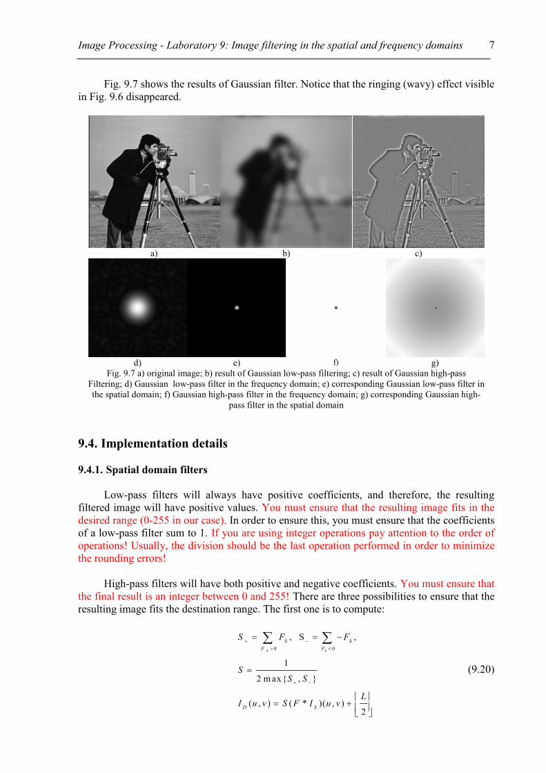
Image Processing - Laboratory 9: Image filtering in the spatial and frequency domains
7
Fig. 9.7 shows the results of Gaussian filter. Notice that the ringing (wavy) effect visible
in Fig. 9.6 disappeared.
a)
b)
c)
d)
e)
f)
g)
Fig. 9.7 a) original image; b) result of Gaussian low-pass filtering; c) result of Gaussian high-pass
Filtering; d) Gaussian low-pass filter in the frequency domain; e) corresponding Gaussian low-pass filter in
the spatial domain; f) Gaussian high-pass filter in the frequency domain; g) corresponding Gaussian high-
pass filter in the spatial domain
9.4. Implementation details
9.4.1. Spatial domain filters
Low-pass filters will always have positive coefficients, and therefore, the resulting
filtered image will have positive values. You must ensure that the resulting image fits in the
desired range (0-255 in our case). In order to ensure this, you must ensure that the coefficients
of a low-pass filter sum to 1. If you are using integer operations pay attention to the order of
operations! Usually, the division should be the last operation performed in order to minimize
the rounding errors!
High-pass filters will have both positive and negative coefficients. You must ensure that
the final result is an integer between 0 and 255! There are three possibilities to ensure that the
resulting image fits the destination range. The first one is to compute:
0 0
, S ,
1
2 m ax{ , }
( , ) ( * )( , )2
k k
k k
F F
D S
S F F
SS S
LI u v S F I u v
(9.20)
Technical University of Cluj-Napoca, Computer Science Department
8
In the formula above S
represents the sum of positive filter coefficients and S the sum
of negative filter coefficients magnitudes. This result of applying the high-pass filter always
lies in the interval [ , ]LS LS
where L is the maximum image gray level (255). The result of
this transform will place scale the result to [-L/2, L/2] and then move the 0 level to L/2.
Another approach is to perform all operations using signed integers determine the
minimum and maximum and then linearly transform the resulting values according to:
( min)
max min
L SD
(9.21)
The third approach is to compute the magnitude of the result and saturate everything that
exceeds the maximum level L.
9.4.2. Frequency domain filters
It is common practice for visualization and for processing purposes to consider a
representation of the frequency space which has the (0,0) coefficient in the image center. This
can be achieved by cross-swapping the four quadrants of the Fourier image channels.
Equivalently, we can preprocess the source image using 9.15. The generic filter presented below
uses the following helper function which performs the centering operation.
void centering_transform(Mat img){ //expects floating point image for (int i = 0; i < img.rows; i++){ for (int j = 0; j < img.cols; j++){ img.at<float>(i, j) = ((i + j) & 1) ? -img.at<float>(i, j) : img.at<float>(i, j); } } }
The OpenCV library provides an implementation for performing Discrete Fourier
Transform. The following template code performs both the direct and the inverse
transformation. Processing should be done on the magnitude channel of the Fourier transform.
Since DFT works best if the input image has dimensions equal to powers of two, use
cameraman.bmp as your input.
Mat generic_frequency_domain_filter(Mat src){
//convert input image to float image Mat srcf; src.convertTo(srcf, CV_32FC1); //centering transformation centering_transform(srcf); //perform forward transform with complex image output Mat fourier; dft(srcf, fourier, DFT_COMPLEX_OUTPUT); //split into real and imaginary channels Mat channels[] = { Mat::zeros(src.size(), CV_32F), Mat::zeros(src.size(), CV_32F) }; split(fourier, channels); // channels[0] = Re(DFT(I)), channels[1] = Im(DFT(I)) //calculate magnitude and phase in floating point images mag and phi Mat mag, phi; magnitude(channels[0], channels[1], mag); phase(channels[0], channels[1], phi); //display the phase and magnitude images here // ......

Image Processing - Laboratory 9: Image filtering in the spatial and frequency domains
9
//insert filtering operations on Fourier coefficients here // ......
//store in real part in channels[0] and imaginary part in channels[1] // ......
//perform inverse transform and put results in dstf Mat dst, dstf; merge(channels, 2, fourier); dft(fourier, dstf, DFT_INVERSE | DFT_REAL_OUTPUT | DFT_SCALE); //inverse centering transformation centering_transform(dstf); //normalize the result and put in the destination image normalize(dstf, dst, 0, 255, NORM_MINMAX, CV_8UC1); return dst; }
9.5. Practical work
1. Implement a general filter which performs the convolution operator with a custom
kernel matrix. The scaling coefficient should be computed automatically as either the
reciprocal of the sum of filter coefficients for low pass filters or according to equation
(9.20) for high-pass filters.
2. Test the filter with the kernels from equations (9.5) .... (9.10)
3. Study the provided generic function for processing in the frequency domain. Perform
the conversion of a source image from spatial domain to frequency domain by using the
Fourier transform (DFT), then apply the inverse Fourier transform (IDFT) on the
obtained Fourier spectrum coefficients and check if the destination is the same as the
source image.
4. Add a processing function that computes and displays the logarithm of the magnitude
of the Fourier transform of an input image. Add 1 to the magnitude to avoid log(0).
5. Add processing functions that perform low- and high-pass filtering in the frequency
domain using the ideal and Gaussian filters from equations (9.16)...(9.19).
6. Save your work. Use the same application in the next laboratories. At the end of
the image processing laboratory you should present your own application with the
implemented algorithms.
References
[1]. Umbaugh Scot E, Computer Vision and Image Processing, Prentice Hall, NJ, 1998, ISBN
0-13-264599-8
[2] R.C.Gonzales, R.E.Woods, Digital Image Processing, 2-nd Edition, Prentice Hall, 2002
Related Documents