Lecture Notes on Mathematical Systems Biology [Continuously revised and updated. This is version 5.0.5. Compiled September 24, 2011] Please address comments, suggestions, and corrections to the author. Eduardo D. Sontag, Rutgers University, c 2005,2006,2009,2010,2011 The first version of these notes dates back to 2005. They were originally heavily inspired by Leah Keshet’s beautiful book Mathematical Models in Biology (McGraw-Hill, 1988), and the reader will notice much material “borrowed” from there as well as other sources. In time, I changed the emphasis to be heavier on “systems biology” ideas and lighter on traditional population dynamics and ecology. (Topics like Lotka-Volterra predator-prey models are only done as problems, the assumption being that they have been covered as examples in a previous ODE course.) The goal was to provide students with an overview of the field. With more time, one would include much other material, such as Turing pattern-formation and detailed tissue modeling. The writing is not always textbook-like, but is sometimes “telegraphic” and streamlined, so as to make for easy reading and review. (The style is, however, not consistent, as the notes have been written over a long period.) Furthermore, I do not use “definition/theorem” rigorous mathematical style, so as to be more “user-friendly” to non-mathematicians. However, the reader can rest assured that every statement made can be cast as a theorem! Also, I tried to focus on intuitive and basic ideas, as opposed to going deeper into the beautiful theory that exists on ordinary and partial differential equation models in biology – for which many references exist. Please note that many figures are scanned from books or downloaded from the web, and their copy- right belongs to the respective authors, so please do not reproduce. Originally, the deterministic chapters (ODE and PDE) of these notes were prepared for the Rutgers course Math 336, Dynamical Models in Biology, which is a junior-level course designed for Biomath- ematics undergraduate majors, and attended as well by math, computer science, genetics, biomedical engineering, and other students. Math 336 does not cover discrete methods (genetics, DNA sequenc- ing, protein alignment, etc.), which are the subject of a companion course. With time, the notes were extended to include the chapter on stochastic kinetics, covered in Math 613, Mathematical Founda- tions of Systems Biology, a graduate course that also has an interdisciplinary audience. In its current version, the material no longer fits in a 1-semester course. Without the stochastic kinetics chapter, it should fit in one semester, though in practice, given time devoted to exam reviews, working out of homework problems, quizzes, etc., this is unrealistic. Pre-requisites for the deterministic part of notes are a solid foundation in calculus, up to and including sophomore ordinary differential equations, plus an introductory linear algebra course. Students should be familiar with basic qualitative ideas (phase line, phase plane) as well as simple methods such as separation of variables for scalar ODE’s. However, it may be possible to use these notes without the ODE and linear algebra prerequisites, provided that the student does some additional reading. The stochastic part requires good familiarity with basic probability theory. I am routinely asked if it is OK to use these notes in courses at other universities. The answer is, obviously, “of course!”. I do strongly suggest that a link to the my website be provided, so that students can access the current version. And please provide feedback!

87359342 Lecture Notes on Mathematical Systems Biology
Oct 26, 2014
Welcome message from author
This document is posted to help you gain knowledge. Please leave a comment to let me know what you think about it! Share it to your friends and learn new things together.
Transcript
Lecture Notes on Mathematical Systems Biology[Continuously revised and updated. This is version 5.0.5. Compiled September 24, 2011]
Please address comments, suggestions, and corrections to the author.
Eduardo D. Sontag, Rutgers University, c©2005,2006,2009,2010,2011
The first version of these notes dates back to 2005. They were originally heavily inspired by LeahKeshet’s beautiful book Mathematical Models in Biology (McGraw-Hill, 1988), and the reader willnotice much material “borrowed” from there as well as other sources. In time, I changed the emphasisto be heavier on “systems biology” ideas and lighter on traditional population dynamics and ecology.(Topics like Lotka-Volterra predator-prey models are only done as problems, the assumption beingthat they have been covered as examples in a previous ODE course.) The goal was to provide studentswith an overview of the field. With more time, one would include much other material, such as Turingpattern-formation and detailed tissue modeling.
The writing is not always textbook-like, but is sometimes “telegraphic” and streamlined, so as tomake for easy reading and review. (The style is, however, not consistent, as the notes have beenwritten over a long period.) Furthermore, I do not use “definition/theorem” rigorous mathematicalstyle, so as to be more “user-friendly” to non-mathematicians. However, the reader can rest assuredthat every statement made can be cast as a theorem! Also, I tried to focus on intuitive and basic ideas,as opposed to going deeper into the beautiful theory that exists on ordinary and partial differentialequation models in biology – for which many references exist.
Please note that many figures are scanned from books or downloaded from the web, and their copy-right belongs to the respective authors, so please do not reproduce.
Originally, the deterministic chapters (ODE and PDE) of these notes were prepared for the Rutgerscourse Math 336, Dynamical Models in Biology, which is a junior-level course designed for Biomath-ematics undergraduate majors, and attended as well by math, computer science, genetics, biomedicalengineering, and other students. Math 336 does not cover discrete methods (genetics, DNA sequenc-ing, protein alignment, etc.), which are the subject of a companion course. With time, the notes wereextended to include the chapter on stochastic kinetics, covered in Math 613, Mathematical Founda-tions of Systems Biology, a graduate course that also has an interdisciplinary audience. In its currentversion, the material no longer fits in a 1-semester course. Without the stochastic kinetics chapter, itshould fit in one semester, though in practice, given time devoted to exam reviews, working out ofhomework problems, quizzes, etc., this is unrealistic.
Pre-requisites for the deterministic part of notes are a solid foundation in calculus, up to and includingsophomore ordinary differential equations, plus an introductory linear algebra course. Students shouldbe familiar with basic qualitative ideas (phase line, phase plane) as well as simple methods such asseparation of variables for scalar ODE’s. However, it may be possible to use these notes without theODE and linear algebra prerequisites, provided that the student does some additional reading. Thestochastic part requires good familiarity with basic probability theory.
I am routinely asked if it is OK to use these notes in courses at other universities. The answer is,obviously, “of course!”. I do strongly suggest that a link to the my website be provided, so thatstudents can access the current version. And please provide feedback!

Eduardo D. Sontag, Lecture Notes on Mathematical Systems Biology 2
Acknowledgements
Obviously, these notes owe a lot to Leah Keshet’s book (which was out of print at the time when Istarted writing them, but has since been reprinted by SIAM).
In addition, many students have helped with questions, comments, and suggestions. I am especiallyindebted to Zahra Aminzare for helping out with writing problems.
Contents
1 Deterministic ODE models 7
1.1 Modeling, Growth, Number of Parameters . . . . . . . . . . . . . . . . . . . . . . . 7
1.1.1 Exponential Growth: Modeling . . . . . . . . . . . . . . . . . . . . . . . . 7
1.1.2 Exponential Growth: Math . . . . . . . . . . . . . . . . . . . . . . . . . . . 8
1.1.3 Limits to Growth: Modeling . . . . . . . . . . . . . . . . . . . . . . . . . . 8
1.1.4 Logistic Equation: Math . . . . . . . . . . . . . . . . . . . . . . . . . . . . 9
1.1.5 Changing Variables, Rescaling Time . . . . . . . . . . . . . . . . . . . . . . 10
1.1.6 A More Interesting Example: the Chemostat . . . . . . . . . . . . . . . . . 12
1.1.7 Chemostat: Mathematical Model . . . . . . . . . . . . . . . . . . . . . . . . 13
1.1.8 Michaelis-Menten Kinetics . . . . . . . . . . . . . . . . . . . . . . . . . . . 13
1.1.9 Side Remark: “Lineweaver-Burk plot” to Estimate Parameters . . . . . . . . 14
1.1.10 Chemostat: Reducing Number of Parameters . . . . . . . . . . . . . . . . . 14
1.2 Steady States and Linearized Stability Analysis . . . . . . . . . . . . . . . . . . . . 16
1.2.1 Steady States . . . . . . . . . . . . . . . . . . . . . . . . . . . . . . . . . . 16
1.2.2 Linearization . . . . . . . . . . . . . . . . . . . . . . . . . . . . . . . . . . 18
1.2.3 Review of (Local) Stability . . . . . . . . . . . . . . . . . . . . . . . . . . . 19
1.2.4 Chemostat: Local Stability . . . . . . . . . . . . . . . . . . . . . . . . . . . 21
1.3 More Modeling Examples . . . . . . . . . . . . . . . . . . . . . . . . . . . . . . . 22
1.3.1 Effect of Drug on Cells in an Organ . . . . . . . . . . . . . . . . . . . . . . 22
1.3.2 Compartmental Models . . . . . . . . . . . . . . . . . . . . . . . . . . . . . 23
1.4 Geometric Analysis: Vector Fields, Phase Planes . . . . . . . . . . . . . . . . . . . 24
1.4.1 Review: Vector Fields . . . . . . . . . . . . . . . . . . . . . . . . . . . . . 24
1.4.2 Review: Linear Phase Planes . . . . . . . . . . . . . . . . . . . . . . . . . . 24
1.4.3 Nullclines . . . . . . . . . . . . . . . . . . . . . . . . . . . . . . . . . . . . 26
1.4.4 Global Behavior . . . . . . . . . . . . . . . . . . . . . . . . . . . . . . . . 28
1.5 Epidemiology: SIRS Model . . . . . . . . . . . . . . . . . . . . . . . . . . . . . . 30
1.5.1 Analysis of Equations . . . . . . . . . . . . . . . . . . . . . . . . . . . . . 32
3
Eduardo D. Sontag, Lecture Notes on Mathematical Systems Biology 4
1.5.2 Interpreting σ . . . . . . . . . . . . . . . . . . . . . . . . . . . . . . . . . . 33
1.5.3 Nullcline Analysis . . . . . . . . . . . . . . . . . . . . . . . . . . . . . . . 33
1.5.4 Immunizations . . . . . . . . . . . . . . . . . . . . . . . . . . . . . . . . . 34
1.5.5 A Variation: STD’s . . . . . . . . . . . . . . . . . . . . . . . . . . . . . . . 34
1.6 Chemical Kinetics . . . . . . . . . . . . . . . . . . . . . . . . . . . . . . . . . . . . 36
1.6.1 Equations . . . . . . . . . . . . . . . . . . . . . . . . . . . . . . . . . . . . 37
1.6.2 Chemical Networks . . . . . . . . . . . . . . . . . . . . . . . . . . . . . . . 38
1.6.3 Introduction to Enzymatic Reactions . . . . . . . . . . . . . . . . . . . . . . 41
1.6.4 Differential Equations . . . . . . . . . . . . . . . . . . . . . . . . . . . . . 44
1.6.5 Quasi-Steady State Approximations and Michaelis-Menten Reactions . . . . 45
1.6.6 A quick intuition with nullclines . . . . . . . . . . . . . . . . . . . . . . . . 46
1.6.7 Fast and Slow Behavior . . . . . . . . . . . . . . . . . . . . . . . . . . . . 48
1.6.8 Singular Perturbation Analysis . . . . . . . . . . . . . . . . . . . . . . . . . 51
1.6.9 Inhibition . . . . . . . . . . . . . . . . . . . . . . . . . . . . . . . . . . . . 52
1.6.10 Allosteric Inhibition . . . . . . . . . . . . . . . . . . . . . . . . . . . . . . 54
1.6.11 A digression on gene expression . . . . . . . . . . . . . . . . . . . . . . . . 55
1.6.12 Cooperativity . . . . . . . . . . . . . . . . . . . . . . . . . . . . . . . . . . 56
1.7 Multi-Stability . . . . . . . . . . . . . . . . . . . . . . . . . . . . . . . . . . . . . . 59
1.7.1 Hyperbolic and Sigmoidal Responses . . . . . . . . . . . . . . . . . . . . . 59
1.7.2 Adding Positive Feedback . . . . . . . . . . . . . . . . . . . . . . . . . . . 61
1.7.3 Cell Differentiation and Bifurcations . . . . . . . . . . . . . . . . . . . . . . 62
1.7.4 Sigmoidal responses without cooperativity: Goldbeter-Koshland . . . . . . . 68
1.7.5 Bistability with two species . . . . . . . . . . . . . . . . . . . . . . . . . . 69
1.8 Periodic Behavior . . . . . . . . . . . . . . . . . . . . . . . . . . . . . . . . . . . . 71
1.8.1 Periodic Orbits and Limit Cycles . . . . . . . . . . . . . . . . . . . . . . . . 72
1.8.2 An Example of Limit Cycle . . . . . . . . . . . . . . . . . . . . . . . . . . 72
1.8.3 Poincare-Bendixson Theorem . . . . . . . . . . . . . . . . . . . . . . . . . 73
1.8.4 The Van der Pol Oscillator . . . . . . . . . . . . . . . . . . . . . . . . . . . 75
1.8.5 Bendixson’s Criterion . . . . . . . . . . . . . . . . . . . . . . . . . . . . . 77
1.9 Bifurcations . . . . . . . . . . . . . . . . . . . . . . . . . . . . . . . . . . . . . . . 78
1.9.1 How can stability be lost? . . . . . . . . . . . . . . . . . . . . . . . . . . . 78
1.9.2 One real eigenvalue moves . . . . . . . . . . . . . . . . . . . . . . . . . . . 79
1.9.3 Hopf Bifurcations . . . . . . . . . . . . . . . . . . . . . . . . . . . . . . . . 81
1.9.4 Combinations of bifurcations . . . . . . . . . . . . . . . . . . . . . . . . . . 84
1.9.5 Cubic Nullclines and Relaxation Oscillations . . . . . . . . . . . . . . . . . 86
Eduardo D. Sontag, Lecture Notes on Mathematical Systems Biology 5
1.9.6 A Qualitative Analysis using Cubic Nullclines . . . . . . . . . . . . . . . . 88
1.9.7 Neurons . . . . . . . . . . . . . . . . . . . . . . . . . . . . . . . . . . . . . 89
1.9.8 Action Potential Generation . . . . . . . . . . . . . . . . . . . . . . . . . . 90
1.9.9 Model . . . . . . . . . . . . . . . . . . . . . . . . . . . . . . . . . . . . . . 93
1.10 Problems for ODE chapter . . . . . . . . . . . . . . . . . . . . . . . . . . . . . . . 97
1.10.1 Population growth . . . . . . . . . . . . . . . . . . . . . . . . . . . . . . . 97
1.10.2 Interacting population problems . . . . . . . . . . . . . . . . . . . . . . . . 98
1.10.3 Chemostat problems . . . . . . . . . . . . . . . . . . . . . . . . . . . . . . 102
1.10.4 Chemotherapy and other metabolism and drug infusion problems . . . . . . 106
1.10.5 Epidemiology problems . . . . . . . . . . . . . . . . . . . . . . . . . . . . 108
1.10.6 Chemical kinetics problems . . . . . . . . . . . . . . . . . . . . . . . . . . 111
1.10.7 Multiple steady states, sigmoidal responses, etc. problems . . . . . . . . . . 114
1.10.8 Oscillations and excitable systems problems . . . . . . . . . . . . . . . . . . 117
2 Deterministic PDE Models 1232.1 Introduction to PDE models . . . . . . . . . . . . . . . . . . . . . . . . . . . . . . 123
2.1.1 Densities . . . . . . . . . . . . . . . . . . . . . . . . . . . . . . . . . . . . 123
2.1.2 Reaction Term: Creation or Degradation Rate . . . . . . . . . . . . . . . . . 124
2.1.3 Conservation or Balance Principle . . . . . . . . . . . . . . . . . . . . . . . 124
2.1.4 Local fluxes: transport, chemotaxis . . . . . . . . . . . . . . . . . . . . . . 127
2.1.5 Transport Equation . . . . . . . . . . . . . . . . . . . . . . . . . . . . . . . 127
2.1.6 Solution for Constant Velocity and Exponential Growth or Decay . . . . . . 129
2.1.7 Attraction, Chemotaxis . . . . . . . . . . . . . . . . . . . . . . . . . . . . . 131
2.2 Non-local fluxes: diffusion . . . . . . . . . . . . . . . . . . . . . . . . . . . . . . . 136
2.2.1 Time of Diffusion (in dimension 1) . . . . . . . . . . . . . . . . . . . . . . 138
2.2.2 Another Interpretation of Diffusion Times (in dimension one) . . . . . . . . 139
2.2.3 Separation of Variables . . . . . . . . . . . . . . . . . . . . . . . . . . . . . 139
2.2.4 Examples of Separation of Variables . . . . . . . . . . . . . . . . . . . . . . 141
2.2.5 No-flux Boundary Conditions . . . . . . . . . . . . . . . . . . . . . . . . . 144
2.2.6 Probabilistic Interpretation . . . . . . . . . . . . . . . . . . . . . . . . . . . 145
2.2.7 Another Diffusion Example: Population Growth . . . . . . . . . . . . . . . 146
2.2.8 Systems of PDE’s . . . . . . . . . . . . . . . . . . . . . . . . . . . . . . . . 148
2.3 Steady-State Behavior of PDE’s . . . . . . . . . . . . . . . . . . . . . . . . . . . . 149
2.3.1 Steady State for Laplace Equation on Some Simple Domains . . . . . . . . . 150
2.3.2 Steady States for a Diffusion/Chemotaxis Model . . . . . . . . . . . . . . . 153
2.3.3 Facilitated Diffusion . . . . . . . . . . . . . . . . . . . . . . . . . . . . . . 154
Eduardo D. Sontag, Lecture Notes on Mathematical Systems Biology 6
2.3.4 Density-Dependent Dispersal . . . . . . . . . . . . . . . . . . . . . . . . . 156
2.4 Traveling Wave Solutions of Reaction-Diffusion Systems . . . . . . . . . . . . . . . 159
2.5 Problems for PDE chapter . . . . . . . . . . . . . . . . . . . . . . . . . . . . . . . 162
2.5.1 Transport problems . . . . . . . . . . . . . . . . . . . . . . . . . . . . . . . 162
2.5.2 Chemotaxis problems . . . . . . . . . . . . . . . . . . . . . . . . . . . . . 163
2.5.3 Diffusion problems . . . . . . . . . . . . . . . . . . . . . . . . . . . . . . . 164
2.5.4 Diffusion travelling wave problems problems . . . . . . . . . . . . . . . . . 167
2.5.5 General PDE modeling problems . . . . . . . . . . . . . . . . . . . . . . . 167
3 Stochastic kinetics 1713.1 Introduction . . . . . . . . . . . . . . . . . . . . . . . . . . . . . . . . . . . . . . . 171
3.2 Stochastic models of chemical reactions . . . . . . . . . . . . . . . . . . . . . . . . 173
3.3 The Chemical Master Equation . . . . . . . . . . . . . . . . . . . . . . . . . . . . . 174
3.3.1 Propensity functions for mass-action kinetics . . . . . . . . . . . . . . . . . 175
3.3.2 Some examples . . . . . . . . . . . . . . . . . . . . . . . . . . . . . . . . . 176
3.4 Theoretical background, algorithms, and discussion . . . . . . . . . . . . . . . . . . 179
3.4.1 Markov Processes . . . . . . . . . . . . . . . . . . . . . . . . . . . . . . . 179
3.4.2 The jump time process: how long do we wait until the next reaction? . . . . 180
3.4.3 Propensities . . . . . . . . . . . . . . . . . . . . . . . . . . . . . . . . . . . 182
3.4.4 Interpretation of the Master Equation and propensity functions . . . . . . . . 183
3.4.5 The embedded jump chain . . . . . . . . . . . . . . . . . . . . . . . . . . . 185
3.4.6 The stochastic simulation algorithm (SSA) . . . . . . . . . . . . . . . . . . 185
3.4.7 Interpretation of mass-action kinetics . . . . . . . . . . . . . . . . . . . . . 187
3.5 Moment equations and fluctuation-dissipation formula . . . . . . . . . . . . . . . . 190
3.5.1 Means . . . . . . . . . . . . . . . . . . . . . . . . . . . . . . . . . . . . . . 191
3.5.2 Variances . . . . . . . . . . . . . . . . . . . . . . . . . . . . . . . . . . . . 192
3.5.3 Reactions or order ≤ 1 or ≤ 2 . . . . . . . . . . . . . . . . . . . . . . . . . 194
3.6 Generating functions . . . . . . . . . . . . . . . . . . . . . . . . . . . . . . . . . . 196
3.7 Examples computed using the fluctuation-dissipation formula . . . . . . . . . . . . . 199
3.8 Conservation laws and stoichiometry . . . . . . . . . . . . . . . . . . . . . . . . . . 203
3.9 Relations to deterministic equations, and approximations . . . . . . . . . . . . . . . 205
3.9.1 Deterministic chemical equations . . . . . . . . . . . . . . . . . . . . . . . 205
3.9.2 Unit Poisson representation . . . . . . . . . . . . . . . . . . . . . . . . . . 207
3.9.3 Diffusion approximation . . . . . . . . . . . . . . . . . . . . . . . . . . . . 209
3.9.4 Relation to deterministic equation . . . . . . . . . . . . . . . . . . . . . . . 210
3.10 Problems for stochastic kinetics . . . . . . . . . . . . . . . . . . . . . . . . . . . . 212
Chapter 1
Deterministic ODE models
1.1 Modeling, Growth, Number of Parameters
Let us start by reviewing a subject treated in basic differential equations courses, namely how onederives differential equations for simple exponential growth and other simple models.
1.1.1 Exponential Growth: Modeling
Suppose that N(t) counts the population of a microorganism in culture, at time t, and write theincrement in a time interval [t, t+ h] as “g(N(t), h)”, so that we have:
N(t+ h) = N(t) + g(N(t), h) .
(The increment depends on the previous N(t), as well as on the length of the time interval.)
We expand g using a Taylor series to second order:
g(N, h) = a+ bN + ch+ eN2 + fh2 +KNh + cubic and higher order terms
(a, b, . . . are some constants). Observe that
g(0, h) ≡ 0 and g(N, 0) ≡ 0 ,
since there is no increment if there is no population or if no time has elapsed. The first condition tellsus that
a+ ch+ fh2 + . . . ≡ 0 ,
for all h, so a = c = f = 0, and the second condition (check!) says that also b = N = 0.Thus, we conclude that:
g(N, h) = KNh + cubic and higher order terms.
So, for h and N small:N(t+ h) = N(t) +KN(t)h , (1.1)
which says that
7
Eduardo D. Sontag, Lecture Notes on Mathematical Systems Biology 8
the increase in population during a (small) time intervalis proportional to the interval length and initial population size.
This means, for example, that if we double the initial population or if we double the interval,the resulting population growth is doubled.
Obviously, (1.1) should not be expected to be true for large h, because of “compounding” effects.It may or may not be true for large N , as we will discuss later.
We next explore the consequences of assuming Equation (1.1) holds for all small h>0 and all N .
As usual in applied mathematics, the “proof is in the pudding”:one makes such an assumption, explores mathematical consequences that follow from it,and generates predictions to be validated experimentally.If the predictions pan out, we might want to keep the model.If they do not, it is back to the drawing board and a new model has to be developed!
1.1.2 Exponential Growth: Math
From our approximationKN(t)h = N(t+ h)−N(t)
we have that
KN(t) =1
h(N(t+ h)−N(t))
Taking the limit as h → 0, and remembering the definition of derivative, we conclude that the right-
hand side converges todN
dt(t). We conclude that N satisfies the following differential equation:
dN
dt= KN . (1.2)
We may solve this equation by the method of separation of variables, as follows:
dN
N= Kdt ⇒
∫dN
N=
∫K dt ⇒ lnN = Kt+ c .
Evaluating at t = 0, we have lnN0 = c, so that ln(N(t)/N0) = Kt. Taking exponentials, we have:
N(t) = N0eKt (exponential growth: Malthus, 1798)
Bacterial populations tend to growth exponentially, so long as enough nutrients are available.
1.1.3 Limits to Growth: Modeling
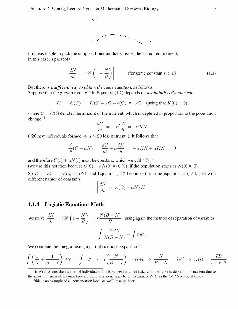
Suppose now there is some number B (the carrying capacity of the environment) so thatpopulations N > B are not sustainable, i.e.. dN/dt < 0 whenever N = N(t) > B:
Eduardo D. Sontag, Lecture Notes on Mathematical Systems Biology 9
It is reasonable to pick the simplest function that satisfies the stated requirement;in this case, a parabola:
dN
dt= rN
(1− N
B
)(for some constant r > 0) (1.3)
But there is a different way to obtain the same equation, as follows.Suppose that the growth rate “K” in Equation (1.2) depends on availability of a nutrient:
K = K(C) = K(0) + κC + o(C) ≈ κC (using that K(0) = 0)
where C = C(t) denotes the amount of the nutrient, which is depleted in proportion to the populationchange: 1
dC
dt= −αdN
dt= −αKN
(“20 new individuals formed⇒ α× 20 less nutrient”). It follows that
d
dt(C + αN) =
dC
dt+ α
dN
dt= −αKN + αKN = 0
and therefore C(t) + αN(t) must be constant, which we call “C0”2
(we use this notation because C(0) + αN(0) ≈ C(0), if the population starts as N(0) ≈ 0).
So K = κC = κ(C0 − αN), and Equation (1.2) becomes the same equation as (1.3), just withdifferent names of constants:
dN
dt= κ (C0 − αN)N
1.1.4 Logistic Equation: Math
We solvedN
dt= rN
(1− N
B
)= r
N(B −N)
Busing again the method of separation of variables:
∫B dN
N(B −N)=
∫r dt .
We compute the integral using a partial fractions expansion:∫ (1
N+
1
B −N
)dN =
∫r dt ⇒ ln
(N
B −N
)= rt+c ⇒ N
B −N= cert ⇒ N(t) =
cB
c+ e−rt
1if N(t) counts the number of individuals, this is somewhat unrealistic, as it the ignores depletion of nutrient due tothe growth or individuals once they are born; it is sometimes better to think of N(t) as the total biomass at time t
2this is an example of a “conservation law”, as we’ll discuss later
Eduardo D. Sontag, Lecture Notes on Mathematical Systems Biology 10
⇒ c = N0/(B −N0) ⇒ N(t) =N0B
N0 + (B −N0)e−rt
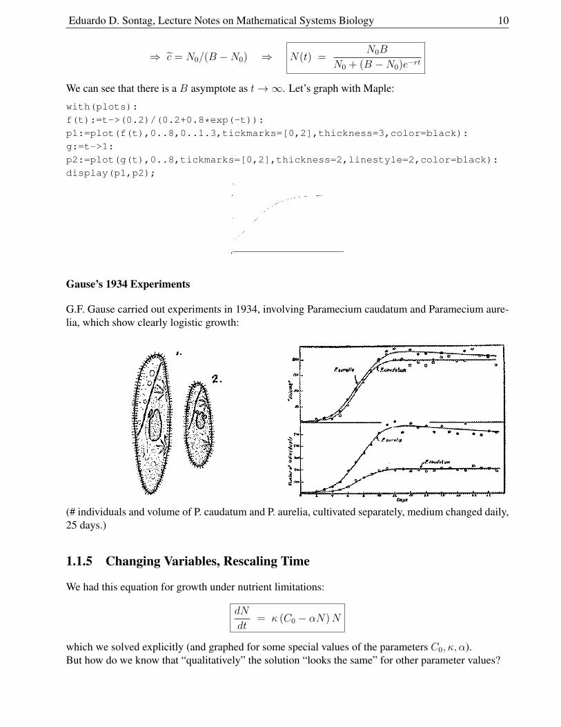
We can see that there is a B asymptote as t→∞. Let’s graph with Maple:
with(plots):
f(t):=t->(0.2)/(0.2+0.8*exp(-t)):
p1:=plot(f(t),0..8,0..1.3,tickmarks=[0,2],thickness=3,color=black):
g:=t->1:
p2:=plot(g(t),0..8,tickmarks=[0,2],thickness=2,linestyle=2,color=black):
display(p1,p2);
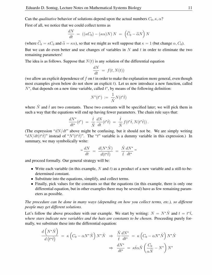
Gause’s 1934 Experiments
G.F. Gause carried out experiments in 1934, involving Paramecium caudatum and Paramecium aure-lia, which show clearly logistic growth:
(# individuals and volume of P. caudatum and P. aurelia, cultivated separately, medium changed daily,25 days.)
1.1.5 Changing Variables, Rescaling Time
We had this equation for growth under nutrient limitations:
dN
dt= κ (C0 − αN)N
which we solved explicitly (and graphed for some special values of the parameters C0, κ, α).But how do we know that “qualitatively” the solution “looks the same” for other parameter values?
Eduardo D. Sontag, Lecture Notes on Mathematical Systems Biology 11
Can the qualitative behavior of solutions depend upon the actual numbers C0, κ, α?
First of all, we notice that we could collect terms asdN
dt= ((κC0)− (κα)N)N =
(C0 − αN
)N
(where C0 = κC0 and α = κα), so that we might as well suppose that κ = 1 (but change α,C0).
But we can do even better and use changes of variables in N and t in order to eliminate the tworemaining parameters!
The idea is as follows. Suppose that N(t) is any solution of the differential equation
dN
dt= f(t, N(t))
(we allow an explicit dependence of f on t in order to make the explanation more general, even thoughmost examples given below do not show an explicit t). Let us now introduce a new function, calledN∗, that depends on a new time variable, called t∗, by means of the following definition:
N∗(t∗) :=1
NN(t∗t)
where N and t are two constants. These two constants will be specified later; we will pick them insuch a way that the equations will end up having fewer parameters. The chain rule says that:
dN∗
dt∗(t∗) =
t
N
dN
dt(t∗t) =
t
Nf(t∗t, N(t∗t)) .
(The expression “dN/dt” above might be confusing, but it should not be. We are simply writing“dN/dt(t∗t)” instead of “N ′(t∗t)”. The “t” variable is a dummy variable in this expression.) Insummary, we may symbolically write:
“dN
dt=
d(N∗N)
d(t∗t)=
N
t
dN∗
dt∗”
and proceed formally. Our general strategy will be:
• Write each variable (in this example, N and t) as a product of a new variable and a still-to-be-determined constant.• Substitute into the equations, simplify, and collect terms.• Finally, pick values for the constants so that the equations (in this example, there is only one
differential equation, but in other examples there may be several) have as few remaining param-eters as possible.
The procedure can be done in many ways (depending on how you collect terms, etc.), so differentpeople may get different solutions.
Let’s follow the above procedure with our example. We start by writing: N = N∗N and t = t∗t,where stars indicate new variables and the hats are constants to be chosen. Proceeding purely for-mally, we substitute these into the differential equation:
d(N∗N
)d(t∗t) = κ
(C0 − αN∗N
)N∗N ⇒ N
t
dN∗
dt∗= κ
(C0 − αN∗N
)N∗N
⇒ dN∗
dt∗= κtαN
(C0
αN−N∗
)N∗
Eduardo D. Sontag, Lecture Notes on Mathematical Systems Biology 12
Let us look at this last equation: we’d like to make C0
αN= 1 and κtαN = 1.
But this can be done! Just pick: N :=C0
αand t =
1
καN, that is: t :=
1
κC0
;dN∗
dt= (1−N∗)N∗ or, drop stars, and write just
dN
dt= (1−N)N
Thus, we can analyze the simpler system.
However, we should remember that the new “N” and “t” are rescaled versions of the old ones. Inorder to understand how to bring everything back to the original coordinates, note that another way toexpress the relation between N and N∗ is as follows:
N(t) = NN∗(t
t
)This formula allows us to recover the solutionN(t) to the original problem once that we have obtainedthe solution to the problem in the N∗, t∗ coordinates. That is to say, we may solve the equationdNdt
= (1−N)N , plot its solution, and then interpret the plot in original variables as a “stretching”of the plot in the new variables. Concretely, in our example:
N(t) =C0
αN∗ (κC0t)
(We may think of N∗, t∗ as quantity & time in some new units of measurement. This procedure isrelated to “nondimensionalization” of equations, which we’ll mention later.)
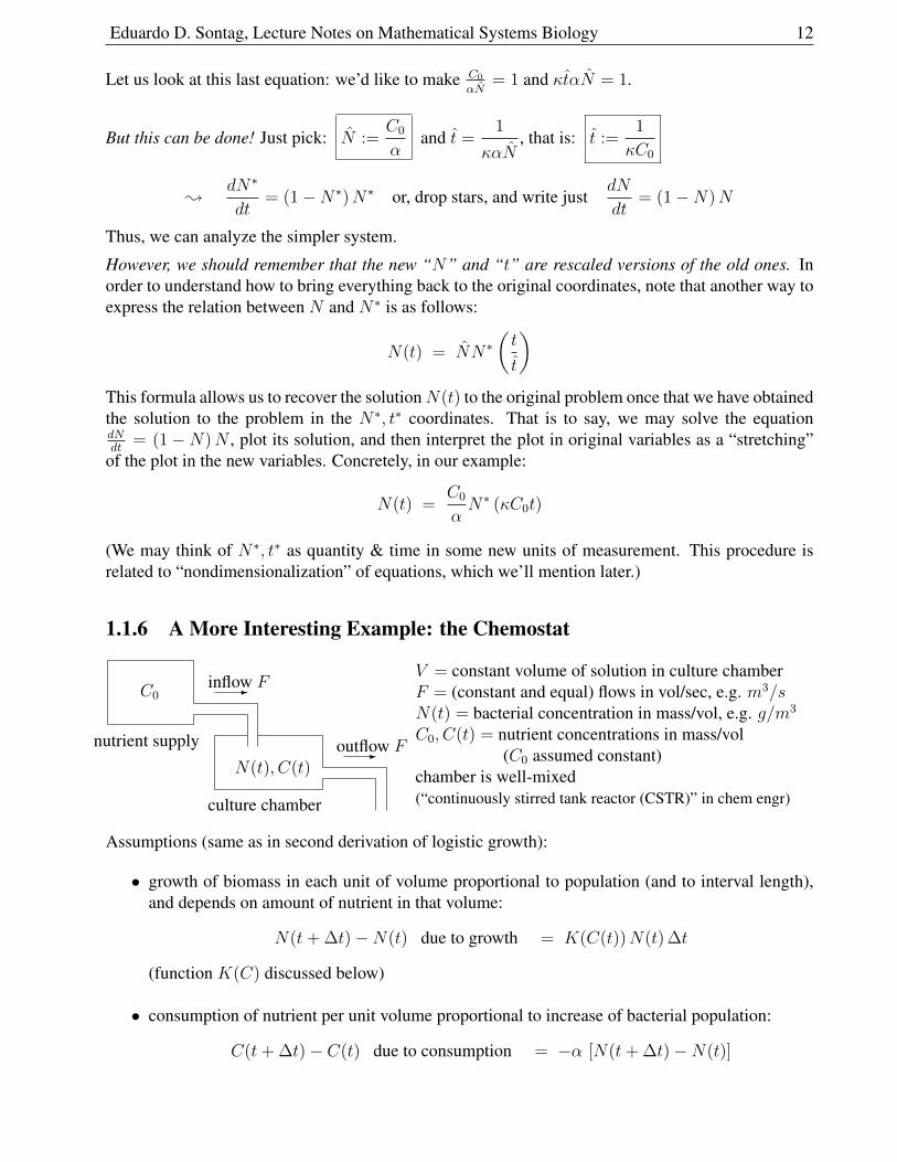
1.1.6 A More Interesting Example: the Chemostat
-
-nutrient supply
culture chamber
C0
N(t), C(t)
inflow F
outflow F
V = constant volume of solution in culture chamberF = (constant and equal) flows in vol/sec, e.g. m3/sN(t) = bacterial concentration in mass/vol, e.g. g/m3
C0, C(t) = nutrient concentrations in mass/vol(C0 assumed constant)
chamber is well-mixed(“continuously stirred tank reactor (CSTR)” in chem engr)
Assumptions (same as in second derivation of logistic growth):
• growth of biomass in each unit of volume proportional to population (and to interval length),and depends on amount of nutrient in that volume:
N(t+ ∆t)−N(t) due to growth = K(C(t))N(t) ∆t
(function K(C) discussed below)
• consumption of nutrient per unit volume proportional to increase of bacterial population:
C(t+ ∆t)− C(t) due to consumption = −α [N(t+ ∆t)−N(t)]
Eduardo D. Sontag, Lecture Notes on Mathematical Systems Biology 13
1.1.7 Chemostat: Mathematical Model
total biomass: N(t)V and total nutrient in culture chamber: C(t)V
biomass change in interval ∆t due to growth:
N(t+ ∆t)V −N(t)V = [N(t+ ∆t)−N(t)]V = K(C(t))N(t) ∆t V
so contribution to d(NV )/dt is “+K(C)NV ”
bacterial mass in effluent:in a small interval ∆t, the volume out is: F ·∆t (m
3
ss =)m3
so, since the concentration is N(t) g/m3, the mass out is: N(t) · F ·∆t gand so the contribution to d(NV )/dt is “−N(t)F ”
for d(CV )/dt equation:we have three terms: −αK(C)NV (depletion), −C(t)F (outflow), and +C0F (inflow), ;
d(NV )
dt= K(C)NV −NF
d(CV )
dt= −αK(C)NV − CF + C0F .
Finally, divide by the constant V to get this system of equations on N,C:
dN
dt= K(C)N −NF/V
dC
dt= −αK(C)N − CF/V + C0F/V
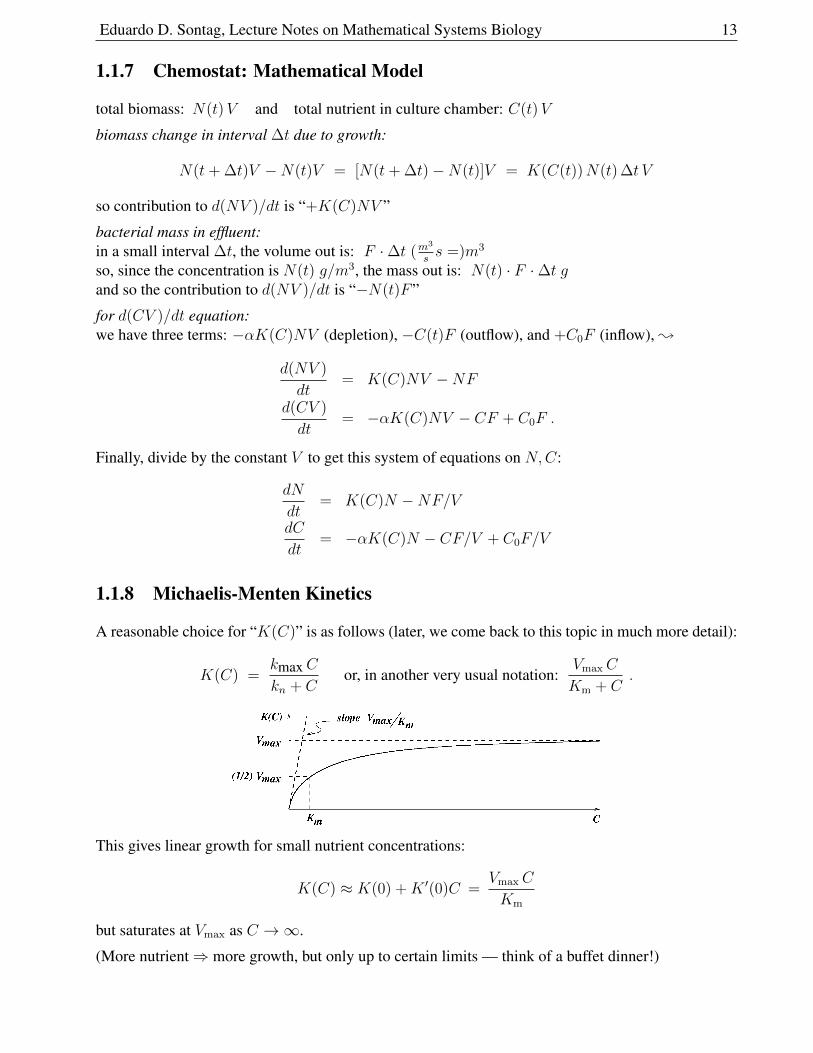
1.1.8 Michaelis-Menten Kinetics
A reasonable choice for “K(C)” is as follows (later, we come back to this topic in much more detail):
K(C) =kmaxCkn + C
or, in another very usual notation:VmaxC
Km + C.
This gives linear growth for small nutrient concentrations:
K(C) ≈ K(0) +K ′(0)C =VmaxC
Km
but saturates at Vmax as C →∞.
(More nutrient⇒ more growth, but only up to certain limits — think of a buffet dinner!)
Eduardo D. Sontag, Lecture Notes on Mathematical Systems Biology 14
Note that when C = Km, the growth rate is 1/2 (“m” for middle) of maximal, i.e. Vmax/2,
We thus have these equations for the chemostat with MM Kinetics:
dN
dt=
kmaxCkn + C
N − (F/V )N
dC
dt= −α kmaxC
kn + CN − (F/V )C + (F/V )C0
Our next goal is to study the behavior of this system of two ODE’sfor all possible values of the six parameters kmax, kn, F, V, C0, α.
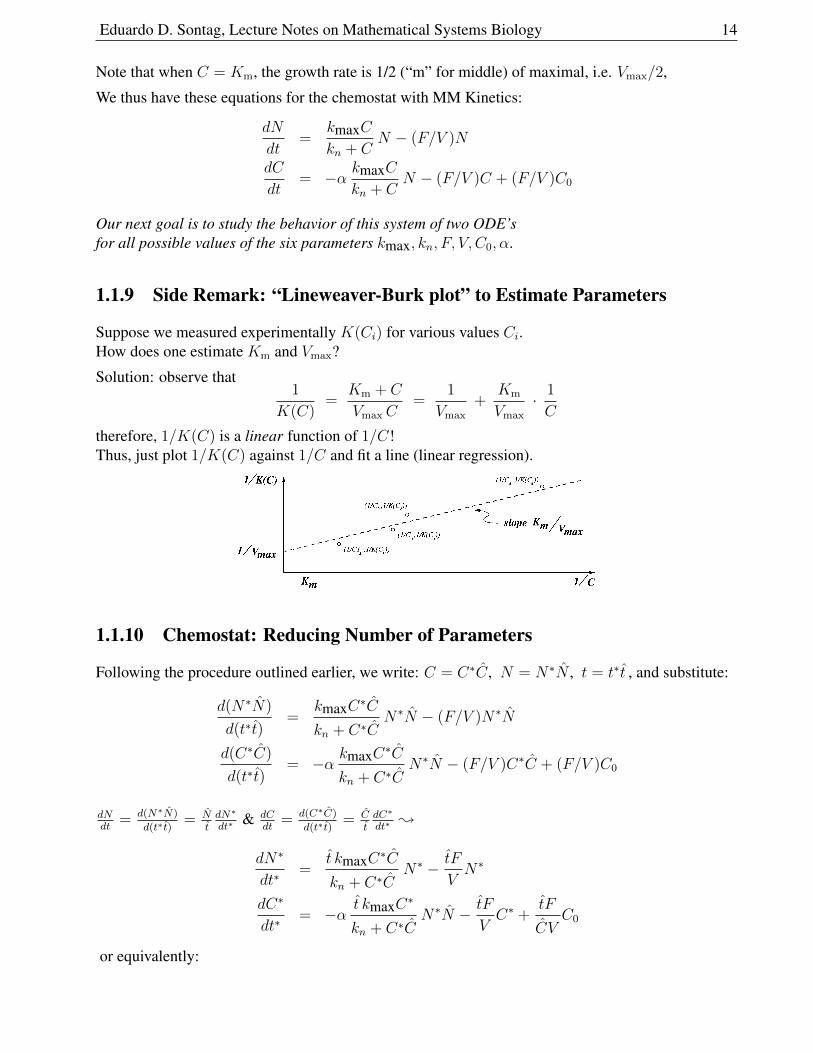
1.1.9 Side Remark: “Lineweaver-Burk plot” to Estimate Parameters
Suppose we measured experimentally K(Ci) for various values Ci.How does one estimate Km and Vmax?
Solution: observe that1
K(C)=
Km + C
VmaxC=
1
Vmax
+Km
Vmax
· 1
C
therefore, 1/K(C) is a linear function of 1/C!Thus, just plot 1/K(C) against 1/C and fit a line (linear regression).
1.1.10 Chemostat: Reducing Number of Parameters
Following the procedure outlined earlier, we write: C = C∗C, N = N∗N , t = t∗t , and substitute:
d(N∗N)
d(t∗t)=
kmaxC∗C
kn + C∗CN∗N − (F/V )N∗N
d(C∗C)
d(t∗t)= −α kmaxC∗C
kn + C∗CN∗N − (F/V )C∗C + (F/V )C0
dNdt
= d(N∗N)
d(t∗ t)= N
tdN∗
dt∗& dC
dt= d(C∗C)
d(t∗ t)= C
tdC∗
dt∗;
dN∗
dt∗=
t kmaxC∗C
kn + C∗CN∗ − tF
VN∗
dC∗
dt∗= −α t kmaxC∗
kn + C∗CN∗N − tF
VC∗ +
tF
CVC0
or equivalently:
Eduardo D. Sontag, Lecture Notes on Mathematical Systems Biology 15
dN∗
dt∗= (t kmax)
C∗
kn/C + C∗N∗ − tF
VN∗
dC∗
dt∗= −
(αt kmaxN
C
)C∗
kn/C + C∗N∗ − tF
VC∗ +
tF
CVC0
It would be nice, for example, to make kn/C = 1,tF
V= 1, and
αt kmaxN
C= 1. This can indeed be
done, provided that we define: C := kn, t :=V
F, and N :=
C
αt kmax=
kn
αt kmax=
knF
αV kmax
;dN∗
dt∗=
(V kmaxF
)C∗
1 + C∗N∗ −N∗
dC∗
dt∗= − C∗
1 + C∗N∗ − C∗ +
C0
kn
or, dropping stars and introducing two new constants α1 =(V kmax
F
)and α2 =
C0
knwe end up with:
dN
dt= α1
C
1 + CN −N
dC
dt= − C
1 + CN − C + α2
We will study how the behavior of the chemostat depends on these two parameters, always remember-ing to “translate back” into the original parameters and units.
The old and new variables are related as follows:
N(t) = NN∗(t
t
)=
knF
αV kmaxN∗(F
Vt
), C(t) = CC∗
(t
t
)= knC
∗(F
Vt
)
Remark on units
Since kmax is a rate (obtained at saturation), it has units time−1; thus, α1 is “dimensionless”.Similarly, kn has units of concentration (since it is being added to C, and in fact for C = kn we obtainhalf of the max rate kmax), so also α2 is dimensionless.
Dimensionless constants are a nice thing to have, since then we can talk about their being “small” or“large”. (What does it mean to say that a person of height 2 is tall? 2 cm? 2in? 2 feet? 2 meters?) Wedo not have time to cover the topic of units and non-dimensionalization in this course, however.
Eduardo D. Sontag, Lecture Notes on Mathematical Systems Biology 16
1.2 Steady States and Linearized Stability Analysis
1.2.1 Steady States
The key to the “geometric” analysis of systems of ODE’s is to write them in vector form:
dX
dt= F (X) (where F is a vector function and X is a vector) .
The vector X = X(t) has some number n of components, each of which is a function of time.One writes the components as xi (i = 1, 2, 3, . . . , n), or when n = 2 or n = 3 as x, y or x, y, z,or one uses notations that are related to the problem being studied, like N and C for the concentration(or the biomass) of a population and C for the concentration of a nutrient.For example, the chemostat
dN
dt= α1
C
1 + CN −N
dC
dt= − C
1 + CN − C + α2
may be written asdX
dt= F (X) =
(f(N,C)g(N,C)
), provided that we define:
f(N,C) = α1C
1 + CN −N
g(N,C) = − C
1 + CN − C + α2 .
By definition, a steady state or equilibrium3 is any root of the algebraic equation
F (X) = 0
that results when we set the right-hand side to zero.
For example, for the chemostat, a steady state is the same thing as a solution X = (N,C) of the twosimultaneous equations
α1C
1 + CN −N = 0
− C
1 + CN − C + α2 = 0 .
Let us find the equilibria for this example.
A trick which sometimes works for chemical and population problems, is as follows.We factor the first equation: (
α1C
1 + C− 1
)N = 0 .
3the word “equilibrium” is used in mathematics as a synonym for steady state, but the term has a more restrictivemeaning for physicists and chemists
Eduardo D. Sontag, Lecture Notes on Mathematical Systems Biology 17
So, for an equilibrium X = (N , C),
either N = 0 or α1C
1 + C= 1 .
We consider each of these two possibilities separately.
In the first case, N = 0. Since also it must hold that
− C
1 + CN − C + α2 = −C + α2 = 0 ,
we conclude that X = (0, α2) (no bacteria alive, and nutrient concentration α2).In the second case, C = 1
α1−1, and therefore the second equation gives N = α1
(α2 − 1
α1−1
)(check!).
So we found two equilibria:
X1 = (0, α2) and X2 =
(α1
(α2 −
1
α1 − 1
),
1
α1 − 1
).
However, observe that an equilibrium is physically meaningful only if C ≥ 0 and N ≥ 0. Negativepopulations or concentrations, while mathematically valid, do not represent physical solutions.4
The first steady state is always well-defined in this sense, but not the second.This equilibrium X2 is well-defined and makes physical sense only if
α1 > 1 and α2 >1
α1 − 1(1.4)
or equivalently:α1 > 1 and α2(α1 − 1) > 1 . (1.5)
Reducing the number of parameters to just two (α1 and α2) allowed us to obtain this very elegant andcompact condition. But this is not a satisfactory way to explain our conclusions, because α1, α2 wereonly introduced for mathematical convenience, but were not part of the original problem.
Since, t := VF
, α1 = t kmax = VFkmax and α2 = tF
CVC0 = C0
C= C0
kn, the conditions are:
kmax >F
Vand C0 >
knVFkmax − 1
.
The first condition means roughly that the maximal possible bacterial reproductive rate is larger thanthe tank emptying rate, which makes intuitive sense. As an exercise, you should similarly interpret“in words” the various things that the second condition is saying.
Meaning of Equilibria: If a point X is an equilibrium, then the constant vector X(t) ≡ X is a solu-tion of the system of ODE’s, because a constant has zero derivative: dX/dt = 0, and since F (X) = 0by definition of equilibrium, we have that dX/dt = F (X).Conversely, if a constant vector X(t) ≡ X is a solution of dX(t)/dt = F (X(t)), then, since(d/dt)(X(t)) ≡ 0, also then F (X) = 0 and therefore X is an equilibrium.In other words, an equilibrium is a point where the solution stays forever.As you studied in your ODE class, an equilibrium may be stable or unstable (think of a pencil perfectlybalanced on the upright position). We next review stability.
4Analogy: we are told that the length L of some object is a root of the equation L2 − 4 = 0. We can then concludethat the length must be L = 2, since the other root, L = −2, cannot correspond to a length.
Eduardo D. Sontag, Lecture Notes on Mathematical Systems Biology 18
1.2.2 Linearization
We wish to analyze the behavior of solutions of the ODE system dX/dt = F (X) near a given steadystate X . For this purpose, it is convenient to introduce the displacement (translation) relative to X:
X = X − X
and to write an equation for the variables X . We have:
dX
dt=
dX
dt− dX
dt=
dX
dt− 0 =
dX
dt= F (X + X) = F (X)︸ ︷︷ ︸
=0
+F ′(X)X + o(X)︸ ︷︷ ︸≈0
≈ AX
where A = F ′(X) is the Jacobian of F evaluated at X .We dropped higher-order-than-linear terms in X because we are only interested in X ≈ 0(small displacements X ≈ X from X are the same as small X’s).
Recall that the Jacobian, or “derivative of a vector function,” is defined as the n × n matrix whose(i, j)th entry is ∂fi/∂xj , if fi is the ith coordinate of F and xj is the jth coordinate of x.
One often drops the “hats” and writes the above linearization simply as dX/dt = AX ,but it is extremely important to remember that what this equation represents:it is an equation for the displacement from a particular equilibrium X .More precisely, it is an equation for small displacements from X .(And, for any other equilibrium X , a different matrix A will, generally speaking, result).
For example, let us take the chemostat, after a reduction of the number of parameters:
d
dt
(NC
)= F (N,C) =
(α1
C1+C
N −N− C
1+CN − C + α2
)so that, at any point (N,C) the Jacobian A = F ′ of F is:(
α1C
1+C− 1 α1N
(1+C)2
− C1+C
− N(1+C)2
− 1
).
In particular, at the point X2, where C = 1α1−1
, N = α1(α1α2−α2−1)α1−1
we have: 0 β (α1 − 1)
− 1
α1
−β(α1 − 1) + α1
α1
where we used the shorthand: β = α2(α1 − 1)− 1. (Prove this as an exercise!)
Remark. An important result, the Hartman-Grobman Theorem, justifies the study of linearizations.It states that solutions of the nonlinear system dX
dt= F (X) in the vicinity of the steady state X look
“qualitatively” just like solutions of the linearized equation dX/dt = AX do in the vicinity of thepoint X = 0.5
For linear systems, stability may be analyzed by looking at the eigenvalues of A, as we see next.5The theorem assumes that none of the eigenvalues of A have zero real part (“hyperbolic fixed point”). “Looking like”
is defined in a mathematically precise way using the notion of “homeomorphism” which means that the trajectories lookthe same after a continuous invertible transformation, that is, a sort of “nonlinear distortion” of the phase space.
Eduardo D. Sontag, Lecture Notes on Mathematical Systems Biology 19
1.2.3 Review of (Local) Stability
For the purposes of this course, we’ll say that a linear system dX/dt = AX , where A is n×n matrix,is stable if all solutions X(t) have the property that X(t)→ 0 as t→∞. The main theorem is:
stability is equivalent to: the real parts of all the eigenvalues of A are negative
For nonlinear systems dX/dt = F (X), one applies this condition as follows:6
• For each steady state X , compute A, the Jacobian of F evaluated at X , and test its eigenvalues.
• If all the eigenvalues of A have negative real part, conclude local stability:every solution of dX/dt = F (X) that starts near X = X converges to X as t→∞.
• If A has even one eigenvalue with positive real part, then the corresponding nonlinear systemdX/dt = F (X) is unstable around X , meaning that at least some solutions that start near Xwill move away from X .
The linearization dX/dt = AX at a steady state X says nothing at all about global stability, that isto say, about behaviors of dX/dt = F (X) that start at initial conditions that are far away from X .For example, compare the two equations: dx/dt = −x− x3 and dx/dt = −x+ x2.In both cases, the linearization at x = 0 is just dx/dt = −x, which is stable.In the first case, it turns out that all the solutions of the nonlinear system also converge to zero.(Just look at the phase line.)However, in the second case, even though the linearization is the same, it is not true that all solutionsconverge to zero. For example, starting at a state x(0) > 1, solutions diverge to +∞ as t→∞.(Again, this is clear from looking at the phase line.)
It is often confusing to students that from the fact that all solutions of dX/dt = AX converge to zero,one concludes for the nonlinear system that all solutions converge to X .The confusion is due simply to notations: we are really studying dX/dt = AX , where X = X − X ,but we usually drop the hats when looking at the linear equation dX/dt = AX .
Regarding the eigenvalue test for linear systems, let us recall, informally, the basic ideas.
The general solution of dX/dt = AX , assuming7 distinct eigenvalues λi for A, can be written as:
X(t) =n∑i=1
ci eλitvi
where for each i, Avi = λivi (an eigenvalue/eigenvector pair) and the ci are constants (that can be fitto initial conditions).
It is not surprising that eigen-pairs appear: if X(t) = eλtv is solution, then λeλtv = dX/dt = Aeλtv,which implies (divide by eλt) that Av = λv.
6Things get very technical and difficult if A has eigenvalues with exactly zero real part. The field of mathematicscalled Center Manifold Theory studies that problem.
7If there are repeated eigenvalues, one must fine-tune a bit: it is necessary to replace some terms ci eλitvi by ci t eλitvi(or higher powers of t) and to consider “generalized eigenvectors.”
Eduardo D. Sontag, Lecture Notes on Mathematical Systems Biology 20
We also recall that everything works in the same way even if some eigenvalues are complex, thoughit is more informative to express things in alternative real form (using Euler’s formula).
To summarize:
• Real eigenvalues λ correspond8 to terms in solutions that involve real exponentials eλt, whichcan only approach zero as t→ +∞ if λ < 0.
• Non-real complex eigenvalues λ = a + ib are associated to oscillations. They correspond9 toterms in solutions that involve complex exponentials eλt. Since one has the general formulaeλt = eat+ibt = eat(cos bt+ i sin bt), solutions, when re-written in real-only form, contain termsof the form eat cos bt and eat sin bt, and therefore converge to zero (with decaying oscillationsof “period” 2π/b) provided that a < 0, that is to say, that the real part of λ is negative. Anotherway to see this if to notice that asking that eλt → 0 is the same as requiring that the magnitude∣∣eλt∣∣ → 0. Since
∣∣eλt∣∣ = eat√
(cos bt)2 + (sin bt)2 = eat, we see once again that a < 0 is thecondition needed in order to insure that eλt → 0
Special Case: 2 by 2 Matrices
In the case n = 2, it is easy to check directly if dX/dt = AX is stable, without having to actuallycompute the eigenvalues. Suppose that
A =
(a11 a12
a21 a22
)and remember that
traceA = a11 + a22 , detA = a11a22 − a12a21 .
Then:
stability is equivalent to: traceA < 0 and detA > 0.
(Proof: the characteristic polynomial is λ2 + bλ + c where c = detA and b = −traceA. Both rootshave negative real part if
(complex case) b2 − 4c < 0 and b > 0
or(real case) b2 − 4c ≥ 0 and − b±
√b2 − 4c < 0
and the last condition is equivalent to√b2 − 4c < b, i.e. b > 0 and b2 > b2−4c, i.e. b > 0 and c > 0.)
Moreover, solutions are oscillatory (complex eigenvalues) if (traceA)2 < 4 detA, and exponential(real eigenvalues) otherwise. We come back to this later (trace/determinant plane).
(If you are interested: for higher dimensions (n>2), one can also check stability without computingeigenvalues, although the conditions are more complicated; google Routh-Hurwitz Theorem.)
8To be precise, if there are repeated eigenvalues, one may need to also consider terms of the slightly more complicatedform “tkeλt” but the reasoning is exactly the same in that case.
9For complex repeated eigenvalues, one may need to consider terms tkeλt.
Eduardo D. Sontag, Lecture Notes on Mathematical Systems Biology 21
1.2.4 Chemostat: Local Stability
Let us assume that the positive equilibrium X2 exists, that is:
α1 > 1 and β = α2(α1 − 1) > 1 .
In that case, the Jacobian is:
A = F ′(X2) =
0 β (α1 − 1)
− 1
α1
−β(α1 − 1) + α1
α1
where we used the shorthand: β = α2(α1 − 1)− 1.
The trace of this matrix A is negative, and the determinant is positive, because:
α1 − 1 > 0 and β > 0 ⇒ β(α1 − 1)
α1
> 0 .
So we conclude (local) stability of the positive equilibrium.
So, at least, if the initial the concentration X(0) is close to X2, then X(t)→ X2 as t→∞.(We later see that global convergence holds as well.)
What about the other equilibrium, X1 = (0, α2)? We compute the Jacobian:
A = F ′(X1) =
α1C
1 + C− 1
α1N
(1 + C)2
− C
1 + C− N
(1 + C)2− 1
∣∣∣∣∣∣∣N=0,C=α2
=
α1α2
1 + α2
− 1 0
− α2
1 + α2
−1
and thus see that its determinant is:
1− α1α2
1 + α2
=1 + α2 − α1α2
1 + α2
=1 + α2(1− α1)
1 + α2
=1− α1 + α2
< 0
and therefore the steady state X1 is unstable.
It turns out that the point X1 is a saddle: small perturbations, where N(0) > 0, will tend away fromX1. (Intuitively, if even a small amount of bacteria is initially present, growth will occur. As it turnsout, the growth is so that the other equilibrium X1 is approached.)
Eduardo D. Sontag, Lecture Notes on Mathematical Systems Biology 22
1.3 More Modeling Examples
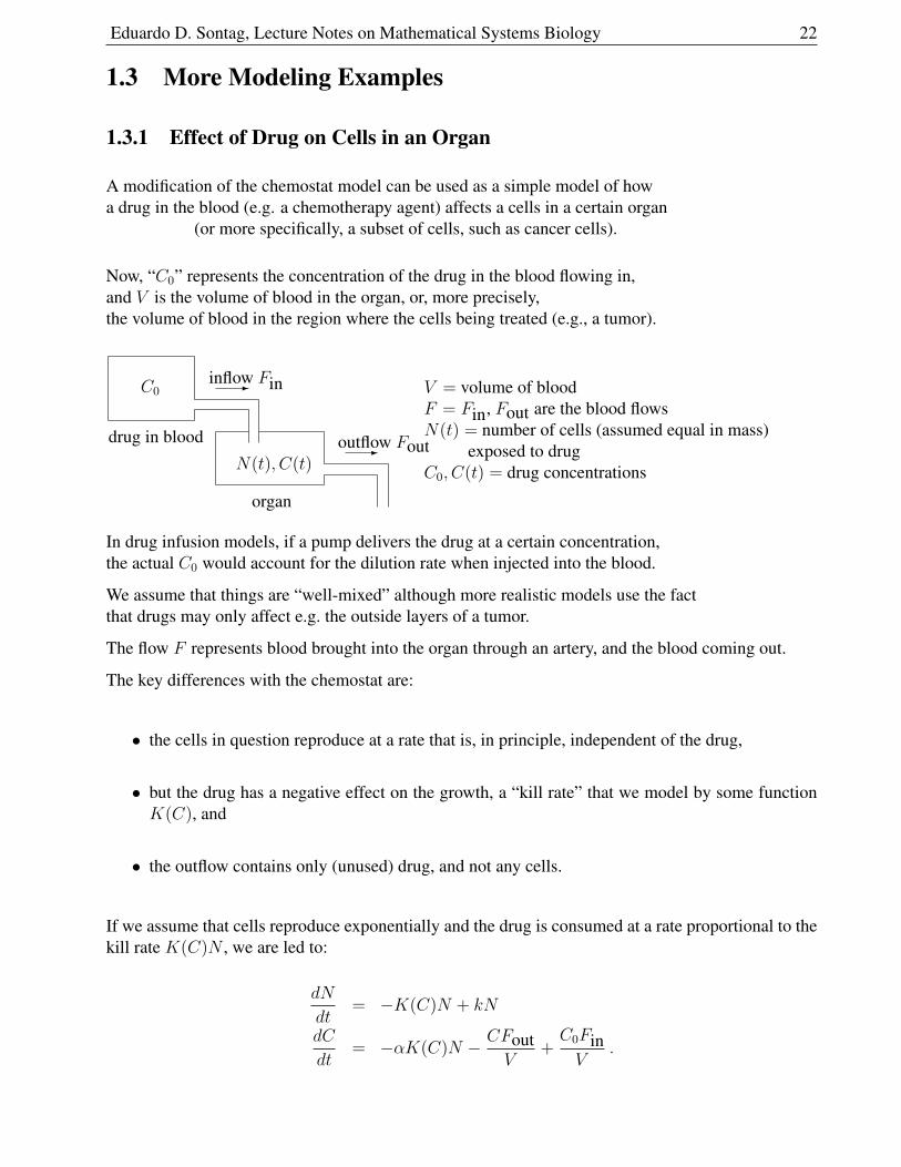
1.3.1 Effect of Drug on Cells in an Organ
A modification of the chemostat model can be used as a simple model of howa drug in the blood (e.g. a chemotherapy agent) affects a cells in a certain organ
(or more specifically, a subset of cells, such as cancer cells).
Now, “C0” represents the concentration of the drug in the blood flowing in,and V is the volume of blood in the organ, or, more precisely,the volume of blood in the region where the cells being treated (e.g., a tumor).
-
-drug in blood
organ
C0
N(t), C(t)
inflow Fin
outflow Fout
V = volume of bloodF = Fin, Fout are the blood flowsN(t) = number of cells (assumed equal in mass)
exposed to drugC0, C(t) = drug concentrations
In drug infusion models, if a pump delivers the drug at a certain concentration,the actual C0 would account for the dilution rate when injected into the blood.
We assume that things are “well-mixed” although more realistic models use the factthat drugs may only affect e.g. the outside layers of a tumor.
The flow F represents blood brought into the organ through an artery, and the blood coming out.
The key differences with the chemostat are:
• the cells in question reproduce at a rate that is, in principle, independent of the drug,
• but the drug has a negative effect on the growth, a “kill rate” that we model by some functionK(C), and
• the outflow contains only (unused) drug, and not any cells.
If we assume that cells reproduce exponentially and the drug is consumed at a rate proportional to thekill rate K(C)N , we are led to:
dN
dt= −K(C)N + kN
dC
dt= −αK(C)N − CFout
V+C0FinV
.
Eduardo D. Sontag, Lecture Notes on Mathematical Systems Biology 23
1.3.2 Compartmental Models
? ?
??
-
u2u1
d2d1
F21
F12
21
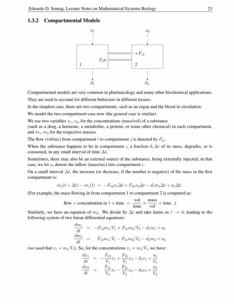
Compartmental models are very common in pharmacology and many other biochemical applications.
They are used to account for different behaviors in different tissues.
In the simplest case, there are two compartments, such as an organ and the blood in circulation.
We model the two-compartment case now (the general case is similar).
We use two variables x1, x2, for the concentrations (mass/vol) of a substance(such as a drug, a hormone, a metabolite, a protein, or some other chemical) in each compartment,and m1,m2 for the respective masses.
The flow (vol/sec) from compartment i to compartment j is denoted by Fij .
When the substance happens to be in compartment i, a fraction di ∆t of its mass, degrades, or isconsumed, in any small interval of time ∆t,
Sometimes, there may also be an external source of the substance, being externally injected; in thatcase, we let ui denote the inflow (mass/sec) into compartment i.
On a small interval ∆t, the increase (or decrease, if the number is negative) of the mass in the firstcompartment is:
m1(t+ ∆t)−m1(t) = −F12x1∆t+ F21x2∆t− d1m1∆t+ u1∆t .
(For example, the mass flowing in from compartment 1 to compartment 2 is computed as:
flow× concentration in 1× time =vol
time× mass
vol× time .)
Similarly, we have an equation of m2. We divide by ∆t and take limits as τ → 0, leading to thefollowing system of two linear differential equations:
dm1
dt= −F12m1/V1 + F21m2/V2 − d1m1 + u1
dm2
dt= F12m1/V1 − F21m2/V2 − d2m2 + u2
(we used that xi = mi/Vi). So, for the concentrations xi = mi/Vi, we have:
dx1
dt= −F12
V1
x1 +F21
V1
x2 − d1x1 +u1
V1
dx2
dt=
F12
V2
x1 −F21
V2
x2 − d2x2 +u2
V2
Eduardo D. Sontag, Lecture Notes on Mathematical Systems Biology 24
1.4 Geometric Analysis: Vector Fields, Phase Planes
1.4.1 Review: Vector Fields
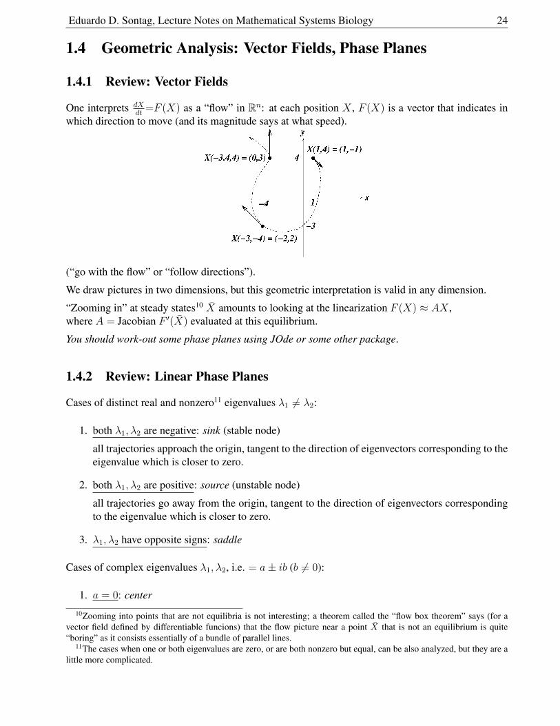
One interprets dXdt
=F (X) as a “flow” in Rn: at each position X , F (X) is a vector that indicates inwhich direction to move (and its magnitude says at what speed).
(“go with the flow” or “follow directions”).
We draw pictures in two dimensions, but this geometric interpretation is valid in any dimension.
“Zooming in” at steady states10 X amounts to looking at the linearization F (X) ≈ AX ,where A = Jacobian F ′(X) evaluated at this equilibrium.
You should work-out some phase planes using JOde or some other package.
1.4.2 Review: Linear Phase Planes
Cases of distinct real and nonzero11 eigenvalues λ1 6= λ2:
1. both λ1, λ2 are negative: sink (stable node)
all trajectories approach the origin, tangent to the direction of eigenvectors corresponding to theeigenvalue which is closer to zero.
2. both λ1, λ2 are positive: source (unstable node)
all trajectories go away from the origin, tangent to the direction of eigenvectors correspondingto the eigenvalue which is closer to zero.
3. λ1, λ2 have opposite signs: saddle
Cases of complex eigenvalues λ1, λ2, i.e. = a± ib (b 6= 0):
1. a = 0: center
10Zooming into points that are not equilibria is not interesting; a theorem called the “flow box theorem” says (for avector field defined by differentiable funcions) that the flow picture near a point X that is not an equilibrium is quite“boring” as it consists essentially of a bundle of parallel lines.
11The cases when one or both eigenvalues are zero, or are both nonzero but equal, can be also analyzed, but they are alittle more complicated.
Eduardo D. Sontag, Lecture Notes on Mathematical Systems Biology 25
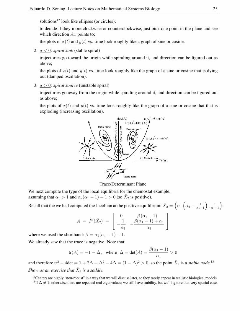
solutions12 look like ellipses (or circles);
to decide if they more clockwise or counterclockwise, just pick one point in the plane and seewhich direction Ax points to;
the plots of x(t) and y(t) vs. time look roughly like a graph of sine or cosine.
2. a < 0: spiral sink (stable spiral)
trajectories go toward the origin while spiraling around it, and direction can be figured out asabove;
the plots of x(t) and y(t) vs. time look roughly like the graph of a sine or cosine that is dyingout (damped oscillation).
3. a > 0: spiral source (unstable spiral)
trajectories go away from the origin while spiraling around it, and direction can be figured outas above;
the plots of x(t) and y(t) vs. time look roughly like the graph of a sine or cosine that that isexploding (increasing oscillation).
Trace/Determinant Plane
We next compute the type of the local equilibria for the chemostat example,assuming that α1 > 1 and α2(α1 − 1)− 1 > 0 (so X2 is positive).
Recall that the we had computed the Jacobian at the positive equilibrium X2 =(α1
(α2 − 1
α1−1
), 1α1−1
):
A = F ′(X2) =
0 β (α1 − 1)
− 1
α1
−β(α1 − 1) + α1
α1
where we used the shorthand: β = α2(α1 − 1)− 1.
We already saw that the trace is negative. Note that:
tr(A) = −1−∆ , where ∆ = det(A) =β(α1 − 1)
α1
> 0
and therefore tr2 − 4det = 1 + 2∆ + ∆2 − 4∆ = (1−∆)2 > 0, so the point X2 is a stable node.13
Show as an exercise that X1 is a saddle.12Centers are highly “non-robust” in a way that we will discuss later, so they rarely appear in realistic biological models.13If ∆ 6= 1; otherwise there are repeated real eigenvalues; we still have stability, but we’ll ignore that very special case.
Eduardo D. Sontag, Lecture Notes on Mathematical Systems Biology 26
1.4.3 Nullclines
Linearization helps understand the “local” picture of flows.14
It is much harder to get global information, telling us how these local pictures fit together(“connecting the dots” so to speak).
One useful technique when drawing global pictures is that of nullclines.
The xi-nullcline (if the variables are called x1, x2, . . .) is the set where dxidt
= 0.This set may be the union of several curves and lines, or just one such curve.
The intersections between the nullclines are the steady states. This is because each nullcline is the setwhere dx1/dt = 0, dx2/dt = 0, . . ., so intersecting gives points at which all dxi/dt = 0, that is to sayF (X) = 0 which is the definition of steady states.
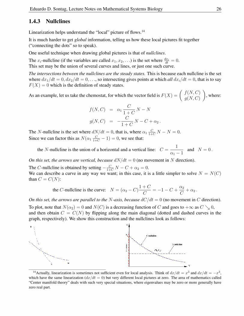
As an example, let us take the chemostat, for which the vector field is F (X) =
(f(N,C)g(N,C)
), where:
f(N,C) = α1C
1 + CN −N
g(N,C) = − C
1 + CN − C + α2 .
The N -nullcline is the set where dN/dt = 0, that is, where α1C
1+CN −N = 0.
Since we can factor this as N(α1C
1+C− 1) = 0, we see that:
the N -nullcline is the union of a horizontal and a vertical line: C =1
α1 − 1and N = 0 .
On this set, the arrows are vertical, because dN/dt = 0 (no movement in N direction).
The C-nullcline is obtained by setting − C1+C
N − C + α2 = 0.We can describe a curve in any way we want; in this case, it is a little simpler to solve N = N(C)than C = C(N):
the C-nullcline is the curve: N = (α2 − C)1 + C
C= −1− C +
α2
C+ α2 .
On this set, the arrows are parallel to the N -axis, because dC/dt = 0 (no movement in C direction).
To plot, note that N(α2) = 0 and N(C) is a decreasing function of C and goes to +∞ as C 0,and then obtain C = C(N) by flipping along the main diagonal (dotted and dashed curves in thegraph, respectively). We show this construction and the nullclines look as follows:
14Actually, linearization is sometimes not sufficient even for local analysis. Think of dx/dt = x3 and dx/dt = −x3,which have the same linearization (dx/dt = 0) but very different local pictures at zero. The area of mathematics called“Center manifold theory” deals with such very special situations, where eigenvalues may be zero or more generally havezero real part.
Eduardo D. Sontag, Lecture Notes on Mathematical Systems Biology 27
Assuming that α1 > 1 and α2 > 1/(α1 − 1), so that a positive steady-state exists, we have the twointersections: (0, α2) (saddle) and
(α1
(α2 − 1
α1−1
), 1α1−1
)(stable node).
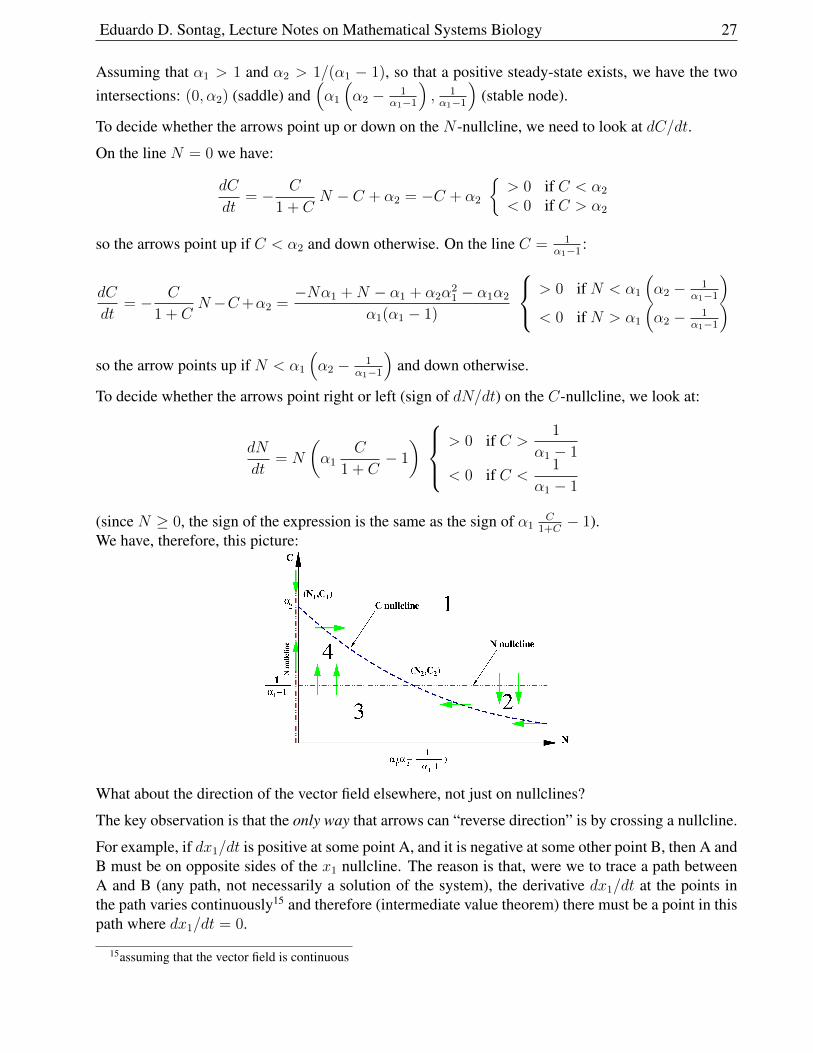
To decide whether the arrows point up or down on the N -nullcline, we need to look at dC/dt.
On the line N = 0 we have:
dC
dt= − C
1 + CN − C + α2 = −C + α2
> 0 if C < α2
< 0 if C > α2
so the arrows point up if C < α2 and down otherwise. On the line C = 1α1−1
:
dC
dt= − C
1 + CN−C+α2 =
−Nα1 +N − α1 + α2α21 − α1α2
α1(α1 − 1)
> 0 if N < α1
(α2 − 1
α1−1
)< 0 if N > α1
(α2 − 1
α1−1
)so the arrow points up if N < α1
(α2 − 1
α1−1
)and down otherwise.
To decide whether the arrows point right or left (sign of dN/dt) on the C-nullcline, we look at:
dN
dt= N
(α1
C
1 + C− 1
) > 0 if C >
1
α1 − 1
< 0 if C <1
α1 − 1
(since N ≥ 0, the sign of the expression is the same as the sign of α1C
1+C− 1).
We have, therefore, this picture:
What about the direction of the vector field elsewhere, not just on nullclines?
The key observation is that the only way that arrows can “reverse direction” is by crossing a nullcline.
For example, if dx1/dt is positive at some point A, and it is negative at some other point B, then A andB must be on opposite sides of the x1 nullcline. The reason is that, were we to trace a path betweenA and B (any path, not necessarily a solution of the system), the derivative dx1/dt at the points inthe path varies continuously15 and therefore (intermediate value theorem) there must be a point in thispath where dx1/dt = 0.
15assuming that the vector field is continuous
Eduardo D. Sontag, Lecture Notes on Mathematical Systems Biology 28
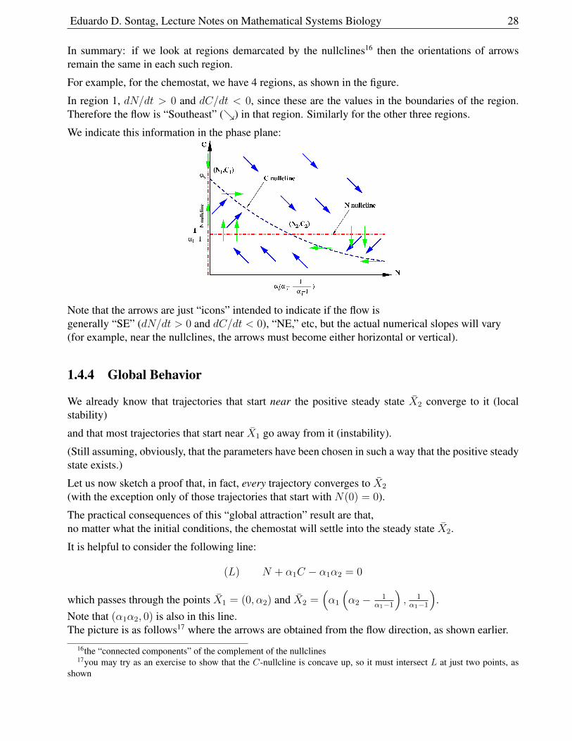
In summary: if we look at regions demarcated by the nullclines16 then the orientations of arrowsremain the same in each such region.
For example, for the chemostat, we have 4 regions, as shown in the figure.
In region 1, dN/dt > 0 and dC/dt < 0, since these are the values in the boundaries of the region.Therefore the flow is “Southeast” () in that region. Similarly for the other three regions.
We indicate this information in the phase plane:
Note that the arrows are just “icons” intended to indicate if the flow isgenerally “SE” (dN/dt > 0 and dC/dt < 0), “NE,” etc, but the actual numerical slopes will vary(for example, near the nullclines, the arrows must become either horizontal or vertical).
1.4.4 Global Behavior
We already know that trajectories that start near the positive steady state X2 converge to it (localstability)
and that most trajectories that start near X1 go away from it (instability).
(Still assuming, obviously, that the parameters have been chosen in such a way that the positive steadystate exists.)
Let us now sketch a proof that, in fact, every trajectory converges to X2
(with the exception only of those trajectories that start with N(0) = 0).
The practical consequences of this “global attraction” result are that,no matter what the initial conditions, the chemostat will settle into the steady state X2.
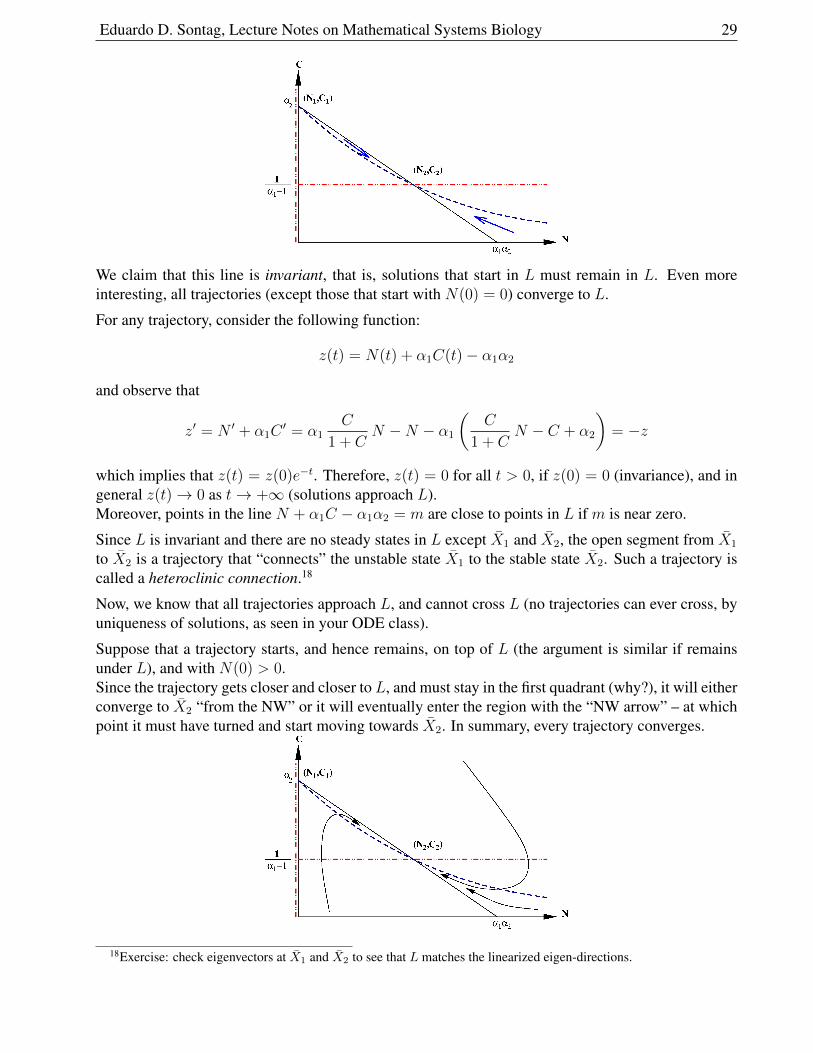
It is helpful to consider the following line:
(L) N + α1C − α1α2 = 0
which passes through the points X1 = (0, α2) and X2 =(α1
(α2 − 1
α1−1
), 1α1−1
).
Note that (α1α2, 0) is also in this line.The picture is as follows17 where the arrows are obtained from the flow direction, as shown earlier.
16the “connected components” of the complement of the nullclines17you may try as an exercise to show that the C-nullcline is concave up, so it must intersect L at just two points, as
shown
Eduardo D. Sontag, Lecture Notes on Mathematical Systems Biology 29
We claim that this line is invariant, that is, solutions that start in L must remain in L. Even moreinteresting, all trajectories (except those that start with N(0) = 0) converge to L.
For any trajectory, consider the following function:
z(t) = N(t) + α1C(t)− α1α2
and observe that
z′ = N ′ + α1C′ = α1
C
1 + CN −N − α1
(C
1 + CN − C + α2
)= −z
which implies that z(t) = z(0)e−t. Therefore, z(t) = 0 for all t > 0, if z(0) = 0 (invariance), and ingeneral z(t)→ 0 as t→ +∞ (solutions approach L).Moreover, points in the line N + α1C − α1α2 = m are close to points in L if m is near zero.
Since L is invariant and there are no steady states in L except X1 and X2, the open segment from X1
to X2 is a trajectory that “connects” the unstable state X1 to the stable state X2. Such a trajectory iscalled a heteroclinic connection.18
Now, we know that all trajectories approach L, and cannot cross L (no trajectories can ever cross, byuniqueness of solutions, as seen in your ODE class).
Suppose that a trajectory starts, and hence remains, on top of L (the argument is similar if remainsunder L), and with N(0) > 0.Since the trajectory gets closer and closer to L, and must stay in the first quadrant (why?), it will eitherconverge to X2 “from the NW” or it will eventually enter the region with the “NW arrow” – at whichpoint it must have turned and start moving towards X2. In summary, every trajectory converges.
18Exercise: check eigenvectors at X1 and X2 to see that L matches the linearized eigen-directions.
Eduardo D. Sontag, Lecture Notes on Mathematical Systems Biology 30
1.5 Epidemiology: SIRS Model
The modeling of infectious diseases and their spread is an important part of mathematical biology,part of the field of mathematical epidemiology.
Modeling is an important tool for gauging the impact of different vaccination programs on the controlor eradication of diseases.
We will only study here a simple ODE model, which does not take into account age structure norgeographical distribution. More sophisticated models can be based on compartmental systems, withcompartments corresponding to different age groups, partial differential equations, where independentvariables specify location, and so on, but the simple ODE model already brings up many of thefundamental ideas.
The classical work on epidemics dates back to Kermack and McKendrick, in 1927. We will studytheir SIR and SIRS models without “vital dynamics” (births and deaths).
To explain the model, let us think of a flu epidemic, but the ideas are very general.
In the population, there will be a group of people who are Susceptible to being passed on the virus bythe Infected individuals.
At some point, the infected individuals get so sick that they have to stay home, and become part ofthe Removed group. Once that they recover, they still cannot infect others, nor can they be infectedsince they developed immunity.
The numbers of individuals in the three classes will be denoted by S, I , and R respectively, and hencethe name “SIR” model.
Depending on the time-scale of interest for analysis, one may also allow for the fact that individualsin the Removed group may eventually return to the Susceptible population, which would happen ifimmunity is only temporary. This is the “SIRS” model (the last S to indicate flow from R to S),which we will study next.
We assume that these numbers are all functions of time t, and that the numbers can be modeled asreal numbers. (Non-integers make no sense for populations, but it is a mathematical convenience. Or,if one studies probabilistic instead of deterministic models, these numbers represent expected valuesof random variables, which can easily be non-integers.)
The basic modeling assumption is that the number of new infectives I(t+∆t)−I(t) in a small intervalof time [t, t+ ∆t] is proportional to the product S(t)I(t) ∆t.
Let us try to justify intuitively why it makes sense. (As usual, experimentation and fitting to datashould determine if this is a good assumption. In fact, alternative models have been proposed aswell.)
Suppose that transmission of the disease can happen only if a susceptible and infective are very closeto each other, for instance by direct contact, sneezing, etc.
We suppose that there is some region around a given susceptible individual, so that he can only getinfected if an infective enters that region:
We assume that, for each infective individual, there is a probability p = β∆t that this infective will
Eduardo D. Sontag, Lecture Notes on Mathematical Systems Biology 31
happen to pass through this region in the time interval [t, t + ∆t], where β is some positive constantthat depends on the size of the region, how fast the infectives are moving, etc. (Think of the infectivetraveling at a fixed speed: in twice the length of time, there is twice the chance that it will pass by thisregion.) We take ∆t 0, so also p 0.
The probability that this particular infective will not enter the region is 1− p, and, assuming indepen-dence, the probability than no infective enters is (1− p)I .
So the probability that some infective comes close to our susceptible is, using a binomial expansion:1− (1− p)I ≈ 1− (1− pI +
(I2
)p2 + . . .) ≈ pI since p 1.
Thus, we can say that a particular susceptible has a probability pI of being infected. Since there areS of them, we may assume, if S is large, that the total number infected will be S × pI .
We conclude that the number of new infections is:
I(t+ ∆t)− I(t) = pSI = βSI ∆t
and dividing by ∆t and taking limits, we have a term βSI in dIdt
, and similarly a term −βSI in dSdt
.
This is called a mass action kinetics assumption, and is also used when writing elementary chemicalreactions. In chemical reaction theory, one derives this mass action formula using “collision theory”among particles (for instance, molecules), taking into account temperature (which affects how fastparticles are moving), shapes, etc.
We also have to model infectives being removed: it is reasonable to assume that a certain fraction ofthem is removed per unit of time, giving terms νI , for some constant ν.
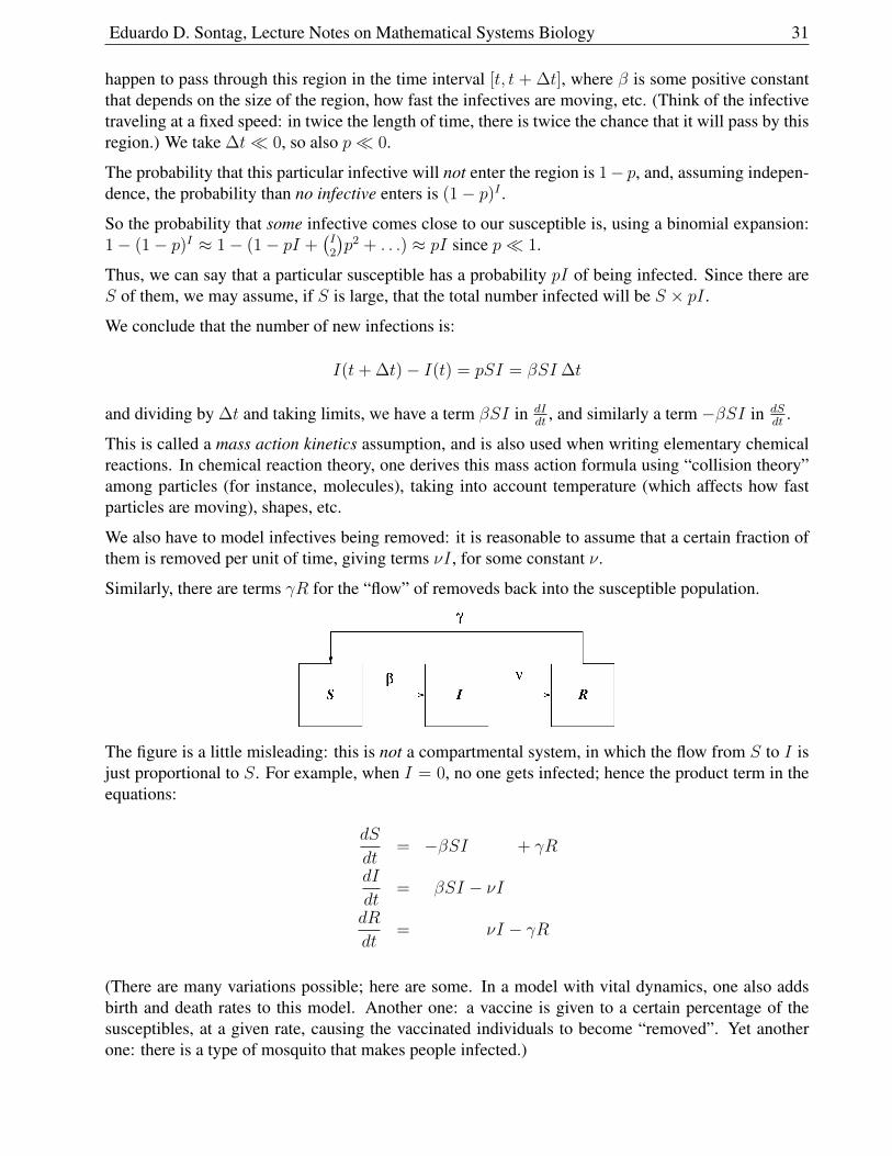
Similarly, there are terms γR for the “flow” of removeds back into the susceptible population.
The figure is a little misleading: this is not a compartmental system, in which the flow from S to I isjust proportional to S. For example, when I = 0, no one gets infected; hence the product term in theequations:
dS
dt= −βSI + γR
dI
dt= βSI − νI
dR
dt= νI − γR
(There are many variations possible; here are some. In a model with vital dynamics, one also addsbirth and death rates to this model. Another one: a vaccine is given to a certain percentage of thesusceptibles, at a given rate, causing the vaccinated individuals to become “removed”. Yet anotherone: there is a type of mosquito that makes people infected.)
Eduardo D. Sontag, Lecture Notes on Mathematical Systems Biology 32
1.5.1 Analysis of Equations
Let N = S(t) + I(t) +R(t). Since dN/dt = 0, N is constant, the total size of the population.
Therefore, even though we are interested in a system of three equations, this conservation law allowsus to eliminate one equation, for example, using R = N − S − I .
We are led to the study of the following two dimensional system:
dS
dt= −βSI + γ(N − S − I)
dI
dt= βSI − νI
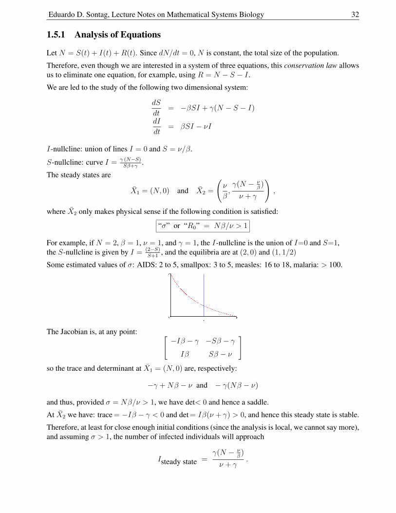
I-nullcline: union of lines I = 0 and S = ν/β.
S-nullcline: curve I = γ (N−S)Sβ+γ
.
The steady states are
X1 = (N, 0) and X2 =
(ν
β,γ(N − ν
β)
ν + γ
),
where X2 only makes physical sense if the following condition is satisfied:
“σ” or “R0” = Nβ/ν > 1
For example, if N = 2, β = 1, ν = 1, and γ = 1, the I-nullcline is the union of I=0 and S=1,the S-nullcline is given by I = (2−S)
S+1, and the equilibria are at (2, 0) and (1, 1/2)
Some estimated values of σ: AIDS: 2 to 5, smallpox: 3 to 5, measles: 16 to 18, malaria: > 100.
The Jacobian is, at any point: [−Iβ − γ −Sβ − γ
Iβ Sβ − ν
]so the trace and determinant at X1 = (N, 0) are, respectively:
−γ +Nβ − ν and − γ(Nβ − ν)
and thus, provided σ = Nβ/ν > 1, we have det< 0 and hence a saddle.
At X2 we have: trace = −Iβ − γ < 0 and det = Iβ(ν + γ) > 0, and hence this steady state is stable.
Therefore, at least for close enough initial conditions (since the analysis is local, we cannot say more),and assuming σ > 1, the number of infected individuals will approach
Isteady state =γ(N − ν
β)
ν + γ.
Eduardo D. Sontag, Lecture Notes on Mathematical Systems Biology 33
1.5.2 Interpreting σ
Let us give an intuitive interpretation of σ.
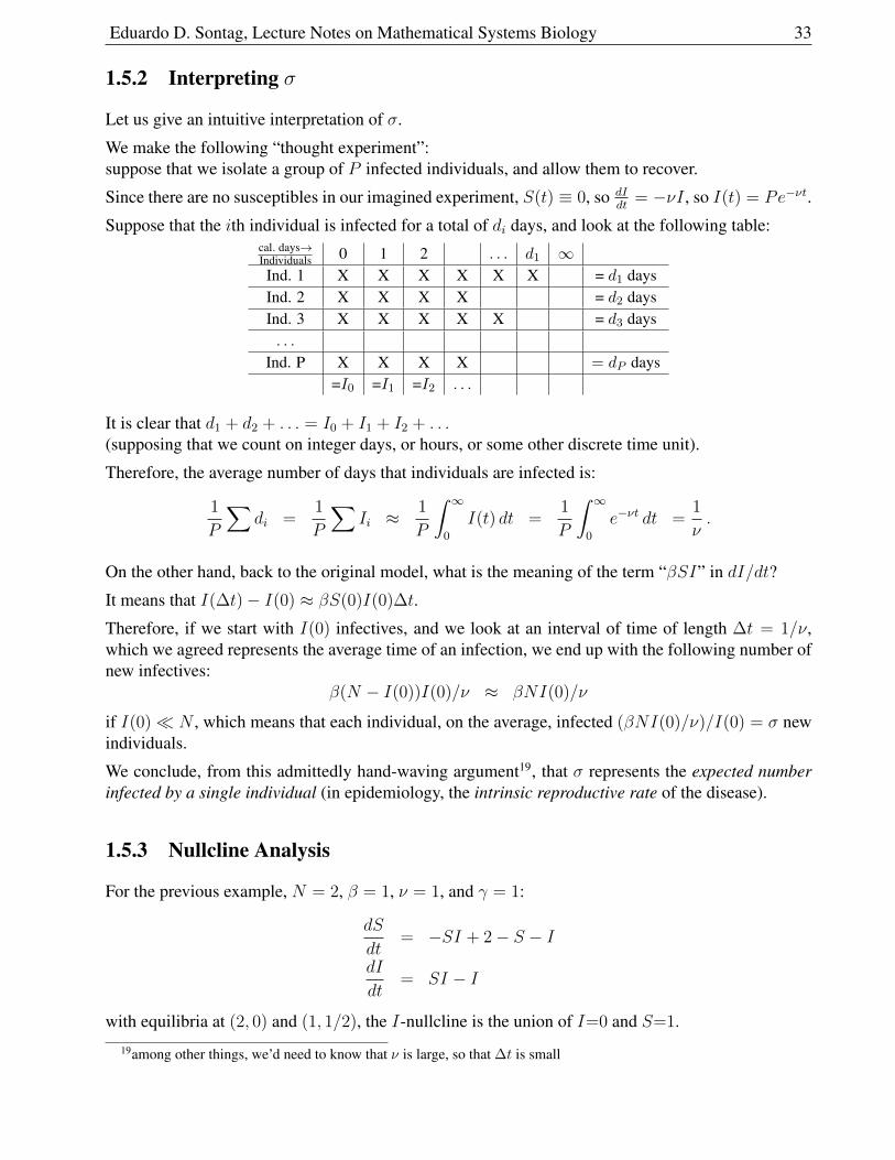
We make the following “thought experiment”:suppose that we isolate a group of P infected individuals, and allow them to recover.
Since there are no susceptibles in our imagined experiment, S(t) ≡ 0, so dIdt
= −νI , so I(t) = Pe−νt.
Suppose that the ith individual is infected for a total of di days, and look at the following table:cal. days→Individuals 0 1 2 . . . d1 ∞Ind. 1 X X X X X X = d1 daysInd. 2 X X X X = d2 daysInd. 3 X X X X X = d3 days. . .
Ind. P X X X X = dP days=I0 =I1 =I2 . . .
It is clear that d1 + d2 + . . . = I0 + I1 + I2 + . . .(supposing that we count on integer days, or hours, or some other discrete time unit).
Therefore, the average number of days that individuals are infected is:
1
P
∑di =
1
P
∑Ii ≈
1
P
∫ ∞0
I(t) dt =1
P
∫ ∞0
e−νt dt =1
ν.
On the other hand, back to the original model, what is the meaning of the term “βSI” in dI/dt?
It means that I(∆t)− I(0) ≈ βS(0)I(0)∆t.
Therefore, if we start with I(0) infectives, and we look at an interval of time of length ∆t = 1/ν,which we agreed represents the average time of an infection, we end up with the following number ofnew infectives:
β(N − I(0))I(0)/ν ≈ βNI(0)/ν
if I(0) N , which means that each individual, on the average, infected (βNI(0)/ν)/I(0) = σ newindividuals.
We conclude, from this admittedly hand-waving argument19, that σ represents the expected numberinfected by a single individual (in epidemiology, the intrinsic reproductive rate of the disease).
1.5.3 Nullcline Analysis
For the previous example, N = 2, β = 1, ν = 1, and γ = 1:
dS
dt= −SI + 2− S − I
dI
dt= SI − I
with equilibria at (2, 0) and (1, 1/2), the I-nullcline is the union of I=0 and S=1.
19among other things, we’d need to know that ν is large, so that ∆t is small
Eduardo D. Sontag, Lecture Notes on Mathematical Systems Biology 34
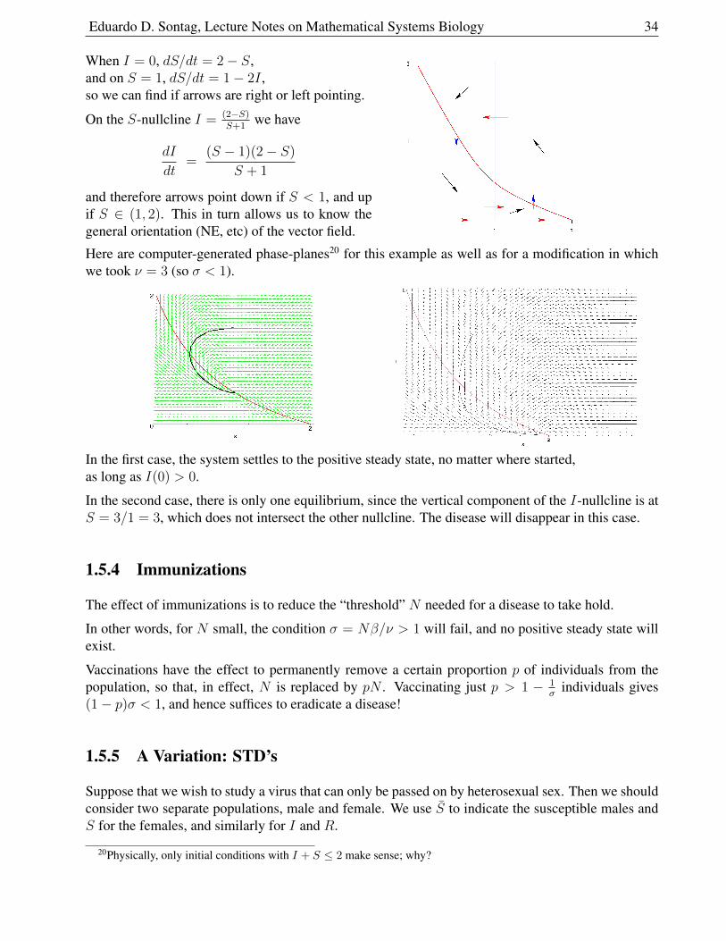
When I = 0, dS/dt = 2− S,and on S = 1, dS/dt = 1− 2I ,so we can find if arrows are right or left pointing.
On the S-nullcline I = (2−S)S+1
we have
dI
dt=
(S − 1)(2− S)
S + 1
and therefore arrows point down if S < 1, and upif S ∈ (1, 2). This in turn allows us to know thegeneral orientation (NE, etc) of the vector field.
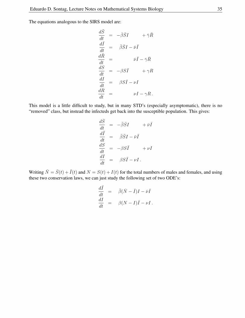
Here are computer-generated phase-planes20 for this example as well as for a modification in whichwe took ν = 3 (so σ < 1).
In the first case, the system settles to the positive steady state, no matter where started,as long as I(0) > 0.
In the second case, there is only one equilibrium, since the vertical component of the I-nullcline is atS = 3/1 = 3, which does not intersect the other nullcline. The disease will disappear in this case.
1.5.4 Immunizations
The effect of immunizations is to reduce the “threshold” N needed for a disease to take hold.
In other words, for N small, the condition σ = Nβ/ν > 1 will fail, and no positive steady state willexist.
Vaccinations have the effect to permanently remove a certain proportion p of individuals from thepopulation, so that, in effect, N is replaced by pN . Vaccinating just p > 1 − 1
σindividuals gives
(1− p)σ < 1, and hence suffices to eradicate a disease!
1.5.5 A Variation: STD’s
Suppose that we wish to study a virus that can only be passed on by heterosexual sex. Then we shouldconsider two separate populations, male and female. We use S to indicate the susceptible males andS for the females, and similarly for I and R.
20Physically, only initial conditions with I + S ≤ 2 make sense; why?
Eduardo D. Sontag, Lecture Notes on Mathematical Systems Biology 35
The equations analogous to the SIRS model are:
dS
dt= −βSI + γR
dI
dt= βSI − νI
dR
dt= νI − γR
dS
dt= −βSI + γR
dI
dt= βSI − νI
dR
dt= νI − γR .
This model is a little difficult to study, but in many STD’s (especially asymptomatic), there is no“removed” class, but instead the infecteds get back into the susceptible population. This gives:
dS
dt= −βSI + νI
dI
dt= βSI − νI
dS
dt= −βSI + νI
dI
dt= βSI − νI .
Writing N = S(t) + I(t) and N = S(t) + I(t) for the total numbers of males and females, and usingthese two conservation laws, we can just study the following set of two ODE’s:
dI
dt= β(N − I)I − νI
dI
dt= β(N − I)I − νI .
Eduardo D. Sontag, Lecture Notes on Mathematical Systems Biology 36
1.6 Chemical Kinetics
Elementary reactions (in a gas or liquid) are due to collisions of particles (molecules, atoms).
Particles move at a velocity that depends on temperature (higher temperature⇒ faster).
The law of mass action is:
reaction rates (at constant temperature) are proportional to products of concentrations.
This law may be justified intuitively in various ways, for instance, using an argument like the one thatwe presented for disease transmission.
In chemistry, collision theory studies this question and justifies mass-action kinetics.
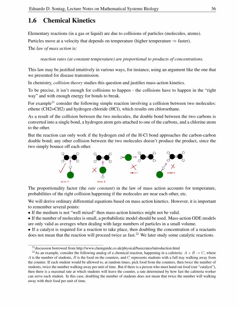
To be precise, it isn’t enough for collisions to happen - the collisions have to happen in the “rightway” and with enough energy for bonds to break.
For example21 consider the following simple reaction involving a collision between two molecules:ethene (CH2=CH2) and hydrogen chloride (HCl), which results om chloroethane.
As a result of the collision between the two molecules, the double bond between the two carbons isconverted into a single bond, a hydrogen atom gets attached to one of the carbons, and a chlorine atomto the other.
But the reaction can only work if the hydrogen end of the H-Cl bond approaches the carbon-carbondouble bond; any other collision between the two molecules doesn’t produce the product, since thetwo simply bounce off each other.
The proportionality factor (the rate constant) in the law of mass action accounts for temperature,probabilities of the right collision happening if the molecules are near each other, etc.
We will derive ordinary differential equations based on mass action kinetics. However, it is importantto remember several points:• If the medium is not “well mixed” then mass-action kinetics might not be valid.• If the number of molecules is small, a probabilistic model should be used. Mass-action ODE modelsare only valid as averages when dealing with large numbers of particles in a small volume.• If a catalyst is required for a reaction to take place, then doubling the concentration of a reactantsdoes not mean that the reaction will proceed twice as fast.22 We later study some catalytic reactions.
21discussion borrowed from http://www.chemguide.co.uk/physical/basicrates/introduction.html22As an example, consider the following analog of a chemical reaction, happening in a cafeteria: A + B → C, where
A is the number of students, B is the food on the counters, and C represents students with a full tray walking away fromthe counter. If each student would be allowed to, at random times, pick food from the counters, then twice the number ofstudents, twice the number walking away per unit of time. But if there is a person who must hand out food (our “catalyst”),then there is a maximal rate at which students will leave the counter, a rate determined by how fast the cafeteria workercan serve each student. In this case, doubling the number of students does not mean that twice the number will walkingaway with their food per unit of time.
Eduardo D. Sontag, Lecture Notes on Mathematical Systems Biology 37
1.6.1 Equations
We will use capital letters A,B, . . . for names of chemical substances (molecules, ions, etc), andlower-case a, b, . . . for their corresponding concentrations.
There is a systematic way to write down equations for chemical reactions, using a graph descriptionof the reactions and formulas for the different kinetic terms. We discuss this systematic approachlater, but for now we consider some very simple reactions, for which we can write equations directly.We simply use the mass-action principle for each separate reaction, and add up all the effects.
The simplest “reaction” is one where there is only one reactant, that can degrade23 or decay (as inradioactive decay), or be transformed into another species, or split into several constituents.
In either case, the rate of the reaction is proportional to the concentration:if we have twice the amount of substance X in a certain volume, then, per (small) unit of time, acertain % of the substance in this volume will disappear, which means that the concentration willdiminish by that fraction.A corresponding number of the new substances is then produced, per unit of time.
So, decay X k−→ · gives the ODE:dx/dt = −kx ,
a transformation X k−→ Y gives:
dx/dt = −kxdy/dt = kx ,
and a dissociation reaction Z k−→ X + Y gives:
dx/dt = kz
dy/dt = kz
dz/dt = −kz .
A bimolecular reaction X + Yk+−→ Z gives:
dx/dt = −k+xy
dy/dt = −k+xy
dz/dt = k+xy
and if the reverse reaction Zk−−→ X + Y also takes place:
x = −k+xy + k−z
y = −k+xy + k−z
z = k+xy − k−z .23Of course, “degrade” is a relative concept, because the separate parts of the decaying substance should be taken
account of. However, if these parts are not active in any further reactions, one ignores them and simply thinks of thereactant as disappearing!
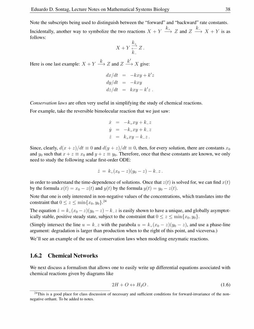
Eduardo D. Sontag, Lecture Notes on Mathematical Systems Biology 38
Note the subscripts being used to distinguish between the “forward” and “backward” rate constants.
Incidentally, another way to symbolize the two reactions X + Yk+−→ Z and Z
k−−→ X + Y is asfollows:
X + Yk+−→←−k−
Z .
Here is one last example: X + Yk−→ Z and Z k′−→ X give:
dx/dt = −kxy + k′z
dy/dt = −kxydz/dt = kxy − k′z .
Conservation laws are often very useful in simplifying the study of chemical reactions.
For example, take the reversible bimolecular reaction that we just saw:
x = −k+xy + k−z
y = −k+xy + k−z
z = k+xy − k−z .
Since, clearly, d(x + z)/dt ≡ 0 and d(y + z)/dt ≡ 0, then, for every solution, there are constants x0
and y0 such that x+ z ≡ x0 and y+ z ≡ y0. Therefore, once that these constants are known, we onlyneed to study the following scalar first-order ODE:
z = k+(x0 − z)(y0 − z)− k−z .
in order to understand the time-dependence of solutions. Once that z(t) is solved for, we can find x(t)by the formula x(t) = x0 − z(t) and y(t) by the formula y(t) = y0 − z(t).
Note that one is only interested in non-negative values of the concentrations, which translates into theconstraint that 0 ≤ z ≤ minx0, y0.24
The equation z = k+(x0− z)(y0− z)− k−z is easily shown to have a unique, and globally asymptot-ically stable, positive steady state, subject to the constraint that 0 ≤ z ≤ minx0, y0.(Simply intersect the line u = k−z with the parabola u = k+(x0 − z)(y0 − z), and use a phase-lineargument: degradation is larger than production when to the right of this point, and viceversa.)
We’ll see an example of the use of conservation laws when modeling enzymatic reactions.
1.6.2 Chemical Networks
We next discuss a formalism that allows one to easily write up differential equations associated withchemical reactions given by diagrams like
2H +O ↔ H2O . (1.6)
24This is a good place for class discussion of necessary and sufficient conditions for forward-invariance of the non-negative orthant. To be added to notes.

Eduardo D. Sontag, Lecture Notes on Mathematical Systems Biology 39
In general, we consider a collection of chemical reactions that involves a set of ns “species”:
Si, i ∈ 1, 2, . . . ns .
These “species” may be ions, atoms, or molecules (even large molecules, such as proteins). We’ll justsay “molecules”, for simplicity. For example, (1.6) represents a set of two reactions that involve thefollowing ns = 3 species (hydrogen, oxygen, water):
S1 = H, S2 = O, S3 = H2O ,
one going forward and one going backward. In general, a chemical reaction network (“CRN”, forshort) is a set of chemical reactionsRj , j ∈ 1, 2, . . . , nr:
Rj :ns∑i=1
αijSi →ns∑i=1
βijSi (1.7)
where the αij and βij are some nonnegative integers, called the stoichiometry coefficients.
The species with nonzero coefficients on the left-hand side are usually referred to as the reactants, andthe ones on the right-hand side are called the products, of the respective reaction. (Zero coefficients arenot shown in diagrams.) The interpretation is that, in reaction 1, α11 molecules of species S1 combinewith α21 molecules of species S2, etc., to produce β11 molecules of species S1, β21 molecules ofspecies S2, etc., and similarly for each of the other nr − 1 reactions.
The forward arrow means that the transformation of reactants into products only happens in the di-rection of the arrow. For example, the reversible reaction (1.6) is represented by the following CRN,with nr = 2 reactions:
R1 : 2H +O → H2O
R2 : H2O → 2H +O .
So, in this example,
α11 = 2, α21 = 1, α31 = 0, β11 = 0, β21 = 0, β31 = 1,
andα12 = 0, α22 = 0, α32 = 1, β12 = 2, β22 = 1, β32 = 0 .
It is convenient to arrange the stoichiometry coefficients into an ns × nr matrix, called the stoichiom-etry matrix Γ = Γij , defined as follows:
Γij = βij − αij , i = 1, . . . , ns , j = 1, . . . , nr . (1.8)
The matrix Γ has as many columns as there are reactions. Each column shows, for all species (orderedaccording to their index i), the net “produced−consumed”. For example, for the reaction (1.6), Γ isthe following matrix: −2 2
−1 11 −1
.
Notice that we allow degradation reactions like A→ 0 (all β’s are zero for this reaction).
Eduardo D. Sontag, Lecture Notes on Mathematical Systems Biology 40
We now describe how the state of the network evolves over time, for a given CRN. We need to find arule for the evolution of the vector:
[S1(t)][S2(t)]
...[Sns(t)]
where the notation [Si(t)] means the concentration of the species Si at time t. For simplicity, we dropthe brackets and write Si also for the concentration of Si (sometimes, to avoid confusion, we useinstead lower-case letters like si to denote concentrations). As usual with differential equations, wealso drop the argument “t” if it is clear from the context. Observe that only nonnegative concentrationsmake physical sense (a zero concentration means that a species is not present at all).
The graphical information given by reaction diagrams is summarized by the matrix Γ. Another ingre-dient that we require is a formula for the actual rate at which the individual reactions take place.
We denote by Rj(S) be algebraic form of the jth reaction. The most common assumption is that ofmass-action kinetics, where:
Rj(S) = kj
ns∏i=1
Sαiji for all j = 1, . . . , nr .
This says simply that the reaction rate is proportional to the products of concentrations of the reactants,with higher exponents when more than one molecule is needed. The coefficients ki are “reactionconstants” which usually label the arrows in diagrams. Let us write the vector of reactions as R(S):
R(S) :=
R1(S)R2(S)
...Rnr(S)
.
With these conventions, the system of differential equations associated to the CRN is given as follows:
dS
dt= ΓR(S) . (1.9)
Example
As an illustrative example, let us consider the following set of chemical reactions:
E + Pk1−→←−k−1
Ck2−→ E +Q, F +Q
k3−→←−k−3
Dk4−→ F + P, (1.10)
which may be thought of as a model of the activation (for instance, by phosphorylation) of a proteinsubstrate P by an enzyme E; C is an intermediate complex, which dissociates either back into theoriginal components or into a product (activated protein) Q and the enzyme. The second reactiontransforms Q back into P , and is catalyzed by another enzyme F (for instance, a phosphatase thatremoves the phosphorylation). A system of reactions of this type is sometimes called a “futile cycle”,and reactions of this type are ubiquitous in cell biology. The mass-action kinetics model is then
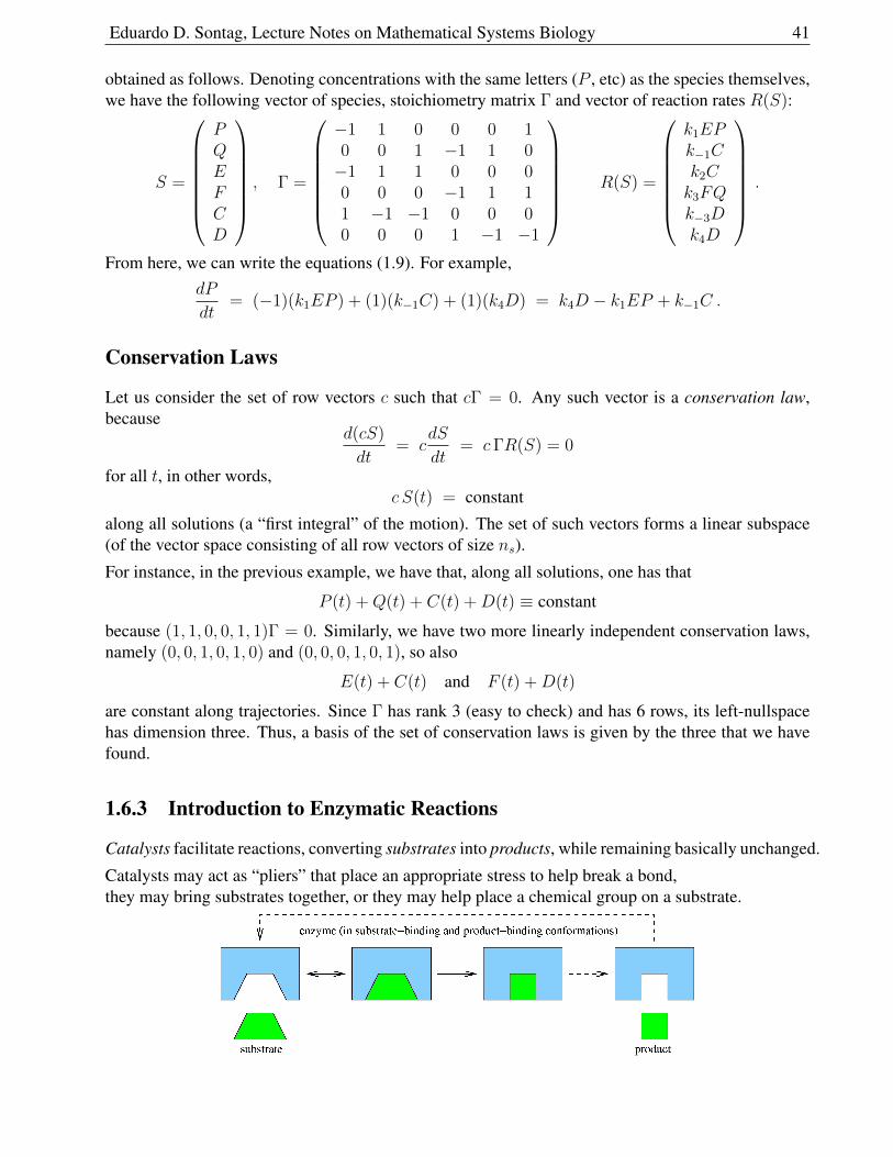
Eduardo D. Sontag, Lecture Notes on Mathematical Systems Biology 41
obtained as follows. Denoting concentrations with the same letters (P , etc) as the species themselves,we have the following vector of species, stoichiometry matrix Γ and vector of reaction rates R(S):
S =
PQEFCD
, Γ =
−1 1 0 0 0 10 0 1 −1 1 0−1 1 1 0 0 00 0 0 −1 1 11 −1 −1 0 0 00 0 0 1 −1 −1
R(S) =
k1EPk−1Ck2Ck3FQk−3Dk4D
.
From here, we can write the equations (1.9). For example,dP
dt= (−1)(k1EP ) + (1)(k−1C) + (1)(k4D) = k4D − k1EP + k−1C .
Conservation Laws
Let us consider the set of row vectors c such that cΓ = 0. Any such vector is a conservation law,because
d(cS)
dt= c
dS
dt= cΓR(S) = 0
for all t, in other words,c S(t) = constant
along all solutions (a “first integral” of the motion). The set of such vectors forms a linear subspace(of the vector space consisting of all row vectors of size ns).
For instance, in the previous example, we have that, along all solutions, one has that
P (t) +Q(t) + C(t) +D(t) ≡ constant
because (1, 1, 0, 0, 1, 1)Γ = 0. Similarly, we have two more linearly independent conservation laws,namely (0, 0, 1, 0, 1, 0) and (0, 0, 0, 1, 0, 1), so also
E(t) + C(t) and F (t) +D(t)
are constant along trajectories. Since Γ has rank 3 (easy to check) and has 6 rows, its left-nullspacehas dimension three. Thus, a basis of the set of conservation laws is given by the three that we havefound.
1.6.3 Introduction to Enzymatic Reactions
Catalysts facilitate reactions, converting substrates into products, while remaining basically unchanged.
Catalysts may act as “pliers” that place an appropriate stress to help break a bond,they may bring substrates together, or they may help place a chemical group on a substrate.
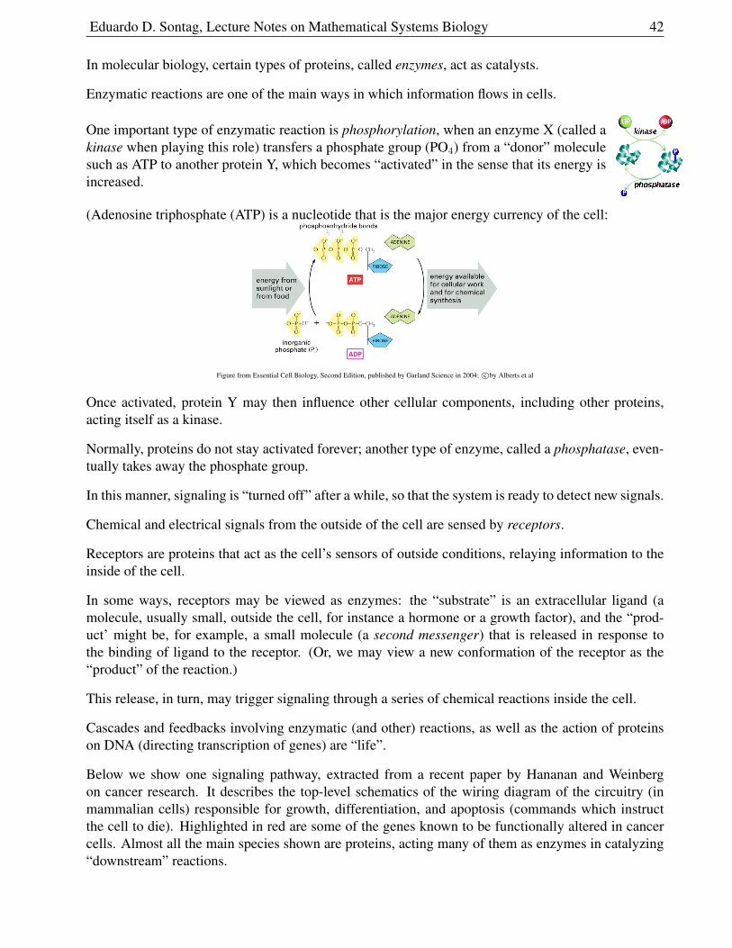
Eduardo D. Sontag, Lecture Notes on Mathematical Systems Biology 42
In molecular biology, certain types of proteins, called enzymes, act as catalysts.
Enzymatic reactions are one of the main ways in which information flows in cells.
One important type of enzymatic reaction is phosphorylation, when an enzyme X (called akinase when playing this role) transfers a phosphate group (PO4) from a “donor” moleculesuch as ATP to another protein Y, which becomes “activated” in the sense that its energy isincreased.
(Adenosine triphosphate (ATP) is a nucleotide that is the major energy currency of the cell:
Figure from Essential Cell Biology, Second Edition, published by Garland Science in 2004; c©by Alberts et al
Once activated, protein Y may then influence other cellular components, including other proteins,acting itself as a kinase.
Normally, proteins do not stay activated forever; another type of enzyme, called a phosphatase, even-tually takes away the phosphate group.
In this manner, signaling is “turned off” after a while, so that the system is ready to detect new signals.
Chemical and electrical signals from the outside of the cell are sensed by receptors.
Receptors are proteins that act as the cell’s sensors of outside conditions, relaying information to theinside of the cell.
In some ways, receptors may be viewed as enzymes: the “substrate” is an extracellular ligand (amolecule, usually small, outside the cell, for instance a hormone or a growth factor), and the “prod-uct’ might be, for example, a small molecule (a second messenger) that is released in response tothe binding of ligand to the receptor. (Or, we may view a new conformation of the receptor as the“product” of the reaction.)
This release, in turn, may trigger signaling through a series of chemical reactions inside the cell.
Cascades and feedbacks involving enzymatic (and other) reactions, as well as the action of proteinson DNA (directing transcription of genes) are “life”.
Below we show one signaling pathway, extracted from a recent paper by Hananan and Weinbergon cancer research. It describes the top-level schematics of the wiring diagram of the circuitry (inmammalian cells) responsible for growth, differentiation, and apoptosis (commands which instructthe cell to die). Highlighted in red are some of the genes known to be functionally altered in cancercells. Almost all the main species shown are proteins, acting many of them as enzymes in catalyzing“downstream” reactions.
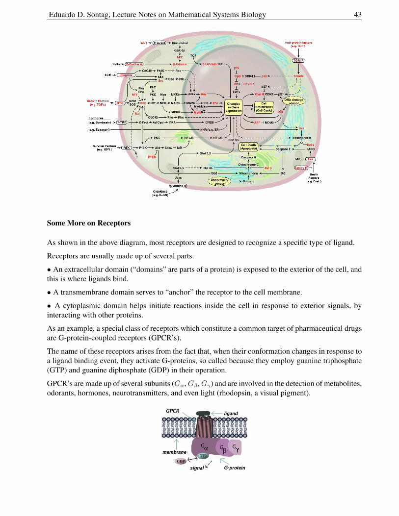
Eduardo D. Sontag, Lecture Notes on Mathematical Systems Biology 43
Some More on Receptors
As shown in the above diagram, most receptors are designed to recognize a specific type of ligand.
Receptors are usually made up of several parts.
• An extracellular domain (“domains” are parts of a protein) is exposed to the exterior of the cell, andthis is where ligands bind.
• A transmembrane domain serves to “anchor” the receptor to the cell membrane.
• A cytoplasmic domain helps initiate reactions inside the cell in response to exterior signals, byinteracting with other proteins.
As an example, a special class of receptors which constitute a common target of pharmaceutical drugsare G-protein-coupled receptors (GPCR’s).
The name of these receptors arises from the fact that, when their conformation changes in response toa ligand binding event, they activate G-proteins, so called because they employ guanine triphosphate(GTP) and guanine diphosphate (GDP) in their operation.
GPCR’s are made up of several subunits (Gα,Gβ ,Gγ) and are involved in the detection of metabolites,odorants, hormones, neurotransmitters, and even light (rhodopsin, a visual pigment).
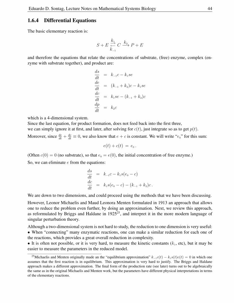
Eduardo D. Sontag, Lecture Notes on Mathematical Systems Biology 44
1.6.4 Differential Equations
The basic elementary reaction is:
S + Ek1−→←−k−1
Ck2−→ P + E
and therefore the equations that relate the concentrations of substrate, (free) enzyme, complex (en-zyme with substrate together), and product are:
ds
dt= k−1c− k1se
de
dt= (k−1 + k2)c− k1se
dc
dt= k1se− (k−1 + k2)c
dp
dt= k2c
which is a 4-dimensional system.Since the last equation, for product formation, does not feed back into the first three,we can simply ignore it at first, and later, after solving for c(t), just integrate so as to get p(t).
Moreover, since dedt
+ dcdt≡ 0, we also know that e+ c is constant. We will write “e0” for this sum:
e(t) + c(t) = e0 .
(Often c(0) = 0 (no substrate), so that e0 = e(0), the initial concentration of free enzyme.)
So, we can eliminate e from the equations:
ds
dt= k−1c− k1s(e0 − c)
dc
dt= k1s(e0 − c)− (k−1 + k2)c .
We are down to two dimensions, and could proceed using the methods that we have been discussing.
However, Leonor Michaelis and Maud Leonora Menten formulated in 1913 an approach that allowsone to reduce the problem even further, by doing an approximation. Next, we review this approach,as reformulated by Briggs and Haldane in 192525, and interpret it in the more modern language ofsingular perturbation theory.
Although a two-dimensional system is not hard to study, the reduction to one dimension is very useful:• When “connecting” many enzymatic reactions, one can make a similar reduction for each one ofthe reactions, which provides a great overall reduction in complexity.• It is often not possible, or it is very hard, to measure the kinetic constants (k1, etc), but it may beeasier to measure the parameters in the reduced model.
25Michaelis and Menten originally made an the “equilibrium approximation” k−1c(t) − k1s(t)e(t) = 0 in which oneassumes that the first reaction is in equilibrium. This approximation is very hard to justify. The Briggs and Haldaneapproach makes a different approximation. The final form of the production rate (see later) turns out to be algebraicallythe same as in the original Michaelis and Menten work, but the parameters have different physical interpretations in termsof the elementary reactions.
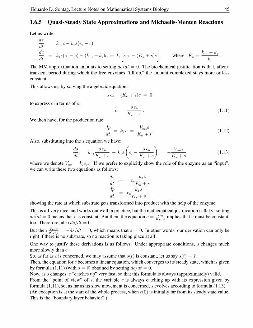
Eduardo D. Sontag, Lecture Notes on Mathematical Systems Biology 45
1.6.5 Quasi-Steady State Approximations and Michaelis-Menten Reactions
Let us writeds
dt= k−1c− k1s(e0 − c)
dc
dt= k1s(e0 − c)− (k−1 + k2)c = k1
[s e0 − (Km + s)c
], where Km =
k−1 + k2
k1
.
The MM approximation amounts to setting dc/dt = 0. The biochemical justification is that, after atransient period during which the free enzymes “fill up,” the amount complexed stays more or lessconstant.
This allows us, by solving the algebraic equation:
s e0 − (Km + s)c = 0
to express c in terms of s:c =
s e0Km + s
. (1.11)
We then have, for the production rate:dp
dt= k2 c =
Vmaxs
Km + s. (1.12)
Also, substituting into the s equation we have:
ds
dt= k−1
s e0Km + s
− k1s
(e0 −
s e0Km + s
)= − Vmaxs
Km + s(1.13)
where we denote Vmax = k2e0. If we prefer to explicitly show the role of the enzyme as an “input”,we can write these two equations as follows:
ds
dt= −e0
k2 s
Km + sdp
dt= e0
k2 s
Km + s
showing the rate at which substrate gets transformed into product with the help of the enzyme.
This is all very nice, and works out well in practice, but the mathematical justification is flaky: settingdc/dt = 0 means that c is constant. But then, the equation c = s e0
Km+simplies that s must be constant,
too. Therefore, also ds/dt = 0.
But then VmaxsKm+s
= −ds/dt = 0, which means that s = 0. In other words, our derivation can only beright if there is no substrate, so no reaction is taking place at all!
One way to justify these derivations is as follows. Under appropriate conditions, s changes muchmore slowly than c.So, as far as c is concerned, we may assume that s(t) is constant, let us say s(t) = s.Then, the equation for c becomes a linear equation, which converges to its steady state, which is givenby formula (1.11) (with s = s) obtained by setting dc/dt = 0.Now, as s changes, c “catches up” very fast, so that this formula is always (approximately) valid.From the “point of view” of s, the variable c is always catching up with its expression given byformula (1.11), so, as far as its slow movement is concerned, s evolves according to formula (1.13).(An exception is at the start of the whole process, when c(0) is initially far from its steady state value.This is the “boundary layer behavior”.)
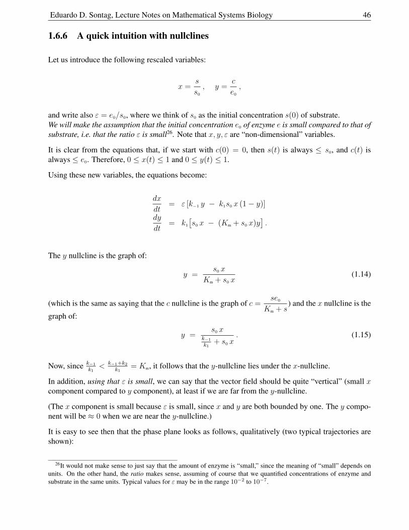
Eduardo D. Sontag, Lecture Notes on Mathematical Systems Biology 46
1.6.6 A quick intuition with nullclines
Let us introduce the following rescaled variables:
x =s
s0, y =
c
e0,
and write also ε = e0/s0, where we think of s0 as the initial concentration s(0) of substrate.We will make the assumption that the initial concentration e0 of enzyme e is small compared to that ofsubstrate, i.e. that the ratio ε is small26. Note that x, y, ε are “non-dimensional” variables.
It is clear from the equations that, if we start with c(0) = 0, then s(t) is always ≤ s0, and c(t) isalways ≤ e0. Therefore, 0 ≤ x(t) ≤ 1 and 0 ≤ y(t) ≤ 1.
Using these new variables, the equations become:
dx
dt= ε [k−1 y − k1s0 x (1− y)]
dy
dt= k1
[s0 x − (Km + s0 x)y
].
The y nullcline is the graph of:
y =s0 x
Km + s0 x(1.14)
(which is the same as saying that the c nullcline is the graph of c =se0
Km + s) and the x nullcline is the
graph of:
y =s0 x
k−1
k1+ s0 x
. (1.15)
Now, since k−1
k1< k−1+k2
k1= Km, it follows that the y-nullcline lies under the x-nullcline.
In addition, using that ε is small, we can say that the vector field should be quite “vertical” (small xcomponent compared to y component), at least if we are far from the y-nullcline.
(The x component is small because ε is small, since x and y are both bounded by one. The y compo-nent will be ≈ 0 when we are near the y-nullcline.)
It is easy to see then that the phase plane looks as follows, qualitatively (two typical trajectories areshown):
26It would not make sense to just say that the amount of enzyme is “small,” since the meaning of “small” depends onunits. On the other hand, the ratio makes sense, assuming of course that we quantified concentrations of enzyme andsubstrate in the same units. Typical values for ε may be in the range 10−2 to 10−7.
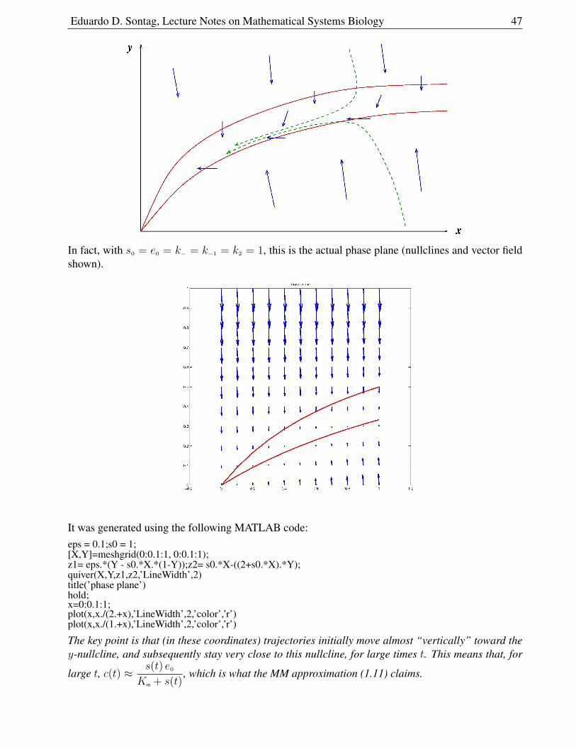
Eduardo D. Sontag, Lecture Notes on Mathematical Systems Biology 47
In fact, with s0 = e0 = k− = k−1 = k2 = 1, this is the actual phase plane (nullclines and vector fieldshown).
It was generated using the following MATLAB code:eps = 0.1;s0 = 1;[X,Y]=meshgrid(0:0.1:1, 0:0.1:1);z1= eps.*(Y - s0.*X.*(1-Y));z2= s0.*X-((2+s0.*X).*Y);quiver(X,Y,z1,z2,’LineWidth’,2)title(’phase plane’)hold;x=0:0.1:1;plot(x,x./(2.+x),’LineWidth’,2,’color’,’r’)plot(x,x./(1.+x),’LineWidth’,2,’color’,’r’)
The key point is that (in these coordinates) trajectories initially move almost “vertically” toward they-nullcline, and subsequently stay very close to this nullcline, for large times t. This means that, for
large t, c(t) ≈ s(t) e0Km + s(t)
, which is what the MM approximation (1.11) claims.
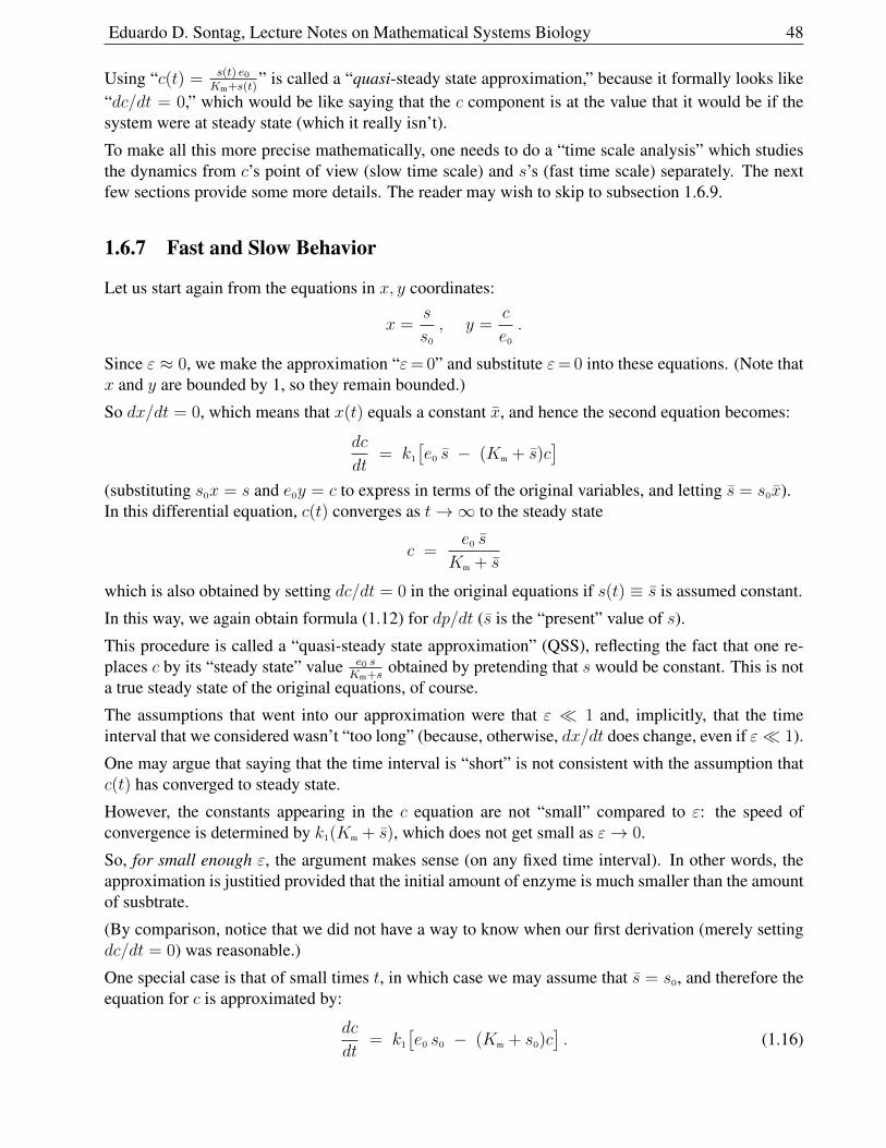
Eduardo D. Sontag, Lecture Notes on Mathematical Systems Biology 48
Using “c(t) = s(t) e0Km+s(t)
” is called a “quasi-steady state approximation,” because it formally looks like“dc/dt = 0,” which would be like saying that the c component is at the value that it would be if thesystem were at steady state (which it really isn’t).
To make all this more precise mathematically, one needs to do a “time scale analysis” which studiesthe dynamics from c’s point of view (slow time scale) and s’s (fast time scale) separately. The nextfew sections provide some more details. The reader may wish to skip to subsection 1.6.9.
1.6.7 Fast and Slow Behavior
Let us start again from the equations in x, y coordinates:
x =s
s0, y =
c
e0.
Since ε ≈ 0, we make the approximation “ε= 0” and substitute ε= 0 into these equations. (Note thatx and y are bounded by 1, so they remain bounded.)
So dx/dt = 0, which means that x(t) equals a constant x, and hence the second equation becomes:
dc
dt= k1
[e0 s − (Km + s)c
](substituting s0x = s and e0y = c to express in terms of the original variables, and letting s = s0x).In this differential equation, c(t) converges as t→∞ to the steady state
c =e0 s
Km + s
which is also obtained by setting dc/dt = 0 in the original equations if s(t) ≡ s is assumed constant.
In this way, we again obtain formula (1.12) for dp/dt (s is the “present” value of s).
This procedure is called a “quasi-steady state approximation” (QSS), reflecting the fact that one re-places c by its “steady state” value e0 s
Km+sobtained by pretending that s would be constant. This is not
a true steady state of the original equations, of course.
The assumptions that went into our approximation were that ε 1 and, implicitly, that the timeinterval that we considered wasn’t “too long” (because, otherwise, dx/dt does change, even if ε 1).
One may argue that saying that the time interval is “short” is not consistent with the assumption thatc(t) has converged to steady state.
However, the constants appearing in the c equation are not “small” compared to ε: the speed ofconvergence is determined by k1(Km + s), which does not get small as ε→ 0.
So, for small enough ε, the argument makes sense (on any fixed time interval). In other words, theapproximation is justitied provided that the initial amount of enzyme is much smaller than the amountof susbtrate.
(By comparison, notice that we did not have a way to know when our first derivation (merely settingdc/dt = 0) was reasonable.)
One special case is that of small times t, in which case we may assume that s = s0, and therefore theequation for c is approximated by:
dc
dt= k1
[e0 s0 − (Km + s0)c
]. (1.16)
Eduardo D. Sontag, Lecture Notes on Mathematical Systems Biology 49
One calls this the boundary layer equation, because it describes what happens near initial times(boundary of the time interval).
Long-time behavior (fast time scale)
Next, we ask what happens for those t “large enough” so that dx/dt ≈ 0 is not valid.
This is a question involving time-scale separation.
The intuitive idea is that c approaches its steady state value fast relative to the movement of s, whichis, therefore, supposed to be constant while this convergence happens.
Now we “iterate” the reasoning: s moves a bit, using c’s steady state value.
But then, c “reacts” to this new value of s, converging to a new steady state value (corresponding tothe new s), and the process is iterated in this fashion.
The problem with saying things in this manner is that, of course, it is not true that c and s take turnsmoving, but both move simultaneously (although at very different speeds).
In order to be more precise, it is convenient to make a change of time scale, using:
τ =e0s0k1t .
We may think of τ as a fast time scale, because τ = εk1t, and therefore τ is small for any given t.
For example, if εk1 = 1/3600 and t is measured in seconds, then τ = 10 implies that t = 36000; thus,“τ = 10” means that ten hours have elapsed, while “t = 10” means that only ten seconds elapsed.
Substituting s = s0x, c = e0y, and
dx
dτ=
1
e0k1
ds
dt,
dy
dτ=
s0e20k1
dc
dt,
we have:
dx
dτ=
k−1
k1
y − s0 x (1− y)
εdy
dτ= s0 x − (Km + s0 x)y .
Still assuming that ε 1, we make an approximation by setting ε = 0 in the second equation:
εdy
dτ= s0 x − (Km + s0 x)y
leading to the algebraic equation s0x − (Km + s0 x)y = 0 which we solve for y = y(x) = s0xKm+s0 x
,or equivalently
c =e0s
Km + s, (1.17)
and finally we substitute into the first equation:
dx
dτ=
k−1
k1
y − s0 x (1− y) = −(−k−1 +Kmk1) s0 x
k1(Km + s0 x)= − k2 s0 x
k1(Km + s0 x)
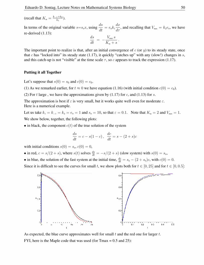
Eduardo D. Sontag, Lecture Notes on Mathematical Systems Biology 50
(recall that Km = k−1+k2k1
).
In terms of the original variable s=s0x, usingds
dt= e0k1
dx
dτ, and recalling that Vmax = k2e0, we have
re-derived (1.13):ds
dt= − Vmax s
Km + s.
The important point to realize is that, after an initial convergence of c (or y) to its steady state, oncethat c has “locked into” its steady state (1.17), it quickly “catches up” with any (slow!) changes in s,and this catch-up is not “visible” at the time scale τ , so c appears to track the expression (1.17).
Putting it all Together
Let’s suppose that s(0) = s0 and c(0) = c0.
(1) As we remarked earlier, for t ≈ 0 we have equation (1.16) (with initial condition c(0) = c0).
(2) For t large , we have the approximations given by (1.17) for c, and (1.13) for s.
The approximation is best if ε is very small, but it works quite well even for moderate ε.Here is a numerical example.
Let us take k1 = k−1 = k2 = e0 = 1 and s0 = 10, so that ε = 0.1. Note that Km = 2 and Vmax = 1.
We show below, together, the following plots:
• in black, the component c(t) of the true solution of the system
ds
dt= c− s(1− c) , dc
dt= s− (2 + s)c
with initial conditions s(0) = s0, c(0) = 0,
• in red, c = s/(2 + s), where s(t) solves dsdt
= −s/(2 + s) (slow system) with s(0) = s0,
• in blue, the solution of the fast system at the initial time, dcdt
= s0 − (2 + s0)c, with c(0) = 0.
Since it is difficult to see the curves for small t, we show plots both for t ∈ [0, 25] and for t ∈ [0, 0.5]:
As expected, the blue curve approximates well for small t and the red one for larger t.
FYI, here is the Maple code that was used (for Tmax = 0.5 and 25):
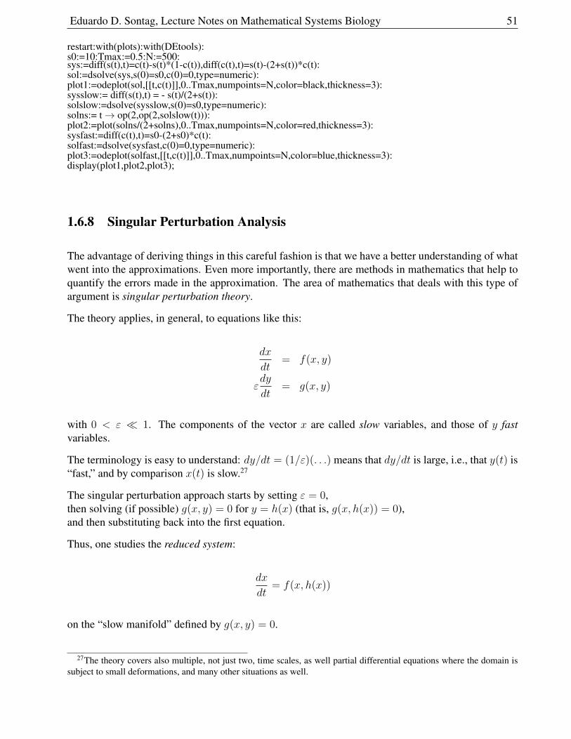
Eduardo D. Sontag, Lecture Notes on Mathematical Systems Biology 51
restart:with(plots):with(DEtools):s0:=10:Tmax:=0.5:N:=500:sys:=diff(s(t),t)=c(t)-s(t)*(1-c(t)),diff(c(t),t)=s(t)-(2+s(t))*c(t):sol:=dsolve(sys,s(0)=s0,c(0)=0,type=numeric):plot1:=odeplot(sol,[[t,c(t)]],0..Tmax,numpoints=N,color=black,thickness=3):sysslow:= diff(s(t),t) = - s(t)/(2+s(t)):solslow:=dsolve(sysslow,s(0)=s0,type=numeric):solns:= t→ op(2,op(2,solslow(t))):plot2:=plot(solns/(2+solns),0..Tmax,numpoints=N,color=red,thickness=3):sysfast:=diff(c(t),t)=s0-(2+s0)*c(t):solfast:=dsolve(sysfast,c(0)=0,type=numeric):plot3:=odeplot(solfast,[[t,c(t)]],0..Tmax,numpoints=N,color=blue,thickness=3):display(plot1,plot2,plot3);
1.6.8 Singular Perturbation Analysis
The advantage of deriving things in this careful fashion is that we have a better understanding of whatwent into the approximations. Even more importantly, there are methods in mathematics that help toquantify the errors made in the approximation. The area of mathematics that deals with this type ofargument is singular perturbation theory.
The theory applies, in general, to equations like this:
dx
dt= f(x, y)
εdy
dt= g(x, y)
with 0 < ε 1. The components of the vector x are called slow variables, and those of y fastvariables.
The terminology is easy to understand: dy/dt = (1/ε)(. . .) means that dy/dt is large, i.e., that y(t) is“fast,” and by comparison x(t) is slow.27
The singular perturbation approach starts by setting ε = 0,then solving (if possible) g(x, y) = 0 for y = h(x) (that is, g(x, h(x)) = 0),and then substituting back into the first equation.
Thus, one studies the reduced system:
dx
dt= f(x, h(x))
on the “slow manifold” defined by g(x, y) = 0.
27The theory covers also multiple, not just two, time scales, as well partial differential equations where the domain issubject to small deformations, and many other situations as well.
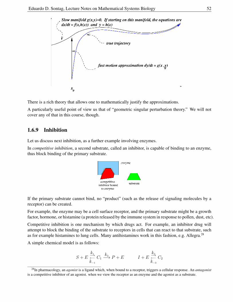
Eduardo D. Sontag, Lecture Notes on Mathematical Systems Biology 52
There is a rich theory that allows one to mathematically justify the approximations.
A particularly useful point of view us that of “geometric singular perturbation theory.” We will notcover any of that in this course, though.
1.6.9 Inhibition
Let us discuss next inhibition, as a further example involving enzymes.
In competitive inhibition, a second substrate, called an inhibitor, is capable of binding to an enzyme,thus block binding of the primary substrate.
If the primary substrate cannot bind, no “product” (such as the release of signaling molecules by areceptor) can be created.
For example, the enzyme may be a cell surface receptor, and the primary substrate might be a growthfactor, hormone, or histamine (a protein released by the immune system in response to pollen, dust, etc).
Competitive inhibition is one mechanism by which drugs act. For example, an inhibitor drug willattempt to block the binding of the substrate to receptors in cells that can react to that substrate, suchas for example histamines to lung cells. Many antihistamines work in this fashion, e.g. Allegra.28
A simple chemical model is as follows:
S + Ek1−→←−k−1
C1k2−→ P + E I + E
k3−→←−k−3
C2
28In pharmacology, an agonist is a ligand which, when bound to a receptor, triggers a cellular response. An antagonistis a competitive inhibitor of an agonist. when we view the receptor as an enzyme and the agonist as a substrate.
Eduardo D. Sontag, Lecture Notes on Mathematical Systems Biology 53
where C1 is the substrate/enzyme complex, C2 the inhibitor/enzyme complex, and I the inhibitor.
In terms of ODE’s, we have:ds
dt= k−1c1 − k1se
de
dt= (k−1 + k2)c1 + k−3c2 − k1se− k3ie
di
dt= k−3c2 − k3ie
dc1
dt= k1se− (k−1 + k2)c1
dc2
dt= k3ie− k−3c2
dp
dt= k2c1 .
It is easy to see that c1 + c2 + e is constant (it represents the total amount of free or bound enzyme,which we’ll denote as e0). This allows us to eliminate e from the equations. Furthermore, as before,we may first ignore the equation for p. We are left with a set of four ODE’s:
ds
dt= k−1c1 − k1s(e0 − c1 − c2)
di
dt= k−3c2 − k3ie
dc1
dt= k1s(e0 − c1 − c2)− (k−1 + k2)c1
dc2
dt= k3i(e0 − c1 − c2)− k−3c2 .
(We could also use a conservation law i + c2 ≡ i0 = total amount of inhibitor, free or bound toenzyme, to reduce to just three equations, but it is better for time-scale separation purposes not to doso.) One may now do a quasi-steady-state approximation, assuming that the enzyme concentrationsare small relative to substrate, amounting formally to setting dc1/dt = 0 and dc2/dt = 0. Doing sogives:
c1 =Kie0s
Kmi+Kis+KmKi
(Km =
k−1 + k2
k1
)c2 =
Kme0i
Kmi+Kis+KmKi
(Ki =
k−3
k3
).
The product formation rate is dp/dt = k2c1, so, again with Vmax = k2e0, one has the approximateformula:
dp
dt=
Vmax s
s+Km(1 + i/Ki)The formula reduces to the previous one if there is no inhibitor (i = 0).
We see that the rate of product formation is smaller than if there had been no inhibition, given thesame amount of substrate s(t) (at least if i1, k31, k−31).
But for s very large, the rate saturates at p = Vmax, just as if there was no inhibitor (intuitively, thereis so much s that i doesn’t get chance to bind and block). Thus, to affect the amount of product beingformed when the substrate amounts are large, potentially a huge amount of drug (inhibitor) wouldhave to be administered! Allosteric inhibition, described next, does not have the same disadvantage.
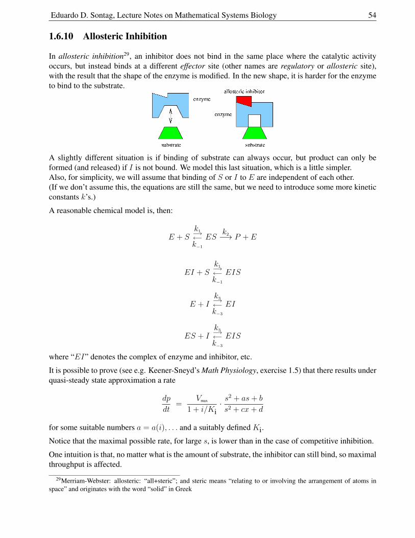
Eduardo D. Sontag, Lecture Notes on Mathematical Systems Biology 54
1.6.10 Allosteric Inhibition
In allosteric inhibition29, an inhibitor does not bind in the same place where the catalytic activityoccurs, but instead binds at a different effector site (other names are regulatory or allosteric site),with the result that the shape of the enzyme is modified. In the new shape, it is harder for the enzymeto bind to the substrate.
A slightly different situation is if binding of substrate can always occur, but product can only beformed (and released) if I is not bound. We model this last situation, which is a little simpler.Also, for simplicity, we will assume that binding of S or I to E are independent of each other.(If we don’t assume this, the equations are still the same, but we need to introduce some more kineticconstants k’s.)
A reasonable chemical model is, then:
E + Sk1−→←−k−1
ESk2−→ P + E
EI + Sk1−→←−k−1
EIS
E + Ik3−→←−k−3
EI
ES + Ik3−→←−k−3
EIS
where “EI” denotes the complex of enzyme and inhibitor, etc.
It is possible to prove (see e.g. Keener-Sneyd’s Math Physiology, exercise 1.5) that there results underquasi-steady state approximation a rate
dp
dt=
Vmax
1 + i/Ki· s
2 + as+ b
s2 + cx+ d
for some suitable numbers a = a(i), . . . and a suitably defined Ki.
Notice that the maximal possible rate, for large s, is lower than in the case of competitive inhibition.
One intuition is that, no matter what is the amount of substrate, the inhibitor can still bind, so maximalthroughput is affected.
29Merriam-Webster: allosteric: “all+steric”; and steric means “relating to or involving the arrangement of atoms inspace” and originates with the word “solid” in Greek
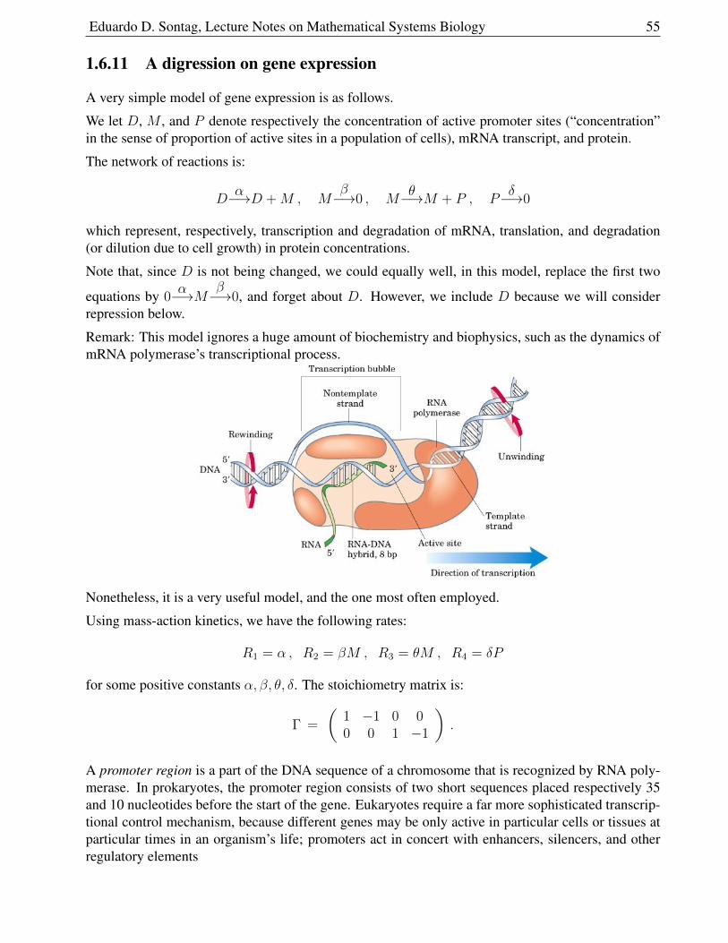
Eduardo D. Sontag, Lecture Notes on Mathematical Systems Biology 55
1.6.11 A digression on gene expression
A very simple model of gene expression is as follows.
We let D, M , and P denote respectively the concentration of active promoter sites (“concentration”in the sense of proportion of active sites in a population of cells), mRNA transcript, and protein.
The network of reactions is:
Dα−→D +M , M
β−→0 , Mθ−→M + P , P
δ−→0
which represent, respectively, transcription and degradation of mRNA, translation, and degradation(or dilution due to cell growth) in protein concentrations.
Note that, since D is not being changed, we could equally well, in this model, replace the first two
equations by 0α−→M β−→0, and forget about D. However, we include D because we will consider
repression below.
Remark: This model ignores a huge amount of biochemistry and biophysics, such as the dynamics ofmRNA polymerase’s transcriptional process.
Nonetheless, it is a very useful model, and the one most often employed.
Using mass-action kinetics, we have the following rates:
R1 = α , R2 = βM , R3 = θM , R4 = δP
for some positive constants α, β, θ, δ. The stoichiometry matrix is:
Γ =
(1 −1 0 00 0 1 −1
).
A promoter region is a part of the DNA sequence of a chromosome that is recognized by RNA poly-merase. In prokaryotes, the promoter region consists of two short sequences placed respectively 35and 10 nucleotides before the start of the gene. Eukaryotes require a far more sophisticated transcrip-tional control mechanism, because different genes may be only active in particular cells or tissues atparticular times in an organism’s life; promoters act in concert with enhancers, silencers, and otherregulatory elements
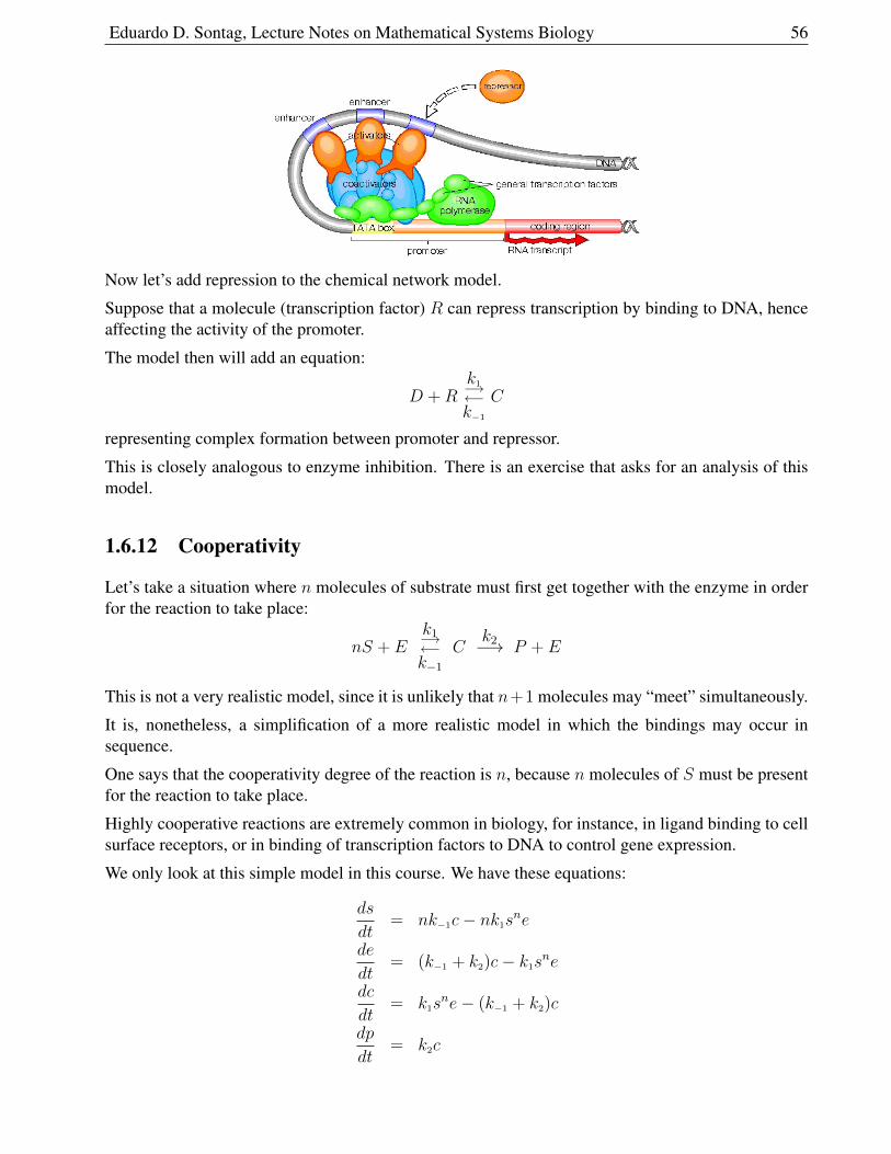
Eduardo D. Sontag, Lecture Notes on Mathematical Systems Biology 56
Now let’s add repression to the chemical network model.
Suppose that a molecule (transcription factor) R can repress transcription by binding to DNA, henceaffecting the activity of the promoter.
The model then will add an equation:
D +Rk1−→←−k−1
C
representing complex formation between promoter and repressor.
This is closely analogous to enzyme inhibition. There is an exercise that asks for an analysis of thismodel.
1.6.12 Cooperativity
Let’s take a situation where n molecules of substrate must first get together with the enzyme in orderfor the reaction to take place:
nS + Ek1−→←−k−1
Ck2−→ P + E
This is not a very realistic model, since it is unlikely that n+1 molecules may “meet” simultaneously.
It is, nonetheless, a simplification of a more realistic model in which the bindings may occur insequence.
One says that the cooperativity degree of the reaction is n, because n molecules of S must be presentfor the reaction to take place.
Highly cooperative reactions are extremely common in biology, for instance, in ligand binding to cellsurface receptors, or in binding of transcription factors to DNA to control gene expression.
We only look at this simple model in this course. We have these equations:
ds
dt= nk−1c− nk1s
ne
de
dt= (k−1 + k2)c− k1s
ne
dc
dt= k1s
ne− (k−1 + k2)c
dp
dt= k2c
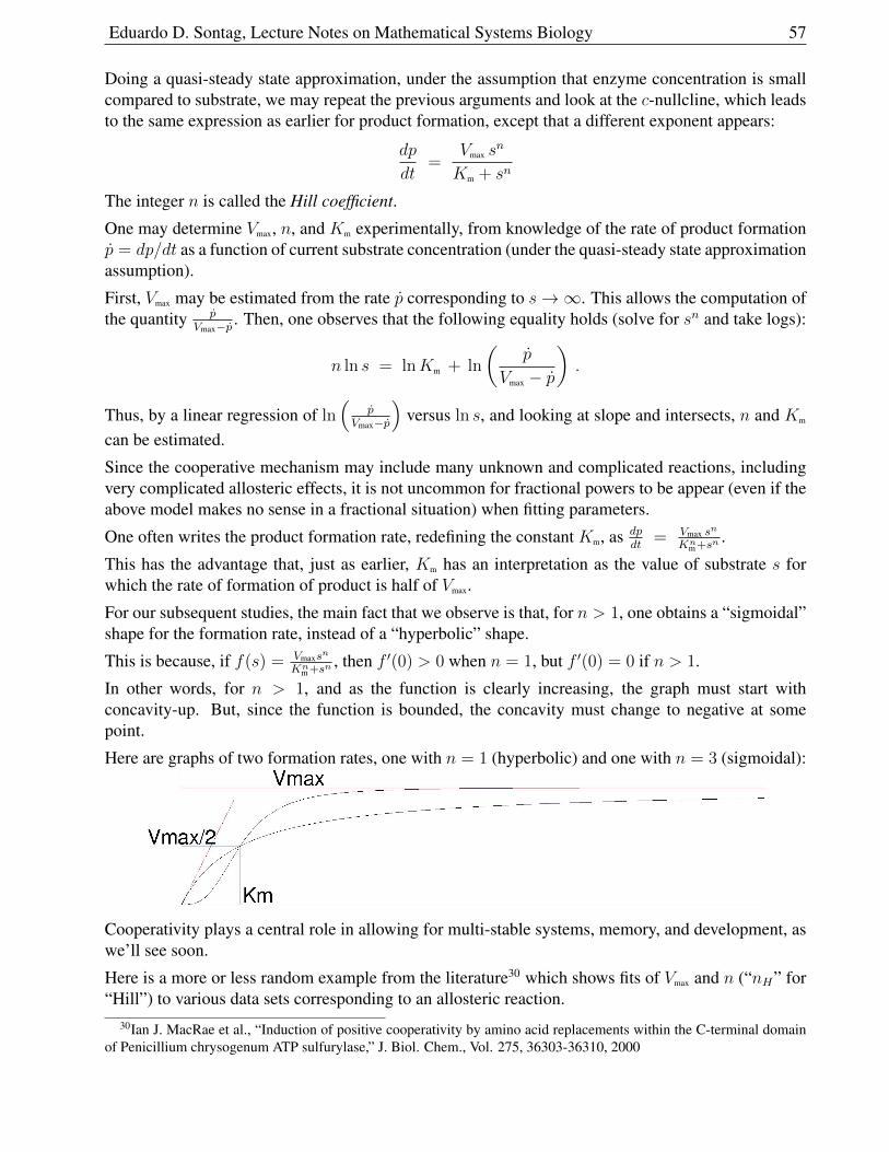
Eduardo D. Sontag, Lecture Notes on Mathematical Systems Biology 57
Doing a quasi-steady state approximation, under the assumption that enzyme concentration is smallcompared to substrate, we may repeat the previous arguments and look at the c-nullcline, which leadsto the same expression as earlier for product formation, except that a different exponent appears:
dp
dt=
Vmax sn
Km + sn
The integer n is called the Hill coefficient.
One may determine Vmax, n, and Km experimentally, from knowledge of the rate of product formationp = dp/dt as a function of current substrate concentration (under the quasi-steady state approximationassumption).
First, Vmax may be estimated from the rate p corresponding to s→∞. This allows the computation ofthe quantity p
Vmax−p . Then, one observes that the following equality holds (solve for sn and take logs):
n ln s = lnKm + ln
(p
Vmax − p
).
Thus, by a linear regression of ln(
pVmax−p
)versus ln s, and looking at slope and intersects, n and Km
can be estimated.
Since the cooperative mechanism may include many unknown and complicated reactions, includingvery complicated allosteric effects, it is not uncommon for fractional powers to be appear (even if theabove model makes no sense in a fractional situation) when fitting parameters.
One often writes the product formation rate, redefining the constant Km, as dpdt
= Vmax sn
Knm +sn
.
This has the advantage that, just as earlier, Km has an interpretation as the value of substrate s forwhich the rate of formation of product is half of Vmax.
For our subsequent studies, the main fact that we observe is that, for n > 1, one obtains a “sigmoidal”shape for the formation rate, instead of a “hyperbolic” shape.
This is because, if f(s) = Vmaxsn
Knm +sn
, then f ′(0) > 0 when n = 1, but f ′(0) = 0 if n > 1.
In other words, for n > 1, and as the function is clearly increasing, the graph must start withconcavity-up. But, since the function is bounded, the concavity must change to negative at somepoint.
Here are graphs of two formation rates, one with n = 1 (hyperbolic) and one with n = 3 (sigmoidal):
Cooperativity plays a central role in allowing for multi-stable systems, memory, and development, aswe’ll see soon.
Here is a more or less random example from the literature30 which shows fits of Vmax and n (“nH” for“Hill”) to various data sets corresponding to an allosteric reaction.
30Ian J. MacRae et al., “Induction of positive cooperativity by amino acid replacements within the C-terminal domainof Penicillium chrysogenum ATP sulfurylase,” J. Biol. Chem., Vol. 275, 36303-36310, 2000
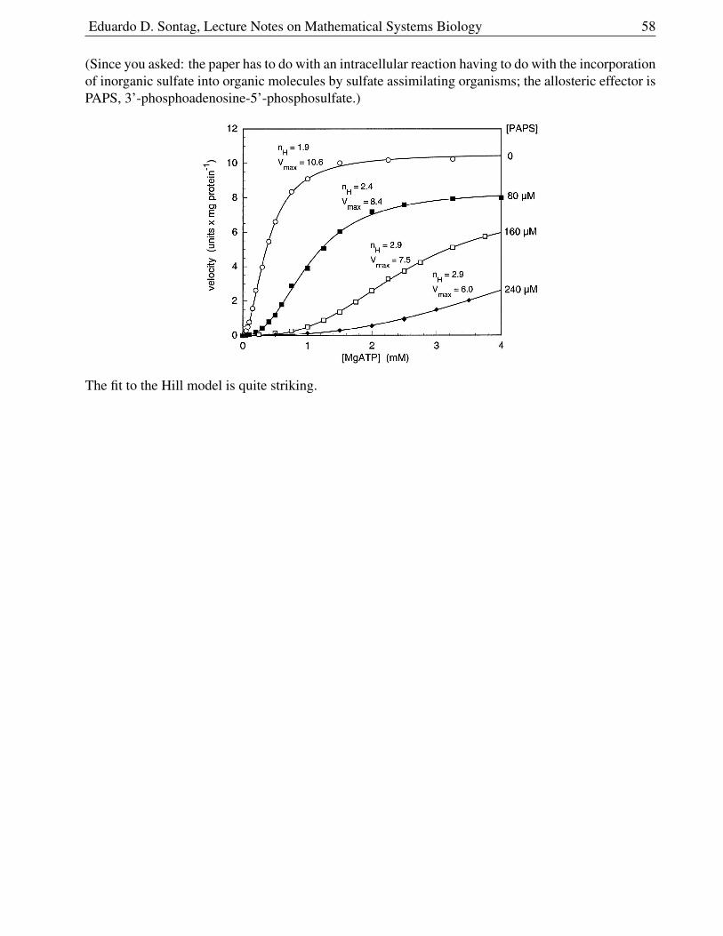
Eduardo D. Sontag, Lecture Notes on Mathematical Systems Biology 58
(Since you asked: the paper has to do with an intracellular reaction having to do with the incorporationof inorganic sulfate into organic molecules by sulfate assimilating organisms; the allosteric effector isPAPS, 3’-phosphoadenosine-5’-phosphosulfate.)
The fit to the Hill model is quite striking.
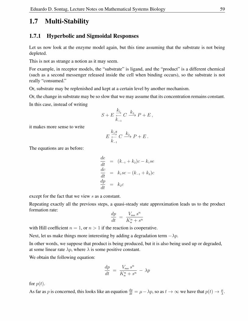
Eduardo D. Sontag, Lecture Notes on Mathematical Systems Biology 59
1.7 Multi-Stability
1.7.1 Hyperbolic and Sigmoidal Responses
Let us now look at the enzyme model again, but this time assuming that the substrate is not beingdepleted.
This is not as strange a notion as it may seem.
For example, in receptor models, the “substrate” is ligand, and the “product” is a different chemical(such as a second messenger released inside the cell when binding occurs), so the substrate is notreally “consumed.”
Or, substrate may be replenished and kept at a certain level by another mechanism.
Or, the change in substrate may be so slow that we may assume that its concentration remains constant.
In this case, instead of writing
S + Ek1−→←−k−1
Ck2−→ P + E ,
it makes more sense to write
Ek1s−→←−k−1
Ck2−→ P + E .
The equations are as before:
de
dt= (k−1 + k2)c− k1se
dc
dt= k1se− (k−1 + k2)c
dp
dt= k2c
except for the fact that we view s as a constant.
Repeating exactly all the previous steps, a quasi-steady state approximation leads us to the productformation rate:
dp
dt=
Vmax sn
Knm + sn
with Hill coefficient n = 1, or n > 1 if the reaction is cooperative.
Next, let us make things more interesting by adding a degradation term −λp.
In other words, we suppose that product is being produced, but it is also being used up or degraded,at some linear rate λp, where λ is some positive constant.
We obtain the following equation:
dp
dt=
Vmax sn
Knm + sn
− λp
for p(t).
As far as p is concerned, this looks like an equation dpdt
= µ−λp, so as t→∞ we have that p(t)→ µλ
.
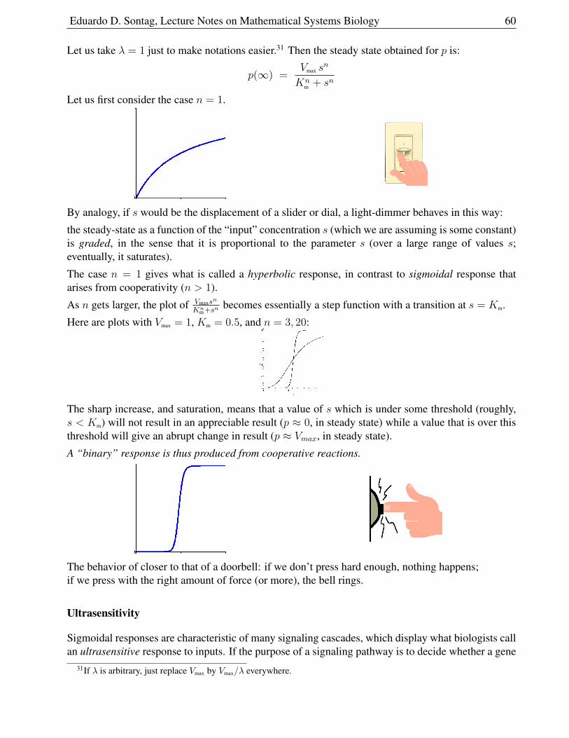
Eduardo D. Sontag, Lecture Notes on Mathematical Systems Biology 60
Let us take λ = 1 just to make notations easier.31 Then the steady state obtained for p is:
p(∞) =Vmax s
n
Knm + sn
Let us first consider the case n = 1.
By analogy, if s would be the displacement of a slider or dial, a light-dimmer behaves in this way:
the steady-state as a function of the “input” concentration s (which we are assuming is some constant)is graded, in the sense that it is proportional to the parameter s (over a large range of values s;eventually, it saturates).
The case n = 1 gives what is called a hyperbolic response, in contrast to sigmoidal response thatarises from cooperativity (n > 1).
As n gets larger, the plot of Vmaxsn
Knm +sn
becomes essentially a step function with a transition at s = Km.
Here are plots with Vmax = 1, Km = 0.5, and n = 3, 20:
The sharp increase, and saturation, means that a value of s which is under some threshold (roughly,s < Km) will not result in an appreciable result (p ≈ 0, in steady state) while a value that is over thisthreshold will give an abrupt change in result (p ≈ Vmax, in steady state).
A “binary” response is thus produced from cooperative reactions.
The behavior of closer to that of a doorbell: if we don’t press hard enough, nothing happens;if we press with the right amount of force (or more), the bell rings.
Ultrasensitivity
Sigmoidal responses are characteristic of many signaling cascades, which display what biologists callan ultrasensitive response to inputs. If the purpose of a signaling pathway is to decide whether a gene
31If λ is arbitrary, just replace Vmax by Vmax/λ everywhere.
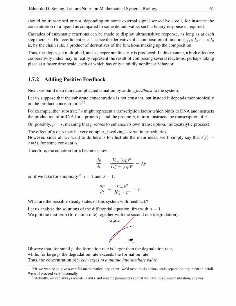
Eduardo D. Sontag, Lecture Notes on Mathematical Systems Biology 61
should be transcribed or not, depending on some external signal sensed by a cell, for instance theconcentration of a ligand as compared to some default value, such a binary response is required.
Cascades of enzymatic reactions can be made to display ultrasensitive response, as long as at eachstep there is a Hill coefficient n > 1, since the derivative of a composition of functions f1 f2 . . .fkis, by the chain rule, a product of derivatives of the functions making up the composition.
Thus, the slopes get multiplied, and a steeper nonlinearity is produced. In this manner, a high effectivecooperativity index may in reality represent the result of composing several reactions, perhaps takingplace at a faster time scale, each of which has only a mildly nonlinear behavior.
1.7.2 Adding Positive Feedback
Next, we build up a more complicated situation by adding feedback to the system.
Let us suppose that the substrate concentration is not constant, but instead it depends monotonicallyon the product concentration.32
For example, the “substrate” smight represent a transcription factor which binds to DNA and instructsthe production of mRNA for a protein p, and the protein p, in turn, instructs the transcription of s.
Or, possibly, p = s, meaning that p serves to enhance its own transcription. (autocatalytic process).
The effect of p on s may be very complex, involving several intermediaries.However, since all we want to do here is to illustrate the main ideas, we’ll simply say that s(t) =αp(t), for some constant α.
Therefore, the equation for p becomes now:
dp
dt=
Vmax (αp)n
Knm + (αp)n
− λp
or, if we take for simplicity33 α = 1 and λ = 1:
dp
dt=
Vmax pn
Knm + pn
− p .
What are the possible steady states of this system with feedback?
Let us analyze the solutions of the differential equation, first with n = 1.We plot the first term (formation rate) together with the second one (degradation):
Observe that, for small p, the formation rate is larger than the degradation rate,while, for large p, the degradation rate exceeds the formation rate.Thus, the concentration p(t) converges to a unique intermediate value.
32If we wanted to give a careful mathematical argument, we’d need to do a time-scale separation argument in detail.We will proceed very informally.
33Actually, we can always rescale p and t and rename parameters so that we have this simpler situation, anyway.
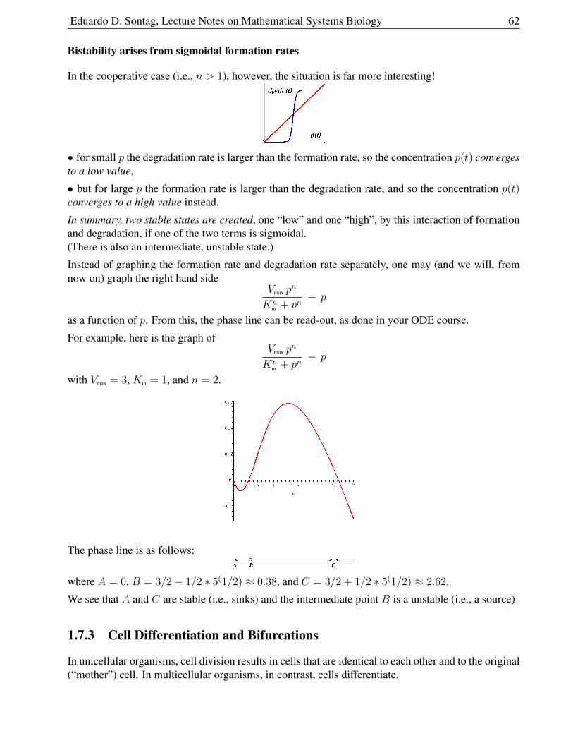
Eduardo D. Sontag, Lecture Notes on Mathematical Systems Biology 62
Bistability arises from sigmoidal formation rates
In the cooperative case (i.e., n > 1), however, the situation is far more interesting!
• for small p the degradation rate is larger than the formation rate, so the concentration p(t) convergesto a low value,
• but for large p the formation rate is larger than the degradation rate, and so the concentration p(t)converges to a high value instead.
In summary, two stable states are created, one “low” and one “high”, by this interaction of formationand degradation, if one of the two terms is sigmoidal.(There is also an intermediate, unstable state.)
Instead of graphing the formation rate and degradation rate separately, one may (and we will, fromnow on) graph the right hand side
Vmax pn
Knm + pn
− p
as a function of p. From this, the phase line can be read-out, as done in your ODE course.
For example, here is the graph ofVmax p
n
Knm + pn
− p
with Vmax = 3, Km = 1, and n = 2.
The phase line is as follows:
where A = 0, B = 3/2− 1/2 ∗ 5(1/2) ≈ 0.38, and C = 3/2 + 1/2 ∗ 5(1/2) ≈ 2.62.
We see that A and C are stable (i.e., sinks) and the intermediate point B is a unstable (i.e., a source)
1.7.3 Cell Differentiation and Bifurcations
In unicellular organisms, cell division results in cells that are identical to each other and to the original(“mother”) cell. In multicellular organisms, in contrast, cells differentiate.
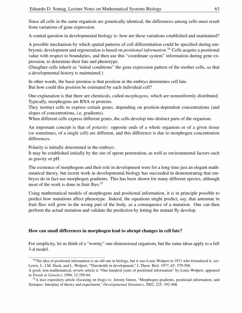
Eduardo D. Sontag, Lecture Notes on Mathematical Systems Biology 63
Since all cells in the same organism are genetically identical, the differences among cells must resultfrom variations of gene expression.
A central question in developmental biology is: how are these variations established and maintained?
A possible mechanism by which spatial patterns of cell differentiation could be specified during em-bryonic development and regeneration is based on positional information.34 Cells acquire a positionalvalue with respect to boundaries, and then use this “coordinate system” information during gene ex-pression, to determine their fate and phenotype.(Daughter cells inherit as “initial conditions” the gene expression pattern of the mother cells, so thata developmental history is maintained.)
In other words, the basic premise is that position in the embryo determines cell fate.But how could this position be estimated by each individual cell?
One explanation is that there are chemicals, called morphogens, which are nonuniformly distributed.Typically, morphogens are RNA or proteins.They instruct cells to express certain genes, depending on position-dependent concentrations (andslopes of concentrations, i.e. gradients).When different cells express different genes, the cells develop into distinct parts of the organism.
An important concept is that of polarity: opposite ends of a whole organism or of a given tissue(or sometimes, of a single cell) are different, and this difference is due to morphogen concentrationdifferences.
Polarity is initially determined in the embryo.It may be established initially by the site of sperm penetration, as well as environmental factors suchas gravity or pH.
The existence of morphogens and their role in development were for a long time just an elegant math-ematical theory, but recent work in developmental biology has succeeded in demonstrating that em-bryos do in fact use morphogen gradients. This has been shown for many different species, althoughmost of the work is done in fruit flies.35
Using mathematical models of morphogens and positional information, it is in principle possible topredict how mutations affect phenotype. Indeed, the equations might predict, say, that antennae infruit flies will grow in the wrong part of the body, as a consequence of a mutation. One can thenperform the actual mutation and validate the prediction by letting the mutant fly develop.
How can small differences in morphogen lead to abrupt changes in cell fate?
For simplicity, let us think of a “wormy” one-dimensional organism, but the same ideas apply to a full3-d model.
34The idea of positional information is an old one in biology, but it was Louis Wolpert in 1971 who formalized it, see:Lewis, J., J.M. Slack, and L. Wolpert, “Thresholds in development,” J. Theor. Biol. 1977, 65: 579-590.A good, non-mathematical, review article is “One hundred years of positional information” by Louis Wolpert, appearedin Trends in Genetics, 1996, 12:359-64.
35A nice expository article (focusing on frogs) is: Jeremy Green, “Morphogen gradients, positional information, andXenopus: Interplay of theory and experiment,” Developmental Dynamics, 2002, 225: 392-408.
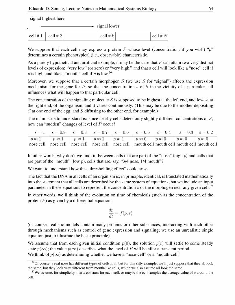
Eduardo D. Sontag, Lecture Notes on Mathematical Systems Biology 64
?-
cell # 1 cell # 2 cell # k cell # N
signal highest here
signal lower
We suppose that each cell may express a protein P whose level (concentration, if you wish) “p”determines a certain phenotypical (i.e., observable) characteristic.
As a purely hypothetical and artificial example, it may be the case that P can attain two very distinctlevels of expression: “very low” (or zero) or “very high,” and that a cell will look like a “nose” cell ifp is high, and like a “mouth” cell if p is low.36
Moreover, we suppose that a certain morphogen S (we use S for “signal”) affects the expressionmechanism for the gene for P , so that the concentration s of S in the vicinity of a particular cellinfluences what will happen to that particular cell.
The concentration of the signaling molecule S is supposed to be highest at the left end, and lowest atthe right end, of the organism, and it varies continuously. (This may be due to the mother depositingS at one end of the egg, and S diffusing to the other end, for example.)
The main issue to understand is: since nearby cells detect only slightly different concentrations of S,how can “sudden” changes of level of P occur?
s = 1 s = 0.9 s = 0.8 s = 0.7 s = 0.6 s = 0.5 s = 0.4 s = 0.3 s = 0.2
nose cell nose cell nose cell nose cell nose cell mouth cell mouth cell mouth cell mouth cellp ≈ 1 p ≈ 1 p ≈ 1 p ≈ 1p ≈ 1 p ≈ 0 p ≈ 0 p ≈ 0 p ≈ 0
In other words, why don’t we find, in-between cells that are part of the “nose” (high p) and cells thatare part of the “mouth” (low p), cells that are, say, “3/4 nose, 1/4 mouth”?
We want to understand how this “thresholding effect” could arise.
The fact that the DNA in all cells of an organism is, in principle, identical, is translated mathematicallyinto the statement that all cells are described by the same system of equations, but we include an inputparameter in these equations to represent the concentration s of the morphogen near any given cell.37
In other words, we’ll think of the evolution on time of chemicals (such as the concentration of theprotein P ) as given by a differential equation:
dp
dt= f(p, s)
(of course, realistic models contain many proteins or other substances, interacting with each otherthrough mechanisms such as control of gene expression and signaling; we use an unrealistic singleequation just to illustrate the basic principle).
We assume that from each given initial condition p(0), the solution p(t) will settle to some steadystate p(∞); the value p(∞) describes what the level of P will be after a transient period.We think of p(∞) as determining whether we have a “nose-cell” or a “mouth-cell.”
36Of course, a real nose has different types of cells in it, but for this silly example, we’ll just suppose that they all lookthe same, but they look very different from mouth-like cells, which we also assume all look the same.
37We assume, for simplicity, that s constant for each cell, or maybe the cell samples the average value of s around thecell.
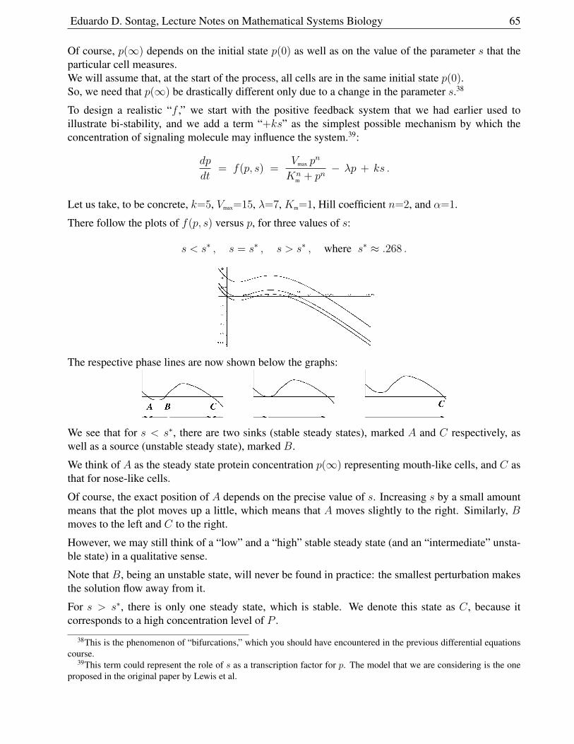
Eduardo D. Sontag, Lecture Notes on Mathematical Systems Biology 65
Of course, p(∞) depends on the initial state p(0) as well as on the value of the parameter s that theparticular cell measures.We will assume that, at the start of the process, all cells are in the same initial state p(0).So, we need that p(∞) be drastically different only due to a change in the parameter s.38
To design a realistic “f ,” we start with the positive feedback system that we had earlier used toillustrate bi-stability, and we add a term “+ks” as the simplest possible mechanism by which theconcentration of signaling molecule may influence the system.39:
dp
dt= f(p, s) =
Vmax pn
Knm + pn
− λp + ks .
Let us take, to be concrete, k=5, Vmax=15, λ=7, Km=1, Hill coefficient n=2, and α=1.
There follow the plots of f(p, s) versus p, for three values of s:
s < s∗ , s = s∗ , s > s∗ , where s∗ ≈ .268 .
The respective phase lines are now shown below the graphs:
We see that for s < s∗, there are two sinks (stable steady states), marked A and C respectively, aswell as a source (unstable steady state), marked B.
We think of A as the steady state protein concentration p(∞) representing mouth-like cells, and C asthat for nose-like cells.
Of course, the exact position of A depends on the precise value of s. Increasing s by a small amountmeans that the plot moves up a little, which means that A moves slightly to the right. Similarly, Bmoves to the left and C to the right.
However, we may still think of a “low” and a “high” stable steady state (and an “intermediate” unsta-ble state) in a qualitative sense.
Note that B, being an unstable state, will never be found in practice: the smallest perturbation makesthe solution flow away from it.
For s > s∗, there is only one steady state, which is stable. We denote this state as C, because itcorresponds to a high concentration level of P .
38This is the phenomenon of “bifurcations,” which you should have encountered in the previous differential equationscourse.
39This term could represent the role of s as a transcription factor for p. The model that we are considering is the oneproposed in the original paper by Lewis et al.
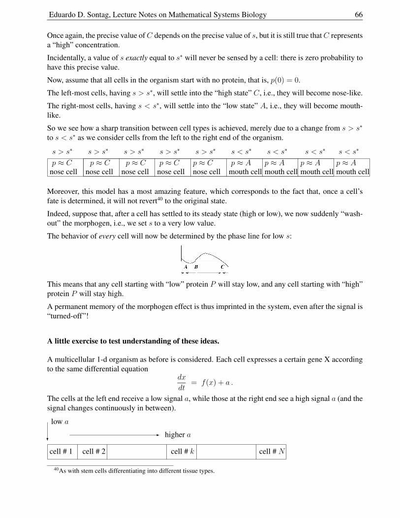
Eduardo D. Sontag, Lecture Notes on Mathematical Systems Biology 66
Once again, the precise value ofC depends on the precise value of s, but it is still true thatC representsa “high” concentration.
Incidentally, a value of s exactly equal to s∗ will never be sensed by a cell: there is zero probability tohave this precise value.
Now, assume that all cells in the organism start with no protein, that is, p(0) = 0.
The left-most cells, having s > s∗, will settle into the “high state” C, i.e., they will become nose-like.
The right-most cells, having s < s∗, will settle into the “low state” A, i.e., they will become mouth-like.
So we see how a sharp transition between cell types is achieved, merely due to a change from s > s∗
to s < s∗ as we consider cells from the left to the right end of the organism.
s > s∗ s > s∗ s > s∗ s > s∗ s > s∗ s < s∗ s < s∗ s < s∗ s < s∗
nose cell nose cell nose cell nose cell nose cell mouth cell mouth cell mouth cell mouth cellp ≈ C p ≈ C p ≈ C p ≈ Cp ≈ C p ≈ A p ≈ A p ≈ A p ≈ A
Moreover, this model has a most amazing feature, which corresponds to the fact that, once a cell’sfate is determined, it will not revert40 to the original state.
Indeed, suppose that, after a cell has settled to its steady state (high or low), we now suddenly “wash-out” the morphogen, i.e., we set s to a very low value.
The behavior of every cell will now be determined by the phase line for low s:
This means that any cell starting with “low” protein P will stay low, and any cell starting with “high”protein P will stay high.
A permanent memory of the morphogen effect is thus imprinted in the system, even after the signal is“turned-off”!
A little exercise to test understanding of these ideas.
A multicellular 1-d organism as before is considered. Each cell expresses a certain gene X accordingto the same differential equation
dx
dt= f(x) + a .
The cells at the left end receive a low signal a, while those at the right end see a high signal a (and thesignal changes continuously in between).
?-
cell # 1 cell # 2 cell # k cell # N
low a
higher a
40As with stem cells differentiating into different tissue types.
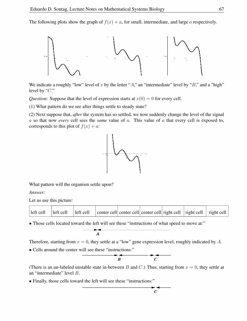
Eduardo D. Sontag, Lecture Notes on Mathematical Systems Biology 67
The following plots show the graph of f(x) + a, for small, intermediate, and large a respectively.
We indicate a roughly “low” level of x by the letter “A,” an “intermediate” level by “B,” and a ”high”level by “C.”
Question: Suppose that the level of expression starts at x(0) = 0 for every cell.
(1) What pattern do we see after things settle to steady state?
(2) Next suppose that, after the system has so settled, we now suddenly change the level of the signala so that now every cell sees the same value of a. This value of a that every cell is exposed to,corresponds to this plot of f(x) + a:
What pattern will the organism settle upon?
Answer:
Let us use this picture:
left cell left cell left cell center cell center cell center cell right cell right cell right cell
• Those cells located toward the left will see these “instructions of what speed to move at:”
Therefore, starting from x = 0, they settle at a “low” gene expression level, roughly indicated by A.
• Cells around the center will see these “instructions:”
(There is an un-labeled unstable state in-between B and C.) Thus, starting from x = 0, they settle atan “intermediate” level B.
• Finally, those cells toward the left will see these “instructions:”
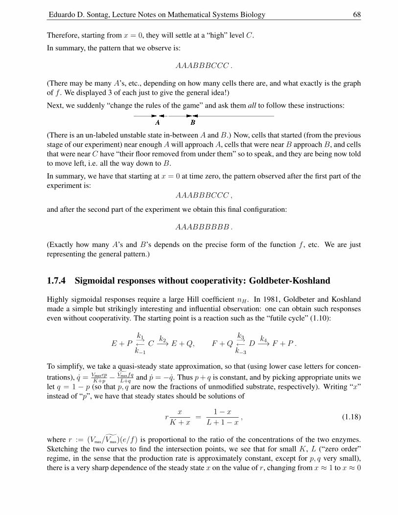
Eduardo D. Sontag, Lecture Notes on Mathematical Systems Biology 68
Therefore, starting from x = 0, they will settle at a “high” level C.
In summary, the pattern that we observe is:
AAABBBCCC .
(There may be many A’s, etc., depending on how many cells there are, and what exactly is the graphof f . We displayed 3 of each just to give the general idea!)
Next, we suddenly “change the rules of the game” and ask them all to follow these instructions:
(There is an un-labeled unstable state in-between A and B.) Now, cells that started (from the previousstage of our experiment) near enoughA will approachA, cells that were nearB approachB, and cellsthat were near C have “their floor removed from under them” so to speak, and they are being now toldto move left, i.e. all the way down to B.
In summary, we have that starting at x = 0 at time zero, the pattern observed after the first part of theexperiment is:
AAABBBCCC ,
and after the second part of the experiment we obtain this final configuration:
AAABBBBBB .
(Exactly how many A’s and B’s depends on the precise form of the function f , etc. We are justrepresenting the general pattern.)
1.7.4 Sigmoidal responses without cooperativity: Goldbeter-Koshland
Highly sigmoidal responses require a large Hill coefficient nH . In 1981, Goldbeter and Koshlandmade a simple but strikingly interesting and influential observation: one can obtain such responseseven without cooperativity. The starting point is a reaction such as the “futile cycle” (1.10):
E + Pk1−→←−k−1
Ck2−→ E +Q, F +Q
k3−→←−k−3
Dk4−→ F + P .
To simplify, we take a quasi-steady state approximation, so that (using lower case letters for concen-trations), q = Vmaxep
K+p− Vmaxfq
L+qand p = −q. Thus p+ q is constant, and by picking appropriate units we
let q = 1 − p (so that p, q are now the fractions of unmodified substrate, respectively). Writing “x”instead of “p”, we have that steady states should be solutions of
rx
K + x=
1− xL+ 1− x
, (1.18)
where r := (Vmax/Vmax)(e/f) is proportional to the ratio of the concentrations of the two enzymes.Sketching the two curves to find the intersection points, we see that for small K, L (“zero order”regime, in the sense that the production rate is approximately constant, except for p, q very small),there is a very sharp dependence of the steady state x on the value of r, changing from x ≈ 1 to x ≈ 0
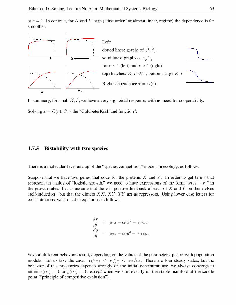
Eduardo D. Sontag, Lecture Notes on Mathematical Systems Biology 69
at r = 1. In contrast, for K and L large (“first order” or almost linear, regime) the dependence is farsmoother.
Left:
dotted lines: graphs of 1−xL+1−x
solid lines: graphs of r xK+x
for r < 1 (left) and r > 1 (right)
top sketches: K,L 1, bottom: large K,L
Right: dependence x = G(r)
In summary, for small K,L, we have a very sigmoidal response, with no need for cooperativity.
Solving x = G(r), G is the “GoldbeterKoshland function”.
1.7.5 Bistability with two species
There is a molecular-level analog of the “species competition” models in ecology, as follows.
Suppose that we have two genes that code for the proteins X and Y . In order to get terms thatrepresent an analog of “logistic growth,” we need to have expressions of the form “x(A − x)” inthe growth rates. Let us assume that there is positive feedback of each of X and Y on themselves(self-induction), but that the dimers XX , XY , Y Y act as repressors. Using lower case letters forconcentrations, we are led to equations as follows:
dx
dt= µ1x− α1x
2 − γ12xy
dy
dt= µ2y − α2y
2 − γ21xy .
Several different behaviors result, depending on the values of the parameters, just as with populationmodels. Let us take the case: α2/γ12 < µ1/µ2 < γ21/α1. There are four steady states, but thebehavior of the trajectories depends strongly on the initial concentrations: we always converge toeither x(∞) = 0 or y(∞) = 0, except when we start exactly on the stable manifold of the saddlepoint (“principle of competitive exclusion”).
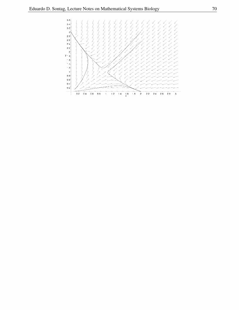
Eduardo D. Sontag, Lecture Notes on Mathematical Systems Biology 70
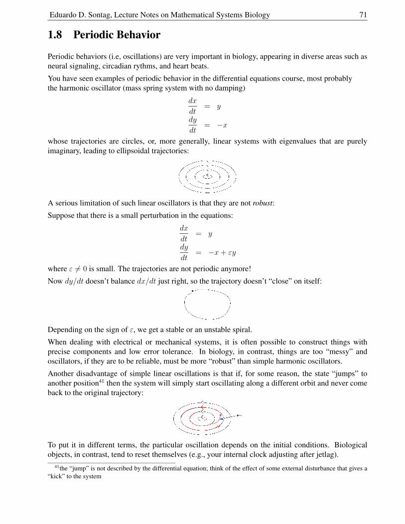
Eduardo D. Sontag, Lecture Notes on Mathematical Systems Biology 71
1.8 Periodic Behavior
Periodic behaviors (i.e, oscillations) are very important in biology, appearing in diverse areas such asneural signaling, circadian rythms, and heart beats.
You have seen examples of periodic behavior in the differential equations course, most probablythe harmonic oscillator (mass spring system with no damping)
dx
dt= y
dy
dt= −x
whose trajectories are circles, or, more generally, linear systems with eigenvalues that are purelyimaginary, leading to ellipsoidal trajectories:
A serious limitation of such linear oscillators is that they are not robust:
Suppose that there is a small perturbation in the equations:
dx
dt= y
dy
dt= −x+ εy
where ε 6= 0 is small. The trajectories are not periodic anymore!
Now dy/dt doesn’t balance dx/dt just right, so the trajectory doesn’t “close” on itself:
Depending on the sign of ε, we get a stable or an unstable spiral.
When dealing with electrical or mechanical systems, it is often possible to construct things withprecise components and low error tolerance. In biology, in contrast, things are too “messy” andoscillators, if they are to be reliable, must be more “robust” than simple harmonic oscillators.
Another disadvantage of simple linear oscillations is that if, for some reason, the state “jumps” toanother position41 then the system will simply start oscillating along a different orbit and never comeback to the original trajectory:
To put it in different terms, the particular oscillation depends on the initial conditions. Biologicalobjects, in contrast, tend to reset themselves (e.g., your internal clock adjusting after jetlag).
41the “jump” is not described by the differential equation; think of the effect of some external disturbance that gives a“kick” to the system
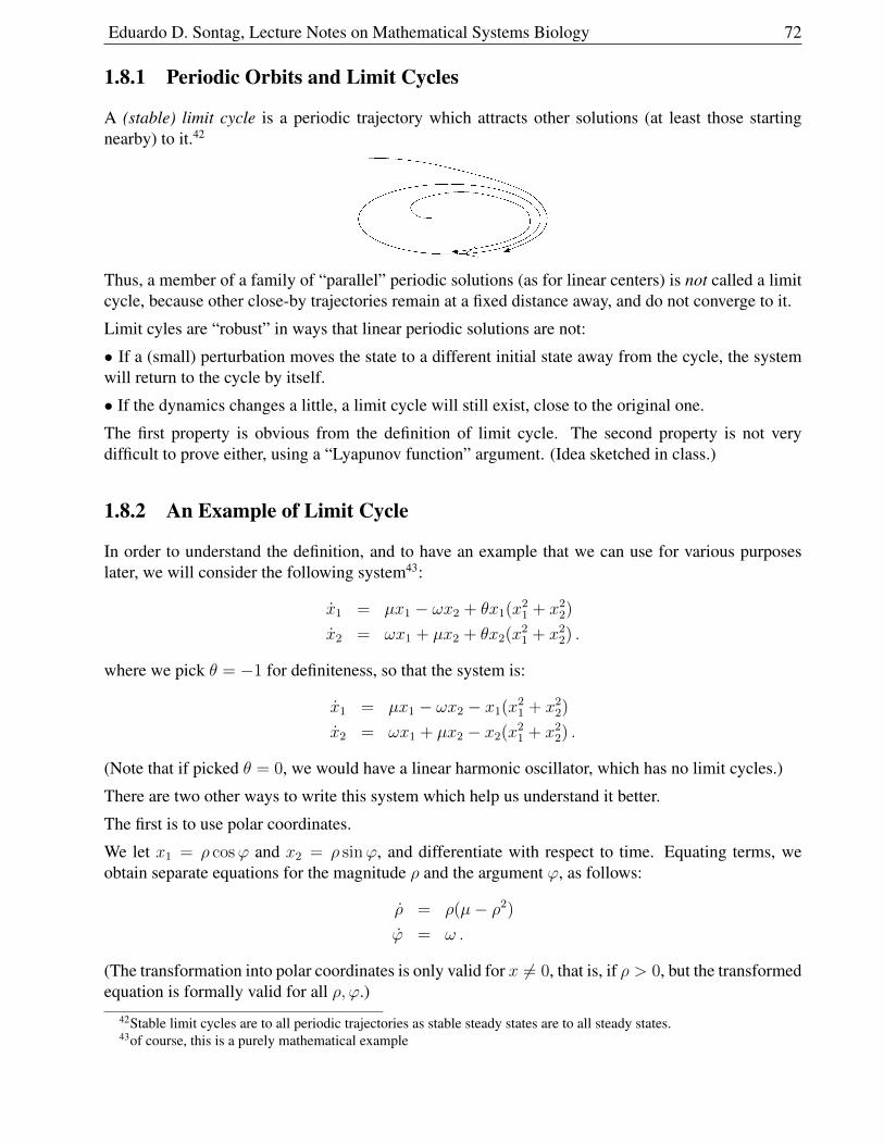
Eduardo D. Sontag, Lecture Notes on Mathematical Systems Biology 72
1.8.1 Periodic Orbits and Limit Cycles
A (stable) limit cycle is a periodic trajectory which attracts other solutions (at least those startingnearby) to it.42
Thus, a member of a family of “parallel” periodic solutions (as for linear centers) is not called a limitcycle, because other close-by trajectories remain at a fixed distance away, and do not converge to it.
Limit cyles are “robust” in ways that linear periodic solutions are not:
• If a (small) perturbation moves the state to a different initial state away from the cycle, the systemwill return to the cycle by itself.
• If the dynamics changes a little, a limit cycle will still exist, close to the original one.
The first property is obvious from the definition of limit cycle. The second property is not verydifficult to prove either, using a “Lyapunov function” argument. (Idea sketched in class.)
1.8.2 An Example of Limit Cycle
In order to understand the definition, and to have an example that we can use for various purposeslater, we will consider the following system43:
x1 = µx1 − ωx2 + θx1(x21 + x2
2)
x2 = ωx1 + µx2 + θx2(x21 + x2
2) .
where we pick θ = −1 for definiteness, so that the system is:
x1 = µx1 − ωx2 − x1(x21 + x2
2)
x2 = ωx1 + µx2 − x2(x21 + x2
2) .
(Note that if picked θ = 0, we would have a linear harmonic oscillator, which has no limit cycles.)
There are two other ways to write this system which help us understand it better.
The first is to use polar coordinates.
We let x1 = ρ cosϕ and x2 = ρ sinϕ, and differentiate with respect to time. Equating terms, weobtain separate equations for the magnitude ρ and the argument ϕ, as follows:
ρ = ρ(µ− ρ2)
ϕ = ω .
(The transformation into polar coordinates is only valid for x 6= 0, that is, if ρ > 0, but the transformedequation is formally valid for all ρ, ϕ.)
42Stable limit cycles are to all periodic trajectories as stable steady states are to all steady states.43of course, this is a purely mathematical example
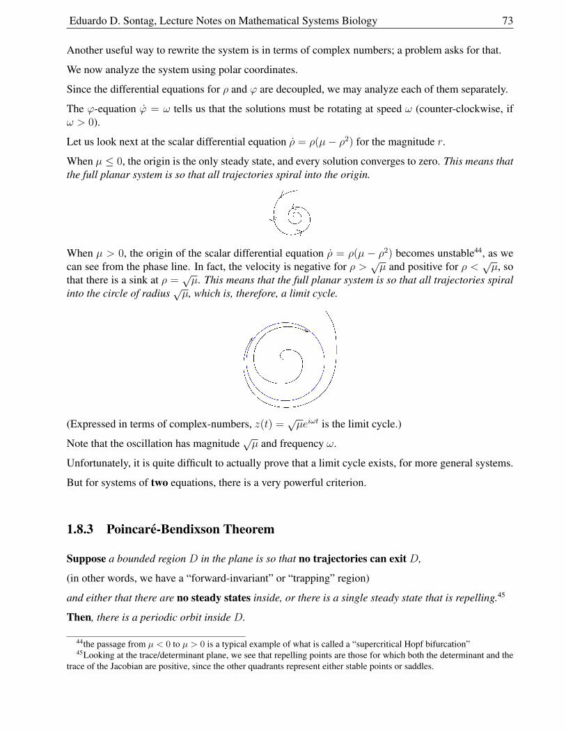
Eduardo D. Sontag, Lecture Notes on Mathematical Systems Biology 73
Another useful way to rewrite the system is in terms of complex numbers; a problem asks for that.
We now analyze the system using polar coordinates.
Since the differential equations for ρ and ϕ are decoupled, we may analyze each of them separately.
The ϕ-equation ϕ = ω tells us that the solutions must be rotating at speed ω (counter-clockwise, ifω > 0).
Let us look next at the scalar differential equation ρ = ρ(µ− ρ2) for the magnitude r.
When µ ≤ 0, the origin is the only steady state, and every solution converges to zero. This means thatthe full planar system is so that all trajectories spiral into the origin.
When µ > 0, the origin of the scalar differential equation ρ = ρ(µ − ρ2) becomes unstable44, as wecan see from the phase line. In fact, the velocity is negative for ρ >
√µ and positive for ρ <
õ, so
that there is a sink at ρ =√µ. This means that the full planar system is so that all trajectories spiral
into the circle of radiusõ, which is, therefore, a limit cycle.
(Expressed in terms of complex-numbers, z(t) =√µeiωt is the limit cycle.)
Note that the oscillation has magnitude√µ and frequency ω.
Unfortunately, it is quite difficult to actually prove that a limit cycle exists, for more general systems.
But for systems of two equations, there is a very powerful criterion.
1.8.3 Poincare-Bendixson Theorem
Suppose a bounded region D in the plane is so that no trajectories can exit D,
(in other words, we have a “forward-invariant” or “trapping” region)
and either that there are no steady states inside, or there is a single steady state that is repelling.45
Then, there is a periodic orbit inside D.
44the passage from µ < 0 to µ > 0 is a typical example of what is called a “supercritical Hopf bifurcation”45Looking at the trace/determinant plane, we see that repelling points are those for which both the determinant and the
trace of the Jacobian are positive, since the other quadrants represent either stable points or saddles.
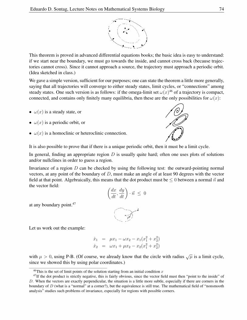
Eduardo D. Sontag, Lecture Notes on Mathematical Systems Biology 74
This theorem is proved in advanced differential equations books; the basic idea is easy to understand:if we start near the boundary, we must go towards the inside, and cannot cross back (because trajec-tories cannot cross). Since it cannot approach a source, the trajectory must approach a periodic orbit.(Idea sketched in class.)
We gave a simple version, sufficient for our purposes; one can state the theorem a little more generally,saying that all trajectories will converge to either steady states, limit cycles, or “connections” amongsteady states. One such version is as follows: if the omega-limit set ω(x)46 of a trajectory is compact,connected, and contains only finitely many equilibria, then these are the only possibilities for ω(x):
• ω(x) is a steady state, or
• ω(x) is a periodic orbit, or
• ω(x) is a homoclinic or heteroclinic connection.
It is also possible to prove that if there is a unique periodic orbit, then it must be a limit cycle.
In general, finding an appropriate region D is usually quite hard; often one uses plots of solutionsand/or nullclines in order to guess a region.
Invariance of a region D can be checked by using the following test: the outward-pointing normalvectors, at any point of the boundary of D, must make an angle of at least 90 degrees with the vectorfield at that point. Algebraically, this means that the dot product must be ≤ 0 between a normal ~n andthe vector field: (
dx
dt,dy
dt
)· ~n ≤ 0
at any boundary point.47
Let us work out the example:
x1 = µx1 − ωx2 − x1(x21 + x2
2)
x2 = ωx1 + µx2 − x2(x21 + x2
2)
with µ > 0, using P-B. (Of course, we already know that the circle with radius√µ is a limit cycle,
since we showed this by using polar coordinates.)
46This is the set of limit points of the solution starting from an initial condition x47If the dot product is strictly negative, this is fairly obvious, since the vector field must then “point to the inside” of
D. When the vectors are exactly perpendicular, the situation is a little more subtle, especially if there are corners in theboundary of D (what is a “normal” at a corner?), but the equivalence is still true. The mathematical field of “nonsmoothanalysis” studies such problems of invariance, especially for regions with possible corners.
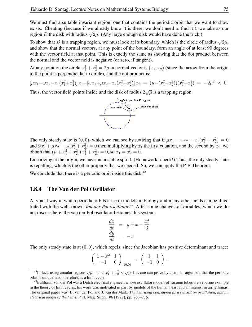
Eduardo D. Sontag, Lecture Notes on Mathematical Systems Biology 75
We must find a suitable invariant region, one that contains the periodic orbit that we want to showexists. Cheating (because if we already know it is there, we don’t need to find it!), we take as ourregion D the disk with radius
√2µ. (Any large enough disk would have done the trick.)
To show that D is a trapping region, we must look at its boundary, which is the circle of radius√
2µ,and show that the normal vectors, at any point of the boundary, form an angle of at least 90 degreeswith the vector field at that point. This is exactly the same as showing that the dot product betweenthe normal and the vector field is negative (or zero, if tangent).
At any point on the circle x21 + x2
2 = 2µ, a normal vector is (x1, x2) (since the arrow from the originto the point is perpendicular to circle), and the dot product is:
[µx1−ωx2−x1(x21+x2
2)]x1+[ωx1+µx2−x2(x21+x2
2)]x2 = (µ−(x21+x2
2))(x21+x2
2) = −2µ2 < 0 .
Thus, the vector field points inside and the disk of radius 2õ is a trapping region.
The only steady state is (0, 0), which we can see by noticing that if µx1 − ωx2 − x1(x21 + x2
2) = 0and ωx1 + µx2− x2(x2
1 + x22) = 0 then multiplying by x1 the first equation, and the second by x2, we
obtain that (µ+ x21 + x2
2)(x21 + x2
2) = 0, so x1 = x2 = 0.
Linearizing at the origin, we have an unstable spiral. (Homework: check!) Thus, the only steady stateis repelling, which is the other property that we needed. So, we can apply the P-B Theorem.
We conclude that there is a periodic orbit inside this disk.48
1.8.4 The Van der Pol Oscillator
A typical way in which periodic orbits arise in models in biology and many other fields can be illus-trated with the well-known Van der Pol oscillator.49 After some changes of variables, which we donot discuss here, the van der Pol oscillator becomes this system:
dx
dt= y + x− x3
3dy
dt= −x
The only steady state is at (0, 0), which repels, since the Jacobian has positive determinant and trace:(1− x2 1−1 0
)∣∣∣∣(0,0)
=
(1 1−1 0
).
48In fact, using annular regions√µ − ε < x21 + x22 <
√µ + ε, one can prove by a similar argument that the periodic
orbit is unique, and, therefore, is a limit cycle.49Balthazar van der Pol was a Dutch electrical engineer, whose oscillator models of vacuum tubes are a routine example
in the theory of limit cycles; his work was motivated in part by models of the human heart and an interest in arrhythmias.The original paper was: B. van der Pol and J. van der Mark, The heartbeat considered as a relaxation oscillation, and anelectrical model of the heart, Phil. Mag. Suppl. #6 (1928), pp. 763–775.
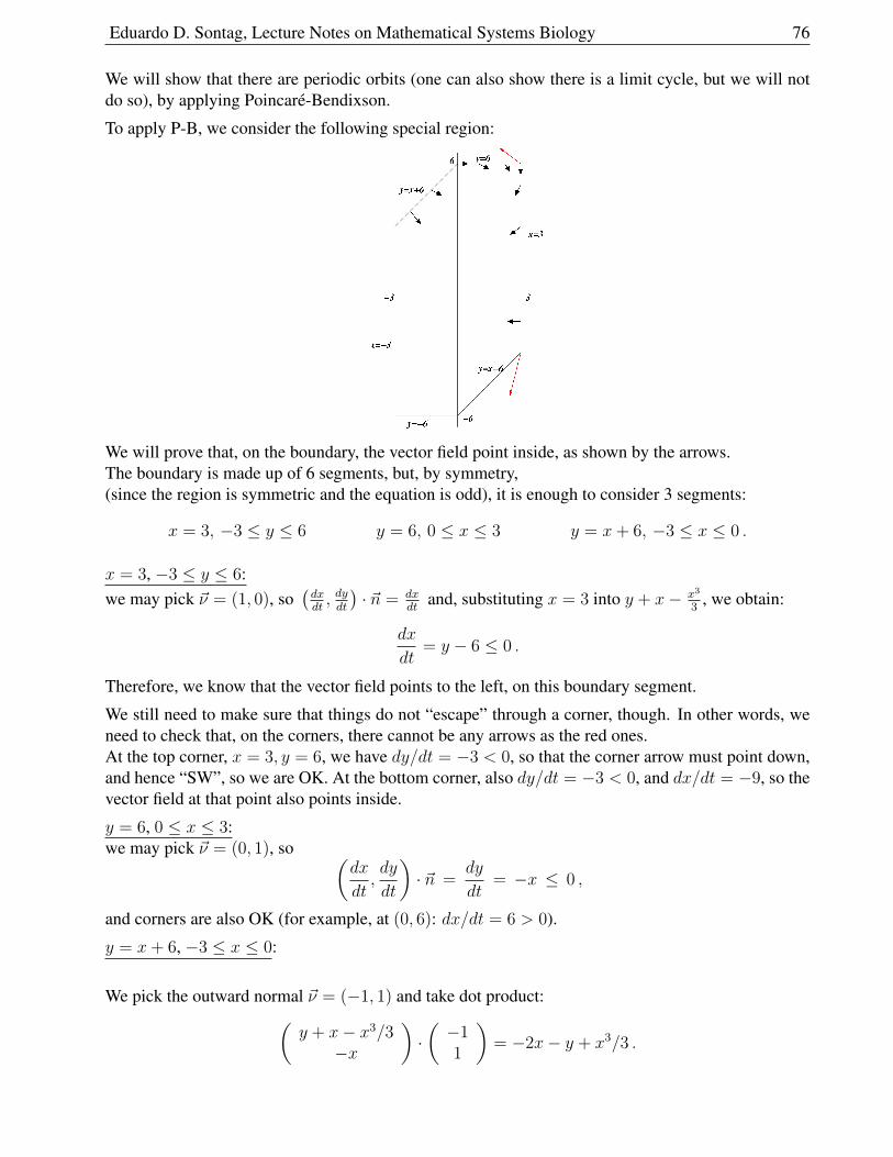
Eduardo D. Sontag, Lecture Notes on Mathematical Systems Biology 76
We will show that there are periodic orbits (one can also show there is a limit cycle, but we will notdo so), by applying Poincare-Bendixson.
To apply P-B, we consider the following special region:
We will prove that, on the boundary, the vector field point inside, as shown by the arrows.The boundary is made up of 6 segments, but, by symmetry,(since the region is symmetric and the equation is odd), it is enough to consider 3 segments:
x = 3, −3 ≤ y ≤ 6 y = 6, 0 ≤ x ≤ 3 y = x+ 6, −3 ≤ x ≤ 0 .
x = 3, −3 ≤ y ≤ 6:we may pick ~ν = (1, 0), so
(dxdt, dydt
)· ~n = dx
dtand, substituting x = 3 into y + x− x3
3, we obtain:
dx
dt= y − 6 ≤ 0 .
Therefore, we know that the vector field points to the left, on this boundary segment.
We still need to make sure that things do not “escape” through a corner, though. In other words, weneed to check that, on the corners, there cannot be any arrows as the red ones.At the top corner, x = 3, y = 6, we have dy/dt = −3 < 0, so that the corner arrow must point down,and hence “SW”, so we are OK. At the bottom corner, also dy/dt = −3 < 0, and dx/dt = −9, so thevector field at that point also points inside.
y = 6, 0 ≤ x ≤ 3:we may pick ~ν = (0, 1), so (
dx
dt,dy
dt
)· ~n =
dy
dt= −x ≤ 0 ,
and corners are also OK (for example, at (0, 6): dx/dt = 6 > 0).
y = x+ 6, −3 ≤ x ≤ 0:
We pick the outward normal ~ν = (−1, 1) and take dot product:(y + x− x3/3
−x
)·(−11
)= −2x− y + x3/3 .
Eduardo D. Sontag, Lecture Notes on Mathematical Systems Biology 77
Evaluated at y = x+ 6, this is:x3
3− 3x− 6, −3 ≤ x ≤ 0
which is indeed always negative (plot, or use calculus), and one can also check corners.
1.8.5 Bendixson’s Criterion
There is a useful criterion to help conclude there cannot be any periodic orbit in a given a simply-connected (no holes) region D:
If the divergence of the vector field is everywhere positive50 or is everywhere negative inside D,then there cannot be a periodic orbit inside D.
Sketch of proof (by contradiction):
Suppose that there is some such periodic orbit, which describes a simple closed curve C. We replacethe original D by the inside component of C; this set D is again simply-connected.
Recall that the divergence of F (x, y) =
(f(x, y)g(x, y)
)is defined as:
∂f
∂x+∂g
∂y.
The Gauss Divergence Theorem (or “Green’s Theorem”) says that:∫ ∫D
divF (x, y) dxdy =
∫C
~n · F
(the right-hand expression is the line integral of the dot product of a unit outward normal with F ).51
Now, saying that C is an orbit means that F is tangent to C, so the dot product is zero, and therefore∫ ∫D
divF (x, y) dxdy = 0 .
But, if divF (x, y) is everywhere positive, then the integral is positive, and we get a contradiction.Similarly if it is everywhere negative.
Example: dx/dt = x, dy/dt = y. Here the divergence is = 2 everywhere, so there cannot exist anyperiodic orbits (inside any region).
It is very important to realize what the theorem does not say:
Suppose that we take the example dx/dt = x, dy/dt = −y. Since the divergence is identically zero,the Bendixson criterion tells us nothing. In fact, this is a linear saddle, so we know (for other reasons)that there are no periodic obits.
On the other hand, for the example dx/dt = y, dy/dt = −x, which also has divergence identicallyzero, periodic orbits exist!
50To be precise, everywhere nonnegative but not everywhere zero51The one-dimensional analog of this is the Fundamental Theorem of Calculus: the integral of F ′ (which is the diver-
gence, when there is only one variable) over an interval [a, b] is equal to the integral over the boundary a, b of [a, b], thatis, F (b)− F (a).
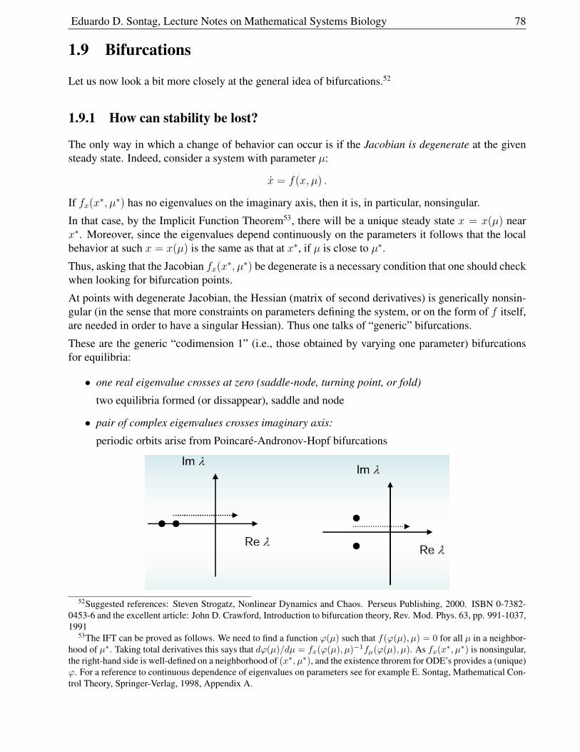
Eduardo D. Sontag, Lecture Notes on Mathematical Systems Biology 78
1.9 Bifurcations
Let us now look a bit more closely at the general idea of bifurcations.52
1.9.1 How can stability be lost?
The only way in which a change of behavior can occur is if the Jacobian is degenerate at the givensteady state. Indeed, consider a system with parameter µ:
x = f(x, µ) .
If fx(x∗, µ∗) has no eigenvalues on the imaginary axis, then it is, in particular, nonsingular.
In that case, by the Implicit Function Theorem53, there will be a unique steady state x = x(µ) nearx∗. Moreover, since the eigenvalues depend continuously on the parameters it follows that the localbehavior at such x = x(µ) is the same as that at x∗, if µ is close to µ∗.
Thus, asking that the Jacobian fx(x∗, µ∗) be degenerate is a necessary condition that one should checkwhen looking for bifurcation points.
At points with degenerate Jacobian, the Hessian (matrix of second derivatives) is generically nonsin-gular (in the sense that more constraints on parameters defining the system, or on the form of f itself,are needed in order to have a singular Hessian). Thus one talks of “generic” bifurcations.
These are the generic “codimension 1” (i.e., those obtained by varying one parameter) bifurcationsfor equilibria:
• one real eigenvalue crosses at zero (saddle-node, turning point, or fold)
two equilibria formed (or dissappear), saddle and node
• pair of complex eigenvalues crosses imaginary axis:
periodic orbits arise from Poincare-Andronov-Hopf bifurcations
52Suggested references: Steven Strogatz, Nonlinear Dynamics and Chaos. Perseus Publishing, 2000. ISBN 0-7382-0453-6 and the excellent article: John D. Crawford, Introduction to bifurcation theory, Rev. Mod. Phys. 63, pp. 991-1037,1991
53The IFT can be proved as follows. We need to find a function ϕ(µ) such that f(ϕ(µ), µ) = 0 for all µ in a neighbor-hood of µ∗. Taking total derivatives this says that dϕ(µ)/dµ = fx(ϕ(µ), µ)−1fµ(ϕ(µ), µ). As fx(x∗, µ∗) is nonsingular,the right-hand side is well-defined on a neighborhood of (x∗, µ∗), and the existence throrem for ODE’s provides a (unique)ϕ. For a reference to continuous dependence of eigenvalues on parameters see for example E. Sontag, Mathematical Con-trol Theory, Springer-Verlag, 1998, Appendix A.
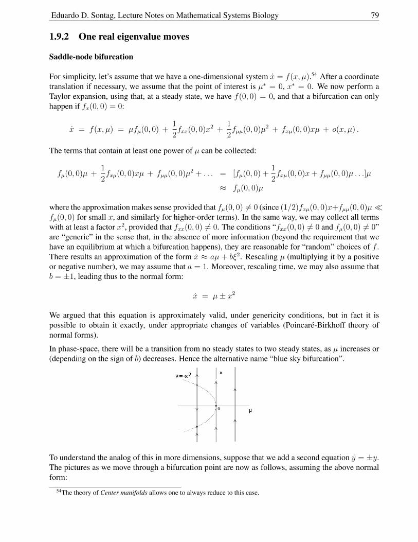
Eduardo D. Sontag, Lecture Notes on Mathematical Systems Biology 79
1.9.2 One real eigenvalue moves
Saddle-node bifurcation
For simplicity, let’s assume that we have a one-dimensional system x = f(x, µ).54 After a coordinatetranslation if necessary, we assume that the point of interest is µ∗ = 0, x∗ = 0. We now perform aTaylor expansion, using that, at a steady state, we have f(0, 0) = 0, and that a bifurcation can onlyhappen if fx(0, 0) = 0:
x = f(x, µ) = µfµ(0, 0) +1
2fxx(0, 0)x2 +
1
2fµµ(0, 0)µ2 + fxµ(0, 0)xµ + o(x, µ) .
The terms that contain at least one power of µ can be collected:
fµ(0, 0)µ +1
2fxµ(0, 0)xµ + fµµ(0, 0)µ2 + . . . = [fµ(0, 0) +
1
2fxµ(0, 0)x+ fµµ(0, 0)µ . . .]µ
≈ fµ(0, 0)µ
where the approximation makes sense provided that fµ(0, 0) 6= 0 (since (1/2)fxµ(0, 0)x+fµµ(0, 0)µfµ(0, 0) for small x, and similarly for higher-order terms). In the same way, we may collect all termswith at least a factor x2, provided that fxx(0, 0) 6= 0. The conditions “fxx(0, 0) 6= 0 and fµ(0, 0) 6= 0”are “generic” in the sense that, in the absence of more information (beyond the requirement that wehave an equilibrium at which a bifurcation happens), they are reasonable for “random” choices of f .There results an approximation of the form x ≈ aµ + bξ2. Rescaling µ (multiplying it by a positiveor negative number), we may assume that a = 1. Moreover, rescaling time, we may also assume thatb = ±1, leading thus to the normal form:
x = µ± x2
We argued that this equation is approximately valid, under genericity conditions, but in fact it ispossible to obtain it exactly, under appropriate changes of variables (Poincare-Birkhoff theory ofnormal forms).
In phase-space, there will be a transition from no steady states to two steady states, as µ increases or(depending on the sign of b) decreases. Hence the alternative name “blue sky bifurcation”.
To understand the analog of this in more dimensions, suppose that we add a second equation y = ±y.The pictures as we move through a bifurcation point are now as follows, assuming the above normalform:
54The theory of Center manifolds allows one to always reduce to this case.
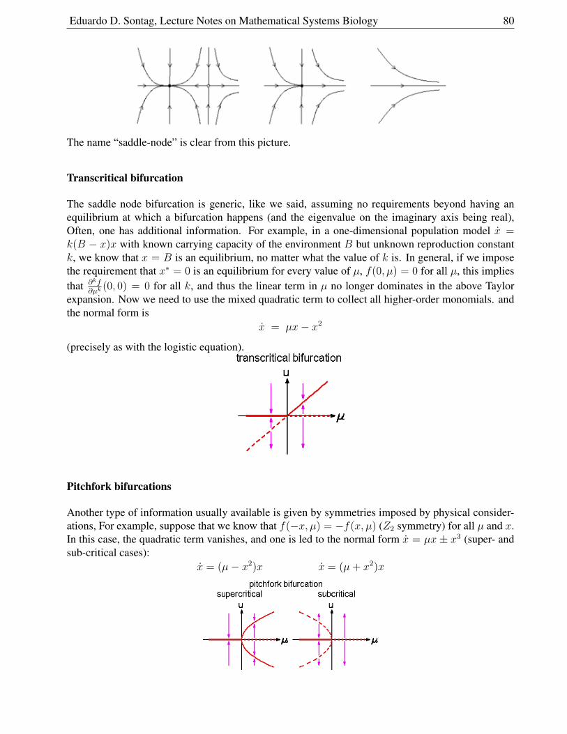
Eduardo D. Sontag, Lecture Notes on Mathematical Systems Biology 80
The name “saddle-node” is clear from this picture.
Transcritical bifurcation
The saddle node bifurcation is generic, like we said, assuming no requirements beyond having anequilibrium at which a bifurcation happens (and the eigenvalue on the imaginary axis being real),Often, one has additional information. For example, in a one-dimensional population model x =k(B − x)x with known carrying capacity of the environment B but unknown reproduction constantk, we know that x = B is an equilibrium, no matter what the value of k is. In general, if we imposethe requirement that x∗ = 0 is an equilibrium for every value of µ, f(0, µ) = 0 for all µ, this impliesthat ∂kf
∂µk(0, 0) = 0 for all k, and thus the linear term in µ no longer dominates in the above Taylor
expansion. Now we need to use the mixed quadratic term to collect all higher-order monomials. andthe normal form is
x = µx− x2
(precisely as with the logistic equation).
Pitchfork bifurcations
Another type of information usually available is given by symmetries imposed by physical consider-ations, For example, suppose that we know that f(−x, µ) = −f(x, µ) (Z2 symmetry) for all µ and x.In this case, the quadratic term vanishes, and one is led to the normal form x = µx ± x3 (super- andsub-critical cases):
x = (µ− x2)x x = (µ+ x2)x
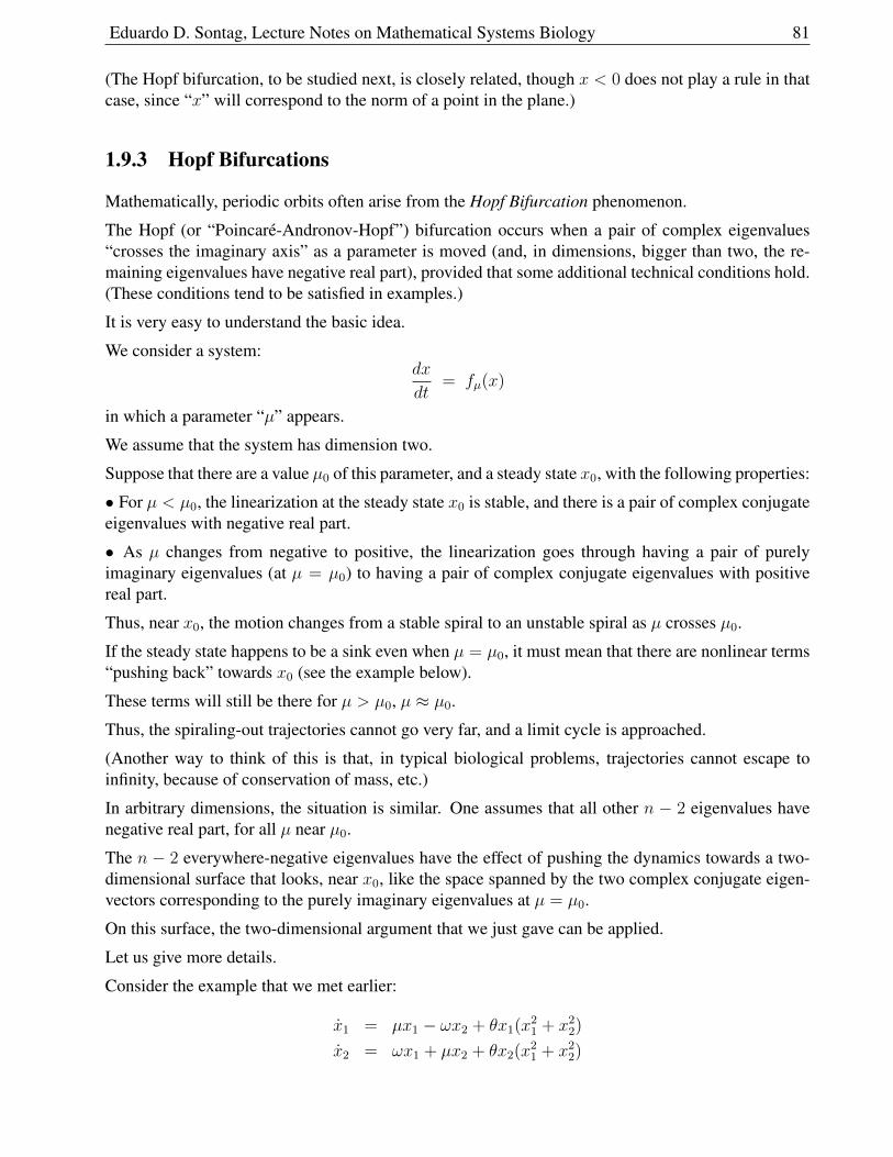
Eduardo D. Sontag, Lecture Notes on Mathematical Systems Biology 81
(The Hopf bifurcation, to be studied next, is closely related, though x < 0 does not play a rule in thatcase, since “x” will correspond to the norm of a point in the plane.)
1.9.3 Hopf Bifurcations
Mathematically, periodic orbits often arise from the Hopf Bifurcation phenomenon.
The Hopf (or “Poincare-Andronov-Hopf”) bifurcation occurs when a pair of complex eigenvalues“crosses the imaginary axis” as a parameter is moved (and, in dimensions, bigger than two, the re-maining eigenvalues have negative real part), provided that some additional technical conditions hold.(These conditions tend to be satisfied in examples.)
It is very easy to understand the basic idea.
We consider a system:dx
dt= fµ(x)
in which a parameter “µ” appears.
We assume that the system has dimension two.
Suppose that there are a value µ0 of this parameter, and a steady state x0, with the following properties:
• For µ < µ0, the linearization at the steady state x0 is stable, and there is a pair of complex conjugateeigenvalues with negative real part.
• As µ changes from negative to positive, the linearization goes through having a pair of purelyimaginary eigenvalues (at µ = µ0) to having a pair of complex conjugate eigenvalues with positivereal part.
Thus, near x0, the motion changes from a stable spiral to an unstable spiral as µ crosses µ0.
If the steady state happens to be a sink even when µ = µ0, it must mean that there are nonlinear terms“pushing back” towards x0 (see the example below).
These terms will still be there for µ > µ0, µ ≈ µ0.
Thus, the spiraling-out trajectories cannot go very far, and a limit cycle is approached.
(Another way to think of this is that, in typical biological problems, trajectories cannot escape toinfinity, because of conservation of mass, etc.)
In arbitrary dimensions, the situation is similar. One assumes that all other n − 2 eigenvalues havenegative real part, for all µ near µ0.
The n − 2 everywhere-negative eigenvalues have the effect of pushing the dynamics towards a two-dimensional surface that looks, near x0, like the space spanned by the two complex conjugate eigen-vectors corresponding to the purely imaginary eigenvalues at µ = µ0.
On this surface, the two-dimensional argument that we just gave can be applied.
Let us give more details.
Consider the example that we met earlier:
x1 = µx1 − ωx2 + θx1(x21 + x2
2)
x2 = ωx1 + µx2 + θx2(x21 + x2
2)
Eduardo D. Sontag, Lecture Notes on Mathematical Systems Biology 82
With θ = −1, this is the “supercritical Hopf bifurcation” case in which we go, as already shown, froma globally asymptotically stable equilibrium to a limit cycle as µ crosses from negative to positive (µ0
is zero).
In contrast, suppose now that θ = 1. The magnitude satisfies the equation ρ = ρ(µ+ ρ2).
Hence, one goes again from stable to unstable as µ goes through zero, but now an unstable cycleencircles the origin for µ < 0 (so, the origin is not globally attractive).
For µ ≥ 0, there is now no cycle that prevents solutions that start near zero from escaping very far.(Once again, in typical biochemical problems, solutions cannot go to infinity. So, for example, a limitcycle of large magnitude might perhaps appear for µ > 0.)
These pictures shows what happens for each fixed value of µ for the supercritical (limit cycle occursafter going from stable to unstable) and subcritical (limit cycle occurs before µ0) cases, respectively:
Now suppose given a general system (I will not ask questions in tests about this material; it is merelyFYI)55:
x = f(x, µ)
in dimension 2, where µ is a scalar parameter and f is assumed smooth. Suppose that for all µnear zero there is a steady-state ξ(µ), with eigenvalues λ(µ) = r(µ) ± iω(µ), with r(0) = 0 andω(0) = ω0 > 0, and that r′(0) 6= 0 (“eigenvalues cross the imaginary axis with nonzero velocity”)and that the quantity α defined below is nonzero. Then, up to a local topological equivalence andtime-reparametrization, one can reduce the system to the form given in the previous example, andthere is a Hopf bifurcation, supercritical or subcritical depending on θ = the sign of α.56 There isno need to perform the transformation, if all we want is to decide if there is a Hopf bifurcation. Thegeneral “recipe” is as follows.
Let A be the Jacobian of f evaluated at ξ0 = ξ(0), µ = 0. and find two complex vectors p, q such that
Aq = iω0q , ATp = −iω0p , p · q = 1 .
Compute the dot product H(z, z) = p · F (ξ0 + zq + zq, µ(0)) and consider the formal Taylor series:
H(z, z) = iω0z +∑j+k≥2
1
j!k!gjkz
j zk .
55See e.g. Yu.A. Kuznetsov. Elements of Applied Bifurcation Theory. 2nd ed., Springer-Verlag, New York, 199856One may interpret the condition on α in terms of a Lyapunov function that guarantees stability at µ = 0, for the
supercritical case; see e.g.: Mees , A.I. Dynamics of Feedback Systems, John Wiley & Sons, New York, 1981.
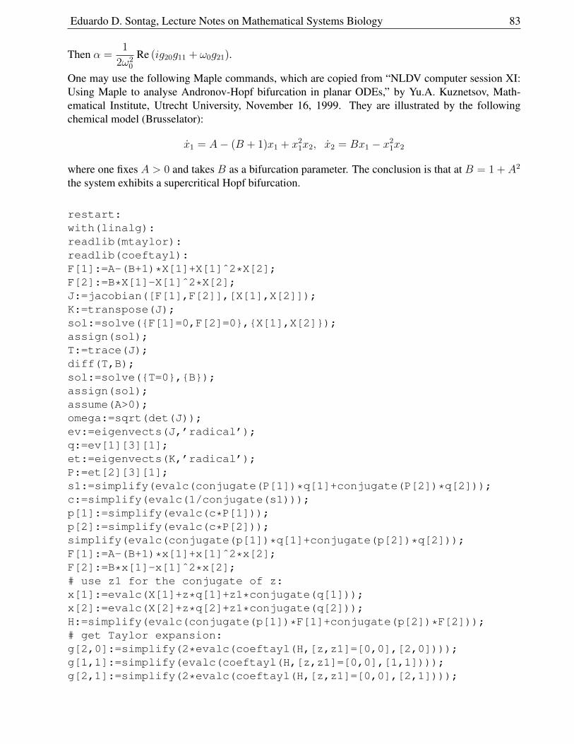
Eduardo D. Sontag, Lecture Notes on Mathematical Systems Biology 83
Then α =1
2ω20
Re (ig20g11 + ω0g21).
One may use the following Maple commands, which are copied from “NLDV computer session XI:Using Maple to analyse Andronov-Hopf bifurcation in planar ODEs,” by Yu.A. Kuznetsov, Math-ematical Institute, Utrecht University, November 16, 1999. They are illustrated by the followingchemical model (Brusselator):
x1 = A− (B + 1)x1 + x21x2, x2 = Bx1 − x2
1x2
where one fixes A > 0 and takes B as a bifurcation parameter. The conclusion is that at B = 1 + A2
the system exhibits a supercritical Hopf bifurcation.
restart:with(linalg):readlib(mtaylor):readlib(coeftayl):F[1]:=A-(B+1)*X[1]+X[1]ˆ2*X[2];F[2]:=B*X[1]-X[1]ˆ2*X[2];J:=jacobian([F[1],F[2]],[X[1],X[2]]);K:=transpose(J);sol:=solve(F[1]=0,F[2]=0,X[1],X[2]);assign(sol);T:=trace(J);diff(T,B);sol:=solve(T=0,B);assign(sol);assume(A>0);omega:=sqrt(det(J));ev:=eigenvects(J,’radical’);q:=ev[1][3][1];et:=eigenvects(K,’radical’);P:=et[2][3][1];s1:=simplify(evalc(conjugate(P[1])*q[1]+conjugate(P[2])*q[2]));c:=simplify(evalc(1/conjugate(s1)));p[1]:=simplify(evalc(c*P[1]));p[2]:=simplify(evalc(c*P[2]));simplify(evalc(conjugate(p[1])*q[1]+conjugate(p[2])*q[2]));F[1]:=A-(B+1)*x[1]+x[1]ˆ2*x[2];F[2]:=B*x[1]-x[1]ˆ2*x[2];# use z1 for the conjugate of z:x[1]:=evalc(X[1]+z*q[1]+z1*conjugate(q[1]));x[2]:=evalc(X[2]+z*q[2]+z1*conjugate(q[2]));H:=simplify(evalc(conjugate(p[1])*F[1]+conjugate(p[2])*F[2]));# get Taylor expansion:g[2,0]:=simplify(2*evalc(coeftayl(H,[z,z1]=[0,0],[2,0])));g[1,1]:=simplify(evalc(coeftayl(H,[z,z1]=[0,0],[1,1])));g[2,1]:=simplify(2*evalc(coeftayl(H,[z,z1]=[0,0],[2,1])));
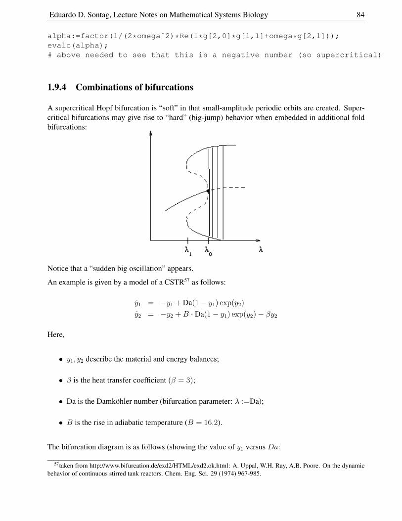
Eduardo D. Sontag, Lecture Notes on Mathematical Systems Biology 84
alpha:=factor(1/(2*omegaˆ2)*Re(I*g[2,0]*g[1,1]+omega*g[2,1]));evalc(alpha);# above needed to see that this is a negative number (so supercritical)
1.9.4 Combinations of bifurcations
A supercritical Hopf bifurcation is “soft” in that small-amplitude periodic orbits are created. Super-critical bifurcations may give rise to “hard” (big-jump) behavior when embedded in additional foldbifurcations:
Notice that a “sudden big oscillation” appears.
An example is given by a model of a CSTR57 as follows:
y1 = −y1 + Da(1− y1) exp(y2)
y2 = −y2 +B · Da(1− y1) exp(y2)− βy2
Here,
• y1, y2 describe the material and energy balances;
• β is the heat transfer coefficient (β = 3);
• Da is the Damkohler number (bifurcation parameter: λ :=Da);
• B is the rise in adiabatic temperature (B = 16.2).
The bifurcation diagram is as follows (showing the value of y1 versus Da:
57taken from http://www.bifurcation.de/exd2/HTML/exd2.ok.html: A. Uppal, W.H. Ray, A.B. Poore. On the dynamicbehavior of continuous stirred tank reactors. Chem. Eng. Sci. 29 (1974) 967-985.
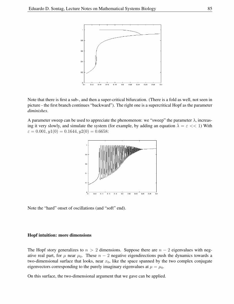
Eduardo D. Sontag, Lecture Notes on Mathematical Systems Biology 85
Note that there is first a sub-, and then a super-critical bifurcation. (There is a fold as well, not seen inpicture - the first branch continues “backward”). The right one is a supercritical Hopf as the parameterdiminishes.
A parameter sweep can be used to appreciate the phenomenon: we “sweep” the parameter λ, increas-ing it very slowly, and simulate the system (for example, by adding an equation λ = ε << 1) Withε = 0.001, y1(0) = 0.1644, y2(0) = 0.6658:
Note the “hard” onset of oscillations (and “soft” end).
Hopf intuition: more dimensions
The Hopf story generalizes to n > 2 dimensions. Suppose there are n − 2 eigenvalues with neg-ative real part, for µ near µ0. These n − 2 negative eigendirections push the dynamics towards atwo-dimensional surface that looks, near x0, like the space spanned by the two complex conjugateeigenvectors corresponding to the purely imaginary eigenvalues at µ = µ0.
On this surface, the two-dimensional argument that we gave can be applied.
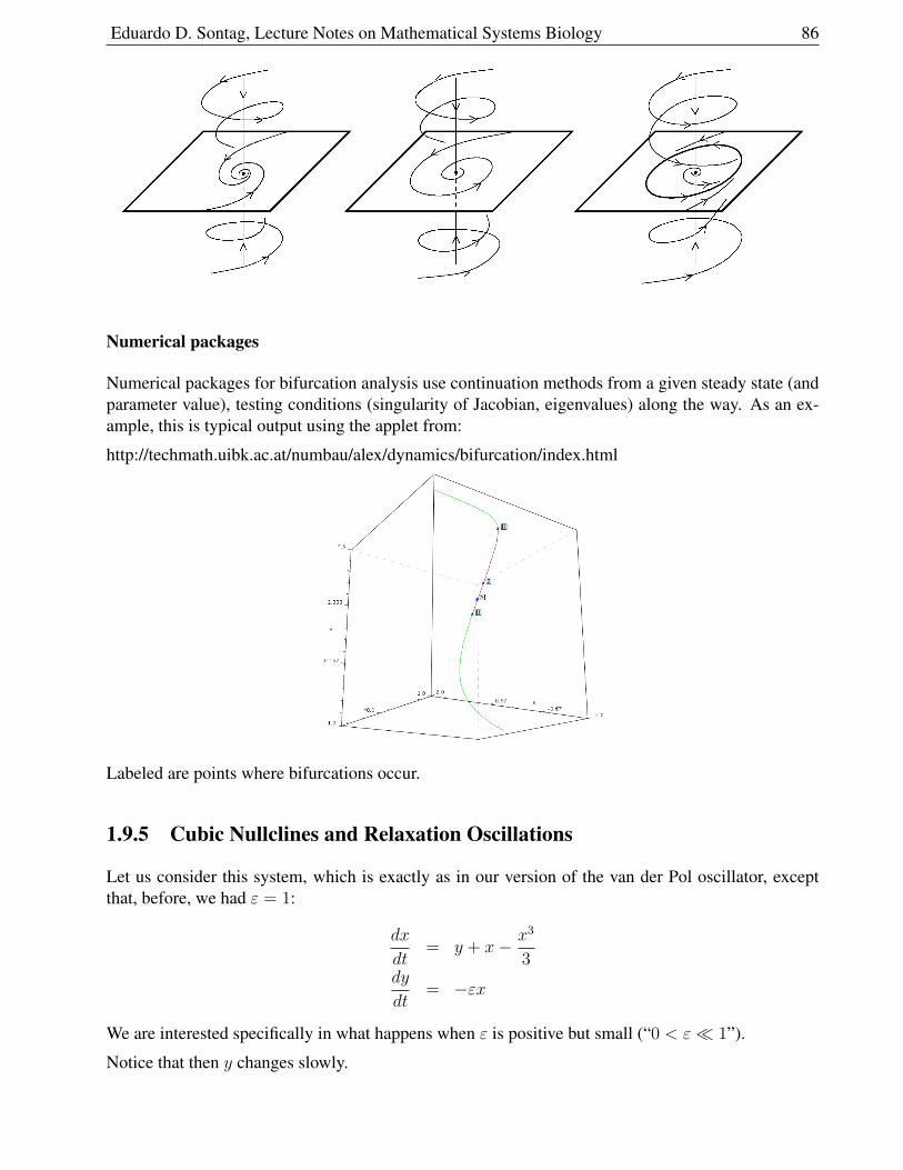
Eduardo D. Sontag, Lecture Notes on Mathematical Systems Biology 86
Numerical packages
Numerical packages for bifurcation analysis use continuation methods from a given steady state (andparameter value), testing conditions (singularity of Jacobian, eigenvalues) along the way. As an ex-ample, this is typical output using the applet from:
http://techmath.uibk.ac.at/numbau/alex/dynamics/bifurcation/index.html
Labeled are points where bifurcations occur.
1.9.5 Cubic Nullclines and Relaxation Oscillations
Let us consider this system, which is exactly as in our version of the van der Pol oscillator, exceptthat, before, we had ε = 1:
dx
dt= y + x− x3
3dy
dt= −εx
We are interested specifically in what happens when ε is positive but small (“0 < ε 1”).
Notice that then y changes slowly.
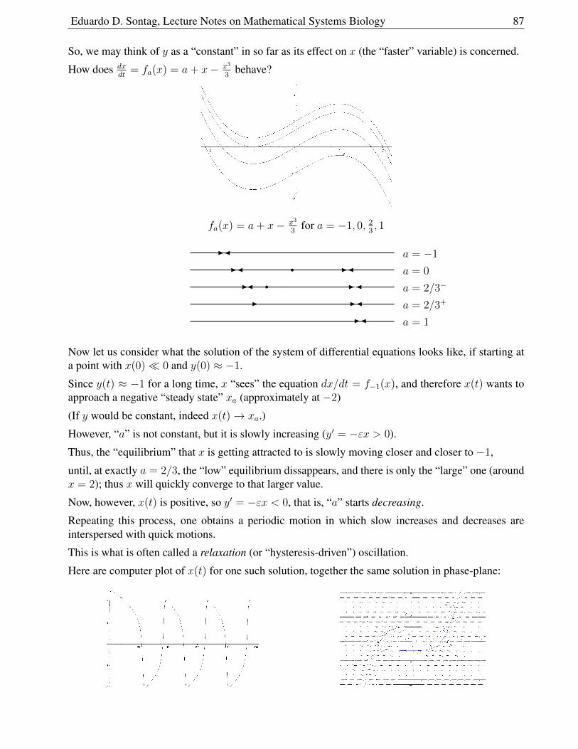
Eduardo D. Sontag, Lecture Notes on Mathematical Systems Biology 87
So, we may think of y as a “constant” in so far as its effect on x (the “faster” variable) is concerned.
How does dxdt
= fa(x) = a+ x− x3
3behave?
fa(x) = a+ x− x3
3for a = −1, 0, 2
3, 1
rr-
- -
- -
- -
-
a = 0
a = −1
a = 2/3−
a = 2/3+
a = 1
Now let us consider what the solution of the system of differential equations looks like, if starting ata point with x(0) 0 and y(0) ≈ −1.
Since y(t) ≈ −1 for a long time, x “sees” the equation dx/dt = f−1(x), and therefore x(t) wants toapproach a negative “steady state” xa (approximately at −2)
(If y would be constant, indeed x(t)→ xa.)
However, “a” is not constant, but it is slowly increasing (y′ = −εx > 0).
Thus, the “equilibrium” that x is getting attracted to is slowly moving closer and closer to −1,
until, at exactly a = 2/3, the “low” equilibrium dissappears, and there is only the “large” one (aroundx = 2); thus x will quickly converge to that larger value.
Now, however, x(t) is positive, so y′ = −εx < 0, that is, “a” starts decreasing.
Repeating this process, one obtains a periodic motion in which slow increases and decreases areinterspersed with quick motions.
This is what is often called a relaxation (or “hysteresis-driven”) oscillation.
Here are computer plot of x(t) for one such solution, together the same solution in phase-plane:
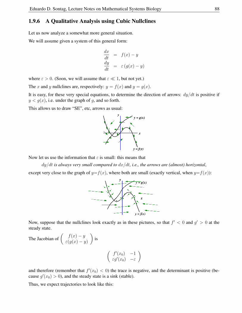
Eduardo D. Sontag, Lecture Notes on Mathematical Systems Biology 88
1.9.6 A Qualitative Analysis using Cubic Nullclines
Let us now analyze a somewhat more general situation.
We will assume given a system of this general form:
dx
dt= f(x)− y
dy
dt= ε (g(x)− y)
where ε > 0. (Soon, we will assume that ε 1, but not yet.)
The x and y nullclines are, respectively: y = f(x) and y = g(x).
It is easy, for these very special equations, to determine the direction of arrows: dy/dt is positive ify < g(x), i.e. under the graph of g, and so forth.
This allows us to draw “SE”, etc, arrows as usual:
Now let us use the information that ε is small: this means that
dy/dt is always very small compared to dx/dt, i.e., the arrows are (almost) horizontal,
except very close to the graph of y=f(x), where both are small (exactly vertical, when y=f(x)):
Now, suppose that the nullclines look exactly as in these pictures, so that f ′ < 0 and g′ > 0 at thesteady state.
The Jacobian of(
f(x)− yε(g(x)− y)
)is
(f ′(x0) −1εg′(x0) −ε
)and therefore (remember that f ′(x0) < 0) the trace is negative, and the determinant is positive (be-cause g′(x0) > 0), and the steady state is a sink (stable).
Thus, we expect trajectories to look like this:
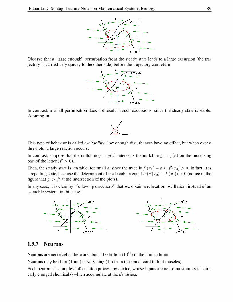
Eduardo D. Sontag, Lecture Notes on Mathematical Systems Biology 89
Observe that a “large enough” perturbation from the steady state leads to a large excursion (the tra-jectory is carried very quicky to the other side) before the trajectory can return.
In contrast, a small perturbation does not result in such excursions, since the steady state is stable.Zooming-in:
This type of behavior is called excitability: low enough disturbances have no effect, but when over athreshold, a large reaction occurs.
In contrast, suppose that the nullcline y = g(x) intersects the nullcline y = f(x) on the increasingpart of the latter (f ′ > 0).
Then, the steady state is unstable, for small ε, since the trace is f ′(x0)− ε ≈ f ′(x0) > 0. In fact, it isa repelling state, because the determinant of the Jacobian equals ε(g′(x0)− f ′(x0)) > 0 (notice in thefigure that g′ > f ′ at the intersection of the plots).
In any case, it is clear by “following directions” that we obtain a relaxation oscillation, instead of anexcitable system, in this case:
1.9.7 Neurons
Neurons are nerve cells; there are about 100 billion (1011) in the human brain.
Neurons may be short (1mm) or very long (1m from the spinal cord to foot muscles).
Each neuron is a complex information processing device, whose inputs are neurotransmitters (electri-cally charged chemicals) which accumulate at the dendrites.
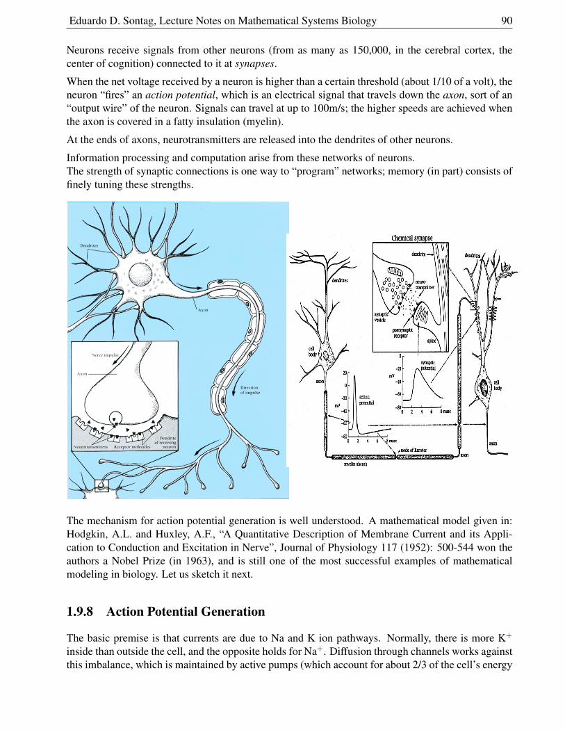
Eduardo D. Sontag, Lecture Notes on Mathematical Systems Biology 90
Neurons receive signals from other neurons (from as many as 150,000, in the cerebral cortex, thecenter of cognition) connected to it at synapses.
When the net voltage received by a neuron is higher than a certain threshold (about 1/10 of a volt), theneuron “fires” an action potential, which is an electrical signal that travels down the axon, sort of an“output wire” of the neuron. Signals can travel at up to 100m/s; the higher speeds are achieved whenthe axon is covered in a fatty insulation (myelin).
At the ends of axons, neurotransmitters are released into the dendrites of other neurons.
Information processing and computation arise from these networks of neurons.The strength of synaptic connections is one way to “program” networks; memory (in part) consists offinely tuning these strengths.
The mechanism for action potential generation is well understood. A mathematical model given in:Hodgkin, A.L. and Huxley, A.F., “A Quantitative Description of Membrane Current and its Appli-cation to Conduction and Excitation in Nerve”, Journal of Physiology 117 (1952): 500-544 won theauthors a Nobel Prize (in 1963), and is still one of the most successful examples of mathematicalmodeling in biology. Let us sketch it next.
1.9.8 Action Potential Generation
The basic premise is that currents are due to Na and K ion pathways. Normally, there is more K+
inside than outside the cell, and the opposite holds for Na+. Diffusion through channels works againstthis imbalance, which is maintained by active pumps (which account for about 2/3 of the cell’s energy
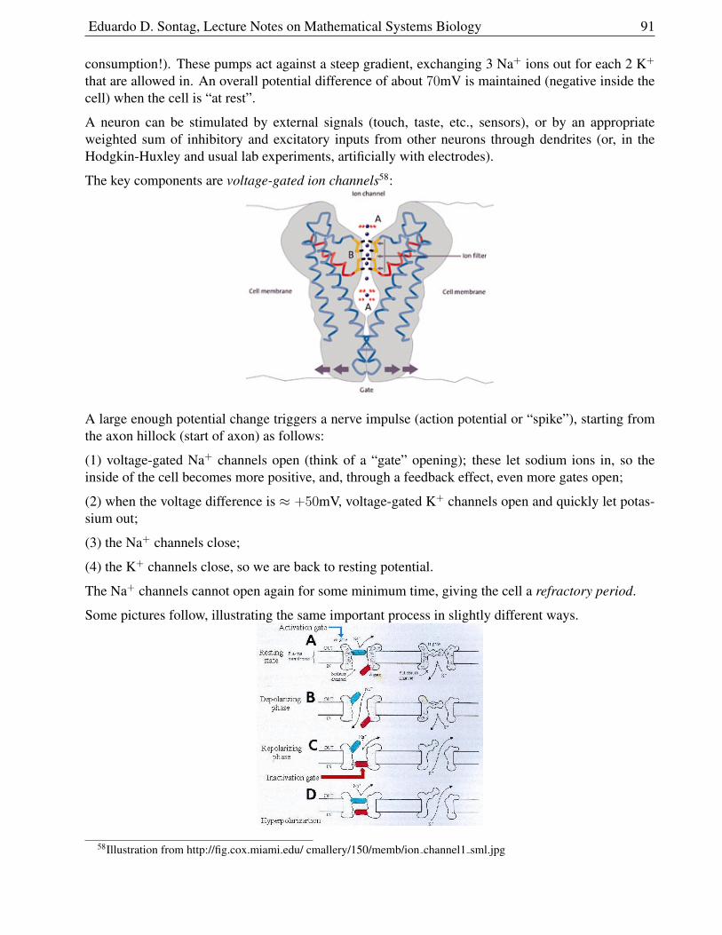
Eduardo D. Sontag, Lecture Notes on Mathematical Systems Biology 91
consumption!). These pumps act against a steep gradient, exchanging 3 Na+ ions out for each 2 K+
that are allowed in. An overall potential difference of about 70mV is maintained (negative inside thecell) when the cell is “at rest”.
A neuron can be stimulated by external signals (touch, taste, etc., sensors), or by an appropriateweighted sum of inhibitory and excitatory inputs from other neurons through dendrites (or, in theHodgkin-Huxley and usual lab experiments, artificially with electrodes).
The key components are voltage-gated ion channels58:
A large enough potential change triggers a nerve impulse (action potential or “spike”), starting fromthe axon hillock (start of axon) as follows:
(1) voltage-gated Na+ channels open (think of a “gate” opening); these let sodium ions in, so theinside of the cell becomes more positive, and, through a feedback effect, even more gates open;
(2) when the voltage difference is ≈ +50mV, voltage-gated K+ channels open and quickly let potas-sium out;
(3) the Na+ channels close;
(4) the K+ channels close, so we are back to resting potential.
The Na+ channels cannot open again for some minimum time, giving the cell a refractory period.
Some pictures follow, illustrating the same important process in slightly different ways.
58Illustration from http://fig.cox.miami.edu/ cmallery/150/memb/ion channel1 sml.jpg
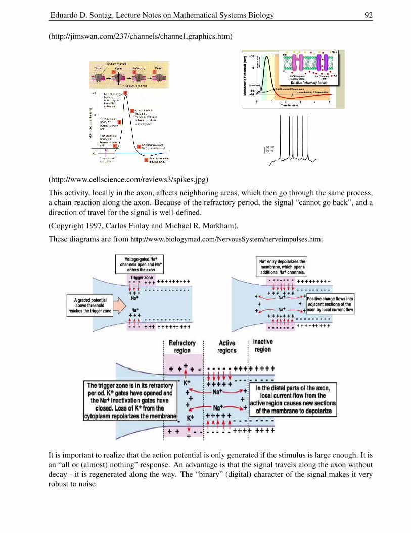
Eduardo D. Sontag, Lecture Notes on Mathematical Systems Biology 92
(http://jimswan.com/237/channels/channel graphics.htm)
(http://www.cellscience.com/reviews3/spikes.jpg)
This activity, locally in the axon, affects neighboring areas, which then go through the same process,a chain-reaction along the axon. Because of the refractory period, the signal “cannot go back”, and adirection of travel for the signal is well-defined.
(Copyright 1997, Carlos Finlay and Michael R. Markham).
These diagrams are from http://www.biologymad.com/NervousSystem/nerveimpulses.htm:
It is important to realize that the action potential is only generated if the stimulus is large enough. It isan “all or (almost) nothing” response. An advantage is that the signal travels along the axon withoutdecay - it is regenerated along the way. The “binary” (digital) character of the signal makes it veryrobust to noise.
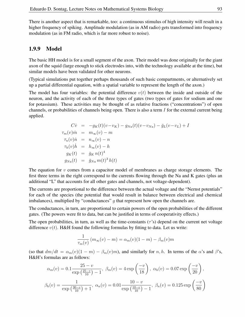
Eduardo D. Sontag, Lecture Notes on Mathematical Systems Biology 93
There is another aspect that is remarkable, too: a continuous stimulus of high intensity will result in ahigher frequency of spiking. Amplitude modulation (as in AM radio) gets transformed into frequencymodulation (as in FM radio, which is far more robust to noise).
1.9.9 Model
The basic HH model is for a small segment of the axon. Their model was done originally for the giantaxon of the squid (large enough to stick electrodes into, with the technology available at the time), butsimilar models have been validated for other neurons.
(Typical simulations put together perhaps thousands of such basic compartments, or alternatively setup a partial differential equation, with a spatial variable to represent the length of the axon.)
The model has four variables: the potential difference v(t) between the inside and outside of theneuron, and the activity of each of the three types of gates (two types of gates for sodium and onefor potassium). These activities may be thought of as relative fractions (“concentrations”) of openchannels, or probabilities of channels being open. There is also a term I for the external current beingapplied.
Cv = −gK(t)(v−vK)− gNa(t)(v−vNa)− gL(v−vL) + I
τm(v)m = m∞(v)−mτn(v)n = n∞(v)− nτh(v)h = h∞(v)− hgK(t) = gK n(t)4
gNa(t) = gNam(t)3 h(t)
The equation for v comes from a capacitor model of membranes as charge storage elements. Thefirst three terms in the right correspond to the currents flowing through the Na and K gates (plus anadditional “L” that accounts for all other gates and channels, not voltage-dependent).
The currents are proportional to the difference between the actual voltage and the “Nernst potentials”for each of the species (the potential that would result in balance between electrical and chemicalimbalances), multiplied by “conductances” g that represent how open the channels are.
The conductances, in turn, are proportional to certain powers of the open probabilities of the differentgates. (The powers were fit to data, but can be justified in terms of cooperativity effects.)
The open probabilities, in turn, as well as the time-constants (τ ’s) depend on the current net voltagedifference v(t). H&H found the following formulas by fitting to data. Let us write:
1
τm(v)(m∞(v)−m) = αm(v)(1−m)− βm(v)m
(so that dm/dt = αm(v)(1 − m) − βm(v)m), and similarly for n, h. In terms of the α’s and β’s,H&H’s formulas are as follows:
αm(v) = 0.125− v
exp(
25−v10
)− 1
, βm(v) = 4 exp
(−v18
), αh(v) = 0.07 exp
(−v20
),
βh(v) =1
exp(
30−v10
)+ 1
, αn(v) = 0.0110− v
exp(
10−v10
)− 1
, βn(v) = 0.125 exp
(−v80
)
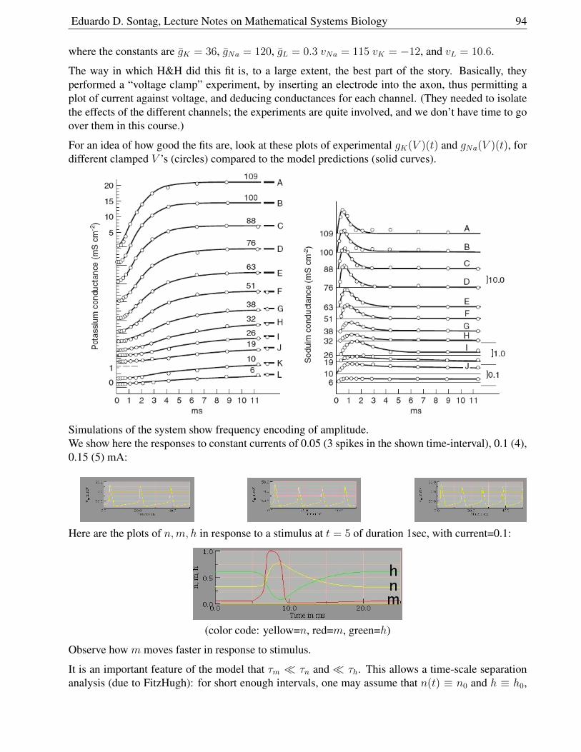
Eduardo D. Sontag, Lecture Notes on Mathematical Systems Biology 94
where the constants are gK = 36, gNa = 120, gL = 0.3 vNa = 115 vK = −12, and vL = 10.6.
The way in which H&H did this fit is, to a large extent, the best part of the story. Basically, theyperformed a “voltage clamp” experiment, by inserting an electrode into the axon, thus permitting aplot of current against voltage, and deducing conductances for each channel. (They needed to isolatethe effects of the different channels; the experiments are quite involved, and we don’t have time to goover them in this course.)
For an idea of how good the fits are, look at these plots of experimental gK(V )(t) and gNa(V )(t), fordifferent clamped V ’s (circles) compared to the model predictions (solid curves).
Simulations of the system show frequency encoding of amplitude.We show here the responses to constant currents of 0.05 (3 spikes in the shown time-interval), 0.1 (4),0.15 (5) mA:
Here are the plots of n,m, h in response to a stimulus at t = 5 of duration 1sec, with current=0.1:
(color code: yellow=n, red=m, green=h)
Observe how m moves faster in response to stimulus.
It is an important feature of the model that τm τn and τh. This allows a time-scale separationanalysis (due to FitzHugh): for short enough intervals, one may assume that n(t) ≡ n0 and h ≡ h0,
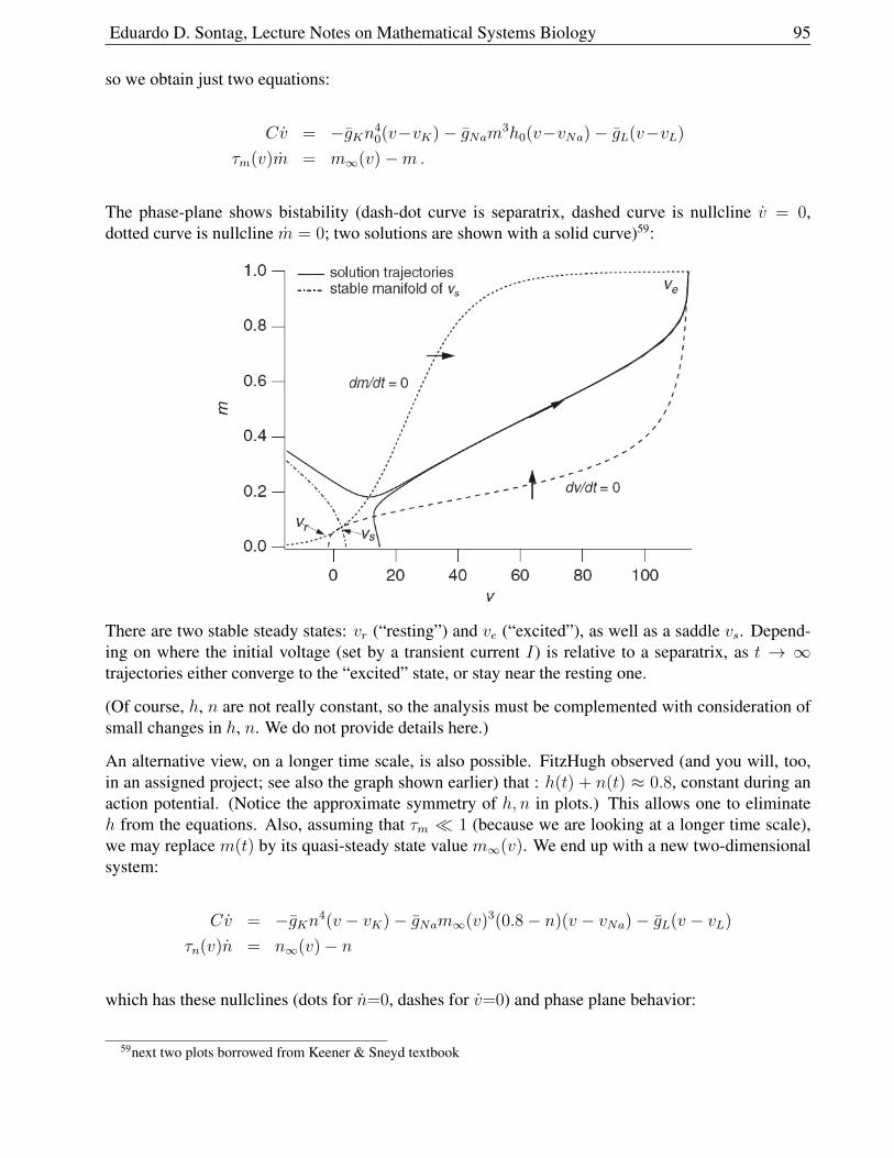
Eduardo D. Sontag, Lecture Notes on Mathematical Systems Biology 95
so we obtain just two equations:
Cv = −gKn40(v−vK)− gNam3h0(v−vNa)− gL(v−vL)
τm(v)m = m∞(v)−m.
The phase-plane shows bistability (dash-dot curve is separatrix, dashed curve is nullcline v = 0,dotted curve is nullcline m = 0; two solutions are shown with a solid curve)59:
There are two stable steady states: vr (“resting”) and ve (“excited”), as well as a saddle vs. Depend-ing on where the initial voltage (set by a transient current I) is relative to a separatrix, as t → ∞trajectories either converge to the “excited” state, or stay near the resting one.
(Of course, h, n are not really constant, so the analysis must be complemented with consideration ofsmall changes in h, n. We do not provide details here.)
An alternative view, on a longer time scale, is also possible. FitzHugh observed (and you will, too,in an assigned project; see also the graph shown earlier) that : h(t) + n(t) ≈ 0.8, constant during anaction potential. (Notice the approximate symmetry of h, n in plots.) This allows one to eliminateh from the equations. Also, assuming that τm 1 (because we are looking at a longer time scale),we may replace m(t) by its quasi-steady state value m∞(v). We end up with a new two-dimensionalsystem:
Cv = −gKn4(v − vK)− gNam∞(v)3(0.8− n)(v − vNa)− gL(v − vL)
τn(v)n = n∞(v)− n
which has these nullclines (dots for n=0, dashes for v=0) and phase plane behavior:
59next two plots borrowed from Keener & Sneyd textbook
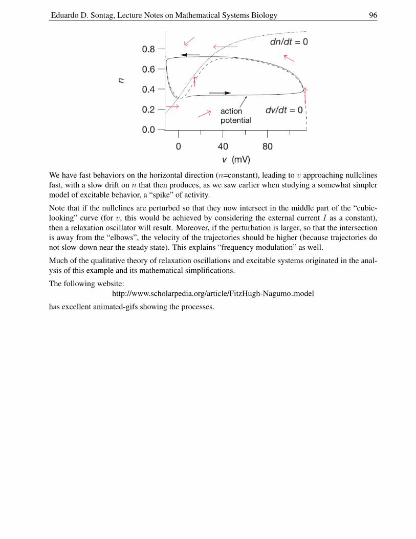
Eduardo D. Sontag, Lecture Notes on Mathematical Systems Biology 96
We have fast behaviors on the horizontal direction (n=constant), leading to v approaching nullclinesfast, with a slow drift on n that then produces, as we saw earlier when studying a somewhat simplermodel of excitable behavior, a “spike” of activity.
Note that if the nullclines are perturbed so that they now intersect in the middle part of the “cubic-looking” curve (for v, this would be achieved by considering the external current I as a constant),then a relaxation oscillator will result. Moreover, if the perturbation is larger, so that the intersectionis away from the “elbows”, the velocity of the trajectories should be higher (because trajectories donot slow-down near the steady state). This explains “frequency modulation” as well.
Much of the qualitative theory of relaxation oscillations and excitable systems originated in the anal-ysis of this example and its mathematical simplifications.
The following website:http://www.scholarpedia.org/article/FitzHugh-Nagumo model
has excellent animated-gifs showing the processes.
Eduardo D. Sontag, Lecture Notes on Mathematical Systems Biology 97
1.10 Problems for ODE chapter
1.10.1 Population growth
1. Show that the solution of the logistic equation, given by N(t) = N0BN0+(B−N0)e−rt
, has the follow-ing properties:
(a) N → B as t→∞.
(b) The graph of N(t) is concave up for N0 < N < B2
when N0 < B. [Hint: calculate d2Ndt2
.]
(c) The graph of N(t) is concave down for B2< N < B when N0 < B.
(d) The graph ofN(t) is concave up whenN0 > B. Provide a rough plot of the graph, assumingthat N0 > B.
2. Sometimes, with large populations competing for limited resources, this competition mightresult in struggles that prevent reproduction, so that dN
dt(t) is actually smaller if N(t) is larger.
(Another example is tumor cells that have less access to blood vessels when the volume of thetumor is large.) This means that d2N
dt2< 0 if N is large, and is sometimes called “decelerating
growth for large populations” (“decreasing growth” would be a more accurate term!), thoughother authors may use that term with a slightly different meaning.60
(i) Show that, if N is a solution of dNdt
(t) = f(N(t)), then d2Ndt2
(t) = f ′(N(t))f(N(t))
Thus, in order to test decelerating growth, we need to test f ′(N)f(N) < 0 when N is large.
Let us may write single population models as dNdt
= K(N)N , where we think of K(N) as a“per capita” growth rate. In the simplest exponential growth model, K(N) is constant, and inthe logistic model, K(N) is a linear function. But many other choices are possible as well. Forsingle-species populations, consider the following per-capita growth rates K(N), and answerfor which of them we have decelerating growth:
(a) K(N) = β1+N
, β > 0.
(b) K(N) = β −N, β > 0.
(c) K(N) = N − eαN , α > 0.
(d) K(N) = logN .
(e) Which of the above growth rates would result in a stable population size?
(f) Think of examples in biology where these different growth rates may arise.
3. The “Allee effect” in biology (named after American zoologist and ecologist Warder ClydeAllee) is that in which there is a positive correlation between population density and the percapita population growth rate K(N) in very small populations. In Allee-effect models, thefunction K(N) has a strict maximum at some intermediate value α of density, on the interval[0, B]:
dK/dN > 0 for 0 < N < α , dK/dN < 0 for α < N < B
60For example, search in Google books inside the book “Cancer of the breast” by William L. Donegan and John StricklinSpratt, or the paper “Decelerating growth and human breast cancer” by John A. Spratt, D. von Fournier, John S. Spratt,and Ernst E. Weber, Cancer, Volume 71, pages 20132019, March 1993.
Eduardo D. Sontag, Lecture Notes on Mathematical Systems Biology 98
(and K(B) = 0). Such a model applies when there is a carrying capacity, limiting growthat large densities, as in the logistic model, but also growth is impeded at low densities (forexample, because of the difficulty in finding mates at low densities).
(a) Give an explicit example of a parabola K(N) that has these properties.
(b) Sketch a plot of any function K(N) that satisfies these properties.
(c) Sketch a plot K(N)N .
(d) What are the stable points of dN/dt = K(N)N , for such a function K(N)?
4. The continuous-time Beverton-Holt population growth model in fisheries is:
dN
dt=
rN
α +N
(Beverton and Holt, 1957; Keshet’s book).
(a) Find k1 and k2 so that, with N∗ = k1N and t∗ = k2t, we obtain the following “dimension-less” form of the Beverton-Holt model:
dN∗
dt∗=
N∗
1 +N∗.
(b) Analyze the behavior of the solutions to this equation.
5. Another population growth model used in fisheries is the continuous Ricker model:
dN
dt= rNe−βN
(Ricker, 1954; Keshet’s book). (a) Find k1 and k2 so that, with N∗ = k1N and t∗ = k2t, weobtain the following “dimensionless” form of the Ricker model:
dN∗
dt∗= N∗e−N
∗.
(b) Analyze the behavior of the solutions to this equation.
1.10.2 Interacting population problems
When species interact, the population dynamics of each species is affected.There are three main types of interactions:
• If the growth rate of one of the populations is decreased, and the other increased, the populationsare in a predator-prey relationship.
• If the growth rate of each population is decreased, then they are in a competition relationship.
• If each population’s growth rate is enhanced, then they are in a mutualism relationship.
Eduardo D. Sontag, Lecture Notes on Mathematical Systems Biology 99
1. (Predator-Prey Models) The classical version of the Lotka-Volterra predator-prey system is asfollows:
dN
dt= N(a− bP )
dP
dt= P (cN − d) .
Here, N(t) is the prey population and P (t) is the predator population at time t, and a, b, c andd are positive constants.
(a) Briefly explain the ecological assumptions in the model, i.e. interpret each term in theequations.
(b) Find a rescaling of variables that makes the model have as few parameters as possible.
(c) Determine the steady states and their stability.
(d)(i) Show that the solution of the differential equation with d = a and initial conditionsN(0) = 2 and P (0) = 1
2satisfies:
N(t) + P (t)− log (N(t)P (t)) =5
2(∗)
for all t ≥ 0. (Hint: show that the derivative of N(t) + P (t)− log (N(t)P (t)) is zero.)
(ii) Plot the solutions of N(t) + P (t)− log (N(t)P (t)) = 52. Are the solutions periodic?
(iii) Give a general formula like (∗) for arbitrary a, b, c, d, and any initial conditions.
2. (Predator-prey model with limited growth.) Here is a modified version of the classical versionof the predator-prey model, in which there is logistic growth for the prey, with carrying capacityK, as follows:
dN
dt= α
(1− N
K
)N − γPN = αN − βN2 − γPN
dP
dt= −δP + εPN .
We have that β = α/K and α now represents the inherent per capita net growth rate for theprey in the absence of predators. As in the previous predator-prey model, preadtors eat onlyprey, and, if there were no prey, they would die at a constant per capita rate.
(a) Draw the nullclines of the system. Under what condition there is a non-trivial intersection?
(b) Show that the steady states for the model are (0, 0),(αβ, 0)
, and(δ
ε,α
γ− βδ
γε
).
(c) Form the Jacobian matrix at(δε, αγ− βδ
γε
). Show that
(δε, αγ− βδ
γε
)is a stable steady state.
3. (Another revised predator-prey model.) This example illustrates how the type of equilibriummay change because of changes in the values of the model parameters.
Eduardo D. Sontag, Lecture Notes on Mathematical Systems Biology 100
As in the previous model, we have predators P and prey voles N. The prey growth follows thelogistic equation as in the predator-prey model with limited growth, but we change the growthassumption regarding predators : instead of being proportional toNP , it is proportional to NP
1+N,
a Michaelis-Menten rate:dN
dt= αN − βN2 − γ PN
1 +N
We also change the assumptions on the predator growth rate:
dP
dt= δP
(1− εP
N
)reflecting a carrying capacity proportional to the prey population. Consider this system, withthe parameters α = 2
3, β = 1
6, γ = 1, and ε = 1 and answer the following questions.
(a) Draw the nullclines. Make sure to show the directions of movement for the model.
(b) Show that A = (1, 1) is a steady state. Under what condition A is stable and under whatcondition A is an unstable steady state?
4. (Competition Models) We now consider the basic two-species Lotka-Volterra competitionmodel with each species N1 and N2 having logistic growth in the absence of the other:
dN1
dt= r1N1
[1− N1
k1
− b12N2
k1
]dN2
dt= r2N2
[1− N2
k2
− b21N1
k2
]where r1, r2, k1, k2, b12 and b21 are all positive constants, the r’s are the linear birth rates, andthe k’s are the carrying capacities. The constants b12 and b21 measure the competitive effect ofN2 on N1 and N1 on N2 respectively.
(a) Find a rescaling of variables that makes the model have as few parameters as possible.
(i) Show that (0, 0) is unstable.
(ii) Show that (1, 0) is stable if b21k1 > k2 and unstable if b21k1 < k2.
(iii) Under what conditions can you guarantee that (0, 1) is stable or unstable?
(b) In the special case that b12b21 = 1, show that there are three steady states (0, 0), (1, 0), and(0, 1).
(i) Show that (0, 0) is unstable.
(ii) Show that (1, 0) is stable if b21k1 > k2 and unstable if b21k1 < k2.
(iii) Under what conditions can you guarantee that (0, 1) is stable or unstable?
(c) (i) Show that there are four steady states when k1 = k2 and b12 = b21 = 12, and there is a
steady state with both N − 1 > 0 and N2 > 0 which is stable (a coexistence state).
(ii) Sketch the N1-nullcline and N2-nullcline of the system in part (i).
(d) (i) Show that there are four steady states when k1 = k2 and b12 = b21 = 2, and there is asteady state with both N1 > 0 and N2 > 0 which is a saddle.
(ii) Sketch the N1-nullcline and N2-nullcline of the system in part (i).
Eduardo D. Sontag, Lecture Notes on Mathematical Systems Biology 101
5. (Mutualism or Symbiosis Models) There are many examples that show the interaction of twoor more species has advantages for all. Mutualism often plays the crucial role in promotingand even maintaining such species: plant and seed dispersal is one example. The simplestmutualism model analogous to the classical Lotka-Volterra predator-prey one is as follows:
dN1
dt= r1N1 + a1N1N2
dN2
dt= r2N2 + a2N2N1
where r1, r2, a1 and a2 are all positive constants.
Determine the steady states and their stabilities.
6. (a) Determine the kind of interactive behavior between two species with populations N1 and N2
that is implied by the following model:
dN1
dt= r1N1
(1− N1
k1 + b12N2
)dN2
dt= r2N2
(1− N2
k2 + b21N1
)where r1, r2, k1, k2, b12 and b21 are all positive constants.
(b) Find a rescaling of variables that makes the model have as few parameters as possible.
(c) Determine the steady states of the system and their stabilities.
(d) Draw the nullclines of the system.
7. (a) Determine the kind of interactive behavior between two species with populations N1 and N2
that is implied by the following model:
dN1
dt= rN1
(1− N1
k
)− aN1N2 (1− exp(−bN1))
dN2
dt= −dN2 +N2e (1− exp(−bN1))
where r, a, b, d, e and k are positive constants.
(b) Find a rescaling of variables that makes the model have as few parameters as possible.
(c) Determine the steady states of the system and their stabilities.
(d) Draw the nullclines of the system.
8. (a) Determine the kind of interactive behavior between two species with populations N1 and N2
that is implied by the following model:
dN1
dt= N1(a− d(N1 +N2)− b)
dN2
dt= N2(a− d(N1 +N2)− sb)
where a, b, d are positive constants and s < 1 is a measure of the difference in mortality of thetwo species.
Eduardo D. Sontag, Lecture Notes on Mathematical Systems Biology 102
(b) Find a rescaling of variables that makes the model have as few parameters as possible.
(c) Show that the population N1 and N2 are related by:
N1(t) = cN2(t)e(s−1)t
for a constant c.
(d) Determine the steady states of the system and their stabilities.
(e) Draw the nullclines of the system.
1.10.3 Chemostat problems
1. For the chemostat model, analyze stability of X1 when the parameters are chosen such that theequilibrium X2 does not exist.
2. Suppose that we have built a chemostat and we model it as usual, with a Michaelis-Mentengrowth rate. Moreover, we have measured all constants and, in appropriate units, have:
V = 2 and kmax = α = F = kn = 1 .
What should the concentration of the nutrient in the supply tank be, so that the steady stateconcentration of bacteria is exactly 20? (Don’t worry about units. Assume that all units arecompatible.)
Answering this question should only take a couple of lines. You may use any formula from thenotes that you want to.
3. Suppose that we use a Michaelis-Menten growth rate in the chemostat model, and that theparameters are chosen so that a positive steady state exists.
(a) Show that
N = f(V, F, C0) =C0(F − V Km) + FKn
α (F − V Km)
andC =
FKn
F − V Km
at the positive steady state.
(b) Show that either of these: (a) increasing the volume of the culture chamber, (b) increasingthe concentration of nutrient in the supply tank, or (3) decreasing the flow rate, provides away to increase the steady-state value of the bacterial population. (Hint: compute partialderivatives.)
4. Suppose that we use K(C) = kC (for some constant k) instead of a Michaelis-Menten growthrate, in the chemostat model.
(a) Find a change of variables so that only one parameter remains.
(b) Find the steady state(s). Express it (them) in terms of the original parameters. Determineconditions on parameters so that a positive steady state exists, and explain intuitively whythese conditions make sense.
Eduardo D. Sontag, Lecture Notes on Mathematical Systems Biology 103
(c) Compare the conditions you just obtained with the ones that we got in the MM case.
(d) Determine the stability of the positive steady state, if it exists.
5. This is purely a modeling problem (there is no one “correct” answer!). We ask about ways togeneralize the chemostat - just provide sets of equations, no need to solve anything.
(a) How would you change the model to allow for two growth-limiting nutrients? NowK(C1, C2), the rate of reproduction per unit time, depends on two concentrations.61 Itis a little harder to write how the nutrients are being consumed in this multiple nutrientcase. Think about this and be creative.62
(b) Suppose that at high densities the microorganism secretes a chemical that inhibits growth.How would you model that?
(c) Model the case when two types of microorganisms compete for the same nutrient.
6. This is yet another variation on the chemostat. Suppose that there is a membrane that filters theoutflow, so that the microorganism never flows out (only the nutrient does). Assume, however,that the microorganism dies at a certain rate µN .
(a) Write down a model, assuming K(C) is Michaelis-Menten.
(b) Find a change of variables that leads to a system with three parameters as follows:
dN
dt= α1(
C
C + 1)N − α3N
dC
dt= −(
C
C + 1)N − C + α2
(c) Show that there are two steady states, one with N = 0. Show that the second one haspositive coordinates provided that:
α1 > α3 & α2 −α3
α1 − α3
> 0 ,
(d) Show that this second equilibrium is always stable (if it has positive coordinates).
7. Consider this system of equations (which corresponds to a chemostat with K(C) = C):
dN
dt= CN −N
dC
dt= −CN − C + 5 .
The sketch below has the nullclines (there are vertical arrows on the C axis too).
61One possibility if to use K(C1, C2) = maxK1(C1),K2(C2), in the case in which the bacteria decide to use thenutrient that is in most abundance preferentially (this actually happens with certain sugar consumptions - a beautiful ex-ample of bacterial computation; search “lac operon” on the web). Another would be to takeK as some linear combinationof C1 and C2, etc. What is the least that one should assume about K, though?
62It is amusing to see can be found by typing “multiple nutrients chemostat” into Google (you might recognize some ofthe authors of the first paper that comes up :).
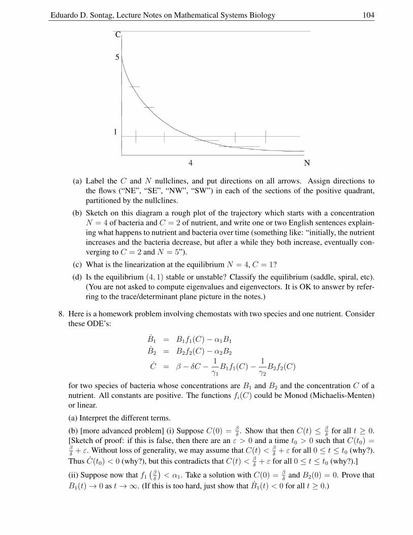
Eduardo D. Sontag, Lecture Notes on Mathematical Systems Biology 104
(a) Label the C and N nullclines, and put directions on all arrows. Assign directions tothe flows (“NE”, “SE”, “NW”, “SW”) in each of the sections of the positive quadrant,partitioned by the nullclines.
(b) Sketch on this diagram a rough plot of the trajectory which starts with a concentrationN = 4 of bacteria and C = 2 of nutrient, and write one or two English sentences explain-ing what happens to nutrient and bacteria over time (something like: “initially, the nutrientincreases and the bacteria decrease, but after a while they both increase, eventually con-verging to C = 2 and N = 5”).
(c) What is the linearization at the equilibrium N = 4, C = 1?
(d) Is the equilibrium (4, 1) stable or unstable? Classify the equilibrium (saddle, spiral, etc).(You are not asked to compute eigenvalues and eigenvectors. It is OK to answer by refer-ring to the trace/determinant plane picture in the notes.)
8. Here is a homework problem involving chemostats with two species and one nutrient. Considerthese ODE’s:
B1 = B1f1(C)− α1B1
B2 = B2f2(C)− α2B2
C = β − δC − 1
γ1
B1f1(C)− 1
γ2
B2f2(C)
for two species of bacteria whose concentrations are B1 and B2 and the concentration C of anutrient. All constants are positive. The functions fi(C) could be Monod (Michaelis-Menten)or linear.
(a) Interpret the different terms.
(b) [more advanced problem] (i) Suppose C(0) = βδ. Show that then C(t) ≤ β
δfor all t ≥ 0.
[Sketch of proof: if this is false, then there are an ε > 0 and a time t0 > 0 such that C(t0) =βδ
+ ε. Without loss of generality, we may assume that C(t) < βδ
+ ε for all 0 ≤ t ≤ t0 (why?).Thus C(t0) < 0 (why?), but this contradicts that C(t) < β
δ+ ε for all 0 ≤ t ≤ t0 (why?).]
(ii) Suppose now that f1
(βδ
)< α1. Take a solution with C(0) = β
δand B2(0) = 0. Prove that
B1(t)→ 0 as t→∞. (If this is too hard, just show that B1(t) < 0 for all t ≥ 0.)
Eduardo D. Sontag, Lecture Notes on Mathematical Systems Biology 105
This says that the first type of bacteria will become extinct, even if there are no bacteria ofthe second type. So, from now on we assume that f1
(βδ
)> α1, and for the same reason,
f2
(βδ
)> α2. Consider these two numbers λi, the “break-even concentrations”:
fi(λi) = αi .
Let us pick the smallest of the two; let us say that λ1 < λ2 (the other case is entirely analogous).The following theorem is the “competitive exclusion principle” for chemostats:
Theorem: Unless B1(0) = 0, one has that B2(t) → 0 as t → ∞ and B1(t) converges to anonzero steady state, which it is easy to see must be γ1
α1(β − δλ1).
This is neat. It says that the bacterium with the smallest requirements completely wins thecompetition. No co-existence! (The equilibrium with B1 = 0 and B2 = γ2
α2(β − δλ2) is
unstable.) There are different theorems that apply to different types of functions fi; in particularone by Hsu (1978) for Michaelis-Menten and one by Wolkowicz and Lu (1992) for linear fi’s; anice summary is given in “Competition in the chemostat: Some remarks”, by P. De Leenheer, B.Li, and H.L. Smith, Canadian Applied Mathematics Quarterly 11(2003): 229-248 (the theoremis valid more generally for N > 2 species as well).
(c) Consider specifically this system:
B1 = B1C −B1
B2 = B2C − 2B2
C = 3− C − 1
2B1C −
1
2B2C .
(i) Find the equilibrium points of this system. Compute the break-even concentrations λ1 andλ2.
(ii) In particular, there will be two equilibria of the forms: X1 = (b1, 0, c1) and X2 = (0, b2, c2).Which of the two should be stable, according to the theory?
(iii) Compute the Jacobians at X1 and X2 and find the eigenvalues (use a computer if wanted).Show that all eigenvalues at X1 are real and negative, but at X2 there is a real positive eigen-value.
(d) Suppose that we pick fi(C) = C as in (c)(iii), but we now have arbitrary parameters αi, etc.satisfying fi
(βδ
)> αi.
(i) Compute the equilibria X1 = (b1, 0, c1) and X2 = (0, b2, c2).
(ii) Under what conditions on the parameters does the theory predict that X2 will be stable?
(iii) Assuming the conditions in (ii), show that the linearized matrix at X2 is stable and at X1 isunstable.
9. Consider the steady states of the chemostat, as found in Section 1.2.1. In pharmaceutical andother applications, one wishes to maximize the yield of bacteria at steady state, N1. How wouldyou pick values of V , F , C0 to make this yield large?
10. In Section 1.1.10, we reduced the number of parameters in the chemostat by using t = VF
,
C = kn, and N =knF
αV kmax. Let us now make a different choice for C and t (leaving N the
same), as follows:
t =1
kmax, C =
FC0
kmaxV.
Eduardo D. Sontag, Lecture Notes on Mathematical Systems Biology 106
(a) Find the transformed form of the system and group the parameters into two new constants.
(b) Write the stability conditions for the chemostat in terms of the new constants.
(c) Show that X1 is stable only when X2 is not.
11. For the standard chemostat with Michaelis-Menten kinetics, we found that one condition forthe second steady state to be positive was that: kmax > F
V.
(a) Prove that, if instead kmax < FV
, then dN/dt < 0, which means that bacteria will becomeextinct (no matter how much nutrient there is!).
(b) Interpret the second condition, C0 >kn
VFkmax−1
.
1.10.4 Chemotherapy and other metabolism and drug infusion problems
1. Consider the chemotherapy model (section “Effect of Drug on Cells in an Organ”). Supposethat K(C) is Michaelis-Menten.
(a) Show how to reduce the model to having just three constants.
(b) There are again two steady states, one with N = 0. Find conditions under which thereis a second one that has positive coordinates. Interpret biologically what your conditionsmean.
(c) In contrast to the chemostat (where the objective is to get the microorganisms to grow),it would be desirable if the equilibrium with N = 0 is stable and the second one eitherdoesn’t exist (in the positive quadrant) or is unstable. Why would a stable second equilib-rium be bad? (Just one sentence, please.)
(d) Find conditions guaranteeing that the equilibrium with N = 0 is stable and show that, un-der these conditions, the second equilibrium, if it is in the first quadrant, must be unstable.
2. For the chemotherapy model discussed above, write a computer program in your favorite pack-age (MATLAB, Mathematica, Maple, whatever) to simulate it (or use “Jode”), and plot solu-tions from several different initial conditions (show N(t) and C(t) versus t on the same plot,using different line styles such as lines and dots or dashes or different colors). Do so for setsof parameters that illustrate a few of the possible cases (second equilibrium exists as a positivesolution or now; equilibrium with N = 0 is stable or not)
3. For the chemotherapy model discussed above, and assuming that parameters are so that theequilibrium with N = 0 is stable and the one in the positive orthant is unstable, there are twopossibilities: (a) all solutions (except for a set of measure zero of initial conditions) converge tothe equilibrium with N = 0 is stable; (b) there is set of initial conditions with nonzero measurefor which solutions do not converge to the equilibrium with N = 0. Determine which is thecase, and prove your conclusions rigorously. (Some numerical experimentation will be useful,of course.)
4. We base this problem on the following paper:
M.B. Rabinowitz, G.W. Wetherill, and J.D. Kopple, “Lead metabolism in the normal human:stable isotope studies,” in Science, vol. 182, 1973, pp. 725 - 727.
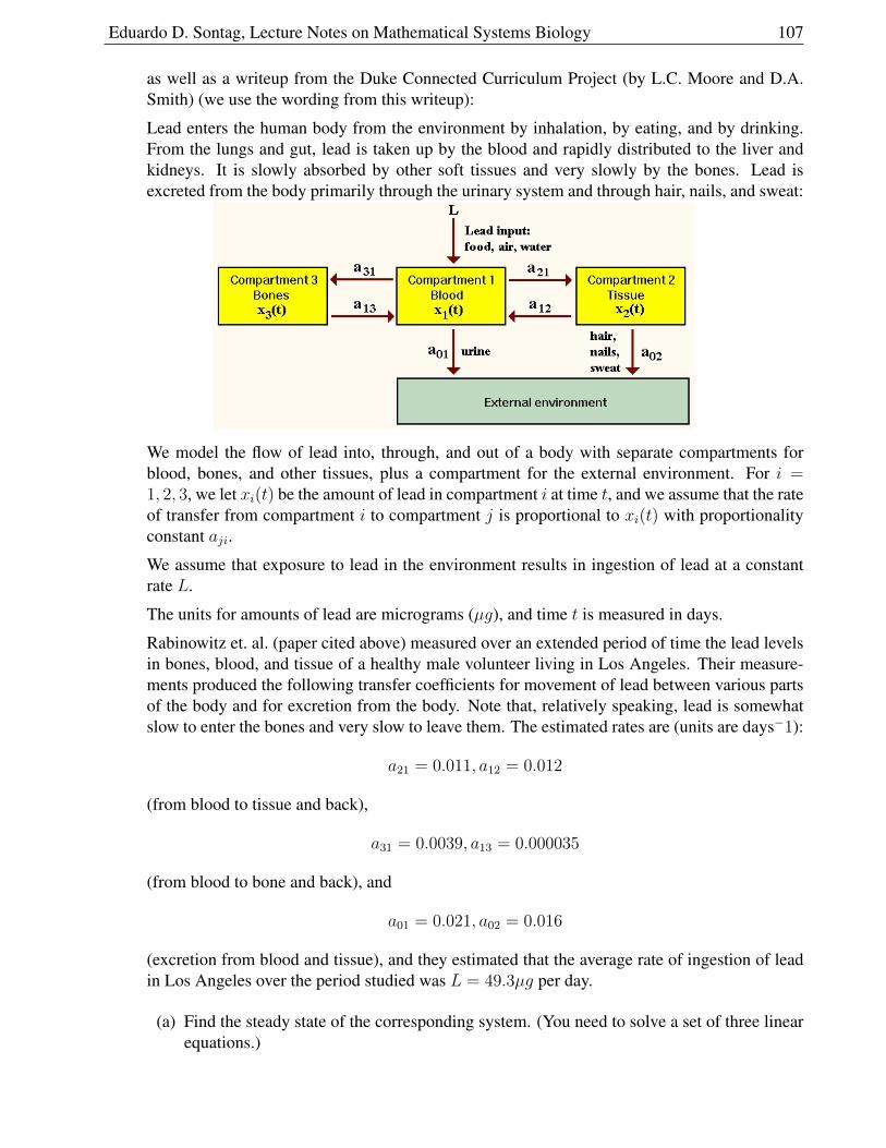
Eduardo D. Sontag, Lecture Notes on Mathematical Systems Biology 107
as well as a writeup from the Duke Connected Curriculum Project (by L.C. Moore and D.A.Smith) (we use the wording from this writeup):
Lead enters the human body from the environment by inhalation, by eating, and by drinking.From the lungs and gut, lead is taken up by the blood and rapidly distributed to the liver andkidneys. It is slowly absorbed by other soft tissues and very slowly by the bones. Lead isexcreted from the body primarily through the urinary system and through hair, nails, and sweat:
We model the flow of lead into, through, and out of a body with separate compartments forblood, bones, and other tissues, plus a compartment for the external environment. For i =1, 2, 3, we let xi(t) be the amount of lead in compartment i at time t, and we assume that the rateof transfer from compartment i to compartment j is proportional to xi(t) with proportionalityconstant aji.
We assume that exposure to lead in the environment results in ingestion of lead at a constantrate L.
The units for amounts of lead are micrograms (µg), and time t is measured in days.
Rabinowitz et. al. (paper cited above) measured over an extended period of time the lead levelsin bones, blood, and tissue of a healthy male volunteer living in Los Angeles. Their measure-ments produced the following transfer coefficients for movement of lead between various partsof the body and for excretion from the body. Note that, relatively speaking, lead is somewhatslow to enter the bones and very slow to leave them. The estimated rates are (units are days−1):
a21 = 0.011, a12 = 0.012
(from blood to tissue and back),
a31 = 0.0039, a13 = 0.000035
(from blood to bone and back), and
a01 = 0.021, a02 = 0.016
(excretion from blood and tissue), and they estimated that the average rate of ingestion of leadin Los Angeles over the period studied was L = 49.3µg per day.
(a) Find the steady state of the corresponding system. (You need to solve a set of three linearequations.)
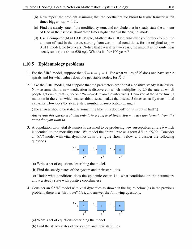
Eduardo D. Sontag, Lecture Notes on Mathematical Systems Biology 108
(b) Now repeat the problem assuming that the coefficient for blood to tissue transfer is tentimes bigger: a21 = 0.11.
(c) Find the steady state of the modified system, and conclude that in steady state the amountof lead in the tissue is about three times higher than in the original model.
(d) Use a computer (MATLAB, Maple, Mathematica, JOde, whatever you prefer) to plot theamount of lead in the tissue, starting from zero initial conditions, for the original (a21 =0.011) model, for two years. Notice that even after two years, the amount is not quite nearsteady state (it is about 620 µg). What is it after 100 years?
1.10.5 Epidemiology problems
1. For the SIRS model, suppose that β = ν = γ = 1. For what values of N does one have stablespirals and for what values does one get stable nodes, for X2?
2. Take the SIRS model, and suppose that the parameters are so that a positive steady state exists.Now assume that a new medication is discovered, which multiplies by 20 the rate at whichpeople get cured (that is, become “removed” from the infectives). However, at the same time, amutation in the virus which causes this disease makes the disease 5 times as easily transmittedas earlier. How does the steady state number of susceptibles change?
(The answer should be stated as something like “it is doubled” or “it is cut in half”.)
Answering this question should only take a couple of lines. You may use any formula from thenotes that you want to.
3. A population with vital dynamics is assumed to be producing new susceptibles at rate δ whichis identical to the mortality rate. We model the “birth” rate as a term δN in dS/dt. Consideran SIR model with vital dynamics as in the figure shown below, and answer the followingquestions.
(a) Write a set of equations describing the model.
(b) Find the steady states of the system and their stabilities.
(c) Under what conditions does the epidemic occur, i.e., what conditions on the parametersallow a steady state with positive coordinates?
4. Consider an SIRS model with vital dynamics as shown in the figure below (as in the previousproblem, there is a “birth rate” δN ), and answer the following questions.
(a) Write a set of equations describing the model.
(b) Find the steady states of the system and their stabilities.
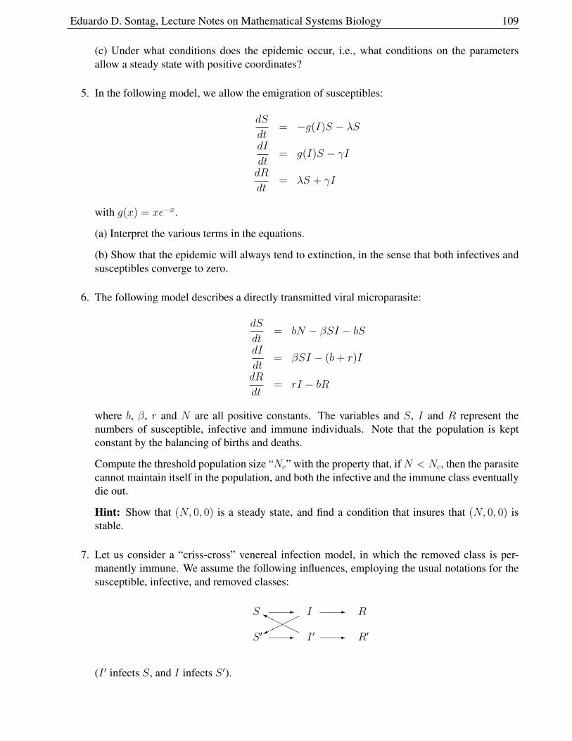
Eduardo D. Sontag, Lecture Notes on Mathematical Systems Biology 109
(c) Under what conditions does the epidemic occur, i.e., what conditions on the parametersallow a steady state with positive coordinates?
5. In the following model, we allow the emigration of susceptibles:
dS
dt= −g(I)S − λS
dI
dt= g(I)S − γI
dR
dt= λS + γI
with g(x) = xe−x.
(a) Interpret the various terms in the equations.
(b) Show that the epidemic will always tend to extinction, in the sense that both infectives andsusceptibles converge to zero.
6. The following model describes a directly transmitted viral microparasite:
dS
dt= bN − βSI − bS
dI
dt= βSI − (b+ r)I
dR
dt= rI − bR
where b, β, r and N are all positive constants. The variables and S, I and R represent thenumbers of susceptible, infective and immune individuals. Note that the population is keptconstant by the balancing of births and deaths.
Compute the threshold population size “Nc” with the property that, ifN < Nc, then the parasitecannot maintain itself in the population, and both the infective and the immune class eventuallydie out.
Hint: Show that (N, 0, 0) is a steady state, and find a condition that insures that (N, 0, 0) isstable.
7. Let us consider a “criss-cross” venereal infection model, in which the removed class is per-manently immune. We assume the following influences, employing the usual notations for thesusceptible, infective, and removed classes:
-
-
-
-HH
HHY
S
S ′
I
I ′
R
R′
(I ′ infects S, and I infects S ′).
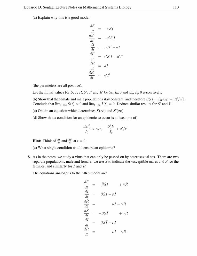
Eduardo D. Sontag, Lecture Notes on Mathematical Systems Biology 110
(a) Explain why this is a good model:
dS
dt= −rSI ′
dS ′
dt= −r′S ′I
dI
dt= rSI ′ − aI
dI ′
dt= r′S ′I − a′I ′
dR
dt= aI
dR′
dt= a′I ′
(the parameters are all positive).
Let the initial values for S, I , R, S ′, I ′ and R′ be S0, I0, 0 and S ′0, I ′0, 0 respectively.
(b) Show that the female and male populations stay constant, and therefore S(t) = S0 exp[−rR′/a′].Conclude that limt→∞ S(t) > 0 and limt→∞ I(t) = 0. Deduce similar results for S ′ and I ′.
(c) Obtain an equation which determines S(∞) and S ′(∞).
(d) Show that a condition for an epidemic to occur is at least one of:
S0I′0
I0
> a/r,S ′0I0
I ′0> a′/r′.
Hint: Think of dIdt
and dI′
dtat t = 0.
(e) What single condition would ensure an epidemic?
8. As in the notes, we study a virus that can only be passed on by heterosexual sex. There are twoseparate populations, male and female: we use S to indicate the susceptible males and S for thefemales, and similarly for I and R.
The equations analogous to the SIRS model are:
dS
dt= −βSI + γR
dI
dt= βSI − νI
dR
dt= νI − γR
dS
dt= −βSI + γR
dI
dt= βSI − νI
dR
dt= νI − γR .
Eduardo D. Sontag, Lecture Notes on Mathematical Systems Biology 111
This model is a little difficult to study, but in many STD’s (especially asymptomatic), there is no“removed” class, but instead the infecteds get back into the susceptible population. This gives:
dS
dt= −βSI + νI
dI
dt= βSI − νI
dS
dt= −βSI + νI
dI
dt= βSI − νI .
Writing N = S(t) + I(t) and N = S(t) + I(t) for the total numbers of males and females, andusing these two conservation laws, we then concluded that one may just study the following setof two ODE’s:
dI
dt= β(N − I)I − νI
dI
dt= β(N − I)I − νI .
Parts (a)-(c) refer to this reduced model.
(a) Prove that there are two equilibria, the first of which is I = I = 0 and a second one, whichexists provided that:
σσ =
(Nβ
ν
)(N β
ν
)> 1
and is given by I = NN−(νν)/(ββ)
ν/β+N, I = NN−(νν)/(ββ)
ν/β+N.
(b) Prove that the first equilibrium is unstable, and the second one stable.
(c) What vaccination strategies could be used to eradicate the disease?
(d) Now consider the full model (six dimensional, with removeds). How many linearly inde-pendent conservation laws are there?
(e) Again for the full model. Reduce by conservation to a system of 5 or less equations(how many, depends on how many conservation laws you found in (d)). Pick some setof numerical parameters (any you want) such that σσ = 2. Determine, using computersimulations, what the solutions look like. (You may be able to find the steady statesalgebraically, too.)For your answer, attach some plots of solutions I(t) and I(t) as a function of time.
1.10.6 Chemical kinetics problems
1. Suppose that the enzyme E can react with the substrate A in such a way that up to two copiesof A may bind to E at the same time. We model this by the following chemical network:
A+ Ek−1−→←−k1
C1k2−→ P + E
Eduardo D. Sontag, Lecture Notes on Mathematical Systems Biology 112
A+ C1
k−3−→←−k3
C2k2−→ P + C1
where the k’s are the rate constants, P a product of the reaction, and C1 and C2 are enzyme-substrate complexes.
(a) What are the species vector S and the reaction vector R(S)?
(b) Find the stoichiometry matrix Γ and calculate its rank.
(c) Compute the product ΓR(S), and write down the differential equation model based on massaction kinetics.
(d) Find a conservation law, assuming that a(0) = a0, e(0) = e0, c1(0) = c2(0) = p(0) = 0.
(d’) Find a basis of the left nullspace of Γ and compare it with your answer of part (d).
(e) Use part (d) and write a system of equations for just a, c1 and c2.
(f) If ε = e0a0 1, τ = k1e0t, u = a
a0, νi = ci
e0for i = 1, 2, show that the reaction mechanism
reduces to the following form in terms of the new variables (provide expressions for f and g):
du
dτ= f(u, ν1, ν2)
εdνidτ
= gi(u, ν1, ν2), i = 1, 2.
2. Consider the following chemical reaction network, which involves 4 substances calledM,E,C, P :
3M + 2E1−→←−1
C1−→ 2E + P .
(a) Find the species vector S and the reaction vector R(S) (assuming mass action kinetics).
(b) Find the stoichiometry matrix Γ.
(c) Compute the product ΓR(S) and show the set of 4 differential equations for M,E,C, P .
(d) Find the rank of Γ.
(e) What is the dimension of the left nullspace of Γ?
(f) Find a basis of the left nullspace of Γ (conservation laws).
3. We discussed the chemical kinetics formulation of an example that may be represented as inFigure 1.1(a).
Many cell signaling processes involve double instead of single transformations such as additionof phosphate groups. A model for a double-phosphorylation as in Figure 1.1(b) corresponds toreactions as follows (we use double arrows for simplicity, to indicate reversible reactions):
E + S0 ↔ ES0 → E + S1 ↔ ES1 → E + S2
F + S2 ↔ FS2 → F + S1 ↔ FS1 → F + S0(1.19)
where “ES0” represents the complex consisting of E bound to S0 and so forth.
(a) Find the stoichiometry matrix and write a corresponding system of ODE’s.
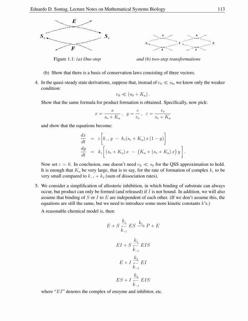
Eduardo D. Sontag, Lecture Notes on Mathematical Systems Biology 113
Figure 1.1: (a) One-step and (b) two-step transformations
(b) Show that there is a basis of conservation laws consisting of three vectors.
4. In the quasi-steady state derivations, suppose that, instead of e0 s0, we know only the weakercondition:
e0 (s0 +Km) .
Show that the same formula for product formation is obtained. Specifically, now pick:
x =s
s0 +Km
, y =c
e0, ε =
e0s0 +Km
and show that the equations become:
dx
dt= ε
[k−1 y − k1(s0 +Km)x (1− y)
]dy
dt= k1
[(s0 +Km)x −
(Km + (s0 +Km)x
)y
].
Now set ε = 0. In conclusion, one doesn’t need e0 s0 for the QSS approximation to hold.It is enough that Km be very large, that is to say, for the rate of formation of complex k1 to bevery small compared to k−1 + k2 (sum of dissociation rates).
5. We consider a simplification of allosteric inhibition, in which binding of substrate can alwaysoccur, but product can only be formed (and released) if I is not bound. In addition, we will alsoassume that binding of S or I to E are independent of each other. (If we don’t assume this, theequations are still the same, but we need to introduce some more kinetic constants k’s.)
A reasonable chemical model is, then:
E + Sk1−→←−k−1
ESk2−→ P + E
EI + Sk1−→←−k−1
EIS
E + Ik3−→←−k−3
EI
ES + Ik3−→←−k−3
EIS
where “EI” denotes the complex of enzyme and inhibitor, etc.
Eduardo D. Sontag, Lecture Notes on Mathematical Systems Biology 114
Prove that there results under quasi-steady state approximation a rate
dp
dt=
Vmax
1 + i/Ki· s
2 + as+ b
s2 + cx+ d
for some suitable numbers a = a(i), . . . and a suitably defined Ki.
6. A process in which a chemical is involved in its own production is called autocatalysis. Asimple example of autocatalysis is:
E +Xk−1−−−−k1
2X
in which a molecule of X combines with a molecule of E to produce two molecule of X .Suppose E has a constant concentration e, and that the concentration of X is x. Now answerthe following questions:
(a) Write an equation describing the system (assuming mass action kinetics).
(b) Find the steady states and their stabilities.
(c) Show that x(t)→ k1ak−1
as t→∞.
7. This problem deals with the material in the section entitled “A digression on gene expression”.
(a) Consider the full model with repression: write the stoichiometry matrix and the differentialequations, and analyze solutions.
(b) Formulate a model with activation instead of repression. (No need to analyze the model.)
8. Consider the following system:
A+Xk−1−−−−k1
2X
B +Xk2−→ C
where a molecule of X combines with a molecule of A to produce two molecules of X and amolecule of X is combines with a molecule of B to produce molecule of C. Suppose A and Bhave constant concentrations a and b and the concentration ofX is x. Now answer the followingquestions:
(a) Write an equation describing x (assuming mass action kinetics).
(b) Show that x = 0 is a steady state. Under what condition x = 0 is an unstable steady state.Is there any condition to make x = 0 a stable steady state?
(c) Show that the system exhibits a bifurcation and draw its diagram.
1.10.7 Multiple steady states, sigmoidal responses, etc. problems
1. Do this problem:
http://www.math.rutgers.edu/∼sontag/JODE/gardner cantor collins toggle.html
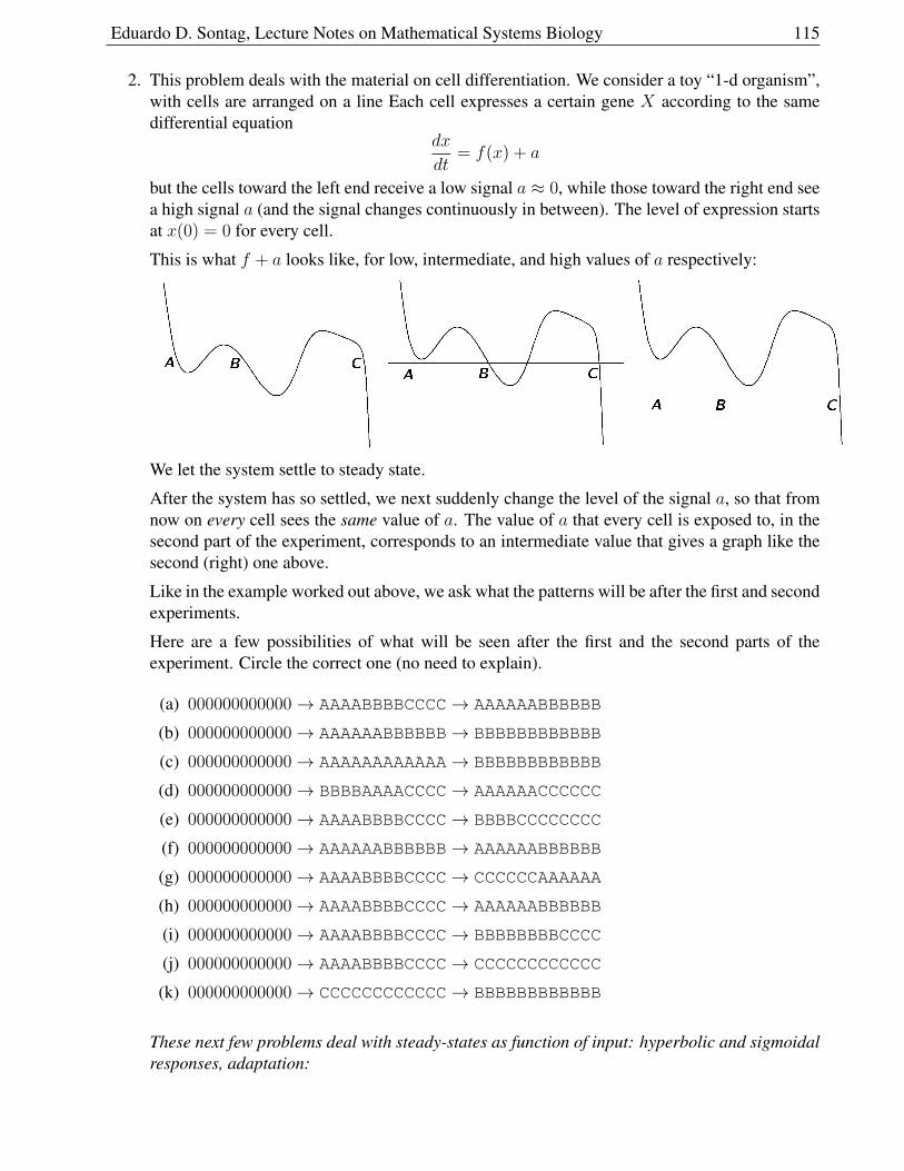
Eduardo D. Sontag, Lecture Notes on Mathematical Systems Biology 115
2. This problem deals with the material on cell differentiation. We consider a toy “1-d organism”,with cells are arranged on a line Each cell expresses a certain gene X according to the samedifferential equation
dx
dt= f(x) + a
but the cells toward the left end receive a low signal a ≈ 0, while those toward the right end seea high signal a (and the signal changes continuously in between). The level of expression startsat x(0) = 0 for every cell.
This is what f + a looks like, for low, intermediate, and high values of a respectively:
We let the system settle to steady state.
After the system has so settled, we next suddenly change the level of the signal a, so that fromnow on every cell sees the same value of a. The value of a that every cell is exposed to, in thesecond part of the experiment, corresponds to an intermediate value that gives a graph like thesecond (right) one above.
Like in the example worked out above, we ask what the patterns will be after the first and secondexperiments.
Here are a few possibilities of what will be seen after the first and the second parts of theexperiment. Circle the correct one (no need to explain).
(a) 000000000000→ AAAABBBBCCCC→ AAAAAABBBBBB
(b) 000000000000→ AAAAAABBBBBB→ BBBBBBBBBBBB
(c) 000000000000→ AAAAAAAAAAAA→ BBBBBBBBBBBB
(d) 000000000000→ BBBBAAAACCCC→ AAAAAACCCCCC
(e) 000000000000→ AAAABBBBCCCC→ BBBBCCCCCCCC
(f) 000000000000→ AAAAAABBBBBB→ AAAAAABBBBBB
(g) 000000000000→ AAAABBBBCCCC→ CCCCCCAAAAAA
(h) 000000000000→ AAAABBBBCCCC→ AAAAAABBBBBB
(i) 000000000000→ AAAABBBBCCCC→ BBBBBBBBCCCC
(j) 000000000000→ AAAABBBBCCCC→ CCCCCCCCCCCC
(k) 000000000000→ CCCCCCCCCCCC→ BBBBBBBBBBBB
These next few problems deal with steady-states as function of input: hyperbolic and sigmoidalresponses, adaptation:
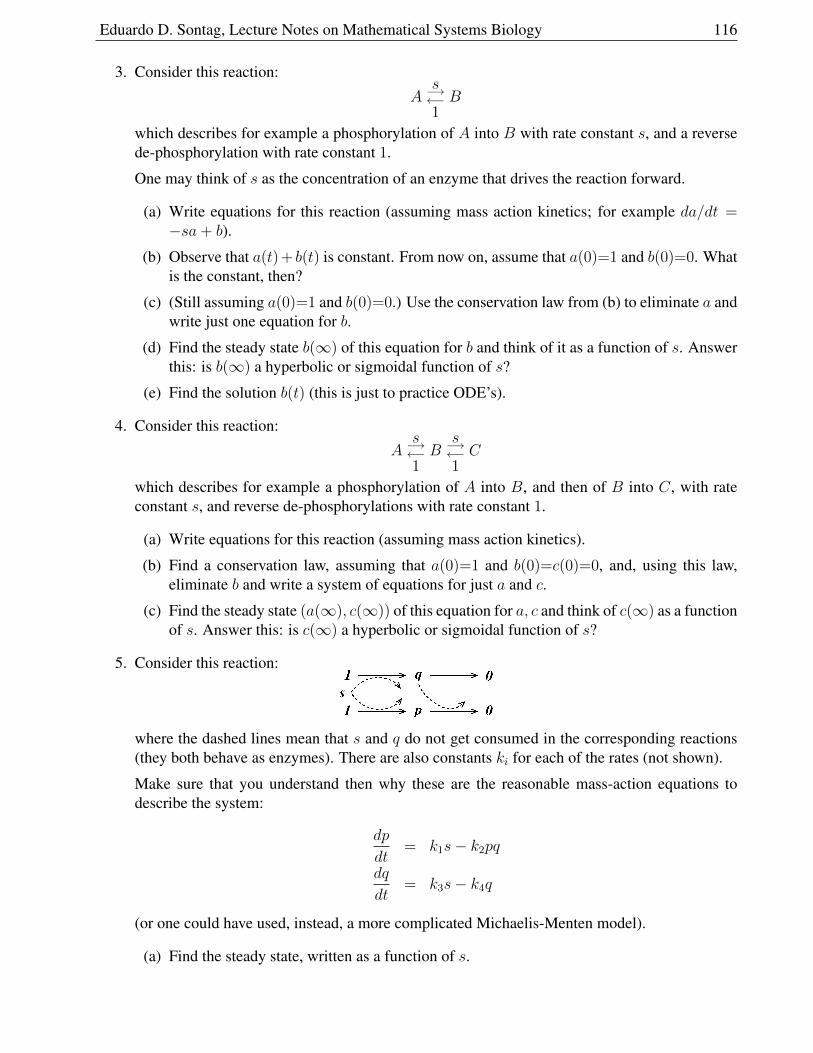
Eduardo D. Sontag, Lecture Notes on Mathematical Systems Biology 116
3. Consider this reaction:
As−→←−1B
which describes for example a phosphorylation of A into B with rate constant s, and a reversede-phosphorylation with rate constant 1.
One may think of s as the concentration of an enzyme that drives the reaction forward.
(a) Write equations for this reaction (assuming mass action kinetics; for example da/dt =−sa+ b).
(b) Observe that a(t) + b(t) is constant. From now on, assume that a(0)=1 and b(0)=0. Whatis the constant, then?
(c) (Still assuming a(0)=1 and b(0)=0.) Use the conservation law from (b) to eliminate a andwrite just one equation for b.
(d) Find the steady state b(∞) of this equation for b and think of it as a function of s. Answerthis: is b(∞) a hyperbolic or sigmoidal function of s?
(e) Find the solution b(t) (this is just to practice ODE’s).
4. Consider this reaction:
As−→←−1B
s−→←−1C
which describes for example a phosphorylation of A into B, and then of B into C, with rateconstant s, and reverse de-phosphorylations with rate constant 1.
(a) Write equations for this reaction (assuming mass action kinetics).
(b) Find a conservation law, assuming that a(0)=1 and b(0)=c(0)=0, and, using this law,eliminate b and write a system of equations for just a and c.
(c) Find the steady state (a(∞), c(∞)) of this equation for a, c and think of c(∞) as a functionof s. Answer this: is c(∞) a hyperbolic or sigmoidal function of s?
5. Consider this reaction:
where the dashed lines mean that s and q do not get consumed in the corresponding reactions(they both behave as enzymes). There are also constants ki for each of the rates (not shown).
Make sure that you understand then why these are the reasonable mass-action equations todescribe the system:
dp
dt= k1s− k2pq
dq
dt= k3s− k4q
(or one could have used, instead, a more complicated Michaelis-Menten model).
(a) Find the steady state, written as a function of s.
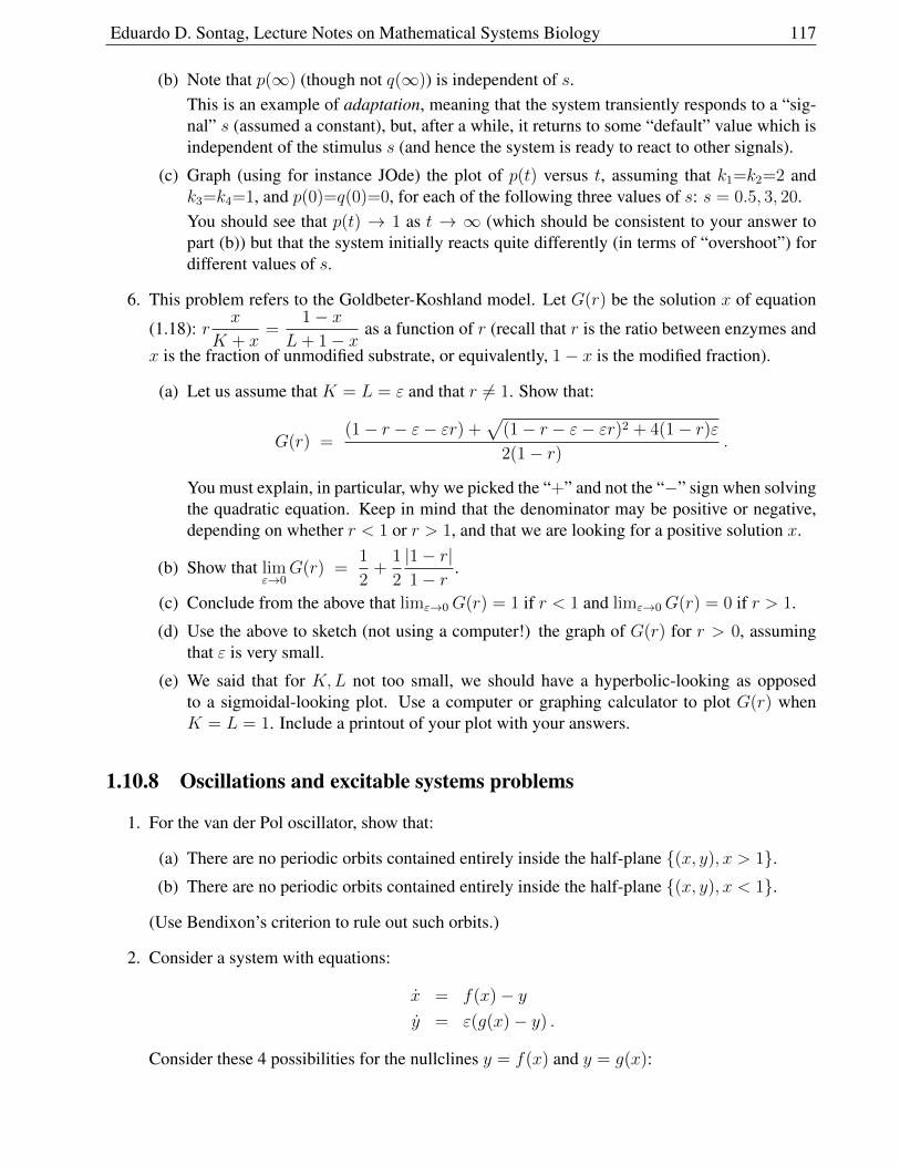
Eduardo D. Sontag, Lecture Notes on Mathematical Systems Biology 117
(b) Note that p(∞) (though not q(∞)) is independent of s.This is an example of adaptation, meaning that the system transiently responds to a “sig-nal” s (assumed a constant), but, after a while, it returns to some “default” value which isindependent of the stimulus s (and hence the system is ready to react to other signals).
(c) Graph (using for instance JOde) the plot of p(t) versus t, assuming that k1=k2=2 andk3=k4=1, and p(0)=q(0)=0, for each of the following three values of s: s = 0.5, 3, 20.You should see that p(t) → 1 as t → ∞ (which should be consistent to your answer topart (b)) but that the system initially reacts quite differently (in terms of “overshoot”) fordifferent values of s.
6. This problem refers to the Goldbeter-Koshland model. Let G(r) be the solution x of equation
(1.18): rx
K + x=
1− xL+ 1− x
as a function of r (recall that r is the ratio between enzymes and
x is the fraction of unmodified substrate, or equivalently, 1− x is the modified fraction).
(a) Let us assume that K = L = ε and that r 6= 1. Show that:
G(r) =(1− r − ε− εr) +
√(1− r − ε− εr)2 + 4(1− r)ε2(1− r)
.
You must explain, in particular, why we picked the “+” and not the “−” sign when solvingthe quadratic equation. Keep in mind that the denominator may be positive or negative,depending on whether r < 1 or r > 1, and that we are looking for a positive solution x.
(b) Show that limε→0
G(r) =1
2+
1
2
|1− r|1− r
.
(c) Conclude from the above that limε→0G(r) = 1 if r < 1 and limε→0G(r) = 0 if r > 1.
(d) Use the above to sketch (not using a computer!) the graph of G(r) for r > 0, assumingthat ε is very small.
(e) We said that for K,L not too small, we should have a hyperbolic-looking as opposedto a sigmoidal-looking plot. Use a computer or graphing calculator to plot G(r) whenK = L = 1. Include a printout of your plot with your answers.
1.10.8 Oscillations and excitable systems problems
1. For the van der Pol oscillator, show that:
(a) There are no periodic orbits contained entirely inside the half-plane (x, y), x > 1.(b) There are no periodic orbits contained entirely inside the half-plane (x, y), x < 1.
(Use Bendixon’s criterion to rule out such orbits.)
2. Consider a system with equations:
x = f(x)− yy = ε(g(x)− y) .
Consider these 4 possibilities for the nullclines y = f(x) and y = g(x):
Eduardo D. Sontag, Lecture Notes on Mathematical Systems Biology 118
(a) What can you say about stability of the steady states?
(b) Sketch directions of movement in each; use large or small arrows and use this info tosketch what trajectories should look like.
(c) Sketch what solutions x(t), y(t) look like, for each of the examples.
3. Consider the system
x1 = µx1 − ωx2 − x1(x21 + x2
2)
x2 = ωx1 + µx2 − x2(x21 + x2
2)
which we analyzed in polar coordinates. Now represent the pair (x1, x2) by the complex numberz = x1 + ix2. Show that the equation becomes, for z = z(t):
z = (µ+ ωi)z − |z|2 z .
(Hint: use that z = x1 + ix2.)
4. Check for which of the following vector fields
F (x, y) =
(f(x, y)g(x, y)
)is the unit square [0, 1] × [0, 1] a trapping region (so that one may attempt to apply Poincare-Bendixson).
(a) f(x, y) = y − x, g(x, y) = x− y(b) f(x, y) = y(x− 1), g(x, y) = −x(c) f(x, y) = x(y − 1), g(x, y) = −y(d) f(x, y) = cos π(x+ y/8), g(x, y) = x2 − y2
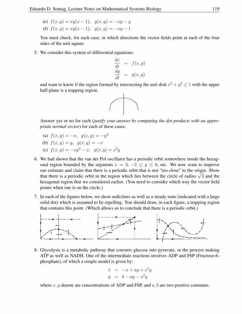
Eduardo D. Sontag, Lecture Notes on Mathematical Systems Biology 119
(e) f(x, y) = xy(x− 1), g(x, y) = −xy − y(f) f(x, y) = xy(x− 1), g(x, y) = −xy − 1
You must check, for each case, in which directions the vector fields point at each of the foursides of the unit square.
5. We consider this system of differential equations:
dx
dt= f(x, y)
dy
dt= g(x, y)
and want to know if the region formed by intersecting the unit disk x2 + y2 ≤ 1 with the upperhalf-plane is a trapping region.
Answer yes or no for each (justify your answer by computing the dot products with an appro-priate normal vector) for each of these cases:
(a) f(x, y) = −x, g(x, y) = −y2
(b) f(x, y) = y, g(x, y) = −x(c) f(x, y) = −xy2 − x, g(x, y) = x2y
6. We had shown that the van der Pol oscillator has a periodic orbit somewhere inside the hexag-onal region bounded by the segments x = 3, −3 ≤ y ≤ 6, etc. We now want to improveour estimate and claim that there is a periodic orbit that is not “too close” to the origin. Showthat there is a periodic orbit in the region which lies between the circle of radius
√3 and the
hexagonal region that we considered earlier. (You need to consider which way the vector fieldpoints when one is on the circle.)
7. In each of the figures below, we show nullclines as well as a steady state (indicated with a largesolid dot) which is assumed to be repelling. You should draw, in each figure, a trapping regionthat contains this point. (Which allows us to conclude that there is a periodic orbit.)
8. Glycolysis is a metabolic pathway that converts glucose into pyruvate, in the process makingATP as well as NADH. One of the intermediate reactions involves ADP and F6P (Fructose-6-phosphate), of which a simple model is given by:
x = −x+ ay + x2y
y = b− ay − x2y
where x, y denote are concentrations of ADP and F6P, and a, b are two positive constants.
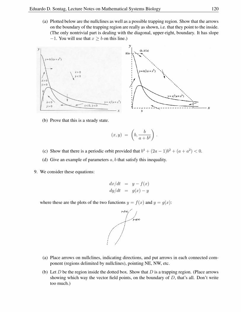
Eduardo D. Sontag, Lecture Notes on Mathematical Systems Biology 120
(a) Plotted below are the nullclines as well as a possible trapping region. Show that the arrowson the boundary of the trapping region are really as shown, i.e. that they point to the inside.(The only nontrivial part is dealing with the diagonal, upper-right, boundary. It has slope−1. You will use that x ≥ b on this line.)
(b) Prove that this is a steady state.
(x, y) =
(b,
b
a+ b2
).
(c) Show that there is a periodic orbit provided that b4 + (2a− 1)b2 + (a+ a2) < 0.
(d) Give an example of parameters a, b that satisfy this inequality.
9. We consider these equations:
dx/dt = y − f(x)
dy/dt = g(x)− y
where these are the plots of the two functions y = f(x) and y = g(x):
(a) Place arrows on nullclines, indicating directions, and put arrows in each connected com-ponent (regions delimited by nullclines), pointing NE, NW, etc.
(b) Let D be the region inside the dotted box. Show that D is a trapping region. (Place arrowsshowing which way the vector field points, on the boundary of D, that’s all. Don’t writetoo much.)
Eduardo D. Sontag, Lecture Notes on Mathematical Systems Biology 121
(c) What are the signs of the trace and the determinant of the Jacobian at the equilibriumshown in the picture?
(d) Can one apply the Poincare-Bendixson Theorem to conclude that there must be a periodicorbit inside the dotted box?
(e) Can one apply the Bendixson criterion to conclude that there cannot be any periodic orbitinside the dotted box?

Eduardo D. Sontag, Lecture Notes on Mathematical Systems Biology 122
Chapter 2
Deterministic PDE Models
2.1 Introduction to PDE models
Until now, we only considered functions of time (concentrations, populations, etc).From now on, we consider functions that also depend on space.
A typical biological example of space-dependence would be the concentration of a morphogen as afunction of space as well as time.
For example, this is a color-coded picture of a Drosophila embryo that has been stained for the proteinproducts of genes giant (blue), eve (red), and Kruppel (other colors indicate areas where two or allgenes are expressed):
One may also study space-dependence of a particular protein in a single cell. For example, thispicture1 shows the gradients of G-proteins in response to chemoattractant binding to receptors in thesurface of Dictyostelium discoideum amoebas:
2.1.1 Densities
We write space variables as x=(x1, x2, x3) (or just (x, y) in dimension 2, or (x, y, z) in dimension 3).1from Jin, Tian, Zhang, Ning, Long, Yu, Parent, Carole A., Devreotes, Peter N., “Localization of the G Protein
Complex in Living Cells During Chemotaxis,” Science 287(2000): 1034-1036.
123
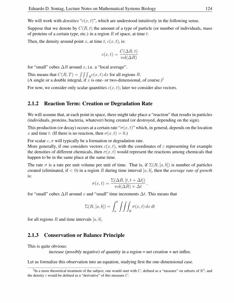
Eduardo D. Sontag, Lecture Notes on Mathematical Systems Biology 124
We will work with densities “c(x, t)”, which are understood intuitively in the following sense.
Suppose that we denote by C(R, t) the amount of a type of particle (or number of individuals, massof proteins of a certain type, etc.) in a region R of space, at time t.
Then, the density around point x, at time t, c(x, t), is:
c(x, t) =C(∆R, t)
vol(∆R)
for “small” cubes ∆R around x, i.e. a “local average”.
This means that C(R, T ) =∫ ∫ ∫
Rc(x, t) dx for all regions R.
(A single or a double integral, if x is one- or two-dimensional, of course.)2
For now, we consider only scalar quantities c(x, t); later we consider also vectors.
2.1.2 Reaction Term: Creation or Degradation Rate
We will assume that, at each point in space, there might take place a “reaction” that results in particles(individuals, proteins, bacteria, whatever) being created (or destroyed, depending on the sign).
This production (or decay) occurs at a certain rate “σ(x, t)” which, in general, depends on the locationx and time t. (If there is no reaction, then σ(x, t) = 0.)
For scalar c, σ will typically be a formation or degradation rate.More generally, if one considers vectors c(x, t), with the coordinates of c representing for examplethe densities of different chemicals, then σ(x, t) would represent the reactions among chemicals thathappen to be in the same place at the same time.
The rate σ is a rate per unit volume per unit of time. That is, if Σ(R, [a, b]) is number of particlescreated (eliminated, if < 0) in a region R during time interval [a, b], then the average rate of growthis:
σ(x, t) =Σ(∆R, [t, t+ ∆t])
vol(∆R)×∆t,
for “small” cubes ∆R around x and “small” time increments ∆t. This means that
Σ(R, [a, b]) =
∫ b
a
∫ ∫ ∫R
σ(x, t) dx dt
for all regions R and time intervals [a, b].
2.1.3 Conservation or Balance Principle
This is quite obvious:increase (possibly negative) of quantity in a region = net creation + net influx.
Let us formalize this observation into an equation, studying first the one-dimensional case.
2In a more theoretical treatment of the subject, one would start with C, defined as a “measure” on subsets of R3, andthe density c would be defined as a “derivative” of this measure C.
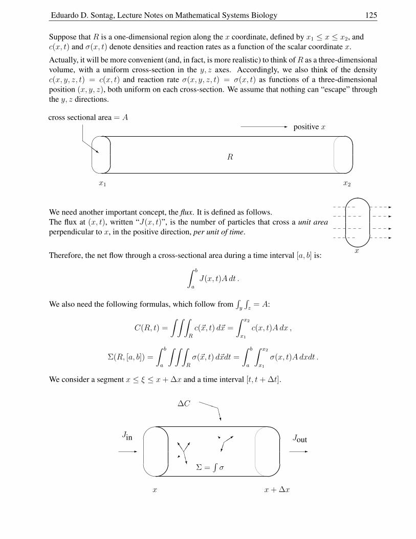
Eduardo D. Sontag, Lecture Notes on Mathematical Systems Biology 125
Suppose that R is a one-dimensional region along the x coordinate, defined by x1 ≤ x ≤ x2, andc(x, t) and σ(x, t) denote densities and reaction rates as a function of the scalar coordinate x.
Actually, it will be more convenient (and, in fact, is more realistic) to think ofR as a three-dimensionalvolume, with a uniform cross-section in the y, z axes. Accordingly, we also think of the densityc(x, y, z, t) = c(x, t) and reaction rate σ(x, y, z, t) = σ(x, t) as functions of a three-dimensionalposition (x, y, z), both uniform on each cross-section. We assume that nothing can “escape” throughthe y, z directions.
-
ZZZ~
positive xcross sectional area = A
R
x1 x2
We need another important concept, the flux. It is defined as follows.The flux at (x, t), written “J(x, t)”, is the number of particles that cross a unit areaperpendicular to x, in the positive direction, per unit of time. !
#
"-
-
-
-
xTherefore, the net flow through a cross-sectional area during a time interval [a, b] is:∫ b
a
J(x, t)Adt .
We also need the following formulas, which follow from∫y
∫z
= A:
C(R, t) =
∫ ∫ ∫R
c(~x, t) d~x =
∫ x2
x1
c(x, t)Adx ,
Σ(R, [a, b]) =
∫ b
a
∫ ∫ ∫R
σ(~x, t) d~xdt =
∫ b
a
∫ x2
x1
σ(x, t)Adxdt .
We consider a segment x ≤ ξ ≤ x+ ∆x and a time interval [t, t+ ∆t].
#
"
#
"!
!
JJ]
CCW
I3 - -
PPPCCW
x x+ ∆x
∆C
Jin Jout
Σ =∫σ
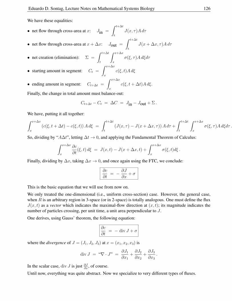
Eduardo D. Sontag, Lecture Notes on Mathematical Systems Biology 126
We have these equalities:
• net flow through cross-area at x: Jin =
∫ t+∆t
t
J(x, τ)Adτ
• net flow through cross-area at x+ ∆x: Jout =
∫ t+∆t
t
J(x+ ∆x, τ)Adτ
• net creation (elimination): Σ =
∫ t+∆t
t
∫ x+∆x
x
σ(ξ, τ)Adξdτ
• starting amount in segment: Ct =
∫ x+∆x
x
c(ξ, t)Adξ
• ending amount in segment: Ct+∆t =
∫ x+∆x
x
c(ξ, t+ ∆t)Adξ.
Finally, the change in total amount must balance-out:
Ct+∆t − Ct = ∆C = Jin − Jout + Σ .
We have, putting it all together:∫ x+∆x
x
(c(ξ, t+ ∆t)− c(ξ, t))Adξ =
∫ t+∆t
t
(J(x, τ)− J(x+ ∆x, τ))Adτ +
∫ t+∆t
t
∫ x+∆x
x
σ(ξ, τ)Adξdτ .
So, dividing by “A∆t”, letting ∆t→ 0, and applying the Fundamental Theorem of Calculus:∫ x+∆x
x
∂c
∂t(ξ, t) dξ = J(x, t)− J(x+ ∆x, t) +
∫ x+∆x
x
σ(ξ, t)dξ .
Finally, dividing by ∆x, taking ∆x→ 0, and once again using the FTC, we conclude:
∂c
∂t= − ∂J
∂x+ σ
This is the basic equation that we will use from now on.
We only treated the one-dimensional (i.e., uniform cross-section) case. However, the general case,when R is an arbitrary region in 3-space (or in 2-space) is totally analogous. One must define the fluxJ(x, t) as a vector which indicates the maximal-flow direction at (x, t); its magnitude indicates thenumber of particles crossing, per unit time, a unit area perpendicular to J .
One derives, using Gauss’ theorem, the following equation:
∂c
∂t= − div J + σ
where the divergence of J = (J1, J2, J3) at x = (x1, x2, x3) is
div J = “∇ · J” =∂J1
∂x1
+∂J2
∂x2
+∂J3
∂x3
.
In the scalar case, div J is just ∂J∂x
, of course.
Until now, everything was quite abstract. Now we specialize to very different types of fluxes.
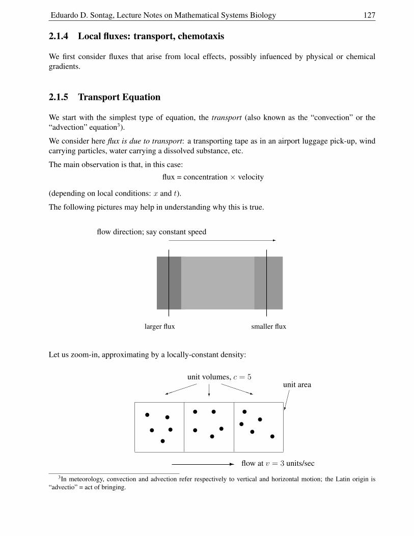
Eduardo D. Sontag, Lecture Notes on Mathematical Systems Biology 127
2.1.4 Local fluxes: transport, chemotaxis
We first consider fluxes that arise from local effects, possibly infuenced by physical or chemicalgradients.
2.1.5 Transport Equation
We start with the simplest type of equation, the transport (also known as the “convection” or the“advection” equation3).
We consider here flux is due to transport: a transporting tape as in an airport luggage pick-up, windcarrying particles, water carrying a dissolved substance, etc.
The main observation is that, in this case:
flux = concentration × velocity
(depending on local conditions: x and t).
The following pictures may help in understanding why this is true.
-
smaller flux
flow direction; say constant speed
larger flux
Let us zoom-in, approximating by a locally-constant density:
uu uuuuu uuuuu u u u
) ?
PPPPPq
-
unit volumes, c = 5unit area
flow at v = 3 units/sec
3In meteorology, convection and advection refer respectively to vertical and horizontal motion; the Latin origin is“advectio” = act of bringing.
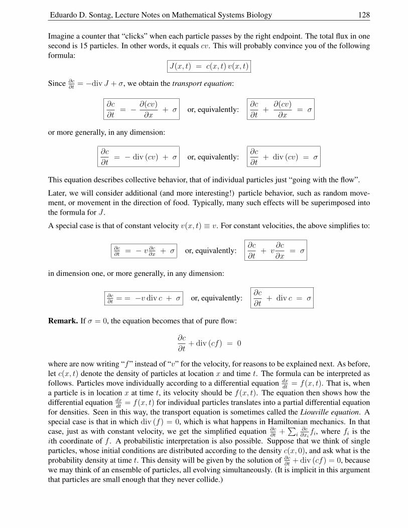
Eduardo D. Sontag, Lecture Notes on Mathematical Systems Biology 128
Imagine a counter that “clicks” when each particle passes by the right endpoint. The total flux in onesecond is 15 particles. In other words, it equals cv. This will probably convince you of the followingformula:
J(x, t) = c(x, t) v(x, t)
Since ∂c∂t
= −div J + σ, we obtain the transport equation:
∂c
∂t= − ∂(cv)
∂x+ σ or, equivalently:
∂c
∂t+
∂(cv)
∂x= σ
or more generally, in any dimension:
∂c
∂t= − div (cv) + σ or, equivalently:
∂c
∂t+ div (cv) = σ
This equation describes collective behavior, that of individual particles just “going with the flow”.
Later, we will consider additional (and more interesting!) particle behavior, such as random move-ment, or movement in the direction of food. Typically, many such effects will be superimposed intothe formula for J .
A special case is that of constant velocity v(x, t) ≡ v. For constant velocities, the above simplifies to:
∂c∂t
= − v ∂c∂x
+ σ or, equivalently:∂c
∂t+ v
∂c
∂x= σ
in dimension one, or more generally, in any dimension:
∂c∂t
= = −v div c + σ or, equivalently:∂c
∂t+ div c = σ
Remark. If σ = 0, the equation becomes that of pure flow:
∂c
∂t+ div (cf) = 0
where are now writing “f” instead of “v” for the velocity, for reasons to be explained next. As before,let c(x, t) denote the density of particles at location x and time t. The formula can be interpreted asfollows. Particles move individually according to a differential equation dx
dt= f(x, t). That is, when
a particle is in location x at time t, its velocity should be f(x, t). The equation then shows how thedifferential equation dx
dt= f(x, t) for individual particles translates into a partial differential equation
for densities. Seen in this way, the transport equation is sometimes called the Liouville equation. Aspecial case is that in which div (f) = 0, which is what happens in Hamiltonian mechanics. In thatcase, just as with constant velocity, we get the simplified equation ∂c
∂t+∑
i∂c∂xifi, where fi is the
ith coordinate of f . A probabilistic interpretation is also possible. Suppose that we think of singleparticles, whose initial conditions are distributed according to the density c(x, 0), and ask what is theprobability density at time t. This density will be given by the solution of ∂c
∂t+ div (cf) = 0, because
we may think of an ensemble of particles, all evolving simultaneously. (It is implicit in this argumentthat particles are small enough that they never collide.)
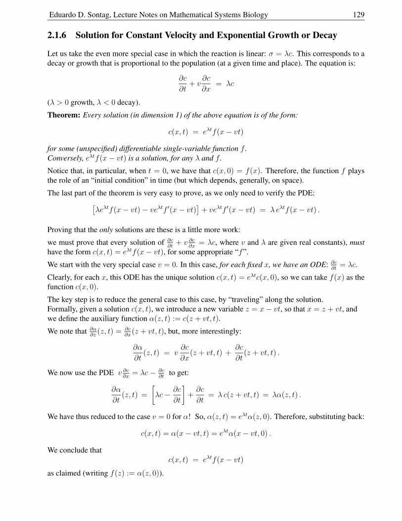
Eduardo D. Sontag, Lecture Notes on Mathematical Systems Biology 129
2.1.6 Solution for Constant Velocity and Exponential Growth or Decay
Let us take the even more special case in which the reaction is linear: σ = λc. This corresponds to adecay or growth that is proportional to the population (at a given time and place). The equation is:
∂c
∂t+ v
∂c
∂x= λc
(λ > 0 growth, λ < 0 decay).
Theorem: Every solution (in dimension 1) of the above equation is of the form:
c(x, t) = eλtf(x− vt)
for some (unspecified) differentiable single-variable function f .Conversely, eλtf(x− vt) is a solution, for any λ and f .
Notice that, in particular, when t = 0, we have that c(x, 0) = f(x). Therefore, the function f playsthe role of an “initial condition” in time (but which depends, generally, on space).
The last part of the theorem is very easy to prove, as we only need to verify the PDE:[λeλtf(x− vt)− veλtf ′(x− vt)
]+ veλtf ′(x− vt) = λ eλtf(x− vt) .
Proving that the only solutions are these is a little more work:
we must prove that every solution of ∂c∂t
+ v ∂c∂x
= λc, where v and λ are given real constants), musthave the form c(x, t) = eλtf(x− vt), for some appropriate “f”.
We start with the very special case v = 0. In this case, for each fixed x, we have an ODE: ∂c∂t
= λc.
Clearly, for each x, this ODE has the unique solution c(x, t) = eλtc(x, 0), so we can take f(x) as thefunction c(x, 0).
The key step is to reduce the general case to this case, by “traveling” along the solution.Formally, given a solution c(x, t), we introduce a new variable z = x− vt, so that x = z + vt, andwe define the auxiliary function α(z, t) := c(z + vt, t).
We note that ∂α∂z
(z, t) = ∂c∂x
(z + vt, t), but, more interestingly:
∂α
∂t(z, t) = v
∂c
∂x(z + vt, t) +
∂c
∂t(z + vt, t) .
We now use the PDE v ∂c∂x
= λc− ∂c∂t
to get:
∂α
∂t(z, t) =
[λc− ∂c
∂t
]+∂c
∂t= λ c(z + vt, t) = λα(z, t) .
We have thus reduced to the case v = 0 for α! So, α(z, t) = eλtα(z, 0). Therefore, substituting back:
c(x, t) = α(x− vt, t) = eλtα(x− vt, 0) .
We conclude thatc(x, t) = eλtf(x− vt)
as claimed (writing f(z) := α(z, 0)).
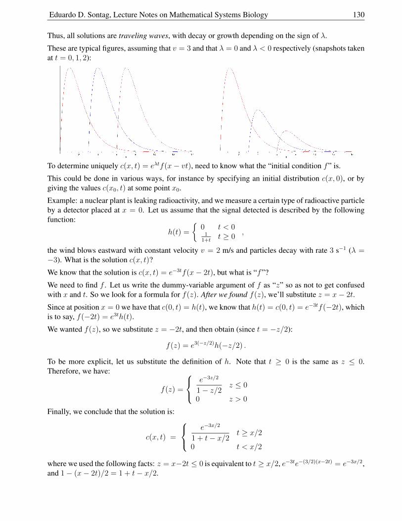
Eduardo D. Sontag, Lecture Notes on Mathematical Systems Biology 130
Thus, all solutions are traveling waves, with decay or growth depending on the sign of λ.
These are typical figures, assuming that v = 3 and that λ = 0 and λ < 0 respectively (snapshots takenat t = 0, 1, 2):
To determine uniquely c(x, t) = eλtf(x− vt), need to know what the “initial condition f” is.
This could be done in various ways, for instance by specifying an initial distribution c(x, 0), or bygiving the values c(x0, t) at some point x0.
Example: a nuclear plant is leaking radioactivity, and we measure a certain type of radioactive particleby a detector placed at x = 0. Let us assume that the signal detected is described by the followingfunction:
h(t) =
0 t < 0
11+t
t ≥ 0,
the wind blows eastward with constant velocity v = 2 m/s and particles decay with rate 3 s−1 (λ =−3). What is the solution c(x, t)?
We know that the solution is c(x, t) = e−3tf(x− 2t), but what is “f”?
We need to find f . Let us write the dummy-variable argument of f as “z” so as not to get confusedwith x and t. So we look for a formula for f(z). After we found f(z), we’ll substitute z = x− 2t.
Since at position x = 0 we have that c(0, t) = h(t), we know that h(t) = c(0, t) = e−3tf(−2t), whichis to say, f(−2t) = e3th(t).
We wanted f(z), so we substitute z = −2t, and then obtain (since t = −z/2):
f(z) = e3(−z/2)h(−z/2) .
To be more explicit, let us substitute the definition of h. Note that t ≥ 0 is the same as z ≤ 0.Therefore, we have:
f(z) =
e−3z/2
1− z/2z ≤ 0
0 z > 0
Finally, we conclude that the solution is:
c(x, t) =
e−3x/2
1 + t− x/2t ≥ x/2
0 t < x/2
where we used the following facts: z = x−2t ≤ 0 is equivalent to t ≥ x/2, e−3te−(3/2)(x−2t) = e−3x/2,and 1− (x− 2t)/2 = 1 + t− x/2.
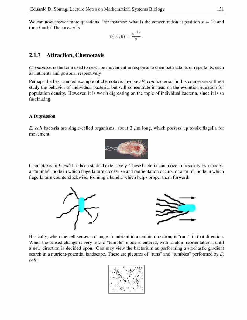
Eduardo D. Sontag, Lecture Notes on Mathematical Systems Biology 131
We can now answer more questions. For instance: what is the concentration at position x = 10 andtime t = 6? The answer is
c(10, 6) =e−15
2.
2.1.7 Attraction, Chemotaxis
Chemotaxis is the term used to describe movement in response to chemoattractants or repellants, suchas nutrients and poisons, respectively.
Perhaps the best-studied example of chemotaxis involves E. coli bacteria. In this course we will notstudy the behavior of individual bacteria, but will concentrate instead on the evolution equation forpopulation density. However, it is worth digressing on the topic of individual bacteria, since it is sofascinating.
A Digression
E. coli bacteria are single-celled organisms, about 2 µm long, which possess up to six flagella formovement.
Chemotaxis in E. coli has been studied extensively. These bacteria can move in basically two modes:a “tumble” mode in which flagella turn clockwise and reorientation occurs, or a “run” mode in whichflagella turn counterclockwise, forming a bundle which helps propel them forward.
Basically, when the cell senses a change in nutrient in a certain direction, it “runs” in that direction.When the sensed change is very low, a “tumble” mode is entered, with random reorientations, untila new direction is decided upon. One may view the bacterium as performing a stochastic gradientsearch in a nutrient-potential landscape. These are pictures of “runs” and “tumbles” performed by E.coli:
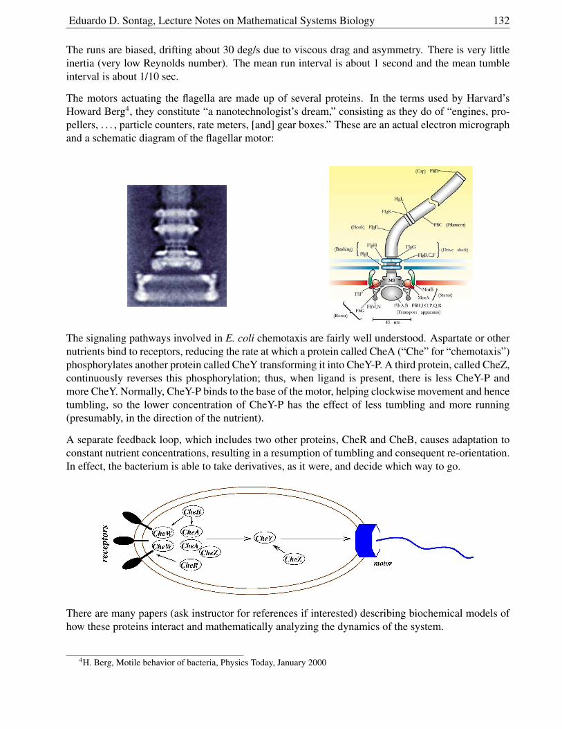
Eduardo D. Sontag, Lecture Notes on Mathematical Systems Biology 132
The runs are biased, drifting about 30 deg/s due to viscous drag and asymmetry. There is very littleinertia (very low Reynolds number). The mean run interval is about 1 second and the mean tumbleinterval is about 1/10 sec.
The motors actuating the flagella are made up of several proteins. In the terms used by Harvard’sHoward Berg4, they constitute “a nanotechnologist’s dream,” consisting as they do of “engines, pro-pellers, . . . , particle counters, rate meters, [and] gear boxes.” These are an actual electron micrographand a schematic diagram of the flagellar motor:
The signaling pathways involved in E. coli chemotaxis are fairly well understood. Aspartate or othernutrients bind to receptors, reducing the rate at which a protein called CheA (“Che” for “chemotaxis”)phosphorylates another protein called CheY transforming it into CheY-P. A third protein, called CheZ,continuously reverses this phosphorylation; thus, when ligand is present, there is less CheY-P andmore CheY. Normally, CheY-P binds to the base of the motor, helping clockwise movement and hencetumbling, so the lower concentration of CheY-P has the effect of less tumbling and more running(presumably, in the direction of the nutrient).
A separate feedback loop, which includes two other proteins, CheR and CheB, causes adaptation toconstant nutrient concentrations, resulting in a resumption of tumbling and consequent re-orientation.In effect, the bacterium is able to take derivatives, as it were, and decide which way to go.
There are many papers (ask instructor for references if interested) describing biochemical models ofhow these proteins interact and mathematically analyzing the dynamics of the system.
4H. Berg, Motile behavior of bacteria, Physics Today, January 2000
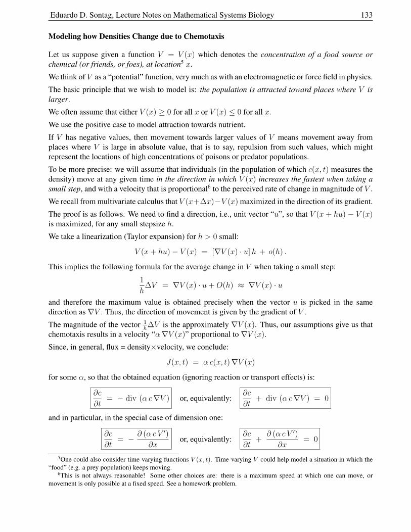
Eduardo D. Sontag, Lecture Notes on Mathematical Systems Biology 133
Modeling how Densities Change due to Chemotaxis
Let us suppose given a function V = V (x) which denotes the concentration of a food source orchemical (or friends, or foes), at location5 x.
We think of V as a “potential” function, very much as with an electromagnetic or force field in physics.
The basic principle that we wish to model is: the population is attracted toward places where V islarger.
We often assume that either V (x) ≥ 0 for all x or V (x) ≤ 0 for all x.
We use the positive case to model attraction towards nutrient.
If V has negative values, then movement towards larger values of V means movement away fromplaces where V is large in absolute value, that is to say, repulsion from such values, which mightrepresent the locations of high concentrations of poisons or predator populations.
To be more precise: we will assume that individuals (in the population of which c(x, t) measures thedensity) move at any given time in the direction in which V (x) increases the fastest when taking asmall step, and with a velocity that is proportional6 to the perceived rate of change in magnitude of V .
We recall from multivariate calculus that V (x+∆x)−V (x) maximized in the direction of its gradient.
The proof is as follows. We need to find a direction, i.e., unit vector “u”, so that V (x + hu) − V (x)is maximized, for any small stepsize h.
We take a linearization (Taylor expansion) for h > 0 small:
V (x+ hu)− V (x) = [∇V (x) · u]h + o(h) .
This implies the following formula for the average change in V when taking a small step:
1
h∆V = ∇V (x) · u+O(h) ≈ ∇V (x) · u
and therefore the maximum value is obtained precisely when the vector u is picked in the samedirection as∇V . Thus, the direction of movement is given by the gradient of V .
The magnitude of the vector 1h∆V is the approximately ∇V (x). Thus, our assumptions give us that
chemotaxis results in a velocity “α∇V (x)” proportional to∇V (x).
Since, in general, flux = density×velocity, we conclude:
J(x, t) = α c(x, t)∇V (x)
for some α, so that the obtained equation (ignoring reaction or transport effects) is:
∂c
∂t= − div (α c∇V ) or, equivalently:
∂c
∂t+ div (α c∇V ) = 0
and in particular, in the special case of dimension one:
∂c
∂t= − ∂ (α c V ′)
∂xor, equivalently:
∂c
∂t+
∂ (α c V ′)
∂x= 0
5One could also consider time-varying functions V (x, t). Time-varying V could help model a situation in which the“food” (e.g. a prey population) keeps moving.
6This is not always reasonable! Some other choices are: there is a maximum speed at which one can move, ormovement is only possible at a fixed speed. See a homework problem.
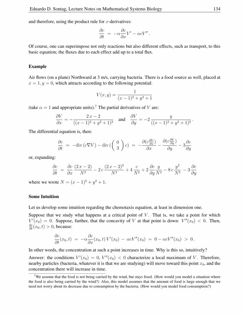
Eduardo D. Sontag, Lecture Notes on Mathematical Systems Biology 134
and therefore, using the product rule for x-derivatives:
∂c
∂t= −α ∂c
∂xV ′ − αcV ′′ .
Of course, one can superimpose not only reactions but also different effects, such as transport, to thisbasic equation; the fluxes due to each effect add up to a total flux.
Example
Air flows (on a plane) Northward at 3 m/s, carrying bacteria. There is a food source as well, placed atx = 1, y = 0, which attracts according to the following potential:
V (x, y) =1
(x− 1)2 + y2 + 1
(take α = 1 and appropriate units).7 The partial derivatives of V are:
∂V
∂x= − 2x− 2
((x− 1)2 + y2 + 1)2and
∂V
∂y= −2
y
((x− 1)2 + y2 + 1)2.
The differential equation is, then:
∂c
∂t= −div (c∇V )− div (
(03
)c) = −
∂(c∂V∂x
)
∂x−∂(c∂V
∂y)
∂y− 3
∂c
∂y
or, expanding:
∂c
∂t=
∂c
∂x
(2x− 2)
N2− 2 c
(2x− 2)2
N3+ 4
c
N2+ 2
∂c
∂y
y
N2− 8 c
y2
N3− 3
∂c
∂y
where we wrote N = (x− 1)2 + y2 + 1.
Some Intuition
Let us develop some intuition regarding the chemotaxis equation, at least in dimension one.
Suppose that we study what happens at a critical point of V . That is, we take a point for whichV ′(x0) = 0. Suppose, further, that the concavity of V at that point is down: V ′′(x0) < 0. Then,∂c∂t
(x0, t) > 0, because:
∂c
∂t(x0, t) = −α ∂c
∂x(x0, t)V
′(x0) − αcV ′′(x0) = 0− αcV ′′(x0) > 0 .
In other words, the concentration at such a point increases in time. Why is this so, intuitively?
Answer: the conditions V ′(x0) = 0, V ′′(x0) < 0 characterize a local maximum of V . Therefore,nearby particles (bacteria, whatever it is that we are studying) will move toward this point x0, and theconcentration there will increase in time.
7We assume that the food is not being carried by the wind, but stays fixed. (How would you model a situation wherethe food is also being carried by the wind?) Also, this model assumes that the amount of food is large enough that weneed not worry about its decrease due to consumption by the bacteria. (How would you model food consumption?)
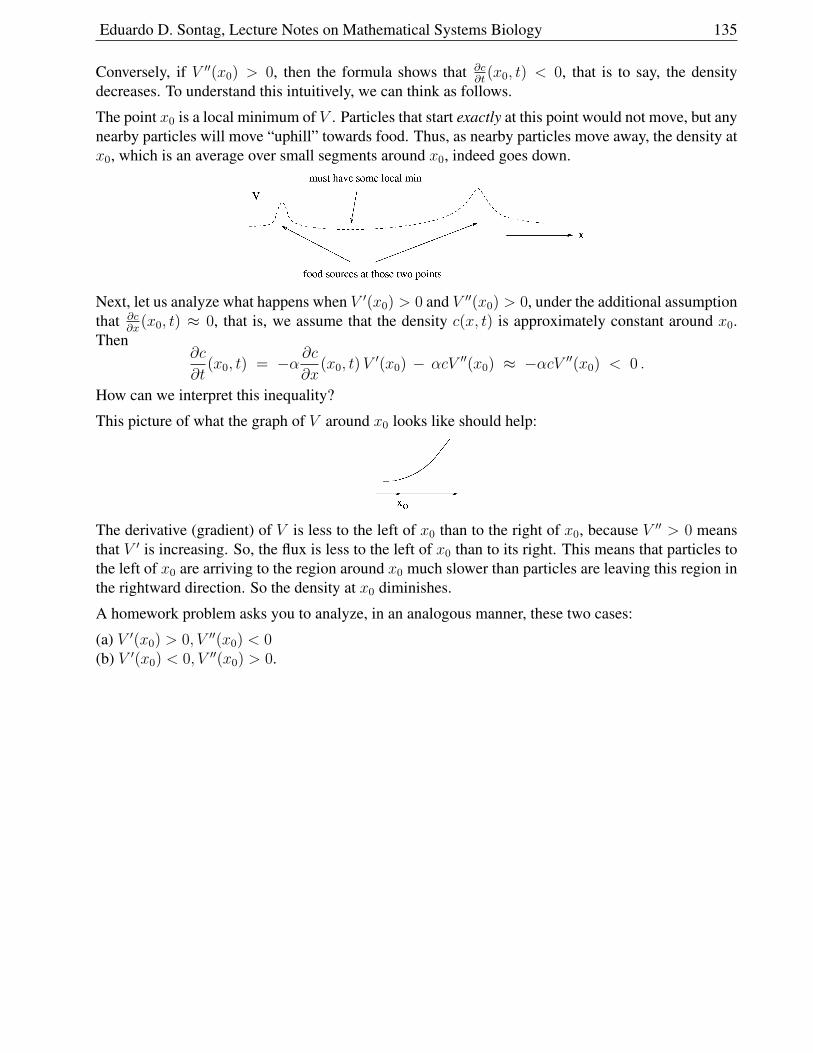
Eduardo D. Sontag, Lecture Notes on Mathematical Systems Biology 135
Conversely, if V ′′(x0) > 0, then the formula shows that ∂c∂t
(x0, t) < 0, that is to say, the densitydecreases. To understand this intuitively, we can think as follows.
The point x0 is a local minimum of V . Particles that start exactly at this point would not move, but anynearby particles will move “uphill” towards food. Thus, as nearby particles move away, the density atx0, which is an average over small segments around x0, indeed goes down.
Next, let us analyze what happens when V ′(x0) > 0 and V ′′(x0) > 0, under the additional assumptionthat ∂c
∂x(x0, t) ≈ 0, that is, we assume that the density c(x, t) is approximately constant around x0.
Then∂c
∂t(x0, t) = −α ∂c
∂x(x0, t)V
′(x0) − αcV ′′(x0) ≈ −αcV ′′(x0) < 0 .
How can we interpret this inequality?
This picture of what the graph of V around x0 looks like should help:
The derivative (gradient) of V is less to the left of x0 than to the right of x0, because V ′′ > 0 meansthat V ′ is increasing. So, the flux is less to the left of x0 than to its right. This means that particles tothe left of x0 are arriving to the region around x0 much slower than particles are leaving this region inthe rightward direction. So the density at x0 diminishes.
A homework problem asks you to analyze, in an analogous manner, these two cases:
(a) V ′(x0) > 0, V ′′(x0) < 0(b) V ′(x0) < 0, V ′′(x0) > 0.
Eduardo D. Sontag, Lecture Notes on Mathematical Systems Biology 136
2.2 Non-local fluxes: diffusion
Diffusion is one of the fundamental processes by which “particles” (atoms, molecules, even biggerobjects) move.
Fick’s Law, proposed in 1855, and based upon experimental observations, postulated that diffusion isdue to movement from higher to lower concentration regions. Mathematically:
J(x, t) ∝ −∇c(x, t)
(we use “∝” for “proportional”).
This formula applies to movement of particles in a solution, where the proportionality constant willdepend on the sizes of the molecules involved (solvent and solute) as well as temperature. It alsoapplies in many other situations, such as for instance diffusion across membranes, in which case theconstant depends on permeability and thickness as well.
The main physical explanation of diffusion is probabilistic, based on the thermal motion of individ-ual particles due to the environment (e.g., molecules of solvent) constantly “kicking” the particles.“Brownian motion”, named after the botanist Robert Brown, refers to such random thermal motion.
One often finds the claim that Brown in his 1828 paper observed that pollen grains suspendedin water move in a rapid but very irregular fashion.
However, in Nature’s 10 March 2005 issue (see also errata in the 24 March issue), DavidWilkinson states: “. . . several authors repeat the mistaken idea that the botanist Robert Brownobserved the motion that now carries his name while watching the irregular motion of pollengrains in water. The microscopic particles involved in the characteristic jiggling dance Browndescribed were much smaller particles. I have regularly studied pollen grains in water suspensionunder a microscope without ever observing Brownian motion.
From the title of Brown’s 1828 paper “A Brief Account of Microscopical Observations ... onthe Particles contained in the Pollen of Plants...”, it is clear that he knew he was looking at smallerparticles (which he estimated at about 1/500 of an inch in diameter) than the pollen grains.
Having observed ’vivid motion’ in these particles, he next wondered if they were alive, as theyhad come from a living plant. So he looked at particles from pollen collected from old herbariumsheets (and so presumably dead) but also found the motion. He then looked at powdered fossilplant material and finally inanimate material, which all showed similar motion.
Brown’s observations convinced him that life was not necessary for the movement of thesemicroscopic particles.”
The relation to Fick’s Law was explained mathematically in Einstein’s Ph.D. thesis (1905).8
When diffusion acts, and if there are no additional constraints, the eventual result is a homogeneousconcentration over space. However, usually there are additional boundary conditions, creation andabsorption rates, etc., which are superimposed on pure diffusion. This results in a “trade-off” betweenthe “smoothing out” effects of diffusion and other influences, and the results can be very interesting.
We should also remark that diffusion is often used to model macroscopic situations analogous tomovement of particles from high to low density regions. For example, a human population may shifttowards areas with less density of population, because there is more free land to cultivate.
8A course project asks you to run a java applet simulation of Einstein’s description of Brownian motion.
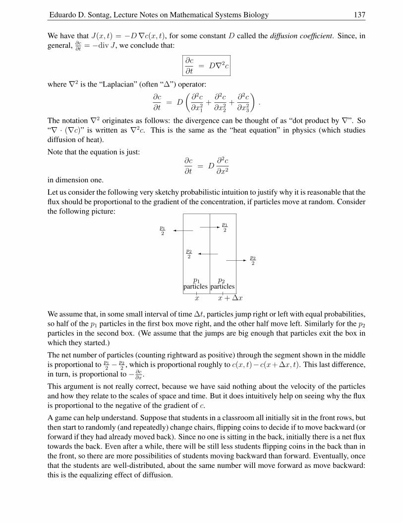
Eduardo D. Sontag, Lecture Notes on Mathematical Systems Biology 137
We have that J(x, t) = −D∇c(x, t), for some constant D called the diffusion coefficient. Since, ingeneral, ∂c
∂t= −div J , we conclude that:
∂c
∂t= D∇2c
where∇2 is the “Laplacian” (often “∆”) operator:
∂c
∂t= D
(∂2c
∂x21
+∂2c
∂x22
+∂2c
∂x23
).
The notation ∇2 originates as follows: the divergence can be thought of as “dot product by ∇”. So“∇ · (∇c)” is written as ∇2c. This is the same as the “heat equation” in physics (which studiesdiffusion of heat).
Note that the equation is just:∂c
∂t= D
∂2c
∂x2
in dimension one.
Let us consider the following very sketchy probabilistic intuition to justify why it is reasonable that theflux should be proportional to the gradient of the concentration, if particles move at random. Considerthe following picture:
-
-
p12
p12
p22 p2
2
p1particles
p2particles
x x+ ∆x
We assume that, in some small interval of time ∆t, particles jump right or left with equal probabilities,so half of the p1 particles in the first box move right, and the other half move left. Similarly for the p2
particles in the second box. (We assume that the jumps are big enough that particles exit the box inwhich they started.)
The net number of particles (counting rightward as positive) through the segment shown in the middleis proportional to p1
2− p2
2, which is proportional roughly to c(x, t)−c(x+∆x, t). This last difference,
in turn, is proportional to − ∂c∂x
.
This argument is not really correct, because we have said nothing about the velocity of the particlesand how they relate to the scales of space and time. But it does intuitively help on seeing why the fluxis proportional to the negative of the gradient of c.
A game can help understand. Suppose that students in a classroom all initially sit in the front rows, butthen start to randomly (and repeatedly) change chairs, flipping coins to decide if to move backward (orforward if they had already moved back). Since no one is sitting in the back, initially there is a net fluxtowards the back. Even after a while, there will be still less students flipping coins in the back than inthe front, so there are more possibilities of students moving backward than forward. Eventually, oncethat the students are well-distributed, about the same number will move forward as move backward:this is the equalizing effect of diffusion.
Eduardo D. Sontag, Lecture Notes on Mathematical Systems Biology 138
2.2.1 Time of Diffusion (in dimension 1)
It is often said that “diffusion results in movement proportional to√t”. The following theorem gives
one way to make that statement precise. A different interpretation is in the next section, and later, wewill discuss a probabilistic interpretation and relations to random walks as well.
Theorem. Suppose that c satisfies diffusion equation
∂c
∂t= D
∂2c
∂x2.
Assume also that the following hold:
C =
∫ +∞
−∞c(x, t) dx
is independent of t (constant population), and c is “small at infinity”:
for all t ≥ 0, limx→±∞
x2 ∂c
∂x(x, t) = 0 and lim
x→±∞xc(x, t) = 0 .
Define, for each t, the following integral which measures how the density “spreads out”:
σ2(t) =1
C
∫ +∞
−∞x2c(x, t) dx
(the second moment, which we assume is finite). Then:
σ2(t) = 2D t + σ2(0)
for all t. In particular, if the initial (at time t = 0) population is concentrated near x = 0 (a “δfunction”), then σ2(t) ≈ 2D t.
Proof:We use the diffusion PDE, and integrate by parts twice:
C
D
dσ2
dt=
1
D
∂
∂t
∫ +∞
−∞x2c dx =
1
D
∫ +∞
−∞x2∂c
∂tdx =
∫ +∞
−∞x2 ∂
2c
∂x2dx
=
[x2 ∂c
∂x
]+∞
−∞−∫ +∞
−∞2x∂c
∂xdx
= − [2xc]+∞−∞ +
∫ +∞
−∞2c dx = 2
∫ +∞
−∞c(x, t) dx = 2C
Canceling C, we obtain:dσ2
dt(t) = 2D
and hence, integrating over t, we have, as wanted:
σ2(t) = 2Dt+ σ2(0) .
If, in particular, particles start concentrated in a small interval around x = 0, we have that c(x, 0) = 0for all |x| > ε. Then, (with c = c(x, 0)):∫ +∞
−∞x2c dx =
∫ +ε
−εx2c dx ≤ ε2
∫ +ε
−εc dx = ε2C
so σ2(0) = ε2 ≈ 0.
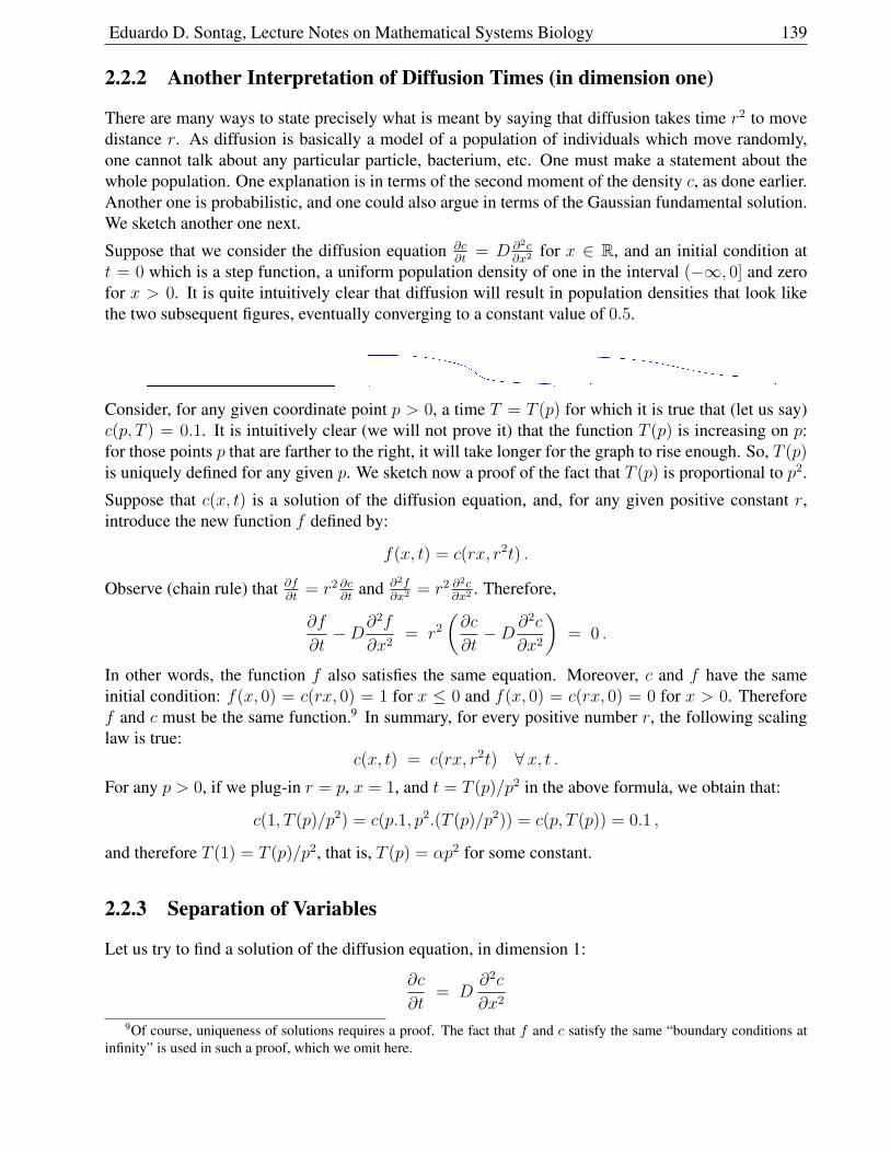
Eduardo D. Sontag, Lecture Notes on Mathematical Systems Biology 139
2.2.2 Another Interpretation of Diffusion Times (in dimension one)
There are many ways to state precisely what is meant by saying that diffusion takes time r2 to movedistance r. As diffusion is basically a model of a population of individuals which move randomly,one cannot talk about any particular particle, bacterium, etc. One must make a statement about thewhole population. One explanation is in terms of the second moment of the density c, as done earlier.Another one is probabilistic, and one could also argue in terms of the Gaussian fundamental solution.We sketch another one next.
Suppose that we consider the diffusion equation ∂c∂t
= D ∂2c∂x2
for x ∈ R, and an initial condition att = 0 which is a step function, a uniform population density of one in the interval (−∞, 0] and zerofor x > 0. It is quite intuitively clear that diffusion will result in population densities that look likethe two subsequent figures, eventually converging to a constant value of 0.5.
Consider, for any given coordinate point p > 0, a time T = T (p) for which it is true that (let us say)c(p, T ) = 0.1. It is intuitively clear (we will not prove it) that the function T (p) is increasing on p:for those points p that are farther to the right, it will take longer for the graph to rise enough. So, T (p)is uniquely defined for any given p. We sketch now a proof of the fact that T (p) is proportional to p2.
Suppose that c(x, t) is a solution of the diffusion equation, and, for any given positive constant r,introduce the new function f defined by:
f(x, t) = c(rx, r2t) .
Observe (chain rule) that ∂f∂t
= r2 ∂c∂t
and ∂2f∂x2
= r2 ∂2c∂x2
. Therefore,
∂f
∂t−D∂
2f
∂x2= r2
(∂c
∂t−D∂2c
∂x2
)= 0 .
In other words, the function f also satisfies the same equation. Moreover, c and f have the sameinitial condition: f(x, 0) = c(rx, 0) = 1 for x ≤ 0 and f(x, 0) = c(rx, 0) = 0 for x > 0. Thereforef and c must be the same function.9 In summary, for every positive number r, the following scalinglaw is true:
c(x, t) = c(rx, r2t) ∀x, t .For any p > 0, if we plug-in r = p, x = 1, and t = T (p)/p2 in the above formula, we obtain that:
c(1, T (p)/p2) = c(p.1, p2.(T (p)/p2)) = c(p, T (p)) = 0.1 ,
and therefore T (1) = T (p)/p2, that is, T (p) = αp2 for some constant.
2.2.3 Separation of Variables
Let us try to find a solution of the diffusion equation, in dimension 1:
∂c
∂t= D
∂2c
∂x2
9Of course, uniqueness of solutions requires a proof. The fact that f and c satisfy the same “boundary conditions atinfinity” is used in such a proof, which we omit here.
Eduardo D. Sontag, Lecture Notes on Mathematical Systems Biology 140
of the special form c(x, t) = X(x)T (t).
Substituting into the PDE, we conclude that X,T must satisfy:
T ′(t)X(x) = DT (t)X ′′(x)
(using primes for derivatives with respect to t and x), and this must hold for all t and x, or equivalently:
DX ′′(x)
X(x)=
T ′(t)
T (t)∀x, t .
Now define:
λ :=T ′(0)
T (0)
so:
DX ′′(x)
X(x)=
T ′(0)
T (0)= λ
for all x (since the above equality holds, in particular, at t = 0). Thus, we conclude, applying theequality yet again:
DX ′′(x)
X(x)=
T ′(t)
T (t)= λ ∀x, t
for this fixed (and so far unknown) real number λ.
In other words, each of X and T satisfy an ordinary (and linear) differential equation, but the twoequations share the same λ:
X ′′(x) = λX(x)
T ′(t) = λT (t) .
(We take D=1 for simplicity.) The second of these says that T ′ = λT , i.e.
T (t) = eλtT (0)
and the first equation has the general solution (if λ 6= 0) X(x) = aeµ1x + beµ2x, where the µi’s arethe two square roots of λ, and a, b are arbitrary constants. As you saw in your diff equs course, whenλ < 0, it is more user-friendly to write complex exponentials as trigonometric functions, which alsohas the advantage that a, b can then be taken as real numbers (especially useful since a and b areusually fit to initial conditions). In summary, for λ > 0 one has:
X(x) = aeµx + be−µx
(with µ =√λ), while for λ < 0 one has:
X(x) = a cos kx+ b sin kx
(with k =√−λ).
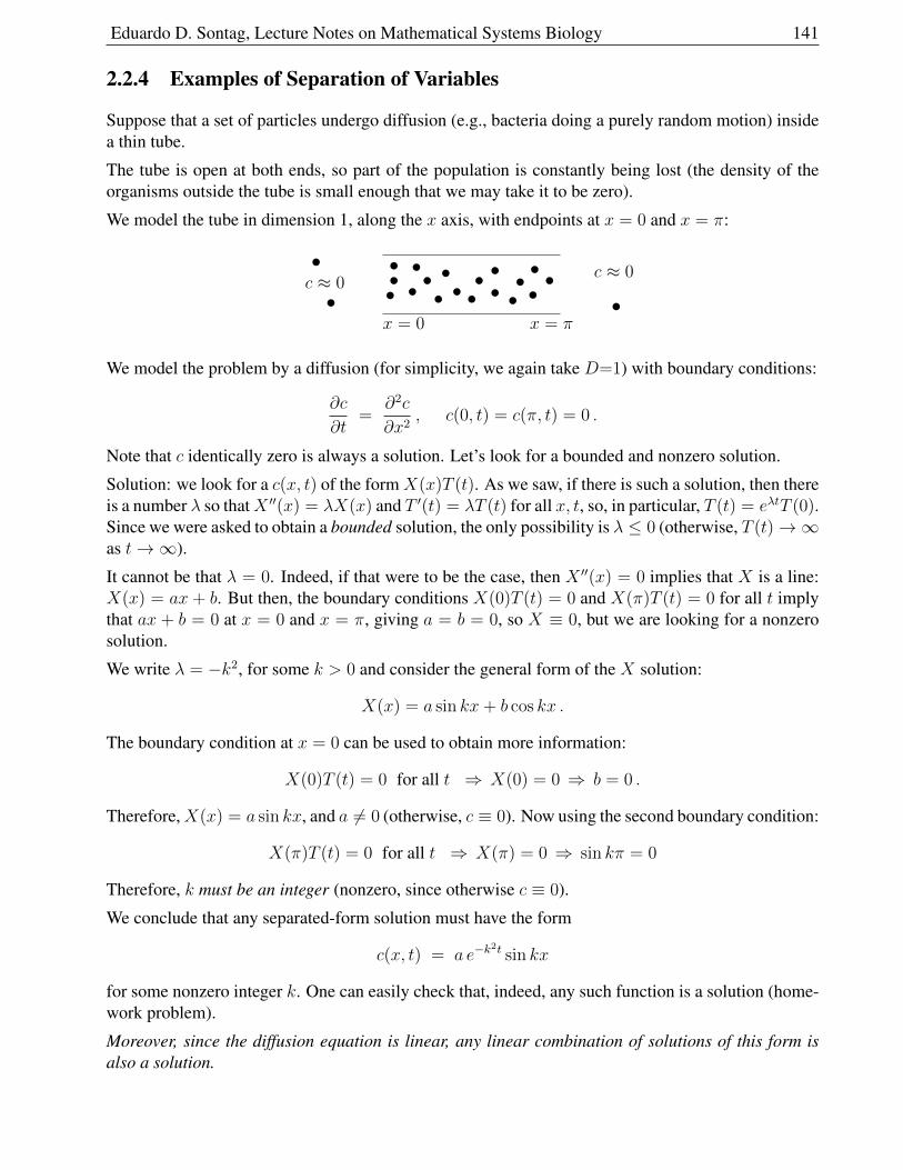
Eduardo D. Sontag, Lecture Notes on Mathematical Systems Biology 141
2.2.4 Examples of Separation of Variables
Suppose that a set of particles undergo diffusion (e.g., bacteria doing a purely random motion) insidea thin tube.
The tube is open at both ends, so part of the population is constantly being lost (the density of theorganisms outside the tube is small enough that we may take it to be zero).
We model the tube in dimension 1, along the x axis, with endpoints at x = 0 and x = π:
t t tt t tt tt ttt tttt tt t
tt
x = 0 x = π
c ≈ 0c ≈ 0
We model the problem by a diffusion (for simplicity, we again take D=1) with boundary conditions:
∂c
∂t=
∂2c
∂x2, c(0, t) = c(π, t) = 0 .
Note that c identically zero is always a solution. Let’s look for a bounded and nonzero solution.
Solution: we look for a c(x, t) of the formX(x)T (t). As we saw, if there is such a solution, then thereis a number λ so thatX ′′(x) = λX(x) and T ′(t) = λT (t) for all x, t, so, in particular, T (t) = eλtT (0).Since we were asked to obtain a bounded solution, the only possibility is λ ≤ 0 (otherwise, T (t)→∞as t→∞).
It cannot be that λ = 0. Indeed, if that were to be the case, then X ′′(x) = 0 implies that X is a line:X(x) = ax + b. But then, the boundary conditions X(0)T (t) = 0 and X(π)T (t) = 0 for all t implythat ax + b = 0 at x = 0 and x = π, giving a = b = 0, so X ≡ 0, but we are looking for a nonzerosolution.
We write λ = −k2, for some k > 0 and consider the general form of the X solution:
X(x) = a sin kx+ b cos kx .
The boundary condition at x = 0 can be used to obtain more information:
X(0)T (t) = 0 for all t ⇒ X(0) = 0 ⇒ b = 0 .
Therefore,X(x) = a sin kx, and a 6= 0 (otherwise, c ≡ 0). Now using the second boundary condition:
X(π)T (t) = 0 for all t ⇒ X(π) = 0 ⇒ sin kπ = 0
Therefore, k must be an integer (nonzero, since otherwise c ≡ 0).
We conclude that any separated-form solution must have the form
c(x, t) = a e−k2t sin kx
for some nonzero integer k. One can easily check that, indeed, any such function is a solution (home-work problem).
Moreover, since the diffusion equation is linear, any linear combination of solutions of this form isalso a solution.
Eduardo D. Sontag, Lecture Notes on Mathematical Systems Biology 142
For example,5e−9t sin 3x− 33e−16t sin 4x
is a solution of our problem.
In population problems, we cannot allow c to be negative. Solutions such as the above one are neg-ative when the trigonometric functions have negative values, so they are not physically meaningful.However, we could modify the problem by assuming, for example, that the density outside the tube isequal to some constantly maintained value, let is say, c = 100. Then, the PDE becomes
∂c
∂t=
∂2c
∂x2, c(0, t) = c(π, t) = 100 .
Since the PDE is linear, and since c(x, t) ≡ 100 is a solution, the function c(x, t) = c(x, t)− 100 is asolution of the homogeneous problem in which c(0, t) = c(π, t) = 0. Thus, c(x, t) = a e−k
2t sin kx isa solution of the homogeneous problem, which means that
c(x, t) = 100 + c(x, t) = 100 + a e−k2t sin kx
is a solution of the problem with boundary conditions = 100, for each a and each nonzero integerk. More generally, considering sums of the separated-form solutions, we have that if the sum of thecoefficients “a” is less than 100, then we are guaranteed that the solution stays always nonnegative.For example,
100 + 5e−9t sin 3x− 33e−16t sin 4x
solves the equation with boundary conditions c(0, t) = c(π, t) = 100 and is always nonnegative.
Fitting Initial Conditions
Next let’s add the requirement10 that the initial condition must be:
c(x, 0) = 3 sin 5x− 2 sin 8x .
Now, we know that any linear combination of the form∑k integer
ake−k2t sin kx
solves the equation. Since the initial condition has the two frequencies 5, 8, we should obviously tryfor a solution of the form:
c(x, t) = a5e−25t sin 5x+ a8e
−64t sin 8x .
We find the coefficients by plugging-in t = 0:
c(x, 0) = a5 sin 5x+ a8 sin 8x = 3 sin 5x− 2 sin 8x .
So we take a5 = 3 and a8 = −2; and thus obtain finally:
c(x, t) = 3e−25t sin 5x− 2e−64t sin 8x .
10For simplicity, we will take boundary conditions to be zero, even if this leads to physically meaningless negativesolutions; as earlier, we can simply add a constant to make the problem more realistic.
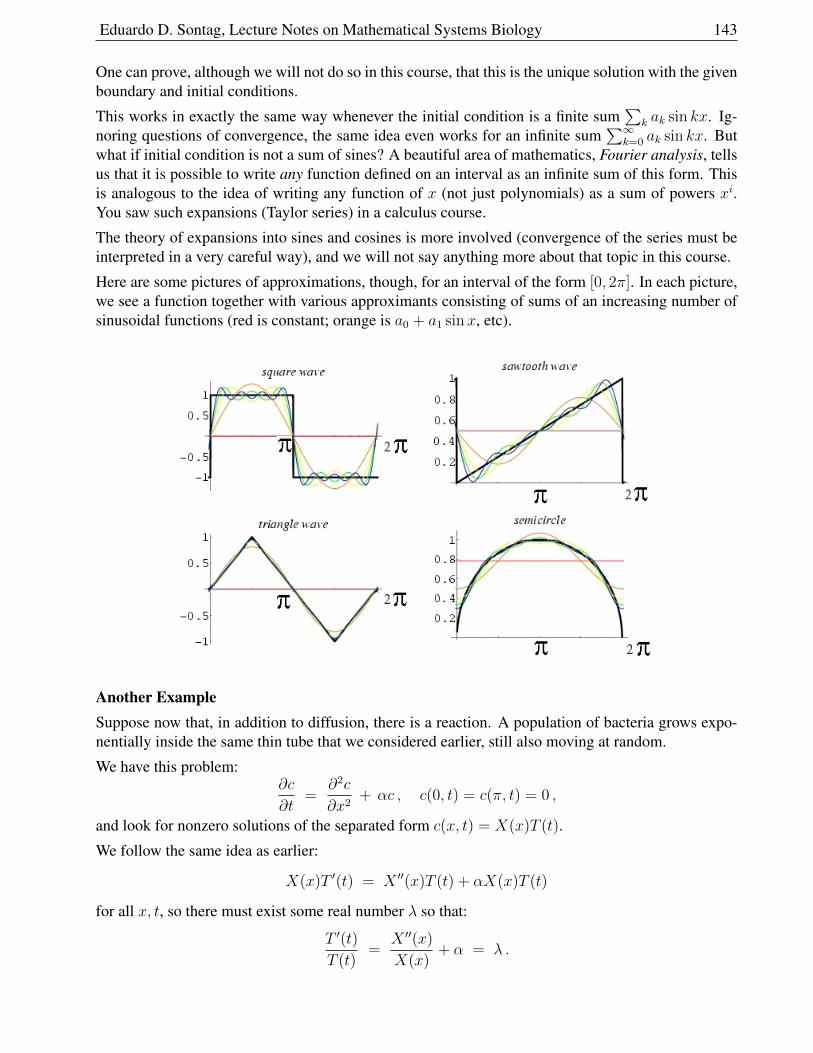
Eduardo D. Sontag, Lecture Notes on Mathematical Systems Biology 143
One can prove, although we will not do so in this course, that this is the unique solution with the givenboundary and initial conditions.
This works in exactly the same way whenever the initial condition is a finite sum∑
k ak sin kx. Ig-noring questions of convergence, the same idea even works for an infinite sum
∑∞k=0 ak sin kx. But
what if initial condition is not a sum of sines? A beautiful area of mathematics, Fourier analysis, tellsus that it is possible to write any function defined on an interval as an infinite sum of this form. Thisis analogous to the idea of writing any function of x (not just polynomials) as a sum of powers xi.You saw such expansions (Taylor series) in a calculus course.
The theory of expansions into sines and cosines is more involved (convergence of the series must beinterpreted in a very careful way), and we will not say anything more about that topic in this course.
Here are some pictures of approximations, though, for an interval of the form [0, 2π]. In each picture,we see a function together with various approximants consisting of sums of an increasing number ofsinusoidal functions (red is constant; orange is a0 + a1 sinx, etc).
Another ExampleSuppose now that, in addition to diffusion, there is a reaction. A population of bacteria grows expo-nentially inside the same thin tube that we considered earlier, still also moving at random.
We have this problem:∂c
∂t=
∂2c
∂x2+ αc , c(0, t) = c(π, t) = 0 ,
and look for nonzero solutions of the separated form c(x, t) = X(x)T (t).
We follow the same idea as earlier:
X(x)T ′(t) = X ′′(x)T (t) + αX(x)T (t)
for all x, t, so there must exist some real number λ so that:
T ′(t)
T (t)=
X ′′(x)
X(x)+ α = λ .
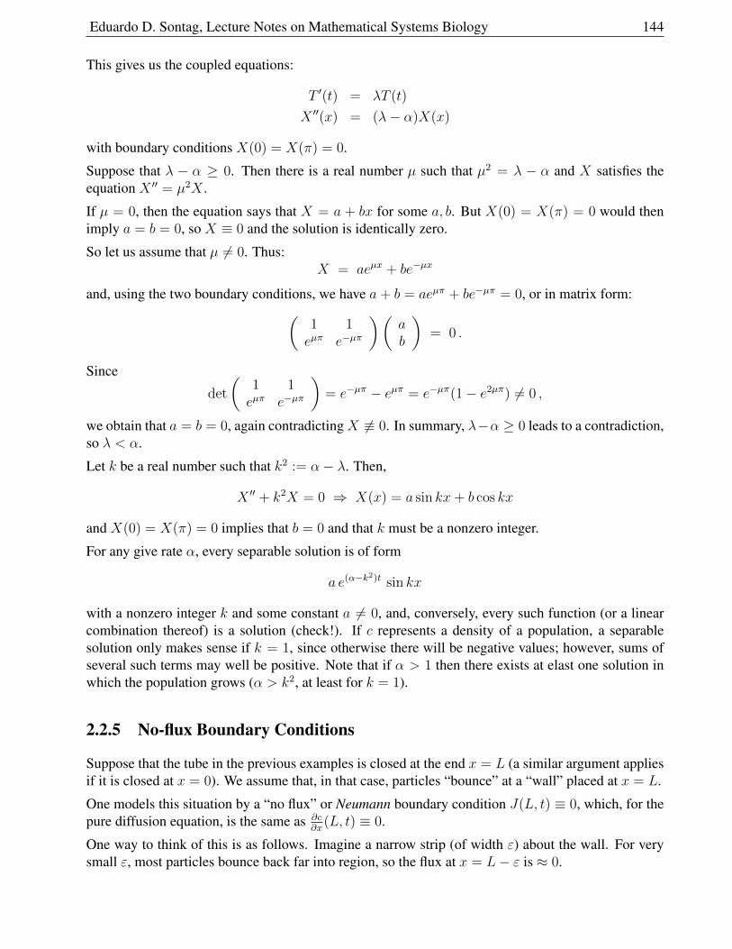
Eduardo D. Sontag, Lecture Notes on Mathematical Systems Biology 144
This gives us the coupled equations:
T ′(t) = λT (t)
X ′′(x) = (λ− α)X(x)
with boundary conditions X(0) = X(π) = 0.
Suppose that λ − α ≥ 0. Then there is a real number µ such that µ2 = λ − α and X satisfies theequation X ′′ = µ2X .
If µ = 0, then the equation says that X = a + bx for some a, b. But X(0) = X(π) = 0 would thenimply a = b = 0, so X ≡ 0 and the solution is identically zero.
So let us assume that µ 6= 0. Thus:X = aeµx + be−µx
and, using the two boundary conditions, we have a+ b = aeµπ + be−µπ = 0, or in matrix form:(1 1eµπ e−µπ
)(ab
)= 0 .
Since
det
(1 1eµπ e−µπ
)= e−µπ − eµπ = e−µπ(1− e2µπ) 6= 0 ,
we obtain that a = b = 0, again contradictingX 6≡ 0. In summary, λ−α ≥ 0 leads to a contradiction,so λ < α.
Let k be a real number such that k2 := α− λ. Then,
X ′′ + k2X = 0 ⇒ X(x) = a sin kx+ b cos kx
and X(0) = X(π) = 0 implies that b = 0 and that k must be a nonzero integer.
For any give rate α, every separable solution is of form
a e(α−k2)t sin kx
with a nonzero integer k and some constant a 6= 0, and, conversely, every such function (or a linearcombination thereof) is a solution (check!). If c represents a density of a population, a separablesolution only makes sense if k = 1, since otherwise there will be negative values; however, sums ofseveral such terms may well be positive. Note that if α > 1 then there exists at elast one solution inwhich the population grows (α > k2, at least for k = 1).
2.2.5 No-flux Boundary Conditions
Suppose that the tube in the previous examples is closed at the end x = L (a similar argument appliesif it is closed at x = 0). We assume that, in that case, particles “bounce” at a “wall” placed at x = L.
One models this situation by a “no flux” or Neumann boundary condition J(L, t) ≡ 0, which, for thepure diffusion equation, is the same as ∂c
∂x(L, t) ≡ 0.
One way to think of this is as follows. Imagine a narrow strip (of width ε) about the wall. For verysmall ε, most particles bounce back far into region, so the flux at x = L− ε is ≈ 0.
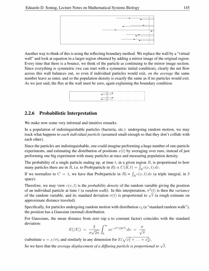
Eduardo D. Sontag, Lecture Notes on Mathematical Systems Biology 145
-
-
-
-
-
Another way to think of this is using the reflecting boundary method. We replace the wall by a “virtualwall” and look at equation in a larger region obtained by adding a mirror image of the original region.Every time that there is a bounce, we think of the particle as continuing to the mirror image section.Since everything is symmetric (we can start with a symmetric initial condition), clearly the net flowacross this wall balances out, so even if individual particles would exit, on the average the samenumber leave as enter, and so the population density is exactly the same as if no particles would exit.As we just said, the flux at the wall must be zero, again explaining the boundary condition.
--
2.2.6 Probabilistic Interpretation
We make now some very informal and intuitive remarks.
In a population of indistinguishable particles (bacteria, etc.) undergoing random motion, we maytrack what happens to each individual particle (assumed small enough so that they don’t collide witheach other).
Since the particles are indistinguishable, one could imagine performing a huge number of one-particleexperiments, and estimating the distribution of positions x(t) by averaging over runs, instead of justperforming one big experiment with many particles at once and measuring population density.
The probability of a single particle ending up, at time t, in a given region R, is proportional to howmany particles there are in R, i.e. to Prob(particle in R) ∝ C(R, t) =
∫Rc(x, t) dx.
If we normalize to C = 1, we have that Prob(particle in R) =∫Rc(x, t) dx (a triple integral, in 3
space).
Therefore, we may view c(x, t) is the probability density of the random variable giving the positionof an individual particle at time t (a random walk). In this interpretation, σ2(t) is then the varianceof the random variable, and its standard deviation σ(t) is proportional to
√t (a rough estimate on
approximate distance traveled).
Specifically, for particles undergoing random motion with distribution c0 (a “standard random walk”),the position has a Gaussian (normal) distribution.
For Gaussians, the mean distance from zero (up a to constant factor) coincides with the standarddeviation:
E(|X|) =2
σ√
2π
∫ ∞0
xe−x2/(2σ2) dx =
σ√π
(substitute u = x/σ), and similarly in any dimension for E(√x2
1 + . . .+ x2d).
So we have that the average displacement of a diffusing particle is proportional to√t.
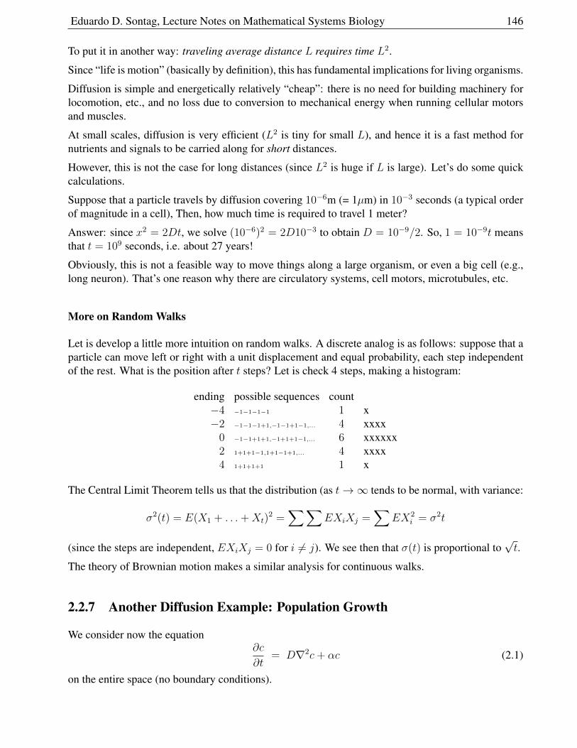
Eduardo D. Sontag, Lecture Notes on Mathematical Systems Biology 146
To put it in another way: traveling average distance L requires time L2.
Since “life is motion” (basically by definition), this has fundamental implications for living organisms.
Diffusion is simple and energetically relatively “cheap”: there is no need for building machinery forlocomotion, etc., and no loss due to conversion to mechanical energy when running cellular motorsand muscles.
At small scales, diffusion is very efficient (L2 is tiny for small L), and hence it is a fast method fornutrients and signals to be carried along for short distances.
However, this is not the case for long distances (since L2 is huge if L is large). Let’s do some quickcalculations.
Suppose that a particle travels by diffusion covering 10−6m (= 1µm) in 10−3 seconds (a typical orderof magnitude in a cell), Then, how much time is required to travel 1 meter?
Answer: since x2 = 2Dt, we solve (10−6)2 = 2D10−3 to obtain D = 10−9/2. So, 1 = 10−9t meansthat t = 109 seconds, i.e. about 27 years!
Obviously, this is not a feasible way to move things along a large organism, or even a big cell (e.g.,long neuron). That’s one reason why there are circulatory systems, cell motors, microtubules, etc.
More on Random Walks
Let is develop a little more intuition on random walks. A discrete analog is as follows: suppose that aparticle can move left or right with a unit displacement and equal probability, each step independentof the rest. What is the position after t steps? Let is check 4 steps, making a histogram:
ending possible sequences count−4 −1−1−1−1 1 x−2 −1−1−1+1,−1−1+1−1,... 4 xxxx
0 −1−1+1+1,−1+1+1−1,... 6 xxxxxx2 1+1+1−1,1+1−1+1,... 4 xxxx4 1+1+1+1 1 x
The Central Limit Theorem tells us that the distribution (as t→∞ tends to be normal, with variance:
σ2(t) = E(X1 + . . .+Xt)2 =
∑∑EXiXj =
∑EX2
i = σ2t
(since the steps are independent, EXiXj = 0 for i 6= j). We see then that σ(t) is proportional to√t.
The theory of Brownian motion makes a similar analysis for continuous walks.
2.2.7 Another Diffusion Example: Population Growth
We consider now the equation∂c
∂t= D∇2c+ αc (2.1)
on the entire space (no boundary conditions).
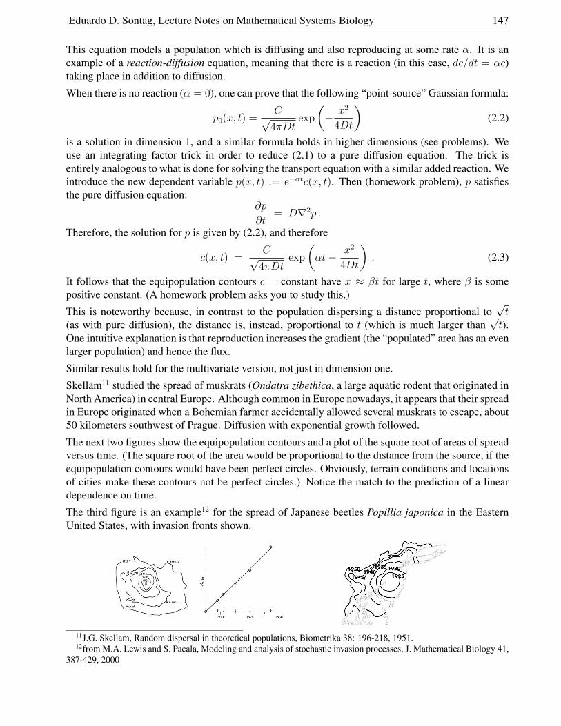
Eduardo D. Sontag, Lecture Notes on Mathematical Systems Biology 147
This equation models a population which is diffusing and also reproducing at some rate α. It is anexample of a reaction-diffusion equation, meaning that there is a reaction (in this case, dc/dt = αc)taking place in addition to diffusion.
When there is no reaction (α = 0), one can prove that the following “point-source” Gaussian formula:
p0(x, t) =C√
4πDtexp
(− x2
4Dt
)(2.2)
is a solution in dimension 1, and a similar formula holds in higher dimensions (see problems). Weuse an integrating factor trick in order to reduce (2.1) to a pure diffusion equation. The trick isentirely analogous to what is done for solving the transport equation with a similar added reaction. Weintroduce the new dependent variable p(x, t) := e−αtc(x, t). Then (homework problem), p satisfiesthe pure diffusion equation:
∂p
∂t= D∇2p .
Therefore, the solution for p is given by (2.2), and therefore
c(x, t) =C√
4πDtexp
(αt− x2
4Dt
). (2.3)
It follows that the equipopulation contours c = constant have x ≈ βt for large t, where β is somepositive constant. (A homework problem asks you to study this.)
This is noteworthy because, in contrast to the population dispersing a distance proportional to√t
(as with pure diffusion), the distance is, instead, proportional to t (which is much larger than√t).
One intuitive explanation is that reproduction increases the gradient (the “populated” area has an evenlarger population) and hence the flux.
Similar results hold for the multivariate version, not just in dimension one.
Skellam11 studied the spread of muskrats (Ondatra zibethica, a large aquatic rodent that originated inNorth America) in central Europe. Although common in Europe nowadays, it appears that their spreadin Europe originated when a Bohemian farmer accidentally allowed several muskrats to escape, about50 kilometers southwest of Prague. Diffusion with exponential growth followed.
The next two figures show the equipopulation contours and a plot of the square root of areas of spreadversus time. (The square root of the area would be proportional to the distance from the source, if theequipopulation contours would have been perfect circles. Obviously, terrain conditions and locationsof cities make these contours not be perfect circles.) Notice the match to the prediction of a lineardependence on time.
The third figure is an example12 for the spread of Japanese beetles Popillia japonica in the EasternUnited States, with invasion fronts shown.
11J.G. Skellam, Random dispersal in theoretical populations, Biometrika 38: 196-218, 1951.12from M.A. Lewis and S. Pacala, Modeling and analysis of stochastic invasion processes, J. Mathematical Biology 41,
387-429, 2000
Eduardo D. Sontag, Lecture Notes on Mathematical Systems Biology 148
Remark. Continuing on the topic of the Remark in page 128, suppose that each particle in a popula-tion evolves according to a differential equation dx/dt = f(x, t) +w, where “w” represents a “noise”effect which, in the absence of the f term, would make the particles undergo purely random motion,and the population density satisfies the diffusion equation with diffusion coefficient D. When botheffects are superimposed, we obtain, for the density, an equation like ∂c/∂t = −div (cf) + D∇2c.This is usually called a Fokker-Planck equation. (To be more precise, the Fokker-Planck equation de-scribes a more general situation, in which the “noise” term affects the dynamics in a way that dependson the current value of x. We’ll work out details in a future version of these notes.)
2.2.8 Systems of PDE’s
Of course, one often must study systems of partial differential equations, not just single PDE’s.
We just discuss one example, that of diffusion with growth and nutrient depletion, since the ideashould be easy to understand. This example nicely connects with the material that we started thecourse with.
We assume that a population of bacteria, with density n(x, t), move at random (diffusion), and in ad-dition also reproduce with a rate K(c(x, t)) that depends on the local concentration c(x, t) of nutrient.
The nutrient is depleted at a rate proportional to its use, and it itself diffuses. Finally, we assume thatthere is a linear death rate kn for the bacteria.
A model is:
∂n
∂t= Dn∇2n + (K(c)− k)n
∂c
∂t= Dc∇2c − αK(c)n
where Dn and Dc are diffusion constants. The function K(c) could be, for example, a Michaelis-Menten rate K(c) =
kmaxckn+c
You should ask yourself, as a homework problem, what the equations would be like if c were todenote, instead, a toxic agent, as well as formulate other variations of the idea.
Another example, related to this one, is that of chemotaxis with diffusion. We look at this examplelater, in the context of analyzing steady state solutions.
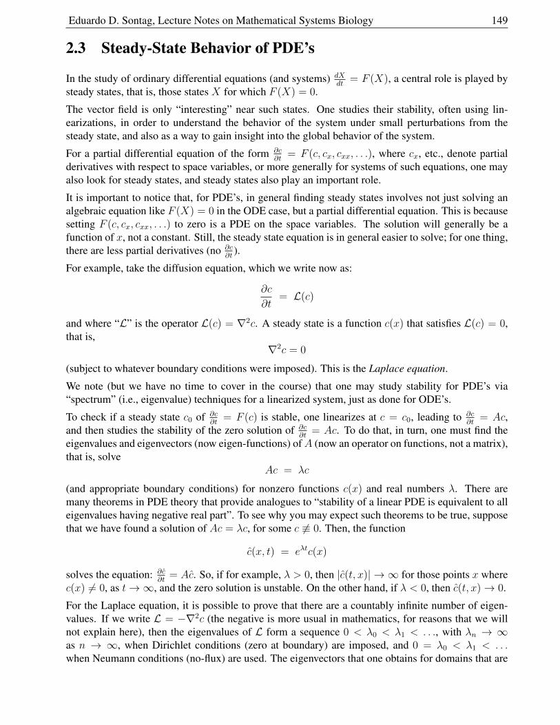
Eduardo D. Sontag, Lecture Notes on Mathematical Systems Biology 149
2.3 Steady-State Behavior of PDE’s
In the study of ordinary differential equations (and systems) dXdt
= F (X), a central role is played bysteady states, that is, those states X for which F (X) = 0.
The vector field is only “interesting” near such states. One studies their stability, often using lin-earizations, in order to understand the behavior of the system under small perturbations from thesteady state, and also as a way to gain insight into the global behavior of the system.
For a partial differential equation of the form ∂c∂t
= F (c, cx, cxx, . . .), where cx, etc., denote partialderivatives with respect to space variables, or more generally for systems of such equations, one mayalso look for steady states, and steady states also play an important role.
It is important to notice that, for PDE’s, in general finding steady states involves not just solving analgebraic equation like F (X) = 0 in the ODE case, but a partial differential equation. This is becausesetting F (c, cx, cxx, . . .) to zero is a PDE on the space variables. The solution will generally be afunction of x, not a constant. Still, the steady state equation is in general easier to solve; for one thing,there are less partial derivatives (no ∂c
∂t).
For example, take the diffusion equation, which we write now as:
∂c
∂t= L(c)
and where “L” is the operator L(c) = ∇2c. A steady state is a function c(x) that satisfies L(c) = 0,that is,
∇2c = 0
(subject to whatever boundary conditions were imposed). This is the Laplace equation.
We note (but we have no time to cover in the course) that one may study stability for PDE’s via“spectrum” (i.e., eigenvalue) techniques for a linearized system, just as done for ODE’s.
To check if a steady state c0 of ∂c∂t
= F (c) is stable, one linearizes at c = c0, leading to ∂c∂t
= Ac,and then studies the stability of the zero solution of ∂c
∂t= Ac. To do that, in turn, one must find the
eigenvalues and eigenvectors (now eigen-functions) ofA (now an operator on functions, not a matrix),that is, solve
Ac = λc
(and appropriate boundary conditions) for nonzero functions c(x) and real numbers λ. There aremany theorems in PDE theory that provide analogues to “stability of a linear PDE is equivalent to alleigenvalues having negative real part”. To see why you may expect such theorems to be true, supposethat we have found a solution of Ac = λc, for some c 6≡ 0. Then, the function
c(x, t) = eλtc(x)
solves the equation: ∂c∂t
= Ac. So, if for example, λ > 0, then |c(t, x)| → ∞ for those points x wherec(x) 6= 0, as t→∞, and the zero solution is unstable. On the other hand, if λ < 0, then c(t, x)→ 0.
For the Laplace equation, it is possible to prove that there are a countably infinite number of eigen-values. If we write L = −∇2c (the negative is more usual in mathematics, for reasons that we willnot explain here), then the eigenvalues of L form a sequence 0 < λ0 < λ1 < . . ., with λn → ∞as n → ∞, when Dirichlet conditions (zero at boundary) are imposed, and 0 = λ0 < λ1 < . . .when Neumann conditions (no-flux) are used. The eigenvectors that one obtains for domains that are
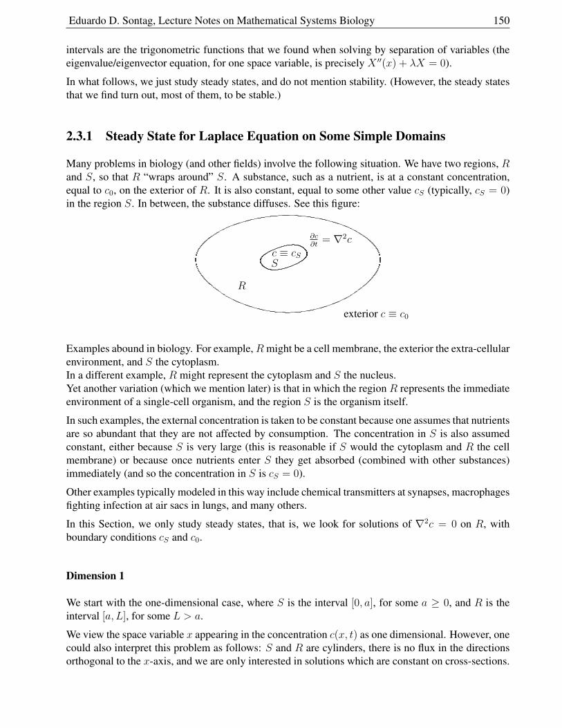
Eduardo D. Sontag, Lecture Notes on Mathematical Systems Biology 150
intervals are the trigonometric functions that we found when solving by separation of variables (theeigenvalue/eigenvector equation, for one space variable, is precisely X ′′(x) + λX = 0).
In what follows, we just study steady states, and do not mention stability. (However, the steady statesthat we find turn out, most of them, to be stable.)
2.3.1 Steady State for Laplace Equation on Some Simple Domains
Many problems in biology (and other fields) involve the following situation. We have two regions, Rand S, so that R “wraps around” S. A substance, such as a nutrient, is at a constant concentration,equal to c0, on the exterior of R. It is also constant, equal to some other value cS (typically, cS = 0)in the region S. In between, the substance diffuses. See this figure:
exterior c ≡ c0
∂c∂t
= ∇2cc ≡ cSS
R
Examples abound in biology. For example,Rmight be a cell membrane, the exterior the extra-cellularenvironment, and S the cytoplasm.In a different example, R might represent the cytoplasm and S the nucleus.Yet another variation (which we mention later) is that in which the region R represents the immediateenvironment of a single-cell organism, and the region S is the organism itself.
In such examples, the external concentration is taken to be constant because one assumes that nutrientsare so abundant that they are not affected by consumption. The concentration in S is also assumedconstant, either because S is very large (this is reasonable if S would the cytoplasm and R the cellmembrane) or because once nutrients enter S they get absorbed (combined with other substances)immediately (and so the concentration in S is cS = 0).
Other examples typically modeled in this way include chemical transmitters at synapses, macrophagesfighting infection at air sacs in lungs, and many others.
In this Section, we only study steady states, that is, we look for solutions of ∇2c = 0 on R, withboundary conditions cS and c0.
Dimension 1
We start with the one-dimensional case, where S is the interval [0, a], for some a ≥ 0, and R is theinterval [a, L], for some L > a.
We view the space variable x appearing in the concentration c(x, t) as one dimensional. However, onecould also interpret this problem as follows: S and R are cylinders, there is no flux in the directionsorthogonal to the x-axis, and we are only interested in solutions which are constant on cross-sections.
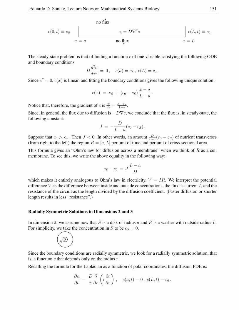
Eduardo D. Sontag, Lecture Notes on Mathematical Systems Biology 151
6
?
c(0, t) ≡ cS
no flux
no flux
c(L, t) ≡ c0
x = a x = L
ct = D∇2c
The steady-state problem is that of finding a function c of one variable satisfying the following ODEand boundary conditions:
Dd2c
dx2= 0 , c(a) = cS , c(L) = c0 .
Since c′′ = 0, c(x) is linear, and fitting the boundary conditions gives the following unique solution:
c(x) = cS + (c0 − cS)x− aL− a
.
Notice that, therefore, the gradient of c is dcdx
= c0−cSL−a .
Since, in general, the flux due to diffusion is −D∇c, we conclude that the flux is, in steady-state, thefollowing constant:
J = − D
L− a(c0 − cS) .
Suppose that c0 > cS . Then J < 0. In other words, an amount DL−a(c0 − cS) of nutrient transverses
(from right to the left) the region R = [a, L] per unit of time and per unit of cross-sectional area.
This formula gives an “Ohm’s law for diffusion across a membrane” when we think of R as a cellmembrane. To see this, we write the above equality in the following way:
cS − c0 = JL− aD
which makes it entirely analogous to Ohm’s law in electricity, V = IR. We interpret the potentialdifference V as the difference between inside and outside concentrations, the flux as current I , and theresistance of the circuit as the length divided by the diffusion coefficient. (Faster diffusion or shorterlength results in less “resistance”.)
Radially Symmetric Solutions in Dimensions 2 and 3
In dimension 2, we assume now that S is a disk of radius a and R is a washer with outside radius L.For simplicity, we take the concentration in S to be cS = 0.
kSR&%'$
Since the boundary conditions are radially symmetric, we look for a radially symmetric solution, thatis, a function c that depends only on the radius r.
Recalling the formula for the Laplacian as a function of polar coordinates, the diffusion PDE is:
∂c
∂t=
D
r
∂
∂r
(r∂c
∂r
), c(a, t) = 0 , c(L, t) = c0 .
Eduardo D. Sontag, Lecture Notes on Mathematical Systems Biology 152
Since we are looking only for a steady-state solution, we set the right-hand side to zero and look forc = c(r) such that
(rc′)′ = 0 c(a) = 0 , c(L) = c0 ,
where prime indicates derivative with respect to r.
A homework problem asks to show that the radially symmetric solution for the washer is:
c(r) = c0ln(r/a)
ln(L/a).
Similarly, in dimension 3, taking S as a ball of radius a and R as the spherical shell with inside radiusa and outside radius L, we have:
∂c
∂t=
D
r2
∂
∂r
(r2 ∂c
∂r
), c(t, a) = 0 , c(L, t) = c0
The solution for the spherical shell is (homework problem):
c(r) =Lc0
L− a
(1− a
r
).
Notice the different forms of the solutions in dimensions 1, 2, and 3.
In the dimension 3 case, the derivative of c in the radial direction is, therefore:
c′(r) =Lc0a
(L− a)r2.
We now specialize to the example in which the region R represents the environment surrounding asingle-cell organism, the region S is the organism itself, and c models nutrient concentration.
We assume that the concentration of nutrient is constant far away from the organism, let us say fartherthan distance L, and L a.
Then c′(r) = c0a(1−a/L)r2
≈ c0ar2
.
In general, the steady-state flux due to diffusion, in the radial direction, is −Dc′(r). In particular, onthe boundary of S, where r = a, we have:
J = −Dc0
a.
Thus −J is the amount of nutrient that passes, in steady state, through each unit of area of the bound-ary, per unit of time. (The negative sign because the flow is toward the inside, i.e. toward smaller r,since J < 0.)
Since the boundary of S is a sphere of radius a, it has surface area 4πa2. Therefore, nutrients enter Sat a rate of
Dc0
a× 4πa2 = 4πDc0a
per unit of time.
Eduardo D. Sontag, Lecture Notes on Mathematical Systems Biology 153
On the other hand, the metabolic need is roughly proportional to the volume of the organism. Thus,the amount of nutrients needed per unit of time is:
4
3πa3M ,
where M is the metabolic rate per unit of volume per unit of time.
For the organism to survive, enough nutrients must pass through its boundary. If diffusion is the onlymechanism for nutrients to come in, then survivability imposes the following constraint:
4πDc0a ≥4
3πa3M ,
that is,
a ≤ acritical =
√3Dc0
M.
Phytoplankton13 are free-floating aquatic organisms, and use bicarbonate ions (which enter by diffu-sion) as a source of carbon for photosynthesis, consuming one mole of bicarbonate per second percubic meter of cell. The concentration of bicarbonate in seawater is about 1.5 moles per cubic meter,and D ≈ 1.5× 10⁻⁹m2s−1. This gives
acritical =√
3× 1.5× 10−9 × 1.5m2 ≈ 82× 10−6m = 82µm (microns) .
This is, indeed, about the size of a typical “diatom” in the sea.
Larger organisms must use active transport mechanisms to ingest nutrients!
2.3.2 Steady States for a Diffusion/Chemotaxis Model
A very often used model that combines diffusion and chemotaxis is due to Keller and Segel. Themodel simply adds the diffusion and chemotaxis fluxes. In dimension 1, we have, then:
∂c
∂t= −div J = − ∂
∂x
(α c V ′ −D∂c
∂x
).
We assume that the bacteria live on the one-dimensional interval [0, L] and that no bacteria can enteror leave through the endpoints. That is, we have no flux on the boundary:14
J(0, t) = J(L, t) = 0 ∀ t .
Let us find the steady states.15
13We borrow this example from M. Denny and S. Gaines, Chance in Biology, Princeton University Press, 2000. Theauthors point out there that the metabolic need is more accurately proportional, for multicellular organisms, to (mass)3/4,but it is not so clear what the correct scaling law is for unicellular ones.
14Notice that this is not the same as asking that ∂c∂x (0, t) = ∂c∂x (L, t) = 0. The density might be constant near a boundary,
but this does not mean that the population will not get redistributed, since there is also movement due to chemotaxis. Onlyfor a pure diffusion, when J = −D ∂c
∂x , is no-flux the same as ∂c∂x = 0.
15Note that, for a model in which there is only chemotaxis, there cannot be any stedy states, unless V was constant -why?
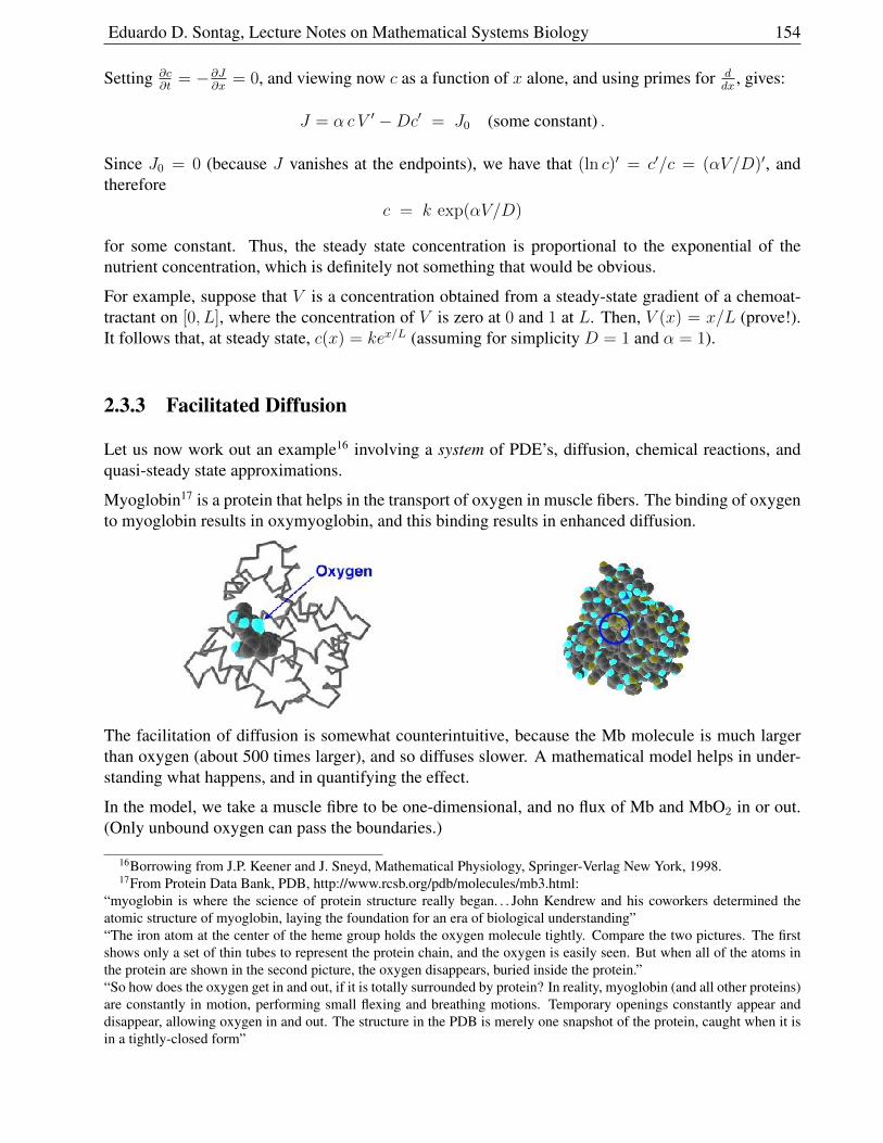
Eduardo D. Sontag, Lecture Notes on Mathematical Systems Biology 154
Setting ∂c∂t
= −∂J∂x
= 0, and viewing now c as a function of x alone, and using primes for ddx
, gives:
J = α c V ′ −Dc′ = J0 (some constant) .
Since J0 = 0 (because J vanishes at the endpoints), we have that (ln c)′ = c′/c = (αV/D)′, andtherefore
c = k exp(αV/D)
for some constant. Thus, the steady state concentration is proportional to the exponential of thenutrient concentration, which is definitely not something that would be obvious.
For example, suppose that V is a concentration obtained from a steady-state gradient of a chemoat-tractant on [0, L], where the concentration of V is zero at 0 and 1 at L. Then, V (x) = x/L (prove!).It follows that, at steady state, c(x) = kex/L (assuming for simplicity D = 1 and α = 1).
2.3.3 Facilitated Diffusion
Let us now work out an example16 involving a system of PDE’s, diffusion, chemical reactions, andquasi-steady state approximations.
Myoglobin17 is a protein that helps in the transport of oxygen in muscle fibers. The binding of oxygento myoglobin results in oxymyoglobin, and this binding results in enhanced diffusion.
The facilitation of diffusion is somewhat counterintuitive, because the Mb molecule is much largerthan oxygen (about 500 times larger), and so diffuses slower. A mathematical model helps in under-standing what happens, and in quantifying the effect.
In the model, we take a muscle fibre to be one-dimensional, and no flux of Mb and MbO2 in or out.(Only unbound oxygen can pass the boundaries.)
16Borrowing from J.P. Keener and J. Sneyd, Mathematical Physiology, Springer-Verlag New York, 1998.17From Protein Data Bank, PDB, http://www.rcsb.org/pdb/molecules/mb3.html:
“myoglobin is where the science of protein structure really began. . . John Kendrew and his coworkers determined theatomic structure of myoglobin, laying the foundation for an era of biological understanding”“The iron atom at the center of the heme group holds the oxygen molecule tightly. Compare the two pictures. The firstshows only a set of thin tubes to represent the protein chain, and the oxygen is easily seen. But when all of the atoms inthe protein are shown in the second picture, the oxygen disappears, buried inside the protein.”“So how does the oxygen get in and out, if it is totally surrounded by protein? In reality, myoglobin (and all other proteins)are constantly in motion, performing small flexing and breathing motions. Temporary openings constantly appear anddisappear, allowing oxygen in and out. The structure in the PDB is merely one snapshot of the protein, caught when it isin a tightly-closed form”
Eduardo D. Sontag, Lecture Notes on Mathematical Systems Biology 155
s(0, t) ≡ s0 s(L, 0) ≡ sL s0
x = 0 x = L
s = O2, e = Mb, c = MbO2
The chemical reaction is just that of binding and unbinding:
O2 +Mbk+−→←−k−
MbO2
with equations:
∂s
∂t= Ds
∂2s
∂x2+ k−c− k+se
∂e
∂t= De
∂2e
∂x2+ k−c− k+se
∂c
∂t= Dc
∂2c
∂x2− k−c+ k+se ,
where we assume that De = Dc (since Mb and MbO2 have comparable sizes). The boundary condi-tions are ∂e
∂x= ∂c
∂x≡ 0 at x = 0, L, and s(0) = s0, s(L) = sL.
We next do a steady-state analysis of this problem, setting:
Dssxx + k−c− k+se = 0
Deexx + k−c− k+se = 0
Dccxx − k−c+ k+se = 0
Since De = Dc, we have that (e+ c)xx ≡ 0.So, e+ c is a linear function of x, whose derivative is zero at the boundaries (no flux).Therefore, e+ c is constant, let us say equal to e0.
On the other hand, adding the first and third equations gives us that
(Dssx +Dccx)x = Dssxx +Dccxx = 0 .
This means that Dssx +Dccx is also constant:
Dssx +Dccx = −J .
Observe that J is the the total flux of oxygen (bound or not), since it is the sum of the fluxes −Dssxof s = O2 and −Dccx of c = MbO2.
Let f(x) = Dss(x) +Dcc(x). Since f ′ = −J , it follows that f(0)− f(L) = JL, which means:
J =Ds
L(s0 − sL) +
Dc
L(c0 − cL)
(where one knows the oxygen concentrations s0 and sL, but not necessarily c0 and cL).
We will next do a quasi-steady state approximation, under the hypothesis that Ds is very small com-pared to the other numbers appearing in:
Dssxx + k−c− k+s(e0 − c) = 0
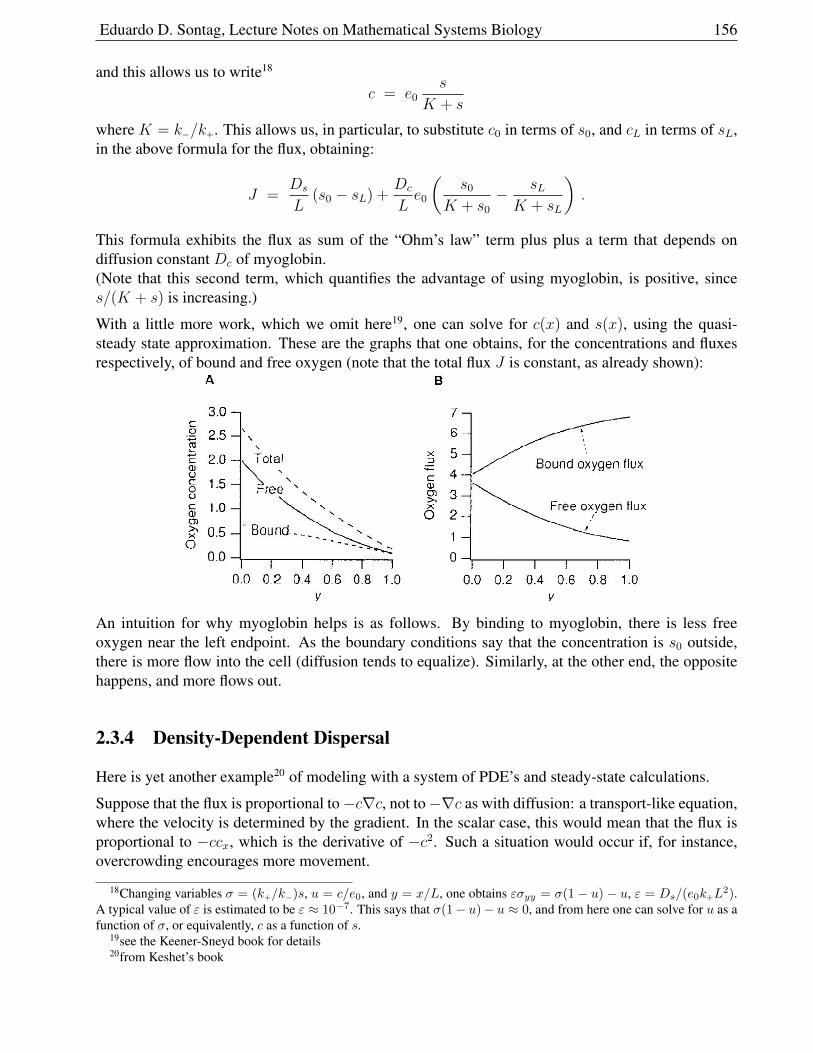
Eduardo D. Sontag, Lecture Notes on Mathematical Systems Biology 156
and this allows us to write18
c = e0s
K + s
where K = k−/k+. This allows us, in particular, to substitute c0 in terms of s0, and cL in terms of sL,in the above formula for the flux, obtaining:
J =Ds
L(s0 − sL) +
Dc
Le0
(s0
K + s0
− sLK + sL
).
This formula exhibits the flux as sum of the “Ohm’s law” term plus plus a term that depends ondiffusion constant Dc of myoglobin.(Note that this second term, which quantifies the advantage of using myoglobin, is positive, sinces/(K + s) is increasing.)
With a little more work, which we omit here19, one can solve for c(x) and s(x), using the quasi-steady state approximation. These are the graphs that one obtains, for the concentrations and fluxesrespectively, of bound and free oxygen (note that the total flux J is constant, as already shown):
An intuition for why myoglobin helps is as follows. By binding to myoglobin, there is less freeoxygen near the left endpoint. As the boundary conditions say that the concentration is s0 outside,there is more flow into the cell (diffusion tends to equalize). Similarly, at the other end, the oppositehappens, and more flows out.
2.3.4 Density-Dependent Dispersal
Here is yet another example20 of modeling with a system of PDE’s and steady-state calculations.
Suppose that the flux is proportional to−c∇c, not to−∇c as with diffusion: a transport-like equation,where the velocity is determined by the gradient. In the scalar case, this would mean that the flux isproportional to −ccx, which is the derivative of −c2. Such a situation would occur if, for instance,overcrowding encourages more movement.
18Changing variables σ = (k+/k−)s, u = c/e0, and y = x/L, one obtains εσyy = σ(1− u)− u, ε = Ds/(e0k+L2).
A typical value of ε is estimated to be ε ≈ 10−7. This says that σ(1− u)− u ≈ 0, and from here one can solve for u as afunction of σ, or equivalently, c as a function of s.
19see the Keener-Sneyd book for details20from Keshet’s book
Eduardo D. Sontag, Lecture Notes on Mathematical Systems Biology 157
So we have∂u
∂t= −div (−αu∇u)
and, in particular, in dimension 1:∂u
∂t= α
∂
∂x
(u∂u
∂x
)Let us look for steady states: u = u(x) solving (with u′ = ∂u
∂x):
(uu′)′ = 0 .
This means that (u2)′′ = 0, i.e. u(x)2 = ax+ b, or u(x) =√ax+ b for some constants a, b. Suppose
that we also impose boundary conditions u(0) = 1 and u(1) = 2. Then, u(x) =√
3x+ 1. The plot ofu(x) clearly shows that the total amount of individuals (the integral
∫ 1
0u(x)dx) is larger than it would
be if pure diffusion would occur, in which case u(x) = x+ 1 (why?).
To make the problem a little more interesting, let us now assume that there are two interacting popu-lations, with densities u and v respectively, and each moves with a velocity that is proportional to thegradient of the total population u+ v.
We obtain these equations:
∂u
∂t= −div (−αu∇(u+ v))
∂v
∂t= −div (−βv∇(u+ v))
and, in particular, in dimension 1:
∂u
∂t= α
∂
∂x
(u∂(u+ v)
∂x
)∂v
∂t= β
∂
∂x
(v∂(u+ v)
∂x
).
Let us look for steady states: u = u(x) and v = v(x) solving (with u′ = ∂u∂x
, v′ = ∂v∂x
):
(u(u+ v)′)′ = (v(u+ v)′)′ = 0 .
There must exist constants c1, c2 so that:
u(u+ v)′ = c1 , v(u+ v)′ = c2 .
We study three separate cases:(1) c1 = c2 = 0(2) c2 6= 0 and c1 = 0,(3) c1c2 6= 0(the case c1 6= 0 and c2 = 0 is similar to (2)).
Case (1):here [(u + v)2]′ = 2(u + v)(u + v)′ = 2u(u + v)′ + 2v(u + v)′ = 0, so u + v is constant. That’s thebest that we can say.
Eduardo D. Sontag, Lecture Notes on Mathematical Systems Biology 158
Case (2):
c2 6= 0 ⇒ v(x) 6= 0, (u+ v)′(x) 6= 0 ∀x .
Also,c1 = 0 ⇒ u ≡ 0 ⇒ vv′ ≡ c2 ⇒ (v2)′ ≡ 2c2
implies v2 = 2c2x+K for some constant K, so (taking the positive square root, because v ≥ 0, beinga population):
v =√
2c2x+K , u ≡ 0 .
Case (3):Necessarily u(x) 6= 0 and v(x) 6= 0 for all x, so can divide and obtain:
(u+ v)′ =c1
u=c2
v.
Hence u = (c1/c2)v can be substituted into u′ + v′ = c2v
to obtain (1 + c1/c2)v′ = c2/v, i.e. vv′ =c2/(1 + c1/c2), or (v2)′ = 2c2/(1 + c1/c2), from which:
v2(x) =2c2x
1 + c1/c2
+K
for some K, and so:
v(x) =
(2c2x
1 + c2/c1
+K
)1/2
.
Since u = (c1/c2)v,
u(x) =
(2c1x
1 + c1/c2
+Kc21/c
22
)1/2
.
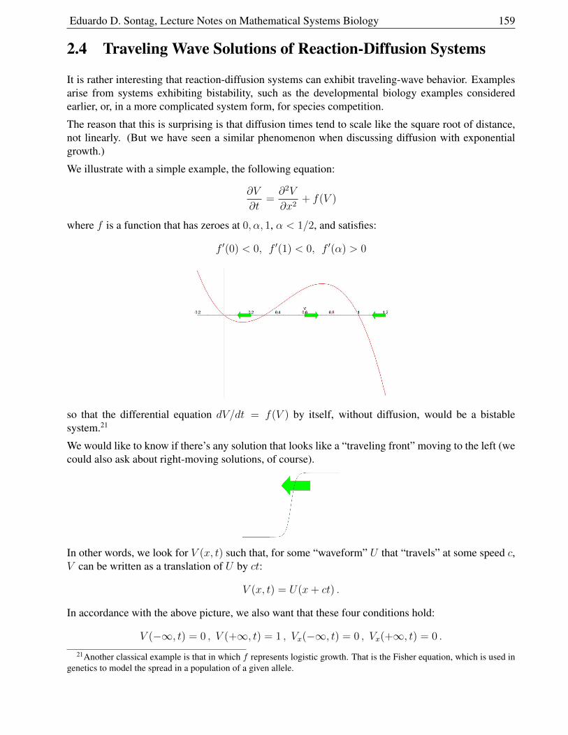
Eduardo D. Sontag, Lecture Notes on Mathematical Systems Biology 159
2.4 Traveling Wave Solutions of Reaction-Diffusion Systems
It is rather interesting that reaction-diffusion systems can exhibit traveling-wave behavior. Examplesarise from systems exhibiting bistability, such as the developmental biology examples consideredearlier, or, in a more complicated system form, for species competition.
The reason that this is surprising is that diffusion times tend to scale like the square root of distance,not linearly. (But we have seen a similar phenomenon when discussing diffusion with exponentialgrowth.)
We illustrate with a simple example, the following equation:
∂V
∂t=∂2V
∂x2+ f(V )
where f is a function that has zeroes at 0, α, 1, α < 1/2, and satisfies:
f ′(0) < 0, f ′(1) < 0, f ′(α) > 0
so that the differential equation dV/dt = f(V ) by itself, without diffusion, would be a bistablesystem.21
We would like to know if there’s any solution that looks like a “traveling front” moving to the left (wecould also ask about right-moving solutions, of course).
In other words, we look for V (x, t) such that, for some “waveform” U that “travels” at some speed c,V can be written as a translation of U by ct:
V (x, t) = U(x+ ct) .
In accordance with the above picture, we also want that these four conditions hold:
V (−∞, t) = 0 , V (+∞, t) = 1 , Vx(−∞, t) = 0 , Vx(+∞, t) = 0 .
21Another classical example is that in which f represents logistic growth. That is the Fisher equation, which is used ingenetics to model the spread in a population of a given allele.
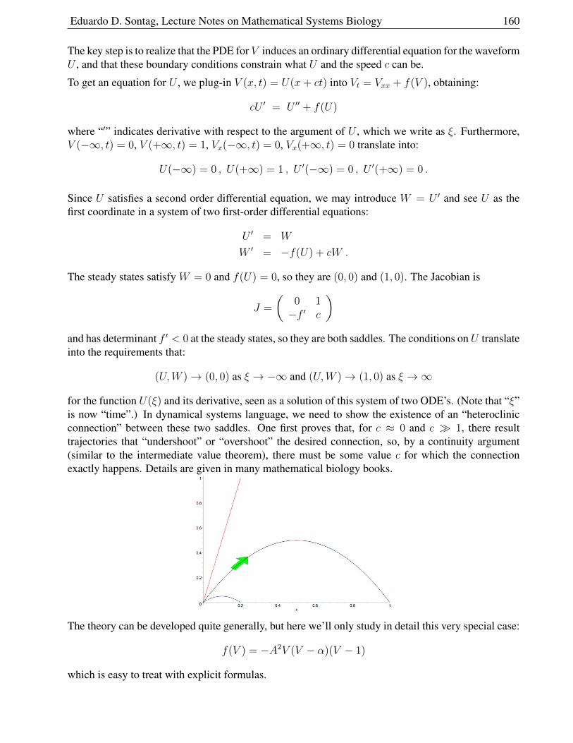
Eduardo D. Sontag, Lecture Notes on Mathematical Systems Biology 160
The key step is to realize that the PDE for V induces an ordinary differential equation for the waveformU , and that these boundary conditions constrain what U and the speed c can be.
To get an equation for U , we plug-in V (x, t) = U(x+ ct) into Vt = Vxx + f(V ), obtaining:
cU ′ = U ′′ + f(U)
where “′” indicates derivative with respect to the argument of U , which we write as ξ. Furthermore,V (−∞, t) = 0, V (+∞, t) = 1, Vx(−∞, t) = 0, Vx(+∞, t) = 0 translate into:
U(−∞) = 0 , U(+∞) = 1 , U ′(−∞) = 0 , U ′(+∞) = 0 .
Since U satisfies a second order differential equation, we may introduce W = U ′ and see U as thefirst coordinate in a system of two first-order differential equations:
U ′ = W
W ′ = −f(U) + cW .
The steady states satisfy W = 0 and f(U) = 0, so they are (0, 0) and (1, 0). The Jacobian is
J =
(0 1−f ′ c
)and has determinant f ′ < 0 at the steady states, so they are both saddles. The conditions on U translateinto the requirements that:
(U,W )→ (0, 0) as ξ → −∞ and (U,W )→ (1, 0) as ξ →∞
for the function U(ξ) and its derivative, seen as a solution of this system of two ODE’s. (Note that “ξ”is now “time”.) In dynamical systems language, we need to show the existence of an “heteroclinicconnection” between these two saddles. One first proves that, for c ≈ 0 and c 1, there resulttrajectories that “undershoot” or “overshoot” the desired connection, so, by a continuity argument(similar to the intermediate value theorem), there must be some value c for which the connectionexactly happens. Details are given in many mathematical biology books.
The theory can be developed quite generally, but here we’ll only study in detail this very special case:
f(V ) = −A2V (V − α)(V − 1)
which is easy to treat with explicit formulas.
Eduardo D. Sontag, Lecture Notes on Mathematical Systems Biology 161
Since U will satisfy U ′ = 0 when U = 0, 1, we guess the functional relation:
U ′(ξ) = BU(ξ) (1− U(ξ))
(note that we are looking for a U satisfying 0 ≤ U ≤ 1, so 1−U ≥ 0). We write “ξ” for the argumentof U so as to not confuse it with x.
We substitute U ′ = BU(1− U) and (taking derivatives of this expression)
U ′′ = B2U(1− U)(1− 2U)
into the differential equation cU ′ = U ′′ +A2U(U − α)(U − 1), and cancel U(U − 1), obtaining (thecalculation is given as a homework problem):
B2(2U − 1) + cB − A2(U − α) = 0 .
Since U is not constant (because U(−∞) = 0 and U(+∞) = 1), this means that we can comparecoefficients of U in this expression, and conclude: that 2B2 − A2 = 0 and −B2 + cB + αA2 = 0.Therefore:
B = A/√
2 , c =(1− 2α)A√
2.
Substituting back into the differential equation for U , we have:
U ′ = BU(1− U) =A√2U(1− U) ,
an ODE that now does not involve the unknown B. We solve this ODE by separation of variables andpartial fractions, using for example U(0) = 1/2 as an initial condition, getting:
U(ξ) =1
2
[1 + tanh
(A
2√
2ξ
)](a homework problem asks to verify that this is a solution). Finally, since V (x, t) = U(x + ct), weconclude that:
V (x, t) =1
2
[1 + tanh
(A
2√
2(x+ ct)
)]where c = (1−2α)A√
2.
Observe that the speed c was uniquely determined; it will be larger if α ≈ 0, or if the reaction isstronger (larger A). This is not surprising! (Why?)
Eduardo D. Sontag, Lecture Notes on Mathematical Systems Biology 162
2.5 Problems for PDE chapter
2.5.1 Transport problems
1. Suppose that c(x, t) is the density of bacteria (in one space dimension) being carried east by awind blowing at 1 mph. The bacteria double every 1 hour. Suppose that we know that c(1, t) = tfor all t. Derive a formula for c(x, t) for all x, t, by using the general form “eλtf(x− vt)” anddetermining the constant λ and the function f from the given information. You should end upwith this answer:
(1− x+ t) et ln 2 e−(ln 2)(1−x+t)
but do not just plug-in this expression to verify that it is a solution, since the whole point of theproblem is for you to be able to work out the problem without knowing the solution!
2. Suppose that a population, with density c(x, t) (in one dimension), is being transported withvelocity v = 5x. That is to say, the velocity is not constant, but it depends on the position x.(This could happen, for example, if wind is dispersing the population, but the wind speed is noteverywhere the same.) There are no additional growth or decay, diffusion, chemotaxis, etc., justpure transport. Circle which of the following PDE’s describes the evolution of c:
∂c
∂t=−x ∂c
∂x
∂c
∂t=−5c
∂c
∂t=−5x
∂c
∂x
∂c
∂t=−5c− x ∂c
∂x
∂c
∂t=−5− ∂c
∂x∂c
∂t=−c− x ∂c
∂x
∂c
∂t=−5c− 5x
∂c
∂x
∂c
∂t=−5c− 5
∂c
∂x
∂c
∂t=−5c− 5V ′
∂c
∂x(none of these)
3. Suppose that a population, with density c(x, t) (in one dimension), is being transported withvelocity v = 5. There is no additional growth or decay, diffusion, chemotaxis, etc., just puretransport. The initial density is c(x, 0)=x2/(1 + x2).
(a) Give a formula for c(x, t).
(b) The density at position x=12 at time t=2 is (circle the right one):
0 0.1 0.2 0.3 0.4 0.5 0.6 0.7 0.8 0.9 (none of these)
4. Suppose that c(x, t) is the density of radioactive particles (in one space dimension) being carriedeast by a wind blowing at 6 mph. The particles decay with a half-life of 4 hours. Suppose thatwe know that c(1, t) = 1
1+tfor all t. Find c(x, t) for all x, t.
5. Suppose that a population, with density c(x, t) (in one dimension), is being transported withvelocity v = 1. There is no additional growth or decay, diffusion, chemotaxis, etc., just puretransport. At time t = 1, the density is c(x, 1)=x2−2x+ 1. (Please note that we didn’t specifyinitial conditions at “t=0”.)
(a) Give a formula for c(x, t).
(b) (2) The density at position x=1 at time t=2 is (circle the right one):
0 -27 -17 1 -1 2 -2 3 -3 4 -4 27 (none of these)
Eduardo D. Sontag, Lecture Notes on Mathematical Systems Biology 163
6. Suppose that a population, with density c(x, t) (in one dimension), is being transported withvelocity v = 5. There are no additional growth or decay, diffusion, chemotaxis, etc., just puretransport. The initial density is c(x, 0)=x2/(1 + x2).
(a) Give a formula for c(x, t).
(b) The density at position x=12 at time t=2 is (circle the right one):
0 0.1 0.2 0.3 0.4 0.5 0.6 0.7 0.8 0.9 (none of these)
7. Suppose c(x, t) is the density of bacterial population being carried east by a wind blowing at 4mph. The bacteria reproduce exponentially, with a doubling time of 5 hours.
(a) Find the density c(x, t) in each of these cases:(1) c(x, 0) ≡ 1 (2) c(x, 0) = 2 + cosx (3) c(x, 0) = 1
1+x2(4) c(x, 1) =
2 + cos x(5) c(0, t) ≡ 1 (6) c(0, t) = sin t (7) c(1, t) = 1
1+et.
(b) Sketch the density c(x, 10) at time t = 10.
8. Prove the following analog in dimension 3 of the theorem on solutions of the transport equation(the constant velocity v is now a vector): c(x, y, z, t) = f(x− v1t, y− v2t, z − v3t)e
−λt. (Hint:use α(x, y, z, t) = c(x+ v1t, y + v2t, z + v3t, t).)
2.5.2 Chemotaxis problems
1. Give an example of an equation that would model this situation: the speed of movement isan increasing function of the norm of the gradient, but is bounded by some maximal possiblespeed.
2. We are given this chemotaxis equation (one space dimension) for the concentration of a mi-croorganism (assuming no additional reactions, transport, etc):
∂c
∂t=
∂c
∂x
(2x− 6)(2 + (x− 3)2)2 − 2c
((2x− 6)2(
2 + (x− 3)2)3 −1(
2 + (x− 3)2)2
).
(a) What is the potential function? (Give a formula for it; just recognize which term is V ′.)
(b) Where (at x =?) is the largest amount of food?
3. Analyze these two cases:
(a) V ′(x0) > 0, V ′′(x0) < 0(b) V ′(x0) < 0, V ′′(x0) > 0
in a manner analogous to what was done in the text.
4. Suppose that a population, with density c(x, t) (in one dimension), is undergoing chemotaxis.There are no additional growth or decay, transport, diffusion, etc., just pure chemotaxis.
The “potential” function is V (x)=(x− 1)2, and the proportionality constant “α” is α=1.
Eduardo D. Sontag, Lecture Notes on Mathematical Systems Biology 164
(a) The density satisfies this equation(circle one):
∂c
∂t=−c− (x− 1)2 ∂c
∂x
∂c
∂t=−2c− (x− 1)
∂c
∂x
∂c
∂t=−2c− 2(x− 1)
∂c
∂x∂c
∂t=−c− 2(x− 1)
∂c
∂x
∂c
∂t=−2c − 2x
∂c
∂x
∂c
∂t=−c − x ∂c
∂x
∂c
∂t=−c + x
∂c
∂x
∂c
∂t= c − x ∂c
∂x(none of these)
(b) Suppose that, at a given time t0, c(t0, x) = 3x + 2. Then, what is the rate of change ∂c∂t
ofthe population, at t= t0 and x=3? (Answer with a number, like “−10”.)
2.5.3 Diffusion problems
1. Show that any function of the form
c(x, t) = a e−k2t sin kx
for some nonzero integer k is a solution of
∂c
∂t=
∂2c
∂x2, c(0, t) = c(π, t) = 0 .
2. Under what conditions is there an unbounded (separated form) solution of:
∂c
∂t=∂2c
∂x2+ αc, c(0, t) = c(1, t) = 0 ?
Provide the general form of such solutions. What about boundary condition ∂c∂x
(1, t) = 0?
3. Suppose that c(x, t) denotes the density of a population that is undergoing random motions,with diffusion coefficient D = 1 (we ignore reproduction for now). The population lives in athin tube along the x axis, with endpoints at x = 0 and x = 1. The endpoint at x = 0 is open,and the outside density of bacteria is c = 5. The endpoint at x = 1 is closed.
(a) Write down the appropriate diffusion equation, including boundary conditions.
(b) Find the general form of solutions of the form “constant plus separated”: c(x, t) = 5 +X(x)T (t) in which X(x)T (t) is nonzero (i.e., c(x, t) is not constant) and bounded.
4. Suppose that c(x, t) denotes the density of a bacterial population undergoing random motions(diffusion), in dimension 1. The population lives in a thin tube along the x axis, with endpointsat x= 0 and x=π/2. The diffusion constant is D= 1. The tube is closed at x= 0 and open atx=π/2, and the outside density of bacteria is c = 10.
(a) Write down the appropriate diffusion equation, including boundary conditions.
(b) Find the general form of solutions of the form “constant plus separated”: c(x, t) = 10 +X(x)T (t) in which X(x)T (t) is nonzero (i.e., c(x, t) is not constant) and bounded.
Eduardo D. Sontag, Lecture Notes on Mathematical Systems Biology 165
(c) Now suppose that we are also told that c(0, 0) = 12 and that ∂c∂t
(0, 0) = −50. Findthe undetermined constants in the above solution. (Your answer should be explicit, as in“10 + 3 sin(−3x)e2x−7t”.)
5. Suppose that c(x, t) denotes the density of a bacterial population undergoing random motions(diffusion), in dimension 1. We think of the population as living in a thin tube along the x axis,with endpoints at x = 0 and x = L, and take the diffusion constant to beD = 1 (for simplicity).
For each of the following descriptions write down the appropriate diffusion equation, includingboundary conditions, and then find one solution of the separated form c(x, t) = X(x)T (t)which is bounded and nonzero.
(a) x = 0, L = 1, both ends of the tube are open, with the outside density of bacteria beingnegligible.
(b) x = 0, L = π/2, end at x = 0 open and end at x = L is closed.
(c) x = 0, L = π, both ends are closed.
6. Suppose that c(x, t) denotes the density of a bacterial population undergoing random motions(diffusion), in dimension 1. We suppose that the domain is infinite, −∞ < x < ∞, and that,besides diffusion, there is an air flow (in the positive x direction) with constant velocity v. Wenow let the diffusion coefficient be an arbitrary constant D.
(a) Explain why we model this by the following equation:
∂c
∂t= D
∂2c
∂x2− v ∂c
∂x.
(This is called, by the way, an advection-diffusion equation, and may be interpreted prob-abilistically as describing a random walk with drift.)
(b) You will now find the “fundamental solution” of this equation, as follows. Introduce thenew variable z = x− vt and the function
α(z, t) = c(z + vt, t) .
(You should recognize here the trick which was used in order to solve the transport equa-tion, when there was no diffusion.) Show that α satisfies a diffusion equation, and showtherefore how to obtain a solution for c by substituting back into the fundamental solution(Gaussian) for α.
7. In dimension 2, compute the Laplacian in polar coordinates. That is, write
f(r, ϕ, t) = c(r cosϕ, r sinϕ, t) ,
so that f is really the same as the function c, but thought of as a function of magnitude, argu-ment, and time. Prove that:
(∇2c)(r cosϕ, r sinϕ, t) =∂2f
∂r2+
1
r
∂f
∂r+
1
r2
∂2f
∂ϕ2
Eduardo D. Sontag, Lecture Notes on Mathematical Systems Biology 166
(all terms on the RHS evaluated at r, ϕ, t). Writing f just as c (but remembering that c is nowviewed as a function of (r, ϕ, t)), this means that the diffusion equation in polar coordinates is:
∂c
∂t=
∂2c
∂r2+
1
r
∂c
∂r+
1
r2
∂2c
∂ϕ2.
Conclude that, for radially symmetric c, the diffusion equation in polar coordinates is:
∂c
∂t=
D
r
∂
∂r
(r∂c
∂r
)It is also possible to prove that for spherically symmetric c in three dimensions, the Laplacianis 1
r2∂∂r
(r2 ∂c
∂r
).
8. Show that, under analogous conditions to those in the theorem shown for dimension 1, in di-mension d (e.g.: d = 2, 3) one has the formula:
σ2(t) = 2dDt+ σ2(0)
(for d = 1, this is the same as previously). The proof will be completely analogous, exceptthat the first step in integration by parts (uv′ = (uv)′ − u′v, which is just the Leibniz rule forderivatives) must be generalized to vectors (use that ∇· acts like a derivative) and the secondstep (the Fundamental Theorem of Calculus) should be replaced by an application of Gauss’divergence theorem.
9. We present now an important particular solution of the diffusion equation on (−∞,+∞).
(a) Prove that (for n = 1), the following function is a particular solution of the diffusionequation:
c0(x, t) =C√
4πDte−
x2
4Dt
(where C is any constant). Also, verify that, indeed for this example, σ2(t) = 2Dt.
(b) In dimension n = 3 (or even any other dimension), there is a similar formula. Usinga symbolic computation system (e.g., Maple or Mathematica), check that the followingfunction is a solution, for t > 0:
c0(x, t) =C
(4πDt)3/2e−
r2
4Dt
where r2 = x21 + x2
2 + x23.
Note that at t = 0, these particular solutions are not well-defined, as they tend to a “δ” function.We interpret them as the “spread from a point source”. The next problem shows how to usesuch a solution to generate solutions for arbitrary initial conditions.
10. For any arbitrary continuous function f , show that the function22
c(x, t) =
∫ +∞
−∞
C√4πDt
e−(x−ξ)24Dt f(ξ) dξ
solves the diffusion equation for t > 0, and has the initial condition c(x, 0) = f(x).22This is the convolution c0 ∗ f of f with the “Green’s function” c0 for the PDE
Eduardo D. Sontag, Lecture Notes on Mathematical Systems Biology 167
11. Prove that the radially symmetric solution for the diffusion equation
∂c
∂t=
D
r
∂
∂r
(r∂c
∂r
), c(a, t) = 0 , c(L, t) = c0 .
on a washer (as discussed in the text) is:
c(r) = c0ln(r/a)
ln(L/a).
12. Prove that the diffusion solution for the spherical shell is:
c(r) =Lc0
L− a
(1− a
r
).
13. This is a problem about diffusion with population growth.
(a) Show if c satisfies (2.1), then, letting p(x, t) := e−αtc(x, t), it follows that ∂p∂t
= D∇2p.
(b) Show directly (plug-in) that (2.3) is a solution of (2.1).
(c) Show that the equipopulation contours c = constant have x ≈ βt for large t, where β issome positive constant. That is to say, prove that, if c(x, t) = c0 (for any fixed c0 that youpick) then
limt→∞
x
t= β
for some β (which depends on the c0 that you chose). (Hint: solve C√4πDt
eαt−x2
4Dt = c0 forx and show that x =
√a1t2 + a2t+ a3t ln t for some constants ai.
2.5.4 Diffusion travelling wave problems problems
1. In the traveling wave model, use separation of variables to obtain this is a solution:
U(ξ) =1
2
[1 + tanh
(A
2√
2ξ
)]
2. Derive the formula:B2(2U − 1) + cB − A2(U − α) = 0 .
2.5.5 General PDE modeling problems
1. Consider the following equation for (one-dimensional) pure transport with constant velocity:
∂c
∂t= − 2
∂c
∂x
and suppose that this represents a population of bacteria carried by wind.
Eduardo D. Sontag, Lecture Notes on Mathematical Systems Biology 168
Modify the model to include the fact that bacteria reproduce at a rate that is a function “k(p(x, t))”where p(x, t) is the density of nutrient available near location x at time t. The nutrient gets de-pleted at a rate proportional to the growth rate of bacteria. The nutrient is not being transportedby the wind.
Model this. You will have to write a set of two partial differential equations. The actual form ofthe function k is not important; it could be, for instance, of a Michaelis-Menten type. Just leaveit as “k(p)” in your equations.
2. Suppose that a population of bacteria, with density c(x, t) (in one dimension), evolves accordingto the following PDE:
∂c
∂t= −∂(cV ′)
∂x
where V (x) = x2
1+x2.
(a) Sketch a plot of V (x).
(b) Is this a transport, chemotaxis, or diffusion equation?
(c) Describe one short sentence what you think the bacteria are doing. (Examples: “the windis carrying them Westward”, “they move toward a food source at x = 2”, “they are gettingaway from an antibiotic placed at x = 5”, “they are moving at random”, etc.)
You are not being asked to solve any equations. Just testing your understanding of the model.Your answer to part (b) should be just one word, and your answer to part (c) should just be onesentence.
3. (a) What might this equation (in one space dimension) represent?:
∂c
∂t= D
∂2c
∂x2+ λc (∗)
(Provide a short word description, something in the style of “The population density ofbacteria undergoing chemotaxis with potential V (x) = D and also being carried by windwestward at λ miles per hour.”)
(b) Suppose that c solves (*), and introduce the new function b(x, t) = e−λtc(x, t). Show that∂b∂t
= D ∂2b∂x2
.
(c) Use the previous part (and what we already learned) to help you find a nonzero solutionof (*).
4. Suppose that c(x, t) denotes the density of a bacterial population. For each of the followingdescriptions, you must provide a differential equation that provides a model of the situation.You are not asked to solve any equations. The only point of the exercise is to get you usedto “translate” from word descriptions to equations. The values of constants that are used, forvelocities, diffusion coefficients, and so on, are arbitrary and have no physical meaning.
We assume dimension 1. We think of the bacteria as living inside a tube of infinite length(perhaps a very long ventilation system). The density is assumed to be uniform in each cross-section, so we model by c = c(x, t) with −∞ < x < +∞.
(a) Bacteria are transported by an air current blowing “east” (towards x > 0) at 5 m/s, theygrow exponentially with a doubling time of 1 hour.
Eduardo D. Sontag, Lecture Notes on Mathematical Systems Biology 169
(b) Bacteria are transported by an air current blowing “west” at 5 m/s, and they grow expo-nentially with a doubling time of 1 hour.
(c) Bacteria are transported by an air current blowing east at 5 m/s, and they grow exponen-tially with a doubling time of 1 hour for small populations, but nutrients are restricted, sothe density can never be more than 100m−1.
(d) Bacteria are transported by an air current blowing east at 5 m/s, and they grow expo-nentially with a doubling time of 1 hour, and they also move randomly with a diffusioncoefficient of 10−3.
(e) Suppose now that there is a source of food at x = 0, and bacteria area attracted to thissource. Model the potential as V (x) = e−x
2 .
5. Suppose that c(x, t) denotes the density of a bacterial population. For each of the followingdescriptions, you must provide a differential equation that provides a model of the situation.You are not asked to solve any equations. The only point of the exercise is to get you usedto “translate” from word descriptions to equations. The values of constants that are used, forvelocities, diffusion coefficients, and so on, are arbitrary and have no physical meaning. Now“x” is a vector (x1, x2, x3) in 3-space (bacteria are moving in space).
(a) Bacteria are transported by an air current blowing parallel to the vector v = (1,−1, 2) at5 m/s, and they grow exponentially with a doubling time of 1 hour.
(b) Bacteria are transported by an air current blowing parallel to the vector v = (1,−1, 2) at 5m/s, and they grow exponentially with a doubling time of 1 hour for small populations, butnutrients are restricted, so the density can never be more than 100 (in appropriate units).
(c) Bacteria are transported by an air current blowing parallel to the vector v = (1,−1, 2) at5 m/s, and they also move randomly with a diffusion coefficient of 10−3.

Eduardo D. Sontag, Lecture Notes on Mathematical Systems Biology 170
Chapter 3
Stochastic kinetics
3.1 Introduction
Chemical systems are inherently stochastic, as reactions depend on random (thermal) motion. Deter-ministic models represent an aggregate behavior of the system. They are accurate in much of classicalchemistry, where the numbers of molecules are usually expressed in multiples of Avogadro’s number,which is ≈ 6 × 1023.1 In such cases, basically by the law of large numbers, the mean behavior is agood description of the system. The main advantage of deterministic models is that they are com-paratively easier to study than probabilistic ones. However, they may be inadequate when the “copynumbers” of species, i.e. the numbers of units (ions, atoms, molecules, individuals) are very small,as is often the case in molecular biology when looking at single cells: copy numbers are small forgenes (usually one or a few copies), mRNA’s (in the tens), ribosomes and RNA polymerases (up tohundreds) and certain proteins may be at low abundances as well. Analogous situations arise in otherareas, such as the modeling of epidemics (where the “species” are individuals in various classes), ifpopulations are small. This motivates the study of stochastic models.
We assume that temperature and volume Ω are constant, and the system is well-mixed.
We consider a chemical reaction network consisting of m reactions which involve the n species
Si, i ∈ 1, 2, . . . n .
The reactionsRj , j ∈ 1, 2, . . . ,m are specified by combinations of reactants and products:
Rj :n∑i=1
aijSi →n∑i=1
bijSi (3.1)
where the aij and bij are non-negative integers, the stoichiometry coefficients2, and the sums areunderstood informally, indicating combinations of elements. The integer
∑ni=1 aij is the order of the
reaction Rj . One allows the possibility or zero order, that is, for some reactions j, aij = 0 for all i.This is the case when there is “birth” of species out of the blue, or more precisely, a species is createdby what biologists call a “constitutive” process, such as the production of an mRNA molecule by a
1There is this number of atoms in 12g of carbon-12. A “mole” is defined as the amount of substance of a system thatcontains an Avogadro number of units.
2In Greek, stoikheion = element, so “measure of elements”
171
Eduardo D. Sontag, Lecture Notes on Mathematical Systems Biology 172
gene that is always active. Zeroth order reactions may also be used to represent inflows to a systemfrom its environment. Similarly, also allowed is the possibility that, for some reactions j, bij = 0 forall i. This is the case for reactions that involve degradation, dilution, decay, or outflows.
The data in (3.1) serves to specify the stoichiometry of the network. The n×m stoichiometry matrixΓ = γij has entries:
γij = bij − aij , i = 1, . . . , n , j = 1, . . . ,m . (3.2)
Thus, γij counts the net change in the number of units of species Si each time that reaction Rj takesplace.
We will denote by γj the jth column of Γ:
γj = bj − aj
where3
aj = (a1j, . . . , anj)′ and bj = (b1j, . . . , bnj)
′
and assume that no γj = 0 (that is, every reaction changes at least one species).
Stoichiometry information is not sufficient, by itself, to completely characterize the behavior of thenetwork: one must also specify the rates at which the various reactions take place. This can be doneby specifying “propensity” or “intensity” functions.
We will consider deterministic as well as stochastic models, and propensities take different forms ineach case. To help readability, we will use the symbol ρσ, possibly subscripted, to indicate stochasticpropensities, and ρ# and ρc to indicate deterministic propensities (for numbers of elements or forconcentrations, respectively).
3prime indicates transpose
Eduardo D. Sontag, Lecture Notes on Mathematical Systems Biology 173
3.2 Stochastic models of chemical reactions
Stochastic models of chemical reaction networks are described by a column-vector Markov stochasticprocess X = (X1, . . . , Xn)′ which is indexed by time t ≥ 0 and takes values in Zn≥0. Thus, X(t) isa Zn≥0-valued random variable, for each t ≥ 0. Abusing notation, we also write X(t) to represent anoutcome of this random variable on a realization of the process. The interpretation is:
Xi(t) = number of units of species i at time t .
One is interested in computing the probability that, at time t, there are k1 units of species 1, k2 unitsof species 2, k3 units of species 3, and so forth:
pk(t) = P [X(t) = k]
for each k ∈ Zn≥0. We call the vector k the state of the process at time t.
Arranging the collection of all the pk(t)’s into an infinite-dimensional vector, after an arbitrary orderhas been imposed on the integer lattice Zn≥0, we have that p(t) = (pk)k∈Zn≥0
is the discrete probabilitydensity (also called the “probability mass function”) of X(t).
Biological systems are often studied at “steady state”, that is to say after processes have had timeto equilibrate. In that context, it is of interest to study the stationary (or “equilibrium”) density πobtained as the limit as t→∞ (provided that the limit exists) of p(t). Its entries are the steady stateprobabilities of being in the state k:
πk = limt→∞
pk(t)
for each k ∈ Zn≥0.
All these probabilities will, in general, depend upon the initial distribution of species, that is, on thepk(0), k ∈ Zn≥0, but under appropriate conditions studied in probability theory (ergodicity), the steadystate density π will be independent of the initial density.
Also interesting, and often easier to compute, are statistical objects such as the expectation or mean(i.e, the average over all possible random outcomes) of the numbers of units of species at time t:
E [X(t)] =∑k∈Zn≥0
pk(t)k
which is a column vector whose entries are the means
E [Xi(t)] =∑k∈Zn≥0
pk(t)ki =∞∑`=0
`∑
k∈Zn≥0,ki=`
pk(t) =∞∑`=0
` p(i)` (t)
of the Xi(t)’s, where the vector (p(i)0 (t), p
(i)1 (t), p
(i)2 (t), . . .) is the marginal density of Xi(t). Also of
interest, to understand variability, are the matrix of second moments at time t:
E [X(t)X(t)′]
whose (i, j)th entry is E [Xi(t)Xj(t)] and the (co)variance matrix at time t:
Var [X(t)] = E[(X(t)− E [X(t)]) (X(t)− E [X(t)])′
]= E [X(t)X(t)′]− E [X(t)]E [X(t)]′
whose (i, j)th entry is the covariance of Xi(t) and Xj(t), E [Xi(t)Xj(t)]− E [Xi(t)]E [Xj(t)].
Eduardo D. Sontag, Lecture Notes on Mathematical Systems Biology 174
3.3 The Chemical Master Equation
A Chemical Master Equation (CME) (also known in mathematics as a Kolmogorov forward equation)is a system of linear differential equations for the pk’s, of the following form. Suppose given mfunctions
ρσj : Zn≥0 → R≥0 , j = 1, . . . ,m , with ρσj (0) = 0 .
These are the propensity functions for the respective reactionsRj . As we’ll discuss later, the intuitiveinterpretation is that ρσj (k)dt is the probability that reactionRj takes place, in a short interval of lengthdt, provided that the state was k at the begining of the interval. The CME is:
dpkdt
=m∑j=1
ρσj (k − γj) pk−γj −m∑j=1
ρσj (k) pk , k ∈ Zn≥0 (3.3)
where, for notational simplicity, we omitted the time argument “t” from p, and where we make theconvention that ρσj (k − γj) = 0 unless k ≥ γj (coordinatewise inequality). There is one equation foreach k ∈ Zn≥0, so this is an infinite system of linked equations. When discussing the CME, we willassume that an initial probability vector p(0) has been specified, and that there is a unique solutionof (3.3) defined for all t ≥ 0.
Exercise. Suppose that p(t) satisfies the CME. Show that if∑
k∈Zn≥0pk(0) = 1 then
∑k∈Zn≥0
pk(t) =
1 for all t ≥ 0. (Hint: first, using that ρσj (k − γj) = 0 unless k ≥ γj , observe that, for eachj ∈ 1, . . . ,m: ∑
k∈Zn≥0
ρσj (k − γj)pk−γj =∑k∈Zn≥0
ρσj (k)pk
and use this to conclude that∑
k∈Zn≥0pk(t) must be constant. You may use without proof that the
derivative of∑
k∈Zn≥0pk(t) with respect to time is obtained by term-by-term differentiation.) 2
A different CME results for each choice of propensity functions, a choice that is dictated by physicalchemistry considerations. Later, we discuss the special case of mass-action kinetics propensities.
Approximating the derivative dpkdt
by 1h
[pk(t+ h)− pk(t)], (3.3) means that:
pk(t+ h) =m∑j=1
ρσj (k − γj)h pk−γj(t) +
(1−
m∑j=1
ρσj (k)h
)pk(t) + o(h) . (3.4)
This equation allows an intuitive interpretaion of the CME, as follows:
The probability of being in state k at the end of the interval [t, t+ h] is the sum of the probabilities ofthe following m+ 1 events:
• for each possible reactionRj , the reactionRj happened, and the final state is k, and
• no reaction happened, and the final state is k.
We will justify this interpretation after developing some theory. The discussion will also explain why,for small enough h, the probability that more than one reaction occurs in the interval [t, t+h] is o(h).
Eduardo D. Sontag, Lecture Notes on Mathematical Systems Biology 175
We will also introduce the n-column vector:
fσ(k) :=m∑j=1
ρσj (k) γj = ΓRσ(k) k ∈ Zn≥0
where Rσ(k) = (ρσ1 (k), . . . , ρσm(k))′.
Interpreting ρσj (k)h as the probability that reaction Rj takes place during an interval of length h (ifthe current state is k), one may then interpret fσ(k)h as the expected change of state during such aninterval (since γj quantifies the size of the jump if the reaction isRj). Thus, fσ(k) may be thought ofas the rate of change of the state, if the state is k.
When studying steady-state properties, we will not analyze convergence of the random variablesX(t)as t → ∞. We will simply define a (not necessarily unique) steady state distribution π = (πk) of theprocess as any solution of the equations
m∑j=1
ρσj (k − γj) πk−γj −m∑j=1
ρσj (k) πk = 0 , k ∈ Zn≥0 .
3.3.1 Propensity functions for mass-action kinetics
We first introduce some additional notations. For each j ∈ 1, . . . ,m,
Aj =n∑i=1
aij
is the total number of units of all species participating in one reaction of typeRj , the order ofRj .
For each k = (k1, . . . , kn)′ ∈ Zn≥0, we let (recall that aj denotes the vector (a1j, . . . , anj)′):
(k
aj
)=
n∏i=1
(kiaij
)
where(kiaij
)is the usual combinatorial number ki!/(ki−aij)!aij!, which we define to be zero if ki < aij .
The most commonly used propensity functions, and the ones best-justified from elementary physicalprinciples, are ideal mass action kinetics propensities, defined as follows:
ρσj,Ω(k) =cj
ΩAj−1
(k
aj
), j = 1, . . . ,m . (3.5)
The subscript Ω is used for emphasis, even though Ω is a constant, when we want to emphasize howthe different rates depend on the volume, but it is omitted when there is no particular interest in thedependence on Ω. Them non-negative constants c1, . . . , cm are arbitrary, and they represent quantitiesrelated to the shapes of the reactants, chemical and physical information, and temperature.
Eduardo D. Sontag, Lecture Notes on Mathematical Systems Biology 176
3.3.2 Some examples
We will illustrate our subsequent discussions with a few simple but extremely important examples.
mRNA production and degradationConsider the chemical reaction network consisting of the two reactions 0 → M (formation) andM → 0 (degradation), also represented as:
0α−→M
β−→ 0 (3.6)
where α and β are the respective rates and mass-action kinetics is assumed. The symbol “0” is usedto indicate an empty sum of species.
The application we have in mind is that in which M indicates number of mRNA molecules, andthe formation process is transcription from a gene G which is assumed to be at a constant level ofactivity. (Observe that one could alternatively model the transcription process by means of a reaction“G→ G + M” instead of “0→ M”, where G would indicate the activity level of the gene G. SinceG is neither “created” nor “destroyed” in the reactions, including it in the model is redundant. Ofcourse, if we wanted also to include in our model temporal changes in the activation of G, then amore complicated model would be called for.)
The stoichiometry matrix and propensities are:4
G = (1 −1) , ρσ1 (k) = α , ρσ2 (k) = βk (3.7)
so thatfσ(k) = α− βk . (3.8)
The CME becomes:dpkdt
= αpk−1 + (k + 1)βpk+1 − αpk − kβpk (3.9)
where, recall, the convention is that a term is zero if the subscript is negative. Observe that herek ∈ K = Z≥0 is just a non-negative integer.
We later discuss how to solve the CME for this example. For now, we limit ourselves to a discussionof its steady-state solution.
In general, let π be the steady-state probability distribution obtained by setting dpdt
= 0. Under appro-priate technical conditions, not discussed here, there is a unique such distribution, and it holds thatπk = limt→∞ pk(t) for each k ∈ Zn≥0 and every solution p(t) of the CME for an initial conditionthat is a probability density (
∑k pk(0) = 1). We may interpret π as the probability distribution of a
random variable X(∞) obtained as the limit of X(t) as t→∞.
In this example, by definition the numbers πk satisfy:
απk−1 + (k + 1)βπk+1 − απk − kβπk = 0 , k = 0, 1, 2, . . . (3.10)
(the first term is not there if k = 0). It is easy to solve recursively for πk, k ≥ 1 in terms of π0, andthen use the condition
∑k πk(0) = 1 to find π0; there results that
πk = e−λλk
k!(3.11)
4Volume dependence is assumed to be already incorporated into α, in this and other examples.
Eduardo D. Sontag, Lecture Notes on Mathematical Systems Biology 177
where λ = αβ
. In other words, the steady state probability distribution is Poisson distributed withparameter λ.
Exercise. Show, using induction on k, that indeed (3.11) solves (3.10).
Bursts of mRNA productionIn an often-studied variation of the above model, mRNA is produced in “bursts” of r > 1 (assumed
to be a fixed integer) transcripts at a time. This leads to the reactions
0α−→ rM , M
β−→ 0 (3.12)
with stoichiometry matrix and propensities:
Γ = (r −1), ρσ1 (k) = α , ρσ2 (k) = βk (3.13)
so thatfσ(k) = rα− βk . (3.14)
The form of fσ is exactly the same as in the non-bursting case: the only difference is that the rate αhas to be redefined as rα. This will mean that the deterministic chemical equation representation isthe same as before (up to this redefinition), and, as we will see, the mean of the stochastic processwill also be the same (up to redefinition of α). Interestingly, however, we will see that the “noisiness”of the system can be lowered by a factor of up to 1/2.
Exercise. Write the CME for the bursting model.
A simple dimerization exampleHere is another simple example. Suppose that a molecule of A can be produced at constant rate α anddegrades when dimerized:
0α−→A , A+ A
β−→0 (3.15)
which leads to
Γ = (1 −2) , ρσ1 (k) = α , ρσ2 (k) =βk(k − 1)
2(3.16)
andfσ(k) = α− βk(k − 1) = α + βk − βk2 . (3.17)
Exercise. Write the CME for the dimerization model.
A model of transcription and translationOne of the most-studied models of gene expression is as follows. We consider the reactions for
mRNA production and degradation (3.6):
0α−→M
β−→ 0
together with:
Mθ−→M + P , P
δ−→0 (3.18)
where P represents the protein translated from M . Now
Γ =
(1 −1 0 00 0 1 −1
), ρσ1 (k) = α , ρσ2 (k) = βk1 , ρσ3 (k) = θk1 , ρσ4 (k) = δk2 . (3.19)
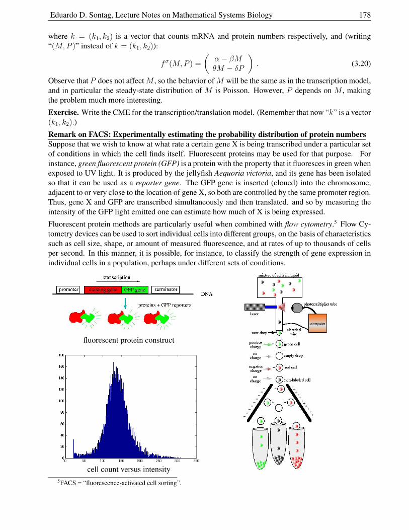
Eduardo D. Sontag, Lecture Notes on Mathematical Systems Biology 178
where k = (k1, k2) is a vector that counts mRNA and protein numbers respectively, and (writing“(M,P )” instead of k = (k1, k2)):
fσ(M,P ) =
(α− βMθM − δP
). (3.20)
Observe that P does not affectM , so the behavior ofM will be the same as in the transcription model,and in particular the steady-state distribution of M is Poisson. However, P depends on M , makingthe problem much more interesting.
Exercise. Write the CME for the transcription/translation model. (Remember that now “k” is a vector(k1, k2).)
Remark on FACS: Experimentally estimating the probability distribution of protein numbersSuppose that we wish to know at what rate a certain gene X is being transcribed under a particular setof conditions in which the cell finds itself. Fluorescent proteins may be used for that purpose. Forinstance, green fluorescent protein (GFP) is a protein with the property that it fluoresces in green whenexposed to UV light. It is produced by the jellyfish Aequoria victoria, and its gene has been isolatedso that it can be used as a reporter gene. The GFP gene is inserted (cloned) into the chromosome,adjacent to or very close to the location of gene X, so both are controlled by the same promoter region.Thus, gene X and GFP are transcribed simultaneously and then translated. and so by measuring theintensity of the GFP light emitted one can estimate how much of X is being expressed.
Fluorescent protein methods are particularly useful when combined with flow cytometry.5 Flow Cy-tometry devices can be used to sort individual cells into different groups, on the basis of characteristicssuch as cell size, shape, or amount of measured fluorescence, and at rates of up to thousands of cellsper second. In this manner, it is possible, for instance, to classify the strength of gene expression inindividual cells in a population, perhaps under different sets of conditions.
fluorescent protein construct
cell count versus intensity5FACS = “fluorescence-activated cell sorting”.
Eduardo D. Sontag, Lecture Notes on Mathematical Systems Biology 179
3.4 Theoretical background, algorithms, and discussion
The abstract theoretical mathematical background for the CME is as follows.
3.4.1 Markov Processes
Suppose that X(t), t ∈ [0,∞) is a stochastic process, that is to say a collection of jointly distributedrandom variables, each of which takes values in a fixed countable set K (K = Zn≥0 in our case).6
From now on, we assume that the process is a continuous-time stationary Markov chain, meaning thatit satisfies the following properties:7
• [Markov] For any two non-negative real numbers t, h, any function x : [0, s] → K, and anyk ∈ K,
P [X(t+ h) = k |X(s) = x(s), 0 ≤ s ≤ t ] = P [X(t+ h) = k |X(t) = x(t) ] .
This property means that X(t) contains all the information necessary in order to estimate thefuture valuesX(T ), T ≥ t: additional values from the past do not help to get a better prediction.
• [Stationarity] The conditional or transition probabilities P [X(s) = ` |X(t) = k ] depend onlyon the difference t− s. This property, also called homogeneity, means that the probabilities donot change over time.
• [Differentiability] With p`k(h) := P [X(t+ h) = ` |X(t) = k ] and pk(t) := P [X(t) = k] forevery `, k ∈ K and all t, h ≥ 0, the functions p`k(h) and pk(t) are differentiable in h, t.
Note the following obvious facts:
•∑
`∈K p`k(h) = 1 for every k ∈ K and h ≥ 0.
• p`k(0) =
0 if ` 6= k1 if ` = k .
Take any t, h > 0, and any ` ∈ K. Then
p`(t+ h) = P [X(t+ h) = `] =∑k∈K
P [X(t+ h) = ` & X(t) = k]
=∑k∈K
P [X(t+ h) = ` |X(t) = k] × P [X(t) = k]
6The more precise notation would be “Xt(ω)”, where ω is an element of the outcome space, but we adopt the standardconvention of not showing ω. We also do not specify the sample space nor the sigma-algebra of measurable sets whichconstitute events to which a probability is assigned. If one imposes the requirement that, with probability one, samplepaths are continuous from the right and have well-defined limits from the left, a suitable sample space can then be takento be a space of piecewise constant mappings from R≥0 to K.
7A subtle fact, usually not mentioned in textbooks, is that conditional probabilities are not always well-defined:“P [A|B] = P [A&B]/P [B]” makes no sense if P [B] = 0. However, for purposes of our discussions, one may de-fine P [A|B] arbitrarily in that case, and no arguments will be affected.
Eduardo D. Sontag, Lecture Notes on Mathematical Systems Biology 180
because the events X(t) = k are mutually exclusive for different k. In other words:
p`(t+ h) =∑k∈K
p`k(h)pk(t) . (3.21)
Similarly. we have8 the Chapman-Kolmogorov equation for the process:
p`˜(t+ h) =∑k∈K
p`k(t) pk˜(h) . (3.22)
3.4.2 The jump time process: how long do we wait until the next reaction?
Suppose thatX(t0) = k, and consider a time interval I = [t0, t0 +h]. IfX(t) 6= k for some t ∈ I , onesays that a “change of state” or an “event” has occurred during the interval, or, for chemical networks,that “a reaction has occurred”.
For each k ∈ K and h ≥ 0, let:
Ck(h) := P [no reaction occurred on [t0, t0 + h] | X(t0) = k]
= P [X(t) = k ∀t ∈ [t0, t0 + h] | X(t0) = k]
(the definition is independent of the particular t0, by homogeneity). The function Ck(h) is non-increasing on h, and Ck(0) = 1. Consider any two h1 ≥ 0 and h2 ≥ 0. We claim that
Ck(h1 + h2) = Ck(h1)Ck(h2) .
Indeed, using the shorthand notation “X(a, b) = k” to mean that “X(t) = k for all t ∈ [a, b]”, wehave:
P [X(t0, t0 + h1 + h2) = k | X(t0) = k]
= P [X(t0, t0 + h1 + h2) = k & X(t0) = k] /P [X(t0) = k]
= P [X(t0, t0 + h1 + h2) = k] /P [X(t0) = k]
= P [X(t0, t0 + h1) = k & X(t0 + h1, t0 + h1 + h2) = k] /P [X(t0) = k]
= P [X(t0, t0 + h1) = k] × P [X(t0 + h1, t0 + h1 + h2) = k | X(t0, t0 + h1) = k] /P [X(t0) = k]
= P [X(t0, t0 + h1) = k] × P [X(t0 + h1, t0 + h1 + h2) = k | X(t0 + h1) = k] /P [X(t0) = k]
= (P [X(t0, t0 + h1) = k] /P [X(t0) = k]) × P [X(t0 + h1, t0 + h1 + h2) = k | X(t0 + h1) = k]
= Ck(h1)Ck(h2)
(we used the formula P [A&B] = P [A] × P [B|A] which comes from the definition of conditionalprobabilities, as well as the Markov property).
Thus, if we define ck(h) = lnCk(h), we have that ck(h1 + h2) = ck(h1) + ck(h2), that is, ck is anadditive function. Notice that the functions Ck, and hence also ck, are monotonic. Therefore each ckis linear: ck(h) = −λkh, for some number λk ≥ 0.9 (The negative sign because ck(h) is the logarithmof a probability, which is a number ≤ 1.) We conclude that Ck(h) = e−λkh.
8Prove this as an exercise.9Read the Wikipedia article on “Cauchy’s functional equation”.
Eduardo D. Sontag, Lecture Notes on Mathematical Systems Biology 181
In summary:P [no reaction takes place on [t0, t0 + h] | X(t0) = k] = e−λkh
from which it follows that
P [at least one reaction takes place on [t0, t0 + h] | X(t0) = k] = 1− e−λkh = λkh+ o(h) .
A central role in both theory and numerical algorithms is played by the following random variable:
Tk := time until the next reaction (“event”) will occur, if the current state isX(t0) = k .
That is,if X(t0) = k, an outcome Tk = h means that the next reaction occurs at time t0 + h.
Observe that, because of the stationary Markov property, Tk depends only on the current state k, andnot on the current time t0,
If the current time is t0, then these two events:
• “the next reaction occurs at some time > h”
• “no reaction occurs during the interval [t0, t0 + h]”
are the same. Thus:P [Tk > h] = e−λkh
which means that:
the variable Tk is exponentially distributed with parameter λk .
Starting from state k, the time to wait until the N th subsequent reaction takes place is:
Tk(1) + Tk(2) + . . .+ Tk(N)
where k(1) = k, k(2) is the state reached after the first reaction, k(3) is the state reached after the secondreaction (starting from state k(2)), and so forth. Note that the choice of which particular “waiting time”random variable T` is used at each step depends on the past state sequence.
If two or more reactions happen during an interval [t0, t0 + h], then Tk(1) + Tk(2) + . . .+ Tk(N) ≤ h forsome N and some sequence of states, so in particular Tk + T` ≤ h for some `. Observe that
P [Tk + T` ≤ h] ≤ P [Tk ≤ h& T` ≤ h] = P [Tk ≤ h]×P [T` ≤ h] = (λkh+o(h))(λ`h+o(h)) = o(h)
because the variables T are conditioned on the initial state, and are therefore independent.10 Theprobability that ≥ 2 reactions happen is upper bounded by
∑` P [Tk + T` ≤ h], where the sum is
taken over all those states ` that can be reached from k after one reaction. We assume from now onthat:
jumps from any given state k can only take place to one of a finite number of possible states `(3.23)
10This step in the argument needs to be made more rigorous: one should specify the joint sample space for the T ’s.
Eduardo D. Sontag, Lecture Notes on Mathematical Systems Biology 182
(as is the case with chemical networks). Thus this sum is finite, and so we can conclude:
P [≥ 2 reactions happen on the interval [t0, t0 + h] | X(t0) = k] = o(h) .
Note that
1− e−λkh = P [some reaction happens on [t0, t0 + h] | X(t0) = k]
= P [exactly one reaction happens on [t0, t0 + h] | X(t0) = k]
+ P [≥ 2 reactions happen on [t0, t0 + h] | X(t0) = k](
= o(h))
and thus
P [exactly one reaction happens on [t0, t0 + h] | X(t0) = k] = 1− e−λkh + o(h) = λkh+ o(h) .
For any two states k 6= `, and any interval [t0, t0 + h], p`k(h) = P [X(t+ h) = ` |X(t) = k ] is thesum of
P [there is a jump from k to ` in the interval [t0, t0 + h]]
plus
P [there is no (direct) jump from k to `, but there is a sequence of jumps that take k into `]
and, as the probability of ≥ 2 jumps is o(h), this last probability is o(h). Thus:
p`k(h) = P [there is a jump from k to ` in the interval [t0, t0 + h]] + o(h) .
Assumption (3.23) then implies that
p`k(h) = o(h) for all but a finite number of states ` .
3.4.3 Propensities
A key role in Markov process theory is played by the infinitesimal transition probabilities defined asfollows:
q`k :=dp`k(h)
dh
∣∣∣∣h=0
Since p`k(h) = o(h) for all but a finite number of states `, it follows that, for each k, there are onlya finite number of nonzero q`k’s. In general, p`k(h) = p`k(0) + q`kh + o(h), so, since p`k(0) = 0 if` 6= k and = 1 if ` = k:
p`k(h) =
hq`k + o(h) if ` 6= k1 + hqkk + o(h) if ` = k.
Recall that λk is the parameter for the exponentially distributed random variable Tk that gives the timeof the next reaction provided that the present state is k. We claim that:
qkk = −λk for all k .
Indeed, pkk(h) := P [X(t+ h) = k |X(t) = k ], and this event is the union of the mutually exclusiveevents “no reaction happened” (which has probability e−λkh) and “two or more reactions happened,
Eduardo D. Sontag, Lecture Notes on Mathematical Systems Biology 183
and the end state is again k”. This second event has probability o(h), because the probability thatmore than one reaction happens (even if the final state is different) is already o(h). Thus: pkk(h) =e−λkh + o(h), which gives (dpkk/dt)(0) = −λk, as claimed.
Note also that, since∑
`∈K p`k(h) = 1 for all h, taking d/dh|h=0 gives:∑`∈K
q`k = 0 or, equivalently, qkk = −∑` 6=k
q`k (3.24)
and hence also λk =∑6=k q`k, for every k.
Recall that the Chapman-Kolmogorov equation (3.22) says that p`˜(t+ h) =∑
k∈K p`k(t) pk˜(h) forall t, h. By definition, q`k = (dp`k/dh)(0), so taking the derivative with respect to h and evaluating ath = 0, we arrive at the forward Kolmogorov differential equation
dp`˜dt
=∑k∈K
p`k qk˜ (3.25)
which is an equation relating conditional probabilities through the infinitesimal transitions. Similarly,the corresponding equation on probabilities (3.21) is pk(t + h) =
∑`∈K pk`(h)p`(t), which leads
under differentiation to:dpkdt
=∑`∈K
qk` p` . (3.26)
This differential equation is often also called the forward Kolmogorov equation, and it is exactly thesame as the CME (3.3) dpk
dt=∑m
j=1 ρσj (k − γj) pk−γj −
∑mj=1 ρ
σj (k) pk, where
the propensities ρσj (k) are, by definition, the infinitesimal transition probabilities q`k.
More precisely, consider the m reactions Rj , which produce the stoichiometry changes k 7→ k + γjrespectively. We define ρσj (k) = q`k for ` = k + γj , j = 1, . . . ,m. So:
qk` =
ρσj (`) if ` = k − γj for some j ∈ 1, . . . ,m−∑6=k q`k = −
∑mj=1 ρ
σj (k) if ` = k (recall (3.24))
0 otherwise .
Since λk = −qkk,
λk =∑`6=k
q`k =m∑j=1
ρσj (k) . (3.27)
3.4.4 Interpretation of the Master Equation and propensity functions
Since, by definition of the q`k’s, pk+γj ,k(h) = qk+γj ,kh + o(h) = ρσj (k)h + o(h) and pkk(h) =1 + qkkh+ o(h) = 1−
∑mj=1 ρ
σj (k)h+ o(h),
P [X(t+ h) = k + γj |X(t) = k] = ρσj (k)h + o(h) ≈ ρσj (k)h
and
P [X(t+ h) = k |X(t) = k] = 1−m∑j=1
ρσj (k)h + o(h) ≈ 1−m∑j=1
ρσj (k)h .
Eduardo D. Sontag, Lecture Notes on Mathematical Systems Biology 184
Since the probability that more than one reaction occurs on an interval of length h is o(h), the proba-bility that X(t+ h) = k + γj is approximately the same as that ofRj happening in the interval. Thisjustifies the intepretation of the propensity of the reactionRj as:
ρσj (k)h ≈ probability that the reactionRj will take place, during a time interval [t, t+h]of (short) duration h, if the state was k at time t.
In other words, ρσj is the rate at which the reaction Rj “fires”. This rate depends, obviously, on howmany units of the various reactants are present (k). Furthermore, with this interpretation,
ρσj (k)h pk(t) ≈P [reactionRj takes place during interval [t, t+ h] | state was k at time t]× P [state was k at time t]= P [state was k at time t & reactionRj takes place during interval [t, t+ h]] ,
and som∑j=1
ρσj (k)h pk(t)
is the probability that the state at time t is k and some reaction takes place during the time interval[t, t + h]. (Implicitly assuming that these events are mutually exclusive, i.e. at most one reaction canhappen, if the time interval is very short.)
Therefore, the second term in (3.4):(1−
m∑j=1
ρσj (k)h
)pk(t) = pk(t)−
m∑j=1
ρσj (k)h pk(t)
≈ P [initial state was k \ initial state was k and some reaction happens during interval [t, t+ h]]= P [initial state was k and no reaction happens during interval [t, t+ h]]
= P [final state is k and no reaction happens during interval [t, t+ h]]
where the last equality is true because the events:no reaction happened and the initial state was k
andno reaction happened and the final state is k
are the same.
On the other hand, regarding the m first terms in (3.4), note that the event:reactionRj happened and the final state is k
is the same as the event:reactionRj happened and the initial state was k − γj ,
and the probability of this last event is ≈ ρσj (k − γj)h pk−γj(t)In summary, we are justified in interpreting (3.4) as asserting that the probability of being in state k atthe end of the interval [t, t+ h] is the sum of the probabilities of the following m+ 1 events:
• for each possible reactionRj , the reactionRj happened, and the final state is k, and
• no reaction happened, and the final state is k.
Eduardo D. Sontag, Lecture Notes on Mathematical Systems Biology 185
3.4.5 The embedded jump chain
The exponentially distributed variable T tells what is the waiting time until the next reaction. In orderto understand the behavior of the system as a sequence of jumps, one needs, in addition, a randomvariable that specifies which reaction takes place next (or, more generally for Markov processes, towhich state is the next transition), given that a transition happens.
For each ` 6= k and h, let α`k(h) be the probability that the state is ` at time t + h, assuming thatthe initial state is k and that some reaction has happened. If k is not an absorbing state, that is, iftransitions out of k are possible, an elementary calculation with conditional probabilities (using thatX(t+ h) = ` implies X(t+ h) 6= k) shows that:11
α`k(h) = P [X(t+ h) = ` | X(t) = k & X(t+ h) 6= k] =P [X(t+ h) = ` |X(t) = k]
P [X(t+ h) 6= k |X(t) = k].
Ideally, one would like to compute this expression, but the transition probabilities are hard to obtain.However,
limh→0
α`k(h) = limh→0
p`k(h)
1− pkk(h)= lim
h→0
hq`k + o(h)
1− (1 + hqkk + o(h))= − q`k
qkk=
q`k∑˜6=k q˜k =: d(k)` .
(If k is an absorbing state, the denominators are zero, but in that case we know that α`k(h) = 0 for all` 6= k.)
Although in principle only an approximation, it was proved by J.L. Doob12 that the discrete probabilitydistribution d(k)
` (for any fixed k, over all ` 6= k), together with the process Tk, characterize a processwith the same probability distribution as the original X(t). By itself, the matrix D with entries d(k)
`
is the transition matrix for the discrete-time embedded Markov chain or jump chain of the process.This discrete chain provides a complete statistical description of the possible sequences of statesvisited, except that it ignores the actual times at which jumps occur. It is very helpful in theoreticaldevelopments, especially in the classification of states (“recurrent”, “transient”, etc.) of the continuousprocess.
3.4.6 The stochastic simulation algorithm (SSA)
To understand the behavior of the process X(t), one could attempt to solve the CME (with a knowninitial p(0)) and compute the probability vector p(t). For most problems, this is a computationallyvery difficult task, starting with the fact that p(t) is an infinite vector. Thus, it is often useful tosimulate sample paths of the process. Statistics, such as means and variances, can then be obtainedby averaging the results of several such simulations.
The naıve approach to simulation is to discretize time into small intervals, and iterate on intervals,randomly deciding at each instant whether a reaction happens. This is not at all an efficient way toproceed: if the discretization is too fine, no reactions will take place in most intervals, and the iterationstep is wasted; if the discretization is too gross, we miss fast behaviors. Luckily, there is a far betterway to proceed. The basic method13 for simulating sample paths of CME’s is the stochastic simulation
11The calculation is: P [A|B&C] = P [A&B&C]P [B&C] = P [A&B]
P [B&C] == P [A|B]P [B]P [C|B]P [B] = P [A|B]
P [C|B] .12“Markoff chains - Denumerable case,” Transactions of the American Mathematical Society 58(1945): 455-473.13There are many variants that are often more efficient to implement, but the basic idea is always the same.
Eduardo D. Sontag, Lecture Notes on Mathematical Systems Biology 186
algorithm. Also known as the kinetic Monte Carlo algorithm14, it has been probably known and usedfor a long time, at least since J.L. Doob’s work cited earlier, but in its present form was introducedindependently by A.B. Bortz, M.H. Kalos, and J.L. Lebowitz15 and by D.T. Gillespie16 (the SSA isoften called the “Gillespie algorithm” in the systems biology field).
The method is very simple: if the present state is k, first use the random variable Tk to compute thenext-reaction time, and then pick the particular reaction according to the discrete distribution d(k)
j ,where we are writing d(k)
j instead of d(k)k+γj
, for each j ∈ 1, . . . ,m (all other d(k)` = 0). With the
notations for propensities used in the CME, we have, for each J ∈ 1, . . . ,m:
d(k)J =
qk+γJ ,k∑˜=k+γjq˜,k =
ρσJ(k)∑mj=1 ρ
σj (k)
=ρσJ(k)
λk.
Generating samples of the exponential random variable Tk is easy provided that a uniform (pseudo)random number generator is available, like the “rand” function in MATLAB. In general, if U is auniformly distributed random variable on [0, 1], that is, P [U < p] = p for p ∈ [0, 1], then T = − lnU
λ
is an exponentially distributed random variable with parameter λ, because:
P [T > t] = P[− lnU
λ> t
]= P
[U < e−λt
]= e−λt .
Here is the pseudo-code for the SSA:
Initialization:
1. inputs: state k, maximal simulation time Tmax
2. set current simulation time t := 0.
Iteration:
1. compute ρσj (k), for each reaction Rj, j = 1, . . . ,m
2. compute λ :=∑m
j=1 ρσj (k)
3. if λ = 0, stop (state is an absorbing state, no further transitionsare possible)
4. generate two uniform random numbers r1, r2 in [0, 1]
5. compute T := − 1λ
ln r1
6. if t+ T > Tmax, stop
7. find the index J such that 1λ
∑J−1j=1 ρ
σj (k) ≤ r2 <
1λ
∑Jj=1 ρ
σj (k)
8. update k := k + γJ
9. update t := t+ T.
Note that, in step 7, the probability that a particular j = J is picked is the same as the length of theinterval [ 1
λ
∑J−1j=1 ρ
σj (k), 1
λ
∑Jj=1 ρ
σj (k)], which is 1
λρσJ(k) = d
(k)J .
14In general, “Monte Carlo” methods are algorithms that rely on repeated random sampling to compute their results.15“New algorithm for Monte-Carlo simulations of Ising spin systems,” J. Comput. Phys. 17(1975): 10-18.16“A general method for numerically simulating the stochastic time evolution of coupled chemical reactions,” Journal
of Computational Physics 22(1976): 403-434.
Eduardo D. Sontag, Lecture Notes on Mathematical Systems Biology 187
Of course, one will also want to add code to store the sequence of states k and the jump times T , soas to plot sample paths. Note that, in MATLAB, if v is an array with the numbers ρσj (k), then thecommand “J = find(cumsum(v)>sum(r2 ∗ v))” provides the index J .
Exercise. (1) Implement the SSA in your favorite programming system (MATLAB, Maple, Math-ematica). (2) Take the mRNA/protein model described earlier, pick some parameters, and an initialstate; now plot many sample paths, averaging to get means and variances as a function of time, aswell as steady state means and variances. (3) Compare the latter with the numbers obtained by usingtheory as described later. 2
Remark: An equivalent way to generate the next reaction in the SSA (“direct method”) is as fol-lows (the “first reaction method”, also discussed by Gillespie): generate m independent exponentialrandom variables Tj , j = 1, . . . ,m, with parameters λ(j)
k = ρσj (k) respectively –we think of Tj asindicating when the reaction j would next take place– and pick the “winner” (smallest Tj) as thetime (and index) of the next reaction. The same result obtains, because of the following generalmathematical fact:17 if T1, . . . , Tm are independent exponentially distributed random variables withrate parameters µ1, . . . , µm respectively, then T = minj Tj is also exponentially distributed, withparameter µ =
∑j µj . This fact is simple to prove:
P [T > t] = P [T1 > t& . . . & Tm > tm] =∏j
P [Tj > t] =∏j
e−µjt = e−µt .
Moreover, it is also true that the index J of the variable which achieves the minimum –i.e., the“next reaction”– is a discrete random variable with is distributed according to the law P [J = p] =µp/(
∑j µj).
From a computational point of view, the first reaction method would appear to be less efficient than thedirect method, as m random variables have to be generated at each step (compared to just two for thedirect method). However, the first reaction method has one advantage: since any given reaction willtypically affect only a small number of species, there is no need to re-compute propensities for thoseindices j for which ρσj (k) has not changed. This observation, together with the use of an indexedpriority queue data structure, and a re-use of previously-generated Tj’s, leads to a more efficientalgorithm, the “next reaction method” due to M.A. Gibson and J. Bruck.18
3.4.7 Interpretation of mass-action kinetics
We explain now, through an informal discussion, how the formula (3.5): ρσj,Ω(k) =cj
ΩAj−1
(kaj
)(j =
1, . . . ,m) is derived.
Suppose that the state of the system at time t is k = (k1, . . . , kn)′, and we consider an interval oflength 0 < h 1. What is the probability of a reactionRj taking place in the interval [t, t+ h]?
For this reaction to even have a chance of happening, the first requirement is that some subset Sconsisting ofa1,j units of species S1, a2,j units of species S2, a3,j units of species S3, . . . , an,j units of species Sn
17While formally this provides the same numbers, it is not clear a priori why reaction times should be independent!18“Efficient exact stochastic simulation of chemical systems with many species and many channels,” J. Phys. Chem. A
104(2000): 1876-1889.
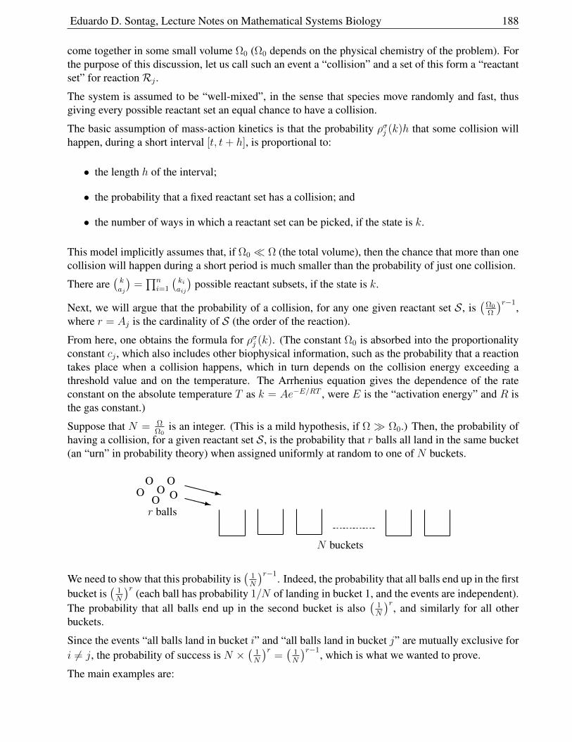
Eduardo D. Sontag, Lecture Notes on Mathematical Systems Biology 188
come together in some small volume Ω0 (Ω0 depends on the physical chemistry of the problem). Forthe purpose of this discussion, let us call such an event a “collision” and a set of this form a “reactantset” for reactionRj .
The system is assumed to be “well-mixed”, in the sense that species move randomly and fast, thusgiving every possible reactant set an equal chance to have a collision.
The basic assumption of mass-action kinetics is that the probability ρσj (k)h that some collision willhappen, during a short interval [t, t+ h], is proportional to:
• the length h of the interval;
• the probability that a fixed reactant set has a collision; and
• the number of ways in which a reactant set can be picked, if the state is k.
This model implicitly assumes that, if Ω0 Ω (the total volume), then the chance that more than onecollision will happen during a short period is much smaller than the probability of just one collision.
There are(kaj
)=∏n
i=1
(kiaij
)possible reactant subsets, if the state is k.
Next, we will argue that the probability of a collision, for any one given reactant set S, is(
Ω0
Ω
)r−1,where r = Aj is the cardinality of S (the order of the reaction).
From here, one obtains the formula for ρσj (k). (The constant Ω0 is absorbed into the proportionalityconstant cj , which also includes other biophysical information, such as the probability that a reactiontakes place when a collision happens, which in turn depends on the collision energy exceeding athreshold value and on the temperature. The Arrhenius equation gives the dependence of the rateconstant on the absolute temperature T as k = Ae−E/RT , were E is the “activation energy” and R isthe gas constant.)
Suppose that N = ΩΩ0
is an integer. (This is a mild hypothesis, if Ω Ω0.) Then, the probability ofhaving a collision, for a given reactant set S, is the probability that r balls all land in the same bucket(an “urn” in probability theory) when assigned uniformly at random to one of N buckets.
XXXXzXXXz
OO
OO
OO
r balls
N buckets
We need to show that this probability is(
1N
)r−1. Indeed, the probability that all balls end up in the firstbucket is
(1N
)r (each ball has probability 1/N of landing in bucket 1, and the events are independent).The probability that all balls end up in the second bucket is also
(1N
)r, and similarly for all otherbuckets.
Since the events “all balls land in bucket i” and “all balls land in bucket j” are mutually exclusive fori 6= j, the probability of success is N ×
(1N
)r=(
1N
)r−1, which is what we wanted to prove.
The main examples are:
Eduardo D. Sontag, Lecture Notes on Mathematical Systems Biology 189
(0) zeroth-order reactions, in which an isolated species is created by means of a process which involveprecursors which are not explicitly made a part of the model and which are well-distributed in space;in this case Aj = 0 and ρσj (k) is independent of k, so it is just a constant, proportional to the volume;
(1) first-order or monomolecular reactions, in which a single unit of species i is degraded, diluted,decays, flows out, or gets transformed into one or more species; in this case Aj = 1 and exactly oneaij is equal to 1 and the rest are zero, so ρσj (k) = cjki (since Ω0 = 1);
(2) homogeneous second-order (bimolecular) reactions involving two different species Si and S`,one unit of each; now there two entries aij and a`j equal to 1, and the rest are zero, Aj = 2, andρσj (k) = 1
Ωcjkik`;
(3) homogeneous second-order (bimolecular) reactions involving two units of the same species Si;now Aj = 2 and exactly one aij is equal to 2 and the rest are zero, so ρσj (k) = 1
Ωcjki(ki−1)
2.
It is frequently argued that at most mono and bimolecular reactions are possible in the real world, sincethe chance of three or more molecules coming together in a small volume is vanishingly small. Inthis case, reactions involving multiple species would really consist of a sequence of more elementarybimolecular reactions, involving short-lived, intermediate, species. However, multi-species reactionsmight still make sense, either as an approximation of a more complicated sequence that occurs veryfast, or if molecules are very large compared to the volume, of if the model is one that involvesnon-chemical substances (for example, in population biology).
Eduardo D. Sontag, Lecture Notes on Mathematical Systems Biology 190
3.5 Moment equations and fluctuation-dissipation formula
We next see how to obtain equations for the derivatives of the mean E [Xi(t)] and the covarianceVar [X(t)] of X(t), assuming that the probability density of X(t) is given by a CME as in (3.3). Nospecial form needs to be assumed for the propensities, for these theoretical considerations to be valid,but in examples we use mass-action kinetics.
We provide first a very general computation, which we will later specialize to first and second mo-ments. Suppose for this purpose that we have been given a function M which will be, in our twoexamples, a vector- of matrix-valued function defined on the set of non-negative integers. More ab-stractly, we take M : Zn≥0 → V , where V is any vector space. For first moments (means), we haveV = Rn and M(k) = k. For second moments, V = Rn×n, the space of all n × n matrices, andM(k) = kk′.19
The first goal is to find a useful expression for the time derivative of E [M(X(t))]. The definition ofexpectation gives:20
E [M(X(t))] =∑k∈Zn≥0
pk(t)M(k)
because P [X(t) = k] = pk(t). We have:
d
dtE [M(X(t))] =
∑k∈Zn≥0
dpkdt
(t)M(k) =∑k∈Zn≥0
(m∑j=1
ρσj (k − γj) pk−γj −m∑j=1
ρσj (k) pk
)M(k) .
Note this equality, for each fixed j:∑k∈Zn≥0
pk−γj(t)ρσj (k − γj)M(k) =
∑k∈Zn≥0
pk(t)ρσj (k)M(k + γj)
(by definition, ρσj (k − γj) = 0 unless k ≥ γj , so one may perform a change of variables k = k − γj).There results:
d
dtE [M(X(t))] =
∑k,j
pk(t)ρσj (k)M(k + γj) −
∑k,j
pk(t)ρσj (k)M(k)
=∑k∈Zn≥0
pk(t)m∑j=1
ρσj (k) [M(k + γj)−M(k)] .
Let us define, for any γ ∈ Zn≥0, the new function ∆γM given by (∆γM)(k) := M(k + γ) −M(k).With these notations,
d
dtE [M(X(t))] = E
[m∑j=1
ρσj (X(t)) ∆γM(X(t))
]. (3.28)
Note that this is not an ordinary differential equation for E [M(X(t)], because the right-hand side isnot, generally, a function of E [M(X(t))]. In some cases, however, various approximations result indifferential equations, as discussed below.
19As usual, prime indicates transpose, so this is the product of a column vector by a row vector, which is a rank 1 matrixif k 6= 0.
20Note that this is a deterministic function, not depending on the random outcomes of the process.
Eduardo D. Sontag, Lecture Notes on Mathematical Systems Biology 191
Remark. Suppose that M is a polynomial of degree δM and that the propensities are polynomials ofdegree ≤ δρ (the maximal order of reactions, in the mass action case). Then ∆γM is a polynomial ofdegree δM − 1, so the monomials appearing inside the expectation have degree ≤ δρ + δM − 1. Thismeans that d
dtE [M(X(t))] depends on moments of order ≤ δρ + δM − 1. Thus, if all reactions have
order at most 1, a system of differential equations can obtained for the set of moments of up to anyfixed order: the derivative of each moment depends only on equal and lower-order ones, not highermoments. On the other hand, if some reactions have order larger than 1, then δρ + δM − 1 > δM , soin general no clsoed set of equations is available for any finite subset of moments.
3.5.1 Means
For the mean E [X(t)], we have M(k) = k, so ∆jM(k) = k+ γj − k = γj (a constant function), andthus:
m∑j=1
ρσj (X(t)) ∆γM(X(t)) =m∑j=1
ρσj (X(t)) γj = fσ(X(t))
where, recall, we defined the n-column vector:
fσ(k) :=m∑j=1
ρσj (k) γj k ∈ Zn≥0 .
With these notations, Equation (3.28) specializes to:
d
dtE [X(t)] = E [fσ(X(t))] . (3.29)
Recall that fσ(k) can also be written in the form
fσ(k) = ΓRσ(k) (3.30)
where Rσ(k) = (ρσ1 (k), . . . , ρσm(k))′ and Γ is the stoichiometry matrix.
For mass-action kinetics, the function fσ is basically the same one21 that is used in the deterministicdifferential equation model for the corresponding chemical network. Thus, it is a common mistaketo think that the deterministic equation represents an equation that is satisfied by the mean µ(t) =E [X(t)], that is to say, to believe that dµ/dt = fσ(µ). However, the precise formula is (3.29).Since expectation of a nonlinear function is generally not the same as the nonlinear function of theexpectation22, (3.29) is, in general, very different from (d/dt)E [X(t)] = fσ(E [X(t)]). One importantexception, which permits the replacement E [fσ(X(t))] = fσ(E [X(t)]), is that in which fσ is anaffine function (linear + constant), that is to say if all propensities are affine, which for mass-actionkinetics means that all the reactions involve zero or at most one reactant:
d
dtE [X(t)] = fσ(E [X(t)]) if all reactions are mass-action of order 0 or 1 . (3.31)
21There is just a very minor difference, discussed later, having to do with replacing terms such as “x(x − 1)” in asecond-order homodimerization reaction by the simpler expression x2.
22Example: E[X2]6= E [X]
2; in fact, the variance of X is precisely the concept introduced in order to quantify thedifference between these two quantities!
Eduardo D. Sontag, Lecture Notes on Mathematical Systems Biology 192
On the other hand, even for reactions of arbitrary order, one might expect that Equation (3.31) holds atleast approximately provided that the variance of X(t) is small, so that X(t) is almost deterministic.More precisely, one has the following argument.
Let us assume that the function fσ, which is defined only for non-negative integer vectors, can beextended to a differentiable function, also written as fσ(x), that is defined for all non-negative realnumbers x. This is the case with all propensities that are used in practice, such as those arising frommass-action kinetics. Thus, around each vector ξ, we may expand fσ(x) to first-order around x = ξ:
fσ(x) = fσ(ξ) + J(ξ)(x− ξ) + gξ(x− ξ) (3.32)
where J(x) is the Jacobian matrix of fσ evaluated at x = ξ and where gξ is a vector function which iso(|x− ξ|). When f is second-order differentiable, the entries giξ of the vector gξ can be expressed as:
giξ(x) =1
2(x− ξ)′Hi(ξ) (x− ξ) + o(|x− ξ|2)
where Hi(ξ) is the Hessian of the ith component of the vector field fσ (the matrix of second orderpartial derivatives) evaluated at x = ξ.
For notational simplicity, let us write µ for means: µ(t) = E [X(t)]. In the particular case thatξ = µ(t) and x = X(t) (along a sample path), we have:
fσ(X(t)) = fσ(µ(t)) + J(µ(t)) (X(t)− µ(t)) + gµ(t)(X(t)− µ(t)) . (3.33)
Now, J(µ(t)) is a deterministic function, so, since the expectation operator is linear,
E [J(µ(t)) (X(t)− µ(t))] = J(µ(t)) (E [X(t)]− µ(t)) = J(µ(t)) (E [X(t)]− E [X(t)]) = 0 .
Since also fσ(µ(t)) is deterministic, it follows that:
d
dtE [X(t)] = E [fσ(X(t))] = fσ(E [X(t)]) + G(t)
whereG(t) = E
[gµ(t)(X(t)− µ(t))
]. (3.34)
This term involves central moments (covariances, etc.) of order ≥ 2.
3.5.2 Variances
For the matrix of second order moments E [X(t)X(t)′], we have M(k) = kk′, so
∆jM(k) = (k + γj)(k + γj)′ − kk′ = kγ′j + γjk
′ + γjγ′j
and so Equation (3.28) ddtE [M(X(t))] = E
[∑mj=1 ρ
σj (X(t)) ∆γM(X(t))
]specializes to:
d
dtE [X(t)X(t)′] = E
[m∑j=1
ρσj (X(t))X(t) γ′j
]+E
[m∑j=1
ρσj (X(t)) γj X(t)′
]+
m∑j=1
E[ρσj (X(t))
]γjγ
′j
(3.35)
Eduardo D. Sontag, Lecture Notes on Mathematical Systems Biology 193
(note that the ρσj (X(t))’s are scalar, and that X(t) and the γj’s are vectors). Since we had definedfσ(k) =
∑mj=1 ρ
σj (k) γj , the second term in this sum can be written as E [fσ(X(t))X(t)′]. Similarly,
the first term is E [X(t) fσ(X(t))′]. The last term can be written in the following useful form.
We introduce the n× n diffusion matrix23 B(k) = (Bpq(k)) which has the following entries:
Bpq(k) =m∑j=1
ρσj (k) γpj γqj , p, q = 1, . . . , n , (3.36)
where γpj is the pth row of the column vector γj , that is to say the (p, j)th entry of the stoichiometrymatrix Γ, so that γpjγqj is the (p, q)th entry of the matrix γjγ′j . Note that B is an n × n symmetricmatrix. In summary, we can write (3.35) as follows:
d
dtE [X(t)X(t)′] = E [X(t) fσ(X(t))′] + E [fσ(X(t))X(t)′] + E [B(X(t))] . (3.37)
One interpretation of the entries E[Bpq(X(t)
]is as follows. The product γpjγqj is positive provided
both species Sp and Sq change with the same sign (both increase or both decrease) when the reactionRj fires. The product is negative if one species increases but the other decreases, whenRj fires. Theabsolute value of this product is large if at least one of these two species jumps by a large amount.Finally, the expected value of the coefficient ρσj (k) quantifies the rate at which the correspondingreaction takes place. In this manner, E
[Bpq(X(t)
]contributes toward an instantaneous change in the
correlation between species Sp and Sq.
An equation for the derivative of the variance is easily obtained from here. By definition, Var [X(t)] =E [X(t)X(t)′]−E [X(t)]E [X(t)]′, so we need to compute the derivative of this last term. For a vectorfunction v = v(t), (d/dt)vv′ = v(dv/dt)′ + (dv/dt)v′, so with dv/dt = d
dtE [X(t)] = E [fσ(X(t))]
from (3.29),
d
dtVar [X(t)] = E [(X(t)− µ(t)) fσ(X(t))′] + E [fσ(X(t)) (X(t)− µ(t))′] + E [B(X(t))]
(3.38)where we wrote µ(t) = E [X(t)] for clarity.
Exercise. Show that an alternative way of writing the third term in the right-hand side of (3.38) is asfollows:
Γ diag (E [ρσ1 (X(t))] , . . . ,E [ρσm(X(t))]) Γ′ (3.39)
(where “diag (r1, . . . , rm)” means a diagonal matrix with entries ri in the diagonal). 2
The first-order Taylor expansion of fσ, fσ(X(t)) = fσ(µ(t)) + J(µ(t))(X(t)−µ(t)) + gµ(t)(X(t)−µ(t)), given in (3.33), can be substituted into the term E [fσ(X(t)) (X(t)− µ(t))′] in the formula (3.38)for the covariance, giving (dropping the arguments “t” for readability):
E [fσ(X)(X − µ)′] = E [fσ(µ)(X − µ)′] + E [J(µ)(X − µ)(X − µ)′] + E [gµ(X − µ)(X − µ)′]
= J(µ)Var [X] + E [gµ(X − µ)(X − µ)′]
23Normally, “diffusion” is interpreted in a spatial sense. Here it is thought of, instead, as diffusion in “concentrationspace”.
Eduardo D. Sontag, Lecture Notes on Mathematical Systems Biology 194
where we used that fσ(µ(t)) and J(µ(t)) are deterministic and that E [X − µ] = 0. Similarly,
E [(X − µ)fσ(X)′] = Var [X] J(µ)′ + E [(X − µ) gµ(X − µ)′]
(the covariance matrix is symmetric, so there is no need to transpose it). Therefore,
d
dtVar [X(t)] = Var [X(t)] J(µ(t))′ + J(µ(t))Var [X(t)] + E [B(X(t))] + α(t) (3.40)
where α(t) = E[(X(t)− µ(t)) gµ(t)(X(t)− µ(t))′ + (X(t)− µ(t)) gµ(t)(X(t)− µ(t))′
]. Dropping
the term α(t), one has the fluctuation-dissipation formula:
d
dtVar [X(t)] ≈ Var [X(t)] J(µ(t))′ + J(µ(t))Var [X(t)] + E [B(X(t))] (FD) . (3.41)
If the higher-order moments of X(t) are small, one may be justified in making this approximation,because α(t) is o(|X(t)− µ(t)|2), while the norm of the covariance matrix is O(|X(t)− µ(t)|2).
Equation (3.41) is sometimes called the mass fluctuation kinetics equation, and the term “fluctuation-dissipation” is used for a slightly different object, as follows. Suppose that we expandB(x) as a Taylorseries around the mean E [X(t)]. Arguing as earlier, we have that E [B(X(t))] = B(E [X(t)]) +o(|X(t)− µ(t)|). This suggests replacing the last term in (FD) by B(E [X(t)]).
3.5.3 Reactions or order ≤ 1 or ≤ 2
The special case in which fσ is a polynomial of degree two is arguably the most general that oftenneeds to be considered. (Recall the discussion about reactions of order > 2.) In this case, the func-tion gξ in (3.32) is a vector field that is quadratic on the coordinates of X(t) − µ(t), with constantcoefficients, because the Hessian of a quadratic polynomial is constant. The expectations of suchexpressions are the covariances Cov [Xi(t), Xj(t)] (variances if i = j). So, G(t) is a linear functionL of the n2 entries of Var [X(t)]. The linear function L can be easily computed from the secondderivatives of the components of fσ. Similarly, as the entries of the diffusion matrix (3.36) are poly-nomials of degree equal to the largest order of the reactions, when all reactions have order ≤ 2 theterm E [B(X(t))] is an affine linear function of the entries of E [X(t)] and Var [X(t)], which we writeas H0 +H1E [X(t)] +H2Var [X(t)]. Thus:
For mass-action kinetics and all reactions of order at most 2, the fluctuation-dissipation equationsays that the mean µ(t) = E [X(t)] and covariance matrix Σ(t) = Var [X(t)] satisfy
µ = fσ(µ) + LΣ (3.42a)Σ ≈ Σ J(µ)′ + J(µ) Σ + H0 +H1µ+H2Σ (3.42b)
(where the “approximate” sign indicates that α, which involves third-order moments, because gµ(t) isquadratic, was dropped). Moreover, the function J(µ(t)) is linear in µ(t).
The FD formula is exact for zero- and first-order mass-action reactions, because in that case theHessian and thus gµ(t) are zero, so also α(t) ≡ 0. Moreover, in this last case the entries Bpq(k) =∑m
j=1 ρσj (k)γpjγqj of the diffusion matrix are also affine, so that the last term is just B(E [X(t)]). It is
worth emphasizing this fact:
Eduardo D. Sontag, Lecture Notes on Mathematical Systems Biology 195
For mass-action kinetics and all reactions of order zero or one, the mean µ(t) = E [X(t)] andcovariance matrix Σ(t) = Var [X(t)] are solutions of the coupled system of differential equations
µ = fσ(µ) (3.43a)Σ = Σ J ′ + J Σ + B(µ) (3.43b)
and in this case J does not depend on µ, because J is a constant matrix, being the Jacobian of anaffine vector field. Also,
B(µ) = Γ diag (ρσ1 (µ), . . . , ρσm(µ)) Γ′ (3.44)
in the case of order ≤ 1.
Note that (3.43) is a set of n + n2 linear differential equations. Since covariances are symmetric,however, one can equally well restrict to the equations on the diagonal and upper-triangular part of Σ,so that it is sufficient to solve n+ n(n+ 1)/2 equations.
The term “fluctuation-dissipation” is used because the first two terms for Σ may be though of asdescribing a “dissipation” of initial uncertainty, while the last term can be thought of as a “fluctuation”due to future randomness. To understand the dissipation component, let’s discuss what would happenif the fluctuation term were not there. Then (FD) is a linear differential equation on Var [X(t)] (a“Lyapunov equation” in control theory). Given the initial variance Var [X(0)], a solution can becomputed. This solution is identically zero when X(0) is perfectly known (that is, p(0) has exactlyone nonzero entry), because Var [X(0)] = 0 in that case. But even for nonzero Var [X(0)], and underappropriate stability conditions one would have that Var [X(t)] → 0 as t → ∞. If a matrix J haseigenvalues with negative real part, then the operator P 7→ PJ ′ + JP on symmetric matrices has alleigenvalues also with negative real part.24 So if µ(t) is approximately constant and the linearizationof the differential equation for the mean is stable, the equation for the variance will be, too. Since ingeneral the matrices J(µ(t)) depend on t, this argument is not quite correct, but it provides the basicintuition for the term “dissipation”.
24This is because the eigenvalues of this operator are the sums of pairs of eigenvalues of J ; see e.g. the author’s controltheory textbook.
Eduardo D. Sontag, Lecture Notes on Mathematical Systems Biology 196
3.6 Generating functions
We next discuss how to use generating functions in order to (1) find solutions of the CME, or atleast (2) find differential equations satisfied by moments. Often only simple problems can be solvedexplicitly with this technique, but it is nonetheless a good source of theoretical insight.
We assume that p(t), an infinite vector function of time indexed by k ∈ K = Zn≥0, is a solution of theCME (3.3):
dpkdt
=m∑j=1
ρσj (k − γj) pk−γj −m∑j=1
ρσj (k) pk .
The (probability) generating function P (z, t) is a scalar-valued function of time t ≥ 0 and of nauxilliary variables z = (z1, . . . , zn) (which may be thought of as complex variables), defined asfollows:
P (z, t) := E[zX]
=∑k∈K
pk(t) zk (3.45)
where we denote zk := zk11 . . . zknn and z0i = 1. As the pk(t)’s are non-negative and add up to one, the
series is convergent for z = 1 (we write the vector (1, . . . , 1) as “1” when clear from the context):
P (1, t) = 1 for all t ≥ 0. (3.46)
Moments of arbitrary order can be computed once that P is known. For example,
∂P (z, t)
∂z
∣∣∣∣z=1
= E [X(t)] ,
where we interpret the above partial derivative as the vector(∂P (t,z)∂z1
∣∣∣z=1
, . . . , ∂P (t,z)∂zm
∣∣∣z=1
)′. Also,
∂2P (z, t)
∂zi∂zj
∣∣∣∣z=1
=
E [Xi(t)Xi(t)] if i 6= jE [Xi(t)
2]− E [Xi(t)] if i = j .
Note that Var [X(t)] can be computed from these formulas.
Exercise. Prove the above two formulas. 2
We remark that there are other power series than are often associated to P , especially the momentgenerating function25
M(θ, t) := E[eθX]
=∑k∈K
pk(t) eθk
where we define eq = eq1 . . . eqn .
Of course, actually computing P (z, t) from its definition is not particularly interesting, since thewhole purpose of using generating functions is to gain information about the unknown pk(t)’s. Theidea, instead, is to use the knowledge that p(t) satisfies an infinite system of ordinary differentialequations in order to obtain a finite set of partial differential equations for P . Sometimes these PDE’scan be solved, and other times just the form of the PDE will be enough to allow computing ODE’s formoments. We illustrate both of these ideas next, through examples.
25The terminology arises from the fact that the coefficients of the Taylor expansions of P and M , at z = 0 and θ = 0,give the probabilities and moments, respectively.
Eduardo D. Sontag, Lecture Notes on Mathematical Systems Biology 197
Let us start with the mRNA example given by the reactions in (3.6), 0α−→M β−→0, for which (cf. (3.7)-
(3.9)) G = (1,−1), ρσ1 (k) = α, ρσ2 (k) = βk, fσ(k) = α− βk, and the CME is
dpkdt
= αpk−1 + (k + 1)βpk+1 − αpk − kβpk .
Let us compute now a PDE for P (z, t). For simplicity, from now on we will write ∂∂tP as Pt and ∂
∂zP
as Pz.
By definition, P (z, t) =∑∞
k=0 pk(t)zk, so
Pt =∞∑k=0
dpkdt
zk = α∞∑k=1
pk−1zk + β
∞∑k=0
(k + 1)pk+1zk − α
∞∑k=0
pkzk − β
∞∑k=1
kpkzk (3.47)
where we started the first sum at 1 because of the convention that p−1 = 0, and the last at 1 becausefor zero we have a factor k = 0. The third sum in the right-hand side is just P ; the rest are:
∞∑k=1
pk−1zk = z
∞∑k=1
pk−1zk−1 = z
∞∑k=0
pkzk = zP
∞∑k=0
(k + 1) pk+1zk =
∞∑k=1
k pkzk−1 = Pz
∞∑k=1
k pkzk = z
∞∑k=1
k pkzk−1 = zPz .
Thus, P satisfies:Pt = αzP + βPz − αP − βzPz (3.48)
which can also be written asPt = (z − 1) (αP − βPz) . (3.49)
To obtain a unique solution, we need to impose an initial condition, specifying p(0), or equivalentlyP (z, 0).
(Recall from Equation (3.46) that we also have the boundary condition P (1, t) = 1 for all t, becausep(t) is a probability distribution.)
Let us say that we are interested in the solution that starts with M = 0: p0(0) = P [M(0) = 0] = 1and pk(0) = P [M(0) = k] = 0 for all k > 0. This means that P (z, 0) =
∑∞k=1 pk(0)zk = 1.
Equation (3.49) is a first-order PDE for P . Generally speaking, such PDE’s can be solved by the“method of characteristics.” Here we simply show that the following guess, which satisfies P (1, t) =0 and P (z, 0) = 1:
P (z, t) = eαβ (1−e−βt)(z−1) (3.50)
is a solution.26 Indeed, note that, with this definition,
Pt(z, t) = αe−βt(z − 1)P (t, z) (3.51)
26To be added: solution by characteristics and proof of uniqueness.
Eduardo D. Sontag, Lecture Notes on Mathematical Systems Biology 198
Pz(z, t) =α
β(1− e−βt)P (t, z) (3.52)
so:
Pt = (z − 1)αe−βtP = (z − 1)
[αP − βα
β(1− e−βt)P
]= (z − 1) (αP − βPz)
as claimed.
Once that we have obtained the formula (3.50) for P (z, t), we can expand it in a Taylor series in orderto obtain pk(t). For example, for k = 1 we have:
P [X(t) = 1] = p1(t) = Pz(0, t) =α
β(1− e−βt)P (0, t) =
α
β(1− e−βt)e−
αβ (1−e−βt) .
We can also compute moments, for example
µ(t) = E [X(t)] = Pz(1, t) =α
β
(1− e−βt
)P (1, t) =
α
β
(1− e−βt
).
As mentioned above, even without solving the PDE for P , one may obtain ODE’s for moments fromit. For example we have:27
µ =∂
∂t
∂
∂z
∣∣∣∣z=1
P =∂
∂z
∣∣∣∣z=1
Pt =∂
∂z
∣∣∣∣z=1
(z − 1) (αP − βPz)
= (αP − βPz) + (z − 1) (αPz − βPzz) |z=1
= α− βPz(1, t) = α− βµ .
Since every reaction has order 0 or 1, this equation for the mean is the same as the deterministicequation satisfied by concentrations.
Exercise. Use the PDE for P to obtain an ODE for the variance, following a method similar to thatused for the mean.
Still for the mRNA example, let us compute the generating function Q(z) of the steady state dis-tribution π obtained by setting dp
dt= 0. At steady state, that is setting Pt = 0, we have that
(z − 1) (αQ− βQz) = 0, so αQ − βQz = 0, or equivalently Qz = λQ, where λ = αβ
. Thus,Q(z) = ceλz for some constant c. Since π is a probability distribution, Q(1) = 1, and so c = e−λ, andthus we conclude:
Q(z) = e−λeλz = e−λ∞∑k=0
λk
k!zk .
Therefore, since by definition Q(z) =∑∞
k=0 qkzk, it follows that
qk = e−λλk
k!
and we yet again have recovered the fact that the steady-state distribution is that of a Poisson randomvariable with parameter λ.
27Using ∂∂t
∂∂z = ∂
∂z∂∂t .
Eduardo D. Sontag, Lecture Notes on Mathematical Systems Biology 199
3.7 Examples computed using the fluctuation-dissipation formula
Consider again the mRNA example given by the reactions in (3.6), 0α−→M β−→0, for which (cf. (3.7)-
(3.9)) G = (1,−1), ρσ1 (k) = α, ρσ2 (k) = βk, fσ(k) = α− βk. Since the reactions are of order 0 and1, the FD formula is exact, so that the mean and variance µ(t) and Σ(t) satisfy (3.43): µ = fσ(µ),Σ = ΣJ ′ + JΣ + B(µ). Here both µ and Σ are scalar variables. The Jacobian of fσ is J = −β. Thediffusion term is
B(µ) =2∑j=1
ρσj (µ)γ1jγ1j = α12 + βµ(−1)2 = α + βµ ,
so that the FD equations become:
µ = α− βµ (3.53a)Σ = −2βΣ + α + βµ . (3.53b)
Note that the equation for the mean is the same that we derived previously using the probabilitygenerating function. There is a unique steady state for this equation, given by µ = α/β = λ (theparameter of the Poisson random variable X(∞)) and, solving −2βΣ + α + βµ = 0:
Σ =α + βµ
2β=α
β= λ
which is, of course, consistent with the property that the variance and mean of a Poisson randomvariable are the same.
Exercise. Derive the variance equation from the probability generating function, and show that thesame result is obtained.
Exercise. Solve explicitely the linear differential equations (3.53). (Use matrix exponentials, orvariation of parameters.)
One measure of how “noisy” a scalar random variable X is, is the ratio between its standard deviationσ =√
Σ and its mean, called the coefficient of variation:
cv [X] :=σ [X]
E [X]
(only defined if E [X] 6= 0).
This number may be small even if the variance is large, provided that the mean is large. It representsa “relative noise” and is a “dimensionless” number, thus appropriate, for example, when comparingobjects measured in different units.28
For a Poisson random variable X with parameter λ, E [X] = λ and σ [X] =√λ, so cv [X] = 1/
√λ.
Next, we return to the mRNA bursting example given by the reactions in (3.12), 0α−→rM , M
β−→0,for which (cf. (3.13)-(3.14)) G = (r,−1), ρσ1 (k) = α, ρσ2 (k) = βk, fσ(k) = rα − βk. Since the
28Related to the CV, but not dimensionless, is the “Fano factor” defined as σ2(X)E[X] .
Eduardo D. Sontag, Lecture Notes on Mathematical Systems Biology 200
reactions are of order ≤ 1, the FD formula is exact. We have that J = −β and B(µ) = αr2 + βµ, sothat:
µ = f(µ) = αr − βµ (3.54a)Σ = −2βΣ +B(µ) = −2βΣ + αr2 + βµ . (3.54b)
In particular, at steady state we have:
µ =αr
β= λr
Σ =αr2 + β αr
β
2β=
αr2 + αr
2β= λ
r(r + 1)
2
where we again denote λ = αβ
. Thus,
cv [M ]2 = λr(r + 1)
2
/λ2r2 =
r + 1
2r
1
λ
which specializes to 1/λ in the Poisson case (no bursting, r = 1). Note that noise, as measured by theCV, is lower when r is higher, but never lower than 1/2 of the Poisson rate.
This example is a typical one in which experimental measurement of means (or of the deterministicmodel) does not allow one to identify a parameter (r in this case), but the parameter can be identifiedfrom other statistical information: r (as well as λ) can be recovered from µ and Σ.
Next, we return to the dimerization example given by the reactions in (3.15), 0α−→A, A+A
β−→0, forwhich (cf. (3.16)-(3.17)) G = (1,−2), ρσ1 (k) = α, ρσ2 (k) = βk(k−1)
2, fσ(k) = α + βk − βk2. Some
reactions are now of order 2, and the FD formula is not exact. In fact,
µ = E [fσ(X(t))] = α + 2βm− βE[X(t)2
]= α + βµ− β(Σ + µ2) = α + βµ− βµ2 − βΣ
shows that the mean depends on the variance
Exercise. Obtain an equation for Σ (which will depend on moments of order three).
Finally, we study in some detail the transcription/translation model (3.6)-(3.18):
0α−→M β−→0 , M
θ−→M + P , Pδ−→0 .
We had from (3.19)-(3.20) that
Γ =
(1 −1 0 00 0 1 −1
), ρσ1 (k) = α , ρσ2 (k) = βk1 , ρσ3 (k) = θk1 , ρσ4 (k) = δk2 .
and (writing “(M,P )” instead of k = (k1, k2)):
fσ(M,P ) =
(α− βMθM − δP
).
Since all reactions are of order at most one, the FD formula is exact. There are 5 differential equa-tions: 2 for the means and 3 (omiting one by symmetry) for the covariances. For means we have:
µM = α− βµM (3.55a)µP = θµM − δµP . (3.55b)
Eduardo D. Sontag, Lecture Notes on Mathematical Systems Biology 201
Now, using the formula E [B(X(t))] = Γ diag (E [ρσ1 (X(t))] , . . . ,E [ρσm(X(t))]) Γ′ (see (3.39)) forthe expectation of the diffusion term, we obtain that B(µ) equals:
(1 −1 0 00 0 1 −1
)α
βµMθµM
δµP
1 0−1 00 10 −1
=
(α + βµM 0
0 θµM + δµP
).
Also,
J = Jacobian of(
α− βMθM − δP
)=
(−β 0θ −δ
).
It follows that the variance part of the FD equation
Σ = ΣJ ′ + JΣ +B
is (omitting the symmetric equation for ΣPM ):
ΣMM = −2β ΣMM + α + βµM (3.56a)ΣPP = −2δΣPP + 2 θΣMP + θµM + δµP (3.56b)ΣMP = θΣMM − (β + δ) ΣMP . (3.56c)
In particular, at steady state we have the following mean number of proteins:
µP =αθ
βδ(3.57)
and the following squared coefficient of variation for protein numbers:
cv [P ]2 =ΣPP
µ2P
=(θ + β + δ)βδ
αθ(β + δ)=
1
µP+
1
µM
δ
β + δ. (3.58)
Exercise. Prove the above formula for the CV. Show also that ΣMP = θαβ(β+δ)
.
The first term in (3.58) is usually referred to as the “intrinsic noise” of transcription, in the sense thatthis is what the cv would be, if M was constant (so that P would be a Poisson process).
The second is term is usually referred to as the “extrinsic noise” of transcription, due to mRNAvariability.
Notice that the total noise is bounded from below by the intrinsic noise, and from above by the sumof the intrinsic noise and the mRNA noise, in the following sense:
1
µP≤ cv [P ]2 ≤ 1
µP+
1
µM
(the second inequality because δβ+δ
< 1).
Also, note that even if the mean protein number µP 1, the second term, 1µM
δβ+δ
, may be large, sothat extrinsic noise may dominate even in “large” systems.
Moreover, even accounting for much faster mRNA than protein degradation: β δ, which impliesδ
β+δ 1, this term may well be large if µM 1.
Eduardo D. Sontag, Lecture Notes on Mathematical Systems Biology 202
Yet another way to rewrite the total protein noise is as follows:
cv [P ]2 =1
µP
[1 +
b
1 + η
]where η = θ
βis the ratio of mRNA to protein lifetimes, and b = θ/β is the burst factor of the
translation/transcription process. The number η is typically very small, in which case we have theapproximation cv [P ]2 ≈ 1+b
µP. Since b is typically much larger than one, this means that the noise in
P is much larger than would be expected for a Poisson random variable (1/µP ).29
Exercise. Give an argument to justify why the burst factor may be thought of as the average numberof proteins produced per transcript (i.e, during an mRNAs’ lifetime). (The argument will be similarto the one used in the context of epidemics.)
29According to M. Thattai and A. Van Oudenaarden, “Intrinsic noise in gene regulatory networks,” Proc. Natl Acad.Sci. USA 98, 8614-8619, 2001, which is one of the foundational papers in the field, ‘typical values for b are 40 for lacZand 5 for lacI’.
Eduardo D. Sontag, Lecture Notes on Mathematical Systems Biology 203
3.8 Conservation laws and stoichiometry
Suppose that ν ∈ ker Γ′, i.e. its transpose ν ′ is in the left nullspace of the stoichiometry matrix Γ,ν ′Γ = 0. For differential equation models of chemical reactions, described as x = ΓR(x), it is clearthat ν ′x(t) is constant, because d(ν ′x)/dt = ν ′ΓR(x) = 0. A similar invariance property holds forsolutions of the CME. The basic observation is as follows.
Suppose that ν ′γj = 0 and that c ∈ Z. Then∑ν′k=c
ρσj (k − γj) pk−γj(t) =∑ν′k=c
ρσj (k) pk(t) ,
where the sums are being taken over all those k ∈ Zn≥0 such that ν ′k = c (recall the convention thatρσj (`) = 0 if ` 6∈ Zn≥0). This is clear by a change of variables ` = k − γj , since ν ′k = c if and only ifν(k − γj) = 0.
Therefore, for any ν ∈ ker Γ′ it follows that (dropping arguments t):
d
dt
∑ν′k=c
pk =m∑j=1
∑ν′k=c
[ρσj (k − γj) pk−γj − ρσj (k) pk
]=
m∑j=1
0 = 0 .
So∑
ν′k=c pk(t) is constant.
Suppose that the initial state X(0) is known to satisfy ν ′X(0) = c. In other words,∑
ν′k=c pk(0) = 1.It then follows that
∑ν′k=c pk(t) = 1, which means that, with probability one, ν ′X(t) = c for each
t ≥ 0. This invariance property is an analogue of the one for deterministic systems.
The limit π = p(∞), if it exists, of the distribution vector satisfies the constraint∑
ν′k=c πk = 1.This constraint depends on the initial conditions, through the number c. Steady-state solutions ofthe CME are highly non-unique when there are conservation laws. To deal with this problem, theusual approach consists of reducing the space by expressing redundant species in terms of a subset of“independent” species, as follows.
Consider a basis ν1, . . . , νs of ker Γ′. If it is known that ν ′iX(0) = ci for i = 1, ..., s, then the aboveargument says that
∑ν′ik=ci
pk(t) = 1 and ν ′iX(t) = ci for each i = 1, ..., s and each t ≥ 0. This facttypically allows one to reduce the Markov chain to a smaller subset.
The simplest example is that of the reaction network
Aµ−→ B , B
ν−→ A ,
for which we have:
Γ =
(−1 11 −1
), ρσ1 (k) = µk1 , ρσ2 (k) = νk2 .
We pick s = 1 and ν = (1, 1)′.
Suppose that, initially, there is just one unit of A, that is, X(0) = (A(0), B(0))′ = (1, 0)′. Thusν ′X(0) = 1, from which it follows that A(t) + B(t) = ν ′X(t) = 1 for all t ≥ 0 (with probabilityone), or equivalently, that
∑k1+k2=1 pk(t) = 1 for all t ≥ 0.
Since pk(t) = 0 if either k1 < 0 or k2 < 0, this amounts to saying that p(1,0)′(t) + p(0,1)′(t) = 1 for allt ≥ 0, and pk(t) = 0 for all other k.
Eduardo D. Sontag, Lecture Notes on Mathematical Systems Biology 204
If we are only interested in the initial condition X(0) = (1, 0)′, there is no need to compute pk(t)except for these two k’s. The finite Markov chain with the two states (1, 0)′ and (0, 1)′ carries all theinformation that we care for. Moreover, since p(0,1)′(t) = 1 − p(1,0)′(t), it is enough to consider thedifferential equation for p(t) = p(1,0)′(t):
p = ρσ1
1
0
− −1
1
p
10
− −1
1
+ ρσ2
1
0
− 1−1
p
10
− 1−1
− ρσ1
10
p 10
− ρσ2
10
p 10
.
Since ρσ1 (2,−1)′ = ρσ2 (1, 0)′ = 0, ρσ2 (0, 1)′ = ν, and ρσ1 (1, 0)′ = µ and p(0,1)′ = 1 − p, we concludethat
p = (1− p)ν − pµ , p(0) = 1 ,
so
p(t) =ν
µ+ ν+ e−(µ+ν)t
(1− ν
µ+ ν
).
In particular, at steady state,
p 10
(∞) =
ν
µ+ ν, p 0
1
(∞) =
µ
µ+ ν,
i.e., the steady-state distribution is Bernoulli with parameter νµ+ν
.
Exercise. Suppose that, in the reaction network Aµ−→B, B ν−→A, we know that initially, there are
just r units of A, that is, X(0) = (A(0), B(0))′ = (r, 0)′. Show how to reduce the CME to a Markovchain on s+ 1 states, and that the steady-state probability distribution is a binomial distribution.
Exercise. The example of Aµ−→B, B ν−→A with X(0) = (A(0), B(0))′ = (r, 0)′ can be thought of
as follows: A is the inactive form of a gene, and B is its active form. There are a total of r copies ofthe same gene, and the activity of each switches randomly and independently. Suppose that we nowconsider transcription and translation, where transcription is only possible when one of these copiesof the gene is active. This leads to the following system:
Aµ−→ B , B
ν−→ A , Bα−→M +B , M
β−→ 0 , Mθ−→M + P , P
δ−→ 0 .
1. Write down the CME for this system.
2. Assuming only one copy of the gene, r = 1, compute (using the FD method or generatingfunctions) the steady-state mean and standard deviation of M .
3. Optional (very tedious computation): again with r = 1, use the FD formula to compute thesteady-state mean and standard deviation of P .
4. Optional: repeat the calculations with an arbitrary copy number r.
Eduardo D. Sontag, Lecture Notes on Mathematical Systems Biology 205
3.9 Relations to deterministic equations, and approximations
In this section, we briefly discuss various additional topics, in an informal fashion. All propensitiesare mass-action type now.
3.9.1 Deterministic chemical equations
The mean of the stateX(t) satisfies the differential equation (3.29):d
dtE [X(t)] = E [fσ(X(t))]. This
suggests the approximationd
dtE [X(t)] ≈ fσ(E [X(t)]) , (3.59)
which is an equality when the reactions have order 0 or 1. This would also be an equality of thevariability of X(t) were small. However, in general, the variance of X(t) is large, of the order of thevolume Ω in which the reaction takes place, as we discuss later.
On the other hand, if we consider the concentration Z(t) = X(t)/Ω, this quantity has variance oforder Ω/Ω2 = 1/Ω. So, for concentrations, and assuming that Ω is large, it makes sense to expectthat the analog of (3.59) will be very accurate.
Now, to get a well-defined meaning of concentrations Z(t) = X(t)/Ω as Ω → ∞, X(t) must alsobe very large. (Since otherwise Z(t) = X(t)/Ω ≈ 0.) This is what one means by a “thermodynamiclimit” in physics.
What equation is satisfied by E [Z(t)]? To be precise, let us consider the stochastic process Z(t) =X(t)
Ωthat describes concentrations as opposed to numbers of units. Equation (3.29) said that d
dtE [X(t)] =
E [fσ(X(t))]. Therefore,
d
dtE [Z(t)] =
1
Ω
d
dtE [X(t)] =
1
ΩE [fσ(X(t))] = E
[1
Ωfσ(ΩZ(t))
]. (3.60)
The numbers Z(t), being concentrations, should be expected to satisfy some sort of equation thatdoes not in any way involve volumes. Thus, we want to express the right-hand side of (3.60) in away that does not involve Ω-dependent terms. Unfortunately, this is not possible without appealing toan approximation. To illustrate the problem, take a homodimerization reaction, which will contributeterms of the form 1
Ωk(k − 1) to the vector field fσ. Then the right-hand side of (3.60) will involve an
expression
1
Ω2(ΩZ(t)) (ΩZ(t)− 1) =
(ΩZ(t)
Ω
)(ΩZ(t)
Ω
)(1− 1
Z(t)Ω
)= Z(t)2
(1− 1
Z(t)Ω
)Thus, we need to have Z(t) Ω 1 in order to eliminate Ω-dependence. This is justified provided thatΩ→∞ and Z(t) 6→ 0. More generally, the discussion is as follows.
The right-hand side of (3.60) involves 1Ωfσ, which is built out of terms of the form 1
Ωρσj , where the
propensities for mass-action kinetics are ρσj (k) =cj
ΩAj−1
(kaj
)for each j ∈ 1, . . . ,m.
The combinatorial numbers(kaj
)=∏n
i=1
(kiaij
)can be approximated as follows. For each j ∈
1, . . . ,m, using the notation aj! =∏n
i=1 aij!, we have:(k
aj
)=
kaj
aj!
[1 +O
(1
k
)]. (3.61)
Eduardo D. Sontag, Lecture Notes on Mathematical Systems Biology 206
For example, since (k1
3
)=
1
3!k1(k1 − 1)(k1 − 2) =
k31
3!
[1 +
1
k1
P
(1
k1
)](k2
2!
)=
1
2k2(k2 − 1) =
k22
2!
[1 +
1
k2
Q
]with P (x) = −3 + 2x, and Q = −1, then if n = 2 and aj = (3, 2)′ (that is, the reactionRj consumesthree units of S1 and two of S2), we have that(
k1
3
)×(k2
2
)=
k31k
22
3!2!
[1 +
1
k1
P +1
k2
Q+1
k1k2
PQ
].
Let us introduce the following functions:
ρcj(s) =cjaj!
saj
where, for each s ∈ Rn≥0 with components si,
saj =n∏i=1
saiji
(with the convention that s0 = 1 for all s).
Observe that, with our notations,kaj
ΩAj
=
(k
Ω
)aj.
So, we consider the approximation:
1
Ωρσj (k) =
cjΩAj
(k
aj
)=
cjΩAj
kaj
aj!
[1 +O
(1
k
)]= ρcj
(k
Ω
)[1 +O
(1
k
)]≈ ρcj
(k
Ω
),
(3.62)which is valid if
both k →∞ and Ω→∞ in such a way that the ratio k/Ω remains constant.
This type of limit is often referred to as a “thermodynamic limit”. It is interpreted as saying that boththe copy numbers and volume are large, but the concentrations or densities are not. Another way tothink of this is by thinking of a larger and larger volume in which a population of particles remainsat constant density (so that the number of particles scales like the volume). For purposes of thisdiscussion, let us just agree to say that “in the thermodynamic approximation” will mean wheneverthe approximation has been performed.
Recall from Equation (3.30) that fσ(k) = ΓRσ(k), where Rσ(k) = (ρσ1 (k), . . . , ρσm(k))′ and Γ is thestoichiometry matrix. Let R(x) be defined for any non-negative real vector s as follows:
R(x) := (ρc1(s), . . . , ρcm(s))′ (3.63)
and letf(s) := ΓR(s) . (3.64)
Eduardo D. Sontag, Lecture Notes on Mathematical Systems Biology 207
Under the thermodynamic approximation for (3.62),
1
Ωfσ(k) ≈ f
(k
Ω
).
That is to say, (3.60) becomesd
dtE [Z(t)] ≈ E [f(Z(t))] . (3.65)
We achieved our goal of writing an (approximate) expression that is volume-independent, for the rateof change of the mean concentration
Provided that the variance ofZ(t) is small compared to its mean, then we may approximate E [f(Z(t))] ≈f(E [Z(t)]) and write
d
dtE [Z(t)] ≈ f(E [Z(t)]) .
This argument motivates the form of the deterministic chemical reaction equation30 which is (usingdot for time derivative, and omitting the time argument):
s = f(s) = ΓR(s) . (3.66)
Observe that we may also write this deterministic equation as an equation on the abundances x(t) ofthe species, where x(t) = Ωs(t). The equation is:
x = f#(x) = ΓR#(x) (3.67)
whereR#(x) :=
(ρ#
1 (x), . . . , ρ#m(x)
)′(3.68)
andρ#j (x) = Ωρcj
( xΩ
)=
cjΩAj−1
xaj
aj!.
The only difference with the expression for concentrations is that now there is a denominator whichdepends on volume.
Both forms of deterministic equations are used in the literature, usually not distinguishing amongthem. They both may be written in the same form, using rates “ρ(u) = kju
aj” after collecting allconstants into kj , and the only difference is the expression of kj in terms of the volume. For problemsin which the deterministic description is used, and if one is not interested in the stochastic origin of thereaction constants kj , this is all unimportant. In fact, in practice the coefficients kj are often estimatedby fitting to experimental data, using a least-squares or maximum-likelihood method. In that context,the physical origin of the coefficients, and their volume dependence or lack thereof, plays no role.
3.9.2 Unit Poisson representation
We next discuss an integral representation which is extremely useful in the theoretical as well as inthe intuitive understanding of the behavior of the process X(t).
30Also called a “mean field equation” in physics
Eduardo D. Sontag, Lecture Notes on Mathematical Systems Biology 208
To motivate this representation, note first that a vector x(t) is a solution of the deterministic differentialequation x(t) = f(x(t)) with initial condition x(0) = x0 if and only if x(t) = x0 +
∫ t0f(x(τ)) dτ for
all t. This reformulation as an integral equation is merely a statement of the Fundamental Theorem ofCalculus, and in fact is a key step in proving existence theorems for differential equations (by lookingfor fixed points of the operator x 7→ x0 +
∫ t0f(x(τ)) dτ in function space).
Specialized to the chemical reaction case, using abundances x, f(x) = f#(x) = ΓR#(x), the integralequation reads:
x(t) = = x(0) +m∑j=1
γj yj(t) , where yj(t) =
∫ t
0
ρ#j (x(τ)) dτ . (3.69)
The quantity yj(t) may be thought of as the number of reactions ofRj that have taken place until timet, because each such reaction adds γj to the state. As yj(t) = ρ#
j (x(t)), ρ#j can be interpreted as the
rate at which the reactionRj takes place.
We now turn to the stochastic model. The random state X(t) at time t is obtained from a sequence ofjumps:
X(t) = X(0) +W1 + . . .+WN .
Collecting all the terms Wv that correspond to events in which Rj fired, and keeping in mind that,every time that the reactionRj fires, the state changes by +γj , there results:
X(t) = X(0) +m∑j=1
γj Yj(t) , (3.70)
where Yj counts how many times the reaction j has taken place from time 0 until time t. The stochasticEquation (3.70) is a counterpart of the deterministic Equation (3.69). Of course, Yj(t) depends on thepast history X(τ), τ < t. The following Poisson representation makes that dependence explicit:
X(t) = X(0) +m∑j=1
γj Yj
(∫ t
0
ρσj (X(τ)) dτ
), (3.71)
where the Yj’s are m independent and identically distributed (“IID”) Poisson processes with unitrate. This most beautiful formula is exact and requires no approximations31. Here we simply providean intuitive idea of why one may expect such a formula to hold. The intuitive idea is based on anargument as the one used to derive the SSA.
If k = Xv−1(tv−1) is the state right after the (v− 1)st jump, then the time until the next jump is givenby the variable Tk, which is exponential with the parameter in Equation (3.27), λk =
∑mj=1 ρ
σj (k). If
the state k does not change much, then these distributions do not depend strongly on k, and we cansay that reactions occur at times that are separated by an exponentially distributed random variable Twith rate λ. From basic probability theory, we know that this means that the total number of reactionsduring an interval of length t is Poisson distributed with parameter tλ. That is to say, there is a Poissonprocess Y with rate λ that counts how many reactions happen in any given interval.
31For details, including proofs, see S.N. Ethier and T.G. Kurtz, Markov processes: Characterization and convergence,John Wiley & Sons, New York, 1986.
Eduardo D. Sontag, Lecture Notes on Mathematical Systems Biology 209
The random choice of which reaction takes place is distributed according to the probabilities
P [next reaction isRj] = d(k)j =
ρσj (k)∑mj=1 ρ
σj (k)
.
If the reaction events form a Poisson process with parameter λ, and if at each time the reaction tobe used is picked according to a discrete distribution with pj = dj = ρσj /λ (we drop “k” since weare assuming that it is approximately constant), then the events “Rj fires” form a “thinning” of thePoisson stream and hence are known, again from elementary probability theory, to be themselvesPoisson distributed, with parameter djλ = ρσj .
This means, putting back the k now, that the number of reactions of typeRj that occur are distributedaccording to Yj(t) = Yj(ρ
σj (k)t), where the Yj are independent unit Poisson processes32 (indepen-
dence also assumes that k is approximately constant during the interval). Now, if we break up a longinterval into small intervals of length dt, in each of which we assume that k is constant (somewhatanalogous to making an approximation of an integral using a rectangle rule), we have that the totalYj(t) is a sum of Poisson random variables, one for each sub-interval, with rates ρσj (k)dt. A sum of(independent) Poisson random variables with rates µ1, . . . , µν is Poisson with rate µ1 + . . .+µν , and,as the intervals get smaller, this sum approximates the integral
∫ t0ρσj (X(τ)) dτ , if the µi = ρσj (X(τi)).
This results in the formula (3.71), though of course the argument is not at all rigorous as given.
3.9.3 Diffusion approximation
A stochastic differential equation (SDE) is an ordinary differential equation with noise terms in itsright-hand side, so that its solution is random.33 The Markov jump process X(t) is not the solution ofan SDE, since by definition, it is discrete-valued.34 However, there is an SDE whose solutions give aso-called diffusion approximation of X(t).35 The diffusion approximation is useful when numbers ofspecies are “large enough”. (But not so large that the equation becomes basically deterministic and sothere is no need for stochastics to start with.) It arises as a normal approximation of a Poisson process.We very roughly outline the construction, as follows.
We consider the formula (3.71), which works on any interval [t, t+ h]:
X(t+ h) = X(t) +m∑j=1
γj Yj
(∫ t+h
t
ρσj (X(τ)) dτ
)where the Yj’s are IID unit Poisson random processes.
In general, under appropriate conditions (λ 1), if a variable Y is Poisson with parameter λ, thenit is well approximated by a normal random variable N with mean λ and variance λ (this is a special
32Saying that Z is a Poisson process with rate λ is the same as saying that Z(t) = Y (λt), where Y is a unit-rate Poissonprocess.
33In physics, SDE’s are called Langevin equations.34Of course, there is an ODE associated toX(t), namely the CME. But the CME is a deterministic differential equation
for the probability distribution of X(t), not for the sample paths of X(t).35As if things were not confusing enough already, there is yet another (deterministic) differential equation that enters
the picture, namely the Fokker-Planck Equation (FPE), which, describes the evolution of the probability distribution ofthe state of the SDE, just like the CME describes the evolution of the probability distribution of the state X(t). The FPEis a PDE (enough acronyms?), because the probability the state of the SDE is a continuous variable, hence requiring avariable for space as well as time.
Eduardo D. Sontag, Lecture Notes on Mathematical Systems Biology 210
case of the Central Limit Theorem). Equivalently,
Y ≈ λ +√λN0 ,
where N0 is an N (0, 1) random variable.
We make this approximation in the above formula. We denote the random variable N0 as “Nj(t)”to indicate the fact that we have a different one for each j and for each interval [t, t + h] where theapproximation is made. Note that, given the initial state X(t), the changes in the interval [t, t + h]are independent of changes in previous intervals; thus the Nj(t) are independent of previous values.Using that f =
∑j γjρ
σj :
X(t+ h) ≈ X(t) +m∑j=1
γj
(∫ t+h
t
ρσj (X(τ)) dτ
)+
√(∫ t+h
t
ρσj (X(τ)) dτ
)Nj(t)
≈ X(t) + f(X(t))h +
m∑j=1
γj
√ρσj (X(t))
√hNj(t) .
The expressions√hNj(t) correspond to increments on time h of a Brownian motion. Thus (dividing
by h and letting h→ 0), formally we obtain:
dX(t) ≈ f(X(t)) dt +m∑j=1
γj
√ρσj (X(t))Bj(t)
where the Bt are independent standard Brownian motion processes.36
3.9.4 Relation to deterministic equation
We next sketch why, in the thermodynamic limit, the solution s(t) of the deterministic equation forconcentrations provides a good approximation of the mean E [X(t)].
We consider a thermodynamic limit, and let Z(t) = X(t)/Ω. Then:
X(t) = X(0) +m∑j=1
γjYj
(∫ t
0
ρσj (ΩZ(τ)) ds
)= X(0) +
m∑j=1
γjYj
(Ω
∫ t
0
ρcj(Z(τ)) ds
).
On any fixed time interval, Z(τ) is bounded (assuming that there is a well-defined behavior for thedensities in the thermodynamic limit), so that the variance of each Yj(. . .) is O(Ωt) (if Y is a unitrandom process, the variance of Y (λt) is λt), and hence so is the variance of X(t). On a boundedtime interval, we may drop the “t” and just say that Var [X(t)] = O(Ω)
Now,
d
dtE [Z(t)] =
d
dtE [X(t)/Ω] =
1
Ω
d
dtE [X(t)] =
1
Ωfσ(E [X(t)]) +
M
Ω≈ f(E [Z(t)]) +
M
Ω
36For technical reasons, one does not write the derivative form of the equation. The problem is that dBj/dt is notwell-defined as a function because B is highly irregular.
Eduardo D. Sontag, Lecture Notes on Mathematical Systems Biology 211
where “M” represents terms that involve central moments of X(t) of order≥ 2 (recall (3.34)). More-over, M comes from a Taylor expansion of fσ, and the nonlinear terms in fσ (corresponding to allthe reactions of order > 1) all have at least a factor 1/Ω. Thus, M is of order O((1/Ω)×Var [X(t)]).Since, by the previous discussion, Var [X(t)] = O(Ω), it follows that M = O(1). We conclude that,in the thermodynamic limit,
d
dtE [Z(t)] ≈ f(E [Z(t)]) + O
(1
Ω
)≈ f(E [Z(t)]) ,
which is (with equality) the deterministic equation.
Note, also, that Var [Z(t)] = 1Ω2Var [X(t)] = O(1/Ω). In other words, the “noise” in concentrations,
as measured by their standard deviations, scales as 1/√
Ω.
We close this section with a citation to a precise theorem of Kurtz37 that provides one rigorous versionof the above arguments. It says roughly that, on each finite time interval [0, T ], and for every ε > 0,
P [∀ 0 ≤ t ≤ T , |Z(t)− s(t)| < ε ] ≈ 1
if Ω is large, where Z = X/Ω and s(t) is the solution of the deterministic equation, assuming thatX(0) = s(0) (deterministic initial condition) and that the solution of s(t) exists on this interval. Inother words, “almost surely” the sample paths of the process, normalized to concentrations, are almostidentical to the solution of the deterministic system. Of course, X(0) = s(0) means Z(0) = Ωs(0),which makes no sense as Ω→∞. So the precise statement is as follows:
Suppose that XΩ(t) is a sample path of the process with volume Ω (that is, this is the volume thatappears in the propensities), for each Ω. If 1
ΩXV (0)→ s(0), then:
limΩ→∞
P[
sup0≤t≤T
∣∣∣∣ 1
ΩXV (t)− s(t)
∣∣∣∣ ≥ ε
]= 0
for all T ≥ 0 and all ε > 0.
It is important to realize that, on longer time intervals (or we want a smaller error ε, the required Ωmight need to be larger.
37See the previously cited book. Originally from T.G. Kurtz, “The relationship between stochastic and deterministicmodels for chemical reactions,” The Journal of Chemical Physics 57(1972): 2976-2978.
Eduardo D. Sontag, Lecture Notes on Mathematical Systems Biology 212
3.10 Problems for stochastic kinetics
1. Suppose that p(t) satisfies the CME. Show that if∑
k∈Zn≥0pk(0) = 1 then
∑k∈Zn≥0
pk(t) = 1
for all t ≥ 0. (Hint: first, using that ρσj (k − γj) = 0 unless k ≥ γj , observe that, for eachj ∈ 1, . . . ,m: ∑
k∈Zn≥0
ρσj (k − γj)pk−γj =∑k∈Zn≥0
ρσj (k)pk
and use this to conclude that∑
k∈Zn≥0pk(t) must be constant. You may use without proof that
the derivative of∑
k∈Zn≥0pk(t) with respect to time is obtained by term-by-term differentiation.)
2. Show, using induction on k, that, as claimed in the notes, πk = e−λ λk
k!, where λ = α
β, solves
απk−1 + (k + 1)βπk+1 − απk − kβπk = 0 , k = 0, 1, 2, . . .
(the first term is not there if k = 0).
3. Write the CME for the bursting model.
4. Write the CME for the dimerization model.
5. Write the CME for the transcription/translation model. (Remember that now “k” is a vector(k1, k2).)
6. This is a problem regarding the SSA.
Implement the SSA in your favorite programming system (MATLAB, Maple, Mathemat-ica).
(a)(b) Take the mRNA/protein model described in the notes, pick some parameters, and an initialstate; now plot many sample paths, averaging to get means and variances as a function oftime, as well as steady state means and variances.
(c) Compare the latter with the numbers obtained by using theory as described in the notes.
7. Show that an alternative way of writing the diffusion term in the FD equation is as follows:
Γ diag (E [ρσ1 (X(t))] , . . . ,E [ρσm(X(t))]) Γ′
(where “diag (r1, . . . , rm)” means a diagonal matrix with entries ri in the diagonal).
8. Prove that, for the probability generating function P :
∂2P (z, t)
∂zi∂zj
∣∣∣∣z=1
=
E [Xi(t)Xi(t)] if i 6= jE [Xi(t)
2]− E [Xi(t)] if i = j .
9. For the mRNA example, derive the variance equation from the probability generating function,and show that the same result is obtained as in the notes.
10. For the mRNA example, solve explicitely the FD differential equations shown in the notes.(You may use matrix exponentials and variation of parameters, Laplace transforms, or whatevermethod you prefer.)
Eduardo D. Sontag, Lecture Notes on Mathematical Systems Biology 213
11. For the dimerization example, obtain an equation for Σ (which will depend on moments oforder three).
12. For the transcription/translation example:
(a) prove this formula for the squared coefficient of variation for protein numbers:
cv [P ]2 =ΣPP
µ2P
=(θ + β + δ)βδ
αθ(β + δ)=
1
µP+
1
µM
δ
β + δ.
(b) Show that ΣMP = θαβ(β+δ)
.
13. Suppose that, in the reaction network Aµ−→B, B ν−→A, we know that initially, there are just r
units of A, that is, X(0) = (A(0), B(0))′ = (r, 0)′. Show how to reduce the CME to a Markovchain on s+1 states, and that the steady-state probability distribution is a binomial distribution.
14. The example of Aµ−→B, B ν−→A with X(0) = (A(0), B(0))′ = (r, 0)′ can be thought of as
follows: A is the inactive form of a gene, and B is its active form. There are a total of r copiesof the same gene, and the activity of each switches randomly and independently. Suppose thatwe now consider transcription and translation, where transcription is only possible when one ofthese copies of the gene is active. This leads to the following system:
Aµ−→ B , B
ν−→ A , Bα−→M +B , M
β−→ 0 , Mθ−→M + P , P
δ−→ 0 .
(a) Write down the CME for this system.
(b) Assuming only one copy of the gene, r = 1, compute (using the FD method or generatingfunctions) the steady-state mean and standard deviation of M .
(c) Optional (very tedious computation): again with r = 1, use the FD formula to computethe steady-state mean and standard deviation of P .
(d) Optional: repeat the calculations with an arbitrary copy number r.
Index
Drosophila embryos, 123E. coli bacteria, 131
action potential, 90advection, 127allosteric inhibition, 54ATP, 42Avogadro’s number, 171
balance principle for PDE’s, 124Bendixson’s criterion, 77bifurcations, 78bistability and sigmoidal rates, 62boundary layer, 49Brownian motion, 136
catalysts, 41cell differentiation, 62cell fate, 63Chapman-Kolmogorov equation, 180chemical master equation (CME), 174chemical reactions, 36chemostat, 12, 21chemotaxis, 131chemotaxis equation, 134chemotaxis with diffusion, 153coefficient of variation, 199compartmental models, 23competitive inhibition, 52concentrations, stochastic model, 205conservation laws, 203conservation principle for PDE’s, 124constitutive reactions, 171convection, 127cooperativity, 56covariance, 173cubic nullclines, 86
densities, 123density-dependent dispersal, 156deterministic chemical reaction equation, 207
developmental biology, 62diffusion, 136diffusion approximation, 209diffusion equation, 136diffusion limits on metabolism, 152diffusion times, 138, 139diffusion with chemotaxis, 153diffusion with growth, 146drug infusion, 22
eigenvalue analysis of stability, 20eigenvalues for PDE problems, 149Einstein’s explanation of Brownian motion, 136embedded jump chain, 185enzymes, 41epidemiology, 30equilibria, 16equilibrium density, 173expected value, 173exponential growth, 7
facilitated diffusion, 154facs, 178Fano factor, 199fast variables, 51Fick’s Law, 136flagella, 131flow cytometry, 178fluctuation-dissipation formula, 194, 199Fokker-Planck equation, 209fold bifurcation, 79Fourier analysis, 143
gene expression, 55giant axon of the squid, 93GoldbeterKoshland, 68green fluorescent protein (GFP), 178
heat equation, 136Hodgkin-Huxley model, 93Hopf bifurcation, 81
214
Eduardo D. Sontag, Lecture Notes on Mathematical Systems Biology 215
hyperbolic response, 59
infectious diseases, 30infectives, 30intensity functions, 172intrinsic reproductive rate (of disease), 33invariant region, 74
jump-time process, 180
kinases, 42kinetic Monte Carlo algorithm, 185Kolmogorov forward equation, 174Kurtz approximation theorem, 211
Langevin equation, 209Laplace equation, 149law of mass action, 36limit cycle, 72limits to growth, 8linear phase planes, 24linearization, 18logistic equation, 9
Markov chain, 179Markov process, 179mass fluctuation kinetics equation, 194mass-action kinetics, 175mean, 173metabolic needs and diffusion, 152Michaelis-Menten kinetics, 13, 45mole, 171molecular two-species competition, 69moment generating function, 196morphogens, 63mRNA bursting model, 177, 199mRNA stochastic model, 176, 196, 198, 199muskrat spread, 147myoglobin, 154
neuron, 89nullclines, 26
Ohm’s law for membrane diffusion, 151order of a reaction, 171oscillations, 71
partial differential equations, 123periodic behavior, 71
periodic orbit, 72phase planes, 24phosphorylation, 42pitchfork bifurcation, 80Poincare-Bendixson Theorem, 73polarity in embryos, 63positional information in embryos, 63positive feedback, 61probability generating function, 196propensities, 182propensity functions, 172, 174
quasi-steady state approximation, 45
random walks, 145receptors, 43relaxation oscillations, 86removed individuals (from infection), 30rescaling of variables, 10
saddle-node bifurcation, 79separation of variables (for PDE’s), 139sigmoidal response, 60singular perturbations, 51SIRS model, 30slow variables, 51stability of linear systems, 19stationarity of Markov process, 179stationary density, 173steady states, 16steady states for Laplace equation, 150steady-state behavior of PDE’s, 149steady-state probability distribution, 173stem cells, 66stochastic differential equations, 209stochastic gene expression, 177, 200stochastic kinetics, 171stochastic mass-action kinetics, 175stochastic simulation algorithm (SSA), 185stoichimetry, 171subcritical Hopf bifurcation, 82supercritical Hopf bifurcation, 82susceptibles, 30systems of PDE’s, 148
thermodynamic approximation, 207trace/determinant plane, 25transcritical bifurcation, 80
Eduardo D. Sontag, Lecture Notes on Mathematical Systems Biology 216
transport, 127trapping region, 74traveling waves in reaction-diffusion system, 159traveling waves in transport equations, 129two-sex infection model, 34
ultrasensitivity, 60unit Poisson representation, 207
Van der Pol oscillator, 75variance, 173vector fields, 24
Related Documents


![Mathematical Models in Biology - Bio · PDF fileMathematical Models in Biology ... J.D., Mathematical Biology, Springer, 1989, [19] Edelstein-Keshet, Leah, Mathematical models in biology,](https://static.cupdf.com/doc/110x72/5ab3fe3b7f8b9a7c5b8b587a/mathematical-models-in-biology-bio-models-in-biology-jd-mathematical-biology.jpg)