8/31/2009USF Physics 100 Lecture 21 Physics 100 Fall 2009 Lecture 2 Getting Started .

8/31/2009 USF Physics 100 Lecture 2 1

Physics 100

Fall 2009

Lecture 2

Getting Started

http://terryspeaks.wiki.usfca.edu


Agenda Administrative matters Physics and the Scientific Method Notation and Units Functional Relationships Measurement and Error Trigonometry Review, Vectors


Agenda (1) Administrative Prof. Benton is in Germany Substitute Lecturer this week: Terrence A. Mulera – HR 102 Office Hours: Today , 11-12 AM and Wednesday, 1-2 PM and by

appointment Contact Information:

e-mail: [email protected] Phone: (415) 422-5701

1st Lab next week ? week of 14 September Homework?


Save a Tree, Use the Web

Lecture 2 and Lecture 3 slides available on USF Wiki as a Power Point® presentation.

Go to:



Thanks for the cartoon to Moose’s, 1652 Stockton St., San Francisco, CA


Physics and the Scientific MethodPhysics and the Scientific MethodPhysics is a science

Limited to that which is testable

Concerned with how rather than why

Best defined in terms of the “Scientific Method”

Other concerns reserved to Philosophy, Metaphysics and Theology.



Example: Newtonian GravitationExample: Newtonian Gravitation

Observations: Things fall, planets orbit in ellipses etc.

Empirical Law: There is an attractive force between objects which have mass.

Theory: Newton’s Law of Gravitation

1 2

2ˆ

m mF G r

r


Testing: Good agreement with experiment and observation.

Measurement of falling objectsCelestial mechanics pre-1900

Refinement of Theory and Further Testing: 1905 – 1920

Einstein’s theory of general relativity

Eddington’s observation of bending lightPrecession of Mercury’s orbit


Future Refinement and Testing: Quantum gravity?

CAVEAT: A scientific theory can never be proved, it can only be shown to be not incorrect to the limit of our ability to test it.

Alternatively, if you can’t devise an experiment which maydisprove your conjecture, your conjecture is not science.

- Karl Popper (1902-1994)



Helen Quinn, What is Science, Physics Today (July 2009)

Posted on Wiki



Scientific NotationScientific NotationVery large and very small numbers with many zeros before or after the decimal point are inconvenient in calculations.

For convenience we write them asa x 10 b

e. g. 1.0 = 1.0 x 100

0.10 = 1.0 x 10-1

10.0 = 1.0 x 101

0.01 = 1.0 x 10-2

100.0 = 1.0 x 102


Results usually presented as 1 digit to left of decimal with exponent adjusted accordingly

Multiplication:

(a1x10b1)(a2x10b2)=a1a2x10b1+b2

Division: (a1x10b1)/(a2x10b2)= (a1/a2)x10b1-b2

Exponents add and/or subtract

Powers: 10 10

nb n nba a


UnitsUnitsMostly rationalized mks units, i.e. distance in meters, mass in kilograms, time in seconds.

Occasional use of cgs units, i.e. centimeters, grams, seconds and of “English” units, i. e. ft., slugs, seconds

Special units. e.g. light years, parsecs, fermis, barns introduced as needed


ScalesScales

The “mundane” scale: Our everyday world. Where not using scientific notation is not too painful.

The VERY LARGE SCALE: Astronomy, astrophysics, cosmology.

The very small scale: Atomic, nuclear and sub nuclear

Very large and very small are both important in current cosmological thinking.


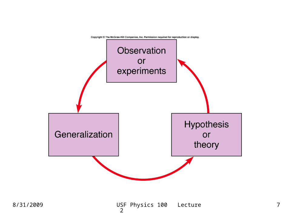
Functional Relationships

Mathematical representation of the relationship between quantities.y = f(x)

y: dependent variable, ordinatex: independent variable, abscissa

f

x input y output


As many forms as there are mathematical functions

Forms of primary concern to us:

Directly proportionalInversely proportionalProportional to the squareInversely proportional to the square


A. Directly proportional

Also called “linear”Form: y = mx + b

x

y

Example: x = elapsed timey = distance traveled

thenm = velocity or speedb = initial distance or starting distance


B. Directly Proportional to the SquareForm: y = mx2

0

50

100

150

200

250

-20 -15 -10 -5 0 5 10 15 20

Series1

Example:y = area of a squarex = length of square’s edge

m = 1 for this case


C. Inversely Proportional

Form: y = m/x

y

x

Example:y = time to travel a distancex = velocity or speed

m = 1 for this case


D. Inversely Proportional to the Square

Form: y = m/x2

y

x

Example:y = gravitational attraction between m1 and m2.x = separation

m = -Gm1m2

1 2

2

m mF G

r

m/x


Polynomial

2 110 1 2 11

ni

ii n

n nn nn nn n

y m x

m mm m x m x m x m x

x x

20 0

1

2x t x v t at

Example: Motion in 1-D


Calculus vs. Non-Calculus Notation

x

yExample: x = elapsed timey = distance traveled

thenm = velocity or speedb = initial distance or starting distance

You do not need calculus for this course but sometimes I get sloppy with notation.

y dym

x dx

For a linear function like the above


dy

dxis called the derivative of y w.r.t. x

0

50

100

150

200

250

-20 -15 -10 -5 0 5 10 15 20

Series1

Now consider a non-linear function like y = x2

There is a slope at each point of the curve but it is continually changing


0

50

100

150

200

250

-20 -15 -10 -5 0 5 10 15 20

Series1

x

y

0limx

dy y

dx x

y

x

is the average slope over the range shown.


Area under a curvef(x)

xx

A f x x


5

05

limi

i ixi

A f x dx f x x

ii

A f x x xi

5

5

f x dx is called the integral of f(x) from x = -5 to 5


Measurement and ErrorsThere is no such thing as an “exact” measurement.One must supply information about the reliability or exactness of a quoted measurement.Significant Figures: Inclusion of a particular number of digits => except possibly for the last one they are all known to be correct.

e. g. page is 11 inches but probably not 11.000000 inches.11.000000”=> your measurement is good to about 10-6” and probably not as bad as 11.000005”


Another Way: Specifically call out limits of uncertainty.

e. g. 4.0 ± 0.2 cmbest estimate is 4.0 cm and true value is

“likely” to be within 0.2 cm of this estimate

Can also be written as 4.0 ± 5% cm or 4.0 cm ± 5%


Statistical or Random ErrorsFire a perfect shotgun at a targetSights aligned and you are a perfect shot.

Result: symmetrical pattern of hits centered on target. Gaussian distribution of hits. Average is location of target.

N

r

Repetition of experiment can reduce the effects of these types of errors.


.

Systematic ErrorsNow knock shotgun’s sights out of line

Result: Same sort of pattern as before but pattern as a whole is shifted systematically.

N

r

Systematic errors can be corrected if they are understood. e. g. If shotgun shoots high and right, aim low and left.


Mistakes

Mistake in experimental procedure.

e. g. Aim the shotgun at the wrong place



Total of 13 subjects divided into a 2 bin distribution.½ (6.5) subjects’ BP lowered½(6.5) subjects’ BP remained high.

NPoisson statistics: Error (random) in counting N events is

Numbers should be quoted: 6.5 ± 2.5

Danger of small statistical universes


Trigonometry Review

hypotenuse

adjacent

opposite

oppositesin

hypotenuse

adjacentcos

hypotenuse

oppositetan

adjacent

Pythagorian Theorem:

(hypotenuse)2 = (opposite)2 + (adjacent)2

Trigonometric Functions:

adjacentcot

opposite

hypotenusecsc

adjacent

hypotenusesec

opposite

2 2sin cos 1


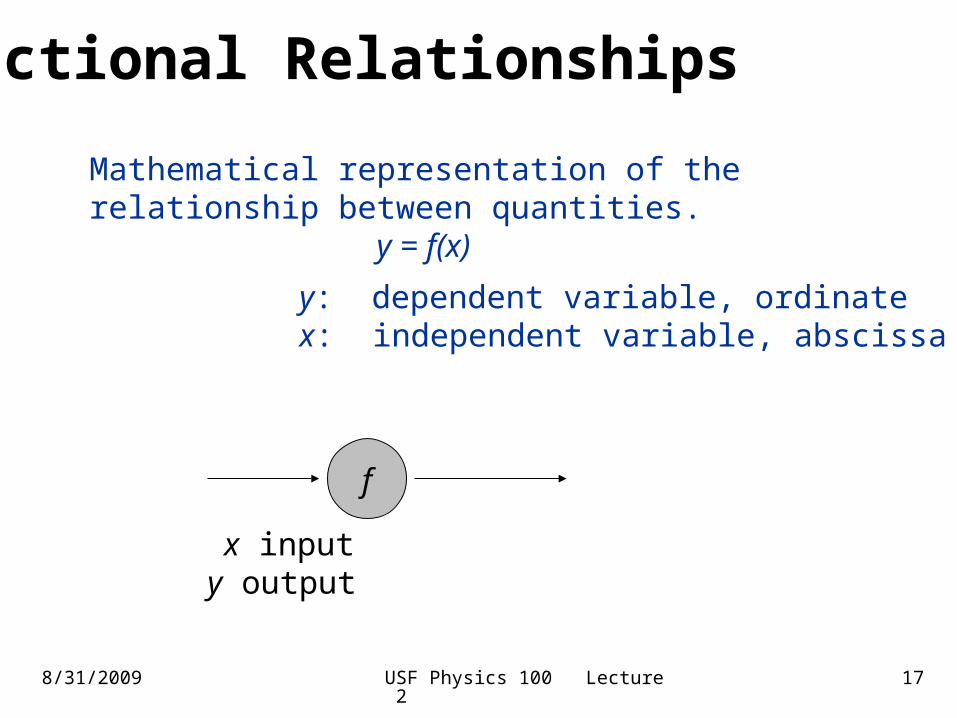
Vectors

Scalars: Magnitude only e. g. mass, energy, temperature

Vectors: Magnitude and direction e. g. force, momentum

Graphically:Length represents magnitudeOrientation represents direction


Graphical Addition of Vectors

The parallelogram of forces

C A B

B

A

C


Component Addition of Vectors

x-axis

y-axis

Ax

Ay

A

Ax = A cos A

Ay = A sin A

Similarly, Bx = B cos B, etc.

2 2 magnitude of , x yA A A A A

C A B

A


Add the componentsCx = Ax + Bx

Cy = Ay + By

2 2 magnitude of x yC C C C

1 tan tan

Angle whose tangent is

y yC

x x

y

x

C CArc

C C

C

C

8/31/2009USF Physics 100 Lecture 21 Physics 100 Fall 2009 Lecture 2 Getting Started .

Documents

usf physics

web lecture

scientific method physics

usf wiki

ca slide

x10 b2

scientific theory

x10 b1b2 exponents