8. Seismic Structure: Mantlepress-files.anu.edu.au/downloads/press/n4442/pdf/ch08.pdf · from seismic surface wave tomography. This approach exploits the large amplitude Rayleigh

The Australian Continent: A Geophysical Synthesis— Seismic Structure: Mantle

8. Seismic Structure: Mantle

A distinctive feature of the structure in the mantle component of the lithosphere

beneath the Australian continent is a strong contrast in character between the

Precambrian areas in the west and centre and the younger east. The west has a

much thicker lithosphere with rather high shear wavespeeds, whereas beneath

the Phanerozoic east the lithosphere is quite thin and there is a prominent zone

of lowered seismic wavespeeds below.

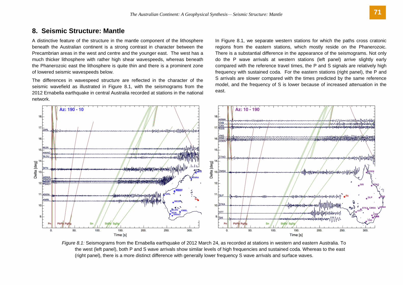
The differences in wavespeed structure are reflected in the character of the

seismic wavefield as illustrated in Figure 8.1, with the seismograms from the

2012 Ernabella earthquake in central Australia recorded at stations in the national

network.

In Figure 8.1, we separate western stations for which the paths cross cratonic

regions from the eastern stations, which mostly reside on the Phanerozoic.

There is a substantial difference in the appearance of the seismograms. Not only

do the P wave arrivals at western stations (left panel) arrive slightly early

compared with the reference travel times, the P and S signals are relatively high

frequency with sustained coda. For the eastern stations (right panel), the P and

S arrivals are slower compared with the times predicted by the same reference

model, and the frequency of S is lower because of increased attenuation in the

east.

Figure 8.1: Seismograms from the Ernabella earthquake of 2012 March 24, as recorded at stations in western and eastern Australia. To

the west (left panel), both P and S wave arrivals show similar levels of high frequencies and sustained coda. Whereas to the east

(right panel), there is a more distinct difference with generally lower frequency S wave arrivals and surface waves.

71

The Australian Continent: A Geophysical Synthesis — Seismic Structure: Mantle

8.1 Mantle Lithosphere

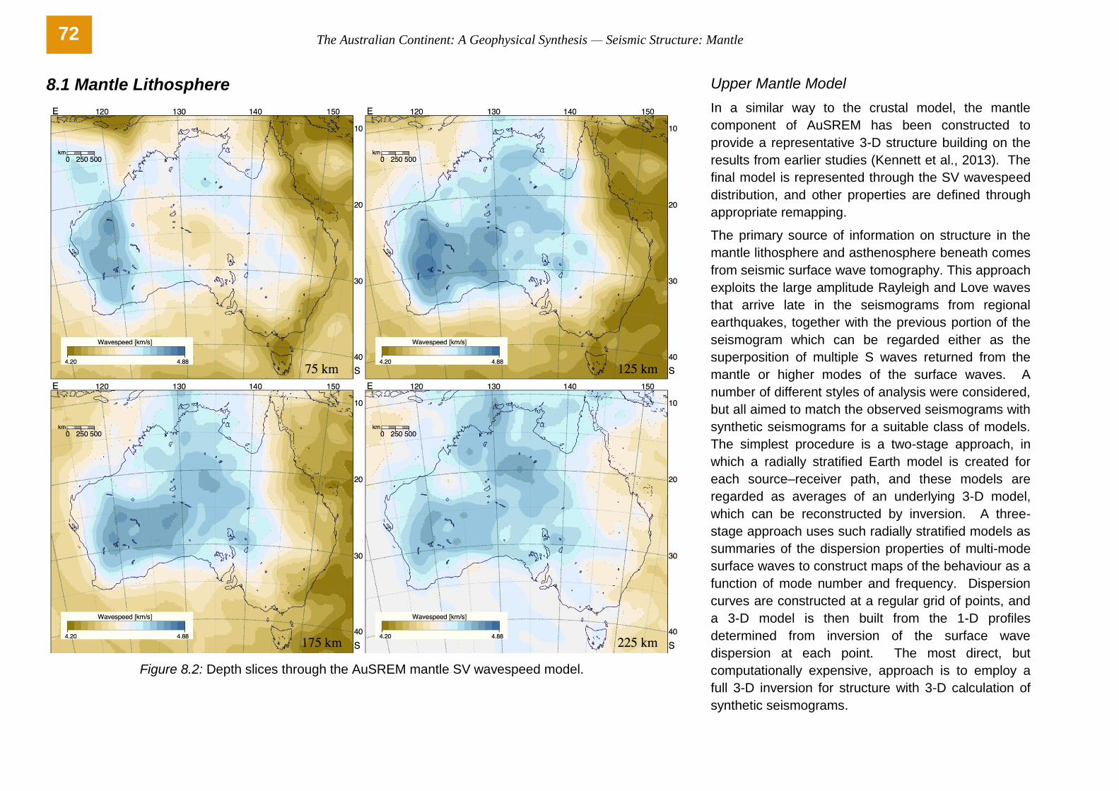
Figure 8.2: Depth slices through the AuSREM mantle SV wavespeed model.

Upper Mantle Model

In a similar way to the crustal model, the mantle

component of AuSREM has been constructed to

provide a representative 3-D structure building on the

results from earlier studies (Kennett et al., 2013). The

final model is represented through the SV wavespeed

distribution, and other properties are defined through

appropriate remapping.

The primary source of information on structure in the

mantle lithosphere and asthenosphere beneath comes

from seismic surface wave tomography. This approach

exploits the large amplitude Rayleigh and Love waves

that arrive late in the seismograms from regional

earthquakes, together with the previous portion of the

seismogram which can be regarded either as the

superposition of multiple S waves returned from the

mantle or higher modes of the surface waves. A

number of different styles of analysis were considered,

but all aimed to match the observed seismograms with

synthetic seismograms for a suitable class of models.

The simplest procedure is a two-stage approach, in

which a radially stratified Earth model is created for

each source–receiver path, and these models are

regarded as averages of an underlying 3-D model,

which can be reconstructed by inversion. A three-

stage approach uses such radially stratified models as

summaries of the dispersion properties of multi-mode

surface waves to construct maps of the behaviour as a

function of mode number and frequency. Dispersion

curves are constructed at a regular grid of points, and

a 3-D model is then built from the 1-D profiles

determined from inversion of the surface wave

dispersion at each point. The most direct, but

computationally expensive, approach is to employ a

full 3-D inversion for structure with 3-D calculation of

synthetic seismograms.

72


SV Wavespeed:

The AuSREM SV wavespeed model represents a

balance between these different styles of analysis,

which produce very similar results for the long-

wavelength component of the wavespeed model

(Fichtner et al., 2012), but differ more at shorter

wavelengths. In Figure 8.2 we display depth slices at

50 km intervals through the portion of the SV

wavespeed AuSREM model that lies beneath the

Australian continent. It is immediately apparent that

rather high shear wavespeeds persist to a depth of

225 km – indicative of a thick cratonic lithosphere. On

the eastern margin of the continent we encounter quite

low shear wavespeeds in the depth range from 75–

175 km, associated with thinner lithosphere and a

consequent shallow asthenosphere. The Tasman Sea

region displays quite low SV wavespeeds (down to 4.2

km/s), probably as a result of residual heat left from

failed rifting around 80 Ma.

Compared with the Western Australian Craton, the

shear wavespeeds in central Australia are somewhat

lower at 75 km depth. However, by 125 km depth fast

wavespeeds occupy the same zone. The seismic

wavespeeds in the Gawler Craton are noticeably lower

than in the other cratonic components, possibly as a

result of thermal alteration in the emplacement of

extensive Proterozoic volcanics in this region.

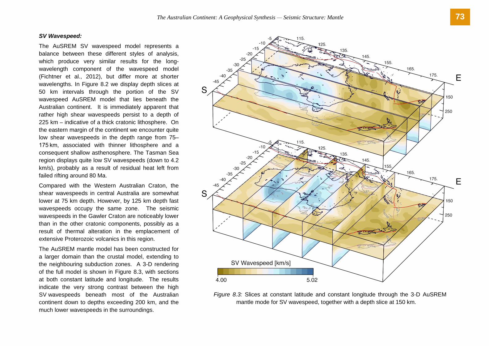
The AuSREM mantle model has been constructed for

a larger domain than the crustal model, extending to

the neighbouring subduction zones. A 3-D rendering

of the full model is shown in Figure 8.3, with sections

at both constant latitude and longitude. The results

indicate the very strong contrast between the high

SV wavespeeds beneath most of the Australian

continent down to depths exceeding 200 km, and the

much lower wavespeeds in the surroundings.

Figure 8.3: Slices at constant latitude and constant longitude through the 3-D AuSREM

mantle mode for SV wavespeed, together with a depth slice at 150 km.

73


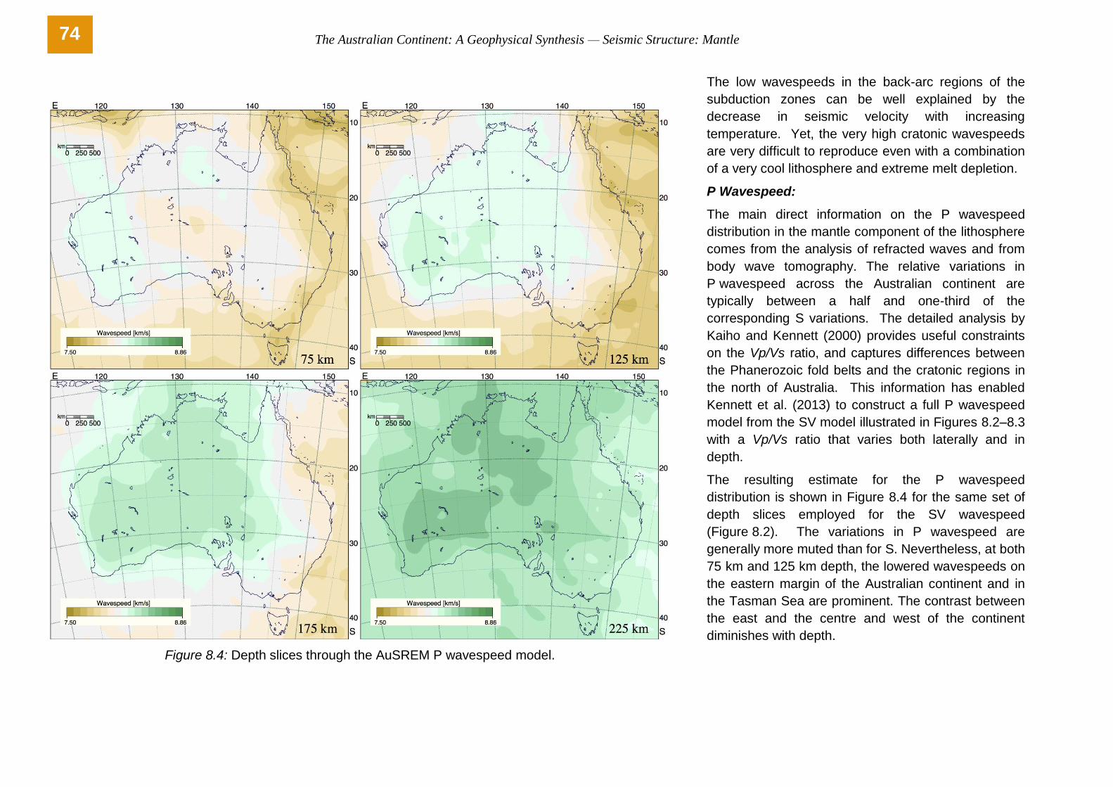
Figure 8.4: Depth slices through the AuSREM P wavespeed model.

The low wavespeeds in the back-arc regions of the

subduction zones can be well explained by the

decrease in seismic velocity with increasing

temperature. Yet, the very high cratonic wavespeeds

are very difficult to reproduce even with a combination

of a very cool lithosphere and extreme melt depletion.

P Wavespeed:

The main direct information on the P wavespeed

distribution in the mantle component of the lithosphere

comes from the analysis of refracted waves and from

body wave tomography. The relative variations in

P wavespeed across the Australian continent are

typically between a half and one-third of the

corresponding S variations. The detailed analysis by

Kaiho and Kennett (2000) provides useful constraints

on the Vp/Vs ratio, and captures differences between

the Phanerozoic fold belts and the cratonic regions in

the north of Australia. This information has enabled

Kennett et al. (2013) to construct a full P wavespeed

model from the SV model illustrated in Figures 8.2–8.3

with a Vp/Vs ratio that varies both laterally and in

depth.

The resulting estimate for the P wavespeed

distribution is shown in Figure 8.4 for the same set of

depth slices employed for the SV wavespeed

(Figure 8.2). The variations in P wavespeed are

generally more muted than for S. Nevertheless, at both

75 km and 125 km depth, the lowered wavespeeds on

the eastern margin of the Australian continent and in

the Tasman Sea are prominent. The contrast between

the east and the centre and west of the continent

diminishes with depth.

74


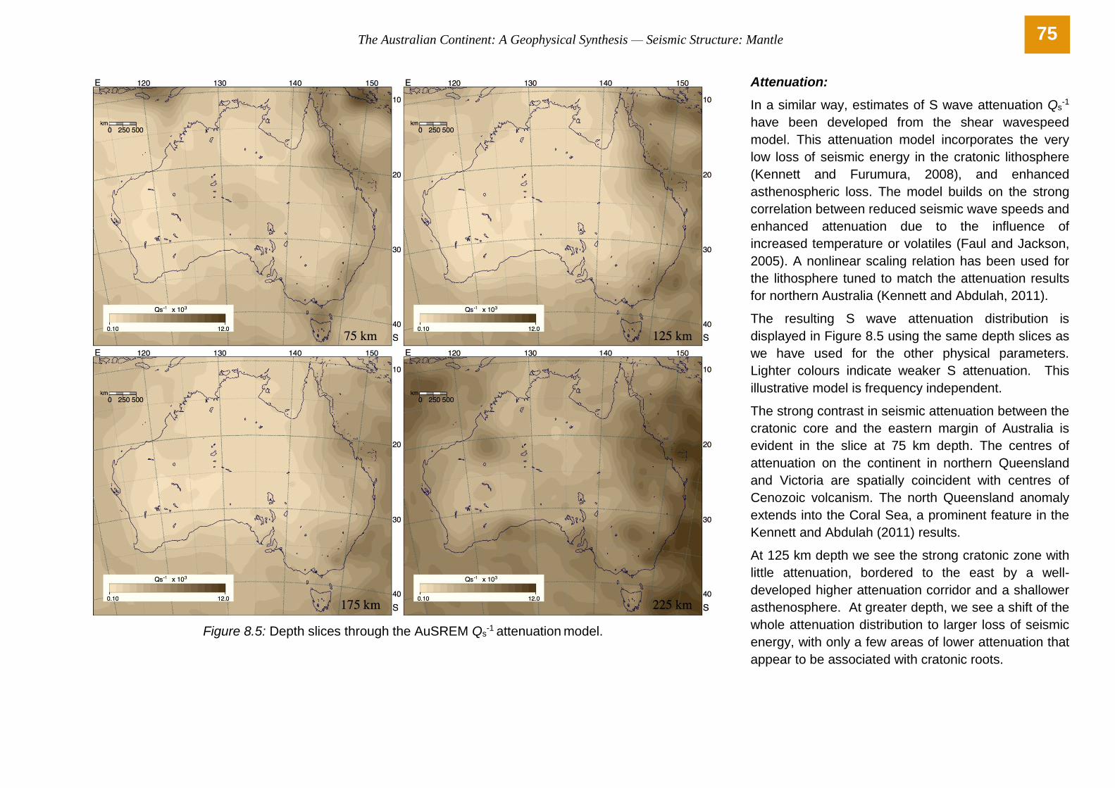
Figure 8.5: Depth slices through the AuSREM Qs-1 attenuation model.

Attenuation:

In a similar way, estimates of S wave attenuation Qs-1

have been developed from the shear wavespeed

model. This attenuation model incorporates the very

low loss of seismic energy in the cratonic lithosphere

(Kennett and Furumura, 2008), and enhanced

asthenospheric loss. The model builds on the strong

correlation between reduced seismic wave speeds and

enhanced attenuation due to the influence of

increased temperature or volatiles (Faul and Jackson,

2005). A nonlinear scaling relation has been used for

the lithosphere tuned to match the attenuation results

for northern Australia (Kennett and Abdulah, 2011).

The resulting S wave attenuation distribution is

displayed in Figure 8.5 using the same depth slices as

we have used for the other physical parameters.

Lighter colours indicate weaker S attenuation. This

illustrative model is frequency independent.

The strong contrast in seismic attenuation between the

cratonic core and the eastern margin of Australia is

evident in the slice at 75 km depth. The centres of

attenuation on the continent in northern Queensland

and Victoria are spatially coincident with centres of

Cenozoic volcanism. The north Queensland anomaly

extends into the Coral Sea, a prominent feature in the

Kennett and Abdulah (2011) results.

At 125 km depth we see the strong cratonic zone with

little attenuation, bordered to the east by a well-

developed higher attenuation corridor and a shallower

asthenosphere. At greater depth, we see a shift of the

whole attenuation distribution to larger loss of seismic

energy, with only a few areas of lower attenuation that

appear to be associated with cratonic roots.

75


Transition from Lithosphere to Asthenosphere

The lithosphere forms the outer, relatively rigid shell of the Earth. It is underlain

by mantle material participating in mantle convection: this rheologically weak

zone is referred to as the asthenosphere (Figure 8.6). There are many

contrasting definitions for the base of the lithosphere associated with different

aspects of the physical properties of Earth materials (Artemieva, 2011). The

situation is rendered more complex by the strong heterogeneity of the

lithosphere, both laterally and vertically, and the variety of different geophysical

and geochemical proxies that have been employed to define a specific

lithosphere–asthenosphere boundary (LAB) rather than a rheological change.

Except in a few circumstances, there is no sharp, distinctive discontinuity and it is

more appropriate to refer to a lithosphere–asthenosphere transition (LAT).

The transition from the conductive to the convective regime provides a thermal

definition of the lithosphere, e.g. through the depth to a constant geotherm (e.g.

1300°C) or the intersection of the extrapolation of the conductive geotherm to

intersect the mantle adiabat. Mantle xenoliths are employed to provide a

petrological definition based on the transition from depleted, lithospheric minerals

to a more fertile, asthenospheric, composition, often using proxies such as garnet

concentrations. The temperature conditions for the transition are similar to those

for the thermal case. The change in mineral properties has a stronger effect on

the Vp/Vs ratio than on the velocity variations themselves and so the position of

change in the Vp/Vs ratio with depth can be interpreted as the base of the

petrological lithosphere.

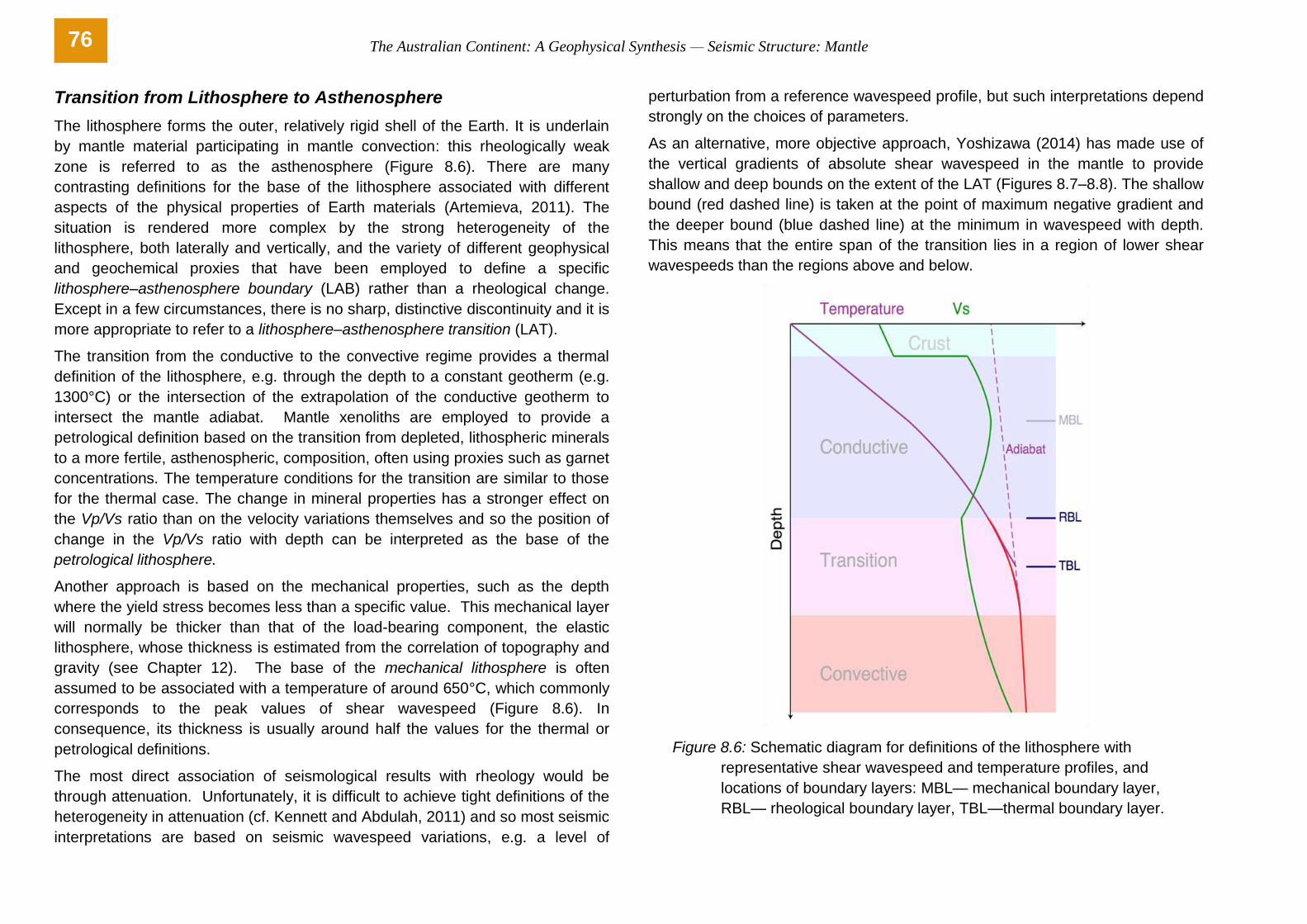
Another approach is based on the mechanical properties, such as the depth

where the yield stress becomes less than a specific value. This mechanical layer

will normally be thicker than that of the load-bearing component, the elastic

lithosphere, whose thickness is estimated from the correlation of topography and

gravity (see Chapter 12). The base of the mechanical lithosphere is often

assumed to be associated with a temperature of around 650°C, which commonly

corresponds to the peak values of shear wavespeed (Figure 8.6). In

consequence, its thickness is usually around half the values for the thermal or

petrological definitions.

The most direct association of seismological results with rheology would be

through attenuation. Unfortunately, it is difficult to achieve tight definitions of the

heterogeneity in attenuation (cf. Kennett and Abdulah, 2011) and so most seismic

interpretations are based on seismic wavespeed variations, e.g. a level of

perturbation from a reference wavespeed profile, but such interpretations depend

strongly on the choices of parameters.

As an alternative, more objective approach, Yoshizawa (2014) has made use of

the vertical gradients of absolute shear wavespeed in the mantle to provide

shallow and deep bounds on the extent of the LAT (Figures 8.7–8.8). The shallow

bound (red dashed line) is taken at the point of maximum negative gradient and

the deeper bound (blue dashed line) at the minimum in wavespeed with depth.

This means that the entire span of the transition lies in a region of lower shear

wavespeeds than the regions above and below.

Figure 8.6: Schematic diagram for definitions of the lithosphere with

representative shear wavespeed and temperature profiles, and

locations of boundary layers: MBL— mechanical boundary layer,

RBL— rheological boundary layer, TBL—thermal boundary layer.

76


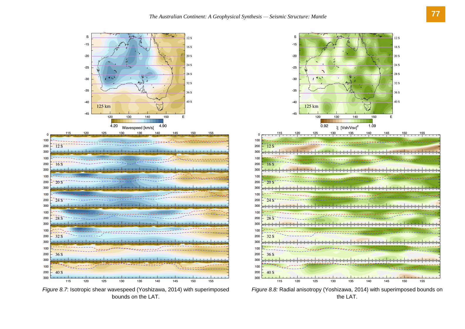
Figure 8.7: Isotropic shear wavespeed (Yoshizawa, 2014) with superimposed

bounds on the LAT.

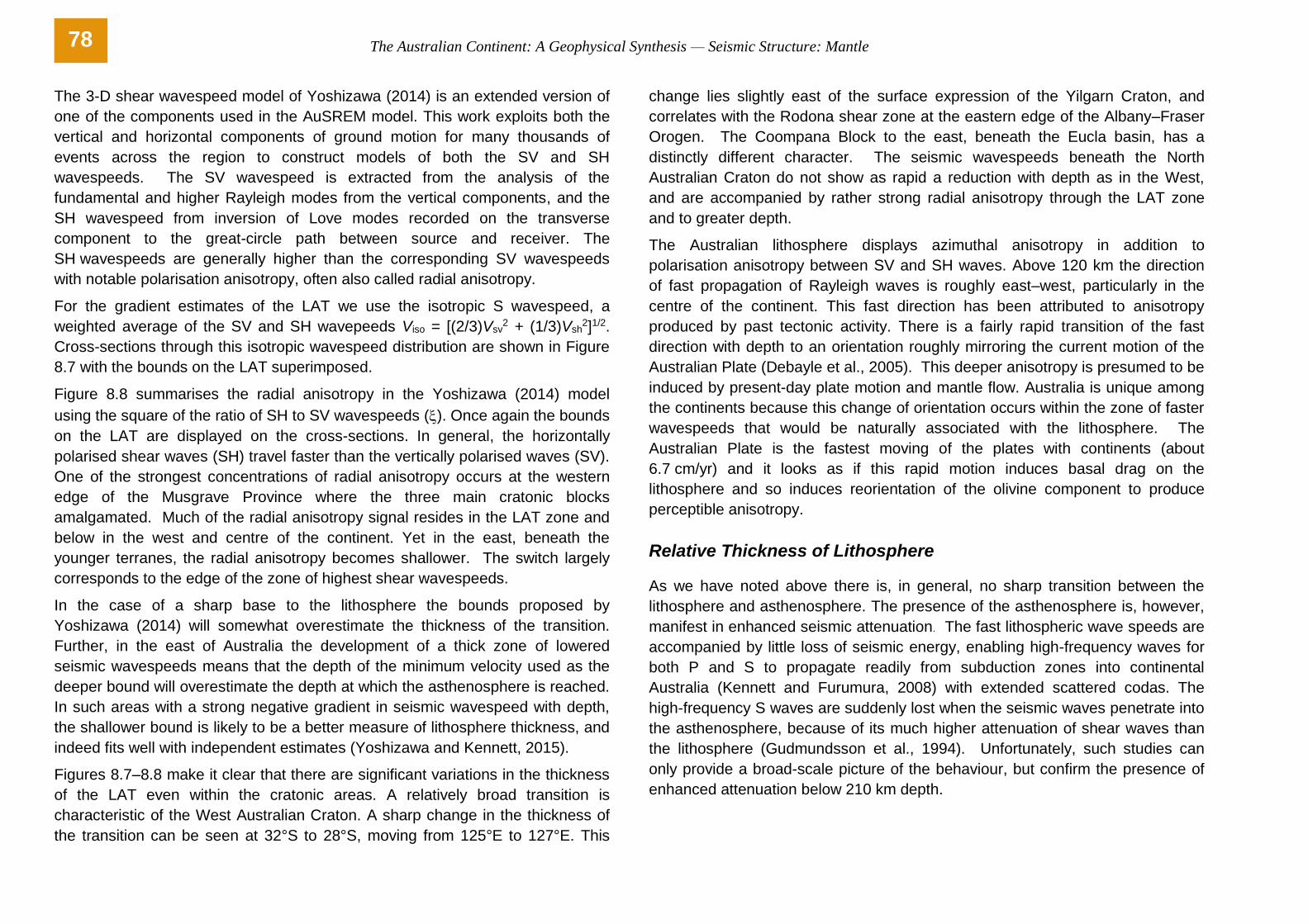
Figure 8.8: Radial anisotropy (Yoshizawa, 2014) with superimposed bounds on

the LAT.

77


The 3-D shear wavespeed model of Yoshizawa (2014) is an extended version of

one of the components used in the AuSREM model. This work exploits both the

vertical and horizontal components of ground motion for many thousands of

events across the region to construct models of both the SV and SH

wavespeeds. The SV wavespeed is extracted from the analysis of the

fundamental and higher Rayleigh modes from the vertical components, and the

SH wavespeed from inversion of Love modes recorded on the transverse

component to the great-circle path between source and receiver. The

SH wavespeeds are generally higher than the corresponding SV wavespeeds

with notable polarisation anisotropy, often also called radial anisotropy.

For the gradient estimates of the LAT we use the isotropic S wavespeed, a

weighted average of the SV and SH wavepeeds Viso = [(2/3)Vsv2 + (1/3)Vsh

2]1/2.

Cross-sections through this isotropic wavespeed distribution are shown in Figure

8.7 with the bounds on the LAT superimposed.

Figure 8.8 summarises the radial anisotropy in the Yoshizawa (2014) model

using the square of the ratio of SH to SV wavespeeds (). Once again the bounds

on the LAT are displayed on the cross-sections. In general, the horizontally

polarised shear waves (SH) travel faster than the vertically polarised waves (SV).

One of the strongest concentrations of radial anisotropy occurs at the western

edge of the Musgrave Province where the three main cratonic blocks

amalgamated. Much of the radial anisotropy signal resides in the LAT zone and

below in the west and centre of the continent. Yet in the east, beneath the

younger terranes, the radial anisotropy becomes shallower. The switch largely

corresponds to the edge of the zone of highest shear wavespeeds.

In the case of a sharp base to the lithosphere the bounds proposed by

Yoshizawa (2014) will somewhat overestimate the thickness of the transition.

Further, in the east of Australia the development of a thick zone of lowered

seismic wavespeeds means that the depth of the minimum velocity used as the

deeper bound will overestimate the depth at which the asthenosphere is reached.

In such areas with a strong negative gradient in seismic wavespeed with depth,

the shallower bound is likely to be a better measure of lithosphere thickness, and

indeed fits well with independent estimates (Yoshizawa and Kennett, 2015).

Figures 8.7–8.8 make it clear that there are significant variations in the thickness

of the LAT even within the cratonic areas. A relatively broad transition is

characteristic of the West Australian Craton. A sharp change in the thickness of

the transition can be seen at 32°S to 28°S, moving from 125°E to 127°E. This

change lies slightly east of the surface expression of the Yilgarn Craton, and

correlates with the Rodona shear zone at the eastern edge of the Albany–Fraser

Orogen. The Coompana Block to the east, beneath the Eucla basin, has a

distinctly different character. The seismic wavespeeds beneath the North

Australian Craton do not show as rapid a reduction with depth as in the West,

and are accompanied by rather strong radial anisotropy through the LAT zone

and to greater depth.

The Australian lithosphere displays azimuthal anisotropy in addition to

polarisation anisotropy between SV and SH waves. Above 120 km the direction

of fast propagation of Rayleigh waves is roughly east–west, particularly in the

centre of the continent. This fast direction has been attributed to anisotropy

produced by past tectonic activity. There is a fairly rapid transition of the fast

direction with depth to an orientation roughly mirroring the current motion of the

Australian Plate (Debayle et al., 2005). This deeper anisotropy is presumed to be

induced by present-day plate motion and mantle flow. Australia is unique among

the continents because this change of orientation occurs within the zone of faster

wavespeeds that would be naturally associated with the lithosphere. The

Australian Plate is the fastest moving of the plates with continents (about

6.7 cm/yr) and it looks as if this rapid motion induces basal drag on the

lithosphere and so induces reorientation of the olivine component to produce

perceptible anisotropy.

Relative Thickness of Lithosphere

As we have noted above there is, in general, no sharp transition between the

lithosphere and asthenosphere. The presence of the asthenosphere is, however,

manifest in enhanced seismic attenuation. The fast lithospheric wave speeds are

accompanied by little loss of seismic energy, enabling high-frequency waves for

both P and S to propagate readily from subduction zones into continental

Australia (Kennett and Furumura, 2008) with extended scattered codas. The

high-frequency S waves are suddenly lost when the seismic waves penetrate into

the asthenosphere, because of its much higher attenuation of shear waves than

the lithosphere (Gudmundsson et al., 1994). Unfortunately, such studies can

only provide a broad-scale picture of the behaviour, but confirm the presence of

enhanced attenuation below 210 km depth.

78


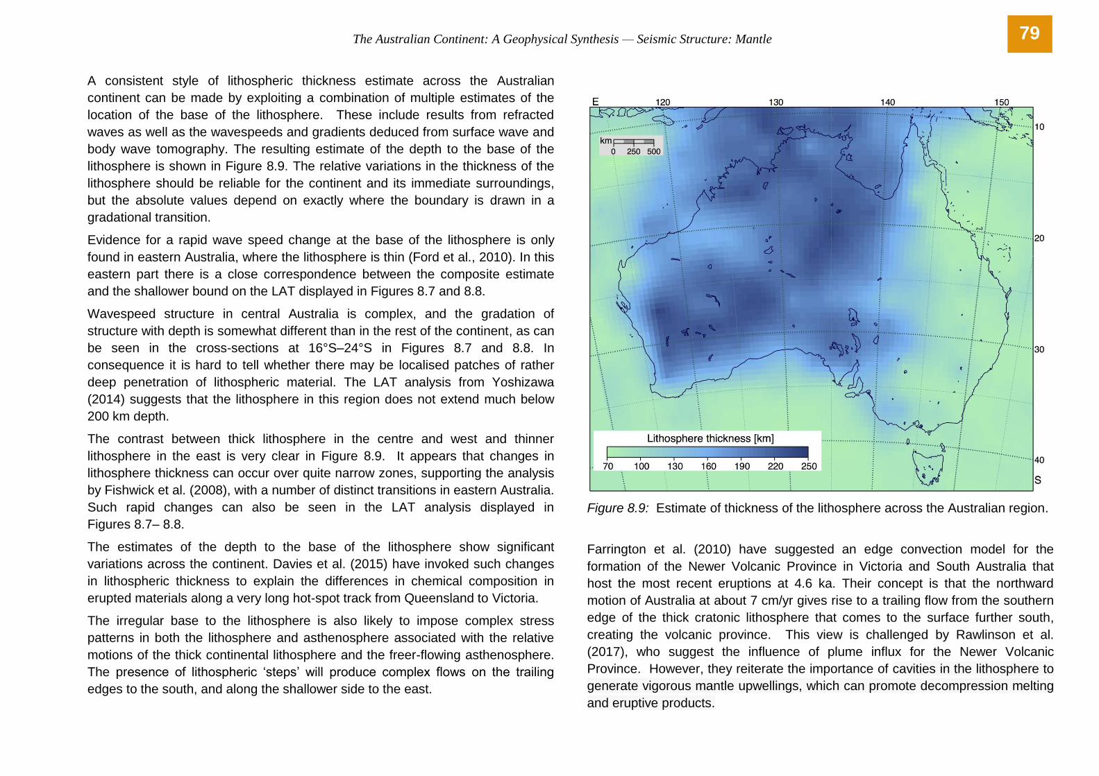
A consistent style of lithospheric thickness estimate across the Australian

continent can be made by exploiting a combination of multiple estimates of the

location of the base of the lithosphere. These include results from refracted

waves as well as the wavespeeds and gradients deduced from surface wave and

body wave tomography. The resulting estimate of the depth to the base of the

lithosphere is shown in Figure 8.9. The relative variations in the thickness of the

lithosphere should be reliable for the continent and its immediate surroundings,

but the absolute values depend on exactly where the boundary is drawn in a

gradational transition.

Evidence for a rapid wave speed change at the base of the lithosphere is only

found in eastern Australia, where the lithosphere is thin (Ford et al., 2010). In this

eastern part there is a close correspondence between the composite estimate

and the shallower bound on the LAT displayed in Figures 8.7 and 8.8.

Wavespeed structure in central Australia is complex, and the gradation of

structure with depth is somewhat different than in the rest of the continent, as can

be seen in the cross-sections at 16°S–24°S in Figures 8.7 and 8.8. In

consequence it is hard to tell whether there may be localised patches of rather

deep penetration of lithospheric material. The LAT analysis from Yoshizawa

(2014) suggests that the lithosphere in this region does not extend much below

200 km depth.

The contrast between thick lithosphere in the centre and west and thinner

lithosphere in the east is very clear in Figure 8.9. It appears that changes in

lithosphere thickness can occur over quite narrow zones, supporting the analysis

by Fishwick et al. (2008), with a number of distinct transitions in eastern Australia.

Such rapid changes can also be seen in the LAT analysis displayed in

Figures 8.7– 8.8.

The estimates of the depth to the base of the lithosphere show significant

variations across the continent. Davies et al. (2015) have invoked such changes

in lithospheric thickness to explain the differences in chemical composition in

erupted materials along a very long hot-spot track from Queensland to Victoria.

The irregular base to the lithosphere is also likely to impose complex stress

patterns in both the lithosphere and asthenosphere associated with the relative

motions of the thick continental lithosphere and the freer-flowing asthenosphere.

The presence of lithospheric ‘steps’ will produce complex flows on the trailing

edges to the south, and along the shallower side to the east.

Figure 8.9: Estimate of thickness of the lithosphere across the Australian region.

Farrington et al. (2010) have suggested an edge convection model for the

formation of the Newer Volcanic Province in Victoria and South Australia that

host the most recent eruptions at 4.6 ka. Their concept is that the northward

motion of Australia at about 7 cm/yr gives rise to a trailing flow from the southern

edge of the thick cratonic lithosphere that comes to the surface further south,

creating the volcanic province. This view is challenged by Rawlinson et al.

(2017), who suggest the influence of plume influx for the Newer Volcanic

Province. However, they reiterate the importance of cavities in the lithosphere to

generate vigorous mantle upwellings, which can promote decompression melting

and eruptive products.

79


8.2 Uppermost Mantle

The uppermost part of the lithospheric mantle

immediately below the crust is not well constrained by

surface wave studies, because of potential influence

from the crust on the results. Fortunately, alternative

probes exist through the properties of the regional

phases Pn and Sn, which travel beneath the Moho and

are sensitive to the velocity structure and gradients in

this region. Examples of such Pn and Sn arrivals are

illustrated in the seismograms of Figure 8.1 for the

2012 Ernabella event. In the cratonic regions of the

continent, the onsets of Pn and Sn have rather higher

frequencies. This makes Pn a rather sharp arrival, but

Sn is more difficult to pick against a background of

high-frequency P wave coda.

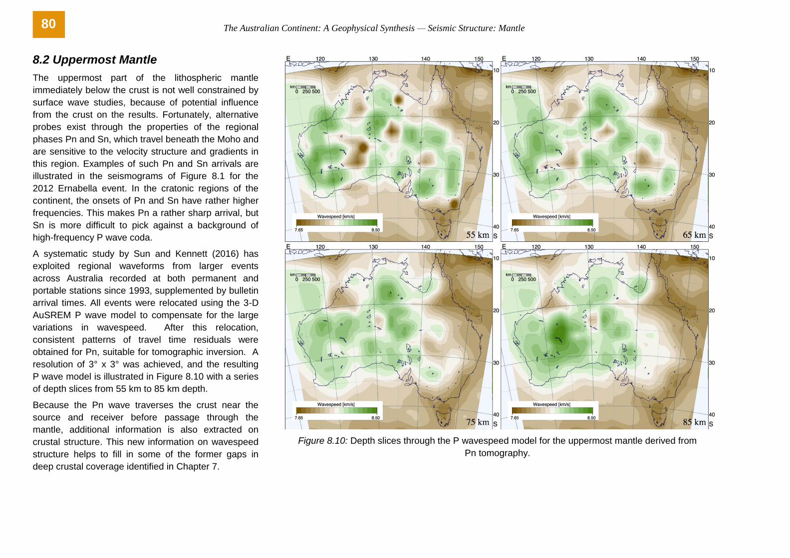
A systematic study by Sun and Kennett (2016) has

exploited regional waveforms from larger events

across Australia recorded at both permanent and

portable stations since 1993, supplemented by bulletin

arrival times. All events were relocated using the 3-D

AuSREM P wave model to compensate for the large

variations in wavespeed. After this relocation,

consistent patterns of travel time residuals were

obtained for Pn, suitable for tomographic inversion. A

resolution of 3° x 3° was achieved, and the resulting

P wave model is illustrated in Figure 8.10 with a series

of depth slices from 55 km to 85 km depth.

Because the Pn wave traverses the crust near the

source and receiver before passage through the

mantle, additional information is also extracted on

crustal structure. This new information on wavespeed

structure helps to fill in some of the former gaps in

deep crustal coverage identified in Chapter 7.

Figure 8.10: Depth slices through the P wavespeed model for the uppermost mantle derived from

Pn tomography.

80


In the depth slice at 55 km the prominent slow anomalies in P wave velocities are

associated with the influence of rather thick crust. Throughout the depth range of

55–85 km in Figure 8.10, the slowest velocities in the uppermost mantle are

found along the eastern margin of the Australian continent beneath the

Phanerozoic orogenic belts, with links to Neogene volcanism. Path coverage is

limited in Arnhem Land and the northeast of Australia, due to paucity of sources

and seismic stations, so that wavespeed variations may be underestimated in

these areas.

Across much of the continent, the P wavespeed in the uppermost mantle is a little

faster than in AuSREM, suggesting the need for some increase in the Vp∕Vs ratio

compared with AuSREM. The fastest Pn wavespeeds are found in the cratonic

areas, but we note significant substructures in the P wavespeed beneath the

cratons. Rather high P wavespeeds are encountered beneath the Pilbara and

Yilgarn cratons, and in patches of the North Australian Craton. The South

Australian Craton shows more subdued velocity variations with localised high

Pn wavespeeds in the neighbourhood of the Curnamona Province and in the

Gawler region to the east. A persistent patch of lowered wavespeeds is found

near Alice Springs.

Between the West Australian and South Australian cratons, there are variations

in the P wavespeed beneath the Eucla basin that appear to link to distinct

lithospheric blocks with their own signatures of physical properties.

At both 70 km and 85 km there is a reduced P wavespeed anomaly associated

with the northern part of the Canning Basin. This basin has an active tectonic

history over a long interval, with significant accumulations of sediments and minor

oil production.

Similar patterns of variation are found for S wavespeed from the tomographic

inversion of Sn travel times. The Vp/Vs ratio lies mostly in the range 1.7 to 1.825

with a relatively smooth variation. Relatively low S wavespeeds are found just

beneath the crust in the vicinity of Alice Springs, and this anomaly persists

somewhat to greater depth with an extension to the south along the western edge

of the South Australian Craton. Low S velocities are found at 18°S on the

eastern margin of the continent extending to about 65 km depth; this feature

extends both north and south at shallower depth.

8.3 Nature of Lithospheric Structure

The reflection transects displayed in Chapter 7 indicate the complexity of crustal

structure, with generally stronger variability in structure at the base of the crust.

However, at the frequencies employed in reflection seismology the mantle

normally appears to be rather bland with no apparent reflectors. Nonetheless,

there is significant evidence for the existence of heterogeneity within the mantle

component of lithosphere, but at larger scales.

The broadest-scale features are well mapped by exploiting the properties of

surface waves and multiply reflected S body waves as we have seen in

Section 8.1. Body-wave tomography exploiting relatively dense deployments of

portable seismic recorders provides information on the lithospheric mantle at

shorter scales. Potential horizontal resolution is limited by station spacing

(Rawlinson et al., 2014), but vertical smearing due to the relatively narrow cone

of incoming rays also limits resolution in the upper mantle.

The suite of portable instrument deployments in the WOMBAT project in

southeastern Australia reveals the presence of considerable complexity in and

beneath the crust (e.g. Rawlinson et al., 2016), with variations down to the

available sampling of 50 km. The presence of much finer-scale structure in the

mantle is indicated by long trains of high-frequency P and S waves following the

phases Pn and Sn refracted back from the mantle, as in the seismograms shown

in Figure 8.1 for continental paths within Australia. The nature of this extended

high-frequency coda, particularly for paths within the Precambrian domains,

requires some form of distributed heterogeneity through the lithosphere (Kennett

and Furumura, 2008).

Evidence for discontinuities in physical properties within the mantle component of

the lithosphere comes from studies of the structure in the vicinity of seismic

stations. A commonly used approach exploits the wave conversions and

reflections associated with the major seismic phases from distant earthquakes to

construct receiver functions. Incident S waves have been favoured for

discontinuity studies because the converted P waves arrive as precursors to S,

though relatively low frequencies have to be used which limits vertical resolution.

One of the striking features in S wave receiver function analysis for the Australian

cratons is clear signals of discontinuities in the mid-lithosphere at around

70–90 km (Ford et al., 2010), which may indicate a rapid drop in seismic velocity

or a change in the character of radial anisotropy in the middle part of the

continental lithosphere where the wavespeed is generally at its fastest. The

81


estimated depth of the enigmatic mid-lithosphere discontinuity (MLD) from

receiver functions corresponds well with a rapid change in the strength of radial

anisotropy derived from surface waves (Yoshizawa and Kennett, 2015).

An additional constraint on the nature of lithospheric heterogeneity comes from

observations of high-frequency P wave reflectivity profiles derived from the

autocorrelograms of vertical component records at seismic stations (Kennett,

2015; Sun et al., 2018). These P reflectivity profiles suggest vertical changes in

the character of the fine-scale structures in the Australian continent, indicating

stronger reflectivity in the crust and upper lithosphere underneath the cratons.

Indications of mid-lithospheric discontinuities are provided by distinct changes in

the frequency content of the reflectivity as a function of time.

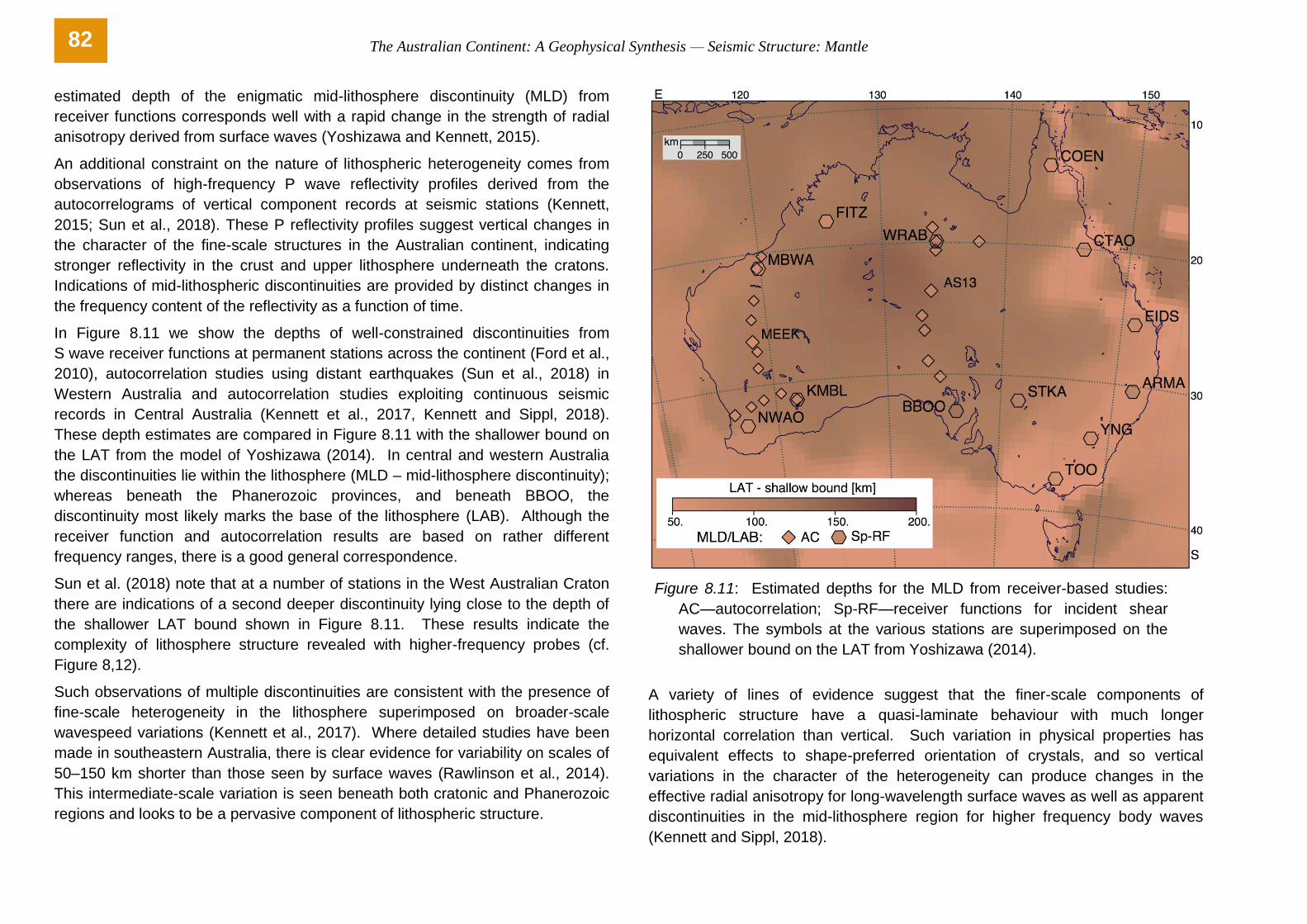
In Figure 8.11 we show the depths of well-constrained discontinuities from

S wave receiver functions at permanent stations across the continent (Ford et al.,

2010), autocorrelation studies using distant earthquakes (Sun et al., 2018) in

Western Australia and autocorrelation studies exploiting continuous seismic

records in Central Australia (Kennett et al., 2017, Kennett and Sippl, 2018).

These depth estimates are compared in Figure 8.11 with the shallower bound on

the LAT from the model of Yoshizawa (2014). In central and western Australia

the discontinuities lie within the lithosphere (MLD – mid-lithosphere discontinuity);

whereas beneath the Phanerozoic provinces, and beneath BBOO, the

discontinuity most likely marks the base of the lithosphere (LAB). Although the

receiver function and autocorrelation results are based on rather different

frequency ranges, there is a good general correspondence.

Sun et al. (2018) note that at a number of stations in the West Australian Craton

there are indications of a second deeper discontinuity lying close to the depth of

the shallower LAT bound shown in Figure 8.11. These results indicate the

complexity of lithosphere structure revealed with higher-frequency probes (cf.

Figure 8,12).

Such observations of multiple discontinuities are consistent with the presence of

fine-scale heterogeneity in the lithosphere superimposed on broader-scale

wavespeed variations (Kennett et al., 2017). Where detailed studies have been

made in southeastern Australia, there is clear evidence for variability on scales of

50–150 km shorter than those seen by surface waves (Rawlinson et al., 2014).

This intermediate-scale variation is seen beneath both cratonic and Phanerozoic

regions and looks to be a pervasive component of lithospheric structure.

Figure 8.11: Estimated depths for the MLD from receiver-based studies:

AC—autocorrelation; Sp-RF—receiver functions for incident shear

waves. The symbols at the various stations are superimposed on the

shallower bound on the LAT from Yoshizawa (2014).

A variety of lines of evidence suggest that the finer-scale components of

lithospheric structure have a quasi-laminate behaviour with much longer

horizontal correlation than vertical. Such variation in physical properties has

equivalent effects to shape-preferred orientation of crystals, and so vertical

variations in the character of the heterogeneity can produce changes in the

effective radial anisotropy for long-wavelength surface waves as well as apparent

discontinuities in the mid-lithosphere region for higher frequency body waves

(Kennett and Sippl, 2018).

82


Kennett et al. (2017) have shown that a multi-scale heterogeneity model with

broad-scale structure from surface wave tomography, and stochastic

intermediate and fine-scale components (see Table 1), provides a good

representation of many styles of seismological observations across Australia,

including the character of regional seismic phases and the character of receiver

functions. When dense seismic networks cover more of the continent it should be

possible to include structure derived from body wave tomography, but the finer-

scale components will remain below practical resolution limits.

This multi-scale model includes heterogeneity in both the crust and the mantle

components of the lithosphere, with a change in style of heterogeneity in the

lithosphere-asthenosphere transition (LAT) as suggested by Thybo (2008). The

character of the heterogeneity in three distinct areas in Australia is indicated in

Figure 8.12.

Table 1

Figure 8.12: Simulations of lithospheric heterogeneity structure along latitude 26°S constructed using the multi-scale heterogeneity model described in

Table 1. The interactions of the different scales of variation produce somewhat different patterns of structure between the Archean craton in the

west and the Phanerozoic domain in the east, with intermediate character beneath the Proterozoic of Central Australia.

83

This text is taken from The Australian Continent: A Geophysical Synthesis, by B.L.N. Kennett, R. Chopping and R. Blewett, published 2018 by ANU Press and Commonwealth of Australia (Geoscience Australia), Canberra, Australia.

8. Seismic Structure: Mantlepress-files.anu.edu.au/downloads/press/n4442/pdf/ch08.pdf · from seismic surface wave tomography. This approach exploits the large amplitude Rayleigh

Documents