8 Grid Generation

Grid Generation

Structured grid-------- in FDMa family of coordinate lines

o-typec-type

Choose of O-grid and C-grid

sharp edge

depend on the flow problem

the principle is more grid points in the important region

Avoid skewed or distorted grid elements

Multi-block/multi-zonal approach

Overset/overlapping grids(moving objects)

V1

V2

-5 -4 -3 -2 -1 0 1 2

-3

-2

-1

0

1

2

3

Frame 001 12 Dec 2006 | |Frame 001 12 Dec 2006 | |

Unstructured grid ------ in FVM(triangular, quadrilateral, prism, tetrahedra, hexahedra)

(more easier to generate, automatic, adaptive refinement)

Hybrid grid ----in FVM

Transformationcomplex geometry body-fitted grid----the generalized curvilinear coordinate lines are used to describe this grid.

finite difference are difficult to use for curvilinear grid in x-y plane.it is convenient to set finite difference in - plane . PDE should be transformed into - plane and the FDE in - plane is calculated.

Structured grid----- in FDM

Jacobian and metrics of transformation

x=x(,), y=y(,) or =(x,y), =(x,y)

dd

yyxx

dydx

dydx

dd

yx

yx

,

dydx

xyxy

J1

dd

J=xy-xy J is called jacobian.

x,y,x,y etc. are called metrics.

PDEs transformed into -- space

NS eqs transformation

In x-y-t space, the conservative NS eqs is Ut+Fx+Gy=0 In -- space, a conservative form of NS eqs is also needed.

In -- space, U , F, G are functions of (,,), using chain rule in differential calculus,

U

+F+G

=0

where U=JU, F=JUt+JFx+JGy, G=JUt+JFx+JGy

Grid quality

several requirements1 One-to-one correspondence. if J0, it is ok, if J=0, some errors exist in the grid.2 Smooth. the grid spacing step change slowly3 Orthogonal or near-orthogonal. the grid lines of two families (,) are perpendicular or nearly perpendicular to each other

4 Enough grid points in the important region

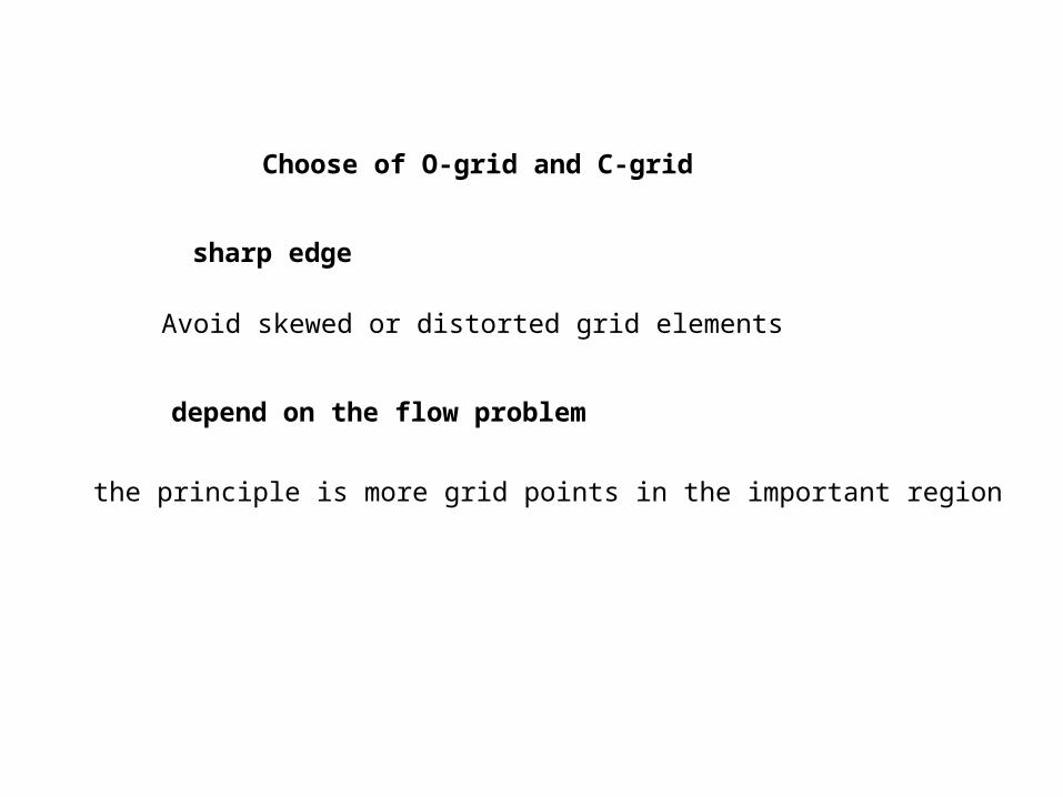
Example . Considering the Ux at point (i),

Ui+1=Ui+(Ux)i∆x1+0.5(Uxx)i(∆x1)2+

Ui-1= Ui(Ux)i∆x2+0.5(Uxx)i(∆x2)2+

1 12 1

2 1

( ) 0.5( ) ( )i ix i xx i

U UU U x x

x x

If ∆x2=∆x1 2nd order

If ∆x2 «∆x1

)xx()U(5.0 12ixx 1ixx x)U(5.0

1st order

1 12 1

2 1

( ) 0.5( ) ( )i ix i xx i

U UU U x x

x x

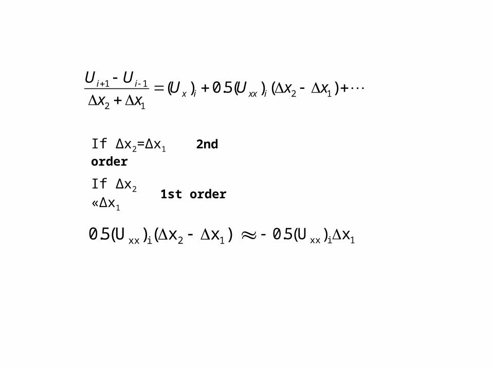
Grid generation---Possion equation method

Considering the solution of a steady heat conduction problem in 2D with Dirichlet B.C., the solution of this problem produces isotherms which are smooth and are nonintersecting. The number of isotherms in a given region can be increased by adding a source term. Hence, isotherms can be viewed as grid lines.

So we consider Poisson equations:

),( Pyyxx

),( Qyyxx

0)(2)( qxxxpxx

0)(2)( qyyypyy

22 yx yyxx 22

yx

/2PJp /2QJq yxyxyxJ

),(),(1

After the source terms p and q are specified with some methods on the boundary and interpolated into the inner domain， we can solve the equations，then the grid is obtained.

How to solve the above equations ?One solution: Five-point formula and GS.