78007

1

Final Research Report

Theoretical Model for Damage and Vibration Response inConcrete Bridges

(FRGS 78007)

Azlan Ab RahmanFaculty of Civil Enigneering

Universiti Teknologi Malaysia

Submitted to :

Research Management Centre (RMC)Universiti Teknologi Malaysia

August 2009

2

Theoretical Model for Damage and Vibration Response in Concrete Bridges(Keywords: vibration response, ambient testing, vibration signature, modal analysis)

Abstract

The use of vibration signatures for structural health monitoring (SHM) purposes has beenused in various fields, such as mechanical and aerospace engineering for many years. Inrecent years, its potential for use with civil engineering structures has been investigated andof particular interest in civil engineering is its applicability to buildings and bridges. It isrecently known that each structure has its typical dynamic behaviour, which may beaddressed as vibrational signature. Any changes in a structure, such as all kinds of damagesand deteriorations leading to decrease of the load-carrying capacity have an impact ondynamic response, hence suggesting the use of dynamic response characteristics for theevaluation of quality and structural integrity. Monitoring of the dynamic response ofstructures makes it possible to get very quick knowledge of the actual conditions and helps inplanning of rehabilitation budgets. One of the promising developments in structural vibrationmonitoring is the ambient vibration testing which does not require a controlled excitation ofthe structure. The structural response to ambient excitation can be recorded in large numberof points and from these ambient measurement, the condition of the structure can be derived.A classification of the structures can be developed based on vibration monitoring using themodal parameters natural frequencies, mode shapes, damping values and vibration intensities.The ambient vibration testing represents a real operating condition of the structure.

This report presents a theoretical and experimental ambient modal analysis on three existingstructures namely a staircase, a timber footbridge and a concrete bridge. The field-testing hasprovided opportunity to analyse dynamic properties of the three selected structures. Theoperational modal analysis software, ARTeMIS Extractor is a tool used for analysing the rawdata to obtain the dynamic properties of the structures. Finite element modelling and analysison the structure by using finite element software, ANSYS were developed. The comparisonbetween the mode shapes determined from both analyses showed some similarity. Thenatural frequencies that were generated had a variance between the two analyses. Thus, themodal updating is essential on the next stage. Improvement in the field-testing is needed inorder to obtain more accurate and quality results. Overall, modal analysis is comparable as analternative to extract dynamic properties of the structures.

Key Researchers:

Prof. Dr. Azlan Abdul Rahman (Head)Assoc. Prof. Baderul Hisham Ahmad

Mr. Ahmadon BakriYong Chou Yu (Civil Eng. B.Eng Student)

Faculty of Civil Engineering, Universiti Teknologi Malaysia

3

Model Teoritikal bagi Kerosakan dan Respon Getaran dalam Jambatan Konkrit

Penggunaan kaedah ‘tanda tangan’ getaran untuk tujuan penyeliaan keadaan kesejahteraanstruktur telah dibgunakan dalam pelbagai bidang seperti kejuruteraan mekanikal dan aero-angkasa sejak beberapa tahun dahulu. Kebelakangan ini, potensi penggunaan kaedah inidalam struktur kejuruteraan awam telah dikaji terutamanya applikasinya dalampenyelenggaraan dan penyeliaan bangunan dan jambatan. Adalah dikertahui bahawasesebuah struktur mempunyai kelakuan dinamik tertentu, yang boleh disifatkan sebagai‘tanda tangan getaran’. Sebarang perubahan di dalam struktur berkenaan, seperti pelbagaikerosakan dan keusangan yang mengakibatkan pengurangan keupayaan menanggung beban,akan memberi kesan ke atas respon dinamik. Oleh yang demikian, ianya mengisyaratkanbahawa ciri-ciri respon dinamik boleh digunakan untuk penilaian kualiti dan integritisesebuah struktur. Salah satu perkembangan yang berpotensi dalam bidang penyeliaangetaran struktur ialah teknik pengujian getaran sekitar yang tidak memerlukan penggegaranterkawal ke atas struktur yang diuji. Respon struktur terhadap getaran sekitar bolehdirekodkan dalam poin yang banyak dan maklumat keadaan struktur boleh diperolehi daripengukuran tersebut. Satu sistem klsifikasi juga boleh diwujudkan berdasarkan parametermodal gelombang semula jadi, bentuk modal, nilai penyusutan dan intensiti getaran.Pengujian getaran sekitar memberikan keadaan operasi sebenar sesebuah struktur.

Laporan ini menyampaikan analisis modal dengan getaran sekitar secara teori daneksperimen pada tiga struktur yang sedia ada iaitu sebuah struktur tangga, sebuah jambatankayu dan sebuah jambatan. Ujikaji di lapangan telah menyediakan peluang untukmenganalisis ciri-ciri dinamik tiga struktur yang terpilih. Perisian analisis getaran sekitar,ARTeMIS Extractor digunakan untuk menganalisis data bagi mendapatkan ciri-ciri dinamikstruktur tersebut. Model telah dibina dan dianalisis dengan menggunakan perisian kaedahunsur terhingga, ANSYS. Perbandingan dari kedua-dua analisis telah menunjukkan bahawaterdapat kesamaan dari segi bentuk modal. Terdapat perbezaan dalam frekuensi semula jadiyang dihasilkan dari kedua-dua analisis. Justeru, pengemaskinian modal adalah penting dandiperlukan untuk tahap yang seterusnya. Peningkatan prestasi pada ujian di lapangandiperlukan untuk mendapat keputusan yang lebih tepat dan berkualiti. Secara keseluruhannya,analisis modal merupakan suatu cara yang sesuai dan praktikal bagi mendapatkan ciri-ciridinamik struktur.

4

Acknowledgement

The author would like to thank his students, Mr. Yong Chou Yu and Teo Wei Heng for theirhardwork and commitment in carrying out the vibration measurement field-testing of threeselected structures. Special appreciation is due to Yong, who had helped to prepare the majorpart of the field-testing data analysis and report. Many thanks are also due to colleague andco-researcher, Assoc. Prof. Baderul Hisham Ahmad of Faculty of Civil Engineering, who hadsupervised the ambient vibration test on the selected structures and provided majorcontribution to the instrumentation technique for the testing activities. Technical assistancefrom Mr. Elfandy of Faculty of Mechanical Engineering during the field instrumentationwork is greatly appreciated.

5

Contents

INTRODUCTION

1.1 Introduction

1.2 Problem Statement

1.3 Objectives

1.4 Scope of Study

LITERATURE REVIEW

2.1 Introduction to Vibration

2.2 Basic Vibration Concept

2.2.1 Dynamic Loading

2.2.2 The Dynamic System

2.2.3 Equation of Motion

2.2.4 Modes of Vibration

2.3 Sources of Vibration

2.4 Modal Analysis

2.4.1 Function of Modal Analysis

2.4.2 Routes to Modal Analysis

2.4.3 Experimental Modal Analysis

2.4.4 Frequency Response Function

2.4.5 Frequency Response Function Model

2.4.6 Modal Testing Mechanism

2.4.6.1 The Excitation Mechanism

2.4.6.2 The Sensing Mechanism

2.4.6.3 The Data Acquisition and Processing Mechanism

2.4.7 Measurement of FRF Matrix

2.4.7.1 Single Input and Single Output Testing (SISO)

2.4.7.2 Single Input and Multiple Output Testing (SIMO)

2.4.7.3 Multiple Input Multiple Output Testing (MIMO)

2.4.8 Ambient Vibration analysis

2.4.9 Frequency Domain Decomposition (EDD)

2.4.10 Enhanced Frequency Domain Decomposition (EFDD)

6

2.5 ARTeMIS Extractor

2.5.1 Introduction

2.6 Finite Element

2.6.1 Introduction to Finite Element

2.6.2 History of Finite Element

2.6.3 Basic Steps in the Finite Element Method

2.6.3.1 Pre-processing Phase

2.6.3.2 Solution Phase

2.6.3.3 Post Processing Phase

2.7 ANSYS

2.7.1 Introduction to ANSYS

2.7.2 Overview of the ANSYS Program

FIELD TESTING AND ANALYSIS METHOD

3.1 General

3.2 Instrumentation Description

3.2.1 The Excitation Equipment

3.2.2 The Sensing Equipment

3.2.3 Data Acquisition and Processing Equipment

3.3 Small laboratory Testing

3.3.1 The Experimental Procedure

3.4 Ambient Modal Testing on Staircase

3.4.1 General Description of the Staircase

3.4.2 Staircase Testing procedures

3.5 Ambient Modal Testing on a Timber Footbridge

3.5.1 General Description of the Timber Footbridge

3.5.2 Timber Footbridge Testing Procedures

3.6 Ambient Modal Testing on a Concrete Bridge

3.6.1 General Description of the Concrete Bridge

3.6.2 Concrete Bridge Testing Procedures

3.7 Analysis using ARTeMIS Extractor

7

FINITE ELEMENT MODELLING

4.1 General

4.2 Finite Element Modelling of the Staircase

4.3 Finite Element Modelling of the Timber Footbridge

4.4 Finite Element Modelling of the Concrete Bridge

RESULTS AND ANALYSIS

5.1 Introduction

5.2 Ambient Vibration Data

5.2.1 Dynamic Characteristics of Tested Staircase

5.2.2 Dynamic Characteristics of Tested Timber Footbridge

5.2.3 Dynamic Characteristics of Tested Concrete Bridge

5.3 Finite Element Analysis using ANSYS

5.4 Comparison of Experimental Result and Finite Element Analysis

5.4.1 Required Instruments and Time Consumption

5.4.2 Accuracy and Subjectivity

CONCLUSIONS AND RECOMMENDATIONS

6.1 Conclusions

6.2 Recommendations

REFERENCES

APPENDICES A-D

8

1 Introduction

1.1 General Introduction

Vibrations or dynamic motions are naturally to life and regarded by mankind as unpleasantand unwanted phenomena causing undesirable consequences such as discomfort, noise,malfunctioning, fatigue, destruction and collapse. Structures being systems of elasticcomponents receive response, which subjected to dynamics and vibration analysis fromexternal and internal forces with finite deformations and overall motion. Natural disasterssuch as earthquakes are the most frightening manifestations of dynamic motion, which havelarge destructive impact on man-made structures (Nuno M. M. Maia and Julio M. M. Silva,1997).

Vibration is an element, which is hard to avoid in practice. Excitation of resonant frequenciesof some structural parts can occur with existence of vibration even it is only a smallinsignificant vibration. Then it can be amplified into major vibration and noise sources.Vibration can be easily defined as an oscillation which is the analogous to the motion of theparticles of a mass of air or the like, whose state of equilibrium has been disturbed. Itexhibited a movement first in one direction and then back again in the opposite direction. Thenumber of times that a complete motion takes place during the period of one second is calledfrequency which is measured in Hertz (Hz).

According to Bruel & Kjaer, oscillation normally varies with time and magnitude of aquantity refers to an indication, which may be greater or smaller than that indication.Basically random vibration is described by the three factors, which are amplitude, size andfrequency. Nowadays, vibration measurement and analysis on civil engineering structures hasbegun to gain popularity in civil engineering field. Technology developments have created anincreasing requirement for reliable dynamic analysis.

In civil engineering field, the behaviour of a structure at "resonance" is a key aspect ofstructural dynamic analysis. The natural frequency of vibration of a structure corresponds tothat structure's resonant frequency. Maximum displacements are produced if a structure issubjected to vibration at its natural frequency. The stresses, which developed in the framingmembers and connections of the structure, are greater when the displacements are increasing.For each mode, the structures will vibrate with a particular distorted shape called mode shape.After that the vibration dies out because of damping that removes energy from the structure.The interest of human’s ability to monitor a structure and detect damage at the earliest stageis persistent throughout the civil engineering communities. The damage detection methodsused are either visual or localized such as magnet field methods, acoustic and ultrasonicmethods, thermal field methods, radiography and eddy-currents methods. However most ofthese methods are subjected to limitations that require area of damage which known as apriori and is readily accessible. Only the damage near the surface can be detected throughthese methods (Charles R.Farrar and Scott W.Doebling, 1997).

Therefore there is a need to have a strong reliable vibration analysis tool to provideunderstanding of structural characteristics, operating condition and performance criteria thatenable designing optimal dynamic behaviour or solving structural dynamic problems inexisting designs (Nuno M. M. Maia and Julio M. M. Silva, 1997). Modal analysis is anapproach of knowing the natural frequency, mode shape and damping properties for a certain

9

structure. According to D.J Erwins, modal testing is the process involved in testingcomponents or structures with the purpose to obtain a mathematical description of theirdynamic or vibration behaviour. Indirectly it can provide the new knowledge and experienceof civil engineering, which can be used for future generic design. Most recently, developmentand verification of modal models have been of higher concern in today’s world. It is anapproach for structural modification based on modal analysis results.

There are mainly two types of structural dynamic testing namely forced vibration testing andambient vibration testing. The force method is conducted by dropping a known valued forceon the structure, which will induce a condition of free vibration. The ambient vibrationtesting represents a real operating condition of the structure, which uses the disturbances,induced by traffic and wind as natural or environmental excitations.

Modal analysis has become a major alternative to provide a helpful contribution inunderstanding control of many vibration phenomena, which encountered in practice.Determining the nature and extent of vibration response levels and verifying theoreticalmodels and prediction are both major objectives that can be achieved with experimentalmodal testing. Structures all over the world have become study subjects for the testing. Firstto emerge is the three spans, Z24 Bridge at Switzerland where a few of system identificationanalysis were performed to determine the dynamic characteristics of the bridge.

Repair and maintenance of infrastructure facilities are rapidly becoming a major financialburden for authorities bringing forth many new challenges for civil engineers. Key to thesuccessful upgrading of such structures is timely detection and quantification of damage anddeterioration, and in particular those, which builds-up over time during the functional life ofthe structure. The large stock of buildings and bridges, which are suffering from damage anddeterioration, would present a set of new challenges in the management of maintenanceissues. Factors such as improper design and construction without regard for maintainability orlife cycle costs, coupled with poor performance reliability and efficiency, would incur highfuture maintenance costs. This project attempts to identify the potential maintenanceproblems and maintenance management issues and propose a realistic long-term approach foreffective structural health monitoring. This research looks into the potential use of vibrationsignatures for structural health monitoring purposes which has been used in various fieldssuch as mechanical and aerospace engineering, in the assessment and monitoring of civilengineering structures. Of particular interest in civil engineering is the applicability ofdynamic response characteristics for the evaluation of quality and structural integrity ofbuildings and bridges. Monitoring of the dynamic response of these structures makes itpossible to get information of the actual conditions and helps in planning of rehabilitationbudgets. The research will look into the development of a structural classification system forcivil engineering structures, based on ambient vibration monitoring using modal parametersincluding natural frequencies, mode shapes, damping values and vibration intensities.

The proposed classification based upon vibration signatures would be useful in providing abaseline data and can be used to identify structures that show distinct problems and requireurgent maintenance and rehabilitation actions. Such classification system can be an effective

10

tool for assessment and priority ranking of the structures where a proposed budget planningcan be done according to the time schedule set up based upon the measured results of theambient vibration signatures.

Basically structural evaluation is based almost entirely on visual inspection, which is limitedby accessibility and subjectivity. It is normally carried out when there is a segment of thestructure suspected to be defective. Structures assessment in health monitoring also can becarried out based on the modal properties obtained from the structures. Besides that, most ofthe structures in Malaysia are designed based on static load approach without considerationof vibration on the structure during the design stage. Vibration design is under considerationmostly in the high rise building design only. Malaysia is not located in the earthquake andtyphoon zone but the incidents that happen lately such as Tsunami and earthquake in SouthEast Asia region had a slightly impact on Malaysia. Some parts of Malaysia can feel thevibration of the earthquake when it happened outside of Malaysia.

Modal analysis is a solution to obtain the actual structural dynamic properties. The dynamicproperties, which consist of natural frequency, mode shape and damping, are unknown on thedesign. The frequencies of vibration of the structure are directly related to the stiffness andthe mass of structure while the mode shapes are related to the defect location. Thereforevibration testing needs to be carried out to obtain the data of those dynamic properties forstructural health monitoring and evaluation.

Civil engineering structures normally are in large size so it is viable to get excitation fromambient vibration method. Ambient testing is chosen for this study due to its importance inrepresenting the real operating condition that could be related to normal excitation or naturaldisaster especially impact of excessive wind load on structure. Since ambient testing does notinterrupt service of the test structure, it can be conveniently applied for long term healthmonitoring of structures.

1.2 Problem Statement

Recent issues on problems in structural integrity of buildings and bridges in Malaysia hashighlighted the challenges faced by the authorities who need effective methods in structuralpriority ranking concerning maintenance, rehabilitation planning and structural monitoringactions. Buidling or infrastructure owners and authorities, who need to manage a large stockof structures will face challenges when structural performance falls short of “excellent”because the serviceability and economic impacts are too severe to accept. Owners ofbuildings and other civil infrastructure require effective methods in structural priority rankingconcerning actions on maintenance, rehabilitation planning and lifetime assessment. Withlimited maintenance budgets, managers and owners require priority-ranking tool in decisionmaking to link between optimized use of budget and effective maintenance activities.

The use of vibration signatures for structural health monitoring (SHM) purposes has beendeployed in various fields, such as mechanical and aerospace engineering for many years. Inrecent years, its potential for use with civil engineering structures has been investigated andof particular interest in civil engineering is its applicability to buildings and bridges. It is

11

recently known that each structure has its typical dynamic behaviour, which may beaddressed as vibrational signature. Any changes in a structure, such as all kinds of damagesand deteriorations leading to decrease of the load-carrying capacity have an impact ondynamic response, hence suggesting the use of dynamic response characteristics for theevaluation of quality and structural integrity. Monitoring of the dynamic response ofstructures makes it possible to get very quick knowledge of the actual conditions and helps inplanning of rehabilitation budgets.

One of the promising developments in structural vibration monitoring is the ambientvibration testing which does not require a controlled excitation of the structure. The structuralresponse to ambient excitation can be recorded in large number of points and from theseambient measurement, the condition of the structure can be derived. A classification of thestructures can be developed based on vibration monitoring using the modal parametersnatural frequencies, mode shapes, damping values and vibration intensities. The proposedclassification can be used to identify structures, which show distinct problems and urgentlyrequire maintenance and rehabilitation actions. A proper budget planning of the responsibleauthority can be done according to the time schedule set up based upon the measured resultsof the ambient vibration system. Such classification can be a very effective tool forassessment and priority ranking of the structures.

1.3 Objectives

The purpose of this research is to study the dynamic properties and behaviour of selectedstructures by using ambient modal analysis and compare with the finite element analysis.Objectives of this research are as follow:

a) Iddeennttiiffyy tthhee ppaarraammeetteerrss aanndd ccrriitteerriiaa ffoorr ddeetteerrmmiinniinngg vviibbrraattiioonn ssiiggnnaattuurree ooff bbrriiddggeessttrruuccttuurreess

b) Obtain the experimental dynamic properties, which consist of natural frequency,mode shape and damping ratio of selected structures using operational modalanalysis.

c) DDeevveelloopp aa tthheeoorreettiiccaall ffiinniittee eelleemmeenntt mmooddeell ffoorr ccoorrrreellaattiinngg tthhee sseevveerriittyy ooff ddaammaaggeeaanndd tthhee cchhaannggee iinn rreessoonnaanntt ffrreeqquueennccyy aanndd ddaammppiinngg ooff sseelleecctteedd ssttrruuccttuurreess..

d) Perform modal analysis of the selected structures to obtain the theoretical dynamicproperties, which consist of natural frequency and mode shape.

e) Compare measured results from ambient vibration analysis of the tested structureswith the finite element analysis of the structures.

1.4 Scope of Study

The scope of research that needs to be carried out consists of two parts, which are theoreticalpart and experimental vibration testing. First part is the experimental modal analysis onselected structures and the analysis are done using software called ARTeMIS Extractor. Theambient experimental testing is conducted using natural sources and hammer approach as

12

artificial impact. A trial experimental testing is conducted on the first stage of experimentaltesting. The small laboratory trial experimental testing on a plate is conducted at theVibration Laboratory.

Three structures in Universiti Teknologi Malaysia (UTM) are selected to conduct modalanalysis as follows:

1. Preliminary vibration test on a staircase structure2. Vibration test on a timber footbridge.3. Full-scale vibration test on a concrete bridge.

It is followed by the second part, which is theoretical part, involving the use of finitemodelling. ANSYS software is used in the modelling and analysis for the selected structures.The results from the analysis in ANSYS will be the theoretical dynamic properties of thestructures. Lastly, comparison is made between the experimental results and the finiteelement analysis to extract similar dynamic properties of the tested structures.

13

2 Literature Review

2.1 Introduction to Vibration

In Civil Engineering field, vibration has become a big concern for civil engineers nowadaysin their design. Before that, civil engineers pay more attention to static analysis in theirdesign but some incidents happen where one of the famous oscillation incidents was the greatTacoma Narrow Bridge in Washington State. A steady wind led the bridge to ultimatedestruction of this fine structure only few months after the completion. It became the objectof scrutiny for structural engineer and none of them want to repeat the costly mistake infuture.

Vibrations or oscillations can be regarded as a solution of dynamics in which when subjectedto internal or external restoring forces either due to elasticity or gravity, a system swing backand forth about an equilibrium position and is defined as an assemblage of parts actingtogether as a whole. There is one dangerous phenomenon where the loading imposed on thestructure would create a periodicity that synchronises with the natural frequency of thestructure (J.R Maguire and T.A. Wyatt, 1999). In another word, the force will cause aperceptible motion if the frequency of application is well below the vibrating structure’sfrequency that can oscillate freely with distortion on its own (R.E.D Bishop, 1979). Thismagnification is known as resonance, which will create exaggeration of response withpotential fatigue failure that needs to be avoided in civil engineering.

2.2 Basic Concepts

2.2.1 Dynamic Loading

Based on the nature of the time-wise variation, dynamic loading can be categorized into fourtypes, which are (J.R Maguire and T.A. Wyatt, 1999):

a. Harmonic or periodic.It is also known as a steady state loading which frequency and amplitude play the majorrole and time playing for a secondary role only. The loading consist forces that simplyproportional to the trigonometric function of sin ωt or cos ωt or a combination of both.Amplitude of this load type repeats itself many times in a regular basis. The commoncharacteristic of the function from the loading is its values can be determined for anyfuture time t, which is called deterministic. Machinery loading is the example ofharmonic loading.

b. Transient.Initial excitation is referred to at times as transient excitation where all motions caused byinitial excitations come to rest eventually. Transient loading varies with time so it doesnot repeat itself continuously. It is exactly contrast with harmonic loading. Blast loadingis one of the examples in this category.

c. Stationary random.This type of loading is in the category where the phenomena of the outcome at a futureinstant of time cannot be predicted. Although the value of the load cannot be determined

14

precisely, the statistical properties of the loading vary in a gradual manner such as windloading that varies in velocity so as the excitation imposed.

d. Non-stationary random.It is actually the same as stationary random but the difference is the statistical propertiesvary only swiftly. Earthquake loading is categorized in this type of loading becauseearthquake frequently happens in a flash of time.

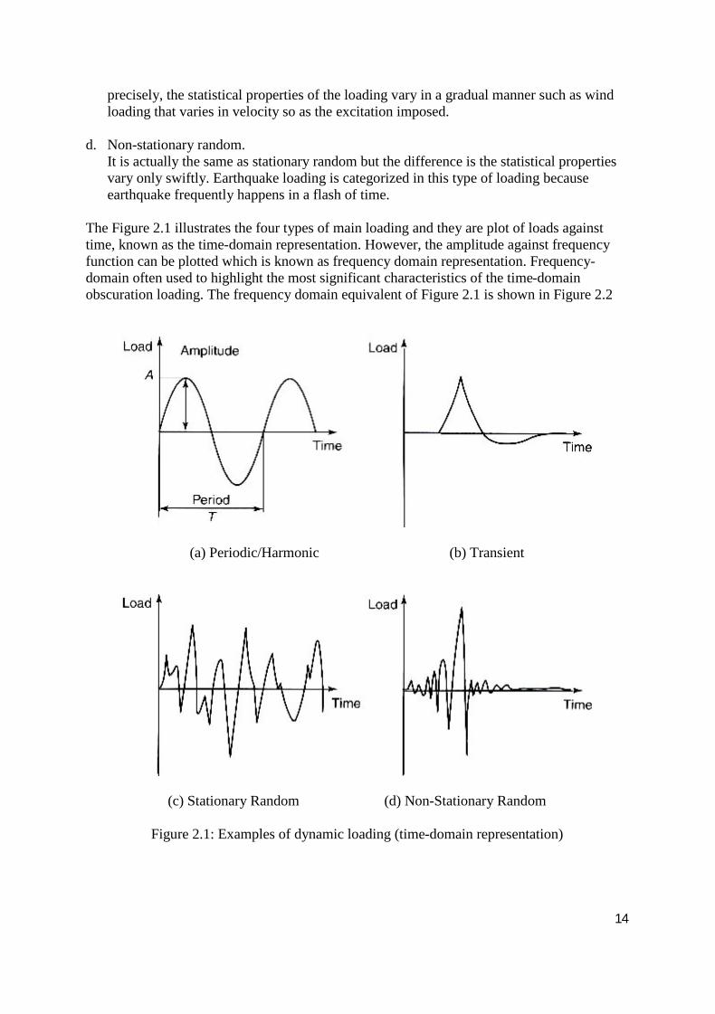
The Figure 2.1 illustrates the four types of main loading and they are plot of loads againsttime, known as the time-domain representation. However, the amplitude against frequencyfunction can be plotted which is known as frequency domain representation. Frequency-domain often used to highlight the most significant characteristics of the time-domainobscuration loading. The frequency domain equivalent of Figure 2.1 is shown in Figure 2.2

(a) Periodic/Harmonic (b) Transient

(c) Stationary Random (d) Non-Stationary Random

Figure 2.1: Examples of dynamic loading (time-domain representation)

15

Figure 2.2: The frequency-domain equivalent

2.2.2 The Dynamic System

The dynamic system in civil engineering field can be divided according to their behaviourinto two major types. Implication of the principle of superposition is usually valid in civilengineering structure and it is called linear system. However, the principle of superpositionthat linear system holds cannot be applied on the nonlinear system. The distinction betweenlinear and non-linear systems frequently depends on the range of operation but not inherentproperty of the system. Although there are many approaches to study non-linear system,qualitative and quantitative approaches are most commonly used.

Linear analysis is more familiar in dynamic because it is to assist evaluation by modalanalysis. Another reason that linear analysis remains common is that it is suitable for manydynamic criteria such as fatigue and comfort, and the dynamic response is mostly within thelimit. Therefore, any system must have certain characteristics before it will vibrate. In firstNewton’s Law, it will stay in the equilibrium position and will tries to return to the stableposition if it is disturbed. The restoring force is called stiffness force, which is proportional tothe displacement of the structure while the coefficient of proportionality is called the stiffnessof the structure. The stiffness possesses potential energy or strain energy within the structure.Requirement to overshoot its equilibrium position is the structural must also own mass togenerate vibration.

After the certain period, the motion starts to slow down and stop after awhile.In this case, the system is said to be ‘damped’. Some energy dissipating mechanism is behindthis phenomenon. The damping will cause the amplitude of the displacements to fade withtime if there is no additional energy input. An ideal assumption is made where the dampingforce is proportional to the velocity of the structure. In conclusion, a common idealization isto assume that the damping is vicious.

2.2.3 Equation of Motion

Basically, the inertia force, damping force and stiffness force together with externally appliedforce will form the equation of equilibrium between them, which is called the ‘equation ofmotion’ that defines the dynamic behaviour of the structure.It is in the form of:

16

Inertia force + damping force + stiffness force = external force

When in algebraic form, the equation becomes: mÿ + cý + ky = f (t)

The equation of motion controls almost any structure’s linear dynamic behaviour and thedynamic response can be found by solving this equation of motion. Values at the selectedlocation, the degrees of freedom (DOF) will embody the displacement in a structure. Figure2.3 shows the example of single DOF system. The reason it is chosen because an accurateestimation of the kinetic energy can be made. The equation is form in matrix form where thestiffness is called K, the mass matrix is called M and the damping matrix is called C and theequation is:

Mÿ + Cy + Ky = F

Figure 2.3: Example of single DOF system

2.2.4 Modes of Vibration

Every structure does not necessary has only single degree of freedom (DOF) but the systemwill have numbers degree of freedom and thus it will have numbers of solution indicating themodes of vibration of the system. A free vibration exists in each mode with certain frequencyand certain mode shape.

The normal modes are independent of each other where they do not affect each other’s mode.The problem can be solved by using the simple degree of freedom solution’ to obtain thesuperposition of the modal response. This is where the modal analysis plays its extremelypowerful part and adopted almost universally.

2.3 Sources of Vibration

Vibration and shock can arise from a variety of sources, which may be generated from naturalsources and also possibly from human activities. They may produce annoyance anddiscomfort. Some of them even involve structural damage when severe conditions occur andthe extensive damages may cause disasters that are beyond our imagination. The typicalsources of vibration either natural or excitations from human activities are:

17

a. Road vehiclesb. Earthquakesc. Aircraftd. Machinery and industrial plante. Forging hammers and drop-stampsf. Pile drivingg. Windh. Hydrodynamic loadingi. Blasting

Civil engineer should not overlook on the vibration that occur on a structural that may turninto unstoppable disaster. Therefore as a civil engineer, one should be able to determine thesources of vibration and encounter them in the structural design.

2.4 Modal Analysis

Structural health monitoring is pervasive in civil engineering because it is an analysis of thedynamic behaviour of civil structures to observe and examine the integrity of those structures.It involves different parameter and damage identification. Visual inspection is limited by theinability to classify invisible damage, which only can detect the damage near the surface.However, modal analysis fulfils the requirements of global in nature and automated thatexamine changes in the vibration characteristics of the structure (Ayman Khalil, Lowell.G,Terry J.W and Douglas W., 1998).

Modal analysis was first applied around 1940 as an engineering tool in the search for betterunderstanding of aircraft dynamic behaviour. However, it did not see extensive developmentin scientific and engineering until availability of the invention of smaller, faster computer andboosting in signal analysis with the introduction of signal processing algorithm such as FastFourier Transform (FFT) spectrum analysers (Nuno M. M. Maia and hulio M. M. Silva.1997). Modal testing become a mature technology in the 1980s and advanced to feature inmechanical and aerospace Master of Science and undergraduate curricular at universities inEurope and North America. Although modal testing was developing in 1990s, it stillremained unfamiliar research topic in civil structural engineering. Then finite element modelupdating based on modal testing results was under great development in 1990s (AleksandarPavic 1999). Today, modal analyses are used on large engineering structures, which aresubjected to dynamic motions or vibrations.

It is well known that structures can resonate where the small forces can result in importantdeformation and damage can be induced in the structure. For an example, a bridge disasterwhere the Tacoma Narrows suspension bridge collapsed due to wind-induced vibration onNovember 7, 1940. The bridge was only opened for traffic just a few months before itcollapsed. In addition, most of the structures can be made to resonate. Interaction between theinertial and elastic properties of the materials within a structure contributes to resonantvibration. Identification and quantification of resonant frequencies of a structure is needed toobtain better understanding of any structural vibration problem. That is the reason why todaymodal analysis is developed and used to access structural dynamic behaviour of certainstructures (Patrick Guillaume, 2002).

18

2.4.1 Function of Modal Analysis

The main function of modal analysis is the process to describe the dynamic behaviour of astructure from test data construction to a mathematical model. According to Nuno M. andJulio M., a set of accurate and sufficiently extensive in both the frequency and spatial domainFrequency Function (FRFs) are able to acquire from this form of vibration testing. Then,analysis and extraction of the properties for all the required modes of the structure can bedone from the FRFs (Nuno M. M. Maia and hulio M. M. Silva, 1997). Natural frequencies,mode shapes and modal damping ratios are the measurement and estimation of a structure’smodal properties. They serve as parameters that detect and locate possible damage ofstructures, long-term health monitoring of structures, basis input to the finite element modelupdating and evaluation of structures against different harsh situation such as wind load andearthquake.

Modal analysis is capable of extracting the modal natural of the structures from themeasurement made on the vibrating structures with a range of analysis procedures. Theindependence of modal properties serve as the basis of a mathematical model of the samestructure which leads to the same modal properties starting not from data that measured, butfrom the mass, damping and stiffness distribution that assumed in the structure (AleksandarPavic 1999).

The capabilities of the transducer and data processing equipment will affect frequencydomain extent of the model during the testing while the experimental setup will influence theaccuracy and correctness of the model. There will be unwanted modification effect on thestructure for almost all the methods of applying as well as unwanted influence from almostall the response measurement transducers and support fixture on the structure. Awarenessshould be taken care to select the appropriate method of excitation and response measurementfor obtaining the accurate and reliable results (Nuno M. M. Maia and hulio M. M. Silva.1997).

2.4.2 Routes to Modal Analysis

Modal analysis can be carry out in experimental and theoretical. There are three key modelsthat can be used to illustrate dynamics of a vibrating structure, which are:

1. The modal modelThe structure’s dynamic properties are represented in terms of natural frequencies, modeshapes and modal damping ratios.

2. The spatial modelThe structure’s dynamic properties are represented in terms of its mass, stiffness and dampingproperties

3. The modal modelThe model represents the structure’s dynamic properties in terms of series of transferfunctions, usually the Frequency Response Functions (FRFs).

19

2.4.3 Experimental Modal Analysis

Experimental modal analysis is the process that applies experimental approach to determinethe modal parameters of a linear, time invariant system. The modal parameters describe mostof the vibration and acoustic problems for both the functions and the system characteristics.There are several simple and short phases involve in the process of determining modalparameters. The process of determining modal parameters from experimental data involvesseveral phases. Specific goals in terms of reducing the errors associate with that phase willdetermine the success of the experimental modal analysis. The possible delineation of thephases are:

a) Modal Analysis Theoryb) Experimental Modal Analysis Methodsc) Modal Data Acquisitiond) Modal Parameter Estimatione) Modal Data Presentation/Validation

Assumptions concerning any structure are made in order to perform an experimental modalanalysis. However, these basic assumptions are only approximately true and they can beevaluated experimentally during the test and after performing the data analysis. The validityof the assumptions involved in modal analysis need to be measured before conducting thetesting. The basic five assumptions that usually made are:

1. The structure is assumed to be linearThe structure obeys the principle of superposition where the response of the structure to anycombination of forces that applied simultaneously is the sum of the individual responses toeach of the forces acting alone. A controlled excitation experiment that apply the forcesapplied to the structure with a form convenient for measurement and parameter estimationwhich relatively almost similar to the forces that act naturally to the structure in its normalenvironment can characterise the structure’s behaviour.

2. The structure is time invariantTime invariant means that the parameters that are to be determined are constants throughoutthe testing. Components such as mass, stiffness, or damping on a system, which is not timeinvariant generally depend on factors that are not measured or are not included in the model.

3. The structure obeys Maxwell’s reciprocityIt means that the frequency response function between a point called p and another pointcalled q is the same when the response on a point called p when force is excited on a pointcalled q compared with the measured response at q when a force applied at p (Hpq Hqp).Another explanation for reciprocity is that the degree-of-freedom p causes a response atdegree-of-freedom q that is the same as the response at degree-of-freedom p caused by thesame force applied at degree-of freedom q.

4. The structure is observableAdequate behavioural model of the structure can be generated with sufficient informationfrom the input-output measurements. Structures are not complete observable due to the loosecomponents or degrees-of freedom of motion that are not measured. This occurs in at leasttwo different ways. The first way is the limitation of data to a minimum and maximum

20

frequency and limited frequency resolution. Secondly, the information relative to localrotations is not available because lack of transducers available in this area.

5. The structure is causal and stableThe system is in rest mode before it is excited if the structure is causal while the structure isstable because the vibrations will cease after the excitation is removed.

2.4.4 Frequency Response Function

Frequency Response Function (FRF) consists of real and imaginary components and it acts asa complex transfer function, which expressed in the frequency domain. It may also berepresented in terms of magnitude and phase where the response parameter may appear indenominator or numerator of the transfer function. It displays the independent of theexcitation function characteristic where the excitation could be random, periodic or transientfunction of time. Furthermore measured data or analytical functions form a frequencyfunction expresses the structural response as a function of frequency in terms ofdisplacement, velocity, or acceleration from the result obtained with one type of excitationthat can be used to predict the response of the structure to any other type of excitation (T.Irvine 1999).

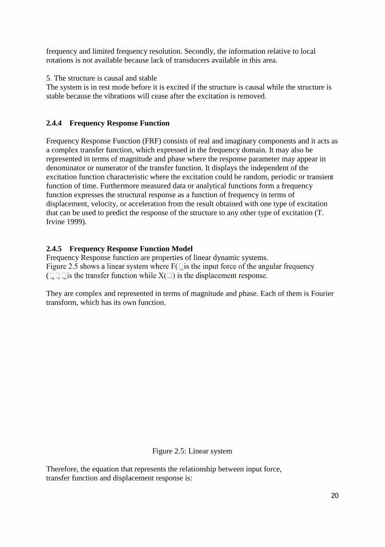
2.4.5 Frequency Response Function ModelFrequency Response function are properties of linear dynamic systems.Figure 2.5 shows a linear system where F((

They are complex and represented in terms of magnitude and phase. Each of them is Fouriertransform, which has its own function.

Figure 2.5: Linear system

Therefore, the equation that represents the relationship between input force,transfer function and displacement response is:

21

2.4.6 Modal Testing MechanismThere is a variety of hardware component available for modal testing but there are mainmeasurement mechanisms which are:

1. The excitation mechanism2. The sensing mechanism3. The data acquisition and processing mechanism

2.4.6.1 The Excitation MechanismIn the excitation mechanism, the input under the form of driving force is applied at a givencoordinate of the structure under analysis (Nuno M. M. Maia and Hulio M. M. Silva. 1997).There are two types of techniques generally used for modal test excitation which are impulseor impact hammer excitation and shaker excitation.

The first of these involves either out of contact throughout the vibration or only applied incontact for a short period. The second type includes an exciter which remains attached to thestructure throughout the test with continuous or transient excitation (D.J Erwins, 1985). Eachof the technique has their own features, advantages and disadvantages but data collected fromboth techniques is exactly the same from a theoretical standpoint. Difference between thedata from practical point is caused by factors such as the structure suspension, the mass of themounted transducer and stiffening effects of the shaker arrangement (Pete Avitable 1998).Impulse or impact hammer is simply a hammer with a force transducer attached to its head todetermine component or system response to impacts of varying amplitude and duration bypairing with an accelerometer or more on the component being tested. It does not need asignal generator and power amplifies.

Force, pulse duration and frequency range are the most critical specifications for impulsehammer in modal testing. Hammer mass and hardness of its impacting head contribute to thedifference of the range of frequency. Besides that, the amplitude of impact force is affectedby the mass together with the velocity of impaction (Nuno M.M. Maia and hulio M. M. Silva. 1997). It is the most commonly used technique that exciteswide range of frequency in modal testing. Impulse hammer excitation is chosen because ofthe inexpensive cost, quick and easiness to perform the modal testing. However, sometimesthe input force can be different from measurement to measurement which caused by lack ofcontrol over the frequency content of the excitation and poor signal ratio (Pete Avitable1998). Figure 2.6 shows the hammer that induced force in modal testing.

22

Figure 2.6: Impulse hammer used in modal testing

Shaker excitation is mostly used in more complex structure with vibration provided by forcegenerators or transducers. “Shaker is usually an electromagnetic or Electro-hydraulic vibratordriven by power amplifier (Nuno M. M. Maia and Hulio M. M. Silva. 1997). Themeasurement for shaker excitation is serial or parallel measurements. There are many typesof excitation technique in shaker excitation and two that broadly used are steady stateexcitation and broadband excitation (P. Reynolds and A. Pavic 2000). Both frequency andamplitude can be easily controlled so it offers accurate result (Nuno M. M. Maia and HulioM. M. Silva. 1997). Shaker excitation is suitable to use in repeatable experiment compare toimpulse hammer excitation. It can be used for MIMO analysis, which has many inputs andoutputs where data collected will be more accurate to produce good results. This technique isnot widely used because of the difficult setup process and skill operators are needed to usethe shaker excitation. It involves more equipment and channel that make it more costly to usein modal testing (P. Reynolds and A. Pavic 2000). Figure 2.7 shows the one of the exampleof shaker used in modal testing.

Figure 2.7: Shaker used in modal testing

2.4.6.2 The Sensing MechanismBasically, the sensing mechanism is constituted by sensing devices and conditioningamplifiers. Various sensing devices known as transducer are available in modal testing butpiezoelectric transducers are usually used in experimental modal analysis. They are able todetermine force excitation, which called forced transducers and determining response which

23

called accelerometers. Purpose of transducers is generation of electric signals that areproportional to the physical parameter which one wants to measure. Conditioning amplifierserve the purpose to solve the problem of weak signals generated and electric impedancemismatched (Nuno M. M. Maia and Hulio M. M. Silva. 1997). The examples ofaccelerometer are shown in Figure2.8.

Figure 2.8: Examples of accelerometer

2.4.6.3 The Data Acquisition and Processing MechanismThe complicated devices known as analysers basically are used in data acquisition andprocessing mechanism to determine development of signals by the sensing mechanism and toascertain the magnitude and phases of the excitation forces and responses. The common usedanalysers which called Spectrum Analysers of FFT Analysers are based on the Fast FourierTransform (FFT) algorithm and provide direct measurement of the FRFs. Transducersgenerate the analogue time domain signals that will be converted into digital frequencydomain information that can be processed with digital computer are done by the analysers. Inother words, analysers received measurements of time varying excitation forces applied to thestructure and corresponding dynamic acceleration responses to compute FRF accelerancedata for a selected structure (Nuno M. M. Maia and hulio M. M. Silva. 1997). Figure 2.9shows the signal analyser used in modal testing.

Figure 2.9: Signal Analyser in modal testing

24

2.4.7 Measurement of FRF Matrix

2.4.7.1 Single Input and Single Output Testing (SISO)The SISO testing is conducted using one roving excitation and one accelerometer attached toa single DOF as the fix reference of the structure. The fix reference then receives excitationsequentially from the hammer. Reference DOF needs to be selected carefully because itcontains information about all the mode shapes in the interested frequency range. Thereference in a nodal position for any mode should be prohibited from selection because thenode of mode is a location of zero response (Pete Avitabile 2002).

2.4.7.2 Single Input and Multiple Outputs Testing (SIMO)There is another alternative for modal testing that is multiple references testing where two ormore response accelerometers are fixed to the two or multiple references. Then, one rovingexciting is performed. Tri-axial accelerometer is often used to capture movements in alldirections simultaneously. This testing is used when single reference DOF which contain allmode of interest is impossible to find and multiple references are required. Anotheradvantage of SIMO testing over SISO testing is it can detect repeated roots.

2.4.7.3 Multiple Input Multiple Outputs Testing (MIMO)The structure is excited at two or more DOFs and the output is measured in two or moreresponse DOFs. MIMO testing is usually conducted on complex structure, which have localmode that the reference DOF with modal deflection for all modes is not available. Themultiple outputs are measured on the same time to give consistent data. Furthermore theMIMO testing has the following advantages:

a) Distribution of sufficient energy over the complete structure.Sufficient energy is needed to distribute over the structure, which is large and heavilydamped.

b) Avoidance of non-linear behaviour.Distributing the energy over the structure using multi-point excitation reduces theforce level at the different excitation DOFs thereby avoiding driving the structure intonon-linear behaviour that would deteriorate the estimation of the FRFs.

c) Better simulation of real-life operationMIMO testing provides a better representation of the excitation forces that load thestructure during real-life operation.

d) Reduced force drop-offs at resonance frequenciesMultiple smaller shakers will lead to smaller drop-offs at resonance frequencies.

e) Reduced test timeMIMO testing consumed less time on-structure by using multiple shakers andmultiple references.

2.4.8 Ambient Vibration analysisAmbient vibration analysis is when the modal properties are only identified from measuredresponse. It can be called “output only identification” or “operational modal identification”because only response data are measured but the actual loading conditions are unknown. The

25

terms “ambient identification” or “ambient response analysis” are often used. Besides that, itdoes not directly lend itself to FRFs calculations because the input forces are not measured.The main purpose of ambient vibration analysis is to determine the modal parameters fromexperimental data. The modal parameters are mode shapes which the way the structure movesat a certain resonance frequency, natural frequencies that represent the resonance frequenciesand damping ratios which the degree to which the structure itself is able of damping outvibrations.

Excitation on large civil engineering structures by natural loads are often not easilycontrolled, for instance wind loads on building, wave loads on offshore structures, or trafficloads on bridges. Thus, it is an advantage to use output-only modal identification. The naturalexcitation is used as the excitation source instead of artificially exciting the structure anddealing with the natural excitation as an unwanted noise source.

Ambient vibration testing is generally preferred to non-destructive forced vibrationmeasurement techniques for obtaining the modal parameters of large structures for manyreasons. A structure can be adequately excited by wind, traffic, and human activities and theresulting motions can be readily measured with highly sensitive instruments. Consequently,the overall cost of the measurements conducted on a large structure is reduced (Ventura, C.E.and Horyna, T, 2000). There have been several output-only data modal parameteridentification techniques available that were developed by different investigators for differentuses such as: peak picking from the power spectroutput only modal parameter ideal densitiesauto regressive-moving average (ARMA) model based on discrete-time data naturalexcitation technique Output-only modal parameter identification of civil engineeringstructures 3 (NExT), and stochastic subspace identification (X.He, B.Moaveni, J.P.Conte andA.Elgamal, 2003). The advantages of the operational modal testing are:

Testing is cheap and fast because excitation equipment is not needed.Therefore, the physical setup is very straightforward and fast.

There are difficulties or impossibilities to test the structures by forces.Artificial inputs cannot be applied to a structure or they cannot be measured correctlydue to the structure's boundary conditions or physical size thereby making classicalmodal analysis impractical. Special boundary conditions are not needed for the testingand it is in-situ testing (Proefschrift, 2005).

Measurements are done in the actual operation conditions for the structure but they donot interfere with the operation of the structure. Identified modal parameters representthe dynamic behaviour of the structure in reality.

There are also some disadvantages of conducting the modal operational testing which are:

a) The modal model used is not up to scale.b) An assumption is made that excitation cover interested frequency range.c) The calculation and computation is complicated and intensive which lead to time

consuming.d) Sensitive equipment is needed

26

2.4.9 Frequency Domain Decomposition

Frequency Domain Decomposition (FDD) is implemented by Brinker, Zhang and Andersen(2000), as well as Shih (1989), who used Singular Value Decomposition for each frequencyline of the response spectral density matrix, known as non-parametric technique. Singlevalues are inferred as a combination of auto-power spectra for a set of Single-Degree-Of-Freedom (SDOF) systems. It can identify the natural frequency and mode shape at aparticular peak of each of the SDOF systems. The FDD technique provides the physics of thestructure system by peak-picking method technique. It involves conversion of output signalsinto frequency response function by means of the Fourier Transform. It is a simple techniquethat starts by identifying the SDOF function after looking at the plot and then picks the peakof the function for each resonance on the average of the normalized singular values. Theinformation extracted from singular values is just one single frequency line. The naturalfrequency corresponds to the peaks of these response plots. Mode shapes are outcome fromcorrelation of the phase angle information with the peak magnitude (Troy M.Dye, 2002).Thus, good results of natural frequencies and mode shapes can be determined but notdamping estimation.

2.4.10 Enhanced Frequency Domain Decomposition

The Enhanced Frequency Domain Decomposition (EFDD) is extension techniques of theFDD that can be used to obtain damping as well as natural frequencies and mode shapes.Dynamic characteristics of particular mode are extracted from the corresponding SDOFnormalized auto-correlation functions in the time domain. FDD and EFDD is a fast, easy touse and accurate peak picking techniques in modal analysis.

2.5 ARTeMIS Extractor

ARTeMIS Extractor is software that is used to analyse ambient vibration data to determinethe modal parameters which are natural frequency, mode shape and damping ratio. ARTeMISExtractor is effective in modal identification from response only and identification ofstructure under real operating condition.

ARTeMIS Extractor supports three ways to create project by entering three types ofinformation:1. SVS Configuration File definition.2. Universal File Format.3. OLE Automation.

Universal File Format is used in the modal analysis that is conducted in this research study.Universal file format can be defined as data that stored in a data set which called UFF thathas different numbers. There are four types of data set that are necessary to create a project inARTeMIS Extractor which are:

1. UFF Data Set Number 15The data sets contain the node definition which equal to the group in the SVS ConfigurationFile format that starts with the keyword “Nodes”. It is actually the coordinates of the pointthat form the structures.

27

2. UFF Data Sets Number 82This data set is to create the line of the geometry. They are optional data sets which containtrace line definitions and equal to the group in the SVS Configuration File format that startswith the keyword “Lines”

3. A UFF Data Set Number 2412They are other optional data sets which have triangular surface definitions and equal to thegroup in the SVS Configuration File format that starts with the keyword “Surfaces”. They areused to create the surface of the structures in geometry modelling.

4. UFF Data Sets Number 58A specific node in a specific direction is contained inside these data sets and equal to thegroup in the SVS Configuration File format that starts with the keyword “Setup”. They arethe raw data file recorded by data acquisition system during experimental testing.

2.6 The Finite Element

2.6.1 Introduction to Finite Element

Finite element is a numerical technique used to obtain approximate solutions of boundaryvalue problems in engineering. Boundary value problem is a mathematical problem in whichone or more dependant variables must satisfy a differential equation everywhere within aknown domain of independent variables and satisfy specific conditions on the boundary ofthe domain (David V.Hutton, 2004). They are used when hand calculations cannot provideaccurate results.

In the finite element analysis of real structures, the actual structure is broken down into manysmall pieces of various types, shapes and sizes which then assembled together using the basicrules of structural mechanics, equilibrium of forces and continuity of displacements. Theysolve the field with discrete model. The field variables may include temperature, vibration,displacement and others.

Finite element has become a vital tool for students and engineers to solve various types ofproblems and unknown.

2.6.2 Basic Steps in the Finite Element Method

The finite element method (FEM) can be defined as a general numerical technique forapproximating the behaviour of continua by assembly of small parts (elements). In finiteelement modelling, discretize the continuous structures that have infinite numbers of degreeof freedoms into smaller pieces called elements for analysis is an important process. Afterthat, stiffness is determined and assembled into the system of equilibrium equation to solvenodal displacements. Different properties and geometries will be required to cater for varioustypes of structures and their behaviours. The procedures involved in finite element analysisconsist preprocessing phase, solution phase and post processing phase (T.R. Chandrupatla &A.D. Belegundu, 1997).

28

2.6.2.1 Pre-processing PhaseGeometric domain of the problem is defined. The solution domain is created and discretizedinto finite elements by subdividing the problem into nodes and elements depending onengineering judgement. It is either small enough to give accurate result or large enough to letthe computational process easier. It is assumed that a shape function depends on the physicalbehaviour of an element and approximation of the simulation of the actual behaviour of theproblem. Equations then develop by defining the material properties, geometric properties,element connectivity as well as the boundary condition (physical constraints) and the loading.The global stiffness matrix will be constructed after assembly of the elements that representthe entire problem.

2.6.2.2 Solution PhaseA set of linear or non-linear algebraic equations will be solved simultaneously. The solutionwill give the nodal results for example displacement values at different nodes. Reduction ofdata storage requirements and computation time will be achieved by this solution technique.Gauss elimination is commonly used for static and linear problems. Additional computationand variables derivation such as reaction forces, elements stresses and strain can be done byapplying the computed values before.

2.6.2.3 Post Processing PhaseThe last phase is the analysis and evaluation of the solution result. Example of operations thatcan be accomplished using post processing software:

a) Equilibrium checkingb) Computation of element stressesc) Deformed structural shape plottingd) Animation of dynamic model behavioure) Production colour coded stress contour.f) Calculation for factor of safety

2.7 ANSYS

2.7.1 Introduction to ANSYS

The use of finite element analysis as design tool has grown rapidly in the recent years.ANSYS has become a powerful and easy-to-use finite element program with comprehensivepackages. ANSYS was released at 1971 for the first time. It contains over 100,000 lines ofcode and a lot of analysis can be performed through ANSYS. ANSYS has been a leadingFEA program for over 20 years and now it has a completely new look and enhanced intoprogram with multiple windows incorporating a graphical user interface (GUI) and othermenus. Today, ANSYS is a vital tool in many engineering field include civil engineering.ANSYS enables engineer to perform the following task (Saeed Moaveni, 2003):

a) Construct computer models or transfer CAD models of structures, products,components or systems.

b) Study physical responses such as stress levels, temperature distributions orelectromagnetic fields.

29

c) Apply operating loads or other design performance conditions.

d) Optimize a design early during the development process for the purpose of productioncosts reduction.

e) Do prototype testing in undesirable or impossible environments.

2.7.2 Overview of the ANSYS Program

The ANSYS program is divided into two levels which are the Begin level and the Processorlevel. Role of the Begin level acts as a gateway into and out of theANSYS program and access certain global program controls. Database clearance and fileassignment changing can be done from the Begin level. Meanwhile, most of the analysis willbe done at the Processor Level which is available to accomplish a specific task in ANSYS.Figure 2.10 shows the organization of ANSYS.

Figure 2.10: Organisation of ANSYS program

There are three typical steps for analysis in ANSYS, which involves three most frequentlyused processors (Saeed Moaveni, 2003):

1. Pre-processingThis step is done using the PREP 7 Processor, which contains the commands needed to builda model:

a) Define element types and options

b) Define material properties

c) Define element real constants

d) Create model geometry

e) Define meshing controls

f) Mesh the object created

2. SolutionBoundary conditions and loads are applied in this step by using SOLUTION processor. Thenit initiates finite element solutions.

30

3. Post-processingPOST1 processor is used for static or steady-state problems in this stage while POST26processor is applied to review result over time in a transient analysis at certain point in themodel. POST1 processor has the commands that allow result display and tabular listing:

a) Read results data from the results fileb) Read element results datac) Plot resultsd) List results

There are other processors such as the design optimization processor (OPT), which allows theuser to perform a design optimization analysis and others that perform additional tasks.

31

3 Field Testing and Analysis Method

3.1 General

Two part of the analysis will be implemented in this research. First of all, the experimentalmodal analysis is chosen because it represents the selected bridge’s experimental dynamicproperties in terms of natural frequency, mode shape and damping ratio. The experimentalwork of ambient vibration testing will be conducted in this research. The testing is based onthe master papers entitled “Modal Analysis of Three Span Bridge Using Force and AmbientVibration Techniques” by Jeffrey D.Hodson and “Force and Ambient Vibration Testing of Permanently Instrumented Full ScaleBridge” by Troy M. Dye.

Normally, when a building experienced dynamic vibration in its operational environment, itcan be defined as ambient vibrations. For instance, sources of ambient vibrations that canaffect the structures are including wind, traffic, micro-seismicity, and other known forces.Typically, ambient vibrations are eliminated or filtered out in forced vibration because theyare considered to be noise in force in the signal. On the contrary, this noise is assumed to beforcing function for ambient vibration testing. The entire ambient vibration test is analysedas output-only problem since these ambient vibration are not usually measured. Ambientvibrations have been used effectively to characterise the modal properties of structure. Themain limitation is that the ambient vibration might not be large enough to excite thestructures or all the modes of structure.

There are two types of ambient sources excitation for these testing which are forces excitefrom walk movement and impact hammer. Occasionally, force excited from traffic and walkmovement are used for ambient. Impact hammer is used when there is a situation that trafficdoes not excite sufficient vibration to the structure. Impact hammer is capable of applyingpeak force to structures in the form of impulse.Consequently, an ambient source means existing sources in the surrounding area so impact onthe structure is induced by hammer with unknown force of impact and random position asartificial ambient source.

In addition, real drawings for all the structures selected for the modal testing cannot beobtained so measurements of structures’ dimensions were done before the testing. Someassumptions were forced to be made to carry out the analysis. Practice and trial test is carriedout before the full scale testing are conducted in order to get familiar with the equipment andrewarding experience to obtain better and accurate result in the future.

A comparison is made between the two methods to see if they have comparable result.Generally, the methodology of this research is represented by the flow chart in Figure 3.1.

32

Figure 3.1: Flow Chart of the Research Methodology

33

3.2 Instrumentation Description

In order to carry out the experimental modal testing, a few prominent instruments arerequired and most of them are from Faculty of Mechanical Engineering Vibration Lab. Thereare normally three main types of measurement equipment include the excitation equipment,sensing equipment followed by data acquisition and processing equipment.

3.2.1 The Excitation EquipmentAmbient vibrations subjected to the structures usually are unknown input in operationalcondition. Traffic is considered as one of the ambient sources in the testing. Thus, a personwith the walking or running movement on the structure is able to excite sufficient ambientvibrations to the structures and then can be applied for further analysis. This method isimplemented on staircase and timber bridge testing. On the other hand, there is a case thattraffic is not capable to excite the concrete bridge near the entrance of UTM. The dynamicvibration induced on the bridge is created through the use of a hammer as impact provider.The hammer is a 5803A model manufactured by Dytran Instruments Inc USA and it is shownin Figure 3.2.

Figure 3.2: Dytran Hammer used in the modal testing

3.2.2 The Sensing EquipmentIn order to measure how the structures react to the dynamic vibration, several accelerometerswere used. There are total numbers of four uni-axial accelerometers used in staircase testingwhile three accelerometers in both bridge testing. They can be categorized to two differenttypes which three out of four are from the same manufacturer. The three accelerometers aremanufactured by KISTLER each with serial number 207690, 207691 and 207692. They sharethe same measurement range, resonant frequency and transverse sensitivity except each hasits own sensitivity.

They are used for all the testing. Meanwhile, the single accelerometer is a 3100024 modelfrom Dytran Instruments Inc USA and it is only applied on the staircase testing. In concretebridge testing near UTM entrance, the accelerometers are mounted on three-legged platform.All of the accelerometers are calibrated before starting any testing. Figure 3.3 illustrates theaccelerometers and calibrator used in the testing. The location of the equipment along a

34

structure is critically vital to effectively and efficiently discover possible dynamiccharacteristics of a structure especially mode shapes. It comes from the evidence obtainedfrom past research done by Jeffrey Hodson on a bridge in Switzerland to include moresensing equipment than previously plan.

Figure 3.3: Accelerometers and Calibrator used in the modal testing

3.2.3 Data Acquisition and Processing EquipmentA portable system with a 16-bit analogy to digital analyser, which feed the information to alaptop for storage using data acquisition software is used to record the data measured fromthe modal testing. The analyser is MK II with the software of data acquisition system calledPAK version 5.3 manufactured by Mueller-BBM VibroAkustic Systeme and are used atadjacent field site. The MK II analyser is shown in Figure3.4.

Figure 3.4: MK II Analyser used during the modal testing

3.3. Small Laboratory TestingA trial test was carried out on a plate at the vibration laboratory, Faculty of MechanicalEngineering. A total of 4 sets of testing were carried out on a plate provided at vibrationlaboratory. These testing were focused on ambient modal testing. Sampling rate of 6000 Hz

35

was used on all the 4 set of testing. The plate consists of nine points as illustrated in Figure3.5. The point 1 considered as a reference point for all the 4 sets of testing. The arrangementinstallation of accelerometers for the 4 sets of testing is shown in Table 3.1.

Figure 3.5: Plate used in trail modal testing with points’ number

Table 3.1: Location of accelerometers positioned on the steel plate

3.3.1 The Experimental ProcedureThe plate was placed on a cushion so that it was in free to free condition.There was one accelerometer acted as reference accelerometer and it put on the pointthroughout the whole test. Then another two accelerometers were installed on the plateaccording sequence in Table 3.5. The technician of vibration laboratory conducted calibrationfor the accelerometers before they were used. He also setup the testing equipment and madesome adjustments according to the requirement until they were ready to be used.

The small impulse hammer was used to induce forces without knowing the value of the force.The forces were ignored in ambient testing. Two knocks were conducted on the plate for eachset of testing. The knock was done on any location within the boundary of the plate. Then theprocess was repeated and the frequency was measured by accelerometers installed on thestructure. The signal was processed by an MK II Analyser and the data were sent to thecomputer that is installed with data acquisition software named PAK version 5.3.

36

The software will scan the data to sort out the range of the frequency so that the data fromsecond knock were in the range of frequency of first knock. If the second knock was out ofrange, the data will not be read and a warning will be shown by the software to knock on theplate again. The points of the peak accelerance inside the frequency response and theaccelerance were checked on the coherence function figure to make sure the peak accelerancewas within the range of 70% in coherence function shown by the software. Only the smoothfrequency response and coherence function was accepted and saved for the dynamicproperties analysis afterward. This test was taken to give the idea of how the modal testing isconducted and the procedures involved.

3.4 Ambient Modal Testing on a Staircase Structure

3.4.1 General Description of the StaircaseThe second testing is in full scale field-testing carried out on a staircase. The staircase isselected to conduct the modal testing because the part of the landing is only supported by abeam and column, which can be categorised as hanging staircase. It is subjected to morevibration when there is loading on it. This staircase is around 4.3m tall with 28 steps and thetwo landings. The appearance of the staircase is shown in Figure 3.6. An AutoCAD drawingwas prepared and attached in the Appendix A.

Figure 3.6: General view of the staircase

3.4.2 Staircase Testing ProceduresThe first full scale ambient modal testing was conducted on the staircase in which theresponse of the structure was measured by ambient excitation through the movement ofwalking on the staircase. First of all, the instruments were setup in predetermined location.Seven sets of measurements were collected from the testing. Four accelerometers were placedon selected location for each set and the example of the accelerometers’ location and thesetup of instruments are shown in Figure 3.7. There was an accelerometer acted as reference,which was fixed on a location for every 7 sets. The other three accelerometers were variedfrom a point to another according to the set. Figure 3.8 shows the layout for theaccelerometers and Table 3.2 summarises the 7 sets’ details.

37

Figure 3.7: Accelerometer positioning and other instruments setup

Figure 3.8: Layout of accelerometers’ position on the staircase

38

Table 3.2: Location of accelerometers positioned on the staircase

The data was collected in different ways from how the data for plate was collected. Timehistory for the response recorded was used in this testing where a person would start walkingor running on the staircase and induced impact on the staircase randomly without knowingthe force for 2 minutes time for all the seven sets. The response was captured by theaccelerometers on the predetermined location and then sent to the analyser. The responsefrom the analyser was fed to the PAK version 5.3 Software. The procedures repeat for othersix sets. The excitation from the walking or running movement on the staircase is shown inFigure 3.9 Once the testing was done, all sets of data were extracted in UFF Data Set 58 filefor further analysis with ARTeMIS Extractor software to obtain the dynamic properties of thestaircase.

Figure 3.9: Ambient excitation to the staircase

3.5 Ambient Modal Testing on a Timber Footbridge

3.5.1 General Description of the Timber FootbridgeThe testing proceeded to another full scale ambient modal testing on the existing bridge. Theexisting footbridge, which located at UTM lakeside is selected to carry out field vibrationdata measurement. The footbridge selected for the study is located at UTM lakeside that

39

connects the car park beside the lake to the opposite site of the lake. Figure 3.10 shows thefront and side view of the bridge at UTM lakeside. The footbridge is selected for this initialresearch for modal testing because the testing can be conducted without interruption and thetraffic on the footbridge can be controlled. Furthermore, the footbridge is located in UTM soit is more convenience to bring the testing equipments to the location. The footbridgemeasures 1.424 m in length and 0.185 m in width. The spans are constructed of a woodendeck supported by three main steel girders. Another 7 steel girders act as supporting beam tothe span. The AutoCAD Drawing of the footbridge is attached in Appendix A.

Figure 3.10: General view of the timber footbridge at UTM lakeside

3.5.2 Timber Footbridge Testing ProceduresThe second full scale testing was conducted on the timber footbridge following themeasurements taken of the bridge. All the instruments were prepared before the testingincluding the setup and a generator for electricity. The setup of PAK version 5.3 software andMK II analyser for the response recorded was in time history. Three different period of timewere conducted on the experimental testing, each with the sampling rate of 3200 Hz, 1500 Hzand 1024 Hz. The response of the bridge was saved in time block around 20 seconds, 40seconds and 60 seconds. This presented an opportunity to compare how the resonantfrequencies change given a different testing environment.

Secondly, three accelerometers were used for the testing and the location to positionstrategically the accelerometers were determined. There were total 8 sets of measurementswhich every set shared the same location of one reference accelerometer and two differentlocations for another two accelerometers. Figure 3.11 shows the layout of the accelerometersposition while Table 3.3 systematically shows the arrangement of accelerometers for the 8sets of measurements. The accelerometers were placed on the location where support of thehand reel laid. This approach was chosen because it could conveniently recognize theposition and its appropriateness to place the accelerometers. The example of location isshown in Figure 3.12

Once the setup was completed including placing the accelerometers, the footbridge wassubjected to the ambient vibration by walking and running movement of ambler, which wasassumed as ambient source of traffic. Figure 3.13 clearly shows the movement that excitevibration to the timber footbridge. The response from the excitation started to be captured bythe accelerometers and sent to the MK II analyser, lastly fed to the laptop that installed withPAK version 5.3. The process was repeated for the other 7 sets for three time settings.

40

After series of ambient measurement, all data were saved and retrieved from the laptop inUFF Data Set 58 file and collected and would be analyzed by ARTeMIS Extractor to obtainthe dynamic properties of the timber footbridge.

Figure 3.11: Layout of accelerometers’ position on the timber footbridge

Table 3.3: Location of accelerometers installed on the timber footbridge

Figure 3.12: Accelerometer positioning on the timber footbridge

41

Figure 3.13: Ambient Excitation to the timber footbridge

3.6 Ambient Modal Testing on Concrete Bridge

3.6.1 General Description of the Concrete Bridge

The third dynamic testing takes place on a concrete bridge. The main reason to conduct thetest on this selected bridge is because its location is easily accessible, which is thereforeconvenient to transport all the testing equipments. Another reason is that the traffic can becontrolled to prevent interruption during the testing. Application was made to SecurityDirector and permission was granted to conduct the dynamic testing. UTM Traffic Officershad been helpful and effectively control the traffic during the testing.

The bridge which has four lanes consisted of thirty nine pre-cast beam with the depth of0.528 m and width 0.5 m. The bridge is 10.8 m long and 21.5 m wide with two walkways onboth sides. There is a 5.8 m wide tuft and plants in the middle of the bridge. Besides the“plants” zone, there are two runways each with 6.1 m wide. A picture of the bridge is shownin Figure 3.14. The AutoCAD drawing attached in Appendix A shows the layout plan of thebridge.

Figure 3.14: General view of the concrete bridge

42

3.6.2 Concrete Bridge Testing Procedures

The concrete bridge was tested using a hammer as the vibration source. The accelerometerswere position strategically at pre-determined location as illustrated in Table 3.4 and Figure3.15. There were in total twelve sets of data collected from the testing. Instruments weremade ready and setup was properly prepared before the test including accelerometerscalibration, setup of data acquisition software and a set of generator for electricity. The bridgewas excited with vibration from hammer continuously for around 3 minutes or sampling rates375 Hz. The accelerometers were mounted on three-legged platform then position at the pre-determined location.

One accelerometer acted as reference and another two accelerometers were shifted accordingto the pre-determined set of data. Figure 3.16 gives the example of how the accelerometersposition on certain location. Hammer was used because traffic did not excite the bridge aftersome try. The hammer forces not only will not be measured and remain unknown, thehammer also will randomly impact bridge on random location just as shown in Figure 3.17.The procedures were repeated for all the data set

Figure 3.15: Layout of accelerometers’ position on the concrete bridge

43

Table 3.4: Location of accelerometers installed on the concrete bridge

Figure 3.16: Accelerometer mounted on three legged platform

44

Figure 3.17: Ambient excitation to the concrete bridge

Once the data were collected, they were recorded into the laptop and then extracted in theform of UFF Data Set 58 file which were required in ARTeMIS Extractor, ambient vibrationsoftware for dynamic characteristic identification.

3.7 Analysis using ARTeMIS Extractor

The ambient vibration data consisted of time histories for every accelerometer. Figure 3.18gives the illustration of typical time history of accelerometer. The complete set of timehistories for Timber Bridge and concrete bridge are in Appendix B. The raw data is too longto be shown here but an example from part of the data is attached in Appendix B. All the fielddata were transferred in UFF Data Set 58 file from the data acquisition system for analysis.

Figure 3.18: Typical accelerometer time history

45

There have been myriad of different analysis procedures to extract the modal characteristic ofstructure. However for this research, data processing of the data is performed through the useof ARTeMIS Extractor programme developed by Structural Vibration Solution APS. TheEnchance Frequency Decomposition Peak Picking Technique is employed in the analysis toextract the dynamic characteristics from the selected structures.

UFF Data Set number 15, 82 and 2412 are essential to create the geometry of the structures inARTeMIS Extractor. They are together in a single text file. The full set of text file containedof geometry of all the structures in testing are attached in Appendix B. The UFF data setsnumber 58 containing the measured data are located separately in different text files. Thenumber of text files depends on the data set determined for each structure.

The Analysis begins with choosing Universal File Format to create the new project in thenew project dialog. After that, the data sets in a Universal File Format Data Set Number 15,82 and 2412 in a single text will be loaded. It will automatically show how many nodes, tracelines and surfaces when the file is successfully loaded. It was then followed by loading thefile containing the measured data. The measured time series need to be stored in separate filefor each data set. The structure was loaded in “Project Control” with the information andgeometry. Figure 3.19 shows the layout to create new project.

Next, the “Signal Processing Configuration” wizard is performed on the beginning of theanalysis in defaults setting. The next step can either be testing the “Trial Configuration” orstraight away to “Process Data”. In “Process Data” wizard, only the spectral density matricesestimation is selected to be executed. The steps are illustrated in Figure 3.20 and Figure 3.21.After the data processing, “Enhanced FDD Peak Picking” mode will be used to extract thedynamic characteristics. The peak of the graph is chosen and it represents one mode shapewith natural frequency and damping ratio. The animation of the deformed geometry can beviewed. The number of mode can be extracted from a structure will depend on the data setcollected from the experimental testing.

The following Figure 3.22 and 3.23 show how to peak picking, the example of animation ofdeformed structure and geometry of all the selected structures done for this research. Theresults of the analysis are discussed further in analysis chapter.

Figure 3.19: Layout window of creating new project in ARTeMIS Extractor

46

Figure 3.20: Layout window of the signal processing configuration

Figure 3.21: Layout window of data processing

Figure 3.22: Layout window of EFDD Peak Picking

47

Figure 3.23: Layout window of deformed structure animation

48

4 Finite Element Modelling

4.1 General

A theoretical testing is conducted base on the finite element method to perform the analysisin order to obtain the dynamic properties of the selected structure. It will produce thetheoretical frequency and mode shape. ANSYS is chosen as the finite element software to beused to model the selected structures. Finite element modelling is performed with thedimensions and elevation obtained from measurements.

However, finite element analysis is just an approximation method of analysis to obtain thedynamic properties. The accuracy of the result obtained from the finite element modelling isquite doubtful and may not be perfectly accurate. Therefore, the experimental modal testingas discussed in the last chapter, the approach that holds the most promise is applied toobtained reliable results.

4.2 Finite Element Modelling of the Staircase

An actual drawing of the staircase was unable to retrieve so the modelling was started withthe measurement of dimension and elevation of the staircase. A finite element modelling haddone using ANSYS according to the measurement taken. The modelling was done in text filewith ANSYS commands then the text file was read as input from ANSYS. All commandswere done in text file format because it is convenient to modify, load and perform analysis.The full command to model the staircase is attached in Appendix C.

Some assumptions were made on this staircase which were:

1. The concrete strength for the staircase is 30 N/mm2 and it gives the elastic modulus of 24.5 x 109 N/m2. Poisson ratio and density are 0.2, 2400 N/m2. The wholecomponents of structure share the same material properties.

2. The weight of steel hand reel was negligible and was not included in the modelling.

3. The element of staircase was assigned as solid or SOLID92 in ANSYS. It is a 3-D 10-Node Tetrahedral Structural Solid. SOLID92 in ANSYS has a quadratic displacementbehaviour and is well suited to model irregular meshes. The element is defined by ten nodeshaving three degrees of freedom at each node: translations in the nodal x, y, and z directions.The element also has plasticity, creep, swelling, stress stiffening, large deflection, and largestrain capabilities.

4. As for the boundary condition, the staircase was restraint in all direction at 3 area, surfacebelow the first step, below surface of column and the surface of the last step. Figure inAppendix C shows the surfaces that restraint.

5. Free meshing was used with “smartsize” of 5 that represent coarseness of the meshing inANSYS. Smaller size will produce finer meshing.

6. Modal Analysis in ANSYS was done with subspace extraction mode and 20 modes wereextracted from the analysis.

49

Figure 4.1 shows the interface of ANYS with the staircase model. The results of from theanalysis of staircase using ANSYS were extracted and will be explained further in analysispart.

Figure 4.1: Interface of ANSYS with the staircase model

4.3 Finite Element Modelling of the Timber Footbridge

Since the actual drawing of the footbridge is also not available so the modelling will bestarted with the measurement of the footbridge dimension. The measurement was done usingmeasurement tape. All the components of the footbridge were measured repeatedly then anaverage data ware used to prepare an AutoCAD drawing as attached in Appendix A. Themeasurements of the footbridge were also applied for the finite element modelling. Thefollowing assumptions were made:

1. The beams of the footbridge are steel girder and the size of RHS 150x85x10 is used asmain beam and RHS 150x75x10 used as supporting beam. The timber planks make of“cengal” type acted as a slab. The material properties of steel girder are elastic modulus of200 x 109 N/m2, density 7850 N/m3 and Poisson ratio 0.3. The timber will have elasticmodulus of 19 x 109 N/m2, density of 980 N/m3 and Poisson ratio 0.2.

2. The weight of hand reel was negligible so it was not included in the modelling.

50

3. The element of the footbridge consists of beam as the steel girder and shell as the timberplank. BEAM4 was assigned for the beam element in ANSYS while SHELL63 was assignedfor the shell element. BEAM4 is 3-D uni-axial elastic beam with tension, compression,torsion, and bending capabilities. The element has six degrees of freedom at each node:translations in the nodal x, y, and z directions and rotations about the nodal x, y, and z axes.SHELL63 is an elastic shell that has both bending and membrane capabilities. Both inplaneand normal loads are permitted. The element has six degrees of freedom at each node:translations in the nodal x, y, and z directions and rotations about the nodal x, y, and z-axes.

4. As for the boundary condition, the footbridge was restraint at the main beam with four keypoints in ANSYS in all direction as shown in Appendix C.

5. Mapped meshing was used with line mesh on the structure modelling in ANSYS.

6. Modal Analysis in ANSYS was done with subspace extraction mode and 20 modes wereextracted from the analysis.

Figure 4.2 shows the interface of ANSYS with the timber footbridge modelling. The resultsfrom the analysis of footbridge using ANSYS were extracted and will be explained further inanalysis part.

Figure 4.2: Interface of ANSYS with the timber footbridge model

51

4.4 Finite Element Modelling of the Concrete Bridge

The measurement of dimension and elevation of the concrete bridge was carried out due tounavailability of the drawing of bridge. There were difficulties to obtain the measurement ofthe bridge using measurement tape due to the traffic problem. Surveying method was chosenin order to get the measurement. The problem was consulted to Encik Radzuan in SurveyingUnit to seek from his advice. Recommendation and advice from Encik Radzuan was to use“inverted rod method” with Sokkia brand level and levelling rod. The measurement took partin two days with first day to observe the condition of the bridge to suggest suitable place toobtain the measurement. The surveying work took part on the second day by using invertedrod method. Each dimension was taken three times at different location. Then the averagevalues were calculated and used as final result to prepare an AutoCAD drawing was preparedand attached in Appendix A.

After that, a finite element modelling was done using ANSYS. Same as before, the modellingwas done in text file with ANSYS commands then the text file was read as input fromANSYS. The full command to model the bridge is attached in Appendix C.

Some assumptions made on this bridge were:

1. There are two parts of components with different material properties. The concrete strengthfor the bridge is 45 N/m2 for the pre-cast beam and it gives the elastic modulus of 30.1 x 109N/m2. The deck is assumed to have concrete strength of 30 N/m2 and the elastic modulus of24.5 x 109 N/m2. Poisson ratio for both are 0.2 and density of 2400 N/m3

2. The weights of shoulder and hand reel were negligible and will not be considered in themodelling.

3. The element of bridge was assigned as solid or SOLID185 in ANSYS. It is a 3-D 8-Nodeorthotropic Structural Solid. SOLID185 in ANSYS has a quadratic displacement behaviourand is well suited to model irregular meshes. The element is defined by eight nodes havingthree degrees of freedom at each node: translations in the nodal x, y, and z directions. Theelement also has plasticity, hyperelasticity, creep, stiffening, large deflection and large straincapabilities. Mixed formulation capability for simulating deformations of nearlyincompressible elastoplastic materials, and fully incompressible hyperelastic materials isavailable on this element.

4. As for the boundary condition, the bridge was restraint in all direction at surface crosssection area of beams and deck. Figure in Appendix C shows the surfaces that restraint.

5. Mapped mesh was used for this bridge modelling. A mapped area mesh contains onlyquadrilateral elements. The structure was defined into element division in order to carry outthe mapped mesh.

6. Modal Analysis in ANSYS was done with subspace extraction mode and 20 modes wereextracted from the analysis.

Figure 4.3 shows the interface of ANYS with the concrete bridge model. The results from theanalysis of concrete bridge using ANSYS were obtained.

52

Figure 4.3: Interface of ANSYS with the concrete bridge model

53

5 Analysis of Results

5.1 Introduction

The results to be discussed in this chapter will include the experimental analysis and finiteelement analysis. All the field data from selected structures were analysed in ARTeMISExtractor. At the same time, finite element analysis was analysed in ANSYS to obtain thedynamic characteristics of the structures. Lastly, comparison between the dynamiccharacteristics from experimental analysis and finite element analysis were made.

5.2 Ambient Vibration Data

The method to analyse the ambient vibration data in ARTeMIS Extractor is known asEnhanced Frequency Domain Decomposition Peak Picking technique since ambient vibrationis an output-only problem. The first step in the method is to perform the FDD Peak Picking,and the second step is to use the FDD identified mode shapes to identify the Single-Degree-Of-Freedom (SDOF) Spectral Bell functions and from these SDOF Spectral Bells estimate allmodal parameters.

There are a few main steps involve in the EFDD technique. Spectral density matrices areestimated from the raw time series data and the singular value decomposition of the spectraldensity matrices will be performed. Average of the singular value of all multiple data sets isperformed followed by the second set if there are multiple data sets. All these steps areautomatically done when the data is processed using “Process Data” wizard. Next peakpicking of the average singular values (SV) is performed using Enhanced FDD Peak Pickingeditor. The modes are estimated purely by signal processing so the technique is a completelynonparametric technique.

5.2.1 Dynamic Characteristics of Tested StaircaseDetermination of natural frequencies was done through the singular value plot created byEFDD algorithm. Figure 5.1 illustrates the SV plot of ambient data file. The peak of the SVindicated either a natural frequency or noise. After the peak picking on the SV plot, fourmodes were found in the frequency range of 16 to 254 Hz. Damping ratios were also obtainedfrom each mode. One drawback to the number of natural frequency was that allaccelerometers used in the testing were uniaxial so only four natural frequencies can bemade. Table 5.1 summarizes the natural frequency and damping ratio for each mode usingEFDD method.

Peak amplitude and relative phase value that were picked from the respective response plotwill produce the mode shapes of the structure. It should be pointed out that the most of themode shapes were in vertical mode since the uni-axial accelerometers were used. There areno transverse instruments to record the vibration so the mode shapes are limited. Anotherdrawback was that the mode shape for the steps of staircase was modelled as line due to theposition of accelerometers.

Therefore, a strong relationship can be seen between pre-determined position ofaccelerometers and mode shapes. Three dimensional representation of the mode shape can beseen in Figure 5.2

54

Figure 5.1: SV plot of the staircase from ARTeMIS Extractor

Table 5.1: Experimental natural frequencies and damping ratios of the staircase

Figure 5.2: Experimental mode shapes of the staircase

55

5.2.2 Dynamic Characteristics of Tested Timber FootbridgeThere were a total of 3 different sampling rates of data collected for this structure. After the“Data Process”, the three analysis displayed different SV plot of data and they are illustratedin Figure 5.3 to Figure 5.5. However, the sampling rates setup with longer period of vibrationexcitation produced clearer peak than the rest. It is reviewed that longer period of excitationrecorded, the better and more modes can be gained. The data sets of 60 seconds were used forEFDD peak picking. The natural frequency range for the structure was found to be from 4 to144 Hz. The damping ratios range from 3.5 to 11.2 %. The natural frequencies and dampingratios obtained from EFDD method are shown in Table 5.2

The mode shapes of the system were extracted using EFDD method as had been mentionedpreviously. It is observed that the mode shapes were successfully produced, however for onlyeleven modes. The mode shapes of the bridge that were produced by the ambient vibrationwere very clean and easily distinguished between each other. Figure 5.6 shows all the modeshapes of the timber bridge.

Figure 5.3: SV plot of the timber footbridge for 60 seconds data set

Figure 5.4: SV plot of the timber footbridge for 40 seconds data set

56

Figure 5.5: SV plot of the timber footbridge for 20 seconds data set

Table 5.2: Experimental natural frequencies and damping ratios of the timber footbridge

57

Figure 5.6: Experimental mode shapes of the timber footbridge

58

5.2.3 Dynamic Characteristics of Tested Concrete Bridge

By inserting all data sets of the tested concrete bridge, a natural frequency measurement waseasier to be documented. The SV plot was cleaner and had less noise, which showed clearerpeak because hammer was used to excite the structure comparing to the plot in staircaseanalysis which took ambient traffic as excitation. Figure 5.7 shows the SV plot of ambientdata of concrete bridge.

There were twelve modes obtained and the natural frequency ranged from 16.1 to98.5 Hz. Damping ratios found for the twelve modes were from 1.69 to 11.79 %.Complete sets of natural frequency and damping ratio of bridge can be seen Table5.3. Twelve mode shapes were produced from EFDD peak picking technique along theirnatural frequency. It can be pointed out that the mode shapes of this bridge were in verticalmode. There might be other modes that exist but unable to obtain because the accelerometersused for the testing were uni-axial. They only measured the vibration in single direction.Figure 5.8 shows the three-dimensional representation of the mode shapes.

Figure 5.7: SV plot of the concrete bridge

59

Table 5.3: Experimental natural frequencies and damping ratios of the concrete bridge

60

Figure 5.8: Experimental mode shapes of the concrete bridge

61

5.3 Finite Element Analysis using ANSYSIn order to compare the result of experimental modal testing, finite element analysis wasperformed for all the structures. A typical natural frequencies and mode shapes for thestructures were obtained from the analysis. Finite element analysis for this research did notproduce damping ratio. The maximum displacement (DMX) is important value for structuralhealth monitoring and future generic design. The natural frequencies of the three structuresare summarized from Table 4.4 to 4.6.Meanwhile, the three-dimensional mode shapes are illustrated in Figure 4.9 to 4.11.

Table 5.4: Theoretical natural frequencies and dominant direction of the staircase

62Figure 5.9: Theoretical mode shapes of the staircase

63

Figure 5.9: (continued) Theoretical mode shapes of the staircase

64

Table 5.5: Theoretical natural frequencies of the timber footbridge

65Figure 5.10: Theoretical mode shapes of the timber footbridge

66

Figure 5.10: (continued) Theoretical mode shapes of the timber footbridge

67

Table 5.6: Theoretical natural frequencies of the concrete bridge

68

Figure 5.11: Theoretical mode shapes of the concrete bridge

69

Figure 5.11: (continued) Theoretical mode shapes of the concrete bridge

70

5.4 Comparison of Experimental Result and Finite Element Analysis

The use of finite element analysis created an opportunity to compare the reliability of thedata. A side-by-side comparison can be made for staircase, timber footbridge and concretebridge and there were similarity and diversion between each other. It is obvious that therewere more modes created from finite element analysis than the experimental analysis.

In the case of staircase, there were two modes that were almost alike in experimental andtheoretical results. Natural frequency from mode 2 in the ambient vibration testing whichvalue was 40.19 Hz was almost similar with the natural frequency from mode 4 with 43.676Hz that was obtained from the finite element analysis. Another similar mode was mode 3,results from ambient vibration testing was more or less similar to the mode 10 from the finiteelement analysis. Each of them produced natural frequency of 115.4 Hz and 112.07 Hz wherethe values were quite similar. Figure 5.12 shows the comparison of the mode shapes of thestaircase.Table 5.7 provides the comparison of experimental frequencies and finite element.Experimental modal analysis Finite element analysis

Figure 5.12: Mode shapes of the staircase comparison between experimental modal analysisand finite element analysis

Table 5.7: Frequency comparisons between the experimental analysis and FE analysis of thestaircase

71

The mode shapes of the timber footbridge obtained from ambient vibration testing and finiteelement analysis showed high degree of similarity. However, there were discrepancies innatural frequencies for the two methods. Only seven modes showed some similarity and theyare illustrated in Figure 5.13. The comparison of frequencies of the seven modes aresummarised in Table 5.8

Figure 5.13: Mode shapes of the timber footbridge comparison between experimental modalanalysis and finite element analysis

Table 5.8: Frequency comparisons from experimental modal analysis and FE analysis of thetimber footbridge

72

The concrete bridge had the same result of comparison. Both the experimental and theoreticalanalysis had produced several similar mode shapes but with different natural frequency ineach mode. It was observed that seven mode shapes were found slightly similar. In contrast,the natural frequencies for the similar modes from ambient vibration testing were in the rangeof 20 Hz less than the natural frequencies in the finite element analysis. Comparison offrequencies from seven similar mode shape of concrete bridge is shown in Table 5.9.Side by side comparison of the mode shapes can be found in Figure 5.14.

Table 5.9: Frequency comparisons from experimental modal analysis and FE analysis of theconcrete bridge

Figure 5.14: Mode shapes of the concrete bridge comparison between experimental modalanalysis and finite element analysis

73

Comparison of the result themselves can be very beneficial. In comparing the two methods,the following criteria were considered: required instruments and time consumption, accuracyand subjectivity.

5.4.1 Required Instruments and Time Consumption

Both methods require analysis software to perform modal analysis in order to obtain thedynamic characteristics of the structures. Nonetheless, other instruments as mentioned in theprevious chapters are required to conduct the experimental modal testing. The configurationof the instruments for experimental modal testing is very imperative to extract good qualitydata. The configuration of the instruments is time consuming because improper configurationwill give erroneous data. There was a case during the testing of the timber bridge where thedata collected from the wrong configuration could not be analysed in ARTeMIS Extractorand the testing was repeated.

The time necessary to implement these methods vary depending on the situation occurred.The ambient vibration analysis takes a longer duration to be completed. However, it isessential to have longer period of time to excite and measure ambient vibration due to the factthat ambient analysis exploited method that was entirely foreign at the onset of the researchand much more trial and error was involved.

There was another situation that the longer period of time to record the data, the better endresult it will be as it can be seen from the timber bridge testing. The testing will consumemore time if the structures are larger in size. The accelerometers are limited so there are moresets of data need to be collected.

Meanwhile, theoretical modal testing only requires time to programme the command toperform analysis in ANSYS to obtain the dynamic characteristics of the structure.It is time consuming in the case when the structure is complicated to model.

5.4.2 Accuracy and Subjectivity

In the comparison part, there are a few modes from the experimental modal analysis, whichwere slightly similar to the finite element analysis. Figure 5.12 to Figure 5.14 show the fewexamples of similarity of both results. There are several reasons that might be suggested toexplain some of the discrepancies in the natural frequencies and also the mode shapes.Firstly, different assumptions were made for both analyses in order to obtain the dynamiccharacteristics. There was no actual drawing retrieved for the selected structures soassumptions were made in the finite element analysis. The results of the analysis varied fromeach other due to that.

It should be noted that the task of picking information off the singular value plots is at timesvery subjective in experimental modal analysis. There are difficulties to determine where theactual peak occurs in the plot if the noisy data is used. The subjectivity nature of thecharacterization process that causes some errors in peak picking is inevitable so there are fewsatisfactory modes produced in the end.

Furthermore, the types of accelerometers used in experimental testing are only able tomeasure vibration in one direction. All the uni-axial accelerometers are positioned in vertical

74

direction so the modes produced from experimental analysis mostly are deformed vertically,torsionally or both. There is no lateral deformation in experimental results. However, finiteelement analysis produced all the deformation of structures include lateral mode. Due to thatreason, fewer modes are able to be extracted from experimental analysis while the finiteelement analysis considers deformation in all directions.

75

6 Conclusions

6.1 General Conclusions

The significance of modal analysis through modal testing on few structures createdopportunity to compare the accuracy of dynamic measurements. The repeatability of findingdynamic characteristics had enhanced the performance of modal analysis and provided a highlevel confidence in instrument measurements and analysis procedure.Based on the overall studies on theoretical and experimental modal analysis of three selectedstructures, conclusions can be drawn as follows:

1. Instrumentation work and measurement of ambient vibration test have been carried out onthree selected structures: a staircase, a small timber footbridge and a short span concretebridge.

2. The experimental dynamic properties of the three selected structures have beensuccessfully obtained from the ambient modal analysis compared with the finite elementanalysis.

3. It is observed that there are two modes in experimental testing on the staircase structurewhich exhibit similar natural frequencies and mode shapes with those obtained from finiteelement analysis.

4. Similar good comparison is obtained for the timber footbridge and concrete bridgestructures as both have seven similar mode shapes with those in the finite element analysis.

5. Ambient vibration testing can be conveniently applied for long term health monitoring ofstructures due to its advantage of not causing service interruption to the test structures.

The problem of different modes between theoretical and experimental results will be broughtforward to the next stage for further study and analysis. To clarify, modal updating will becarried out in the finite element analysis by referring to the experimental testing results.Model updating will involve changes in modulus of elasticity and comprise the value ofdamping ratio into analysis. This is critically imperative considering long-term monitoring ofthe structures using ambient vibration method.

6.2 Recommendations

To improve the efficiency of future ambient vibration data analysis, it would be necessary tohave a longer period of time for data collection. It will not only provide valid data to beanalysed but also produce clearer peak in singular value plot to ease the process for EFDDpeak picking to obtain the modal parameters. Another option is to utilize more accelerometerson testing which can reduce the number of data sets needed to be collected for a structure.

It is also recommended that the suitable type of accelerometer to be deployed in the ambientmodal testing for example tri-axial accelerometer. Tri-axial accelerometer can measure thevibration in three direction rather than uni-axial accelerometer. If this option is unavailable,another suggestion is to mount some of the uni-axial accelerometers on different axis from

76

each other. It could greatly increase the number of modal parameter estimation for certainstructure if the procedures are implemented.

Another recommendation is to choose an appropriate structure for testing in the condition thatthe actual drawing of the structure can be obtained. It is essential for finite element modellingto have proper dimension and elevation. Valid material properties of structural componentssuch as modulus of elasticity, Poisson ratio are important to perform the modal analysis.Accurate dimensional measurement and valid material properties would give more accurateresults of the finite element analysis.

A repetitious monitoring system is necessary in order to study the effects of ambient vibrationon the structure and other unknown sources on the structure. Finally, the recommendationswould be able to enhance the performance of future ambient vibration analysis whereby morerefined dynamics characteristics could be obtained from the testing.

77

REFERENCES

Aleksandar Pavic (1999). Short Course on Applications of Modal TestingTechniques to Large Structures.

Ayman Khalil, Lowell.G, Terry J.W and Douglas W. Modal Testing forNondestructive Evaluation of Bridges: Issues. Transportation ConferenceProceedings.1998. 109-112.

Charles R. Farrar and Scott W. Doebling (1997). An Overview of Modal-BasedDamage Identification Methods. Los Alamos National Laboratory, LosAlamos, New Mexico 87545.

David V.Hutton (2004). Fundamentals of Finite Element Analysis. McGrawHillHigher Education.

D.J Erwins (1985). Modal Testing: Theory and Practice. John Wiley & Sons Inc.Helmut Wenzel and Dieter Pichler (2005). Ambient Vibration Monitoring. JohnWiley & Sons, Ltd.

Jeffrey D Modal (2001). Analysis of Three Span Bridge Using Force andAmbient Vibration Techniques. Utah State University: M.Sc. Thesis award.

J. R. Maguire and T.A. Wyatt (1999). Dynamics – An Introduction For Civiland Structural Engineers. Thomas Telford Publishing.Leonard Meirovitch (1986). Elements of Vibration Analysis. McGraw-Hill, Inc.

Leonard Meirovitch (2001). Fundamentals of Vibration. McGraw-Hill, Inc.

Mehdi Batel (2002). Operational Modal Analysis – Another Way of DoingModal Testing. Brüel & Kjær, Norcross, Georgia, Sound and VibrationAugust 2002.

Nuno M. M. Maia, Hulio M. M. Silva. He, Lieven, Lin, Skingle, To, Urgueira(1997). Theoretical and Experimental Modal Analysis. Research StudiesPress Ltd.

Pete Avitabile. Modal space: back to basics. Experimental Technique.July/August 2000. 13-14.

Pete Avitabile. Modal space: back to basics. Experimental Technique.November/December 2000. 19-20.

P. Reynolds and A Pavic. Structural Testing Series Part 7: Impulse HammerVersus Shaker Excitation for The Modal Testing of Building Floors.Experimental Technique. May/June 2000. 41-44.

P. Reynolds and A Pavic. Structural Testing Series Part 8: Quality Assurance

78

Procedures for the Modal Testing of Building Floor Structures ExperimentalTechnique. July/August 2000. 36-41.

Proefschrift (2005). Operational Modal Analysis in the Presence of HarmonicExcitations. Institute of Technology, Kharagpur, India, geboren te Balasore,India.

Ralph Burton (1958). Vibration and Impact. Dover Publications, Inc.

R.E.D Bishop (1979). Vibration. Cambridge University Press.

Saeed Moaveni (2003). Finite Element Analysis: Theory and Application withANSYS. Pearson Education, Inc.

Srinivas Aluri (2006). Updating Low-Profile FRP Deck FE Model UsingExperimental Modal Analysis. West Virginia University: M.Sc. Thesis award.

T. Irvine (1999). The Steady-state Response of a Single-degree-of-freedomSystem Subjected to a Harmonic Force. Vibrationdata.com Publications.

T.R. Chandrupatla & A.D. Belegundu (1997). Introduction to Finite Elements inEngineering. Prentice Hall, Inc.

Troy M.Dye, (2002). Forced and Ambient vibration Testing of a PermanentlyInstruction Full Scale Bridge. Utah State University: M.Sc. Thesis award.

Ventura, C.E., Horyna, T. Measured and Calculated Modal Characteristics of theHeritage Court Tower in Vancouver, B.C. International Modal AnalysisConference.2000. 1070-1074.

X. He, B. Moaveni, J.P. Conte & A. Elgamal. Comparative study of systemidentification techniques applied to New Carquinez Bridge. InternationalConference of on Experimental Vibration Analysis for Civil EngineeringStuctures (EVACES’ 05). Bordeaux, France. 26-28 December 2005.

79

Appendix A

The tables show the sizes for the rise and thread starting from ground of the staircase which islocated opposite vibration laboratory, Faculty of Mechanical Engineering.

Table A.1: Sizes of rise and thread

Table A.2: Sizes of rise and thread

80

Side View of the Staircase Structure

81

Layout Plan of the Staircase Structure

82Layout Plan of the Timber Bridge Structure

83

Layout Plan of the Concrete Bridge Structure

84

Appendix BTimber footbridge near UTM lake

Figure B.1: Time history plots set 1 for the timber footbridge

Figure B.2: Time history plots set 2 for the timber footbridge

85

Figure B.3: Time history plots set 3 for the timber footbridge

Figure B.4: Time history plots set 4 for the timber footbridge

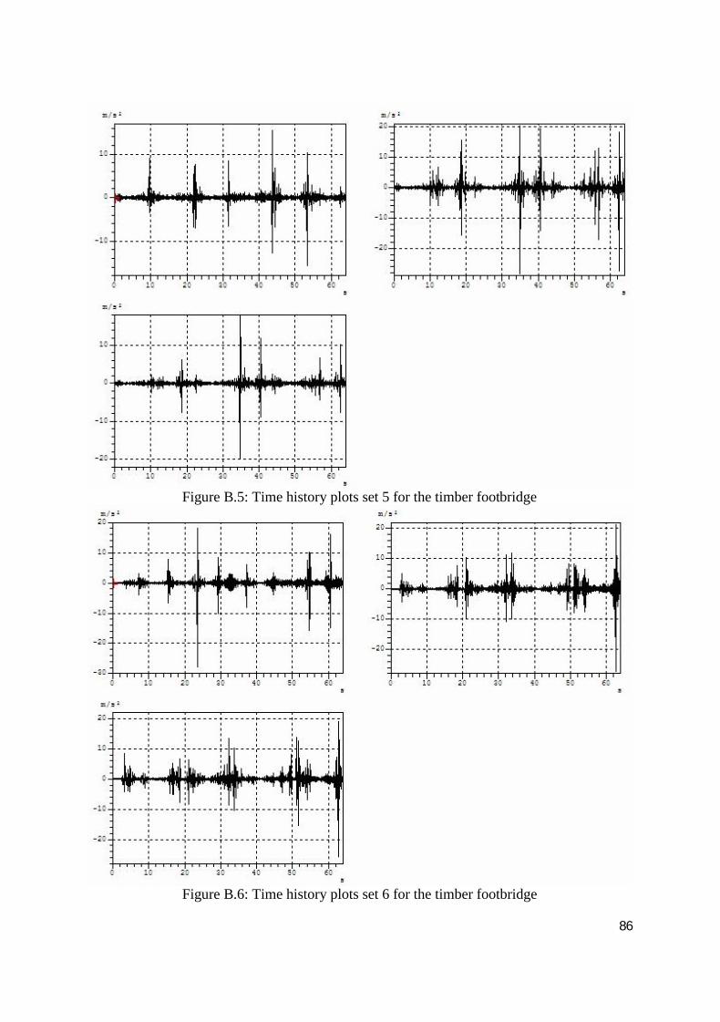
86

Figure B.5: Time history plots set 5 for the timber footbridge

Figure B.6: Time history plots set 6 for the timber footbridge

87

Figure B.7: Time history plots set 7 for the timber footbridge

Figure B.8: Time history plots set 8 for the timber footbridge

88

Time History Plots for Concrete Bridge

Figure B.9: Time history plots set 1 for the concrete footbridge

Figure B.10: Time history plots set 2 for the concrete footbridge

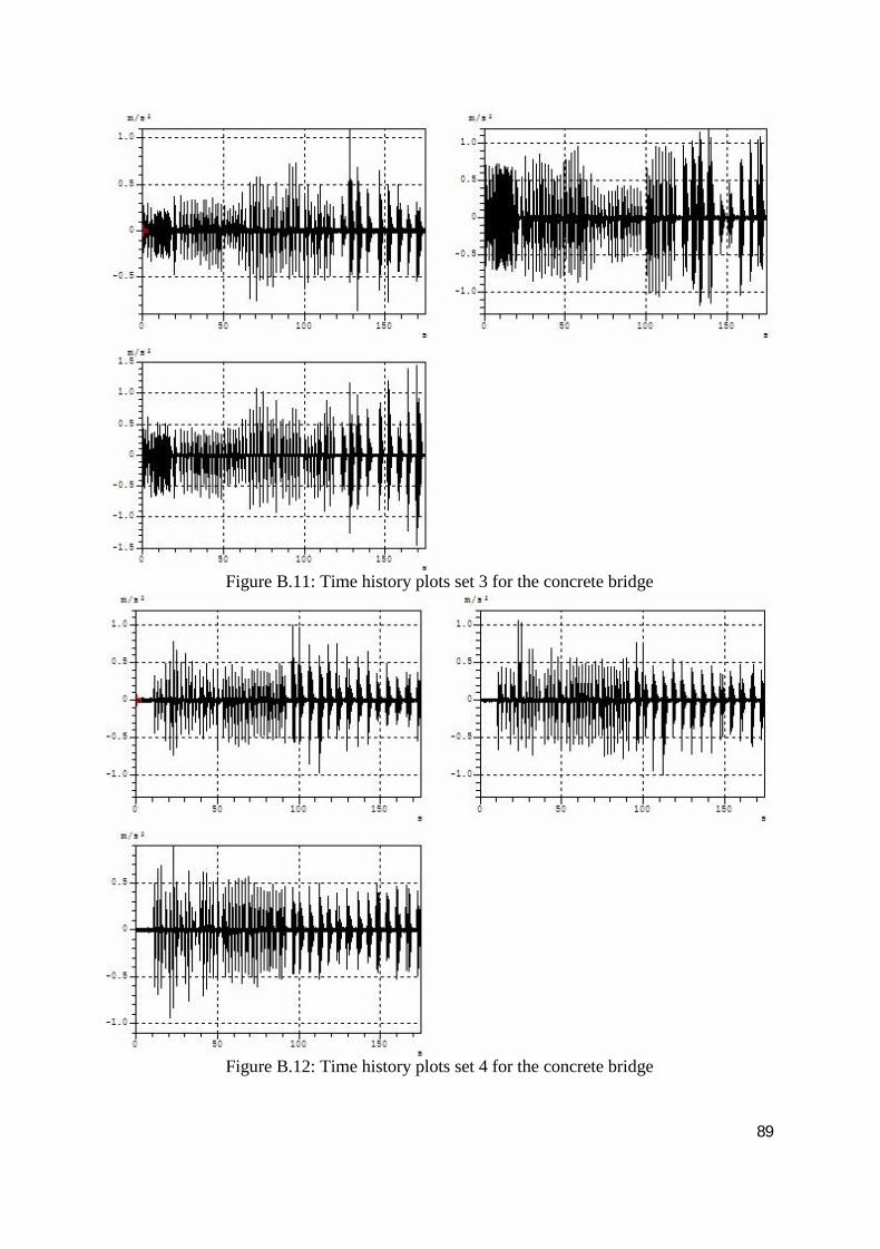
89

Figure B.11: Time history plots set 3 for the concrete bridge

Figure B.12: Time history plots set 4 for the concrete bridge

90

Figure B.13: Time history plots set 5 for the concrete bridge

Figure B.14: Time history plots set 6 for the concrete bridge

91

Figure B.15: Time history plots set 7 for the concrete bridge

Figure B.16: Time history plots set 8 for the concrete bridge

92

Figure B.17: Time history plots set 9 for the concrete bridge

Figure B.18: Time history plots set 10 for the concrete bridge

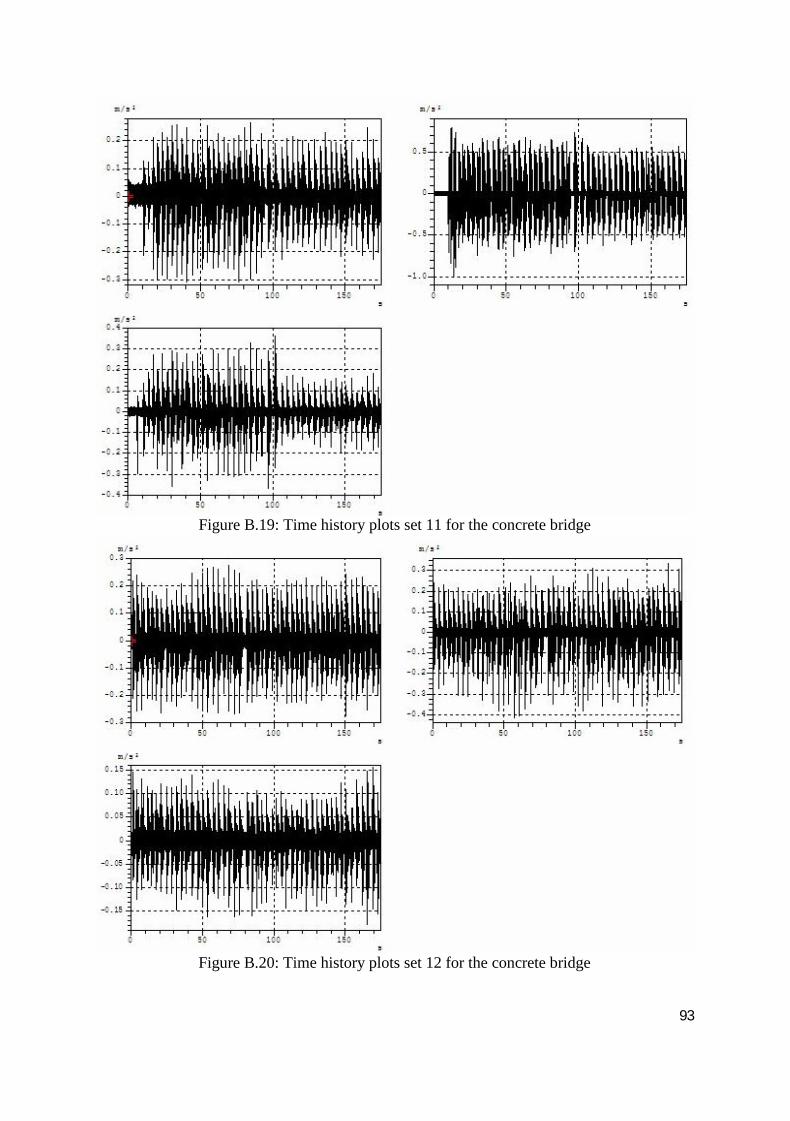
93

Figure B.19: Time history plots set 11 for the concrete bridge

Figure B.20: Time history plots set 12 for the concrete bridge

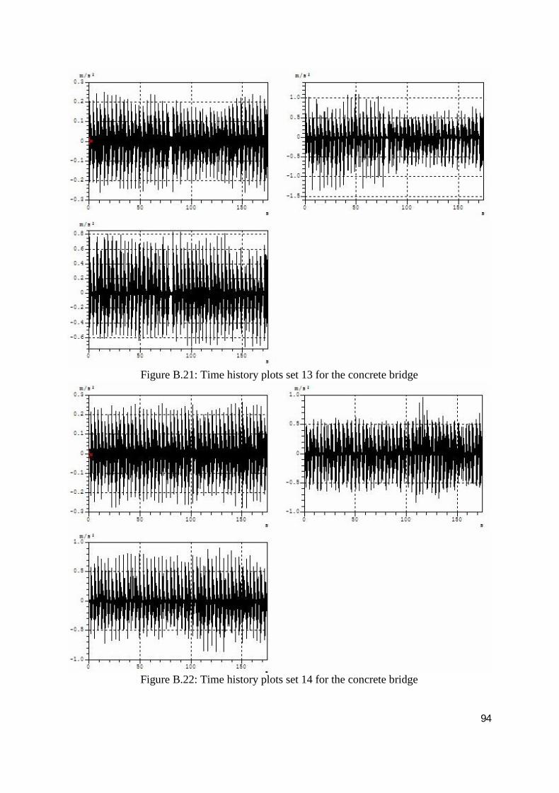
94

Figure B.21: Time history plots set 13 for the concrete bridge

Figure B.22: Time history plots set 14 for the concrete bridge

95

Figure B.23: Time history plots set 15 for the concrete bridge

Figure B.24 Time history plots set 16 for the concrete bridge

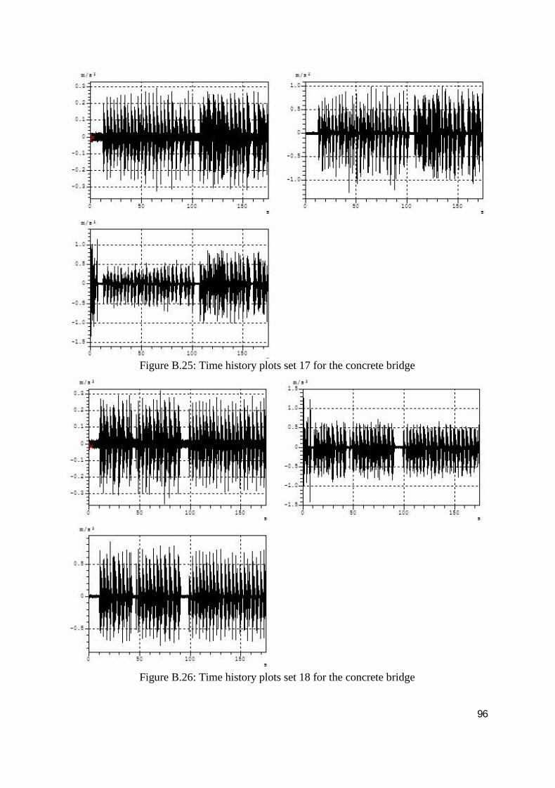
96

Figure B.25: Time history plots set 17 for the concrete bridge

Figure B.26: Time history plots set 18 for the concrete bridge

97

Figure B.27: Time history plots set 19 for the concrete bridge

Figure B.28: Time history plots set 20 for the concrete bridge

98

Appendix C

ANSYS commands for the Staircase Structure

/FILNAM,FKM Staircase/title, FKM Staircase/prep7/VUP,1,Z/VIEW,1,1,-1,1/replot!Create geometry of staircase!Keypoints of staircasek, 100, 0.0000000000, 0.0000000000, 0.0000000000k, 101,-0.0328271710, 0.0000000000, 0.2175000000k, 102, 0.2121728290, 0.0000000000, 0.2175000000k, 103, 0.1921728290, 0.0000000000, 0.3625000000k, 104, 0.4571728290, 0.0000000000, 0.3625000000k, 105, 0.4371728290, 0.0000000000, 0.5125000000k, 106, 0.7096728290, 0.0000000000, 0.5125000000k, 107, 0.6896728290, 0.0000000000, 0.6625000000k, 108, 0.9546728290, 0.0000000000, 0.6625000000k, 109, 0.9346728290, 0.0000000000, 0.8150000000k, 110, 1.1996728290, 0.0000000000, 0.8150000000k, 111, 1.1796728290, 0.0000000000, 0.9675000000k, 112, 1.4346728290, 0.0000000000, 0.9675000000k, 113, 1.4146728290, 0.0000000000, 1.1150000000k, 114, 1.6846728290, 0.0000000000, 1.1150000000k, 115, 1.6646728290, 0.0000000000, 1.2650000000k, 116, 1.9246728290, 0.0000000000, 1.2650000000k, 117, 1.9046728290, 0.0000000000, 1.4200000000k, 118, 2.1746728290, 0.0000000000, 1.4200000000k, 119, 2.1521728290, 0.0000000000, 1.5700000000k, 120, 2.4071728290, 0.0000000000, 1.5700000000k, 121, 2.3871728290, 0.0000000000, 1.7200000000k, 122, 2.6521728290, 0.0000000000, 1.7200000000k, 123, 2.6321728290, 0.0000000000, 1.8725000000k, 124, 2.8796728290, 0.0000000000, 1.8725000000k, 125, 2.8602152019, 0.0000000000, 2.0125000000k, 126, 3.1016728290, 0.0000000000, 2.0125000000k, 127, 3.1016728290, 0.0000000000, 2.1725000000k, 128, 4.6716728290, 0.0000000000, 2.1725000000k, 129, 4.6716728290, 0.0000000000, 2.0125000000k, 130, 3.9916728290, 0.0000000000, 2.0125000000k, 131, 3.9916728290, 0.0000000000, 1.8675000000k, 132, 3.7416728290, 0.0000000000, 1.8675000000k, 133, 3.7416728290, 0.0000000000, 2.0125000000k, 134, 3.3916728290, 0.0000000000, 2.0125000000k, 135, 0.2082644921, 0.0000000000, 0.0000000000

99

k, 200, 3.1016728290, 1.4950000000, 2.0125000000k, 201, 3.1016728290, 1.4950000000, 2.1725000000k, 202, 2.8816728290, 1.4950000000, 2.1725000000k, 203, 2.9016728290, 1.4950000000, 2.3300000000k, 204, 2.6416728290, 1.4950000000, 2.3300000000k, 205, 2.6616728290, 1.4950000000, 2.4800000000k, 206, 2.3991728290, 1.4950000000, 2.4800000000k, 207, 2.4191728290, 1.4950000000, 2.6400000000k, 208, 2.1716728290, 1.4950000000, 2.6400000000k, 209, 2.1916728290, 1.4950000000, 2.7825000000k, 210, 1.9241728290, 1.4950000000, 2.7825000000k, 211, 1.9441728290, 1.4950000000, 2.9375000000k, 212, 1.6966728290, 1.4950000000, 2.9375000000k, 213, 1.7166728290, 1.4950000000, 3.1000000000k, 214, 1.4641728290, 1.4950000000, 3.1000000000k, 215, 1.4841728290, 1.4950000000, 3.2525000000k, 216, 1.2216728290, 1.4950000000, 3.2525000000k, 217, 1.2416728290, 1.4950000000, 3.4025000000k, 218, 0.9916728290, 1.4950000000, 3.4025000000k, 219, 1.0116728290, 1.4950000000, 3.5550000000k, 220, 0.7466728290, 1.4950000000, 3.5550000000k, 221, 0.7666728290, 1.4950000000, 3.7025000000k, 222, 0.5166728290, 1.4950000000, 3.7025000000k, 223, 0.5366728290, 1.4950000000, 3.8550000000k, 224, 0.2691728290, 1.4950000000, 3.8550000000k, 225, 0.2891728290, 1.4950000000, 4.0200000000k, 226, 0.0316728290, 1.4950000000, 4.0200000000k, 227, 0.0516728290, 1.4950000000, 4.1775000000k, 228,-0.2183271710, 1.4950000000, 4.1775000000k, 229,-0.1983271710, 1.4950000000, 4.3525000000k, 230,-0.8482031551, 1.4950000000, 4.3525000000k, 231,-0.8482031551, 1.4950000000, 4.1925000000k, 232,-0.5913737601, 1.4950000000, 4.1925000000k, 233, 2.7791998060, 1.4950000000, 2.0125000000k, 234,-0.2183271710, 1.4950000000, 3.9512230932k, 300,3.7416728290, 1.26, 0.0k, 301,3.9916728290, 1.26, 0.0k, 302,3.9916728290, 1.51, 0.0k, 303,3.7416728290, 1.51, 0.0! Area for Stair Landing and beam (Area no 1)A,126,127,128,129,130,131,132,133,134! Area for column base (Area no 2)A,300,301,302,303! Area for Upper Stairs (Area no 3 & 4)A,200,201,202,203,204,205,206,207,208,209,210,211,212,213,214,215,216,233A,216,217,218,219,220,221,222,223,224,225,226,227,228,234,233

100

! Area for Lower Stairs (Area no 5 & 6)A,100,101,102,103,104,105,106,107,108,109,110,111,112,113,114,115,116,135A,116,117,118,119,120,121,122,123,124,125,126,134,135

! Combine Area 5 & 6 = 7AADD,5,6

! Combine Area 3 & 4 = 5AADD,3,4APLOT

! Create Stairs of length 1.275m in the y-dir by extrude area (Area No 1,2,3 & 4) intoVolume

! VEXT, NA1, NA2, NINC, DX, DY, DZ, RX, RY, RZVEXT, 5, 7, 2, 0, 1.275, 0, 0, 0, 0

! Create Landing of length 2.77m in the Y-dirVEXT,1, , ,0,2.77,0,,,,

! Create Column of length 1.8675m in the z-dirVEXT,2, , ,0,0,1.8675,,,,

! Combine all the volumes of straicase!VGLUE,ALL

! Material Properties of staircaseET,1,SOLID92

!*!*MPTEMP,,,,,,,,MPTEMP,1,0MPDATA,EX,1,,24.5e9MPDATA,PRXY,1,,.2MPTEMP,,,,,,,,MPTEMP,1,0MPDATA,DENS,1,,2400! Boundary condition for staircaseDA,2,ALLDA,18,ALLDA,50,ALL!EMATWRITE,YESVSEL,S,,,1,4,1VADD,ALL

101

! Meshing of staircaseSMRTSIZE,5MSHKEY,0VMESH,ALL

/SOLU!Modal solution (20 modes)ANTYPE,2MODOPT,SUBSP,20OUTRES,ALL,ALL,MXPAND,20SOLVE

ANSYS commands for the Timber bridge/FILNAM,UTMTimberBridge/title, UTM Timber Bridge/prep7/VUP,1,Z/VIEW,1,1,-1,1/replot

!Define Element Types and PropertiesET,1,BEAM4ET,2,shell63

!Define real constants

!Steel GirderR,1,4.775e-5,8.747e-5,7.4899e-6,.315,.165, ,RMORE, ,1.0825e-7, , , , ,

!RHS 150x85x10R,2,4.3e-3,4.7015e-6,1.2006e-5,85,150, ,RMORE, ,1.02723e-5, , , , ,

!RHS 150x75x10R,3,4.1e-3,1.1024e-5,3.471e-6, , , ,RMORE, ,8.4769e-6, , , , ,

!Timber Plank assumed as SlabR,4,0.04

102

!Steel SectionMPTEMP,,,,,,,,MPTEMP,1,0MPDATA,EX,1,,200e9MPDATA,PRXY,1,,.3MPTEMP,,,,,,,,MPTEMP,1,0MPDATA,DENS,1,,7850

!TimberMPTEMP,,,,,,,,MPTEMP,1,0MPDATA,EX,2,,19e9MPDATA,PRXY,2,,0.2MPTEMP,,,,,,,,MPTEMP,1,0MPDATA,DENS,2,,980

!Create geometry!Keypoints

K,1,0,0,0,K,2,0,0.4975,0, !SupportK,3,0,3.5775,0,K,4,0,7.1375,0,K,5,0,10.6625,0,K,6,0,13.7425,0, !SupportK,7,0,14.2400,0,

K,8,0.8425,0,0,K,9,0.8425,0.4975,0,K,10,0.8425,3.5775,0,K,11,0.8425,7.1375,0,K,12,0.8425,10.6625,0,K,13,0.8425,13.7425,0,K,14,0.8425,14.2400,0,

K,15,1.685,0,0,K,16,1.685,0.4975,0, !SupportK,17,1.685,3.5775,0,K,18,1.685,7.1375,0,K,19,1.685,10.6625,0,K,20,1.685,13.7425,0, !SupportK,21,1.685,14.2400,0,

!k,22,0,0.1025,0!k,23,1.85,0.1025,0

103

!Line Definition

numstr,line,101l,1,2l,2,3l,3,4l,4,5l,5,6l,6,7l,15,16l,16,17l,17,18l,18,19l,19,20l,20,21

numstr,line,201l,8,9l,9,10l,10,11l,11,12l,12,13l,13,14

!numstr,line,301!l,1,8!l,8,15!l,7,14!l,14,21

numstr,line,401l,1,8l,8,15l,2,9l,9,16l,3,10l,10,17l,4,11l,11,18l,5,12l,12,19l,6,13l,13,20l,7,14l,14,21

104

!Assign Real Constants and Material Properties

lsel,s,,,101,112,1latt,1,1,1

lsel,s,,,201,206,1latt,1,2,1

lsel,s,,,403,412,1latt,1,3,1

!lsel,s,,,301!latt,2,4,1

Allsel

!Generate shells

numstr,area,2001al,101,403,201,401 ! count+100,count+402,count+200,count+400al,102,405,202,403al,103,407,203,405al,104,409,204,407al,105,411,205,409al,106,413,206,411

al,201,404,107,402al,202,406,108,404al,203,408,109,406al,204,410,110,408al,205,412,111,410al,206,414,112,412asel,s,,,2001,2012aatt,2,4,2

allsellsel,s,,,401,414lesize,all,,,3lsel,s,,,102,105lsel,a,,,108,111lesize,all,,,10lsel,s,,,202,205lesize,all,,,10

105

lsel,s,,,101lsel,a,,,201lsel,a,,,107lsel,s,,,106lsel,a,,,206lsel,a,,,112lesize,all,,,2

lmesh,allamesh,all

!Boundary Conditionksel,s,,,2ksel,a,,,6ksel,a,,,16ksel,a,,,20dk,all,all,0

/SOLU!Modal solution (20 modes)ANTYPE,2MODOPT,SUBSP,20OUTRES,ALL,ALL,MXPAND,20

allselsolve

ANSYS commands for the Concrete Bridge

/FILNAM,Bridge/title, GerbangBridge/prep7/VUP,1,Z/VIEW,1,1,-1,1/replot

!Bridge GeometryLd = 10.8Bd = 0.5Xd = 0.75Hd = 0.5Lb = 10.8Bb = 0.5Hb = 0.528Sd = 0.013BTB= 0.513

106

! Create geometry

! Keypoints

K,1,0,0,0,K,2,Bb,0,0,K,3,0,0,Hb,K,4,Bb,0,Hb,K,5,-Xd,0,Hb,K,6,-Xd,0,Hb+Hd,K,7,0,0,Hb+Hd,K,8,Bd,0,Hb+Hd,K,9,Bd+Sd,0,Hb,K,10,Bd+Sd,0,Hb+Hd,

! Create AreasA,1,2,4,3 !Area no 1A,5,3,7,6 !Area no 2A,3,4,8,7 !Area no 3A,4,9,10,8 !Area no 4

! Create VolumeVEXT,1,,1,0,Lb,0VEXT,2,4,1,0,Ld,0

! Generate VolumeVGEN,39,1, , ,BTB, , , ,1VGEN,39,3, , ,BTB, , , ,1VGEN,38,4, , ,BTB, , , ,1VGEN,2,2, , ,20.744, , , ,1

! Structural elementET,1,SOLID185MPTEMP,,,,,,,,MPTEMP,1,0MPDATA,EX,1,,24.5e9MPDATA,PRXY,1,,.2MPTEMP,,,,,,,,MPTEMP,1,0MPDATA,DENS,1,,2400MPTEMP,,,,,,,,MPTEMP,1,0MPDATA,EX,2,,30.1e9MPDATA,PRXY,2,,.2MPTEMP,,,,,,,,MPTEMP,1,0MPDATA,DENS,2,,2400

107

VGLUE,ALL

! select element atrributeVSEL,s,,,119,122VATT,1,,1

VSEL,s,,,124,198VATT,1,,1

VSEL,s,,,1VATT,2,,1

VSEL,s,,,123VATT,2,,1

VSEL,s,,,6,42VATT,2,,1

Allsel! Boundary conditionASEL,s,,,1,5,1DA,ALL,ALL

ASEL,s,,,29,245,6DA,ALL,ALL

ASEL,s,,,722,866,4DA,ALL,ALL

ASEL,s,,,876,1020,4DA,ALL,ALL

ASEL,s,,,714,720,6DA,ALL,ALL

ASEL,s,,,872,873,1DA,ALL,ALL

ASEL,s,,,30,246,6DA,ALL,ALL

ASEL,s,,,723,867,4DA,ALL,ALL

ASEL,s,,,709,715,6DA,ALL,ALL

ASEL,s,,,711,713,2DA,ALL,ALL

108

ASEL,s,,,713,,1DA,ALL,ALL

ASEL,s,,,721,,1DA,ALL,ALL

ASEL,s,,,877,1021,4DA,ALL,ALL

allsel! Define element divisions

! sideLESIZE,5,,,3LESIZE,1568,,,3LESIZE,3,,,2LESIZE,1412,,,2

! widthLESIZE,4,,,2LESIZE,6,,,2LESIZE,12,,,2LESIZE,1418,,,2LESIZE,1397,,,2LESIZE,485,,,2

! small widthLESIZE,13,,,1LESIZE,29,,,8LESIZE,26,,,8LSEL,s,,,55,487,12LESIZE,ALL,,,2LSEL,s,,,1421,1565,4LESIZE,ALL,,,2LSEL,s,,,54,486,12LESIZE,ALL,,,2LSEL,s,,,1574,1718,4LESIZE,ALL,,,1

Allsel

! Meshing for bridgeMSHAPE,0,3d !Mapped meshMSHKEY,1VMESH,allMSHKEY,0

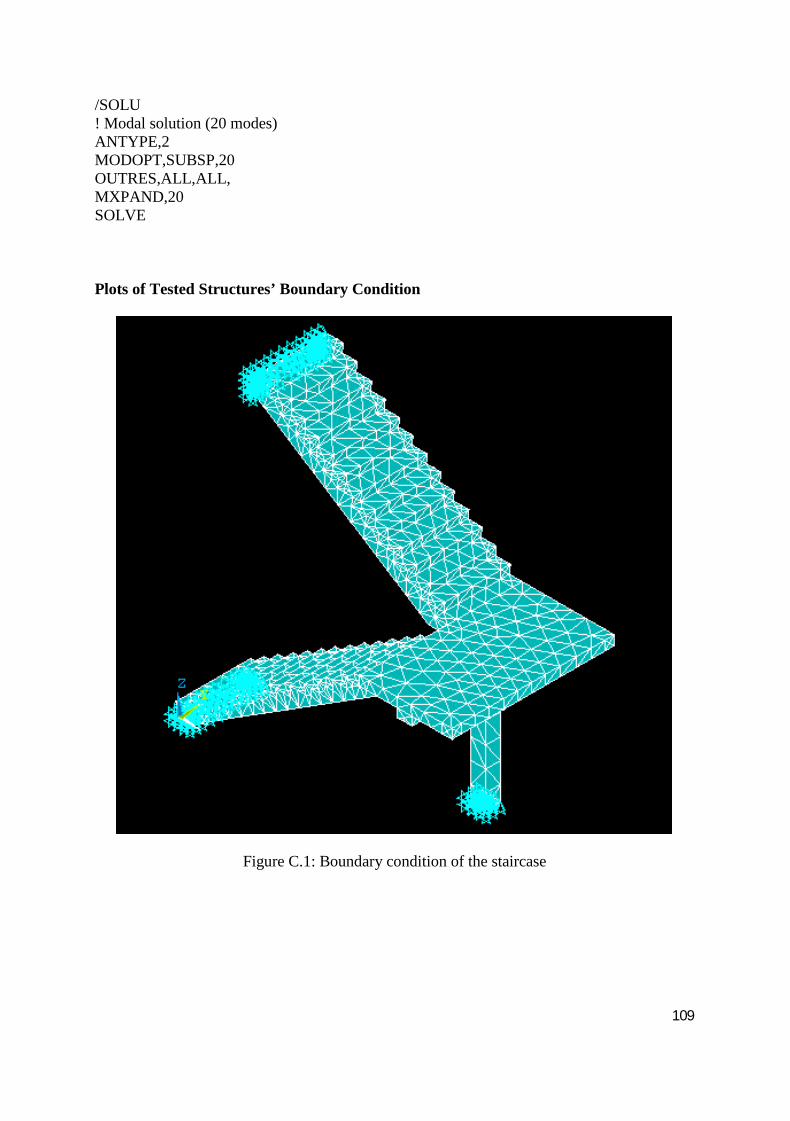
109

/SOLU! Modal solution (20 modes)ANTYPE,2MODOPT,SUBSP,20OUTRES,ALL,ALL,MXPAND,20SOLVE

Plots of Tested Structures’ Boundary Condition

Figure C.1: Boundary condition of the staircase

110

Figure C.2: Boundary condition of the timber footbridge

Figure C.3: Boundary condition of the concrete bridge

111

Appendix D

Peak Picking SV Plot for the Staircase Structure

112

Peak Picking SV Plot for the Timber Footbridge

113

Peak Picking SV Plot for the Concrete Bridge