MIXED-LOAD AT VOLVO POWERTRAIN An Investigation of Small Packages and Transportation Routes to Provide a Leaner Material Flow for Volvo Powertrain’s Assembly Factory in Skövde Master of Science Thesis Authors: M. ALPER ÇORAKÇI AYŞE DİNÇER Examiner: LARS MEDBO Supervisor: CHRISTIAN FINNSGÅRD Department of Technology Management and Economics Division of Transportation and Logistics CHALMERS UNIVERSITY OF TECHNOLOGY Göteborg, Sweden, 2008 Report No E2008:049

Welcome message from author
This document is posted to help you gain knowledge. Please leave a comment to let me know what you think about it! Share it to your friends and learn new things together.
Transcript
MIXED-LOAD AT VOLVO POWERTRAIN
An Investigation of Small Packages and Transportation Routes to Provide a Leaner Material Flow for Volvo Powertrain’s Assembly Factory in Skövde
Master of Science Thesis
Authors: M. ALPER ÇORAKÇI AYŞE DİNÇER
Examiner: LARS MEDBO
Supervisor: CHRISTIAN FINNSGÅRD
Department of Technology Management and Economics Division of Transportation and LogisticsCHALMERS UNIVERSITY OF TECHNOLOGYGöteborg, Sweden, 2008
Report No E2008:049
Chalmers University of Technology
Dedication
This thesis work is dedicated to my mother E. Gülay, father M.Hilmi, and sister A.Özge whose sacrifices, which were realized by our loss of precious time together, were the most painful and yearning for me.
I have felt their true love, trust and support with me throughout my entire life. Without them i could not be the person i am.
M. Alper Çorakçı
To my parents, my brother Ahmet, my friends Murat and Rafiye for all their support, positive energy and love.
Ayşe Dinçer
Chalmers University of Technology
ACKNOWLEDGEMENTS
This Master Thesis is carried out at Volvo Powertrain in Skövde for the master’s degree at Chalmers University of Technology. The work has been performed between October 2007 and March 2008.
We have special thanks for our supervisor Christian Finnsgård from Chalmers University of Technology for supporting us all the time during the thesis with his knowledge and experience in the logistics area. He kept us always motivated and changed our moods positively in the difficult times.
We also have special thanks to our supervisor Anders Wiik from Volvo Powertrain for guiding us in the company all the time during the thesis. He motivated us to think out of the box and let us to focus on the areas that we really want to work on. He also supported us to find the right contact in and outside of the factory.
Besides, we would like to thank all the people who helped us via personal contacts and interviews especially to Stellan Galle, Per Weinö and Anders Nilsson.
We feel that this thesis has been very exciting and informative for us and helped us to broaden our knowledge and experience in the area. We hope this thesis is going to help Volvo Powertrain to shape their decisions related to material flow of their assembly factory.
Göteborg, March 2008
Chalmers University of Technology
ABSTRACT
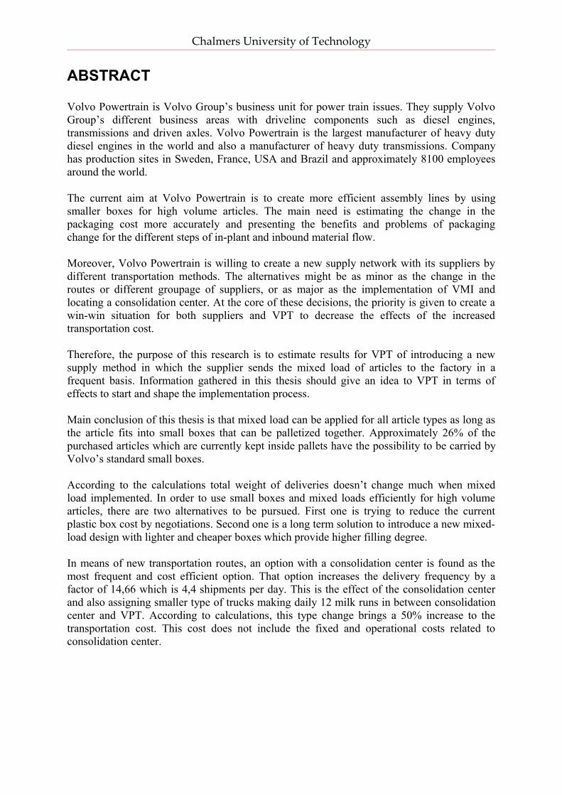
Volvo Powertrain is Volvo Group’s business unit for power train issues. They supply Volvo Group’s different business areas with driveline components such as diesel engines, transmissions and driven axles. Volvo Powertrain is the largest manufacturer of heavy duty diesel engines in the world and also a manufacturer of heavy duty transmissions. Company has production sites in Sweden, France, USA and Brazil and approximately 8100 employees around the world.
The current aim at Volvo Powertrain is to create more efficient assembly lines by using smaller boxes for high volume articles. The main need is estimating the change in the packaging cost more accurately and presenting the benefits and problems of packaging change for the different steps of in-plant and inbound material flow.
Moreover, Volvo Powertrain is willing to create a new supply network with its suppliers by different transportation methods. The alternatives might be as minor as the change in the routes or different groupage of suppliers, or as major as the implementation of VMI and locating a consolidation center. At the core of these decisions, the priority is given to create a win-win situation for both suppliers and VPT to decrease the effects of the increased transportation cost. Therefore, the purpose of this research is to estimate results for VPT of introducing a new supply method in which the supplier sends the mixed load of articles to the factory in a frequent basis. Information gathered in this thesis should give an idea to VPT in terms of effects to start and shape the implementation process.
Main conclusion of this thesis is that mixed load can be applied for all article types as long as the article fits into small boxes that can be palletized together. Approximately 26% of the purchased articles which are currently kept inside pallets have the possibility to be carried by Volvo’s standard small boxes.
According to the calculations total weight of deliveries doesn’t change much when mixed load implemented. In order to use small boxes and mixed loads efficiently for high volume articles, there are two alternatives to be pursued. First one is trying to reduce the current plastic box cost by negotiations. Second one is a long term solution to introduce a new mixed-load design with lighter and cheaper boxes which provide higher filling degree.
In means of new transportation routes, an option with a consolidation center is found as the most frequent and cost efficient option. That option increases the delivery frequency by a factor of 14,66 which is 4,4 shipments per day. This is the effect of the consolidation center and also assigning smaller type of trucks making daily 12 milk runs in between consolidation center and VPT. According to calculations, this type change brings a 50% increase to the transportation cost. This cost does not include the fixed and operational costs related to consolidation center.
Chalmers University of Technology
TABLE OF CONTENTS
1. INTRODUCTION ................................................................... 10 1.1 The Company Overview ......................................................................................... 10 1.2 Problem Background ............................................................................................... 11 1.3 Purpose .................................................................................................................... 12 1.4 Research Questions ................................................................................................. 12 1.5 Limitations .............................................................................................................. 12
2. METHODOLOGY .................................................................. 13 2.1 Research Method ..................................................................................................... 13 2.2 Research Design ...................................................................................................... 13 2.3 Data Collection ........................................................................................................ 14 2.4 The Value of the Results ......................................................................................... 15
3. THEORETICAL FRAMEWORK .......................................... 16 3.1 Lean Thinking ......................................................................................................... 16
3.1.1 Principles of Lean Thinking ..................................................................................... 16 3.1.2 Waste Elimination in Lean Thinking ....................................................................... 17
3.2 Lean Logistics ......................................................................................................... 18 3.2.1 Logistics .................................................................................................................. 18 3.2.2 World Class Logistics .............................................................................................. 19 3.2.1 Inbound and outbound logistics ............................................................................... 20 3.2.2 In - plant Logistics and Material Handling .............................................................. 21
3.3 Material Flow Control ............................................................................................. 21 3.3.1 Cycle Time and Takt Time ...................................................................................... 22 3.3.2 Creating the one-piece flow ..................................................................................... 22
3.4 Packaging Logistics ................................................................................................ 24 3.4.1 Demands on Packaging ............................................................................................ 24
3.4.2 Mixed Load ........................................................................................................ 26 3.5 Transportation ......................................................................................................... 27
3.5.1 Direct Shipment ....................................................................................................... 27 3.5.2 Consolidation Center ................................................................................................ 28
3.5.2.1 ABC Classification ......................................................................................... 29 3.5.2.2 Facility Location ............................................................................................. 29
3.5.3 Mixed Transportation .............................................................................................. 30 3.6 Transportation Cost ................................................................................................. 33
3.6.1 Transportation Cost Structure .................................................................................. 33 3.6.2 Transportation Cost Parameters ............................................................................... 33 3.6.3 Road Transportation ................................................................................................. 35
3.7 Supplier Relations ................................................................................................... 36 3.7.1 Vendor Managed Inventory (VMI) ......................................................................... 36 3.7.2 Vendor Managed Replenishment (VMR) ................................................................ 37
4. PRESENT SITUATION ......................................................... 38 4.1 Packaging and Mixed Load ..................................................................................... 38
4.1.1 Packaging ................................................................................................................ 38 4.1.2 Mixed Loads ............................................................................................................ 39
4.2 In-plant logistics ...................................................................................................... 40 4.2.1 Production ................................................................................................................ 40 4.2.2 Supermarket ............................................................................................................. 41
Chalmers University of Technology
4.2.3 Internal Material Flow and Material Feeding ......................................................... 43 4.2.4 Warehousing ............................................................................................................ 43 4.2.5 ID station .................................................................................................................. 44 4.2.6 Goods receiving ....................................................................................................... 44
4.3 Material Controlling ................................................................................................ 44 4.3.1 Internal Material Control ....................................................................................... 45 4.3.2 External Material Control ....................................................................................... 45
4.4 Transportation ......................................................................................................... 46 4.4.1 Mixed Transportation ............................................................................................... 48 4.4.2 Transportation Agreements and Ownership ............................................................ 49
5. ALTERNATIVE SYSTEM DESIGN ...................................... 50 5.1 Smaller Package ..................................................................................................... 50
5.1.1 Data Collection Process ........................................................................................... 51 5.1.2 Result of the Data Collection ................................................................................... 51
5.2 Mixed Load ............................................................................................................. 52 5.2.1 Mixed Load Estimations and Calculations for Current System ............................... 52
5.2.1.1 Mixed-load Pallet Type and Number of Inner Packages Estimation ............. 52 5.2.1.2 Volume estimations ........................................................................................ 53 5.2.1.3 Weight estimation ........................................................................................... 54 5.2.1.4 Packaging transaction fee cost ....................................................................... 54
5.2.2 Mixed Load Estimations and Calculations for the Alternative System ................... 55 5.3 Inbound Logistics ................................................................................................... 56
5.3.1 Sub-System Formation ............................................................................................. 56 5.3.1.1 Current Cost Calculation Methodology ......................................................... 57
5.3.2 Assumptions for Transportation Mode ................................................................... 57 5.3.3 Assumptions for Transportation Costs ..................................................................... 59 5.3.4 Sub-system Scenarios ............................................................................................. 61
5.3.4.1 Scenario 1 ........................................................................................................ 61 5.3.4.2.1 The Location of Consolidation Center ................................................... 63 5.3.4.2.2 Milk Runs between VPT and Consolidation Center ............................... 64
5.3.4.3 Scenario 3 ........................................................................................................ 65 5.3.4.3.1 Milk Run 1 .............................................................................................. 65 5.3.4.3.2 Milk Run 2 ............................................................................................. 66 5.3.4.3.3 Milk Run 3 ............................................................................................. 67
6. RESULTS & ANALYSIS ..................................................... 68 6.1 Small Package and Mixed Load .............................................................................. 69
6.1.1 Eligibility of Smaller Packages ................................................................................ 69 6.1.2 Mixed Load ............................................................................................................. 70 6.1.3 Problems with available packages ........................................................................... 71
6.1.3.1 Problems with cartoon boxes .......................................................................... 72 6.1.3.2 Problems with pallets ...................................................................................... 72 6.1.3.3 Problems with blue boxes ............................................................................... 72 6.1.3.4 Problems with mixed-load design ................................................................... 74
6.1.5 Effects of smaller packages ...................................................................................... 74 6.1.5.1 Effects on production ............................................................................................ 74
6.1.5.2 Effects on internal transportation .................................................................... 75 6.1.5.3 Effects on warehousing .................................................................................. 75
6.2 Inbound Logistics Flow Analysis ............................................................................ 75 6.2.1 Total Cost Calculation for Scenario 1 ...................................................................... 76 6.2.2 Total Cost Calculation for Scenario 2 ...................................................................... 77
Chalmers University of Technology
6.2.2.1 Problems related to Consolidation Center ...................................................... 78 6.2.3 Total Cost of Scenario 3 ........................................................................................... 78
6.2.3.1 Problems with Milk Runs ............................................................................... 79 6.2.4 Comparison of Scenarios with Current Situation .................................................... 79
7. CONCLUSION ...................................................................... 81 8. RECOMMENDATIONS ........................................................ 83
8.1 Design of a more efficient mixed-load with new boxes ......................................... 83 8.2 Recommendations on Consolidation Center ........................................................... 83 8.3 Recommendations on Milk Runs ............................................................................ 84 8.4 Recommendations for Future Research .................................................................. 84
REFERENCE LIST ................................................................... 85
Chalmers University of Technology
List of Abbreviations 3PL – Third Party Logistics Provider
Dn – Total distance traveled by vehicle n (km)
EMS – Emergent Market Sourcing
Fn – Hourly fuel consumption for vehicle n (gr/km)
FC – Total Fuel Consumption Cost
FCA – Free Carrier
GAMA – Golden State Automotive Manufacturers Association
GPT – Global Packaging Tool
H – Number of handling
Hc – Average handling Cost
HC – Total Handling Cost
LTL – Less Than Truck Load
NUMMI – New United Motor Manufacturing Incorporation
Rn – Daily rent of vehicle n including driver’s wage
Rn’ – Daily rent of vehicle n excluding driver’s wage
TC – Total Cost of Transportation
TL – Truck Load
Tn – Total Time vehicle n is on transport (mins)
VC – Total Vehicle Renting Cost
VLC – Volvo Logistics
VMI – Vendor Managed Inventory
VMR – Vendor Managed Replenishment
VPT – Volvo Powertrain in Skövde
Chalmers University of Technology
1. INTRODUCTION
The first chapter introduces the reader to the thesis content. First, a detailed company overview about Volvo Powertrain is provided. Thereafter, background of the problem is presented. Furthermore, the purpose, scope and limitations of this thesis are clarified in order to be able to formulate the problem correctly.
1.1 The Company Overview
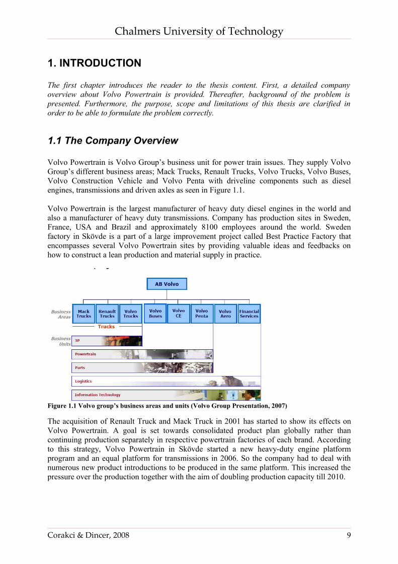
Volvo Powertrain is Volvo Group’s business unit for power train issues. They supply Volvo Group’s different business areas; Mack Trucks, Renault Trucks, Volvo Trucks, Volvo Buses, Volvo Construction Vehicle and Volvo Penta with driveline components such as diesel engines, transmissions and driven axles as seen in Figure 1.1.
Volvo Powertrain is the largest manufacturer of heavy duty diesel engines in the world and also a manufacturer of heavy duty transmissions. Company has production sites in Sweden, France, USA and Brazil and approximately 8100 employees around the world. Sweden factory in Skövde is a part of a large improvement project called Best Practice Factory that encompasses several Volvo Powertrain sites by providing valuable ideas and feedbacks on how to construct a lean production and material supply in practice.
Figure 1.1 Volvo group’s business areas and units (Volvo Group Presentation, 2007)
The acquisition of Renault Truck and Mack Truck in 2001 has started to show its effects on Volvo Powertrain. A goal is set towards consolidated product plan globally rather than continuing production separately in respective powertrain factories of each brand. According to this strategy, Volvo Powertrain in Skövde started a new heavy-duty engine platform program and an equal platform for transmissions in 2006. So the company had to deal with numerous new product introductions to be produced in the same platform. This increased the pressure over the production together with the aim of doubling production capacity till 2010.
Corakci & Dincer, 2008 9
Chalmers University of Technology
1.2 Problem Background
The increasing internationalization in the business environment and rapid changes in the customer demands have started to force companies to improve in many areas. For example there has been a push towards lower inventories, faster response, mass customization and lower transaction costs in the automotive industry due to high competitive market combined with short life cycles of articles and products. VPT, as a prospering company, has acknowledged the trend and aims to react upon by putting into operation a more customer focused and leaner concept. For this purpose, Lean Material Handling Project on the agenda focuses on constructing a leaner material supply system by pushing inventories back towards the suppliers, as a way of reducing the total waste in the system.
First step of this process was the Lean Assembly Line project which aims to reengineer assembly stations in a way to decrease non-value adding time by achieving an ergonomic and efficient picking. This has planned to be done by replacing pallets with smaller boxes to expose the materials in the assembly stations since pallets are space-consuming and using them will result in having longer and higher material racks where picking is not efficient. When the stations are more efficient and well balanced then there is less waste in terms of tied-up capital, movement of assemblers and waiting times. This will create a smooth flow where productivity levels are increased and response times are improved.
Second step is to be able to feed stations with smaller boxes. This is planned to be solved in two ways:
First solution is repacking pallets into boxes in a temporary storage called supermarket and sending boxes to the stations whenever they are needed. VPT has implemented this solution for 390-400 articles already. However, repacking can be considered as a waste since packaging changes two times in the system until they get to the point of use.
Second solution aims to eliminate the repacking efforts by receiving articles in small boxes directly from suppliers. These boxes are put together onto pallets whether or not there are same articles inside each of them. This concept is called mixed load and has being used in the industry for years. The company has realized that smaller packages and mixed load concept can reduce the waste of excess space at the assembly stations for the low volume articles. So, they already started to implement packaging changes.
The current aim is to carry the project one step further and to create even more efficient assembly lines by using smaller boxes for high volume articles, also. At the moment, the main need is estimating the change in the packaging cost more accurately and presenting the benefits and problems of packaging change for the different steps of in-plant and inbound material flow.
Mixed load and smaller packages provide VPT the possibility to be supplied in smaller volumes and higher frequency. This is also supported by lean thinking which aims to create a smooth flow and to eliminate the inventory. Therefore, inbound material flow should be rearranged in means of transportation network and methods. In the short run, VPT aims to reduce the inventory and tied-up capital and to create a smoother flow decreasing the disturbances in the assembly line. In the long run, the high storage and the warehouse are even intended to be eliminated.
Corakci & Dincer, 2008 10
Chalmers University of Technology
This method is expected to increase the transportation cost significantly. Since this is a totally new concept for VPT, it is needed to estimate the changes in transportation costs and to find the most efficient way by investigating different alternatives and their related costs.
VPT is willing to create a new supply network with its suppliers by different transportation methods. The alternatives might be as minor as the change in the routes or different groupage of suppliers, or as major as the implementation of VMI and locating a consolidation center. At the core of these decisions, the priority is given to create a win-win situation for both suppliers and VPT to decrease the effects of the increased transportation cost.
1.3 Purpose
The purpose of this research is to estimate results for VPT of introducing a new supply method in which the supplier sends the mixed load of articles to the factory in a frequent basis. Information gathered in this thesis should give an idea to VPT in terms of effects to start and shape the implementation process.
1.4 Research Questions• Can this new method be efficient for all articles? What are the consequences on
packaging cost? Which articles are most efficient to handle this way and what changes should be done to use this method for high volume articles?
• What changes are required for delivery frequency? What are the consequences of those changes in means of transportation cost?
• How will VPT get affected from this new method internally and externally?
1.5 Limitations
The study is limited to analyze logistic activities of purchased articles related to in-plant and inbound flow at VPT. Since the consumption data about those articles has great variance, the average daily consumption data is used.
During packaging analysis, Volvo’s standard packages and mixed-load design are taken into consideration to be able to calculate costs and to present the effect of packaging changes to the overall system. Alternative packages are mentioned briefly.
During transportation analysis, only the suppliers in Sweden sending by road transportation are taken into consideration. Supply network is designed in a VPT specific way, which means only VPT’s consumption values are taken into consideration. No concern about emergency transports is taken into account.
Corakci & Dincer, 2008 11
Chalmers University of Technology
2. METHODOLOGY
This chapter describes the working process for this study. It explains how the work was structured and which approaches and methods were used.
2.1 Research Method
There are two different methods which can be used to gather information for a research. They are qualitative and quantitative researches. The aim of qualitative research is a complete, detailed description. Qualitative research allows for fine distinctions to be drawn because it is not necessary to categorize the data into a finite number of classifications. In that sense, this research done in VPT is a combination of both quantitative and qualitative research.
2.2 Research Design
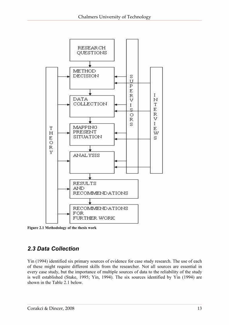
A case study is an empirical inquiry that investigates a contemporary phenomenon within its real-life context, especially when the boundaries between phenomenon and context are not clearly evident. The essence of a case study is that it tries to illuminate a decision or set of decisions: why they were taken, how they were implemented, and with which results. (Yin, 1994)
Case studies can be explanatory, exploratory and descriptive. Explanatory case studies is used to answer “how” and “why” questions. Exploratory case studies are used to explore and area which is not so much known. In descriptive case studies, the purpose is to describe a process or an event without analysis or value judgments. (Gummesson, 2003)
Later on, Stake (1995) included three others: Intrinsic, that is when the researcher has an interest in the case; Instrumental, when the case is used to understand more than what is obvious to the observer; Collective, when a group of cases is studied. Exploratory cases are sometimes considered as a prelude to social research. Explanatory case studies may be used for doing causal investigations. Descriptive cases require a descriptive theory to be developed before starting the project.
Case studies focus on understanding the dynamics present within a single setting. Yin (1994) presented four applications for a case study model:
1. To explain complex causal links in real-life interventions 2. To describe the real-life context in which the intervention has occurred 3. To describe the intervention itself 4. To explore those situations in which the intervention being evaluated has no clear set
of outcomes
For this thesis, an exploratory case study is carried out because a new method and its effects are under focus which is the specific case of implementing mixed load and smaller boxes for VPT’s inbound logistics. To achieve this aim, the methodology used can be seen in Figure 2.1 is followed.
Corakci & Dincer, 2008 12
Chalmers University of Technology
Figure 2.1 Methodology of the thesis work
2.3 Data Collection
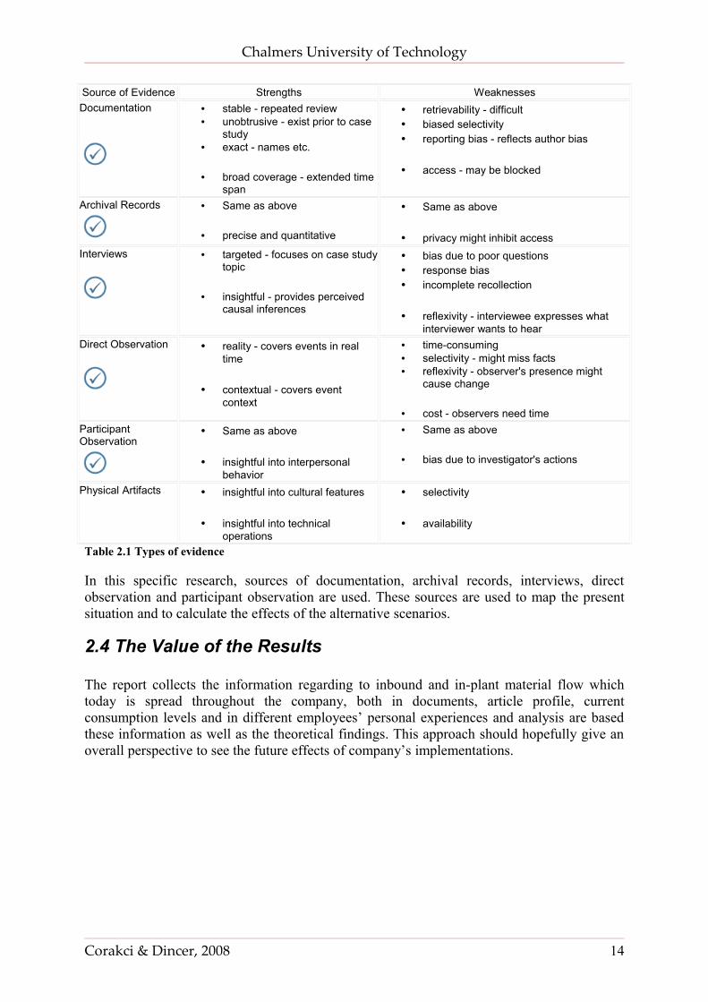
Yin (1994) identified six primary sources of evidence for case study research. The use of each of these might require different skills from the researcher. Not all sources are essential in every case study, but the importance of multiple sources of data to the reliability of the study is well established (Stake, 1995; Yin, 1994). The six sources identified by Yin (1994) are shown in the Table 2.1 below.
Corakci & Dincer, 2008 13
Chalmers University of Technology
Source of Evidence Strengths WeaknessesDocumentation • stable - repeated review
• unobtrusive - exist prior to case study
• exact - names etc.
• broad coverage - extended time span
• retrievability - difficult • biased selectivity • reporting bias - reflects author bias
• access - may be blocked
Archival Records • Same as above
• precise and quantitative
• Same as above
• privacy might inhibit access Interviews • targeted - focuses on case study
topic
• insightful - provides perceived causal inferences
• bias due to poor questions • response bias • incomplete recollection
• reflexivity - interviewee expresses what interviewer wants to hear
Direct Observation • reality - covers events in real time
• contextual - covers event context
• time-consuming • selectivity - might miss facts • reflexivity - observer's presence might
cause change
• cost - observers need time Participant Observation
• Same as above
• insightful into interpersonal behavior
• Same as above
• bias due to investigator's actions
Physical Artifacts • insightful into cultural features
• insightful into technical operations
• selectivity
• availability
Table 2.1 Types of evidence
In this specific research, sources of documentation, archival records, interviews, direct observation and participant observation are used. These sources are used to map the present situation and to calculate the effects of the alternative scenarios.
2.4 The Value of the Results
The report collects the information regarding to inbound and in-plant material flow which today is spread throughout the company, both in documents, article profile, current consumption levels and in different employees’ personal experiences and analysis are based these information as well as the theoretical findings. This approach should hopefully give an overall perspective to see the future effects of company’s implementations.
Corakci & Dincer, 2008 14
Chalmers University of Technology
3. THEORETICAL FRAMEWORK
This chapter explains the related works of literature for the thesis. This is thought to create a support for better understanding of the thesis for the people who are not up to date in the theories underlying this thesis.
3.1 Lean Thinking
Starting from 1980’s Japanese automotive manufacturers adopted the principle of lean thinking which refers to eliminating waste in all aspects of a business. Suffering shortages and lack of resources, Japanese manufacturers had to respond by developing new processes focusing on eliminating waste and these processes were not only limited to the production area but spreading from the shop floor to new product development and supply chain management. (Harrison, 2005)
Lean thinking got its name from a book called “The Machine That Changed the World: The Story of Lean Production” by Womack J.P. Jones D.T in 1990. The book was about the movement of automotive manufacturers from craft production to mass production to lean production. Then, Womack & Jones renewed the message of their previous book in “Lean Thinking” in 1996 and extended it beyond automotive industry. (Nicholas, 2006)
3.1.1 Principles of Lean Thinking
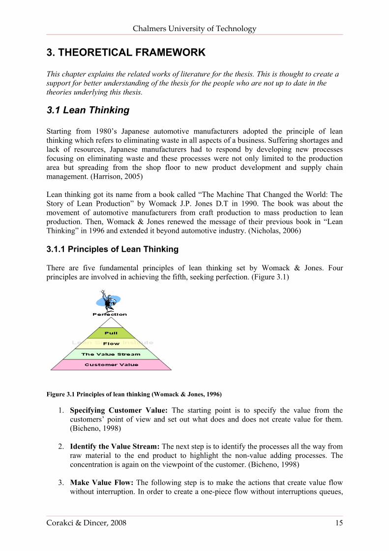
There are five fundamental principles of lean thinking set by Womack & Jones. Four principles are involved in achieving the fifth, seeking perfection. (Figure 3.1)
Figure 3.1 Principles of lean thinking (Womack & Jones, 1996)
1. Specifying Customer Value: The starting point is to specify the value from the customers’ point of view and set out what does and does not create value for them. (Bicheno, 1998)
2. Identify the Value Stream: The next step is to identify the processes all the way from raw material to the end product to highlight the non-value adding processes. The concentration is again on the viewpoint of the customer. (Bicheno, 1998)
3. Make Value Flow: The following step is to make the actions that create value flow without interruption. In order to create a one-piece flow without interruptions queues,
Corakci & Dincer, 2008 15
Chalmers University of Technology
delays, inventories, defects and downtime supports should be avoided or minimized. (Bicheno, 1998)
4. Pull Scheduling: Pull scheduling is about to produce only what is pulled by the customer. Pull can be in macro and micro levels. On the macro level, most companies have to push up to a certain level and response customers’ pull signals afterwards. The aim is to push this point further and further upstream. On the micro level, pull can come from the next station which is considered as an internal customer. (Bicheno, 1998)
5. Perfection: Perfection is the final point to reach. Perfection in lean thinking means producing exactly what the customer wants with no delay, at a fair price and with minimum waste. (Bicheno, 1998)
3.1.2 Waste Elimination in Lean Thinking
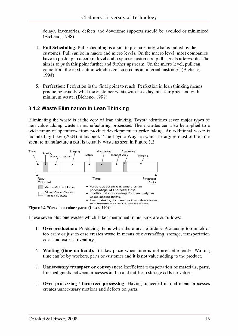
Eliminating the waste is at the core of lean thinking. Toyota identifies seven major types of non-value adding waste in manufacturing processes. These wastes can also be applied to a wide range of operations from product development to order taking. An additional waste is included by Liker (2004) in his book “The Toyota Way” in which he argues most of the time spent to manufacture a part is actually waste as seen in Figure 3.2.
Figure 3.2 Waste in a value system (Liker, 2004)
These seven plus one wastes which Liker mentioned in his book are as follows:
1. Overproduction: Producing items when there are no orders. Producing too much or too early or just in case creates waste in means of overstaffing, storage, transportation costs and excess inventory.
2. Waiting (time on hand): It takes place when time is not used efficiently. Waiting time can be by workers, parts or customer and it is not value adding to the product.
3. Unnecessary transport or conveyance: Inefficient transportation of materials, parts, finished goods between processes and in and out from storage adds no value.
4. Over processing / incorrect processing: Having unneeded or inefficient processes creates unnecessary motions and defects on parts.
Corakci & Dincer, 2008 16
Chalmers University of Technology
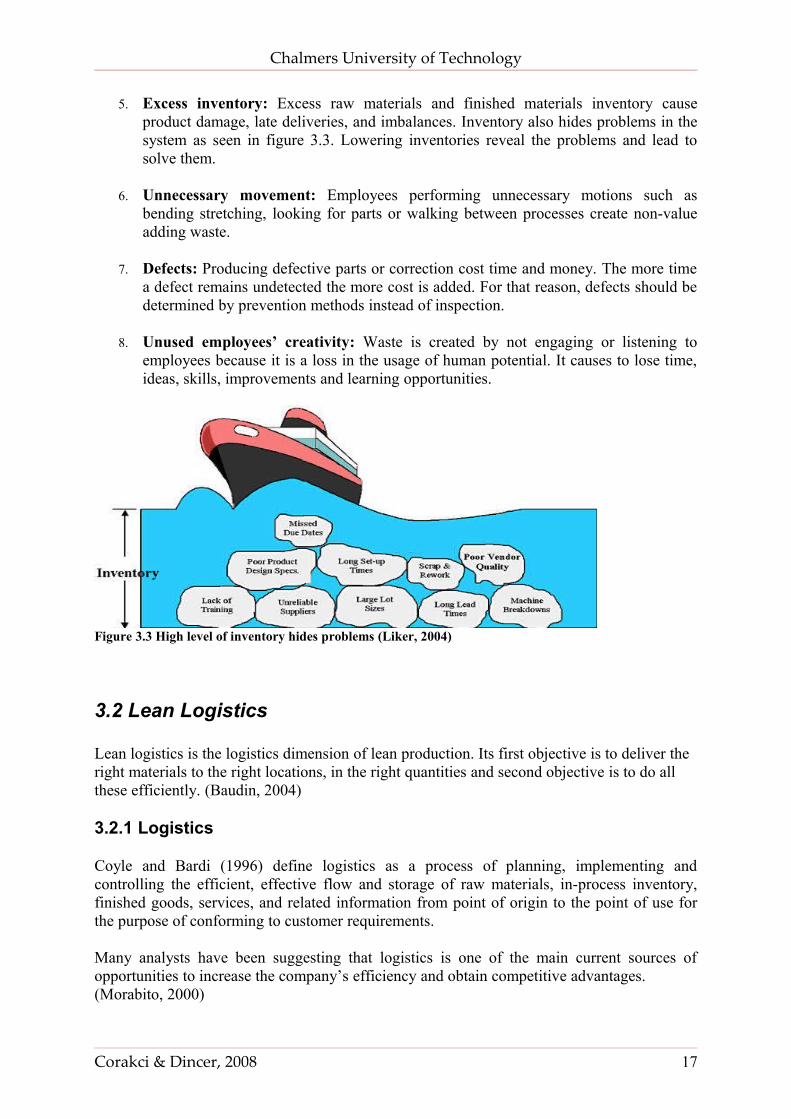
5. Excess inventory: Excess raw materials and finished materials inventory cause product damage, late deliveries, and imbalances. Inventory also hides problems in the system as seen in figure 3.3. Lowering inventories reveal the problems and lead to solve them.
6. Unnecessary movement: Employees performing unnecessary motions such as bending stretching, looking for parts or walking between processes create non-value adding waste.
7. Defects: Producing defective parts or correction cost time and money. The more time a defect remains undetected the more cost is added. For that reason, defects should be determined by prevention methods instead of inspection.
8. Unused employees’ creativity: Waste is created by not engaging or listening to employees because it is a loss in the usage of human potential. It causes to lose time, ideas, skills, improvements and learning opportunities.
Figure 3.3 High level of inventory hides problems (Liker, 2004)
3.2 Lean Logistics
Lean logistics is the logistics dimension of lean production. Its first objective is to deliver the right materials to the right locations, in the right quantities and second objective is to do all these efficiently. (Baudin, 2004)
3.2.1 Logistics
Coyle and Bardi (1996) define logistics as a process of planning, implementing and controlling the efficient, effective flow and storage of raw materials, in-process inventory, finished goods, services, and related information from point of origin to the point of use for the purpose of conforming to customer requirements.
Many analysts have been suggesting that logistics is one of the main current sources of opportunities to increase the company’s efficiency and obtain competitive advantages. (Morabito, 2000)
Corakci & Dincer, 2008 17
Chalmers University of Technology
Stock & Lambert (2001) mention multiple activities which are involved in the flow of products from point of origin to the point of use. These key logistics activities are listed as follows:
• Customer Service• Logistics communications• Demand Forecasting / Planning• Procurement• Warehousing and storage• Material handling• Inventory management• Order Processing• Packaging• Traffic and Transportation• Reverse Logistics• Return goods handling• Parts and service support • Plant and warehouse site selection
These logistics activities of a company are the major sources of waste if they are not organized efficiently. That is the reasoning behind the efforts to combine lean thinking with logistics. So, lean logistics includes all efforts in order to create a more effective and efficient logistics system by removing non-value adding activities and creating a one piece flow. (Baudin, 2004)
3.2.2 World Class Logistics
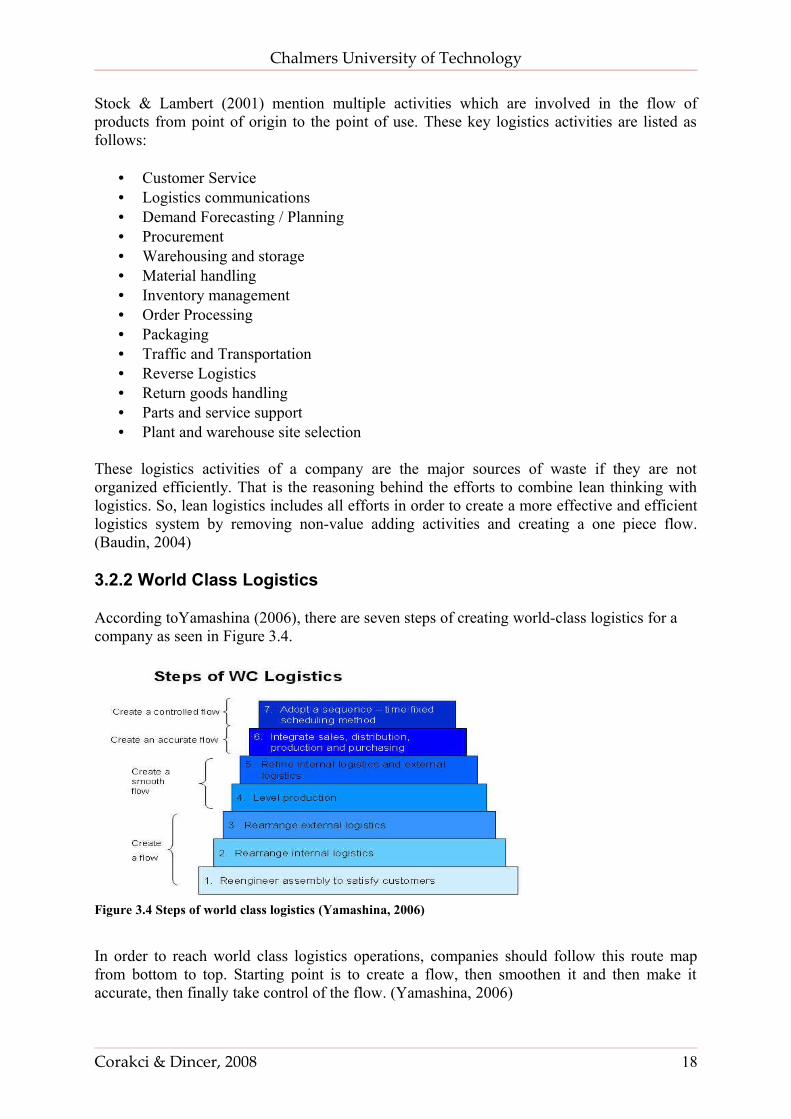
According toYamashina (2006), there are seven steps of creating world-class logistics for a company as seen in Figure 3.4.
Figure 3.4 Steps of world class logistics (Yamashina, 2006)
In order to reach world class logistics operations, companies should follow this route map from bottom to top. Starting point is to create a flow, then smoothen it and then make it accurate, then finally take control of the flow. (Yamashina, 2006)
Corakci & Dincer, 2008 18
Chalmers University of Technology
3.2.1 Inbound and outbound logistics
According to Baudin (2004), there are three main classifications of logistics:
• Inbound logistics• Outbound logistics• In–plant logistics
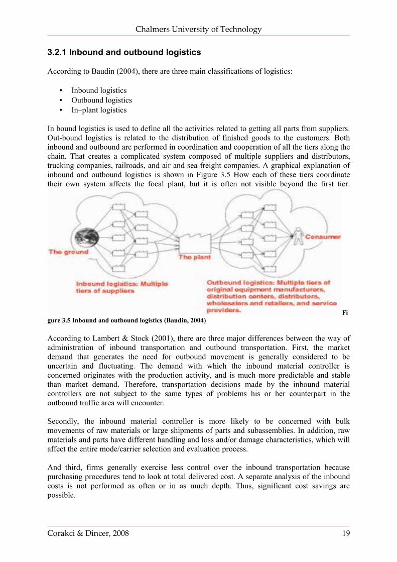
In bound logistics is used to define all the activities related to getting all parts from suppliers. Out-bound logistics is related to the distribution of finished goods to the customers. Both inbound and outbound are performed in coordination and cooperation of all the tiers along the chain. That creates a complicated system composed of multiple suppliers and distributors, trucking companies, railroads, and air and sea freight companies. A graphical explanation of inbound and outbound logistics is shown in Figure 3.5 How each of these tiers coordinate their own system affects the focal plant, but it is often not visible beyond the first tier.
Figure 3.5 Inbound and outbound logistics (Baudin, 2004)
According to Lambert & Stock (2001), there are three major differences between the way of administration of inbound transportation and outbound transportation. First, the market demand that generates the need for outbound movement is generally considered to be uncertain and fluctuating. The demand with which the inbound material controller is concerned originates with the production activity, and is much more predictable and stable than market demand. Therefore, transportation decisions made by the inbound material controllers are not subject to the same types of problems his or her counterpart in the outbound traffic area will encounter.
Secondly, the inbound material controller is more likely to be concerned with bulk movements of raw materials or large shipments of parts and subassemblies. In addition, raw materials and parts have different handling and loss and/or damage characteristics, which will affect the entire mode/carrier selection and evaluation process.
And third, firms generally exercise less control over the inbound transportation because purchasing procedures tend to look at total delivered cost. A separate analysis of the inbound costs is not performed as often or in as much depth. Thus, significant cost savings are possible.
Corakci & Dincer, 2008 19
Chalmers University of Technology
3.2.2 In - plant Logistics and Material Handling
Usually the tendency is not to call the activities within the plant as logistics but this term is used because there is a significant similarity between external logistics and what happens to material within the plant and besides, the elements inside the plant need to be integrated with the external system to be able visualize the process in a holistic fashion. (Management, 2008)
In-plant logistics is also called dock-to-dock logistics because it takes place in between the docks for receiving and shipping. Principally, for a company any activity that transforms materials in any way is production, not logistics. Still there is a thin boundary between production and logistics activities of a company and where this boundary is placed is a managerial decision. (Baudin, 2004)
Since the flow of materials is referred, transportation and material handling are two significant elements of it. (Management, 2008)
3.3 Material Flow Control
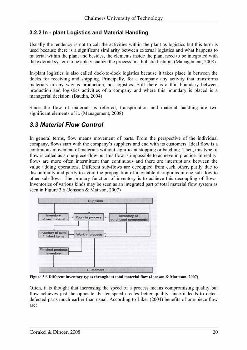
In general terms, flow means movement of parts. From the perspective of the individual company, flows start with the company’s suppliers and end with its customers. Ideal flow is a continuous movement of materials without significant stopping or batching. Then, this type of flow is called as a one-piece-flow but this flow is impossible to achieve in practice. In reality, flows are more often intermittent than continuous and there are interruptions between the value adding operations. Different sub-flows are decoupled from each other, partly due to discontinuity and partly to avoid the propagation of inevitable disruptions in one-sub flow to other sub-flows. The primary function of inventory is to achieve this decoupling of flows. Inventories of various kinds may be seen as an integrated part of total material flow system as seen in Figure 3.6 (Jonsson & Mattson, 2007)
Figure 3.6 Different inventory types throughout total material flow (Jonsson & Mattsson, 2007)
Often, it is thought that increasing the speed of a process means compromising quality but flow achieves just the opposite. Faster speed creates better quality since it leads to detect defected parts much earlier than usual. According to Liker (2004) benefits of one-piece flow are:
Corakci & Dincer, 2008 20
Chalmers University of Technology
1- Builds in Quality: In one piece flow, every operator is an inspector therefore it is much easier to detect and fix problems.
2- Creates Real Flexibility: Since the lead time to make a product is much shorter in a one-piece flow, there is more flexibility to respond and make what the customer really wants.
3- Creates Higher Productivity: In a one-piece flow cell, there is very little non-value added activity. It is very easy to see who is too busy and who is idle. It is also easy to calculate value added work in order to find how many employees are needed to reach a certain production rate.
4- Frees up Floor Space: In one-piece flow cell, everything is pushed close together and there is little space wasted by inventory.
5- Improves Safety: Since in a one-piece flow only smaller batches are transported in the factory, forklift trucks which are a major cause of accidents can be eliminated.
6- Improves Morale: In one-piece flow, people do much more value added work and can immediately see the results of that work, giving them both a sense of accomplishment and job satisfaction.
7- Reduces Cost of Inventory: In one-piece flow, WIP and finished goods inventory is minimized so the cost of inventory is significantly reduced.
3.3.1 Cycle Time and Takt Time
Cycle time is the time between when units are completed. The cycle time concept is thus important because it implies repetitiveness and smooth, steady flow of material throughout a process. Cycle time can also be thought as the inverse of production rate. For example, saying that a process has a cycle time of 10 minutes is almost the same thing as saying it has a production rate of six products per hour. (Nicholas, 1998)
Required cycle time (or takt time) is the production target of a process. It is determined by the demand. To satisfy demand, process should be designed in a way that actual cycle time does not exceed takt time. (Nicholas, 1998)
Liker (2004) states that takt time is the heart beat of one-piece flow. Takt is the rate at which customer is buying the product. In a true one-piece flow every step of the process should be producing exactly in the takt time. If they go faster there will be overproduction and if they go slower there will be bottleneck operations. Takt time can be used to set the pace of production and alert workers if they are going faster or slower.
3.3.2 Creating the one-piece flow
Creating a one-piece flow is difficult and there are two common mistakes done by companies. The first is that they set up fake flows. An example of fake flow is to move equipment close together to create a cell looks like a one-piece flow cell, but then batching the product at each stage with no sense of takt time. Therefore, it looks like a cell but works like a batch process. The second is that they go backwards from flow as soon as problems occur, which is called
Corakci & Dincer, 2008 21
Chalmers University of Technology
backtracking. This usually occur when a cost is related creating the flow, so companies tend to give up the flow. (Liker, 2004)
Setup time is the usual constraint which prevents the one-piece flow. Thus, to achieve the maximum benefits, it is crucial to minimize setup time. If setup time can be reduced to almost zero (or single minute) then it is possible to fill any sized order, regardless of product or quantity. As mentioned earlier, creating a one piece flow is at the core of lean thinking because it is very important to create the best quality at the lowest cost and in the shortest delivery time. One-piece flow also forces adoption of lean principles and practices such as preventive maintenance, poka-yoke, and other measures to eliminate waste and maximize quality. (Nicholas, 2006)
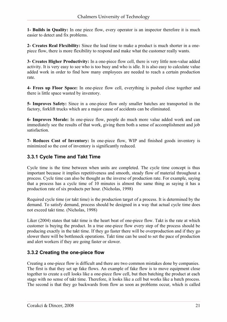
Point of use delivery is also used to remove non-value adding activities and create a one-piece flow. Point of use is the assembly station in a plant where the material is actually required. Point of use delivery means the materials are delivered directly to the assembly station without waiting in a warehouse. Figure 3.7 shows a plant which is divided into product-line focused factories. Each focused factory has its own receiving and shipping dock. (Nicholas, 2006)
Parts that are unique to each product line arrive at the receiving dock of the product’s focused factory and finished products depart at the shipping dock. Points of consumption are easy to find and interruptions to material flow are minimal because the plant is wide and with no walls. Parts that are used in more than one product line arrive at the dock in the center and are carted to the point of use. Incoming parts do not wait nor get stored. Steps for multiple handling are eliminated. Since the quality is guaranteed by the suppliers, there is no incoming inspection, either. (Nicholas, 2006)
Figure 3.7 Material flow in a plant with several focused factories (Nicholas, 2006)
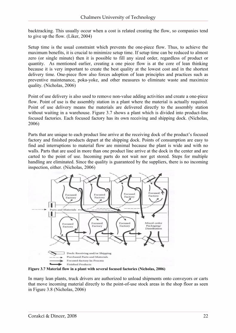
In many lean plants, truck drivers are authorized to unload shipments onto conveyors or carts that move incoming material directly to the point-of-use stock areas in the shop floor as seen in Figure 3.8 (Nicholas, 2006)
Corakci & Dincer, 2008 22
Chalmers University of Technology
A truck driver who is familiar with customer’s facility layout and procedures is a potential source of suggestions about how supplier might improve its service, or how the customer might take better advantage of that service. Partnering with the suppliers supports interaction in the opposite way, too. Associates from the customer plant meet their counterparts in the supplier’s shop and see how the parts they use are produced. (Nicholas, 2006)
Figure 3.8 Point- of-Use Delivery (Nicholas, 2006)
3.4 Packaging Logistics
Packaging Logistics is aiming at developing packaging and packaging systems that support the objectives of logistics to plan, implement and control the efficient and effective materials flow. (Johansson, 1997)
The packaging logistics approach includes the whole supply chain, from raw material producer to the end user, and the disposal of empty package. This means that all packaging levels are included in the approach. Furthermore, it is of great importance not to forget the product and the surrounding distribution system. In order not to sub optimize, product, packaging and distribution system should be seen as interactive parts. (Johansson, 2000)
3.4.1 Demands on Packaging
The shortcomings of many material-flow systems are increasingly under scrutiny, partly because of increased focus on the time factor. Demands on packaging differ in different parts of the material flow, and inability to meet these requirements often results in increased cost and delays. Repacking might be necessary, causing extra costs in labor and administration, as well as delaying the goods’ arrival at the next link in the chain. Since the material flow continues in the next production phase, it is just as important that the packaging works at the receiving end without unnecessary repacking or handling. In order to achieve high efficiency material flow, it is important for packaging to be adapted to the emptying / unpacking process at the receiving end as to the filling / packing process at the supplying end. (Torstensson, 2006)
Volume Efficiency
High volume utilization is important in order to be efficient in economical terms. The volume utilization of packaging can be considered in two levels: internal and external filling degree.
Corakci & Dincer, 2008 23
Chalmers University of Technology
Internal filling degree of the packaging depends mainly on product shape, design and lining. When using standardized packaging with fixed sizes, the internal filling degree might not always be optimal. The external filling degree of packaging is related to adaptation to modular standards as regards measures and stacking heights. To reach optimal volume efficiency, both of these levels must be taken into consideration by applying an overall view on three factors which are: product, packaging and distribution environment. (Johansson, 1997)
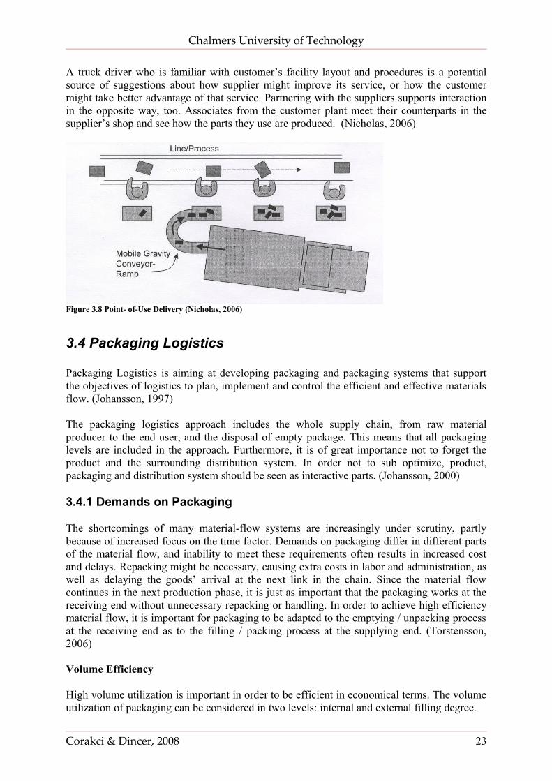
It is important for empty packaging to be volume efficient too. Empty packaging that are stackable or can be compressed in some other way save space when transported and in the storage area as seen in Figure 3.9.
Figure 3.9 Standardized packages (Yamashina, 2006)
Weight Efficiency
Generally there is a demand that a packaging should weight as little as possible. The amount of good that can be transported on a load carrier is limited as to weight and volume.
The weight of packaging is particularly important when manual handling is part of the material flow. There is a risk of personal injury when lifting more than 75 kg for men and 45 kg for women, but lifting may already be a hazard at 20 kg for men and 12 kg for women. The extent of the risk will depend on posture, range of lifting and frequency of lifting. A general maximum value used for low frequent lifts in Sweden is 15 kg. (Torstensson, 2006)
Process Integration
Packing / filling and handling of the packaging should be regarded as an integrated part of production. This means handling operations shall be as few as possible and be easy and fast to perform. Such a packaging should be adapted to different operations at erecting, filling, sealing, labeling and palletizing. It is also important if the handling is manual or automatic. Generally, automatic handling demands more accurate tolerances and higher repeatability. Manual handling is more tolerant to variations in the packaging. (Johansson, 2000)
Handleability
The packaging must be easy to handle all kinds of conditions that occurs on its way through supply chain so that there will not occur a need for repacking. Johansson (2000) states that handleability can be measured from three aspects:
• Time: how long a certain activity takes
Corakci & Dincer, 2008 24
Chalmers University of Technology
• Force: the force needed for a certain activity• Instruction: information about how to best perform a certain activity
Deficiency in handleability affects both manual and automatic handling and will have an economic impact regarding: Work load disorders, product damage due to incorrect handling, increased machinery cost and customer rejection of a product. (Johansson, 2000)
3.4.2 Mixed Load
Mixed Load palletizing is one of the identified methods that reduce costs and streamline thesupply chain. As manufacturers change how they produce and distribute their products, mixed load palletizing emerges as one of the most efficient technologies companies can implement. In general, mixed load palletizing is a mindset bringing the manufacturing and distribution environment closer together to review the complete supply-chain process to identify savings in labor, floor space and inventory.
Teulings & Vlist (2001) suggest that especially for low value parts, mixed loading can be very efficient. By synchronizing replenishment periods of different parts, handling can be reduced and resources and cost of information can be shared.
Balintfy (1964) describes an approach for inventory management that is when a part is needed to be replenished and looks for more combinations with other parts that are also almost needed to be replenished. As a result of this approach loading devices (packages, pallets) contain a customer-specific mixed load. From an inventory point of view, this activity should be placed as far downstream as possible in the supply chain so that the stock requirements will be minimized. On the other hand, from a handling point of view mixed load should be placed as far upstream as possible in the supply chain so that downstream stages will only handle larger mixed loads which will reduce the handling.
To be able to become familiar with mixed load palletizing technology, one needs to understand the software advances allowing mixed load palletizing to become a cost-effective reality. There exist two general types of palletizing software:
1. Software that builds planned pallet loads 2. Software capable of building random pallet loads
The two differ in that planned-pallet load software needs to know the location or identity of the product before it reaches the palletizer, while random-palletizing software can build mixed loads on the fly. Planned software can build a traditional homogeneous pallet (pure load) or a rainbow mixed pallet load where different layers of the pallet are created out of different products. A rainbow pallet for example might involve a pallet built from varying layers of beverages: the base being cola, the next level being diet, and the third, lemon-lime. From the side, the pallet would resemble a rainbow.
The benefit of a planned rainbow or pure load pallet is the high degree of pallet density. The disadvantage is that rainbow and homogeneous pallets don’t allow for the flexibility of building custom pallets to specific customer orders like mixed loads do.
To be able to enjoy the benefits of mixed loads, random pallet-building software had to be developed and evolved to a point where it was cost-effective to the company utilizing it.
Corakci & Dincer, 2008 25
Chalmers University of Technology
Random or mixed-pallet-building software permits robots or other flexible palletizing hardware to build pallets of products on the fly as they arrive at the palletizing cell.
Moreover, there are even some hardware differences. Planned pallets can utilize various type of equipment, from in feed and sorting conveyors to conventional and robotic palletizers. With the variety of hardware available, planned-palletizing cells tend to occupy more floor space than random-palletizing cells and often prove less flexible than their mixed-palletizing counterparts. Mixed-palletizing cells generally consist of less equipment, but at least two pieces are needed which are an infeed conveyor and a robotic palletizer. Both pieces utilize less floor space due to the hardware’s flexible layout.
3.5 Transportation
Transportation is one of the most significant areas of logistics management because its impact on customer service levels and firm’s cost structure. Inbound and outbound transportation costs can account for as much as 10 to 20 percent of product prices, sometimes even more. Effective management of transportation can result in significant improvements in profitability. (Cooke, 1993)
There is a continuously growing demand for fast and efficient transport. This is the reason why road transportation has increased significantly compared to other modes of transportation. Road transportation allows that larger quantities of goods such as more than one ton can be transported from door to door. The number of re-loadings can also be reduced which leads to decreasing costs and less damage on the goods. There are primarily two types of shipping: truckload (TL) and less-than-truckload (LTL). TL often gets a direct door-to-door service. Besides, TL shipments are large enough to fill up the entire truck and this in turn decreases the necessity for reloading and handling the goods during the transportation, thus minimizing costs for these operations, decreasing the risk for damages and shortening the transportation times. (Lumsden, 2002)
According to Yamashina (2006), there are three basic methods for external transportation of a company which are:
1. Direct Shipment2. Consolidation Center3. Mixed Transportation & Mixed Load (milk runs)
3.5.1 Direct Shipment
With this method, supply chain is structured in such a way that all shipments come directly from the suppliers to the company. With a direct shipment network the routing of each shipment is specified and the supply chain manager has nothing to decide about except the quantity of parts and mode of transportation.
The major advantage of a direct transportation network is the elimination of the intermediate warehouses and its simplicity of operation and coordination. The shipment decision is completely local and the decision made for one shipment does not affect others.
Corakci & Dincer, 2008 26
Chalmers University of Technology
A direct shipment network is justified if the supplier has enough capacity to send a TL. However, with smaller suppliers direct transportation network tends to have higher cost. If a TL carrier is used for each supplier, then the inventory level and the related costs will increase. On the other hand, if LTL is used transportation cost will increase. In direct shipment network, receiving costs are extremely high because each supplier should make a separate delivery.
3.5.2 Consolidation Center
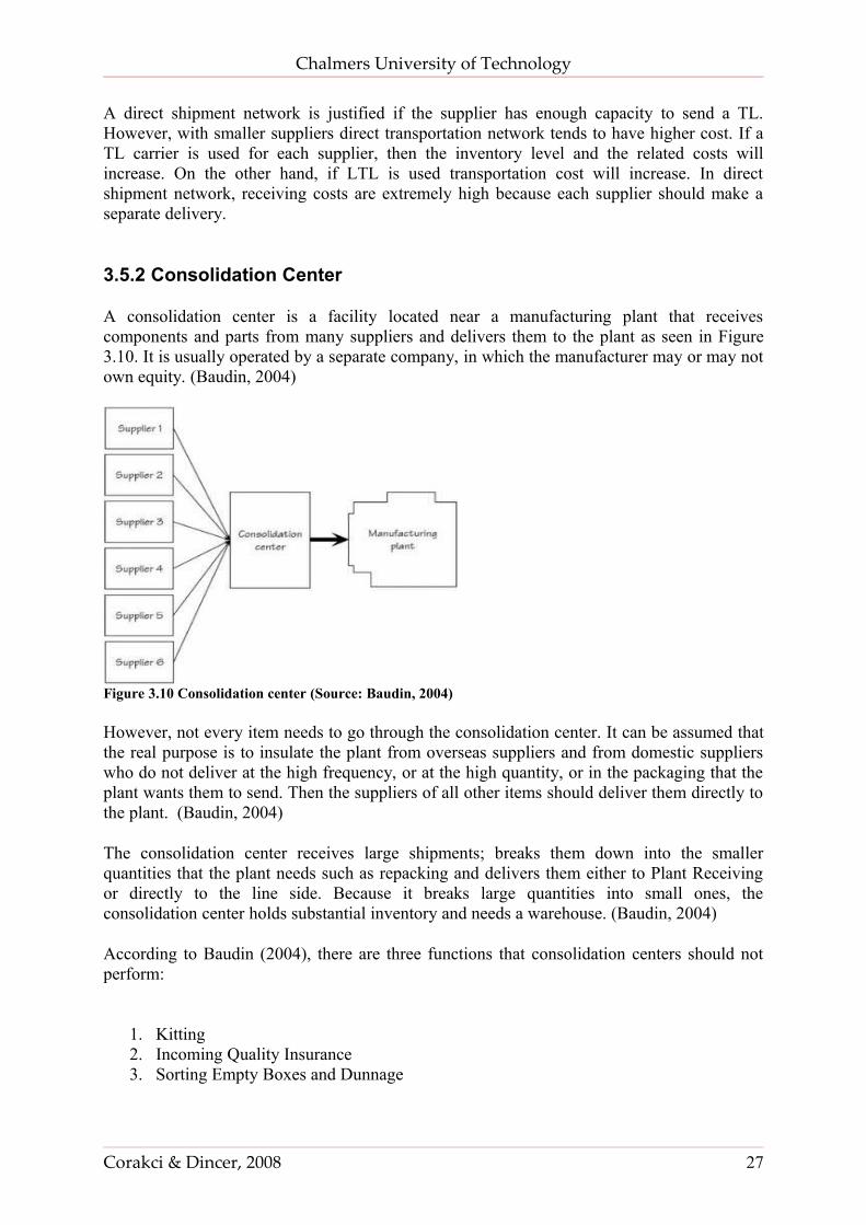
A consolidation center is a facility located near a manufacturing plant that receives components and parts from many suppliers and delivers them to the plant as seen in Figure 3.10. It is usually operated by a separate company, in which the manufacturer may or may not own equity. (Baudin, 2004)
Figure 3.10 Consolidation center (Source: Baudin, 2004)
However, not every item needs to go through the consolidation center. It can be assumed that the real purpose is to insulate the plant from overseas suppliers and from domestic suppliers who do not deliver at the high frequency, or at the high quantity, or in the packaging that the plant wants them to send. Then the suppliers of all other items should deliver them directly to the plant. (Baudin, 2004)
The consolidation center receives large shipments; breaks them down into the smaller quantities that the plant needs such as repacking and delivers them either to Plant Receiving or directly to the line side. Because it breaks large quantities into small ones, the consolidation center holds substantial inventory and needs a warehouse. (Baudin, 2004)
According to Baudin (2004), there are three functions that consolidation centers should not perform:
1. Kitting2. Incoming Quality Insurance3. Sorting Empty Boxes and Dunnage
Corakci & Dincer, 2008 27
Chalmers University of Technology
3.5.2.1 ABC Classification
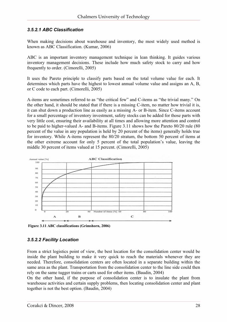
When making decisions about warehouse and inventory, the most widely used method is known as ABC Classification. (Kumar, 2006)
ABC is an important inventory management technique in lean thinking. It guides various inventory management decisions. These include how much safety stock to carry and how frequently to order. (Cimorelli, 2005)
It uses the Pareto principle to classify parts based on the total volume value for each. It determines which parts have the highest to lowest annual volume value and assigns an A, B, or C code to each part. (Cimorelli, 2005)
A-items are sometimes referred to as “the critical few” and C-items as “the trivial many.” On the other hand, it should be stated that if there is a missing C-item, no matter how trivial it is, it can shut down a production line as easily as a missing A- or B-item. Since C-items account for a small percentage of inventory investment, safety stocks can be added for those parts with very little cost, ensuring their availability at all times and allowing more attention and control to be paid to higher-valued A- and B-items. Figure 3.11 shows how the Pareto 80/20 rule (80 percent of the value in any population is held by 20 percent of the items) generally holds true for inventory. While A-items represent the 80/20 stratum, the bottom 50 percent of items at the other extreme account for only 5 percent of the total population’s value, leaving the middle 30 percent of items valued at 15 percent. (Cimorelli, 2005)
Figure 3.11 ABC classifications (Grimshorn, 2006)
3.5.2.2 Facility Location
From a strict logistics point of view, the best location for the consolidation center would be inside the plant building to make it very quick to reach the materials whenever they are needed. Therefore, consolidation centers are often located in a separate building within the same area as the plant. Transportation from the consolidation center to the line side could then rely on the same tugger trains or carts used for other items. (Baudin, 2004)On the other hand, if the purpose of consolidation center is to insulate the plant from warehouse activities and certain supply problems, then locating consolidation center and plant together is not the best option. (Baudin, 2004)
Corakci & Dincer, 2008 28
Chalmers University of Technology
Center of Gravity Technique
The center of gravity technique can be used to make decision about the location of a terminal or warehouse when multiple suppliers or customer bases exist at different geographic locations in order to supply all of them in the most economical way. (Mills, 2008)
In general, transportation costs are a function of distance, weight, and time. The center of gravity technique is a quantitative method for locating a facility, such as a warehouse, in this context the consolidation center, at the center of movement in a geographic area, based on weight and distance. (Mills, 2008)
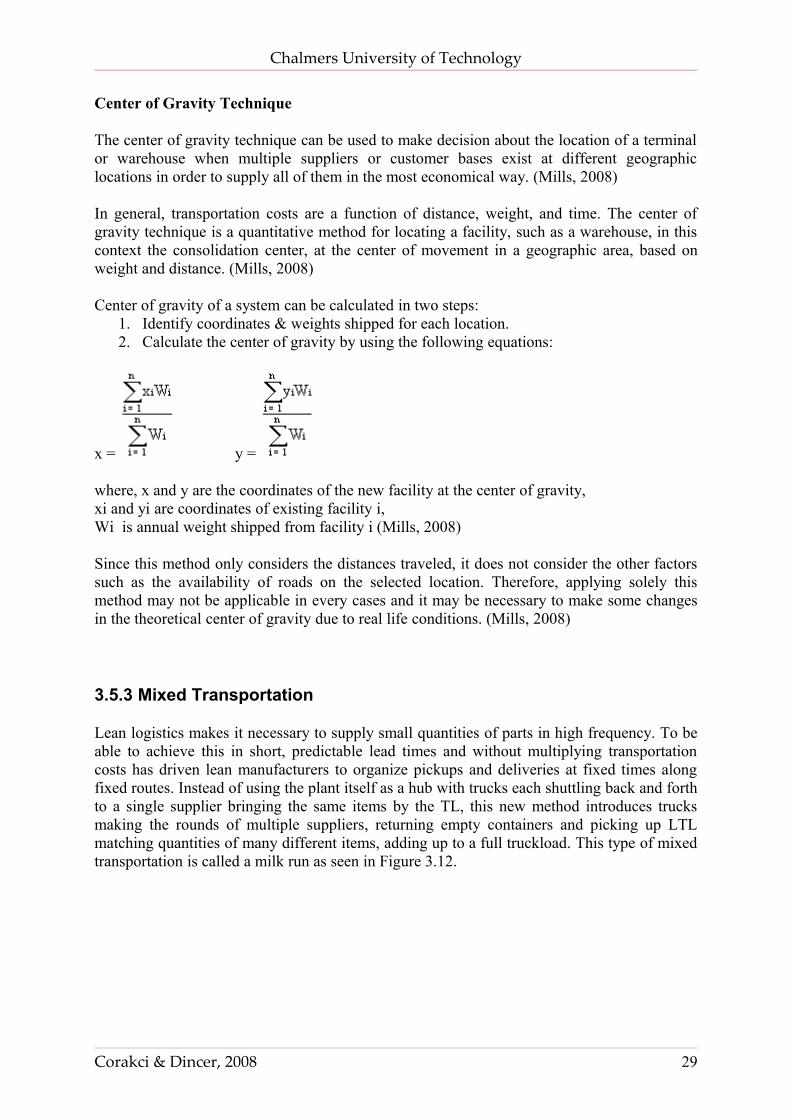
Center of gravity of a system can be calculated in two steps:1. Identify coordinates & weights shipped for each location.2. Calculate the center of gravity by using the following equations:
x = y =
where, x and y are the coordinates of the new facility at the center of gravity,xi and yi are coordinates of existing facility i, Wi is annual weight shipped from facility i (Mills, 2008)
Since this method only considers the distances traveled, it does not consider the other factors such as the availability of roads on the selected location. Therefore, applying solely this method may not be applicable in every cases and it may be necessary to make some changes in the theoretical center of gravity due to real life conditions. (Mills, 2008)
3.5.3 Mixed Transportation
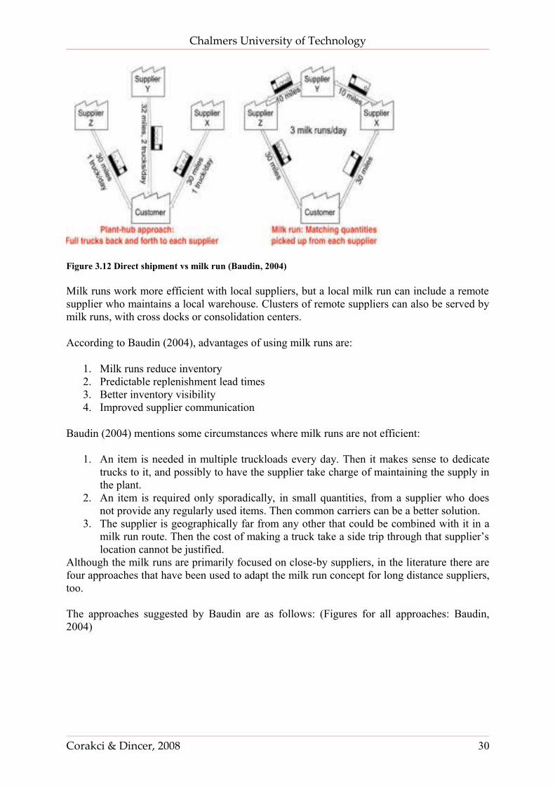
Lean logistics makes it necessary to supply small quantities of parts in high frequency. To be able to achieve this in short, predictable lead times and without multiplying transportation costs has driven lean manufacturers to organize pickups and deliveries at fixed times along fixed routes. Instead of using the plant itself as a hub with trucks each shuttling back and forth to a single supplier bringing the same items by the TL, this new method introduces trucks making the rounds of multiple suppliers, returning empty containers and picking up LTL matching quantities of many different items, adding up to a full truckload. This type of mixed transportation is called a milk run as seen in Figure 3.12.
Corakci & Dincer, 2008 29
Chalmers University of Technology
Figure 3.12 Direct shipment vs milk run (Baudin, 2004)
Milk runs work more efficient with local suppliers, but a local milk run can include a remote supplier who maintains a local warehouse. Clusters of remote suppliers can also be served by milk runs, with cross docks or consolidation centers.
According to Baudin (2004), advantages of using milk runs are:
1. Milk runs reduce inventory2. Predictable replenishment lead times3. Better inventory visibility4. Improved supplier communication
Baudin (2004) mentions some circumstances where milk runs are not efficient:
1. An item is needed in multiple truckloads every day. Then it makes sense to dedicate trucks to it, and possibly to have the supplier take charge of maintaining the supply in the plant.
2. An item is required only sporadically, in small quantities, from a supplier who does not provide any regularly used items. Then common carriers can be a better solution.
3. The supplier is geographically far from any other that could be combined with it in a milk run route. Then the cost of making a truck take a side trip through that supplier’s location cannot be justified.
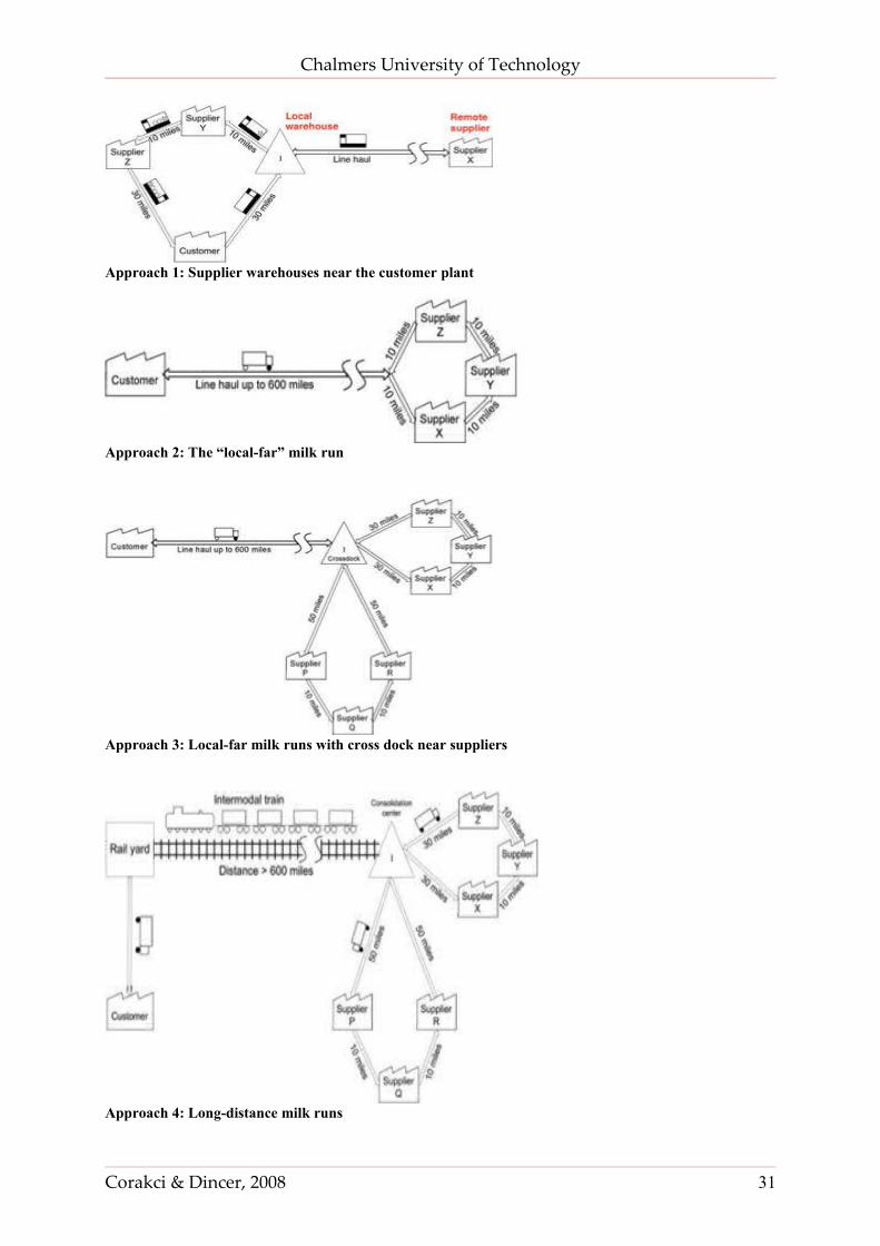
Although the milk runs are primarily focused on close-by suppliers, in the literature there are four approaches that have been used to adapt the milk run concept for long distance suppliers, too.
The approaches suggested by Baudin are as follows: (Figures for all approaches: Baudin, 2004)
Corakci & Dincer, 2008 30
Chalmers University of Technology
Approach 1: Supplier warehouses near the customer plant
Approach 2: The “local-far” milk run
Approach 3: Local-far milk runs with cross dock near suppliers
Approach 4: Long-distance milk runs
Corakci & Dincer, 2008 31
Chalmers University of Technology
3.6 Transportation Cost
Transportation cost is not easy to estimate and there exists several approaches in the literature to have a better estimation of the transportation cost.
3.6.1 Transportation Cost Structure
Transportation cost can be classified into following categories:
Fixed Cost
Fixed cost is the expenses that do not change in the short run and must be serviced even when a company is not operating. It includes costs which are not directly proportional to shipment volume. For transportation firms, fixed components include vehicles, terminals, information systems and support equipment. In the short term, expenses associated with fixed assets must be covered by contribution above variable costs on a per shipment basis. (Stock, 2001)
Variable Cost
Variable cost changes in a predictable manner in relation to some level of activity. Variable cost can only be avoided by not operating the vehicle. The variable category includes direct carrier cost associated with movement of each load. This cost is generally measured as cost per kilometer or per unit of weight. Typical variable cost components include driver’s wage, fuel and maintenance. (Stock, 2001)
Common Cost
Common cost includes carrier costs that are incurred on behalf of all or selected shippers. Terminal costs and management expenses are typical examples of common costs and are often allocated to a shipper according to a level of activity like the number of shipments or deliveries handled. (Stock, 2001)
Joint Cost
Joint cost is the expenses that are directly created by a decision to provide a particular service. Joint costs have significant impact on transportation charges because carrier quotations must include joint costs based on considerations regarding an appropriate backhaul shipper and/or charges against the original shipper. (Stock, 2001)
3.6.2 Transportation Cost Parameters
Transportation costs are driven by several factors. Even though each factor is not a direct component of transport tariffs as itself, it influences rates. These factors are:
Distance
Distance directly contributes to variable costs, such as fuel, labor and maintenance. The relationship between distance and cost is shown in Figure 3.13. The curve does not begin at zero cost for distance zero due to fixed costs of transportation. Fixed costs are independent of
Corakci & Dincer, 2008 32
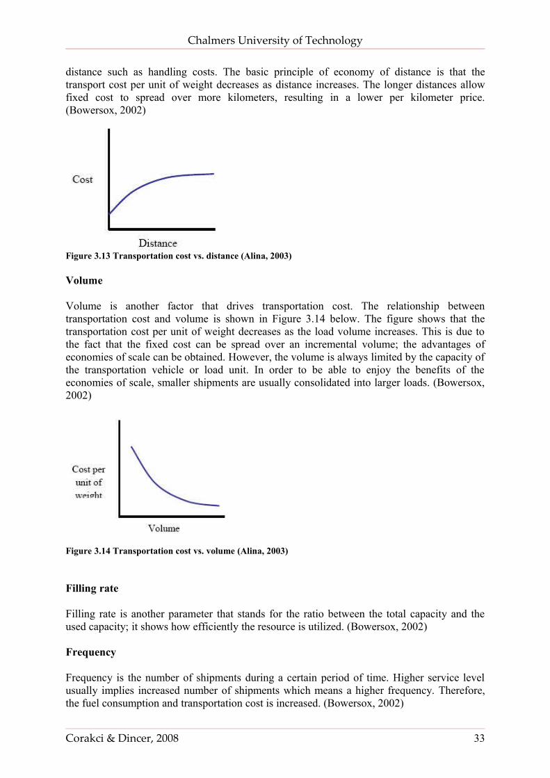
Chalmers University of Technology
distance such as handling costs. The basic principle of economy of distance is that the transport cost per unit of weight decreases as distance increases. The longer distances allow fixed cost to spread over more kilometers, resulting in a lower per kilometer price. (Bowersox, 2002)
Figure 3.13 Transportation cost vs. distance (Alina, 2003)
Volume
Volume is another factor that drives transportation cost. The relationship between transportation cost and volume is shown in Figure 3.14 below. The figure shows that the transportation cost per unit of weight decreases as the load volume increases. This is due to the fact that the fixed cost can be spread over an incremental volume; the advantages of economies of scale can be obtained. However, the volume is always limited by the capacity of the transportation vehicle or load unit. In order to be able to enjoy the benefits of the economies of scale, smaller shipments are usually consolidated into larger loads. (Bowersox, 2002)
Figure 3.14 Transportation cost vs. volume (Alina, 2003)
Filling rate
Filling rate is another parameter that stands for the ratio between the total capacity and the used capacity; it shows how efficiently the resource is utilized. (Bowersox, 2002)
Frequency
Frequency is the number of shipments during a certain period of time. Higher service level usually implies increased number of shipments which means a higher frequency. Therefore, the fuel consumption and transportation cost is increased. (Bowersox, 2002)
Corakci & Dincer, 2008 33
Chalmers University of Technology
Stowability
Stowability is the ability of the dimension of the parts to fit into transportation equipment, for example into a truck. If the goods are unusual in shape, size or weight, then it could be difficult to load and space into the transportation equipment. Since the volume cannot be utilized in the most efficient way, filling rate decreases and the transportation cost increases.(Bowersox, 2002)
Handling
Handling of the parts affects the transportation cost, too. If the transport requires special handling equipment, the transportation cost increases. (Bowersox, 2002)
The Choice of Transport Mode
The choice of transportation mode is affected by the nature of transported parts, infrastructure, service level required, lead-time aspect, etc. Therefore, the choice of transport mode directly affects the transportation cost. (Bowersox, 2002)
3.6.3 Road Transportation
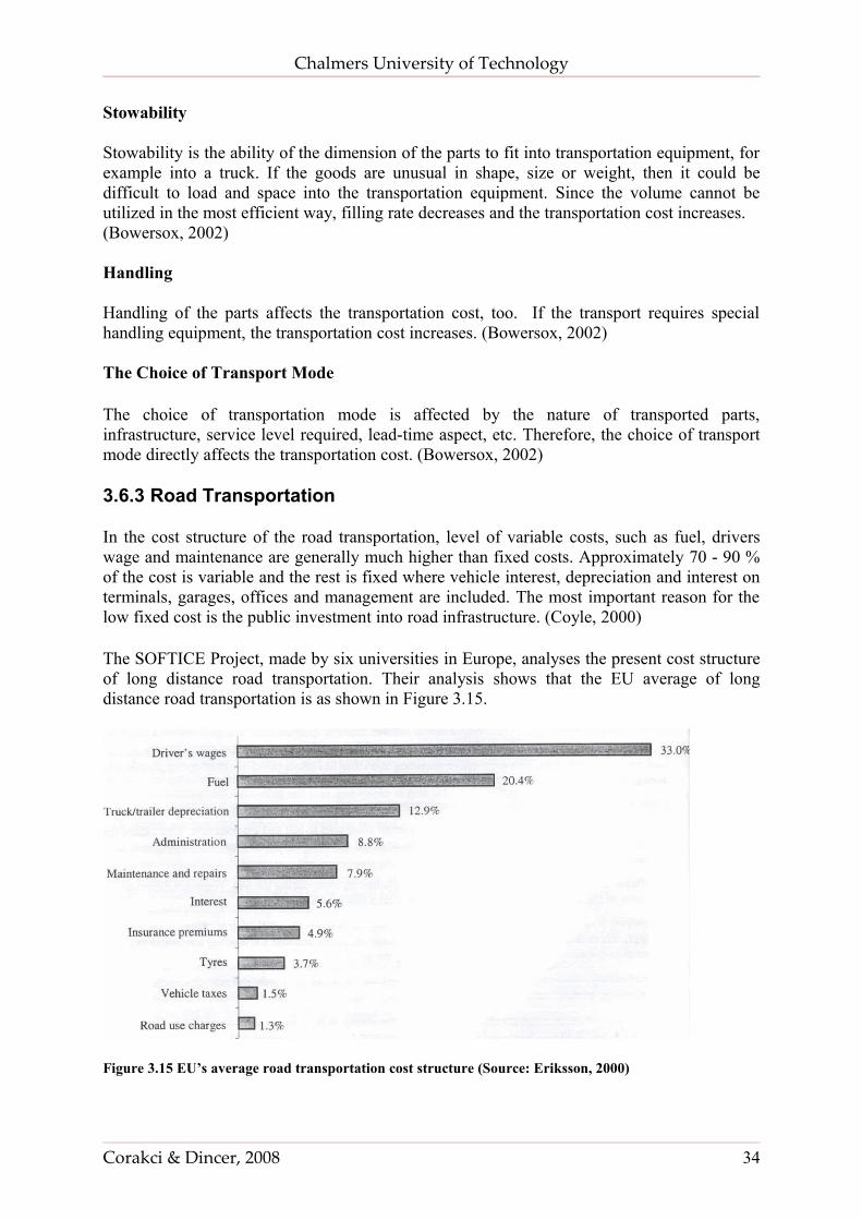
In the cost structure of the road transportation, level of variable costs, such as fuel, drivers wage and maintenance are generally much higher than fixed costs. Approximately 70 - 90 % of the cost is variable and the rest is fixed where vehicle interest, depreciation and interest on terminals, garages, offices and management are included. The most important reason for the low fixed cost is the public investment into road infrastructure. (Coyle, 2000)
The SOFTICE Project, made by six universities in Europe, analyses the present cost structure of long distance road transportation. Their analysis shows that the EU average of long distance road transportation is as shown in Figure 3.15.
Figure 3.15 EU’s average road transportation cost structure (Source: Eriksson, 2000)
Corakci & Dincer, 2008 34
Chalmers University of Technology
3.7 Supplier Relations
From the supplier’s point of view, manufacturers are customers. Therefore, suppliers should guarantee delivery on time with the right quantity and quality. To achieve this, efforts should be devoted to develop a smooth material flow from supplier to manufacturer. (Suzaki, 1987)
A lean supplier network should have the following characteristics:
1. A small number of direct suppliers with a tier structure: Lean manufacturers rely on a tier structure allowing each large supplier to manage a group of smaller ones.
2. Single-sourcing: Lean manufacturers do not use the strategy of sourcing the same item from multiple suppliers to assure supply.
3. Collaboration in product design: The more complex a manufactured product is, the less sense it makes to treat its components like commodities. Instead, they are specific to the product and designed for it.
4. Collaboration in cost reduction during production: During production, supplier and customer work together to reduce costs.
5. Collaboration in problem-solving and emergency response: Lean manufacturers do not look for suppliers who “never have any problems” but for suppliers who don’t hide them
6. A community: The suppliers of a lean manufacturer are an organized community. For example: Suppliers to NUMMI, which is a joint venture between General Motors and Toyota to build vehicles in the United States, should participate in GAMA (Golden State Automotive Manufacturers Association) (Baudin, 2004)
3.7.1 Vendor Managed Inventory (VMI)
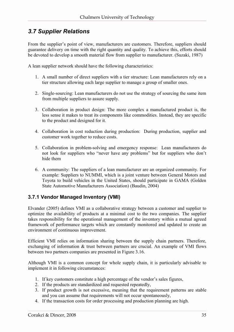
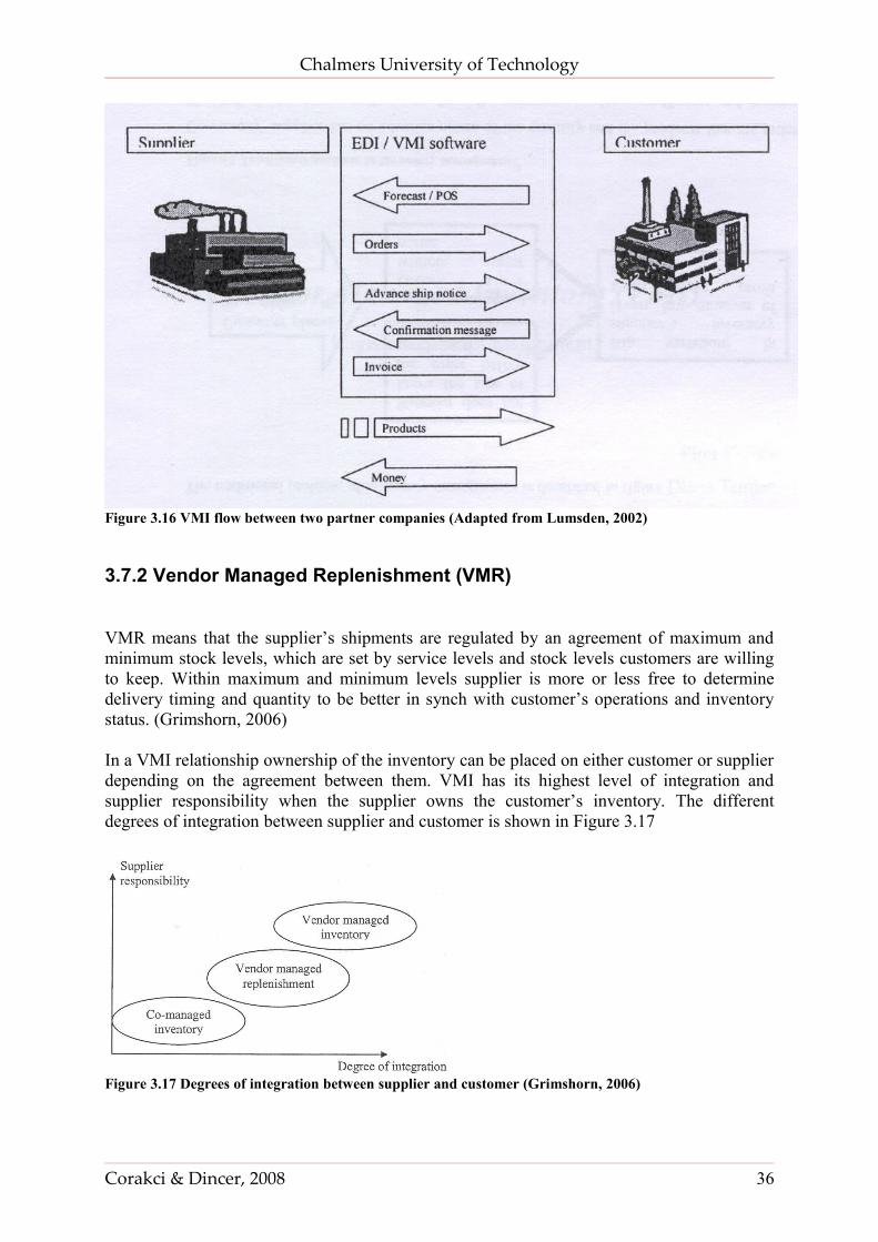
Elvander (2005) defines VMI as a collaborative strategy between a customer and supplier to optimize the availability of products at a minimal cost to the two companies. The supplier takes responsibility for the operational management of the inventory within a mutual agreed framework of performance targets which are constantly monitored and updated to create an environment of continuous improvement.
Efficient VMI relies on information sharing between the supply chain partners. Therefore, exchanging of information & trust between partners are crucial. An example of VMI flows between two partners companies are presented in Figure 3.16.
Although VMI is a common concept for whole supply chain, it is particularly advisable to implement it in following circumstances:
1. If key customers constitute a high percentage of the vendor’s sales figures,2. If the products are standardized and requested repeatedly,3. If product growth is not excessive, meaning that the requirement patterns are stable
and you can assume that requirements will not occur spontaneously, 4. If the transaction costs for order processing and production planning are high.
Corakci & Dincer, 2008 35
Chalmers University of Technology
Figure 3.16 VMI flow between two partner companies (Adapted from Lumsden, 2002)
3.7.2 Vendor Managed Replenishment (VMR)
VMR means that the supplier’s shipments are regulated by an agreement of maximum and minimum stock levels, which are set by service levels and stock levels customers are willing to keep. Within maximum and minimum levels supplier is more or less free to determine delivery timing and quantity to be better in synch with customer’s operations and inventory status. (Grimshorn, 2006)
In a VMI relationship ownership of the inventory can be placed on either customer or supplier depending on the agreement between them. VMI has its highest level of integration and supplier responsibility when the supplier owns the customer’s inventory. The different degrees of integration between supplier and customer is shown in Figure 3.17
Figure 3.17 Degrees of integration between supplier and customer (Grimshorn, 2006)
Corakci & Dincer, 2008 36

Chalmers University of Technology
4. PRESENT SITUATION
In order to have a successful improvement in the system, it is significant to know how the existing processes works today. This chapter presents observations made during the work and as well as analysis of the present system.
4.1 Packaging and Mixed Load
There are more than 6000 articles being used at VPT, from small gaskets, rings, nuts, bolts and screws to huge cylinder blocks, housing and flywheel assemblies. For holding this variety of articles Volvo’s own designed packages of different sizes are used. Among the available package types the most appropriate one is assigned to the article according to its weight, dimension and consumption level. Since Lean Assembly Line project has picked up it s speed, smaller packages are started to be preferred as much as possible to support the project. However, according to Håkan Sundberg, supplier’s current packaging equipment is also an issue which even leads compromises of using unwanted and unstandardized package types.
In the following section current packaging of VPT’s articles are investigated further for both in-plant and inbound material flow. However only 70% of these articles are purchased and are in the scope of this study. Purchased articles make up 50% of the yearly value of total articles.
4.1.1 Packaging
The articles are mostly carried inside pallets from suppliers to VPT. However smallest holding unit of them are not always the pallets in the plant. 100-cartoon, 156-cartoon, 750-plastic and 780-plastic boxes are the 4 main inner packages that are carried inside pallets and used at point of use to expose articles. Other than these, plastic bags, some supplier specific packages and 2 other different sizes of cartoon packages are used in less frequently basis. As well as these inner packages; K,L,H,F and G types of pallets and combitainers are also directly used as the smallest holding unit at the assembly. Dimensions, weight and price of these packages are given in the Appendix A. It is difficult to create an exactly accurate profile of current package used in the inbound flow since data extracted from the VPT’s system was not complete. That’s why, some primary data collection was held in the assembly area for the purpose of reaching to a higher level of current packaging data of articles. Final collection results covers 96% of total yearly volume value and 98% of total yearly weight but only 79% of total count of articles as it is given at the Table 4.1 below.
Total Yearly Weight (kg)
Total Yearly Volume Value (sek)
Total Count of Articles
Articles with known current smallest holding unit 67731064 XXXXX 3316Whole purchased articles 68870140 XXXXX 4222Data collection scope 98% 96% 79%Table 4.1 Data collection scope of current smallest holding unit
The reason of having low ratio on “total count of articles” is the low accessibility of C-Volume articles which constitutes small fraction of the total yearly volume but relatively high fraction of total count of articles. Below at Table 4.2 the total yearly volume value and cumulative weight of class types are listed. Since the collected data is only for the purchased
Corakci & Dincer, 2008 37
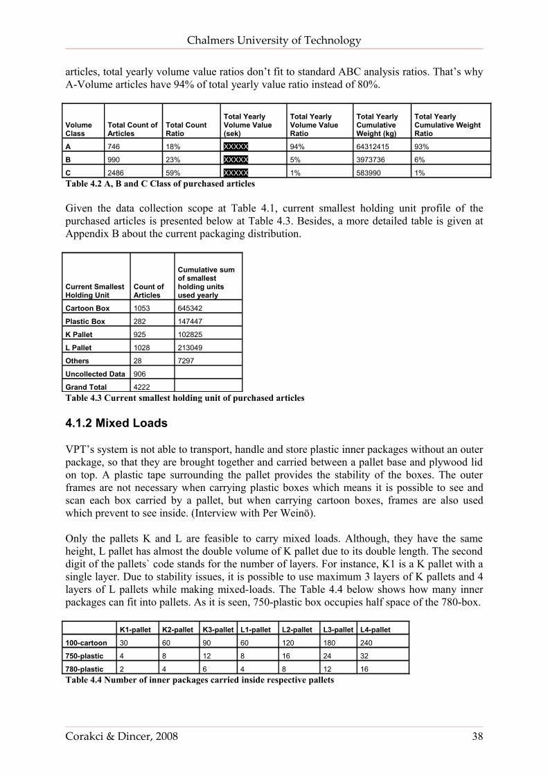
Chalmers University of Technology
articles, total yearly volume value ratios don’t fit to standard ABC analysis ratios. That’s why A-Volume articles have 94% of total yearly value ratio instead of 80%.
Volume Class
Total Count of Articles
Total Count Ratio
Total Yearly Volume Value (sek)
Total Yearly Volume Value Ratio
Total Yearly Cumulative Weight (kg)
Total Yearly Cumulative Weight Ratio
A 746 18% XXXXX 94% 64312415 93%
B 990 23% XXXXX 5% 3973736 6%
C 2486 59% XXXXX 1% 583990 1%Table 4.2 A, B and C Class of purchased articles
Given the data collection scope at Table 4.1, current smallest holding unit profile of the purchased articles is presented below at Table 4.3. Besides, a more detailed table is given at Appendix B about the current packaging distribution.
Current Smallest Holding Unit
Count of Articles
Cumulative sum of smallest holding units used yearly
Cartoon Box 1053 645342
Plastic Box 282 147447
K Pallet 925 102825
L Pallet 1028 213049
Others 28 7297
Uncollected Data 906
Grand Total 4222 Table 4.3 Current smallest holding unit of purchased articles
4.1.2 Mixed Loads
VPT’s system is not able to transport, handle and store plastic inner packages without an outer package, so that they are brought together and carried between a pallet base and plywood lid on top. A plastic tape surrounding the pallet provides the stability of the boxes. The outer frames are not necessary when carrying plastic boxes which means it is possible to see and scan each box carried by a pallet, but when carrying cartoon boxes, frames are also used which prevent to see inside. (Interview with Per Weinö).
Only the pallets K and L are feasible to carry mixed loads. Although, they have the same height, L pallet has almost the double volume of K pallet due to its double length. The second digit of the pallets` code stands for the number of layers. For instance, K1 is a K pallet with a single layer. Due to stability issues, it is possible to use maximum 3 layers of K pallets and 4 layers of L pallets while making mixed-loads. The Table 4.4 below shows how many inner packages can fit into pallets. As it is seen, 750-plastic box occupies half space of the 780-box. K1-pallet K2-pallet K3-pallet L1-pallet L2-pallet L3-pallet L4-pallet
100-cartoon 30 60 90 60 120 180 240
750-plastic 4 8 12 8 16 24 32
780-plastic 2 4 6 4 8 12 16Table 4.4 Number of inner packages carried inside respective pallets
Corakci & Dincer, 2008 38
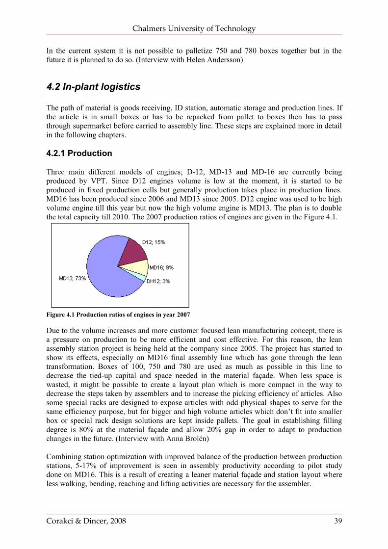
Chalmers University of Technology
In the current system it is not possible to palletize 750 and 780 boxes together but in the future it is planned to do so. (Interview with Helen Andersson)
4.2 In-plant logistics
The path of material is goods receiving, ID station, automatic storage and production lines. If the article is in small boxes or has to be repacked from pallet to boxes then has to pass through supermarket before carried to assembly line. These steps are explained more in detail in the following chapters.
4.2.1 Production
Three main different models of engines; D-12, MD-13 and MD-16 are currently being produced by VPT. Since D12 engines volume is low at the moment, it is started to be produced in fixed production cells but generally production takes place in production lines. MD16 has been produced since 2006 and MD13 since 2005. D12 engine was used to be high volume engine till this year but now the high volume engine is MD13. The plan is to double the total capacity till 2010. The 2007 production ratios of engines are given in the Figure 4.1.
Figure 4.1 Production ratios of engines in year 2007
Due to the volume increases and more customer focused lean manufacturing concept, there is a pressure on production to be more efficient and cost effective. For this reason, the lean assembly station project is being held at the company since 2005. The project has started to show its effects, especially on MD16 final assembly line which has gone through the lean transformation. Boxes of 100, 750 and 780 are used as much as possible in this line to decrease the tied-up capital and space needed in the material façade. When less space is wasted, it might be possible to create a layout plan which is more compact in the way to decrease the steps taken by assemblers and to increase the picking efficiency of articles. Also some special racks are designed to expose articles with odd physical shapes to serve for the same efficiency purpose, but for bigger and high volume articles which don’t fit into smaller box or special rack design solutions are kept inside pallets. The goal in establishing filling degree is 80% at the material façade and allow 20% gap in order to adapt to production changes in the future. (Interview with Anna Brolén)
Combining station optimization with improved balance of the production between production stations, 5-17% of improvement is seen in assembly productivity according to pilot study done on MD16. This is a result of creating a leaner material façade and station layout where less walking, bending, reaching and lifting activities are necessary for the assembler.
Corakci & Dincer, 2008 39
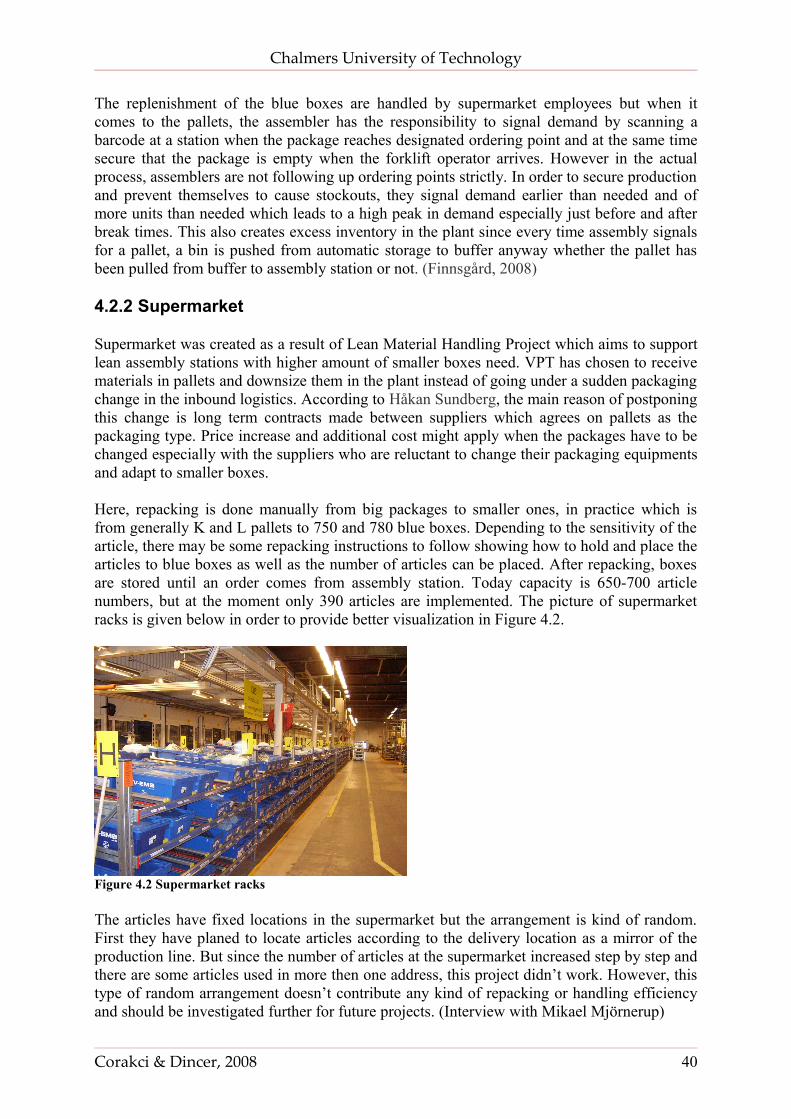
Chalmers University of Technology
The replenishment of the blue boxes are handled by supermarket employees but when it comes to the pallets, the assembler has the responsibility to signal demand by scanning a barcode at a station when the package reaches designated ordering point and at the same time secure that the package is empty when the forklift operator arrives. However in the actual process, assemblers are not following up ordering points strictly. In order to secure production and prevent themselves to cause stockouts, they signal demand earlier than needed and of more units than needed which leads to a high peak in demand especially just before and after break times. This also creates excess inventory in the plant since every time assembly signals for a pallet, a bin is pushed from automatic storage to buffer anyway whether the pallet has been pulled from buffer to assembly station or not. (Finnsgård, 2008)
4.2.2 Supermarket
Supermarket was created as a result of Lean Material Handling Project which aims to support lean assembly stations with higher amount of smaller boxes need. VPT has chosen to receive materials in pallets and downsize them in the plant instead of going under a sudden packaging change in the inbound logistics. According to Håkan Sundberg, the main reason of postponing this change is long term contracts made between suppliers which agrees on pallets as the packaging type. Price increase and additional cost might apply when the packages have to be changed especially with the suppliers who are reluctant to change their packaging equipments and adapt to smaller boxes.
Here, repacking is done manually from big packages to smaller ones, in practice which is from generally K and L pallets to 750 and 780 blue boxes. Depending to the sensitivity of the article, there may be some repacking instructions to follow showing how to hold and place the articles to blue boxes as well as the number of articles can be placed. After repacking, boxes are stored until an order comes from assembly station. Today capacity is 650-700 article numbers, but at the moment only 390 articles are implemented. The picture of supermarket racks is given below in order to provide better visualization in Figure 4.2.
Figure 4.2 Supermarket racks
The articles have fixed locations in the supermarket but the arrangement is kind of random. First they have planed to locate articles according to the delivery location as a mirror of the production line. But since the number of articles at the supermarket increased step by step and there are some articles used in more then one address, this project didn’t work. However, this type of random arrangement doesn’t contribute any kind of repacking or handling efficiency and should be investigated further for future projects. (Interview with Mikael Mjörnerup)
Corakci & Dincer, 2008 40
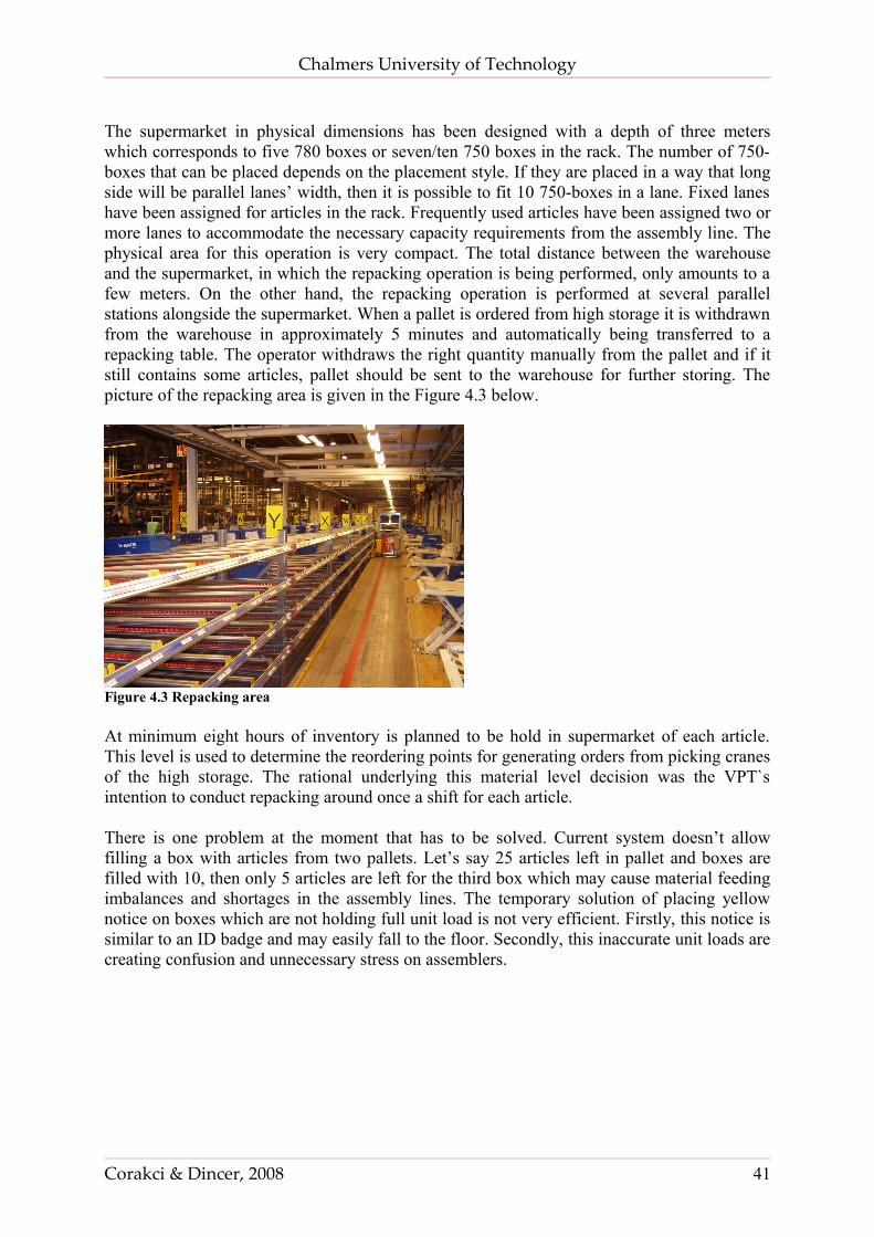
Chalmers University of Technology
The supermarket in physical dimensions has been designed with a depth of three meters which corresponds to five 780 boxes or seven/ten 750 boxes in the rack. The number of 750-boxes that can be placed depends on the placement style. If they are placed in a way that long side will be parallel lanes’ width, then it is possible to fit 10 750-boxes in a lane. Fixed lanes have been assigned for articles in the rack. Frequently used articles have been assigned two or more lanes to accommodate the necessary capacity requirements from the assembly line. The physical area for this operation is very compact. The total distance between the warehouse and the supermarket, in which the repacking operation is being performed, only amounts to a few meters. On the other hand, the repacking operation is performed at several parallel stations alongside the supermarket. When a pallet is ordered from high storage it is withdrawn from the warehouse in approximately 5 minutes and automatically being transferred to a repacking table. The operator withdraws the right quantity manually from the pallet and if it still contains some articles, pallet should be sent to the warehouse for further storing. The picture of the repacking area is given in the Figure 4.3 below.
Figure 4.3 Repacking area
At minimum eight hours of inventory is planned to be hold in supermarket of each article. This level is used to determine the reordering points for generating orders from picking cranes of the high storage. The rational underlying this material level decision was the VPT`s intention to conduct repacking around once a shift for each article.
There is one problem at the moment that has to be solved. Current system doesn’t allow filling a box with articles from two pallets. Let’s say 25 articles left in pallet and boxes are filled with 10, then only 5 articles are left for the third box which may cause material feeding imbalances and shortages in the assembly lines. The temporary solution of placing yellow notice on boxes which are not holding full unit load is not very efficient. Firstly, this notice is similar to an ID badge and may easily fall to the floor. Secondly, this inaccurate unit loads are creating confusion and unnecessary stress on assemblers.
Corakci & Dincer, 2008 41
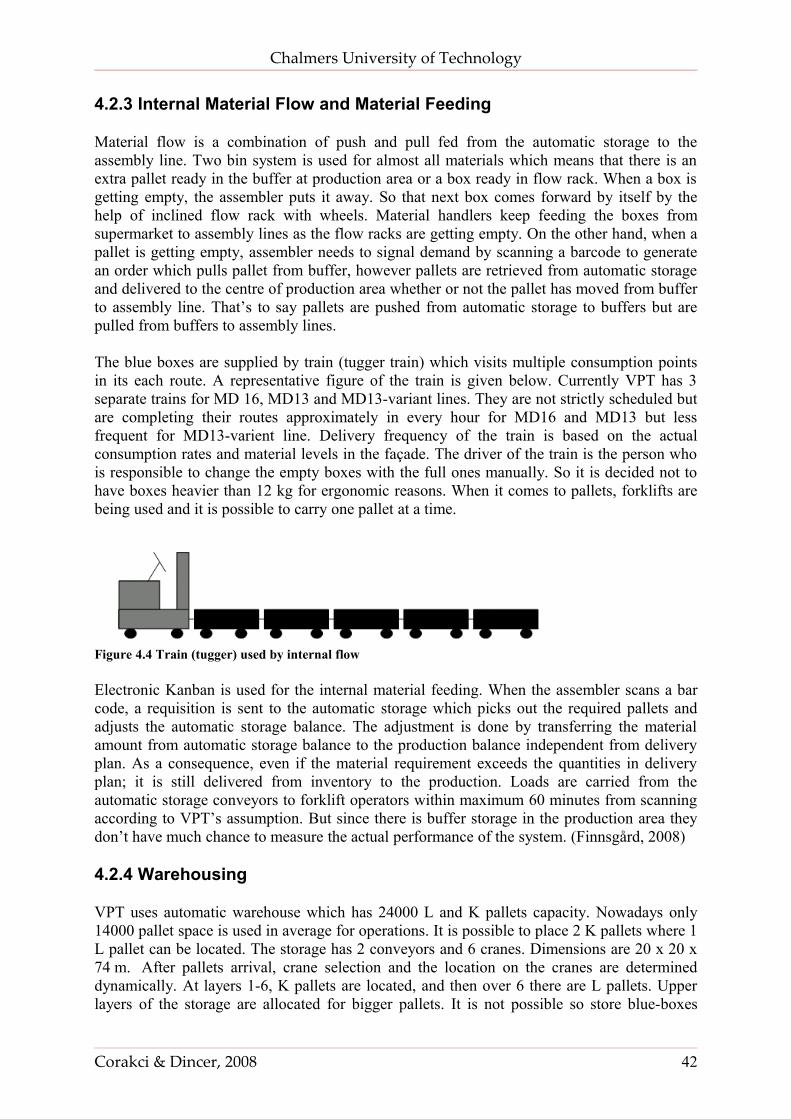
Chalmers University of Technology
4.2.3 Internal Material Flow and Material Feeding
Material flow is a combination of push and pull fed from the automatic storage to the assembly line. Two bin system is used for almost all materials which means that there is an extra pallet ready in the buffer at production area or a box ready in flow rack. When a box is getting empty, the assembler puts it away. So that next box comes forward by itself by the help of inclined flow rack with wheels. Material handlers keep feeding the boxes from supermarket to assembly lines as the flow racks are getting empty. On the other hand, when a pallet is getting empty, assembler needs to signal demand by scanning a barcode to generate an order which pulls pallet from buffer, however pallets are retrieved from automatic storage and delivered to the centre of production area whether or not the pallet has moved from buffer to assembly line. That’s to say pallets are pushed from automatic storage to buffers but are pulled from buffers to assembly lines.
The blue boxes are supplied by train (tugger train) which visits multiple consumption points in its each route. A representative figure of the train is given below. Currently VPT has 3 separate trains for MD 16, MD13 and MD13-variant lines. They are not strictly scheduled but are completing their routes approximately in every hour for MD16 and MD13 but less frequent for MD13-varient line. Delivery frequency of the train is based on the actual consumption rates and material levels in the façade. The driver of the train is the person who is responsible to change the empty boxes with the full ones manually. So it is decided not to have boxes heavier than 12 kg for ergonomic reasons. When it comes to pallets, forklifts are being used and it is possible to carry one pallet at a time.
Figure 4.4 Train (tugger) used by internal flow
Electronic Kanban is used for the internal material feeding. When the assembler scans a bar code, a requisition is sent to the automatic storage which picks out the required pallets and adjusts the automatic storage balance. The adjustment is done by transferring the material amount from automatic storage balance to the production balance independent from delivery plan. As a consequence, even if the material requirement exceeds the quantities in delivery plan; it is still delivered from inventory to the production. Loads are carried from the automatic storage conveyors to forklift operators within maximum 60 minutes from scanning according to VPT’s assumption. But since there is buffer storage in the production area they don’t have much chance to measure the actual performance of the system. (Finnsgård, 2008)
4.2.4 Warehousing
VPT uses automatic warehouse which has 24000 L and K pallets capacity. Nowadays only 14000 pallet space is used in average for operations. It is possible to place 2 K pallets where 1 L pallet can be located. The storage has 2 conveyors and 6 cranes. Dimensions are 20 x 20 x 74 m. After pallets arrival, crane selection and the location on the cranes are determined dynamically. At layers 1-6, K pallets are located, and then over 6 there are L pallets. Upper layers of the storage are allocated for bigger pallets. It is not possible so store blue-boxes
Corakci & Dincer, 2008 42
Chalmers University of Technology
directly; instead, they should have been covered with a pallet base and a lid. The “regular pallets” and “pallets with boxes” are randomly located inside the storage not in particular zones.
Every time pallets are put in or out of the automatic inventories the activity is registered in the inventory system. This makes it difficult to make mistakes that affect the stock balance accuracy according to their investigations. The biggest problem they have at the moment is system breakdowns which disable handling pallets. Conveyor that goes up to the roof is also vulnerable to risks because during breakdowns, pallets can not be reached automatically. These breakdowns may take from 5 minutes to hours. But even in these extreme situations they still can go in and drive the cranes manually.
The pallets are stored until an order is received from assembly station. Retrieving time span depends on the queue on the cranes, queue on conveyor belt, and availability of space at conveyor offloading area. The goal is to deliver one pallet from storage to assembly station less than 1 hour. If there is no queue on the cranes and on the conveyors, delivering a pallet from storage to the assembly station may take place in only 15 minutes. Retrieving times varying from 15 to 60 minutes makes the system highly dependent on the buffer storage in the plant. Without the buffer storage it would be very difficult for production to be able to decide when to signal for replenishment. (Interview with Krister Nordqvist)
They have 2 cranes allocated for the supermarket. The area is called “picking location” or “picking warehouse”. It takes 2-3 minutes from high storage down to the picking location and 5 minutes to deliver articles from picking location to the supermarket. After the repacking if the pallet is not empty yet it goes back to the picking location. When the amounts in pallets are under reordering point then pallets are pulled from high storage to picking location.
4.2.5 ID station
Pallets are moved from goods receiving by auto carriers to a control station that is also known as ID station. Here weight and dimensions of each pallet is controlled and an identity is given which will be used in the high storage. The pallets with mixed loads can also be identified here. Later, automatic conveyors transport pallets from ID station to the automatic warehouse.
4.2.6 Goods receiving
Materials are accepted to the factory through goods receiving points. Truck drivers have to announce arrival and leave delivery notes at the gate at VPT before they drive to the factory area. This is indicated in the material control system to make material controllers know when the material is expected to be available in the factory. Goods receiving open at 6 AM and closes at 9 PM in the evening, but it is still possible to make exceptions and receive goods during all 24 hours as long as warehouse workers are informed in advance. The schedule for the shipments is prepared by VLC. In average 2000-2500 pallets arrive every day. Unloading time is more or less fixed, so unloading 2 trucks with 100 or 1 truck with 200 pallets takes the same amount of time approximately. (Interview with Mimmi Oskarsson)
4.3 Material Controlling
Material controlling function has been divided into two main dimensions:
Corakci & Dincer, 2008 43
Chalmers University of Technology
4.3.1 Internal Material Control
Internal material controllers are responsible for material availability in the production. They make sure that production will receive material on time and if there is a problem they inform both production and external material controllers about its consequences. They control materials through monitoring production and warehouse balance, carry out stocktaking and reorganize materials in the plant when there is a risk of stock outs. When items are small like screws, it is hard to keep track of material in the production so the warehouse balance is used for control.
According to internal material controller Tobias Ljunggren, smaller packages provide better track of inventory as they generally contain materials for a shorter period of time than large packages do. When packages hold material for long period of time, it is difficult to predict requirements and how large quantities that are in production. Production balance value gets less reliable as time passes and the chance of misuse of the articles increases.
4.3.2 External Material Control
External material controllers are responsible for material flow from suppliers to factory gate. They make sure that factory receive materials on time according to the delivery plan and contact suppliers when there is an unexpected situation. There are 13 external material controllers in VPT, 8 of them control the flow directly for assembly area, another 2 work with new part numbers and design change and rest work on material of machinery area. Among those 8 persons who are responsible for the material flow to assembly area, each one has its own group of suppliers and similar articles. For example, one external material controller is responsible for 100 suppliers and 50 to 60 of them are from Sweden. (Interview with Mimmi Oskarsson)
VMR is used by VPT for the communication with suppliers. The ownership belongs to company but still a negotiation based decision is made with suppliers on safety time, transportation lead time and maximum time of replenishment. Safety time shows the time remaining before VPT’s stock levels fall to safety level and maximum time shows the length of time the article is allowed to stay in the inventory. Suppliers should make sure that the replenishment takes place in between these limits. Safety times and maximum times are determined according to the value of the article. For example, when material is valuable, maximum time is set generally shorter to reduce the costs related to inventory holding. (Interview with Mimmi Oskarsson)
Daily updated material requirement, stock balance and received good information are all transferred from MRP system to Pipechain so that; suppliers can monitor delivery suggestions, stock levels and transportation information. Pipechain is an information system used to manage material control and communication between companies by providing exchange of data. At the moment only the most important suppliers have implemented Pipechain but in means of volume of articles, 80% of the total volume is covered by Pipechain. (Interview with Mimmi Oskarsson)
Pipechain allows suppliers to see the total balance including warehouse and production stock balance to synchronize their production according to VPT’s needs. The small and low cost materials such as nuts and bolts are not considered in production stock balance but are included in warehouse stock balance since they are easy to get lost or to be misused in the
Corakci & Dincer, 2008 44
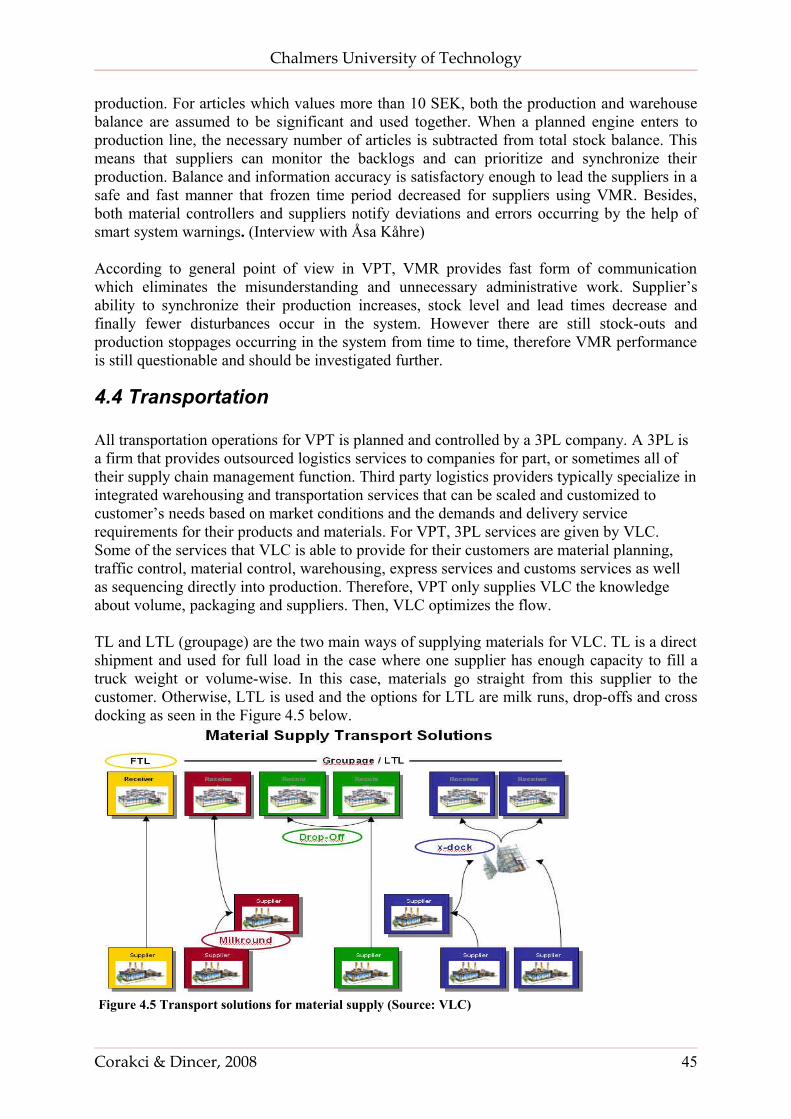
Chalmers University of Technology
production. For articles which values more than 10 SEK, both the production and warehouse balance are assumed to be significant and used together. When a planned engine enters to production line, the necessary number of articles is subtracted from total stock balance. This means that suppliers can monitor the backlogs and can prioritize and synchronize their production. Balance and information accuracy is satisfactory enough to lead the suppliers in a safe and fast manner that frozen time period decreased for suppliers using VMR. Besides, both material controllers and suppliers notify deviations and errors occurring by the help of smart system warnings. (Interview with Åsa Kåhre)
According to general point of view in VPT, VMR provides fast form of communication which eliminates the misunderstanding and unnecessary administrative work. Supplier’s ability to synchronize their production increases, stock level and lead times decrease and finally fewer disturbances occur in the system. However there are still stock-outs and production stoppages occurring in the system from time to time, therefore VMR performance is still questionable and should be investigated further.
4.4 Transportation
All transportation operations for VPT is planned and controlled by a 3PL company. A 3PL is a firm that provides outsourced logistics services to companies for part, or sometimes all of their supply chain management function. Third party logistics providers typically specialize in integrated warehousing and transportation services that can be scaled and customized to customer’s needs based on market conditions and the demands and delivery service requirements for their products and materials. For VPT, 3PL services are given by VLC. Some of the services that VLC is able to provide for their customers are material planning, traffic control, material control, warehousing, express services and customs services as well as sequencing directly into production. Therefore, VPT only supplies VLC the knowledge about volume, packaging and suppliers. Then, VLC optimizes the flow. TL and LTL (groupage) are the two main ways of supplying materials for VLC. TL is a direct shipment and used for full load in the case where one supplier has enough capacity to fill a truck weight or volume-wise. In this case, materials go straight from this supplier to the customer. Otherwise, LTL is used and the options for LTL are milk runs, drop-offs and cross docking as seen in the Figure 4.5 below.
Figure 4.5 Transport solutions for material supply (Source: VLC)
Corakci & Dincer, 2008 45
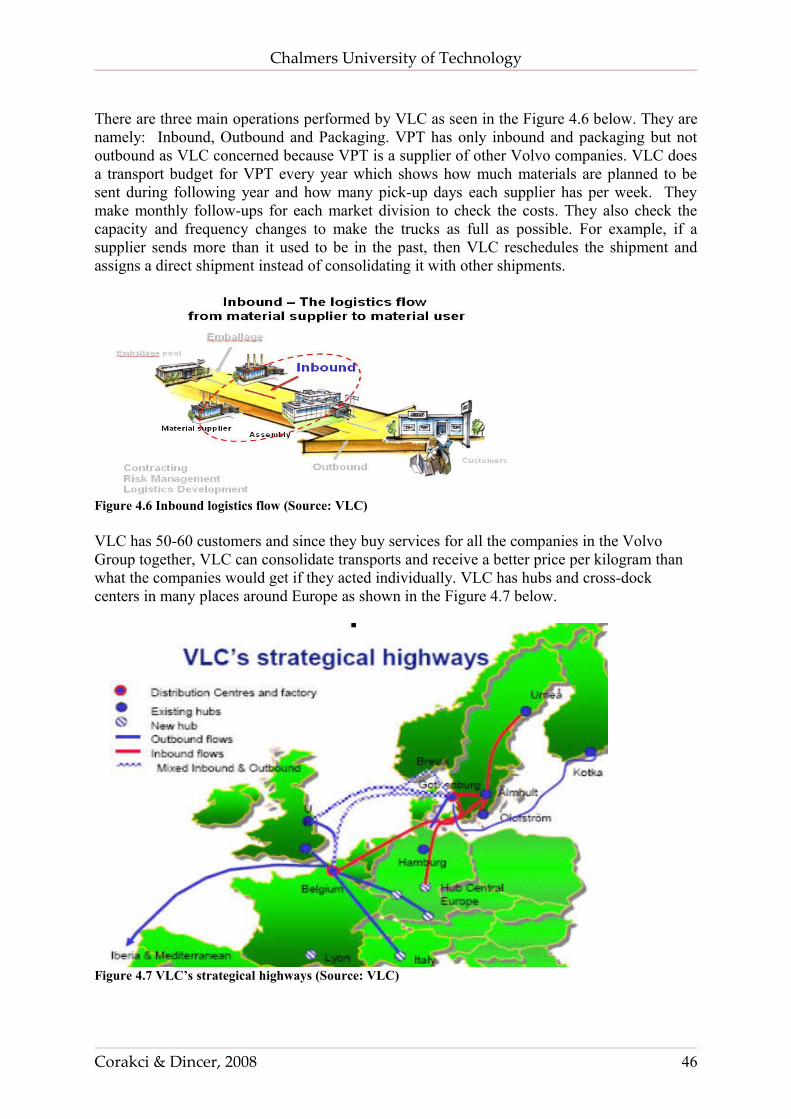
Chalmers University of Technology
There are three main operations performed by VLC as seen in the Figure 4.6 below. They are namely: Inbound, Outbound and Packaging. VPT has only inbound and packaging but not outbound as VLC concerned because VPT is a supplier of other Volvo companies. VLC does a transport budget for VPT every year which shows how much materials are planned to be sent during following year and how many pick-up days each supplier has per week. They make monthly follow-ups for each market division to check the costs. They also check the capacity and frequency changes to make the trucks as full as possible. For example, if a supplier sends more than it used to be in the past, then VLC reschedules the shipment and assigns a direct shipment instead of consolidating it with other shipments.
Figure 4.6 Inbound logistics flow (Source: VLC)
VLC has 50-60 customers and since they buy services for all the companies in the Volvo Group together, VLC can consolidate transports and receive a better price per kilogram than what the companies would get if they acted individually. VLC has hubs and cross-dock centers in many places around Europe as shown in the Figure 4.7 below.
Figure 4.7 VLC’s strategical highways (Source: VLC)
Corakci & Dincer, 2008 46
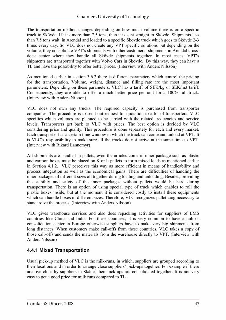
Chalmers University of Technology
The transportation method changes depending on how much volume there is on a specific truck to Skövde. If it is more than 7,5 tons, then it is sent straight to Skövde. Shipments less than 7,5 tons wait in Arendal and loaded to a specific Skövde truck which goes to Skövde 2-3 times every day. So VLC does not create any VPT specific solutions but depending on the volume, they consolidate VPT’s shipments with other customers’ shipments in Arendal cross-dock center where they handle all Skövde shipments together. In most cases, VPT’s shipments are transported together with Volvo Cars in Skövde. By this way, they can have a TL and have the possibility to offer better prices. (Interview with Anders Nilsson)
As mentioned earlier in section 3.6.2 there is different parameters which control the pricing for the transportation. Volume, weight, distance and filling rate are the most important parameters. Depending on these parameters, VLC has a tariff of SEK/kg or SEK/m3 tariff. Consequently, they are able to offer a much better price per unit for a 100% full truck. (Interview with Anders Nilsson)
VLC does not own any trucks. The required capacity is purchased from transporter companies. The procedure is to send out request for quotation to a lot of transporters. VLC specifies which volumes are planned to be carried with the related frequencies and service levels. Transporters get back to VLC with prices. The best option is decided by VLC considering price and quality. This procedure is done separately for each and every market. Each transporter has a certain time window in which the truck can come and unload at VPT. It is VLC’s responsibility to make sure all the trucks do not arrive at the same time to VPT. (Interview with Rikard Lannemyr)
All shipments are handled in pallets, even the articles come in inner package such as plastic and cartoon boxes must be placed on K or L pallets to form mixed loads as mentioned earlier in Section 4.1.2. VLC perceives this way as more efficient in means of handleability and process integration as well as the economical gains. There are difficulties of handling the inner packages of different sizes all together during loading and unloading. Besides, providing the stability and safety of the inner packages without pallets would be hard during transportation. There is an option of using special type of truck which enables to roll the plastic boxes inside, but at the moment it is considered costly to install these equipments which can handle boxes of different sizes. Therefore, VLC recognizes palletizing necessary to standardize the process. (Interview with Anders Nilsson)
VLC gives warehouse services and also does repacking activities for suppliers of EMS countries like China and India. For these countries, it is very common to have a hub or consolidation center in Europe otherwise suppliers have to make very big shipments from long distances. When customers make call-offs from these countries, VLC takes a copy of those call-offs and sends the materials from the warehouse directly to VPT. (Interview with Anders Nilsson)
4.4.1 Mixed Transportation
Usual pick-up method of VLC is the milk-runs, in which, suppliers are grouped according to their locations and in order to arrange close suppliers’ pick-ups together. For example if there are five close-by suppliers in Skåne, their pick-ups are consolidated together. It is not very easy to get a good price for milk runs compared to TL.
Corakci & Dincer, 2008 47
Chalmers University of Technology
The number of suppliers involved in a milk run can differ. Some of the customers are after market companies which require a lot of small shipments since they have special spare parts which are delivered in low frequency and volume. The number of these small suppliers is sometimes up to 1,000. In this case, VLC tries to optimize the schedule as much as possible to fill up the truck. (Interview with Rikard Lannemyr)There are traffic manuals for pick ups from each market. These manuals show the fixed pick-up days from each supplier. For example: Germany is divided into two parts as South and North Germany and there is a certain pickup day for most of them. There are changes in the volume and weight every week, therefore one week one truck might be needed whereas the following week two or three might be necessary. The goods at the supplier should be ready to be picked up anytime within a predetermined time interval for example between 10 and 16. (Interview with Rikard Lannemyr)
In VMI applications, the supplier is the responsible for the transportation to the warehouse. Anders Nilsson recognizes it as a problem for VPT’s supplier network since they have low volumes. Finally, transportation costs will be certainly higher since each supplier will act individually.
4.4.2 Transportation Agreements and Ownership
VPT has FCA agreement with its suppliers which means that VPT takes the full responsibility and the cost of the transportation between companies. The ownership of the materials and related risks are transferred to VPT as soon as goods are loaded to the transporters.
There are fixed shipment dates and time windows for each supplier (or transporter used for that supplier) decided by VLC. When all these fixed windows come together, finally it looks like the example in Table 4.5 from VPT’s point of view.
Table 4.5 An example of time windows for Olssons Transport
Corakci & Dincer, 2008 48
Chalmers University of Technology
5. ALTERNATIVE SYSTEM DESIGN
This chapter explains the assumptions, methodology and logic behind the alternative system design of smaller packages, mixed-load and inbound logistics. This decisions regarding to alternative system design are made after the theory and present situation at VPT are investigated.
5.1 Smaller Package
Since production received significant improvements by the help of Lean Assembly Project so far, it is necessary to investigate if there are further opportunities of using smaller packages. This will increase the production capacity in two ways; first by improving the productivity of existing stations and second by providing extra space for building new stations.
Volvo’s standard packages will be used to create a design called “alternative system” where Volvo’s smaller packages are used as much as possible. The efficiency measures are volume efficiency, total yearly volume, total yearly weight, and total yearly packaging cost as explained in theoretical framework.
It is significant to remind that this design aims to show the effect of solutions where materials are delivered in smaller packages that can be palletized in mixed loads directly from suppliers. It is a result of an approach which sees “repacking” as a waste in the system.
Articles in the plant are examined according to a checklist which included criteria below:
Size: Each article has to be small enough to fit one of the standard inner packages. Lid of the package should be closed when the article is completely inside. This is a constraint for both in-plant and inbound flow set by VPT.
Weight of Article: Each article has to be under a weight limit to be carried in a standard inner package.
Weight of Inner Package: Each full standard inner package should have a weight limit.
Sensitiveness: Each article inside an inner package should be protected properly.
Volvo’s standard boxes; 100, 750 and 780 were used as the smallest package candidates in order to provide a compatible solution to the current system. The stations were visited one by one and all the articles which were kept in packages bigger than 100-cartoon boxes were checked. The ones with 100-cartoon box were assumed as having already the ideal size of possible packaging. Although the main aim was identifying the articles in pallets that are suitable to fit into smaller boxes, articles in 750 and 780 blue boxes were also checked to see if they are efficiently filled. Even the boxes that have been repacked at supermarket were checked because they have been filled for optimization of the in-plant flow. So, boxes are not always full or the lid of the boxes is not always possible to close.
Corakci & Dincer, 2008 49
Chalmers University of Technology
Although pallets are able to hold more parts and require lower transportation, packaging and handling cost per article; smallest packages are preferred to support Lean Assembly Line project as long as they provide good internal filling degree.
5.1.1 Data Collection Process
1. Here is the step by step instruction of the data collection process followed:
2. Hold the article and try to fit it to any of the packages (750, 780 or 100-boxes)
3. If it is not possible to fit it in any of the boxes, note down the article number and pass to the next article in the façade.
4. Count the number of articles after you fill the smallest package as much as possible considering that you can close the package with the lid perfectly.
5. If the article has an irregular shape, also try the larger box. Note down the name of the boxes and the quantities they can hold.
6. If the article seems fragile and already uses some kind of protection in the form of compartments, then assume that these protections should be added to the new packaging also and make the counting accordingly.
7. Fill the data to the excel sheet.
8. If the weight of the alternative package exceeds the limit of 12 kg that Volvo had set for ergonomic reasons, decrease the number of articles that is possible until it reaches down to the limits.
9. If data shows more than one ideal package solution, choose the smaller package as long as it has a high internal filling degree.
5.1.2 Result of the Data Collection
Secondary data collection showed that the 5 heaviest articles which are currently delivered to factory inside 750-boxes are 1.01, 1.12, 1.4, 1.8 and 2.4 kg. The heaviest articles coming inside 780-boxes are 1.44, 1.49, 1.53, 1.65 and 2.92 kg. Our data collections showed approximately the same results. So, we assumed that the articles which are heavier than 1.8 kg are not suitable for 750, 780-plastic or 100-cartoon boxes. Given that assumption, scope of the data collection with respect to whole purchased articles is given in the Table 5.1 below.
The articles which are clarified about their eligibility to fit in small boxes constitute 91% of cumulated total yearly weight and 89% of total yearly volume value but only 65% of the total count of the articles. The main reason behind this is the low accessibility of C-Volume articles in the plant. The meaning of “Total Yearly Weight” and “Total Yearly Volume Value” are explained in the equations below:
Total yearly weight of an article = Weight of a single article * Annual Need
Total yearly volume value of an article = Price of a single article * Annual Need
Corakci & Dincer, 2008 50
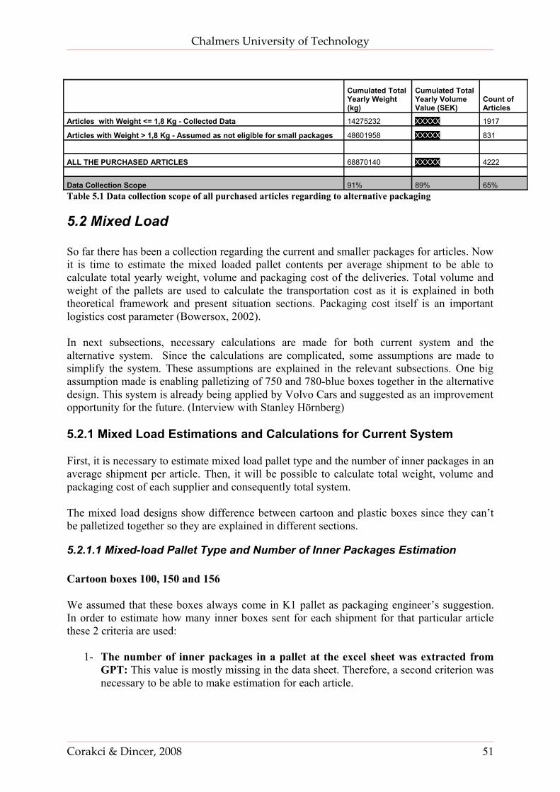
Chalmers University of Technology
Cumulated Total Yearly Weight (kg)
Cumulated Total Yearly Volume Value (SEK)
Count of Articles
Articles with Weight <= 1,8 Kg - Collected Data 14275232 XXXXX 1917
Articles with Weight > 1,8 Kg - Assumed as not eligible for small packages 48601958 XXXXX 831
ALL THE PURCHASED ARTICLES 68870140 XXXXX 4222
Data Collection Scope 91% 89% 65%Table 5.1 Data collection scope of all purchased articles regarding to alternative packaging
5.2 Mixed Load
So far there has been a collection regarding the current and smaller packages for articles. Now it is time to estimate the mixed loaded pallet contents per average shipment to be able to calculate total yearly weight, volume and packaging cost of the deliveries. Total volume and weight of the pallets are used to calculate the transportation cost as it is explained in both theoretical framework and present situation sections. Packaging cost itself is an important logistics cost parameter (Bowersox, 2002).
In next subsections, necessary calculations are made for both current system and the alternative system. Since the calculations are complicated, some assumptions are made to simplify the system. These assumptions are explained in the relevant subsections. One big assumption made is enabling palletizing of 750 and 780-blue boxes together in the alternative design. This system is already being applied by Volvo Cars and suggested as an improvement opportunity for the future. (Interview with Stanley Hörnberg)
5.2.1 Mixed Load Estimations and Calculations for Current System
First, it is necessary to estimate mixed load pallet type and the number of inner packages in an average shipment per article. Then, it will be possible to calculate total weight, volume and packaging cost of each supplier and consequently total system.
The mixed load designs show difference between cartoon and plastic boxes since they can’t be palletized together so they are explained in different sections.
5.2.1.1 Mixed-load Pallet Type and Number of Inner Packages Estimation
Cartoon boxes 100, 150 and 156
We assumed that these boxes always come in K1 pallet as packaging engineer’s suggestion. In order to estimate how many inner boxes sent for each shipment for that particular article these 2 criteria are used:
1- The number of inner packages in a pallet at the excel sheet was extracted from GPT: This value is mostly missing in the data sheet. Therefore, a second criterion was necessary to be able to make estimation for each article.
Corakci & Dincer, 2008 51
Chalmers University of Technology
2- Total number of respective packages sent by the supplier in a shipment: This is not only the quantity of packages for that particular article. The other articles sent from same supplier in the same package type also considered to apply mixed loads. Then this value divided into supplier turnover to get the number of respective packages sent in a shipment.
The maximum value of these two numbers is accepted as the number of packages sent in a shipment. If this number of articles is exceeding K1 pallets capacity, limit number accepted as the number of packages in K1 pallet. The limit is to fit 30 100-cartoon, 20 156-cartoon or 8 150-cartoon boxes in a single K1 pallet.
Example:
For article X;1- There are 25 inner packages in a pallet (outer package) according to excel sheet extracted from GPT. 2- 220 100-cartoon boxes are sent by the supplier in a year and the supplier turnover is 10. Then the quantity of 100-cartoon boxes sent in a shipment is estimated as 220/10 = 22. So the maximum of these two numbers, 25, is assumed as the number of packages sent in a shipment inside a single K1 pallet.
Plastic Boxes 750 and 780
They can be sent in K1, K2, K3, L1, L2, L3 or L4 pallets. First two criteria given above for the cartoon-boxes are used to decide the maximum number of boxes sent in a shipment. After that this value is matched with the capacity of each pallet type and the one which provides a higher filling rate is chosen.
Example:If there are 22 750-boxes sent in a shipment then this boxes can fit into only L3 and L4, but L3 is chosen as a pallet since it will provide a better filling rate.
5.2.1.2 Volume estimations
Volume of one single inner package and total yearly volume for a particular article are estimated by the equations below:
Volume of a inner package (m3) = Volume of the outer package (m3) / Average number of inner packages per outer package
Total yearly volume of the article (m3) = Number of inner packages necessary in a year * Volume of a inner package (m3)
And;
Number of inner packages necessary in a year = Annual need / Number of articles hold by an inner package
Corakci & Dincer, 2008 52
Chalmers University of Technology
5.2.1.3 Weight estimation
Weight of one single inner package and total yearly weight for a particular article are estimated by the equations below:
Cartoon boxes 100, 150 and 156
When carrying cartoon boxes; a single K pallet base, frame, spacer and lid are necessary for K1. All these weights should be added up and divided into number of inner packages in the outer package-K1 to find the average weight of a single cartoon box for that particular article.
Average weight of one cartoon box carried in K1 = Weight of K pallet base + Weight of K pallet frame + Weight of K pallet spacer + Weight of K pallet lid + Quantity of cartoon boxes carried in a Pallet *
(Weight of a cartoon-box itself + Weight of articles in a cartoon box) / Quantity of cartoon boxes carried in a pallet
Total yearly weight of the article (kg) = Number of inner packages necessary in a year * Weight of a inner package (kg)
Plastic boxes 750 and 780
When carrying 750 and 780-boxes; pallet base and plastic lid is necessary for the K1, K2, K3, L1, L2, L3, L4 outer packages. There is no need for spacers and frames.
Average weight of one plastic box carried in L or K pallet = Weight of pallet base used + Weight of pallet lid + Quantity of plastic boxes carried in a Pallet * (Weight of a plastic box itself + Weight of articles in a
plastic box ) / Quantity of blue boxes carried in a pallet
5.2.1.4 Packaging transaction fee cost
Packaging transaction fee is the amount paid to Volvo Logistics for reusable plastic boxes and pallets for each transaction. There is no rental fee for 100-cartoon box since they are not reusable. The cartoon boxes have the ownership cost for each usage.
Cartoon boxes 100, 150 and 156
When carrying cartoon boxes; a single K pallet base, frame, spacer and lid are necessary for K1. All these packaging fees should be added up and divided into number of inner packages in the outer package-K1 to find the average packaging cost of a single cartoon box for that particular article.
Average packaging cost of one cartoon box carried in K1 = Packaging cost of K pallet base + Packaging cost of K pallet frame + Packaging cost of K pallet spacer + Packaging cost of K pallet lid + Quantity of
cartoon boxes carried in a Pallet * (Packaging cost of a cartoon-box itself + Packaging cost of articles in a cartoon box) / Quantity of cartoon boxes carried in a pallet
Corakci & Dincer, 2008 53
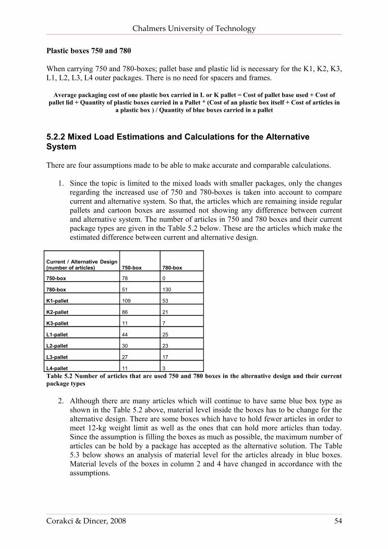
Chalmers University of Technology
Plastic boxes 750 and 780
When carrying 750 and 780-boxes; pallet base and plastic lid is necessary for the K1, K2, K3, L1, L2, L3, L4 outer packages. There is no need for spacers and frames.
Average packaging cost of one plastic box carried in L or K pallet = Cost of pallet base used + Cost of pallet lid + Quantity of plastic boxes carried in a Pallet * (Cost of an plastic box itself + Cost of articles in
a plastic box ) / Quantity of blue boxes carried in a pallet
5.2.2 Mixed Load Estimations and Calculations for the Alternative System
There are four assumptions made to be able to make accurate and comparable calculations.
1. Since the topic is limited to the mixed loads with smaller packages, only the changes regarding the increased use of 750 and 780-boxes is taken into account to compare current and alternative system. So that, the articles which are remaining inside regular pallets and cartoon boxes are assumed not showing any difference between current and alternative system. The number of articles in 750 and 780 boxes and their current package types are given in the Table 5.2 below. These are the articles which make the estimated difference between current and alternative design.
Current / Alternative Design (number of articles) 750-box 780-box
750-box 78 0
780-box 51 130
K1-pallet 109 53
K2-pallet 86 21
K3-pallet 11 7
L1-pallet 44 25
L2-pallet 30 23
L3-pallet 27 17
L4-pallet 11 3Table 5.2 Number of articles that are used 750 and 780 boxes in the alternative design and their current package types
2. Although there are many articles which will continue to have same blue box type as shown in the Table 5.2 above, material level inside the boxes has to be change for the alternative design. There are some boxes which have to hold fewer articles in order to meet 12-kg weight limit as well as the ones that can hold more articles than today. Since the assumption is filling the boxes as much as possible, the maximum number of articles can be hold by a package has accepted as the alternative solution. The Table 5.3 below shows an analysis of material level for the articles already in blue boxes. Material levels of the boxes in column 2 and 4 have changed in accordance with the assumptions.
Corakci & Dincer, 2008 54
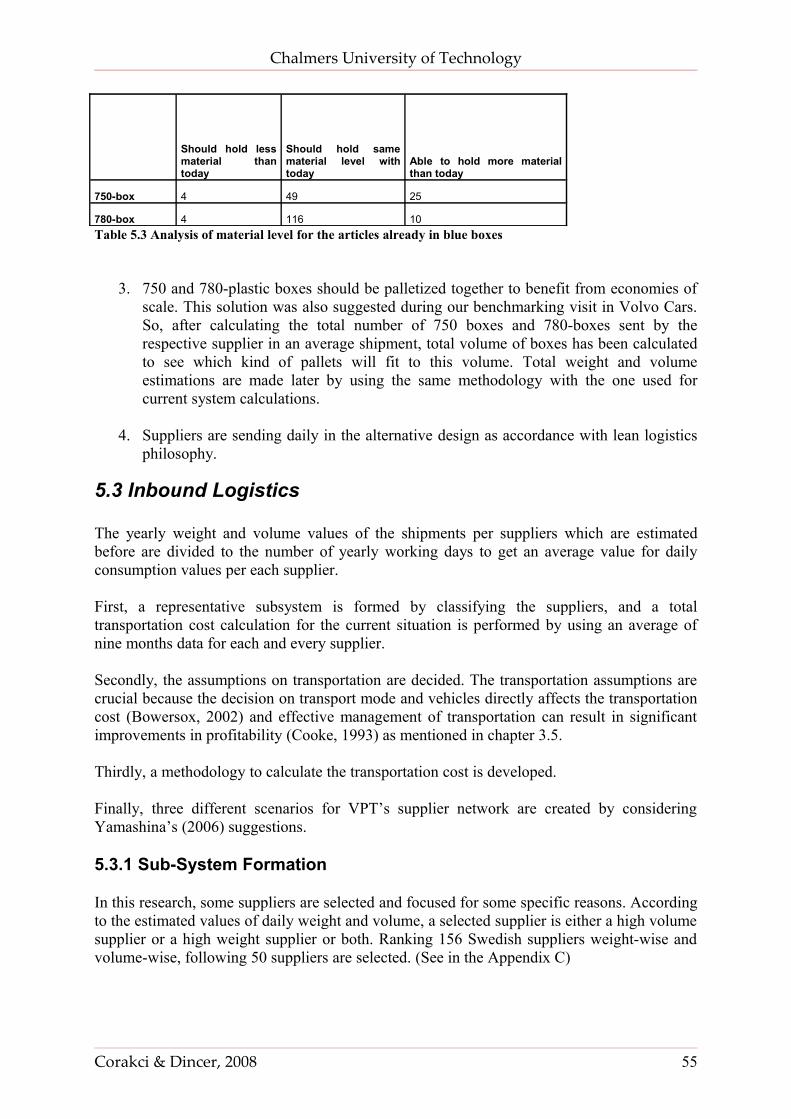
Chalmers University of Technology
Should hold less material than today
Should hold same material level with today
Able to hold more material than today
750-box 4 49 25
780-box 4 116 10Table 5.3 Analysis of material level for the articles already in blue boxes
3. 750 and 780-plastic boxes should be palletized together to benefit from economies of scale. This solution was also suggested during our benchmarking visit in Volvo Cars. So, after calculating the total number of 750 boxes and 780-boxes sent by the respective supplier in an average shipment, total volume of boxes has been calculated to see which kind of pallets will fit to this volume. Total weight and volume estimations are made later by using the same methodology with the one used for current system calculations.
4. Suppliers are sending daily in the alternative design as accordance with lean logistics philosophy.
5.3 Inbound Logistics
The yearly weight and volume values of the shipments per suppliers which are estimated before are divided to the number of yearly working days to get an average value for daily consumption values per each supplier.
First, a representative subsystem is formed by classifying the suppliers, and a total transportation cost calculation for the current situation is performed by using an average of nine months data for each and every supplier.
Secondly, the assumptions on transportation are decided. The transportation assumptions are crucial because the decision on transport mode and vehicles directly affects the transportation cost (Bowersox, 2002) and effective management of transportation can result in significant improvements in profitability (Cooke, 1993) as mentioned in chapter 3.5.
Thirdly, a methodology to calculate the transportation cost is developed.
Finally, three different scenarios for VPT’s supplier network are created by considering Yamashina’s (2006) suggestions.
5.3.1 Sub-System Formation
In this research, some suppliers are selected and focused for some specific reasons. According to the estimated values of daily weight and volume, a selected supplier is either a high volume supplier or a high weight supplier or both. Ranking 156 Swedish suppliers weight-wise and volume-wise, following 50 suppliers are selected. (See in the Appendix C)
Corakci & Dincer, 2008 55
Chalmers University of Technology
Thus, a sub-system of 50 suppliers is created. Although this sub-system represents 32% of total number of the suppliers in Sweden, it represents 90% of the total picture both weight and volume-wise. A summary of the sub-system can be seen in the Table 5.4 below:Total weight (KG) Sub-system Weight (KG) 140227,7 126320,3 0,90 Total Volume (M3) Sub-system Volume (M3) 504,7 456,0 0,90 # Total Suppliers # Sub-system Suppliers 156 50 0,32
Table 5.4 Summary of sub-system
5.3.1.1 Current Cost Calculation Methodology In order to calculate the current cost of the sub-system, such a method was used:
1. By using a nine months of cost data from January 2007 to September 2007, an average cost for all suppliers in the sub-system was calculated as the example seen in the Table 5.5.
Cost Supplier 16 Supplier 17 Supplier 18 Supplier 19 Supplier 20P1 2851 4081 1681 34300 29196P2 3719 2505 1563 32544 21820P3 3543 1925 2315 38180 25217P4 2654 421 1550 30789 21995P5 6656 2886 2075 34012 27333P6 7425 1185 1337 26848 25144P7 1856 284 616 15649 7551P8 4880 2235 955 25637 20359P9 4914 945 1657 32472 20117AVG 4277,5 1829,6 1527,6 30047,8 22081,3
Table 5.5 Average cost for all suppliers in the sub-system
2. By adding all costs for 50 suppliers together, sub-system’s current cost is calculated. Since cost data for 4 of the suppliers in the system were missing, the actual calculation was done for 46 of the suppliers and the average current cost of the sub-system was calculated as 436605 SEK monthly.
5.3.2 Assumptions for Transportation Mode
In this research, road transportation and five main types of vehicles are used:
1- Full Truck: It has a capacity of 36 tons in weight and 126 cubic meters in volume. This type of trucks is allowed to use only in domestic traffic in Sweden since they exceed the greatest length allowed in most European countries. It is a combination of a regular truck and a semi-trailer. (Lumsden, 2002) It looks like as in the picture below:
Corakci & Dincer, 2008 56
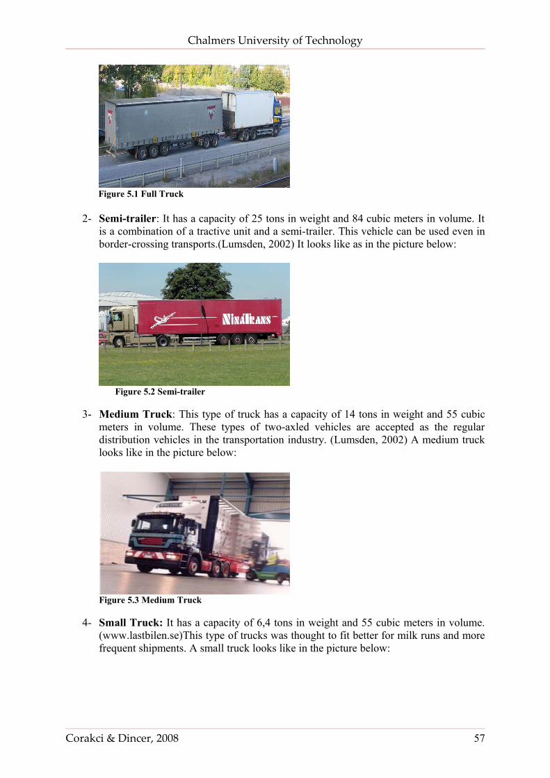
Chalmers University of Technology
Figure 5.1 Full Truck
2- Semi-trailer: It has a capacity of 25 tons in weight and 84 cubic meters in volume. It is a combination of a tractive unit and a semi-trailer. This vehicle can be used even in border-crossing transports.(Lumsden, 2002) It looks like as in the picture below:
Figure 5.2 Semi-trailer
3- Medium Truck: This type of truck has a capacity of 14 tons in weight and 55 cubic meters in volume. These types of two-axled vehicles are accepted as the regular distribution vehicles in the transportation industry. (Lumsden, 2002) A medium truck looks like in the picture below:
Figure 5.3 Medium Truck
4- Small Truck: It has a capacity of 6,4 tons in weight and 55 cubic meters in volume. (www.lastbilen.se)This type of trucks was thought to fit better for milk runs and more frequent shipments. A small truck looks like in the picture below:
Corakci & Dincer, 2008 57
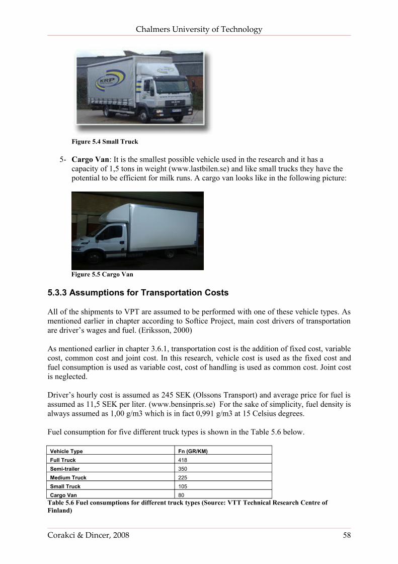
Chalmers University of Technology
Figure 5.4 Small Truck
5- Cargo Van: It is the smallest possible vehicle used in the research and it has a capacity of 1,5 tons in weight (www.lastbilen.se) and like small trucks they have the potential to be efficient for milk runs. A cargo van looks like in the following picture:
Figure 5.5 Cargo Van
5.3.3 Assumptions for Transportation Costs
All of the shipments to VPT are assumed to be performed with one of these vehicle types. As mentioned earlier in chapter according to Softice Project, main cost drivers of transportation are driver’s wages and fuel. (Eriksson, 2000)
As mentioned earlier in chapter 3.6.1, transportation cost is the addition of fixed cost, variable cost, common cost and joint cost. In this research, vehicle cost is used as the fixed cost and fuel consumption is used as variable cost, cost of handling is used as common cost. Joint cost is neglected.
Driver’s hourly cost is assumed as 245 SEK (Olssons Transport) and average price for fuel is assumed as 11,5 SEK per liter. (www.bensinpris.se) For the sake of simplicity, fuel density is always assumed as 1,00 g/m3 which is in fact 0,991 g/m3 at 15 Celsius degrees.
Fuel consumption for five different truck types is shown in the Table 5.6 below.
Vehicle Type Fn (GR/KM)Full Truck 418Semi-trailer 350Medium Truck 225Small Truck 105Cargo Van 80
Table 5.6 Fuel consumptions for different truck types (Source: VTT Technical Research Centre of Finland)
Corakci & Dincer, 2008 58
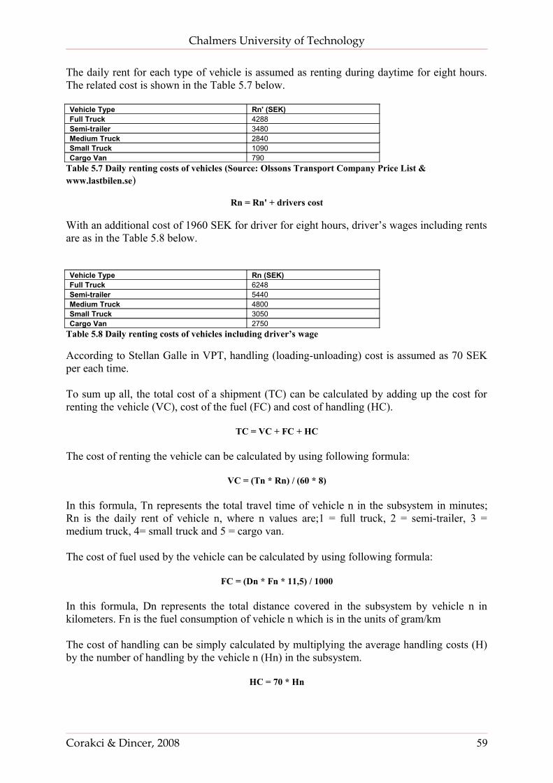
Chalmers University of Technology
The daily rent for each type of vehicle is assumed as renting during daytime for eight hours. The related cost is shown in the Table 5.7 below.
Vehicle Type Rn' (SEK)Full Truck 4288Semi-trailer 3480Medium Truck 2840Small Truck 1090Cargo Van 790
Table 5.7 Daily renting costs of vehicles (Source: Olssons Transport Company Price List & www.lastbilen.se)
Rn = Rn' + drivers cost
With an additional cost of 1960 SEK for driver for eight hours, driver’s wages including rents are as in the Table 5.8 below.
Vehicle Type Rn (SEK)Full Truck 6248Semi-trailer 5440Medium Truck 4800Small Truck 3050Cargo Van 2750
Table 5.8 Daily renting costs of vehicles including driver’s wage
According to Stellan Galle in VPT, handling (loading-unloading) cost is assumed as 70 SEK per each time.
To sum up all, the total cost of a shipment (TC) can be calculated by adding up the cost for renting the vehicle (VC), cost of the fuel (FC) and cost of handling (HC).
TC = VC + FC + HC
The cost of renting the vehicle can be calculated by using following formula:
VC = (Tn * Rn) / (60 * 8)
In this formula, Tn represents the total travel time of vehicle n in the subsystem in minutes; Rn is the daily rent of vehicle n, where n values are;1 = full truck, 2 = semi-trailer, 3 = medium truck, 4= small truck and 5 = cargo van.
The cost of fuel used by the vehicle can be calculated by using following formula:
FC = (Dn * Fn * 11,5) / 1000
In this formula, Dn represents the total distance covered in the subsystem by vehicle n in kilometers. Fn is the fuel consumption of vehicle n which is in the units of gram/km
The cost of handling can be simply calculated by multiplying the average handling costs (H) by the number of handling by the vehicle n (Hn) in the subsystem.
HC = 70 * Hn
Corakci & Dincer, 2008 59
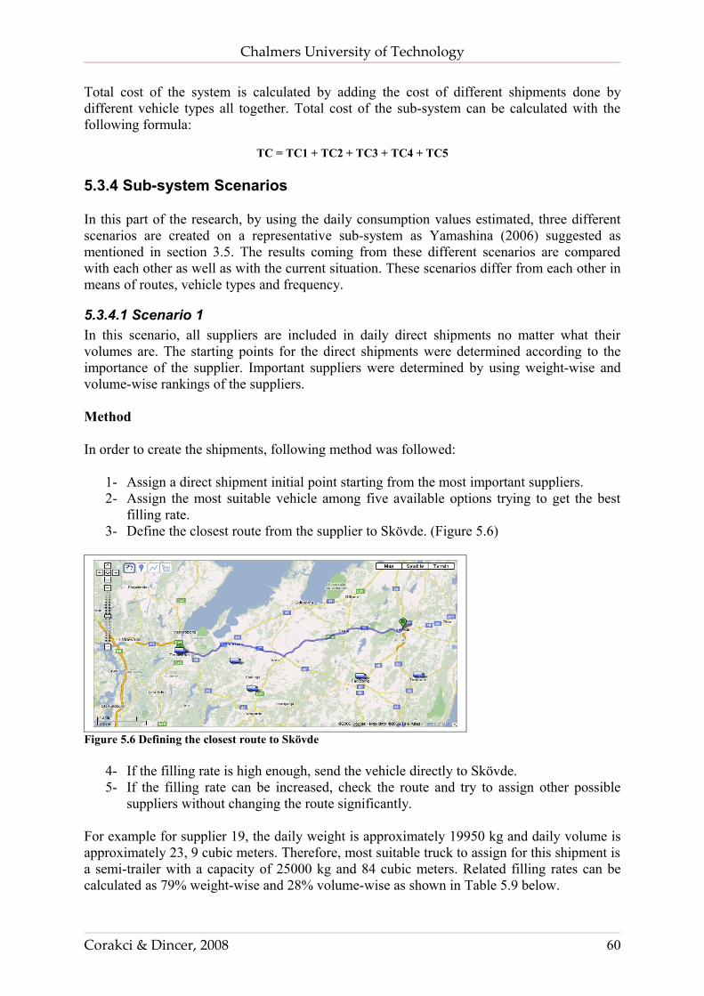
Chalmers University of Technology
Total cost of the system is calculated by adding the cost of different shipments done by different vehicle types all together. Total cost of the sub-system can be calculated with the following formula:
TC = TC1 + TC2 + TC3 + TC4 + TC5
5.3.4 Sub-system Scenarios
In this part of the research, by using the daily consumption values estimated, three different scenarios are created on a representative sub-system as Yamashina (2006) suggested as mentioned in section 3.5. The results coming from these different scenarios are compared with each other as well as with the current situation. These scenarios differ from each other in means of routes, vehicle types and frequency.
5.3.4.1 Scenario 1In this scenario, all suppliers are included in daily direct shipments no matter what their volumes are. The starting points for the direct shipments were determined according to the importance of the supplier. Important suppliers were determined by using weight-wise and volume-wise rankings of the suppliers.
Method
In order to create the shipments, following method was followed:
1- Assign a direct shipment initial point starting from the most important suppliers.2- Assign the most suitable vehicle among five available options trying to get the best
filling rate.3- Define the closest route from the supplier to Skövde. (Figure 5.6)
Figure 5.6 Defining the closest route to Skövde
4- If the filling rate is high enough, send the vehicle directly to Skövde.5- If the filling rate can be increased, check the route and try to assign other possible
suppliers without changing the route significantly.
For example for supplier 19, the daily weight is approximately 19950 kg and daily volume is approximately 23, 9 cubic meters. Therefore, most suitable truck to assign for this shipment is a semi-trailer with a capacity of 25000 kg and 84 cubic meters. Related filling rates can be calculated as 79% weight-wise and 28% volume-wise as shown in Table 5.9 below.
Corakci & Dincer, 2008 60
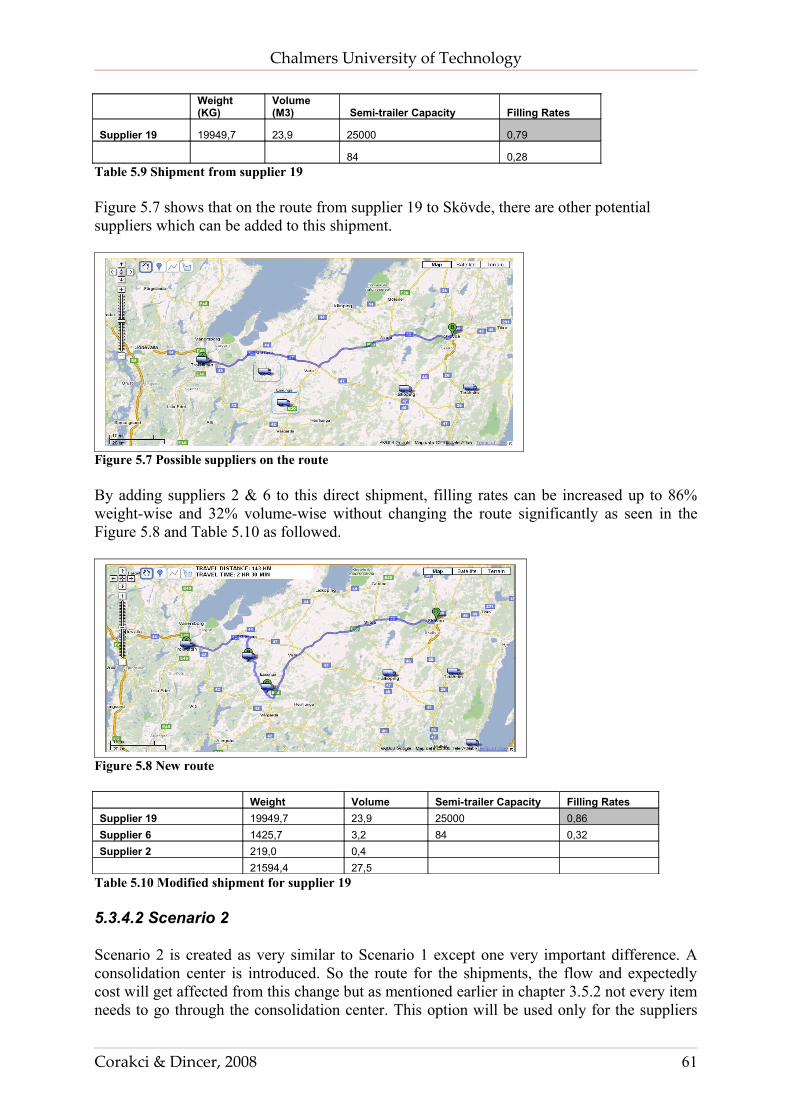
Chalmers University of Technology
Weight (KG)
Volume (M3) Semi-trailer Capacity Filling Rates
Supplier 19 19949,7 23,9 25000 0,79
84 0,28Table 5.9 Shipment from supplier 19 Figure 5.7 shows that on the route from supplier 19 to Skövde, there are other potential suppliers which can be added to this shipment.
Figure 5.7 Possible suppliers on the route
By adding suppliers 2 & 6 to this direct shipment, filling rates can be increased up to 86% weight-wise and 32% volume-wise without changing the route significantly as seen in the Figure 5.8 and Table 5.10 as followed.
Figure 5.8 New route
Weight Volume Semi-trailer Capacity Filling RatesSupplier 19 19949,7 23,9 25000 0,86Supplier 6 1425,7 3,2 84 0,32Supplier 2 219,0 0,4 21594,4 27,5
Table 5.10 Modified shipment for supplier 19
5.3.4.2 Scenario 2
Scenario 2 is created as very similar to Scenario 1 except one very important difference. A consolidation center is introduced. So the route for the shipments, the flow and expectedly cost will get affected from this change but as mentioned earlier in chapter 3.5.2 not every item needs to go through the consolidation center. This option will be used only for the suppliers
Corakci & Dincer, 2008 61
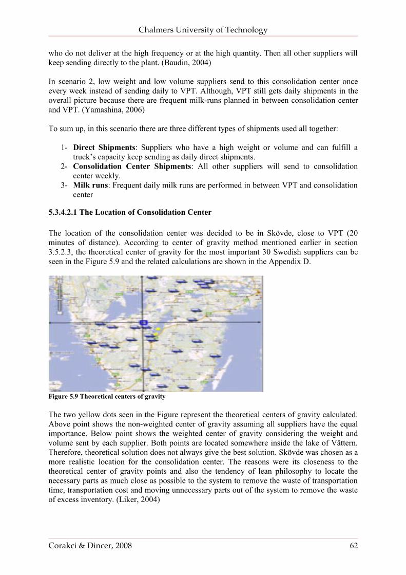
Chalmers University of Technology
who do not deliver at the high frequency or at the high quantity. Then all other suppliers will keep sending directly to the plant. (Baudin, 2004)
In scenario 2, low weight and low volume suppliers send to this consolidation center once every week instead of sending daily to VPT. Although, VPT still gets daily shipments in the overall picture because there are frequent milk-runs planned in between consolidation center and VPT. (Yamashina, 2006)
To sum up, in this scenario there are three different types of shipments used all together:
1- Direct Shipments: Suppliers who have a high weight or volume and can fulfill a truck’s capacity keep sending as daily direct shipments.
2- Consolidation Center Shipments: All other suppliers will send to consolidation center weekly.
3- Milk runs: Frequent daily milk runs are performed in between VPT and consolidation center
5.3.4.2.1 The Location of Consolidation Center
The location of the consolidation center was decided to be in Skövde, close to VPT (20 minutes of distance). According to center of gravity method mentioned earlier in section 3.5.2.3, the theoretical center of gravity for the most important 30 Swedish suppliers can be seen in the Figure 5.9 and the related calculations are shown in the Appendix D.
Figure 5.9 Theoretical centers of gravity
The two yellow dots seen in the Figure represent the theoretical centers of gravity calculated. Above point shows the non-weighted center of gravity assuming all suppliers have the equal importance. Below point shows the weighted center of gravity considering the weight and volume sent by each supplier. Both points are located somewhere inside the lake of Vättern. Therefore, theoretical solution does not always give the best solution. Skövde was chosen as a more realistic location for the consolidation center. The reasons were its closeness to the theoretical center of gravity points and also the tendency of lean philosophy to locate the necessary parts as much close as possible to the system to remove the waste of transportation time, transportation cost and moving unnecessary parts out of the system to remove the waste of excess inventory. (Liker, 2004)
Corakci & Dincer, 2008 62
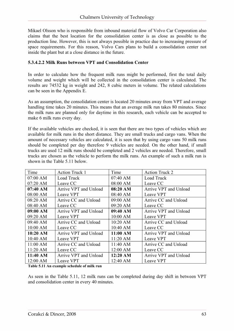
Chalmers University of Technology
Mikael Olsson who is responsible from inbound material flow of Volvo Car Corporation also claims that the best location for the consolidation center is as close as possible to the production line. However, this is not always possible in practice due to increasing pressure of space requirements. For this reason, Volvo Cars plans to build a consolidation center not inside the plant but at a close distance in the future.
5.3.4.2.2 Milk Runs between VPT and Consolidation Center
In order to calculate how the frequent milk runs might be performed, first the total daily volume and weight which will be collected in the consolidation center is calculated. The results are 74532 kg in weight and 242, 8 cubic meters in volume. The related calculations can be seen in the Appendix E.
As an assumption, the consolidation center is located 20 minutes away from VPT and average handling time takes 20 minutes. This means that an average milk run takes 80 minutes. Since the milk runs are planned only for daytime in this research, each vehicle can be accepted to make 6 milk runs every day.
If the available vehicles are checked, it is seen that there are two types of vehicles which are available for milk runs in the short distance. They are small trucks and cargo vans. When the amount of necessary vehicles are calculated, it is seen that by using cargo vans 50 milk runs should be completed per day therefore 9 vehicles are needed. On the other hand, if small trucks are used 12 milk runs should be completed and 2 vehicles are needed. Therefore, small trucks are chosen as the vehicle to perform the milk runs. An example of such a milk run is shown in the Table 5.11 below.
Time Action Truck 1 Time Action Truck 207:00 AM07:20 AM
Load TruckLeave CC
07:40 AM08:00 AM
Load Truck Leave CC
07:40 AM08:00 AM
Arrive VPT and UnloadLeave VPT
08:20 AM08:40 AM
Arrive VPT and UnloadLeave VPT
08:20 AM08:40 AM
Arrive CC and UnloadLeave CC
09:00 AM09:20 AM
Arrive CC and UnloadLeave CC
09:00 AM09:20 AM
Arrive VPT and UnloadLeave VPT
09:40 AM10:00 AM
Arrive VPT and UnloadLeave VPT
09:40 AM10:00 AM
Arrive CC and UnloadLeave CC
10:20 AM10:40 AM
Arrive CC and UnloadLeave CC
10:20 AM10:40 AM
Arrive VPT and UnloadLeave VPT
11:00 AM11:20 AM
Arrive VPT and UnloadLeave VPT
11:00 AM11:20 AM
Arrive CC and UnloadLeave CC
11:40 AM12:00 AM
Arrive CC and UnloadLeave CC
11:40 AM12:00 AM
Arrive VPT and UnloadLeave VPT
12:20 AM12:40 AM
Arrive VPT and UnloadLeave VPT
Table 5.11 An example schedule of milk run
As seen in the Table 5.11, 12 milk runs can be completed during day shift in between VPT and consolidation center in every 40 minutes.
Corakci & Dincer, 2008 63
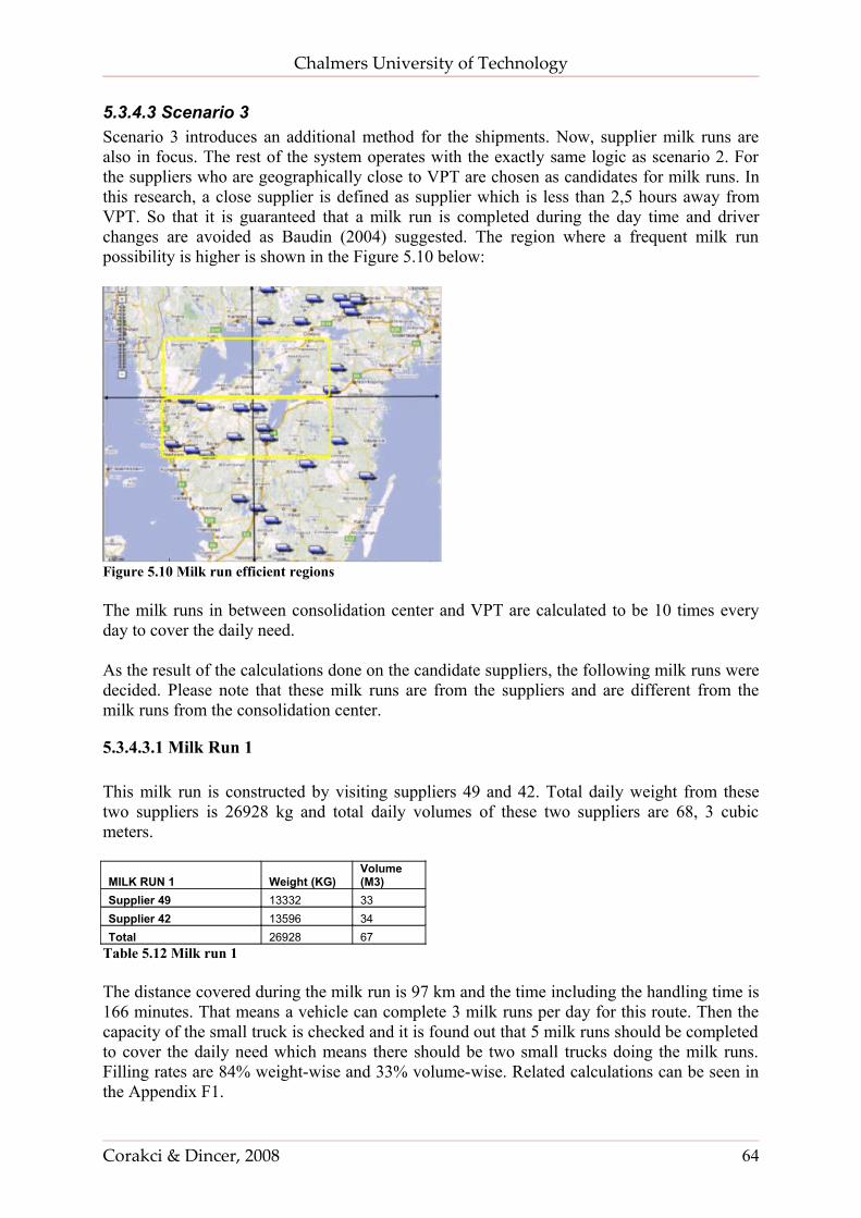
Chalmers University of Technology
5.3.4.3 Scenario 3Scenario 3 introduces an additional method for the shipments. Now, supplier milk runs are also in focus. The rest of the system operates with the exactly same logic as scenario 2. For the suppliers who are geographically close to VPT are chosen as candidates for milk runs. In this research, a close supplier is defined as supplier which is less than 2,5 hours away from VPT. So that it is guaranteed that a milk run is completed during the day time and driver changes are avoided as Baudin (2004) suggested. The region where a frequent milk run possibility is higher is shown in the Figure 5.10 below:
Figure 5.10 Milk run efficient regions
The milk runs in between consolidation center and VPT are calculated to be 10 times every day to cover the daily need.
As the result of the calculations done on the candidate suppliers, the following milk runs were decided. Please note that these milk runs are from the suppliers and are different from the milk runs from the consolidation center.
5.3.4.3.1 Milk Run 1
This milk run is constructed by visiting suppliers 49 and 42. Total daily weight from these two suppliers is 26928 kg and total daily volumes of these two suppliers are 68, 3 cubic meters.
MILK RUN 1 Weight (KG)Volume (M3)
Supplier 49 13332 33Supplier 42 13596 34Total 26928 67
Table 5.12 Milk run 1
The distance covered during the milk run is 97 km and the time including the handling time is 166 minutes. That means a vehicle can complete 3 milk runs per day for this route. Then the capacity of the small truck is checked and it is found out that 5 milk runs should be completed to cover the daily need which means there should be two small trucks doing the milk runs. Filling rates are 84% weight-wise and 33% volume-wise. Related calculations can be seen in the Appendix F1.
Corakci & Dincer, 2008 64
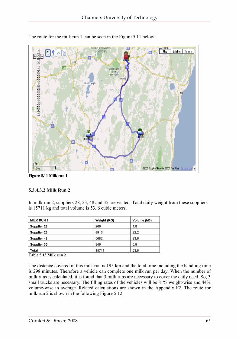
Chalmers University of Technology
The route for the milk run 1 can be seen in the Figure 5.11 below:
Figure 5.11 Milk run 1
5.3.4.3.2 Milk Run 2
In milk run 2, suppliers 28, 23, 48 and 35 are visited. Total daily weight from these suppliers is 15711 kg and total volume is 53, 6 cubic meters.
MILK RUN 2 Weight (KG) Volume (M3)
Supplier 28 266 1,8
Supplier 23 8916 22,2
Supplier 48 5682 23,6
Supplier 35 846 5,9
Total 15711 53,6Table 5.13 Milk run 2
The distance covered in this milk run is 195 km and the total time including the handling time is 298 minutes. Therefore a vehicle can complete one milk run per day. When the number of milk runs is calculated, it is found that 3 milk runs are necessary to cover the daily need. So, 3 small trucks are necessary. The filling rates of the vehicles will be 81% weight-wise and 44% volume-wise in average. Related calculations are shown in the Appendix F2. The route for milk run 2 is shown in the following Figure 5.12:
Corakci & Dincer, 2008 65
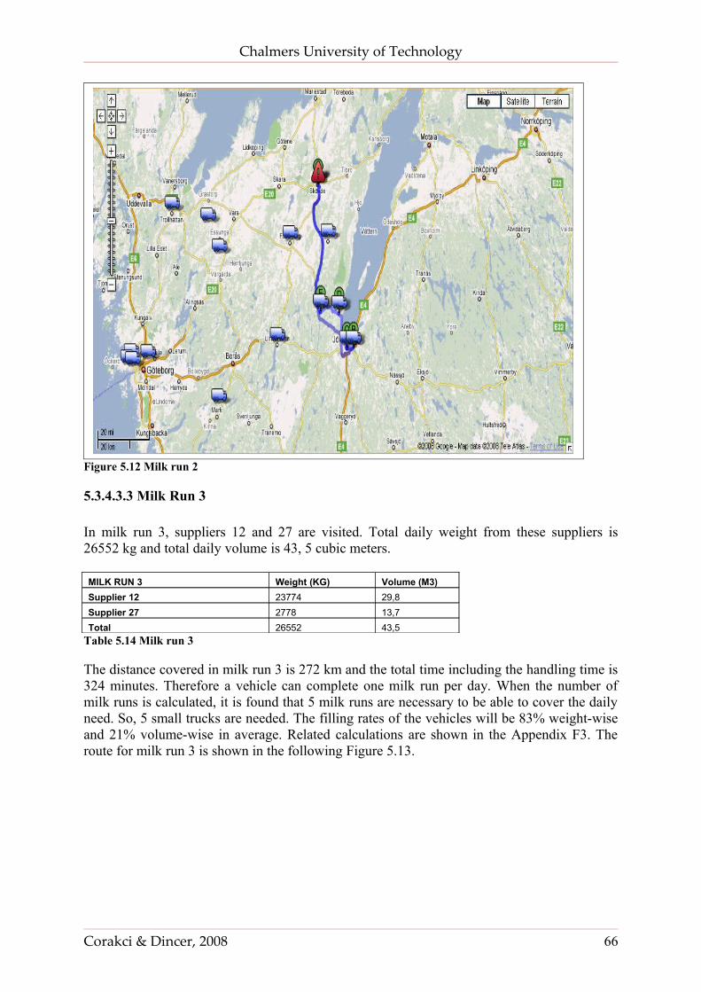
Chalmers University of Technology
Figure 5.12 Milk run 2
5.3.4.3.3 Milk Run 3
In milk run 3, suppliers 12 and 27 are visited. Total daily weight from these suppliers is 26552 kg and total daily volume is 43, 5 cubic meters.
MILK RUN 3 Weight (KG) Volume (M3)Supplier 12 23774 29,8Supplier 27 2778 13,7Total 26552 43,5
Table 5.14 Milk run 3 The distance covered in milk run 3 is 272 km and the total time including the handling time is 324 minutes. Therefore a vehicle can complete one milk run per day. When the number of milk runs is calculated, it is found that 5 milk runs are necessary to be able to cover the daily need. So, 5 small trucks are needed. The filling rates of the vehicles will be 83% weight-wise and 21% volume-wise in average. Related calculations are shown in the Appendix F3. The route for milk run 3 is shown in the following Figure 5.13.
Corakci & Dincer, 2008 66
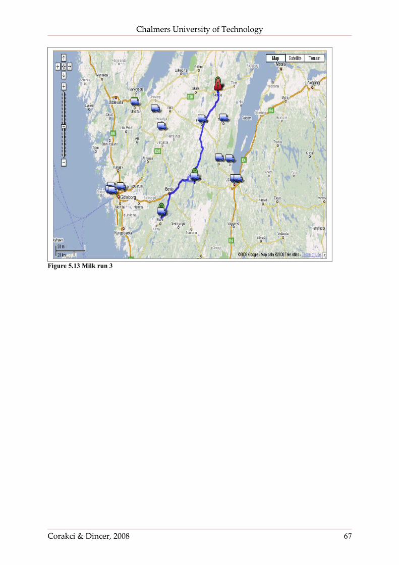
Chalmers University of Technology
Figure 5.13 Milk run 3
Corakci & Dincer, 2008 67
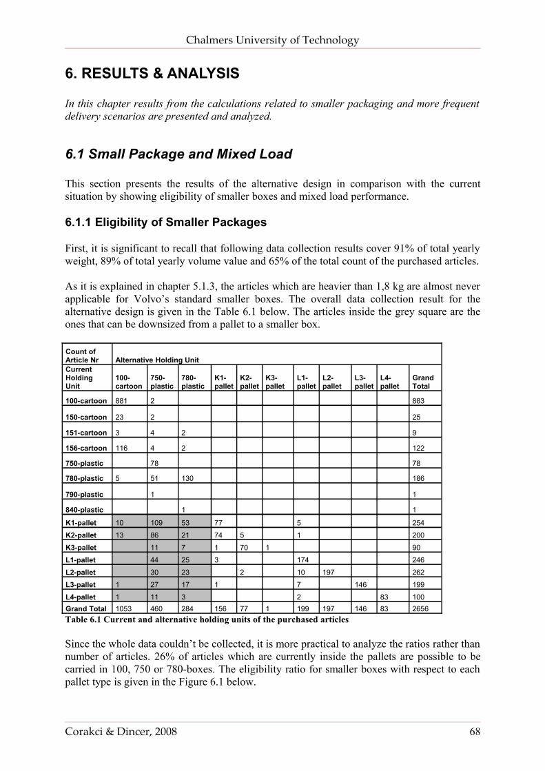
Chalmers University of Technology
6. RESULTS & ANALYSIS
In this chapter results from the calculations related to smaller packaging and more frequent delivery scenarios are presented and analyzed.
6.1 Small Package and Mixed Load
This section presents the results of the alternative design in comparison with the current situation by showing eligibility of smaller boxes and mixed load performance.
6.1.1 Eligibility of Smaller Packages
First, it is significant to recall that following data collection results cover 91% of total yearly weight, 89% of total yearly volume value and 65% of the total count of the purchased articles.
As it is explained in chapter 5.1.3, the articles which are heavier than 1,8 kg are almost never applicable for Volvo’s standard smaller boxes. The overall data collection result for the alternative design is given in the Table 6.1 below. The articles inside the grey square are the ones that can be downsized from a pallet to a smaller box.
Count of Article Nr Alternative Holding UnitCurrent Holding Unit
100-cartoon
750-plastic
780-plastic
K1-pallet
K2-pallet
K3-pallet
L1-pallet
L2-pallet
L3-pallet
L4-pallet
Grand Total
100-cartoon 881 2 883
150-cartoon 23 2 25
151-cartoon 3 4 2 9
156-cartoon 116 4 2 122
750-plastic 78 78
780-plastic 5 51 130 186
790-plastic 1 1
840-plastic 1 1
K1-pallet 10 109 53 77 5 254
K2-pallet 13 86 21 74 5 1 200
K3-pallet 11 7 1 70 1 90
L1-pallet 44 25 3 174 246
L2-pallet 30 23 2 10 197 262
L3-pallet 1 27 17 1 7 146 199
L4-pallet 1 11 3 2 83 100Grand Total 1053 460 284 156 77 1 199 197 146 83 2656Table 6.1 Current and alternative holding units of the purchased articles
Since the whole data couldn’t be collected, it is more practical to analyze the ratios rather than number of articles. 26% of articles which are currently inside the pallets are possible to be carried in 100, 750 or 780-boxes. The eligibility ratio for smaller boxes with respect to each pallet type is given in the Figure 6.1 below.
Corakci & Dincer, 2008 68
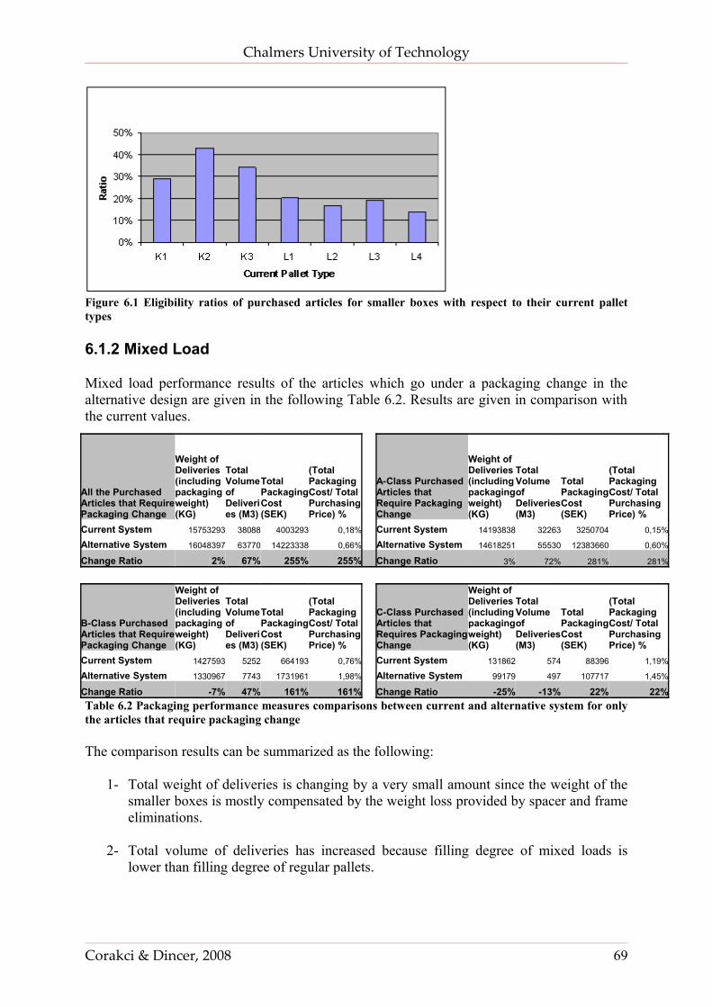
Chalmers University of Technology
Figure 6.1 Eligibility ratios of purchased articles for smaller boxes with respect to their current pallet types
6.1.2 Mixed Load
Mixed load performance results of the articles which go under a packaging change in the alternative design are given in the following Table 6.2. Results are given in comparison with the current values.
All the Purchased Articles that Require Packaging Change
Weight of Deliveries (including packaging weight) (KG)
Total Volume of Deliveries (M3)
Total Packaging Cost (SEK)
(Total Packaging Cost/ Total Purchasing Price) %
A-Class Purchased Articles that Require Packaging Change
Weight of Deliveries (including packaging weight) (KG)
Total Volume of Deliveries (M3)
Total Packaging Cost (SEK)
(Total Packaging Cost/ Total Purchasing Price) %
Current System 15753293 38088 4003293 0,18% Current System 14193838 32263 3250704 0,15%
Alternative System 16048397 63770 14223338 0,66% Alternative System 14618251 55530 12383660 0,60%
Change Ratio 2% 67% 255% 255% Change Ratio 3% 72% 281% 281%
B-Class Purchased Articles that Require Packaging Change
Weight of Deliveries (including packaging weight) (KG)
Total Volume of Deliveries (M3)
Total Packaging Cost (SEK)
(Total Packaging Cost/ Total Purchasing Price) %
C-Class Purchased Articles that Requires Packaging Change
Weight of Deliveries (including packaging weight) (KG)
Total Volume of Deliveries (M3)
Total Packaging Cost (SEK)
(Total Packaging Cost/ Total Purchasing Price) %
Current System 1427593 5252 664193 0,76% Current System 131862 574 88396 1,19%
Alternative System 1330967 7743 1731961 1,98% Alternative System 99179 497 107717 1,45%
Change Ratio -7% 47% 161% 161% Change Ratio -25% -13% 22% 22%Table 6.2 Packaging performance measures comparisons between current and alternative system for only the articles that require packaging change
The comparison results can be summarized as the following:
1- Total weight of deliveries is changing by a very small amount since the weight of the smaller boxes is mostly compensated by the weight loss provided by spacer and frame eliminations.
2- Total volume of deliveries has increased because filling degree of mixed loads is lower than filling degree of regular pallets.
Corakci & Dincer, 2008 69
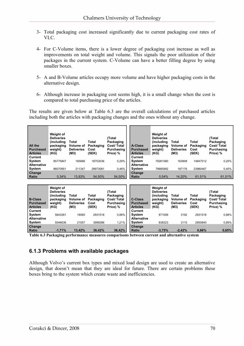
Chalmers University of Technology
3- Total packaging cost increased significantly due to current packaging cost rates of VLC.
4- For C-Volume items, there is a lower degree of packaging cost increase as well as improvements on total weight and volume. This signals the poor utilization of their packages in the current system. C-Volume can have a better filling degree by using smaller boxes.
5- A and B-Volume articles occupy more volume and have higher packaging costs in the alternative design.
6- Although increase in packaging cost seems high, it is a small change when the cost is compared to total purchasing price of the articles.
The results are given below at Table 6.3 are the overall calculations of purchased articles including both the articles with packaging changes and the ones without any change.
All the Purchased Articles
Weight of Deliveries (including packaging weight) (KG)
Total Volume of Deliveries (M3)
Total Packaging Cost (SEK)
(Total Packaging Cost/ Total Purchasing Price) %
A-Class Purchased Articles
Weight of Deliveries (including packaging weight) (KG)
Total Volume of Deliveries (M3)
Total Packaging Cost (SEK)
(Total Packaging Cost/ Total Purchasing Price) %
Current System 85775847 185666 18753036 0,29%
Current System 79261580 163908 14847512 0,25%
Alternative System 86070951 211347 28973081 0,46%
Alternative System 79685992 187176 23980467 0,40%
Change Ratio 0,34% 13,83% 54,50% 54,50%
Change Ratio 0,54% 14,20% 61,51% 61,51%
B-Class Purchased Articles
Weight of Deliveries (including packaging weight) (KG)
Total Volume of Deliveries (M3)
Total Packaging Cost (SEK)
(Total Packaging Cost/ Total Purchasing Price) %
C-Class Purchased Articles
Weight of Deliveries (including packaging weight) (KG)
Total Volume of Deliveries (M3)
Total Packaging Cost (SEK)
(Total Packaging Cost/ Total Purchasing Price) %
Current System 5643261 18565 2931518 0,88%
Current System 871006 3192 2931518 0,88%
Alternative System 5546636 21057 3999286 1,21%
Alternative System 838323 3115 2950840 0,89%
Change Ratio -1,71% 13,42% 36,42% 36,42%
Change Ratio -3,75% -2,42% 0,66% 0,65%
Table 6.3 Packaging performance measures comparisons between current and alternative system
6.1.3 Problems with available packages
Although Volvo’s current box types and mixed load design are used to create an alternative design, that doesn’t mean that they are ideal for future. There are certain problems these boxes bring to the system which create waste and inefficiencies.
Corakci & Dincer, 2008 70
Chalmers University of Technology
6.1.3.1 Problems with cartoon boxes
These boxes can not be palletized together with the blue boxes in mixed load design. So, it creates inefficiencies in the flow in terms of total volume and weight.
Although these boxes are considered cheap by the purchasers, they are not environmental friendly since they are not reusable. Approximately 2000000 SEK is spent to use 645000 cartoon boxes yearly for purchased articles and there is no way to reuse these boxes.
Besides, assemblers need to put an effort to open their seal with a cutter and walk additional steps to throw them to dustbin. These are operations which waste the time of assemblers and detract their attention from the actual value-added work. Liker (2004)
6.1.3.2 Problems with pallets
Since the focus of this study is mainly analyzing the applicability of mixed loads, data has only been collected for small and light articles which can fit into small plastic boxes. Nevertheless, it has been the general observation that, articles used by VPT are not generally big enough to justify the use of as many big pallets as today. Consequently, big pallets hold parts which are enough to cover for days and cause excess inventories in the assembly line and inside the plant.
There is also the issue of cleanliness and reliability that has to be taken into account. Pallets are not cleanable, so the articles are covered with oil and dirt in the long run which lead quality decreases, defects and even break downs in engines. Pallets are not accepted as reliable either; they have the possibility of breakdown and cause slowdowns in the production. (Interview with Petrus Dagman)
Excess inventory, unnecessary movements, waiting times and defects caused by pallets as mentioned above are among seven wastes of lean philosophy. (Liker, 2004)
6.1.3.3 Problems with blue boxes
Firstly, the standard Volvo plastic boxes are conical which decrease the efficient use of space since they occupy as much space as a rectangular block that can hold these boxes inside.
Usable Filling Efficiency of a Box = Inner Volume / Outer Volume
For 750-box;Usable Filling Efficiency is; (0,0157 / 0,027 )*100 = 58%
For 780-box;Usable Filling Efficiency is; (0,0366 / 0,053)*100 = 69%
As shown by the calculations above, packages have low usable filling efficiencies which lead low material façade and tugger train utilization.
Besides, although the actual material holding capacity of the 750 and 780-boxes are 40 kg, the weight limit of 12 kg set by VPT for the internal flow prevents the efficient use of box capacities. 23% of this weight limit is already made up by the tare of 780-box (including its
Corakci & Dincer, 2008 71
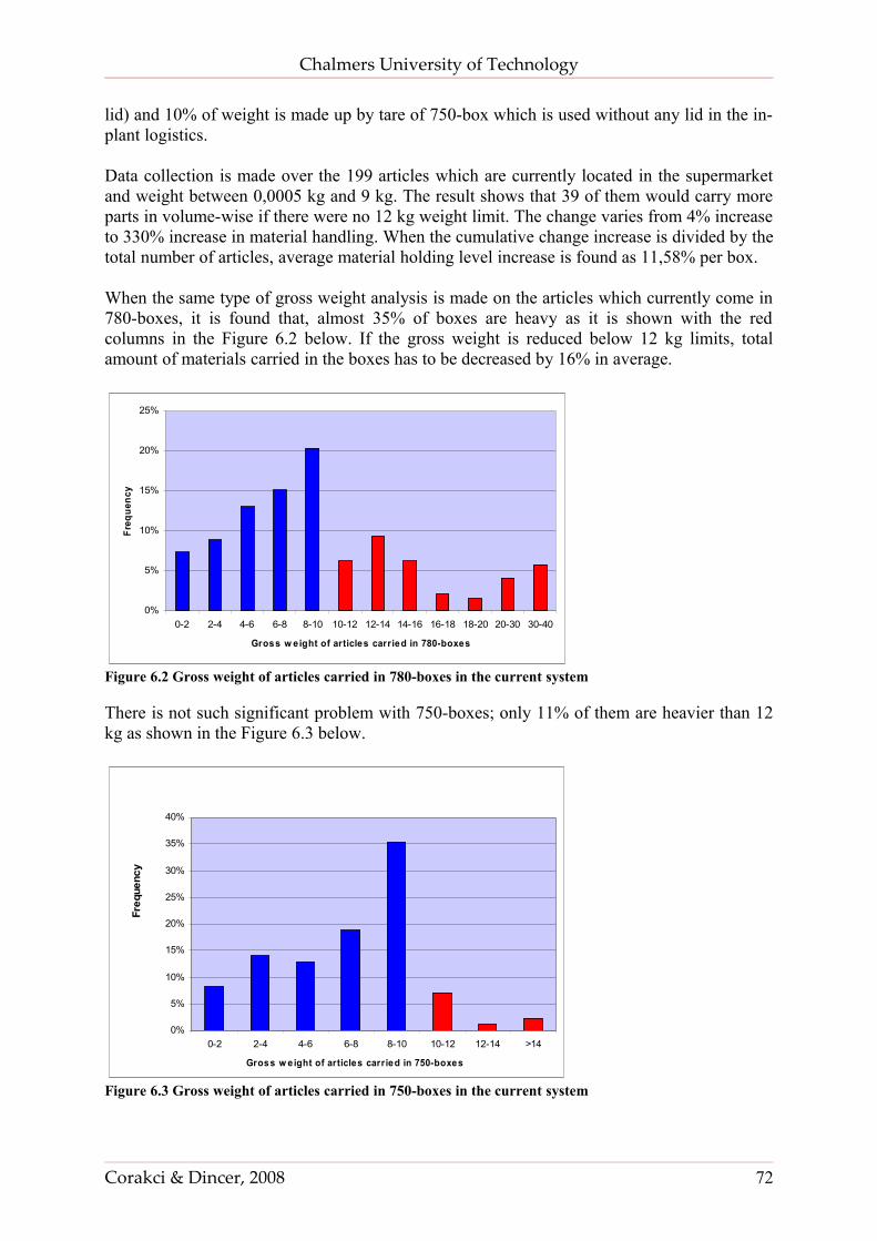
Chalmers University of Technology
lid) and 10% of weight is made up by tare of 750-box which is used without any lid in the in-plant logistics.
Data collection is made over the 199 articles which are currently located in the supermarket and weight between 0,0005 kg and 9 kg. The result shows that 39 of them would carry more parts in volume-wise if there were no 12 kg weight limit. The change varies from 4% increase to 330% increase in material handling. When the cumulative change increase is divided by the total number of articles, average material holding level increase is found as 11,58% per box.
When the same type of gross weight analysis is made on the articles which currently come in 780-boxes, it is found that, almost 35% of boxes are heavy as it is shown with the red columns in the Figure 6.2 below. If the gross weight is reduced below 12 kg limits, total amount of materials carried in the boxes has to be decreased by 16% in average.
0%
5%
10%
15%
20%
25%
0-2 2-4 4-6 6-8 8-10 10-12 12-14 14-16 16-18 18-20 20-30 30-40
Gross w eight of articles carried in 780-boxes
Freq
uenc
y
Figure 6.2 Gross weight of articles carried in 780-boxes in the current system
There is not such significant problem with 750-boxes; only 11% of them are heavier than 12 kg as shown in the Figure 6.3 below.
Freq
uenc
y
0%
5%
10%
15%
20%
25%
30%
35%
40%
0-2 2-4 4-6 6-8 8-10 10-12 12-14 >14
Gross w eight of articles carried in 750-boxes
Figure 6.3 Gross weight of articles carried in 750-boxes in the current system
Corakci & Dincer, 2008 72
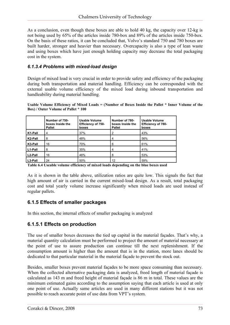
Chalmers University of Technology
As a conclusion, even though these boxes are able to hold 40 kg, the capacity over 12-kg is not being used by 65% of the articles inside 780-box and 89% of the articles inside 750-box. On the basis of these ratios, it can be concluded that, Volvo’s standard 750 and 780 boxes are built harder, stronger and heavier than necessary. Overcapacity is also a type of lean waste and using boxes which have just enough holding capacity may decrease the total packaging cost in the system.
6.1.3.4 Problems with mixed-load design
Design of mixed load is very crucial in order to provide safety and efficiency of the packaging during both transportation and material handling. Efficiency can be corresponded with the external usable volume efficiency of the mixed load during inbound transportation and handleability during material handling.
Usable Volume Efficiency of Mixed Loads = (Number of Boxes Inside the Pallet * Inner Volume of the Box) / Outer Volume of Pallet * 100
Number of 750-boxes Inside the Pallet
Usable Volume Efficiency of 750-boxes
Number of 780-boxes Inside the Pallet
Usable Volume Efficiency of 780-boxes
K1-Pall 4 37% 2 43%
K2-Pall 8 48% 4 56%
K3-Pall 16 70% 6 61%
L1-Pall 8 35% 4 41%
L2-Pall 16 46% 8 53%
L3-Pall 24 50% 12 59%Table 6.4 Useable volume efficiency of mixed loads depending on the blue boxes used
As it is shown in the table above, utilization ratios are quite low. This signals the fact that high amount of air is carried in the current mixed-load design. As a result, total packaging cost and total yearly volume increase significantly when mixed loads are used instead of regular pallets.
6.1.5 Effects of smaller packages
In this section, the internal effects of smaller packaging is analyzed
6.1.5.1 Effects on production
The use of smaller boxes decreases the tied up capital in the material façades. That’s why, a material quantity calculation must be performed to project the amount of material necessary at the point of use to assure production can continue till the next replenishment. If the consumption amount is higher than the amount that is in the station, more lanes should be dedicated to that particular material in the material façade to prevent the stock out.
Besides, smaller boxes prevent material façades to be more space consuming than necessary. When the collected alternative packaging data is analyzed, freed length of material façade is calculated as 143 m and freed height of material façade is 86 m in total. These values are the minimum estimated gains according to the assumption saying that each article is used at only one point of use. Actually same articles are used in many different stations but it was not possible to reach accurate point of use data from VPT’s system.
Corakci & Dincer, 2008 73
Chalmers University of Technology
According to study at station 1500 of MD13 line, 67% of line side space has freed by using smaller boxes. (Finnsgård, 2008)
Freed up space can be used for station layout optimization and line balancing. When the stations are optimized and well balanced the flow is continuous since there is no waiting times between stations. Additionally the changes in layout will decrease the waste in terms, movement of assemblers and waiting times. This will create a smooth flow where productivity levels are increased and response times are improved.
Freed up space also creates the possibility to built new stations when capacity increase is required.
6.1.5.2 Effects on internal transportation
According to calculations made over collected data, the number of 750-boxes used in the system will increase approximately 300% and 780-boxes by 380%. This will require probably higher number of tugger trains and personal.
The problems of internal material shortages will mostly be solved since smaller packages provide better visibility and control of the remaining amount of the articles left in the stations.
Here is the estimated number of boxes transported in the alternative design.
532 articles inside 750-box 1124448 boxes /year, 5041 boxes/day
346 articles inside 780 –box 707046 boxes /year, 3142 boxes/day
This increase in the number of boxes will consequently bring the decrease of pallets and forklift need in the internal transportation. The total number of pallets will decrease by 27% which can be considered as great benefit for decreasing the forklift related costs.
6.1.5.3 Effects on warehousing
When there is increased number of smaller packages used in the assembly, there will be fewer pallets in the system which will make automatic warehouse obsolete in time. Warehousing is an activity that requires inventory holding in the system. The more time necessary for replenishment, the greater the inventory and the greater the inventory cost. When pallets are carried from good receiving directly to the production, no resources will be wasted for storing and retrieving and yet pallets will be delivered to exact point of use without any delay.
6.2 Inbound Logistics Flow Analysis
Inbound logistics flow analysis is done by comparing the scenarios in means of total transportation cost, amount of monthly shipments and the frequency. The focus is on the changes and how these values are affected from the changing parameters for each scenario. Later, problems about consolidation center and mixed transportation are also discussed.
As mentioned in section 5.1, the articles are transported in smaller boxes as much as possible but there are still some heavy and big articles which can not be transported in blue boxes.
Corakci & Dincer, 2008 74
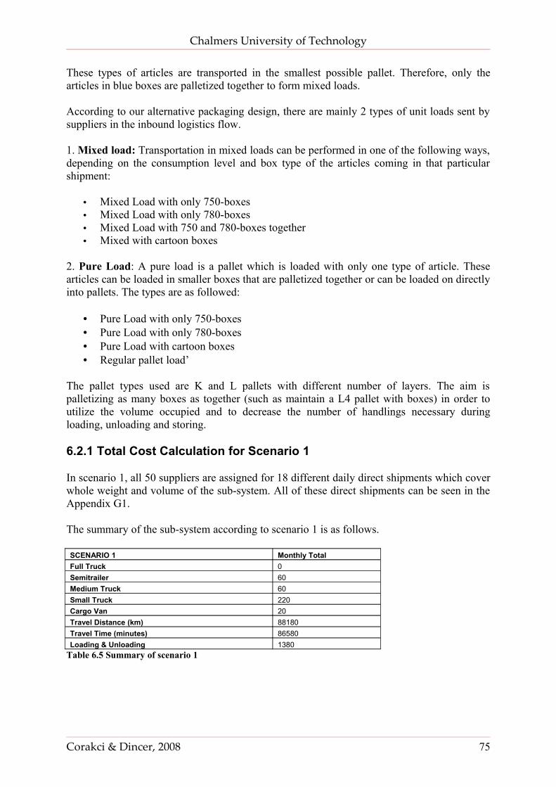
Chalmers University of Technology
These types of articles are transported in the smallest possible pallet. Therefore, only the articles in blue boxes are palletized together to form mixed loads.
According to our alternative packaging design, there are mainly 2 types of unit loads sent by suppliers in the inbound logistics flow.
1. Mixed load: Transportation in mixed loads can be performed in one of the following ways, depending on the consumption level and box type of the articles coming in that particular shipment:
• Mixed Load with only 750-boxes• Mixed Load with only 780-boxes• Mixed Load with 750 and 780-boxes together• Mixed with cartoon boxes
2. Pure Load: A pure load is a pallet which is loaded with only one type of article. These articles can be loaded in smaller boxes that are palletized together or can be loaded on directly into pallets. The types are as followed:
• Pure Load with only 750-boxes• Pure Load with only 780-boxes• Pure Load with cartoon boxes• Regular pallet load’
The pallet types used are K and L pallets with different number of layers. The aim is palletizing as many boxes as together (such as maintain a L4 pallet with boxes) in order to utilize the volume occupied and to decrease the number of handlings necessary during loading, unloading and storing.
6.2.1 Total Cost Calculation for Scenario 1
In scenario 1, all 50 suppliers are assigned for 18 different daily direct shipments which cover whole weight and volume of the sub-system. All of these direct shipments can be seen in the Appendix G1.
The summary of the sub-system according to scenario 1 is as follows.
SCENARIO 1 Monthly TotalFull Truck 0Semitrailer 60Medium Truck 60Small Truck 220Cargo Van 20Travel Distance (km) 88180Travel Time (minutes) 86580Loading & Unloading 1380
Table 6.5 Summary of scenario 1
Corakci & Dincer, 2008 75
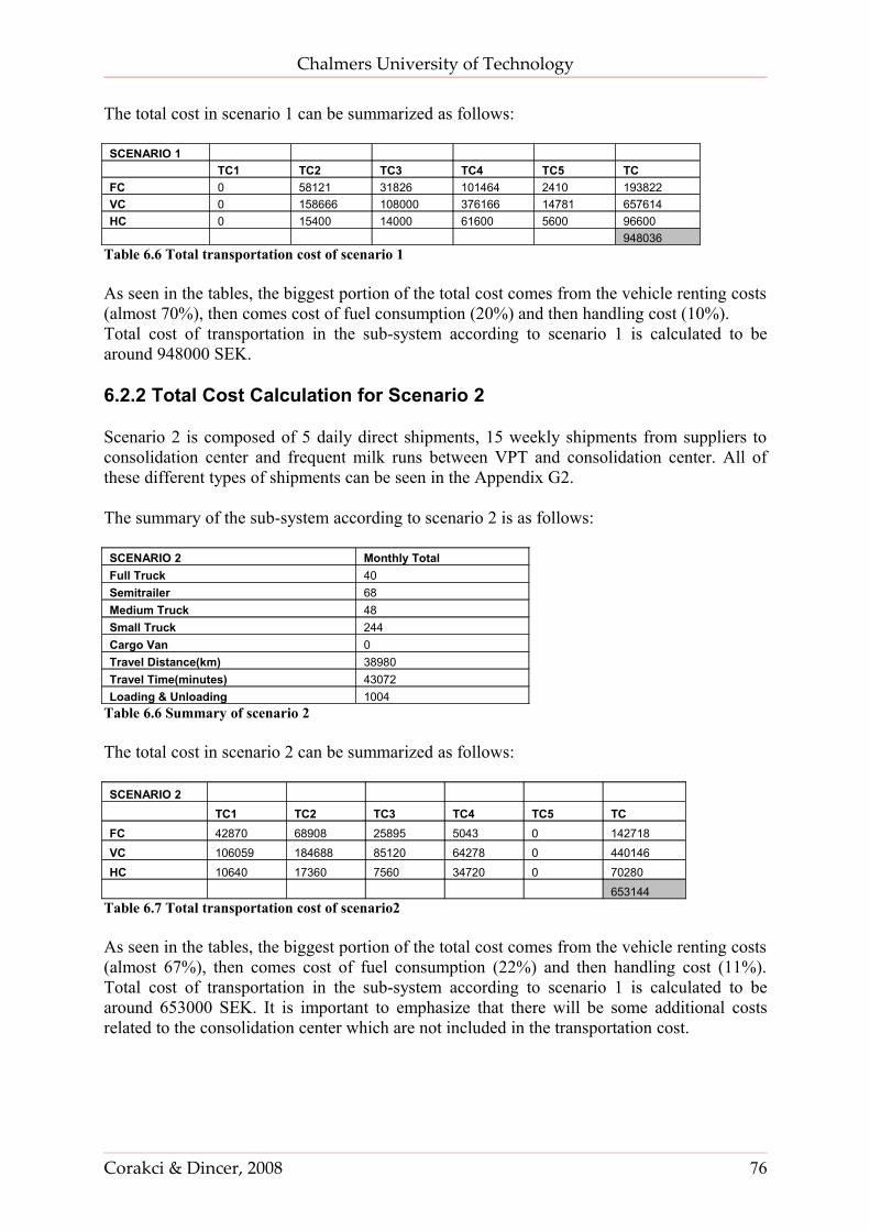
Chalmers University of Technology
The total cost in scenario 1 can be summarized as follows:
SCENARIO 1 TC1 TC2 TC3 TC4 TC5 TCFC 0 58121 31826 101464 2410 193822VC 0 158666 108000 376166 14781 657614HC 0 15400 14000 61600 5600 96600 948036
Table 6.6 Total transportation cost of scenario 1
As seen in the tables, the biggest portion of the total cost comes from the vehicle renting costs (almost 70%), then comes cost of fuel consumption (20%) and then handling cost (10%).Total cost of transportation in the sub-system according to scenario 1 is calculated to be around 948000 SEK.
6.2.2 Total Cost Calculation for Scenario 2
Scenario 2 is composed of 5 daily direct shipments, 15 weekly shipments from suppliers to consolidation center and frequent milk runs between VPT and consolidation center. All of these different types of shipments can be seen in the Appendix G2.
The summary of the sub-system according to scenario 2 is as follows:
SCENARIO 2 Monthly TotalFull Truck 40Semitrailer 68Medium Truck 48Small Truck 244Cargo Van 0Travel Distance(km) 38980Travel Time(minutes) 43072Loading & Unloading 1004
Table 6.6 Summary of scenario 2
The total cost in scenario 2 can be summarized as follows:
SCENARIO 2 TC1 TC2 TC3 TC4 TC5 TCFC 42870 68908 25895 5043 0 142718VC 106059 184688 85120 64278 0 440146HC 10640 17360 7560 34720 0 70280
653144Table 6.7 Total transportation cost of scenario2
As seen in the tables, the biggest portion of the total cost comes from the vehicle renting costs (almost 67%), then comes cost of fuel consumption (22%) and then handling cost (11%). Total cost of transportation in the sub-system according to scenario 1 is calculated to be around 653000 SEK. It is important to emphasize that there will be some additional costs related to the consolidation center which are not included in the transportation cost.
Corakci & Dincer, 2008 76
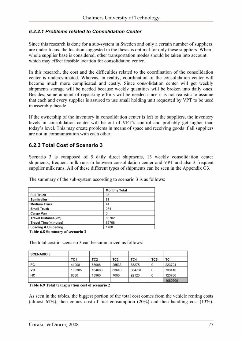
Chalmers University of Technology
6.2.2.1 Problems related to Consolidation Center
Since this research is done for a sub-system in Sweden and only a certain number of suppliers are under focus, the location suggested in the thesis is optimal for only these suppliers. When whole supplier base is considered, other transportation modes should be taken into account which may effect feasible location for consolidation center.
In this research, the cost and the difficulties related to the coordination of the consolidation center is underestimated. Whereas, in reality, coordination of the consolidation center will become much more complicated and costly. Since consolidation center will get weekly shipments storage will be needed because weekly quantities will be broken into daily ones. Besides, some amount of repacking efforts will be needed since it is not realistic to assume that each and every supplier is assured to use small holding unit requested by VPT to be used in assembly façade.
If the ownership of the inventory in consolidation center is left to the suppliers, the inventory levels in consolidation center will be out of VPT’s control and probably get higher than today’s level. This may create problems in means of space and receiving goods if all suppliers are not in communication with each other.
6.2.3 Total Cost of Scenario 3
Scenario 3 is composed of 5 daily direct shipments, 13 weekly consolidation center shipments, frequent milk runs in between consolidation center and VPT and also 3 frequent supplier milk runs. All of these different types of shipments can be seen in the Appendix G3.
The summary of the sub-system according to scenario 3 is as follows:
Monthly TotalFull Truck 36Semitrailer 68Medium Truck 44Small Truck 264Cargo Van 0Travel Distance(km) 86702Travel Time(minutes) 89768Loading & Unloading 1768
Table 6.8 Summary of scenario 3
The total cost in scenario 3 can be summarized as follows:
SCENARIO 3 TC1 TC2 TC3 TC4 TC5 TCFC 41008 68908 25533 88275 0 223724VC 100385 184688 83640 364704 0 733416HC 8680 15960 7000 92120 0 123760 1080900
Table 6.9 Total transpiration cost of scenario 2
As seen in the tables, the biggest portion of the total cost comes from the vehicle renting costs (almost 67%), then comes cost of fuel consumption (20%) and then handling cost (13%).
Corakci & Dincer, 2008 77
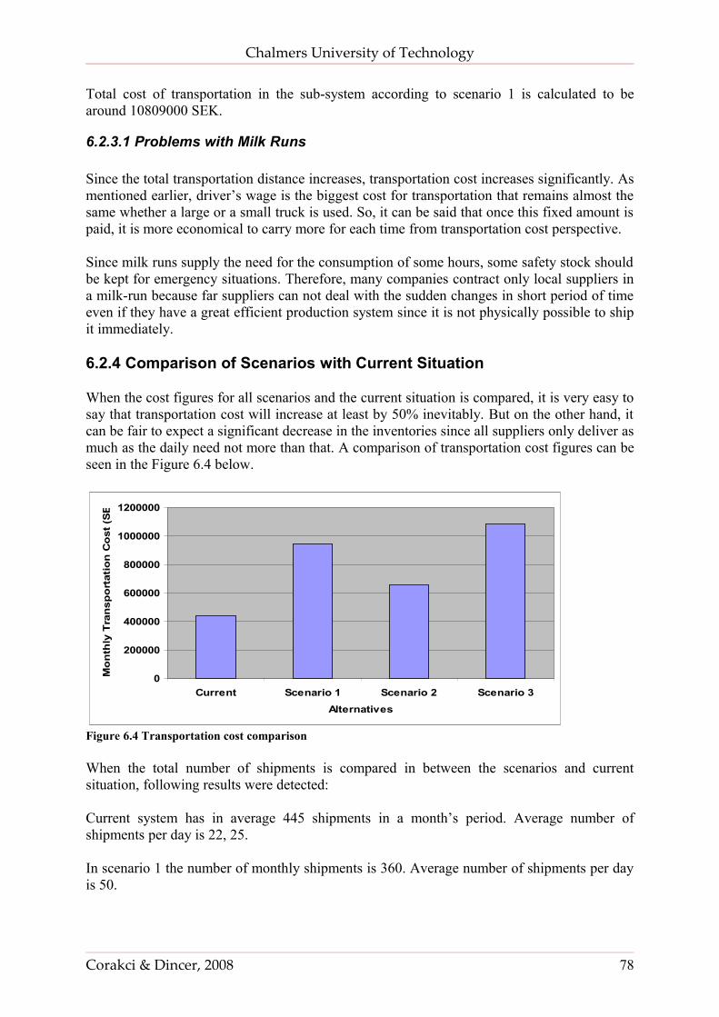
Chalmers University of Technology
Total cost of transportation in the sub-system according to scenario 1 is calculated to be around 10809000 SEK.
6.2.3.1 Problems with Milk Runs
Since the total transportation distance increases, transportation cost increases significantly. As mentioned earlier, driver’s wage is the biggest cost for transportation that remains almost the same whether a large or a small truck is used. So, it can be said that once this fixed amount is paid, it is more economical to carry more for each time from transportation cost perspective.
Since milk runs supply the need for the consumption of some hours, some safety stock should be kept for emergency situations. Therefore, many companies contract only local suppliers in a milk-run because far suppliers can not deal with the sudden changes in short period of time even if they have a great efficient production system since it is not physically possible to ship it immediately.
6.2.4 Comparison of Scenarios with Current Situation
When the cost figures for all scenarios and the current situation is compared, it is very easy to say that transportation cost will increase at least by 50% inevitably. But on the other hand, it can be fair to expect a significant decrease in the inventories since all suppliers only deliver as much as the daily need not more than that. A comparison of transportation cost figures can be seen in the Figure 6.4 below.
0
200000
400000
600000
800000
1000000
1200000
Current Scenario 1 Scenario 2 Scenario 3Alternatives
Mo
nth
ly T
ran
spo
rtat
ion
Co
st (
SE
K)
Figure 6.4 Transportation cost comparison
When the total number of shipments is compared in between the scenarios and current situation, following results were detected:
Current system has in average 445 shipments in a month’s period. Average number of shipments per day is 22, 25.
In scenario 1 the number of monthly shipments is 360. Average number of shipments per day is 50.
Corakci & Dincer, 2008 78
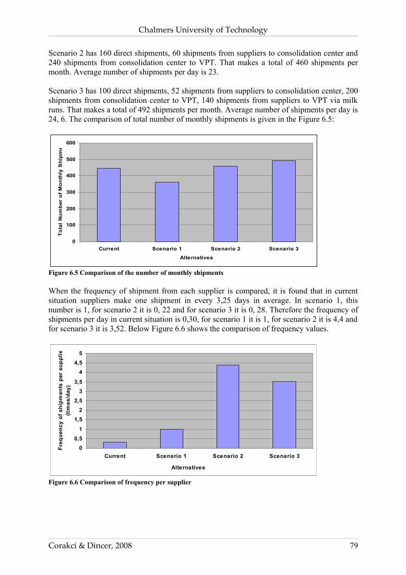
Chalmers University of Technology
Scenario 2 has 160 direct shipments, 60 shipments from suppliers to consolidation center and 240 shipments from consolidation center to VPT. That makes a total of 460 shipments per month. Average number of shipments per day is 23.
Scenario 3 has 100 direct shipments, 52 shipments from suppliers to consolidation center, 200 shipments from consolidation center to VPT, 140 shipments from suppliers to VPT via milk runs. That makes a total of 492 shipments per month. Average number of shipments per day is 24, 6. The comparison of total number of monthly shipments is given in the Figure 6.5:
0
100
200
300
400
500
600
Current Scenario 1 Scenario 2 Scenario 3
Alternatives
To
tal
Nu
mb
er o
f M
on
thly
Sh
ipm
ents
Figure 6.5 Comparison of the number of monthly shipments
When the frequency of shipment from each supplier is compared, it is found that in current situation suppliers make one shipment in every 3,25 days in average. In scenario 1, this number is 1, for scenario 2 it is 0, 22 and for scenario 3 it is 0, 28. Therefore the frequency of shipments per day in current situation is 0,30, for scenario 1 it is 1, for scenario 2 it is 4,4 and for scenario 3 it is 3,52. Below Figure 6.6 shows the comparison of frequency values.
00,5
1
1,52
2,53
3,5
44,5
5
Current Scenario 1 Scenario 2 Scenario 3
Alternatives
Freq
uenc
y of
shi
pmen
ts p
er s
uppl
ier
(ti
mes
/day
)
Figure 6.6 Comparison of frequency per supplier
Corakci & Dincer, 2008 79
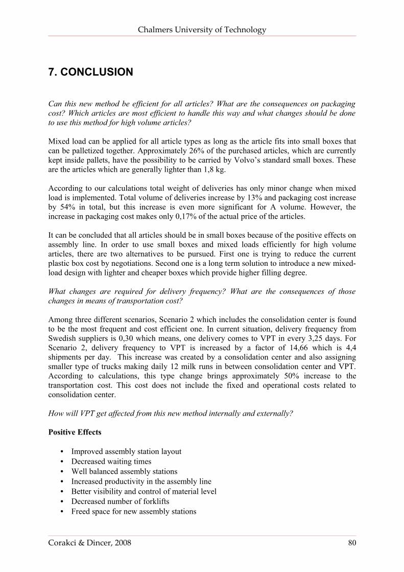
Chalmers University of Technology
7. CONCLUSION
Can this new method be efficient for all articles? What are the consequences on packaging cost? Which articles are most efficient to handle this way and what changes should be done to use this method for high volume articles?
Mixed load can be applied for all article types as long as the article fits into small boxes that can be palletized together. Approximately 26% of the purchased articles, which are currently kept inside pallets, have the possibility to be carried by Volvo’s standard small boxes. These are the articles which are generally lighter than 1,8 kg.
According to our calculations total weight of deliveries has only minor change when mixed load is implemented. Total volume of deliveries increase by 13% and packaging cost increase by 54% in total, but this increase is even more significant for A volume. However, the increase in packaging cost makes only 0,17% of the actual price of the articles.
It can be concluded that all articles should be in small boxes because of the positive effects on assembly line. In order to use small boxes and mixed loads efficiently for high volume articles, there are two alternatives to be pursued. First one is trying to reduce the current plastic box cost by negotiations. Second one is a long term solution to introduce a new mixed-load design with lighter and cheaper boxes which provide higher filling degree.
What changes are required for delivery frequency? What are the consequences of those changes in means of transportation cost?
Among three different scenarios, Scenario 2 which includes the consolidation center is found to be the most frequent and cost efficient one. In current situation, delivery frequency from Swedish suppliers is 0,30 which means, one delivery comes to VPT in every 3,25 days. For Scenario 2, delivery frequency to VPT is increased by a factor of 14,66 which is 4,4 shipments per day. This increase was created by a consolidation center and also assigning smaller type of trucks making daily 12 milk runs in between consolidation center and VPT. According to calculations, this type change brings approximately 50% increase to the transportation cost. This cost does not include the fixed and operational costs related to consolidation center.
How will VPT get affected from this new method internally and externally?
Positive Effects
• Improved assembly station layout• Decreased waiting times• Well balanced assembly stations• Increased productivity in the assembly line• Better visibility and control of material level • Decreased number of forklifts • Freed space for new assembly stations
Corakci & Dincer, 2008 80
Chalmers University of Technology
• Reduced stock levels• Reduced tied-up capital• Opportunity to eliminate high storage and warehouse inside the plant• Eliminated repacking inside the plant• Opportunity to isolate warehousing activities from the plant• Creating a smooth and continuous material flow internally and externally• Opportunity to reveal the problems easier by low stock levels
Negative Effects
• Increased packaging cost• Increased total volume of deliveries• Increased number of material handling• Increased transportation cost• Investment for consolidation center• Difficulties to convince the suppliers for the changes
Corakci & Dincer, 2008 81
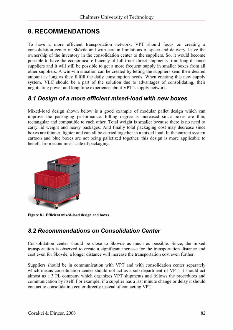
Chalmers University of Technology
8. RECOMMENDATIONS
To have a more efficient transportation network, VPT should focus on creating a consolidation center in Skövde and with certain limitations of space and delivery, leave the ownership of the inventory in the consolidation center to the suppliers. So, it would become possible to have the economical efficiency of full truck direct shipments from long distance suppliers and it will still be possible to get a more frequent supply in smaller boxes from all other suppliers. A win-win situation can be created by letting the suppliers send their desired amount as long as they fulfill the daily consumption needs. When creating this new supply system, VLC should be a part of the solution due to advantages of consolidating, their negotiating power and long time experience about VPT’s supply network.
8.1 Design of a more efficient mixed-load with new boxes
Mixed-load design shown below is a good example of modular pallet design which can improve the packaging performance. Filling degree is increased since boxes are thin, rectangular and compatible to each other. Total weight is smaller because there is no need to carry lid weight and heavy packages. And finally total packaging cost may decrease since boxes are thinner, lighter and can all be carried together in a mixed load. In the current system cartoon and blue boxes are not being palletized together, this design is more applicable to benefit from economies scale of packaging.
Figure 8.1 Efficient mixed-load design and boxes
8.2 Recommendations on Consolidation Center
Consolidation center should be close to Skövde as much as possible. Since, the mixed transportation is observed to create a significant increase for the transportation distance and cost even for Skövde, a longer distance will increase the transportation cost even further.
Suppliers should be in communication with VPT and with consolidation center separately which means consolidation center should not act as a sub-department of VPT, it should act almost as a 3 PL company which organizes VPT shipments and follows the procedures and communication by itself. For example, if a supplier has a last minute change or delay it should contact to consolidation center directly instead of contacting VPT.
Corakci & Dincer, 2008 82
Chalmers University of Technology
Suppliers should be given the ownership of the inventory in the consolidation center with some limitations related to space and time windows they could send.
8.3 Recommendations on Milk Runs
Milk Runs are found to be much more efficient when they are implemented with a consolidation center. Instead of visiting a number of suppliers each and every day, frequent milk runs should be done with a close-by consolidation center.
When there is a supplier which already sends direct and can fill a truck, it should not be changed into a milk run. This never becomes as efficient as before in means of cost.
The suppliers who are further away from 2,5 hrs distance are not found valuable for milk run considering the return trip since milk run is a two way trip. So, it is recommended to focus only on local suppliers who cannot fill a full truck themselves.
VPT should not underestimate the advantage of consolidating taken by VLC by delivering for all Volvo group companies together. Creating a VPT specific solution organized by VPT itself, results certainly with higher transportation costs, and probably with a lot of administration problems since VPT does not have long tradition nor the expertise about transporting system solutions. Therefore, a 3PL company should always be involved in the solution.
8.4 Recommendations for Future Research
Some recommendations for future research are identified as follows:
• This study is done for Swedish suppliers only. In order to be able to justify the cost of consolidation center, all suppliers should be taken into consideration.
• Alternative packaging types and mixed load designs should be further investigated and tested.
• Transportation techniques in small boxes without any wooden pallets should be investigated.
• Cost related to this type of researches should be taken into consideration from a total cost point of view. Trade-offs between production, inventory and transportation should be investigated.
Corakci & Dincer, 2008 83
Chalmers University of Technology
REFERENCE LIST
Alina, Tunović. The Coordination of Inbound Logistics Flows: A Case Study of Terms Delivery for the Supply of Components from External Suppliers to SKF Factories, Gothenburg University, 2003.
Balintfy, J.L. On the Basic Class of Multi-Item Inventory Problems, Management Science: 10, 1964.
Baudin, Michel. Lean Logistics: The Nuts and Bolts of Delivering Materials and Goods, New York: Productivity Press, 2004.
Bicheno, John. The New Lean Toolbox: Towards Fast, Flexible Flow, PICSIE Books1998.
Bowersox, Closs and Cooper. Supply Chain Logistics Management, McGraw-Hill, 2002.
Chan, F.T.S and H.K. Chan. A Systematic Approach to Manufacturing Packaging Logistics, International Journal of Advanced Manufacturing Technology 29, 2006.
Cimorelli, Stephen C. Kanban for the Supply Chain: Fundamental Practices for Manufacturing Management, 2005. Productivity Press.
Cooke, James Aaron. Should You Control Your Inbound, Traffic Management 32, 1993.
Coyle, Bardi and Langley. The Management of Business Logistics, MN: West Publishing, 1996.
Elvander, Ståhl. A Theoretical Mapping of VMI Concept, Lund University, 2005.
Eriksson, Pär and Eva Meding. Importance of Transportation Costs for Industrial Restructuring Projects at Nestle, Chalmers University of Technology, 2000.
Finnsgård, Christian. The Impact of Materials Exposure on the Performance at the Point-of-Use, Göteborg, Division of Logistics and Transportation, 2008.
Grimshorn, Peter and Svante Karlsson. VMI at Volvo Truck Corporation: An Evaluation of the Possibility to Implement VMI to Control Inbound Logistics to Volvo Truck's Assembly Factories in Tuve and Gent, Chalmers University of Technology, 2006.
Gummesson, E. All Research Is Interpretive, Journal of Business and Industrial Marketing 18, 482-92, 2003.
Harrison, Alan and Remko Van Hoek. Logistics Management and Strategy, Essex: Pearson Education, 2005.
Johansson, Kennert and Ann Lorentzon Karlsson. Packaging Logistics, Stockholm: Packforsk, 1997.
Johansson, Kennert and Pär Weström. Measurement of Packaging Logistics Parameters, Packaging Logistics Review, 2000.
Corakci & Dincer, 2008 84
Chalmers University of Technology
Jonsson, Patrik and Stig Arne Mattsson. Production and Materials Management, Gothenburg: Chalmers University of Technology, 2007.
Kozussek, Kevin. Mixed-Load Palletizing: Supply Chain Economics, 2005.
Kumar, S.A. Production & Operations Management, New Age International Ltd, 2006.
Liker, Jeffrey K. The Toyota Way: 14 Management Principles from the World's Greatest Manufacturer, New York: McGraw Hill, 2004.
Lumsden, Kenth. Complete Fundamentals of Logistics, Gothenburg: Chalmers University of Technology, 2002.
Management, Indian Institute of Materials. In-Plant Logistics: Key to the Success of a Lean Enterprise, 2008. </knowledge_bank/1_in-plant-logistics-key-tothe-success-of-leanenterprises.htm>.
Mills, Patricia Nemetz. Operations Management Focusing on Quality & Competitiveness Facility Location, 2008. <http://www.cbpa.ewu.edu/~pnemetzmills/OMch5s/outline.html>.
Morabito, Reinaldo and Silvia Regina Morales. Loading Optimization of Palletized Products on Trucks, Transportation Research Part E, 2000.
Nicholas, John and Avi Soni. The Portal to Lean Production: Principles and Practices for Doing More with Less, New York: Auerbach Publications, 2006.
Nicholas, John M. Competitive Manufacturing Management, Singapore: McGraw Hill, 1998.
Stake, R. The Art of Case Research, Newbury Park, CA: Sage Publications, 1995.
Stock, James and Douglas Lambert. Strategic Logistics Management, New York: McGraw-Hill, 2001.
Suzaki, Kiyoshi. The New Manufacturing Challenge: Techniques for Continuous Improvement, New York: Free Press, 1987.
Teulings and Vlist. Managing the Supply Chain with Standard Mixed Loads, International Journal of Physical Distribution & Logistics 31, 2001.
Torstensson, Håkan and Göran Stjernman. Packaging and Cargo Carrier Technology. Borås: University College of Borås, 2006.
Womack, P.and D. Jones. The Machine That Changed the World: The Story of Lean Production, Cambridge: MIT Press, 1990.
Womack, P.and D. Jones. Lean Thinking: Banish Waste and Create Wealth in Your Corporation, New York: Simon & Schuster, 1996.
Yamashina, Hajime. Logistics Concepts, Royal Swedish Academy of Engineering Sciences, 2006.
Corakci & Dincer, 2008 85
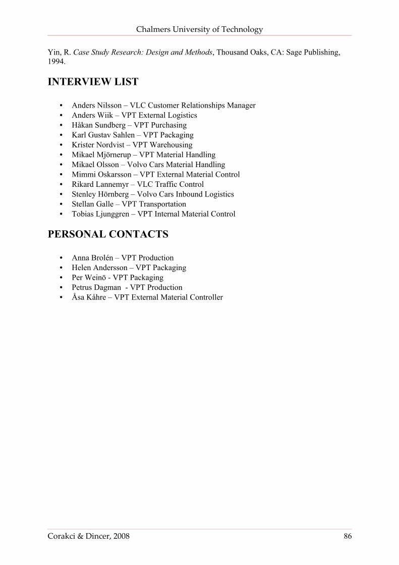
Chalmers University of Technology
Yin, R. Case Study Research: Design and Methods, Thousand Oaks, CA: Sage Publishing, 1994.
INTERVIEW LIST
• Anders Nilsson – VLC Customer Relationships Manager• Anders Wiik – VPT External Logistics • Håkan Sundberg – VPT Purchasing• Karl Gustav Sahlen – VPT Packaging• Krister Nordvist – VPT Warehousing• Mikael Mjörnerup – VPT Material Handling• Mikael Olsson – Volvo Cars Material Handling• Mimmi Oskarsson – VPT External Material Control• Rikard Lannemyr – VLC Traffic Control• Stenley Hörnberg – Volvo Cars Inbound Logistics• Stellan Galle – VPT Transportation• Tobias Ljunggren – VPT Internal Material Control
PERSONAL CONTACTS
• Anna Brolén – VPT Production• Helen Andersson – VPT Packaging• Per Weinö - VPT Packaging• Petrus Dagman - VPT Production• Åsa Kåhre – VPT External Material Controller
Corakci & Dincer, 2008 86
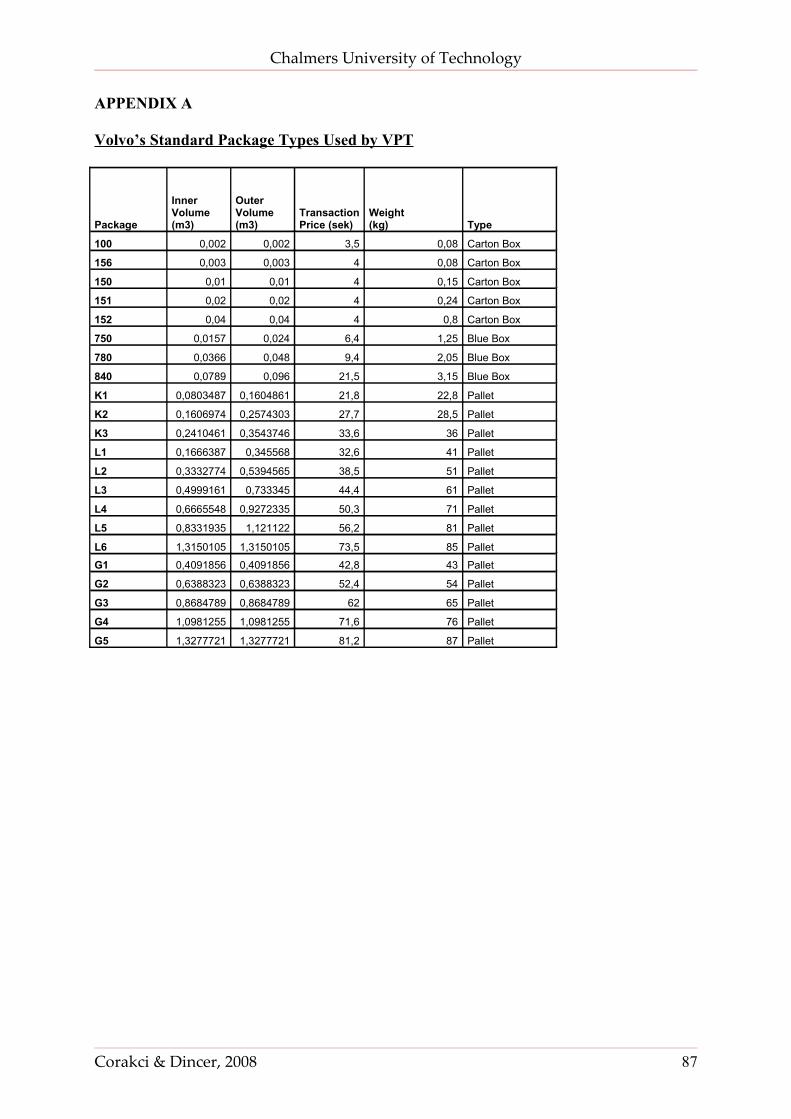
Chalmers University of Technology
APPENDIX A
Volvo’s Standard Package Types Used by VPT
Package
InnerVolume(m3)
Outer Volume(m3)
Transaction Price (sek)
Weight(kg) Type
100 0,002 0,002 3,5 0,08 Carton Box
156 0,003 0,003 4 0,08 Carton Box
150 0,01 0,01 4 0,15 Carton Box
151 0,02 0,02 4 0,24 Carton Box
152 0,04 0,04 4 0,8 Carton Box
750 0,0157 0,024 6,4 1,25 Blue Box
780 0,0366 0,048 9,4 2,05 Blue Box
840 0,0789 0,096 21,5 3,15 Blue Box
K1 0,0803487 0,1604861 21,8 22,8 Pallet
K2 0,1606974 0,2574303 27,7 28,5 Pallet
K3 0,2410461 0,3543746 33,6 36 Pallet
L1 0,1666387 0,345568 32,6 41 Pallet
L2 0,3332774 0,5394565 38,5 51 Pallet
L3 0,4999161 0,733345 44,4 61 Pallet
L4 0,6665548 0,9272335 50,3 71 Pallet
L5 0,8331935 1,121122 56,2 81 Pallet
L6 1,3150105 1,3150105 73,5 85 Pallet
G1 0,4091856 0,4091856 42,8 43 Pallet
G2 0,6388323 0,6388323 52,4 54 Pallet
G3 0,8684789 0,8684789 62 65 Pallet
G4 1,0981255 1,0981255 71,6 76 Pallet
G5 1,3277721 1,3277721 81,2 87 Pallet
Corakci & Dincer, 2008 87
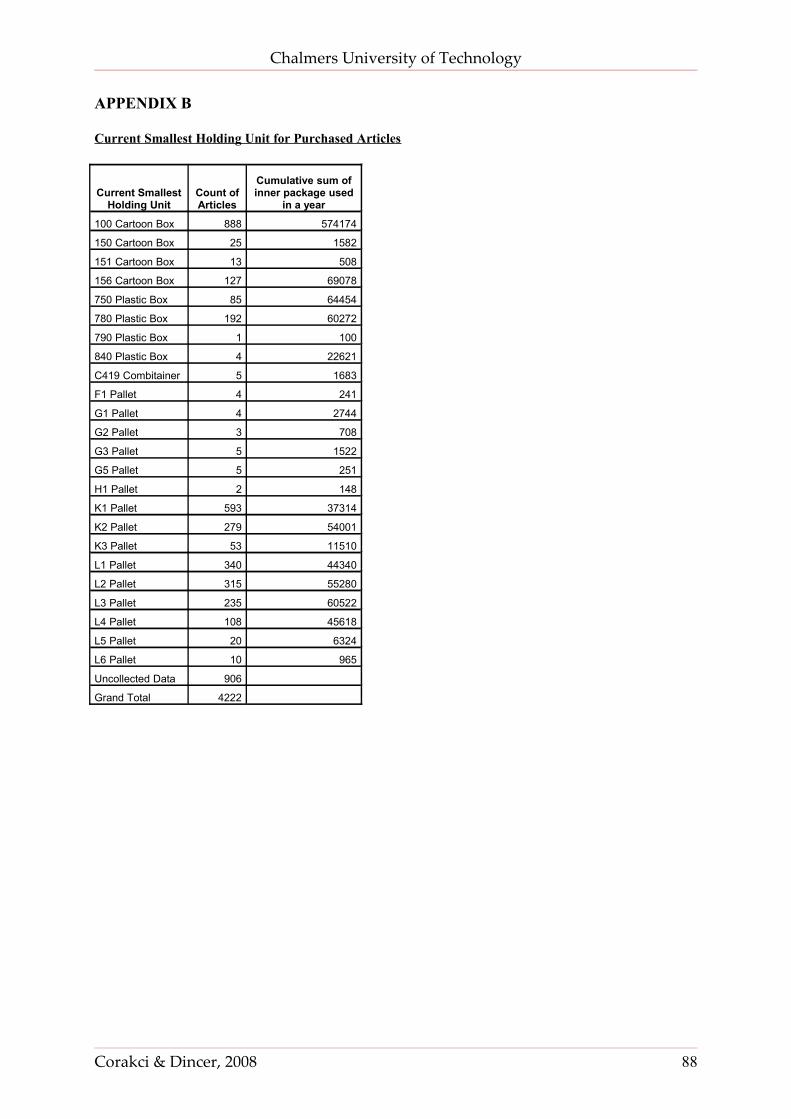
Chalmers University of Technology
APPENDIX B
Current Smallest Holding Unit for Purchased Articles
Current Smallest Holding Unit
Count of Articles
Cumulative sum of inner package used
in a year
100 Cartoon Box 888 574174
150 Cartoon Box 25 1582
151 Cartoon Box 13 508
156 Cartoon Box 127 69078
750 Plastic Box 85 64454
780 Plastic Box 192 60272
790 Plastic Box 1 100
840 Plastic Box 4 22621
C419 Combitainer 5 1683
F1 Pallet 4 241
G1 Pallet 4 2744
G2 Pallet 3 708
G3 Pallet 5 1522
G5 Pallet 5 251
H1 Pallet 2 148
K1 Pallet 593 37314
K2 Pallet 279 54001
K3 Pallet 53 11510
L1 Pallet 340 44340
L2 Pallet 315 55280
L3 Pallet 235 60522
L4 Pallet 108 45618
L5 Pallet 20 6324
L6 Pallet 10 965
Uncollected Data 906
Grand Total 4222
Corakci & Dincer, 2008 88
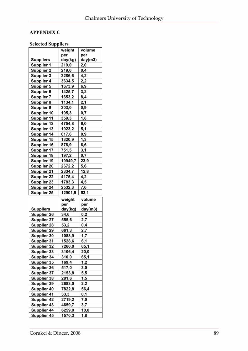
Chalmers University of Technology
APPENDIX C
Selected Suppliers
Suppliers
weight per day(kg)
volume per day(m3)
Supplier 26 34,6 0,2Supplier 27 555,6 2,7Supplier 28 53,2 0,4Supplier 29 661,3 2,7Supplier 30 1088,9 1,7Supplier 31 1528,6 6,1Supplier 32 7260,0 65,1Supplier 33 3106,4 20,0Supplier 34 310,0 65,1Supplier 35 169,4 1,2Supplier 36 517,0 3,0Supplier 37 2153,8 5,5Supplier 38 281,6 1,5Supplier 39 2683,0 2,2Supplier 40 7822,8 56,4Supplier 41 33,3 0,1Supplier 42 2719,2 7,0Supplier 43 4659,7 3,7Supplier 44 6259,0 10,0Supplier 45 1570,3 1,8
Corakci & Dincer, 2008 89
Suppliers
weight per day(kg)
volume per day(m3)
Supplier 1 219,0 2,0Supplier 2 219,0 0,4Supplier 3 2286,6 4,2Supplier 4 3634,5 2,2Supplier 5 1673,9 6,9Supplier 6 1425,7 3,2Supplier 7 1653,2 8,4Supplier 8 1134,1 2,1Supplier 9 203,0 0,9Supplier 10 195,3 0,7Supplier 11 359,3 1,8Supplier 12 4754,8 6,0Supplier 13 1923,2 5,1Supplier 14 617,6 0,9Supplier 15 1320,9 1,3Supplier 16 878,9 6,6Supplier 17 751,5 3,1Supplier 18 197,2 0,7Supplier 19 19949,7 23,9Supplier 20 2672,2 5,6Supplier 21 2334,7 12,8Supplier 22 4175,4 4,2Supplier 23 1783,3 4,5Supplier 24 2532,3 7,0Supplier 25 12901,9 53,1
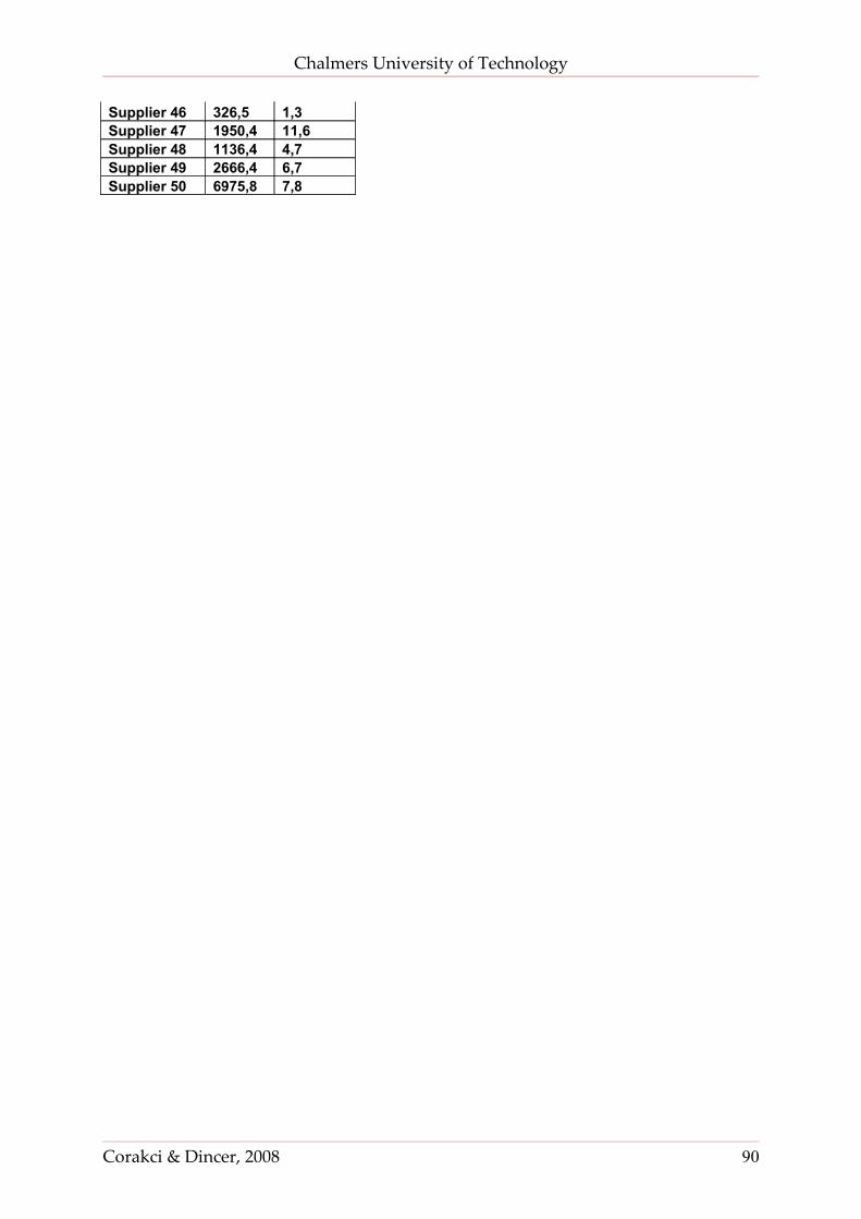
Chalmers University of Technology
Supplier 46 326,5 1,3Supplier 47 1950,4 11,6Supplier 48 1136,4 4,7Supplier 49 2666,4 6,7Supplier 50 6975,8 7,8
Corakci & Dincer, 2008 90
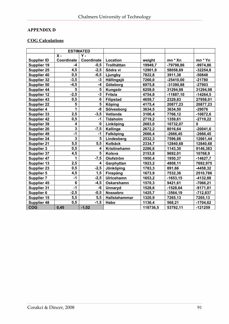
Chalmers University of Technology
APPENDIX D
COG Calculations
ESTIMATED
Supplier IDX - Coordinate
Y - Coordinate Location weight mn * Xn mn * Yn
Supplier 19 -4 -0,5 Trollhättan 19949,7 -79798,86 -9974,86Supplier 25 4,5 -2,5 Södra vi 12901,9 58058,69 -32254,8Supplier 40 0,5 -6,5 Ljungby 7822,8 3911,38 -50848Supplier 32 -3,5 -3 Hällingsjö 7260,0 -25410,00 -21780Supplier 50 -4,5 -4 Göteborg 6975,8 -31390,88 -27903Supplier 44 5 5 Kungsör 6259,0 31294,98 31294,98Supplier 12 -2,5 -3 Fritsla 4754,8 -11887,10 -14264,5Supplier 43 0,5 6 Filipstad 4659,7 2329,83 27958,01Supplier 22 5 5 Köping 4175,4 20877,23 20877,23Supplier 4 1 -8 Sölvesborg 3634,5 3634,50 -29076Supplier 33 2,5 -3,5 Vetlanda 3106,4 7766,12 -10872,6Supplier 42 0,5 -1 Tidaholm 2719,2 1359,61 -2719,22Supplier 39 4 0 Linköping 2683,0 10732,07 0Supplier 20 3 -7,5 Kallinge 2672,2 8016,64 -20041,6Supplier 49 -1 -1 Falköping 2666,4 -2666,45 -2666,45Supplier 24 3 5 Lindesberg 2532,3 7596,86 12661,44Supplier 21 5,5 5,5 Kolbäck 2334,7 12840,68 12840,68Supplier 3 0,5 4 Kristinehamn 2286,6 1143,30 9146,383Supplier 37 4,5 5 Kolsva 2153,8 9692,01 10768,9Supplier 47 1 -7,5 Olofström 1950,4 1950,37 -14627,7Supplier 13 2,5 4 Garphyttan 1923,2 4808,11 7692,975Supplier 23 0,5 -2,5 Jönköping 1783,3 891,66 -4458,32Supplier 5 4,5 1,5 Finspång 1673,9 7532,36 2510,786Supplier 7 -1 -2,5 Ulricehamn 1653,2 -1653,15 -4132,88Supplier 45 6 -4,5 Oskarshamn 1570,3 9421,61 -7066,21Supplier 31 -1 -6 Unnaryd 1528,6 -1528,64 -9171,81Supplier 6 -2,5 -0,5 Nossebro 1425,7 -3564,19 -712,837Supplier 15 5,5 5,5 Hallstahammar 1320,9 7265,13 7265,13Supplier 48 0,5 -1,5 Habo 1136,4 568,21 -1704,62COG 0,45 -1,02 118736,5 53792,11 -121259
Corakci & Dincer, 2008 91
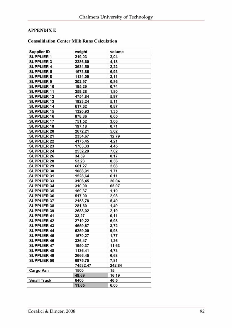
Chalmers University of Technology
APPENDIX E
Consolidation Center Milk Runs Calculation
Supplier ID weight volumeSUPPLIER 1 219,03 2,04SUPPLIER 3 2286,60 4,18SUPPLIER 4 3634,50 2,22SUPPLIER 5 1673,86 6,93SUPPLIER 8 1134,09 2,11SUPPLIER 9 202,97 0,86SUPPLIER 10 195,29 0,74SUPPLIER 11 359,28 1,80SUPPLIER 12 4754,84 5,97SUPPLIER 13 1923,24 5,11SUPPLIER 14 617,62 0,87SUPPLIER 15 1320,93 1,35SUPPLIER 16 878,86 6,65SUPPLIER 17 751,52 3,06SUPPLIER 18 197,18 0,71SUPPLIER 20 2672,21 5,62SUPPLIER 21 2334,67 12,79SUPPLIER 22 4175,45 4,21SUPPLIER 23 1783,33 4,45SUPPLIER 24 2532,29 7,02SUPPLIER 26 34,59 0,17SUPPLIER 28 53,23 0,36SUPPLIER 29 661,27 2,68SUPPLIER 30 1088,91 1,71SUPPLIER 31 1528,64 6,11SUPPLIER 33 3106,45 20,04SUPPLIER 34 310,00 65,07SUPPLIER 35 169,37 1,19SUPPLIER 36 517,00 2,98SUPPLIER 37 2153,78 5,49SUPPLIER 38 281,60 1,49SUPPLIER 39 2683,02 2,19SUPPLIER 41 33,27 0,11SUPPLIER 42 2719,22 6,98SUPPLIER 43 4659,67 3,72SUPPLIER 44 6259,00 9,98SUPPLIER 45 1570,27 1,77SUPPLIER 46 326,47 1,26SUPPLIER 47 1950,37 11,63SUPPLIER 48 1136,41 4,73SUPPLIER 49 2666,45 6,68SUPPLIER 50 6975,75 7,81 74532,47 242,84Cargo Van 1500 15 49,69 16,19Small Truck 6400 40,5 11,65 6,00
Corakci & Dincer, 2008 92
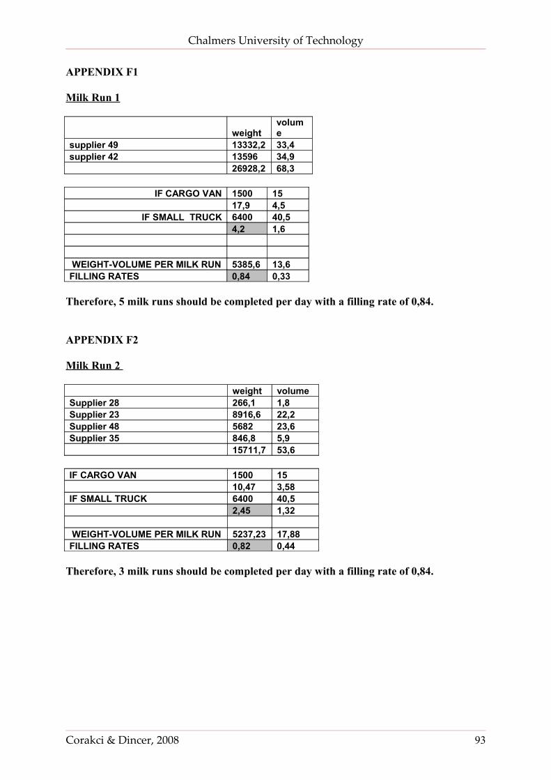
Chalmers University of Technology
APPENDIX F1
Milk Run 1
weightvolume
supplier 49 13332,2 33,4supplier 42 13596 34,9 26928,2 68,3
IF CARGO VAN 1500 15 17,9 4,5
IF SMALL TRUCK 6400 40,5 4,2 1,6 WEIGHT-VOLUME PER MILK RUN 5385,6 13,6FILLING RATES 0,84 0,33
Therefore, 5 milk runs should be completed per day with a filling rate of 0,84.
APPENDIX F2
Milk Run 2
weight volumeSupplier 28 266,1 1,8Supplier 23 8916,6 22,2Supplier 48 5682 23,6Supplier 35 846,8 5,9 15711,7 53,6
IF CARGO VAN 1500 15 10,47 3,58IF SMALL TRUCK 6400 40,5 2,45 1,32 WEIGHT-VOLUME PER MILK RUN 5237,23 17,88FILLING RATES 0,82 0,44
Therefore, 3 milk runs should be completed per day with a filling rate of 0,84.
Corakci & Dincer, 2008 93
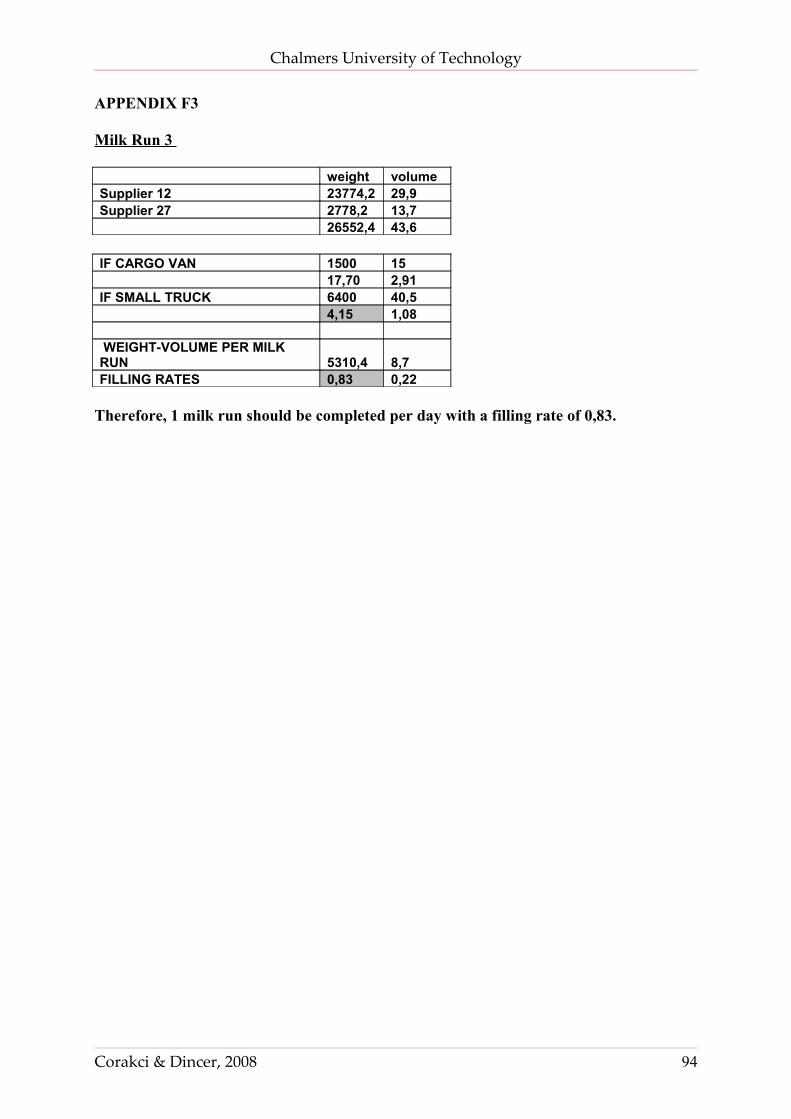
Chalmers University of Technology
APPENDIX F3
Milk Run 3
weight volumeSupplier 12 23774,2 29,9Supplier 27 2778,2 13,7 26552,4 43,6
IF CARGO VAN 1500 15 17,70 2,91IF SMALL TRUCK 6400 40,5 4,15 1,08 WEIGHT-VOLUME PER MILK RUN 5310,4 8,7FILLING RATES 0,83 0,22
Therefore, 1 milk run should be completed per day with a filling rate of 0,83.
Corakci & Dincer, 2008 94
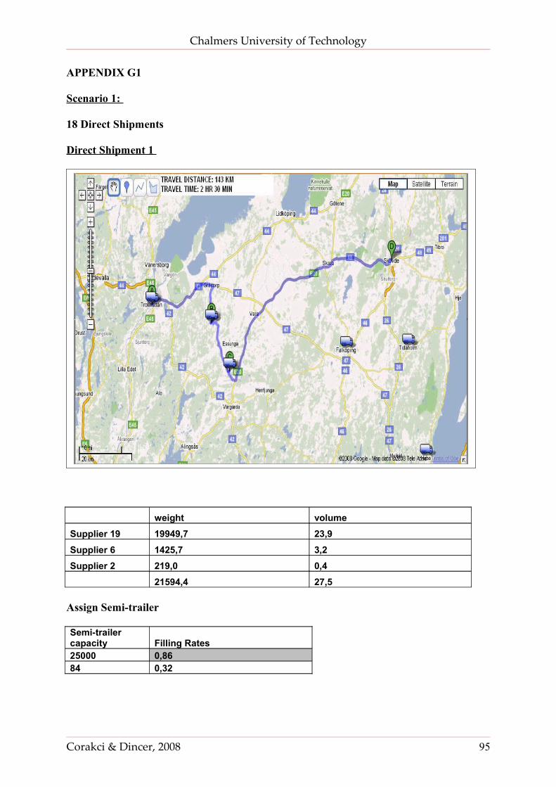
Chalmers University of Technology
APPENDIX G1
Scenario 1:
18 Direct Shipments
Direct Shipment 1
weight volumeSupplier 19 19949,7 23,9Supplier 6 1425,7 3,2Supplier 2 219,0 0,4 21594,4 27,5
Assign Semi-trailer
Semi-trailer capacity Filling Rates25000 0,8684 0,32
Corakci & Dincer, 2008 95
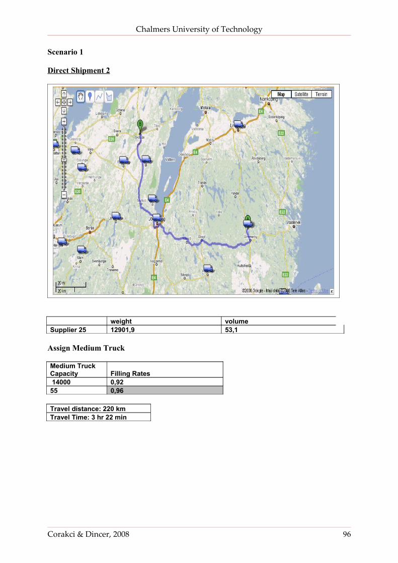
Chalmers University of Technology
Scenario 1
Direct Shipment 2
weight volumeSupplier 25 12901,9 53,1
Assign Medium Truck
Medium Truck Capacity Filling Rates 14000 0,9255 0,96
Travel distance: 220 kmTravel Time: 3 hr 22 min
Corakci & Dincer, 2008 96
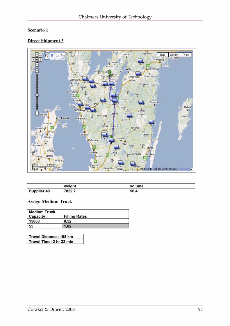
Chalmers University of Technology
Scenario 1
Direct Shipment 3
weight volumeSupplier 40 7822,7 56,4
Assign Medium Truck
Medium Truck Capacity Filling Rates15000 0,5255 1,02
Travel Distance: 198 kmTravel Time: 2 hr 32 min
Corakci & Dincer, 2008 97
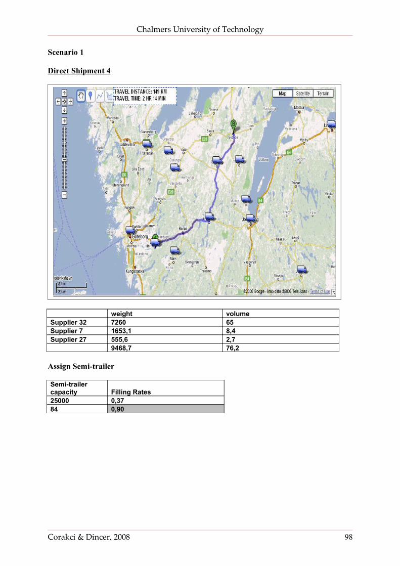
Chalmers University of Technology
Scenario 1
Direct Shipment 4
weight volumeSupplier 32 7260 65Supplier 7 1653,1 8,4Supplier 27 555,6 2,7 9468,7 76,2
Assign Semi-trailer
Semi-trailer capacity Filling Rates25000 0,3784 0,90
Corakci & Dincer, 2008 98
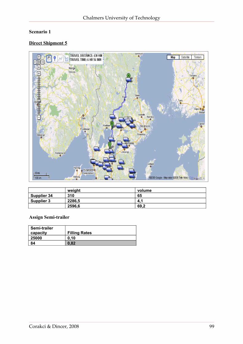
Chalmers University of Technology
Scenario 1
Direct Shipment 5
weight volumeSupplier 34 310 65Supplier 3 2286,5 4,1 2596,6 69,2
Assign Semi-trailer
Semi-trailer capacity Filling Rates25000 0,1084 0,82
Corakci & Dincer, 2008 99
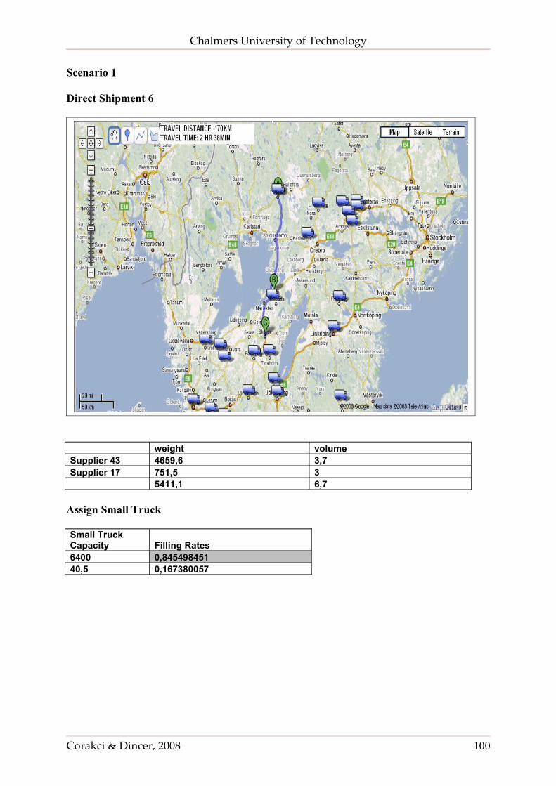
Chalmers University of Technology
Scenario 1
Direct Shipment 6
weight volumeSupplier 43 4659,6 3,7Supplier 17 751,5 3 5411,1 6,7
Assign Small Truck
Small Truck Capacity Filling Rates6400 0,84549845140,5 0,167380057
Corakci & Dincer, 2008 100
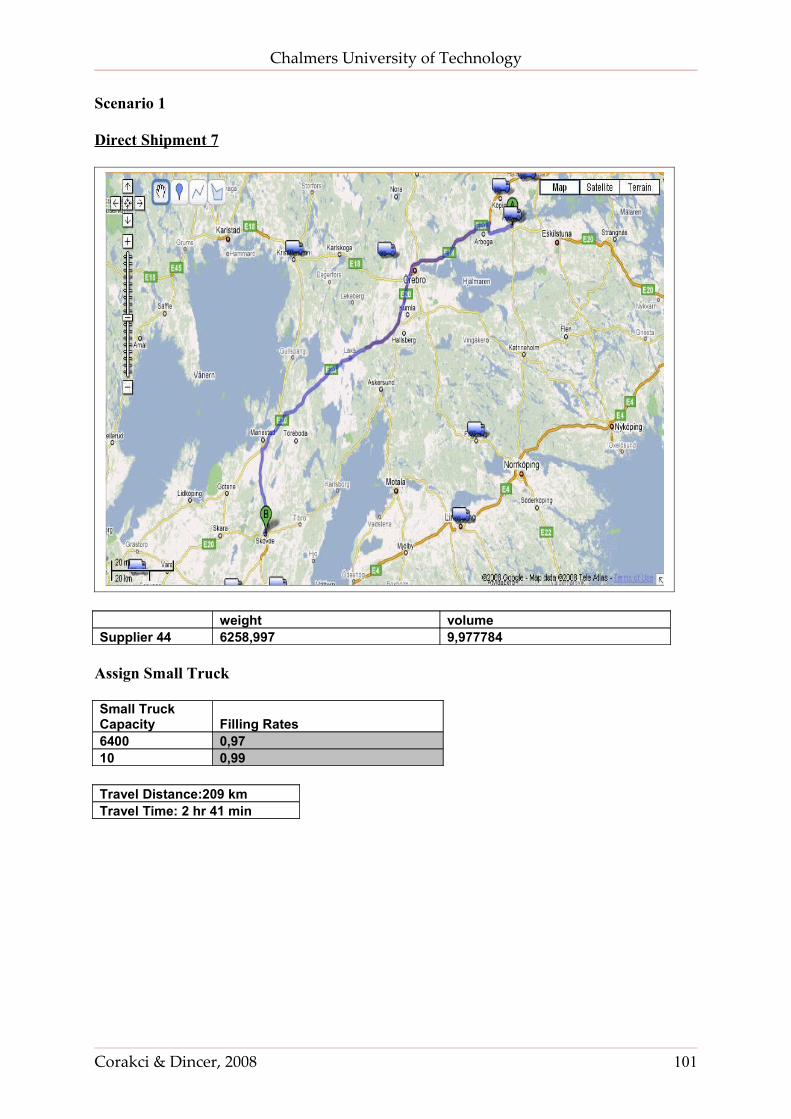
Chalmers University of Technology
Scenario 1
Direct Shipment 7
weight volumeSupplier 44 6258,997 9,977784
Assign Small Truck
Small Truck Capacity Filling Rates6400 0,9710 0,99
Travel Distance:209 kmTravel Time: 2 hr 41 min
Corakci & Dincer, 2008 101
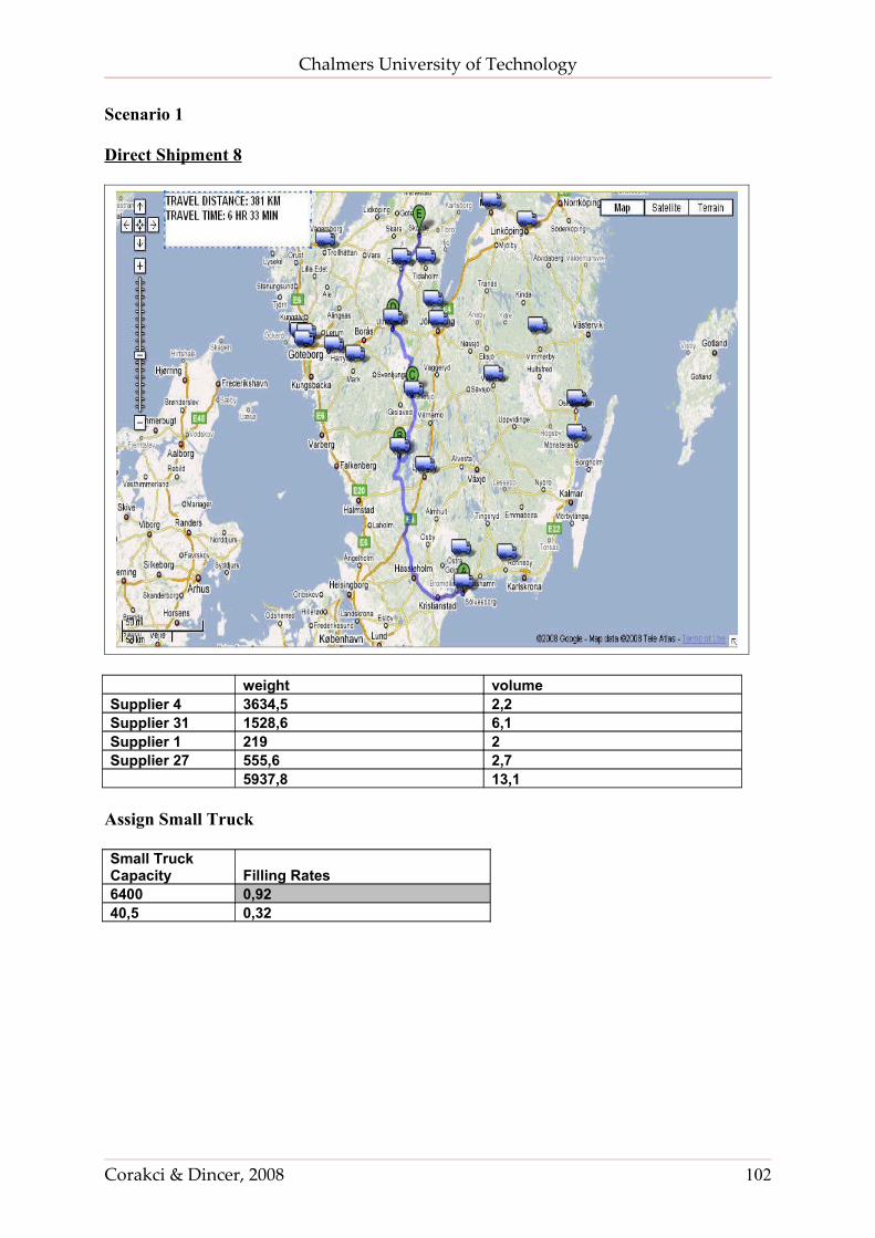
Chalmers University of Technology
Scenario 1
Direct Shipment 8
weight volumeSupplier 4 3634,5 2,2Supplier 31 1528,6 6,1Supplier 1 219 2Supplier 27 555,6 2,7 5937,8 13,1
Assign Small Truck
Small Truck Capacity Filling Rates6400 0,9240,5 0,32
Corakci & Dincer, 2008 102
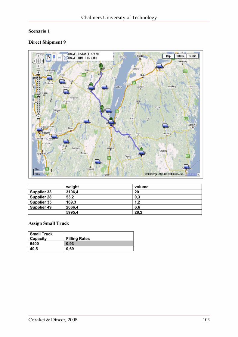
Chalmers University of Technology
Scenario 1
Direct Shipment 9
weight volumeSupplier 33 3106,4 20Supplier 28 53,2 0,3Supplier 35 169,3 1,2Supplier 49 2666,4 6,6 5995,4 28,2
Assign Small Truck
Small Truck Capacity Filling Rates6400 0,9340,5 0,69
Corakci & Dincer, 2008 103

Chalmers University of Technology
Scenario 1
Direct Shipment 10
weight volumeSupplier 5 1673,8 6,9Supplier 39 2683 2,2Supplier 16 878,8 6,6Supplier 41 33,2 0,1Supplier 38 281,6 1,5 5269 17,3
Assign Small Truck
Small Truck Capacity Filling Rates6400 0,8240,5 0,42
Corakci & Dincer, 2008 104
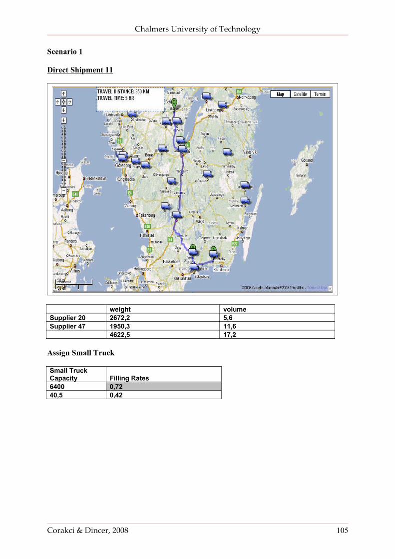
Chalmers University of Technology
Scenario 1
Direct Shipment 11
weight volumeSupplier 20 2672,2 5,6Supplier 47 1950,3 11,6 4622,5 17,2
Assign Small Truck
Small Truck Capacity Filling Rates6400 0,7240,5 0,42
Corakci & Dincer, 2008 105
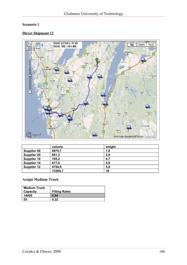
Chalmers University of Technology
Scenario 1
Direct Shipment 12
volume weightSupplier 50 6975,7 7,8Supplier 29 661,2 2,6Supplier 10 195,2 0,7Supplier 14 617,6 0,8Supplier 12 4754,8 5,9 13204,7 18
Assign Medium Truck
Medium Truck Capacity Filling Rates14000 0,9455 0,32
Corakci & Dincer, 2008 106
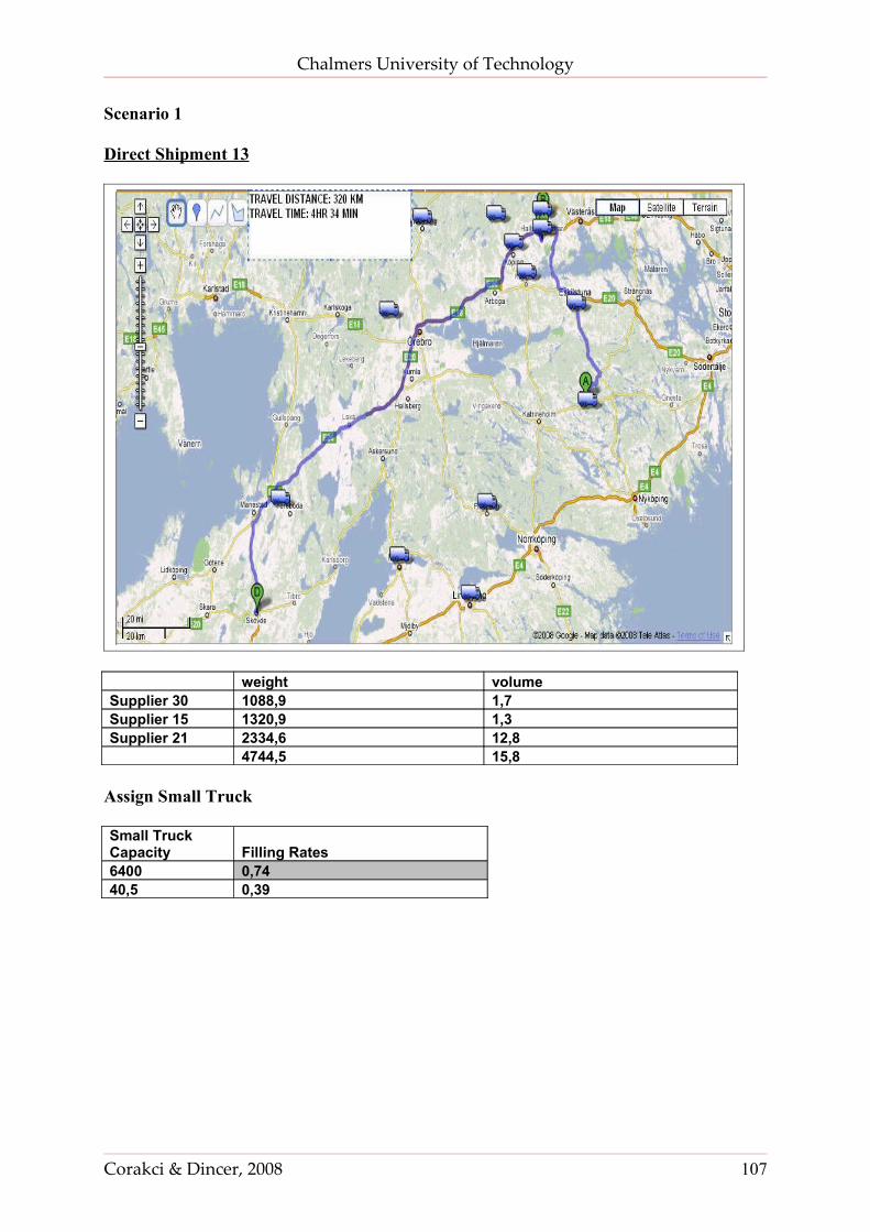
Chalmers University of Technology
Scenario 1
Direct Shipment 13
weight volumeSupplier 30 1088,9 1,7Supplier 15 1320,9 1,3Supplier 21 2334,6 12,8 4744,5 15,8
Assign Small Truck
Small Truck Capacity Filling Rates6400 0,7440,5 0,39
Corakci & Dincer, 2008 107
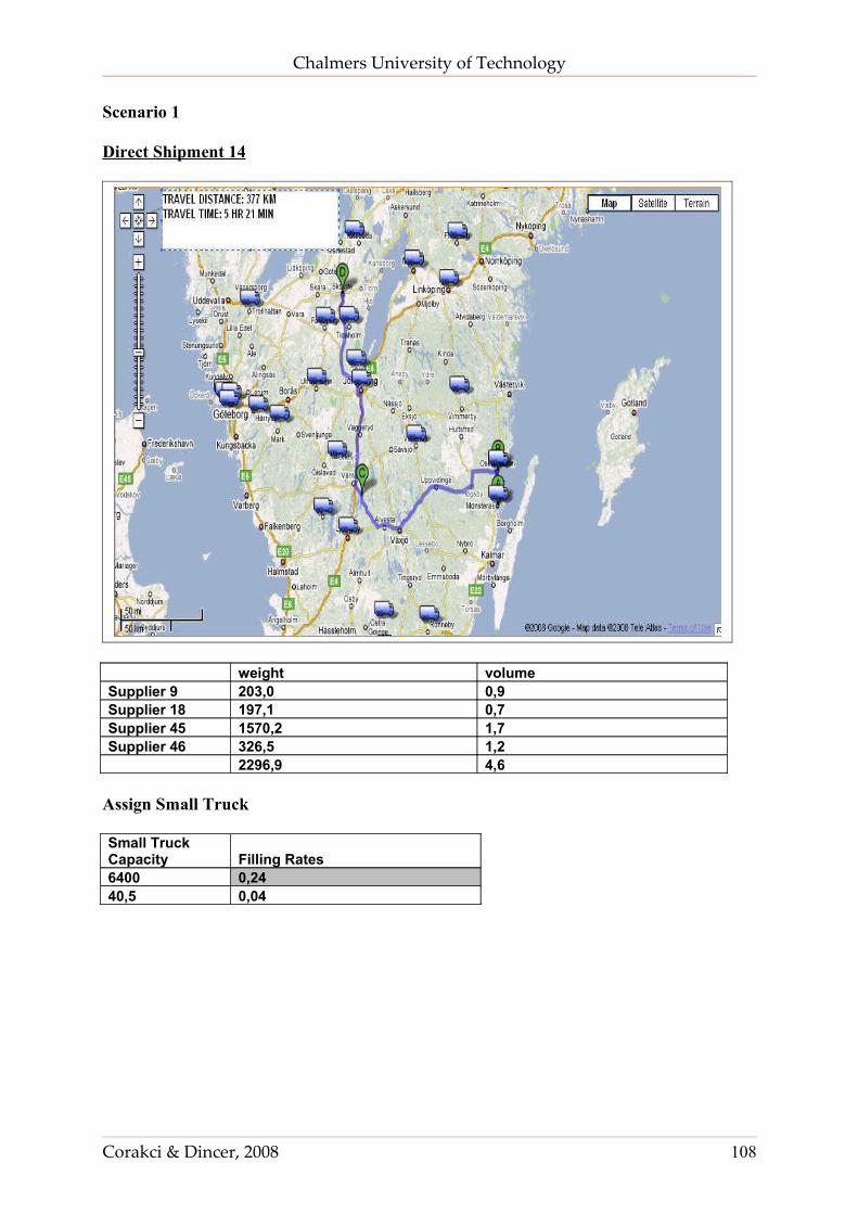
Chalmers University of Technology
Scenario 1
Direct Shipment 14
weight volumeSupplier 9 203,0 0,9Supplier 18 197,1 0,7Supplier 45 1570,2 1,7Supplier 46 326,5 1,2 2296,9 4,6
Assign Small Truck
Small Truck Capacity Filling Rates6400 0,2440,5 0,04
Corakci & Dincer, 2008 108
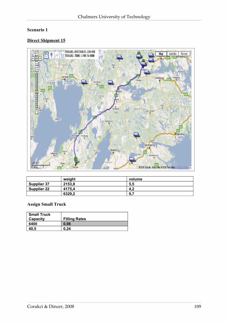
Chalmers University of Technology
Scenario 1
Direct Shipment 15
weight volumeSupplier 37 2153,8 5,5Supplier 22 4175,4 4,2 6329,2 9,7
Assign Small Truck
Small Truck Capacity Filling Rates6400 0,9840,5 0,24
Corakci & Dincer, 2008 109

Chalmers University of Technology
Scenario 1
Direct Shipment 16
weight volumeSupplier 23 1783,3 4,4Supplier 48 1136,4 4,7Supplier 42 2719,2 7 5638,9 16,1
Assign Small Truck
Small Truck Capacity Filling Rates6400 0,8840,5 0,40
Corakci & Dincer, 2008 110

Chalmers University of Technology
Scenario 1
Direct Shipment 17
weight volumeSupplier 11 359,2 1,8Supplier 26 34,5 0,1Supplier 36 517 3 910,8 4,9
Assign Cargo Van
Cargo Van Capacity Filling Rates1500 0,6015 0,33
Corakci & Dincer, 2008 111
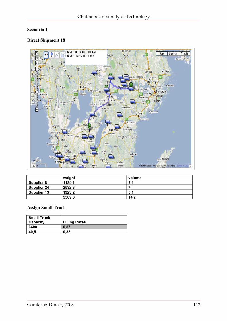
Chalmers University of Technology
Scenario 1
Direct Shipment 18
weight volumeSupplier 8 1134,1 2,1Supplier 24 2532,3 7Supplier 13 1923,2 5,1 5589,6 14,2
Assign Small Truck
Small Truck Capacity Filling Rates6400 0,8740,5 0,35
Corakci & Dincer, 2008 112
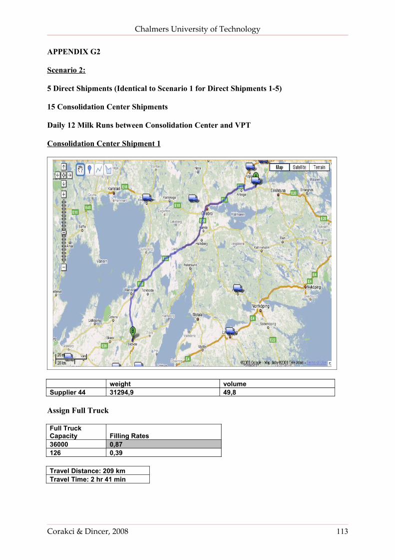
Chalmers University of Technology
APPENDIX G2
Scenario 2:
5 Direct Shipments (Identical to Scenario 1 for Direct Shipments 1-5)
15 Consolidation Center Shipments
Daily 12 Milk Runs between Consolidation Center and VPT
Consolidation Center Shipment 1
weight volumeSupplier 44 31294,9 49,8
Assign Full Truck
Full Truck Capacity Filling Rates36000 0,87126 0,39
Travel Distance: 209 kmTravel Time: 2 hr 41 min
Corakci & Dincer, 2008 113
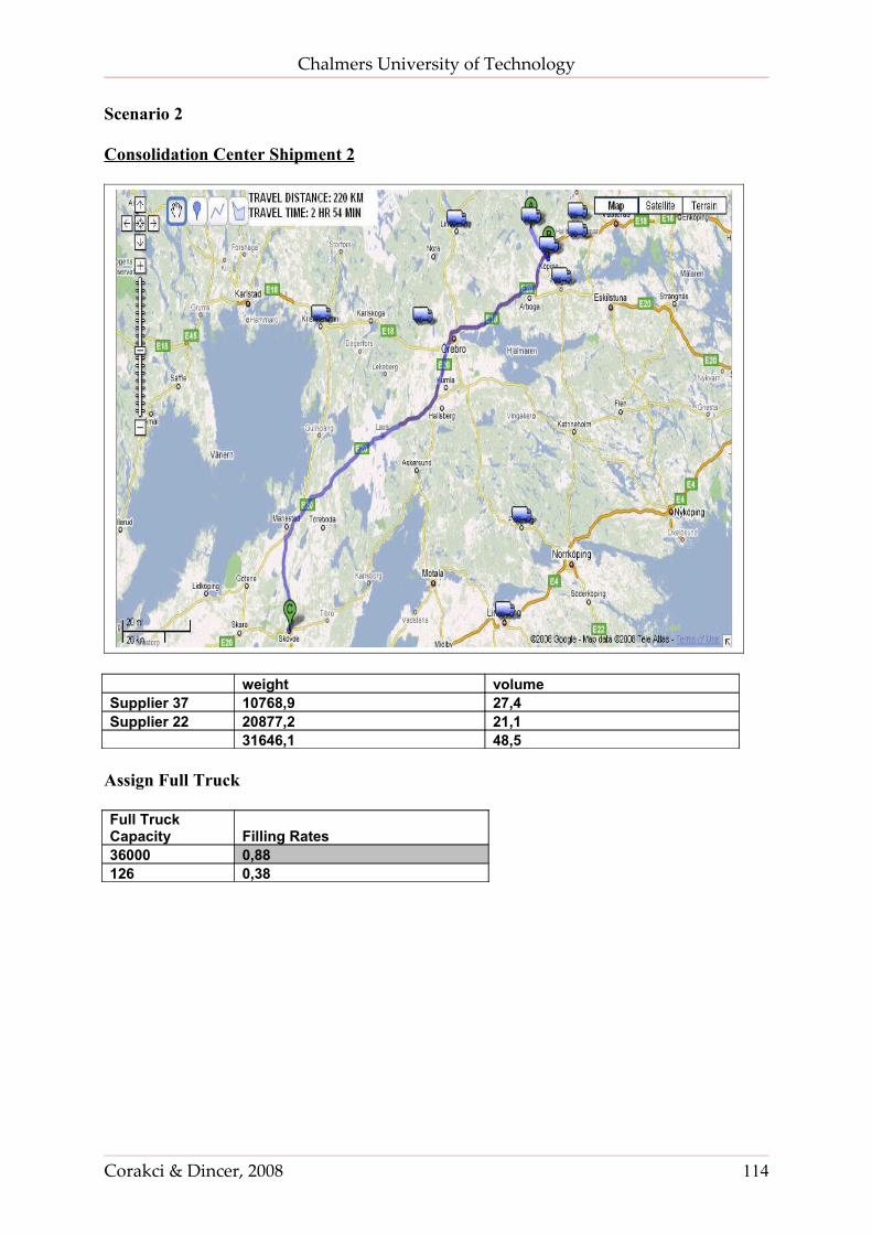
Chalmers University of Technology
Scenario 2
Consolidation Center Shipment 2
weight volumeSupplier 37 10768,9 27,4Supplier 22 20877,2 21,1 31646,1 48,5
Assign Full Truck
Full Truck Capacity Filling Rates36000 0,88126 0,38
Corakci & Dincer, 2008 114
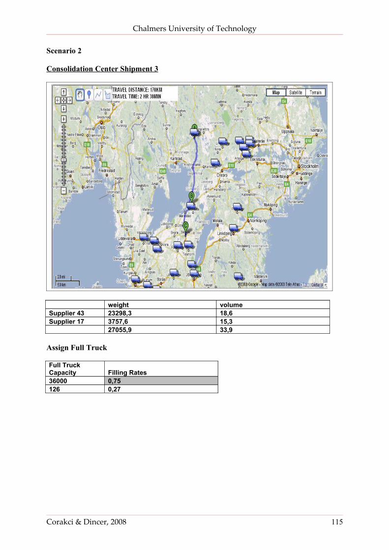
Chalmers University of Technology
Scenario 2
Consolidation Center Shipment 3
weight volumeSupplier 43 23298,3 18,6Supplier 17 3757,6 15,3 27055,9 33,9
Assign Full Truck
Full Truck Capacity Filling Rates36000 0,75126 0,27
Corakci & Dincer, 2008 115
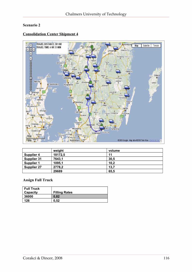
Chalmers University of Technology
Scenario 2
Consolidation Center Shipment 4
weight volumeSupplier 4 18172,5 11Supplier 31 7643,1 30,5Supplier 1 1095,1 10,2Supplier 27 2778,2 13,7 29689 65,5
Assign Full Truck
Full Truck Capacity Filling Rates36000 0,82126 0,52
Corakci & Dincer, 2008 116
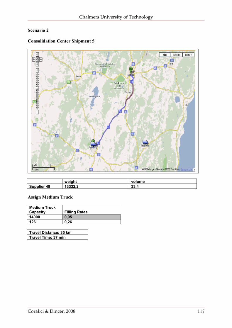
Chalmers University of Technology
Scenario 2
Consolidation Center Shipment 5
weight volumeSupplier 49 13332,2 33,4
Assign Medium Truck
Medium Truck Capacity Filling Rates14000 0,95126 0,26
Travel Distance: 35 kmTravel Time: 37 min
Corakci & Dincer, 2008 117
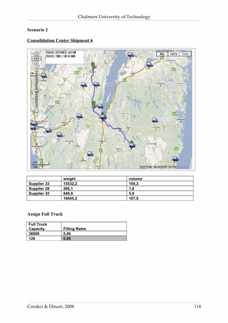
Chalmers University of Technology
Scenario 2
Consolidation Center Shipment 6
weight volumeSupplier 33 15532,2 100,2Supplier 28 266,1 1,8Supplier 35 846,8 5,9 16645,2 107,9
Assign Full Truck
Full Truck Capacity Filling Rates36000 0,46126 0,85
Corakci & Dincer, 2008 118
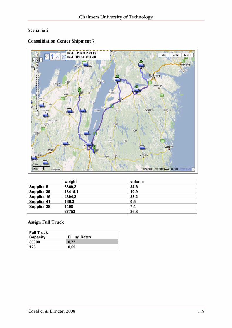
Chalmers University of Technology
Scenario 2
Consolidation Center Shipment 7
weight volumeSupplier 5 8369,2 34,6Supplier 39 13415,1 10,9Supplier 16 4394,3 33,2Supplier 41 166,3 0,5Supplier 38 1408 7,4 27753 86,8
Assign Full Truck
Full Truck Capacity Filling Rates36000 0,77126 0,69
Corakci & Dincer, 2008 119
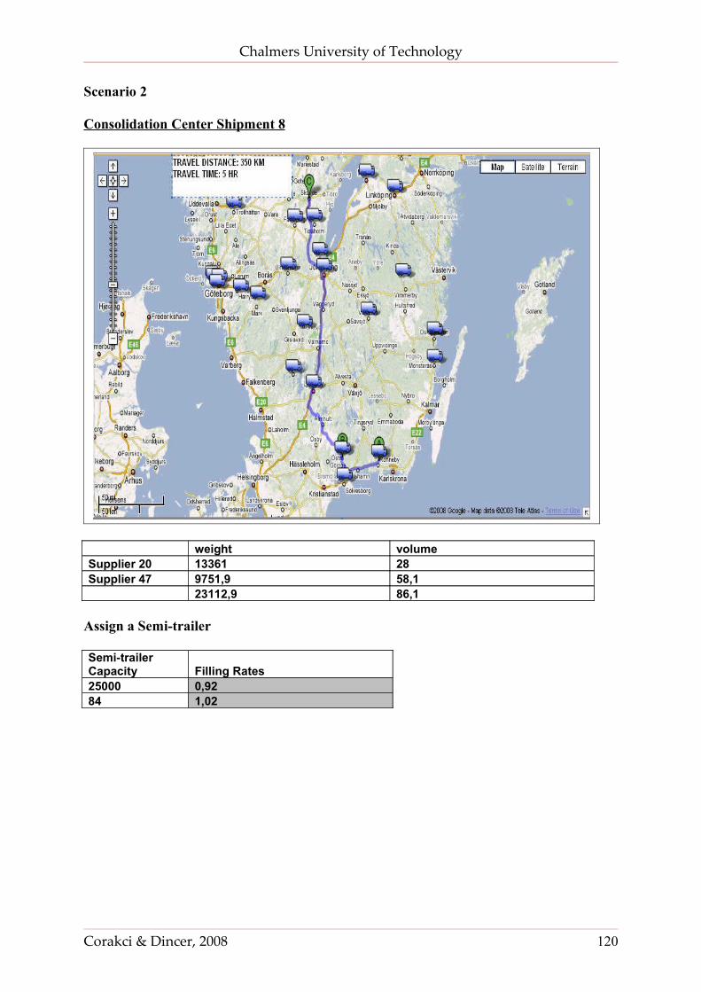
Chalmers University of Technology
Scenario 2
Consolidation Center Shipment 8
weight volumeSupplier 20 13361 28Supplier 47 9751,9 58,1 23112,9 86,1
Assign a Semi-trailer
Semi-trailer Capacity Filling Rates25000 0,9284 1,02
Corakci & Dincer, 2008 120
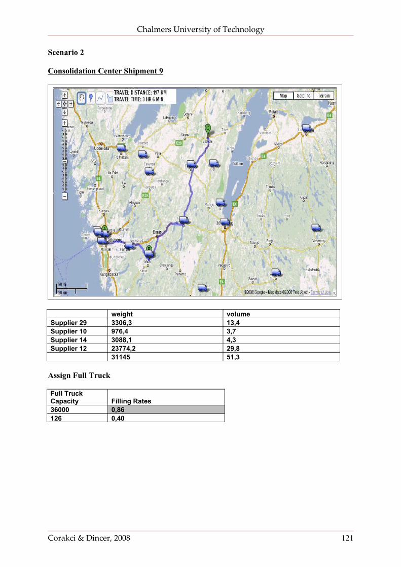
Chalmers University of Technology
Scenario 2
Consolidation Center Shipment 9
weight volumeSupplier 29 3306,3 13,4Supplier 10 976,4 3,7Supplier 14 3088,1 4,3Supplier 12 23774,2 29,8 31145 51,3
Assign Full Truck
Full Truck Capacity Filling Rates36000 0,86126 0,40
Corakci & Dincer, 2008 121
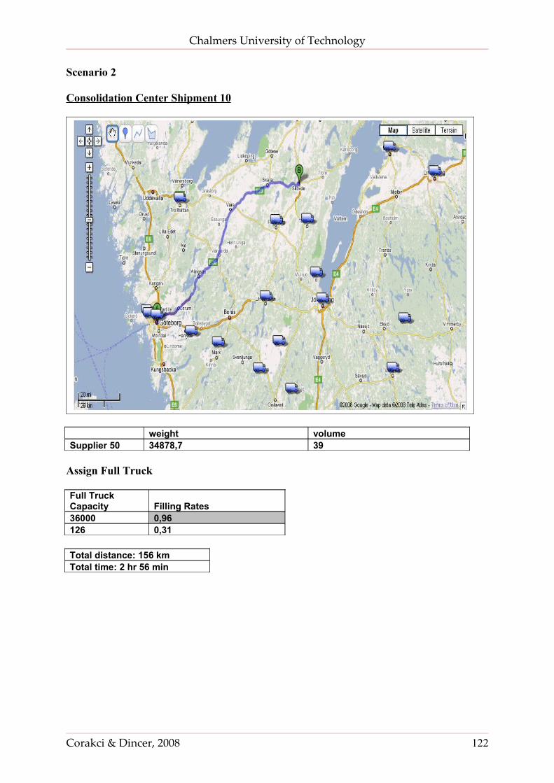
Chalmers University of Technology
Scenario 2
Consolidation Center Shipment 10
weight volumeSupplier 50 34878,7 39
Assign Full Truck
Full Truck Capacity Filling Rates36000 0,96126 0,31
Total distance: 156 kmTotal time: 2 hr 56 min
Corakci & Dincer, 2008 122
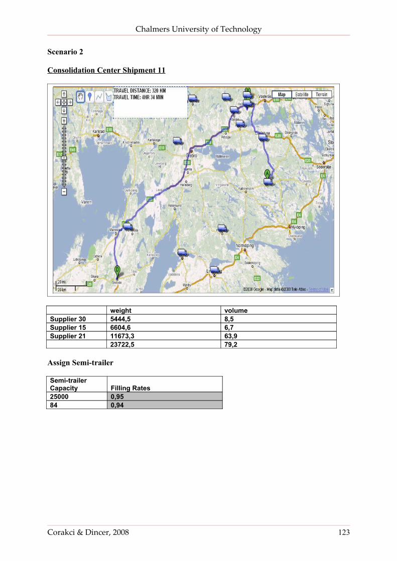
Chalmers University of Technology
Scenario 2
Consolidation Center Shipment 11
weight volumeSupplier 30 5444,5 8,5Supplier 15 6604,6 6,7Supplier 21 11673,3 63,9 23722,5 79,2
Assign Semi-trailer
Semi-trailer Capacity Filling Rates25000 0,9584 0,94
Corakci & Dincer, 2008 123
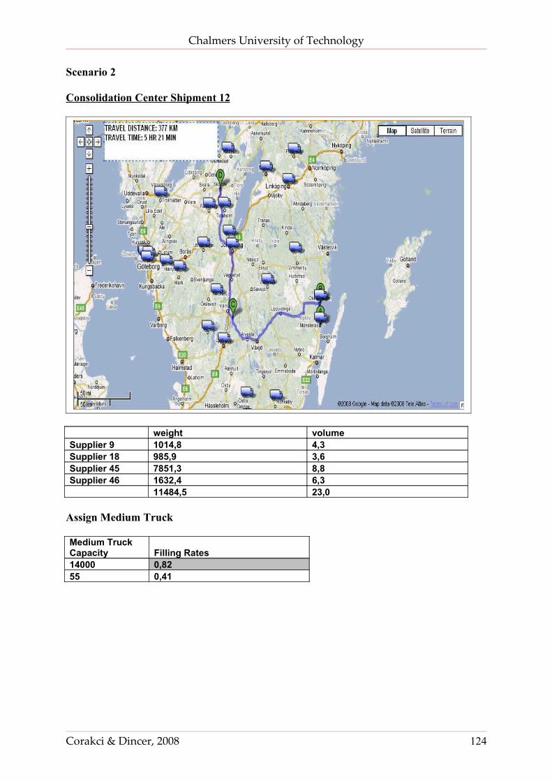
Chalmers University of Technology
Scenario 2
Consolidation Center Shipment 12
weight volumeSupplier 9 1014,8 4,3Supplier 18 985,9 3,6Supplier 45 7851,3 8,8Supplier 46 1632,4 6,3 11484,5 23,0
Assign Medium Truck
Medium Truck Capacity Filling Rates14000 0,8255 0,41
Corakci & Dincer, 2008 124
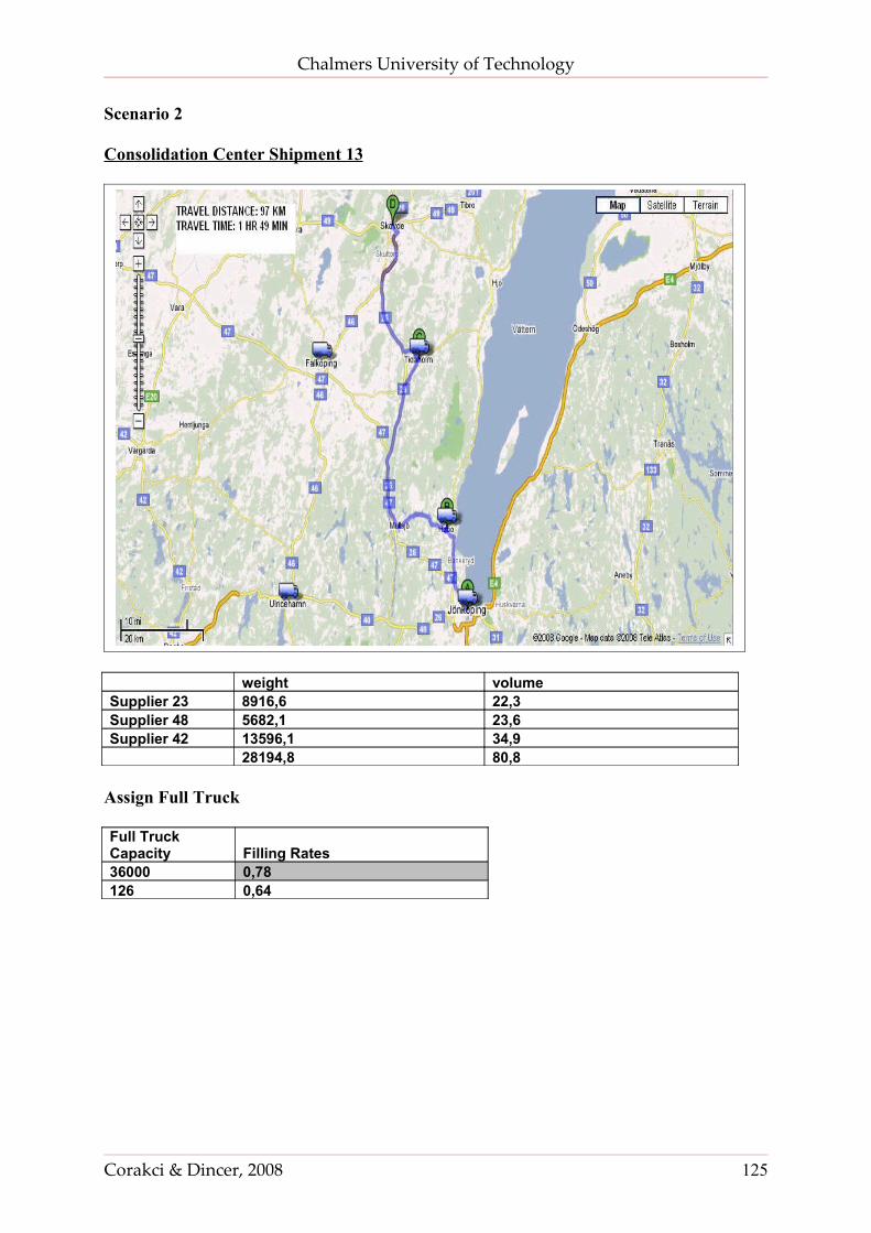
Chalmers University of Technology
Scenario 2
Consolidation Center Shipment 13
weight volumeSupplier 23 8916,6 22,3Supplier 48 5682,1 23,6Supplier 42 13596,1 34,9 28194,8 80,8
Assign Full Truck
Full Truck Capacity Filling Rates36000 0,78126 0,64
Corakci & Dincer, 2008 125
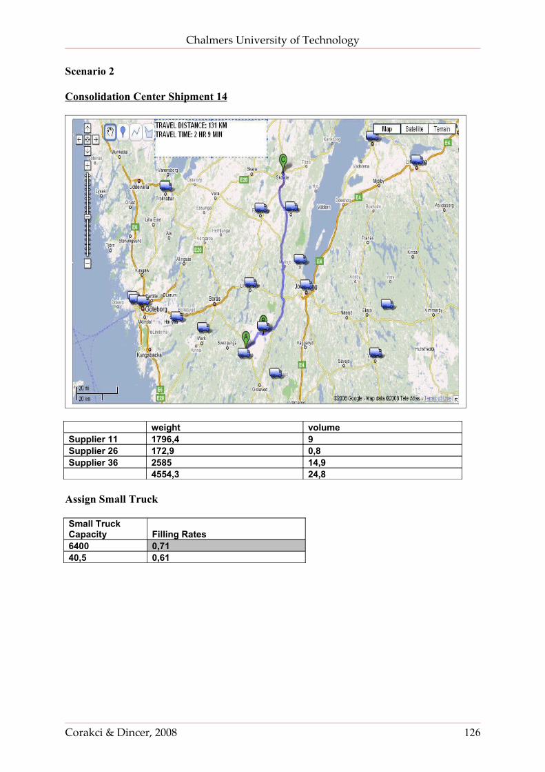
Chalmers University of Technology
Scenario 2
Consolidation Center Shipment 14
weight volumeSupplier 11 1796,4 9Supplier 26 172,9 0,8Supplier 36 2585 14,9 4554,3 24,8
Assign Small Truck
Small Truck Capacity Filling Rates6400 0,7140,5 0,61
Corakci & Dincer, 2008 126
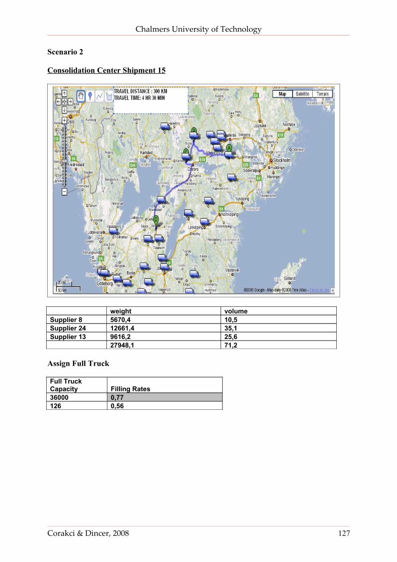
Chalmers University of Technology
Scenario 2
Consolidation Center Shipment 15
weight volumeSupplier 8 5670,4 10,5Supplier 24 12661,4 35,1Supplier 13 9616,2 25,6 27948,1 71,2
Assign Full Truck
Full Truck Capacity Filling Rates36000 0,77126 0,56
Corakci & Dincer, 2008 127
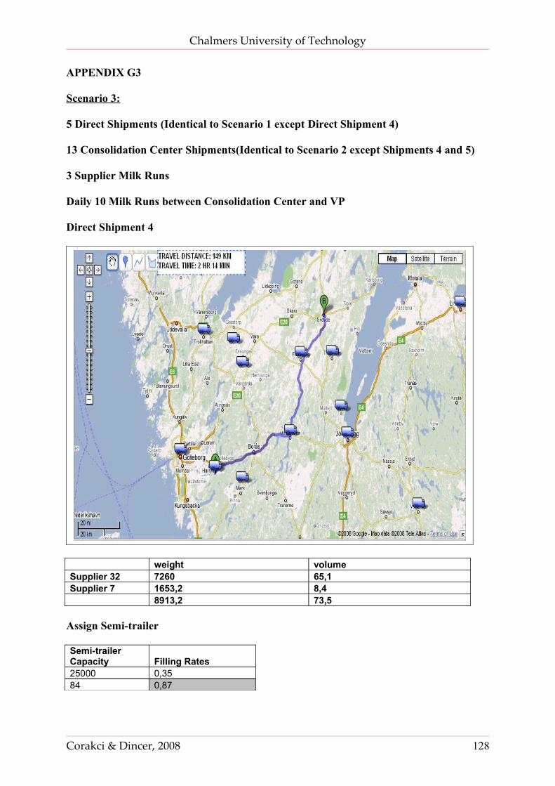
Chalmers University of Technology
APPENDIX G3
Scenario 3:
5 Direct Shipments (Identical to Scenario 1 except Direct Shipment 4)
13 Consolidation Center Shipments(Identical to Scenario 2 except Shipments 4 and 5)
3 Supplier Milk Runs
Daily 10 Milk Runs between Consolidation Center and VP
Direct Shipment 4
weight volumeSupplier 32 7260 65,1Supplier 7 1653,2 8,4 8913,2 73,5
Assign Semi-trailer
Semi-trailer Capacity Filling Rates25000 0,3584 0,87
Corakci & Dincer, 2008 128

Chalmers University of Technology
Scenario 3
Consolidation Center Shipment 4
weight volumeSupplier 4 18172,5 11,1Supplier 31 7643,2 30,6Supplier 1 1095,1 10,2 26910,8 51,9
Assign Full Truck
Full Truck Capacity Filling Rates36000 0,74126 0,41
Corakci & Dincer, 2008 129
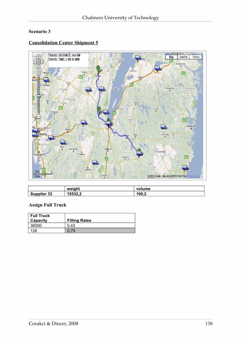
Chalmers University of Technology
Scenario 3
Consolidation Center Shipment 5
weight volumeSupplier 33 15532,2 100,2
Assign Full Truck
Full Truck Capacity Filling Rates36000 0,43126 0,79
Corakci & Dincer, 2008 130
Related Documents