PIPE STRESS ANALYSIS USING A COMPUTER MODEL OF THE PIPING SYSTEM

75577376 Point Pipe Stress Analysis by Computer CAESAR II
Nov 03, 2014
Welcome message from author
This document is posted to help you gain knowledge. Please leave a comment to let me know what you think about it! Share it to your friends and learn new things together.
Transcript
PIPE STRESS ANALYSIS USING A
COMPUTER MODEL OF THE PIPING SYSTEM
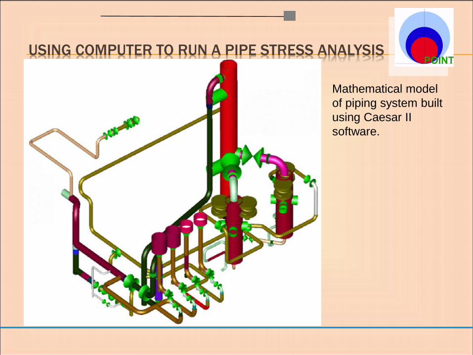
USING COMPUTER TO RUN A PIPE STRESS ANALYSIS
Mathematical model
of piping system built
using Caesar II
software.
BUILDING A MODEL WITH CAESAR II
Engineers nowadays do not have to worry about solving higher degree, or differential equations to perform complicated calculations, because they can create complete models of the system they are trying to design and analyse and let the software perform the analysis for them. However as the saying goes, “garbage in; garbage out” the engineer still has to possess good engineering judgment to know what to expect from a computer analysis and how to interpret the output.
Although there are various softwares available to do pipe stress analyses, Caesar II is one that is well known and frequently used for the oil and gas engineering analyses.

USING CAESAR II FOR PIPE ANALYSIS CAESAR II is most often used for the mechanical design of new piping systems.
Hot piping systems present a unique problem to the mechanical engineer—these
irregular structures experience great thermal strain that must be absorbed by the
piping, supports, and attached equipment. These “structures” must be stiff enough to
support their own weight and also flexible enough to accept thermal growth. These
loads, displacements, and stresses can be estimated through analysis of the piping
model in CAESAR II. To aid in this design by analysis, CAESAR II incorporates
many of the limitations placed on these systems and their attached equipment.
These limits are typically specified by engineering bodies (such as the ASME B31
committees, ASME Section VIII, and the Welding Research Council) or by
manufacturers of piping-related equipment (API, NEMA, or Expansion Joint
Manufacturers‟ Association - EJMA).
CAESAR II is not limited to thermal analysis of piping systems. CAESAR II also
has the capability of modeling and analyzing the full range of static and dynamic loads,
which may be imposed on the system. Therefore, CAESAR II is not only a tool for
new design but it is also valuable in troubleshooting or re-designing existing systems.
Here, one can determine the cause of failure or evaluate the severity of un-anticipated
operating conditions such as fluid/piping interaction or mechanical vibration caused by
rotating equipment.
CONFIGURING CAESAR II
Each time CAESAR II starts, the configuration file caesar.cfg is read from
the current data directory. If this file is not found in the current data directory,
eventually a fatal error will be generated and CAESAR II will terminate.
To generate the caesar.cfg file select Tools/Configure/Setup (or the
Configure button from the toolbar) from the CAESAR II Main Menu.
Once finished users must click Exit w/Save at the bottom of the
Configure/Setup window to create a new configuration file or to save
changes to the existing configuration file. The configuration program
produces the Computation Control window.
Important: The caesar.cfg file may vary from machine to machine and many of
the setup directives modify the analysis. The units' file, if modified by the user,
would also need to be identical if the same results are to be produced.
See the next slide for an image of the Computational Control panel.
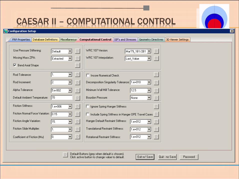
CAESAR II – COMPUTATIONAL CONTROL
CA
ES
AR
II
– C
OM
PU
TATIO
NA
L
CO
NTR
OL C
ON
FIG
UR
ATIO
N S
ETTIN
GS
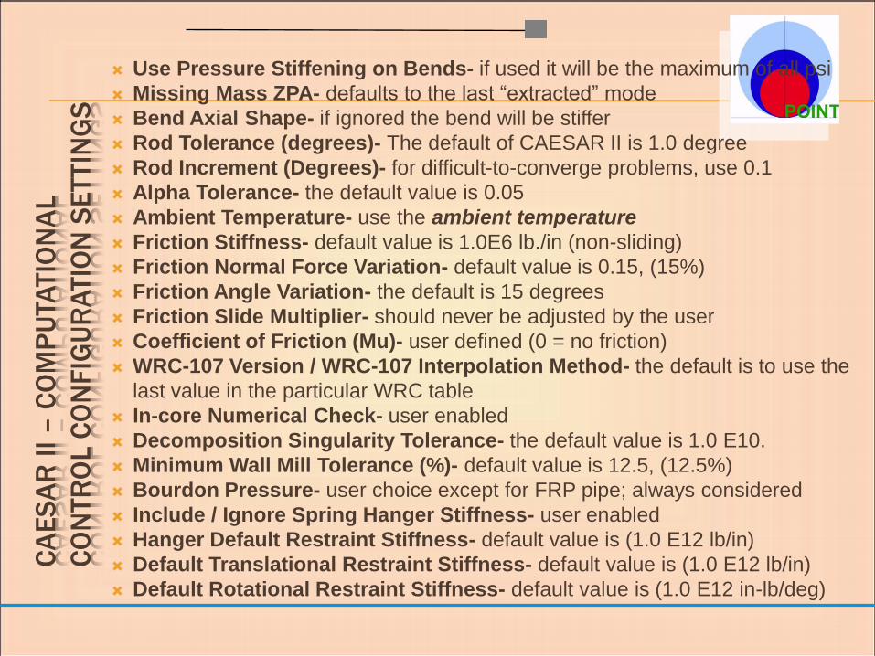
Use Pressure Stiffening on Bends- if used it will be the maximum of all psi
Missing Mass ZPA- defaults to the last “extracted” mode
Bend Axial Shape- if ignored the bend will be stiffer
Rod Tolerance (degrees)- The default of CAESAR II is 1.0 degree
Rod Increment (Degrees)- for difficult-to-converge problems, use 0.1
Alpha Tolerance- the default value is 0.05
Ambient Temperature- use the ambient temperature
Friction Stiffness- default value is 1.0E6 lb./in (non-sliding)
Friction Normal Force Variation- default value is 0.15, (15%)
Friction Angle Variation- the default is 15 degrees
Friction Slide Multiplier- should never be adjusted by the user
Coefficient of Friction (Mu)- user defined (0 = no friction)
WRC-107 Version / WRC-107 Interpolation Method- the default is to use the
last value in the particular WRC table
In-core Numerical Check- user enabled
Decomposition Singularity Tolerance- the default value is 1.0 E10.
Minimum Wall Mill Tolerance (%)- default value is 12.5, (12.5%)
Bourdon Pressure- user choice except for FRP pipe; always considered
Include / Ignore Spring Hanger Stiffness- user enabled
Hanger Default Restraint Stiffness- default value is (1.0 E12 lb/in)
Default Translational Restraint Stiffness- default value is (1.0 E12 lb/in)
Default Rotational Restraint Stiffness- default value is (1.0 E12 in-lb/deg)

CAESAR II – STRESS INTENSIFICATION FACTORS
(SIFS)
CA
ES
AR
II
– S
IFS
AN
D S
TR
ES
S
CO
NF
IGU
RA
TIO
N S
ETTIN
GS
Default Code
The piping code the user designs to most often should go here. This code
will be used as the default if no code is specified in the problem input. The
default piping code is B31.3, the chemical plant and petroleum refinery
code. Valid entries are B31.1, B31.3, B31.4, B31.4 Chapter IX, B31.5,
B31.8, B31.8 Chapter VIII, B31.11, ASME-NC(Class 2), ASME-ND(Class
3), NAVY505, Z662, Z662 Chapter 11, BS806, SWEDISH1, SWEDISH2,
B31.1-1967, STOOMWEZEN, RCCM-C, RCCM-D, CODETI, Norwegian,
FDBR, BS-7159, UKOOA, IGE/TD/12, DNV, EN-13480, and GPTC/192.
Occasional Load Factor
B31.3 states, “The sum of the longitudinal stresses due to pressure,
weight, and other sustained loadings (S1) and of the stresses produced by
occasional loads such as wind or earthquake may be as much as 1.33
times the allowable stress given in Appendix A…” The default for B31.3
applications is 33%. If this is too high for the material and temperature
specified then a smaller occasional load factor could be input.
Yield Stress Criterion:
Von Mises Theory or the
Maximum Shear Theory

CA
ES
AR
II
– C
OM
PU
TATIO
NA
L
CO
NTR
OL C
ON
FIG
UR
ATIO
N S
ETTIN
GS
(CO
NT’D
.)
B31.3 Sustained SIF Multiplier - the default is 1.0
B31.3 Welding and Contour Tees Meet B16.9- the default setting for this
directive is “NO”, which causes the program to use a flexibility characteristic
of 3.1*T/r, as per the A01 addendum.
Allow User's SIF at Bend- the default is off
Use WRC 329- this activates the WRC329 guidelines for all intersections
Use Schneider- activates the Schneider reduced intersection assumptions
All Cases Corroded- if enabled, uses the corroded section modulus
Liberal Expansion Stress Allowable- user choice to make it default
Press. Variation in Expansion Case- user controlled
Base Hoop Stress On ( ID/OD/Mean/Lamés )- The default is to use the ID
of the pipe. If enabled, hoop stress value has the following options:
ID—Hoop stress is computed according to Pd/2t where “d” is the internal
diameter of the pipe.
OD—Hoop stress is computed according to Pd/2t where “d” is the outer
diameter of the pipe.
Mean—Hoop stress is computed according to Pd/2t where “d” is the average
or mean diameter of the pipe.
Lamés—Hoop stress is computed according to Lamés equation, = P ( Ri2 +
Ri2 * Ro2 / R2 ) / ( Ro2 - Ri2 ) and varies through the wall as a function of R
CA
ES
AR
II
– C
OM
PU
TATIO
NA
L
CO
NTR
OL C
ON
FIG
UR
ATIO
N S
ETTIN
GS
(CO
NT’D
.)
Use PD/4t- The more comprehensive calculation, i.e. the Default, is
recommended
Add F/A in Stresses- setting this to „Default‟ causes CAESAR II to use
whatever the currently active piping code recommends.
Add Torsion in SL Stress- setting to „Yes‟ will include the torsion term in
those codes that don‟t include it already by default
Reduced Intersection- options are B31.1(Pre 1980), B31.1(Post 1980),
WRC329, ASME SEC III, and Schneider
Class 1 Branch Flexibility- Activates the Class 1 flexibility calculations
B31.1 Reduced Z Fix- if used in conjunction with B31.1, it makes the
correction to the reduced branch stress calculation that existed in the 1980
through 1989 versions of B31.1
No RFT/WLT in Reduced Fitting SIFs- If enabled will use distinct in-plane
and out-of-plane SIFs
Implement B31.3 Appendix P- implements the alternate rules in B31.3
Appendix P.

IMP
OR
TAN
T T
OP
ICS
IN
MO
DE
L
BU
ILD
ING
Bends:
Stiffened Bends
90-degree
Bends
Mitered Bends
Elbows
Expansion Joints Simple Bellows with
Pressure Thrust
Tied Bellows
Universal Joints
Hinged Joints
Slip Joints
Gimbal Joints
Ball Joints
Restraints: Anchors
Guides
Limit Stops
Windows
Double-Acting
Restraints
Hangers:
Single Can
Liftoff Spring Can
Bottom-out Spring Can
Constant Effort Hangers
Hanger w/ Sliding
Movement Capability Miscellaneous
Reducers
Jacketed Pipe
MODELLING PIPE BENDS
Bends are defined by the element entering the bend and the element
leaving the bend. The actual bend curvature is always physically at the “TO”
end of the element entering the bend.
(The element direction is defined from the first node to the second node.)
The input for the element leaving the bend must follow the element entering
the bend. The bend angle is defined by these two elements.
Bend radius defaults to 1 1/2 times the pipe nominal diameter (long radius),
but may be changed to any other value.
Specifying a bend automatically generates two additional intermediate
nodes, at the 0-degree location and at the bend midpoint (M).
For stress and displacement output the TO node of the element entering the
bend is located geometrically at the far-point on the bend. The far-point is at
the weld line of the bend, and adjacent to the straight element leaving the
bend.
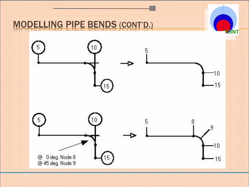
Nodes defined in the Angle and Node fields are placed at the given angle on
the bend curvature. The angle starts with zero degrees at the near-point on
the bend and goes to degrees at the far-point of the bend.
MODELLING PIPE BENDS (CONT’D.)
Nodes on the bend curvature cannot be placed closer together than
specified by the Minimum Angle to Adjacent Bend parameter in the
Configure-Setup—Geometry section. This includes the spacing
between the nodes on the bend curvature and the near and far-points of
the bend.
Entering the letter M as the angle designates the bend midpoints.
The minimum and maximum total bend angle is specified by the Minimum
Bend Angle and Maximum Bend Angle parameters in the Configure
Setup—Geometry section.
MODELLING PIPE BENDS (CONT’D.)
MODELLING PIPE SINGLE AND DOUBLE-FLANGED
BENDS Single and double flanged bend specifications only affect the stress
intensification and flexibility of the bend. There is no automatic rigid
element (or change in weight) generated for the end of the bend.
Single and double-flanged bends are indicated by entering 1 or 2
(respectively) for the Type in the bend auxiliary input.
Rigid elements defined before or after the bend will not alter the bend's
stiffness or stress intensification factors.
When specifying single flanged bends it does not matter which end of the
bend the flange is on.
If the user wishes to include the weight of the rigid flange(s) at the bend
ends, then he/she should put rigid elements (whose total length is the
length of a flange pair) at the bend ends where the flange pairs exist.
As a guideline, British Standard 806 recommends stiffening the bends
whenever a component that significantly stiffens the pipe cross section is
found within two diameters of either bend end.

MODELLING PIPE
SINGLE AND
DOUBLE-
FLANGED BENDS

MODELLING PIPE 180º RETURN BENDS
Two 90-degree bends
should be separated by
twice the bend radius.
The far-point of the first
bend is the same as the
near-point of the second
(following) the bend.
The user is recommended to put nodes at the
mid point of each bend comprising the 180
degree return. (See the example on this page)
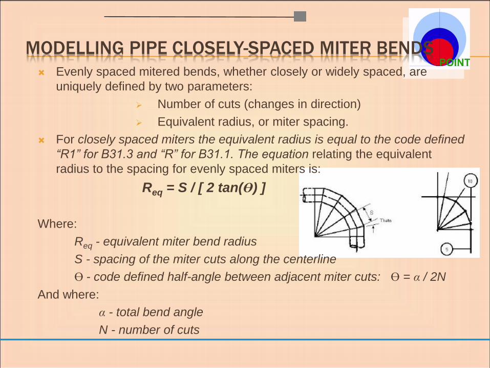
MODELLING PIPE CLOSELY-SPACED MITER BENDS
Evenly spaced mitered bends, whether closely or widely spaced, are
uniquely defined by two parameters:
Number of cuts (changes in direction)
Equivalent radius, or miter spacing.
For closely spaced miters the equivalent radius is equal to the code defined
“R1” for B31.3 and “R” for B31.1. The equation relating the equivalent
radius to the spacing for evenly spaced miters is:
Req = S / [ 2 tan(Ɵ) ]
Where:
Req - equivalent miter bend radius
S - spacing of the miter cuts along the centerline
Ɵ - code defined half-angle between adjacent miter cuts: Ɵ = α / 2N
And where:
α - total bend angle
N - number of cuts
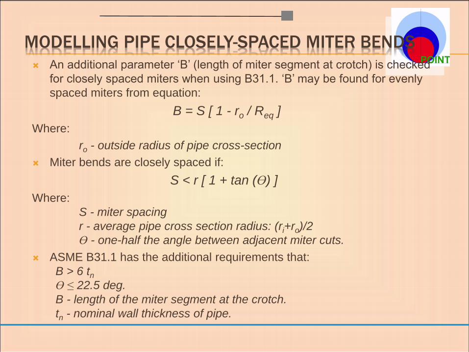
MODELLING PIPE CLOSELY-SPACED MITER BENDS
An additional parameter „B‟ (length of miter segment at crotch) is checked
for closely spaced miters when using B31.1. „B‟ may be found for evenly
spaced miters from equation:
B = S [ 1 - ro / Req ]
Where:
ro - outside radius of pipe cross-section
Miter bends are closely spaced if:
S < r [ 1 + tan (Ɵ) ]
Where:
S - miter spacing
r - average pipe cross section radius: (ri+ro)/2
Ɵ - one-half the angle between adjacent miter cuts.
ASME B31.1 has the additional requirements that:
B > 6 tn
Ɵ ≤ 22.5 deg.
B - length of the miter segment at the crotch.
tn - nominal wall thickness of pipe.
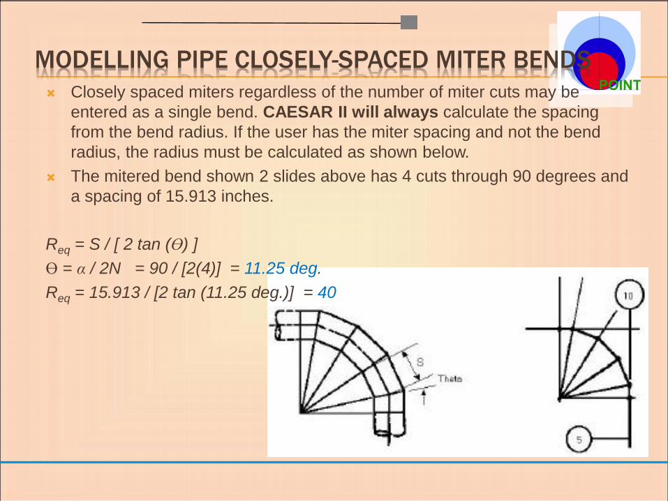
MODELLING PIPE CLOSELY-SPACED MITER BENDS
Closely spaced miters regardless of the number of miter cuts may be
entered as a single bend. CAESAR II will always calculate the spacing
from the bend radius. If the user has the miter spacing and not the bend
radius, the radius must be calculated as shown below.
The mitered bend shown 2 slides above has 4 cuts through 90 degrees and
a spacing of 15.913 inches.
Req = S / [ 2 tan (Ɵ) ]
Ɵ = α / 2N = 90 / [2(4)] = 11.25 deg.
Req = 15.913 / [2 tan (11.25 deg.)] = 40

MODELLING PIPE WIDELY-SPACED MITERED BENDS
Mitered bends are widely spaced if:
S ≥ r * [1 + tan (Ɵ)]
S - spacing between miter points along the miter segment centerline.
r - average cross section radius (ri+ro)/2
Ɵ - one-half angle between adjacent miter cuts.
B31.1 has the additional requirement that:
Ɵ ≤ 22.5 deg.
In CAESAR II, widely spaced miters must be entered as individual, single
cut miters, each having a bend radius equal to:
R = r [1 + cot (Ɵ)] / 2
R - reduced bend radius for widely spaced miters.
During error checking, CAESAR II will produce a warning message for
each mitered component, which does not pass the test for a closely
spaced miter. These components should be re-entered as a group of single
cut joints.
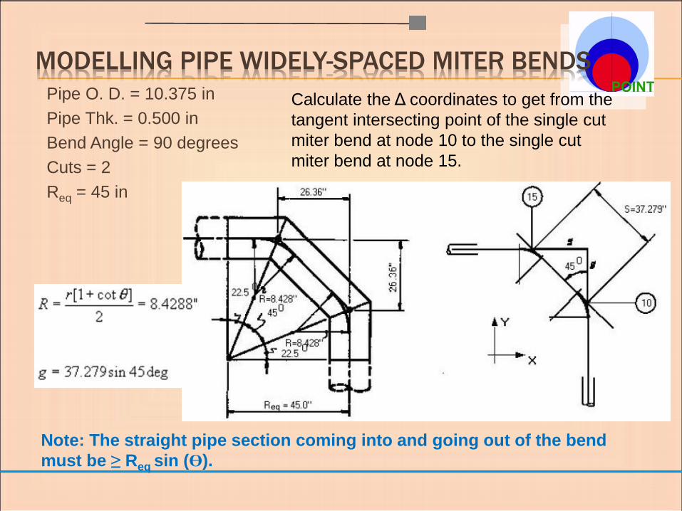
MODELLING PIPE WIDELY-SPACED MITER BENDS
Pipe O. D. = 10.375 in
Pipe Thk. = 0.500 in
Bend Angle = 90 degrees
Cuts = 2
Req = 45 in
Calculate the Δ coordinates to get from the
tangent intersecting point of the single cut
miter bend at node 10 to the single cut
miter bend at node 15.
Note: The straight pipe section coming into and going out of the bend
must be ≥ Req sin (Ɵ).
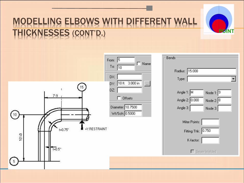
MODELLING ELBOWS WITH DIFFERENT WALL
THICKNESSES
When the fitting thickness in the bend auxiliary field is entered, CAESAR II
changes the thickness of the curved portion of the bend element only.
The thickness of any preceding or following straight pipe is unaffected.
The specified fitting thickness applies for the current elbow only and is not
carried on to any subsequent elbows in the job.
Stresses at the elbow are calculated based on the section modulus of the
matching pipe as specified in the B31 codes.
However, stress intensification factors and flexibility factors for the bend are
based on the elbow wall thickness.
The elbow at node 10 (in the next slide) has a thickness larger than the
matching pipe wall. The matching pipe has a thickness of 0.5
MODELLING ELBOWS WITH DIFFERENT WALL
THICKNESSES (CONT’D.)
RESTRAINTS
Anchors; Connecting nodes can be used with anchors to rigidly fix one
point in the piping system to any other point in the piping system.
Double-acting restraints; Double-acting restraints are those that act in
both directions along the line of action. Most commonly used restraints are
double-acting. A CNode is the connecting node.
Single-directional restraints; Friction and gaps may be specified with
single-directional restraints. A CNode is the connecting node.
Guides; Guides are double-acting restraints with or without a specified gap.
Connecting Nodes (CNodes) can be used with guides.
Limit Stop; Limit stops are single- or double-acting restraint whose line of
action is along the axis of the pipe. These can have gaps too. A gap is a
length, and is always positive.
Windows; Equal leg windows are modeled using two double-acting
restraints with gaps orthogonal to the pipe axis. Unequal leg windows are
modeled using four single-acting restraints with gaps orthogonal to the pipe
axis.
RESTRAINTS (CONT’D.)
Vertical / Horizontal Dummy Legs; Dummy legs and/or any other elements
attached to the bend curvature should be coded to the bend tangent
intersection point. For each dummy leg/bend model a warning message is
generated during error checking in CAESAR II.
Large Rotation rods; Large rotation rods are used to model relatively short
rods, where large orthogonal movement of the pipe causes shortening of the
restraint along the original line of action. These can be entered in any
direction. Large rotation is generally considered to become significant when
the angle of swing becomes greater than 5 degrees.
Static Snubbers; Translational restraints that provide resistance to
displacement in static analysis of occasional loads only. Static snubbers may
be directional, (i.e. may be preceded by a plus or minus sign).
Plastic Hinges; Two bi-linear supports are used to model rigid resistance to
bending until a breakaway force (yield force) is exceeded at which point
bending is essentially free.
Sway Brace assemblies; The sway brace is composed of a single
compression spring enclosed between two movable plates. Manufacturers
typically recommend a specific size sway brace for a given pipe nominal
diameter.

SPRING HANGERS
The hanger design algorithm will not design hangers that are completely
predefined. Any other data can exist for the spring location but this data
is not used. Entered spring rates and theoretical cold loads will be
multiplied by the number of hangers at this location. CAESAR II
requires the Theoretical Cold (Installation) Load to pre-define the
spring.
Theoretical Cold Load = Hot Load + Travel * Spring Rate
where upward travel is positive.
The basic parameters input into CAESAR II describe the wave height and
period, and the current velocity. The most difficult to obtain, and also the most
important parameters, are:
the drag, Cd
inertia, Cm and
lift coefficients, Cl
Based on the recommendations of API RP2A and DNV (Det Norske Veritas),
values for Cd range from 0.6 to 1.2, values for Cm range from 1.5 to 2.0. Values
for Cl show a wide range of scatter, but the approximate mean value is 0.7. The
inertia coefficient Cm is equal to one plus the added mass coefficient Ca. This
added mass value accounts for the mass of the fluid assumed to be entrained
with the piping element.
In actuality, these coefficients are a function of the fluid particle velocity, which
varies over the water column. In general practice, two dimensionless
parameters are computed which are used to obtain the Cd, Cm, and Cl values
from published charts.
NOTES ON CAESAR II HYDRODYNAMIC LOADING
This is a critical item for leakage determination and for computing
stresses in the flange.
The ASME code bases its stress calculations on a pre-specified, fixed equation
for the bolt stress. The resulting value is however often not related to the actual
tightening stress that appears in the flange when the bolts are tightened. For
this reason, the initial bolt stress input field that appears in the first section of
data input, Bolt Initial Tightening Stress, is used only for the flexibility/leakage
determination. The value for the bolt tightening stress used in the ASME flange
stress calculations is as defined by the ASME code:
Bolt Load = Hydrostatic End Force + Force for Leak-tight Joint
If the Bolt Initial Tightening Stress field is left blank, CAESAR II uses the value:
45000 / √(dbolt)
where 45,000 psi is a constant and d is the nominal diameter of the bolt
(correction is made for metric units).
NOTES ON BOLT TIGHTENING STRESS
This is a rule of thumb tightening stress, that will typically be applied by field
personnel tightening the bolts. This computed value is printed in the output from
the flange program.
It is interesting to compare this value to the bolt stress printed in the ASME
stress report (also in the output). It is not unusual for the “rule-of-thumb”
tightening stress to be larger than the ASME required stress. When the ASME
required stress is entered into the Bolt Initial Tightening Stress data field, a
comparison of the leakage safety factors can be made and the sensitivity of the
joint to the tightening torque can be ascertained. Users are strongly encouraged
to “play” with these numbers to get a feel for the relationship
between all of the factors involved.
NOTES ON BOLT TIGHTENING STRESS (CONT’D.)

MODELLING EXPANSION JOINTS
To define an expansion joint, activate the Expansion Joint check box (see
"Expansion Joints" on page 3-21 of the Caesar II manual) on the pipe
element spreadsheet.
The expansion joint will have a non-zero length if at least one of the
element‟s spreadsheet Delta fields is non-blank and non-zero. This will
usually result in a more accurate stiffness model in what is typically a very
sensitive area of the piping system.
Four stiffnesses define the expansion joint:
Axial Stiffness
Transverse Stiffness
Bending Stiffness
Torsional Stiffness
These stiffnesses are defined as shown in the figure shown in the next slide:
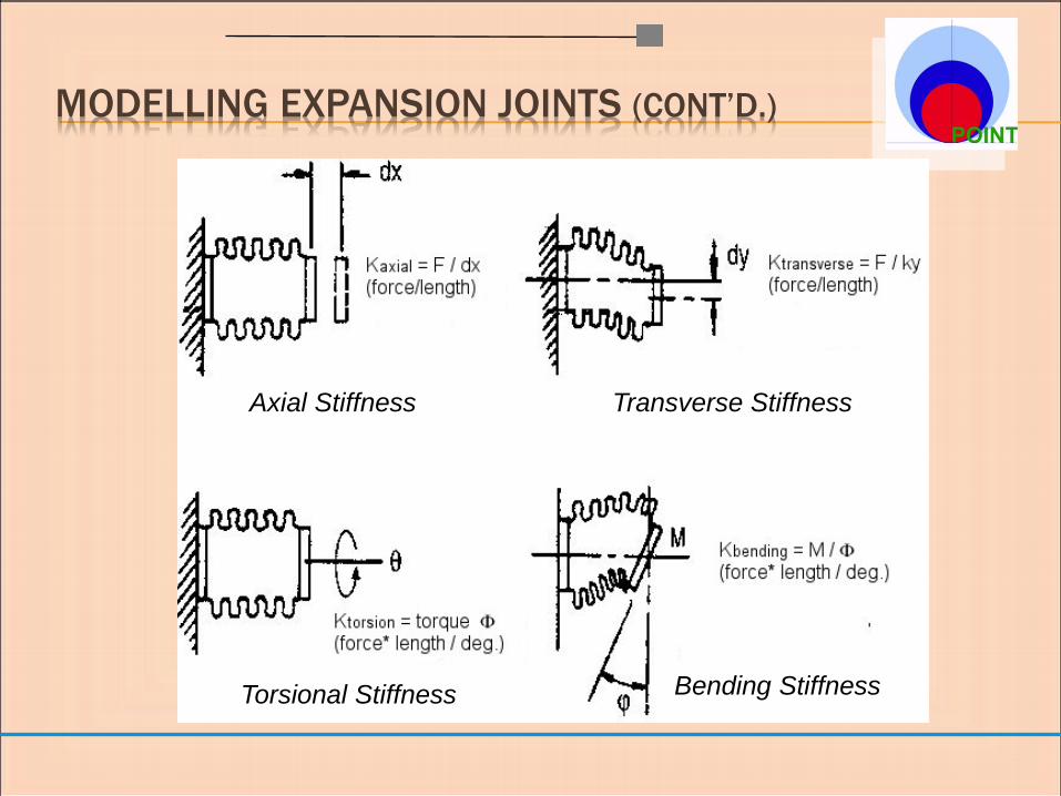
MODELLING EXPANSION JOINTS (CONT’D.)
Axial Stiffness Transverse Stiffness
Bending Stiffness Torsional Stiffness
MODELLING EXPANSION JOINTS (CONT’D.)
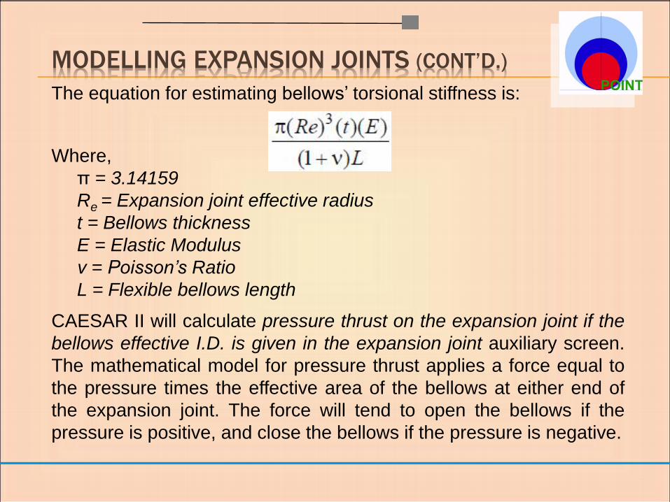
The equation for estimating bellows‟ torsional stiffness is:
Where,
π = 3.14159
Re = Expansion joint effective radius
t = Bellows thickness
E = Elastic Modulus
ν = Poisson’s Ratio
L = Flexible bellows length
CAESAR II will calculate pressure thrust on the expansion joint if the
bellows effective I.D. is given in the expansion joint auxiliary screen.
The mathematical model for pressure thrust applies a force equal to
the pressure times the effective area of the bellows at either end of
the expansion joint. The force will tend to open the bellows if the
pressure is positive, and close the bellows if the pressure is negative.
MODELLING EXPANSION JOINTS (CONT’D.)
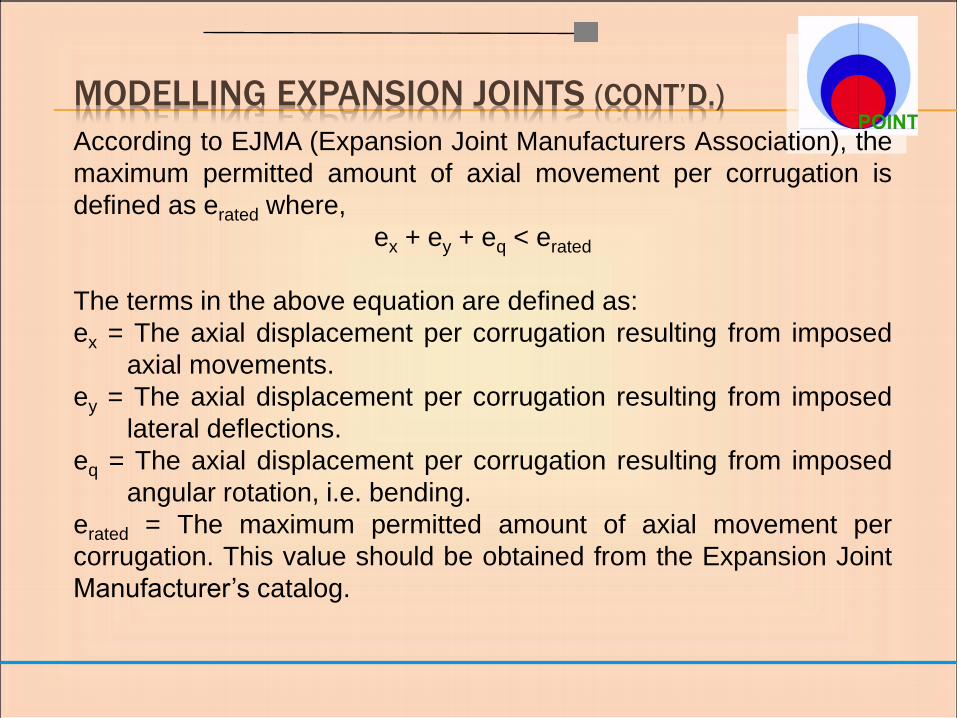
According to EJMA (Expansion Joint Manufacturers Association), the
maximum permitted amount of axial movement per corrugation is
defined as erated where,
ex + ey + eq < erated
The terms in the above equation are defined as:
ex = The axial displacement per corrugation resulting from imposed
axial movements.
ey = The axial displacement per corrugation resulting from imposed
lateral deflections.
eq = The axial displacement per corrugation resulting from imposed
angular rotation, i.e. bending.
erated = The maximum permitted amount of axial movement per
corrugation. This value should be obtained from the Expansion Joint
Manufacturer‟s catalog.
MODELLING EXPANSION JOINTS (CONT’D.)
The EJMA states:
“Also, [as an expansion joint is rotated or deflected laterally] it should
be noted that one side of the bellows attains a larger projected area
than the opposite side. Under the action of the applied pressure,
unbalanced forces are set up which tend to distort the expansion joint
further. In order to control the effects of these two factors a second
limit is established by the manufacturer upon the amount of angular
rotation and/or lateral deflection which may be imposed upon the
expansion joint. This limit may be less than the rated movement.
Therefore, in the selection of an expansion joint, care must be
exercised to avoid exceeding either of these manufacturer‟s limits.”
MODELLING EXPANSION JOINTS (CONT’D.)
CAESAR II computes the terms defined in the erated equation
and the movement of the joint ends relative to each other. These
relative movements are reported in both the local joint coordinate
system and the global coordinate system.
The expansion joint rating module can be entered by selecting Main
Menu Analysis - Expansion Joint Rating option.

MODELLING PIPE SPRINGS Spring Design Requirements
The smallest single spring that satisfies all design requirements is
selected as the designed spring.
The spring design requirements are:
Both the hot and the cold loads must be within the spring allowed working
range.
If the user specified an allowed load variation then the absolute value of the
product of the travel and the spring rate divided by the hot load must be
less than the specified variation.
If the user specified some minimum available clearance then the spring
selected must fit in this space.
If a single spring cannot be found that satisfies the design requirements,
CAESAR II will try to find two identical springs that do satisfy the
requirements.
If satisfactory springs cannot be found, CAESAR II recommends a
constant effort support for the location.
MODELLING PIPE SPRINGS (CONT’D.)
Setting Up the Spring Load Cases
The load cases that must exist for hanger design, as described above,
are:
Restrained Weight
Operating
Installed Weight ...if the user requested actual hanger installed loads.
After the hanger algorithm has run the load cases it needs to size the
hangers. The newly selected springs are inserted into the piping system
and included in the analysis of all remaining load cases.
The spring rate becomes part of the global stiffness matrix, and is
therefore added into all subsequent load cases.

MODELLING PIPE BRANCH FLEXIBILITIES
When the Class 1 branch flexibilities are used, intersection
models in the analysis will become stiffer when the reduced
geometry requirements do not apply, and will become more
flexible when the reduced geometry requirements do apply.
Stiffer intersections typically carry more load, and thus have
higher stresses (lowering the stress in other parts of the system
that have been “unloaded”).
More flexible intersections typically carry less load, and thus
have lower stresses, (causing higher stresses in other parts of
the system that have “picked up” the extra load).
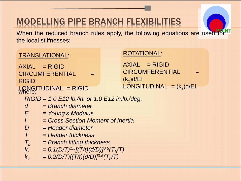
MODELLING PIPE BRANCH FLEXIBILITIES
When the reduced branch rules apply, the following equations are used for
the local stiffnesses:
TRANSLATIONAL:
AXIAL = RIGID
CIRCUMFERENTIAL =
RIGID
LONGITUDINAL = RIGID
ROTATIONAL:
AXIAL = RIGID
CIRCUMFERENTIAL =
(kx)d/EI
LONGITUDINAL = (kz)d/EI where:
RIGID = 1.0 E12 lb./in. or 1.0 E12 in.lb./deg.
d = Branch diameter
E = Young’s Modulus
I = Cross Section Moment of Inertia
D = Header diameter
T = Header thickness
Tb = Branch fitting thickness
kx = 0.1(D/T)1.5[(T/t)(d/D)]0.5(Tb/T)
kz = 0.2(D/T)[(T/t)(d/D)]0.5(Tb/T)
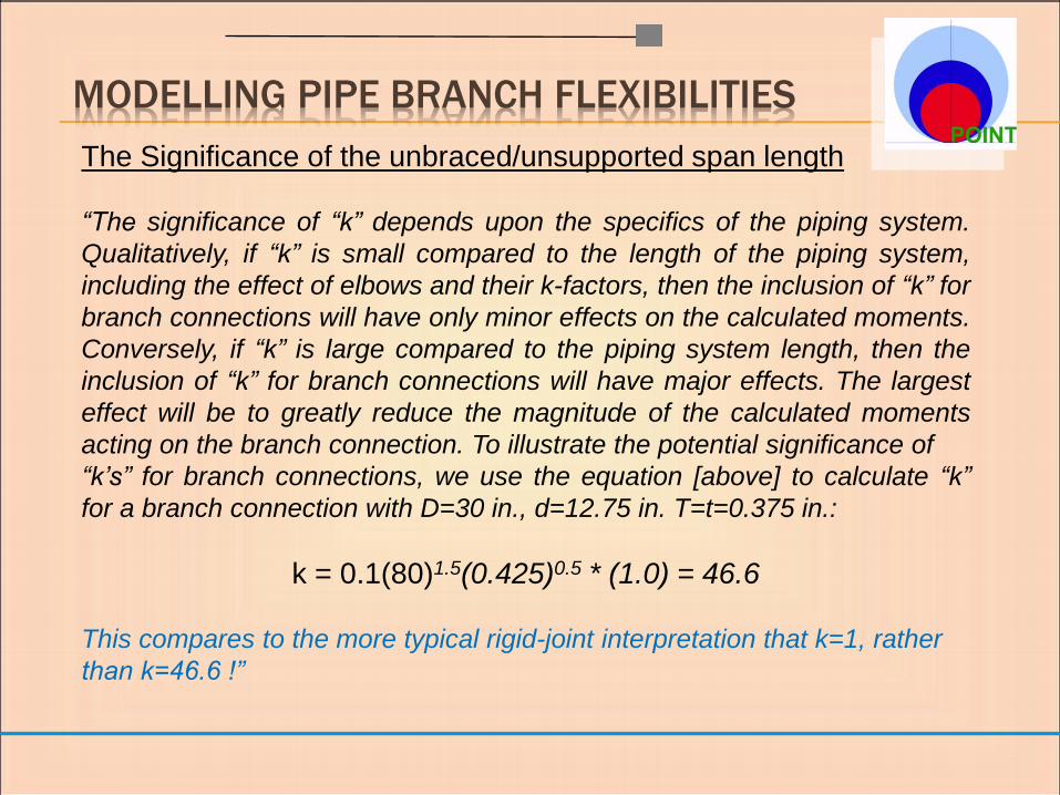
MODELLING PIPE BRANCH FLEXIBILITIES
The Significance of the unbraced/unsupported span length
“The significance of “k” depends upon the specifics of the piping system.
Qualitatively, if “k” is small compared to the length of the piping system,
including the effect of elbows and their k-factors, then the inclusion of “k” for
branch connections will have only minor effects on the calculated moments.
Conversely, if “k” is large compared to the piping system length, then the
inclusion of “k” for branch connections will have major effects. The largest
effect will be to greatly reduce the magnitude of the calculated moments
acting on the branch connection. To illustrate the potential significance of
“k’s” for branch connections, we use the equation [above] to calculate “k”
for a branch connection with D=30 in., d=12.75 in. T=t=0.375 in.:
k = 0.1(80)1.5(0.425)0.5 * (1.0) = 46.6
This compares to the more typical rigid-joint interpretation that k=1, rather
than k=46.6 !”
The following input parameters are required to get a leakage report. These
parameters include:
Flange Inside Diameter
Flange Thickness
Bolt Circle Diameter
Number Of Bolts
Bolt Diameter
Effective Gasket Diameter
Uncompressed Gasket Thickness
Effective Gasket Width
Leak Pressure Ratio
Effective Gasket Modulus
Externally Applied Moment
Externally Applied Force
Pressure
MODELLING PIPE FLANGES
Leak Pressure Ratio
This value is taken directly from Table 2-5.1 in the ASME Section VIII code.
This table is reproduced in the help screens of the software. This value is
more commonly recognized as “m”, and is termed the “Gasket Factor” in the
ASME code. This is a very important number for leakage determination, as it
represents the ratio of the pressure required to prevent leakage over the line
pressure.
Effective Gasket Modulus
Typical values are between 300,000 and 400,000 psi (20,684.27 and
27,579.03 bar) for spiral wound gaskets. The higher the modulus the greater
the tendency for the program to predict leakage. Errors on the high side
when estimating this value will lead to a more conservative design.
MODELLING PIPE FLANGES (CONT’D.)
Flange Rating This is an optional input, but results in some very interesting output. As mentioned
above, it has been a widely used practice in the industry to use the ANSI B16.5 and
API 605 temperature/pressure rating tables as a gauge for leakage. Because these
rating tables are based on allowable stresses, and were not intended for leakage
prediction, the leakage predictions that resulted were a function of the allowable
stress for the flange material, and not the flexibility, i.e. modulus of elasticity of the
flange. To give the user a “feel” for this old practice, the minimum and maximum
rating table values from ANSI and API were stored and are used to print minimum
and maximum leakage safety factors that would be predicted from this method.
Example output that the user will get upon entering the flange rating is shown as
follows:
EQUIVALENT PRESSURE MODEL ————————-
Equivalent Pressure (lb./sq.in.) 1639.85
ANSI/API Min Equivalent Pressure Allowed 1080.00
ANSI/API Max Equivalent Pressure Allowed 1815.00
This output shows that leakage, according to this older method, occurred if a carbon
steel flange was used, and leakage did not occur if an alloy flange was used. (Of
course both flanges would have essentially the same “flexibility” tendency to leak.)
MODELLING PIPE FLANGES (CONT’D.)
The B31G criteria provides a methodology whereby corroded pipelines can be
evaluated to determine when specific pipe segments must be replaced. The
original B31G document incorporates a healthy dose of conservatism and as a
result, additional work has been performed to modify the original criteria. This
additional work can be found in project report PR-3805, by Battelle, Inc. The
details of the original B31G criteria as well as the modified methods are
discussed in detail in this report.
CAESAR II determines the following values according to the original B31G
criteria and four modified methods.
These values are:
The hoop stress to cause failure
The maximum allowed operating pressure
The maximum allowed flaw length
MODELLING THE REMAINING STRENGTH OF CORRODED
PIPES

The four modified methods vary in the manner in which the corroded area is
estimated.
These methods are:
.85dL—The corroded area is approximated as 0.85 times the maximum pit
depth times the flaw length.
Exact—The corroded area is determined numerically using the trapezoid
method.
Equivalent—The corroded area is determined by multiplying the average pit
depth by the flaw length. Additionally, an equivalent flaw length (flaw length *
average pit depth / maximum pit depth) is used in the computation of the
Folias factor.
Effective—This method also uses a numerical trapezoid summation,
however, various sub lengths of the total flaw length are used to arrive at a
worst case condition.
Note that if the sub length which produces the worst case coincides with the
total length, the Exact and Effective methods yield the same result.
MODELLING THE REMAINING STRENGTH OF CORRODED
PIPES (CONT’D.)
ANALYSIS OPTIONS IN CAESAR II
• Statics—Performs Static analysis of pipe and/or structure. This is available
after error checking the input file.
• Dynamics—Performs Dynamic analysis of pipe and/or structure. This is also
available after error checking the input file.
• SIFs—Displays scratch pads used to calculate stress intensification factors at
intersections and bends.
• WRC 107/297—Calculates stresses in vessels due to attached piping.
• Flanges—Performs flange stress and leakage calculations.
• B31.G—Estimates pipeline remaining life.
• Expansion Joint Rating—Evaluates expansion joints using EJMA equations.
• AISC—Performs AISC code check on structural steel elements.
• NEMA SM23—Evaluates piping loads on steam turbine nozzles.
• API 610—Evaluates piping loads on centrifugal pumps.
• API 617—Evaluates piping loads on compressors.
• API 661—Evaluates piping loads on air-cooled heat exchangers.
• HEI Standard—Evaluates piping loads on feedwater heaters.
• API 560—Evaluates piping loads on fired heaters.
ERROR CHECKING IN CAESAR II
Static analysis cannot be performed until the error checking portion of the piping
pre-processor has been successfully completed. Only after error checking is
completed are the required analysis data files created. Similarly, any subsequent
changes made to the model input are not reflected in the analysis unless error
checking is rerun after those changes have been made. CAESAR II does not allow
an analysis to take place if the input has been changed and not successfully error
checked.
Error Checking can only be done from the input spreadsheet, and is
initiated by executing the Error Check or Batch Run commands from the
toolbar or menu. Error Check saves the input and starts the error checking
procedure.
Batch Run causes the program to check the input data, analyze the system,
and present the results without any user interaction. The assumptions
are that the loading cases to be analyzed do not need to change
Users may sort messages in the Message Grid by type, message number or
element/node number by double-clicking the corresponding column header.
Users can also print messages displayed in the Message Grid.
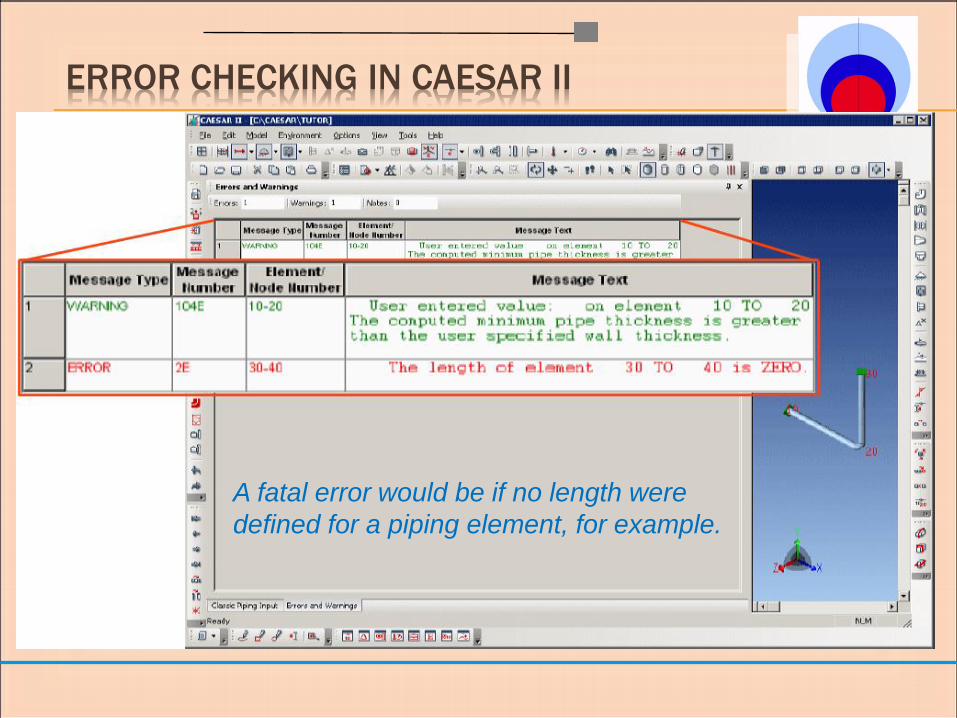
ERROR CHECKING IN CAESAR II
A fatal error would be if no length were
defined for a piping element, for example.
ERROR CHECKING IN CAESAR II (CONT’D.)
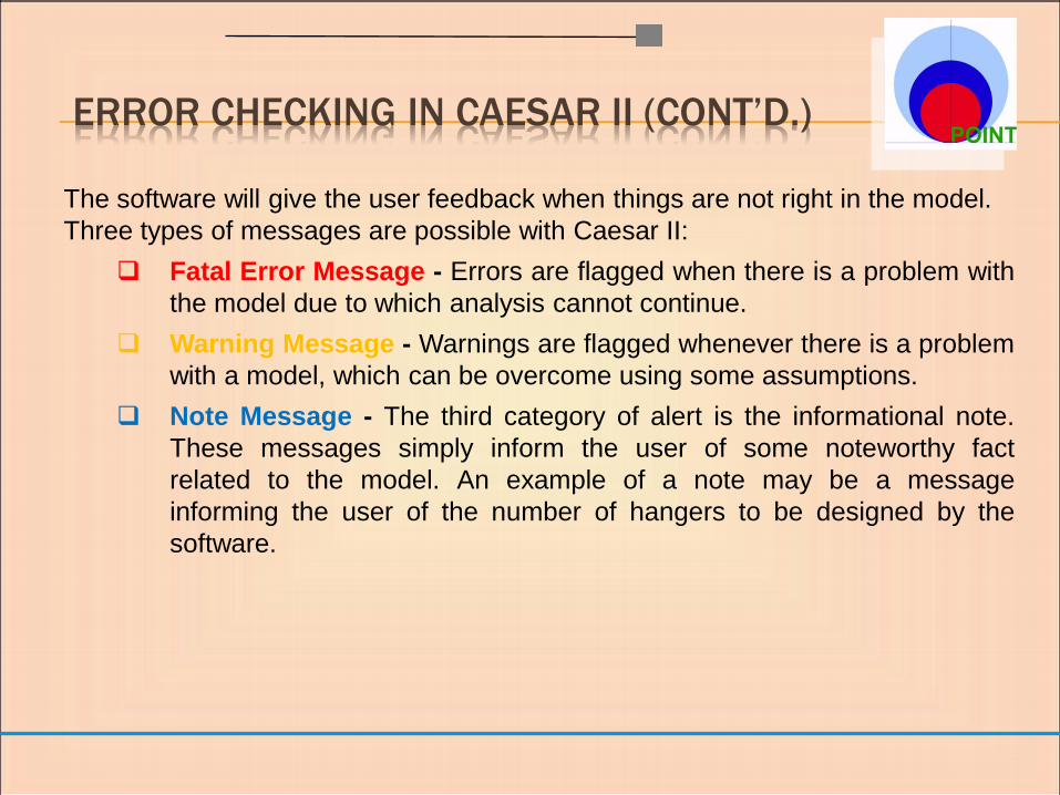
The software will give the user feedback when things are not right in the model.
Three types of messages are possible with Caesar II:
Fatal Error Message - Errors are flagged when there is a problem with
the model due to which analysis cannot continue.
Warning Message - Warnings are flagged whenever there is a problem
with a model, which can be overcome using some assumptions.
Note Message - The third category of alert is the informational note.
These messages simply inform the user of some noteworthy fact
related to the model. An example of a note may be a message
informing the user of the number of hangers to be designed by the
software.

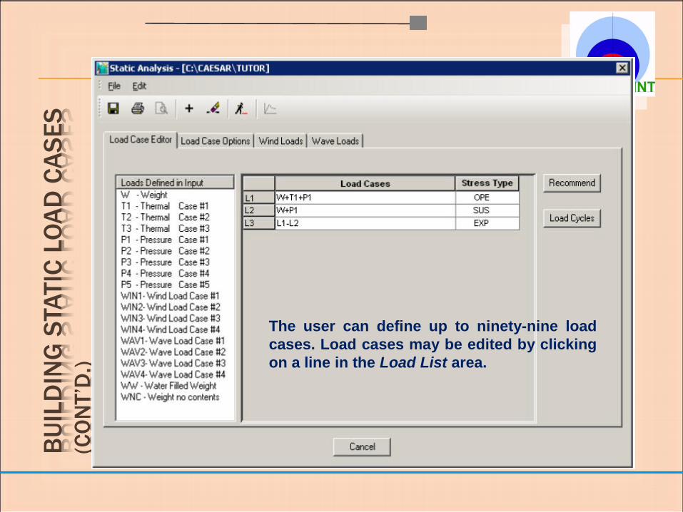
BUILDING STATIC LOAD CASES IN CAESAR II
The first step in the analysis of an error-checked piping model is the specification
of the static load cases.
After entering the static load case editor, a screen appears which lists all of the
available loads that are defined in the input, the available stress types, and the
current load cases offered for analysis. If the job is entering static analysis for the
first time, CAESAR II presents a list of recommended load cases. If the job has
been run previously, the loads shown are those saved during the last session.
The load case input screen is shown on the next slide.
BU
ILD
ING
STA
TIC
LO
AD
CA
SE
S
(CO
NT’D
.)
The user can define up to ninety-nine load
cases. Load cases may be edited by clicking
on a line in the Load List area.

BUILDING STATIC LOAD CASES IN CAESAR II
The following commands are available to define load cases:
.
Edit-Insert - Inserts a blank load case following the currently selected line in
the load list. If no line is selected, the load case is added at the end of the list.
Load cases are selected by clicking on the number to the left of the load
case.
Edit-Delete - Deletes the currently selected load case.
File Analysis - Accepts the load cases and runs the job.
Recommend - Allows the user to replace the current load cases with the
CAESAR II recommended load cases.
Load Cycles - Hides or displays the Load Cycles field in the Load Case list.
Entries in these fields are only valid for load cases defined with the fatigue
stress type.
ENTERING ENVIRONMENTAL DATA PARAMETERS
The following environmental parameters can be added to the model:
.
Wind Data:
Up to four different wind load cases may be specified for any one job.
The only wind load information that is specified in the piping input is the
shape factor. It is this shape factor input that causes load cases WIN1, WIN2,
WIN3, and WIN4 to be listed as an available load to be analyzed. More wind
data is required, however, before an analysis can be made.
There are three different methods that can be used to generate wind loads on
piping systems:
ASCE #7 Standard Edition, 1995
User entry of a pressure vs. elevation table
User entry of a velocity vs. elevation table
The appropriate method is selected by placing a value of 1.0 in one of the
first three boxes.

ENTERING ENVIRONMENTAL DATA PARAMETERS (CONT’D.)
Hydrodynamic Parameters:
Up to four different hydrodynamic load cases may be specified for any one
job.
Several hydrodynamic coefficients are defined on the element
spreadsheet. The inclusion of hydrodynamic coefficients causes the loads
WAV1, WAV2, WAV3, and WAV4 to be available in the load case editor.
In the load case editor, four different wave load profiles can be specified.
Current data and wave data may be specified and included together or
either of them may be omitted so as to exclude the data from the analysis.
CAESAR II supports three current models and six wave models.
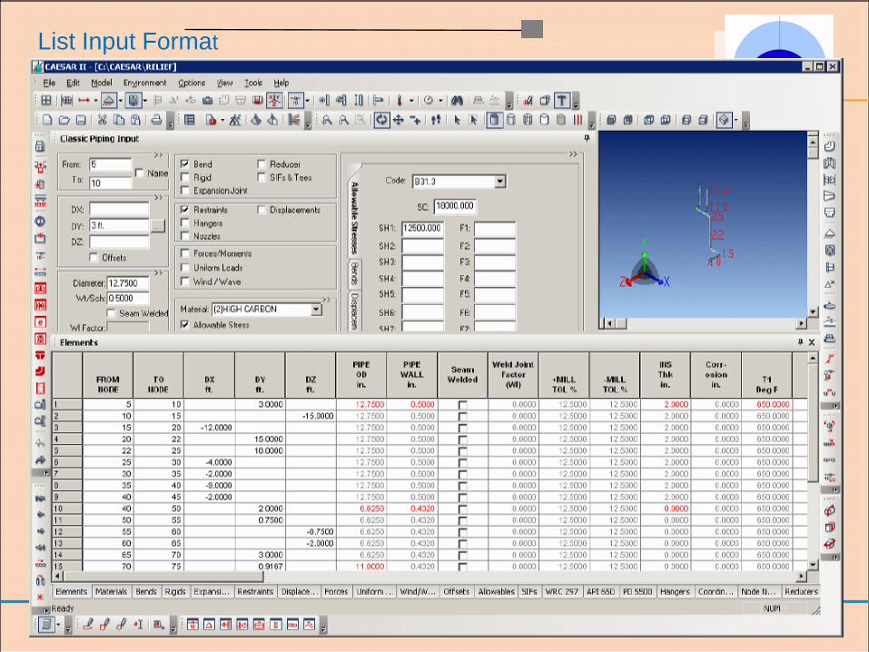
List Input Format
RUNNING THE STATIC ANALYSIS
The static analysis performed by CAESAR II follows the regular finite element
solution routine. Element stiffnesses are combined to form a global system
stiffness matrix. Each basic load case defines a set of loads for the ends of all
the elements. These elemental load sets are combined into system load
vectors. Using the relationship of force equals stiffness times displacement
(F=K∙X), the unknown system deflections and rotations can be calculated. The
known deflections however, may change during the analysis as hanger sizing,
nonlinear supports, and friction all affect both the stiffness matrix and load
vectors. The root solution from this equation, the system-wide deflections and
rotations, is used with the elements‟ stiffness to determine the global (X,Y,Z)
forces and moments at the end of each element. These forces and moments
are translated into a local coordinate system for the element from which the
code-defined stresses are calculated. Forces and moments on anchors,
restraints, and fixed displacement points are summed to balance all global
forces and moments entering the node. Algebraic combinations of the basic load
cases pick up this process where appropriate - at the displacement, force &
moment, or stress level.
Once the setup for the solution is complete the calculation of the displacements
and rotations is repeated for each of the basic load cases.

STRUCTURAL STEEL CHECKS (AISC) Allowable Stress Increase Factor The Allowable Stress Increase Factor is a multiplication factor applied to the
computed values of the axial and bending allowable stresses. Typically this
value is 1.0. However, in extreme events the AISC code permits the allowable
stresses to be increased by a factor.
Normally a 1/3 increase is applied to the computed allowables, making the
Allowable Stress Increase Factor = 1.33. Examples of extreme events are
earthquakes and 100 year storms. For more details see the AISC code,
section 1.5.6.
Young’s Modulus The slope of the linear portion of the stress-strain diagram. For structural steel
this value is
usually 29,000,000 psi (199,948 MPa).
Material Yield Strength The specified minimum yield stress of the steel being used.
STRUCTURAL STEEL CHECKS (AISC) (CONT’D.)
Stress Reduction Factors Cmy and Cmz
Cmy and Cmz are interaction formula coefficients for the strong and weak axis of
the elements (in-plane and out-of-plane).
0.85 for compression members in frames subject to joint translation
(sidesway).
For restrained compression members in frames braced against sidesway and
not subject to transverse loading between supports in the plane of bending:
0.6 - 0.4(M1/M2); but not less than 0.4
where (M1/M2) is the ratio of the smaller to larger moments at the ends, of
that portion of the member un-braced in the plane of bending under
consideration.
For compression members in frames braced against joint translation in the
plane of loading and subject to transverse loading between supports, the
value of Cmy may be determined by rational analysis. However, in lieu of such
analysis, the following values are suggested per the AISC code:
a. 0.85 for members whose ends are restrained against rotation in the
plane of bending
b. 1.0 for members whose ends are unrestrained against rotation in the
plane of bending

STRUCTURAL STEEL CHECKS (AISC) (CONT’D.)
Bending Coefficient
The bending coefficient Cb shall be taken as 1.0 in computing the value
of Fby and Fbz for use in Formula 1.6-1a. Cb shall also be unity when the
bending moment at any point in an un-braced length is larger than the
moment at either end of the same length. Otherwise, Cb shall be
Cb = 1.75 + 1.05(M1/M2) + 0.3(M1/M2)2 but not more than 2.3 where
(M1/M2) is the ratio of the smaller to larger moments at the ends.
Form Factor Qa
The form factor is an allowable axial stress reduction factor equal to the
effective area divided by the actual area. (Consult the latest edition of the
AISC code for the current computation methods for the effective area.)
Allow Sidesway
The ability of a frame or structure to experience sidesway (joint
translation) affects the computation of several of the coefficients used in
the unity check equations. Additionally, for frames braced against
sidesway, moments at each end of the member are required.
Normally sidesway is allowed (i.e., the box is checked).
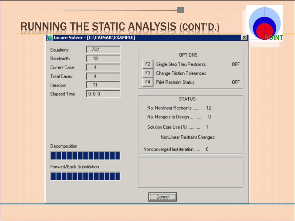
RUNNING THE STATIC ANALYSIS (CONT’D.)

RUNNING THE STATIC ANALYSIS (CONT’D.)
The stress categories:
SUStained,
EXPansion,
OCCasional,
OPErating, and
FATigue
These are specified at the end of the load case definition.
STA
TIC
OU
TP
UT P
RO
CE
SS
OR
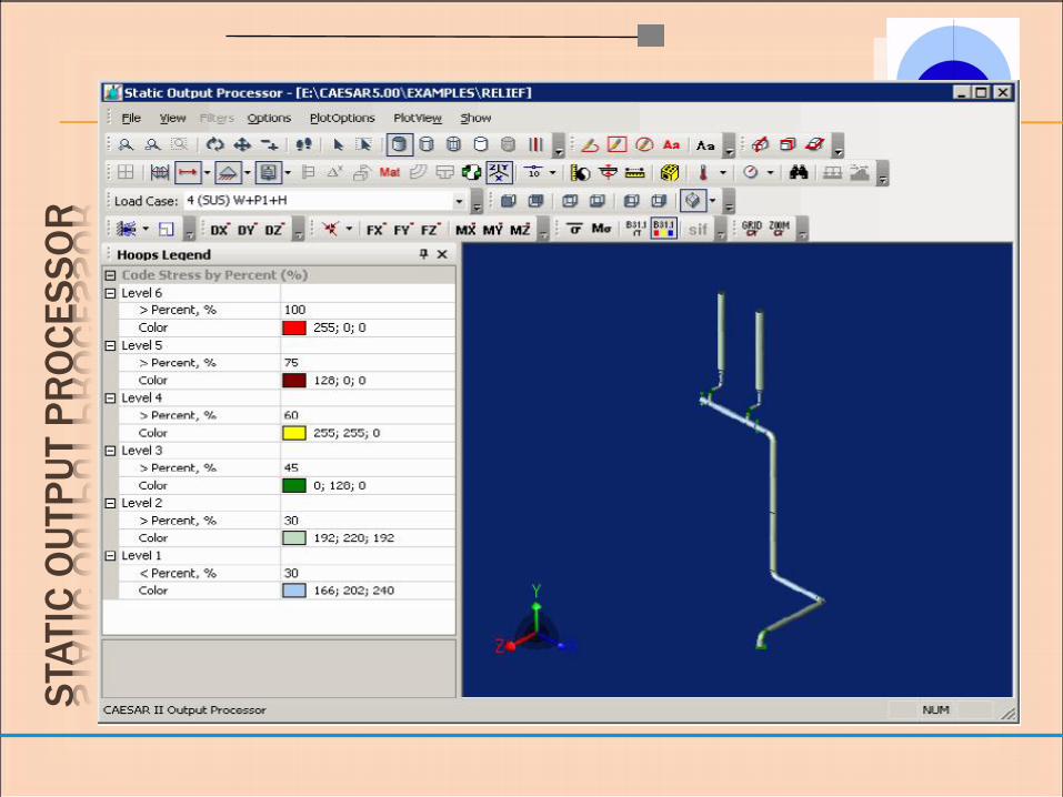
STATIC ANALYSIS OUTPUT
User defined retained output data
Report Options:
Displacements
Restraints
Restraint summary
Global element forces
Local element forces
Stresses
Stress summary
Code compliance report
Cumulative usage report
The next slide shows the on-screen static output processor.
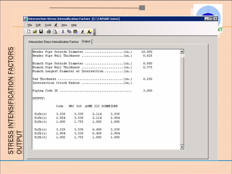
STR
ES
S I
NTE
NS
IFIC
ATIO
N F
AC
TO
RS
OU
TP
UT

DYNAMIC ANALYSIS OF PIPING SYSTEMS
Four types of dynamic analysis are possible:
Natural Frequency calculations
Harmonic analysis
Response Spectrum analysis
Earthquake
[Valve] Relief loads
Water Hammer/Slug Flow
Time History analysis
DYNAMIC ANALYSIS OF PIPING SYSTEMS Caesar II‟s dynamic analysis capabilities include:
Natural Frequency calculations - Natural frequency information can indicate the
tendency of a piping system to respond to dynamic loads. A system‟s modal natural
frequencies typically should not be too close to equipment operating frequencies and, as a
general rule, higher natural frequencies usually cause less trouble than low natural
frequencies.
Harmonic analysis - These are „forcing frequencies‟ that include fluid pulsation in
reciprocating pump lines or vibration due to rotating equipment. These loads are modeled
as concentrated forces or displacements at one or more points in the system. To provide
the proper phase relationship between multiple loads a phase angle can also be
associated with these forces or displacements.
Response Spectrum analysis - The response spectrum method allows an impulse
type transient event to be characterized by a response vs. frequency spectra. Each mode
of vibration of the piping system is related to one response on the spectrum. These modal
responses are summed together to produce the total system response. And
Time History analysis - This is one of the most accurate methods, in that it uses
numeric integration of the dynamic equation of motion to simulate the system response
throughout the load duration. requires more resources (memory, calculation speed and
time) than other methods. spectrum method might be a viable substitute if it offers
sufficient accuracy.
PREPARATION OF MODEL FOR DYNAMIC ANALYSIS
The dynamic analysis techniques employed by many softwares like
Caesar II require strict linearity in the piping and structural systems.
Dynamic responses associated with nonlinear effects are not
addressed.
An example of a nonlinear effect is “slapping”, such as when a pipe
lifts off the rack at one moment and impacts the rack the next. For
the dynamic model the pipe must be either held down or allowed to
move freely. The nonlinear restraints used in the static analysis must
be set to be active or inactive for the dynamic analysis.
A second “nonlinear” effect is friction. Friction effects must also be
“linearized” for use in dynamic analysis. For example, if the normal
force on the restraint from the static analysis is 350 lb., the friction
coefficient (mu) is 0.3, and the user defined Stiffness Factor for
Friction is 50.0, then springs having a stiffness of 350 * 0.3 * 50.0 =
5250 lb/in are inserted into the dynamic model in the two directions
perpendicular to the friction restraint’s line of action.
PREPARATION OF MODEL FOR DYNAMIC ANALYSIS (CONT’D.)
Developing dynamic input for CAESAR II comprises four basic steps:
1) Specifying the load(s)
2) Modifying the mass and stiffness model
3) Setting the parameters that control the analysis
4) Starting and error checking the analysis
To enter the dynamics input, the proper job name must be current prior
to selecting the Analysis-Dynamics file options of the Main Menu.

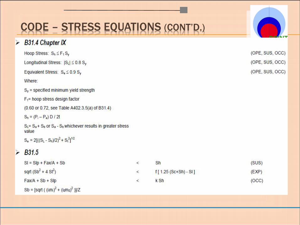
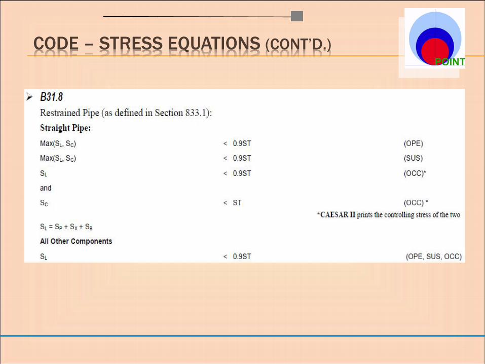
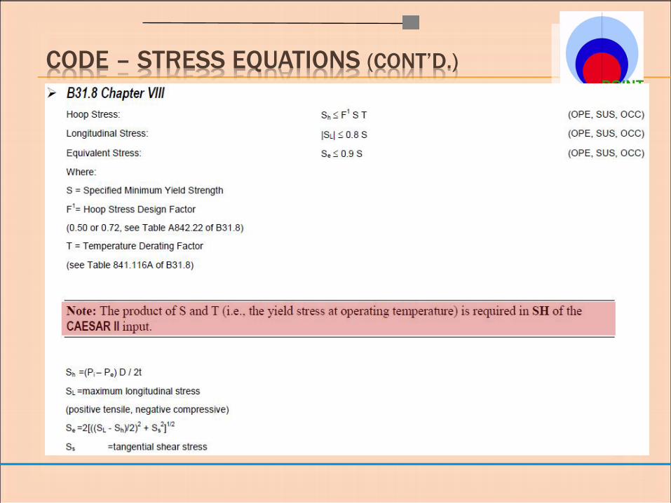
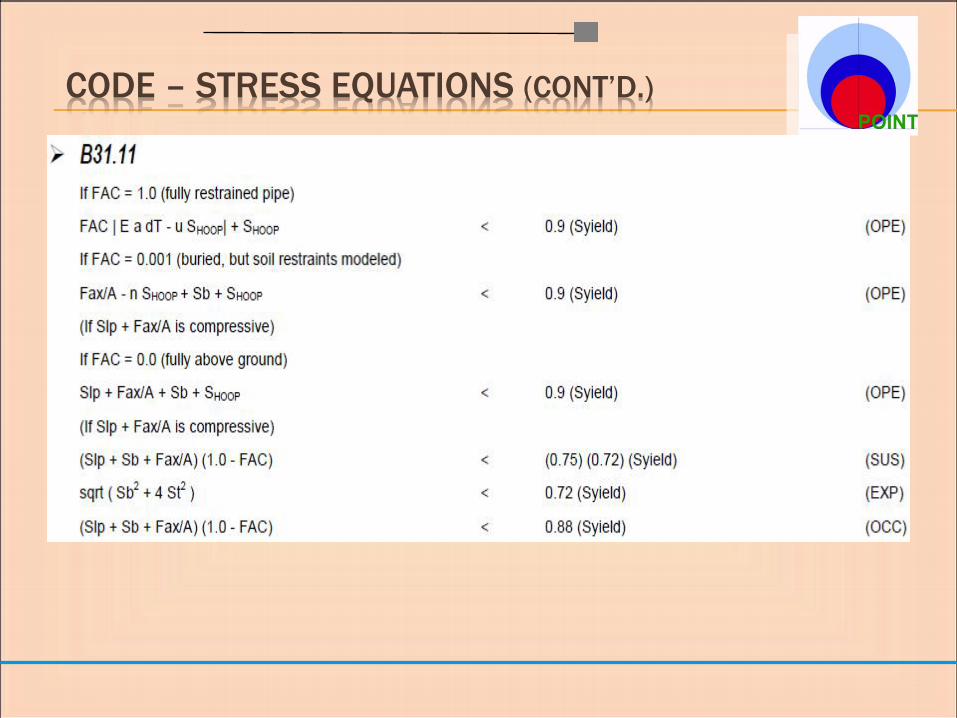
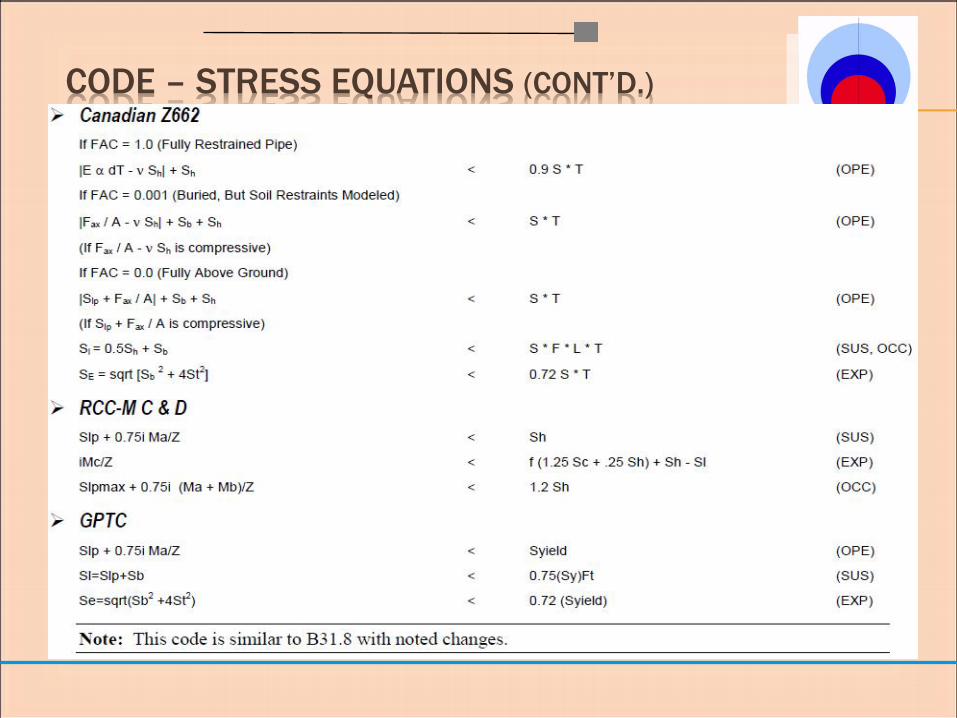
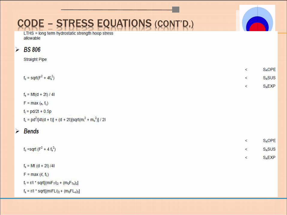
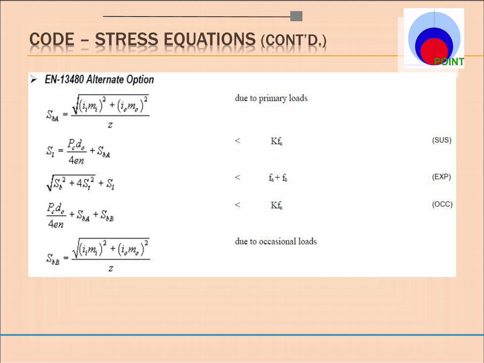
CODE – STRESS EQUATIONS
below are the “code stress” equations for the actual and allowable stresses used
by CAESAR II. For the listed codes, the left hand side of the equation defines the
actual stress and the right hand side defines the allowable stress. The CAESAR
II load case label is also listed after the equation.
US Code Stresses Stress Cat.

CODE – STRESS EQUATIONS (CONT’D.)

CODE – STRESS EQUATIONS (CONT’D.)
CODE – STRESS EQUATIONS (CONT’D.)
CODE – STRESS EQUATIONS (CONT’D.)

CODE – STRESS EQUATIONS (CONT’D.)
CODE – STRESS EQUATIONS (CONT’D.)
CODE – STRESS EQUATIONS (CONT’D.)
CODE – STRESS EQUATIONS (CONT’D.)
CODE – STRESS EQUATIONS (CONT’D.)
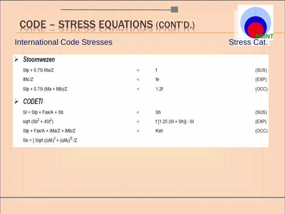
International Code Stresses Stress Cat.
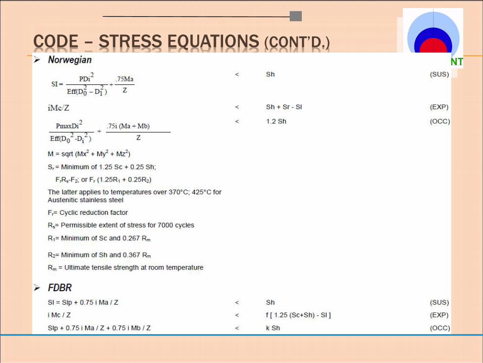
CODE – STRESS EQUATIONS (CONT’D.)
CODE – STRESS EQUATIONS (CONT’D.)
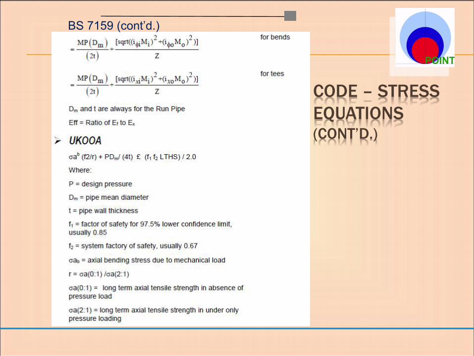
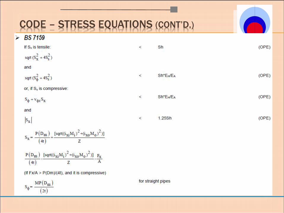
CODE – STRESS
EQUATIONS (CONT’D.)
BS 7159 (cont‟d.)
CODE – STRESS EQUATIONS (CONT’D.)
CODE – STRESS EQUATIONS (CONT’D.)
CODE – STRESS EQUATIONS (CONT’D.)
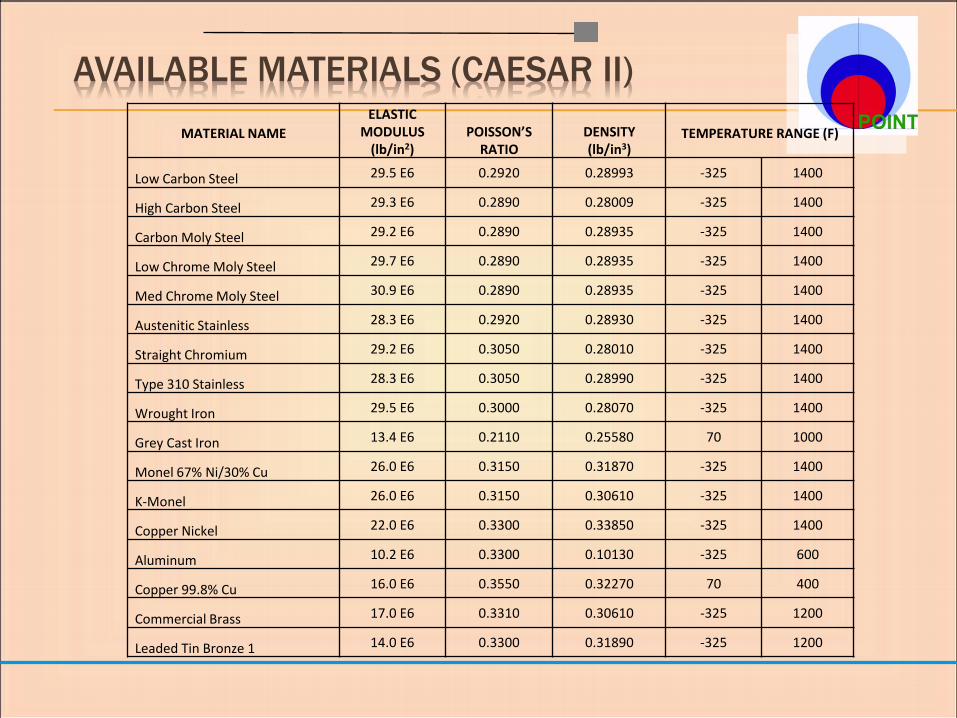
AVAILABLE MATERIALS (CAESAR II)
MATERIAL NAME
ELASTIC MODULUS
(lb/in2) POISSON’S
RATIO
DENSITY
(lb/in3) TEMPERATURE RANGE (F)
Low Carbon Steel 29.5 E6 0.2920 0.28993 -325 1400
High Carbon Steel 29.3 E6 0.2890 0.28009 -325 1400
Carbon Moly Steel 29.2 E6 0.2890 0.28935 -325 1400
Low Chrome Moly Steel 29.7 E6 0.2890 0.28935 -325 1400
Med Chrome Moly Steel 30.9 E6 0.2890 0.28935 -325 1400
Austenitic Stainless 28.3 E6 0.2920 0.28930 -325 1400
Straight Chromium 29.2 E6 0.3050 0.28010 -325 1400
Type 310 Stainless 28.3 E6 0.3050 0.28990 -325 1400
Wrought Iron 29.5 E6 0.3000 0.28070 -325 1400
Grey Cast Iron 13.4 E6 0.2110 0.25580 70 1000
Monel 67% Ni/30% Cu 26.0 E6 0.3150 0.31870 -325 1400
K-Monel 26.0 E6 0.3150 0.30610 -325 1400
Copper Nickel 22.0 E6 0.3300 0.33850 -325 1400
Aluminum 10.2 E6 0.3300 0.10130 -325 600
Copper 99.8% Cu 16.0 E6 0.3550 0.32270 70 400
Commercial Brass 17.0 E6 0.3310 0.30610 -325 1200
Leaded Tin Bronze 1 14.0 E6 0.3300 0.31890 -325 1200
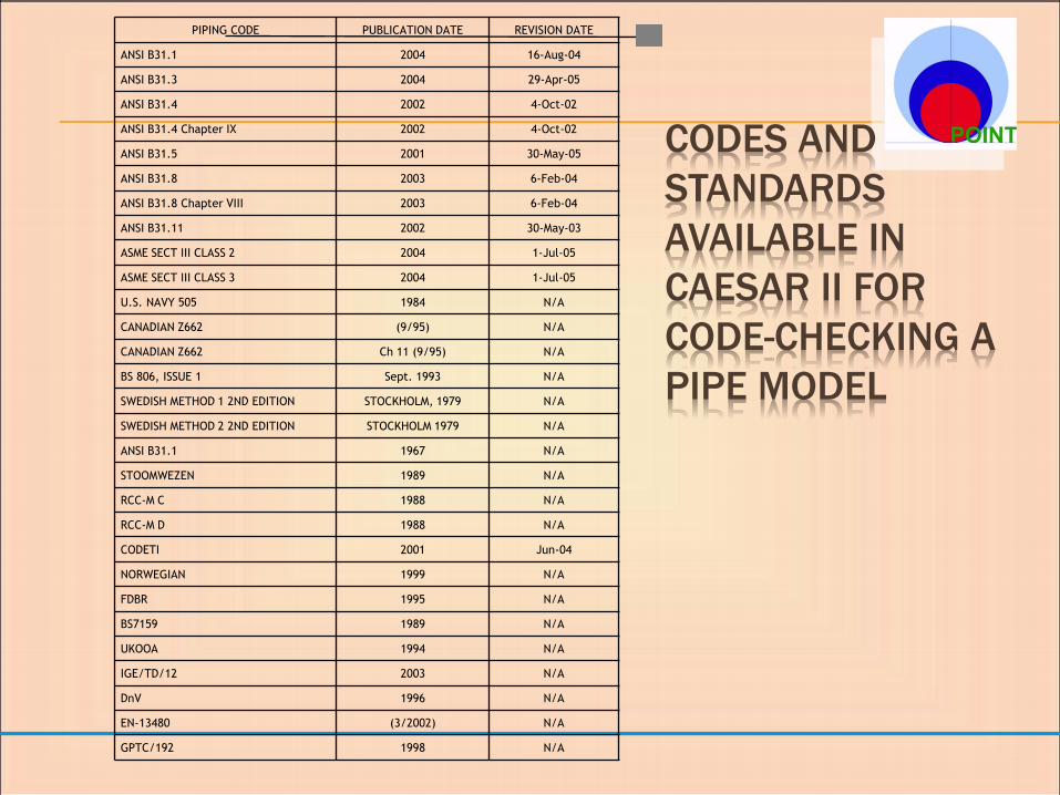
CODES AND
STANDARDS
AVAILABLE IN
CAESAR II FOR
CODE-CHECKING A
PIPE MODEL
PIPING CODE PUBLICATION DATE REVISION DATE
ANSI B31.1 2004 16-Aug-04
ANSI B31.3 2004 29-Apr-05
ANSI B31.4 2002 4-Oct-02
ANSI B31.4 Chapter IX 2002 4-Oct-02
ANSI B31.5 2001 30-May-05
ANSI B31.8 2003 6-Feb-04
ANSI B31.8 Chapter VIII 2003 6-Feb-04
ANSI B31.11 2002 30-May-03
ASME SECT III CLASS 2 2004 1-Jul-05
ASME SECT III CLASS 3 2004 1-Jul-05
U.S. NAVY 505 1984 N/A
CANADIAN Z662 (9/95) N/A
CANADIAN Z662 Ch 11 (9/95) N/A
BS 806, ISSUE 1 Sept. 1993 N/A
SWEDISH METHOD 1 2ND EDITION STOCKHOLM, 1979 N/A
SWEDISH METHOD 2 2ND EDITION STOCKHOLM 1979 N/A
ANSI B31.1 1967 N/A
STOOMWEZEN 1989 N/A
RCC-M C 1988 N/A
RCC-M D 1988 N/A
CODETI 2001 Jun-04
NORWEGIAN 1999 N/A
FDBR 1995 N/A
BS7159 1989 N/A
UKOOA 1994 N/A
IGE/TD/12 2003 N/A
DnV 1996 N/A
EN-13480 (3/2002) N/A
GPTC/192 1998 N/A

REFERENCES
1. COADE, “Version 5.00 CAESAR II
Applications Guide” Caesar II Pipe
Analysis software, www.coade.com (E-
mail at [email protected])
2. British Standard, BS 806, Pipe Bends
3. Water Resources Council (WRC)
Specification 329
4. Caesar II enhancements and reference
topics,
http://www.intergraph.com/products/ppm/
caesarii/enhancements.aspx
5. American Institute of Steel Construction
(AISC), “Steel Construction Manual”, 13th
edition.

END OF PRESENTATION
Related Documents


