User guide

71792 Infinity Users Guide
Dec 29, 2015
c
Welcome message from author
This document is posted to help you gain knowledge. Please leave a comment to let me know what you think about it! Share it to your friends and learn new things together.
Transcript

Use
r g
uid
e


A
B
C
D
E
F
71792 B 2006-04
User guide
Supports Leonova Infinity MMI version 4.0 for Condmaster®Nova 2006 or higher.
G
General instrument functionsInstrument data and functions, general settings, files and upgrades
General measurement functionsMeasurement modes, recording, display windows and spectrum functions
Free measurement techniques Speed, temperature, analogue signals and ISO 2372 vibration
Shock pulse measurementSPM dBm/dBc, SPM HR/LR and SPM Spectrum
Vibration mesurementISO 10816 vibration, FFT with symptoms and EVAM vibration analysisOrbit analysis , Run up /coast down and Bump test
Rotor balancing Single and dual plane balancing
Shaft alignment Horizontal and vertical shaft alignment

TrademarksWindows CE is a trademark of Microsoft Inc.Leonova, CondID, SPM Spectrum and Condmaster are trademarks of SPM Instrument AB.
© Copyright SPM Instrument AB. ISO 9001 certified. Technical data are subject to change without notice.
SPM Instrument ABBox 504, SE-645 25 Strängnäs, SwedenTel +46 152 22500 Telefax +46 152 [email protected] I www.spminstrument.com I www.leonovabyspm.com
This product must be disposed as electronic waste and is marked with a crossed-out wheeled bin symbol in order to prevent it being discarded with household waste.
When once the life cycle of the product is over You can return it to Your local SPM representative for correct treatment, or dispose it together with your other electronic waste.
A
General instrument functions A:�
General instrument functions
Contents
LeonovaTM Infinity, accessories ............................................... 3
Instrument overview .............................................................. 4
Start / Charge batteries ......................................................... 5
Navigation ............................................................................. 6
Reset ...................................................................................... 7
Instrument calibration ........................................................... 7
Main functions ....................................................................... 7
Tools menu ............................................................................ 8
About Leonova ...................................................................... 9
Function and use ................................................................. 10
General settings .................................................................. 12
Select language ................................................................... 14
Set date ............................................................................... 14
Change font, size and style ................................................. 15
Create measurement files .................................................... 15
Register vibration transducer .............................................. 16
Battery status and calibration ............................................. 17
Communication with the PC ................................................ 18
Leonova service program .................................................... 19
Upgrade Leonova software ................................................. 19
Order credits and functions ................................................ 20
Safety copies of Leonova files ............................................. 21
Reload safety copies of Leonova files .................................. 22
File management in Leonova ............................................... 23
List of icons ......................................................................... 24
Technical specifications ....................................................... 25

A:� General instrument functions
A

A
General instrument functions A:�
Leonova Infinity is a multi-function, hand-held data logger. The instrument is operated via keypad and touchscreen. Basic data for the measurement set-up can be input manually or downloaded from Condmaster®Nova.
Leonova Infinity is always programmed for an unlim-ited use of the measuring techniques described in chapter C. Other diagnostic and analytic functions, for shock pulse measurement, vibration measurement, orbit analysis, rotor balancing and shaft alignment, are user selected.
This instruction, SPM 71792, describes the general instrument settings.
Supplied accessories
15178 Stylus for touch screen
14161 Wrist strap
PRO49 Leonova Service Program
71789 Instruction “Getting started”
Optional accessories
90362 Charger, 100-240 V AC, 50-60 Hz, Euro-plug
90379 Charger, 100-240 V AC, 50-60 Hz, US-plug
90380 Charger, 100-240 V AC, 50-60 Hz, UK-plug
CAB46 Communication cable, USB
CAB47 Communication cable RS232, 9 pin
14715 Belt clip
15310 Protective cover
CAS16 Carrying case, plastic with foam insert
The equipment listed above is part of the LeonovaTM instrument. In addition, transducers and measuring cables are needed for the measurements. These are bought separately, depending on which of the avail-able measurement functions are implemented.
CAS16
14715
CAB47
90362 / 90379 / 90380
14661
14649
15310
Leonova™ Infinity
CAB46

A:� General instrument functions
A
Instrument overview
Data
Leonova housing: ABS/PC, Santoprene, IP54Operating temperature: 0 to 50 °C (32 to 122 °F)Charging temperature: 0 to 45 °C (32 to 113 °F)Storing temperature: -10 to 60 °C (14 to 140 °F).
Brackets for stylus on both sides
Position of RF transponder for CondID
Input for shockpulse transducer
Colour touch screen:display of menus
and results, navigation
Wrist strap(fastens left, right)
Input for temperature and tachometer probes, balancing module. Output for earphone.
Input for vibration transducer, max. 18 V peak to peak. Orbit interface.Analog 0 - 20 mA, 4 - 20 mA and 0 - 1 V, 0 - 10 V.
Navigation keys and ENTER
TAB: power on, navigation
MEAS: start measurement
SHIFT: capitals, navigation
Condition indication
SAVE: save measurement
Strap holders
Input for battery chargerPC communication port and input for LineLazer

A
General instrument functions A:�
Leonova is started with the TAB key (1). Start a new instrument with the battery charger connected. POW-ER OFF is automatic. Adjust the date and time under TOOLS, ‘Settings’, ‘Battery status’.
Leonova is powered by a rechargeable lithium-ion bat-tery pack which may only be replaced by authorized service personnel.
The maximum battery capacity is 1800 mAh at 7.4 V. ‘Power low’ warning is given at 6.8 Volt. All functions off at 6.3 Volt.
When battery voltage gets below 6.2 V, the data saved in the RAM memory are lost. It will also stop the clock, making it necessary to reset date and time.
A Connector for battery charger
Only use the SPM Battery Charger. Unless recharged once within 30 days, the Leonova battery pack will be empty (loss of data saved in the RAM memory).
Measuring results are default stored in the flash memory and will not be erased if battery is low.
Note. If the battery is empty, connect the charger and wait at least 2 minutes before pressing any button.
The charger is specified for 100 to 240 VAC, 50 to 60 Hz. Do not use any other type of charger.
Battery loading starts automatically within 30 seconds after connecting. It is normal that the instruments gets warm during loading. A full recharge can take 3 hours.
Check load by clicking on the battery status icon or select TOOLS, ‘Battery status’ (1800 mAh = 100%).
Leonova can be connected to the charger and to the PC at the same time.
Start / Charge batteries
Do not replacethe battery pack!
Refer servicing to your local SPM dealer.
!
Battery status
A
1

A:� General instrument functions
A
Navigation
Key navigation
The navigation keys are TAB, the direction AR-ROWS and ENTER. A keyboard icon is opened with SHIFT + ENTER.
• TAB moves from menu bar to display window to action bar and back. In windows containing several functions, TAB moves through these before jumping to the action bar.
• The ARROW keys move within a bar, a window or a field.
• ENTER opens/activates a highlighted item. It also closes functions and confirms changes.
This is the general rule. Details are explained under the function description.
The Leonova screen is divided into three areas:
• the menu bar (1)• the display window (2)• the action bar (3).
The icons on the menu bar select display win-dows; the buttons and text line on the action bar execute commands.
Touch screen navigation
Leonova can be operated by touch screen alone. To select a function, lightly touch the text or the icon with the stylus or a similar blunt tipped object.
Do not use force; poking hard at the screen can cause damage. In case the function fails to open, use ‘Align screen’ under TOOLS, ‘General settings’.
Please note that, to open a file, you first mark it with the stylus and then touch the ‘Open’ but-ton on the action bar.
�
�
�
tab
measure save
shift

A
General instrument functions A:�
a. FILE: Communication, Read CondID, measurement files saved by the user.
b. SPEED: Speed measurement.
c. SPM: All shock pulse measurement techniques (with SPM Spectrum).
d. VIBRATION: All vibration measurement techniques including orbit analysis, run up/coast down and bump test.
e. ANALOGUE: Temperature and user defined measurements (voltage, current).
f. BALANCING: All rotor balancing techniques.
g. ALIGNMENT: All shaft alignment techniques.
h. TOOLS: General settings.
a b c d e f g h
Main functions The menu bar at the top of the screen opens seven display windows, each containing a number of files. Functions marked grey are not implemented in your Leonova version and can not be opened.
Use TAB to go to the menu bar. Navigate with RIGHT/LEFT, select with ENTER.
In case of instrument malfunction, you should first try to restart Leonova with the software RESET. RAM memory is preserved. A hardware reset erases all data inthe RAM memory.
Do not open the instrument casing. Service on Leonova may only be carried out by specially trained personnel authorized by SPM.
Reset
Software RESET: SAVE + arrow down
Hardware RESET: TAB + SAVE + ENTER
Instrument calibrationAn instrument calibration, e. g. for the purpose of com-pliance with ISO quality standard requirements, is rec-ommended once per year. The calibration is made at the Authorized Service Establishments.
The calibration reminder icon (1) in the lower right cor-ner of the display shows when the Leonova is used for the recommended period and is to be sent to a by SPM authorized service establishment in your local area.
1

A:� General instrument functions
A
Tools menu
The nine files under TOOLS contain the general instru-ment settings. With a new Leonova, the first task is to check the available functions and to adjust the instru-ment. These are the files:
1. General settings, a menu for several functions.
Select units: the default is mm, °C, Hz.
Icons: show large/small icons.
Layout: measuring point tree layout and ‘Preview live spectrum’.
Balancing: select ounce, counter rotational degrees and output unit (ACC, VEL, DISP).
Communication: Selection of USB port or baud rate and COM port for RS232 (must conform with Cond-master and computer settings).
Screen: Align screen. Adjust brightness and back light.
Automatic save: Prompt to save after measurement.
2. Language: Choose among available languages.
3. Date/time: Adjust when needed.
4. Vibration transducers: Register your transducer(s). Attention! All values must be taken from the transducer’s calibration card.
5. Fonts: Select text presentation.
6. Create default files: Creates the initial files needed to use the measuring functions.
7: Function and use: Shows available functions, credits needed for loaded measuring rounds, credit tank data.
8. Battery status: Calibrate. Adjust time for automatic power off.
9. About Leonova: Software version data and serial number.
� � �
� � �
� � 9

A
General instrument functions A:9
About Leonova
The file ‘About Leonova’ contains important informa-tion on the software status.
Program versions:MMI Leonova software, user interface.Math Leonova software, algorithms
Firmware Leonova interface to Windows CEFPGA Leonova signal condition software
Customer data:License number Individual license for the instrment
Package number Running number of update opera-tions.
The Leonova software, ‘MMI’ and ‘Math’, is contained in the file ‘P70.exe’. The file ‘FPGA.P70’ con-tains the signal condition software.
The license number belongs to the instrument. All upgrades concerning program versions, func-tions and credits are connected with it.
When ordering new functions and/or credits, these are delivered as a text file ‘Leonova.txt’. Each such order has a running package number and is individual for the instrument. The files can only be loaded in package order, see ‘Leonova Service program’.

A:�0 General instrument functions
A
Function and use
Leonova has a number of ‘platform’ functions which are always available with unlimited use. Other func-tions are user selectable and can be bought with either unlimited or limited use.
‘Function and use’ under TOOLS shows a list of all functions, each followed by an icon showing its status:
The ‘refill’ icon marks the functions where credits are deducted from the credit tank each time the MEASURE command is given.
Loaded measuring rounds are shown at the bottom of the list.
Available, unlimited use.
Available, credits required.
Not available in this instrument.
Touching this icon shows the number of credits required for the marked function (1) or measuring round (2).
�
�

A
General instrument functions A:��
Touching this icon shows the credit tank data and status. Some of the listed items can be edited.
Mark a line and touch the edit button. ‘Tank size’ is selected from a list.
The emergency tank size is fixed to 250, and the emergency tank factor to 2. When using the emer-gency tank, 2 credits will be deducted instead of 1. It is therefore advisable to order a refill in good time.
The last three lines can be edited, both warning texts and values. Touching ‘Edit’ first opens the text. Change or touch OK to continue to the value.
The loading of new credits and functions is de-scribed under ’Leonova service program’.
Functions for Limited Use (Function & Use) Credit consumption
LEO230 Shock pulse method dBm/dBc 1
LEO231 Shock pulse method LR/HR 2
LEO232 SPM Spectrum 2
LEO233 ISO 10816 vibration monitoring with spectrum 1
LEO234 FFT with symptoms 2
LEO235 EVAM evaluated vibration analysis, time signal 2
LEO236 2 channel simultaneous vibration monitoring 4
LEO237 Run up / coast down (50) and Bump test 25
LEO238 Orbit analysis 5
LEO252 Balancing, single plane, 4 runs 16
LEO252 Balancing, single plane, 2 runs 42
LEO253 Balancing, dual plane 80
LEO255 Shaft alignment 30

A:�� General instrument functions
A
General settings
The files under TOOLS cannot be moved, renamed or deleted.
‘General settings’ has its own menu bar (1).
Marking the box (2) changes from mm to inch, from °C to °F and from Hz (Hertz = cycles per second) to CPM (cycles per minute, similar to rpm).
When ‘Large icons’ (3) is not marked, files are listed as shown above (4).
This selection (5) affects the measurement window. ‘Measuring point name . .’ re-peats the name on a separate line. ‘Col-our’ displays the evaluation icon for each listed measuring technique. ‘Automatic save’ opens a small ‘Save yes - no’ window immediately after a measurement. ‘Use temporary file’ will save the round tem-porary while saving. ‘Live spectrum’ will show spectrum in real time.
The selections under (6) concern ‘Balanc-ing’.
‘Counter rotational degrees’ means that angles are measured opposite to the direction the rotor is moving.
‘Ounce’ changes weights from grams to ounces. ‘Output unit’, selected from a list, is the unit of the vibration measurement (acceleration, velocity or displacement).
�
�
�
�
�
�

A
General instrument functions A:13
‘Communication’ is used to select port on the PC, USB or COM port.
Please check that the Leonova settings agree with the configuration of your PC and with the settings in CondmasterNova.
A mismatch of settings is often the cause of a commu-nication fault message when trying to download data from the PC.
‘Align screen’ (1) is used when functions fail to open on touch.
Touch and drag
You come to a window showing a cross (+). Touch and hold its centre until the cross moves to the next of its five positions on the screen. Finish with ENTER.
For ‘Backlight ON’ (2), you can change backlight brightness by dragging the regulator with the stylus (or the LEFT/RIGHT arrow keys).
Selecting ‘AUTO’ opens a regulator (3) for setting the backlight switch off time (5 to 99 seconds).
Open the keyboard by either touching it or by moving to the number field with TAB and pressing SHIFT+ENTER.
Touch the desired numbers one by one. You can erase with ← (one step) or with ‘C’ (all). To cancel, touch ‘X’. To finish, touch √. When using the keys, navigate to the desired number/sign with the arrow keys, then select it with ENTER.
1
2
3

A:�� General instrument functions
A
Set date
When the battery is empty, Leonova no longer updates the clock. To be able to communicate with the PC, Leonova’s time and date setting must be within 5 minutes of the computer’s time and date.
The fastest way of resetting the Leonova clock is to import time and date from the PC while downloading a measuring round.
To make the update directly on Leonova, mark the value field, touch the keyboard and write the new time/date, using the standard format.When navigating by keys, TAB will change between the fields for time and date; SHIFT+ENTER will open the keyboard.
Select language
The file ‘Language’ under TOOLS allows you to choose among the available Leonova screen lan-guage. To change to another language, mark this language, then touch the ARROW button (1).
With EDIT (2) you open the complete list of Leonova screen texts (3) for the marked language. You can open any line by marking it and touching EDIT (4). To change the text, open the keyboard, overwrite the existing text and touch OK. The COPY button (5) copies the marked language and saved it under a new name.
Please note:The language editing functions in Leonova are nor-mally not used. Translations are made with the Leono-va Emulator, and new languages are loaded via the Leonova Service program.
�
�
�
��

A
General instrument functions A:��
Create measurement files
The file ‘Create default settings’ under TOOLS is very important. It creates measurement files for all measuring techniques and places them under the measuring technique windows. You cannot use Leonova as a stand-alone measuring instru-ment without these files.
The installation is simple: Open ‘Create default settings’, touch OK.
The example shows the measurement files cre-ated in the vibration technique window: a file for EVAM and a file each for vibration measurement according to ISO 10816 and ISO 2372.
Change font, size and style
The ‘Fonts’ menu ‘ allows you to make individu-al changes of font, style and size for any of the listed alternatives (1).
When showing file names, Leonova uses the largest text that fits into the available space, going from ‘Normal’ (16 points) via ‘Medium’ (14 points) to ‘Small’ (12 points). Thus, if you have difficulties reading ‘Small’ text, you can change the text size of ‘Small’ from 12 to 14 points.
Leonova will truncate file names that are too large to fit on one line. Using several words or hyphens in the name will put it on two or more lines.
Marking an item on the list and touching EDIT (2) opens the window (3) where you can set character size and/or select another font (4) for the item. Please note that this will not affect the other items.
‘Save default settings’ (5) will reset all items to default values.
�
�
�
� �

A:�� General instrument functions
A
Register vibration transducer
The default SPM vibration transducer for Leonova is SLD144. The instrument can also work with any other transducer of IEPE (integrated electronic piezoelectric) type with voltage output.
Transducers of not IEPE type which do not require power supply, like velocimeters, can also be used. The ‘IEPE type’ has then to be set to ‘No’.
Vibration transducers must be registered under TOOLS, ‘Vibration transducers’. The active transducer is selected by marking a transducer name and touching the arrow (3).
To register a transducer, touch NEW (1), then inputthe following data:
Name: A descriptive name. It will be shown on the list of transducers.
Type: The measured vibration parameter, ei-ther ACC (acceleration), VEL (velocity) or DISP (displacement).
Sensitivity: The transducer’s nominal sensitivity in the displayed unit (which depends on the input under ‘Type’).
Max. frequency: The transducer’s upper frequency range.
IEPE type: YES or NO. ‘Yes’ opens the next three lines.
Min. bias range: The lower working voltage.
Max. bias range: The upper working voltage.
Settling time: Stabilizing time for the transducer after ‘power on’.
The min. and max. bias voltage is needed for the TLT test (transducer line test, returning ‘Interrupted circuit’ when the measured voltage is above the max. bias voltage, and ‘Short circuit’ when it is below the min. bias voltage.
To select default transducers for the balancing function, press the button (4) ‘Balancing transducers’ and register two transducers to be used. Default transducers for orbit analysis (5) and for 2 channel vibration monitoring (6) are registered in same way.
To change transducer data, use the EDIT button (2).
�� �� � �
�
�
�

A
General instrument functions A:��
Battery status and calibration
The file ‘Battery status’ shows the remaining charge in percent (1). The battery is calibrated on delivery.
In case you suspect that the battery status display is out of kilter, use the button ‘Discharge/Charge’ to re-calibrate.
• Connect Leonova to the battery charger.
• Touch the button ‘Discharge/Charge’.
• Wait for about two minutes, then touch ‘OK’.
Leave Leonova connected to the charger over night. Do not touch any buttons or keys except TAB until the procedure ends and Leonova is charged to 100%. It is recommended to start with a low bat-tery charge, because discharging takes about 10 hours for a fully charged battery.
To set the time delay before automatic power off (2), open the keyboard and set a number between 20 and 300 seconds.
�
�

A:�� General instrument functions
A
Communication with the PC
Leonova connects to the PC via the communication cable CAB46 for an USB port or CAB47 for a 9 pin COM port (RS232).
Leonova communicates with
• Leonova Service Program.• Condmaster®Nova 2006
Place both programs into the same folder on your PC.
To start communication, select ‘Communication’ under the ‘. . .’ button (1) or go to the Leonova ‘File’ menu and open the file ‘Communication’ (2).
On the PC, open ‘Data transfer’ or ‘Planning’ in Condmaster.
Windows 2000 requires a driver for USB communi-cation. The driver can beloaded from the Service Program CD.
CAB46CAB47
COM USB
�
�

A
General instrument functions A:�9
Leonova service program
The Leonova Service Program is used to
• print balancing and alignment reports.• load credits and/or functions from the file
‘Leonova.txt’.• transfer language files from file ‘*.llf’. • upgrade a Leonova version from the file
‘P70.EXE’.• upgrade FPGA software from a file called
‘FPGA.P70’.• display and print a credit log containing
all measurements for which credits were deducted, up to 10000.
• make and reload safety copies of the Le-onova files (file extension .lsc).
Upgrade Leonova software
The latest version of the Leonova soft-ware can be downloaded from the SPM Homepage:
• www.spminstrument.com.
Open ‘Support’, ‘Software update’ and ‘Leonova software’. Download the file ‘P70.EXE’ to your PC.
To upgrade Leonova,
• Open ‘Communication’ on the instru-ment.
• Connect Leonova to the PC.• Start the Leonova Service program on
the PC.• Select ‘Upgrade Leonova software’.• Input the path to the file ‘P70.exe’ and
click CONTINUE.

A:�0 General instrument functions
A
Order credits and functions
Order credits and functions from your SPM supplier. You will receive the text file Le-onova.txt. It is coded to the instrument’s license and also contains a running package number. The files have to be loaded in pack-age number order.
Connect Leonova to the PC and use ’Load functions/credits to Leonova’ to transfer the file contents.
Credits have the ordering number LEO290. Functions ordered after buying Leonova Infinity have one set of numbers for unlimited use (list A) and another for limited use (list B).
‘Credit log’ shows a log of all actions con-cerning credits, up to 10000.
A. Functions for unlimited use
LEO130 Shock pulse method dBm/dBcLEO131 Shock pulse method LR/HRLEO132 SPM SpectrumLEO133 ISO 10816 vibration monitoring with
spectrumLEO134 FFT with symptomsLEO135 EVAM evaluated vibration analysis,
time signalLEO136 2 channel simultaneous vibration
monitoringLEO137 Run up / coast down & bump testLEO138 Orbit analysisLEO151 Shock pulse method dBm/dBc and
LR/HRLEO152 Balancing, single planeLEO153 Balancing, dual planeLEO154 Balancing, single and dual planeLEO155 Shaft alignment
B. Functions for limited use (Function & Use)
LEO230 Shock pulse method dBm/dBc (1)LEO231 Shock pulse method LR/HR (2)LEO232 SPM Spectrum (2)LEO233 ISO 10816 vibration monitoring with
spectrum (1)LEO234 FFT with symptoms (2)LEO235 EVAM evaluated vibration analysis,
time signal (2)LEO236 2 channel simultaneous vibration
monitoring (4)LEO237 Run up / coast down (50) and Bump
test (25)LEO238 Orbit analysis (5)LEO251 Shock pulse method dBm/dBc and
LR/HR LEO252 Balancing, single plane (4 runs 16, 2
runs 42) LEO253 Balancing, dual plane (80)LEO254 Balancing, single and dual planeLEO255 Shaft alignment (30)
Credit consumption is stated within brackets.
Optional functions for unlimited use
LEO139 12 800 lines, 40 kHzLEO160 Recording functionLEO161 Extended memory, 512 MBLEO162 Extended memory, 1 GBLEO163 Extended memory, 4 GBLEO164 Time signal, option to FFT with
symptoms

A
General instrument functions A:��
Safety copies of Leonova files
The Leonova Service program is also used to make safety copies of all measurement files saved in Leonova, and to reload these files to Leonova when needed. Leonova safety copies must have the extension ‘lsc’; the rest of the file name is your choice.
To make a safety copy,
• Connect Leonova to the PC.
• Open ‘Communication’ on the instrument.
• Start the Leonova Service pro-gram on the PC.
• Select ‘Safety copy’, click CON-TINUE.
• Select a folder on your PC, e.g. your Condmaster folder, and click SAVE.
When reloading from a safety copy, there are two alternatives, all files or a single file. The single file option can be used to transfer a meas-urement file from one Leonova to another, and from there to CondmasterNova.

A:�� General instrument functions
A
To reload a safety copy,
• Connect Leonova to the PC.
• Open ‘Communication’ on the instru-ment.
• Start the Leonova Service program on the PC.
• Select ‘Reload safety copy’.
• Select the file to be loaded, click OPEN.
• Select ‘Reload all files’ or ‘Reload single file’. ‘All files’ will erase the present files on Leonova. Continue with YES when you get the warning. For ‘Single file’ you get a file list where you make your selec-tion and click OK.
Reload safety copies of Leonova files
The selection ‘View safety copy’ displays information on
• Leonova version• Credit tank status, and• Function status.
For the function ‘Recording’, the status is either ‘Yes’ or ‘No’ (available or not). For all other functions, the alternatives are
• Free use• Refill (credits deducted when used)• Disabled.
Disabled function can be bought, and ‘re-fill’ functions can be turned into ‘free use’ functions
A
General instrument functions A:��
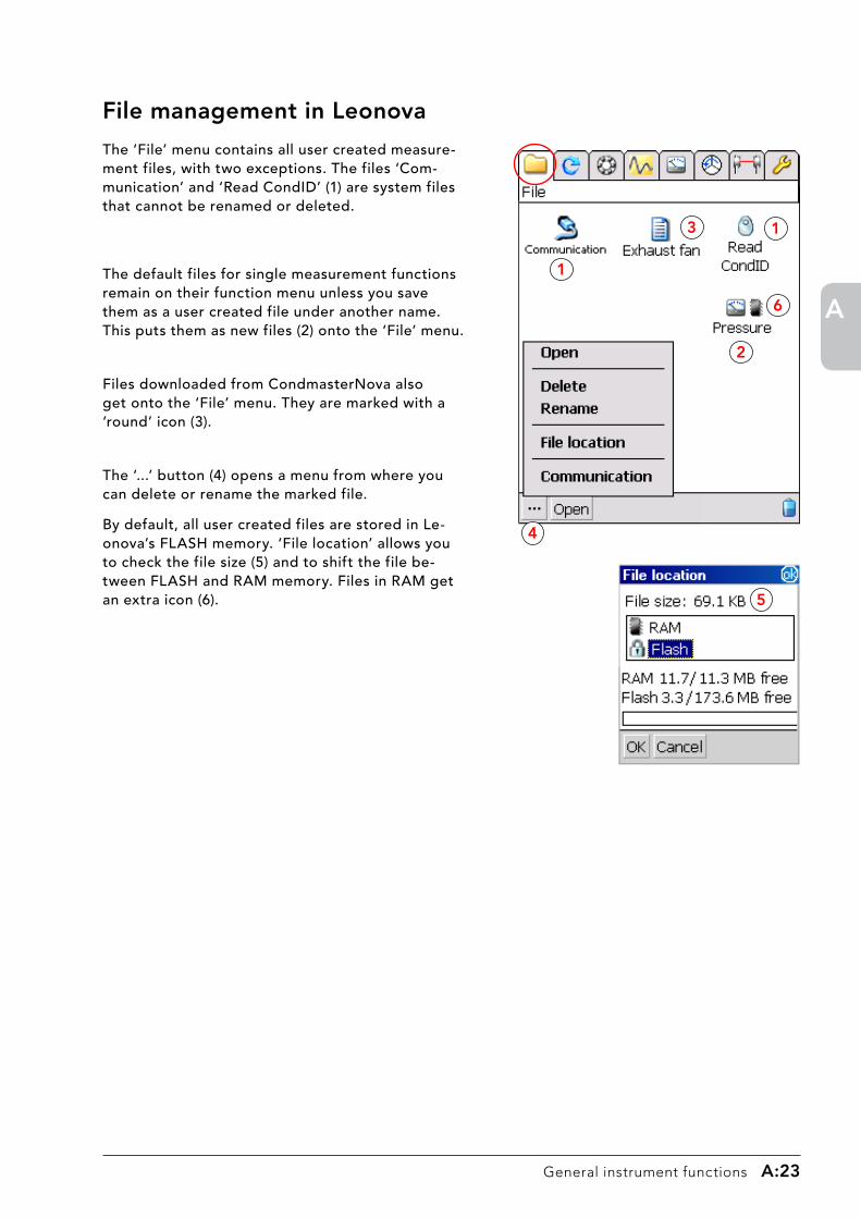
File management in Leonova
The ‘File’ menu contains all user created measure-ment files, with two exceptions. The files ‘Com-munication’ and ‘Read CondID’ (1) are system files that cannot be renamed or deleted.
The default files for single measurement functions remain on their function menu unless you save them as a user created file under another name. This puts them as new files (2) onto the ‘File’ menu.
Files downloaded from CondmasterNova also get onto the ‘File’ menu. They are marked with a ‘round’ icon (3).
The ‘...’ button (4) opens a menu from where you can delete or rename the marked file.
By default, all user created files are stored in Le-onova’s FLASH memory. ‘File location’ allows you to check the file size (5) and to shift the file be-tween FLASH and RAM memory. Files in RAM get an extra icon (6).
��
�
�
�
�
�

A:�� General instrument functions
A
List of icons
1. Go to main function FILE.2. A file, e. g. a measuring round.
1. Go to main function SPEED.2. A speed measurement.
1. Go to main function SPM.2. An SPM technique.
Go to main function VIBRATION.
1. Go to main function ANALOG.2. An analog measurement.
Go to main function BALANCING.
Go to main function ALIGNMENT.
Go to main function SETTINGS.
General setting (units, Baud rate, icons, screen).
Language selection for Leonova screen texts.
Vibration transducer register.
Open default files for measuring tech-niques.
Measuring credits, available functions.
Check battery status, set power down time.
Battery status, power down now.
Communication with PC. CondID memory tag functions.
File saved in RAM. Create new.
Edit.
Keyboard for input of text and numbers.
Manual input of measuring results.
Vibration measurement, ISO 10816.
Vibration measurement, ISO 2372.
SPM Spectrum measurement.
Vibration measurement, EVAM.
2 channel vibration measurement
Show measuring point data.
Browse through measurements.
Show measuring results.
Show measuring result diagram.
Show spectrum.
Show time record.
Good condition (green).
Condition warning (yellow).
Bad condition (red).
Good condition, but above alarm limit. Condition not evaluated.
Alarm limit exceeded.
Measurement completed.
Earphone connected. Change volume.
Balancing, single plane, 2 runs.
Balancing, dual plane.
Balancing, single plane, 4 runs.
Horizontal shaft alignment.
Vertical shaft alignment.
Orbit analysis
Run up / Coast down
Bump test
Calibration reminder
Information.

A
General instrument functions A:��
Technical data, instrument
Housing: ABS/PC, Santoprene, IP54
Dimensions: 285 x 102 x 63 mm
(11.2” x 4” x 2.5”)
Weight: 580 g (20 oz.)
Keypad: sealed, snap action
Display: touch screen, TFT colour,
240 x 320 pixels, 54 x 72 mm
(2.1 x 2.8 inch), adjustable backlight
Main processor: 400 MHz Intel® XScale®
Memory: 64 MB RAM, 32 MB Flash expandable up to 4 GB
Operating system: Microsoft Windows® CE.net
Communication: RS232 and USB
Dynamic range: 16 bit A/D converter, auto-matic gain settings
Condition indication: green, yellow and red LEDs
Power supply: rechargeable Lithium-Ion batteries
Battery power: for min. 8 hours normal use
Operating temperature: 0 - 50 °C (32 - 120 °F)
Charging temperature: 0 - 45 °C (32 - 113 °F)
General features: language selection, trans-ducer line test, metric or imperial units
Meas. point identification: RF transponder for com-munication with CondIDTM tags, read/write distance max. 50 mm (2 inch)
Speed measurement
Measuring range: 10 - 60 000 rpm
Resolution: 1 rpm
Accuracy: ± (1 rev. + 0.1% of reading)
Transducer type: TAD-18, TTL-pulses
Temperature measurement
Measuring range: -50 - 440 °C (-58 - 824 °F)
Resolution: 1 °C (1 °F)
Transducer type: TEM-11 with TEN-10 (surface temperature) and TEN-11 (liquids)
Analog signals
Measurement range: 0 - 1 V DC, 0 - 10 V DC, 0 - 20 mA, 4 - 20 mA
Shock pulse method dBm/dBc
Measuring range: –9 to 99 dBsv
Resolution: 1 dBsv
Technical specifications
Accuracy: ± 1 dBsv
Transducer type: SPM 40000/42000, probe transducer and quick connector transducer for adapters
Input data: rpm, shaft diameter (or ISO bearing number)
Output: maximum value dBm, evalu-ated green - yellow -red; carpet value dBc; peak value, audible shock pulse signal (earphones).
Shock pulse method LR/HR
Measuring range: –19 to 99 dBsv
Resolution: 1 dBsv
Accuracy: ± 1 dBsv
Transducer type: SPM 40000/42000, probe transducer and quick connector transducer for adapters
Input data: rpm, plus bearing type and mean diameter (or ISO bearing number)
Output: LR and HR (raw shock values), CODE A to D, evaluated green-yellow -red. LUB no. for oil film condition, COND no. for surface condition.
SPM Spectrum
Frequency range: 0 to 100, 200, 500, 1000, 2000, 5000, 10 000, 20 000 (40 000) Hz
Spectrum lines: 400, 800, 1600, 3200, 6400 (12800)
Meas. windows: Rectangle, Hanning, Hamming, Flat Top
Spectrum types displayed: linear, power
Averages: time synchronous, FFT linear, FFT peak-hold
Frequency units: Hz, CPM
Saving options for spectrum: full spectrum, peaks only
Amplitude unit: SD (Shock Distribution), SL (Shock Level)
Scaling: linear or logarithmic X and Y axis
Zoom: true FFT zoom, visual zoom
Pattern
recognition: bearing frequencies and option-al patterns highlighted in the spectrum. Automatic config.of bearing symptoms linked to ISO bearing no.
Transducer type: shock pulse transducers with probe and quick connector, SPM 40000/42000
* Integral Electronic PiezoElectric

A:�� General instrument functions
A
Vibration severity (ISO ����)
Measurement quantity: velocity, RMS value in mm/s over
10 to 1000 Hz
Evaluation table selection: menu guided, ISO 2372
Transducer input: < 18 Vpp. Transducer supply of 4 mA for IEPE* (ICP) type can be set On/Off
Transducer types: vibration transducer SLD144 or IEPE (ICP®) type transducers with voltage output
Vibration channels: 2, multiplexed (simultaneous as option)
Vibration (ISO �0��� with spectrum)
Measurement
quantity: velocity, acceleration, and dis-placement, RMS values over 2, or 10 Hz to 1000 Hz, peak, peak-to-peak
Spectrum, linear, 1600 lines, Hanning win-dow.
Spectrum unit: velocity, mm/s or inch/s
Transducer type: vibration transducer SLD144 or IEPE* (ICP®) type trans-ducers with voltage output
FFT spectrum and EVAM Evaluated vibration analysis
Frequency limit, lower: 0.5, 2, 10 or 100 Hz
Frequency limit, upper: 100, 200, 500, 1000, 2000, 5000,
10 000, 20 000 (40 000) Hz
Envelope high pass filters: 100, 200, 500, 1000, 2000, 5000,
10 000 Hz
Measurement windows: Rectangle, Hanning, Hamming,
Flat Top
Averages: time synch, FFT linear, FFT expo-nential, FFT peak-hold
Spectrum lines: 400, 800, 1600, 3200, 6400 (12800)
Frequency units: Hz, CPM, orders
Saving options for spectrum: peaks only, full spectrum, time
signal
Spectrum types displayed: linear, power, PSD
Zoom: true FFT zoom, visual zoom
Transducer type: vibration transducer SLD144 or IEPE (ICP®) type transducers with voltage output
Technical specificationsRun up/coast down
Frequency limit, lower: 0.5, 2 10 or 100 Hz
Frequency limit, upper: 1 to 9999 orders
Measuring interval: speed or time based
Measurement windows: Rectangle, Hanning, Hamming, Flat Top
Spectrum lines: 400, 800, 1600, 3200, 6400, 12800
Spectrum types displayed: linear
Bump test
Frequency limit, lower: 2 Hz
Frequency limit, upper: 100, 200, 500, 1000, 2000, 5000, 10 000, 20 000, 40 000 Hz
Spectrum lines: 400, 800, 1600, 3200, 6400, 12800
Spectrum types displayed: linear
Pre-trigger time: 5%, 10%, 20%, 25% of sampling time
Transducer types: Vibration transducer SLD144 or IEPE* (ICP®) type transducers with voltage output
Orbit analysis
Orders: 1 to 5, default 1
Filter types: none, band pass, low pass
Signal unit: DISP, VEL, ACC
Trig threshold: automatic
Measuring time: 1 to 25 revolutions
RPM range: 15 to 20 480 rpm
Transducer types: buffered outputs from API670 approved protection systems via Orbit Interface 15315, alternative vibration transducers SLD144 or IEPE (ICP®) type transducers with voltage output
* Integral Electronic PiezoElectric
Specifications are subject to change without notice.

General measurement functions B:�
B
Contents
Leonova measurement functions ........................................... 3
Measuring modes .................................................................. 3
Measurement with default files ............................................. 4
Measurement with edited default files .................................. 5
Single measurement user files ............................................... 6
Default file for reading CondID tags ..................................... 6
Multi measurement user files ................................................ 7
Recording ............................................................................. 8
Measuring rounds from Condmaster ..................................... 9
Measuring rounds for CondID ............................................. 10
The measuring sequence ......................................................11
Measurement window before measuring ............................. 12
Measurement window before saving ................................... 13
Comments ........................................................................... 14
Graphics window ................................................................. 15
Measuring result window ..................................................... 16
Live spectrum window ......................................................... 17
Spectrum window ................................................................ 18
Spectrum functions.............................................................. 19
Spectrum functions on the ‘Settings menu’ ........................ 21
Highlighted symptoms in the spectrum ............................... 23
Multi line symptoms with harmonics .................................... 25
Waterfall diagram ................................................................ 27
Phase spectrum ................................................................... 28
The time signal .................................................................... 29
General measurement functions

B:� General measurement functions
B

General measurement functions B:�
B
Leonova measurement functions
Leonova™ Infinity always has the following measurement functions with unlimited use:
• Speed measurement, rpm and peripheral• Temperature measurement• Measurement of analog signals as current and voltage• RMS vibration measurement according to ISO 2372.
The remaining measurement functions are user selected, with either limited or unlimited use:
• Vibration measurement according to ISO 10816, with spectrum• FFT with symptoms• EVAM evaluated vibration analysis• Shock pulse measurement• SPM Spectrum• Run up/Coast down and Bump test• Orbit analysis• Balancing• Shaft alignment
Measuring modesLeonova is primarily designed as a data logger. Measuring rounds, complete with all input data for evaluated measurements, are downloaded from a PC running the SPM software Condmaster®Nova. After measurement, the results are uploaded to the PC.
When data logging, the operator works along a predetermined route and measures ‘in round or-der’. As an alternative, CondID memory tags can be attached to the machines. A measuring point, belonging to a downloaded measuring round, is identified by reading its tag. Leonova Infinity displays that point and its data, ready for measurement.
For unprepared measurement, Leonova contains a ‘default file’ for each measuring technique. When required, the input data are entered manually by editing the default values. Edited default files can be saved as new default files, or as user files which retain both the input data and the measuring results
For each measurement, the user can input a comment.
When implemented, the function ‘Recording’ can be used to automatically record a stated number of measuring results or measure over a stated time.

B:� General measurement functions
B
Measurement with default files is used for a ‘once only’ check, where you do not need to save the measuring result. Default files are activated with the function ‘Create default settings’ under TOOLS.
• Select a measurement function (1) and one of the default files (2).
• Touch the OPEN button to open the marked default file, then touch the ‘...’ button (3) to get the menu with ‘Measuring point data’ (4).
• The type of measuring point data depends on the measuring method you are using. The window shows default settings (5). Normally, you have to edit these. Mark the line to be edited and touch the EDIT but-ton (6), then change the data using the keyboard. Finish each entry with OK.
• Close ‘Measuring point data’. Connect the transduc-er, measure and save. Saved measuring results can be seen under ‘Graphics’ while the file is still open.
�
�
�
�
Measuring point data, default Measuring point data, edited
6
5
Measurement with default files

General measurement functions B:5
B
Measurement with edited default files
Editing the measuring point data temporarily modifies the default file. In this example, the measured quantity has been changed from ‘4-20 mA’ (the signal) to ‘Flow’ (the quantity repre-sented by the signal), and the measuring unit from ‘mA’ to ‘l/min’. Such changes show up in the measurement window (1).
What happens next depends on how the default file is closed. ‘Close’ (2) simply closes the default file, without saving the edited measuring point data or the measuring results.
To keep the edited measuring point data perma-nently, use ‘Save as’ (3) before closing the file. The choice ‘Save as new default settings’ (4) cre-ates a new default file which you have to name (5).
The edited default file turns up under the meas-urement window (6). It has the same properties as the other default files: it is used for a single measuring technique and the measuring results will not be saved when it is closed.
�
�
�
5
6�

B:6 General measurement functions
B
As a third alternative, you can close a default file with ‘Save as file’ (1) and input a file name (2). This will place it into the FILE window (3).
The file thus saved keeps both the edited measuring point data and the measuring results. It can be opened to add more measurements.
Single measurement user files
6
7
�
�
�
Default files from the analog menu can be config-ured for manual input (4).Note the special icon in the FILE window (5).
�
5
Default file for reading CondID tags
The file ‘Read CondID’ in the FILE window (6) is intended for read-ing memory tags which do not belong to a measuring point which is part of a downloaded measuring round.
• Open the file ‘Read CondID’. Hold Leonova as shown, within max. 50 mm of the tag, at an angle close to 90°.
Unless the tag requires unknown passwords, Leonova is pro-grammed with the measuring point data contained on the tag. You can now measure, and you can also write the results back to the tag.
In case you want to save the measurement in Leonova, you must do so under a new file name. The file will be put into the FILE window, marked by a memory tag symbol (7).
CondID tags can save following techniques: dBm/dBc, LR/HR, ISO2372, ISO10816, EVAM/FFT, RPM, user defined 1 & 2 and checkpoints
For the proper use of CondID tags when data logging, see page B:10.
General measurement functions B:7
B
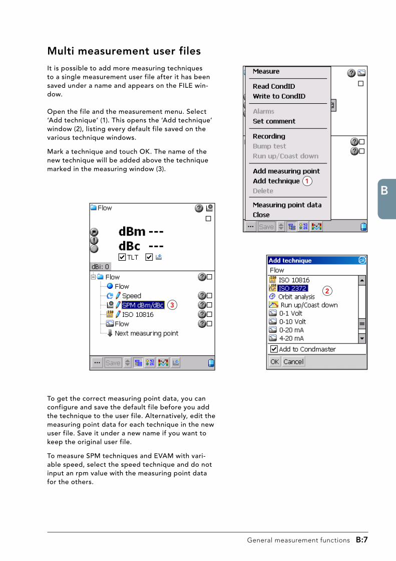
It is possible to add more measuring techniques to a single measurement user file after it has been saved under a name and appears on the FILE win-dow.
Open the file and the measurement menu. Select ‘Add technique’ (1). This opens the ‘Add technique’ window (2), listing every default file saved on the various technique windows.
Mark a technique and touch OK. The name of the new technique will be added above the technique marked in the measuring window (3).
Multi measurement user files
�
�
�
To get the correct measuring point data, you can configure and save the default file before you add the technique to the user file. Alternatively, edit the measuring point data for each technique in the new user file. Save it under a new name if you want to keep the original user file.
To measure SPM techniques and EVAM with vari-able speed, select the speed technique and do not input an rpm value with the measuring point data for the others.

B:� General measurement functions
B
‘Recording’ on the measurement menu (1) is a function for taking a stated number of readings at stated intervals, or measure for a stated number of minutes.
Default files and single measurement user files can be used when recording a single quantity, e. g. shock pulses or a certain type of vibration.
However, the strong feature of ‘Recording’ is con-secutive measurement of different quantities, using up to three different transducers simultaneously connected to Leonova:
• a shock pulse transducer on the SPM input.• one or two vibration transducers, alternatively an
analog signal on the VIB input.• a tachometer or temperature probe on the cen-
tre input.
To set up a consecutive recording of a shock pulse measurement, a vibration or analog measurement plus either a speed or temperature measurement (or any combination of these), one needs a measur-ing point where all wanted techniques are active. This point is either downloaded from Condmaster, or it is a multi measurement user file (see previous page).
Define the number of measurements or minutes (2) and the time interval (3) between measurements (0 minutes = as fast as possible). Use the key NEW (4) to select measuring techniques from the list (5) and put them into the measuring sequence (6). A select-ed technique can be replaced by another with EDIT (7) or be deleted with (8). Connect the transducer(s) and touch MEASURE to start.
The results can be seen on the graphics display and can be uploaded to Condmaster.
For SPM and EVAM measurements with variable speed, select ‘Speed’ as a technique and do not input an rpm under ‘Measuring point data’.
Recording
�
�
�
� 7 �
6
5

General measurement functions B:�
B
For efficient, systematic condition monitoring, Leonova is used as a data logger. Measuring points are set up in Condmaster and down-loaded to Leonova, complete with all input data for any or all of the supported measuring techniques. For instructions, see ‘Working with Condmaster Nova and the Leonova Instru-ments’, SPM 71805.
Downloaded measuring rounds are placed in the FILE window (1). To measure, mark the file and touch OPEN (2).
Measuring rounds cannot be renamed, be-cause Condmaster needs the original round name as an identifier.
After uploading, a measuring round can be deleted (3). If you keep it in Leonova, it will be overwritten next time you download the same round from the PC.
Measuring points in downloaded rounds are shown in round order, with the first measuring technique marked. All the operator has to do is to connect the appropriate transducer and use the Leonova keys MEAS and SAVE to obtain and save the measurements.
It is possible to add a technique to a measur-ing point (4). This technique will be automati-cally saved as part of the measuring point in Condmaster.
A new point can also be added to a measuring round (5). It is sufficient to name the point and to select at least one measuring technique. On uploading the round, the point can be properly named and numbered.
Please note that this new point will not remain in the round to which is was added. To make it a permanent part of the round, go to the round register and add it.
Measuring rounds from Condmaster
�
�
�
�
5
B:�0 General measurement functions
B
Measuring rounds for CondID
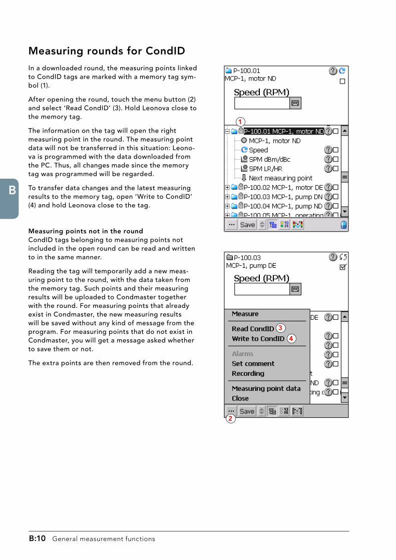
In a downloaded round, the measuring points linked to CondID tags are marked with a memory tag sym-bol (1).
After opening the round, touch the menu button (2) and select ‘Read CondID’ (3). Hold Leonova close to the memory tag.
The information on the tag will open the right measuring point in the round. The measuring point data will not be transferred in this situation: Leono-va is programmed with the data downloaded from the PC. Thus, all changes made since the memory tag was programmed will be regarded.
To transfer data changes and the latest measuring results to the memory tag, open ‘Write to CondID’ (4) and hold Leonova close to the tag.
Measuring points not in the roundCondID tags belonging to measuring points not included in the open round can be read and written to in the same manner.
Reading the tag will temporarily add a new meas-uring point to the round, with the data taken from the memory tag. Such points and their measuring results will be uploaded to Condmaster together with the round. For measuring points that already exist in Condmaster, the new measuring results will be saved without any kind of message from the program. For measuring points that do not exist in Condmaster, you will get a message asked whether to save them or not.
The extra points are then removed from the round.
�
�
�
�

General measurement functions B:��
B
The measuring sequence
Default files� Select a file (technique menu).
� Open the file. • Open ‘Measuring point data’. • Edit ‘Measuring point data’, all param-
eters. • Close ‘Measuring point data’.
� Connect the transducer.
� Press the MEAS key (or open the Measure menu and touch ‘Measure’).
• Repeat the measurement until satisfied. • Touch the Select button on the action
bar to leaf through the measuring results. • Set comment.
5 Press the SAVE key (or touch the ‘Save’ but-ton on the action bar, or press ENT when ‘Save’ is marked).
• Measure again.
6 Close the file with ‘Close’ on the Measure menu, or use ‘Save as’ to save it as a user/new default file.
Configured files� Select a file (FILE menu).
� Open the file.
� Connect the transducer.
� Press the MEAS key (or open the Measure menu and touch ‘Measure’).
• Repeat the measurement until satisfied. • Touch the Select button on the action
bar to leaf through the measuring re-sults.
• Set comment.
5 Press the SAVE key (or touch the ‘Save’ but-ton on the action bar, or press ENT when ‘Save’ is marked).
• Measure next item, measure again.
6 Close the file with ‘Close’ on the Measure menu, with or without saving.
Measuring with Leonova, especially data logging with downloaded, fully configured files, is very simple. While the file is open, only two keys are needed: MEAS and SAVE.
B:�� General measurement functions
B
Measurement window before measuring
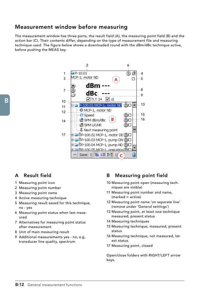
The measurement window has three parts, the result field (A), the measuring point field (B) and the action bar (C). Their contents differ, depending on the type of measurement file and measuring technique used. The figure below shows a downloaded round with the dBm/dBc technique active, before pushing the MEAS key.
A Result field1 Measuring point icon2 Measuring point number3 Measuring point name4 Active measuring technique5 Measuring result saved for this technique,
no - yes6 Measuring point status when last meas-
ured7 Alternatives for measuring point status
after measurement8 Unit of main measuring result9 Additional measurements yes - no, e.g.
transducer line quality, spectrum
B Measuring point field10 Measuring point open (measuring tech-
niques are visible)11 Measuring point number and name,
(marked = active)12 Measuring point name ‘on separate line’
(remove under ‘General settings’)13 Measuring point, at least one technique
measured, present status14 Measuring techniques15 Measuring technique, measured, present
status16 Measuring technique, not measured, lat-
est status.17 Measuring point, closed
Open/close folders with RIGHT/LEFT arrow keys.
13
7
10
11
5
12
17
14
2 6
13
1516
A
C
8
9
B
4

General measurement functions B:��
B
Measurement window before saving
The measurement is started by connecting the transducer and pushing the MEAS key.
The main result (1) is displayed in the measurement field and the status is shown by a larger status icon on top of the alternatives (2).
At this stage, the measuring result is not yet saved. The alternatives are to save it now or to repeat the measurement.
C Action barAll choices on the action bar are linked to the measuring point and technique selected in the meas-urement window shown here. 3 Opens the measurement window.4 Opens the measuring result window, which shows the whole list of results from the active meas-
urement. From version 2.xx, the values are displayed both before and after saving. The type of result(s) marked in that window is shown in the graphics window (7).
5 The ‘Select’ key. In case several measurements where taken, it is used before saving to leaf through the results. The selected results are shown in the result field (1), in the measuring result window under (4) and in the graphics window under (7).
6 Saves the results of the measurement shown in the result field (1). Erases all other measure-ments in case several were taken. Erases the values from the measuring result window under (4). Goes to the next item in the measurement window.
7 Graphics window showing a) the selected measurement taken before saving, or b) all down-loaded and saved measurements after saving, for the active measuring point and the result type selected under (4).
8 Spectrum display, if any.9 Measuring point data.
21
9 6 87435
C
B
A

B:�� General measurement functions
B
Comments
The option ‘Set comment’ (1) on the ‘Measuring point data’ menu is open for all types of measure-ments.
Comments consists of a ‘standard comment’ (2) and an optional free text (3) of up to four lines. The present date and time are set automatically in the field ‘From date/time’ (4). They can be edited.
In the graphics display, the comment appears as a square (colour coded in Condmaster) on the time line.
As an option, a future date and time can be input in the field ‘To date and time’. This changes the square on the time line of the graphics display into a bar that cover the time interval between the two dates and times.
The complete list of standard comments contained in Condmaster is downloaded with the measuring rounds and is available when data logging.
When measuring with the Leonova default files, you have four ‘Default comments’ (6) to which you can add free text. The text ‘Default comment’ can not be edited.
�
�
�
�
5
6

General measurement functions B:�5
B
The graphics window shows measuring results as dots (1) against a neutral scale or, in case of evaluated measuring results, a condition scale. Alarm limits set in Condmaster are marked by hori-zontal lines. The type of measuring result (2) is selected in the measuring result window.
Up to 100 measuring results can be downloaded with a measuring round from Condmaster. The setting is made under ‘Measuring system’ when Leonova is activated. Downloading 5 to 10 meas-uring results is quite sufficient to see the trend when the new reading is taken. The new result is shown before it is saved.
Graphics window
Touching a measuring result dot displays the measuring time and the values (3). Touch and hold displays the choice of deleting the result (4). Dragging the stylus into the diagram produces cross hairs. Dragging the stylus over part of the diagram (5) zooms in on the period. Dragging the stylus over the scale (6) changes the amplitude range. Comments are placed along the time line and open when touched (7, 8). Tap and hold on the comment line to add a new comment. Comments can be edited and deleted.
The functions on the Graphic menu are
9 ‘Zoom back’ reverts the last zoom step, while ‘Zoom back all’ returns to the original time span.10 ‘Measuring protocol’ spaces the measuring result dots evenly, regardless of the time intervals
between measurements.11 ‘Autoscale Y-axis’ sets the scale to the min. - max. range of the measuring results.
↑
↑
↑
�
�
�
�
5
6
7�
��
�0
�

B:�6 General measurement functions
B
The measuring result window is important for measuring techniques that return several values. The result field (1) can have max. three lines. The measuring technique SPM LR/HR returns five values. The EVAM method can produce many more, as even all symptom values are displayed. The scroll bar (2) indicates that there are more parameters than those visible on the screen.
The measuring result window also shows the units of measurement (3), if any.
The values of the marked parameter (4) are shown in the Graphics window (5).
Measuring result window
The measuring results are shown in this window both before and after saving the present meas-urement. An active ‘Select’ button (6) indicates that several readings have been taken, waiting for selection. All can be seen in this window when leafing through them with this button.
�
�
�
6
�
�
�
�
5

General measurement functions B:�7
B
The live spectrum window shows a continu-ously updated spectrum with 200 lines, ir-respective of other settings. The window will come up before measuring with the vibration measuring techniques and rotor balancing.
This function is activated under the TOOLS menu. Select ‘General settings’ and mark ‘Pre-view live spectrum’ (1).
‘Re-scale’ (2) will adjust the Y scale to fit the highest value and ‘Lock scale’ (3) will lock the Y scale.
Temporary settings can be made in the setting window, press the arrow button (4).
When pressing ‘Measure’ the pre-set assign-ment will be performed.
In the settings window (5), you can temporarly change upper frequency, spectrum unit, FFT type, average type and count.
Select parameter with the UP/DOWN buttons and change value with LEFT/RIGHT. Pre-set values for the measuring point are shown in blue, changed values in black. Changes will not affect settings made under ‘Measuring point data’.
Live spectrum window
�
�
�
�
5

B:�� General measurement functions
B
Spectrum window
The upper part of the Spectrum window shows the result field (A). Below that is the spectrum field (B) and at the bottom the Action bar (C).
The spectrum diagram is marked with the (displayed) range (1) in Hz, CPM or orders, depending on the setting under ‘General settings’.
The Y-axis (2) is marked with the measuring unit for spectrum line amplitude and with the range. To select the spectrum type unit, SD or SL, press the menu button (3) and select ‘Measuring point data’.
The button ‘...’ opens the spectrum menu (4). ‘Settings’ on the spectrum menu opens the symptom menu (5).
�
5
A
�
C
�
B
�

General measurement functions B:��
B
ZoomTo zoom in on the X-axis of the spectrum, place the stylus inside the diagram (1) and drag horizon-tally, in either direction. The dis-played range is shown below the diagram (2).
To zoom in on the Y-axis, drag vertically (3). The amplitude scale changes.
Cross hairsTo produce cross hairs that can be moved anywhere in the spectrum, place the stylus anywhere outside of the diagram (5), then drag it into the diagram. The position of the cross hair centre (6) along the X- and the Y-axis is displayed (7).
MarkerTo put a marker into the spectrum, point with the stylus anywhere inside of the diagram and keep it on the screen (‘tap and hold’) until a vertical ar-row appears (8). The arrow can be dragged with the stylus. For fine work, move the marker sideways with RIGHT/LEFT. One step corresponds to spectrum resolution (minimum distance between two spectrum lines).
At each step, the marker jumps to the top of the spectrum line or, if there is none, to the base line (amplitude = 0). Frequency and amplitude of the marker position are briefly displayed (9).
When the arrow coincides with a position belonging to a symptom, the name of the symptom is displayed (8). In case several symptoms share the same posi-tion, all relevant symptom names are displayed.
On the spectrum menu (4), you can undo the last zoom step with ‘Zoom back’ or restore the original diagram with ‘Zoom back all’.
Spectrum functions
Regarding display and available functions, there is no difference between a vibration spectrum and an SPM spectrum. The spectrum type is recognised from the measurement unit and the ampli-tude unit.
∆
∆
�
�
�
�
�5
7
6
�

B:�0 General measurement functions
B
The purpose of a spectrum is to reveal line patterns associated with machine or bearing faults. Characteristic for many fault patterns is the presence of ‘multiples’ or ‘harmonics’, which means that the line (or group of lines) is repeated two, three or more times further up in the spectrum. The spacing is 1Z, 2Z, 3Z, ... nZ, where Z = the frequency of the first line.
With the marker (1) on a line that has a significant amplitude, open the spectrum menu and select ‘Show harmonics’ (2).
The marker is replaced by a series of numbered broad arrows (3). Number 1 is in the marker posi-tion. Numbers 2, 3, etc. are the harmonics. They are evenly spaced along the frequency axis at Z inter-vals. Moving the marker one step and back will again display its position and thus Z.
To remove markings from the spectrum, use ‘Clear all (4) on the spectrum menu. The lower figure show the effect of placing the marker on the second large line in the pattern and again selecting ‘Show har-monics’. This line has one harmonic within the dis-played frequency range. Z is doubled.
Please note that Number 1 in the lower figure also matches the symptom ‘Bearing, BPFI’. This shows that the symptom is configured to look for multiples of the basic pattern. More about symp-toms overleaf.
Z
Z Z
�
Z
Z Z Z Z Z
� �
�

General measurement functions B:��
B
Spectrum functions on the ‘Settings menu’
The option ‘Settings’ on the spectrum menu opens a window with further functions for the spec-trum window:
1 Use logarithmic scales.
2 Recall saved or downloaded spectra.
3 Highlight a theoretical symptom in the spectrum.
4 Select a downloaded symptom.
‘Symptoms’ are instructions to search for and highlight spectrum lines or groups of spectrum lines that are typical for certain machine faults. Their purpose is to point out the significant data contained in the spec-trum.
Symptoms are selected and configured when the measuring point is created in Condmaster. They are downloaded with the measuring round. The only fac-tor added in Leonova is normally the machine speed (unless the measuring point is configured with a fixed rpm, which it should not be when spectra are meas-ured).
For an SPM spectrum, the list of symptoms shows the number of matches (5, 6), i. e. the spectrum lines with amplitudes above 0 that fit the calculated pattern. When the spectrum is measured with an appropriate resolution and over a frequency range large enough to accommodate the pattern, the number of matches will normally equal the number of lines in the symptom.
The two symptom marked in the figures both look for BPFI, the ball pass frequency over the inner race. The symptom (5) only looks for the line itself (1 possible match), while the symptom marked (6) looks for the same line plus three harmonics (4 possible matches).
6
�
�
�
�
5

B:�� General measurement functions
B
The effect of a logarithmic Y-scale is illustrated below, using a downloaded vibration spectrum.
The amplitude scale of a spectrum is automatically scaled to accommodate the largest spectrum line (1). Thus, a dominant line will make most others invisible, which is desirable, because the lines containing very little energy are insignificant for the evaluation of machine condition. In this exam-ple, the amplitude scale is marked 0 - 0.386 mm/s, so even the largest spectrum line is small.
5
��
�
�
Switching to a logarithmic scale amplifies the low amplitude values (2). The amplitude unit gets the ad-dition ‘LOG’ (3). This display form clearly shows that the FFT calculation produces spectrum lines in almost every position, most with amplitudes well below 0.002 mm/s.
The date above the scale (4) shows that the spectrum was saved in Leonova or downloaded from Cond-master. It was elected from the list under ‘Measuring results’.
For saved spectra, the measurement result is not shown in the result window (5). To see the result, go to the Graphics window and open the result for this date and time.
Please note: Saved spectra will be erased from the Spectrum window when ‘Clear all’ on the spec-trum menu is selected.

General measurement functions B:��
B
Highlighted symptoms in the spectrum
The following examples show different options on the ‘Settings’ menu and their effect on the spectrum display.
Theoretical symptom: Not marked.
Selection: No symptom.
A. Symptoms are not marked in the spectrum.
Theoretical symptom: Not marked.
Selection: Single line symptom.
B. The symptom name is shown (1). The symptom line is marked with a red dashed line (2) if a match is found in the spectrum. To find the match, Leonova searches for the closest peak line within the tolerances programmed in Condmaster.
Theoretical symptom: Marked
Selection: Single line symptom.
C. The symptom name is shown, plus the text ‘Theoretical symptom’ (3). The line in the calculated symptom position is marked with a blue dashed line (4). Leonova does not search for the closest peak.
A
B�
�
C�
�

B:�� General measurement functions
B
The previous page illustrated the three basic alternatives on the ‘Settings’ menu with single line symptoms. Here are examples of multi line symptoms:
Selection: Single line symptom with harmonics.
D. Same as B, but containing the line at BPFI plus three harmonics, altogether four possible match-es (5). In this example, the match found by Leonova agrees with the obvious peaks in the spec-trum: all dashed lines are on top of the largest lines (6).
D
Selection: Single line symptom with harmonics.
E. Same as C, marking the positions where BPFI and its three harmonics should be according to the calculations. In case of the first line (7), reality as reproduced by the FFT agrees with the cal-culation. However, the next three lines in the pattern are not quite in their calculated positions: they are beside the dashed lines (8).
Please note that such near misses are normal, es-pecially for the more rigid ‘Theoretical symptom’. Vibration itself is a continuous event, which is first digitalized during measurement and the subjected to mathematical manipulations to get the spectrum. At every step, there are tolerances, so an offset must be expected.
The resolution of this spectrum is 0.15625 Hz, so the line is offset by a single digital step.
5 6
E
�7
General measurement functions B:�5
B
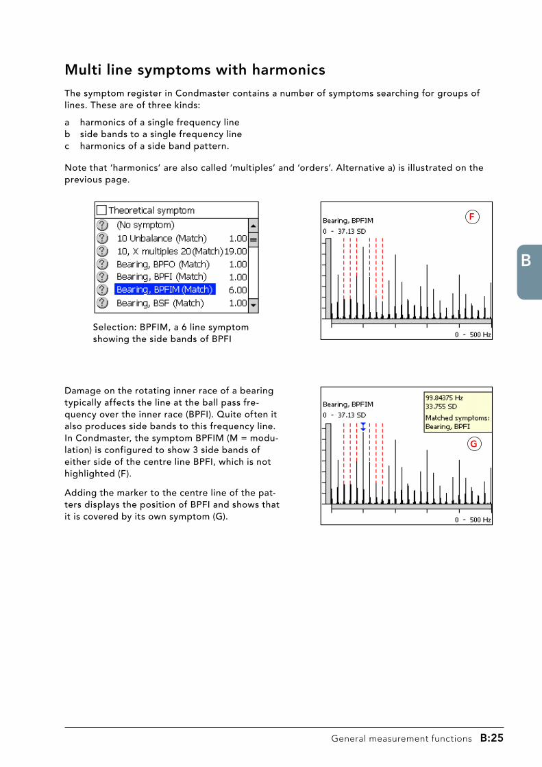
Multi line symptoms with harmonics
The symptom register in Condmaster contains a number of symptoms searching for groups of lines. These are of three kinds:
a harmonics of a single frequency lineb side bands to a single frequency linec harmonics of a side band pattern.
Note that ‘harmonics’ are also called ‘multiples’ and ‘orders’. Alternative a) is illustrated on the previous page.
Selection: BPFIM, a 6 line symptom showing the side bands of BPFI
Damage on the rotating inner race of a bearing typically affects the line at the ball pass fre-quency over the inner race (BPFI). Quite often it also produces side bands to this frequency line. In Condmaster, the symptom BPFIM (M = modu-lation) is configured to show 3 side bands of either side of the centre line BPFI, which is not highlighted (F).
Adding the marker to the centre line of the pat-ters displays the position of BPFI and shows that it is covered by its own symptom (G).
F
G

B:�6 General measurement functions
B
Harmonics of a side band pattern tend to put a lot of highlighters into the spectrum, which can be confusing. There is also a strong possibility that the multiples of the basic pattern overlap.
In the symptom shown below (H, I), the number of side bands has therefore been reduced to two on either side of the centre line.
Selection: BPFIM with 2 side bands of BPFI and 4 harmonics
The pattern in (H) is made clearer by placing marker on top of the BPFI line and selecting ‘Show harmonics’ on the spectrum menu (I).
Please note: While the presence of side bands and multiples in a spectrum is significant, the actual number of such elements is not important. The job of a symptom is to point out relevant data, not to find ‘everything’.
Zooming in on the spectrum (1) and sweeping a cluster of lines reveals, how close significant lines can be together.
The BPFI factor of this bearing is 4.919, so the har-monics of BPFI are spaced about five side bands apart. The symptom ‘Bearing, BPFIM’ looks for 3 side bands, while symptom ‘Bearing 4, BPFIM’ looks for four harmonics but only two side bands. In position (2), we see the third upper side band of the original BPFI. In position (3), we see the second lower side band of the harmonic.
H
I
�
��
�
H
Position (3) is a harmonic (order, multiple) of the fundamental frequency 1X. In this case we see 5X, which is of course close to BPFI (at 4.919X). In a low resolution spectrum, the three lines will be lumped together and shown as a single line.

General measurement functions B:�7
B
Waterfall diagram
�
The waterfall diagram is a three dimensional display of up to 99 vibration spectra. The dif-ferent readings are displayed along the Z coor-dinate, with the latest reading in the front.
To display a waterfall diagram, go to the spec-trum window (1). Under the ‘. . .’ button (2), go to ‘Settings’ (3) and select a number of dia-grams to show (4).
Hair cross and markers are only valid for the spectrum in the front. For the marker position in the spectrum, the frequency, amplitude and phase angle are shown.
Settings and other graphical functions are the same as for spectrum, see ‘Spectrum functions’ earlier in this part of the manual.
�
�
�

B:�� General measurement functions
B
Phase spectrum
If a time signal is measured together with a ta-chometer pulse a phase spectrum can be dis-played. This type of spectrum is useful especially when measuring on two channels.
To see a phase spectrum, go to the spectrum window and mark ‘Phase spectrum’ under the ‘. . .’ button (1).
Under ‘Settings’ you can mark ‘Show phase noice’ (3) to see the phase angle for each line included in the spectra.
Tap and hold to produce the blue marker (2). For the marker position in the spectra, frequency, am-plitude and phase angle are shown (4).
Move the blue marker with the right/left arrow keys.
All other settings and graphical functions are the same as for spectrum, see ‘Spectrum functions’ earlier in this part of the manual.
�
�
�

General measurement functions B:��
B
The time signal
The measuring unit (1) is always the signal unit, i. e. the transducer output. The diagram is scaled peak to peak (Y-axis) and shows the total sample time (2) along the X-axis.
Menu selected functions under (�) are:Zoom back: undo last zoom step.Zoom back all: show original spectrum.Show periods: when two markers are active, this shows all multiples of the time interval between the markers.Clear all: removes markers and other indicators, and even removes a time signal that was selected from the list of saved time signals.
Settings: opens a menu (4) where one can select another time signal if available.
The time signal can be saved for vibration measurement. It can be seen directly after measuring and before saving, or by calling up any stored measurement for the active measuring point (se-lected under settings).
�
�
�
�

B:�0 General measurement functions
B
To zoom in on a time range, drag the stylus hori-zontally over a part of the diagram (1).
To zoom in on a part of the amplitude scale, drag the stylus vertically over a part of the diagram (2).
To put cross-hairs into the diagram, drag the sty-lus from any point outside into the diagram (3). The time and amplitude of the cross-hair centre is displayed (4) as you move the cross-hairs with the stylus.
To put a marker (5) into the graph, point with the stylus and keep it on the screen (tap and hold) until a blue vertical arrow appears. The marker can be moved sideways with RIGHT/LEFT, and it can also be dragged with the stylus. At each step, the time and amplitude of the spot beneath the marker are briefly displayed.
A period is selected by placing a second marker (6). Hold down SHIFT, then tap and hold in the second marker position. The frequency for the period is shown in Hertz, together with delta values (7):
Delta time = time between the two markers
Delta amplitude = difference in amplitude between the two markers.
Delta phase = difference in phase angle between the two markers.
Note: Phase angle is shown only if rpm is mea-sured.
The RIGHT/LEFT buttons moves the first marker. SHIFT + RIGHT/LEFT moves the second marker. To mark a different period, use CLEAR ALL and start again.
The menu choice ‘Show period’ shows all multi-ples of the period between the two markers (8).
Pointing/dragging with the stylus opens more functions:
�
�
�
�
5
7
6
�

Free measurement techniques C:�
C
Free measurement techniques
ContentsFree measurement techniques .............................................. 3
Speed measurement ............................................................. 4
Speed measurement with default file .................................... 5
Temperature measurement ................................................... 6
Temperature measurement with default file .......................... 7
Analog measurement ............................................................ 8
Configuration of analog measurement file ............................ 9
Vibration severity measurement .......................................... 10
Definition of machine classes according to ISO 2372 ...........11
Measuring points for vibration ............................................ 12
Selection of vibration transducer ........................................ 13
Measuring point data for ISO 2372 ...................................... 14

C:� Free measurement techniques
BC
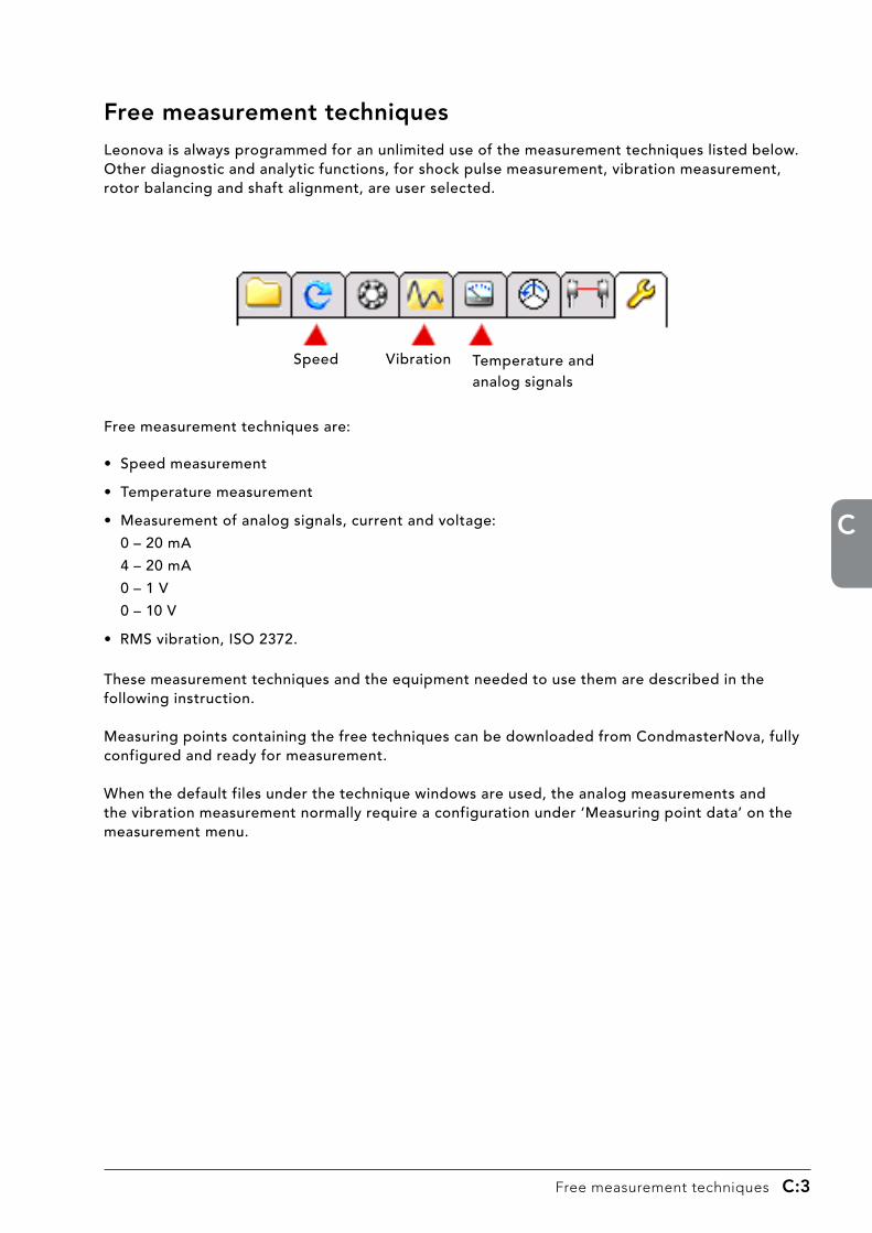
Free measurement techniques C:�
C
Free measurement techniques
Leonova is always programmed for an unlimited use of the measurement techniques listed below. Other diagnostic and analytic functions, for shock pulse measurement, vibration measurement, rotor balancing and shaft alignment, are user selected.
Temperature andanalog signals
Speed Vibration
Free measurement techniques are:
• Speed measurement
• Temperature measurement
• Measurement of analog signals, current and voltage:
0 – 20 mA
4 – 20 mA
0 – 1 V
0 – 10 V
• RMS vibration, ISO 2372.
These measurement techniques and the equipment needed to use them are described in the following instruction.
Measuring points containing the free techniques can be downloaded from CondmasterNova, fully configured and ready for measurement.
When the default files under the technique windows are used, the analog measurements and the vibration measurement normally require a configuration under ‘Measuring point data’ on the measurement menu.

C:� Free measurement techniques
BC
Speed measurement
RPM, optical:Distance max. 0.6 m (2 feet)
Reflectingtape
RPM, contact centre:Hold it against the shaft centre
Peripheral, contact wheelsMultiply the reading by the wheel factor:
TAD-12 0.1 m/min.TAD-13 0.1 yd./min.TAD-17 0.5 ft./min.
Input for tachometer probe
The SPM tachometer probe TAD-18 is used for both optical and contact speed measurement. It is connected to the middle transducer input.
TAD-18

Free measurement techniques C:�
C
Optical speed measurement
Easiest is the optical speed measurement. The preparations are simple: paste a bit of adhesive reflecting tape on the rotating part. It has to be reasonably clean.
Direct the light beam at the reflecting tape. Press MEAS key. A green LED shows that the light beam is on target. The count is displayed in a small window (2). When it stabilizes, touch ‘Continue’. Save the result or measure again.
The instrument counts 1 rpm for each received light reflex. The minimum is one count every 6 seconds (corresponding to 10 rpm). On slowly rotating parts you can use several reflexes at even intervals, and divide the displayed value by the number of tape bits to get the rpm.
Speed measurement with default file
Please note: to evaluate bearing condition and to make sense of a vibration spectrum, one has to know the rpm of the shaft. This type of rpm measurement is made as part of the shock pulse or vibration measurement, where the speed technique is automatically included when the point is config-ured for ‘variable speed’.
The speed measure with the default file is not avail-able for other measurements.
For the default file, there are no settings to be made under ‘Measuring point data’ (1). It is possible to change the speed unit from RPM to some other unit, but Leonova will always count the number of light reflexes.
Contact measurement
For contact measurement, you place the contact adapter over the lens and fix a contact centre or a wheel. The adapter has a reflecting tape inside, and each revolution sends one light reflex to the counter. The contact centre is pressed firmly into the cavity at the centre of the shaft, and the probe is aligned with the shaft’s centre line. The wheels are used to measure peripheral speed. One turn corresponds to 0.1 m, 0.1 yards, or 0.5 feet, depending on the wheel type. For meters or yards per minute, divide the displayed result by 10. For feet per minute, divide by 2.
�
�

C:� Free measurement techniques
BC
Temperature measurement
The temperature probe TEM-11 is used for temperature measurements in the range of –50 to +440 °C (–58 to +824 °F).
The probe TEM-11 is connected via the spiral cable CAB-10 to Leonova. It is power supplied by the instru-ment.
Two probe tips belong to TEM-11:
• TEN-10 for measuring the surface temperature of solids
• TEN-11 for measuring the temperatures of liquids.
Technical specifications
Measuring range: –50 to +440 °C(–58 to +824 °F)Maximum offset: ±5 °C (±9 °F)
TEN-��Probe tip for liquids
TEN-�0Probe tip for solids
TEM-��Temperature probe
CAB-�0Spiral cable
The probe tips fit into the socket at the front end of the probe. Probe and tips should be handled and stored with care. Keep the protective cap on the TEN-10 when the tip is not being used.
To measure, hold the probe tip TEN-10 against the object or dip TEN-11 into the liquid and press the MEAS key.
Measuring uncertainty: ± 1° CSensitivity: 10 mV / °COutput range: 0 to 5 V DCPower supply: +5 V DCMeasuring time: approx. 1 minute

Free measurement techniques C:�
C
Temperature measurement with default file
The default file for temperature measurements is located in the ANALOG window.
The result is displayed with a decimal, but please note that the accuracy of the SPM temperature probe is ± integer.
There are no settings under ‘Measuring point data’ (1).
The change from °C to °F is made under ‘General settings’ (2) in the TOOL window.
Switching from one unit to the other will re-cal-culate all saved results and display them in the active unit.
�
�
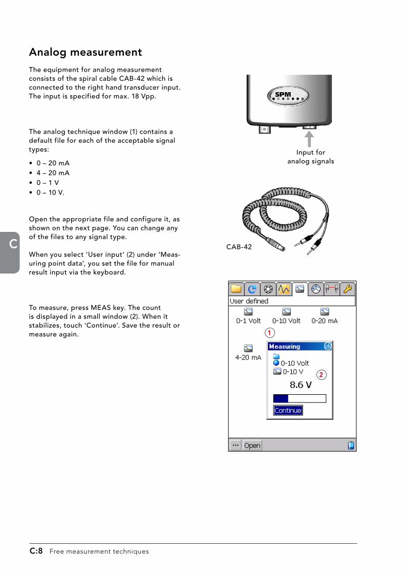
C:� Free measurement techniques
BC
Analog measurement
The equipment for analog measurement consists of the spiral cable CAB-42 which is connected to the right hand transducer input. The input is specified for max. 18 Vpp.
The analog technique window (1) contains a default file for each of the acceptable signal types:
• 0 – 20 mA• 4 – 20 mA• 0 – 1 V• 0 – 10 V.
Open the appropriate file and configure it, as shown on the next page. You can change any of the files to any signal type.
When you select ‘User input’ (2) under ‘Meas-uring point data’, you set the file for manual result input via the keyboard.
To measure, press MEAS key. The count is displayed in a small window (2). When it stabilizes, touch ‘Continue’. Save the result or measure again.
CAB-42
Input foranalog signals
�
�

Free measurement techniques C:�
C
� �
�
�
Configuration of analog measurement file
The default files for analog measurements have to be configured. Open ‘Measuring point data’ with the button (...).
‘Type’ is given when you select the appropriate file, e. g. ‘4-20 mA’, but can be changed to any of the other alternatives. It must, of course, correspond to the incoming signal. ‘Type’ is shown as the measur-ing point name in the measurement window (1).
‘Quantity’ is what the incoming signal represents, e. g. power, flow, pressure. The default setting is the name of the incoming signal. Mark this line and click the Edit button. Open the keyboard and write the new name. It will be displayed above the result field in the measurement window (2).
‘Unit’ is the measurement unit for the new quantity, here ‘bar’ for oil pressure. It is displayed in brackets above the result field (3).
‘Format’ defines the number of digits and the posi-tion of the decimal point in the result field (4). Write a ‘#’ for each digit.
Signal conversion
Correct signal conversion is the most impor-tant part of the configuration. Normally, you do not want to measure electricity but the quantity represented by the incoming signal.
‘Lowest value’ is the quantity represented by the lowest value of the incoming signal. In this example, the lowest incoming signal is 4 mA, and it represents here a value of 1.4 bar.
‘Highest value’ is the quantity represented by the highest value of the incoming signal, here 20 mA. In this example, this represents a value of 2.2 bar.
Thus, the measuring range is defined as 1.4 to 2.2 bar.

C:�0 Free measurement techniques
BC
Vibration severity measurement
Vibration severity measurement according to ISO 2372 is a broad band measurement over the frequency range 10 to 1000 Hz. It returns the RMS value of vibration velocity in mm/s (or inch/s). This value is representative of the energy contents of machine vibration, and thus of the destruc-tive forces acting on the machine. It is still widely regarded as a good and easy to obtain indicator of general machine condition.
Evaluation of machine condition
The evaluation consists of a comparison of the measured value with the ISO limit values recommended for 6 differ-ent classes (see definition on the next page).
The majority of industrial machinery belongs to the vibration classes 2, 3, and 4:
Class 2: Medium size machines without special foundations
Class 3: Large machines on rigid foun-dations
Class 4: Large machines on soft foun-dations.
For example, most smaller process pumps in a chemical plant would be Class 2. A 100 kW fan on a concrete foundation would be Class 3. However, the same fan fastened to the less rigid metal deck of a ship could be considered as Class 4.
Class 1 refers to independent parts of machines, for example electric motors up to 15 kW. Classes 5 and 6 are used for heavy reciprocating prime movers and machines which are intended to vi-brate, such as vibrating screens.
Leonova is programmed with the ISO limit values and will evaluate the measuring result, provided the ISO machine class number is input under ‘Measuring point data’. On the instrument, the ISO values for good and acceptable are shown as green. Just tolerable is yellow, unacceptable is red.
Class mm/sRMSLimits

Free measurement techniques C:��
C
Definition of machine classes according to ISO ����
The following text is a quotation from ISO 2372 (1974, E, page 6, Annex A). This ISO Recommenda-tion has also been published as British Standard (BS 4675, part I). A similar vibration classification of industrial machinery can be found in VDI 2056.
In order to show how the recommended method of classification may be applied, examples of specific classes of machines are given below. It should be emphasized, however, that they are sim-ply examples and it is recognized that other classifications are possible and may be substituted in accordance with the circumstances concerned. As and when circumstances permit, recommenda-tions for acceptable levels of vibration severity for particular types of machines will be prepared. At present, experience suggests that the following classes are appropriate for most applications.
Class IIndividual parts of engines and machines, integrally connected with the complete machine in its normal operating condition. (Production electrical motors of up to 15 kW are typical examples of machines in this category.)
Class IIMedium-sized machines, (typically electrical motors with 15 to 75 kW output) without special foundations, rigidly mounted engines or machines (up to 300 kW) on special foundations.
Class IIILarge prime movers and other large machines with rotating masses on rigid and heavy foundations which are relatively stiff in the direction of vibration measurement.
Class IVLarge prime movers and other large machines with rotating masses on foundations which are rela-tively soft in the direction of vibration measurement (for example turbogenerator sets, especially those with lightweight substructures).
Class VMachines and mechanical drive systems with unbalanceable inertia effects (due to reciprocating parts), mounted on foundations which are relatively stiff in the direction of vibration measurement.
Class VIMachines and mechanical drive systems with unbalanceable inertia effects (due to reciprocating parts), mounted on foundations which are relatively soft in the direction of vibration measure-ments; machines with rotating slackcoupled masses such as beater shafts in grinding mills; ma-chines, like centrifugal machines, with varying unbalances capable of operating as self-contained units without connecting components; vibrating screens, dynamic fatigue-testing machines and vibration exciters used in processing plants.

C:�� Free measurement techniques
BC
Measuring points for vibration
Vibration severity is primarily a measure for general machine condition. Vibration at the measuring point should be representative for the overall vibration of the machine.
Typical measuring points are the bearing housings. By measuring in three directions, one can get an indication of the causes for increased vibration.
• Horizontal vibration (H) in the plane of rotation is most representative of balance condition.
• Vertical vibration (V) in the plane of rotation is most representative of structural weakness.
• Axial vibration (A) along the line of the shaft is most representative of faulty alignment and bent shafts.
SPM vibration transducers can be used
• as a hand-held probe, with or without the probe tip attached. Not recommended above 1000 Hz.
• with a magnet for attachment to ferrous metal parts. Not recommended above 2000 Hz.
• with the M8 (UNC 1/4”-28) mounting screw.
The firmer the contact with the machine, the better the measuring result. Plain, clean metal makes the best contact surface for the vibration transducer.
To get comparable results, the measuring points should be clearly marked, so that the measurements can always be taken in the same spots.
Hand-held probe
Transducer with magnet

Free measurement techniques C:��
C
Selection of vibration transducer
The ‘Registration of vibration transducers’ is described in Part A of this manual. Before starting vibration measurements, make sure that the vibra-tion transducer you are using with your Leonova is properly registered, configured and selected.
The nominal sensitivity of a vibration transducer SLD144 is 10.0 mV/m/s2. The actual sensitivity of the individual transducer is written on its calibra-tion card. This data should always be input in the transducer register (1). When several transducers are in use, they should be marked to assure that the readings are calibrated.
To select a transducer, open ‘Vibration transducers’ in the TOOLS window. Mark its name on the list (2) and touch the arrow key (3). To see or edit its data, mark its name on the list (2) and touch the edit key (4).
�
�
��

C:�� Free measurement techniques
BC
Measuring point data for ISO ����
The only measuring point data that should be edited are ‘Direction’ and ‘Class’ (1). For both, the alternatives are selected from lists after marking the line and touching ‘Edit’ (2).
‘Portable’ on the transducer line (3) means that the transducer which is marked in the register is active. Its data are shown below. They should not be edited. If you are using a different transducer, you should register and select it as described on the previous page.
The selected measuring direction appears as measuring point name in the measurement win-dow (4).
To measure, connect the transducer and press MEAS. The selected machine class effects the evaluation of the measuring result (5).
�
�
�
�
�
�

Shock pulse measurement D:�
D
Shock pulse measurement
ContentsShock pulse techniques ......................................................... 3
Rules for SPM measuring points ............................................ 4
Examples of SPM measuring points ....................................... 6
Equipment for shock pulse measurement ............................. 8
Transducer with quick connector ........................................... 9
Permanently installed transducers/terminal ....................... 10
Shock pulse transducer with probe ......................................11
The dBm/dBc technique ...................................................... 12
Normalized condition readings ........................................... 13
Input data for SPM dBm/dBc ............................................... 14
Measuring SPM dBm/dBc .................................................... 16
Using the earphones ............................................................ 17
The LR/HR technique ........................................................... 18
Input data for SPM LR/HR ................................................... 19
Accumulation and compensation ......................................... 20
LR/HR values and CODE ...................................................... 21
The LUB number .................................................................. 22
The COND number and error codes .................................... 23
Input data for SPM LR/HR ................................................... 24
Measuring SPM LR/HR ......................................................... 26
Measuring an SPM Spectrum ............................................... 27
Editing the spectrum data ................................................... 28

D
D:� Shock pulse measurement

Shock pulse measurement D:�
D
Shock pulse techniques
The Shock Pulse Method for bearing condition monitoring (SPM) is applied as three related and complementary measuring techniques:
SPM dBm/dBc
Shock pulse magnitude is quantified on a decibel scale by two values, the maximum value dBm and the carpet value dBc. The input data are very simple: the rpm and the bear-ing’s shaft diameter. The maximum value dBm is evaluated on a green - yellow - red condition scale. It indicates the bearing’s operating conditions in terms of good - caution - bad. Operating condition includes factors like installation quality, load, lubrication and the mechanical state of the bearing surfaces.
SPM LR/HR
Shock pulse magnitude is quantified on a decibel scale by the values LR (low rate of occurrence, corresponding to the dBm) and HR (high rate of occurrence, corresponding to the dBc). In addition to these ‘raw values’, the bearing’s operating condition is indicated by the evaluation results CODE (overall condition), LUB (oil film thickness) and COND (mechanical state of the surfaces). Thus, condition informa-tion is more detailed, with emphasis on bearing lubrication.
The required input data are also more detailed: the rpm, the bearing’s mean diameter and its type number. The type number defines the bearing geometry and thus the evaluation box with its green - yellow - red condition zones.
For both techniques, measuring results indicating bad bearing condition should be verified. By comparing shock values on and around the bearing housing and by lubrication tests the operator can make sure that the measured shock pulses originate from the bearing before taking corrective action. This verification process is greatly simplified by the latest technique, SPM Spectrum.
SPM Spectrum
A time record of the shock signal is subjected to an FFT. Prominent bearing patterns in the resulting spectrum are conclusive evidence that the measured shocks are generated by the bearing. Thus, the bearing condition data obtained with either the dBm/dBc or the LR/HR method are valid.
TYPE 3
dBm
dBc

D
D:� Shock pulse measurement
� – In the load zone of the bearing
Rules for SPM measuring points
The rules for the selection of SPM measuring points have a very practical purpose.
We are trying to catch low energy signals which are getting weaker the farther they travel and the more they are bounced about inside a piece of metal.
We know that they lose strength when they cross over from one piece of metal to another (oil between the pieces reduces signal losses).
We cannot know, for all bearing applications, how much of the strength of the bearing signal will reach the measuring point.
However, of necessity we try to apply general evaluation rules, i. e. treat all measured signals as if they were of the same quality.
The rules for SPM measuring points try to assure that most signals are comparable, with sufficient accuracy, and that the green-yellow-red condition zones are valid.
� The signal path between bearing and measuring point shall be as short and straight as possible.
� The signal path must contain only one mechanical interface, that between bearing and bearing housing.
� The measuring point shall be located in the load zone of the bearing.
Measuring
point
Load
� – Straight and short path
� – No interface!

Shock pulse measurement D:�
D
Measuring points should be located directly on the bearing housing, i. e. the metal that is touching the outer race.
SPM supplies long adapters and transducers that allow you to reach measuring points beneath covers, shields and brackets.
The signal losses in the two unavoidable interfaces (bearing – bearing housing and housing – adapter) have been taken into account in SPM’s evaluation of bearing condition.
The load zone is defined as the load carrying part of the bearing housing. It is normally determined by the weight of the supported machine part, i.e. the load is mostly on the lower half of the bearing housing.
Consider also the direction of the force acting on the shaft when the machine is running. Thus, belt tension can determine the load on the bearings. The fan shaft in point 3 is pulled down towards the motor. The drive end of the motor shaft is pulled up towards the fan (2), the non-drive end (1) is pressed down and away from the fan. In point 4 the weight of the rotor normally determines the measuring direction. The arrows show the measuring points, numbered in the direction of power transmission.
Find the strongest signal
Use the shock pulse transducer with probe to find the spot on the bearing housing where the signal is strongest. If there are several points yielding the same signal, select the point where it is easiest to take readings.
When a measuring point cannot conform to the rules (because an ideal spot cannot be reached), make allowance for a weaker signal. If you use SPM LR/HR, you have a COMP no. to compensate for weak signals, but must still try to find a good point.

D
D:� Shock pulse measurement
The following pages show measuring points and possible adapter or transducer installations. How to install measuring equipment is described in the SPM installation manual.
Through hole for long adapter
A measuring point beneath a fan cover (1) can be reached with a long adapter, through a hole in the cover.
Adapter with lock nut
The fan cover is fastened directly to the motor shield, which is also the bearing housing (2). One of the cover’s holding screws can be replaced by an adapter with lock nut.
Bearing housings beneath brackets
Consult machine drawings and identify the bearing housing before selecting a measuring point.
In a pump, the bearings can be placed in two sepa-rate housings inside the bearing bracket (3).
Measuring point B, placed below and opposite to the pump outlet (because of the load direction) can be reached with a long adapter through an opening in the pump shield.
The bearing pair at measuring point A can be reached with a long adapter through a clearance hole in the bracket. The hole must be large enough to allow bearing adjustment and still prevent metallic contact between bracket and adapter.
Examples of SPM measuring points
�
�
B
�
A

Shock pulse measurement D:�
D
Multiple bearings in one housing
If there are several bearings in the same housing, they are normally treated as a single bearing. In the bearing arrangement for a vertical pump (4), it is not possible to distinguish between the shock pulses from the paired bearings in point 1.
There is also a risk for cross talk between point 1 and point 2, which means that the shock pulses from the bearing in worst condition are picked up in both points.
Check signal strength with the probe. Use one measuring point only if readings are identical in both points. This point (x) can be placed halfway between points 1 and 2.
Installed transducer
On large electric motors (5), the bearings are often mounted in bushings which are welded or bolted to the motor shields. Because of the damping in the interface between the bushing and the shield, the measuring point should be on the bushing.
The bearing bushing at the drive end (A) is usually within reach. A long adapter is installed at an angle to the shield, so that there is enough space for connecting the transducer.
The bearing at the fan end (B) requires a perma-nent transducer installation. The transducer is installed in the bushing. The coaxial cable is run through a slit in the fan cover to a measuring terminal on the stator frame.
�
X
�
�
A B
�
A. Drive end
B. Fan end

D
D:� Shock pulse measurement
CAB36
Measuring cable, BNC slip-on, 1.5 m
Equipment for shock pulse measurement
TRA72
Shock pulse transducer with probe
TRA70
Shock pulse transducer with quick connector
Hand-held transducers
Two types of hand-held transducers are available for shock pulse measurement with Leonova:
• Shock pulse transducer with quick connector, TRA70, for use with permanently installed measuring adapters.
• Shock pulse transducer with probe, TRA72.
Permanently installed transducers
Permanent installed transducers can be used in narrow spaces or when the bearing cannot be reached directly. The transducer is connected to a measuring terminal via a coaxial cable. Connect Leonova to the measuring terminal with a slip-on measuring cable.
• Standard transducer, type 40000, for cable length up to 4 m.
• Transducer with TMU, type 42000, for cable length up to 100 m.
• Measuring cable, CAB36, BNC slip-on, 1.5 m.
Transducers and measuring cables are connected to Leonova’s left hand input.
Note: For measurements with low dBi (low rpm or small bearings) the quick connector or permanently installed transducer is recommended.
Earphones
The earphones allows you to listen on the shock pulse pattern and is helpful for verifying and tracing the shock pulse sources. Two types of earphones are available.
• Earphone in ear defenders, EAR10, headset, with cable.
• Earphone in ear defenders for helmet, EAR11, with cable.
Earphones are connected to Leonova’s input/output connector in the middle.
EAR10
Earphone with cable
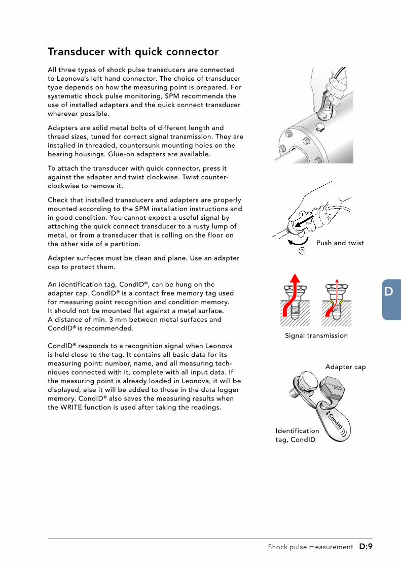
Shock pulse measurement D:�
D
Transducer with quick connector
All three types of shock pulse transducers are connected to Leonova’s left hand connector. The choice of transducer type depends on how the measuring point is prepared. For systematic shock pulse monitoring, SPM recommends the use of installed adapters and the quick connect transducer wherever possible.
Adapters are solid metal bolts of different length and thread sizes, tuned for correct signal transmission. They are installed in threaded, countersunk mounting holes on the bearing housings. Glue-on adapters are available.
To attach the transducer with quick connector, press it against the adapter and twist clockwise. Twist counter-clockwise to remove it.
Check that installed transducers and adapters are properly mounted according to the SPM installation instructions and in good condition. You cannot expect a useful signal by attaching the quick connect transducer to a rusty lump of metal, or from a transducer that is rolling on the floor on the other side of a partition.
Adapter surfaces must be clean and plane. Use an adapter cap to protect them.
An identification tag, CondID®, can be hung on the adapter cap. CondID® is a contact free memory tag used for measuring point recognition and condition memory. It should not be mounted flat against a metal surface. A distance of min. 3 mm between metal surfaces and CondID® is recommended.
CondID® responds to a recognition signal when Leonova is held close to the tag. It contains all basic data for its measuring point: number, name, and all measuring tech-niques connected with it, complete with all input data. If the measuring point is already loaded in Leonova, it will be displayed, else it will be added to those in the data logger memory. CondID® also saves the measuring results when the WRITE function is used after taking the readings.
Push and twist
Signal transmission
Adapter cap
Identification tag, CondID

D
D:�0 Shock pulse measurement
Permanently installed transducers/terminal
Installed transducer, cable to terminal
Measuringterminal
Input forshock pulse transducer
A permanently installed transducer and a measuring terminal (BNC or TNC connector) are used when the bearing cannot be reached directly. Use a measuring cable to connect Leonova to the terminal.
The terminal cabinet, SPM 14318, can receive up to 16 coaxial cables from shock pulse and vibration transducers. The cabinet is made of stainless steel and has protection class IP66.
Transducers for permanent installation are available with different thread sizes and in two types, series 40000 for cable length max. 4 m and series 42000 for cable length max. 100 m. They are installed in threaded, countersunk mounting holes on the bearing housings. The coaxial cable between transducer and terminal should be firmly attached to the machine with cable clamps and, where necessary, be protected against damage.
SPM supplies high temperature cables and moisture proof connectors.

Shock pulse measurement D:��
D
The hand-held probe is mainly used to locate the strongest shock signal on and around the bearing housing, in order to find the best measuring point or to verify the shock pulse source after getting a measuring result which indicates bad bearing condi-tion.
If it is used for regular condition monitoring, the measuring points for the hand-held probe should be clearly marked. Always measure in the same spot.
The probe tip is spring loaded and moves within a sleeve of hard rubber. To maintain a steady pressure on the tip, press the probe tip against the meas-uring point until the rubber sleeve is in contact with the surface.
Hold the probe steady to avoid rubbing between probe tip and surface.
The probe is directionally sensitive. It has to be pointed straight at the bearing.
The centre of the probe tip should touch the surface. Avoid pressing the probe tip against cavi-ties and fillets which are smaller than the probe tip.
The only part likely to wear out is the rubber sleeve for the probe tip. It is made of chloroprene rubber (neoprene) and tolerates 110° C (230° F). Spare sleeves have the part number 13108.
Rubber sleevein contact withthe surface
Point at thebearing
Hold steady
SPM 13108Neoprene, 110° C (230° F)
Shock pulse transducer with probe
Avoid smallcavities andfillets

D
D:�� Shock pulse measurement
The dBm/dBc technique has been successfully applied for more than 35 years and continues to be widely used. It is well suited for industrial condition monitoring, because it works with few, easy to understand in- and output data and with ‘reasonable accuracy’.
Even on a logarithmic scale, there is normally a large, distinct difference between the maximum values from good and bad bearings. Thus, minor inaccuracies in the input data (rpm and shaft diameter) have little effect on the evaluated measuring result.
Lubrication condition is indicated by the delta value, i.e. the difference between dBm and dBc. High readings and a small delta value indicate poor lubrication or dry running. This is sufficient for maintenance purposes.
dBm and dBc are measured in a fixed time window and automatically displayed. After that, the instrument continues to measure while the transducer is connected. The peak indicator blinks when pulses stronger than the displayed level are detected.
The earphone is used to listen to the shock pulse pattern in case of suspect or high readings. This, and the possibility to search for shock pulse sources with the probe transducer, is a means to verify the measuring result and its cause.
The dBm/dBc technique
RPM
Life time
d
dBm
dBcdBm dBc
dBm
dBc

Shock pulse measurement D:��
D
dBi = Initial value of a bearingdBc = Carpet value (weak pulses)dBm = Maximum value (strong pulses)dBn = Unit for normalized shock leveldBsv = Unit for absolute shock level
The absolute shock pulse level of a bearing, measured in dBsv (decibel shock value), is both a function of rolling velocity and of bearing condition. To neutralize the effect of rolling velocity on the measured value, Leonova has to be programmed with shaft diameter (in millimetre or inch) and rotational speed (in rpm).
The instrument will then calculate the initial value dBi, the starting point of the condition scale for a particular bearing. The dBi can also be input directly or via the ISO bearing number. The condi-tion scale is graded in normalized shock values, dBn.
Leonova samples the shock pulse amplitude over a period of time and displays:
• the maximum value dBm for the small number of strong shock pulses.• the carpet value dBc for the large number of weaker shock pulses.• the status dot which is green for dBm up to 20 dBn = good condition, yellow for 21-34 dBn =
caution, red for 35 dBn and more = bad condition.
The maximum value dBm defines the bearing’s position on the condition scale. The difference between dBm and dBc is used for a finer analysis of the causes for reduced or bad condition.
When you set the dBi to ‘0’, Leonova will take an unnormalized reading in dBsv (absolute shock values). The condition zones do not apply. This method is used for comparative reading on different bearings and/or other shock pulse sources.
Normalized condition readings
Absolute scale
(shock value)
Normalized scale
(condition)

D
D:�� Shock pulse measurement
For a normalized reading of bearing condition with the Leonova default file, it is necessary to edit the ‘Measuring point data’ and set the initial value dBi. The default setting is dBi = 0, which produces the unnormalized shock values without condition status display.
If known, the dBi can be input directly via the keyboard. Mark the line, then open it with the EDIT button (1).
Given the rotational speed (rpm) and the shaft diameter, Leonova will calculate and display the dBi.
There are two alternatives for shaft diameter. ‘Input ISO bearing number’ (2) opens a window (3) where you set the last two digits of the ISO number with the UP/DOWN keys on the Leonova key pad.
‘Input diameter’ (4) opens the keyboard (5). Write the shaft diameter, then edit RPM and write the rpm on the keyboard.
The dBi will be displayed when the data input is complete (6).
Input data for SPM dBm/dBc
�
�
�
�
�
�

Shock pulse measurement D:��
D
Variable speed
The alternative ‘Variable speed’ (7) implies that the shock pulse measurement is preceded by a measurement of the rpm. Ignore the message ‘RPM missing’. The dBi will be shown in the measurement window after the speed measure-ment.
Force new RPM reading
‘Force new RPM reading’ (8) is normally not used. With this setting on, you are forced to first measure the rpm again before you can repeat the shock pulse measurement.
TLT test
A last setting is made in the measurement window, by marking the TLT box (9) or not.
When TLT is on, the instrument will display the result of a transducer line test in the result window, so you can check the quality of signal transmission between transducer and instru-ment.
The TLT test should always be made when you measure with permanently installed transducers. Normal TLT values are around 20. TLT values below 15 are not acceptable, so you have to check cables and connectors for bad connec-tions and moisture. Part of your signal will be lost in a poor transducer line, so your measuring results are lower than they should be.
Measurement window, pre-set speed
Measurement window, variable speed
�
�
�
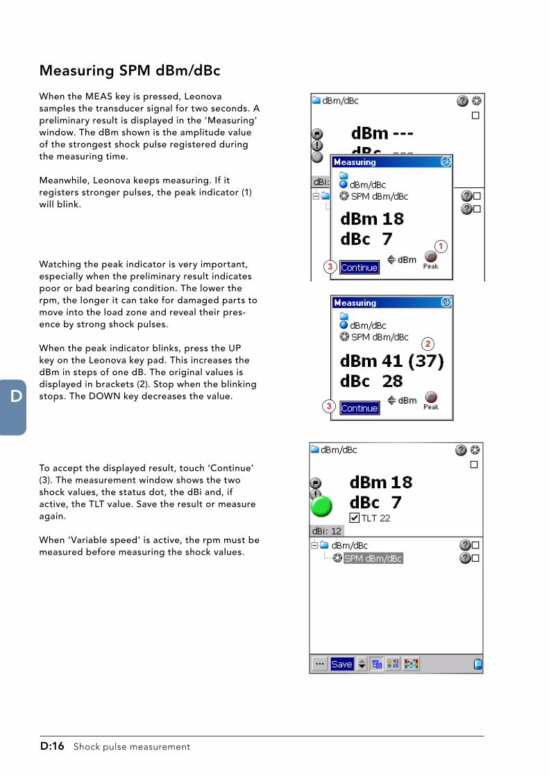
D
D:�� Shock pulse measurement
Measuring SPM dBm/dBc
When the MEAS key is pressed, Leonova samples the transducer signal for two seconds. A preliminary result is displayed in the ‘Measuring’ window. The dBm shown is the amplitude value of the strongest shock pulse registered during the measuring time.
Meanwhile, Leonova keeps measuring. If it registers stronger pulses, the peak indicator (1) will blink.
Watching the peak indicator is very important, especially when the preliminary result indicates poor or bad bearing condition. The lower the rpm, the longer it can take for damaged parts to move into the load zone and reveal their pres-ence by strong shock pulses.
When the peak indicator blinks, press the UP key on the Leonova key pad. This increases the dBm in steps of one dB. The original values is displayed in brackets (2). Stop when the blinking stops. The DOWN key decreases the value.
To accept the displayed result, touch ‘Continue’ (3). The measurement window shows the two shock values, the status dot, the dBi and, if active, the TLT value. Save the result or measure again.
When ‘Variable speed’ is active, the rpm must be measured before measuring the shock values.
�
�
�
�

Shock pulse measurement D:��
D
Using the earphones
The earphones allow you to listen to the shock pulse signal, which can help to pinpoint the cause for high values. Earphone listening does not work with the LR/HR technique.
The measuring threshold is change with the UP/DOWN keys on the Leonova key pad. At a low level, Leonova will emit a continuous tone. As the threshold is raised, this changes to very rapid pulses at the dBc level. At the dBm level, only a few pulses should occur at irregular intervals.
Significant are
• the dBm level• the rhythm of the pulses immediately below the dBm level• the delta value, which is the difference between the dBm and the dBc.
Shock pulses from a bearing normally occur at irregular interval, while strong, rhythmic shocks are a sign of disturbance. The diagrams below show typical patterns.
B
A. Good bearingShock values are low.
C
E F
D
B. Bad bearingHigh values, large delta,irregular pattern.
C. Pump cavitationVery small delta, fairly high shock level.
F. Measured value drops sharplyA danger signal, the bearing is sliding.
E. Regular showersScraping machine parts.
D. Load shocks, valves, etc.Regular patterns mean often disturbance
A

D
D:�� Shock pulse measurement
The LR/HR technique was originally developed for a continuous, automatic monitoring system (CMS). An automatic system can not, like a human operator, vary measuring time, use earphones or make ”further tests” to verify suspect readings. It works with fixed settings and is dependent on accurate input data. This, together with new research results, programmable chips, and the desire to get more detailed information from the shock pulse signal, lead to a change in the threshold values, plus a more diverse and detailed output.
The value for the noise carpet (HR) is read at an occurrence rate of approx. 1000 pulses/second, the value for the strong shock pulses (LR) at approx. 40 pulses/second. This makes LR an average value of the strong pulses, lower than the maximum, and thus reduces the dynamic range. To increase accuracy, the mean diameter of the bearing is used, the SPM TYPE no. is input to define bearing geometry, and the COMP no. to calibrate the individual measuring points.
The extra output information concerns mainly lubrication condition, allowing the user to attack a mayor maintenance problem (most bearings fail too soon because of inadequate lubrication) at the root. With SPM’s LUBMASTER® (part of Condmaster®Pro versions for this technique) and LR/HR readings, it is possible to accurately measure lubrication condition, calculate the resulting L10a life, and work out feasible improvements by simulating changes in the lubricant parameters.
The LR/HR technique
Mean diameter Dm
TYPE
RPM
COMP
TYPE 3 TYPE 1
LR HR

Shock pulse measurement D:��
D
One part of the input data, the rpm and the size of the bearing, is needed to allow for the effect of bearing speed on the shock level when evaluating bearing condition. The mean diameter Dm is more exact than the shaft diameter, because the height of bearings with the same shaft diameter can vary considerably. Together, rpm and Dm are used to calculate the NORM no. of the bearing (range 10 to 58).
The HR level shock pulses vary with the shape and number of the rolling elements in the bearing. This becomes important when estimating the oil film thickness in the rolling interface. The largest influencing factor is the shape of the contact area. In ball bearings, the rolling element has point contact with the raceways. In roller bearings, there is line contact, which means that the area under pressure, where the shock pulses occur, is much larger.
For SPM purposes, bearings are grouped into 8 different types, each with a TYPE number 1 through 8. The types are described in the table above.
Bearing manufacturers, though not all, follow ISO standards when numbering their bearings. The number code contains the information on mean diameter and bearing type. Thus, when you use an ISO bearing number as input in Condmaster®Pro, the program will give you Dm and TYPE no. As manual input for Leonova, you can use the last three digits of the ISO number, which will produce Dm but not the TYPE no.
Input data for SPM LR/HR
1 Deep groove ball bearings, series 62, 63, 64
2 Angular contact bearings, all series
3 Deep groove ball series 60, 160, 618, double row and self-aligning ball bearings
4 Thrust ball bearings, all types
5 Cylindrical roller bearings, single row
6 Taper roller bearings, all radial types
7 Spherical roller bearings Double row cylindrical roller bearings
8 Thrust roller bearings

D
D:�0 Shock pulse measurement
In addition to the basic input data, one can set values for COMP and ACCUM.
ACCUM (accumulation) determines the number of measuring cycles before the Leonova displays the average value as result. ACCUM can be set from 1 to 9. Especially on bearings with a low rpm, set ACCUM to at least 3.
COMP (compensation number) is used to calibrate the measuring point, normally to compensate for a somewhat weaker signal from a measuring point that does not quite comply with the SPM rules. To find the correct COMP no., use the LUBMASTER function in Condmaster®Pro.
A normal signal from a good bearing should be near the centre of the green part of the evaluation frame. If it is far to the left, you can ”push it forward” by setting a COMP no. If the signal is outside of the left side of evaluation frame, Leonova will display the error code E3 = signal too low. The COMP no. is added to the measuring result before it is evaluated. Thus, it will influence the evaluation results CODE, LUB, and COND, but not the displayed values for HR and LR.
It is possible to set negative COMP nos., but you should avoid that. With a positive COMP no., you make the evaluation results worse than apparent from the measured LR/HR values. With a negative COND. no., you ‘improve’ bearing condition, which can have unpleasant consequences if you are wrong in assuming that the signal from this bearing is stronger than normal. To avoid alarm from a stable bearing with high readings, it is better to change the alarm levels.
PositiveCOMP
Accumulation and compensation
NegativeCOMP

Shock pulse measurement D:��
D
For LR/HR values, the measuring unit is dBsv, i.e. these values are measured on the absolute shock pulse scale and do not, by themselves, express operating condition.
The term delta value simply means the difference between LR and HR.
The operating condition of the bearing is expressed by the CODE letter, the LUB no., and the COND. no., all of them not measuring but evalua-tion results.
CODE A means that the bearing is in good condition. There is no detectable damage to the surfaces of the load carrying parts, and no extreme lack of lubricant in the rolling interface.
CODE B indicates dry running. The lubricant is not reaching the rolling interface. This can have several causes, e.g. lack of lubricant supply to the bearing, low temperature in a grease lubricated bearing, or a heavy overload due to misalignment, tight fit, deformed housing, etc.
CODE C is displayed when the instrument detects an increased shock pulse level with a large delta value. This points to beginning surface damage.
CODE D is displayed when the signal is typical for bearing damage: a high shock level with a large delta value. Contamination of the lubricant by hard particles causes a similar signal.
The message of the codes is supported by the status dot: green for CODE A, yellow for B and C, red for D.
LR Measured value for strong shock pulses.
HR Measured value for weak shock pulses.
LR-HR Delta value.dBsv Unit for absolute shock pulse
value.
CODE A Good condition CODE B Caution, dry runningCODE C Caution, damage developingCODE D Bad condition
LR/HR values and CODE
B
CC
A
D
D

D
D:�� Shock pulse measurement
The most important influence on the service life of a bearing is the lubricant film between the load carrying rolling elements and the raceway.
By preventing or inhibiting metallic contact between the loaded bearing parts, the lubricant film reduces the local peak stress in the rolling interface. The greater the lubricant film thickness, the more even the load distribution in the contact area, and the better the fatigue life of the bearing.
Fulllubrication
Boundarylubrication
LUB Ball bearing
0 Dry running
1 to 2 Boundary
lubrication
3 to 4 Full lubrication
LUB Roller bearing
0 Dry running
1 to 4 Boundary
lubrication
> 4 Full lubrication
The LUB number
Irregularities in the bearing surfaces will always cause pres-sure variations in the contact area, and thus shock pulses, even when metallic contact is prevented by a separating lubricant film. A thinner film will result in an increase of the bearing’s HR value.
The LUB No., displayed with CODE A and B, is directly proportional to oil film thickness. LUB No. 0 means dry running condition. The interpretation of LUB Nos. between 1 and 4 depends on the bearing type. For ball bearings, LUB Nos. greater than 2 mean full lubrication (a load carrying oil film). For roller bearings, a LUB No. greater than 4 indicates full lubrication.
The term boundary lubrication implies that part of the load is carried by metal to metal contact. The amount of lubricant in or supplied to the bearing is only one of the many factors that deter-mine lubricant film thickness. Lubricant type and the bearing’s rpm are of great importance, but also the geometry of bearing parts and housing, as well as the load put on the bearing by align-ment and fitting.

Shock pulse measurement D:��
D
The COND number and error codes
CODE CCOND 28 to 32Beginning bearing damage
HR
LR
CODE CCOND >32Minor to severe bearing damage
HR
LR
The COND No. (condition number) is displayed with CODE B, C, and D, i.e. for all bearings with reduced or bad condition. It indicates the degree of surface deterio-ration or damage in the rolling interface.
Large (visible) surface damage typically leads to a very marked increase in the bearing’s LR readings and a high delta value. Thus, it is easily detected and will give Code D and high COND numbers.
When a COND number is displayed, the bearing should be watched very carefully. Once damage has started, it cannot be reversed. Temporary improvements of the COND No. only mean that the edges of fresh spallings or imprints have been rounded off. Soon, there will be new spallings. The time left to plan a bearing replacement depends on the trend of the COND No. As a rule, COND Nos. should be interpreted as follows:
COND No. < 30 Minor damage
COND No. 30 to 40 Increasing damage
COND No. > 40 Severe damage
ERROR CODES
E2 Disturbance
E3 Signal too low
When the measured signal is not within the evaluation frame, the Leonova will display error codes. E2 is displayed when HR > LR, which normally means a high, even disturbance signal such as pump cavitation or a screaming steam box. E3 = signal too low can often be remedied by setting a COMP no.

D
D:�� Shock pulse measurement
Input data for SPM LR/HR
For a normalized reading of bearing condition with the Leonova default file, it is necessary to edit the ‘Measuring point data’ and set the TYPE and the NORM number.
For TYPE no. definition, see the table on page 19. Mark the line ‘TYPE’, open it with the EDIT button (1), set the number on the keyboard (2).
�
�
NORM number
The default setting for NORM is UNNORMALIZED, which produces the shock values LR and HR only.
If known, the NORM number can be input directly. Mark the line, open it with the EDIT button (1), select the number from the displayed list (3). The first choice on the list (---) also produces an unnormalized measurement.
Given the rotational speed (rpm) and the mean bearing diameter, Leonova will calculate and display the NORM number.
There are two alternatives for mean diameter. ‘Input ISO bearing number’ (4) opens a window (5) where you set the last three digits of the ISO number with the UP/DOWN keys on the Leonova key pad.
‘Input diameter’ (6) opens the keyboard. Write the mean diameter, then edit RPM and write the rpm on the keyboard (7).
The NORM no. will be displayed when the data input is complete.
�
�
�
�
�

Shock pulse measurement D:��
D
The alternative ‘Variable speed’ implies that the shock pulse measurement is preceded by a measurement of the rpm. The NORM no. will be shown in the measurement window after the speed measurement.
‘Force new RPM reading’ (8) is normally not used. With this setting on, you are forced to first measure the rpm again before you can repeat the shock pulse measurement.
ACCUM (accumulation) is set to 3 or higher on low speed bearings (rpm < 600) and in all cases where extra accuracy is required. Leonova will measure as many times as stated here and then return an average value.
COMP means compensation number, see page 20. This number, if used at all, can first be set after studying the measuring result in Cond-master.
TLT test
A last setting is made in the measurement window, by marking the TLT box (9) or not.
When TLT is on, the instrument will display the result of a transducer line test in the result window, so you can check the quality of signal transmission between transducer and instru-ment.
The TLT test should always be made when you measure with permanently installed transducers. Normal TLT values are around 20. TLT values below 15 are not acceptable, so you have to check cables and connectors for bad connec-tions and moisture. Part of your signal will be lost in a poor transducer line, so your measuring results are lower than they should be.
�
Measurement window,variable speed, normalized
Measurement window,pre-set speed, normalized
�

D
D:�� Shock pulse measurement
Measuring SPM LR/HR
When the MEAS key is pressed, Leonova samples the transducer signal for two seconds if ACCUM is set to 1. When ACCUM is higher, it will continue to measure for the stated number of times and return an average of all measurements taken. The resulting LR and HR value is displayed in the ‘Measuring’ window, together with the status dot.
For a normalized measurement, LUB, COND and CODE are shown to the right (1).
When ‘Variable speed’ is active, the rpm must be measured before measuring the shock values.
Please note that LR and HR values are always raw values, measured in dBsv, the unit for unnormal-ized shock values.
For normalized measurements, LUB is displayed with CODE A and B, COND is displayed with CODE B, C and D.
The ‘Result’ window (2) shows the combinations of results that can be shown in the ‘Graphics’ window (3). Mark the desired alternative.
�
� �

Shock pulse measurement D:��
D
Measuring an SPM Spectrum
A spectrum measurement can be ordered with either SPM dBm/dBc or SPM LR/HR. It is measured in addition to the ordinary shock values.
Please note that the spectrum has a secondary role in bearing condition evaluation. The primary measure for bearing condition is the evaluated shock pulse measurement.
In cases where the spectrum shows a good match for one or more of the bearing patterns, it is a confirmation that the measured shock pulses are coming from the bearing and not from other possible shock sources on the machine. Thus, the spectrum can make it unnecessary to verify by lubrication test or signal strength comparison (searching for the strongest signal source with the hand-held probe).
To get a spectrum, open the ‘Measuring point data’ and mark ‘SPM Spectrum’ (1), then click ‘Edit’ and set Spectrum to ‘Yes’ (2).
The default setting is a power spectrum over the range 0 to 1000 Hz. It has 1600 lines of which 800 peaks are saved. The standard window Hanning is used. All these settings can be edited.
Please note that is not necessary to have an exact rpm reading in order to measure a spectrum. However, the exact rpm is very important when you want to interpret the spectrum, especially when you upload it to Condmaster and search for bearing patterns with the help of the bearing symptoms.
All bearing symptoms use the rpm as a variable. If the stored rpm data does not agree with the actual rpm at the time the shock signal was measured, Condmaster cannot find the bearing patterns correctly. Thus, by working with rough estimates of the rpm instead of fresh measurements, you make the symptom search and especially the symptom value calculation worthless.
For measurements intended for saving in Cond-master, it is therefore highly recommended to mark ‘Variable speed’ (3).
For spectrum functions in Leonova, se part B of this manual.
�
�
�

D
D:�� Shock pulse measurement
An SPM Spectrum is based on the amplitude modulation of a high frequency signal. It shows periodic pulses as frequency lines. Thus, if the signal contains a strong pulse that is repeated at one second intervals, there will be a high amplitude line at 1 Hz.
To change any of the spectrum parameters, mark the line, touch ‘Edit’ and select the value from a list.
Editing the spectrum data
Frequency range
The frequency range (1) is always from 0 to ‘upper frequency’. Set ‘Upper frequency’ to include 3 or 4 multiples of BPFO (ball pass frequency, outer race). The narrower the range, the better the resolution.
Window
The choice of ‘Window’ (2) somewhat affects the spectrum line amplitudes. ‘Hanning’ (default setting) and Hamming are the window types most commonly used to calculate spectra. The difference is often marginal and should not affect pattern recognition.
FFT type
The spectrum type (3) can be ‘linear’ or ‘power’. In a power spec-trum, the line amplitudes are squared. Thus, high amplitude lines become more prominent while low amplitude lines are suppressed.
�
�
�

Shock pulse measurement D:��
D
Number of spectrum lines
The number of spectrum lines (4) affects the resolution and the meas-uring time. Doubling the number of lines also doubles the measuring time. In cases where different fault symptoms, such as bearing frequen-cies and multiples of 1X, are close together, a high resolution spectrum is preferred.
Saving a full spectrum requires much memory space and is seldom necessary. Unless the spectrum lines in damage patterns have fairly high amplitudes, the pattern is not visible. Thus, saving only peaks will preserve the essential data while reducing the amount of redundant data. A peak is a spectrum line that has a line with a lower amplitude on either side. If you select ‘Save peaks’, Leonova will display the full spectrum before saving, with peaks as black lines while the lines to be deleted are grey. The maximum number of peaks that can be saved is half the number of spectrum lines. The number of peaks to be saved is input on the number pad.
SPM spectrum type
One unit for amplitude in an SPM spectrum is SD (Shock Distribution unit), where each spectrum is scaled so that the total RMS value of all spectrum lines = 100 SD = the RMS value of the time record. The alternative unit is SL (Shock Level unit), the RMS value of the frequency component in decibel.
Average type
To achieve greater accuracy, one can order the average result from a stated number measurements (average count, set on the number pad). To get a time synchronous average, a tachometer must be connected which supplies a trigger pulse. This starts each measurement with the shaft in the same position. ‘FFT linear’ gives the mean value of the measurements, while FFT peak hold gives the maximum value.
�
Zoom factor
True zoom is selected to get a high resolution around a selected ‘centre frequency’. This frequency must be within the selected frequency range. Thus, to zoom in on 600 Hz, the minimum range is 0 to 1000 Hz. The range covered by the zoom is ‘upper frequency range/zoom factor’. Thus, with a zoom factor of 10, the spectrum will cover the range 550 - 650 Hz.
The highest possible zoom corresponds to a 12800 line spectrum. For this, combine the lowest number of spectrum lines, 400, with a zoom factor of 32 (32 x 400 = 12800). With a centre frequency of 600 Hz, you will get a spectrum over the range 584.375 to 615.625 Hz, with a resolution of 0.078125 Hz.

D
D:�0 Shock pulse measurement

E
Vibration measurement E:�
Vibration measurement
ContentsVibration analysis techniques ................................................ 3
Measuring points for vibration .............................................. 4
Selection of vibration transducer .......................................... 5
Measuring point configuration, ISO 10816 ............................ 6
Guide for machine classification ............................................ 7
Data for ISO 10816 part 2 ...................................................... 8
Data for ISO 10816 part 3 ...................................................... 9
Data for ISO 10816 part 4 .....................................................11
Data for ISO 10816 part 5 .....................................................11
Data for ISO 10816 part 6 .................................................... 12
Measurement results, ISO 10816 ......................................... 13
Making an EVAM or FFT assignment ................................... 14
Defining the assignment ...................................................... 15
Measurement results ........................................................... 18
2 channel simultaneous vibration monitoring ...................... 19
2 channel simultaneous vibration results ............................. 20
Run up/coast down ............................................................. 21
Run up/coast down measurement ....................................... 22
Bump test ............................................................................ 24
Bump test measurement ...................................................... 25
Orbit analysis ....................................................................... 26
Settings for orbit analysis .................................................... 27
Orbit measuring and results ................................................ 28

E
E:� Vibration measurement

E
Vibration measurement E:�
Vibration analysis techniques
Leonova can be programmed with the following vibration measurement techniques with either limited or unlimited use.
ISO �08�6 is the measuring technique based on the ISO standard with this number. ISO 10816 consists of several parts, each stating measurement conditions and a table of limit values for a defined machine type. Like ISO 2372, the evaluation of machine condition is based on the RMS values obtained by broad band measurement over a frequency range up to 1000 Hz. Depending on machine type, one or more of three measured quantities are used to determine vibration severity:
VEL: the RMS value of vibration velocity in mm/sACC: the RMS value of vibration acceleration in m/s2
DISP: the RMS value of vibration displacement in µm.
Please note that spectrum analysis is not part of the requirements set up by ISO 10816 but an extra function provided by the Leonova.
EVAM stands for Evaluated Vibration Analysis Method. This technique includes all advanced vibra-tion measurement and analysis methods and gives the user a wide range of choices to adapt the condition measurement to a specific machine. EVAM returns three distinct sets of data:
Condition parameters: the RMS values of vibration velocity, acceleration and displacement plus values for crest, kurtosis, skewness and noise levels.
Fault symptom values: the amplitude values of selected spectrum line patters connected with typical machine faults like unbalance, misalignment, gear damage, motor faults, bearing damage, etc.
COND numbers: dimensionless condition numbers, obtained by a statistical evaluation of all selected condition parameters and fault symptom values. Condition numbers are displayed against a green - yellow - red machine condition scale.
FFT with symptoms is a reduced form of EVAM, lacking the statistical evaluation by means of criteria and possibility to display and save time signal (can be ordered as option).
Common features for ISO 10816, EVAM and FFT with symptoms are the condition parameters VEL, ACC, DISP and the spectrum. For an ISO 10816 measuring point, only one spectrum is saved, while an EVAM/FFT measuring point can have many. This means that a measuring point set up for ISO �08�6 can at any time be converted into an EVAM or FFT with symptoms measuring point.
� channel simultaneous vibration monitoring requires that either the measuring technique 'FFT with symptoms' or 'EVAM' is active. This type of measurement allows the user to study machine movement in two dimensions by observing the difference of the phase angles measured on the two channels.
Orbit analysis shows the movement of the shaft’s centerline and is used to detect failures like rubs, unbalance, misalignment or oil whip on machinery with journal bearings.
Run up/coast down and Bump test. The bump test is employed to check out the typical vibration response of a machine structure at standstill, by hitting it e. g. with rubber mallet. Run up/coast down records the changes in vibration while the machine is run up to operating speed or after it has been shut off and is slowing to a stop.

E
E:� Vibration measurement
Measuring points for vibration
Common for all vibration measurement is that the vibration at the measuring point has to be repre-sentative for the overall vibration of the machine. Please study ISO 10816, it shows examples for various machine types.
Typical measuring points are the bearing housings. ISO 10816 states the required measuring directions.
• Horizontal vibration (H) in the plane of rotation is most representative of balance condition.
• Vertical vibration (V) in the plane of rotation is most representative of structural weakness.
• Axial vibration (A) along the line of the shaft is most representative of faulty alignment and bent shafts.
As the cause for excessive vibration will usually show up in the spectrum, measuring in the direc-tion that returns the highest RMS value can be quite sufficient to accurately establish machine condition. To get comparable results, measuring points should be clearly marked, so that the measurements can always be taken in the same spots.
Hand-held probe
Transducer with magnet
SPM vibration transducers can be used
• as a hand-held probe, with or without the probe tip attached. Not recommended above 1000 Hz.
• with a magnet for attachment to ferrous metal parts. Not recommended above 2000 Hz.
• with the M8 (UNC 1/4”-28) mounting screw.
The firmer the contact with the machine, the better the measuring result. Plain, clean metal makes the best contact surface for the vibration transducer.
When using a hand-held probe it is important to press the transducer with the same strength to get comparable readings.

E
Vibration measurement E:�
Selection of vibration transducer
The ‘Registration of vibration transducers’ is described in Part A of this manual. Before starting vibration measurements, make sure that the vibration transducer you are using with your Leonova is properly registered, configured and selected.
The nominal sensitivity of a vibration transducer SLD144 is 10 mV/m/s2. The actual sensitivity of the individual transducer is written on its calibra-tion card. This data should always be input in the transducer register (1). When several transducers are in use, they should be marked to assure that the readings are calibrated.
To select a transducer, open ‘Vibration trans-ducers’ in the TOOLS window. Mark its name on the list (2) and touch the arrow key (3). To see or edit its data, mark its name on the list (2) and touch the edit key (4).
�
�
���

E
E:6 Vibration measurement
Measuring point configuration, ISO �08�6
Measuring points for ISO 10816, FFT with symptoms and EVAM are normally set up in Condmaster and then downloaded to Leonova.
However, it is possible to open the Leonova default file in the vibration window (1) and configure all measuring parameters. Please note that most of the settings become locked once the measurement has been made.
Fault symptoms cannot be attached to the meas-uring point in Leonova but can be added after the measuring point has been uploaded to Condmaster.
Open the ‘...’ menu and select ‘Measuring point data’. Mark the lines in the configuration window one by one. Open them with the EDIT button (2).
The signal unit (3) and the transducer data (4) depend on the selected vibration transducer (see previous page) and are preset. As a rule, you do not edit these data here but select a different trans-ducer in the transducer register if necessary.)*
To evaluate a spectrum, you need to know the RPM of the shaft at the time of vibration measurement. Mark ‘Variable speed´ (5). This forces a speed meas-urement before you can measure the vibration.
)* The transducer data become editable after you switch ‘Transducer’ (4) from ‘Portable’ to ‘Rigid’. Provided you know the transducer’s frequency range and its upper and lower bias rane, you can input the data here.
�
�
�
�
�
7
6

E
Vibration measurement E:7
On the line ‘Save’ (6) you determine the type of meas-uring results you want. There are four alternatives.
‘Condition parameters’ selects the RMS vibration values and excludes the spectrum.
‘Time signal’ saves all samples and also gives you a full spectrum.
‘Full spectrum’ returns a 1600 line velocity spectrum. By default, the range is 2 to 1000 Hz. The lower frequency limit can be set to 0.5 Hz or 10 Hz.
‘Peaks’ will save the number of peaks you input on the numbers key pad. A peak is a spectrum line with a higher amplitude than the lines on either side of it. Thus, a 1600 line spectrum can contain max. 800 peaks.
The line ‘Direction’ (7) lets you select one of the three measurement directions. Your choice is then displayed in the measurement window.
Guide for machine classification
Machine condition evaluation according to the ISO 10816 standard requires a correct classifica-tion of the monitored machine.
So far, ISO 10816 consists of six parts. Part 1 contains general guide lines.
Parts 2 to 6 describe 5 different machine types. Most of these have sub divisions, each with its own set of limit values defining acceptable and unacceptable vibration levels.
The lines ‘Part’, ‘Group’ and ‘Support’ (1) contain the data defining a specific set of limit values in ISO 10816. Opening the line ‘Part’ leads to a step-by-step guide that helps you to input all necessary data.
�

E
E:8 Vibration measurement
Data for ISO �08�6 part �
‘Part’ refers to a sub division of the ISO standard. So far, parts 2 to 6 have been published.
Marking a part number displays the definition of the machine type treated in the part.
In case the machine you want to monitor is a‘large land-based steam turbine generator set in excess of 50 MW’, part 2 is your obvious choice.
This machine class has no sub group. Instead, the choice of limit value table depends on machine speed, either ‘1500/1800 r/min’ or ‘3000/3600 r/min’.
Marking the appropriate speed range leads to the final window which shows the ISO recom-mended frequency range (10 to 500 Hz), the recommended measurement quantity (vibration velocity = VEL) and the limit values or ‘zone boundaries’.
Vibration zones A and B are acceptable, so any measurement result below the B/C boundary of 5.30 mm/s RMS will be marked green. Results from 5.30 mm/s to below 8,50 mm/s will be yellow and 8.50 mm/s and higher will be red.

E
Vibration measurement E:�
Data for ISO �08�6 part �
Part 3 treats most of the common industrial machines.
They are divided into 4 groups:
Group 1Large machines with rated power above 300 kW and not more than 50 MW; electrical machines with shaft height above 315 mm.
Group 2Medium machines with rated power above 15 kW up to and including 300 kW; electrical machines with shaft height from 160 mm to 315 mm.
Group 3Pumps with multivane impeller with separate driver (centrifugal, mixed flow or axial flow) with rated power above 15 kW.
Group 4Pumps with multivane impeller with integrated driver (centrifugal, mixed flow or axial flow) with rated power above 15 kW.

E
E:�0 Vibration measurement
Further criteria for Part 3 are the rigidity of the foundation and the rotational speed.
Concrete foundations are rigid, every thing else falls under flexible.
The RPM affects the lower measuring range as well as the limit values.
Please note that correct measurement of very low frequency vibration demands a transducer that is linear down to the stated frequency. Abnormally high displacement values can occur when selecting a lower frequency limit that is outside of the transducer’s range.
For machines under Part 3, Leonova returns both VEL and DISP. Machine condition is determined by the quantity that has the relatively highest measurement results.

E
Vibration measurement E:��
Data for ISO �08�6 part �Part 4 is limited to ‘Gas turbine driven sets excluding aircraft derivates’. The standard also states a power output of at least 3 MW.
For this part, input the RPM of he turbine. This does not affect the vibration limit values but the upper frequency limit of the measurement, up to 5000 Hz for a turbine speed of 20000 RPM.
Data for ISO �08�6 part �
Part 5 is for ‘Machine sets in hydraulic power generating and pumping plants’, divided into 4 groups. Please study the definitions and draw-ings provided in the standard.

E
E:�� Vibration measurement
Data for ISO �08�6 part 6
Part 6 is for ‘Reciprocating machines with power rating above 100 kW’.
For this type of machinery, the standard provides 7 tables with limit values. Depending on the vibration level when the machine is new and in good condition, the user is supposed to select one of these tables as a norm for the machine.
If you know your table, you simply select its number.
When you mark ‘Measure’, Leonova will select the appropriate table and display its number. Please note that this requires a machine in ‘new and good condition’, with low vibration values. You then edit the measuring point data and input the proposed table number instead of ‘Measure’.

E
Vibration measurement E:��
Measurement results, ISO �08�6
Depending on the part of the standard and the machine group, ISO 10816 gives limit values for displacement (DISP) and either velocity (VEL) or acceleration (ACC). Leonova automatically adjusts the measurement quantity display to the selected part and group
In this case, Leonova will display the evalu-ated result in DISP, VEL and ACC, because all three parameters are returned when Part 6 is selected.
In case the different parameters fall into different evaluation zones, the large status dot (1) will show the worst case, while the small status dots (2) show the individual evaluation.
The spectrum (3) is always a velocity spectrum. For spectrum functions in Leonova, see part B of this manual.
Tapping with the stylus on ‘Hz’ (4) toggles between Hz, CPM and, if rpm is measured, orders.
Touching the bar with the machine class infor-mation (5) will display the corresponding ISO limit value table.
�
�
�
�
�
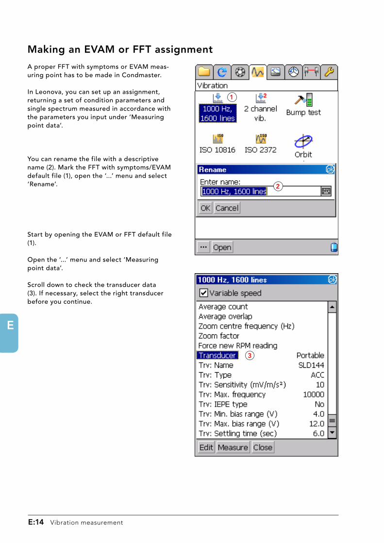
E
E:�� Vibration measurement
Making an EVAM or FFT assignment
A proper FFT with symptoms or EVAM meas-uring point has to be made in Condmaster.
In Leonova, you can set up an assignment, returning a set of condition parameters and single spectrum measured in accordance with the parameters you input under ‘Measuring point data’.
You can rename the file with a descriptive name (2). Mark the FFT with symptoms/EVAM default file (1), open the ‘...’ menu and select ‘Rename’.
Start by opening the EVAM or FFT default file (1).
Open the ‘...’ menu and select ‘Measuring point data’.
Scroll down to check the transducer data (3). If necessary, select the right transducer before you continue.
�
�
�

E
Vibration measurement E:��
To evaluate a spectrum, you need to know the RPM of the shaft at the time of vibration measurement. Mark ‘Variable speed´ (1). This forces a speed measurement before you can measure the vibration.
With ‘Measuring point data’ you can edit the measuring parameters. Mark the lines in the configuration window one by one. Open them with the EDIT button (2). The transducer setting ‘Portable’ selects the default trans-ducer. ‘Signal unit’ is the unit for the time signal, while ‘Spectrum unit’ is the measuring unit for the spectrum (e. g. VEL for a velocity spectrum).
Frequency rangeThe frequency range (3) is defined by selecting a lower and an upper limit. Both are menu selected.
Please note that correct measurement demands a transducer that is linear over the stated frequency range.
Abnormally high displacement values can occur when selecting a lower frequency limit that is outside of the transducer’s range.
You can exceed the upper frequency range of the transducer when measuring an envelope spectrum.
Signal unitAs signal unit (unit for the time signal) you can select VEL, ACC or DISP (4).
Spectrum unit As spectrum unit (5) you can select VEL, ACC or DISP. Normally you would choose a velocity spectrum, i. e. VEL.
Defining the assignment
�
�
�
�
�
�
�

E
E:�6 Vibration measurement
�
��
��
�
WindowTo compensate for the leakage effect intro-duced by the FFT process, a window function is usually applied. The user should choose the appropriate window (1) function for the specific application. If the windowing is not applied correctly, errors may be introduced in the FFT effecting amplitude, frequency or even the overall shape of the spectrum.
- Flat-top. The Flat-top window should be applied on sinusoidal signals. This window has the best amplitude accuracy, but poor frequency resolution.
- Hanning/Hamming. The Hanning and
Hamming windows are best for random signals. These windows have good frequency resolution and also rather fair amplitude accuracy. Since the Hanning window also has somewhat lower spectral leakage, this window is usually the one to prefer.
- Rectangle. The Rectangle (None, Uniform) window is the one to choose for transient signals. The Rectangle window has the best frequency resolution but poor amplitude accuracy and high spectral leakage.
As general advice, use:
- Hanning window for frequency accuracy (this is the most common window to use).
- Flat-top window for amplitude accuracy.
- Rectangle window only on transient signals.

E
Vibration measurement E:�7
FFT typeFour different FFT types (2) can be selected:
‘Linear spektrum’ consists of RMS values on a linear scale. Each value is the equivalent of the RMS value of a sinusoidal signal of the correspondent frequency. If the spectrum unit is velocity, v, the amplitude scale is accordingly: vrms.
‘Power spectrum’ (Autopower). Each value is the equivalent of the RMS square value of a sinusoidal signal of the correspondent frequency. If the spectrum unit is velocity, v, the amplitude scale is accordingly: v2
rms.
‘Power Spectral Density’ (PSD). This is a power spectrum where each amplitude value is divided by the FFT line width times the used windows equivalent noise band width. If the spectrum unit is velocity, v, the amplitude scale is accordingly: v2
rms/Hz.
‘Amplitude spektrum’ is closely related to the Linear spectrum scale. The Amplitude spectrum shows the peak value instead of the rms value. If the spectrum unit is velocity, v, the amplitude scale is accordingly: vpeak.
As general advice, use:- Linear or Power spectrum on periodic signals.- PSD spectrum on non-periodic (noise) signals.
Number of spectrum lines The number of spectrum lines (3) affects the resolution and the measuring time. Doubling the number of lines also doubles the measuring time. In cases where different fault symptoms, such as bearing frequencies and multiples of 1X, are close together, a high resolution spectrum is preferred.
Spectrum to saveSaving a time record or a full spectrum requires more memory. Unless the spectrum lines in damage patterns have fairly high amplitudes, the pattern is not visible.
Thus, saving only peaks will preserve the essential data while reducing the amount of redundant data. A peak is a spectrum line that has a line with a lower amplitude on either side.
If you select ‘Peaks’ under ‘Save’ (4), Leonova will display the full spectrum before saving, with the peaks as black lines while the lines to be deleted are grey. The maximum number of peaks that can be saved is half the number of spectrum lines. The number of peaks to be saved (5) is input on the number pad.
For the 2 channel analysis, you do not work with zoom and envelo-ping.
�
�
�

E
E:�8 Vibration measurement
Enveloping filterEnveloping is a technique used to detect low energy vibration typically caused by gear and bearing damage. This type of damage tends to modulate the amplitude of high frequency vibration, e. g. at the natural frequency of the transducer.
To suppress all vibration in the lower frequency ranges, a high pass filter is set at 1000 or 2000 Hz (1).
Average typeTo achieve greater accuracy, one can order the average result (2) from a stated number measure-ments (average count, set on the number pad). To get a time synchronous average, a tachometer must be connected which supplies a trigger pulse. This starts each measurement with the shaft in the same position. ‘FFT linear’ gives the mean value of the measurements, while FFT peak hold gives the maximum value.
Average overlapTo achieve faster collection of measuring values, one can activate ‘Avearge overlap’ (3). This func-tion will reduce the measuring time by using less time waveform data to produce the spectrum.
Zoom centre and zoom factorTrue zoom (4) is selected to get a high resolu-tion around a selected ‘centre frequency’. This frequency must be within the selected frequency range. Thus, to zoom in on 600 Hz, the minimum range is 0 to 1000 Hz. The range covered by the zoom is ‘upper frequency range/zoom factor’. Thus, with a zoom factor of 10, the spectrum will cover the range 550 - 650 Hz.
The highest possible zoom corresponds to a 12800 line spectrum. For this, combine the lowest number of spectrum lines, 400, with a zoom factor of 32 (32 x 400 = 12800). With a centre frequency of 600 Hz, you will get a spectrum over the range 584.375 to 615.625 Hz, with a resolu-tion of 0.078125 Hz.
�
�
�
�
�
�
�
�

E
Vibration measurement E:��
Measurement results
After measuring vibration, Leonova will display the three main condition parameters DISP, VEL and ACC.
The status dots (1) are grey because there are no evaluation criteria for EVAM assignments set up in Leonova.
The full list of condition parameters (2) is shown in the measuring result window.
Peak and peak to peak values are displayed for the signal unit (i. e. ACC when an accelerometer is used).
The spectrum is displayed in the selected spectrum unit, here velocity.
Tapping with the stylus on ‘Hz’ (3) toggles between Hz, CPM and, if rpm is measured, orders.
For spectrum functions in Leonova, see part B of this manual.
�
�
�

E
E:�0 Vibration measurement
� channel simultaneous vibration monitoring
Two channel simultaneous vibration monitoring requires that either the measuring technique ’FFT with symptoms’ or ’EVAM’ is active.
This type of measurement allows you to study machine movement in two dimensions by observing the difference of the phase angles measured on the two channels.
Measurement requires the set-up of two vibration assignments with identical parameters. Select transducers to be used in the transducer register under ‘Settings’, see page A16. The 2 channel measuring cable CAB51 is used to connect both transducers to the Leonova vibration transducer input.
You make an EVAM or FFT assignment, then select the Two channel mode and attach the same assign-ment to both transducers.
The procedure is the same as for the corresponding measurement with a single transducer.
To change frequency and spectrum lines, mark the line ‘2 channel vib’ (1) and select ‘Measuring point data’ under the button ‘. . .’ (2). Select channel and press the edit button.
To evaluate a spectrum, you need to know the RPM of the shaft at the time of vibration measurement. Mark ‘Variable speed´ (3). This forces a speed measurement before you can measure the vibra-tion.
To edit the measuring parameters, mark one of the channels (4) and select ‘Measuring point data’ under the ‘. . .’ button. Mark the lines in the configuration window one by one and open them with the EDIT button. See under ‘Defining the assignment’ earlier in this chapter
Most of the parameters must be the same for both channels. Changing will affect both channels.
For the 2 channel analysis, you do not work with zoom and enveloping.
2 channel measuring cable CAB51
�
�
�

E
Vibration measurement E:��
�
After measurement, Leonova displays the RMS values for DISP, VEL and ACC for both channels. Mark one of these results to get the corresponding measuring result diagram or spectrum.
In the spectrum window, three graphs are available under ‘...’ (1):
• Spectrum• Phase spectrum• Time signal
A phase is a time delay expressed in degrees of rotation. Leonova calculates the time delay between the passage of the tachometer pulse and the peak of the frequency component of interest from the vibration transducer at the speed of rotation. The value presented is a relative angle, not an absolute, because there is no compensation for phase lag in the transducer or the electronic circuits.
In the spectrum and the time signal, the channels are overlayed red and blue.
Tap and hold to produce the blue marker (2) in the spectra. For the marker position, the frequency, the amplitudes for both channels and the phase angle are displayed (3). Move the marker with the right/left arrow keys.
A marker in the time signal will show the time and amplitudes for both channels. A period is selected by placing a second marker (4). Hold down SHIFT, then tap and hold in the second marker position. With an overlay of both channels, the delta time and frequency for the period are displayed, plus delta amplitudes for both channels and the delta phase angle between them (5).
More about spectrum and time signal functions are described in chapter B.
�
�
� channel simultaneous vibration results
�
�
�

E
E:�� Vibration measurement
Run up /coast down
To make either a ‘Run up’ (from machine start to working speed) or a ‘Cost down’ (from working speed to stop) measurement, select the vibration menu and then the function ‘Run up/Cost down.
Measuring points can be downloaded from Cond-master. The parameters are set in the instrument, then uploaded to Condmaster where the measure-ment results are saved as comments.
Select ‘Open’ to edit an existing measurement or ‘New’ to make a new measurement. For a new measurement, follow the guide (1).
Select the correct transducer (2). Edit transducer data if necessary. Mark the line to be configurated and open with ‘Edit’. When ready, press the arrow (1) to continue.
‘Signal unit’ (3) is what the transducer measures (ACC for accelerometers).
‘Spectrum unit’ (4) is the measuring unit for the spectrum (e. g. VEL for a velocity spectrum). Press the arrow button (1) to continue.
‘Lower frequency’ can be set from 0.5 to 100 Hz. The upper frequency i set in ‘Orders’, default 10 and can be changed via the number pad.
Select ‘Number of spectrum lines’ and ‘FFT window’. The choice of ‘Window’ (5) somewhat affects the spectrum line amplitudes. ‘Hanning’ (default setting) and Hamming are the window types most commonly used to calculate spectra. The difference is often marginal and should not affect pattern recognition.
‘Measurement interval’ can be RPM or time based (6). For time based it is essential to set a short time interval to get fast measurements enough to capture resonances that occurs.
For an RPM based measuring interval, set interval in RPM, for time based, in seconds (7) via the number pad.
‘RPM range’ for ‘Run up’ is low to high, for ‘Cost down’ it is high to low. Select the range via the number pad and continue to the measurement window with the arrow button (1).
�
�
�
�
�
6
�
7

E
Vibration measurement E:��
�
�
Connect the vibration transducer and the tachometer to Leonova. Press MEASURE. When measurement is completed, the measurement list (1) shows number of reading, time, RPM and RMS value. Press the arrow button to display the spectrum.
In the spectrum window (2) you can see each spectrum by marking the reading in the measurement list.
To display a waterfall diagram, press the ‘. . .’ button (5) in the spectrum window and select ‘Settings’. Select number of results to be shown in the diagram (6).
You can also select logarithmic scales and saved measuring result to be shown (7).
The waterfall diagram shows the marked reading in front. Tap and hold to produce the blue marker. For the marker position, orders, amplitude and phase angle are displayed (8).
More about spectrum functions are described in chapter B.
Run up /coast down measurement
�
�
7
6
8

E
E:�� Vibration measurement
The Nyqvist diagram (1) shows phase angle and amplitude for all readings as dots around the centre. Marked reading in the list is shown in the graph with a blue dot (2).
A phase is a time delay expressed in degrees of rotation. Leonova calculates the time delay between the passage of the tachometer pulse and the peak of the frequency component of interest from the vibration transducer at the speed of rotation. The value presented is a relative angle, not an absolute, because there is no compensation for phase lag in the transducer or the electronic circuits. The RPM is displayed in the list of measurements only.
‘Orders’ can be changed via the number pad (3)
The Bode diagram (4) shows ttwo separate diagrams with vibration amplitude (DISP, VEL or ACC) and phase angle on the Y axis, respectively, and RPM on the X axis. All measurements are displayed in time sequence. Marked reading in the list is shown in the graphs with blue dots.
The measurement can be saved under a file name.
�
�
�
�

E
Vibration measurement E:��
Bump test
The bump test is employed to check out the typical vibration response of a machine structure at stand-still, by hitting it e. g. with rubber mallet. To make a bump test on a stationary machine, select the vibra-tion menu and then the function ‘Bump test’.
A measuring assignment can be set up in Cond-master Nova for downloading to Leonova.
Select ‘Open’ to edit an existing measurement or ‘New’ to make a new measurement. For a new measurement, follow the guide (1).
Select the correct transducer (2). Edit transducer data if necessary. Mark the line to be configurated and open with ‘Edit’. When ready, press the arrow (1) to continue.
Select ‘Frequency range’, 100 to 40 000 Hz, and number of lines in the spectrum, 400 to 12 800.
‘Pre-trig’ sets the time before the trigger level is reached, in percent of the measuring time. It can be set to 5, 10, 15, 20 or 25%. Numbers within brackets is the corresponding time in seconds. The vibration during pre-trig time is included in the sample.
The sampling time is automatically calculated from the frequency range and the number of spectrum lines. Press the arrow button (1) to continue.
�
�
�
�
�
�

E
E:�6 Vibration measurement
During a bump test, Leonova measures continu-ously. A reading is saved when you hit the machine with e.g. a rubber mallet and the resulting vibration is within the set parameters.
The referential measurement is used to find the right trig level. The ‘Trig level’ (1) is set by hitting the machine frame with varying force. The peak amplitude of the measured signal is displayed (velocity in mm/s) and a trigger level can be set to 1% – 90% of the amplitude.
The green staple (1) shows the peak vibration level (blue arrow). The green arrow shows the trigger level.
Adjust the force of the hits if needed, or press CLEAR and repeat. When ready, press ‘Continue’ to go to the measurement window.
Press ‘Arm trigger’ to activate the measuring func-tion.
Hit with the same force as during the referential measurement. The actual test returns an FFT spectrum and a time signal (sampling time plus pre-trigging time).
Tap and hold to produce the blue marker (4). Move the marker with LEFT/RIGHT. At each step, the frequency, amplitude and phase angle are displayed.A marker in the time signal diagram shows the time and amplitude.
Under the ‘. . .’ button (5) you can select logarithmic scales for the X and Y axis.
The bump test can be saved under a file name by selecting ‘Save as’ when closing the vibration measurement window.
�
�
�
�
6
Bump test measurement
�

E
Vibration measurement E:�7
Orbit analysis
C
Orbit analysis is a vibration measurement function resulting in a two-dimensional orbit graph used to analyse shaft centerline movement, which may indicate rubs, unbalance, misalignment or oil whip, in machines equipped with journal bearings.
The data required for orbit analysis is a two channel simultaneous vibration measurement, where two displacement transducers are placed 90° from each other, and a trigger signal from a tachometer probe.
Measurements are normally made on the buffered outputs of a machine protection system via the Orbit Interface 15315. The interface is connected to the vibration and the tachometer inputs on Leonova. The signal inputs, channel X, channel Y and tachometer are connected via cables (SPM 15326) with BNC connectors.
Measurement with displacement transducers requires that two transducers are setup particular to the orbit analysis in the transducer register under ‘Settings’, see page A16.
Measurements can also be made with e. g. accelerometers, placed at an angle of 90° to each other, to get a two dimensional graph of machine movement. For measurement with accelerometer or velocity transducers, use the 2 channel meas-uring cable CAB51 or the Balancing Module 14745.
A measuring assignment for orbit analysis can be set up in Condmaster Nova and be downloaded to Leonova.
Select and open an Orbit assignment under the vibration flap. Set the Measuring point data under ‘. . .’ (1).
By pressing the button (2) it is possible to see the displacement of the X and Y values (3) when the machine is not rotating. This function is used to measure the displacement when adjusting the proximity probes.
Tachometer cable CAB10
Orbit Interface SPM 15315
3xBNC cables
SPM 15326
�
�
to VIB input
to TAC input
Machine protection system
�

E
E:�8 Vibration measurement
�
Variable speedMark ‘Variable speed’ (1) to force a speed measurement before measuring. For best results, it is strongly recom-mended that a measured rpm value is used in connection with orbit measurement.
Transducer typeCheck the data for the X and Y transducers. Press the button (2) and select the right transducers from the list (3). To change transducer data, mark a line and press the edit button (4).
For an 8 mm diameter proximity probe, the sensitivity is normally 7,87 V/mm (7,87 mV/µm). For other probes, please turn to the data sheet for information about their sensitivity.
Transducer data can not be changed when using portable transducers (5).
Open the window for configuration of signal unit, filter type and orders by pressing the arrow button (6).
Signal unitAs signal unit (unit for the time signal) you can select VEL, ACC or DISP (7). When measuring on buffered outputs of a machine protection system, ‘Signal unit’ must have the same setting as ‘Transducer type’.
Filter typeFor Filter type (8), the default setting is Bandpass, showing frequencies at rpm ±10%. With the filter type set to Lowpass, all frequencies above the selected multiple of shaft speed (Orders, 1-5) are filtered out.
Orders Orders is set to 1 by default, but can as high as 5 orders (9). The setting is used to calculate the center frequency for bandpass mode and the upper frequency for lowpass mode, respectively.
Number of revolutionsNumbers of revolutions, max. 25, specifies the number of shaft revolutions to acquire and display in the orbit graph (10).
RPM measurementMark RPM measurement when using a tachometer (11). If not, the rpm can be input via the number pad.
Settings for orbit analysis
�
�
�
�
6
�
7
8
�
�0
��

E
Vibration measurement E:��
During measurement, the orbit graph shows displacement in the X and Y direction per revolu-tion. When the measurement is complete, the average of the measured values is shown (1).
The orbit graph shows an overlay of the graphs for each measured revolution plus their average. Press the graph button (2) to get a close up of the graph.
When the orbit assignment is set up in Cond-master Nova, alarm limits can be set on the X and Y axis, resulting in an evaluated measure-ment (green - yellow- red scale) (3).
You can select each individual revolution as well as the average of all revolutions. Select the graph, marked dark blue, in the window (4).
With the button (5) you can activate an arrow (6) showing the angle and the peak value at that angle. You can move the arrow with tap and drag the stylus. The peak value and the angle are displayed (7).
Orbit measuring and results
�
�
�
6
7
�
�

E
E:�0 Vibration measurement

F
Rotor balancing F:�
Rotor balancing
Contents
Balancing methods ................................................................ 3
Balancing equipment ............................................................. 4
General settings .................................................................... 6
Selection of vibration transducer .......................................... 7
Unbalance .............................................................................. 8
Measuring unbalance ............................................................. 9
Four run method .................................................................. 10
Two run methods ..................................................................11
Transducer selection and spectrum measurement .............. 12
Run without trial weight ...................................................... 13
Trial weight calculation ........................................................ 14
Run(s) with trial weight ........................................................ 15
Display of results ................................................................. 16
Alternatives for balancing weights ...................................... 17
Trial run and log ................................................................... 18

F
F:� Rotor balancing

F
Rotor balancing F:�
Balancing methods
Single and dual plane balancing are optional Leonova functions with either limited or unlimited use. In case of limited use, credits are deducted for each vibra-tion measurement.
Single plane balancing, 4 runs
This method uses one measurement without trial weight to determine the vibration severity (mm/s RMS) of the rotor, followed by three measurements with trial weights at 0°, 120° and 240° to calculate the weight and position of the correction mass. No rpm measurement is needed but all measurements must be done at the same rpm.
Single plane balancing, � runs
This method uses one measurement without trial weight to determine the vibration severity (mm/s RMS) of the rotor, followed by one measurements with a trial weight to calculate the weight and position of the correction mass. It requires time synchronised vibration measurement (trigger pulse supplied by a pulse from the SPM tachometer probe or a proximity switch) to find the relative phase angle between the two vibration measurements.
Dual plane balancing
The same 2-run method as used for single plane balancing, but with vibration measurement and weight correction in two planes. These measurements can be made by shifting the vibration trans-ducer or by connecting two transducers via the 2 channel measuring cable CAB51. Please note: To get a good result fast, the static unbalance must be corrected before starting the dual plane balancing with Leonova.
For all methods, a final run can be made to check the balancing results and, if needed, get the data for further adjustments. Leonova then saves a balancing log file.
Leonova guides step-by-step through the balancing procedure. One can shift the rotation direc-tion and change the measured parameter from velocity to acceleration or displacement.
In addition to the RMS value, a spectrum is shown to help find the part of vibration that is due to unbalance. For the 2-run methods, the number of samples for obtaining a time synchronous aver-age is set to min. 4.

F
F:4 Rotor balancing
Balancing equipment
For single plane balancing with four runs, the only equipment needed is a vibration transducer type SLD144 or an IEPE (ICP®) type transducers with voltage output.
The transducer is mounted with a magnetic foot (TRX16) or with an M8 (UNC 1/4”) screw. It is connected with the spiral cable CAB48 or a straight cable CAB48-L (L = cable length in meters).
For the 2-run methods, a trigger pulse is needed which is either given by a proximity switch or by the SPM tachometer probe TAD18. When using a proximity switch, the Balancing Module 14745 can be used. This module also allows connection of two vibration transducers.
The light beam from the tachometer probe is directed towards a piece of reflecting tape pasted on the shaft. The tape must have a sharp edge.
It is very important that the tachometer probe is firmly at-tached and not moved during the balancing procedure.
SPM supplies a tachometer probe holder with a magnetic base (SPM 81319) and a clamp for the probe (SPM 14765), plus a 5 m long tachometer probe cable (SPM CAB43).
The 2 channel measuring cable CAB51 allows the connection of two vibration transducers to Leonova. These must be of the same basic type, e.g. IEPE with voltage output. Dual plane rotor balancing can be done with a single transducer, but using two is faster.
Transducer SLD144with magnetic foot
81319
14765
CAB48
TAD18
CAB43 CAB51
CAB48-L

F
Rotor balancing F:�
General settings
To start with, go to the TOOL menu and open GENERAL SETTINGS, then the BALANCING menu.
Your selection under ‘Counter rotational degrees’ affects the way the angles are displayed while balancing.
When the box is not marked, angles are displayed as shown in figure A.
When the box is marked, angles are displayed as shown in figure B.
Marking ‘Ounce’ will show all weights in ounces instead of grams.
‘Output unit’ is the transducer output, ACC VEL or DISP.
Rotational0°
Counter rotational0°
+ 90°
+ 90°
A
B

F
F:� Rotor balancing
Selection of vibration transducer
The ‘Registration of vibration transducers’ is described in Part A of this manual. Before starting vibration measurements, make sure that the vibration transducer you are using with your Leonova is properly registered, configured and selected.
The nominal sensitivity of a vibration transducer SLD144 is 10 mV/m/s2. The actual sensitivity of the individual transducer is written on its calibra-tion card. This data should always be input in the transducer register (1). When several transducers are in use, they should be marked to assure that the readings are calibrated.
To select a transducer, open ‘Vibration transduc-ers’ in the TOOLS window. Mark its name on the list (2) and touch the arrow key (3). To see or edit its data, mark its name on the list (2) and touch the edit button (4).
To change data, mark the line and click the ‘Edit’ button (5).
For ‘Dual plane’ balancing, two transducers are selected from the ‘Transducer register’ as default. Press the button (6) and select two transducers to be used (7). The transducers must have the same output (DISP, VEL or ACC).
�
�
�4
�
�
7

F
Rotor balancing F:7
Unbalance
A rotor is unbalanced when the centre of its mass does not co-incide with the shaft centre.
This condition can be described as the rotor having a ‘heavy spot’ somewhere along its circumference.
If we know the position and weight of this heavy spot, we can reduce it by taking away mass or, more often, put a counter-weight on the oppisite side of the rotor.
For one plane balancing, it is assumed that the heavy spot is on the centre line of a narrow rotor or near enough, so that it does not matter on which side of the centre line the counter weight is place.
For rotors which are wide in relation to their diameters, we assume two heavy spots in the rotational planes at both ends of the rotor.
The counter weights and their positions are calculated with regard to the interac-tion between both planes.
Position?
Counter weight?

F
F:� Rotor balancing
Measuring unbalance
Unbalance causes excessive vibration. However, excessive vibration can have any number of other causes. Thus, before attempting to balance a rotor, we must first check that there is an unbal-ance problem and make sure that other vibration causes, such as loose parts and misalignment, are eliminated.
As the ‘heavy spot’ rotates in the radial plane, the vibration values measured in horizontzl (H) and vertical (V) should be higher than the vibration measured in the axial direction (A).
Check all three directions. For balancing, measure in direction H or V, whichever yields the highest value.
Unbalance causes vibration with a frequency of 1X, which is the shaft frequency in Hz (rpm/60), also called the first order.
Check that the vibration spectrum has a clearly dominant line at 1X . This line is marked in the Leonova balancing spectrum.
All three balancing methods use a first run to establish the vibration behaviour of the rotor.
The following run is made with a trial weight fas-tened at a convenient spot along the rotor. Thus, we add a known unbalance factor, which allows us to calculate the position and weight of the unknown ‘heavy spot’ from the change in vibration behavour.
1X
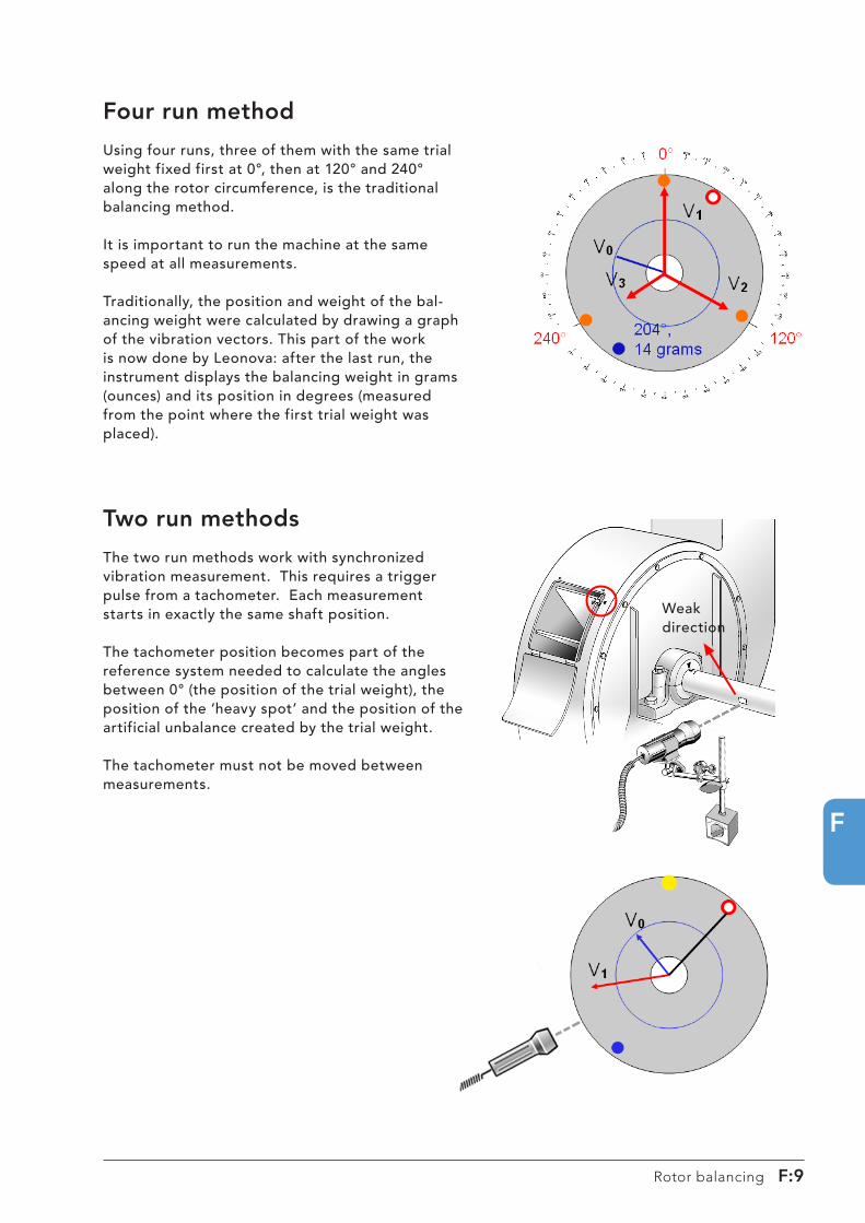
F
Rotor balancing F:�
Four run method
Using four runs, three of them with the same trial weight fixed first at 0°, then at 120° and 240° along the rotor circumference, is the traditional balancing method.
It is important to run the machine at the same speed at all measurements.
Traditionally, the position and weight of the bal-ancing weight were calculated by drawing a graph of the vibration vectors. This part of the work is now done by Leonova: after the last run, the instrument displays the balancing weight in grams (ounces) and its position in degrees (measured from the point where the first trial weight was placed).
Two run methods
The two run methods work with synchronized vibration measurement. This requires a trigger pulse from a tachometer. Each measurement starts in exactly the same shaft position.
The tachometer position becomes part of the reference system needed to calculate the angles between 0° (the position of the trial weight), the position of the ‘heavy spot’ and the position of the artificial unbalance created by the trial weight.
The tachometer must not be moved between measurements.
Weakdirection

F
F:�0 Rotor balancing
Transducer selection and speed measurement
The balancing procedure is menu guided. Select the method, then simply follow the instructions on the screen.
The first steps are common for all methods. Start with selection of transducer(s). The transducer(s) selected under ‘Transducer register’ will come up as default.
For the ‘Dual plane’ method, two transducers can be used. Mark the box ‘Balancing module’ (1). The two transducers must have the same output (DISP, VEL or ACC).
Follow the setup guide by pressing the arrow key (2) and then measure without trial weight to obtain the vibration severity and the spectrum.
For the ‘4-run’ method, the RPM data are only needed to find the 1X position in the spectrum and thus check on the amount of unbalance. You can do without the RPM, input it via the numbers pad, or measure it (asynchronous measurement).
The ‘2-run’ methods are automatically set for synchronous RPM measurements, see previous page. You can input the number of synchronized readings.
�
�

F
Rotor balancing F:��
Set the frequency range for the spectrum to ‘au-tomatic’. Leonova will calculate the suitable range from the RPM data.
With the tachometer and the vibration transducer connected, click on ‘Measure’.
Click on the spectrum symbol (1) to display the spectrum. To set a marker (2) on the spectrum line at 1X (which shows the amount of unbalance), click the button (3), select ‘Settings’ from the menu and activate ‘Theoretical symptom’.
In case the 1X line is relatively small, abort balanc-ing and first check the machine for other vibration causes (misalignment, loose bolts, etc.).
For all methods, the run without trial weight supplies the value for V0 (4), the initial machine vibration.
4
Run without trial weight
�
�
�

F
F:�� Rotor balancing
The trial weight has to be large enough to create an unbalance but must not be so heavy as to create dangerous vibrations.
Open the calculator (1) and use Leonova to calculate a suitable weight. The input data are the approximate weight of the rotor and its diameter.
Input the mass of the trial weight with the number pad (2).
For dual plane balancing, you use two trial weights, one for each plane. They can have different masses.
Trial weight calculation
��

F
Rotor balancing F:��
Run(s) with trial weight
The position where the trial weight is attached automatically becomes the 0° position on the rotor. All angles are given with this point as a reference.
For the 4-run method, you first measure V1 with the trial weight at 0°, then V2 with the weight at 120° and finally V3 with the weight at 240°.
For dual plane balancing, first measure V0 (with-out trial weight) in plane 1, then in plane 2.
You then fasten the trial weight in plane 1 and measure V1 in plane 1, then in plane 2.
You normally remove the trial weight from plane 1 before attaching the other trial weight in plane 2. If not, mark the box ‘Keep trial weight’ on the menu. Measure V1 in plane 1, then in plane 2.
4-run method, menu during third run
2-run method, menu during run with weight

F
F:�4 Rotor balancing
The calculation results are the mass of the balancing weight and the angle defining the position where it has to be attached.
The display shows the direction of rotation and the position of 90°.
On the side of the display (1) there is a row of function keys that allow you to select alternatives to adding mass at the indicated spot.
Display of results
Calculation results, 4-run method
Calculation results, dual plane
�

F
Rotor balancing F:��
Graphical check of calculation results.
Split the correction mass: Input the number of rotor partitions to distribute the correction mass between two of them.
Radial displacement: Input the change in radial distance to recalculate the weight.
Calculate radial position of smaller/larger balancing weight.
Weight removal: Show drill hole position.
Degrees to length: change from angle to length measured along the rotor circumference.
Sum up weights: Replace all correction masses on the rotor by one.
Weight removal: Drill hole diameter and depth calculated for various materials.
Alternatives for balancing weights
Leonova calculates a number of alternatives for correcting the unbalance:

F
F:�� Rotor balancing
Trial run and log
After balancing weight application, a trial run can be made to measure vibration after balancing. If balancing was successful, the vibration at 1X should be considerably lower.
The information in this window is optional. It will appear in the balancing log file.
In case you used the proposed weight and posi-tion, press ‘Copy to log’ to input the data.
To print out an balancing report, do the following:
• Connect Leonova to the PC.
• Start the Leonova Service Program and select ‘Print balancing report’ (1).
• Select balancing file saved under the ‘FILE’ menu.
• Select printer, number of copies, etc under the ‘Print out’ menu.
�

Shaft alignment G:�
G
Shaft alignment
ContentsShaft alignment with Leonova ............................................... 3
Shaft alignment equipment ................................................... 4
LineLazer detectors ............................................................... 5
Alignment kit attachment ...................................................... 6
The detector panel ................................................................ 6
Charging batteries ................................................................. 7
Communication with Leonova ................................................ 7
Shaft alignment .................................................................... 8
About shaft alignment .......................................................... 9
Means for horizontal movements .......................................... 9
Alignment – general procedure ........................................... 10
Settings ................................................................................11
Compensation ..................................................................... 12
Alignment tolerances ........................................................... 12
Basic data input ................................................................... 13
Input distances .................................................................... 13
Soft foot .............................................................................. 14
Measuring (automatic or manual input) ............................... 15
Result window...................................................................... 16
Feet lock .............................................................................. 16
Alignment work using the Alignment window ..................... 17
Alignment – vertical machines ............................................. 18
Settings ............................................................................... 18
Basic data input ................................................................... 19
Measuring ............................................................................ 19
Measuring results ................................................................ 20
Alignment work using the Alignment window ..................... 21
Create report ....................................................................... 22

G
G:� Shaft alignment

Shaft alignment G:�
G
Shaft alignment with Leonova
Shaft alignment is an optional Leonova function, supported by Leonova MMI software version 3.00 or higher, with either limited or unlimited use.
Under the assignment flap (1) Leonova contains two standard alignment assignments, one for horizontal (2) and one for vertical (3) machines, with functions for soft foot, feet look and com-pensation for thermal growth.
An alignment can be saved as a file (4) with all basic data, to be used again for similar machines.
The Leonova Alignment kit consist of LineLazer detector/transmitter units that measures the position of the shafts compared to the centre line. They have position detectors (PSDs) with large vertical reception area, receiving a horizon-tal line laser beam, with makes fine tuning almost unnecessary. Integrated precision inclinometers measure the angle of rotation of both detectors at all times. This allows measurement in fully automatic mode, with much less than a half-turn of the shaft. Measurement results are displayed in 100ths of a millimetres or 1000ths of an inch. Only the master detector is connected to Leonova. One cable is eliminated due to wireless communication between the master and the slave detector.
Leonova is the control and display unit. The interaction between the graphical display and user is kept as simple as possible. A self-explana-tory display based on icons and graphics guides the user, step by step to a correct alignment. A live view shows immediately the result of the vertically and horizontally corrections. A pre-programmed tolerance table tells the user when proper alignment is achieved. A green – yellow – red dot shows the severity of the misalignment, or when the result is within the tolerances. Le-onova produces a log file with all alignment data for printing a report.
�
4
��

G
G:4 Shaft alignment
Shaft alignment equipment
LLB10
LLB14
LLB13
LLB15
LLB12
LLB11
CAB50
CAB45
MAA70
TOL21
LineLazer Accessory Set LLA��0
The LineLazer Accessory Set contains detector/transmitter units, brackets, chains, rods, cables and a measuring tape, all in a carrying case. This set fits a multitude of applications, e.g. compressors, gear-boxes, generators, and pumps.
LLB10 LineLazer detector/transmitter unit
LLB11 Extension chain, length 1000 mm
LLB12 Chain with tension adapter, length 500 mm
LLB13 Supporting rod, 80 mm, set of 4
LLB14 Supporting rod, 150 mm, set of 4
LLB15 Shaft bracket for chain
CAB50 Communication cable between LineLazer and Leonova, length 3 m
CAB45 Charger cable, length 1.5 m
MAA70 Measuring tape
TOL21 Torquing tool for chains and rods
CAS18 Carrying case, plastic with foam insert
Battery charger
90340 Charger, 100-240 V AC, 50-60 Hz, EU-plug
90348 Charger, 100-240 V AC, 50-60 Hz, US-plug
90349 Charger, 100-240 V AC, 50-60 Hz, UK-plug
Options
Magnetic brackets, offset brackets 50 mm and offset brackets 100 mm on request.
Spare parts
LLB20 Supporting rod, 80 mm
LLB21 Supporting rod, 150 mm

Shaft alignment G:�
G
LineLazer detectors
Laser transmitter
Position detector (PSD)
NB: Never stare directly into the laser transmitter.
Using a horizontally spread laser beam in com-bination with a 37 mm vertical detector (PSD) makes fine tuning unnecessary. The laser beam is modulated and thus easily and automatically distinguished from interfering light sources. The laser beam is not mirrored, both units are true detectors/transmitters. The communication between them is wireless, only one of the units, designated as ‘master’, is cable connected to Leonova.
The detector units have integrated double axis precision inclinometers which measure the angle of rotation of both detector units at all times. This means that the shaft can be rotated at will in both directions. A measurement can be taken automatically when the shaft movement stops (automatic mode) or ordered by a ‘Measure’ command (manual mode). Measurement results are displayed in 100ths of millimetres or 1000ths of an inch, angles in steps of 0.1°.
Please note: Other position measuring devices can be used. In such cases, ‘user input mode’ is selected and both angles and clock readings are input via keypad.
Laser type: line laser, visible red light
Laser power : <1 mW
Laser safety class: Class 2
Laser wavelength: 635 to 650 nm
Laser modulation: 200 kHz
Sensor resolution : 1 µm
Sensor linearity : < 2% deviation
Sensor size : 37 x 1 mm
Operating range : 50 to 3000 mm (2 to 120 inches)
Inclinometer resolution : 0.1°
Battery: NiMH rechargeable
Operating Time : > 8 hours normal use
Operating Temperature: 0 to 50 °C
Storage Temperature: -10 to 60 °C, non condensing
Keyboard: sealed membrane
Control indicators: LED
Connector type: LEMO for communi-cation with Leonova and charger
Housing: aluminium, black anodized
Protection: IP65
Dimensions: 112 x 93 x 44 mm
Weight: 550 g
Technical specifications for LineLazer

G
G:� Shaft alignment
LED
ON / OFFbutton
Input for communica-tion and charger cable
LED indicators
Alignment kit attachment
TOL21ø 4 mm
Locking screws
As default, the motor is defined as M (movable, 1) and the other part, here the pump, as S (stationary, 2) machine. The view depicted on the Leonova screen is from the motor fan end (none-driven side, 3). The master detector unit (with the cable, 4) is placed on the M machine. Please note that all this can be changed at will, as long as the inputs under ‘Settings’ agree with the way the kit is mounted.
Attach the detector units as shown, firmly but without undue force. Use the enclosed tool when tightening the rods.
These are the parameters:
• Max. shaft diameter with 500 mm chain = 165 mm (6.5 inches), with 1000 mm extension chain = 480 mm (18 inches).
• Distance between detector units = 50 to 3000 mm (2 to 120 inches).
• The minimum recommended angle of shaft rotation is 180°.
The detector panelThe detector panel has an input connector for com-munication with Leonova and for battery charging, and a switch for power ON/OFF.
A blinking green LED for communication and steady green LEDs for detector position and bat-tery OK show that the detectors are adjusted for measurement. For various other states, see the table below.
��
�
4
GREEN LIGHT RED LIGHTFixed Blinking Fast blinking Fixed BlinkingLaser on Communication Laser fault with Leonova Battery OK Battery low Battery empty Charging Charging trickle modeAngle of both System Temperaturedetectors OK failure out of range

Shaft alignment G:�
G
Charging batteries
CAB50
CAB45
LineLazer charger90340, 90348 or 90349
Communication with Leonova
The batteries are recharged with the chargers SPM 90340 (EU), 90348 (US) or 90349 (UK).
The battery LED is red when charging and starts blinking red when the batteries are fully charged (trickle mode).
Battery type: NiMH rechargable
Operating Time: > 8 hours normal use
Charging time: approx. 1.5 hours (may vary depending on the ambient temperature and the condition of the batteries).
Do not replace the batteries. Refer servicing to your local SPM dealer.
After connecting the communication cable between the master detector and Leonova, it should be clamped to the fixture, so that it cannot put any strain on the detector when the shaft is turned.
Please note that the detector units are identical; the master being the unit that is connected to Leonova. Do not switch the cable during align-ment.
When both detectors are ON and the master detector is connected to Leonova (also ON), the laser intensity LED starts blinking green for communication with Leonova. The OK LED is green on both detectors when they are aligned within the tolerances, ± 2°.

G
G:� Shaft alignment
Shaft alignment
Symptoms of misalignment
The purpose of shaft alignment is to prevent excessive vibration and the premature failure of machine parts.
Quite often, bad machine condition is obvious, but repairs are made without correcting alignment faults, or removing the underlying causes for misalignment, such as poor foundations, excessive temperature gradients, strain from connected pipes, etc.
An alignment check should be made if one or more of these symptoms are noted:
• excessive radial and axial vibration• high oil temperature, hot bearings• excessive oil leakage at the bearing seals• loose foundation bolts• loose or broken coupling bolts• hot coupling immediately after shutdown• with elastic couplings, rubber or plastic
powder inside the coupling guard• frequent bearing and/or coupling failures.
Explanation of terms
Shaft alignment – the process of adjusting the rela-tive position of two coupled machines (e. g. a motor and a pump) so that the center lines of their shaft form a straight line when the machine is running at normal operating temperature.
Alignment is achieved by moving the front and/or back feet of one machine up, down, and sideways, until the shafts are aligned within required tolerances. Normally, the other machine remains stationary. However, as one cannot lower a machine below its foundation, it may be necessary to shims the ‘station-ary’ machine to achieve alignment.
Soft foot - the condition when the machine is resting on three feet instead of all four. The soft foot has no proper contact with the machine foundation. Prior to alignment, soft foot is eliminated by placing shims under the foot until the machine is properly sup-ported.
Center linesaligned
Soft foot
Shims
Typical misalignment symptom

Shaft alignment G:�
G
About shaft alignment
Misalignment – the condition when the center lines of the shafts are not aligned within tolerances.
There are two types of misalignment:• Offset - the center lines of the two shafts are parallel
but do not meet in a common point at the center of the coupling.
• Angularity - the center lines meet at the center of the coupling but are not parallel.
Both offset and angularity can, and normally do, occur simultaneously.
Misalignment is measured in two planes, vertical (up, down), and horizontal (sideways). Thus, there is:• vertical offset• horizontal offset• vertical angularity• horizontal angularity.
Normally, shaft misalignment is a combination of all four of these alignment faults.
Note that the object is to align the shafts and not the coupling. If a coupling half is bored slightly off center, aligning the coupling will cause misalignment of the shafts.
Means for horizontal movements
Moving a heavy machine sideways for an exact distance is not easy, if one tries to do it with a sledge or a crow-bar.
Much time can be saved by preparing the footplate of the machine to be moved for horizontal adjustments of the machine position. The general idea is to move the machine by turning a screw, instead of lifting, hitting, or pushing it, see figure A.
Figure B shows a simple, portable ”moving aid” which is bolted to the foot plate. This device is only used for alignment work, so it is no obstacle during normal machine operation. Correctly made, it can be used for many different machines.
A
B
Offset
Angularity
Offset and angularity

G
G:�0 Shaft alignment
Alignment – general procedure
� �� 4
The need for alignment should be established by means of vibration measurement, see page 8. Prior to alignment, inspect and, if needed, repair the machine foundation.
• Mount the alignment kit on the shafts or the coupling (see page 7), define M = machine to be moved, normally the motor.
• Switch on Leonova and open the alignment file (mark and touch OPEN).
• Connect the detector unit on the machine to be moved (M) to Leonova. This is the master. Switch on the detectors (button on top) and align them in such a way that the centre of the laser beam is in the centre of the target area.
The detector LEDs should light up as shown.
• Open the ‘Settings menu’ (1) and set the general alignment parameters (page 11). Under ‘Compensation’, input the values for thermal expansion (page 12).
• Open the ‘Data window’ (2) and input the distances (see page 13).
• Measure and correct softfoot (page 14).
• Open the ‘Measurement window’ (3), meas-ure alignment (see page 15).
• Open the ‘Result window’ (4), check present position (see page 16).
• Open the ‘Alignment window’ (5), shims as required, then make horizontal adjustments (see page 17).
• Go to the ‘Measurement window’ (3), meas-ure alignment results.
�
LASERBlinking green
BATTERYFixed green
SYSTEMFixed green
Ready for measurement:

Shaft alignment G:��
G
Settings
The alignment program starts in the ‘Data window’. General parameters can be changed in the Settings window (open by touching the ‘...’ button, then ‘Settings’). To make changes, touch a line, then ‘Edit’. Finish with ‘Close’. Your settings will be preserved when you close the alignment function.
Method
Method determines the measuring mode. In ‘Automatic’ mode the measuring starts automatically when the detec-tors are in position. After that, you wait until the results are displayed. Then the shaft is turned and kept steady in the new position until the next reading is displayed. This operation, turn and hold, is repeated until the detectors have been moved through about 180° and at least 3 meas-urements have been taken. Please note that if the shaft is turned less than 5° the new measurement will replace the earlier.
‘Manual’ is similar except that the ‘Measure’ key on Leonova is pressed each time the shaft has been rotated into a new position.
‘User input’ is selected when the LineLazer detectors are not used. The clock angles and readings are input via the number pads.
General
No. of decimals: Default is 2 decimals for distances in mm, 3 decimals for inches. Angles are always displayed with one decimal.
Master indicator: Select S or M, depending on which detector is connected to Leonova.
Tolerance table: The default tolerances can be helpful if no limit values are available from the manufacturer.
Average screen update: The LineLazer detectors measure three times per second. The displayed result is an average of the number of measurements input under ‘Average Screen update’
Average measurement: The saved result is an average of the number of measurements input under ‘Average Measurement’ . The range is 2 - 15 for all methods.
Tolerance table: Select a suitable tolerance table. If no limit values are available, use the default tolerances in Leonova.
RPM: The input under RPM determines the selection of the alignment tolerances - the higher the RPM, the narrower the tolerances.
Coupling: Select coupled or uncoupled machine. Use uncoupled to see both inclinometer values.
Directional view determines how shaft rotation angles are displayed: ‘None driven end’ means as seen from the motor fan end.
Angle selection is either 0 to 360° or 0 to +180° (clockwise via 3.00 hours to 6.00 hours) plus 0 to -180° (counter clockwise via 9.00 hours to 6.00 hours).
View adjustment: ‘Graphics’ means that a motor/pump drawing is shown in the Result window, replaced by lines when ‘Lines’ is active.

G
G:�� Shaft alignment
Compensation
Different rates of thermal expansion in the M machine relative the S machine can have a considerable effect on horizontal shaft alignment. For an electric motor, the vertical thermal expansion is approximately 0.1 mm per meter for each 10° C rise in temperature. Example: Height foundation - shaft: 500 mm Alignment temperature: +20° C Operating temperature: +50°Thermal expansion: 0.5 x ((50 - 20)/10) x 0.1 = 0.5 x 3 x 0.1 = 0.�� mm
If the S machine has the same thermal properties as the M machine, there is no problem. If there is a significant difference, one can either try to align the machines before they cool, or one has to compensate for the difference. Thus, if the S machine is going to rise an extra 0.2 mm when hot, use a 0.2 mm compensation for the M machine.
Manufacturers will normally supply data on their machines’ thermal properties. When estimating thermal rise, check• operating temperature of both machines• thermal expansion of both machines• environment influences on machine temperature, such
as strong sunshine and other heat sources, effect of cooling systems, etc.
Alignment tolerances
Alignment tolerances depend largely on the rotational speed of the machine.
Machinery should be aligned within the tolerances stated by the manufacturer. If no limit values are avail-able, use the default tolerances in Leonova.
To edit the tolerance table, select the ‘Edit’ or ‘New’ button (4).
If narrow tolerances are desired, select a speed range that is higher than the actual speed of the machine or create a new tolerance.
The LED indicators on Leonova show the result withgreen - below the stated min. toleranceyellow - between the stated tolerancesred - over the stated max. tolerance
Use the buttons for input of:(1) Feet values, S and M.(2) Offset and angular correction.(3) Dial indicator values.
� ��
4
�

Shaft alignment G:��
G
Basic data input
M - Movable machine. This is the machine which will be moved to achieve shaft alignment. Normally, the machine which is smaller, lighter, easier to reach and move becomes ”M”. It does not matter whether it is the driving or the driven machine, but usually the motor is moved .
S - Stationary machine. This is the machine which remains in place during shaft alignment (normally the pump, fan, air compressor, etc.).
F� Front foot - the inboard foot or feet (nearest the coupling).
F� Back foot - the outboard foot or feet (far-thest from the coupling).
Input distances
Open the Data window (1) and input the
distances for the M machine, using the number pads:
• from centre of F1 to centre of F2• from centre of F1 to centre of the nearest
detector (negative value if the detector is mounted behind F1)
• between the centres of the two detectors. As default, half this distance appears as distance between the centre of the coupling and the detector nearest the M machine. Change the value if necessary.
This input is sufficient unless you want to use the ‘Feet lock’ option and check on alternative means of alignment correction. In this case, click the arrow (2) and input the corresponding distances for the S machine (lower picture).
For the next step, soft foot correction, select ‘Soft foot’ on the menu under (3).
�
�
�

G
G:�4 Shaft alignment
Soft foot
Soft foot - the condition when the machine is rest-ing on three feet instead of all four. The soft foot has no proper contact with the machine founda-tion. Prior to alignment, soft foot is eliminated by placing shims under the foot until the machine is properly supported.
During soft foot correction the screen is live, which means that the displayed value changes in case a foot rises when you loosen the holding bolt.
Check that all bolts are tightened before measur-ing. The detectors should be in 12 o’clock position.
The foot to be measured is marked with a dot in the screen picture. Press the MEAS key or open the menu under (1) and select ‘Measure’. The dot is blinking when measuring. Loosen and tighten the holding bolt.
When ready, press the enter key or the ‘Step’ button to stop measuring and go the next foot, marked with a dot in the picture. Press ‘Measure’ again, loosen and tighten the corresponding bolt. Repeat the procedure for all feet.
Shims the foot with the highest measuring value. Remeasure and adjust if necessary.
The arrow (2) leads to the soft foot screen of the S machine.
When measuring soft foot on machines with more than four feet, loosen the bolts at the middle foot pair(s). Measure the outer foot pairs (1 to 4) as described above and shim the foot with the high-est measuring value.
Continue by measuring the middle foot pair(s). Press ‘Measure’ and tighten one of the bolts (X). Read the value at the dot. The value should remain the same as for the first reading. Shim the foot if necessary and repeat the procedure for the remaining feet.
1 X X 2
4 X X 3
�
�

Shaft alignment G:��
G
Measuring (automatic or manual input)
Go to the ‘Measurement window’ (1). At the top, it shows the detector inclination (2) and their measured values. For coupled machine is only the inclination value for the ‘M’ detector shown. The positions of saved measurements will be marked on the graph (3). The first measured value will be set to zero. You can erase a measurement by clicking on its position and then click on ‘Delete’ (4). By using DELETE on the menu under (5) will erase all measurements.
The detector LEDs show blinking green for LASER communication and steady green for BATTERY charge and angle OK when the detectors are ready for measurement. The detectors should be aligned within ± 2°.
You are supposed to rotate the shaft through about 180° and save at least 3 measurements. Measure more often if the angle is smaller. A small rotation angle will affect the accuracy.
In ‘Automatic mode’, the measuring starts automati-cally when the detectors are in position. Hold the shaft steady until the measurement is saved, shown by a dot in the graph. Then turn the shaft more than 5 degrees to the next position and hold it steady until the next measurement is saved.
A warning icon (6) will show up if the laser intensity is low. This may influence the measuring results. If the laser hits outside the detector target (7) you first have to do a rough alignment.
In ‘Manual mode’, you press the MEASURE key on Leonova each time the shaft has been turned into a new position.
Select ‘User input’ mode in case you measure with an other type of indicator, not connected to Leonova. Input the angle positions and indicator readings via the number pad (8). Press the MEASURE key to confirm.
After saving at least 3 measurements, go to the ‘Result window’ (9).
Under ‘Indicator status’ you can check the present laser intensity, voltage and internal temperature and see the detector version and serial number.
�
�
�
4
�
�
�
�
�

G
G:�� Shaft alignment
Result window
The window ‘Results before alignment’ (1) shows the vertical and horizontal position of the machine, as revealed by the measurements. The arrow button (2) will show up after the alignment work is done and is used to switch between ‘Results after alignment’ and ‘Results before alignment’.
The figures below the feet (3) show the measured positions.
Coupling symbols show the directions of vertical offset (4), vertical angularity (5), horizontal offset (6), and horizontal angularity (7). Tolerance symbols (8) show the results in “green/yellow/red” according to the selected tolerance table:
below the stated min. tolerance (green)
between the stated tolerances (yellow)
over the stated max. tolerance (red).
The LED display on Leonova shows the result for the highest reading.
Lock symbols (9) indicate the two pairs of feet which are not moved (see below).
Feet lockFeet lock is a function that shows alternative ways of correcting misalignment. It is used after the measurement results are saved and displayed.
As a default, the feet of the S (stationary) machine are locked (10). You can set other constellations, e.g.:
• Lock the feet of the M machine• Lock the pairs farthest from the coupling, F2 on
both M and S (11).• Lock the pairs nearest the coupling, F1 on both M
and S (12).
Leonova will recalculate the values for vertical and horizontal position for the unlocked feet when you change the setting.
�
�
�
4 �
� �
�
�
�0
��
��

Shaft alignment G:��
G
Alignment work using the Alignment window
The ‘Alignment window’ (1) is live, so the position values change as you shims and move the machine.
For vertical adjustment, locate the detectors at 12 o’clock position.
For horizontal adjustment, locate the detectors at the same position where the first horizontal read-ing was taken, i.e. 3 or 9 o’clock position. Do not change this position during the horizontal correc-tion. Changing will give faulty readings.
The tolerance symbols (2) show the results in “green/yellow/red” according to the selected tolerance table.
The LED display on Leonova shows the tolerance for the highest reading.
Under ‘Settings’ on the menu (3) and ‘‘View adjust-ment’ you can select Lines (4) instead of Graphics, which is the default setting. The broken lines (5) indicate the lower tolerance limit.
When finished, take a new set of measurements to check the result.
When closing, you can save the alignment file under a suitable name an use it again for the align-ment of this or similar machines. For this, open the saved file, go to the ‘Measurement window’, open the menu under (6) and select ‘Delete’ to erase the old measured values.
You can create an alignment report by connecting the Leonova to the PC. Open the Leonova Service Program and select ‘Print alignment report’, see page 22.
��
�
4
�
�

G
G:�� Shaft alignment
Alignment – vertical machines
Settings
General parameters can be changed in the ‘Set-tings window’. Open by touching the ‘...’ button, then ‘Settings’ (2). To make changes, touch a line, then ‘Edit’. Finish with ‘Close’. Your settings will be preserved when you close the alignment function.
Method: ‘Manual input’ (3) is default and can not be changed.
No. of decimals: Select 2 decimals for distances in mm, 3 decimals when measuring in inches. Angles are always displayed with one decimal.
Master indicator: Select S or M, depending on which detector is connected to Leonova.
Average Screen update: The LineLazer detectors measure three times per second. The displayed result is an average of the number of measure-ments.
Average Measurement: The saved result is an average of the number of measurements. The range is 2 - 15.
Tolerance table: The default tolerance table can be helpful if no limit values are available from the manufacturer.
RPM: The input under ‘RPM’ determines the selection of the alignment tolerances - the higher the RPM, the narrower the tolerances.
Coupling: Select coupled or uncoupled machine.
Vertical alignment (1) differs in a few points but is basically the same procedure as horizontal align-ment.
There is no ‘Soft foot correction’ because this requires that the detectors are mounted on a horizontal shaft. To check the S machine for soft foot, you can make a horizontal alignment, measur-ing soft foot only, if there is a suitable horizontal bar, which is truly parallel to the foundation, for mounting the detectors.
The view is fixed (from above), and shows the number and angular position of the holding bolts for the M machine. The angle of rotation is always displayed from 0 to 360 degrees.
�
�
�

Shaft alignment G:��
G
Basic data input
Open the ‘Data window’ (1) and input the distances for the M machine, using the number pads:• between the centres of opposed holding bolts
• between the centres of the two detectors. As default, half this distance appears as distance between the centre of the coupling and the detec-tor nearest the M machine. Change the value if necessary.
• input the number of holding bolts.
Measuring
Go to the ‘Measurement window’ (2). The detector LEDs show blinking green for LASER communication and steady green for BATTERY charge and angle OK when the detectors are ready for measurement. You are supposed to rotate the shaft through about 180° and save at least 3 measurements.
N (north) is the position where you take the first measurement. The arrow in the graph is pointed at bolt 1 (N). Mark the N position on the machine before turning the shaft.
Start measuring by pressing the MEASURE key on Leonova once. Wait until the measurement is saved, shown by a dot in the graph. Then turn the shaft to the next bolt position. Move the arrow to the cor-responding bolt position with the ‘Step’ button (3) or the ENTER key on Leonova. Press the MEASURE key. Repeat the procedure each time the shaft has been turned into a new bolt position.
A warning icon (4) will show up if the laser intensity is low. This may influence the measuring results. If the laser hits outside the detector target (5) you first have to do a rough alignment.
You can erase a measurement by clicking on its posi-tion and then click on ‘Delete’ (6). By using DELETE on the menu under (7) will erase all measurements.
After saving at least 3 measurements, go to the ‘Result window’ (8).
Under ‘Indicator status’ you can check the present laser intensity, voltage and internal temperature and see the detector version and serial number.
�
�
�
4
��
� �

G
G:�0 Shaft alignment
Measuring results
At the top of the window ‘Results before alignment’ you can see the offset and angular alignment in two directions, North - South (1) and East - West (2).
The arrow button (3) will show up after the align-ment work is done and is used to switch between ‘Results after alignment’ and ‘Results before align-ment’.
The figures beside the holding bolts show the shim thickness to be used.
You can toggle between the windows by opening the menu under (4) and selecting ‘Shim values’ or ‘Offset values’.
The window with offset values shows the move-ment in two directions (N-S, W-E) that is needed to correct the offset. Tolerance symbols (5) show the results in “green/yellow/red” according to the selected tolerance table:
below the stated min. tolerance (green)
between the stated tolerances (yellow)
over the stated max. tolerance (red).
The LED display on Leonova shows the tolerance for the highest reading.
For alignment work, go to the ‘Alignment window’ with button (6).
�
�
�
4

Shaft alignment G:��
G
Alignment work using the Alignment window
The ‘Alignment window’ (1) is live, so the values change as you shims and move the machine.
To get correct live measurements, the detectors should be in the same direction as the arrow in the graph shows. Clicking on the ‘W-E’ button (2) will change the measuring direction between ‘N-S’ and ‘W-E’. Select the direction with the highest measuring result in the graph.
When measuring on uncoupled machines, the detec-tors are aligned when the ‘OK’ LED change to steady green.
At the top of the window you can see the live measurement in two directions (3). The figures beside the holding bolts show the measured results and are fixed.
The LED indicators on Leonova shows if the values are within the tolerances.
When you have finished the shims work, you are recommended to go back to the ‘Measurement window’ (4) and remeasure.
Measure and go to the ‘Alignment window’ (1) again and select ‘Offset values’ under the ‘. . .’ button (5).
Rotate the shaft so the detectors are in the same direction as the arrow shows. Change the measuring direction with the ‘N-S’ or ‘W-E’ button. Select the direction with the highest measuring result in the graph.
Loosen the holding bolts and start moving the machine. At the top of the window you can see the offset values. Positive values means that the machine has to be moved in the arrow direction and negative values against the arrow.
When finished, take a new set of measurements to check the result.
You can save the alignment file under a suitable name an use it again for the alignment of this or similar machines. For this, open the saved file, go to the ‘Measurement window’ (4), open the menu under (6) and select ‘Delete’ to erase the old measured values.
�
�
�
4
�
�

G
G:�� Shaft alignment
Create report
To print out an alignment report, do the following:
• Connect Leonova to the PC.
• Start the Leonova Service Program and select ‘Print alignment report’ (1).
• Select alignment file (2) saved under the ‘FILE’ menu.
• Select printer, number of copies, etc under the ‘Print out’ menu.
�
�
Related Documents