711 VcL.c.:.. I AgRISTARS - USDA - National Agricultural ... · AgRISTARS Domestic Crops andLand Cover ... Space and Life Sciences Directorate ... 5.2.5 STATISTICS FOR DIRECT PROPORTION

N "711 I V c...L. c.:..

AgRISTARS

Domestic Crops and Land Cover

DC-l2-04264JSC-17829

A Joint Program forAgriculture andResources InventorySurveys ThroughAerospaceRemote Sensing

August 1982

EVALUATION OF SMALL AREA CROP ESTIMATION TECHNIQUESUSING LANDSAT- AND GROUND-DERIVED DATA

-yo L. Amis, M. V. Martin, W. G. McGuire, and S. ~. Shen

~.~~lockheed EngineeringandMa~tServices Company, Inc.

lyndon B. Johnson Space CenterHouston. Texas 77058

)

I. Fleoort ~. I 2. a.o..mm-.l "-ion 11Io. 3. A_tNnt's CnlIOg No.

DC-L2-04264' JSC-17829C. Tit'. and Subtit •• 5. Aeoon Daft

August 1982Evaluation of Small Area Crop Estimation Techniques Using I.••••cwmiftg Org.mmion Cod.Landsat- and Ground-Derived Data7. AuthOrlsl e. PwfOl""';'. Or,IntDtioft ,,~ No.

M. L. /lmis, M. V. Ma rt in, w. G. McGuire, and S. S. Shen LEMSCO-1759710. Work Unit No.

9. Perform,"9 O'9l"iZlltlOn ~ and Ador-.

Lockheea Engineering and Management Services Company, Inc. 11. Coft1rKt or GrMt No.1830 NASA Road 1Houston, Texas 77258 HAS 9-15800

13. Tv•• tJf Aepor'f N PwiocI eo-..12. s_,", ~ NMle and Addr-. Final Report, 1980-81National Aeronautics and Space Administration

1~. Sool_iftt ~ Cod.Lyndon B. Johnson Space CenterHouston, Texas 77058 Techni cal Monitor: R. Heydorn

15. SuDCII_t.,-y Nom

The Agriculture and Resources Inventory Surveys Through Aerospace Remote Sensing is a joint programof the u.S. Department of Agriculture. the National Aeronautics and Space Administration, the NationalOceanic and Atmospheric Administration (U.S. Department of Commerce). the Agency for InternationalOevelooment (U.S. Deoartment of State). and the U.S. Deoartment of the Interior.

II. AbItrKt

Tnis aocument describes the studies completed in fiscal year 1981 in support of theclustering/classification and preprocessing activities of the Domestic Crops and Land Coverproject of the Agriculture and Resources Inventory Surveys Through Aerospace Remote Sensingprogram. The theme throughout the study was the improvement of subanalysis district(usually county level) crop hectarage estimates, as reflected in the following three objec-tives: (1) to evaluate the current U.S. Department of Agriculture Statistical ReportingService regression approach to crop area estimation as applied to the problem of obtainingsuoanalysis district estimates, (2) to develop and test alternative approaches to subanal-ySis district estimation, and (3) to develop and test preprocessing techniques for use inimproving subanalysis district estimates.

'7. K•••• Words (SU9llllt8d tJy Authorlsll 18. Distribution Sta~

AgRISTARS proportion estimator .clustering regresslon estimatorcrop estimator spectral signaturepixel

19. SIcur.ty o..if. lof this reoortl 20. s.curity Claaif. lof tI'lis ~I 21. No. of PI9ft 22. ""ce.

Unclassified Unclassified 145

I

)

DC-L2-04264JSC-17829

EVALUATION OF SMALL AREA CROP ESTIMATION TECHNIQUESUSING LANDSAT- AND GROUND-DERIVED DATA

Job Order 71-352

This report describes the activities of the Domestic Cropsand Land Cover project of the AgRISTARS program.

PREPARED BYM. L. Amis, M. V. Martin, W. G. McGuire, and S. S. Shen

APPROVED BY

--re:o It'~T. C. Minter, Jr., ManagerSupporting Research Department

LOCKHEED ENGINEERING AND MANAGEMENT SERVICES COMPANY, INC.Under Contract NAS 9-15800

ForEarth Resources Research Division

Space and Life Sciences DirectorateNATIONAL AERONAUTI CS AND SPACE ADMINISTRATION

LYNDON B. JOHNSON SPACE CENTERHOUSTON, TEXAS

August 1982LEMSCO-17597

I

)

PREFACE

The Agriculture and Resources Inventory Surveys Through Aerospace RemoteSensing is a multiyear program of research, development, evaluation, and appli-cation of aerospace, remote sensing for agricultural resources, which began infiscal year 1980. This program is a cooperative effort of the U.S. Departmentof Agriculture, the National Aeronautics and Space Administration, the NationalOceanic and Atmospheric Administration (U.S. Department of Commerce), theAgency for International Development (U.S. Department of State), and theU.S. Department of the Interior.

The work which is the subject of this document was performed by the EarthResources Research Division, Space and Life Sciences Directorate, Lyndon B.Johnson Space Center, National Aeronautics and Space Administration andLockheed Engineering and Management Services Company, Inc. The tasks performedby Lockheed Engineering and Management Services Company, Inc., wereaccomplished under Contract NAS 9-15800.

v

ISection1. INTRODUCTION

CONTENTS

Page

1.1 OBJECTIVES ••..•.•.•••.•••..•.••..•.••....•••.•.•••••••••••••••• 1-11.2 DISCUSSION OF OBJECTIVES ••••••••.••••••••.••••••••••••••••••••• 1-21.3 DESCRIPTION OF THE DATA SET •••••••••••••••••••••••••••••••••••• 1-3

2. A BRIEF DERIVATION OF THE ESTIMATORS AND ASSUMPTIONS •••••••••••••••• 2-12.1 EDITOR SUBANALYSIS DISTRICT REGRESSION ESTIMATOR ••••••••••••••• 2-12.2 THE CARDENAS FAMILY OF ESTIMATORS •••••••••••••••••••••••••••••• 2-32.3 THE CLASSY-BASED DIRECT PROPORTION ESTIMATORS •••••••••••••••••• 2-52.3.1 MAXIMUM LIKELIHOOD APPROACH •••••••••••••••••••••••••••••••••• 2-72.3.2 LEAST SQUARES APPROACH ••••••••••••••••••••••••••••••••••••••• 2-9

~ 3. THE PREPROCESSING ALGORITHMS •••••••••••••••••••••••••••••••••••••••• 3-13.1 XSTAR: AN ALGORITHM TO CORRECT LANDSAT DATA FOR THE

EFFECTS OF HAZE AND SUN ANGLE •••••••••••••••••••••••••••••••••• 3-13.2 ATCOR: AN ALGORITHM TO CORRECT LANDSAT DATA FOR THE

EFFECTS OF HAZE, SUN ANGLE, AND BACKGROUND REFLECTANCE ••••••••• 3-43.3 MLEST: A DISTRIBUTION MATCHING ALGORITHM •••••••••••••••••••••• 3-5

4. EXPERIMENT DESIGN DESCRIPTION ••••••••••••••••••••••••••••••••••••••• 4-1

4.1 INTRODUCTION •.....•••••••••..•..•.•..•...••••...•.••.••.•.••••• 4-14.2 FORMULATION OF GROUPS FOR TRAINING AND TESTING ••••••••••••••••• 4-24.3 QUESTIONS ADDRESSED IN THE EVALUATION STUDIES •••••••••••••••••• 4-44.4 PREPROCESSING •......•................•...........•...........•. 4-54.5 STATISTICAL EVALUATION APPROACH ..........•.•••..••••••••.•.•••• 4-64.6 EVALUATION OF PREPROCESSORS ••.•••.••.•••.•••••••••••••••••.•••• 4-9

vii

5.1.4 ESTIMATION RESULTS FOR SOIL STRATUM 4 ••••••••••••••••••••••••5.2 RESULTS OF THE CARDENAS REGRESSION AND

CARDENAS RATIO ESTIMATION PROCEDURES •••••••••••••••••••••••••••5.2.1 COUNTY CROP PROPORTION AND COEFFICIENTS OF VARIATION •••••••••. 5-20

Section5. STUDY RESULTS .••••..•..••••••.•.•••..•...•••••.••......•••••.•.•••••

5.1 CURRENT SUBANALYSIS DISTRICT REGRESSION ESTIMATOR ••••••••••••••5.1.1 EXPLANATION OF GRAPHS AND TABLES •••••••••••••••••••••••••••••5.1.2 THEORETICAL AND EMPIRICAL VARIANCE ESTIMATES BY COUNTy •••••••5.1.3 BEHRENS-FISHER TEST ••••••••••••••••••••••••••••••••••••••••••

5.2.2 BEHRENS-FISHER TEST ••••••••••••••••••••••••••••••••••••••••••5.2.3 F-TESTS OF VARIANCE ••••••••••••••••••••••••••••••••••••••••••5.2.4 RESULTS OF THE CLASSY-BASED DIRECT

PROPORTION ESTIMATION PROCEDURE ••••••••••••••••••••••••••••••5.2.5 STATISTICS FOR DIRECT PROPORTION ESTIMATORS ••••••••••••••••••5.2.6 RELATIVE BIASES JF ALTERNATIVE COUNTY ESTIMATORS •••••••••••••5.3 STUDY RESULTS: PR~PROCESSING ••••••••••••••••••••••••••••••••••5.3.1 HOTELLING'S T2 TEST RESULTS ••••••••••••..••••••••••••••••••••5.3.2 ATCOR HAZE lEVELS ••.•....•.•..•........•...........•.•..•...•5.3.3 COMPARISON OF REGRESSION LINES •.•••••••••••••••••••••••••••••

6. CONCLUSIONS AND RECOMMENDATIONS ••••••.••••••••••••••••••••••••••••••7 • REF ERE NC E S ••••••••••••••••••••••••••••••••••••••••••••••••••••••••••

Appendix

Page )5-15-15-15-15-175-20

,5-20 ~

5-325-:32

5-37)5-39

5-395-395-435-555-586-17-1

ARCHIVED FILES •••.••.•••..•.••••...••.•••••.•••.•••••••••••••••••••••••• A-I

viii

) TABLES

Table Page5-1 THEORETICAL AND EMPIRICAL VARIANCE ESTIMATES USING CURRENT

USDA PROCEDURE FOR BEADLE COUNTy •••••••••••••••••••••••••••••••••• 5-25-2 THEORETICAL AND EMPIRICAL VARIANCE ESTIMATES USING CURRENT

USDA PROCEDURE FOR CLARK COUNTy ••••••••••••••••••••••••••••••••••• 5-35-3 THEORETICAL AND EMPIRICAL VARIANCE ESTIMATES USING CURRENT

USDA PROCEDURE FOR CODINGTON COUNTy ••••••••••••••••••••••••••••••• 5-45-4 THEORETICAL AND EMPIRICAL VARIANCE ESTIMATES USING CURRENTUSDA PROCEDURE FOR HAMLIN COUNTy •••••••••••••••••••••••••••••••••• 5-55-5 THEORETICAL AND EMPIRICAL VARIANCE ESTIMATES USING CURRENT

USDA PROCEDURE FOR KINGSBURY COUNTy ••••••••••••••••••••••••••••••• 5-65-6 THEORETICAL AND EMPIRICAL VARIANCE ESTIMATES USING CURRENT

USOA PROCEDURE FOR SPINK COUNTy ••••••••••••••••••••••••••••••••••• 5-75-7 BEHRENS-FISHER T-TEST OF MEAN ESTIMATES ••••••••••••••••••••••••••• 5-18~~)5-8 CONFIDENCE INTERVAL FOR ESTIMATED BIAS: CURRENT REGRESSION

EST I MATOR ••••••••••••••••••••••••••••••••••••••••••••••••••••••••• 5-195-9 THEORETICAL AND EMPIRICAL VARIANCE ESTIMATES USING CURRENTUSDA PROCEDURE FOR SOIL STRATUM 4••••••••••••••••••••••••••••••••• 5-215-10 BEHRENS-FISHER TEST OF MEAN ESTIMATES FOR SOIL STRATUM 4 •••••••••• 5-225-11 COUNTY CROP PROPORTION AND COEFFICIENTS OF VARIATION FOR CARDENAS

REGRESSION ESTIMATOR AND RATIO ESTIMATOR FOR RANGELAND •••••••••••• 5-235-12 COUNTY CROP PROPORTION AND COEFFICIENTS OF VARIATION FOR CARDENASREGRESSION ESTIMATOR AND RATIO ESTIMATOR FOR FLAX ••••••••••••••••• 5-245-13 COUNTY CROP PROPORTION AND COEFFICIENTS OF VARIATION FOR CARDENASREGRESSION ESTIMATOR AND RATIO ESTIMATOR FOR HAY CUT •••••••••••••• 5-255-14 COUNTY CROP PROPORTION AND COEFFICIENTS OF VARIATION FOR CARDENAS

ESTIMATOR AND RATIO ESTIMATOR FOR ALFALFA ••••••••••••••••••••••••• 5-265-15 COUNTY CROP PROPORTION AND COEFFICIENTS OF VARIATION FOR CARDENAS

REGRESSION ESTIMATOR AND RATIO ESTIMATOR FOR GRASS •••••••••••••••• 5-275-16 COUNTY CROP PROPORTION AND COEFFICIENTS OF VARIATION FOR CARDENAS

REGRESSION ESTIMATOR AND RATIO ESTIMATOR FOR OATS ••••••••••••••••• 5-28)

;x

Table Page

\\

5-17 COUNTY CROP PROPORTION AND COEFFICIENTS OF VARIATION FOR CARDENASREGRESSION ESTIMATOR AND RATIO ESTIMATOR FOR WHEAT •••••••••••••••• 5-29

5-18 COUNTY CROP PROPORTION AND COEFFICIENTS OF VARIATION FOR CARDENASREGRESSION ESTIMATOR AND RATIO ESTIMATOR FOR CORN ••••••••••••••••• 5-30

5-19 COUNTY CROP PROPORTION AND COEFFICIENTS OF VARIATION FOR CARDENASREGRESSION ESTIMATOR AND RATIO ESTIMATOR FOR SUNFLOWERS ••••••••••• 5-31

5-20 BEHRENS-FISHER T-TEST OF MEAN ESTIMATES: CARDENAS REGRESSIONESTIMATOR •••••••••••••••••••••••••••••••••••••••••••••••••••••••••

5-21 BEHRENS-FISHER T-TEST OF MEAN ESTIMATES: CARDENAS RATIO.ESTIMATOR •••••••••••••••••••••••••••••••••••••••••••••••••••••••••

5-22 CONFIDENCE INTERVAL FOR ESTIMATED BIAS: CARDENAS REGRESSION

5-33

5-34

EST I MATOR ••••••••••••••••••••••••••••••••••••••••••••••••••••••••• 5- 35

5-23 CONFIDENCE INTERVAL FOR ESTIMATED BIAS: CARDENAS RATIOESTIMATOR ••••••••••••••••••••••••••••••••••••••••••••••••••••••••• 5-36

5-24 F-TESTS OF VARIANCE ••••••••••••••••••••••••••••••••••••••••••••••• 5-385-25 BIAS, MEAN SQUARED ERROR, AND F-RATIO USING THE MAXIMUMLIKELIHOOD APPROACH ••••••••••••••••••••••••••••••••••••••.••••••••5-26 BIAS, MEAN SQUARED ERROR, AND F-RATIO USING THE LEAST SQUARES

APPROACH ••••••••••••••••••••••••••••••••••••••••••••••••••••••••••

5-40

5-415-27 RELATIVE BIAS OF ALTERNATIVE COUNTY ESTIMATORS •••••••••••••••••••• 5-425-28 EDITOR WITHOUT PREPROCESSING •••••••••••••••••••••••••••••••••••••• 5-445-29 EDITOR WITH XSTAR PREPROCESSING - SINGLE HAZE CORRECTION USED

FOR BOTH ANALYSIS DISTRICT SAMPLE AND COUNTy •••••••••••••••••••••• 5-455-30 EDITOR WITH XSTAR PREPROCESSING - ANALYSIS DISTRICT AND COUNTY

SEPARATELY CORRECTED FOR HAZE ••••••••••••••••••••••••••••••••••••• 5-465-31 EDITOR WITH ATCOR PREPROCESSING ••••••••••••••••••••••••••••••••••• 5-475-32 EDITOR WITH MLEST PREPROCESSING ••••••••••••••••••••••••••••••••••• 5-485-33 EDITOR WITH MLEST PREPROCESSING WITH TRUE PROPORTIONS ••••••••••••• 5-495-34 STRATUM 12 HOTELLING'S T2 RESULTS OF 25 SEGMENTS IN BEADLE

cou NT Y •••••••••••••••••••••••••••••••••••••••••••••••••••••••••••• 5 - 51

5-35 STRATUM 12 HUTELLING'S T2 RESULTS OF 20 SEGMENTS IN KINGSBURYCOUNTY •••••••••••••••••••••••••••••••••••••••••••••••••••••••••••• 5-51

x

~ Table Page

5-36 CROP PROPORTIONS OF 75 SEGMENTS IN ANALYSIS DISTRICT •••••••••••••• 5-545-37 CROP PROPORTIONS OF 25 SEGMENTS IN BEADLE COUNTy •••••••••••••••••• 5-545-38 CROP PROPORTIONS OF 20 SEGMENTS IN KINGSBURY COUNTy ••••••••••••••• 5-555-39 MLEST TRANSFORMATION MATRIX A AND VECTOR B FOR BEADLE AND

KINGSBURY COUNTIES •••••••••••••••••••••••••••••••••••••••••••••••• 5-565-40 ATCOR-MEASURED HAZE LEVELS •••••••••••••••••••••••••••••••••••••••• 5-575-41 F-TEST FOR HOMOGENEITY OF VARIANCES ••••••••••••••••••••••••••••••• 5-595-42 EQUALITY OF TRAIN AND TEST REGRESSION LINES ••••••••••••••••••••••• 5-59

)

)xi

,) FIGURES

Fi gure Page5-1 Variance versus I(C) for rangeland in Beadle County •••••••••••••••• 5-85-2 Variance versus I(C) for sunflowers in Beadle County ••••••••••••••• 5-95-3 Variance versus I(C) for corn in Beadle County ••••••••••••••••••••• 5-105-4 Vari ance versus I(C) for wheat in Beadle County •••••••••••••••••••• 5-115-5 Variance versus I(C) for oats in Beadle County ••••••••••••••••••••• 5-125-6 Vari ance versus I(C) for grass in Beadle County •••••••••••••••••••• 5-135-7 Variance versus I(C) for alfalfa in Beadle County •••••••••••••••••• 5-145-8 Vari ance versus I(C) for hay cut in Beadle County •••••••••••••••••• 5-155-9 Variance versus I(C) for flax in Beadle County ••••••••••••••••••••• 5-16

)x;;;

)

AgRISTARS

CRDDC/LC

ERIMFYMSEMSSSRSSSEUSDA

ABBREVIATIONS AND ACRONYMS

Agriculture and Resources Inventory Surveys Through AerospaceRemote SensingCrop Report Distri ctDomestic Crops and Land CoverEnvironmental Research Institute of Michiganfiscal yearmean squared errormultispectral scannerStat ist ica 1 Report ing Servi cesum of squared errorU.s. Department of Agriculture

xv

1. INTROOUCTIUN

1.1 OBJECTIVESA major objective of the Statistical Reporting Service (SRS) of theU.S. Department of Agriculture (USDA) is the generation, with measurable pre-cision, of accurate area estimates for crops and other land cover types. Theareas of interest are national, regional, state, and various substate areasSUCh as crop reporting districts (CRO's), groups of counties, and individualcounties; currently, regression estimation is the method used, with landsatclassification results as the auxiliary variable of the estimator, and ground-observed data or ground truth from SRS operational surveys as the primaryvariable of the estimator. The ground truth is obtained by interviewing farmoperators located in randomly selected areas of land called SRS segments. Theregression estimator is defined over an analysis district, which is an area(usually a group of contiguous counties) in which the landsat acquisitionsused for estimation are the same for every point in the area. The area is"large" in the sense that it contains a sufficient number of ~S segments toreliably calculate regression coefficients.

This report documents the work done during fiscal year (FY) 1981 in the clus-tering and/or classification and preprocessing activities of the DomesticCrops and land Cover (DC/lC) project of the Agriculture and ResourcesInventory Surveys Through Aerospace Remote Sensing (AgRISTARS) program. Theobjectives of the research undertaken were threefold:1. To evaluate the current ~S regression approach to crop area estimation

when the area of interest is a single county or a small group of countiescalled a subanalysis district.

2. To develop and test new approaches to subanalysis district estimation.3. To develop and test preprocessing techniques for use in improving sub-

analysis district estimation.

1-1

)

1.2 DISCUSSION OF OBJECTIVESA subanalysis district is a subarea (usually a county) of an analysis districtin which there is an insufficient number of SRS segments to reliably calculateregression coefficients.

The regression estimator can produce unbiased estimates with measurable preci-sion for analysis districts; however, when the estimator developed over ananalysis district is applied to a subanalysis district, it can be biased. Theintent of the evaluation proposed in the first objective was to examinebiasness and the applicability of an SRS-formulated estimator of the variance.The study consisted of empirically estimating the bias and variance of thesubanalysis district estimator using a repeated sampling method. Reliableestimates of bias were thought to be possible because of an abundance ofground truth in some subareas. The empirical estimate of,the variance wouldbe compared to the formula-derived estimate, and, if possible, an improvedsubanalysis district variance estimator would be suggested.

An alternative regression approach developed by Manual Cardenas (ref. 1) wasevaluated. The Cardenas family of estimators (section 2.2) was derived par-ticularly for the case of small area estimation. Under certain assumptions,expressions for bias and variance of the estimators had been derived. Anotherclass of estimators, referred to as direct proportion estimators, were alsostudied. These estimators did not depend on classification, but they estima-ted the posterior probability of a pixel belonging to a crop class. It washoped that this approach would reduce bias, as well as variance, at the countylevel.

The focus of the preprocessing task was to effect some preliminary assessmentof various preprocessing algorithms, which were developed in other studies toremove or reduce the variations in multispectral data resulting from changesin spectral signatures caused by sun angle, atmospheric conditions (includingthe presence of aerosals and water vapor), and background reflectance.

1-2

1.3 DESCRIPTION OF THE DATA SETThe data set used was from a six-county area in South Dakota, which comprisedapproximately 40 percent of one Landsat scene and which was previously used bythe USDA in a soil study. The original data set included data from252 segments; each segment was 65 hectares (160 acres, or one-fourth squaremile) in area and had been chosen independently from 10 soil strata.Ground-truth data for these segments and registered Landsat data for twodates, July 26 and August 25, 1979, were supplied by the USDA. In itsestimation procedure, the USDA typically uses 259-hectare (1-square-mi1e)segments randomly selected from land use strata. Because some soil stratawere oversamp1ed, resamp1ing of the segments was necessary to more closelysatisfy the requirements of this study. After resamp1ing, 200 segments wereavailable for the data set. These segments contained nine crop types that hadsufficient numbers of pure pixels to train the classifier. There was somedoubt concerning the sufficiency of the South Dakota data for estimating biasand variance using repeated sampling methods (see section 5).

1-3

2. A BRIEF DERIVATION OF THE ESTIMATORS AND ASSUMPTIONS

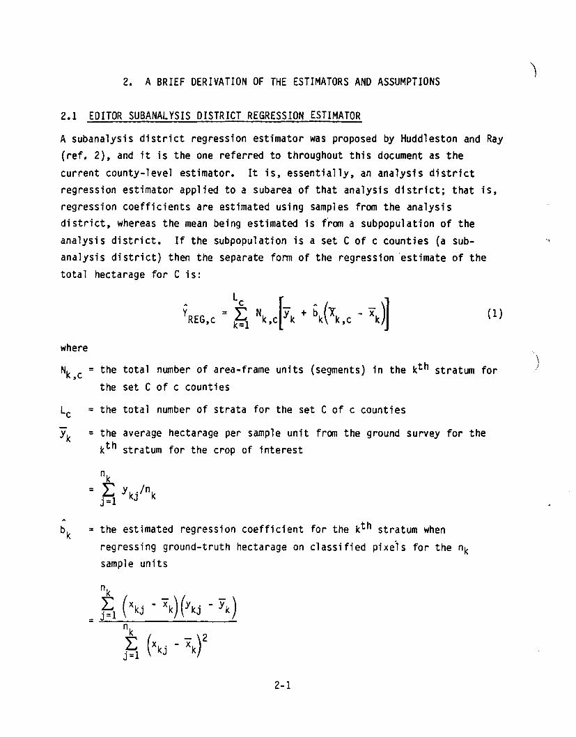
2.1 EDITOR SUBANALYSIS DISTRICT REGRESSION ESTIMATORA subanalysis district regression estimator was proposed by Huddleston and Ray(ref. 2), and it is the one referred to throughout this document as thecurrent county-level estimator. It is, essentially, an analysis districtregression estimator applied to a subarea of that analysis district; that is,regression coefficients are estimated using samples from the analysisdistrict, whereas the mean being estimated is from a subpopulation of theanalysis district. If the subpopulation is a set C of c counties (a sub- "analysis district) then the separate form of the regression estimate of thetotal hectarage for Cis:

(1)

whereNk,c = the total number of area-frame units (segments) in the kth stratum for

the set C of c counties)

= the total number of strata for the set C of c counties= the average hectarage per sample unit from the ground survey for the

kth stratum for the crop of interest

bk = the estimated regression coefficient for the kth stratum whenregressing ground-truth hectarage on classified pixels for the nksampl e uni ts

2-1

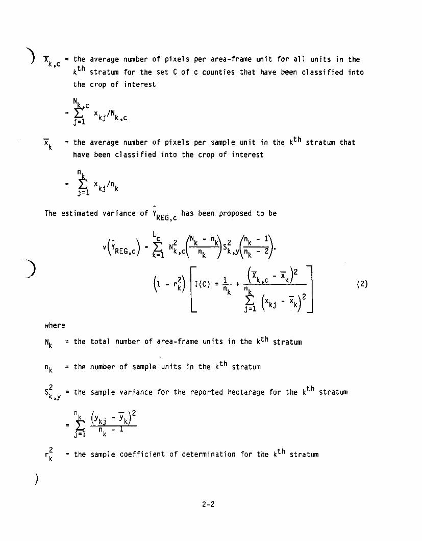
the average number of pixels per area-frame unit for all units in thekth stratum for the set C of c counties that have been classified intothe crop of interest

xk = the average number of pixels per sample unit in the kth stratum thathave been classified into the crop of interest

=

The estimated variance of YREG,c has been proposed to be

v(VREG,C)Lc

2 (\- n~s2 (nk - 1)= l: Nk,c nk - 2 •k=l k,y nk

)(1 - r~) +.L +

(Xk,c - xk)2I(C) nk nk

~ (Xk· - Xk)2J=l J

whereNk = the total number of area-frame units in the kth stratum

nk = the number of sample units in the kth stratum

S2 = the sample variance for the reported hectarage for the kth stratumk,y

n ( - )2= ± y kj - Y kj=l nk - 1

r; = the sample coefficient of determination for the kth stratum

)

2-2

(2)

I(C) = 1 if C is a subset of the regression domain= 0 if C is the entire regression domain

When I(C) = 1, the above variance formula is derived by treating the part of Ccontained in the kth stratum as a single (fictitious) segment in which thenumber of pixels classified as the crop of interest is Xk • This is,cequivalent to assuming that there is no variation at all for the actual seg-ments in C. If there is such variation, then it is believed that the varianceformula overestimates the variability of the subanalysis district regressionestimator. Comparing the empirical variances with those obtained from thevariance formula appears to substantiate this belief. For all of the majorcrops and for almost all of the minor crops, the empirical estimate ofvariance tends to be much closer to the formula variance for I(C) = 0 than forI(C) = 1, with most of the empirically observed values of I(C) falling in theinterval [0, .1]. These results are found in section 5.

2.2 THE CARDENAS FAMILY OF ESTIMATORSOne of the problems encountered in estimating crop hectarage in a subanalysisdistrict is that there may be few or no sample segments with which to obtainunbiased estimates of the mean hectarage per segment in the subanalysis dis-trict. Consider, for example, the six-county South Dakota area, and let Ckdenote one of the counties. If Ykh is the population mean hectarage per seg-ment of a crop in land-use stratum h and in Ck, then the total for county kwould be

(3)

where~ = denotes the summation over all strata in county kh e:C k

Mkh = the total number of segments in the hth stratum within county k

2-3

~ An unbiased estimate of the Ykh may not be possible if few sample segmentsbelong to Ck; however, the analysis district does presumably contain suffi-cient sample segments to estimate Yh, the population mean crop hectarage persegment in stratum h. Thus, if the assumption that Ykh = Yh were made, thetotal for county k would be estimated by

(4)

where

=.LNhV* 1: tihVih ' an unbiased estimate of Yhh nh i=1

tihthe hth stratumYih = 1: y. h .It.h ' the sample mean per segment of the area inj=1 1 J 1

within countytih = the number of segments in the sample of the hth stratum withi n county i

) nh = the number of counties in the sample of the hth stratum

Nh = the number of counties in the hth stratum.

Recognizing that the above assumption is not satisfied in general, Cardenas,Craig, and Blanchard (ref. 1) defined a family of county-level estimatorsusing the classified pixels in each county and stratum as the auxiliary data.The family of estimators (referred to herein as the Cardenas family of esti-mators) for the kth county is given by

(5)

whereXkh = the mean number of pixels classified as the crop in question for the hth

stratum within county kXh = the mean number of pixels classified as the crop in question for the hth

) stratum

2-4

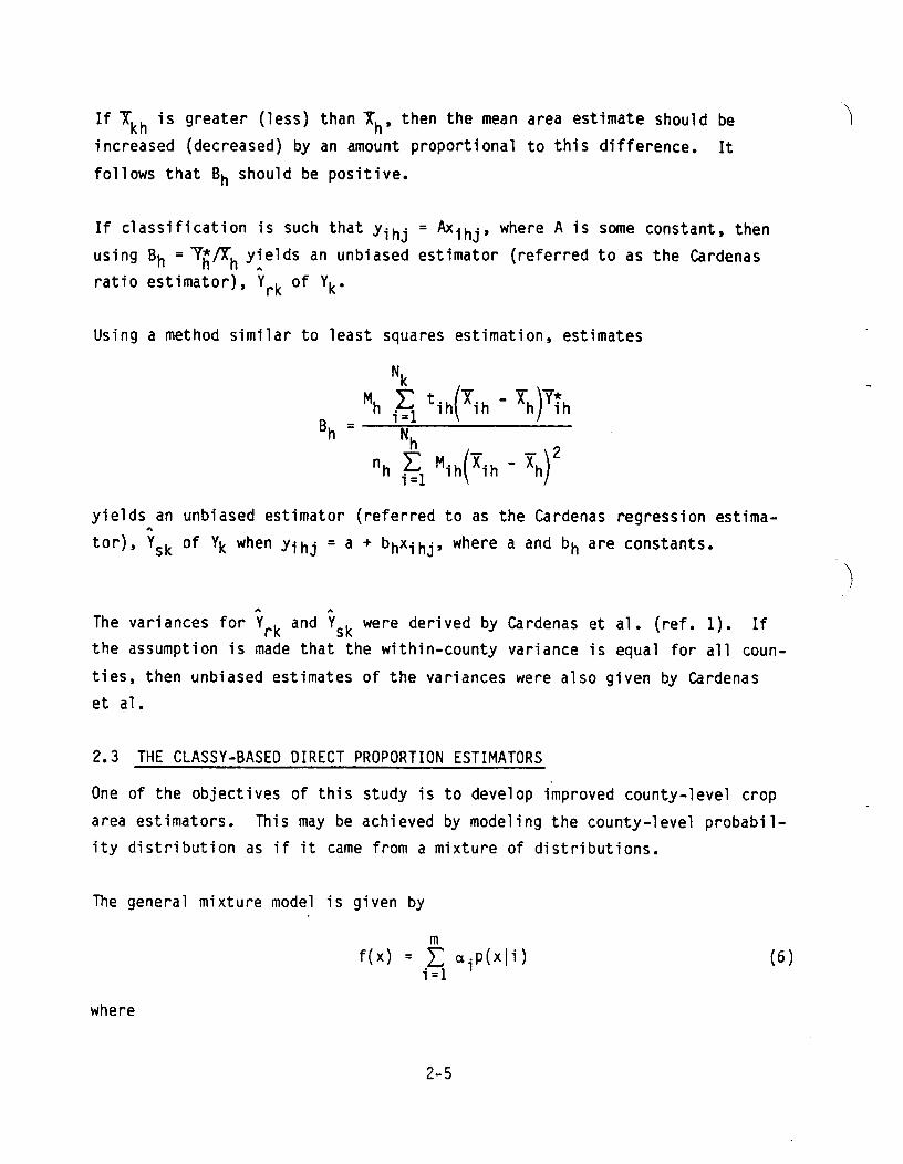
If Xkh is greater (less) than Xh, then the mean area estimate should beincreased (decreased) by an amount proportional to this difference. Itfollows that Bh should be positive.

If classification is such that Yihj = Axihj' where A is some constant, thenusing Bh = Yhtrh y!elds an unbiased estimator (referred to as the Cardenasratio estimator), Yrk of Yk•

Using a method similar to least squares estimation, estimates

yields an unbiased estimator (referred to as the Cardenas regression estima-.•.tor), Ysk of Yk when Yihj = a + bhXihj' where a and bh are constants •

.•. .•.The variances for Yrk and Ysk were derived by Cardenas et ale (ref. 1). Ifthe assumption is made that the within-county variance is equal for all coun-ties, then unbiased estimates of the variances were also given by Cardenaset a1•

2.3 THE CLASSY-BASED DIRECT PROPORTION ESTIMATORSOne of the objectives of this study is to develop improved county-level croparea estimators. This may be achieved by modeling the county-level probabil-ity distribution as if it came from a mixture of distributions.

The general mixture model is given bym

f(x) = L a.p(xli). 1 11=

where

2-5

(6 )

p{xji) =

a·1the probability density for distribution i

= the proportion of distribution i in the mixturem = the number of distributions in the mixturef{x) = the mixture probability density for a spectral value x

Applying the CLASSY clustering algorithm (ref. 3) to the unlabeled county-level data, it is possible to estimate m, p{xli), and ai for i = 1,···,m. Theproblem which remains is how to associate a crop label with each of the dis-tributions, p{xli). This distribution labeling problem is the subject of asignificant amount of ongoing research. Lennington and Terrell (ref. 4)described a maximum likelihood estimator for the proportion of a given distri-bution composed of a specific class. Chittineni (ref. 5) presented thismaximum likelihood result and a similar result based on a probability ofcorrect labeling criterion. Heydorn, Lennington, and Myers (ref. 6) presenteda least squares, or regression, approach to this same problem. In each ofthese approaches the model is

)lTk = t 8·k

a. + €i=1 1 1

wherelTk = the proportion of crop type k in the county of interest~k = a set of "fitting" coefficientsai = the mixture proportions described previously€ = error

(7)

)

Heydorn, Lennington, and Myers (ref. 6) have pointed out that this approachmay be considered a generalization of stratified proportion estimation.Chittineni (ref. 5) observed that if the 8ls are restricted to either 0 or 1(true distribution labeling), then the maximization problem may be solvedexactly for the case of two or three subcrop types using an exhaustive searchstrategy.

2-6

"-All of these techniques for estimating the 8ik coefficients require that a )small subset of labeled pixels be available. One way to select this subset oflabeled pixels is to choose pixels from only those segments within the countyof interest. This technique may not be feasible if the number of segments inthe county of interest is small. Therefore, it seems appropriate to choosepixels also from segments within the county and adjacent to the county.

Not all of the approaches to obtaining estimates of the 8ik were evaluated.The chosen candidates were the maximum likelihood approach and the leastsquares, or regression, approach, both of which will now be discussed in moredeta il•

2.3.1 MAXIMUM LIKELIHOOD APPROACHSuppose that the CLASSY clustering algorithm is applied to approximate themultivariate mixture density of the data in the county of interest. Thisresults in a set of multivariate normal densities, p(xli), i = l,···,m, and aset of prior probabilities, ai' i = l,···,m. Now, suppose that there is a setof data points, Xj' j = l,···,n, and let the random variable e be the classlabel which takes on values of i = l,···,c. The joint probability of observingdata point Xj associated with label e = i may then be formulated as follows.

mp(x.,e = i) = L a.P(x.,e = t Ii)J i=l 1 J

m= L a.P(e = tlx.,i)P(x./i) (8 )

i=1 1 J J

Assume that p(e = tIXj,i) = p(e = tli) = 8ti, which means that the labeledrandom variable e is conditionally independent of the observation Xj; i.e.,given that one is sampling from distribution i, no further information aboutthe class label is conveyed by knowing Xj.

2-7

Under this assumption, the proportion of class t may be estimated as

(9)

)

and ati may be interpreted as the proportion of distribution i that iscomposed of class t.

Now, a maximum likelihood approach may be used to estimate ati, assuming thatall ai and P{xjli) are given.

cGiven a random sample of N (= L Nt) 1abel ed data points from the county of

t=1interest, the likelihood function is

(10)

where x. , jt = 1, ···,Nt represents those data points labeled as coming fromJtclass t.

Under this mixture model, the likelihood function L may be written

c Nt mL = II II L a.at·p{x. Ii)t=1 jt=l i=1 1 1 Jt ( 11)

cTo maximize L subject to the constraints L ati = 1 for i = 1,"·,m is equiv-

t=1alent to maximizing the following function

t ~.(t a9, i - ~i=1 1 9,=1 I (12)

)where Tl., = 1, ·",m, is the Lagrange multipl ier.

1

2-8

aFMaximizing with respect to 6ti, a solution of ~ = 0 is given byti

where

(13)

(14)

Therefore, ati can be approximated using a fixed-point iteration scheme begin-ning with a . = 1 t = 1 ••• c i = 1,···,m. Once the solution of ao1' is

tl C' " , '"obtained, the proportion of class t can be estimated as

(15)

2.3.2 LEAST SQUARES APPROACHSuppose again that the CLASSY clustering algorithm has been applied to approx-imate the multivariate mixture density of the data in the county of interest.This results in a set of multivariate normal densities, p(xli), and priorprobabilities ai' i = 1, ···,m. The model considered in this case is aregression model where ati are just constants to be estimated, viz,

mp(e = tlx.) = I: at·p(i/x.) + g

J i=1 1 J

wherep(e = tlxj) = the posterior probability that Xj belongs to crop type tp(i IXj) = the posterior probability that Xj belongs to distribution i

= error

(16)

Now, the standard least squares techniques may be used to estimate ati• Thecriterion function to be minimized is

2-9

where

mK = IP{e =tlx.) - L a .P{ilx.)IFJ i=1 tl J

(17)

U-IIF ='V f{_)2dF, and F is the cumulative distribution of the mixture density_

To minimize K is equivalent to minimizing

2 m 2K = a p{e = tlx.) - L a oP{ilxo)uFJ i=1 t 1 J

j-~(e =1Ix.) - f. e .P(1Ix.02if. a.P(x.IJdX. (18)J i=1 tl Jj ~=1 1 J J J

Minimizing with respect to ati' the solution ism

a 0 = L: q·kE[p{e = tlxo)P{klx.)]t 1 k= 1 1 J J

where qik is the ikth element of the inverse of the matrixH = E[P{i IXj)P{klxj)].

;

Given a random sample of labeled data points and associated labels(xj,e = tj), j = 1,-" ,n, where tj € {l, ••• ,c}, ati ~an be estimated by

m ..• 1 nati = L qik n ?: lj/t(tJo)P{klxJ.)k=1 J=1

where

11ift=to_ J

o otherwi se= the ikth element of H-1 and the ikth element of H is

1 nn .L P{ilxJo)P{klxJo)J=l

2-10

(19)

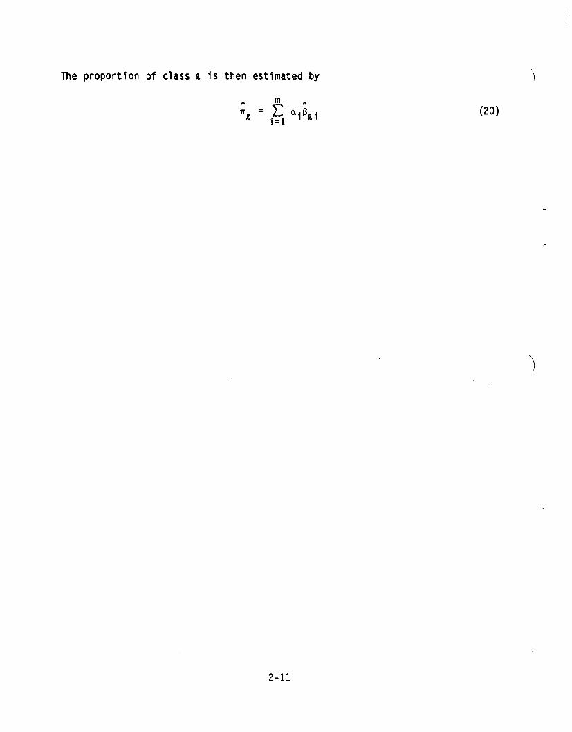
The proportion of class 1 is then estimated by

2-11

(20)

3. THE PREPROCESSING ALGORITHMS

3.1 XSTAR: AN ALGORITHM TO CORRECT LANDSAT DATA FOR THE EFFECTS OF HAZE ANDSUN ANGLEThe XSTAR preprocessing algorithm is based on the Environmental ResearchInstitute of Michigan (ERIM) radiative transfer model for an atmosphere withno absorption.

Letting primes denote a desired standard condition, the optical thickness foreach multispectral scanner (MSS) channel I is represented as follows:

where•L RI = the Rayleigh optical thickness in channel I

(21)

aIY' = the aerosol optical thickness in each channel so that y' is a scalarmeasuring the amount of haze in the atmosphere in a hypotheticalspectral band for which aI = 1

aI = a function of the channel, independent of atmospheric haze

For Landsat-2 data, channels 1 through 4,

,\i

1.26801.0445

g, =.9142.7734

(22)

The values for aI were calculated from the estimated Landsat in-band opticalthickness for an atmosphere with a horizontal visual range of 23 kilometers(14.38 miles), which is relatively clear.

Similarly, for an observed condition, the optical thickness is(23 )

3-1

However, the Rayleigh optical thickness is independent of atmospheric haze;so,

and (24 )

The change in optical thickness from the standardized condition to be observedis then measured by y.

If XI is the observed and Xi is the standardized Landsat radiance value inchannel I, and assuming that other variables in the radiative transfer equa-tion are restricted so that only atmospheric optical thickness is significant(ref. 8), a correction equation is obtained:

(25 )

In general, both Xi and P{aIA) are functions of scanner geometry, illuminationand viewing geometry, optical thickness, and the background albedo of thestandardized conditions.

Excluding the higher order terms, represented by the polynomial functionP{afY)'

aIYX' = e XI I

or (26 )

Then X* specifies a point, or an origin, in the signal space relative to whichthe remainder of the signal space expands or contracts according to the effectof each multiplicative factor. For a sun angle of 39°,

)

61.9X* = 66.2

83.233.9

3-2

(27)

To apply the XSTAR preprocessing algorithm to Landsat data, Y, a measurementof the amount of correction required, must be found. It is assumed thatLandsat data distributions lie in a two-dimensional hyperplane in four-dimensional data space and the hyperplane position shifts with atmospherichaze. The XSTAR algorithm uses the tasseled-cap yellowness direction y* as ameasure of the component of the shift, which is perpendicular to the usualorientation of the plane. For the standardized condition, the average signal

,.value measure in the Y direction is

y* = -11.2082 Landsat counts (28)

A value for y that will shift the mean :ignal value CfI) is calculated so thatthe mean corrected signal value in the Y direction will be Y*.

Y* -_ ~ ~ a IY U 6 X ( 1 a IY) x*J"Ye - -I + - e I I1=1 Uo(29 )

with un = cos 39° and Uo = the cosine of the sun angle at time of acquisition.

aIYIf e is expanded and third and higher order terms are ignored,

4 2 [u~a = L a -xI=1 I U 0 I

4 ~~ XiJY I (30)b = L aI -XI-1=1 Uo

4 L~'Jc = L -x IYI - y*1=1 Uo

Then -b [ nJ (31)Y"'a1-1--;TFor extremely hazy conditions, 1 - 2ac/b2 may be negative and the square root;s set to zero; i.e.,

Y = .:!a

3-3

3.2 ATCOR: AN ALGORITHM TO CORRECT LANDSAT DATA FOR THE EFFECTS OF HAZE, SUNANGLE, AND BACKGROUND REFLECTANCE

The ATCOR algorithm is designed to simulate the effects of target reflectancePI' sun angle e, haze level TH' and average reflectance of adjacent areas PIon the radiance of a target as measured by Landsat in a channel I, and tocorrect for them. ATCOR assumes that radiances measured by the sensor can bemodeled by

(32)

where LI is the response in band I and AI and BI are coefficients for channel Iwhich depend on VI' eO' and TH•

An atmospheric model was developed for use with ATCOR; the VandeHust methodwas then used to compute, for a range of wavelengths, the radiances gatheredby the MSS for a range of values for VI' eO' TH, and PI. These values arerepresented by a table in ATCOR.

) Generally, eO is known, but PI and TH are not.PI can be calculated from the table.

However, if TH is known, then

)

The ATCOR program estimates TH, computes VI' and interpolates using the tablesfor AI~I,eO,TH) and BI(~I,eO,TH) to find the correction coefficients whichcan be used to make the desired corrections.

The atmospheric model consists of two homogeneous layers: a Rayleigh scatteringmolecular layer on top and a Mie scattering haze layer next to the Earth1ssurface. Most haze is present in this region. The method used to determine thelevel of haze present actually estimates the total effect of all aerosols in theatmosphere and does not distinguish between haze and cirrus clouds. However,because the model assumes that this contribution is from haze particles in thelower atmosphere, the correction is less than optimal. Water vapor and othergaseous absorption are neglected.

3-4

The ATCOR program assumes that it is possible to obtain an estimate for the ~actual reflectance of the darkest pixels in a Landsat image and that the pres-ence of haze will brighten the corresponding measurement at the sensor. Theprocedure for obtaining this estimate is discussed in reference 7. Theatmospheric model indicates that the effect of haze is greatest in channel 1.The average channel 1 value for the darkest pixel in each scan line is computed(Xmin). The reflectance of the darkest target is known or is set to a defaultvalue. From these values, the haze level which causes such a change between theactual or default (darkest) reflectance and the observed ~in is interpolated inthe table. That value is the estimate for TH•

AI and BI may then be obtained from the table and the correction applied.

If primes denote the desired standard sun angle, haze level, and averagebackground reflectance, then:

(33)

where

lJ - cos 6.o -Xi is the new radiance value for pixel X, channel!.

3.3 MLEST: A DISTRIBUTION MATCHING ALGORITHMThe MLEST algorithm is a statistical approach to finding an affinetransformation of the form

\,;

Y = AX + B (34)

which transforms clusters of normal distributions in the MSS signal space froma training area in a manner which best describes the clustering of distribu-tions in a recognition area.

3-5

The objective of this approach is to model atmospheric and background effectsusing a maximum likelihood algorithm to develop a transformation matrix A anda vector B, in which the matrix A is not restricted to a diagonal matrix.This allows the estimated changes in a single MSS channel to be expressed as aweighted sum of the ensemble of channels rather than as a scalar transforma-tion of only the data in that particular channel. This transformation is ableto correct for haze differences and for any other affine transformationspresent in the data, regardless of origin. The primary advantages of MLESTover the XSTAR and ATCOR algorithms are that the nondiagonal terms of thetransformation are included, and it is not necessary to make assumptions aboutminimum haze pixels.

The following procedure is used to evaluate the performance of the MLESTalgorithm.1. Obtain unlabeled clustering statistics for a training area. The overall

probability density function for accomplishing this is

where

MP (XJo) = L: a. p (X . Ii)

i=1 1 J(35)

)

M is the number of clusters in the training area,Xj is the jth pixel in the training areaa. is the proportion of the ith distribution in the training area

1

2. Use these statistics and the MSS channel data from the recognition area asinputs to the MLEST algorithm. The MLEST algorithm estimates an affinetransformation of the training statistics and the a priori clusterprobabilities which maximize the likelihood function.

3. Transform labeled statistics from the training area using the computedaffine transformation:

3-6

..• A

J!iR = AlJ· + B-ITA A AI

L:iR= AI:. A1T

wherethe subscripts Rand T refer to the recognition and training areas,respectively •.•.A is the estimated transformation matri x..•B is the estimated transformation vectorlJ· is the mean vector for the ith distribution-1

L:. is the covariance matrix for the ith distribution1

4. Use the transformed and labeled statistics to classify and label thepixels in the recognition area.

3-7

(36)

4. EXPERIMENT DESIGN DESCRIPTION

4.1 INTRODUCTIONThe approach to be used was to estimate empirically the bias and variance ofthe estimator by repeated sampling. In order to implement this approach, itwas necessary to determi ne the appropri ate number of segments from the analy-sis district needed for training the classifier, that is, to determine thesize of a training group. In addition, the number of training groups to beused had to be determined, and, if possible, these training groups madepairwise disjoint. Each training group would be used in the following ways:1. A classifier would be trained using the segments in the training group.2. The segments in the training group would be classified.3. The regression coefficients for an estimator would be estimated using the

ground-truth hectares and the number of classified pixels in the traininggroup segments.

4. A given subanalysis district would be classified, and an estimate would beobtained of crop area in the subanalysis district, using the regressionestimator in number 3.

The estimates of crop area obtained from the training groups would be used tocalculate a sample estimate of variance and a mean estimate of crop area.The sample estimate of variance would be compared to the formula-obtainedvariance; and, as a measure of bias, the mean hectarage estimate would becompared to the direct expansion estimate, based only on the ground-truthsegment data from the subanalysis district being estimated.

There was some question about the sufficiency of the South Dakota data forestimating bias and variance using the repeated sampling method justdescribed. For comparison purposes, such a procedure should use repeatedindependent selections of segments for training; that is, the training groupsshould not overlap. A preliminary test study explored the issue of requiringtraining groups large enough for classification accuracy while at the same

4-1

\/

,time needing nonoverlapping training groups for the empirical estimation ofbias and variance and for the use of subsequent statistical tests. This studyis described in section 4.2.

4.2 FORMULATION OF GROUPS FOR TRAINING AND TESTINGGiven the requirements imposed on the training groups by the repeated samplingmethod, a preliminary study was made to determine the appropriate size of thetraining groups for reliably estimating the mean and variance of the estima-tor. Some problems were anticipated and are now described.

The 252 65-hectare (one-fourth-square-mile) segments were obtained by samplingwithin-soil strata instead of land-use strata. Resampling, which wasnecessary because some strata were oversampled, reduced the number ofavailable segments to 200. Ideally, a large number of independently selectedand nonoverlapping groups of segments should be used with repeated sampling todo the empirical estimation. Because classification was also carried out in

.) this study, each nonoverlapping group had to contain a sufficiently largenumber of segments to train the classifier. If the number of availablesegments is fixed, the number of segments within each nonoverlapping groupdecreases as the number of groups increases. Thus, if there were enoughnonoverlapping groups to do the empirical estimation, these groups might notcontain enough segments to adequately train the classifier. On the otherhand, if there were enough segments in each nonoverlapping group to do thetraining, there might not be enough groups to do the empirical estimation.Therefore, it was apparent that, in order to have enough segments in eachgroup to obtain acceptable classification performance and enough groups toconduct the empirical estimation of the variance, the use of overlappinggroups was unavoidable. The training groups were determined with theseconstraints in mind. The county-level estimators were based on the require-ments that a simple random sample of segments would be chosen within eachland-use stratum and that the CLASSY clustering algorithm assumes a simplerandom sample from the population; thus, each of the soil strata that was

4-2

oversampled was resampled so that the new sample size for each stratum wouldbe proportional to the area in that particular stratum. (Simple randomsampling of a population is nearly equivalent to stratified random samplingwith proportional allocation.) After resampling. 200 segments were left inthe six-county area. These 200 segments were used to train the classifier.which was to be used as a benchmark in evaluating any other classifiersobtained in the repeated sampling process.

Previous experience in the FY 19BO DC/LC project indicated that seventy-five65-hectare (one-fourth-square-mile) segments probably contained a sufficientnumber of pixels to train a classifier. Thus. the 200 segments were randomlypartitioned into B sets containing 25 segments each and were denotedSit i = It"""tB• The training groups were formed by combining three sets at atime so that the intersection of any two training groups would be at most oneset of 25 segmentst and each would be used in exactly three different traininggroups. The collection of training groups used in this study is as follows:

{SIUS2US3t SIUS4U~6. S2US4US7t S2US5USB'S3US4USSt S3US6USBt S5US6US7, SIUS7USB}

Some of the advantages of combining the partitions to obtain training groupsinstead of using simple random sampling are:1. The maximum number of overlapping segments in any two groups can be

controlled.2. Each segment is chosen the same number of times, whereas in simple random

sampling some segments may never be chosen and some could be chosen morethan the others.

Each of the training groups was used to train a classifier. Then the entiresix-county area was classified and county-level estimates were obtained. Thevariability of the eight classifiers was examined, and the performances werecompared with the benchmark of training on all 200 segments.

4-3

The criteria on which the collection of training groups was accepted were:1. Individual classification performances did not depart significantly from

t he benchmark.2. The number of groups was large enough to provide reliable empirical

estimation.

4.3 QUESTIONS ADDRESSED IN THE EVALUATION STUDIESThe evaluation study for the current county-level estimator addressed twoquestions.

First, when the value I(C) = 1 is used in the variance formula, the resultingnumber was believed to be an overestimate of the variability of the currentcounty-level estimator. Recall from section 2.1 that I(C) = 1 is used when-ever C is a proper subset of the regression domain and is equivalent toassuming that there is no variation at all for the segments in C (the county).If C is the entire regression domain, then I(C) = 0; and the estimator issimply the current analysis district regression estimator. Obtaining anempirical estimate of the variance and comparing it to the formula varianceusing different values for I(C) would be a means of examining the aboveassumption and also of estimating a more realistic value for I(C).

The second question was whether or not the current county-level estimator wasan unbiased estimator of the total crop hectarage for a county. To answerthis question decisively would require knowing the true crop hectarage for acounty, and this information was not available. Instead, the standard used

'"for comparison was the direct expansion estimator for the county, Y = N x y,where N is the total number of possible segments in the county and y is thesample mean crop hectarage per segment for the given county.

The particular alternative county-level estimators that were evaluated were ofinterest because of the approaches that were taken in hectarage estimation atthe subanalysis district level. The Cardenas family of estimators compares

) the average number of crop pixels per segment in a given stratllTlto the

4-4

average number of crop pixels per segment in the given county in that stratumand adjusts the mean area estimate by an amount proportional to thisdifference. Therefore, it was desirable to compare the performance of two ofthe members of this family to the current county-level estimator as well as tocompare the performances of these two Cardenas estimators. In addition, theonly variance formula available for this family makes the assumption that, forall counties, the within-county variances are equal. To compare the empiricalestimate of variance to the formula variance as an indication of the validityof this assumption was also a desirable objective.

The two direct proportion estimators offered the possibility of estimatingcrop hectarage in a county using only the county Landsat data and relativelyfew ground-truth pixels. Another advantage was that the classification ofeach pixel is not done directly as is necessary for the regression type esti-mators. For making comparisons, however, this was also a disadvantage in thisstudy. For each county, one estimate of a crop proportion was obtained ratherthan eight estimates using eight classifier training groups. Questions re-garding the size of bias and variance were answered by using the proportionsand variances generated by the simple random sample approach (section 5.3) asthe standard.

4.4 PREPROCESSINGThe objective of the preprocessing study was to see if candidate preprocessingalgorithms applied to analysis district Landsat imagery have the capability forimproving crop area estimates at the county level when few (or no) trainingsegments are available from that county. Three preprocessing algorithms werechosen for study based on results of the Large Area Crop Inventory Experiment:XSTAR, ATCOR, and MLEST (see section 3). The XSTAR and ATCOR algorithms arehaze-correction models which transform the analysis district and the county tobe estimated to correct for the presence of haze and/or background effects andto make them look spectrally similar to the classifier. The MLEST algorithmtakes distributions present in the analysis district and estimates an affineshift correction which matches them to distributions from the county. A

4-5

)

transformation is obtained which may then be used on the statistics in theclassifier before classifying the county.

Ideally, sample segment data chosen from the analysis district (a six-countyarea) would be used as the training set on which to develop the regressionestimator, and an entire county would be used as the test area. However,ground truth was available only for sample segments in the county. In thisstudy, we tested whether preprocessing improves the estimates for a samplefrom a county, rather than whether it improves an actual county estimate.

In order to address the worst possible case, two test areas (sample segmentsfrom Beadle and Kingsbury counties, South Dakota) that did not overlap thetraining set were chosen. This effort not to duplicate sample segments fromthe training set in the county was made for two reasons: First, to achievedistinct test and training groups for the F-test and the Hotelling T2 test;and, second, to provide the IIworstllcase, where no sample segments from thearea of interest were available for tra~~ing. This selection also fulfilledthe requirement that sample segments from surrounding areas be available fortraining; the surrounding segments in this case were other training groupsegments that were i~ Beadle and/or Kingsbury Counties.

After estimates for the county samples were obtained by the USDA EDITOR systemand by the USDA EDITOR with MLEST, ATCOR, and XSTAR preprocessing, a compari-son was made to see which method produced estimates closer to the true ground-truth proportions.

The purpose was to ascertain if one of the preprocessing methods had in someway made the regression estimator, which was developed over the analysisdistrict, appropriate and accurate at the county level.

4.5 STATISTICAL EVALUATION APPROACHIt was apparent from the preliminary analysis that the overlap among sometraining groups would vitiate any statistical tests requiring that assumptionsof independence of random variables be satisfied. Tnis was accepted as a

4-6

necessary flaw in order to have enough training groups with enough segments ineach group to adequately train the classifier.

In evaluating the conjecture that the formula for the variance of the currentsubanalysis district regression estimator overestimates the variability ofthis estimator if I(C) = 1 is used, the following approach was taken: Thearithmetic means over the eight training groups were plotted against thecorresponding values of I(C) = 0 and I(C) = 1 for each crop. The linecontaining these two points expresses the linear relationship existing between,.I(C~ and the variance of Yc' as is evident from the formula for the varianceof Y. This line can be used to approximate the value of I(C) associated withcthe empirical estimate of variance.

The Behrens-Fisher test was used to investigate the bias of the currentcounty-level estimator. Whenever a sample of segments is randomly selectedfrom a county, the direct expansion estimator N x y is an unbiased estimatorfor the total county hectarage of a given crop. Likewise, each individual Yi ']is unbiased for the mean number of hectares per segment. Similarly, if thecurrent county-level estimator is unbiased for the total county hectarage of agiven crop, then this estimator divided by the number of segments in thecounty (N) is unbiased for the mean number of hectares per segment for a givencrop. The Behrens-Fisher test indicates whether the current county-levelestimator, when divided by N, systematically overestimates or underestimatesthe mean number of hectares per segment.

For the Cardenas ratio and regression estimators, the proportions of each cropin each county, as well as a "coefficient of variation" for each crop, arepresented in tables. These figures are calculated for each training group.This "coefficient of variation" is, for each county, the ratio of the squareroot of formula variance for the crop divided by the average number ofhectares of the crop. In addition, a sample coefficient of variation wasobtained using the estimates of a crop from the eight training groups assamples. These summary statistics for each estimator are presented by crop.

4-7

) The sample variances of the Cardenas estimators were compared, and the samplevariance of each Cardenas estimator was compared to the sample variance of thecurrent county-level regression estimator using an F-test. This was doneknowing that the independence assumptions were not satisfied. Indeed, notonly did some of the training groups overlap, but also all three estimatorshave the same y-variable, namely the ground truth hectarage per segment.However, it was believed that a comparison of the sample variances wouldindicate whether or not they were significantly different.

The Behrens-Fisher t-test described previously was the test for bias of theCardenas ratio and regression estimators.

The bias and the mean squared error (MSE) of the direct proportion estimatorswere calculated and recorded as summary statistics. Recall that the procedureis to cluster a county and obtain proportions, Qi' of each distribution in themixture model. Then, 500 labeled pixels are chosen randomly from segments

.) within the county to estimate St ' or the proportion of crop R. in distribu-i c

r tion 1. The proportion of crop 1., 1T~, is L Q.B~ , where c is the number ofA. • 1 1 A..

1= 1di stributions present. In addition, the crop proportions taken from the 500pixels are computed to obtain a third estimate, called the simple random sampleestimate. This procedure is repeated 50 times, each time choosing 500 labeledpixels randomly from the segments within the county. The average number oflabeled pixels available in each county is about 6700, a large enough numberthat the 50 repetitions can be considered independent. The proportion of eachcrop, determined using all the labeled pixels in a county, is considered thetrue proportion of that crop. In order to estimate the bias, the 50 estimatesare averaged and the mean compared to the proportion in the labeled pixels.The MSE is the sample variance of the 50 proportion estimates. An F-ratio iscomputed for each of the direct proportion estimators. This is the ratio ofthe sample variance of the direct proportion estimator to the sample varianceof the simple random sample estimates over the 50 repetitions. Independenceproblems are again present, since each of the three estimates (maximumlikelihood, least squares, and simple random sample estimates) is obtained overthe same set of 500 pixels.

4-8

4.6 EVALUATION OF PREPROCESSORSThe comparison of the performance of each preprocessor with the USDA EDITOR wasdone using the Hotelling T2 test, which compares the mean difference betweenground truth and the regression estimate per segment for both methods.Accepting the null hypothesis would indicate that there is no significantdifference between estimates produced by the two methods.

There remains some question as to whether the regression equation developedfrom the analysis district should be used on the county in evaluating theperformance of the MLEST algorithm, since a new (transformed) classifier isused on that county. Although an improvement in classification was obtainedusing the MLEST algorithm on the county data, a corresponding improvement inestimation might not occur using the regression lines developed on the analysisdistrict if these regression lines are not appropriate for the county. So inaddition to the Hotelling T2 test for the other preprocessors, two other testswere made: one to compare regression estimators for the USDA EDITOR and MLEST,which were developed on the county; and one to compare estimates from the USDA )EDITOR using the training regression lines and MLEST using the countyregression lines. This issue is discussed in further detail in section 5,Study Results.

If the results of the Hotelling T2 test show that one or more of the preproc-essing procedures produce estimates that are not significantly different fromthose produced by the USDA EDITOR alone, it is necessary to examine the meanvector to determine if the results of the preprocessing procedure are better,worse, or mixed. If the estimates using the preprocessor are closer to groundtruth for every crop than those of the EDITOR alone, then the results using thepreprocessing procedure are considered better; if they are further from groundtruth for every crop than those of the EDITOR alone, the results using thepreprocessing procedure are considered worse. If the estimates using thepreprocessor are closer to ground truth for some crops and further for others,it may be concluded that one procedure is not better than the other.

4-9

~)

)

In order to attempt to detect the presence or absence of haze or other differ-ences between the test and training areas, a two-sided F-test for homogeneityof variances and an F-test for equality of analysis district and countyregression lines is done for each crop. These tests are discussed in moredetail in section 5.

4-10

5. STUDY RESULTS

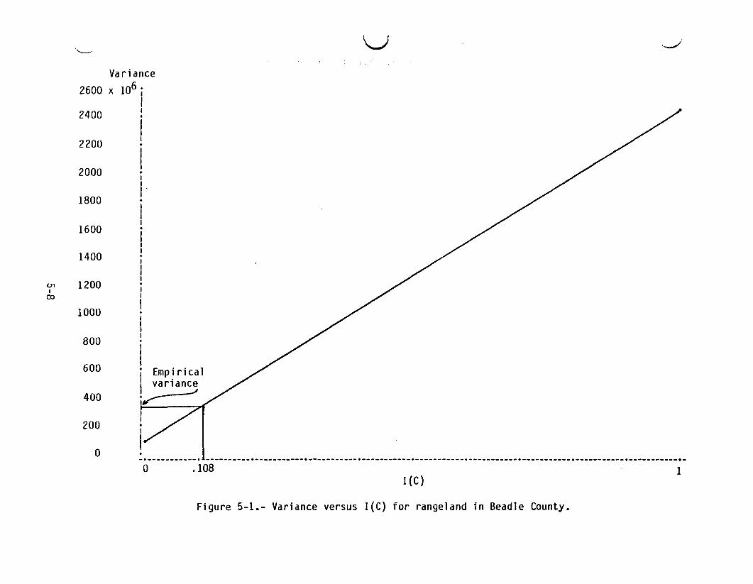
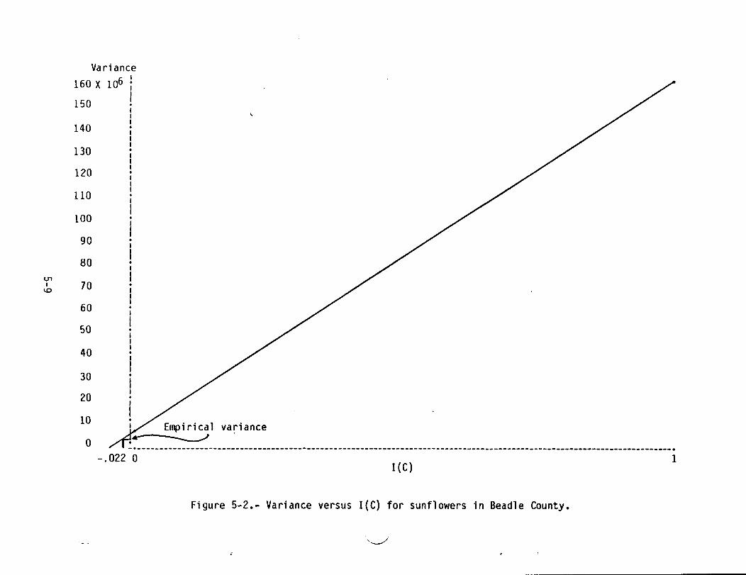
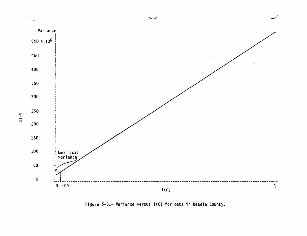
5.1 CURRENT SUBANALYSIS DISTRICT REGRESSION ESTIMATOR5.1.1 EXPLANATION OF GRAPHS AND TABLESFigures 5-1 through 5-9 contain plots of variance versus I(C) for the currentcounty regression estimator. For each crop, the formula variance usingI(C) = 1 is computed for each training group, and an average is obtained.Similarly, the formula variance using I(C) = 0 is computed for each traininggroup, and an average is obtained. These two numbers determine the lineassociated with each crop. The empirical estimate of variance is then usedwith this linear relationship to produce an empirical estimate of I(C).

Although these plots have been produced for only one county, other dataexhibited later provide a similar result: for the majority of crops in eachcounty, the empirically estimated values of I(C) are around zero. This tendsto confirm the statement that the formula variance provides an estimate whichgreatly overestimates the variance of the current county-level estimator.

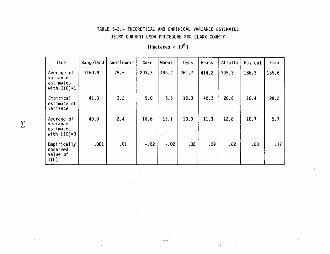
5.1.2 THEORETICAL AND EMPIRICAL VARIANCE ~STIMATES BY COUNTYTables 5-1 through 5-6 present the preceding graphical results quantitativelyby county. The averages across training groups of the theoretical andempirical variance estimates for each crop are given. The empirically observedvalue of I(C) is also given, and it was determined by observing that in theformula I(C) is linearly related to the variance estimate. The averages of thevariance estimates with I(C) = 1 and also with I(C) = 0 provide two pointsdetermining the line representing this linear relationship. By using this factand the empirical estimate of variance, one can obtain a corresponding value ofI(C). For the majority of crops in each county, these values of I(C) are closeto zero.

5-1

~I;

111IN

TABLE 5-1.- THEORETICAL AND EMPIRICAL VARIANCE ESTIMATESUSING CURRENT USDA PROCEDURE FOR BEADLE COUNTY

[Hectares x 106]

Item Rangeland Sunflowers Corn Wheat Oats Grass Alfalfa Hay cut FlaxAverage of 2428.5 160.0 580.4 1034.5 532.3 969.5 680.3 322.6 285.7va rianceestimateswith I(C)=lEmpi rica 1 332.9 1.1 4.2 131.9 25.9 60.0 76.7 36.8 5.2estimate ofvarianceAverage of 79.9 4.5 19.5 32.5 15.8 25.6 21. 7 14.4 9.1varianceestimateswith I(C)=OEmpirically .11 -.02 -.03 .10 .02 .04 .08 .07 -.01observedvalue ofI(C)

lT1IW

TABLE 5-2.- THEORETICAL AND EMPIRICAL VARIANCE ESTIMATESUSING CURRENT USDA PROCEDURE FOR CLARK COUNTY

[Hectares x 106]

Item Rangeland Sunflowers Corn Wheat Oats Grass Alfalfa Hay cut FlaxAverage of 1160.9 75.5 293.3 496.2 261.7 414.2 335.3 186.3 135.6varianceestimateswith I(C)=lEmpi rica 1 41.3 3.2 5.0 5.5 16.0 46.3 20.6 16.4 28.2estimate ofva rianceAverage of 40.0 2.4 10.6 15.1 10.0 11.3 12.8 10.7 5.7varianceestimateswith I(C)=OEmpirically .001 .01 -.02 -.02 .02 .09 .02 .03 .17observedvalue ofI(C)

U1I~

\"_,Il

TABLE 5-3.- THEORETICAL AND EMPIRICAL VARIANCE ESTIMATESUSING CURRENT USDA PROCEDURE FOR CODINGTON COUNTY

[Hectares x 106]

Item Rangeland Sunflowers Corn Wheat Oats Grass Alfalfa Hay cut FlaxAverage of 504.5 32.5 130.5 216.7 116.9 166.0 148.6 87.9 57.9varianceestimateswith I(C)=1Empi rica1 48.1 .7 5.1 5.4 31.8 26.3 7.0 5.5 22.3estimate ofvarianceAverage of 20.5 1.1 5.1 7.0 6.7 4.7 6.3 5.9 3.0varianceestimateswith I(C)=OEmpi rica11y .06 -.01 0.0 -.008 .23 .13 .005 -.006 .35observedvalue ofI(C)

U1I

U1

TABLE 5-4.- THEORETICAL AND EMPIRICAL VARIANCE ESTIMATESUSING CURRENT USDA PROCEDURE FOR HAMLIN COUNTY

[Hectares x 106]

Item Rangeland Sunflowers Corn Wheat Oats Grass Alfalfa Hay cut FlaxAverage of 404.6 30.7 107.3 187.7 94.9 117.8 131.1 69.9 40.6varianceestimateswith I(C)=1Empirical 18.9 0.1 7.5 3.2 29.2 7.9 7.1 2.3 11.8estimate ofvarianceAverage of 17.5 1.1 5.6 6.4 3.6 3.5 5.5 2.5 2.1varianceestimates .'

with I(C)=OEmpi rical1Y .004 -.03 .02 -.02 .28 .04 .01 -.003 .25observedvalue ofI(C)

U1I

0"1

I\JTABLE 5-5.- THEORETICAL AND EMPIRICAL VARIANCE ESTIMATES

USING CURRENT USDA PROCEDURE FOR KINGSBURY COUNTY[Hectares x 106]

Item Range 1and Sunflowers Corn Wheat Oats Grass Alfalfa Hay cut FlaxAverage of 1522.4 100.8 349.3 638.5 327.7 663.1 412.2 175.4 187.2va rianceestimateswith I(C)=lEmpirical 50.0 0.6 13.8 15.6 10.1 17.0 19.7 2.6 77.0estimate ofvarianceAverage of 44.0 2.7 11.0 17.1 9.1 16.8 11.2 4.8 7.4varianceestimateswith I(C)=OEmpirically .004 -.02 .01 -.002 .003 0.0 .02 -.01 .39observedva 1ue ofI(C)

U1I'-J

TABLE 5-6.- THEORETICAL AND EMPIRICAL VARIANCE ESTIMATESUSING CURRENT USDA PROCEDURE FOR SPINK COUNTY

[Hectares x 106]

Item Rangeland Sunflowers Corn Wheat Oats Grass Alfalfa Hay cut FlaxAverage of 3058.8 213.1 756.9 1364.9 693.2 1109.8 923.8 421. 5 328.9varianceestimateswit h I(C)=1Empirical 209.4 65.2 17.3 115.7 64.1 35.5 276.4 61.6 24.2estimate ofvarianceAverage of 89.6 11.8 24.8 42.8 21.6 31.2 36.2 22.3 9.9varianceestimateswith I(C)=OEmpi rica lly .04 .27 -.010 .05 .06 .004 .27 .1 .04observedvalue ofI(C)

'---' V ,-/

Va riance2600 x 106 j

I2400 I

•II

2200 I•I

2000 I•II

1800 I'•IIII1600 •III

1400 I·III

1200 IU1 •I I

OJ I

1000 I

800

600

400

200

a -+ t ----- + t.- + + ----.--- + + + + •

a . 108I(C)

Figure 5-1.- Variance versus I(C) for rangeland in Beadle County.

1

-.------------------------------------.-----------------------------------------------------------------------------------.

Variance160 X 106 t150 I·I

II140 •III130 •II

120 I·II

110 I·II100 ·II90 •I

80 I•I

U1 II 70 •

\.0 II

60 I•I

50 I•II

40 I•III30 •I

20 I•J

10 Ivariance

0-.022 0

I(C)1

Figure 5-2.- Variance versus I(C) for sunflowers in Beadle County.

o -+----------------------------.---------.---------------------------------------------------------------------------------.- . 027 0 1

I (C)

I,'-"

J

--..../

~

Vari ance650 X 106 i

II

600 I•I

550 I•I500 •II

450 I•III

400 I•II

I350 •I

U1 300 I•I I•.....a I

250 I•II

200 I•III150 ·II

100 I•

50 Empiricalvariance

J

Figure 5-3.- Variance versus I(C) for corn in Beadle County.

-t ------- + + • + -----.------ + + + +_

Vari ance1300 X 106 •

I1200 I·I

tI

1100 I•II

1000 t•II

900 I•I

800 I•I700 •II

600 IU'1 •

II I•..... I•..... 500 ·II

400 I•

300 Empirical200

100

0o .099

I(C)

Figure 5-4.- Variance versus I(C) for wheat in Beadle County.

/

1

~i ..J

VarianceiI

500 X 106 I·II

450 I•III

400 I•I

II350 +

III

300 I+III

I250 •U1 II•.....

IN 200

150 +I

II

100 Ii EmpiricalI vari ance

50~

0-+- ---------+-----------+-----------+-----------+-----------+-----------+-----------+-----------+--.--------+-----------+-o .019

I(C)

Figure 5-5.- Variance versus I(C) for oats in Beadle County.

1

Variance1300 X 106 i

III•1200

1100

1000

900

800

700U1 600I•.....w

500

400

300

200

100

0

•I

I•II·II•IIII•I

I•III Empiricali variance

!~-+--- -------+-----------+-----------+-----------+-----------.-----------.-----------.----------~.-----------.-----------+-o . 036

I(C}

Figure 5-6.- Variance versus I(C} for grass in Beadle County.

1

VarianceI

800 X 106 i750 !I

I

700 !I

650 !

600 !I•II•

550500450400

(J1 350I~.po

300250200150100500

u

-+--------- -~-----------.-----------.-----------.-----------.-----------+-----------+-----------.-----------+-----------+-o .083

I(C)

Figure 5-7.- Variance versus I(C} for alfalfa in Beadle County.

1

•-+-------- --+---.-------+-------.---+-----------+-----------.-----------+-----------+-----------+-----------+-----------+-

300

275

250

225

200

175

c.n 150,•......c.n

125

100

75

50

25

0

Variance325 X 106 i

II·III•IIII•III .•II•III•III•III•

o

Empirical

.073I(C)

Figure 5-8.- Variance versus I(C) for hay cut in Beadle County.

1

I I\

\..-1'----Variance

325 X 106jI

300 I•I

275 I•II

250 I·I225 I200

175 •III

lTl 150 I•I I~ I71 I125 •

II

100 I•III

75 I•III

50 I•

25o _. •

-.014 0 1. I (C)

Figure 5-9.- Variance versus I(C) for flax in Beadle County.

5.1.3 BEHRENS-FISHER TESTTable 5-7 contains the results of the Behrens-Fisher test described in sec-tion 4.5. This test is used as a guide in assessing the bias of the currentcounty-level estimator. The corresponding confidence intervals for theestimated biases are in table 5-8.

This test, a significance test for the difference between the means of twonormal populations, assumes that the two population variances are not thesame. For a fixed crop and county, the eight estimates of hectarage associ-ated with the eight training groups are considered as eight observations of arandom variable YI•

For the same crop and county, the n sample segments of the 200 that fall inthat county can each be thought of as providing an estimate of the mean hec-tarage per segment of that crop. By multiplying each of these n numbers bythe total possible segments in the county, n estimates of the hectarage of thecrop are obtained. Treating these as n observations of a random variable Y2'this two-sample test can then be applied to test for the equality of meansassociated with the random variables YI and Y2• The following should be keptin mind in interpreting the test results: First, the eight observations of YIare regression estimates based on means from training groups, some of whichoverlap; and second, the n observations of Y2 arise from individual segmentsand thus produce a large sample variance. This variance will occur as part ofthe denominator in the test statistic, and it will likely produce a numberwhich will fall within the interval determined by the critical values. Thiswould imply that the hypothesis of equal means would not be rejected as oftenas might be expected, given that the efficacy of Y2 as an estimator of thetrue population mean is suspect.

The other possibility for estimating the true mean was to use the segmentsfalling within a county to obtain the direct expansion estimate of the truemean. This number would then be a constant C against which the mean from thedistribution of VI could be tested for equality. The difficulty with thispossibility is that C is treated as the true mean, when in reality, it is only

5-17

\)

U1I•.....

ex>

· I''--''TABLE 5-7.- BEHRENS-FISHER T-TEST OF MEAN ESTIMATES*

[n = • 05]

1 : Behrens-FisherCounty statistic Rangeland Sunflowers Corn Wheat Oats Grass Alfalfa Hay cut Flax

2: Critical values1 -1.50 ** -1.60 t5•52 -1.47 t2.77 -1.12 -1.24 **

Beadle 2 ±2.05 ** ±2.02 ±2.14 ±2.03 ±2.14 ±2.06 ±2.03 **1 -1.20 -0.81 1.07 -1.26 t3•58 -.34 .72 -.55 1.87

C1ark 2 ±2.04 ±2.03 ±2.03 ±2.03 ±2.06 ±2.06 ±2.06 ±2.05 ±2. 111 .63 -.08 -.19 1.08 .57 -1.49 1.45 ** .10

Codington 2 ±2.07 ±2.05 ±2.06 ±2.06 ±2.09 ±2.07 ±2.07 ** ±2.071 -1.80 ** t2.31 -.27 -1.52 t2•95 1.83 -.43 .59

Hamlin 2 2.11 ** ±2.ll ±2.10 ±2.12 ±2.16 ±2.12 ±2.12 t2.121 .20 -1.19 .08 -.87 t2.19 -1.46 .45 t3•60 .37

Kingsbury 2 ±2.05 ±2.04 ±2.05 ±2.05 ±2.07 ±2.05 ±2.07 ±2. 19 t2.141 .73 -.55 -1.21 -.83 .52 .57 .24 .62 .29

Spink 2 ±2.04 ±2.03 ±2.01 ±2.03 ±2.10 ±2.04 ±2.13 ±2.08 ±2. 08*The hypothesis is that the population mean of the current county-level estimator equals the populationmean of the direct expansion estimator.

tHypothesis rejected.**No crop present.

U1I~

\.0

TA8LE 5-~.- CONFlUENCE INTERVAL FOR ESTIMATED BIAS: CURRENT REGRESSION ESTIMATOR[95% confidence]

County Rangeland Sunflowers Corn Wheat Oats Grass Alfal fa Hay cut Flax

-6.275 -3.015 7.368 -2.625 2.574 -2.065 -3.075Beadle±8.573 ±3.815 ±2.861 ±3.627 ±l.987 ±3.788 ±5.0ll-4.867 -1.770 2.369 -2.879 4.067 -.739 1.024 -.729 1.808

Clark±8.233 ±4.432 ±4.487 ±4.642 ±2.346 ±4.423 ±2.922 ±2.723 ±2.034

2.641 -.090 -.466 1.777 1.255 -4.480 2.218 .294Codington

±~.607 ±2.420 t4.968 t3.407 t4.568 ±6.225 ±3.161 t6.264-9.222 8.533 -.682 -5.621 2.887 2.753 -.404 1.277

Hamlint10.772 ±7.792 ±5.403 ±7.817 ±2.119 ±3.196 t2.002 ±4.568

.809 -1.649 .267 -2.671 2.619 -4.376 .701 .928 .632Kingsbury

±8.246 t2.~25 ±6.915 ±6.300 ±2.474 ±6.137 ±3.234 t.564 ±3.6832.311 -1.280 -2.344 -2.288 .531 .820 .431 .718 .195Spink

±6.474 t4.714 t3.907 t5.594 ±2.147 ±2.918 ±3.891 t2.419 t1.427

)

an unbiased estimate of that mean, and it has a considerable amount ofvariance associated with it.

A decision to use the two-sample test was made, and, insofar as the mean of Y2can be considered the true population mean, the test results indicate thatthere is not enough statistical evidence to show that Y1, the current county-level estimator, is biased.

5.1.4 ESTIMATION RESULTS FOR SOIL STRATUM 4The current subanalysis district estimator was used to obtain crop hectarageestimates for soil stratum 4 for each of the eight training groups. (TheCardenas estimators were not evaluated on soil stratum 4 because their userequires knowing all of the land use stratum and soil stratum intersectionmeans, which were not available.) In an analysis similar to that which wasconducted for the six counties, an empirically derived value for I(C) wascalculated. These results are shown in table 5-9. Again, the empiricallyobserved values of I(C) cluster close to 0, with hay cut being the onlyexception. This gives additional credence to the conjecture that the varianceformula with I(C) = 1 produces overestimates.

The Behrens-Fisher test described in section 5.1.3 was used to ascertain ifthe current estimator produced biased crop hectarage estimates on soilstratum 4. Table 5-10 gives the results of the Behrens-Fisher tests. No non-zero ground truth was present for flax or grass in the sample of 20 segmentsfrom soil stratum 4. Of the remaining seven crops, there was not enough sta-tistical evidence to reject the null hypothesis of equal means. (A signifi-cant outcome for a crop would imply that the estimate for that crop is biased.)

5.2 RESULTS OF THE CARDENAS REGRESSION AND CARDENAS RATIO ESTIMATIONPROCEDURES

5.2.1 COUNTY CROP PROPORTION AND COEFFICIENTS OF VARIATIONTables 5-11 through 5-19 give, by crop, the proportion estimates and the"coefficients of variation" that were obtained for each training group for

)

5-20

<.nINI-'

TABLE 5-9.- THEORETICAL AND EMPIRICAL VARIANCE ESTIMATESUSING CURRENT USDA PROCEDURE FOR SOIL STRATUM 4

[Hectares x 104]

Item Rangeland Sunflowers Corn Wheat Oats Grass Alfalfa Hay cut FlaxAverage ofva rianceestimateswith I(C)=l 329.8 23.0 90.0 159.0 79.9 79.8 112.3 54.5 27.7Empiricalestimate ofvariance 59.7 .3 4.8 16.1 2.7 2.0 1.1 36.1 .8Average ofvarianceestimateswit h I(C)=0 14.5 .9 3.2 5.8 3.1 2.8 3.9 2.4 1.0Empiricallyobservedvalue ofI(C) .143 -.029 .018 .067 -.006 -.010 -•027 .646 -.010

)

TABLE 5-10.- BEHRENS-FISHER TEST OF MEAN ESTIMATES FOR SOIL STRATUM 4*[a = 0.5]

Crop Statistic Critical Confidence interval Relativevalue for estimated bias bias

Rangeland -0.408 ±2. 116 -2. 134 ± 11.060 -0.088Sunflowers -.947 ±2.094 -1.600 ± 3.539 -.948Corn -1.434 ±2.096 -6.019 ± 8.800 -.456Wheat 1.749 ±2.1l3 5.096 ± 6.157 1.007Oats -.618 ±2.104 -1. 009 ± 3.433 -.350Grass tAlfa1 fa -.420 ±2.099 -.580 ± 2.902 -.181Hay cut .309 ±2.159 .740 ± 5.161 -.202Flax t

*The hypothesis is that the population mean of the Huddleston-Ray subanalysisdistrict estimator equals the population mean of the direct expansionestimator.

tNo crop present in sample from soil stratum 4.

5-22

TABLE 5-11. - COUNTY CROP PROPORTION AND COEFfI CIENTS OF VARIATIONS FOR CARDENAS~EGRESSION ESTIMATOR AND RATIO ESTIMATOR FOR RANGELAND

(a) Cardenas regression estimator

r.r ,IIN , '( (,111 lJ140 (q It\ (,~••I b~'fi (,J4 '> (jjlJll I,~o I Mt:."!~P,WPO~ T ION CI(OP >iECrAI(t:.~lif{. Tbkl S C. v.

11",t.lll" II.\hM II. '.'l? rl.Bt> o.~().., II.1 11 U.JJ4 ,I. Uh'l U.III1/) ().~47 1~IU!ll.~"'tl II. ,l,h 11.',79 II.lli o. 2~ I 11.""0 II.J~b 11.4'-1,) II•.?b':> o.bol 27J.1'i~1'1~'I(LAH •... II.".~4 II .11.1) 1l.2..•R 0.~41 II.Zc..;~ 0.222 0.3~4 11.301 0.tt>8 6061614tl7114 U.lt2 o.~JJ II.1;'>1 11.121. II.140 O. l"~ o. I.,•• 1).IMb 0.1 bO 11331/94,.,3.JoCIIIlI"'",(IN O. Ibll \J.-it I (J • .?i9 o.~~~ n.3~9 0.11'1 11.20) 11.,1] 0.l74 46114lh~l~b 0.15" O.SH 0.171 1I.IH2 II.1 11 0.on7 00113 11.4'1, 0.0;11 S60o~3 46.84~\M1LI'~ 0.1.' ] II. IIJj o·rd 0.2')1 ll.240 U.llb~ (l·I'Jl ll.jOrj 0.)11 l3 9'~AIllIlJu O.3~~ U.14'1 II. 6~ 0.411 fl.5uo O. b1~ 0.3tl~ U.4117 0.:J1~ 1189 4011.04/< 1")(,S'ill"'Y 0.;>11>1 11.111 0.141 U.)ll II.Jllb 1I.1Jh lI.b?l 0.J94 0.J03 640;<'/Jt 11/ttW U. IA I U.l.tt! 0.1011 n.~o2 1l.1.111 o .12~ 0.521 0.231 O.~Ob 1tl61111j~••0..,PI'I" u. 11"> U .1111. o. ,>1+11 o •1.2Ii IJ.211#:l 0.236 O.Z':SO ll.l!'+ 0.241 fl67b9.I'>'J>1I~ O. ,>r',] 0.l4 'I O. I'j'j 0.102 0.1.10 0.112 O.lbl 0.1 4 0.2b4 524b23bIj8.C,tt<..r,

IN(...J (b) Cardenas ratio estimator

CllIhlTY (,I ~J I>14b C;17H 1>241 (jl"~fS b3'+~ hJbl1 (,';61 ME4N PI-tOPOI(TIU.., C~O~ IiEClAl-(t:.Stttrf AH •.•..• c. V.

II~, I\IJl f 1l.~t19 11.3'51 1I.2n O.DI II.Z4J 0.2Jb O.~td i).PH 0.2bl rl",:>'j5)~I.7111 U.I71 11./:.'03 O.l,n O.12~ u.12U 0.144 O.I~1 1l.101 o • 1B8 ?~0~OjOI4.8b

CLI\~" 1I.~8<'/ il.J'>'" 0.29') O.?I'" O.e •.••• !j.2tl O.2Sj 0.1 H; I).~I)g b4'5~~•..·••1\7U4 0.11:'<; 0.'>0'> 11.141 0.120 O. l]:, 0.154 11.142 O. Oli O. 0 179'Jb9 1':).43

r.OI/1 t\ll> r'''~ u.r'BA ll. l'>H O.2'J1i 0.2~j (1.2Sb O.2U 1l.~44 0.1113 o .(~ti 43SljlIt>'Ill''' O. I')~ IJ. ellll o. l"~ 0.1 0 1J.141 O.lbO 0.13':1 o. 12 0.21b 88i30h31.9tt

It~'-IIII~ 1l.1(,~ o. VJ 0.2 'j} O.~"lO O.2F O.l~H 11.211 II. 1~4 0.~35 30 ,14l..hlfJlI O.?t'I. u.1.21 0.18 O.lbb 0.1 tj n.l!:)J 0.1 ~ O.lbl O.I~t 341910;94.0U"Ifll,'i' ·lI"Y o•..•·n 0.3">6 0.1.••8 O.~bt:' O.t:'JI 11.1.'>3 1I.t:'H'5 II.19" 0.l6!> lbb 11t!1 l4dll U. 184 0.22'3 o • 1~4 !l.140 tJ.l?l 0.1!:»1 lJ.1'Id 0.10J O.IHO 10 dilI513.~J' •..•1'11( 0.2711 u. Ll7 0.24? 0.2~A 0.a2 0.219 0.23'" U.l/'111 0.247 Rd88)

)"1'1'11 '> u. 1'It! U• " III O.l ••H n.14 0.110 II. l'tZ 11.141 O.lll"J 0.182 2bl330548.1~

,,-. U '-.-/

TABLE 5-12.- COUNTY CROP PROPORTION AND COEFFICIENTS OF VARIATION FOR CARDENASREGRESS ION ESTIMATOR AND RATIO ESTIMATOR FOR FLAX

(a) Cardenas regression estimator

r:ull'll Y (;1 ;? I " I••to 1,1/0 1;('4 I li"'~d I>J4 •..• •,I t>l' c. •..•07 ME~N PIWI-'UIol, I O~ C~Il'"t-lECTA~E"lit C T~I,'t <; C. V.

I·t 41lj t 0.;)04 " .IHI'. 11.1111 11.411 I 11.111•• 0.011" 11.1114 0.023 O.II~~ l'i99·Ia l1H O.J{·I II. i~.tl 1I.4rJ 1I.1i1; 11.14'1 O.44~ U •••34 11.'1/.) 0.6 ~ h~d~lti2.ri'trlA.(I' II• IIi') 11.11••4 0.0·.4 11.414'. U.u5u lI.lJJJ o.o ••r. u.otl 0.u41 ~"1tl9•••• 1\ 1114 O. rOll II• I Ii 1 II. ?~'J 1I.~t>~ o.~~r. (I. I :jU 0.30" o.el~ II• Hltl b"b;'>IJ!l.64fill) Irll,f 'h-J I' • 116 fi u ••,Il~ II.nt-II 1I.0tl•• II.U 7 j o • (1")(' 1I.0':>t> u.oc,o O.Ofd lo1n!}

Jh'llct. 0.N1 O.~II' n •••~7 1).200 :1.1.'1) 0.1/t! (J.21.0 1I.?to 0.121 Ihtt15<to.21",I II.I" II. IliA II. III{' 0.041 0.41'1•..• lI.n •..•~ 0.1195 0.0111 o .(14~ 0.n7d 1(11'19IJII(JII o •.lll'j 1I.?fll II. I J':> 0.3211 O.l4' 0.211 0.2112 U.l!)4 0.316 103.\3130.1'1" (""""11') Y n.n.,? U.0·I'1 11.0411 II.IIJh 1I.I.ll1 o.U ••~ 0.070 U.04ri 0'U14 1~45 ••c I 14hll o. I '1j II. Pi •• 0.~1I4 11.1':>'1 (1.1"'9 1I.lol u.J/6 0.!l2'l 0.3 8 11; 1>6615.41',"'1,11\ lI.no~ II.!)14 lI.fICIF! o • 0 1'1 0.1111) 0.1I1!> 0.01 •• 0.(1]0 O.ul~ S4HI""I-iI•..• n. \4 lI.chl:> O.211t, 11.3'11 1I."U4 U • .\4) 1I.J20 O.~j" 0."61 62i!91 ••d.l'J

U1IN

(b) ratio estimator.f:> Cardenas

("ut ,. II Y b 1 ?-i .,14" C.I 1.1 C,Z4 I 1,,>~H Ii] •••.• 6301 b!>t:l7 ...,!:.AN "';.luPu~rlo", C~OP tiier AI~I:.~lite IAI-'t <., C. 1/.

tit .'''1 t I) •• tit;'. II.(1",.1 0.0':'<' f). f)"" f1.II••b 1l.04£' 1l.0S1 0.031:1 0.1)41 1 S,17?:",/7/11 'l./(I~ tI• t't } 11.204 I).t!tl f1.C:ll O.1~4 u.21,+ 1I.24c: 0.15t! ~l12111 .M

fL ,.t'r '1.11'5" Il.II.,C, 11.05 i 11.11 •..•" t1.tJC,7 11.044 O. U!> } (J.O) •• 0.050 ~lHl{"t'\ (II" 11.111 II. ;.!lll n. }'t':i O.lSU u.r.71 O.lbl lI.n) O. I'1J o.l!l~ ~234Ib.j~1:\ 1·'1'11' 111,~ 11.11'51 II. l) ':>'+ lI.n~,:> 1I.f1':>0 ll.lIf,1 ().U<tb u.U':» lI.Il1) O.ll~l Shrill

Ih4!t'b IJ.tl.ZI ;;.I M I O.}h4 /).26'1 (,.I·U u.llil u.21)1) 11.1"" 0.166 lu7~4tb.lj~'1;\"" III !l• (,f II ". lib i " • II ~(, '1.1l/} ().O',lI O.Oo-i U.ll4S Il.0 :,'1 O.Il!>!> 7~b'l11,1 I III II. ("i'• U• clH, 11.14'1 fl. iJ'i lI.l~1i O.C:JU 0.1 h4 O.JU 0.260 J4 tl6l)~.11• I.,' ,..•,II'..( II • (I'. i u. 0"'\' O.(l.\~, " • II ~,.. II.\'111 O.llJI II.114'1 1I.()4!) 0.U42 HAIi 1

c'1 .1,.11" O. ;")'" 11.)11I lI.tl' II. )0., 1I.1 •..•r1 11.1'+1 U • j4 j 11.:;40 0.2~0 6bj9l!11.d ••..••..•11." ('.1'0') U.II")I • 11.0 I' (I.U')'1 11.11••4 1I.1I'.~J 11.1141 U.llj'l U.O':>1l 17'1'1'>

P.,,),4)'.t 11.25'. ·1. ;>t·, 11.1'·" :,.Z6Z II.r4? (I. 1'1':> 1l.c:ll. lI.dl 0.1'1'1 IbU)9" /j .1"

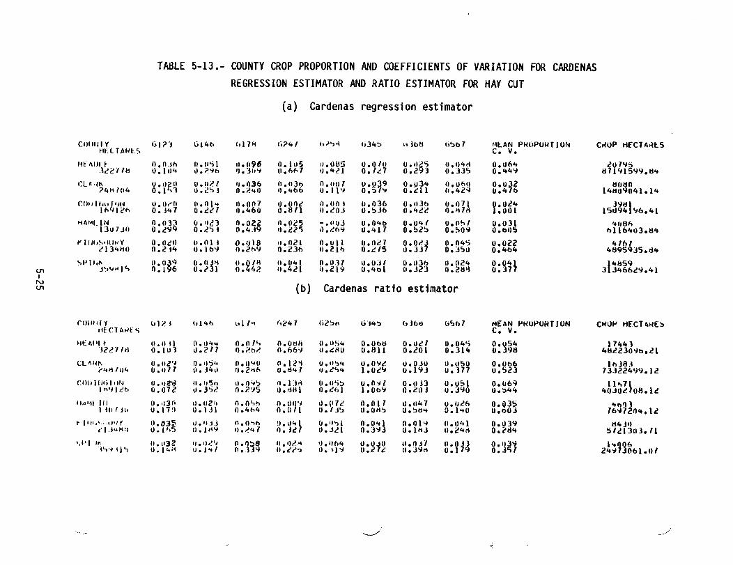
TABLE 5-13.- COUNTY CROP PROPORTION AND COEFFI CIENTS OF VARIATION FOR CARDENASREGRESSION ESTIMATOR AND RATIO ESTIMATOR FOR HAY CUT

(a) Cardenas regression estimator

CUI 1111 y 61n li14b "17~ Ij?41 1,""'" hJ4~ I.to/i ~,':>o7 '''I:.AN P~OPUlH ION C~OP ttfCTA~I:.S~IH TA~t:S c. v.

fil:: I\IJI ~ o • O.jt. 1I.1I'j1 tI.1I96 O. II'S I).GU5 0.0/11 U .11~5 1I.t)4ti 0.064 lO7~53alltl O.lu<+ V.?"jh fJ. ]lt~ O.M,7 I'.4,)I o. It!.7 0.2 j 0.335 0.44~ tH 141SYY. d4

CL t .~" 0.11211 0.111.1 11.036 0.1l)/) O.uIlI tI.u39 0.u34 Il.Ohll 0.0)2 MOdO?4H7U4 O. I" J U .l~':>j 0.1.<+0 'l.ltOO o.ll'J 0.57'1 O.ell 1I.42~ 0.476 14110'l041.14COlllh\> r /IN 11.11111 H.1l1•• 11.007 O.go" 0.110 t 11.036 O.ll]/) 1I.07~ Y·Ol4 3YIH

I"Q,,'''' o. j47 o .lll 0.460 O. fl II."OJ 0.536 O.4lc 0.117 .001 lSd941~b.41HA'~1.1 N o.tln (J.II;') O.OZZ 0.0"5 -.tllI) O.Olto o •OltI O.O~I u.031 4118f,1307JII O.lyQ O.~l)t (1.4J9 II.US Il.~h'J 0.417 0.52':> 0.509 0.005 fl11b4,)J.d4t< IIJI'~'HJh'Y O.OeO u.nl t 0.1118 11.021 O.Ull O.O~1 O.OI"~ 0.040; 0.022 4 If>"1134"0 °.2 t4 O.lo~ 1l.21>Y 1).236 u.Zlf) o.,US 0.33 0.350 0.464 4d95Q35.d4~PI'," o.o~q (J.()j/i U.O/Ii n.1l41 0.0.17 \J.O]I 0.1131> 11.024 0.04l 14~59

<.T1 J~J"".q 5 0.1 6 0.0:>31 0.442 11.421 iI.219 0.401 tI.J2J O.2d'i 0.31 3 J46629.41IN

(b) Cardenas ratio estimator<.T1

(" OUt if Y lJ 1i>. t h14" ~.1,••. (.247 C;2':>1I G'tlt~ btb/j b'i61 MEAN "'WPURT JON CWO•• ttfCT~~E~HEel A~f" c. v.

11£1\1'1 t: it.itiJ 0.114,+ o.ol~ O.OlHi (I.itSlt O.Otili o.ocl 0.04'i 0.354 17441J2~-' It! 11.111] tJ .?ll 1).?'tI'" O.b6ll 11.'::/'10 0.811 O.lOI 0.314 o. 98 4~1.2309b.ll

CL 1\I~" U.IIZ'I o. 'I'>" fl.U"''' o.12"t U .,l~lt 0.0':1'- u.O.Jo tl.lI~O O.Oob It>38.ti',+/i/u" II•uf7 ll.341) 1I.2>1fo I).d••, lJ.~c.,<+ 1.0c'J 0.19] o.J17 0.';)23 7J.l224Y9.12COli Hit; 1 ,)/~ u. iJZ'd ".1'')0 ".o'-l~ II. 1:H o.u'j~ 0.0~1 o.lIn O.o~1 0.06~ 11'>11Ih'lltb 0.072 u.h~ o.2~5 O.dHl O.~61 1.00'1 0.2,) j o.JYO 0.:>44 40JOl.loa.lc11,"11 III 1I.,)31i II. "Z!, O.O">!'! 11 • OWl 1).1I7t 0.011 o •it47 O.lItt.. 0.Q3!) ltlll)]ItufJII o. 17!) O.lJl 0.4#..4 O.ll/i I). I J~ u.Oti') O.':>n•• 0.1'+0 u.003 169720,+.12~ I'" I".'" "I ( n.035 ,'.'U.J 0.0"'''' ~I."ltl (}.11'l1 0.0'+1 0.01'1 0.1141 0.039 84 jtl

C 1.'41111 O. 1"5 nol~Y n ••.•••1 o. )21 U.Jl.l O.3'l.l 0.1113 1I.i:!lte1 O.t'd4 51113l1).11',PI '.,.. ".1132 1,.Il,!'J 0.°18 II.')I.-i '.1.tlo4 o·~r II.1IJ"1 II. Hi O.~39 1'+936t'-,"1 11 ') O.14H V.l •• ' (I •. J 9 lI."/o I)•.,1 'J (I. ~ 1I.39n O. 9 o. <\1 24~ Obl.OI

, I

'",-- "'-" ,J

TABLE 5-14.- COUNTY CROP PROPORTION AND COEFFICIENTS OF VARIATION FOR CARDENASREGRESSION ESTIMATOR AND RATIO EST IMATOR FOR ALFALFA

(a) Cardenas regression estimator

C()llN1Y 1.12J b14f> hl1" ht'47 C;?~H G14~ ldhti r,')b 7 "'f AN fJlWPOR T IOt~ CIJOP HEClA,U.SHfCTARI:S c. v.

M~ AIlLl: II.IIlf 0.0':1<:' /I.oni 0.1144 0.11.,•• O. OOll 0.Oh6 11.014 u.O'-9 ~~11}137171ti 11.11-\ 1I.~4t) II•21 ti I} • IIt'J 0.11i~ O.l':>l O.Ibl:l ll.29b 0.l31 I 51181').36ClAi(t' 0.11/,0 11.0111 0.114'<1 0.0." o. (,'" O.Ohl. O.Obl 0.034 0.v.5ti 14'i12

?4H7U4 0.11-,4 11.199 0.116 0.131 0.1 U 0.17~ u.l':i~ 1).1)] 0.l14 ~b5c;ObO.19COllii'll, ION U.Of>h lI.ul<; O.04'i I}.06 i 0.1113 II.Uh.J O.05~ 0.040 o.obl 111135

)6'1)1.6 1I.21? O.2~1 11.)('0 0.17~ 0.169 0.242 0.lti4 0.166 O.~OO 4l0l0b2.5~"A"lll\l 0.07'1 O.lItill 0.0"" 0.0"'" O.Oiil 11.0711 O.O'll O.C1~1 U.071 9278

1 JlIl311 u./flO o •21 '~ 1l.1,..H ,1.131> 0.11b o • 11:1•• 0.l14 o •I:J4 O.~O~ JbOti441.1lK)Ij(,,,d'hn O.lllh 1I.,lM•• 1I.1Ih'1 1I.06b (I.IIU 1I.01i~ 0.061 0.04'i 0.016 1!~H201.01~1]4~U O.?"''' O.lb2 O. 1 " ) lI.l?4 11.<"32 0.14'" 0.1':10 0.100 O.l3':i

<, ••• I~J" 11.1144 1l.1I'"i O.I}"" 0.04'+ Il.Ufl O.lInt U.?liI U.II"O 0.044 !·79')J':l'H ) ':> U • ) '15 O.~8'-i o • 441 O.ld-; II.~ 9 O.2Y4 O. 33 0.31~ 0.421 1+ ~24471.41

U1IN (b) Cardenas ratio estimatoren

rOIJ/<1 Y u I ;:>j (,1'+b Ii! I" 1;?47 \;2':1'1 63 ••':1 hJbb "'>67 MEAN Pt<OPO~TION CROP HECTA/'lt.SHt.l TAt<': <;, C. \I.

dFIIPlt 11.(1'51 O.ll/j /l.IlS] 1I.0~6 O.lItll 0.010 O.OJIi 0.041 0.051 ~83011t,?11 ~ II.I4 I) o. I f'l O.IJO 0.130 O.lhl O.)">b U.l00 0.106 O.~O~ 1 6a14~6.10

Cl :\·(t II.""'" 0.1164 n.1I5~ 1l.1l!;4 O.II';ih 0.002 U.03'" 0.047 0.U54 13':)13l'4H/1I4 11.1••3 0.140 0.13 O.U1 1).14':1 O. 145 u.llo 0.111 0.163 4~4 )44.21

(11111111,1·)N I) .115'. u.ah7 (1.11">" 1I.0~4 u.ut;•• o • 1}5~ 0.041 0.047 O.O')'t l1Uh4.l1In<'llt. O.litt$ O.)'J? /l.14" 1).1Jt.! 1I.1J~ 0.141 11.11" 0.11b 0.145"11,-1' J I~ 11.11611 II• 1I11 O./It'o o .u':::,4 0.059 0.u66 11.046 tl.OS7 O.ObO 1609

) -iU1]11 U. 16'~ II• Itd 1l.l/i tl.1J~ 11.137 0.14'" 0.1111 0.1H 0.1Jl 104HJ2.00~I~I.,..··.IJ"'Y ll.u61 0.0 II' 0.1152 0.!l'59 o •'167 O.OBI U.1/34 U.04h O.ObO 1274~~ I 'i4"11 11.144 u.IBA 1I.le'1l I) • 14 1 O.I'lO 0.181 0.090 n.l0n 0.to7 11 ')82421. lu"1-'11'1< 11.1160 (I.O/i 11.060 11.0'>" II.II A/. 0.010 1I.04t, O.O~l o.o~'" 21 J41i

-i.,'H 1':::J II.1511 H.ltli lI.141 O. 129 '1.14'" 0.)52 11.0.,,9 O.I1S O.lb'l 12961li66.tib

TABLE 5-15.- COUNTY CROP PROPORTION AND COEFFICIENTS OF VARIATION FOR CARDENASREGRESSION ESTIMATOR AND RATIO ESTIMATOR FOR GRASS

(a) Cardenas regression estimator

COUNJY li1 ,>3 6140 lilH r.;J41 h?~ti tJ14!> 113bii b5h7 ~It:/llll "~OPU~T ION C~llP tiECTA'~t::SHf( r At~ts c. v.

ItlAlJl1: O.u.,A 0.0,+1 11.044 0.0':>'1 II.U,'I O.IIIJb U.1I4~ U.llbM 0.0':') !11b4]2211ti o • 'J,+Ii d.l1b 11.1•..•7 u.t32 0.1 4 O.J!:J!> 0.2d O.t"lb 0.339 ) 910~t1".llCl 0\1o(~ 0.l1.4 o • wH (). ()~;4 1l.04H U.III.t> 0.0'/'1 lI.lIll 1I.03tl 0.o1l7 l~tl8q(,4li704 o.")••~ o. 00 (I.2?4 O.13lj 0.114 0.2)'1 Q.t!lIt 0.112 0.4A6 0':)25087.64CUIJ (1"'.TllN o. ~"7. ().11-).'1 o.n~~ 0.04t 0.U~4 O.o':>ti O.L1bJ O.O:lb 0.ub4 !08~n1""12b O. 1l<J o. HI 0.2(' o.lld 0.110 0.23';) O.)HJ 11.)24 0,"'J9 4 46 b31.9dHAIl! JN 1l.11~4 0.tl~4 0.0<,1' 0.0';)') 0."4" 0.117:1 0.07':> u. o~:>l 0.061:1 IiliJ4) )0 nil 0.261 o. HJ 0.2u7 0.)1i" 0.1:01 0.2'11i O.lh) o .If)2 0.2bb 6379492.1lt< I'·jh•../IU •.••Y u. lid II.I ~ 1 0.0" •• (1.)21 il.llli O.Dl o.OJ! -.0)3 0.Ofi6 ~d2171.1]4 fill O.2'N O.~ "> 0.h'4 (I.4)J t).:')]b 0.!))4 0.1 t.l 0.241 0.036 )3 258158.29SfJ 1"1( 0.0"<; 0.113'+ 1I.0?h U.ill1 0.1117 O.OYI O. 131. 1I.~08 g:n~ B094:i~I}>iI';) 0.J47 O.lbl O. 1 ,tH 0.221 0.t41 0.326 11.419 0.516 26 d 11 36. 12<.n

IN (b) Cardenas ratio estimator-....j

CIIu."TY u 1i! I 6140 Gl1ri lJ7.47 u2':i/i G34!:J GJbli 1;';)67 HE 0\1\1 PkOPOH fI ON CHUP HECTA~ESt11:('rA~tS C. v.HE"'II E 1I.11~2 lI.flfij 0.04'1 O.Ob! O.tl.,~ o.o~u 0.07~ 0.045 0.~68 ~1817

'377.'/IM 0.2f) 0.2b4 f1.1'><J /).lb 0.~00 0.211; 0.20 1I.1)~ o. 78 J 095179.70CLI\HI( tl./lnt. 0.07'; O.O4~ 0.052 0.044 o.OtiL O.ObJ 0.039 0.0°1 15072

£0'4 Ii111" 0.2HO 0.2bO o. I~~' O.lb'l O.IM,} 0.211 0.193 o • 130 0.30 C!051S003.71rOil1"'hlllN 11.0Hi. O.lI/t 11.044 0.il411 /l.04~ 0.1117 O·Ybg 8:~M g:~~~ 9!9;It. 120 0.c'H9 0.201 /).1'10 I) .161 0.11 O.~iJJ o. t:I 9S 7 63.tt4HA'11 IIII o.IIlA 0.11,1,1 t n.n'll 0.04R o .l141 O.OdH O.Ob~ 0.041 O.~~5 tlSFIJII73l1 0.3;'> 0.7U 0.20£' 0.142 iJ.l<;o o. 1~b 0.111 0.121 O. 6 ~19 Sti4.5uf(1"'h"'"lJ~Y 11.11-1" II.II~'') O.I}"''' 0.01" 0.1)1,4 0.103 II.OliO O.O~] 0.1)18 ~66S4? IJ4bll 1l.t!71 O.t1H 1).1'>'> '-1.20~ 0.1.13 o.23'J O.2"~ 11.)51 0.254 1 8444b4.5)

SP I ~l" ll.rJ4<J tJ.IIt:it> 0.0-;2 O.lJ'>~ 1I.IJ49 O.O~l o.yn 1l.04o.; O.Qt>9 5i~9B'J).84J'>""I!> ().2 ..i4 O.l.ol 11.11"2 C) • 166 0.119 0.211c'1 o. 90 o • 129 0.308

"---/

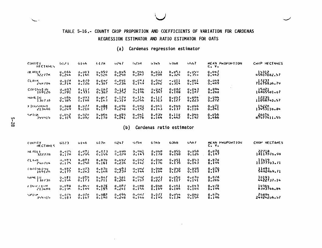
.••.•.... " '0 ~'

TABLE 5-16.- COUNTY CROP PROPORTION AND COEFFICIENTS OF VARIATION FOR CARDENAS

REGRESS ION ESTIMATOR AND RATIO ESTIMATOR FOR OATS

(a) Cardenas regression estimator

CIJl III H c, It') Glt.t. (·I/H ht'4 I c;c:!~ti Id ••~ hiot) 1).,"1 MEAN PI'<OPO~TION Ct<lIP HfCU~t::SI1fCTAkt~ C. V.dl-AIlI.F. 0.064 11.1'113 (1.059 0.U,+5 ll.lIh4 O.u:U o .1I'd ll.ll~'~ 0.047 1~3FJU f1H 0.244 O. 14tl 0.5~b 0.2'id 11.2(,7 U.~~H 0.324 l).o4~.• 0.,+42 451J() OOl.!JlCLAIIK O. ("Ii 11.011:) 0.011" tl.O~1 U.1I4J U.O~~ -.1I11 U.llnl O.Oh'l 17237t'4HI04 0.214 lI.at> O.)u"' '1.1.30 0.1..,<1 O.b:>~ v.J14 u.I<l4 0."k9 1 1)158j6.1~CliP Hll'~'IN IJ.IIR) O. H' 1l.!C12 O.I~H II.lOt. O.~'1~ u.O/:Jl ll.0404 0.094 .'j.i2~It. 120 0.1'91 0 •. "] o. ul ., • .?" l 1I.1M6 0 •. 4 o.lijij O.lHl 0.200 Ibd65 ttl.olliMIt 1"1 0.1184 U.Il'I) 1I.0h7 11.12~ tl.llh 11.117 o.o~' 0.Ufi4 0.~~4 12~35

!Juno I). "HI" o.I~H Il• ltd 0.:'1'" 1l.t.':>6 o.3D O.lia u.UJ O. 12 11058140.51I'J 1I1,';'HII4¥ O.Oijij 0.11" 0.080 U.O~O o .f) H(l 0.0,.,1 ().04li U.1I46 0.~71 ~5ljRc'1)4HCl 0.241.1 0.<:.'111 11.1"/1 0.240 o. 1'<;2 0.1 ••3 1).13' 0.116 O. 4 1 '+5 11b.a ••",.. I rI" lJ.U'">2 0.n211 0.064 0.05'; 11.0"1 O.O3~ 0.110 O.04b 0.05b 2°ffi

(J1 )':>~I1) ~ O. JI "i 0.1I9c' 0.170 0.241 0.1.16 U • J 04 0.442 0.191- 0.466 tiT!) 741l.5~IN00 (b) Cardenas ratio estimator

rOlp·,TY GI23 lJI ••6 lj(1~ 1;247 'J.~~1i 614~ GJots u'inl Mt:AN Pt<UPOIH IOl~ CROP l"Il::CUwEStlECT Akl:C; c. V.Ht.AI)It n. 'llL) 11.1171 n.OI.J (J.U.,JU 1I.IIH) O.C1tlti 0.05S O.O~O 0.u70 227~8

]Z7.nu 0.11H 0 ••.•0<, C1.I'>") O.??~ 11.14 t 0.110 o • 1':)0 O.llb 0.ln7 Id11 Olb.~HCLllriK II.1l7"\ 0.073 0.070 Il.U"'l 0.Oti2 O.Otltl 0.051 0.0':> ) 0.Ul0 17419?4t1 1114 o. I'''' (I•.!'">II 0.161 1l.~)4 II.J4~ tI.l'Ib 0.D5 U.14J 0.l'i14 1 311703./1( ll'lll"h~'IU /).01" II. ,,"/) 0.0711 n.~9 ) u.uMl U.Ol>b O,V'>~ 0.y';5 O'f9 ~1~9~It> I~h 0. 1 7 u •.!!)J C1.1h!) I). 3'J 1.1.144 o • Itilt O. ~ O. 5J O. \j 4~2 69.11'1""1. III 0.1111 11.070 fI.Otl' U.IOI 11.11'11 O.l/tiJ II.OSll C).C171) O.Old 1019]

I HI 1311 1l.I'Ih o.Jlj O.?ll O.lb'+ O.b" O.t!U O.l1l 11.1"'1 O.lOb 4422131.14r. 11'1')',' lHl' 1I.1I7U II. 06'~ n .0 7S 0. OA, O.vl:lO O.Obti O.lIhJ 0.04l 0.0'0 14964

t'D ••tI/) II.1..,,., (I.IH'l /).151 n.~41 lj. 1''In O. 1b'J o .1l:S4 0.1()~ O. I~4 tU"I3144. tt4',PIII~ ll.II14 o. Ill" (I.UB? (1.096 O.lltll o.on 0.11')4 O.Otoll O.Cll'> 2~!J94.t"~111~) 0.18t O.ltl"' n. PHI C1.t!40 l).14o o • I~'j o • 1 J4 (1.1'.>h 0.J~6 24~242116.!)1

TABLE 5-17.- COUNTY CROP PROPORTION AND COEFFICIENTS OF VARIATION FOR CARDENASREGRESS ION ESTIMATOR AND RATIO ESTIMATOR FOR WHEAT

(a) Cardenas regression estimator

COllNTY r.1lot (Jj1tb b17d h?4 I h'>~H G34., l>3bti l''''t> 1 ME AN t>IWtlOkT 1011I CHOP tiECTARI:ShfCTAW~S C. \/.

HI:AllU U.O<;h 1l.IIYii H.n .•11 1I.1141 ".lI4 j u.u.,l 0.03u u.u/,,) 0.tl"t5 I1bIJIl??71U 0 •.316 O./SO 0.117 n.324 1I.1j'l O.JhJ u.22.i o.~o., O.J~A 4'14'12?'>'I.'j~

r.L AI~l\ 0.061 O.I'>.i 11.1"0 o. j4~ (I. 1"t1 0.1l1 O.Hd 11'19'" 0.14'1 3b'l51(:I4H/H4 0.0,,13 0.1"3 o • I'11 11.15'1 II• 1">2- 0.14 •• 0.21'+ iJ. 10 0.1.33 131101~';)1I.114COlli M. r flN U'I 'h 1I.lb, o·f/o ".1bt (I·tM 0.1-'1 0.u27 u.lEU O·14~ 231)0~

lh912b O • .i3 0.1'13 n. 01:> o. ~li H. r.ll o.lt>o o.l~d 1I• 19" O. t. 1372IBJ7.5~HAMLI~ 0.tl1 O.:rH , 1l.?lIl 0.174 O. 1h2 u.l~7 o.lAo 1I.t!./~ O.2~9 2130l1]111]0 o.l41 0.2JI O.lflfl O. 1';)1- 0.14<;) 0.114 0.1 4 11.201 0.1 2 2216tt6 ••3.o4K 1~/('~I-iIUJY lI'I"lk (1.11'+ 1I.po o '16" 0.1.13 0'140 ll.lS3 11.2/9 O·rn 41HO21]411(1 O. b. O. Pi! O. -:'0 O. 49 O.lIO O. 2~ 0.271 0.228 o. b1 1154 .4a!;.4j<'1-'INt- O.lI~H O.OYO 0.~()4 0.067 ll.li'l7 0.lI7t 0.058 0.0'11 0.075 26'tF

U'I)~<i.q~ 0.162 0,.'\I)t> 0.11 0.22/1 0.301 0.213 0.171 0.2'10 0.242 42-:'';901.93

IN

(b) Cardenas ratio estimator1.0

CIJlltl1Y lJ12j h14b G11'i r,~lt7 (jl.!>~ C;14~ bJod (;501 ~I::AN PIo(OPORT10N CROP H£CTAIJI:S/-It C TAI<~5 C. V.

HE: 11.,\ t 0.116'"' II.II h 0·1'1 o·tOI 0.1I9<i 0.O9~ O.O~2 ().~46 0.106 J~~~~~"1 •.,S]i!?nri 11.11'19 !J.ll1 O • .l o. 21 1l.IJIi '1.I':> 11.131 U. Od O.ldOr.L(\11K lI.nay U.I\'i n.11I6 O.tl~"" 0.094 0.lu3 O.U~U o.12ii 0·1°3 2Srn

£, •• /1104 ll.114 1).1.0 O. 135 O.l1'J /J.IJb 0.211 O.IJ] 0.117 O.JS 120 Y9llt.U

1'/1111 j .•• ; T fiN 0.1191 o.!?) 11.105 n.09] U.1I42 IJ.}lIb 0.091 0.121 O·to~ !7l~'Ih'll£'f:o 0.111 0.14 j 0.1~4 0.110 0.13d O. 2b 0.134 0.16] O. t. I)~' 2bll.2'111"~!L 1/·/ lI.h~4 1l.1~1 /I.,Z~ ,,·tf)J 1I.IOb 0.11"11 11.1'~ 0.132 0.1+4 llt<JH1]117 Hl 0.' ?4 II.II") 0.1" O. tJ 0.1 hO 0.114 II. 54 ° . 1So O. I 1 b'l~N3J.4Jto 1'1,,',1 II~'~ /I.07H II.I'U /1.117 II. pI. O.llth O.IIH'+ O.04J /l.~7~ o.IO'il 2n3~I' V.,III U.()~/1 o. I~o O. J'> O. 47 1I.14/i 0.11~ 0.1 <;0 II. 5 (I. ~ba Jlj9j St4.lib

'.P I' I~ " .1I6A II.'jS 0'119 O·llh n'l°<' O.U'JU O·tflh H:ta~ 8:1~~ 4111HH.l'~'I"I"l n. I01:> 11.14 I o. 4"l II. ~.J .1. 4'..1 0.1116 II••• 3 5J3t>07u!J.14

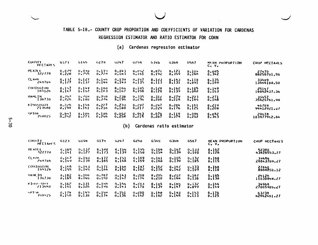
! I\--- \"../

TABLE 5-18.- COUNTY CROP PROPORTION AND COEFFICIENTS OF VARIATION FOR CARDENASREGRESS ION ESTIMATOR AND RATIO ESTIMATOR FOR CORN

(a) Cardenas regression estimator

CUI,p·HY uln C,146 (0) 7H \;1.47 Ij(,'':)'i (, .1It';) 6JbH (;<)h7 Mt::l\N"'t<ClPUPfION C~I)j.J HI=:CTA~t-_SH~ C T MH: ~ c. v.

l~lAm~_ II.O/Y II.n'IU U. II 'l o •I) 4 J O.H':>t 0.071 0.12. 0.}01t O.OIi'> 27470.luna o.u~ 11.1.'>5 o.??~ 1I.1"} I).ltil II. 1'Ie:. O.J~~ 0.268 0.342 882567t)1.5~CLA •.•." O. \11 O.lt, 0.1 ••t) o.p~ H.J.,7 o.l~J 0.143 11.110 0.135 J3~091.4'i7UIt 0.11.7 0.131 11.144 O. 4'~ 11.13<; 0.113 o. 31 0.0':11 0.10~ 13444108.50COil (MH ml o. )',7 O. 14'l O·lbtl O.JI)•• o.I1i5 O.lt'tt 0.142 0.125 O·14~ ~s!4 1JhCJlb> 0.147 o. Il)~ o. ,...) 0.11)1 0.1 S8 0.120 0.13~ 0.0 d o. b3 Ibtt 2431.30HAMLIN 0.1.'1" C1.-'UH O. ~'JO o. po 0.31'5 0.311- 0.27'1 0.22) O.21A hltS7J3C17JII II.;':»8> O.JdU O.2~" n. 9n o.t]/) O.2tsb 0.21H O. 1bo; 0.1" JSb2S1b1.'ldK ["lh~HlJ,?Y o.f'r'f) O.I':lti 0.2?7 0.233 0.t!'l1 0.2'+7 0.204 0'161 O.21<J 4blb9?lJ4tiO 1.1.IYO O.lbJ 0.2Jb O.ldd 0.2J 1 O.2t!<J 0.17b O. 20; 0.20d 94412n1.u/<;P1N" 0.0" 'J o.ll\H O.ll1h o.~':it! 0.043 0.07j 0.1~'l 0.~94 0.1I~2 29fl714.l'>'lHJ'j 0.2'>2 0.211 0.7.4h O. Sii 0.215 0.2ti 0.3 ~ O. S2 0.343 10H719n2.84

<J1Iw (b) Cardenas ratio estimatora

COI 'tITY (;12.3 lJ14b HJ7'i l.t41 G2';)d G14~ (;3 bf:t Gljb7 MEAN PIWPUPT ION CtWP HECTA~tSHF.CIAwts C. v.In MIl t I)• 16') 11.131 1I.lrHI I) • 1')1) o • 1'15 o '164 0.167 O. 1J.J 0'162 S2~8g·427.71tl v.l"l 0.1t?1 0.1/3 o .13~ II• IStt u. S4 O. 3~ 0.100 o. 26 434 6 ';3.27c: lllt~ I< c) • it·, 7 0.1411 n.1 n lI.l~l lI.lfi9 II• It>>! 0.165 O.13l 0.160 3~"1J"t'1t~7114 11.14"1 (I. 1 ]Q O. 165 0.148 I) .159 0.lb8 0.130,/ 0.10~ u.11S 2084316'1.i!7{"()tlli'lC;rClN o. Ih>4 11.14] O'Pl n·14H U'11i7 O'lbt O·tM O'p~ 0.160 21042113'1120 O. 1'i5 o .14') II. t-. O. ~2 O. 62 O. -/tt o. 4l O. 0 o. 10 8tJl:4850.12.HA•••t I tl 0.102 11'1hll (1.;»07 U'143 O.too 1I.20~ 0.212 0'161 0'18S 2412AI.J07JII 0.169 O. 4!) O.lli(1 o. '+7 0.1"14 o.t!ltt 0.16 •• o. :.to O. 3d 110JOf}4d.UI< II·jo.···~llIJ'f /I. 16? u.1JI O.I'~li l).lh4 O.CllJ 0.105 ll.1t1~ 1I.13l 0'164 349M1.1)4Mll U.141 o.lll:> 0.1"';) 0.1"3 0.170 0.130; 0.147 a.OIN O. 4'i 1106SQO!).c(/".." ;"' i). 174 O. ) 4'1 Cl.l'//'1 a.1Sl II.~OO O.lt1tt o .1'~J 0.1 ':).'} O.p6 63c?3'3t'>lJ'iI':l (J.I'>O 0.1311 11.174 ll.136 Cl.162 O.lttl o. 48 0.113 o. 25 o2!i42461.21

TABLE 5-19.- COUNTY CROP PROPORTION AND COEFFI CIENTS OF VARIATION FOR CARDENASREGRESS ION ESTIMATOR AND RATIO ESTIMATOR FOR SUNFLOWERS

(a) Cardenas regression estimator

r.(HI·~T y Ij, ;>j G140 GI7H 117.47 r,2"H ';J4~ u)t>ti h~ol ~l£jlN "'1<t()POIHIUN Ciolfi!>Hf.CTA~t:.SliE C r AJ-f s C. 1/.

Il~. API. E 0.04~ II.U~O 1I.0t>O O.Mh u.O"tl:l ().o••2 O.(IC7 1I.0~d O.Il~l 1b41~JU 71M o.t!o (). ,u'> 1).7.42 11.1:112 u.t.n' lJ.7.o~ 0.234 O.JOO 0 •.J4~ ]2142077 .07CLI\I"'" U.U·i4 11.0••4 0.036 n.oSa 0.1148 0.05b Cl.023 0.03h 0.046 !I J9574~7u4 n. '•..•4 o.~I!) 0.)1')] 0.S!:>4 0.334 0.2!l1 0.136 0.lb7 0.434 2 4423~9.27Cll'llrll' TI)I~ 0.1l4B 0.1147 11.041') n.o~., 0.1143 O.OSli 0.021 0.044 0.1148 816510"'126 0.1 tiC} 0.233 (I.I~? 1).614 11.~14 0.21!> 0.10'1 0.19<; 0.430 III 5~1~.70tlMlll~1 U.1I51 O.Ot'l1 o.olin n. I!l~ 0.1150 O.ut'lo 0.023 0.~74 0.072 9403)JII7311 0.2(13 0.241 II•?.J1 0.ti19 0.2~? 0.24M 0.O9~ O. !>1 O.~45 26U6110.55K I'-JI,c;tIIII-iYII.U"<; 0.04'1 0.011 O.0!:>4 O.II7.d 0.01.1 0.OJ3 0.Ob4 1I.04K )0~4421341111 0.l43 O.4~1 u.3<+6 0.444 0.237 O.)lJ!> 1.1.270 0.41lJ 0.351 Ilb 351tt.d6..,p I~J" \J.0311 0.u21 -.Oll 0.0')0 0.lIfl5 0.04~ 0.112') O.O}J O. 030 )0~25

Ul)0:;'-1-11" D.hl) 0.401i O.I?') 0.165 ).ll~O O.oJII O.lti~ 0.4)lJ 0.A04 7'i151934.'0

Iw

(b)•.....• Cardenas ratio estimator

(011'/1y ti123 u141:1 G)7d (;241 b2~'" u)45 b311K 6~6·' HEliN PROPOIH ION ClotOPHECTARE,)tIt:( TAPt:.s c. V.Hflllll.f u.O:l~ O.IIZ'I O.OH 0.0"') 0.(1)0 0.040 I).Ol7 0.026 0.034 &091332? 1/11 \J.29 0.2!>4 11.0 0.344 o.~54 0.3~7 0.200 0.209 0.398 1 n99 18 •••1CL '''''K II.0J4 O.lll'> n.n}" n.o~':i 0.0413 0.03~ O.O~l O.02A O.03~ 816814A/04 0.]02 O.~)o /).0 Ii 0.394 0.49) 0.304 0.1 l 0.235 0.42 1210538J.1J4r.UlllM;Tilr-l O.O~h O.Ot!] 1I.0j? 0.051 0.048 0.037 0.02~ 0.O2~ O. t)~3 6~31~j2.)210'112"" 0.")96 O. I"'., lJ.Ot1\) 0.424 0.4"0 0.27b 0.15 0.250 0.4 2riAMl.)N 0.050 O.IIt!!> n.o)':; n.07~ 0.0"0 0.03'1 0,Y2A 0.03R 0.041 ~JS6I H) 7JlJ 0.4nfl 0.1':i4 0.Ott5 0.486 0."0'1 0.22~ O. 2 o.21i!:) 0.5l0 1 61323.96I<: IrJr,s,,"·~y ".n~5> o.Ojl') 0.013 0.041 O.OSI O.OS!> 0.O3~ 0.024 0.O3~ 7444

II j4~11 0.20) 0.1)~ (1.0112 0.28l 0.071 0.444 0.1.4 0.162 0.41 9511024.10'.1-'lilt< 0.040 ().1)211 n.o~4 11.01:15 (I.1IC,6 o.o .•!l 0.025 0.033 0.~3g !f901')4'\15 0.317 0 •.:'07 11.0 '# 0.407 0.'+77 0.l~2 0.105 0.l41 O. 3 3 1l9tt07.8••

each county. For example, in Beadle County the proportion estimate of range-land using the training group G123 is .366 of the total hectares in the threestrata over which the estimate was obtained. The corresponding "coefficientof variation" is .356 and is defined as the ratio of the square root of thevariance, calculated by the formula, and the average of the hectarageestimates across the eight training groups. The next to the last columncontains, for each county, the mean proportion estimate of rangeland and thesample coefficient of variation. In the last column are the estimatesrepresented as hectares.

By comparing the "coefficients of variation" that were computed using theformula variance for a training group to the sample coefficient of variation,

..•one can see that the variance formula of Y, which was derived under theassumption that the within-county variance is equal for all counties, seems tounderestimate the true variance.

"") 5.2.2 BEHRENS-FISHER TESTIn tables 5-20 and 5-21, the same two sample tests used to evaluate the biasof the current county regression estimator was used to test for bias in thetwo Cardenas estimators. The corresponding confidence intervals for theestimated biases are in tables 5-22 and 5-23. The same caution encouraged inexamining the results in the first application of the test is advised herealso. Because the hypothesis for the Cardenas ratio estimator is rejected for10 crop-county combinations and the hypothesis for the Cardenas regressionestimator is rejected for 8 combinations, both estimators can probably beconsidered biased by this test.

5.2.3 F-TESTS OF VARIANCEThe two-sided F-test was used to provide some idea of how the variance of thecurrent county-level estimator compared to the variances of the two Cardenasestimators and how the variances of the Cardenas estimators compared to eachother. These tests cannot be appealed to unequivocally because one of the

~ assumptions for performing the test is that the samples are from independent

5-32

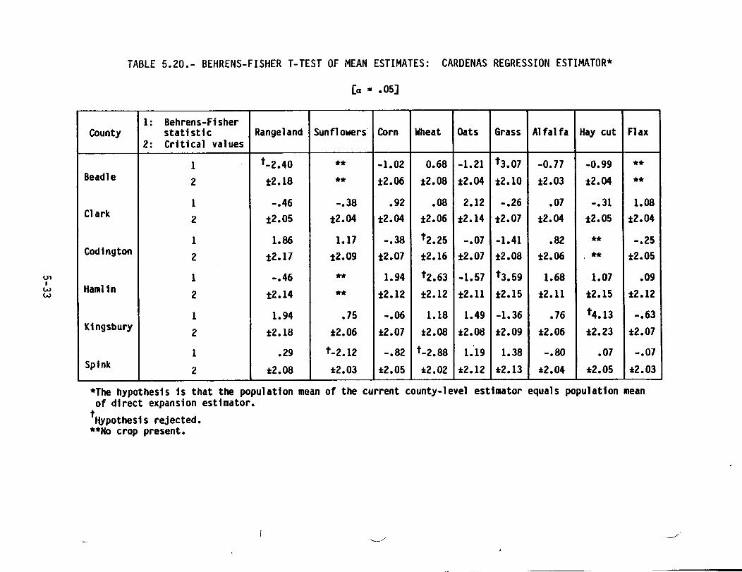
UlI

WW

TABLE 5.20.- BEHRENS-FISHER T-TEST OF MEAN ESTIMATES: CARDENAS REGRESSION ESTIMATOR*

(0 • .05]

1: Behrens-FisherCounty statistic Rangeland Sunflowers Corn Wheat Oats Grass Alfalfa Hay cut Flax

2: Critical values1 t-2.40 ** -1.02 0.68 -1.21 t3.07 -0.77 -0.99 **

Beadle 2 t2.18 ** t2.06 t2.08 t2.04 t2.10 t2.03 t2.04 **1 -.46 -.38 .92 .08 2.12 -.26 .07 -.31 1.08

Clark 2 1;2.05 t2.04 t2.04 t2.06 t2.14 t2.07 t2.04 t2.05 t2.041 1.86 1.17 -.38 t2.25 -.07 -1.41 .82 ** -.25

Cod1ngton 2 t2.17 t2.09 t2.07 t2.16 t2.07 t2.08 t2.06 ** t2.051 -.46 ** 1.94 t2.63 -1.57 t3.59 1.68 1.07 .09

Hamlin 2 t2.14 ** t2.12 t2.12 t2.ll t2.15 t2.ll t2.15 t2.121 1.94 .75 -.06 1.18 1.49 -1.36 .76 t4.13 -.63

Kingsbury 2 t2.18 t2.06 i2.07 t2.08 t2.08 t2.09 t2.06 i2.23 i2.071 .29 t-2.12 -.82 t-2.88 1.19 1.38 -.80 .07 -.07

Spink 2 t2.08 -J:2.03 -J:2.05 -J:2.02t2.12 t2.13 -J:2.04 -J:2.05 -J:2.03*The hypothesis is that the population mean of the current county-level

of direct expansion estimator.t~pothesis rejected.**No crop present.

estimator equals population mean

U'1I

W.$:>0

1 i. {

~

TAI3LE 5-21.- BEHRENS-FISHEl< T-TEST OF MEAN ESTIMATES: CARDENAS RATIO ESTIMATOR*

[a • .05]

1 : Behrens-FisherCounty statistic Range land Sunflowers Corn Wheat Oats Grass Alfalfa Hay cut Flax2: Critical values1 t-2.96 ** 1.53 t3.59 -0.40 t4.13 -0.86 -1.27 **Beadle 2 t2.04 ** t2.04 t2.06 t2.03 t2.10 t2.03 t2.03 **1 -.58 -0.76 1.62 -1.21 t2.55 -.47 -.12 1.17 1.76Clark 2 ±2.06 t2.03 t2.04 t2.03 t2.05 t2.04 t2.04 t2.12 t2 .041 2.02 .39 -.08 1.24 -.81 -1.60 .53 ** -.51Cod1ngton 2 ±2.08 ±2.08 ±2.06 t2.06 ±2.06 ±2.06 ±2.06 ** t2.051 .22 ** .52 .41 -1.86· t3.28 1.21 1.29 -.60Hamlin 2 t2.ll ** t2.ll t2.ll t2.10 t2.17 t2.10 t2.16 t2.ll1 1.91 .18 -1.11 -.50 1.45 -1.62 .10 t7.4 -1.18Kingsbury 2 t2.06 t2.06 t2.05 t2.06 t2.06 t2.05 t2.06 t2.24 t2.051 .42 -1.92 t2.21 -1.99 t2.65 2.08 -.16 -.07 t3.41Spink 2 t2.0S t2.02 t2.03 t2.02 t2.05 t2.05 t2.02 t2.04 t2.05

*The hypothesis is that the population mean of the current county-level estimator equals population meanof direct expansion estimator.t~pothes1s rejected.**No crop present.

U1IWU1

TABLE 5-22.- CONFIDENCE INTERVAL FOR ESTIMATED BIAS: CARDENAS REGRESSION ESTIMATOR[95% confidence]

County Rangeland Sunflowers Corn Whea t Oats Grass Alfalfa Hay cut Flax-13.106 -2.034 0.792 -2.196 2.634 -1.335 -2.488Beadle ±1l.887 ±4. 106 ±2.430 ±3.701 ±l. 796 ±3.576 ±5.147

-1.897 -0.842 2.037 .184 2.814 -.571 .098 -.412 0.913Clark ±8.432 ±4.54l ±4.530 ±4.971 ±2.840 ±4.524 ±2.834 ±2. 710 ±I.7329.638 1.476 -.927 4.485 -.185 -4.327 1.234 -.754COdington ±1l.212 ±2.651 ±5.085 ±4.300 ±4.401 ±6.353 ±3.116 ±6.097

-2.552 7.410 7.045 -5.699 3.430 2.463 1.072 .191Hamlin ill. 911 ±8.078 ±5.680 ±7 .627 ±2.058 ±3.l07 t2.152 t4.541

10.238 1.071 -.203 3.856 1.805 -4.367 1.174 1.256 -.957Kingsbury ±1l.502 t2.956 ±7.272 ±6.780 t2.516 t6.716 t3.183 ±6.793 ±3.144.969 -4.939 -1.663 -7.761 1.269 2.373 -1.234 .076 -.045Spink ±6.992 t4.739 ±4.144 ±5.448 ±2.265 ±3.679 ±3.16l t2.277 ±1.281

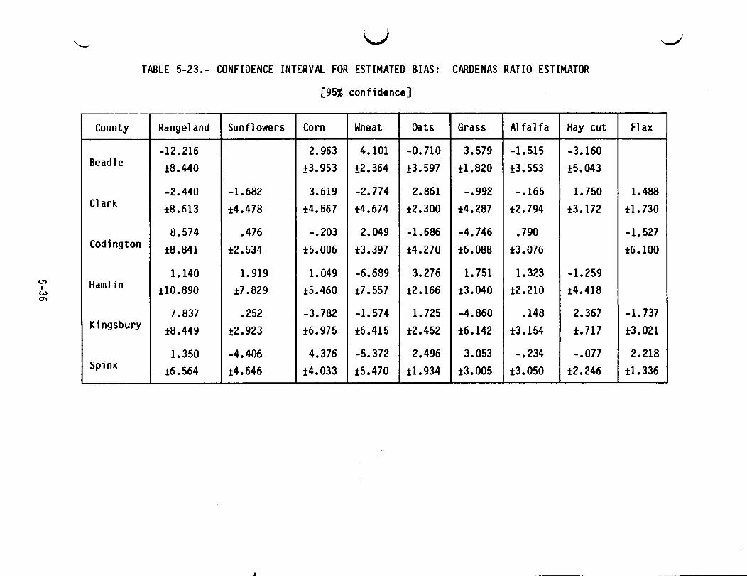
,-. uTABLE 5-23.- CONFIDENCE INTERVAL FOR ESTIMATED BIAS: CARDENAS RATIO ESTIMATOR

[95% confidence]

U1IW0'\

County Rangeland Sunflowers Corn Wheat Oats Grass Alfalfa Hay cut Flax-12.216 2.963 4.101 -0.710 3.579 -1.515 -3.160Beadle t8.440 ±3.953 ±2.364 ±3.597 ±1.820 ±3.553 ±5.043

-2.440 -1.682 3.619 -2.774 2.861 -.992 -.165 1.750 1.488Clark t8.613 t4.478 t4.567 t4.674 t2.300 t4.287 t2.794 t3.172 t1.730

8.574 .476 -.203 2.049 -1.686 -4.746 .790 -1.527Codington t8.841 t2.534 t5.006 t3.397 t4.270 t6.088 t3.076 t6.100

1.140 1.919 1.049 -6.689 3.276 1.751 1.323 -1.259Hamlin t10.890 t7.829 t5.460 t7.557 t2.166 t3.040 t2.210 t4.418

7.837 .252 -3.782 -1.574 1.725 -4.860 .148 2.367 -1.737Kingsbury t8.449 t2.923 t6.975 t6.415 t2.452 t6.142 t3.154 t.717 t3.021

1.350 -4.406 4.376 -5.372 2.496 3.053 -.234 -.077 2.218Spink t6.564 ±4.646 ±4.033 ±5.470 tI.934 t3.005 ±3.050 ±2.246 t1.336

populations. The overlapping training groups obviate· satisfying theindependence criterion; however, keeping in mind this limitation, the resultsin table 5-24 indicate that whenever there is a significant difference invariances, the Cardenas regression estimator and the Cardenas ratio estimatorappear to have larger variances than the current regression estimator.Additionally, there seems to be no significant difference in variances of theCardenas regression and the Cardenas ratio estimators.

5.2.4 RESULTS OF THE CLASSY-BASED DIRECT PROPORTION ESTIMATION PROCEDUREThe CLASSY-based direct proportion estimation procedure using the maximumlikelihood approach or the least squares approach can be outlined as follows:1. Apply the CLASSY clustering algorithm (noncrop specific to the county of

interest, sampled 1/64) to estimate m, p(xli), and ai.2. Randomly choose 500 labeled pixels from the segments within the county of

interest.3. Use the maximum likelihood approach described in section 2.3.1 to estimate )

ati•4. Use least squares approach described in section 2.3.2 to estimate ati.

m5. Compute the proportion of class t as wt = ~1 ai ati

6. Repeat steps 2, 3, 4, and 5, 50 times to estimate the bias and MSE of wt•

The procedure was also carried out without using the maximum likelihoodapproach or the least squares approach; the 500 labeled pixels were used tocompute the proportion wt directly. This is referred to as the simple randomsample approach. The number of labeled pixels in each county are as follows:Beadle, 8442; Clark, 7264; COdington, 5430; Hamlin, 3588; Kingsbury, 6086; andSpink, 9480.

5-37

<..nI

Wco

\..JTABLE 5-24.- F-TESTS OF VARIANCE

[Critical values: FO•01;7.7 = 0.143. FO•99;7.7 = 6.99]

County J1ypothesis* Rangeland Sunflowers Corn Wheat Oats Grass Alfalfa Hay cut FlaxHI t8.37 t31.16 t20.97 0.38 1.77 0.57 0.25 2.37 1.35

Beadle H2 .75 t18.18 t10.32 .29 .70 .62 .18 1.31 1.01H3 tU.12 1.71 2.03 1.30 2.53 .91 1.43 1.81 1.34HI 2.75 t7•67 2.70 t13.41 4.45 1.42 .47 .91 t.U

Clark HZ 4.36 3.80 4.18 2.18 .71 .44 .24 4.48 t.12H3 .63 2.02 .65 6.15 6.25 3.20 1.99 .20 1.03

HI tH.65 tI8.83 3.31 tI3.67 .53 1.61 .60 2.90 t.08Codlngton H2 1.85 t9•61 1.75 .87 .17 .36 .25 t7.36 t.09

H3 6.31 1.96 1.89 t15•71 3.07 4.45 2.43 .39 .81HI t9.47 tI79.90 4.75 6.98 .38 .80 .51 2.70 .87

Hamlin H2 1.84 t53.14 1.47 2.20 .15 1.16 .15 3.39 .29H3 5.14 3.39 3.23 3.17 2.50 .69 3.46 .79 2.97HI t21.38 t21.74 6.85 t7.38 1.33 t7.94 .73 1.85 .24

Kingsbury H2 2.08 t16.42 1.96 2.49 .83 1.05 .59 2.17 t.09H3 tlO•27 1.32 3.49 2.97 1.60 t7•58 1.25 .86 2.83

HI 2.50 1.16 6.02 .37 1.37 t7.36 .16 .51 .26Spink H2 1.25 .56 3.64 .46 .39 1.65 t.05 .41 .53

H3 2.00 2.09 1.65 .80 3.51 4.46 3.41 1.26 .49*Hl: Variance Cardenas regression estimator equals variance current regression estimator.

H2: Variance Cardenas ratio estimator equals variance current regression estimator.H3: Variance Cardenas regression estimator equals variance Cardenas ratio estimator.

tJ1ypothesls rejected.

5.2.5 STATISTICS FOR DIRECT PROPORTION ESTIMATORSIn tables 5-25 and 5-26 are some statistics that were calculated for each ofthe direct proportion estimators. For each crop, the bias, mean squarederror, and F-ratio are listed. The bias is the difference between the averageof the 50 proportion estimates of a crop given by the particular estimator andthe proportion of ground truth of that crop in the sample segments that are inthe county.

The mean squared error (MSE) is the average of the squared errors over the 50runs. The F-ratio is the ratio of the variance of the 50 estimates given bythe direct proportion estimator to the variance of the 50 estimates obtained,each using a simple random sample of 500 labeled pixels to compute theproportion directly.

There seem to be no significant differences in variances of the CLASSY direct-proportion estimators using the simple random sample approach and either themaximum likelihood or the least squares approach.

5.2.6 RELATIVE BIASES OF ALTERNATIVE COUNTY ESTIMATORSTable 5-27 lists the relative biases of each of the alternative county-levelestimators considered. The relative bias is defined by the equation:Relative bias = estimator proportion of cro~ - true proportion of croptrue proportl0n of crop

The true proportion of a crop in a county is declared to be the proportion ofthat crop determined by all of the ground-truth pixels in the sample ofsegments from that county. It can be seen that the Cardenas estimatorsproduce relative biases consistently larger than those of the direct propor-tion estimators, which appear to have about a lO-percent relative bias.

5.3 STUDY RESULTS: PREPROCESSINGThe preprocessing study was to determine if any of three candidate preproces-sors might improve crop area estimation at a county level by correcting for

5-39

UlI.~o

I "

~

TABLE 5-25.- BIAS, MEAN SQUARED ERROR, AND F-RATIOUSING THE MAXIMUM LIKELIHOOD APPROACH

[Critical values: FO•01;49,49 ~ 0.511, FO•99;49,49 = 1.97]

Grass Alfalfa Hay Cut Flax OtherCounty Mean Mean Mean Mean Mean

KidS squared F-ratio Bias squa red F-ratio Bias squared F-ratto Bias squared F-rat to Bias squared F-ratt0error error error error error

Beddl e -0.0003 0.0000 1.15 0.0119 0.0003 1.20 0.0010 0.0001 1.10 No crop present 0.0137 0.0042 1.29CIark -.0023 .0001 .96 -.0013 .0001 .95 -.0001 .0001 .82 -0.0016 0.0000 1.06 .0039 .0004 1.35Codi'lgton -.0036 .0002 .88 .0067 .0001 1.08 No crop present .0008 .0001 1.09 .0125 .0006 1.12Hall,1in -.0056 .00ill *2.43 .0480 .0021 *7.67 .0216 .0006 *8.12 -.0049 .0003 *3.91 -.0066 .0013 *3.75Kingsbury .0108 .0003 .89 -.0062 .0001 .70 -.0010 .0000 1.55 -.0031 .0001 .98 .0108 .0003 1.08Spink -.0024 .0000 .82 .0006 .0001 1.04 -.0013 .0001 .92 .0017 .0000 1.18 .0041 .0003 .60

Range Iand Corn Wheat Oats SunflowerBeadle -0.0400 0.0018 0.75 0.0123 0.0003 0.69 -0.0006 0.0001 1.06 0.0020 0.0001 0.97 No crop presentClark -.0035 .0004 .95 .0139 .0003 .83 -.0130 .0003 .69 -.0017 .0000 .86 0.0058 0.0002 1.31Codington -.0079 .0002 .98 -.0256 .0008 .66 .0070 .0002 1.15 .0109 .0003 .96 -.0009 .0000 1.12Haml in -.1439 .0207 * .31 .0701 .0061 *5.44 -.0328 .0013 1.93 .0542 .0040 *7.21 No crop presentKingsbury .0074 .0003 1.03 -.0200 .0005 .54 .0052 .0002 .91 -.0003 .0001 1.09 -.0036 .0001 .99Spink -.0097 .0004 .90 .0073 .0002 .68 .0021 .0002 .83 .0004 .0001 1.05 -.0027 .0001 .55*Hypothesis rejected.

(J1I

+=-•....

TABLE 5-26.- BIAS. MEAN SQUARED ERROR. AND F-RATIOUSING THE LEAST SQUARES APPROACH

[Critical values: fO.01;49.49 = 0.511. fO.99;49.49 = 1.97]

Grass Alfalfa Hay Cut Flax OtherCounty Medn Mean Mean Mean Mean

Bus squared F-ratio Bias squared F-ratio Bias squared F-ratio Bias sQua red F-ratio Bias squared f-ratiot!rrur error error error error

i\eddll~ -0.0007 0.0000 0.92 0.0084 0.0002 1.23 -0.0007 0.0001 1.07 No crop present 0.0150 0.0004 1.24::1 ark -.0044 .0001 .95 -.0015 .0001 1.05 -.0034 .0000 .76 -0.0031 0.0000 1.04 .0079 .0004 1.38Codington -.0021 .0001 1.01 .0060 .0000 1.09 No crop present .0035 .0001 1.19 .0145 .0006 1.08Haml in -.0161 .0003 *2.08 .0388 .0019 *7.11 .0051 .0002 *6.81 -.0223 .0011 *7.1B -.0722 .0071 *5.68Kingsbury .001a .0001 .92 -.0084 .0001 .71 .0002 .0000 .99 -.0011 .0001 1.02 .0225 .0007 1.14Spink -.0037 .0000 .73 .0010 .0001 1.43 -.0029 .0000 .90 .0014 .0000 1.14 .0040 .0003 1.00

Rangeland Corn Wheat Oats SunflowerBeadle -0.0418 0.0019 f).66 f).0183 0.0004 0.68 0.0000 0.0000 1.03 0.0015 0.0001 0.94 No crop presentCIark -.0086 .0004 1.02 .0159 .0004 1.08 -.0101 .0002 .61 -.0015 .0000 .79 0.0092 0.0002 1.52Codington -.0074 .0002 1.03 -.0370 •0014 .56 .0102 .0002 1.28 .0142 .0004 1.16 -.0019 .0000 1.03Haml in -.1729 .0306 *2.96 .1541 .0262 *10.48 -.0181 .0010 *5.09 .1030 .0122 *10.36 No crop present'<ingsbury -.0063 .0002 .85 -.0191 .0005 .65 .0152 .0003 .96 .0002 .0001 1.12 -.0052 .0000 .80Spink -.0115 .0004 1.02 .0206 .0006 1.08 .0032 .0001 .80 .0017 .0000 1.18 -.0139 .0002 .51*Ilypothesis rejected

TABLE 5-27.- RELATIVE BIAS OF ALTERNATIVE COUNTY ESTIMATORS

County Esti- Rangeland Sunflowers eorn ••.•eat Oats Grass Alfalfa Hay cut FlaxIUtorBeadle *1 -0.450 -0.270 0.288 -0.417 3.250 -0.261 -0.374

t2 -.420 .393 1.489 -.135 4.422 -.292 -.475-3 -.090 .106 -.014 .025 -.024 .149 .009tt4 -.094 .158 .000 .019 -.057 .106 -.007

15 -.216 -.400 2.675 -.498 3.181 -.398 -.462Clark 1 -.099 -.221 .303 .020 1.681 -.116 0.027 -.164 0.526

2 -.127 -.442 .539 -.294 1.709 -.202 -.045 .696 .8583 -.012 .099 .135 -.089 -.066 -.031 -.023 -.003 -.0614 -.029 .158 .154 -.069 -.058 -.059 -.026 -.008 -.1175 -.253 -.465 .353 -.305 2.430 -.150 .278 -.290 1.042

Codington 1 1.188 .894 -.088 .980 -.030 -.509 .460 -.1552 1.057 .289 -.019 .448 -.270 -.559 .294 -.3153 -.064 -.036 -.159 .101 .115 -.028 .164 .0114 -.060 -.076 -.230 .147 .109 -.016 .147 .0475 .325 -•054 -.044 .388 .201 -.527 .826 .061

Halin 1 -.186 .758 1.138 -.490 4.025 1.211 1.181 .0402 .083 .196 .170 -.575 3.844 .861 1.456 -.2663 -.670 .456 -.345 .301 -.403 1.500 1.612 -.0664 -.805 1.010 -.191 .573 -1.158 1.213 .381 -.2995 -.671 .873 -.110 -.483 3.388 1.353 -.445 .270

Kingsbury 1 1.095 .534 -.014 .446 .642 -.441 .316 6.597 -.2162 .838 .126 -.263 -.182 .613 -.490 .040 12.434 -.3933 .052 -.118 -.091 .039 -.007 .071 -.109 -.333 -.0464 -.044 -.171 -.087 .116 .005 .012 -.148 .067 - .0165 .087 -.822 .019 -.309 .931 -.442 .188 4.875 .143

Spink 1 .066 - .717 -.237 -.616 .541 1.668 -.303 .029 -.0442 .092 -.640 .625 -.426 1.065 2.146 -.058 -.030 2.1743 -.043 -.026 .068 .011 .011 -.111 .009 -.033 .1094 .051 -.133 .193 .017 .047 -.171 .016 -.073 .0905 .158 -.186 -.335 -.182 .227 .576 .106 .276 .191

Averaved 1 .269 .113 .075 .376 .321 1.314 .241 1.454 .030overa 1 2 .254 -.167 .245 .201 .401 1.527 .133 2.816 .412counties

3 -.138 -.020 .086 -.050 .063 -.088 .282 .250 -.0114 -.164 -.056 .198 -.003 .116 -.242 .218 .072 -.0595 -.095 -.382 .078 .360 .468 1.004 .392 .791 .341

*Cardenas regression estimator.tCardenas ratio esti.ator.-MaxilllUl likelfhood direct proportion estilUtor.ttLeast squares direct proportion estimator.

~ IHuddleston-Ray esti••tor.

5-42

differences between the larger area, for which the estimator was developed,and the smaller county area, for which estimates are desired.

The ATCOR and XSTAR algorithms transform both the analysis district sample,which is used in training the classifier, and the county data to make themspectrally more alike by correcting for atmospheric and background differ-ences. Not only is a classifier developed that is different from the one thatwas developed using EDITOR alone, but a different regression estimator is alsoobtained. The MLEST algorithm, however, provides a transformation that isapplied to the training statistics from the analysis district. This trans-formation changes the classifier to better fit distributions that are presentin the county. Thus, the transformed MLEST classifier is used on a particularcounty, but is inappropriate for the analysis district; hence, the sameregression equation is developed on the analysis district by both EDITOR andEDITOR with MLEST. Any differences between EDITOR in county-level estimatesand EDITOR with MLEST preprocessing would be caused by the classifier, becausethe regression equations are the same.

Tables 5-28 through 5-33 present the classification results for the 75 segmentsamples from the analysis district that were used to train the classifier anddevelop the regression estimators for EDITOR and for EDITOR with eachpreprocessor. Also included are similar results for the two county samples,which were both disjoint from the training set.

5.3.1 HOTELLING'S T2 TEST RESULTSIt has been assumed in this study that there are some fundamental atmosphericand background differences between the six-county analysis district and theindividual county to be estimated. Hence, one single overall correction by apreprocessor of the entire six-county area might transform the spectral spacein some useful manner (i.e., reduce the effects of haze)t but it would notcorrect for the difference between individual counties and the analysisdistrict. Such differences would still remain, and no real classificationimprovement was obtained when USing XSTAR in this manner. The remaining studyused XSTAR and ATCOR in a manner which would have corrected for such

5-43

)

)

)

TABLE 5-28.- EDITOR WITHOUT PREPROCESSING(a) Classification results for 75 segments

used to train the classifier

Crop PCC*Alfalfa 24.39Corn 71.97Wheat 44.44Oats 47.97Flax 46.65Hay cut 12.73Grass 38.36Rangeland 69.09Sunflowers 85.57Overa 11 PCC 56.41

(b) Classification results for 25 segments from BeadleCounty and 20 segments from Kingsbury County

Beadle County Kingsbury CountyCrop PCC* Crop PCC*

Al fal fa 15.23 Al fal fa 31.92Corn 46.04 Corn 64.20Wheat 24.42 Wheat 39.84Oats 16.39 Oats 12.98Flax Flax 31. 03Hay cut 3.11 Hay cut 5.56Grass 5.77 Grass 22.81Rangeland 59.18 Rangeland 50.28Sunflowers Sunflowers 39.47Overall PCC 36.55 Overa 11 PCC 42.01*Percentage of correct classification.

5-44

TABLE 5-29.- EDITOR WITH XSTAR PREPROCESSING - SINGLE HAZE CORRECTIONUSED FOR BOTH ANALYSIS DISTRICT SAMPLE AND COUNTY

[Entire 6-county area transformed at once](a) Classification results for 75 segments

used to train the classifier

Crop PCC*Alfalfa 24.51Corn 71. 22Wheat 37.68Oats 44.38Flax 43.41Hay cut 8.33Grass 36.26Rangeland 66.11Sunflowers 83.56Overall PCC 53.60

(b) Classification results for 25 segmentsfrom Beadle County

Crop PCC*Al fal fa 5.26Corn 46.47Wheat 22.12Oats 26.50FlaxHay cut 6.04Grass 4.81Rangeland 66.41SunflowersOverall PCC 39.88

*Percentage of correct classification.

5-45

)

)

TABLE 5-30.- EDITOR WITH XSTAR PREPROCESSING - ANALYSIS DISTRICTAND COUNTY SEPARATELY CORRECTED FOR HAZE

-. -----[County and training areas transformed separately]

(a) Classification results for 75 segmentsused to train the classifier

Crop PCC*Alfalfa 28.55Corn 59.73Wheat 41.97Oats 37.96Flax 33.87Hay cut 15.05Grass 26.59Rangeland 63.98Sunflowers 84.73Overall PCC 50.09

(b) Classification results for 25 segments from BeadleCounty and 20 segments from Kingsbury County

Beadle County Kingsbury CountyCrop PCC* Crop PCC*

Al fal fa 11.16 Al fal fa 13.46Corn 40.60 Corn 56 •61Wheat 20.47 . Wheat 41.44Oats 14.21 Oats 13.74Flax Flax 25.29Hay cut 7.66 Hay cut 0.00Grass 10.58 Grass 18.83Rangeland 61. 96 Rangeland 43.44Sunflowers Sunflowers 40.79Overall PCC 36.76 Overall PCC 36.74*Percentage of correct classification.

5-46

TABLE 5-31.- EDITOR WITH ATCOR PREPROCESSING(a) Classification results for 75 segments

used to train the classifier

Crop PCC*Alfalfa 33.09Corn 70.13Wheat 36.20Oats 11.90Flax 8.92Hay cut 14.35Grass 4.35Rangeland 56.59Sunflowers 74.66Overall PCC 42.90

(b) Classification results for 25 segments frcm BeadleCounty and 20 segments from Kingsbury County

Beadle County Kingsbury CountyCrop PCC* Crop PCC*

Alfalfa 29.78 Al fal fa 18.85Corn 66.45 Corn 69.63Wheat 13.66 Wheat 42.08Oats 2.51 Oats 0.00Flax Flax 0.00Hay cut 17.74 Hay cut 0.00Grass 0.00 Grass 1.87Rangeland 49.73 Rangeland 38.45Sunflowers Sunflowers 0.00Overa 11 PCC 38.59 Overall PCC 33.62*Percentage of correct classification.

5-47

)

)

TABLE 5-32.- EDITOR WITH MLEST PREPROCESSING

(a) Classification results' for 75 segments used totrain the classifiert

Crop PCC*Alfalfa 24.39Corn 71.97Wheat 44.44Oats 47.97Flax 46.65Hay cut 12.73Grass 38.36Rangeland 69.09Sunflowers 85.57Overall PCC 56.41

tNote that these are exactly the same results as those intable 5-28(a). The classifier is the same.

(b) Classification results for 25 segments from BeadleCounty and 20 segments from Kingsbury County**

Beadle County Ki ngsbury CountyCrop PCC* Crop PCC*

Al fal fa 26.95 Alfal fa 3.46Corn 52.29 Corn 62.72Wheat 17.41 Wheat 10.08Oats 18.77 Oats 12.21Flax Flax 5.75Hay cut 0.16 Hay cut 0.00Grass 20.43 Grass 32.87Rangeland 33 •71 Rangeland 8.50Sunflowers Sunflowers 0.00Overall PCC 29 .17 Overall PCC 28.72

*Percentage of correct classification.**Note that MLEST has adjusted the classifier for the individual

counties, and these results are not the same as those intable 5-28(b).

)

TABLE 5-33.- EDITOR WITH MlEST PREPROCESSING WITH TRUE PROPORTIONS(a) Classification results for 75 segments

used to train the classifier

Crop PCC*Alfalfa 24.39Corn 71.97Wheat 44.44Oats 47.97Flax 46.65Hay cut 12.73Grass 38.36Rangeland 69.09Sunflowers 85.57Overall PCC 56.41

(b) Classification results for 25 segments from BeadleCounty and 20 segments from Kingsbury County

Beadle County Kingsbury CountyCrop PCC* Crop PCC*

Al fal fa 50.33 Alfalfa 8.08Corn 39.59 Corn 63.31Wheat 9.22 Wheat 14.40Oats 12.02 Oats 2.29Flax Flax 5.17Hay cut 5.94 Hay cut 0.00Grass 0.00 Grass 44.68Rangeland 21.05 Rangeland 2.77Sunflowers Sunflowers 0.00Overall PCC 23.28 Overall PCC 31. 46

*Percentage of correct classification.tThe prior probabilities in the MlEST-adjusted classifiers

for each county were the actual crop proportions in thecounties, rather than the corp proportions in the analysisdistrict.

5-49

differences (separately correcting the analysis district and the county),provided that the algorithms were effective in haze correction.

Although the preprocessing methods did not improve classification for allcrops for any county, MLEST (without prior knowledge of crop proportions inthe county) produced improved or similar classification results in the BeadleCounty test site for every crop but rangeland. However, MLEST did so poorlyin classifying rangeland, which constituted 33 percent of the county sample,that the overall PCC was significantly lower than for EDITOR alone. Similarresults were found for XSTAR in the same county when the entire analysisdistrict was corrected at once.

Tables 5-34 and 5-35 show the results of comparing crop-area estimates thatare obtained from each preprocessing procedure with those from EDITOR. TheHotelling T2 test was used in the comparison. Rejecting the null hypothesiswould indicate that the preprocessing method produced regression estimateswhich were significantly different from those produced without preprocessing.

In Beadle County, EDITOR with ATCOR produced regression estimates that weresignificantly different from those produced by EDITOR alone, but theseestimates were better for some crops and worse for others (mixed). EDITORwith XSTAR also produced mixed results in Kingsbury County. Mixed results areundesirable because the preprocessing procedure should produce the same esti-mates as EDITOR when little or no haze or background difference is present andbetter estimates for all crops when heavy haze is present. The inconsistencyof the XSTAR and ATCOR algorithms indicates that they are either insufficientin their compensation for large differences or that they are unreliable whenlittle difference is present. This conclusion is supported by resultspUblished in 1981 by Dave (ref. 8), which suggested that XSTAR corrects mainlyfor sun angle rather than for haze and that XSTAR contains assumptions whichare at variance with findings from the Dave study. The XSTAR and ATCORalgorithms will not be included in the FY 1982 study.

5-50

')TABLE 5-34.- STRATUM 12 HOTELLING'S T2 RESULTS OF

25 SEGMENTS IN BEADLE COUNTY[NULL HYPOTHESIS: EDITOR with preprocessing prOdUCeS]crop area estimates which are the same as those from

EDITOR without preprocessing.

Test Calculated Rejectl Resu ltsr2 accept IiO

EDITOR with no preprocessing 12.47 Acceptvs. EnITOR with XSTAR *(I)EDITOR with no preprocfssing 25.31 Acceptvs. EOITOR with XSTAR (II)EOITOR wi~h no preproc~ssin9 52.79 Reject Mixedvs. EDITOR with ATCOR (II)EOITOR with no preprocessing 20.483 Accl!ptvs. EDITOR with ML£STEOITOR with no preprocessing 42.79 Acceptvs. EDITOR with ML£ST (bothregression estimators devel-oped on Readle County)

) EDITOR with no preprocessin9 150.97 Reject Mixed,(regression estimator devel- mostlyoped on analysis district) vs. betterEDITOR with MLEST (regressionestimator developed on county)Critical value T2 (6, 13, .O5) 49.23

TABLE 5-35.- STRATUM 12 HOTELLING'S T2 RESULTS OF20 SEGMENTS IN KINGSBURY COUNTY

Test Calculated Acceptl Resultsr2 reject IiO

EDITOR with no preprocessing ill.89 Reject Mixedvs. EDITOR with XSTAR (II)EDITOR with no preprocessing 56.24 Acceptvs. EDITOR with ATCOREDITOR with no preprocessing 26.91 AcceptV5. EDITOR with MLESTCritical value T2 (8, 14, .O5) 86.08

)t*I. entire 6-county area transformed at once.

II. training and county areas transformed separately.

5-51

The MLEST procedure consistently produced regression estimates that were notsignificantly different from those produced by EDITOR alone. These regressionestimates were obtained both from the analysis district and from the county.The FY 1980 study showed that a regression developed on a training set wassignificantly different from a regression developed on an independent set.The only case in which EDITOR with MLEST produced estimates that were betterthan those produced by EDITOR alone was when estimates from the EDITORanalysis district regression estimator were compared with estimates producedby an estimator developed on the counties where MLEST had transformed theclassifier. Because the counties were in effect an independent test set(disjoint from the training segments), such a difference in the regressionestimates was probably similar to the training and test estimator differencesfound in the FY 1980 study and was not due to the use of MLEST~

Below is listed the mean vector used in calculating the Hotelling T2 statisticwhen EDITOR with MLEST was used with an estimator that was developed from seg-ments in Beadle County to estimate crop areas for those segments, and EDITORalone used an estimator developed from sample segments from the whole analysisdistrict.

" "- 13.767lJc= lJRange =" -2.066lJCorn" 21.923JJWheat"- -4.084lJOats" -5.141lJHay cut" 12.350JJGrass"- 18.306lJAlfalfa

1 n .• A

where lJCrop = n .f;1 (Iy - Yel - Iy - Yn I)i

In this equation, n is...stratum 12 (14), Ye isestimate for segment isegment i.

the number of sample segments from Beadle County in..the estimate for segment i from EDITOR alone, y is themfrom EDITOR with MLEST, and y is the ground truth for

5-52

)

)

When the ~C was positive, then MlEST with EDITOR provided estimates which,rop A

on the average, were closer to ground truth than EDITOR alone; when the ~Cropwas negative, EDITOR provided the better estimates. However, this improvementis probably caused by the different regression equations used, and not by theuse of MLEST.

This improvement highlights the fact that in production use with no testsegments available, EDITOR with MLEST would use the same regression equationsas would EDITOR alone. However, with the use of MLEST, the classifier used toclassify the county is not the same as the one used to develop the regressionequations. It would be expected that this would affect the estimates made onthe county. Any classification improvement caused by the use of MLEST mustovercome such degradation in estimator performance.

It should be possible to take advantage of potential improvements if testsegments were always available to produce a new estimator or if some othertype of estimator were used. Unfortunately, test segments are usually notavailable, since all available segments are needed to train the classifieradequately.

In order to better evaluate if differences between the crop proportions in theanalysis district and the county were affecting the performance of the MLESTclassifier, the crop proportions that are listed in tables 5-36 through 5-38were provided to the MLEST classifier to see if any classification improvementwould be obtained.

In Beadle County, two crops are not present at all, and in both counties cropproportions vary widely between analysis district and county for some crops.Classification results using these priors from the county were worse for onecounty and better for the other when compared to use of MLEST with priors fromthe training data. Differences in crop proportions between the analysisdistrict and county must then be larger before estimates of the countyproportions would improve an MLEST classifier.

5-53

TABLE 5-36.- CROP PROPORTIONS OF75 SEGMENTS IN ANALYSIS DISTRICT

Crop PPCAl fal fa 5.41Corn 13.39Wheat 9.42Oats 7.02Flax 3.27Hay cut 2.87Grass 8.23Rangeland 25.86Sunflowers 3.95Other 20.58

TABLE 5-37.- CROP PROPORTIONS OF25 SEGMENTS IN BEADLE COUNTY

Crop PPCAl fal fa 9.0Corn 16.3Wheat 4.3Oats 7.3Flax 0.0Hay cut 14.0Grass 2.1Rangeland 33.9Sunflowers 0.0Other 13.1

5-54

u»

)

TABLE 5-38.- CROP PROPORTIONS OF20 SEGMENTS IN KINGSBURY COUNTY

Crop PCCAlfalfa 6.4Corn 24.8Wheat 15.3Oats 3.2Flax 4.3Hay cut 0.4Grass 20.9Rangeland 13.3Sunflowers 1.9Other 9.5

Although MLEST performed consistently, it never produced estimates that werestatistically different from those produced by EDITOR. But there is a ques-tion of whether there was actually any difference in the haze level betweenthe analysis district and the two counties. Several methods were used toattempt to answer this question.

Table 5-39 lists the MLEST transformation matrix and vector used to transformthe training statistics before classifying each county.

Although the diagonal elements of the A matrices were all close to 1, neitherthe off-diagonal elements nor the values for the B vector were close to zero.This transformation is not close enough to an identity transformation to saythat there is no difference in the distributions of the analysis district andthe county; there may be some difference, but not very much.

5.3.2 ATCOR HAZE LEVELSTable 5-40 displays the haze levels measured by ATCOR for the two acquisitionsfor the analysis district and county samples.

5-55

TABLE 5-39.- MLEST TRANSFORMATION MATRIX A AND VECTOR BFOR BEADLE AND KINGSBURY COUNTIES

(a) Beadle County

Matrix A1.01 -0.01 -0.14 0.06 0.08 -0.07 0.12 -0.050.04 0.89 -0.09 -0.03 0.13 -0.01 0.09 0.000.11 -0.14 1.05 -0.07 0.05 -0.08 0.09 -0.03

-0.12 0.01 0.16 0.94 -0.11 -0.09 0.07 -0.03-0.18 -0.06 -0.06 0.04 1.00 0.16 0.14 -0.09-0.22 -0.10 -0.07 0.05 -0.08 1.22 0.31 -0.22-0.22 -0.26 -0.10 -0.02 0.20 0.39 1.05 -0.02-0.14 -0.26 -0.13 -0.02 0.16 0.42 0.02 1.02

Vector B[0.81 1.21 -1.09 -1.26 0.64 1.39 -0.95 -1.62]

)/

(b) Kingsbury County

Matrix A0.85 0.09 -0.17 0.14 0.09 0.04 -0.04 0.04

-0.09 1.07 -0.16 0.14 0.05 0.16 -0.09 0.03-0.07 -0.30 0.86 0.07 0.14 -0.11 0.02 0.18-0.24 -0.29 0.00 0.99 -0.19 0.02 0.12 0.17-0.19 0.03 -0.16 0.09 1.04 0.21 -0.12 0.14-0.20 -0.03 -0.09 0.03 0.01 1.34 -0.14 0.15-0.10 -0.06 -0.18 -0.10 0.15 0.29 1.06 0.04-0.09 -0.03 -0.10 -0.19 0.06 0.28 0.11 1.04

Vector B[-0.85 -0.72 -1.03 -0.41 -0.20 -0.80 2.07 2.10]

5-56

)

TABLE 5-40.- ATCOR-MEASURED HAZE LEVELS

Analysis district. Haze level No. of segmentsG123 training group: 75

Acqui sit ion 1 0.177Acquisition 2 0.236

Beadle County test group: 25Acqui siti on 1 0.250Acquisition 2 0.257

Kingsbury County test group: 20Acqui sit ion 1 0.113Acquisition 2 0.209

*Haze levels are measured on a scale of 0.000 (no haze)to 1.000 (heavy haze).

5-57

Unfortunately, although the haze levels that were measured are useful for com-parison, it is not known at what haze level a classifier will first have poorperformance caused by haze (table 5-40). Note that there is little differencebetween the analysis district and either county for acquisition 2, but thereis some difference in Beadle County for acquisition 1. XSTAR does not producea haze diagnostic.

5.3.3 COMPARISON OF REGRESSION LINESThe third method used to look at the presence or absence of haze was tocompare regression lines obtained from the training area to those from theBeadle County test area.

Tables 5-41 and 5-42 show the tests for homogeneity of variances and the testfor equality of regression lines. The county regression lines were developedon only 14 segments, whereas the analysis district regression lines weredeveloped on 42 segments (both sets from stratum 12 only). As can be seen,homogeneity of variances was rejected for six of seven crops, and the regres- ')sion lines were not the same for the remaining crop. Any attempt to drawconclusions about haze level from these tests is limited.

The fourth and final attempt to reach an understanding of differences involvesan observation of XSTAR results. If classification results from XSTAR withEDITOR (when the whole six-county analysis district was corrected at once) hadbeen worse than those when the analysis district and the county were correctedseparately, then it would have been concluded that there was some differencebetween the county and the analysis district that was not being corrected,although the overall average haze level may have been reduced. In fact, thatwas not the case. The classification results when the whole area wascorrected at once were actually better. The conclusion drawn from thisattempt to measure haze and other differences between the county and analysisdistrict is that there is probably some difference present, but it is not alarge difference.

5-58